THERMAL-FLUID DYNAMIC MODEL OF LUGE STEELS

A Thesis

presented to

the Faculty of California Polytechnic State University,

San Luis Obispo

In Partial Fulfillment

of the Requirements for the Degree

Master of Science in Mechanical Engineering

by

Brandon Stell

December 2017

ii

© 2017

Brandon Stell

ALL RIGHTS RESERVED

iii

COMMITTEE MEMBERSHIP

TITLE: Thermal-Fluid Dynamic Model of Luge Steels

AUTHOR: Brandon Stell

DATE SUBMITTED: December 2017

COMMITTEE CHAIR: Charles Birdsong, Ph.D.

Professor of Mechanical Engineering

COMMITTEE MEMBER: John Fabijanic, M.S.

Lecturer of Mechanical Engineering

COMMITTEE MEMBER: Kim Shollenberger, Ph.D.

Professor of Mechanical Engineering

iv

ABSTRACT

Thermal-Fluid Dynamic Model of Luge Steels

Brandon Stell

Luge is an Olympic sport in which athletes ride feet-first on sleds down an ice-covered

track. Competitors spring from the starting position and accelerate their sled by paddling with

spiked gloves against the ice surface. Once the Luger leaves the starting section, their downhill

motion is solely propelled by the effects of gravity. Athletes compete, one after the other, for the

fastest time. Runs can differ by as little as a thousandth of a second, meaning that every minor sled

adjustment, change of line choice, and shift of body position is critical. In the past, the sport of

Luge has progressed through a series of steps involving trial and error, where changes to the sled

and strategy rely more on intuition and race results, rather than in-depth, mathematical analysis. In

an effort to try and improve track times for the US Olympic Luge team, a track and driver model

is in development in order to simulate a sled going down the track. By doing this, the hope is to be

able to pinpoint areas of possible improvement to the sled and see how adjustments can affect the

optimum line down the track. A part of this model, which is the focus of the following paper, is the

inclusion of an analysis to identify the frictional relationship between the ice surface and the steels

of the sled. The model created of the ice-steel interaction was put in the form of a function file,

which includes inputs of down force, ice temperature, sled velocity, and steel geometry. Creation

of this model and completion of a set of parametric studies allowed for further understanding the

interaction between the sled steels and ice surface, specifically applying to the sport of Luge. The

model predicts for lower temperatures that at slower sled velocities the coefficient of friction is

greater compared to faster sled velocities. This relationship inverts as the ice temperature moves

closer to the melting temperature. A sharper steel edge radius was found to be beneficial in lowering

the coefficient of friction at lower sled velocities. The sharp edge radius friction benefit decreases

as the sled speed increases and is predicted to actually increase friction slightly compared to duller

v

blades at greater velocities. A flat as possible rocker radius lowers friction at all sled velocities, as

well as in banked turns where two contact patches are possible. On curves, the pressure on the steel

is increased due to the effects of centripetal accelerations. A 1 g versus 5 g normal loading,

experienced on the last turns of the track, increases the coefficient of friction on the blade, but also

increases the allowable lateral force on the sled before side slip occurs. Understanding the

relationships of these parameters, along with the information that may be gained from the driver

model, may prove to be useful in choosing optimum sled characteristics and line choice.

Keywords: luge, friction, thermal-fluid model, ice, sled

vi

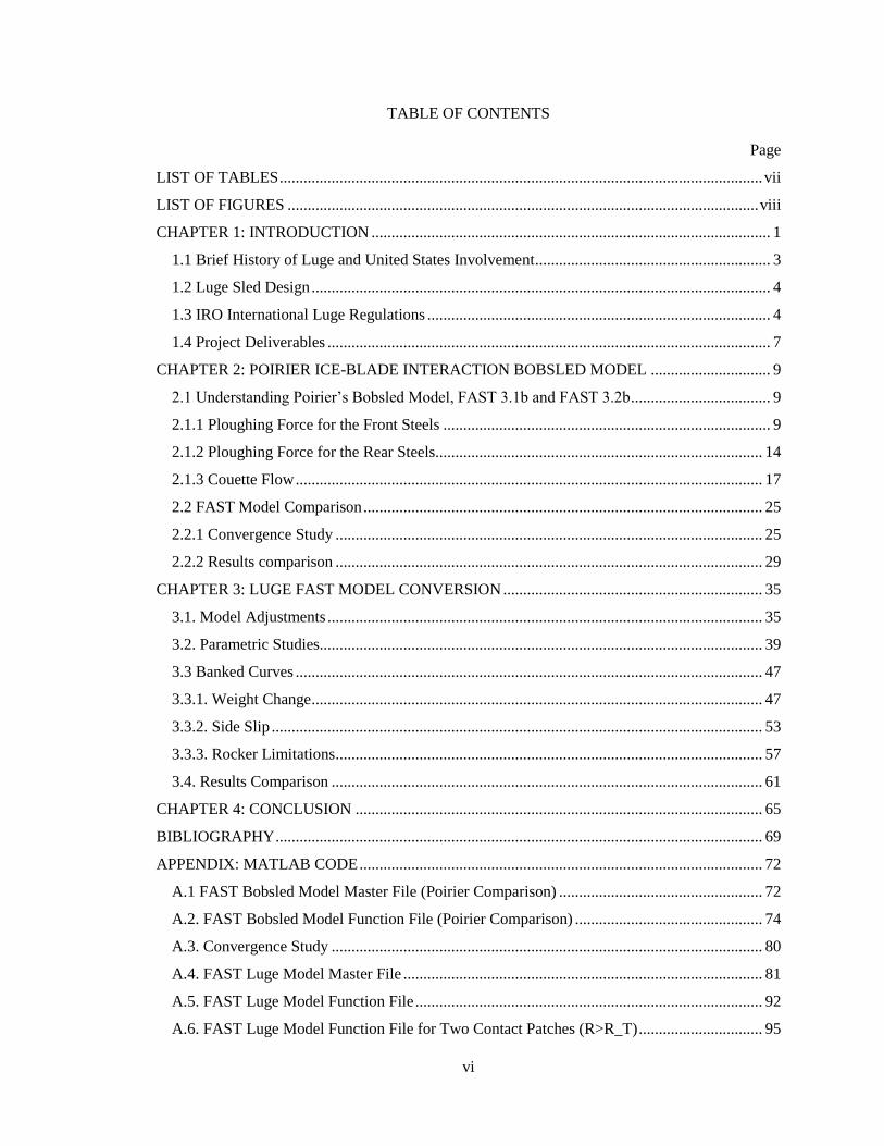
TABLE OF CONTENTS

Page

LIST OF TABLES ......................................................................................................................... vii

LIST OF FIGURES ...................................................................................................................... viii

CHAPTER 1: INTRODUCTION .................................................................................................... 1

1.1 Brief History of Luge and United States Involvement ........................................................... 3

1.2 Luge Sled Design ................................................................................................................... 4

1.3 IRO International Luge Regulations ...................................................................................... 4

1.4 Project Deliverables ............................................................................................................... 7

CHAPTER 2: POIRIER ICE-BLADE INTERACTION BOBSLED MODEL .............................. 9

2.1 Understanding Poirier’s Bobsled Model, FAST 3.1b and FAST 3.2b ................................... 9

2.1.1 Ploughing Force for the Front Steels .................................................................................. 9

2.1.2 Ploughing Force for the Rear Steels.................................................................................. 14

2.1.3 Couette Flow ..................................................................................................................... 17

2.2 FAST Model Comparison .................................................................................................... 25

2.2.1 Convergence Study ........................................................................................................... 25

2.2.2 Results comparison ........................................................................................................... 29

CHAPTER 3: LUGE FAST MODEL CONVERSION ................................................................. 35

3.1. Model Adjustments ............................................................................................................. 35

3.2. Parametric Studies............................................................................................................... 39

3.3 Banked Curves ..................................................................................................................... 47

3.3.1. Weight Change ................................................................................................................. 47

3.3.2. Side Slip ........................................................................................................................... 53

3.3.3. Rocker Limitations ........................................................................................................... 57

3.4. Results Comparison ............................................................................................................ 61

CHAPTER 4: CONCLUSION ...................................................................................................... 65

BIBLIOGRAPHY .......................................................................................................................... 69

APPENDIX: MATLAB CODE ..................................................................................................... 72

A.1 FAST Bobsled Model Master File (Poirier Comparison) ................................................... 72

A.2. FAST Bobsled Model Function File (Poirier Comparison) ............................................... 74

A.3. Convergence Study ............................................................................................................ 80

A.4. FAST Luge Model Master File .......................................................................................... 81

A.5. FAST Luge Model Function File ....................................................................................... 92

A.6. FAST Luge Model Function File for Two Contact Patches (R>R_T) ............................... 95

vii

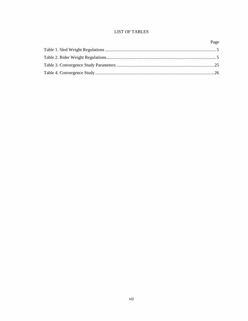
LIST OF TABLES

Page

Table 1. Sled Weight Regulations ................................................................................................... 5

Table 2. Rider Weight Regulations .................................................................................................. 5

Table 3. Convergence Study Parameters ....................................................................................... 25

Table 4. Convergence Study .......................................................................................................... 26

viii

LIST OF FIGURES

Page

Figure 1. USA Luge Run [1] ............................................................................................................ 1

Figure 2. Luge Start: (A)Block (B)Compression (C)Pull (D)Extension (E)Push (F)Paddle [3] ..... 2

Figure 3. Luge Sled Design [5] ........................................................................................................ 4

Figure 4. Steel Dimensions [6] ........................................................................................................ 6

Figure 5. Bobsled Steel .................................................................................................................. 10

Figure 6. Section View A-A' .......................................................................................................... 11

Figure 7. Section View B-B' .......................................................................................................... 12

Figure 8. Front Steel Contact Patch ............................................................................................... 13

Figure 9. Rear Steel Contact Patch ................................................................................................ 14

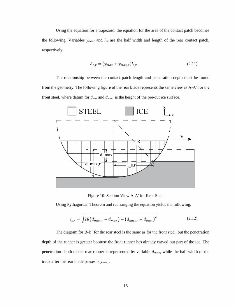
Figure 10. Section View A-A' for Rear Steel ................................................................................ 15

Figure 11. Section View B-B' for Rear Steel ................................................................................. 16

Figure 12. Steel-Ice Couette Flow ................................................................................................. 17

Figure 13. Power Transfer within a Fluid Element ........................................................................ 20

Figure 14. Squeeze Flow................................................................................................................ 23

Figure 15. Convergence Study. ...................................................................................................... 26

Figure 16. Convergence Study Computation Time ....................................................................... 27

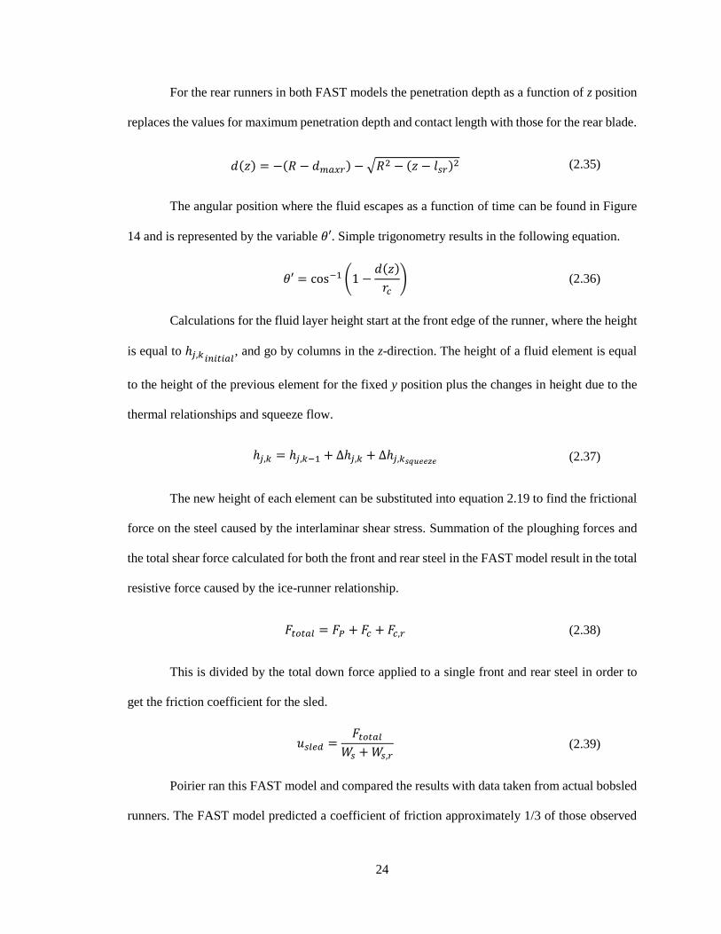
Figure 17. Front Runner Contact Patch Fluid Layer Height .......................................................... 28

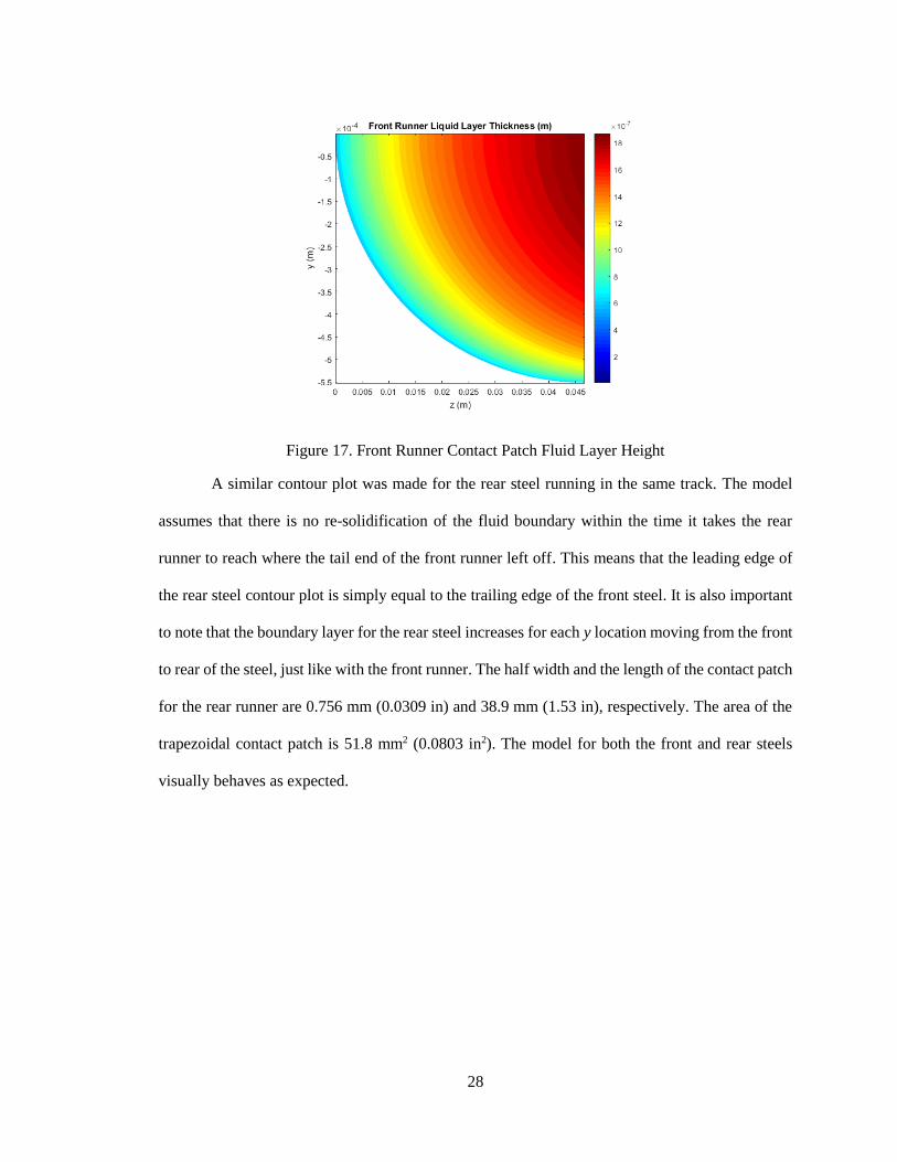
Figure 18. Rear Runner Contact Patch Fluid Layer Height ........................................................... 29

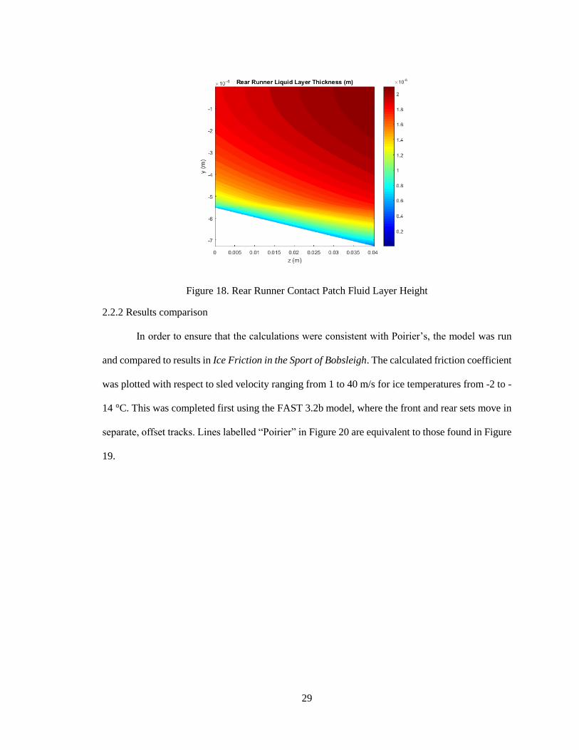
Figure 19. Poirier Figure 4.11 [9] .................................................................................................. 30

Figure 20. Poirier (C++) and Stell (Matlab) FAST 3.2b Model Comparison ................................ 32

Figure 21. Percent Difference Calculations for FAST 3.2b ........................................................... 33

Figure 22. Poirier Figure 4.10 [9] .................................................................................................. 33

Figure 23. Poirier (C++) and Stell (Matlab) FAST Model Comparison for FAST 3.1b ............... 34

Figure 24. Percent Difference Calculations for FAST 3.1b ........................................................... 34

Figure 25. Coefficient of Friction versus Sled Speed for Various Ice Temperatures .................... 36

Figure 26. Coefficient of Friction Percent Difference for Various Ice Temperatures ................... 37

Figure 27. Friction Force for Various Ice Temperatures ............................................................... 38

Figure 28. Percentage of Friction for Various Ice Temperatures ................................................... 39

Figure 29. Coefficient of Friction versus Sled Speed for Various Steel Edge Radii ..................... 40

Figure 30. Coefficient of Friction Percent Difference for Various Steel Edge Radii .................... 41

Figure 31. Friction Force for Various Steel Edge Radii ................................................................ 42

Figure 32. Percentage of Friction for Various Steel Edge Radii.................................................... 43

ix

Figure 33. Coefficient of Friction versus Sled Speed for Various Rockers ................................... 44

Figure 34. Coefficient of Friction Percent Difference for Various Rockers .................................. 44

Figure 35. Friction Force for Various Rockers .............................................................................. 46

Figure 36. Percentage of Friction for Various Rockers ................................................................. 47

Figure 37. Coefficient of Friction versus Sled Speed for Various Sled Weights........................... 48

Figure 38. Coefficient of Friction Percent Difference for Various Sled Weights.......................... 49

Figure 39. Friction Force for Various Sled Weights ...................................................................... 50

Figure 40. Total Friction Force for Various Sled Weights ............................................................ 51

Figure 41. Friction Force Ratios .................................................................................................... 52

Figure 42. Percentage of Friction for Various Sled Weights ......................................................... 53

Figure 43. Side Slip Force Cross Sectional Area ........................................................................... 54

Figure 44. Lateral Force Shear Limit as a Function of Ice Temperature and Rocker .................... 55

Figure 45. Lateral Force Limit as a Function of Ice Temperature and Edge Radius ..................... 56

Figure 46. Lateral Force Limit as a Function of Ice Temperature and Down Force ..................... 56

Figure 47. Track Curve .................................................................................................................. 57

Figure 48. Coefficient of Friction versus Sled Speed Contact Patch Effect .................................. 58

Figure 49. Friction Force Contact Patch Effect ............................................................................. 59

Figure 50. Percentage of Friction Contact Patch Effect ................................................................. 60

Figure 51. Lateral Force Limit versus Ice Temperature Contact Patch Effect .............................. 61

Figure 52. Fauve, Rhyner Figure 4 [11]......................................................................................... 62

Figure 53. Effect of Penetration Depth on Coefficient of Friction ................................................ 62

Figure 54. Effect of Penetration Depth on Coefficient of Friction Zoomed .................................. 64

1

CHAPTER 1: INTRODUCTION

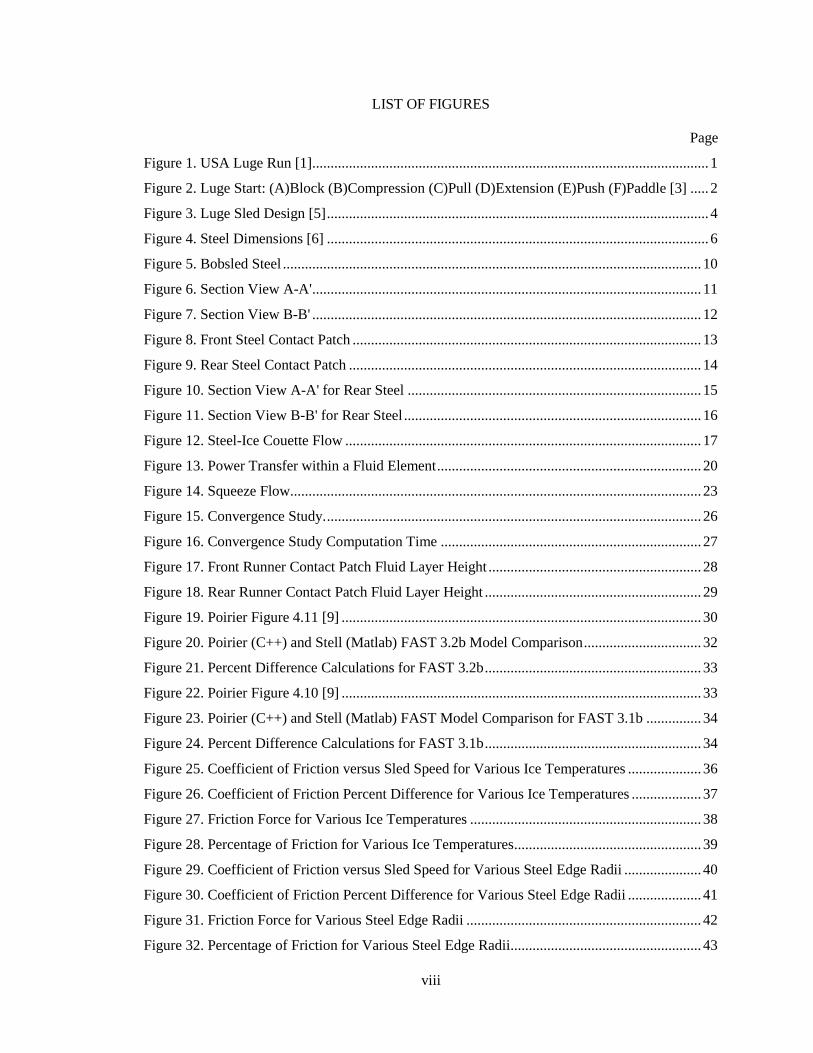
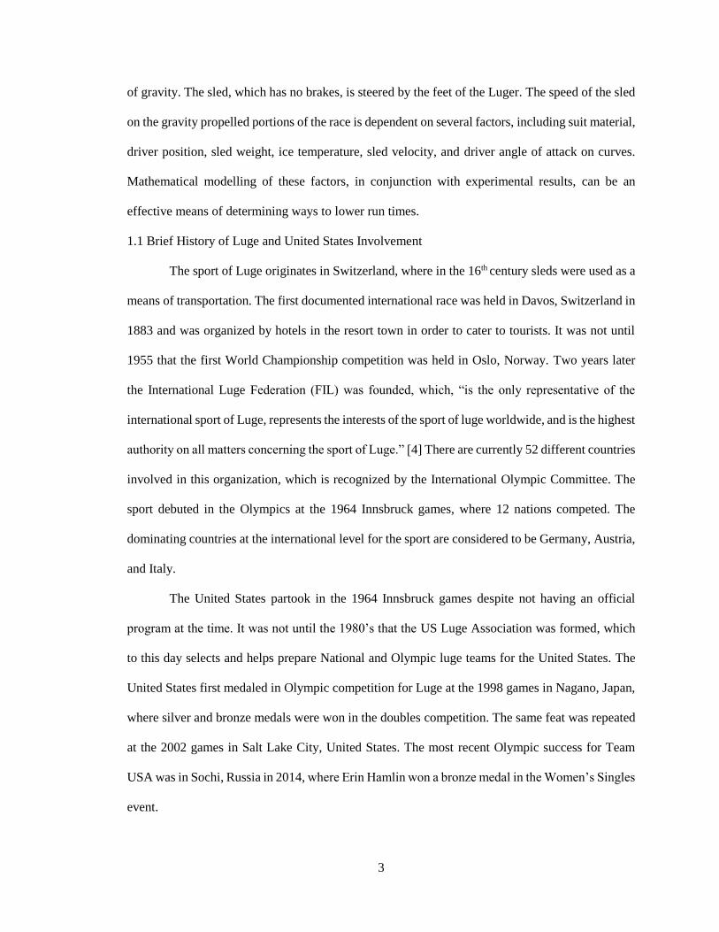
Luge is a sport in which competitors use a sled to slide feet first down an ice chute. Athletes

compete in doubles, singles, and team relay events in order to get the fastest times, which are

measured in thousandths of a second. Sleds can reach speeds of 90 mph.

Figure 1. USA Luge Run [1]

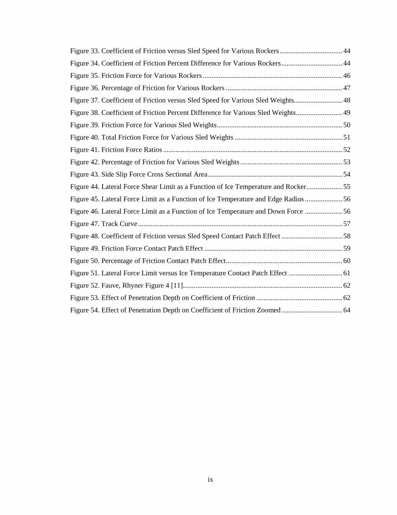
A run in Luge can be broken into two phases, which are the start and the main run. The

start, which is the most crucial portion of a run, has six steps: block, compression, pull, extension,

push, and paddle (see Figure 2). The block is when the athlete, holding onto the start handles, rocks

forward in order to prepare for the starting motion. Compression begins when the competitor slides

the sled backwards with their hips as their knees spread apart and ends when their upper body is

fully compressed between the knees. Pull occurs when the body bounces back from the

compression position, beginning to raise the upper body out from between the legs. During the

extension phase, the athlete uses their back and hip muscles in order to continue moving the sled

forward. Once the hips are in line with the start handles, the push phase begins where the upper

body is kept at an angle of 90 degrees relative to the sled while pushing off from the start handles.

The last stage is the paddle, which is where spiked gloves are used to accelerate the sled down the

starting ramp. The effectiveness of a start is dependent on a combination of technique and physical

2

strength, and must be repeatedly practiced to become a competitive Luger. In the realm of

competitive Luge racing, “it is widely believed that a .01 second advantage at the start can multiply

to a .03 second advantage at the finish,” [2] which is significant in a sport that often has thousandths

of a second differences between race times.

(A)

(B)

(C)

(D)

(E)

(F)

Figure 2. Luge Start: (A)Block (B)Compression (C)Pull (D)Extension (E)Push (F)Paddle [3]

After the athlete gets their sled up to speed, they go into the race position and enter the

banked turns of the course. After this point, the only energy added to the sled is through the force

3

of gravity. The sled, which has no brakes, is steered by the feet of the Luger. The speed of the sled

on the gravity propelled portions of the race is dependent on several factors, including suit material,

driver position, sled weight, ice temperature, sled velocity, and driver angle of attack on curves.

Mathematical modelling of these factors, in conjunction with experimental results, can be an

effective means of determining ways to lower run times.

1.1 Brief History of Luge and United States Involvement

The sport of Luge originates in Switzerland, where in the 16th century sleds were used as a

means of transportation. The first documented international race was held in Davos, Switzerland in

1883 and was organized by hotels in the resort town in order to cater to tourists. It was not until

1955 that the first World Championship competition was held in Oslo, Norway. Two years later

the International Luge Federation (FIL) was founded, which, “is the only representative of the

international sport of Luge, represents the interests of the sport of luge worldwide, and is the highest

authority on all matters concerning the sport of Luge.” [4] There are currently 52 different countries

involved in this organization, which is recognized by the International Olympic Committee. The

sport debuted in the Olympics at the 1964 Innsbruck games, where 12 nations competed. The

dominating countries at the international level for the sport are considered to be Germany, Austria,

and Italy.

The United States partook in the 1964 Innsbruck games despite not having an official

program at the time. It was not until the 1980’s that the US Luge Association was formed, which

to this day selects and helps prepare National and Olympic luge teams for the United States. The

United States first medaled in Olympic competition for Luge at the 1998 games in Nagano, Japan,

where silver and bronze medals were won in the doubles competition. The same feat was repeated

at the 2002 games in Salt Lake City, United States. The most recent Olympic success for Team

USA was in Sochi, Russia in 2014, where Erin Hamlin won a bronze medal in the Women’s Singles

event.

4

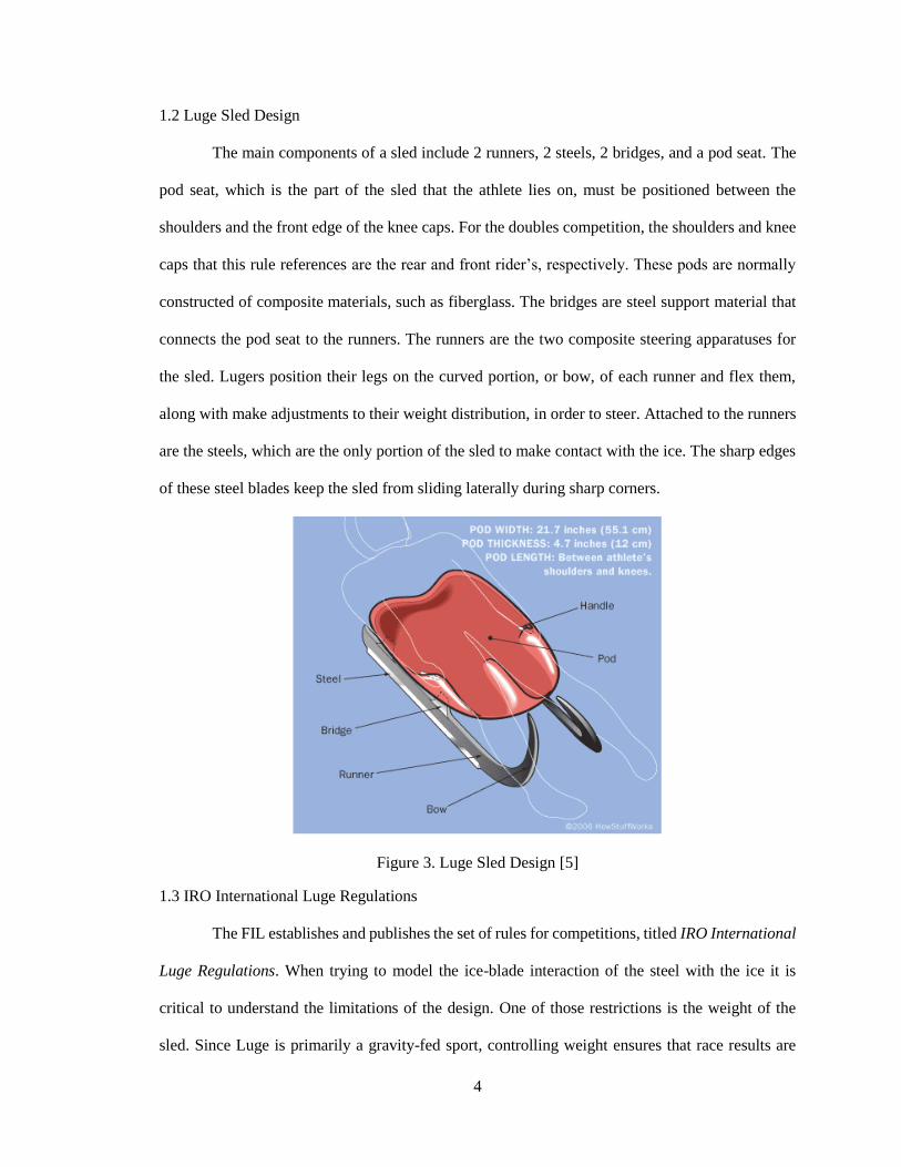
1.2 Luge Sled Design

The main components of a sled include 2 runners, 2 steels, 2 bridges, and a pod seat. The

pod seat, which is the part of the sled that the athlete lies on, must be positioned between the

shoulders and the front edge of the knee caps. For the doubles competition, the shoulders and knee

caps that this rule references are the rear and front rider’s, respectively. These pods are normally

constructed of composite materials, such as fiberglass. The bridges are steel support material that

connects the pod seat to the runners. The runners are the two composite steering apparatuses for

the sled. Lugers position their legs on the curved portion, or bow, of each runner and flex them,

along with make adjustments to their weight distribution, in order to steer. Attached to the runners

are the steels, which are the only portion of the sled to make contact with the ice. The sharp edges

of these steel blades keep the sled from sliding laterally during sharp corners.

Figure 3. Luge Sled Design [5]

1.3 IRO International Luge Regulations

The FIL establishes and publishes the set of rules for competitions, titled IRO International

Luge Regulations. When trying to model the ice-blade interaction of the steel with the ice it is

critical to understand the limitations of the design. One of those restrictions is the weight of the

sled. Since Luge is primarily a gravity-fed sport, controlling weight ensures that race results are

5

determined by driver skill, rather than by who is the heaviest contestant. Table 1 shows the

minimum and maximum allowable sled weights for singles and doubles events including all

attached accessories, as well as the basis for sled weight calculations. If the weight of the sled is

greater than the basis, the difference between the sled weight and the basis must be subtracted from

the allowable additional weight attached to the rider.

Table 1. Sled Weight Regulations

Event Minimum Maximum Basis

Singles 21 kg 25 kg 23 kg

Doubles 25 kg 30 kg 27 kg

The additional weight attached to the rider is dependent on the difference in weight between

the established base weight for that competition and the athlete. For the event, the allowable

additional weight is equal to the percentage of the difference between the base weight and the

Luger’s body weight, up to the maximum additional weight. In the case of doubles competition, if

the weight of both riders is greater than 180 kg, no additional weight may be added. Weigh-ins of

athletes are completed approximately 2 to 3 times in a season.

Table 2. Rider Weight Regulations

Event Base Weight Percentage Maximum

Additional Weight

Women Singles 75 kg 100% 10 kg

Men Singles 90 kg 100% 13 kg

Doubles 90 kg 75% 10 kg

The dimensions of the runner and steel assembly are controlled as well. In the interest of

safety, the edge of the steel must be rounded to a radius of at least 5 mm. Adjustments can be made

to the angle that the blade mounts relative to the runner mounting surface by including a continuous

inlay that can have a maximum thickness of 1 mm and width of 10 mm.

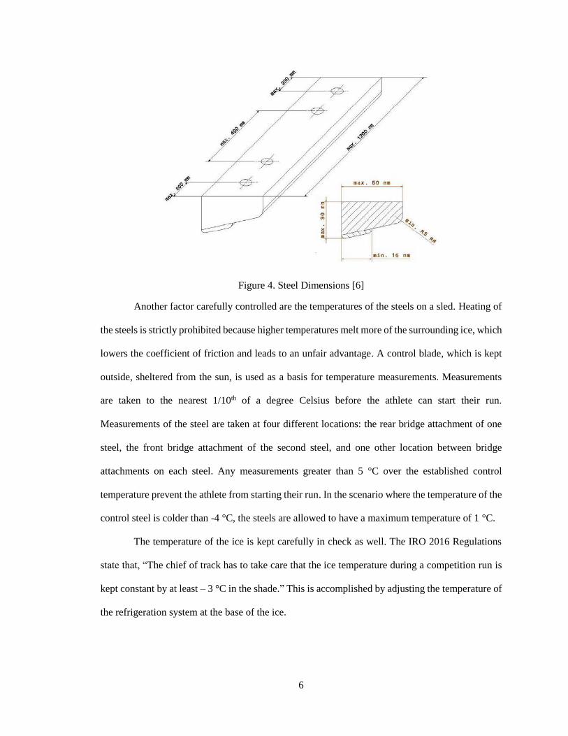
6

Figure 4. Steel Dimensions [6]

Another factor carefully controlled are the temperatures of the steels on a sled. Heating of

the steels is strictly prohibited because higher temperatures melt more of the surrounding ice, which

lowers the coefficient of friction and leads to an unfair advantage. A control blade, which is kept

outside, sheltered from the sun, is used as a basis for temperature measurements. Measurements

are taken to the nearest 1/10th of a degree Celsius before the athlete can start their run.

Measurements of the steel are taken at four different locations: the rear bridge attachment of one

steel, the front bridge attachment of the second steel, and one other location between bridge

attachments on each steel. Any measurements greater than 5 °C over the established control

temperature prevent the athlete from starting their run. In the scenario where the temperature of the

control steel is colder than -4 °C, the steels are allowed to have a maximum temperature of 1 °C.

The temperature of the ice is kept carefully in check as well. The IRO 2016 Regulations

state that, “The chief of track has to take care that the ice temperature during a competition run is

kept constant by at least – 3 °C in the shade.” This is accomplished by adjusting the temperature of

the refrigeration system at the base of the ice.

7

1.4 Project Deliverables

Success in the sport of Luge is a combination between driver skill and optimization of sled

parameters. Adjustments to sleds conventionally have been made after a series of runs where

athletes provide feedback. Inconsistencies in data are often caused by uncontrollable factors such

as driver error, changing temperatures, and varying ice conditions. Development of a driver model

and track model may prove to be useful in order to find more accurate links between sled parameters

and performance in competition. These models are to be developed based off of code made by

Braghin et al. [7] and Mössner et al. [8]. As a part of the driver model in [7], the interaction between

the ice and the runners on the sled will need to be defined. Going into further depth on ice-steel

friction properties will be the primary focus of this project. The basis of this project will be work

completed by Louis Poirier in his thesis, Ice Friction in the Sport of Bobsleigh [9]. Poirier

developed a model for bobsled to capture the frictional properties of the ice-blade interaction as a

sled goes down a straight, constant decline section of track, labelled FAST 3.1b and 3.2b. FAST is

an acronym, which stands for Frictional Algorithm using Skate Thermodynamics. The first step

will be to recreate this model in numerical simulation and compare the results to Poirier’s. Once

this is complete, the numerical model can be adapted to apply to the sport of Luge. This will include

adjusting the geometry of the steels to follow the rules established in the IRO International Luge

Regulations. Within the allowable geometric bounds, a parametric study will be completed in order

to determine qualitatively how blade geometry affects the coefficient of friction. The model will

also add the effect of banked turns on the frictional properties of the sled. This includes the change

in the size of the contact patch from the adjustment in the weight distribution and total down force

on the blades. Sharp turns also raise the concern of lateral deformation of the ice surface, leading

to increases in run times. Identifying the maximum lateral forces the sled can experience without

laterally slipping will be a vital part of the model during turns as well. Calculation of the frictional

properties and lateral force limitations for Luge steels under a variety of conditions, including

changes in downforce, ice temperature, sled velocity, and steel geometry may eventually be used

8

within the Luge dynamic model, being developed separately from this work. Outputs from the

dynamic model may be used, along with experimental data, in order to determine optimum blade

geometries for various race conditions.

9

CHAPTER 2: POIRIER ICE-BLADE INTERACTION BOBSLED MODEL

2.1 Understanding Poirier’s Bobsled Model, FAST 3.1b and FAST 3.2b

Low friction between ice and other materials around its melting point is caused by a thin

film of water that forms between the slider and the ice surface. The formation of this water layer is

primarily a result of frictional heating. The interaction between ice and a skate blade for speed

skating was developed by Penny et al. [10] and was called the FAST 1.0 model, which stands for

Frictional Algorithm using Skate Thermodynamics. Louis Poirier [9] adjusted this model in order

to apply to the sport of Bobsleigh. His goal was to simulate the friction of a bobsled on a straight

section of track with a constant decline. Poirier developed two models: FAST 3.1b and FAST 3.2b.

FAST 3.1b assumed that front and rear runners follow the same tracks, while FAST 3.2b assumed

that the front and rear runners run in parallel tracks. In the case of FAST 3.1b, the assumption was

made that solidification of the melt layer was negligible during the time it takes the rear runner to

span the gap between the front and rear runners. The two major components contributing to the

friction force in the model are the ploughing force of the runners and the Couette flow between the

runners and the ice surface. The ploughing force is the force on the runners from cutting through

the ice surface, while Couette flow is the laminar flow of a viscous liquid between a moving and

stationary surface. The velocity gradient in the fluid boundary layer, which is a characteristic of

Couette flow, results in interlaminar shearing and adds to the total resistive force on the steel.

2.1.1 Ploughing Force for the Front Steels

The ploughing force is the force exerted on the runners as the front section cuts through

the ice. This is a function of the cross sectional area perpendicular to the sled’s motion that the

runner cuts through the ice and the hardness of the ice.

𝐹𝑃 = 𝑃𝐼𝐴𝑃 (2.1)

Poirier determined the hardness of ice through tests run at the Calgary Olympic Oval long

track rink. Steel balls of various sizes were dropped from multiple heights onto the ice surface.

Measurements of the resulting craters, along with measurements of the indentation of an actual

10

bobsled going down the track, at different temperatures resulted in a linear relationship between

temperature, 𝑇, in degrees Celsius and ice hardness, 𝑃𝐼, in megapascal, found in Equation 2.2.

Poirier stated that this fit to the data will not apply to temperatures hotter than -1 degree Celsius

because of the rapid decrease in hardness as the melting point gets closer.

𝑃𝐼 = ((−0.6 ± 0.4)𝑇 + (14.7 ± 2.1))𝑀𝑃𝑎 (2.2)

The perpendicular cross sectional area through which the steels plow through the ice is

dependent on the geometry of the steels and the weight of the sled. The geometry of the bobsled

steels, for simplification, were assumed to have a set rocker and edge radii. Rocker is the radius of

the curvature of the blade along the length of the blade. The rocker and edge radius in Poirier’s

analysis was set to 34 m and 5.5 mm, respectively. In addition, the bobsled was defined as having

a total weight of 390 kg, with 44% applying to the front steels and 56% to the rear steels.

In order to determine the formula of the cross sectional area that the runner cuts through

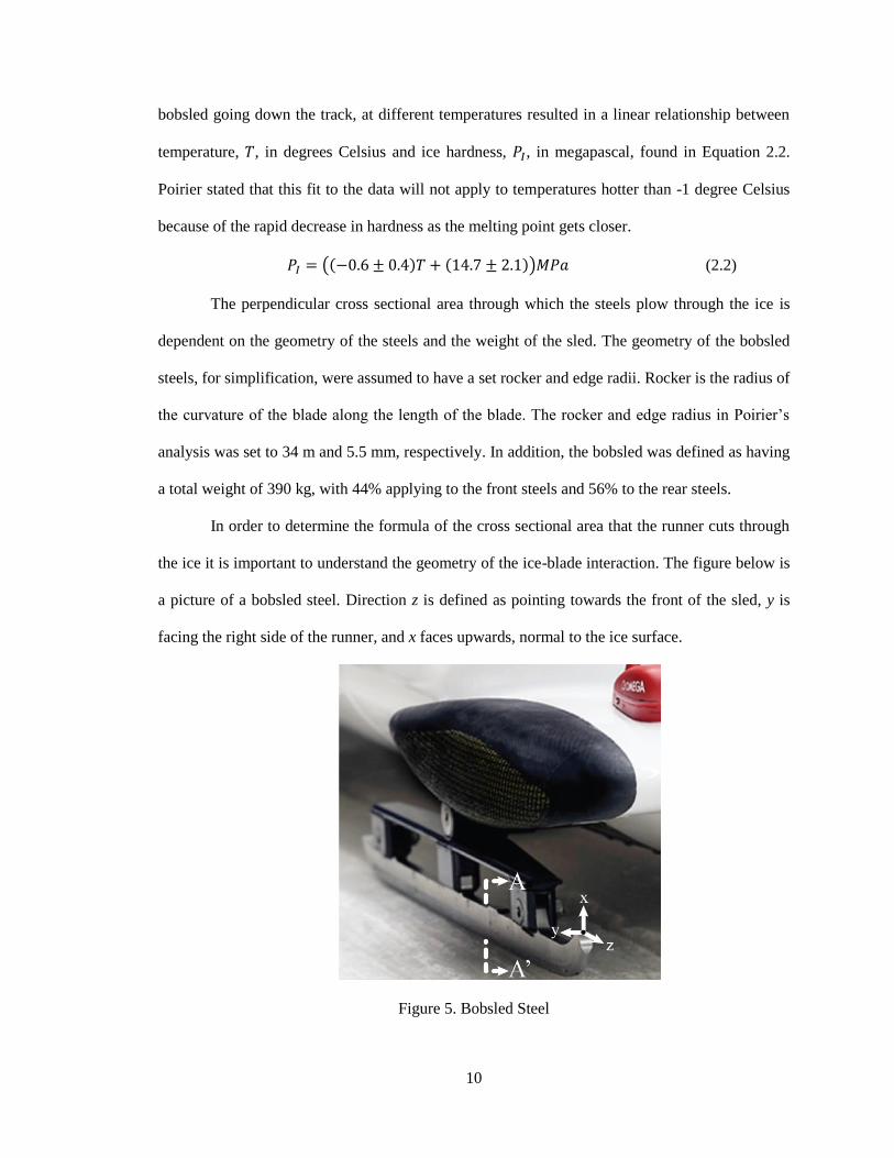
the ice it is important to understand the geometry of the ice-blade interaction. The figure below is

a picture of a bobsled steel. Direction z is defined as pointing towards the front of the sled, y is

facing the right side of the runner, and x faces upwards, normal to the ice surface.

Figure 5. Bobsled Steel

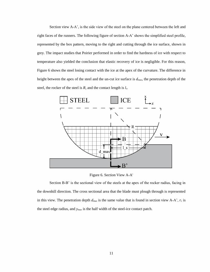
11

Section view A-A’, is the side view of the steel on the plane centered between the left and

right faces of the runners. The following figure of section A-A’ shows the simplified steel profile,

represented by the box pattern, moving to the right and cutting through the ice surface, shown in

grey. The impact studies that Poirier performed in order to find the hardness of ice with respect to

temperature also yielded the conclusion that elastic recovery of ice is negligible. For this reason,

Figure 6 shows the steel losing contact with the ice at the apex of the curvature. The difference in

height between the apex of the steel and the un-cut ice surface is dmax, the penetration depth of the

steel, the rocker of the steel is R, and the contact length is ls.

Figure 6. Section View A-A'

Section B-B’ is the sectional view of the steels at the apex of the rocker radius, facing in

the downhill direction. The cross sectional area that the blade must plough through is represented

in this view. The penetration depth dmax is the same value that is found in section view A-A’, rc is

the steel edge radius, and ymax is the half width of the steel-ice contact patch.

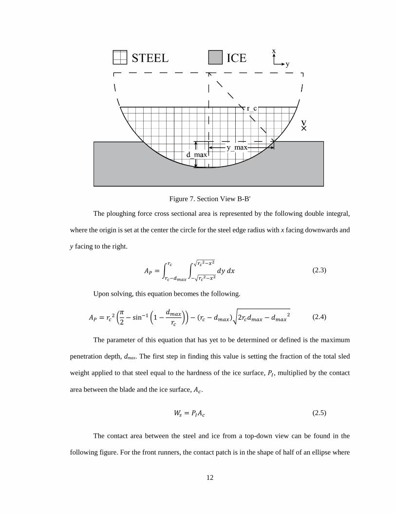
12

Figure 7. Section View B-B'

The ploughing force cross sectional area is represented by the following double integral,

where the origin is set at the center the circle for the steel edge radius with x facing downwards and

y facing to the right.

𝐴𝑃 = ∫ ∫ 𝑑𝑦 𝑑𝑥√𝑟𝑐

2−𝑥2

−√𝑟𝑐2−𝑥2

𝑟𝑐

𝑟𝑐−𝑑𝑚𝑎𝑥

(2.3)

Upon solving, this equation becomes the following.

𝐴𝑃 = 𝑟𝑐2 (

𝜋

2− sin−1 (1 −

𝑑𝑚𝑎𝑥

𝑟𝑐)) − (𝑟𝑐 − 𝑑𝑚𝑎𝑥)√2𝑟𝑐𝑑𝑚𝑎𝑥 − 𝑑𝑚𝑎𝑥

2 (2.4)

The parameter of this equation that has yet to be determined or defined is the maximum

penetration depth, dmax. The first step in finding this value is setting the fraction of the total sled

weight applied to that steel equal to the hardness of the ice surface, 𝑃𝐼, multiplied by the contact

area between the blade and the ice surface, 𝐴𝑐.

𝑊𝑠 = 𝑃𝐼𝐴𝑐 (2.5)

The contact area between the steel and ice from a top-down view can be found in the

following figure. For the front runners, the contact patch is in the shape of half of an ellipse where

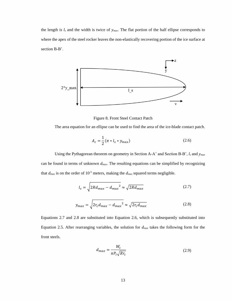
13

the length is ls and the width is twice of ymax. The flat portion of the half ellipse corresponds to

where the apex of the steel rocker leaves the non-elastically recovering portion of the ice surface at

section B-B’.

Figure 8. Front Steel Contact Patch

The area equation for an ellipse can be used to find the area of the ice-blade contact patch.

𝐴𝑐 =1

2(𝜋 ∗ 𝑙𝑠 ∗ 𝑦𝑚𝑎𝑥) (2.6)

Using the Pythagorean theorem on geometry in Section A-A’ and Section B-B’, ls and ymax

can be found in terms of unknown dmax. The resulting equations can be simplified by recognizing

that dmax is on the order of 10-5 meters, making the dmax squared terms negligible.

𝑙𝑠 = √2𝑅𝑑𝑚𝑎𝑥 − 𝑑𝑚𝑎𝑥2 ≈ √2𝑅𝑑𝑚𝑎𝑥 (2.7)

𝑦𝑚𝑎𝑥 = √2𝑟𝑐𝑑𝑚𝑎𝑥 − 𝑑𝑚𝑎𝑥2 ≈ √2𝑟𝑐𝑑𝑚𝑎𝑥 (2.8)

Equations 2.7 and 2.8 are substituted into Equation 2.6, which is subsequently substituted into

Equation 2.5. After rearranging variables, the solution for dmax takes the following form for the

front steels.

𝑑𝑚𝑎𝑥 =𝑊𝑠

𝜋𝑃𝐼√𝑅𝑟𝑐

(2.9)

14

Equation 2.9 can be substituted into Equation 2.4 to solve for the cross sectional area the

front runner must cut through. This, along with the solution from Equation 2.2, can be placed into

Equation 2.1 to find the ploughing force of just the front runner.

2.1.2 Ploughing Force for the Rear Steels

For the model FAST 3.2b, where the front and rear runners follow separate tracks, the

weight distributed on the rear steels, along with the same sets of equations, can be used to find the

rear penetration depth. This value can be substituted into Equation 2.4, which can, along with

Equation 2.2, be substituted into Equation 2.1 to find the ploughing force of just the rear runner.

In the case where the front and rear runners run in the same tracks, as seen in FAST 3.1b,

the penetration depth of the rear steel is affected by penetration depth of the front steel. The rear

steel continues cutting deeper into the ice surface, meaning that the cross sectional area that the rear

steel leaves carved from the ice surface, AP,r, encompasses the area cut by the front steel plus the

additional depth cut by the rear steel. This means that in the case of FAST 3.1b the total ploughing

force equation, including both front and rear blades, takes the following form.

𝐹𝑃 = 𝑃𝐼𝐴𝑃,𝑟 (2.10)

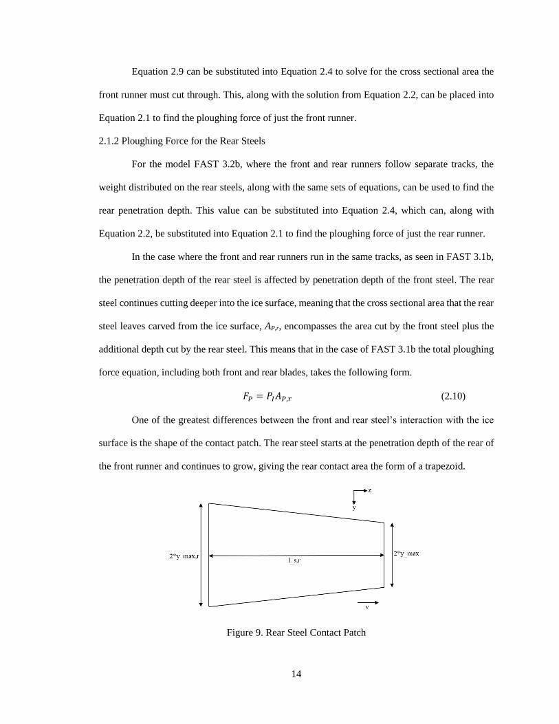
One of the greatest differences between the front and rear steel’s interaction with the ice

surface is the shape of the contact patch. The rear steel starts at the penetration depth of the rear of

the front runner and continues to grow, giving the rear contact area the form of a trapezoid.

Figure 9. Rear Steel Contact Patch

15

Using the equation for a trapezoid, the equation for the area of the contact patch becomes

the following. Variables ymax,r and ls,r are the half width and length of the rear contact patch,

respectively.

𝐴𝑐,𝑟 = (𝑦𝑚𝑎𝑥 + 𝑦𝑚𝑎𝑥,𝑟)𝑙𝑠,𝑟 (2.11)

The relationship between the contact patch length and penetration depth must be found

from the geometry. The following figure of the rear blade represents the same view as A-A’ for the

front steel, where datum for dmax and dmax,r is the height of the pre-cut ice surface.

Figure 10. Section View A-A' for Rear Steel

Using Pythagorean Theorem and rearranging the equation yields the following.

𝑙𝑠,𝑟 = √2𝑅(𝑑𝑚𝑎𝑥,𝑟 − 𝑑𝑚𝑎𝑥) − (𝑑𝑚𝑎𝑥,𝑟 − 𝑑𝑚𝑎𝑥)2 (2.12)

The diagram for B-B’ for the rear steel is the same as for the front steel, but the penetration

depth of the runner is greater because the front runner has already carved out part of the ice. The

penetration depth of the rear runner is represented by variable dmax,r, while the half width of the

track after the rear blade passes is ymax,r.

16

Figure 11. Section View B-B' for Rear Steel

The geometry in section view B-B’ for the rear steel is the exact same setup as that seen

for the front steel, leading the form of the equation for ymax,r to be the exact same as ymax, but with

dmax,r substituted for dmax.

𝑦𝑚𝑎𝑥,𝑟 = √2𝑟𝑐𝑑𝑚𝑎𝑥,𝑟 − 𝑑𝑚𝑎𝑥,𝑟2 (2.13)

Equation 2.13 and Equation 2.12 can be substituted into Equation 2.11 to find the contact

area of the rear runner.

𝐴𝑐,𝑟 = (𝑦𝑚𝑎𝑥 + √2𝑟𝑐𝑑𝑚𝑎𝑥,𝑟 − 𝑑𝑚𝑎𝑥,𝑟2) √2𝑅(𝑑𝑚𝑎𝑥,𝑟 − 𝑑𝑚𝑎𝑥) − (𝑑𝑚𝑎𝑥,𝑟 − 𝑑𝑚𝑎𝑥)

2 (2.14)

This can be substituted into an equation similar in form to Equation 2.5 to get the following,

which must be solved in terms of dmax,r.

𝑊𝑠,𝑟

𝑃𝐼= (𝑦𝑚𝑎𝑥 + √2𝑟𝑐𝑑𝑚𝑎𝑥,𝑟 − 𝑑𝑚𝑎𝑥,𝑟

2) √2𝑅(𝑑𝑚𝑎𝑥,𝑟 − 𝑑𝑚𝑎𝑥) − (𝑑𝑚𝑎𝑥,𝑟 − 𝑑𝑚𝑎𝑥)2 (2.15)

In order to accomplish this, an iterative solution is necessary, which includes an initial

guess for dmax,r of twice of dmax. The value for the penetration depth of the rear runner is varied until

the left and right sides of Equation 2.15 are within 0.1% of each other. Once the solution for dmax,r

17

is found, it can be used to find the plough area of the rear runner. The form of the rear plough area

equation is found using the same double integral method as the front runner in Equation 2.3.

Equation 2.16 is the same equation as Equation 2.3, but with dmax,r replacing dmax.

𝐴𝑃,𝑟 = 𝑟𝑐2 (

𝜋

2− sin−1 (1 −

𝑑𝑚𝑎𝑥,𝑟

𝑟𝑐)) − (𝑟𝑐 − 𝑑𝑚𝑎𝑥,𝑟)√2𝑟𝑐𝑑𝑚𝑎𝑥,𝑟 − 𝑑𝑚𝑎𝑥,𝑟

2 (2.16)

This solution, along with the value of the ice hardness from Equation 2.2, can then be

substituted into Equation 2.10 to find the total ploughing force on the sled exerted on a single front

and rear steel for the FAST 3.1b model where both front and rear runners follow the same path.

2.1.3 Couette Flow

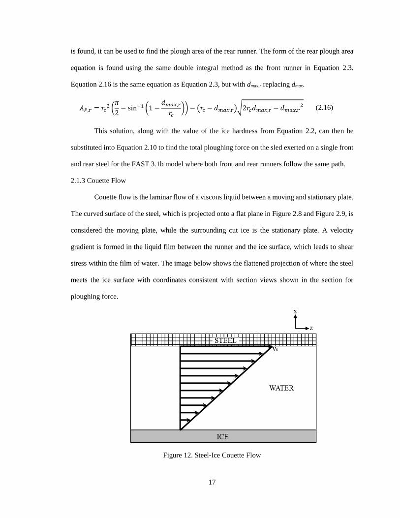
Couette flow is the laminar flow of a viscous liquid between a moving and stationary plate.

The curved surface of the steel, which is projected onto a flat plane in Figure 2.8 and Figure 2.9, is

considered the moving plate, while the surrounding cut ice is the stationary plate. A velocity

gradient is formed in the liquid film between the runner and the ice surface, which leads to shear

stress within the film of water. The image below shows the flattened projection of where the steel

meets the ice surface with coordinates consistent with section views shown in the section for

ploughing force.

Figure 12. Steel-Ice Couette Flow

18

Friction as a result of the interlaminar shear stress can be found from the following equation

for shear strain in a Newtonian fluid, which is dependent on the dynamic viscosity of water and the

slope of the velocity gradient with respect to x. The shear stress equals friction force on the plate

from the Couette flow divided by the area of the contact patch.

𝜏 = 𝜇𝑤

𝑑𝑣

𝑑𝑥=

𝐹𝑐

𝐴𝑐 (2.17)

Rearranging the equation yields the following.

𝐹𝑐 = 𝜇𝑤𝐴𝑐

𝑑𝑣

𝑑𝑥 (2.18)

It is important to note that the interlaminar shear force adds energy to fluid layer, increasing

its size due to the effects of melting. For this reason the height of the fluid layer will be greater at

the rear of the contact patch versus the front. This means that the gradient of the velocity with

respect to x will change depending on the location on the contact patch. In order to take this into

account the contact patch is broken into a mesh and the friction force due to the Couette flow is

calculated for each individual fluid column. Variable ℎ𝑗,𝑘 represents the fluid layer height for a

specific location and ∆𝑦∆𝑧 is the calculation for the area of a single element depending on the

chosen mesh size. The contributing friction force from each fluid column is then summed to get

the total friction force on the steel from the Couette flow.

𝐹𝑐 = ∑ 𝜇𝑤(∆𝑦∆𝑧)𝑣𝑠

ℎ𝑗,𝑘𝑗,𝑘

(2.19)

The remaining variable to calculate is the height for each fluid element. Studies have shown

that a pre-existing, quasi-liquid layer naturally forms on an ice surface. Poirier defined the initial

fluid layer height, which is on the order of nanometers, with Equation 2.20, where 𝑇𝑖 is the ice

surface temperature in degrees Celsius. This layer is present even before the sled contacts the ice,

so the liquid film is equal to the thickness of the pre-existing layer at the front edge of the runner.

19

ℎ𝑗,𝑘𝑖𝑛𝑖𝑡𝑖𝑎𝑙= 3.5(−𝑇𝑖)−1 2.4⁄ 𝑛𝑚 (2.20)

Variations in fluid layer height due to melting are caused by a combination of internal heat

generation from the shear stress between fluid layers and conduction between the water and its

surroundings. The temperature that ice melts at, 𝑇𝑚, is effected by the pressure applied on the

steel, 𝑃𝑠. Increases in pressure applied to the ice corresponds to decreases in the melting point. This

is known as the Clausius-Claperyon relationship. The temperature of the fluid layer for the model,

as well at the neighboring ice, is set at this temperature.

𝑇𝑚 = (−7.37 × 10−8 ℃ 𝑃𝑎⁄ )𝑃𝑠 (2.21)

The energy required in order to completely melt a slab of ice at melting temperature is

dependent on the mass of the ice being melted and the latent heat of fusion of ice.

𝑞 = 𝑚𝑖𝑙𝑓 (2.22)

The mass of the ice that is melted for the element is equal to the density of ice multiplied

by the volume of ice melted. Due to conservation of mass, it is also valid to say that the mass of

the ice melted is equal to the density of water multiplied by the volume of water added to the melt

layer.

𝑞 = (𝜌𝑤∆∀𝑤)𝑙𝑓 (2.23)

The equation for the power required to melt the section of ice and change the fluid layer

height by ∆ℎ𝑗,𝑘 for a single element is the energy, 𝑞, divided by the time period that the energy is

being applied, ∆𝑡. The energy to melt the entire slab of ice for the section must be delivered in the

time that it takes the sled to travel the length of the element, ∆𝑧. This corresponds to the velocity

of the sled, 𝑣𝑠.

20

𝑃 =𝑞

∆𝑡=

𝜌𝑤𝑙𝑓∆𝑧∆𝑦∆ℎ𝑗,𝑘

∆𝑡= 𝜌𝑤𝑙𝑓𝑣𝑠∆𝑦∆ℎ𝑗,𝑘 (2.24)

The power created by the interlaminar shearing of the fluid layer for a single element is

equal to the friction force from the Couette flow within that single element, represented within the

summation for the entire fluid layer in Equation 2.19, multiplied by the velocity of the sled. The

entirety of the power generated is assumed to go into melting the ice slab. Power going into the ice

slab is defined as positive.

𝑃𝑐 = 𝐹𝑐𝑗,𝑘𝑣𝑠 = 𝜇𝑤(∆𝑦∆𝑧)

𝑣𝑠2

ℎ𝑗,𝑘 (2.25)

Three additional factors contributing to the net power transfer into the ice element being

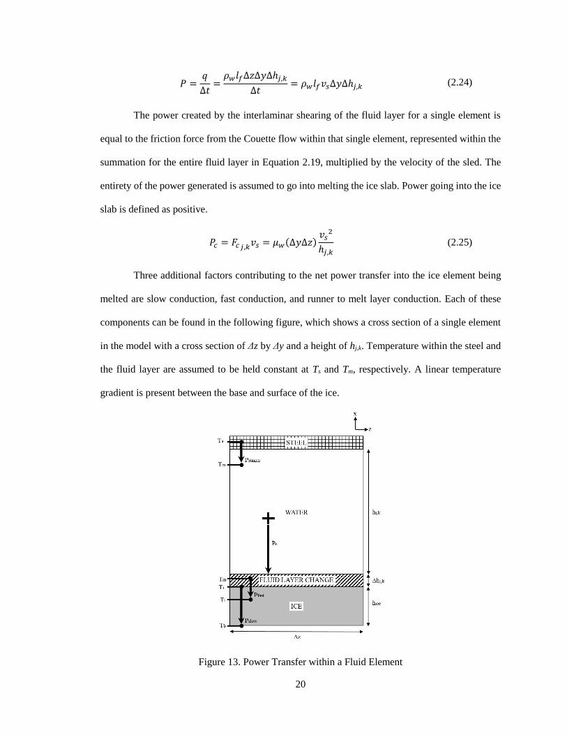
melted are slow conduction, fast conduction, and runner to melt layer conduction. Each of these

components can be found in the following figure, which shows a cross section of a single element

in the model with a cross section of Δz by Δy and a height of hj,k. Temperature within the steel and

the fluid layer are assumed to be held constant at Ts and Tm, respectively. A linear temperature

gradient is present between the base and surface of the ice.

Figure 13. Power Transfer within a Fluid Element

21

Slow conduction is a result of modern day artificial track design and is due to the difference

in temperature between the temperature-controlled base of the ice track and the ice surface. The

thickness of an artificial track ice surface is typically around 25 mm. Poirier, after talks with a

former track manager, decided to set the ice base temperature to be 2 °C lower than the surface

temperature, but has stated that further study to confirm this may be necessary. The equation for

heat flux, defined as the power transferred per unit area, for one-dimensional, steady state heat

conduction with a linear temperature gradient is the following. Variable 𝑘 is the thermal

conductivity, 𝑇1 and 𝑇2 are the temperatures of the boundaries, and 𝐿 is the distance between the

temperature boundaries.

𝑞′′ =𝑃

𝐴= 𝑘

𝑇1 − 𝑇2

𝐿 (2.26)

This can rearranged to calculate the power transferred from boundary 1 to 2.

𝑃 = 𝑘𝑇1 − 𝑇2

𝐿𝐴 (2.27)

For slow conduction the boundary temperatures are the temperature of the ice surface 𝑇𝑖

and the temperature of the ice base 𝑇𝑏, the thermal conductivity is for the ice, the length is the ice

thickness, and the area is the cross sectional area of a single element. Energy is transferred in this

case from the melting ice section to the base, meaning that 𝑃𝑠𝑙𝑜𝑤, using the established convention

of energy into the melting slab is positive, is negative.

𝑃𝑠𝑙𝑜𝑤 = 𝑘𝑖

𝑇𝑏 − 𝑇𝑖

ℎ𝑖𝑐𝑒∆𝑦∆𝑧 (2.28)

Fast conduction is due to the temperature difference between the liquid film and the melting

ice element. This is a transient condition, so it changes as the fluid column moves from the front to

the rear of the contact patch. Power from fast conduction is dependent on the difference in

temperature between the melted ice and the ice surface, velocity of the sled, density of the ice,

22

specific heat of the ice, thermal conductivity of the ice, element cross sectional area, and distance

from the front edge of the steel.

𝑃𝑓𝑎𝑠𝑡 = −𝑘𝑖(𝑇𝑚 − 𝑇𝑖)

√𝜋𝜅𝑖𝑡∆𝑦∆𝑧 = −(𝑇𝑚 − 𝑇𝑖)√

𝑣𝜌𝑖𝑐𝑖𝑘𝑖

𝜋(𝑧𝑜(𝑦) − 𝑧)∆𝑦∆𝑧 (2.29)

Runner to melt layer conduction is due to the temperature difference between the steels

and the liquid layer. The equation for power is similar in form to Equation 2.29, but with the

characteristics of steel replacing ice.

𝑃𝑟𝑢𝑛𝑛𝑒𝑟 =𝑘𝑠(𝑇𝑠 − 𝑇𝑚)

√𝜋𝜅𝑠𝑡∆𝑦∆𝑧 = (𝑇𝑠 − 𝑇𝑚)√

𝑣𝜌𝑠𝑐𝑠𝑘𝑠

𝜋(𝑧𝑜(𝑦) − 𝑧)∆𝑦∆𝑧 (2.30)

Each of these heat transfer and heat generation factors contribute to changes in the size of

the melt layer. Summation of each of these factors equals the total power into the melt layer.

𝑃 = 𝑃𝑐 + 𝑃𝑠𝑙𝑜𝑤 + 𝑃𝑓𝑎𝑠𝑡 + 𝑃𝑟𝑢𝑛𝑛𝑒𝑟 (2.31)

This can be substituted into Equation 2.24, then rearranged to get the change in height of

the fluid element.

∆ℎ𝑗,𝑘 =∆𝑧

𝜌𝑤𝑙𝑓𝑣𝑠(𝜇𝑤

𝑣𝑠2

ℎ𝑗,𝑘−1+ 𝑘𝑖

𝑇𝑏 − 𝑇𝑖

ℎ𝑖𝑐𝑒− (𝑇𝑚 − 𝑇𝑖)√

𝑣𝜌𝑖𝑐𝑖𝑘𝑖

𝜋(𝑧𝑜(𝑦) − 𝑧)+ (𝑇𝑠 − 𝑇𝑚)√

𝑣𝜌𝑠𝑐𝑠𝑘𝑠

𝜋(𝑧𝑜(𝑦) − 𝑧)) (2.32)

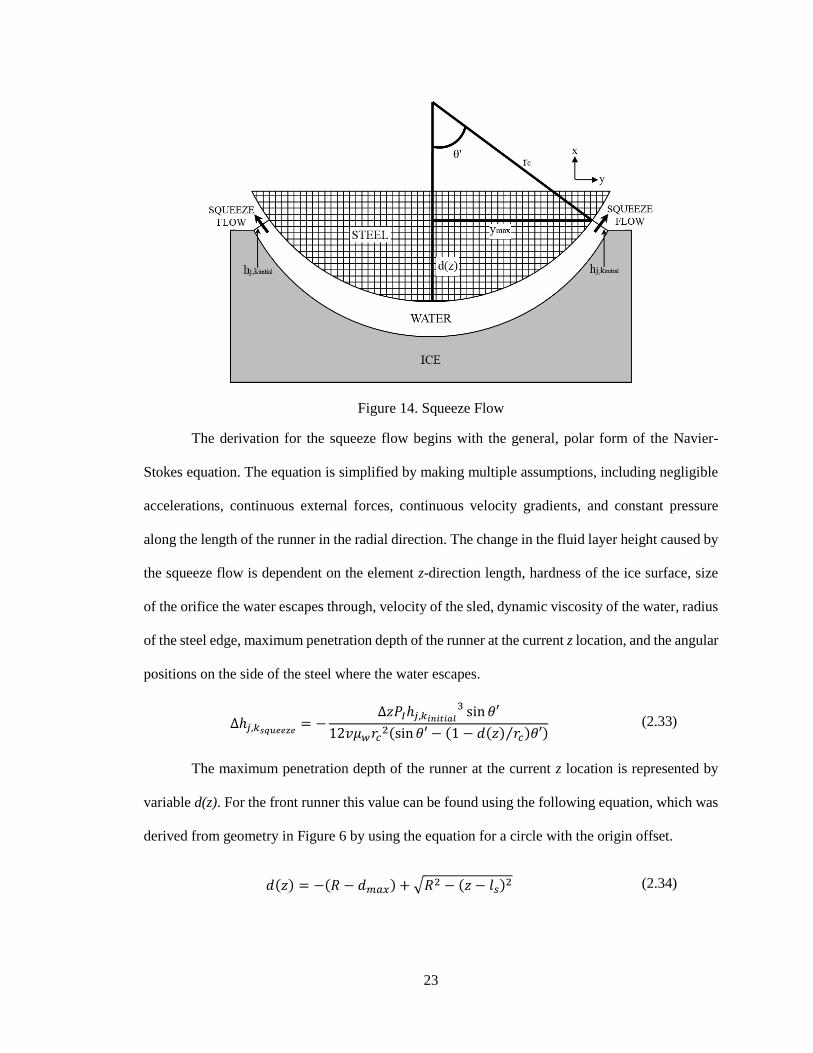
The final factor in this model contributing to melt layer size is the squeeze flow, which

occurs when the runner compresses the liquid layer, pushing some out. The sides of the blade are

considered the significant locations where fluid boundary loss occurs because the contact length of

the steel is so much larger than the contact width. The following figure shows a cross section of the

fluid melt layer between the runner and ice surfaces, as well as the locations where the fluid escapes.

23

Figure 14. Squeeze Flow

The derivation for the squeeze flow begins with the general, polar form of the Navier-

Stokes equation. The equation is simplified by making multiple assumptions, including negligible

accelerations, continuous external forces, continuous velocity gradients, and constant pressure

along the length of the runner in the radial direction. The change in the fluid layer height caused by

the squeeze flow is dependent on the element z-direction length, hardness of the ice surface, size

of the orifice the water escapes through, velocity of the sled, dynamic viscosity of the water, radius

of the steel edge, maximum penetration depth of the runner at the current z location, and the angular

positions on the side of the steel where the water escapes.

∆ℎ𝑗,𝑘𝑠𝑞𝑢𝑒𝑒𝑧𝑒= −

∆𝑧𝑃𝐼ℎ𝑗,𝑘𝑖𝑛𝑖𝑡𝑖𝑎𝑙

3 sin 𝜃′

12𝑣𝜇𝑤𝑟𝑐2(sin 𝜃′ − (1 − 𝑑(𝑧) 𝑟𝑐⁄ )𝜃′)

(2.33)

The maximum penetration depth of the runner at the current z location is represented by

variable d(z). For the front runner this value can be found using the following equation, which was

derived from geometry in Figure 6 by using the equation for a circle with the origin offset.

𝑑(𝑧) = −(𝑅 − 𝑑𝑚𝑎𝑥) + √𝑅2 − (𝑧 − 𝑙𝑠)2 (2.34)

24

For the rear runners in both FAST models the penetration depth as a function of z position

replaces the values for maximum penetration depth and contact length with those for the rear blade.

𝑑(𝑧) = −(𝑅 − 𝑑𝑚𝑎𝑥𝑟) − √𝑅2 − (𝑧 − 𝑙𝑠𝑟)2 (2.35)

The angular position where the fluid escapes as a function of time can be found in Figure

14 and is represented by the variable 𝜃′. Simple trigonometry results in the following equation.

𝜃′ = cos−1 (1 −𝑑(𝑧)

𝑟𝑐) (2.36)

Calculations for the fluid layer height start at the front edge of the runner, where the height

is equal to ℎ𝑗,𝑘𝑖𝑛𝑖𝑡𝑖𝑎𝑙, and go by columns in the z-direction. The height of a fluid element is equal

to the height of the previous element for the fixed y position plus the changes in height due to the

thermal relationships and squeeze flow.

ℎ𝑗,𝑘 = ℎ𝑗,𝑘−1 + ∆ℎ𝑗,𝑘 + ∆ℎ𝑗,𝑘𝑠𝑞𝑢𝑒𝑒𝑧𝑒 (2.37)

The new height of each element can be substituted into equation 2.19 to find the frictional

force on the steel caused by the interlaminar shear stress. Summation of the ploughing forces and

the total shear force calculated for both the front and rear steel in the FAST model result in the total

resistive force caused by the ice-runner relationship.

𝐹𝑡𝑜𝑡𝑎𝑙 = 𝐹𝑃 + 𝐹𝑐 + 𝐹𝑐,𝑟 (2.38)

This is divided by the total down force applied to a single front and rear steel in order to

get the friction coefficient for the sled.

𝑢𝑠𝑙𝑒𝑑 =𝐹𝑡𝑜𝑡𝑎𝑙

𝑊𝑠 + 𝑊𝑠,𝑟 (2.39)

Poirier ran this FAST model and compared the results with data taken from actual bobsled

runners. The FAST model predicted a coefficient of friction approximately 1/3 of those observed

25

in experiments. Possible explanations requiring further research suggested by Poirier included

underestimation of the amount of squeeze flow, runner roughness, and runner vibration.

2.2 FAST Model Comparison

Poirier’s FAST 3.1b and 3.2b models were recreated in Matlab to act as a starting point for

the Luge ice-blade interaction model. This model applies to a bobsled moving on a flat, constant

decline section of track.

2.2.1 Convergence Study

It was recommended by Poirier for numerical convergence that each mesh element have

Δz equal 10-6 meters and Δy equal 10-7 meters. Due to the different coding environment, it was

deemed necessary to perform a convergence study. For this study model parameters were set to the

following.

Table 3. Convergence Study Parameters

Model FAST 3.1b

Sled Velocity 15 m/s

Ice Temperature -10 °C

Rocker 34 m

Edge Radius 5.5 mm

Sled Mass 390 kg

Front/Rear Weight Distribution 44-56

The size of the elements were adjusted in small increments and the resulting coefficient of

friction for the sled was tracked and recorded in Table 4. The total number of elements in both the

front and rear contact patch fluid layer height matrices was increased until the percent difference

between consecutive coefficients of friction was less than 1%. In addition, for each run the amount

of time that it took Matlab to solve was recorded to see how element size effects computation time.

26

Table 4. Convergence Study

Δz

(m)

Δy

(m)

Element

Total

Elapsed Time

(sec)

Coefficient of

Friction, usled (10-3)

Percent Difference

(%)

5*10-4 5*10-5 2340 0.021 0.6160

10-4 10-5 55,856 0.042 0.8201 28.4

5*10-5 5*10-6 222,253 0.088 1.0464 24.2

2*10-5 2*10-6 1,385,764 0.575 1.3429 24.8

1.5*10-5 1.5*10-6 2,463,549 1.034 1.4083 4.75

1.25*10-5 1.25*10-6 3,542,170 1.447 1.4412 2.31

10-5 10-6 5,538,403 2.237 1.4774 2.48

9*10-6 9*10-7 6,833,129 2.806 1.4914 0.94

The model reached convergence when Δz was set to 10-5 meters and Δy to 10-6 meters, a

full order larger than what was recommended for each dimension. The following figure is a plot of

the coefficient of friction with respect to the total number of elements in the solution. The slope of

the plot rapidly decreases and convergence is observed around 5.5 million elements.

Figure 15. Convergence Study.

While the plot of coefficient of friction appears to converge to an asymptote around 0.0015,

the computation time continues to increase. The following figure shows a linear relationship

between calculation time and element total, with a slope of approximately 0.4 microseconds per

element.

27

Figure 16. Convergence Study Computation Time

To ensure that the shape and pattern of the fluid layer is visually consistent with what is

expected a contour plot of the fluid layer thickness was made for the front contact patch. The

following figure shows half of the contact patch displayed in Figure 8 and has the sled moving to

the left, rather than to the right. Colors blue to red correspond to the thinnest to thickest fluid

boundary layer. As expected, the front edge of the contact patch is the thinnest and equals the height

of the pre-existing fluid boundary layer, ℎ𝑗,𝑘𝑖𝑛𝑖𝑡𝑖𝑎𝑙. The height of the boundary layer then continues

to increase for each set y row until reaching a maximum at the rear of the contact patch, where the

blade loses contact with the ice surface. With the current parameters set the half width of the front

contact patch is equal to 0.573 mm (0.0226 in) and the contact length is equal to 45.1 mm (1.78 in).

This corresponds to a contact area of just 40.6 mm2 (0.0629 in2) that the front steel has to grip to

the ice surface, which is equivalent to 14% of the area of a US penny.

28

Figure 17. Front Runner Contact Patch Fluid Layer Height

A similar contour plot was made for the rear steel running in the same track. The model

assumes that there is no re-solidification of the fluid boundary within the time it takes the rear

runner to reach where the tail end of the front runner left off. This means that the leading edge of

the rear steel contour plot is simply equal to the trailing edge of the front steel. It is also important

to note that the boundary layer for the rear steel increases for each y location moving from the front

to rear of the steel, just like with the front runner. The half width and the length of the contact patch

for the rear runner are 0.756 mm (0.0309 in) and 38.9 mm (1.53 in), respectively. The area of the

trapezoidal contact patch is 51.8 mm2 (0.0803 in2). The model for both the front and rear steels

visually behaves as expected.

29

Figure 18. Rear Runner Contact Patch Fluid Layer Height

2.2.2 Results comparison

In order to ensure that the calculations were consistent with Poirier’s, the model was run

and compared to results in Ice Friction in the Sport of Bobsleigh. The calculated friction coefficient

was plotted with respect to sled velocity ranging from 1 to 40 m/s for ice temperatures from -2 to -

14 °C. This was completed first using the FAST 3.2b model, where the front and rear sets move in

separate, offset tracks. Lines labelled “Poirier” in Figure 20 are equivalent to those found in Figure

19.

30

Figure 19. Poirier Figure 4.11 [9]

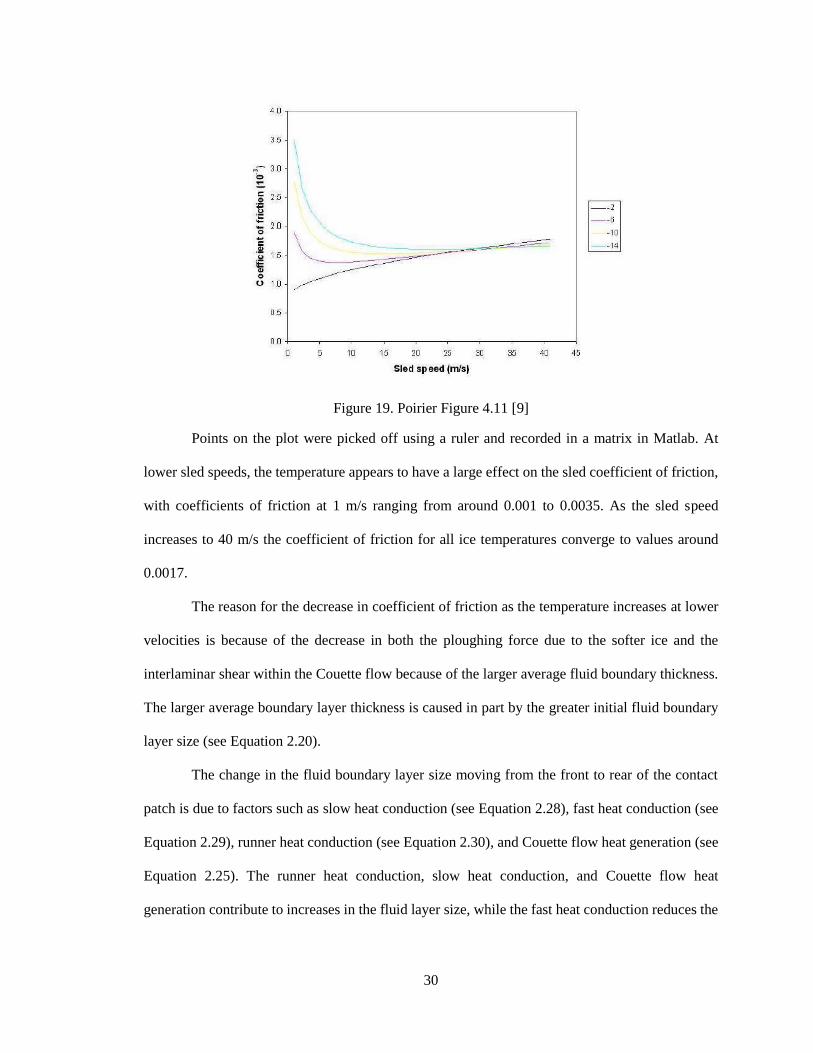
Points on the plot were picked off using a ruler and recorded in a matrix in Matlab. At

lower sled speeds, the temperature appears to have a large effect on the sled coefficient of friction,

with coefficients of friction at 1 m/s ranging from around 0.001 to 0.0035. As the sled speed

increases to 40 m/s the coefficient of friction for all ice temperatures converge to values around

0.0017.

The reason for the decrease in coefficient of friction as the temperature increases at lower

velocities is because of the decrease in both the ploughing force due to the softer ice and the

interlaminar shear within the Couette flow because of the larger average fluid boundary thickness.

The larger average boundary layer thickness is caused in part by the greater initial fluid boundary

layer size (see Equation 2.20).

The change in the fluid boundary layer size moving from the front to rear of the contact

patch is due to factors such as slow heat conduction (see Equation 2.28), fast heat conduction (see

Equation 2.29), runner heat conduction (see Equation 2.30), and Couette flow heat generation (see

Equation 2.25). The runner heat conduction, slow heat conduction, and Couette flow heat

generation contribute to increases in the fluid layer size, while the fast heat conduction reduces the

31

fluid layer size. It is important to note that increases in average fluid layer size result in decreases

in the friction from the Couette flow, while a thinner fluid layer leads to the opposite.

For lower sled velocities, the change in size of the fluid layer along the length of the contact

patch is most effected by the change in fluid layer size from the fast, slow, and runner heat

conduction terms (see Equation 2.32). As the sled velocity is increased, the effect of the Couette

flow heat generation becomes the dominant factor because the value includes a velocity term,

compared to one divided by velocity squared and one divided by velocity for the other terms. For

this reason, at larger sled velocities each constant temperature curve has a gradual, positive slope.

At colder ice temperatures, the magnitude of the temperature difference term outside of the

term including one divided by the square root of velocity in the fast heat conduction portion of the

fluid layer height change equation is much greater. At lower velocities and temperatures the fast

conduction becomes the dominating term, meaning that it will have the greatest influence on the

shape of the coefficient of friction plot. Since the shape of the coefficient of friction plot is inversely

related to the fluid layer height, at lower velocities the lines of colder temperature take the form of

a downward sloping, concave up shape.

At warmer ice temperatures and low velocities, the effect of the fast heat conduction term

is greatly reduced and the slow and runner conduction components of the fluid layer height equation

become the dominating factors. The inverse relationship of the fluid layer height equation to the

coefficient of friction results in a plot with a positive sloping, concave down shape.

32

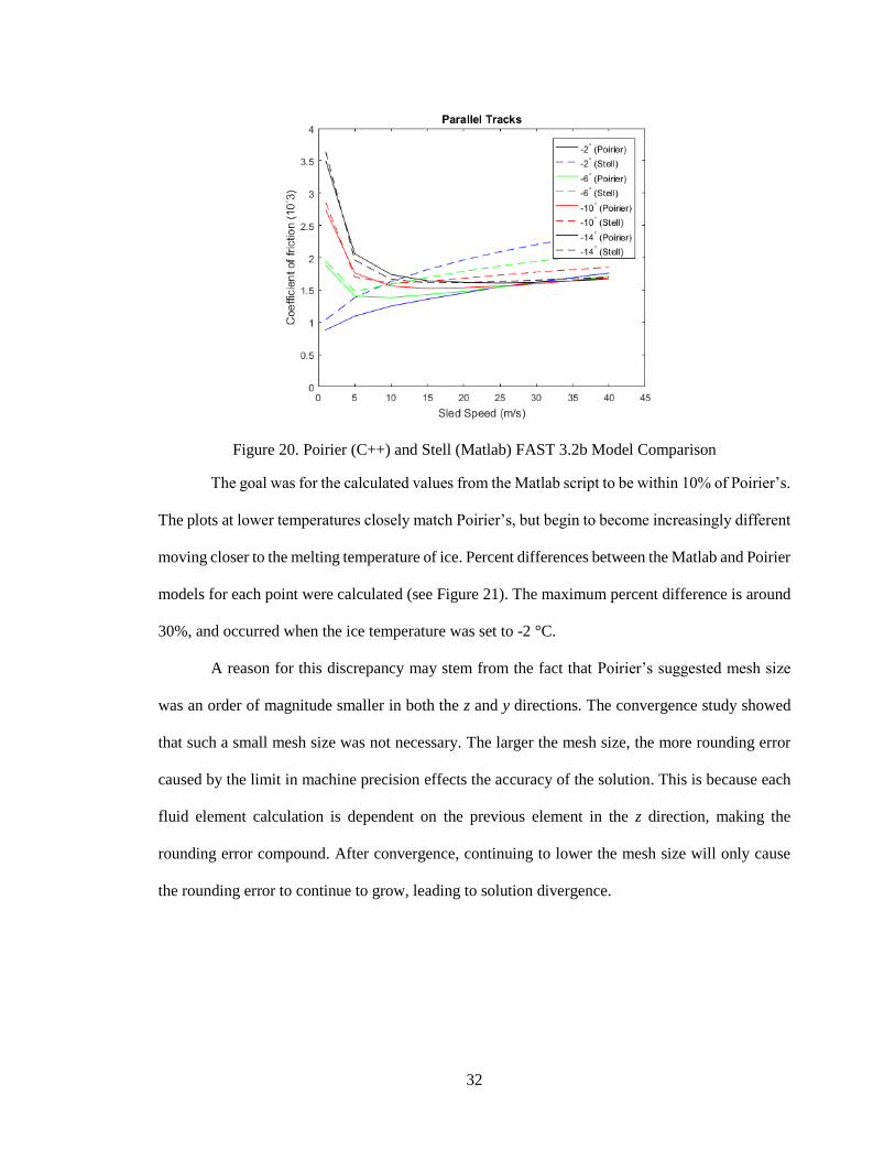
Figure 20. Poirier (C++) and Stell (Matlab) FAST 3.2b Model Comparison

The goal was for the calculated values from the Matlab script to be within 10% of Poirier’s.

The plots at lower temperatures closely match Poirier’s, but begin to become increasingly different

moving closer to the melting temperature of ice. Percent differences between the Matlab and Poirier

models for each point were calculated (see Figure 21). The maximum percent difference is around

30%, and occurred when the ice temperature was set to -2 °C.

A reason for this discrepancy may stem from the fact that Poirier’s suggested mesh size

was an order of magnitude smaller in both the z and y directions. The convergence study showed

that such a small mesh size was not necessary. The larger the mesh size, the more rounding error

caused by the limit in machine precision effects the accuracy of the solution. This is because each

fluid element calculation is dependent on the previous element in the z direction, making the

rounding error compound. After convergence, continuing to lower the mesh size will only cause

the rounding error to continue to grow, leading to solution divergence.

33

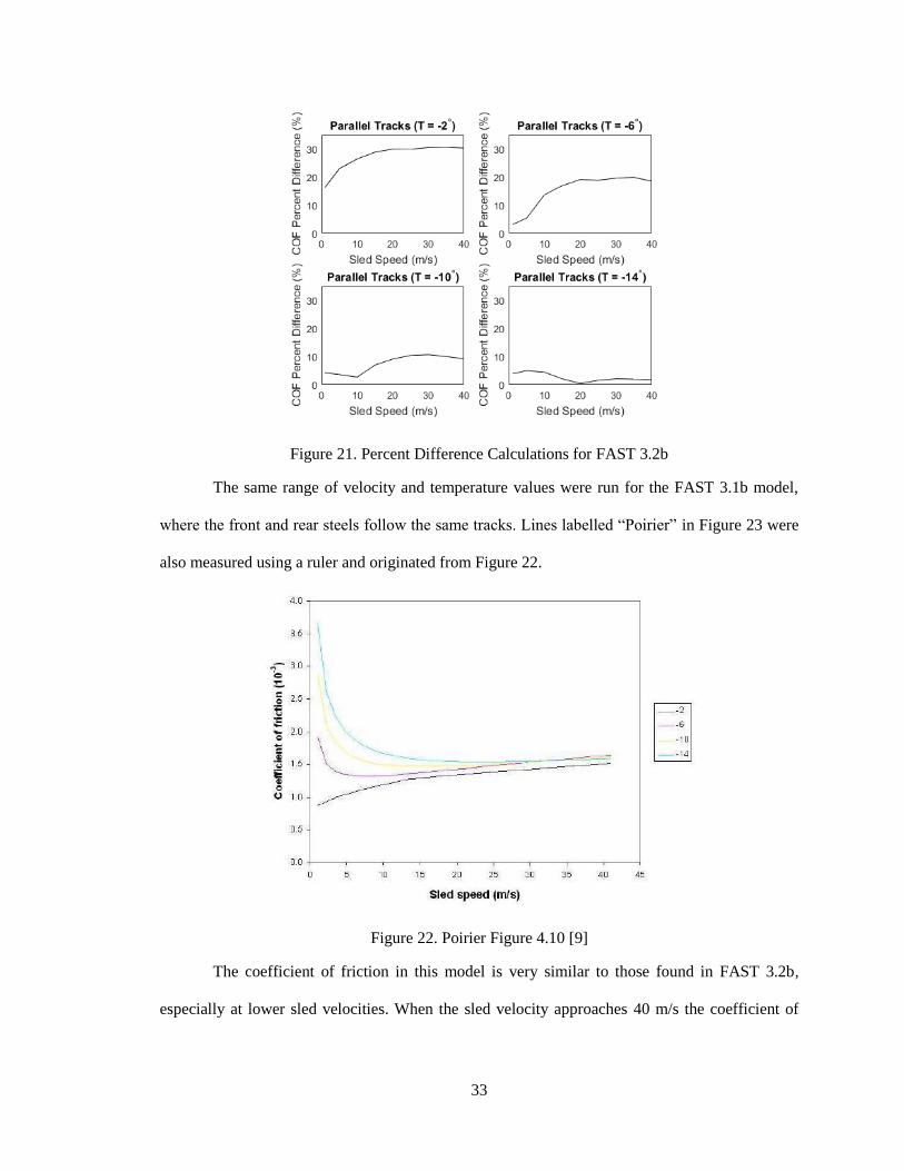
Figure 21. Percent Difference Calculations for FAST 3.2b

The same range of velocity and temperature values were run for the FAST 3.1b model,

where the front and rear steels follow the same tracks. Lines labelled “Poirier” in Figure 23 were

also measured using a ruler and originated from Figure 22.

Figure 22. Poirier Figure 4.10 [9]

The coefficient of friction in this model is very similar to those found in FAST 3.2b,

especially at lower sled velocities. When the sled velocity approaches 40 m/s the coefficient of

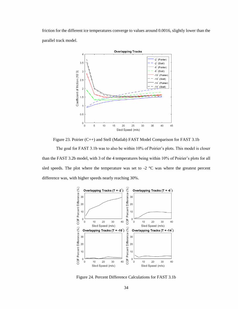
34

friction for the different ice temperatures converge to values around 0.0016, slightly lower than the

parallel track model.

Figure 23. Poirier (C++) and Stell (Matlab) FAST Model Comparison for FAST 3.1b

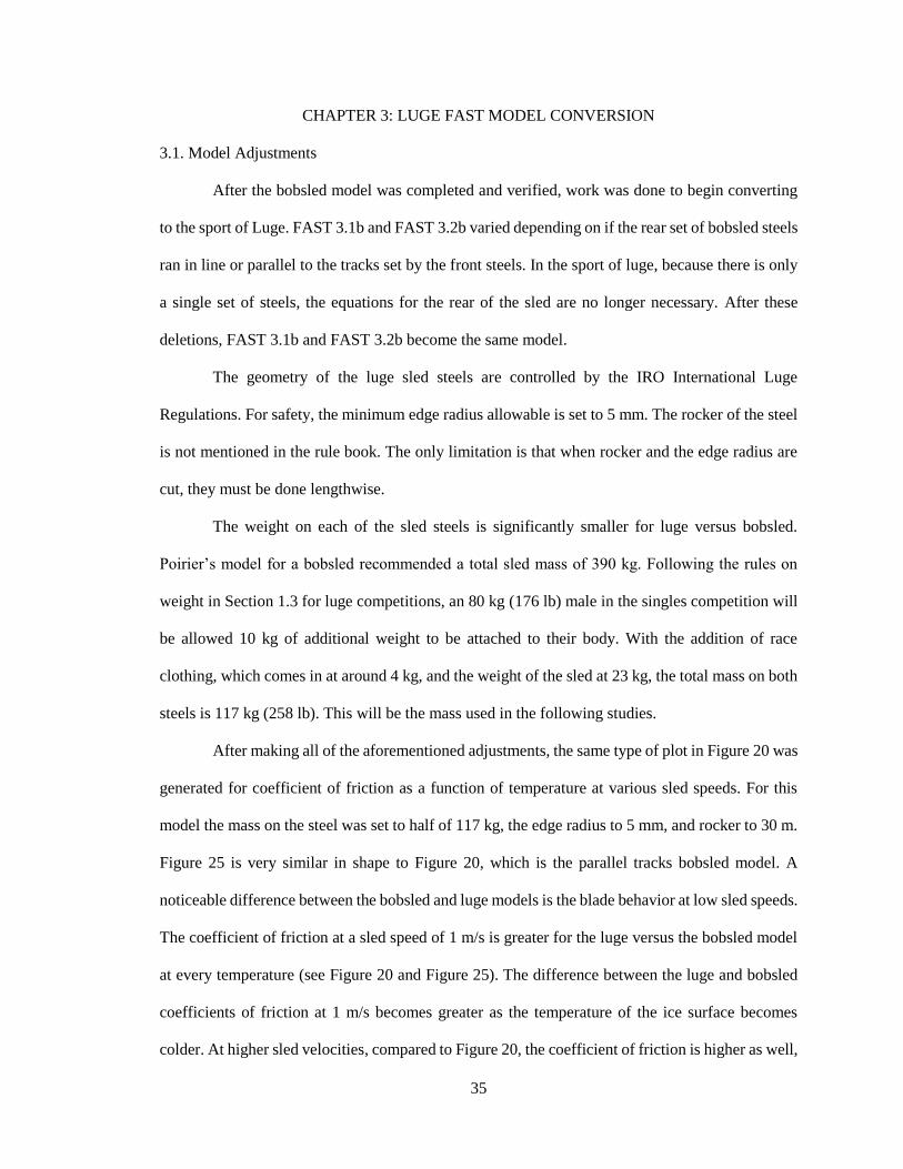
The goal for FAST 3.1b was to also be within 10% of Poirier’s plots. This model is closer

than the FAST 3.2b model, with 3 of the 4 temperatures being within 10% of Poirier’s plots for all

sled speeds. The plot where the temperature was set to -2 °C was where the greatest percent

difference was, with higher speeds nearly reaching 30%.

Figure 24. Percent Difference Calculations for FAST 3.1b

35

CHAPTER 3: LUGE FAST MODEL CONVERSION

3.1. Model Adjustments

After the bobsled model was completed and verified, work was done to begin converting

to the sport of Luge. FAST 3.1b and FAST 3.2b varied depending on if the rear set of bobsled steels

ran in line or parallel to the tracks set by the front steels. In the sport of luge, because there is only

a single set of steels, the equations for the rear of the sled are no longer necessary. After these

deletions, FAST 3.1b and FAST 3.2b become the same model.

The geometry of the luge sled steels are controlled by the IRO International Luge

Regulations. For safety, the minimum edge radius allowable is set to 5 mm. The rocker of the steel

is not mentioned in the rule book. The only limitation is that when rocker and the edge radius are

cut, they must be done lengthwise.

The weight on each of the sled steels is significantly smaller for luge versus bobsled.

Poirier’s model for a bobsled recommended a total sled mass of 390 kg. Following the rules on

weight in Section 1.3 for luge competitions, an 80 kg (176 lb) male in the singles competition will

be allowed 10 kg of additional weight to be attached to their body. With the addition of race

clothing, which comes in at around 4 kg, and the weight of the sled at 23 kg, the total mass on both

steels is 117 kg (258 lb). This will be the mass used in the following studies.

After making all of the aforementioned adjustments, the same type of plot in Figure 20 was

generated for coefficient of friction as a function of temperature at various sled speeds. For this

model the mass on the steel was set to half of 117 kg, the edge radius to 5 mm, and rocker to 30 m.

Figure 25 is very similar in shape to Figure 20, which is the parallel tracks bobsled model. A

noticeable difference between the bobsled and luge models is the blade behavior at low sled speeds.

The coefficient of friction at a sled speed of 1 m/s is greater for the luge versus the bobsled model

at every temperature (see Figure 20 and Figure 25). The difference between the luge and bobsled

coefficients of friction at 1 m/s becomes greater as the temperature of the ice surface becomes

colder. At higher sled velocities, compared to Figure 20, the coefficient of friction is higher as well,

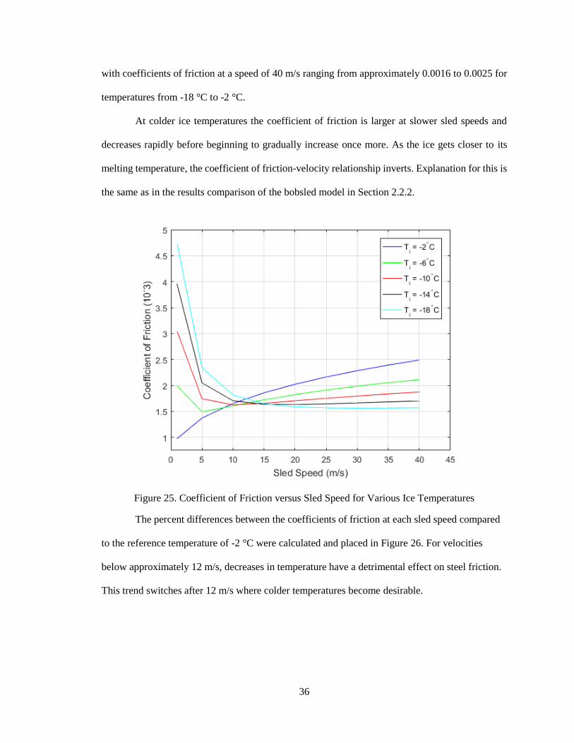
36

with coefficients of friction at a speed of 40 m/s ranging from approximately 0.0016 to 0.0025 for

temperatures from -18 °C to -2 °C.

At colder ice temperatures the coefficient of friction is larger at slower sled speeds and

decreases rapidly before beginning to gradually increase once more. As the ice gets closer to its

melting temperature, the coefficient of friction-velocity relationship inverts. Explanation for this is

the same as in the results comparison of the bobsled model in Section 2.2.2.

Figure 25. Coefficient of Friction versus Sled Speed for Various Ice Temperatures

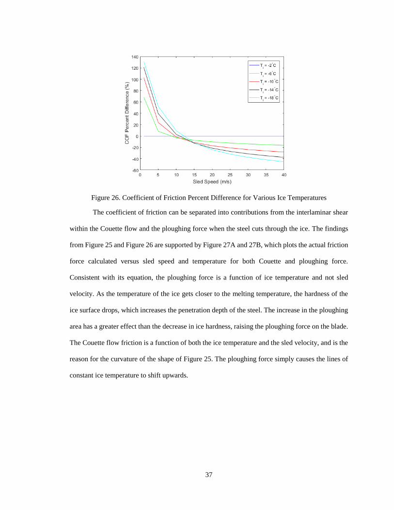
The percent differences between the coefficients of friction at each sled speed compared

to the reference temperature of -2 °C were calculated and placed in Figure 26. For velocities

below approximately 12 m/s, decreases in temperature have a detrimental effect on steel friction.

This trend switches after 12 m/s where colder temperatures become desirable.

37

Figure 26. Coefficient of Friction Percent Difference for Various Ice Temperatures

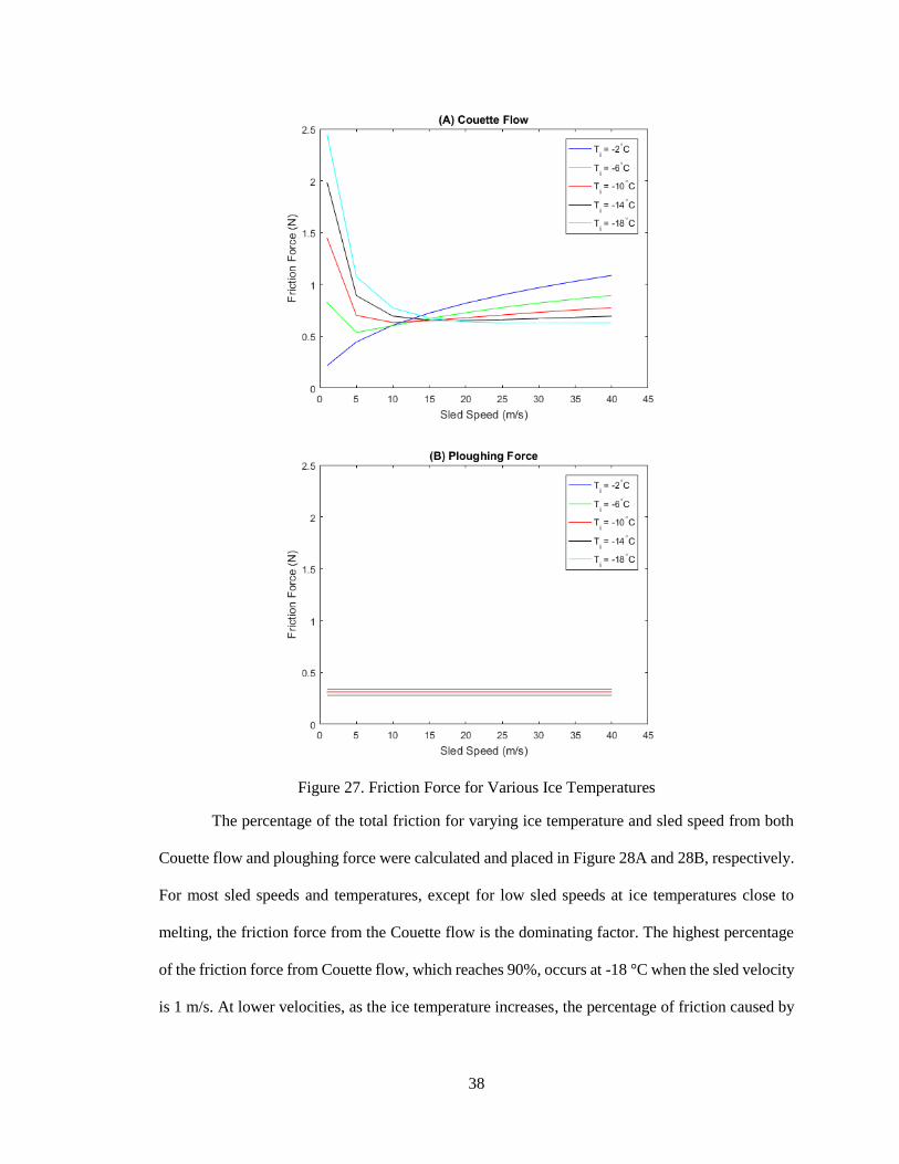
The coefficient of friction can be separated into contributions from the interlaminar shear

within the Couette flow and the ploughing force when the steel cuts through the ice. The findings

from Figure 25 and Figure 26 are supported by Figure 27A and 27B, which plots the actual friction

force calculated versus sled speed and temperature for both Couette and ploughing force.

Consistent with its equation, the ploughing force is a function of ice temperature and not sled

velocity. As the temperature of the ice gets closer to the melting temperature, the hardness of the

ice surface drops, which increases the penetration depth of the steel. The increase in the ploughing

area has a greater effect than the decrease in ice hardness, raising the ploughing force on the blade.

The Couette flow friction is a function of both the ice temperature and the sled velocity, and is the

reason for the curvature of the shape of Figure 25. The ploughing force simply causes the lines of

constant ice temperature to shift upwards.

38

Figure 27. Friction Force for Various Ice Temperatures

The percentage of the total friction for varying ice temperature and sled speed from both

Couette flow and ploughing force were calculated and placed in Figure 28A and 28B, respectively.

For most sled speeds and temperatures, except for low sled speeds at ice temperatures close to

melting, the friction force from the Couette flow is the dominating factor. The highest percentage

of the friction force from Couette flow, which reaches 90%, occurs at -18 °C when the sled velocity

is 1 m/s. At lower velocities, as the ice temperature increases, the percentage of friction caused by

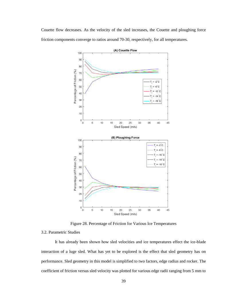
39

Couette flow decreases. As the velocity of the sled increases, the Couette and ploughing force

friction components converge to ratios around 70-30, respectively, for all temperatures.

Figure 28. Percentage of Friction for Various Ice Temperatures

3.2. Parametric Studies

It has already been shown how sled velocities and ice temperatures effect the ice-blade

interaction of a luge sled. What has yet to be explored is the effect that sled geometry has on

performance. Sled geometry in this model is simplified to two factors, edge radius and rocker. The

coefficient of friction versus sled velocity was plotted for various edge radii ranging from 5 mm to

40

14 mm. The mass on the steel was set to half of 117 kg, the ice temperature to -10 °C, and the

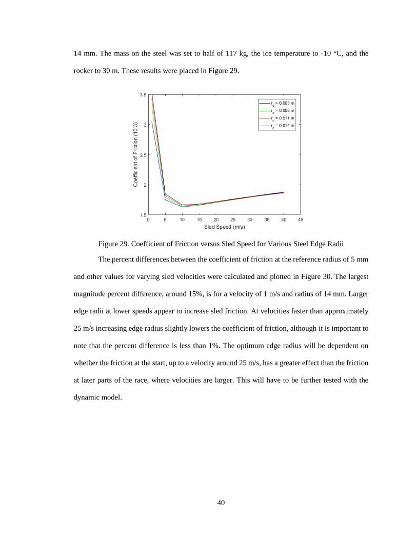
rocker to 30 m. These results were placed in Figure 29.

Figure 29. Coefficient of Friction versus Sled Speed for Various Steel Edge Radii

The percent differences between the coefficient of friction at the reference radius of 5 mm

and other values for varying sled velocities were calculated and plotted in Figure 30. The largest

magnitude percent difference, around 15%, is for a velocity of 1 m/s and radius of 14 mm. Larger

edge radii at lower speeds appear to increase sled friction. At velocities faster than approximately

25 m/s increasing edge radius slightly lowers the coefficient of friction, although it is important to

note that the percent difference is less than 1%. The optimum edge radius will be dependent on

whether the friction at the start, up to a velocity around 25 m/s, has a greater effect than the friction

at later parts of the race, where velocities are larger. This will have to be further tested with the

dynamic model.

41

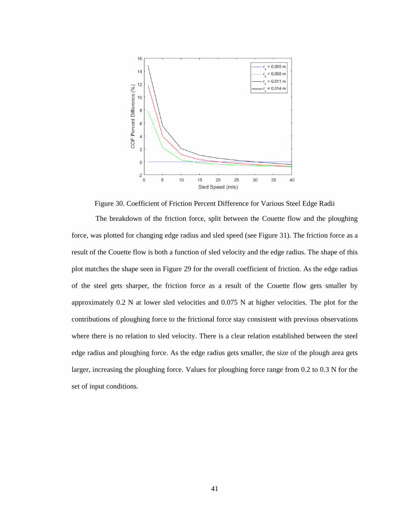
Figure 30. Coefficient of Friction Percent Difference for Various Steel Edge Radii

The breakdown of the friction force, split between the Couette flow and the ploughing

force, was plotted for changing edge radius and sled speed (see Figure 31). The friction force as a

result of the Couette flow is both a function of sled velocity and the edge radius. The shape of this

plot matches the shape seen in Figure 29 for the overall coefficient of friction. As the edge radius

of the steel gets sharper, the friction force as a result of the Couette flow gets smaller by

approximately 0.2 N at lower sled velocities and 0.075 N at higher velocities. The plot for the

contributions of ploughing force to the frictional force stay consistent with previous observations

where there is no relation to sled velocity. There is a clear relation established between the steel

edge radius and ploughing force. As the edge radius gets smaller, the size of the plough area gets

larger, increasing the ploughing force. Values for ploughing force range from 0.2 to 0.3 N for the

set of input conditions.

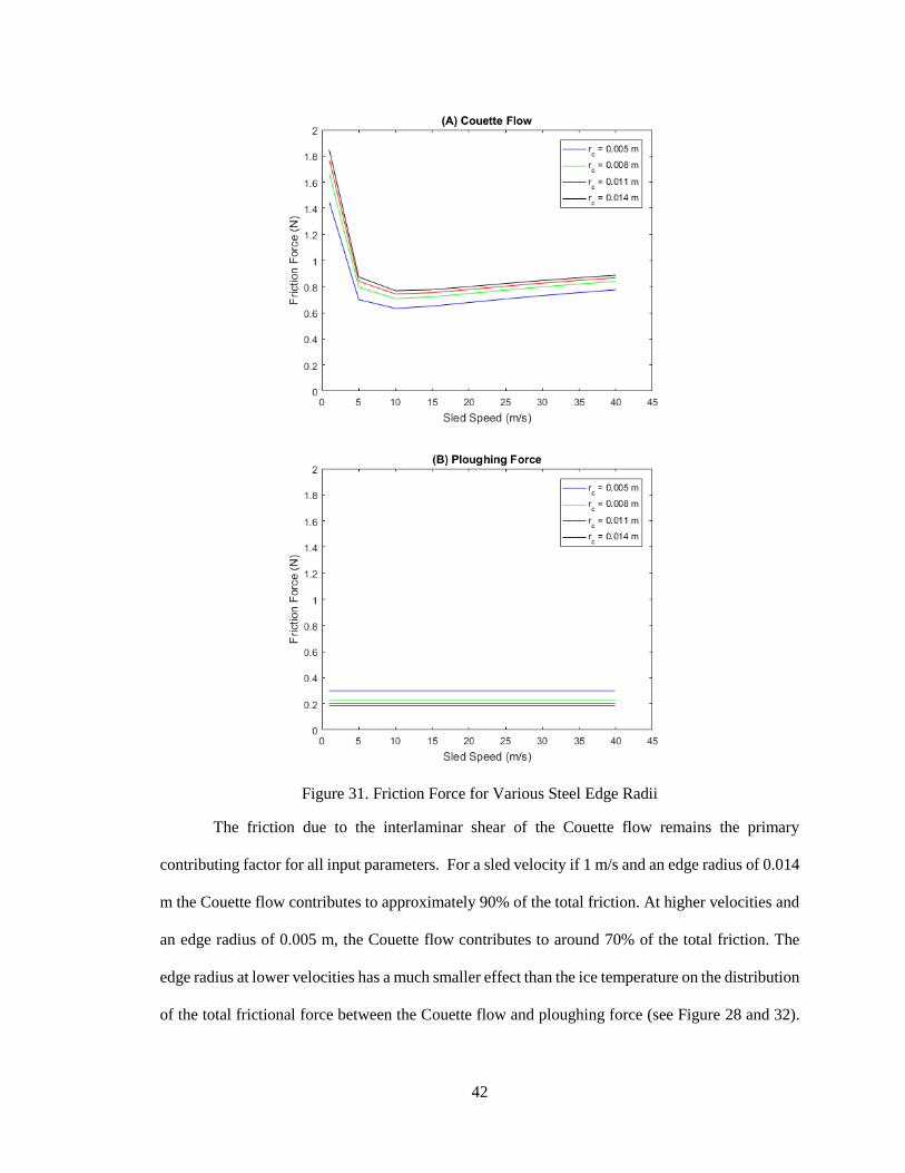
42

Figure 31. Friction Force for Various Steel Edge Radii

The friction due to the interlaminar shear of the Couette flow remains the primary

contributing factor for all input parameters. For a sled velocity if 1 m/s and an edge radius of 0.014

m the Couette flow contributes to approximately 90% of the total friction. At higher velocities and

an edge radius of 0.005 m, the Couette flow contributes to around 70% of the total friction. The

edge radius at lower velocities has a much smaller effect than the ice temperature on the distribution

of the total frictional force between the Couette flow and ploughing force (see Figure 28 and 32).

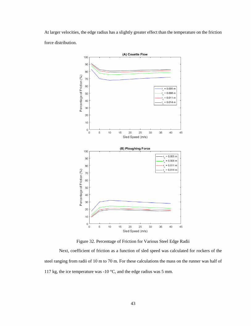
43

At larger velocities, the edge radius has a slightly greater effect than the temperature on the friction

force distribution.

Figure 32. Percentage of Friction for Various Steel Edge Radii

Next, coefficient of friction as a function of sled speed was calculated for rockers of the

steel ranging from radii of 10 m to 70 m. For these calculations the mass on the runner was half of

117 kg, the ice temperature was -10 °C, and the edge radius was 5 mm.

44

Figure 33. Coefficient of Friction versus Sled Speed for Various Rockers

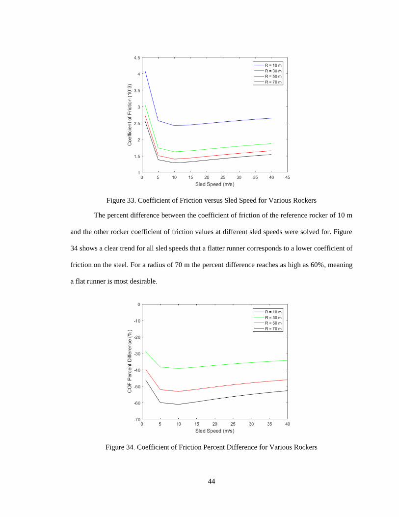
The percent difference between the coefficient of friction of the reference rocker of 10 m

and the other rocker coefficient of friction values at different sled speeds were solved for. Figure

34 shows a clear trend for all sled speeds that a flatter runner corresponds to a lower coefficient of

friction on the steel. For a radius of 70 m the percent difference reaches as high as 60%, meaning

a flat runner is most desirable.

Figure 34. Coefficient of Friction Percent Difference for Various Rockers

45

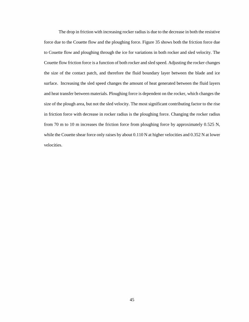
The drop in friction with increasing rocker radius is due to the decrease in both the resistive

force due to the Couette flow and the ploughing force. Figure 35 shows both the friction force due

to Couette flow and ploughing through the ice for variations in both rocker and sled velocity. The

Couette flow friction force is a function of both rocker and sled speed. Adjusting the rocker changes

the size of the contact patch, and therefore the fluid boundary layer between the blade and ice

surface. Increasing the sled speed changes the amount of heat generated between the fluid layers

and heat transfer between materials. Ploughing force is dependent on the rocker, which changes the

size of the plough area, but not the sled velocity. The most significant contributing factor to the rise

in friction force with decrease in rocker radius is the ploughing force. Changing the rocker radius

from 70 m to 10 m increases the friction force from ploughing force by approximately 0.525 N,

while the Couette shear force only raises by about 0.110 N at higher velocities and 0.352 N at lower

velocities.

46

Figure 35. Friction Force for Various Rockers

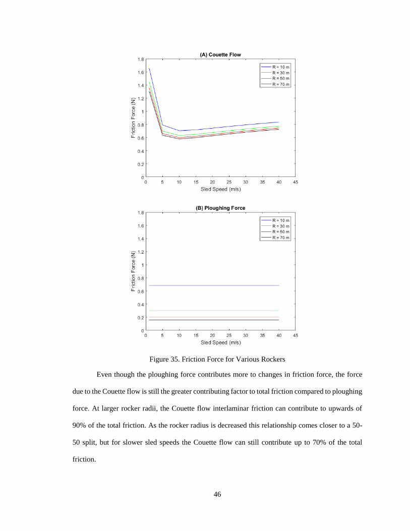
Even though the ploughing force contributes more to changes in friction force, the force

due to the Couette flow is still the greater contributing factor to total friction compared to ploughing

force. At larger rocker radii, the Couette flow interlaminar friction can contribute to upwards of

90% of the total friction. As the rocker radius is decreased this relationship comes closer to a 50-

50 split, but for slower sled speeds the Couette flow can still contribute up to 70% of the total

friction.

47

Figure 36. Percentage of Friction for Various Rockers

3.3 Banked Curves

The luge model converted from FAST 3.1b and FAST 3.2b does not include how a banked

curve effects the friction on a sled steel. Depending on the velocity of the sled going into the curve

and the curve geometry, the coefficient of friction has the potential to change.

3.3.1. Weight Change

One of the factors leading to differences in the size of the contact patch and therefore the

friction coefficient is the loading on the sled when going around a banked curve. Riders and their

48

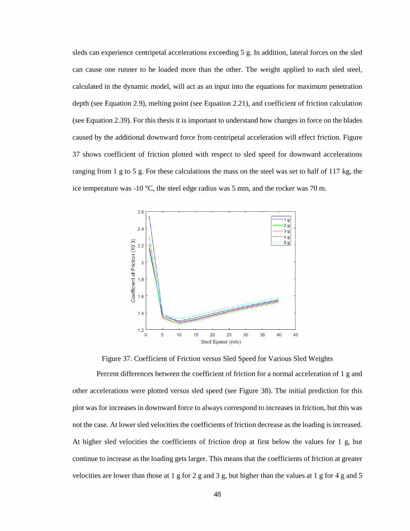
sleds can experience centripetal accelerations exceeding 5 g. In addition, lateral forces on the sled

can cause one runner to be loaded more than the other. The weight applied to each sled steel,

calculated in the dynamic model, will act as an input into the equations for maximum penetration

depth (see Equation 2.9), melting point (see Equation 2.21), and coefficient of friction calculation

(see Equation 2.39). For this thesis it is important to understand how changes in force on the blades

caused by the additional downward force from centripetal acceleration will effect friction. Figure

37 shows coefficient of friction plotted with respect to sled speed for downward accelerations

ranging from 1 g to 5 g. For these calculations the mass on the steel was set to half of 117 kg, the

ice temperature was -10 °C, the steel edge radius was 5 mm, and the rocker was 70 m.

Figure 37. Coefficient of Friction versus Sled Speed for Various Sled Weights

Percent differences between the coefficient of friction for a normal acceleration of 1 g and

other accelerations were plotted versus sled speed (see Figure 38). The initial prediction for this

plot was for increases in downward force to always correspond to increases in friction, but this was

not the case. At lower sled velocities the coefficients of friction decrease as the loading is increased.

At higher sled velocities the coefficients of friction drop at first below the values for 1 g, but

continue to increase as the loading gets larger. This means that the coefficients of friction at greater

velocities are lower than those at 1 g for 2 g and 3 g, but higher than the values at 1 g for 4 g and 5

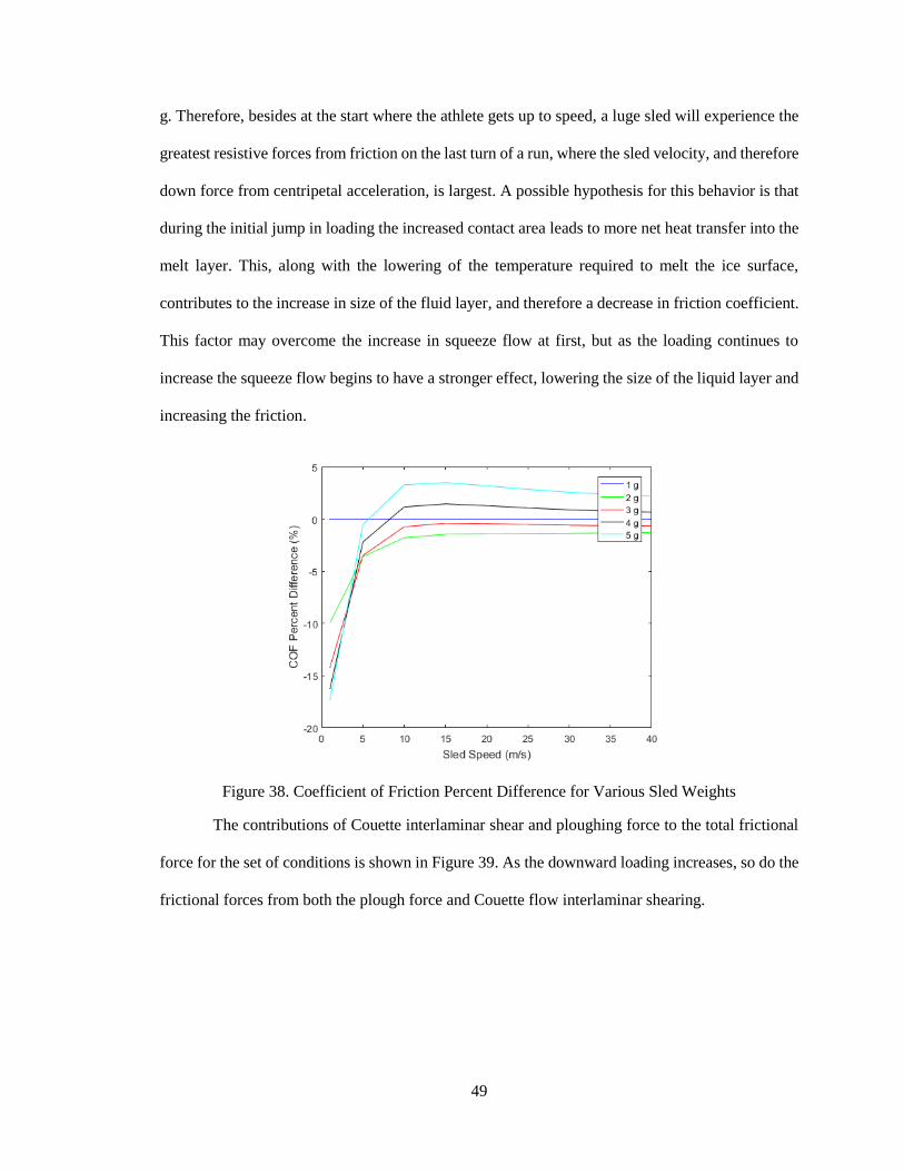
49

g. Therefore, besides at the start where the athlete gets up to speed, a luge sled will experience the

greatest resistive forces from friction on the last turn of a run, where the sled velocity, and therefore

down force from centripetal acceleration, is largest. A possible hypothesis for this behavior is that

during the initial jump in loading the increased contact area leads to more net heat transfer into the

melt layer. This, along with the lowering of the temperature required to melt the ice surface,

contributes to the increase in size of the fluid layer, and therefore a decrease in friction coefficient.

This factor may overcome the increase in squeeze flow at first, but as the loading continues to

increase the squeeze flow begins to have a stronger effect, lowering the size of the liquid layer and

increasing the friction.

Figure 38. Coefficient of Friction Percent Difference for Various Sled Weights

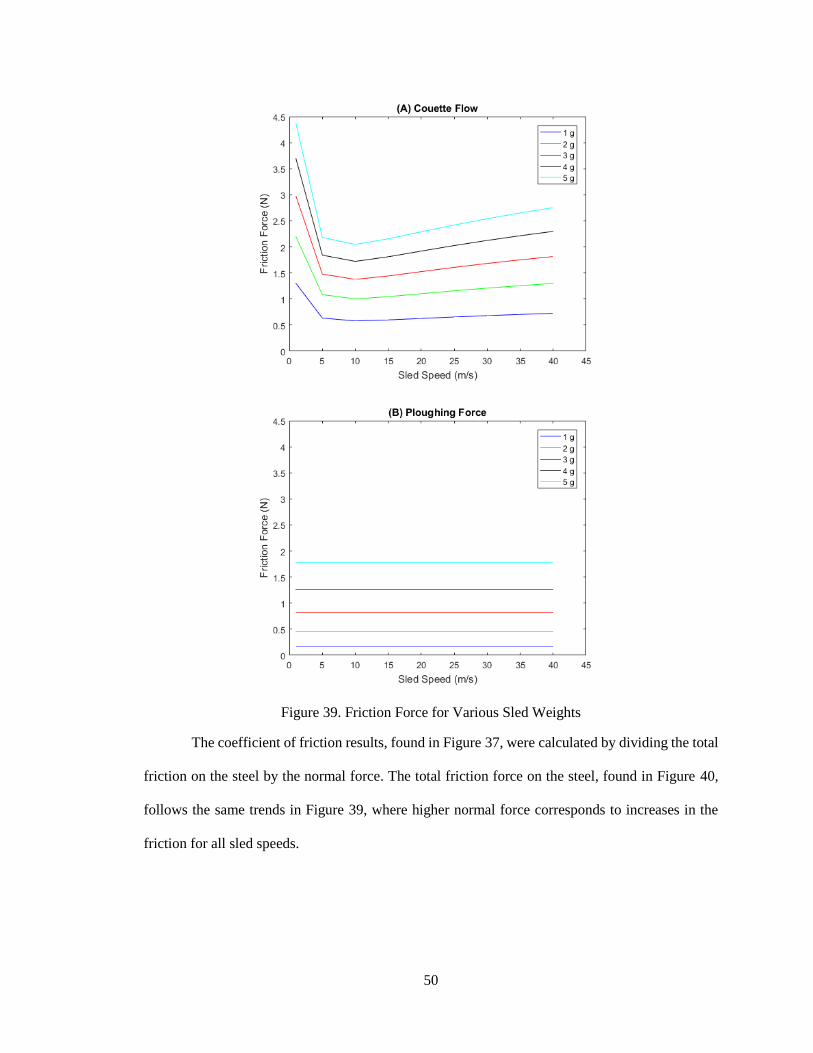
The contributions of Couette interlaminar shear and ploughing force to the total frictional

force for the set of conditions is shown in Figure 39. As the downward loading increases, so do the

frictional forces from both the plough force and Couette flow interlaminar shearing.

50

Figure 39. Friction Force for Various Sled Weights

The coefficient of friction results, found in Figure 37, were calculated by dividing the total

friction on the steel by the normal force. The total friction force on the steel, found in Figure 40,

follows the same trends in Figure 39, where higher normal force corresponds to increases in the

friction for all sled speeds.

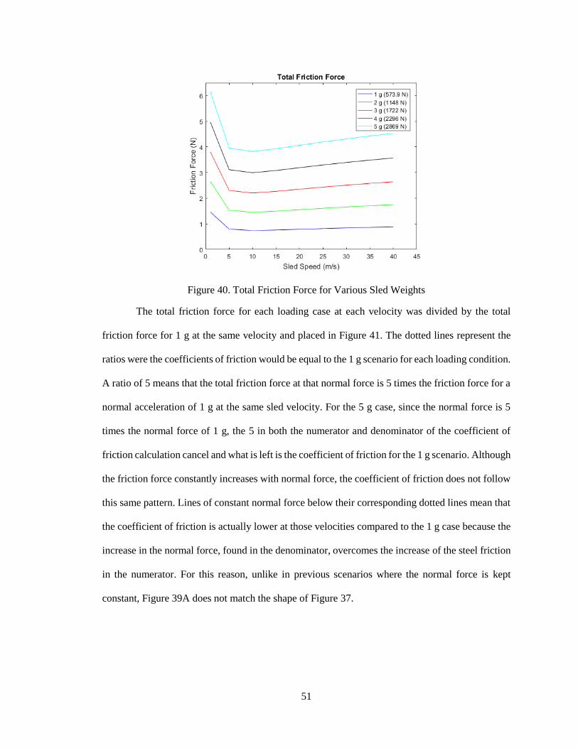
51

Figure 40. Total Friction Force for Various Sled Weights

The total friction force for each loading case at each velocity was divided by the total

friction force for 1 g at the same velocity and placed in Figure 41. The dotted lines represent the

ratios were the coefficients of friction would be equal to the 1 g scenario for each loading condition.

A ratio of 5 means that the total friction force at that normal force is 5 times the friction force for a

normal acceleration of 1 g at the same sled velocity. For the 5 g case, since the normal force is 5

times the normal force of 1 g, the 5 in both the numerator and denominator of the coefficient of

friction calculation cancel and what is left is the coefficient of friction for the 1 g scenario. Although

the friction force constantly increases with normal force, the coefficient of friction does not follow

this same pattern. Lines of constant normal force below their corresponding dotted lines mean that

the coefficient of friction is actually lower at those velocities compared to the 1 g case because the

increase in the normal force, found in the denominator, overcomes the increase of the steel friction

in the numerator. For this reason, unlike in previous scenarios where the normal force is kept

constant, Figure 39A does not match the shape of Figure 37.

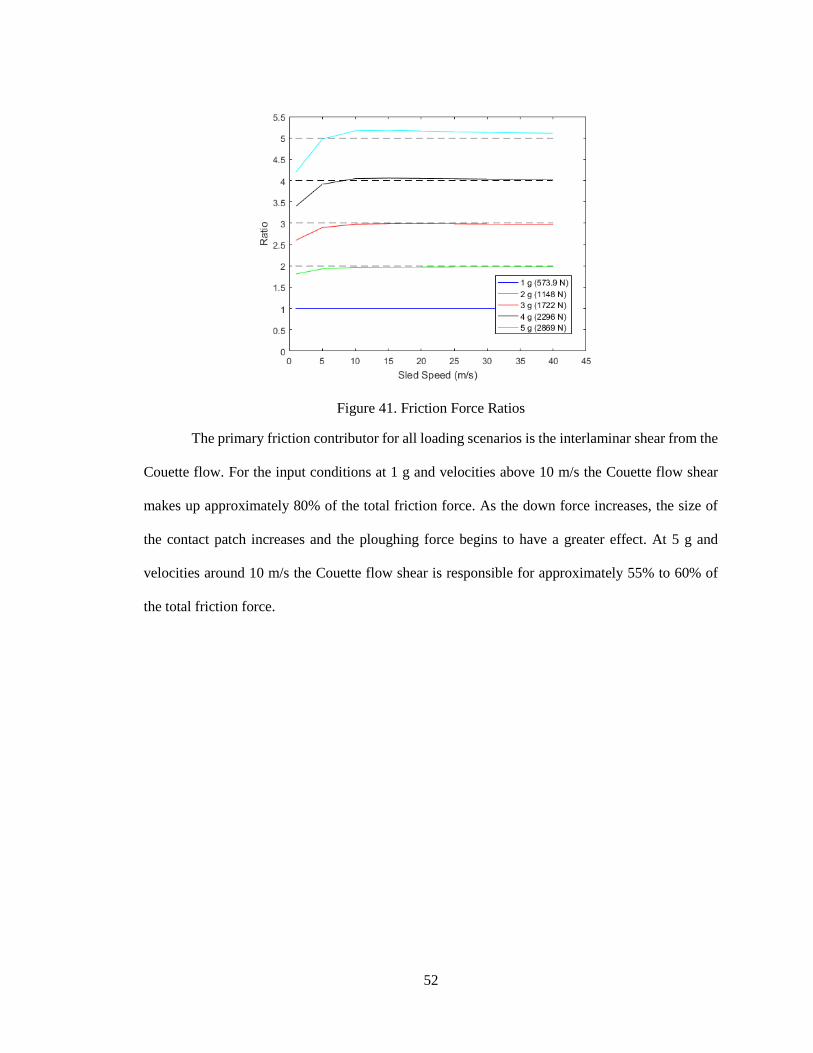
52

Figure 41. Friction Force Ratios

The primary friction contributor for all loading scenarios is the interlaminar shear from the

Couette flow. For the input conditions at 1 g and velocities above 10 m/s the Couette flow shear

makes up approximately 80% of the total friction force. As the down force increases, the size of

the contact patch increases and the ploughing force begins to have a greater effect. At 5 g and

velocities around 10 m/s the Couette flow shear is responsible for approximately 55% to 60% of

the total friction force.

53

Figure 42. Percentage of Friction for Various Sled Weights

3.3.2. Side Slip

Moving into the banked section of the track introduces the inclusion of lateral forces on

the sled. There are limitations to the amount of side force that the ice surface can handle before it

gives way to the lateral movement of the blade. Lateral ploughing of the ice surface causes the sled

to veer off of its optimum line, having a detrimental effect on run times. It also leads to a spike in

the ploughing force contributing to the friction between the steel and ice surface. For these reasons,

avoiding any side slip of the blade is of utmost importance on turns. The equation for the allowable

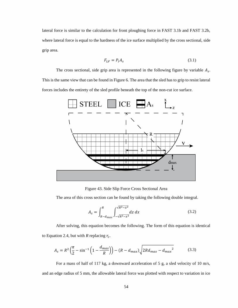
54

lateral force is similar to the calculation for front ploughing force in FAST 3.1b and FAST 3.2b,

where lateral force is equal to the hardness of the ice surface multiplied by the cross sectional, side

grip area.

𝐹𝐿𝐹 = 𝑃𝐼𝐴𝑠 (3.1)

The cross sectional, side grip area is represented in the following figure by variable 𝐴𝑠.

This is the same view that can be found in Figure 6. The area that the sled has to grip to resist lateral

forces includes the entirety of the sled profile beneath the top of the non-cut ice surface.

Figure 43. Side Slip Force Cross Sectional Area

The area of this cross section can be found by taking the following double integral.

𝐴𝑠 = ∫ ∫ 𝑑𝑧 𝑑𝑥√𝑅2−𝑥2

−√𝑅2−𝑥2

𝑅

𝑅−𝑑𝑚𝑎𝑥

(3.2)

After solving, this equation becomes the following. The form of this equation is identical

to Equation 2.4, but with R replacing 𝑟𝑐.

𝐴𝑠 = 𝑅2 (𝜋

2− sin−1 (1 −

𝑑𝑚𝑎𝑥

𝑅)) − (𝑅 − 𝑑𝑚𝑎𝑥)√2𝑅𝑑𝑚𝑎𝑥 − 𝑑𝑚𝑎𝑥

2 (3.3)

For a mass of half of 117 kg, a downward acceleration of 5 g, a sled velocity of 10 m/s,

and an edge radius of 5 mm, the allowable lateral force was plotted with respect to variation in ice

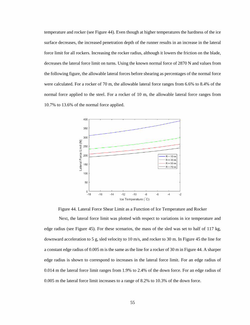
55

temperature and rocker (see Figure 44). Even though at higher temperatures the hardness of the ice

surface decreases, the increased penetration depth of the runner results in an increase in the lateral

force limit for all rockers. Increasing the rocker radius, although it lowers the friction on the blade,

decreases the lateral force limit on turns. Using the known normal force of 2870 N and values from

the following figure, the allowable lateral forces before shearing as percentages of the normal force

were calculated. For a rocker of 70 m, the allowable lateral force ranges from 6.6% to 8.4% of the

normal force applied to the steel. For a rocker of 10 m, the allowable lateral force ranges from

10.7% to 13.6% of the normal force applied.

Figure 44. Lateral Force Shear Limit as a Function of Ice Temperature and Rocker

Next, the lateral force limit was plotted with respect to variations in ice temperature and

edge radius (see Figure 45). For these scenarios, the mass of the sled was set to half of 117 kg,

downward acceleration to 5 g, sled velocity to 10 m/s, and rocker to 30 m. In Figure 45 the line for

a constant edge radius of 0.005 m is the same as the line for a rocker of 30 m in Figure 44. A sharper

edge radius is shown to correspond to increases in the lateral force limit. For an edge radius of

0.014 m the lateral force limit ranges from 1.9% to 2.4% of the down force. For an edge radius of

0.005 m the lateral force limit increases to a range of 8.2% to 10.3% of the down force.

56

Figure 45. Lateral Force Limit as a Function of Ice Temperature and Edge Radius

The effect of normal loading on the allowable lateral force was plotted for downward

accelerations from 1 g to 5 g (see Figure 46). For this analysis the mass of the sled was set to half

of 117 kg, sled velocity was set to 10 m/s, the edge radius to 5 mm, and the rocker to 70 m. A clear

increase in the lateral force limit is shown as the downward acceleration of the sled mass goes from

1 g to 5 g. The lateral force limits for varying ice temperature and a loading of 5 g are approximately

11.2 times greater than the corresponding force limits seen for loading of 1 g.

Figure 46. Lateral Force Limit as a Function of Ice Temperature and Down Force

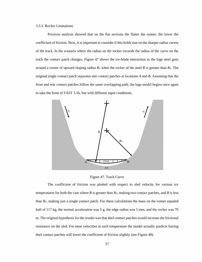
57

3.3.3. Rocker Limitations

Previous analysis showed that on the flat sections the flatter the runner, the lower the

coefficient of friction. Next, it is important to consider if this holds true on the sharper radius curves

of the track. In the scenario where the radius on the rocker exceeds the radius of the curve on the

track the contact patch changes. Figure 47 shows the ice-blade interaction as the luge steel goes

around a corner of upward sloping radius RT when the rocker of the steel R is greater than RT. The

original single contact patch separates into contact patches at locations A and B. Assuming that the

front and rear contact patches follow the same overlapping path, the luge model begins once again

to take the form of FAST 3.1b, but with different input conditions.

Figure 47. Track Curve

The coefficient of friction was plotted with respect to sled velocity for various ice

temperatures for both the case where R is greater than RT, making two contact patches, and R is less

than RT, making just a single contact patch. For these calculations the mass on the runner equaled

half of 117 kg, the normal acceleration was 5 g, the edge radius was 5 mm, and the rocker was 70

m. The original hypothesis for the results was that duel contact patches would increase the frictional

resistance on the sled. For most velocities at each temperature the model actually predicts having

duel contact patches will lower the coefficient of friction slightly (see Figure 48).

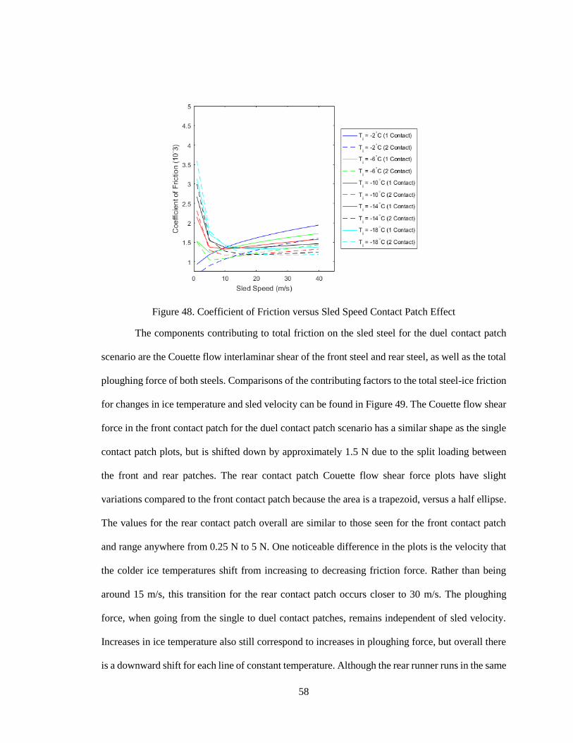
58

Figure 48. Coefficient of Friction versus Sled Speed Contact Patch Effect

The components contributing to total friction on the sled steel for the duel contact patch

scenario are the Couette flow interlaminar shear of the front steel and rear steel, as well as the total

ploughing force of both steels. Comparisons of the contributing factors to the total steel-ice friction

for changes in ice temperature and sled velocity can be found in Figure 49. The Couette flow shear

force in the front contact patch for the duel contact patch scenario has a similar shape as the single

contact patch plots, but is shifted down by approximately 1.5 N due to the split loading between

the front and rear patches. The rear contact patch Couette flow shear force plots have slight

variations compared to the front contact patch because the area is a trapezoid, versus a half ellipse.

The values for the rear contact patch overall are similar to those seen for the front contact patch

and range anywhere from 0.25 N to 5 N. One noticeable difference in the plots is the velocity that

the colder ice temperatures shift from increasing to decreasing friction force. Rather than being

around 15 m/s, this transition for the rear contact patch occurs closer to 30 m/s. The ploughing

force, when going from the single to duel contact patches, remains independent of sled velocity.

Increases in ice temperature also still correspond to increases in ploughing force, but overall there

is a downward shift for each line of constant temperature. Although the rear runner runs in the same

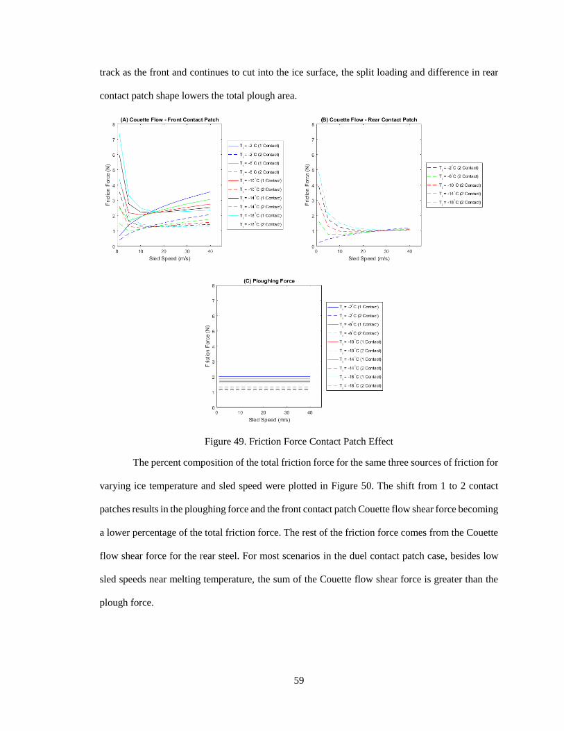
59

track as the front and continues to cut into the ice surface, the split loading and difference in rear

contact patch shape lowers the total plough area.

Figure 49. Friction Force Contact Patch Effect

The percent composition of the total friction force for the same three sources of friction for

varying ice temperature and sled speed were plotted in Figure 50. The shift from 1 to 2 contact

patches results in the ploughing force and the front contact patch Couette flow shear force becoming

a lower percentage of the total friction force. The rest of the friction force comes from the Couette

flow shear force for the rear steel. For most scenarios in the duel contact patch case, besides low

sled speeds near melting temperature, the sum of the Couette flow shear force is greater than the

plough force.

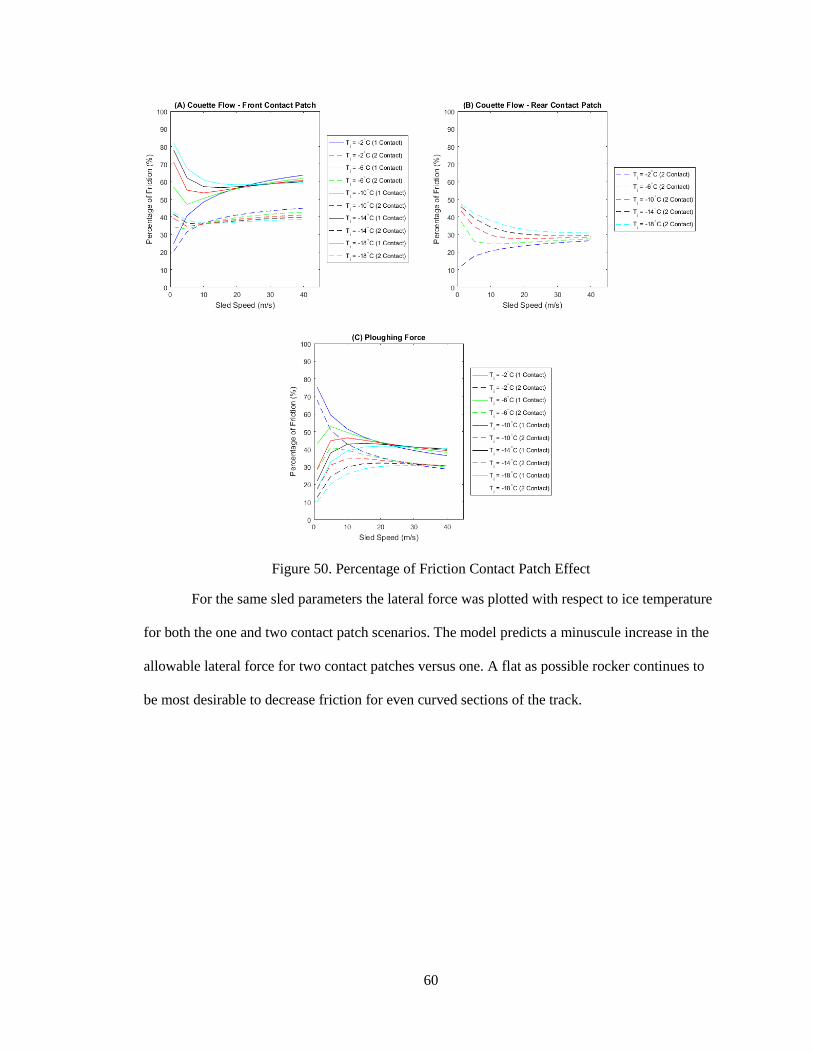
60

Figure 50. Percentage of Friction Contact Patch Effect

For the same sled parameters the lateral force was plotted with respect to ice temperature

for both the one and two contact patch scenarios. The model predicts a minuscule increase in the

allowable lateral force for two contact patches versus one. A flat as possible rocker continues to

be most desirable to decrease friction for even curved sections of the track.

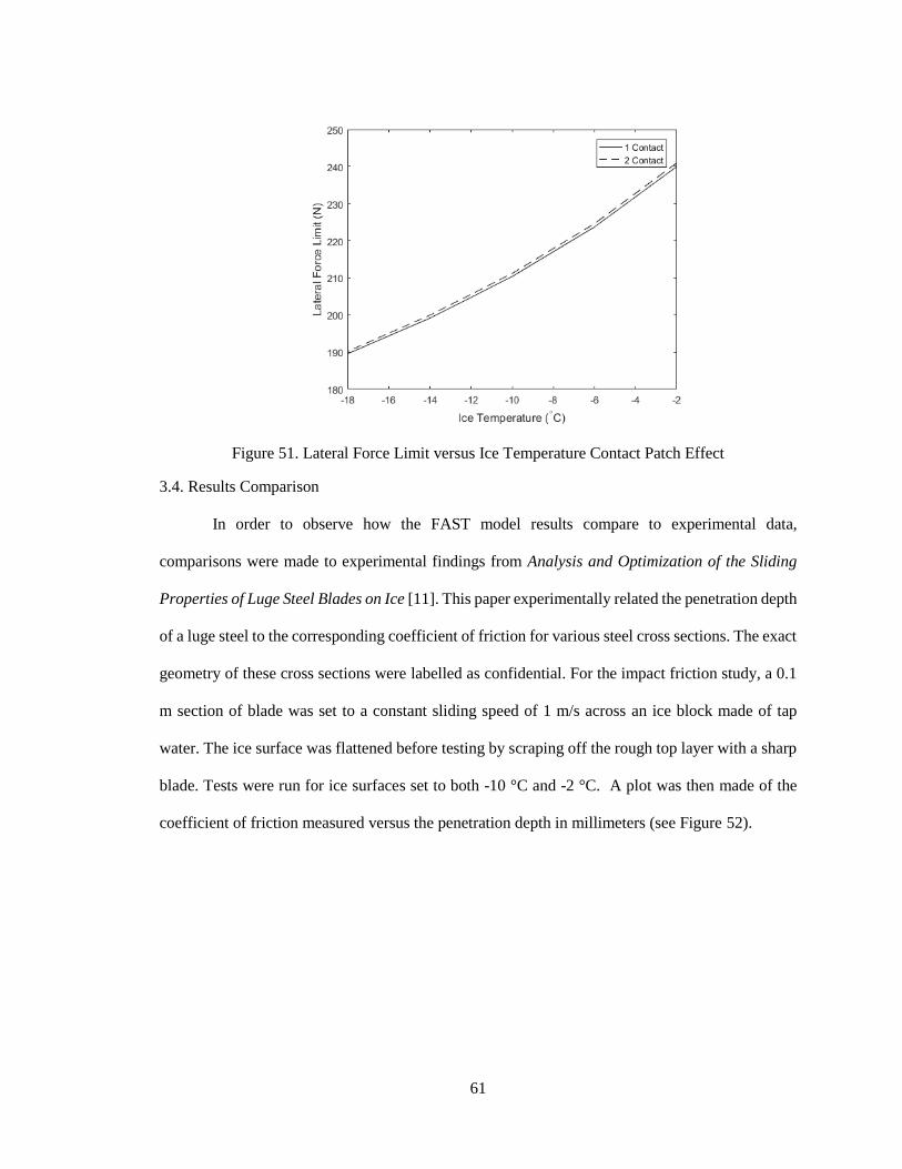
61

Figure 51. Lateral Force Limit versus Ice Temperature Contact Patch Effect

3.4. Results Comparison

In order to observe how the FAST model results compare to experimental data,

comparisons were made to experimental findings from Analysis and Optimization of the Sliding

Properties of Luge Steel Blades on Ice [11]. This paper experimentally related the penetration depth

of a luge steel to the corresponding coefficient of friction for various steel cross sections. The exact

geometry of these cross sections were labelled as confidential. For the impact friction study, a 0.1

m section of blade was set to a constant sliding speed of 1 m/s across an ice block made of tap

water. The ice surface was flattened before testing by scraping off the rough top layer with a sharp

blade. Tests were run for ice surfaces set to both -10 °C and -2 °C. A plot was then made of the

coefficient of friction measured versus the penetration depth in millimeters (see Figure 52).

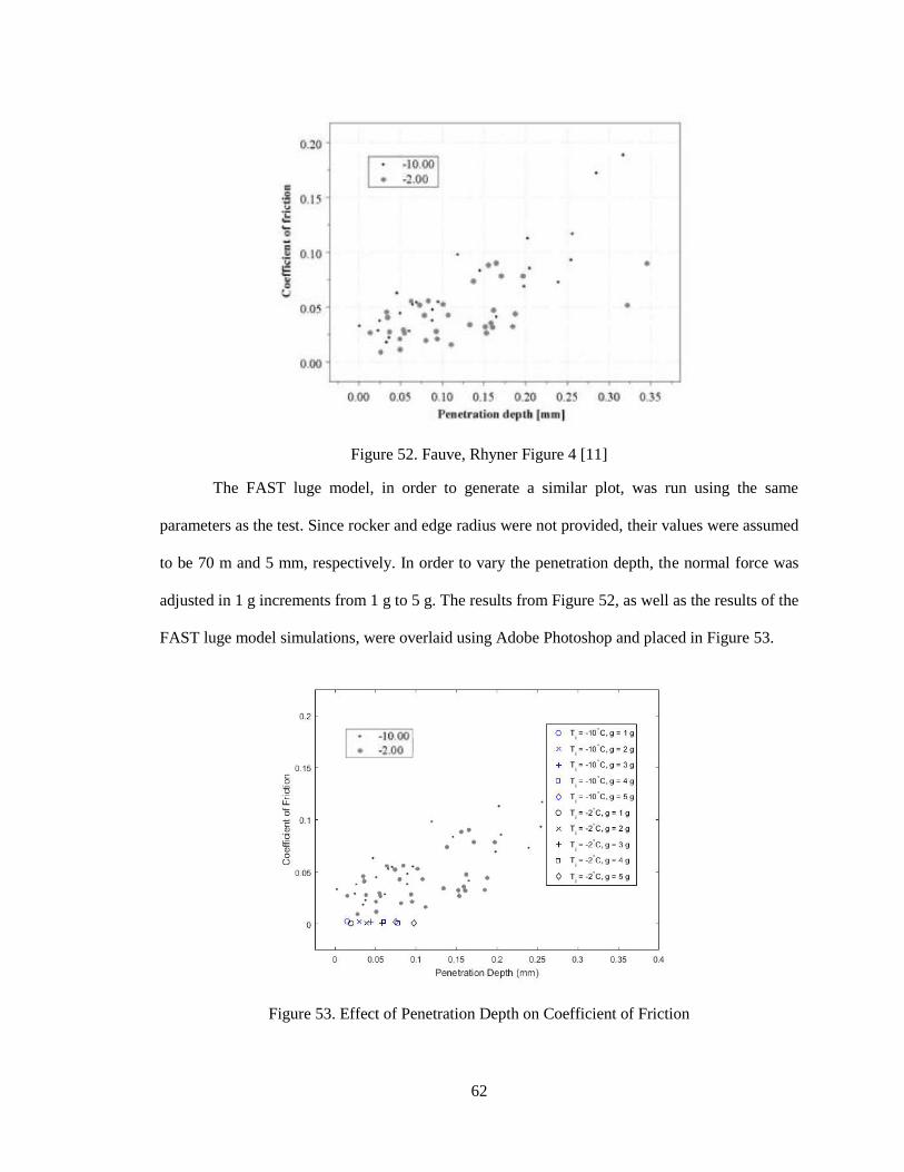
62

Figure 52. Fauve, Rhyner Figure 4 [11]

The FAST luge model, in order to generate a similar plot, was run using the same

parameters as the test. Since rocker and edge radius were not provided, their values were assumed

to be 70 m and 5 mm, respectively. In order to vary the penetration depth, the normal force was

adjusted in 1 g increments from 1 g to 5 g. The results from Figure 52, as well as the results of the

FAST luge model simulations, were overlaid using Adobe Photoshop and placed in Figure 53.

Figure 53. Effect of Penetration Depth on Coefficient of Friction

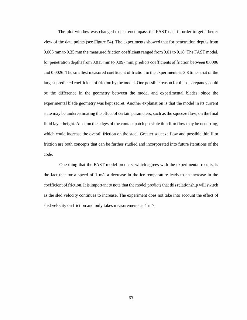
63

The plot window was changed to just encompass the FAST data in order to get a better

view of the data points (see Figure 54). The experiments showed that for penetration depths from

0.005 mm to 0.35 mm the measured friction coefficient ranged from 0.01 to 0.18. The FAST model,

for penetration depths from 0.015 mm to 0.097 mm, predicts coefficients of friction between 0.0006

and 0.0026. The smallest measured coefficient of friction in the experiments is 3.8 times that of the

largest predicted coefficient of friction by the model. One possible reason for this discrepancy could

be the difference in the geometry between the model and experimental blades, since the

experimental blade geometry was kept secret. Another explanation is that the model in its current

state may be underestimating the effect of certain parameters, such as the squeeze flow, on the final

fluid layer height. Also, on the edges of the contact patch possible thin film flow may be occurring,

which could increase the overall friction on the steel. Greater squeeze flow and possible thin film

friction are both concepts that can be further studied and incorporated into future iterations of the

code.

One thing that the FAST model predicts, which agrees with the experimental results, is

the fact that for a speed of 1 m/s a decrease in the ice temperature leads to an increase in the

coefficient of friction. It is important to note that the model predicts that this relationship will switch

as the sled velocity continues to increase. The experiment does not take into account the effect of

sled velocity on friction and only takes measurements at 1 m/s.

64

Figure 54. Effect of Penetration Depth on Coefficient of Friction Zoomed

Another portion of the experiment [11] included the comparison of the laboratory and field

conditions. The depth of the grooves left by luge sled blades was measured on flat sections of track

by taking imprints using Mikrosil two component silicon paste. The cuts left by the steels were

found to be between 0.06 and 0.08 mm when the ice temperature was -2 °C. The FAST model for

a flat section of track predicts the penetration depth of the runners to be closer to 0.02 mm.

Additional down forces due aerodynamics of the sled, as well as differences in the steel geometry

are possible partial reasons for the discrepancy.

65

CHAPTER 4: CONCLUSION

The luge ice-steel interaction model, converted from FAST 3.1b and FAST 3.2b, is meant

to be used as a Matlab function file. This function file will be incorporated into driver and track

dynamic models being developed. Inputs for this model include the force on the steel, temperature

of the ice surface, velocity of the sled, and geometry of the steel. Reaction of the steels on track

curves is taken into account by the increased normal loading and tracking the allowable lateral force

before side slip of the steel occurs.

The FAST luge model includes a set of assumptions and simplifications that may limit the

effectiveness under certain conditions. One of the limitations of the model are calculations made at

temperatures warmer than -1°C. Rapid deterioration of the ice surface hardness above this

temperature is not taken into account for the ice hardness calculations. During calculation of the

ploughing force, the area of the contact force of the steel was established to be equal to the force

on the runner divided by the hardness of the ice surface. The area of the contact patch, which

follows the curved surface of the runner edge profile, was assumed to be approximately equal to its

2-D projection onto the y-z plane. For this reason, although we are considering the difference

negligible, the model is slightly underestimating the magnitude of the contact force. The calculation

for the squeeze flow as well makes several assumptions, which are used to simplify the form of the

Navier-Stokes equation. These assumptions include constant applied pressure applied in both the

radial and longitudinal directions. This holds true for the sled moving down a straight section of

track, assuming that the hardness of the ice surface is constant. In the case of a banked turn, where

lateral forces are introduced, this does not necessarily hold true along the radial direction. The

model in its current state may be underestimating the effect of squeeze flow on increasing steel-ice

friction on curves. These are all areas that can be addressed in future iterations of the code, once

the function file is incorporated into the dynamic model and can be compared with track data.

In order to better understand the relationship between a luge steel and the ice surface, the

luge FAST model was run for a variety of input conditions. Adjustments to the temperature of the

66

ice surface revealed that, at lower sled velocities, temperatures closer to the melting temperature

correspond to increases in friction. At greater velocities, this trend shifts where warmer

temperatures lower the friction. The friction can be separated into ploughing force and Couette

flow shear components. The Couette flow shear makes up the greatest portion of the total friction,

and is most sensitive to temperature changes at lower sled speeds. The Couette flow follows the

trends for the overall friction, while for the ploughing force decreases in temperature correspond to

decreases in the ploughing force.

Changes in the edge radius of the steel revealed that a sharper edge radius translates to

lower coefficients of friction at low sled velocities and the opposite at high sled velocities. The

sensitivity of the friction to changes in edge radius is much greater at lower velocities. The Couette

flow shear for these runs was still the main source of the friction and decreases when the edge

radius is made smaller, regardless of sled velocity. For all sled velocities, the ploughing force

increases with decreases in edge radius. Analysis was completed as well to show how the edge

radius effects the lateral force limit on turns. A smaller edge radius was shown to increase the lateral

force limit almost 4 times its original value for a variety of ice temperatures when the edge radius

was changed from 0.014 m to 0.005 m. Even though at higher velocities a smaller edge radius leads

to increased friction, the percent difference is less than 1%. Once the FAST friction function file is

incorporated into the dynamic model, an analysis will need to be completed for a radius of 0.005

m to see if over the length of the run the benefits of the lower friction force at slower velocities and

higher allowable lateral force overcome the higher friction at later stages when the velocity is

greater. It is hypothesized that due to the much greater reduction in friction at lower velocities

compared to the increase at higher velocities and the larger lateral force limit allowing for tighter

turns down the track, a smaller edge radius will be desirable.

Allowing for variations in the steel rocker radius led to the observation that for a straight

and curved section of track a flatter rocker translates to lowered friction. Both the ploughing force

and the Couette flow shear decreased with increases in rocker radius. Even though the Couette flow

67

shear force makes up the majority of the friction force, the ploughing force was found to be more

sensitive than the Couette flow force to changes in R. One of the concerns with the flatter rocker

was that if the steel is flat enough, where the rocker radius is greater than the radius of the curve of

the track, two contact patches will be present instead of just one. Analysis showed that dual contact

patches actually decreased the overall friction. Although a flatter steel reduces friction, it reduces

amount of lateral force the sled can take before side slip occurs. The allowable lateral force for

various ice temperatures for a rocker of 10 m is approximately 1.6 times greater than the allowable

lateral force for a rocker of 70 m. Further analysis with the dynamic model will need to be

performed in order to see whether the decrease in allowable lateral force from increasing rocker

radius proves to have a greater or lesser effect on run time than the decrease in friction. Once this

is completed, the optimum rocker radius can be determined.

The effect of turns on the friction was approached in part by seeing how adjustments to the

down force affect the friction. Increases in loading were found to correspond to increases in both

the ploughing force and the Couette flow shear. The differences in normal forces caused the plots

of friction force to look quite different than the plot of coefficient of friction. The coefficient of

friction for various velocities drops at first, then continues to increase until the friction becomes

greater than those seen at 1 g. The most likely explanation for this is the rapid increase of a factor

like squeeze flow compared to the other values as the force on the steel gets larger. The model

predicts that at higher sled velocities and the largest loading condition of 5 g the friction is greatest,

which is consistent with existing literature that states that the greatest friction, not including the

start, is experienced on the last turn of the run. Although on the final turns of the track greater

downforce can be considered a disadvantage from a friction standpoint, the increase in the

allowable lateral force before side slip occurs may prove to be an even greater advantage since a

tighter turn is possible.

The FAST luge model was compared to results from experiments run in “Analysis and

Optimization of the Sliding Properties of Luge Steel Blades on Ice” [11]. Experimental results for

68

coefficient of friction were at a minimum 3.8 times larger than the model prediction at similar

penetration depths. Furthermore, penetration depths of the steel predicted by the model were

approximately a third of those measured on an actual Luge track. These discrepancies indicate that

further experimentation and study focusing on how the assumptions made in the model effect the

results is necessary. Areas of focus may include the squeeze flow calculation and possible thin film

flow on the contact area boundary.

The next step for this project will be to determine if the qualitative relationships covered

in this report remain consistent when making steps to improve the accuracy of the model. It is

important to note that the FAST Luge model in its current state is meant to be a stepping stone,

rather than a final product, and is to be used as a tool to continue to develop an increasingly accurate

Luge model as a whole. The purpose of this study was not to necessarily come to concrete

conclusions on the relationship between sled steel geometry and performance, but rather to act as

a baseline for future studies and analysis. An important part of this future analysis will be to conduct

a series of experiments to confirm the friction coefficient of the sled steels for the range of

environmental and geometric conditions covered. Eventual comparisons to real Luge track data

will be vital in order to fully understand the accuracy of this model and allow for proper tuning by

combining models of drag, ice friction, and sled dynamics. Once the overall model has the ability

to accurately predict run times, more parametric studies will need to be run to make decisions on

how to best improve track times.

By mathematically defining as many aspects of the sport of luge as possible, the hope is to

make the search for possible improvements quicker and more efficient. It is unreasonable to expect

a mathematical model to fully replace human experience and intuition in race and sled design

decisions. The goal is that this tool one day will have the ability to be used as a catalyst to help

consistently propel team USA to the top of the podium in the sport of Luge.

69

BIBLIOGRAPHY

[1] Bradley, Pat. “USA Luge Keeps Headquarters In Lake Placid.” WAMC, 24 May 2016,

wamc.org/post/usa-luge-keeps-headquarters-lake-placid.

[2] “The Luge Start.” Team USA, www.teamusa.org/-/media/USA_Luge/Documents/5start

.pdf?la=en&hash.

[3] “Winter Olympics 2014 Preview: Luge Training | Sochi Olympics.” YouTube, Wall Street

Journal, 18 Oct. 2013, www.youtube.com/watch?v=qovhV-uBVqo.

[4] “About FIL.” International Luge Federation, http://www.fil-luge.org/en/about-fil.

[5] “How Luge Works.” howstuffworks, https://adventure.howstuffworks.com/outdoor-

activities/snow-sports/luge2.htm.

[6] IRO International Luge Regulations Artificial Track 2016 Edition. International Luge

Federation, www.fil-luge.org/en/rules/rules-artificial-track.

[7] Braghin, Francesco, Mauro Donzelli, Stefano Melzi, and Edoardo Sabbioni. "A Driver Model

of a Two-man Bobsleigh." Sports Engineering 13.4 (2011): 181-93. Engineering Village.

Web. 4 Apr. 2017.

[8] Mössner, Martin, Michael Hasler, Kurt Schindelwig, Peter Kaps, and Werner Nachbauer. "An

Approximate Simulation Model for Initial Luge Track Design." Journal of

Biomechanics 44.5 (2011): 892-96. Engineering Village. Web. 4 Apr. 2017.

[9] Poirier, Louis. Ice Friction in the Sport of Bobsleigh. Thesis. University of Calgary, 2011.

N.p.: n.p., n.d. ResearchGate. Web. 10 Apr. 2017.

[10] A. Penny, E. Lozowski, T. Forest, C. Fong, S. Maw, P. Montgomery, and N. Sinha,

“Speedskate ice friction: review and numerical model FAST 1.0,” in Physics and Chemistry

of Ice, W. F. Kuhs, Ed. Roy. Soc. Chem., 2007, pp. 495–504.

[11] Fauve M., Rhyner H. (2008) “Analysis and Optimization of the Sliding Properties of Luge

Steel Blades on Ice (P111).” In: The Engineering of Sport 7. Springer, Paris.

70

[12] Balakin, V. A. "Friction Performance of Sports Luges and Bobsleds Sliding along Ice

Track."Journal of Friction and Wear 17.1 (1996): 29. Engineering Village. Web. 10 Apr.

2017.

[13] Bluhm, Hendrik, Takahito Inoue, and Miquel Salmeron. "Friction of Ice Measured Using

Lateral Force Microscopy." Physical Review B 61.11 (2000): 7760-765. Web. 12 Apr. 2017.

[14] Braghin, Francesco, Federico Cheli, Stefano Melzi, and Edoardo Sabbioni. "Experimental

Assessment of Bobsleigh Dynamics and Ice-Skate Contact Forces." Topics in Modal

Analysis II, Volume 6 Conference Proceedings of the Society for Experimental Mechanics

Series (2012): 487-98. Engineering Village. Web. 6 Apr. 2017.

[15] Colbeck, S. C. "Pressure Melting and Ice Skating." American Journal of Physics 63.10

(1995): 888-90. Web. 6 Apr. 2017.

[16] Federolf, Peter, and Benno Nigg. "Skating Performance in Ice Hockey When Using a Flared

Skate Blade Design." Cold Regions Science and Technology 70 (2012): 12-18. Web. 6 Apr.

2017.

[17] Fowler, A.J., and A. Bejan. "Contact Melting during Sliding on Ice." International Journal of

Heat and Mass Transfer 36.5 (1993): 1171-179. Engineering Village. Web. 6 Apr. 2017.

[18] “Highlights of Sledding and FIL History.” International Luge Federation, www.fil-

luge.org/en/about-fil/history.

[19] “History.” Team USA, https://www.teamusa.org/usa-luge/history-and-fast-facts.

[20] Incropera, Frank P., and David P. DeWitt. Introduction to Heat Transfer. 6th ed., Wiley,

2011.

[21] "IRO International Luge Regulations." (2016): n. pag. Web. <http://www.fil-

luge.org/cdn/uploads/iro-2016-nb-english-final.pdf>.

[22] Kietzig, Anne-Marie, Savvas G. Hatzikiriakos, and Peter Englezos. "Physics of Ice Friction."

Journal of Applied Physics 107.8 (2010): 081101. Engineering Village. Web. 6 Apr. 2017.

71

[23] Koning, Jos J. De, Gert De Groot, and Gerrit Jan Van Ingen Schenau. "Ice Friction during

Speed Skating." Journal of Biomechanics 25.6 (1992): 565-71. Engineering Village. Web. 6

Apr. 2017.

[24] Lozowski, Edward, Krzysztof Szilder, Sean Maw, and Alexis Morris. "A Model of Ice

Friction for Skeleton Sled Runners." Proceedings of the 24th International Ocean and Polar

Engineering Conference. N.p., n.d. Web. 10 Apr. 2017.

[25] Makkonen, Lasse, and Maria Tikanmaki. “Modeling the Friction of Ice.” Compendex,

Engineering Village, June 2014.

[26] Munson, Bruce Roy, et al. Fundamentals of Fluid Mechanics. 7th ed., John Wiley & Sons,

Inc., 2013.

[27] Sato, Kazuo, Teruyoshi Sadahiro, Masami Iwase, Hiroo Shinbara, and Shoshiro

Hatakeyama. "Modeling and Analysis for Ice Skating Blade." ICROS-SICE International

Joint Conference 2009. N.p., n.d. Web. 6 Apr. 2017.

[28] Steinbeiser, Andrew. “Cutting-Edge Technology You Can Spot at the Sochi

Olympics.”Discover, 13 Feb. 2014, blogs.discovermagazine.com/crux/2014/02/13/ cutting-

edge-technology-you-can-spot-at-the-sochi-olympics/#.Wf-FtFtSyUm.

[29] “The History of the Sport of Luge.” Team USA, https://www.teamusa.org/-

/media/USA_Luge/Documents/10historybroch.pdf?la.

72

APPENDIX: MATLAB CODE

A.1 FAST Bobsled Model Master File (Poirier Comparison)

%% RUN FAST (Bobsled Model)

% Written by: Brandon Stell

% Based off of FAST 3.1b/3.2b written by Louis Poirier:

% Poirier, Louis. Ice Friction in the Sport of Bobsleigh. Thesis. University

% of Calgary, 2011. N.p.: n.p., n.d. ResearchGate. Web. 10 Apr. 2017.

% Date Last Updated: 10/10/17

mm = [1 0];

T_im = [-2 -6 -10 -14];

vm = [1 5 10 15 20 25 30 35 40];

U_runners = zeros(length(vm),length(T_im),length(mm));

k = 1;

for m = mm

j = 1;

for T_i = T_im

i = 1;

for v = vm

U_runners(i,j,k) = FAST(v,T_i,m,0);

i = i+1;

end

j = j+1;

end

k = k+1;

end

U_pp = [0.88095 1.88095 2.73810 3.50000;...

1.09524 1.40476 1.76190 2.05952;...

1.25000 1.38095 1.55952 1.73810;...

1.35714 1.42857 1.52381 1.64286;...

1.45238 1.47619 1.53571 1.61905;...

1.54762 1.54762 1.55952 1.60714;...

1.61905 1.59524 1.59524 1.61905;...

1.69048 1.64286 1.64286 1.64286;...

1.76190 1.71429 1.69048 1.66667]; % parallel tracks

U_ps = [0.88095 1.89286 2.84524 3.52381;...

1.04762 1.33333 1.66667 2.00000;...

1.19048 1.32143 1.50000 1.66667;...

1.28571 1.35714 1.47619 1.57143;...

1.33333 1.41667 1.48810 1.53571;...

1.38095 1.47619 1.50000 1.53571;...

1.42857 1.53571 1.54762 1.55952;...

1.47619 1.59524 1.58333 1.58333;...

1.50000 1.64286 1.61905 1.59524;]; % same track

73

figure(1)

plot(vm',U_pp(:,1),'b-',vm',U_runners(:,1,1),'b--',vm',U_pp(:,2),'g-',vm',U_runners(:,2,1),'g--

',vm',U_pp(:,3),'r-',vm',U_runners(:,3,1),'r--',vm',U_pp(:,4),'k-',vm',U_runners(:,4,1),'k--')

xlabel 'Sled Speed (m/s)'

ylabel 'Coefficient of friction (10^-3)'

title 'Parallel Tracks'

legend '-2^{\circ} (Poirier)' '-2^{\circ} (Stell)' '-6^{\circ} (Poirier)' '-6^{\circ} (Stell)' '-10^{\circ}

(Poirier)' '-10^{\circ} (Stell)' '-14^{\circ} (Poirier)' '-14^{\circ} (Stell)'

axis([0 45 0 4])

PerDiff_P = abs(U_runners(:,:,1)-U_pp)./((U_runners(:,:,1)+U_pp)/2)*100;

figure(2)

subplot(2,2,1)

plot(vm',PerDiff_P(:,1),'k-')

xlabel 'Sled Speed (m/s)'

ylabel 'COF Percent Difference (%)'

title 'Parallel Tracks (T = -2^{\circ})'

axis([0 40 0 35])

subplot(2,2,2)

plot(vm',PerDiff_P(:,2),'k-')

xlabel 'Sled Speed (m/s)'

ylabel 'COF Percent Difference (%)'

title 'Parallel Tracks (T = -6^{\circ})'

axis([0 40 0 35])

subplot(2,2,3)

plot(vm',PerDiff_P(:,3),'k-')

xlabel 'Sled Speed (m/s)'

ylabel 'COF Percent Difference (%)'

title 'Parallel Tracks (T = -10^{\circ})'

axis([0 40 0 35])

subplot(2,2,4)

plot(vm',PerDiff_P(:,4),'k-')

xlabel 'Sled Speed (m/s)'

ylabel 'COF Percent Difference (%)'

title 'Parallel Tracks (T = -14^{\circ})'

axis([0 40 0 35])

figure(3)

plot(vm',U_ps(:,1),'b-',vm',U_runners(:,1,2),'b--',vm',U_ps(:,2),'g-',vm',U_runners(:,2,2),'g--

',vm',U_ps(:,3),'r-',vm',U_runners(:,3,2),'r--',vm',U_ps(:,4),'k-',vm',U_runners(:,4,2),'k--')

xlabel 'Sled Speed (m/s)'

ylabel 'Coefficient of friction (10^-3)'

title 'Overlapping Tracks'

legend '-2^{\circ} (Poirier)' '-2^{\circ} (Stell)' '-6^{\circ} (Poirier)' '-6^{\circ} (Stell)' '-10^{\circ}

(Poirier)' '-10^{\circ} (Stell)' '-14^{\circ} (Poirier)' '-14^{\circ} (Stell)'

axis([0 45 0 4])

PerDiff_S = abs(U_runners(:,:,2)-U_ps)./((U_runners(:,:,2)+U_ps)/2)*100;

74

figure(4)

subplot(2,2,1)

plot(vm',PerDiff_S(:,1),'k-')

xlabel 'Sled Speed (m/s)'

ylabel 'COF Percent Difference (%)'

title 'Overlapping Tracks (T = -2^{\circ})'

axis([0 40 0 35])

subplot(2,2,2)

plot(vm',PerDiff_S(:,2),'k-')

xlabel 'Sled Speed (m/s)'

ylabel 'COF Percent Difference (%)'

title 'Overlapping Tracks (T = -6^{\circ})'

axis([0 40 0 35])

subplot(2,2,3)

plot(vm',PerDiff_S(:,3),'k-')

xlabel 'Sled Speed (m/s)'

ylabel 'COF Percent Difference (%)'

title 'Overlapping Tracks (T = -10^{\circ})'

axis([0 40 0 35])

subplot(2,2,4)

plot(vm',PerDiff_S(:,4),'k-')

xlabel 'Sled Speed (m/s)'

ylabel 'COF Percent Difference (%)'

title 'Overlapping Tracks (T = -14^{\circ})'

axis([0 40 0 35])

A.2. FAST Bobsled Model Function File (Poirier Comparison)

%% FAST FUNCTION FILE (Bobsled Model)

% Written by: Brandon Stell

% Based off of FAST 3.1b/3.2b written by Louis Poirier:

% Poirier, Louis. Ice Friction in the Sport of Bobsleigh. Thesis. University

% of Calgary, 2011. N.p.: n.p., n.d. ResearchGate. Web. 10 Apr. 2017.

% Date Last Updated: 10/10/17

function [U_runners, size] = FAST(v,T_i,m,p)

tic

%% Input Variables

R = 34; % m, rocker value (20-48 m)

r_c = 4.75/1000 % m, cross-sectional radii, 2 man (4-5.5 mm)

F_fg = 0.44*390*9.81/2; % N, sled weight distributed to one of the front runners (44% total sled

weight of 390 kg)

F_rg = 0.56*390*9.81/2; % N, sled weight distributed to one of the front runners (56% total sled

weight of 390 kg)

u_w = 1.79*10^-3; % kg/m/s, dynamic viscosity of water

k_i = 2.25; % W/m/K, thermal conductivity of ice for T_i = -5 deg Celsius (temperature

dependence negligable)

c_i = 2.04*10^3; % J/kg/K, specific heat of ice for T_i = -9 deg Celsius (temperature dependence

negligable)

75

p_i = 917.5; % kg/m^3, density of ice for T_i = -4 deg Celsius (temperature dependence

negligable)

p_w = 1000; % kg/m^3, density of water

l_f = 3.34*10^5; % J/kg, latent heat of fusion of ice

h_ice = 0.025; % m, thickness of the ice

dz = 10^-5;%10^-6 (recommended); % m, step size along runner length

dy = 10^-6;%10^-7 (recommended); % m, step size along width of runner

p_s = 7650; % kg/m^3, density of 17-4 steel

c_s = 460; % J/kg/C, specific heat of 17-4 steel

k_s = 14; % W/m/C, thermal conductivity of 17-4 steel

%% Solution

% Runner Ice Contact Calculations Front Runners

T_b = T_i-2; % deg. Celsius, temperature of the ice base, set to two degrees less than the surface

temperature by recommendation, parameter could benefit from further study

P = (-0.6*T_i+14.7)*10^6; % Pa, ice hardness ((-0.6+/-0.4)T+(14.7+/-2.1)) MPa

d_max = F_fg/(pi*P*sqrt(R*r_c)); % m, maximum penetration of front runners

l_s = sqrt(2*R*d_max-d_max^2); % m, maximum contact length front runners

y_max = sqrt(2*r_c*d_max-d_max^2); % m, half-width front runners

A_f = pi*y_max*l_s/2; % m^2, front runner contact area in the plane of the ice surface

% Runner Ice Contact Calculations Rear Runners

if m == 1 % front and rear runners are slightly out of alignment

d_maxr = F_rg/(pi*P*sqrt(R*r_c)); % m, maximum penetration of rear runners

l_sr = sqrt(2*R*d_maxr-(d_maxr)^2); % m, maximum contact length of rear runners

y_maxr = sqrt(2*r_c*d_maxr-(d_maxr)^2); % m, half-width of rear runners

elseif m == 0 % front and rear runners are perfectly aligned

d_maxr = 2*d_max;

test = (y_max+sqrt(2*r_c*d_maxr-d_maxr^2))*sqrt(2*R*(d_maxr-d_max)-(d_maxr-

d_max)^2);

check = abs(test-F_rg/P)/test;

while check > 0.001 || check < 0

if check > 0.001

d_maxr = d_maxr - 10^-7.5;

test = (y_max+sqrt(2*r_c*d_maxr-d_maxr^2))*sqrt(2*R*(d_maxr-d_max)-(d_maxr-

d_max)^2);

check = abs(test-F_rg/P)/test;

elseif check < 0

d_maxr = d_maxr + 10^-7.5;

test = (y_max+sqrt(2*r_c*d_maxr-d_maxr^2))*sqrt(2*R*(d_maxr-d_max)-(d_maxr-

d_max)^2);

check = abs(test-F_rg/P)/test;

else

end

end

l_sr = sqrt(2*R*(d_maxr-d_max)-(d_maxr-d_max)^2);

y_maxr = sqrt(2*r_c*d_maxr-d_maxr^2);

else

disp('Error: invalid model selection')

end

A_r = (y_max+y_maxr)*l_sr; % m^2, rear runner contact area in the plane of the ice surface

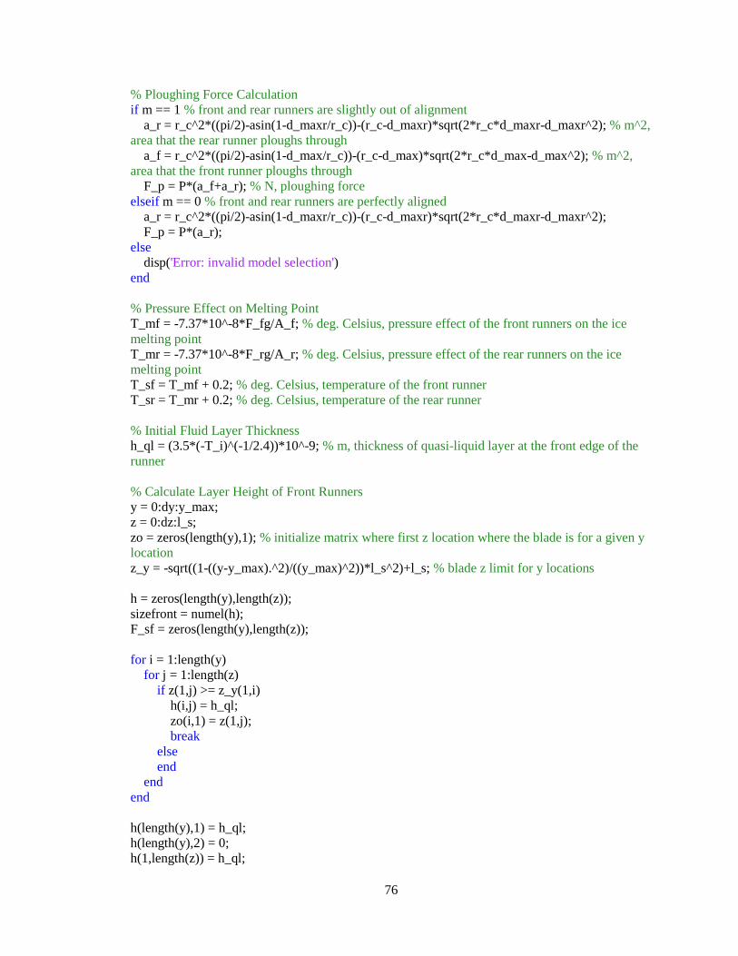
76

% Ploughing Force Calculation

if m == 1 % front and rear runners are slightly out of alignment

a_r = r_c^2*((pi/2)-asin(1-d_maxr/r_c))-(r_c-d_maxr)*sqrt(2*r_c*d_maxr-d_maxr^2); % m^2,

area that the rear runner ploughs through

a_f = r_c^2*((pi/2)-asin(1-d_max/r_c))-(r_c-d_max)*sqrt(2*r_c*d_max-d_max^2); % m^2,

area that the front runner ploughs through

F_p = P*(a_f+a_r); % N, ploughing force

elseif m == 0 % front and rear runners are perfectly aligned

a_r = r_c^2*((pi/2)-asin(1-d_maxr/r_c))-(r_c-d_maxr)*sqrt(2*r_c*d_maxr-d_maxr^2);

F_p = P*(a_r);

else

disp('Error: invalid model selection')

end

% Pressure Effect on Melting Point

T_mf = -7.37*10^-8*F_fg/A_f; % deg. Celsius, pressure effect of the front runners on the ice

melting point

T_mr = -7.37*10^-8*F_rg/A_r; % deg. Celsius, pressure effect of the rear runners on the ice

melting point

T_sf = T_mf + 0.2; % deg. Celsius, temperature of the front runner

T_sr = T_mr + 0.2; % deg. Celsius, temperature of the rear runner

% Initial Fluid Layer Thickness

h_ql = (3.5*(-T_i)^(-1/2.4))*10^-9; % m, thickness of quasi-liquid layer at the front edge of the

runner

% Calculate Layer Height of Front Runners

y = 0:dy:y_max;

z = 0:dz:l_s;

zo = zeros(length(y),1); % initialize matrix where first z location where the blade is for a given y

location

z_y = -sqrt((1-((y-y_max).^2)/((y_max)^2))*l_s^2)+l_s; % blade z limit for y locations

h = zeros(length(y),length(z));

sizefront = numel(h);

F_sf = zeros(length(y),length(z));

for i = 1:length(y)

for j = 1:length(z)

if z(1,j) >= z_y(1,i)

h(i,j) = h_ql;

zo(i,1) = z(1,j);

break

else

end

end

end

h(length(y),1) = h_ql;

h(length(y),2) = 0;

h(1,length(z)) = h_ql;

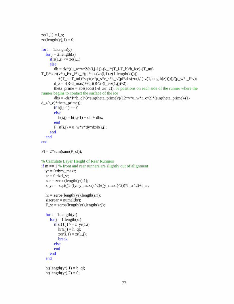
77

zo(1,1) = l_s;

zo(length(y),1) = 0;

for i = 1:length(y)

for j = 2:length(z)

if z(1,j) <= zo(i,1)

else

dh = dz*((u_w*v^2/h(i,j-1))-(k_i*(T_i-T_b)/h_ice)-(T_mf-

T_i)*sqrt(v*p_i*c_i*k_i/(pi*abs(zo(i,1)-z(1,length(z)))))...

+(T_sf-T_mf)*sqrt(v*p_s*c_s*k_s/(pi*abs(zo(i,1)-z(1,length(z))))))/(p_w*l_f*v);

d_z = -(R-d_max)+sqrt(R^2-(l_s-z(1,j))^2);

theta_prime = abs(acos(1-d_z/r_c)); % positions on each side of the runner where the

runner begins to contact the surface of the ice

dhs = -dz*P*h_ql^3*sin(theta_prime)/((12*v*u_w*r_c^2)*(sin(theta_prime)-(1-

d_z/r_c)*theta_prime));

if h(i,j-1) == 0

else

h(i,j) = h(i,j-1) + dh + dhs;

end

F_sf(i,j) = u_w*v*dy*dz/h(i,j);

end

end

end

Ff = 2*sum(sum(F_sf));

% Calculate Layer Height of Rear Runners

if m == 1 % front and rear runners are slightly out of alignment

yr = 0:dy:y_maxr;

zr = 0:dz:l_sr;

zor = zeros(length(yr),1);

z_yr = -sqrt((1-((yr-y_maxr).^2)/((y_maxr)^2))*l_sr^2)+l_sr;

hr = zeros(length(yr),length(zr));

sizerear = numel(hr);

F_sr = zeros(length(yr),length(zr));

for i = 1:length(yr)

for j = 1:length(zr)

if zr(1,j) >= z_yr(1,i)

hr(i,j) = h_ql;

zor(i,1) = zr(1,j);

break

else

end

end

end

hr(length(yr),1) = h_ql;

hr(length(yr),2) = 0;

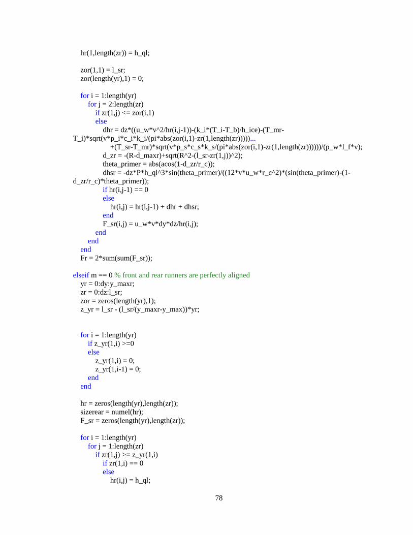
78

hr(1,length(zr)) = h_ql;

zor(1,1) = l_sr;

zor(length(yr),1) = 0;

for i = 1:length(yr)

for j = 2:length(zr)

if zr(1,j) <= zor(i,1)

else

dhr = dz*((u_w*v^2/hr(i,j-1))-(k_i*(T_i-T_b)/h_ice)-(T_mr-

T_i)*sqrt(v*p_i*c_i*k_i/(pi*abs(zor(i,1)-zr(1,length(zr)))))...

+(T_sr-T_mr)*sqrt(v*p_s*c_s*k_s/(pi*abs(zor(i,1)-zr(1,length(zr))))))/(p_w*l_f*v);

d_zr = -(R-d_maxr)+sqrt(R^2-(l_sr-zr(1,j))^2);

theta_primer = abs(acos(1-d_zr/r_c));

dhsr = -dz*P*h_ql^3*sin(theta_primer)/((12*v*u_w*r_c^2)*(sin(theta_primer)-(1-

d_zr/r_c)*theta_primer));

if hr(i,j-1) == 0

else

hr(i,j) = hr(i,j-1) + dhr + dhsr;

end

F_sr(i,j) = u_w*v*dy*dz/hr(i,j);

end

end

end

Fr = 2*sum(sum(F_sr));

elseif m == 0 % front and rear runners are perfectly aligned

yr = 0:dy:y_maxr;

zr = 0:dz:l_sr;

zor = zeros(length(yr),1);

z_yr = l_sr - (l_sr/(y_maxr-y_max))*yr;

for i = 1:length(yr)

if z_yr(1,i) >=0

else

z_yr(1,i) = 0;

z_yr(1,i-1) = 0;

end

end

hr = zeros(length(yr),length(zr));

sizerear = numel(hr);

F_sr = zeros(length(yr),length(zr));

for i = 1:length(yr)

for j = 1:length(zr)

if zr(1,j) >= z_yr(1,i)

if zr(1,i) == 0

else

hr(i,j) = h_ql;

79

end

zor(i,1) = zr(1,j);

break

else

end

end

end

hr((length(yr)-length(y)+1):length(yr),1) = h(:,length(z));

hr(length(yr),2) = 0;

hr(1,length(zr)) = h_ql;

zor(1,1) = l_sr;

for i = 1:length(yr)

for j = 2:length(zr)

if zr(1,j) <= zor(i,1)

else

dhr = dz*((u_w*v^2/hr(i,j-1))-(k_i*(T_i-T_b)/h_ice)-(T_mr-

T_i)*sqrt(v*p_i*c_i*k_i/(pi*abs(zor(i,1)-zr(1,length(zr)))))...

+(T_sr-T_mr)*sqrt(v*p_s*c_s*k_s/(pi*abs(zor(i,1)-zr(1,length(zr))))))/(p_w*l_f*v);

d_zr = -(R-d_maxr)+sqrt(R^2-(l_sr-zr(1,j))^2);

theta_primer = abs(acos(1-d_zr/r_c));

dhsr = -dz*P*h_ql^3*sin(theta_primer)/((12*v*u_w*r_c^2)*(sin(theta_primer)-(1-

d_zr/r_c)*theta_primer));

hr(i,j) = hr(i,j-1) + dhr + dhsr;

F_sr(i,j) = u_w*v*dy*dz/hr(i,j);

end

end

end

Fr = 2*sum(sum(F_sr));

else

disp('Error: invalid model selection')

end

F = Fr+Ff+F_p;

U_runners = F/(F_fg+F_rg)*10^3; % friction runners

if p == 1

hsurf = h;

for i = 1:length(y)

for j = 1:length(z)

if hsurf(i,j) == 0

hsurf(i,j) = NaN;

else

end

end

end

hsurf_max = max(max(hsurf));

hsurf_min = min(min(hsurf));

80

hsurfr = hr;

for i = 1:length(yr)

for j = 1:length(zr)

if hsurfr(i,j) == 0

hsurfr(i,j) = NaN;

else

end

end

end

hsurfr_max = max(max(hsurfr));

hsurfr_min = min(min(hsurfr));

figure(1)

dhsurf = hsurf_max/50;

t = 0:dhsurf:hsurf_max;

colormap(jet)

contourf(z, y-y_max, hsurf, t, 'LineStyle', 'none')

colorbar

caxis ([hsurf_min, hsurf_max])

axis square tight

title('Front Runner Liquid Layer Thickness (m)')

xlabel('z (m)')

ylabel('y (m)')

figure(2)

dhsurfr = hsurfr_max/50;

vr = 0:dhsurfr:hsurfr_max;

colormap(jet)

contourf(zr, yr-y_maxr, hsurfr, vr, 'LineStyle', 'none')

colorbar

caxis ([hsurfr_min, hsurfr_max])

axis square tight

title('Rear Runner Liquid Layer Thickness (m)')

xlabel('z (m)')

ylabel('y (m)')

else

toc

end

size = sizefront+sizerear;

toc

A.3. Convergence Study

%% Convergence Study

% Written by: Brandon Stell

% Date Last Updated: 10/31/17

elem = [2340 55856 222253 1385764 2463549 3542170 5538403 6833129];

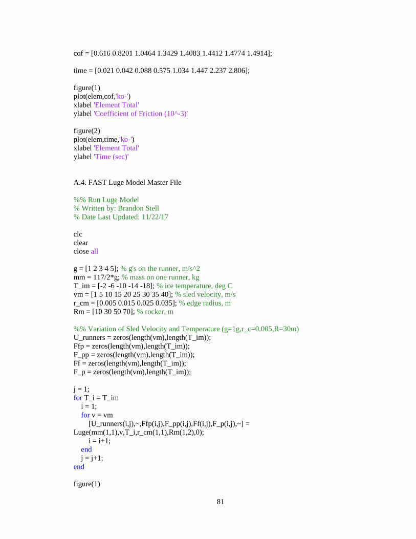
81

cof = [0.616 0.8201 1.0464 1.3429 1.4083 1.4412 1.4774 1.4914];

time = [0.021 0.042 0.088 0.575 1.034 1.447 2.237 2.806];

figure(1)

plot(elem,cof,'ko-')

xlabel 'Element Total'

ylabel 'Coefficient of Friction (10^-3)'

figure(2)

plot(elem,time,'ko-')

xlabel 'Element Total'

ylabel 'Time (sec)'

A.4. FAST Luge Model Master File

%% Run Luge Model

% Written by: Brandon Stell

% Date Last Updated: 11/22/17

clc

clear

close all

g = [1 2 3 4 5]; % g's on the runner, m/s^2

mm = 117/2*g; % mass on one runner, kg

T_im = [-2 -6 -10 -14 -18]; % ice temperature, deg C

vm = [1 5 10 15 20 25 30 35 40]; % sled velocity, m/s

r_cm = [0.005 0.015 0.025 0.035]; % edge radius, m

Rm = [10 30 50 70]; % rocker, m

%% Variation of Sled Velocity and Temperature (g=1g,r_c=0.005,R=30m)

U_runners = zeros(length(vm),length(T_im));

Ffp = zeros(length(vm),length(T_im));

F_pp = zeros(length(vm),length(T_im));

Ff = zeros(length(vm),length(T_im));

F_p = zeros(length(vm),length(T_im));

j = 1;

for T_i = T_im

i = 1;

for v = vm

[U_runners(i,j),~,Ffp(i,j),F_pp(i,j),Ff(i,j),F_p(i,j),~] =

Luge(mm(1,1),v,T_i,r_cm(1,1),Rm(1,2),0);

i = i+1;

end

j = j+1;

end

figure(1)

82

plot(vm',U_runners(:,1),'b-',vm',U_runners(:,2),'g-',vm',U_runners(:,3),'r-',vm',U_runners(:,4),'k-

',vm',U_runners(:,5),'c-')

xlabel 'Sled Speed (m/s)'

ylabel 'Coefficient of Friction (10^-3)'

legend 'T_i = -2^{\circ}C' 'T_i = -6^{\circ}C' 'T_i = -10^{\circ}C' 'T_i = -14^{\circ}C' 'T_i = -

18^{\circ}C'

axis([0 45 0.75 5])

grid ON

figure(2)

plot(vm',Ffp(:,1),'b-',vm',Ffp(:,2),'g-',vm',Ffp(:,3),'r-',vm',Ffp(:,4),'k-',vm',Ffp(:,5),'c-')

title '(A) Couette Flow'

xlabel 'Sled Speed (m/s)'

ylabel 'Percentage of Friction (%)'

legend 'T_i = -2^{\circ}C' 'T_i = -6^{\circ}C' 'T_i = -10^{\circ}C' 'T_i = -14^{\circ}C' 'T_i = -

18^{\circ}C'

axis([0 45 0 100])

grid ON

figure(3)

plot(vm',F_pp(:,1),'b-',vm',F_pp(:,2),'g-',vm',F_pp(:,3),'r-',vm',F_pp(:,4),'k-',vm',F_pp(:,5),'c-')

title '(B) Ploughing Force'

xlabel 'Sled Speed (m/s)'

ylabel 'Percentage of Friction (%)'

legend 'T_i = -2^{\circ}C' 'T_i = -6^{\circ}C' 'T_i = -10^{\circ}C' 'T_i = -14^{\circ}C' 'T_i = -

18^{\circ}C'

axis([0 45 0 100])

grid ON

figure(4)

plot(vm',Ff(:,1),'b-',vm',Ff(:,2),'g-',vm',Ff(:,3),'r-',vm',Ff(:,4),'k-',vm',Ff(:,5),'c-')

title '(A) Couette Flow'

xlabel 'Sled Speed (m/s)'

ylabel 'Friction Force (N)'

legend 'T_i = -2^{\circ}C' 'T_i = -6^{\circ}C' 'T_i = -10^{\circ}C' 'T_i = -14^{\circ}C' 'T_i = -

18^{\circ}C'

axis([0 45 0 2.5])

grid ON

figure(5)

plot(vm',F_p(:,1),'b-',vm',F_p(:,2),'g-',vm',F_p(:,3),'r-',vm',F_p(:,4),'k-',vm',F_p(:,5),'c-')

title '(B) Ploughing Force'

xlabel 'Sled Speed (m/s)'

ylabel 'Friction Force (N)'

legend 'T_i = -2^{\circ}C' 'T_i = -6^{\circ}C' 'T_i = -10^{\circ}C' 'T_i = -14^{\circ}C' 'T_i = -

18^{\circ}C'

axis([0 45 0 2.5])

grid ON

PerDiff1 = zeros(length(vm),length(T_im));

for i = 1:length(T_im)-1

PerDiff1(:,i) = (U_runners(:,i+1)-U_runners(:,1))./((U_runners(:,1)+U_runners(:,i+1))/2)*100;

end

83

figure(6)

plot(vm',zeros(length(vm),1),'b-',vm',PerDiff1(:,1),'g-',vm',PerDiff1(:,2),'r-',vm',PerDiff1(:,3),'k-

',vm',PerDiff1(:,4),'c-')

xlabel 'Sled Speed (m/s)'

ylabel 'COF Percent Difference (%)'

legend 'T_i = -2^{\circ}C' 'T_i = -6^{\circ}C' 'T_i = -10^{\circ}C' 'T_i = -14^{\circ}C' 'T_i = -

18^{\circ}C'

grid ON

%% Variation of Sled Velocity and Edge Radius (g=1g,T_i=-10degC,R=30m)

U_runners2 = zeros(length(vm),length(r_cm));

Ffp2 = zeros(length(vm),length(T_im));

F_pp2 = zeros(length(vm),length(T_im));

Ff2 = zeros(length(vm),length(T_im));

F_p2 = zeros(length(vm),length(T_im));

j = 1;

for r_c = r_cm

i = 1;

for v = vm

[U_runners2(i,j),~,Ffp2(i,j),F_pp2(i,j),Ff2(i,j),F_p2(i,j),~] =

Luge(mm(1,1),v,T_im(1,3),r_c,Rm(1,2),0);

i = i+1;

end

j = j+1;

end

figure(7)

plot(vm',U_runners2(:,1),'b-',vm',U_runners2(:,2),'g-',vm',U_runners2(:,3),'r-

',vm',U_runners2(:,4),'k-')

xlabel 'Sled Speed (m/s)'

ylabel 'Coefficient of Friction (10^-3)'

legend 'r_c = 0.005 m' 'r_c = 0.008 m' 'r_c = 0.011 m' 'r_c = 0.014 m'

axis([0 45 1.5 3.5])

figure(8)

plot(vm',Ffp2(:,1),'b-',vm',Ffp2(:,2),'g-',vm',Ffp2(:,3),'r-',vm',Ffp2(:,4),'k-')

title '(A) Couette Flow'

xlabel 'Sled Speed (m/s)'

ylabel 'Percentage of Friction (%)'

legend 'r_c = 0.005 m' 'r_c = 0.008 m' 'r_c = 0.011 m' 'r_c = 0.014 m'

axis([0 45 0 100])

figure(9)

plot(vm',F_pp2(:,1),'b-',vm',F_pp2(:,2),'g-',vm',F_pp2(:,3),'r-',vm',F_pp2(:,4),'k-')

title '(B) Ploughing Force'

xlabel 'Sled Speed (m/s)'

ylabel 'Percentage of Friction (%)'

legend 'r_c = 0.005 m' 'r_c = 0.008 m' 'r_c = 0.011 m' 'r_c = 0.014 m'

axis([0 45 0 100])

84

figure(10)

plot(vm',Ff2(:,1),'b-',vm',Ff2(:,2),'g-',vm',Ff2(:,3),'r-',vm',Ff2(:,4),'k-')

title '(A) Couette Flow'

xlabel 'Sled Speed (m/s)'

ylabel 'Friction Force (N)'

legend 'r_c = 0.005 m' 'r_c = 0.008 m' 'r_c = 0.011 m' 'r_c = 0.014 m'

axis([0 45 0 2])

figure(11)

plot(vm',F_p2(:,1),'b-',vm',F_p2(:,2),'g-',vm',F_p2(:,3),'r-',vm',F_p2(:,4),'k-')

title '(B) Ploughing Force'

xlabel 'Sled Speed (m/s)'

ylabel 'Friction Force (N)'

legend 'r_c = 0.005 m' 'r_c = 0.008 m' 'r_c = 0.011 m' 'r_c = 0.014 m'

axis([0 45 0 2])

PerDiff2 = zeros(length(vm),length(r_cm));

for i = 1:length(r_cm)-1

PerDiff2(:,i) = (U_runners2(:,i+1)-

U_runners2(:,1))./((U_runners2(:,1)+U_runners2(:,i+1))/2)*100;

end

figure(12)

plot(vm',zeros(length(vm),1),'b-',vm',PerDiff2(:,1),'g-',vm',PerDiff2(:,2),'r-',vm',PerDiff2(:,3),'k-')

xlabel 'Sled Speed (m/s)'

ylabel 'COF Percent Difference (%)'

legend 'r_c = 0.005 m' 'r_c = 0.008 m' 'r_c = 0.011 m' 'r_c = 0.014 m'

%% Variation of Sled Velocity and Rocker Radius (g=1g,T_i=-10degC,r_c=0.005m)

U_runners3 = zeros(length(vm),length(Rm));

Ffp3 = zeros(length(vm),length(Rm));

F_pp3 = zeros(length(vm),length(Rm));

Ff3 = zeros(length(vm),length(Rm));

F_p3 = zeros(length(vm),length(Rm));

j = 1;

for R = Rm

i = 1;

for v = vm

[U_runners3(i,j),~,Ffp3(i,j),F_pp3(i,j),Ff3(i,j),F_p3(i,j),~] =

Luge(mm(1,1),v,T_im(1,3),r_cm(1,1),R,0);

i = i+1;

end

j = j+1;

end

figure(13)

plot(vm',U_runners3(:,1),'b-',vm',U_runners3(:,2),'g-',vm',U_runners3(:,3),'r-

',vm',U_runners3(:,4),'k-')

xlabel 'Sled Speed (m/s)'

ylabel 'Coefficient of Friction (10^-3)'

legend 'R = 10 m' 'R = 30 m' 'R = 50 m' 'R = 70 m'

85

axis([0 45 1 4.5])

figure(14)

plot(vm',Ffp3(:,1),'b-',vm',Ffp3(:,2),'g-',vm',Ffp3(:,3),'r-',vm',Ffp3(:,4),'k-')

title '(A) Couette Flow'

xlabel 'Sled Speed (m/s)'

ylabel 'Percentage of Friction (%)'

legend 'R = 10 m' 'R = 30 m' 'R = 50 m' 'R = 70 m'

axis([0 45 0 100])

figure(15)

plot(vm',F_pp3(:,1),'b-',vm',F_pp3(:,2),'g-',vm',F_pp3(:,3),'r-',vm',F_pp3(:,4),'k-')

title '(B) Ploughing Force'

xlabel 'Sled Speed (m/s)'

ylabel 'Percentage of Friction (%)'

legend 'R = 10 m' 'R = 30 m' 'R = 50 m' 'R = 70 m'

axis([0 45 0 100])

figure(16)

plot(vm',Ff3(:,1),'b-',vm',Ff3(:,2),'g-',vm',Ff3(:,3),'r-',vm',Ff3(:,4),'k-')

title '(A) Couette Flow'

xlabel 'Sled Speed (m/s)'

ylabel 'Friction Force (N)'

legend 'R = 10 m' 'R = 30 m' 'R = 50 m' 'R = 70 m'

axis([0 45 0 1.8])

figure(17)

plot(vm',F_p3(:,1),'b-',vm',F_p3(:,2),'g-',vm',F_p3(:,3),'r-',vm',F_p3(:,4),'k-')

title '(B) Ploughing Force'

xlabel 'Sled Speed (m/s)'

ylabel 'Friction Force (N)'

legend 'R = 10 m' 'R = 30 m' 'R = 50 m' 'R = 70 m'

axis([0 45 0 1.8])

PerDiff3 = zeros(length(vm),length(Rm));

for i = 1:length(Rm)-1

PerDiff3(:,i) = (U_runners3(:,i+1)-

U_runners3(:,1))./((U_runners3(:,1)+U_runners3(:,i+1))/2)*100;

end

figure(18)

plot(vm',zeros(length(vm),1),'b-',vm',PerDiff3(:,1),'g-',vm',PerDiff3(:,2),'r-',vm',PerDiff3(:,3),'k-')

xlabel 'Sled Speed (m/s)'

ylabel 'COF Percent Difference (%)'

legend 'R = 10 m' 'R = 30 m' 'R = 50 m' 'R = 70 m'

%% Variation of Sled Velocity and gs (T_i=-10degC,r_c=0.005m,R=70m)

U_runners4 = zeros(length(vm),length(mm));

Ffp4 = zeros(length(vm),length(mm));

F_pp4 = zeros(length(vm),length(mm));

Ff4 = zeros(length(vm),length(mm));

F_p4 = zeros(length(vm),length(mm));

86

j = 1;

for m = mm

i = 1;

for v = vm

[U_runners4(i,j),~,Ffp4(i,j),F_pp4(i,j),Ff4(i,j),F_p4(i,j),~] =

Luge(m,v,T_im(1,3),r_cm(1,1),Rm(1,4),0);

i = i+1;

end

j = j+1;

end

figure(19)

plot(vm',U_runners4(:,1),'b-',vm',U_runners4(:,2),'g-',vm',U_runners4(:,3),'r-

',vm',U_runners4(:,4),'k-',vm',U_runners4(:,5),'c-')

xlabel 'Sled Speed (m/s)'

ylabel 'Coefficient of Friction (10^-3)'

legend '1 g' '2 g' '3 g' '4 g' '5 g'

axis([0 45 1.2 2.6])

figure(20)

plot(vm',Ffp4(:,1),'b-',vm',Ffp4(:,2),'g-',vm',Ffp4(:,3),'r-',vm',Ffp4(:,4),'k-',vm',Ffp4(:,5),'c-')

title '(A) Couette Flow'

xlabel 'Sled Speed (m/s)'

ylabel 'Percentage of Friction (%)'

legend '1 g' '2 g' '3 g' '4 g' '5 g'

axis([0 45 0 100])

figure(21)

plot(vm',F_pp4(:,1),'b-',vm',F_pp4(:,2),'g-',vm',F_pp4(:,3),'r-',vm',F_pp4(:,4),'k-

',vm',F_pp4(:,5),'c-')

title '(B) Ploughing Force'

xlabel 'Sled Speed (m/s)'

ylabel 'Percentage of Friction (%)'

legend '1 g' '2 g' '3 g' '4 g' '5 g'

axis([0 45 0 100])

figure(22)

plot(vm',Ff4(:,1),'b-',vm',Ff4(:,2),'g-',vm',Ff4(:,3),'r-',vm',Ff4(:,4),'k-',vm',Ff4(:,5),'c-')

title '(A) Couette Flow'

xlabel 'Sled Speed (m/s)'

ylabel 'Friction Force (N)'

legend '1 g' '2 g' '3 g' '4 g' '5 g'

axis([0 45 0 4.5])

figure(23)

plot(vm',F_p4(:,1),'b-',vm',F_p4(:,2),'g-',vm',F_p4(:,3),'r-',vm',F_p4(:,4),'k-',vm',F_p4(:,5),'c-')

title '(B) Ploughing Force'

xlabel 'Sled Speed (m/s)'

ylabel 'Friction Force (N)'

legend '1 g' '2 g' '3 g' '4 g' '5 g'

axis([0 45 0 4.5])

F4 = F_p4+Ff4;

87

FN = mm*9.81;

figure(24)

plot(vm',F4(:,1),'b-',vm',F4(:,2),'g-',vm',F4(:,3),'r-',vm',F4(:,4),'k-',vm',F4(:,5),'c-')

title 'Total Friction Force'

xlabel 'Sled Speed (m/s)'

ylabel 'Friction Force (N)'

legend '1 g (573.9 N)' '2 g (1148 N)' '3 g (1722 N)' '4 g (2296 N)' '5 g (2869 N)'

axis([0 45 0 6.5])

PerDiffF = zeros(length(vm),length(mm));

for i = 1:length(mm)-1

PerDiffF(:,i) = F4(:,i+1)./F4(:,1);

end

figure(25)

plot(vm',ones(length(vm),1),'b-',vm',PerDiffF(:,1),'g-',vm',PerDiffF(:,2),'r-',vm',PerDiffF(:,3),'k-

',vm',PerDiffF(:,4),'c-',vm',2*ones(length(vm),1),'k--',vm',3*ones(length(vm),1),'k--

',vm',4*ones(length(vm),1),'k--',vm',5*ones(length(vm),1),'k--')

xlabel 'Sled Speed (m/s)'

ylabel 'Ratio'

legend '1 g (573.9 N)' '2 g (1148 N)' '3 g (1722 N)' '4 g (2296 N)' '5 g (2869 N)'

axis([0 45 0 5.5])

PerDiff4 = zeros(length(vm),length(mm));

for i = 1:length(mm)-1

PerDiff4(:,i) = (U_runners4(:,i+1)-

U_runners4(:,1))./((U_runners4(:,1)+U_runners4(:,i+1))/2)*100;

end

figure(26)

plot(vm',zeros(length(vm),1),'b-',vm',PerDiff4(:,1),'g-',vm',PerDiff4(:,2),'r-',vm',PerDiff4(:,3),'k-

',vm',PerDiff4(:,4),'c-')

xlabel 'Sled Speed (m/s)'

ylabel 'COF Percent Difference (%)'

legend '1 g' '2 g' '3 g' '4 g' '5 g'

%% Variation of Temperature and Rocker Relation to Side Slip Limitation

(g=5g,v_m=10m/s,r_c=0.005m)

F_s1 = zeros(length(T_im),length(Rm));

j = 1;

for R = Rm

i = 1;

for T_i = T_im

[~,F_s1(i,j),~,~,~,~,~] = Luge(mm(1,5),vm(1,3),T_i,r_cm(1,1),R,0);

i = i+1;

end

j = j+1;

end

figure(27)

88

plot(T_im',F_s1(:,1),'b-',T_im',F_s1(:,2),'g-',T_im',F_s1(:,3),'r-',T_im',F_s1(:,4),'k-')

xlabel 'Ice Temperature (^{\circ}C)'

ylabel 'Lateral Force Limit (N)'

legend 'R = 10 m' 'R = 30 m' 'R = 50 m' 'R = 70 m'

axis([-18 -2 0 400])

%% Variation of Temperature and Edge Radius Relation to Side Slip Limitation

(g=5g,v_m=10m/s,R=30m)

F_s2 = zeros(length(T_im),length(r_cm));

j = 1;

for r_c = r_cm

i = 1;

for T_i = T_im

[~,F_s2(i,j),~,~,~,~,~] = Luge(mm(1,5),vm(1,3),T_i,r_c,Rm(1,2),0);

i = i+1;

end

j = j+1;

end

figure(28)

plot(T_im',F_s2(:,1),'b-',T_im',F_s2(:,2),'g-',T_im',F_s2(:,3),'r-',T_im',F_s2(:,4),'k-')

xlabel 'Ice Temperature (^{\circ}C)'

ylabel 'Lateral Force Limit (N)'

legend 'r_c = 0.005 m' 'r_c = 0.008 m' 'r_c = 0.011 m' 'r_c = 0.014 m'

axis([-18 -2 0 400])

%% Variation of Sled Velocity and Temperature for Single and Duel Contact Patches

(g=5g,r_c=0.005,R=70m)

U_runners5 = zeros(length(vm),length(mm));

Ffp5 = zeros(length(vm),length(T_im));

F_pp5 = zeros(length(vm),length(T_im));

Ff5 = zeros(length(vm),length(T_im));

F_p5 = zeros(length(vm),length(T_im));

U_runners6 = zeros(length(vm),length(mm));

Ffp6 = zeros(length(vm),length(T_im));

F_pp6 = zeros(length(vm),length(T_im));

Frp6 = zeros(length(vm),length(T_im));

Ff6 = zeros(length(vm),length(T_im));

F_p6 = zeros(length(vm),length(T_im));

Fr6 = zeros(length(vm),length(T_im));

F_s3 = zeros(1,length(T_im));

F_s4 = zeros(1,length(T_im));

j = 1;

for T_i = T_im

i = 1;

for v = vm

89

[U_runners5(i,j),F_s3(i,j),Ffp5(i,j),F_pp5(i,j),Ff5(i,j),F_p5(i,j),~] =

Luge(mm(1,5),v,T_i,r_cm(1,1),Rm(1,4),0);

[U_runners6(i,j),F_s4(i,j),Ffp6(i,j),F_pp6(i,j),Frp6(i,j),Ff6(i,j),F_p6(i,j),Fr6(i,j)] =

Luge2Contact(mm(1,5),v,T_i,r_cm(1,1),Rm(1,4),0);

i = i+1;

end

j = j+1;

end

figure(29)

plot(vm',U_runners5(:,1),'b-',vm',U_runners6(:,1),'b--',vm',U_runners5(:,2),'g-

',vm',U_runners6(:,2),'g--',...

vm',U_runners5(:,3),'r-',vm',U_runners6(:,3),'r--',vm',U_runners5(:,4),'k-

',vm',U_runners6(:,4),'k--',...

vm',U_runners5(:,5),'c-',vm',U_runners6(:,5),'c--')

xlabel 'Sled Speed (m/s)'

ylabel 'Coefficient of Friction (10^-3)'

legend('T_i = -2^{\circ}C (1 Contact)', 'T_i = -2^{\circ}C (2 Contact)',...

'T_i = -6^{\circ}C (1 Contact)', 'T_i = -6^{\circ}C (2 Contact)',...

'T_i = -10^{\circ}C (1 Contact)', 'T_i = -10^{\circ}C (2 Contact)',...

'T_i = -14^{\circ}C (1 Contact)', 'T_i = -14^{\circ}C (2 Contact)',...

'T_i = -18^{\circ}C (1 Contact)', 'T_i = -18^{\circ}C (2 Contact)',...

'Location','eastoutside')

axis([0 45 0.75 5])

figure(30)

plot(vm',Ffp5(:,1),'b-',vm',Ffp6(:,1),'b--',vm',Ffp5(:,2),'g-',vm',Ffp6(:,2),'g--',...

vm',Ffp5(:,3),'r-',vm',Ffp6(:,3),'r--',vm',Ffp5(:,4),'k-',vm',Ffp6(:,4),'k--',...

vm',Ffp5(:,5),'c-',vm',Ffp6(:,5),'c--')

title '(A) Couette Flow - Front Contact Patch'

xlabel 'Sled Speed (m/s)'

ylabel 'Percentage of Friction (%)'

legend('T_i = -2^{\circ}C (1 Contact)', 'T_i = -2^{\circ}C (2 Contact)',...

'T_i = -6^{\circ}C (1 Contact)', 'T_i = -6^{\circ}C (2 Contact)',...

'T_i = -10^{\circ}C (1 Contact)', 'T_i = -10^{\circ}C (2 Contact)',...

'T_i = -14^{\circ}C (1 Contact)', 'T_i = -14^{\circ}C (2 Contact)',...

'T_i = -18^{\circ}C (1 Contact)', 'T_i = -18^{\circ}C (2 Contact)',...

'Location','eastoutside')

axis([0 45 0 100])

figure(31)

plot(vm',Frp6(:,1),'b--',vm',Frp6(:,2),'g--',...

vm',Frp6(:,3),'r--',vm',Frp6(:,4),'k--',...

vm',Frp6(:,5),'c--')

title '(B) Couette Flow - Rear Contact Patch'

xlabel 'Sled Speed (m/s)'

ylabel 'Percentage of Friction (%)'

legend('T_i = -2^{\circ}C (2 Contact)',...

'T_i = -6^{\circ}C (2 Contact)',...

'T_i = -10^{\circ}C (2 Contact)',...

'T_i = -14^{\circ}C (2 Contact)',...

'T_i = -18^{\circ}C (2 Contact)',...

90

'Location','eastoutside')

axis([0 45 0 100])

figure(32)

plot(vm',F_pp5(:,1),'b-',vm',F_pp6(:,1),'b--',vm',F_pp5(:,2),'g-',vm',F_pp6(:,2),'g--',...

vm',F_pp5(:,3),'r-',vm',F_pp6(:,3),'r--',vm',F_pp5(:,4),'k-',vm',F_pp6(:,4),'k--',...

vm',F_pp5(:,5),'c-',vm',F_pp6(:,5),'c--')

title '(C) Ploughing Force'

xlabel 'Sled Speed (m/s)'

ylabel 'Percentage of Friction (%)'

legend('T_i = -2^{\circ}C (1 Contact)', 'T_i = -2^{\circ}C (2 Contact)',...

'T_i = -6^{\circ}C (1 Contact)', 'T_i = -6^{\circ}C (2 Contact)',...

'T_i = -10^{\circ}C (1 Contact)', 'T_i = -10^{\circ}C (2 Contact)',...

'T_i = -14^{\circ}C (1 Contact)', 'T_i = -14^{\circ}C (2 Contact)',...

'T_i = -18^{\circ}C (1 Contact)', 'T_i = -18^{\circ}C (2 Contact)',...

'Location','eastoutside')

axis([0 45 0 100])

figure(33)

plot(vm',Ff5(:,1),'b-',vm',Ff6(:,1),'b--',vm',Ff5(:,2),'g-',vm',Ff6(:,2),'g--',...

vm',Ff5(:,3),'r-',vm',Ff6(:,3),'r--',vm',Ff5(:,4),'k-',vm',Ff6(:,4),'k--',...

vm',Ff5(:,5),'c-',vm',Ff6(:,5),'c--')

title '(A) Couette Flow - Front Contact Patch'

xlabel 'Sled Speed (m/s)'

ylabel 'Friction Force (N)'

legend('T_i = -2^{\circ}C (1 Contact)', 'T_i = -2^{\circ}C (2 Contact)',...

'T_i = -6^{\circ}C (1 Contact)', 'T_i = -6^{\circ}C (2 Contact)',...

'T_i = -10^{\circ}C (1 Contact)', 'T_i = -10^{\circ}C (2 Contact)',...

'T_i = -14^{\circ}C (1 Contact)', 'T_i = -14^{\circ}C (2 Contact)',...

'T_i = -18^{\circ}C (1 Contact)', 'T_i = -18^{\circ}C (2 Contact)',...

'Location','eastoutside')

axis([0 45 0 8])

figure(34)

plot(vm',Fr6(:,1),'b--',vm',Fr6(:,2),'g--',...

vm',Fr6(:,3),'r--',vm',Fr6(:,4),'k--',...

vm',Fr6(:,5),'c--')

title '(B) Couette Flow - Rear Contact Patch'

xlabel 'Sled Speed (m/s)'

ylabel 'Friction Force (N)'

legend('T_i = -2^{\circ}C (2 Contact)',...

'T_i = -6^{\circ}C (2 Contact)',...

'T_i = -10^{\circ}C (2 Contact)',...

'T_i = -14^{\circ}C (2 Contact)',...

'T_i = -18^{\circ}C (2 Contact)',...

'Location','eastoutside')

axis([0 45 0 8])

figure(35)

plot(vm',F_p5(:,1),'b-',vm',F_p6(:,1),'b--',vm',F_p5(:,2),'g-',vm',F_p6(:,2),'g--',...

vm',F_p5(:,3),'r-',vm',F_p6(:,3),'r--',vm',F_p5(:,4),'k-',vm',F_p6(:,4),'k--',...

vm',F_p5(:,5),'c-',vm',F_p6(:,5),'c--')

title '(C) Ploughing Force'

xlabel 'Sled Speed (m/s)'

91

ylabel 'Friction Force (N)'

legend('T_i = -2^{\circ}C (1 Contact)', 'T_i = -2^{\circ}C (2 Contact)',...

'T_i = -6^{\circ}C (1 Contact)', 'T_i = -6^{\circ}C (2 Contact)',...

'T_i = -10^{\circ}C (1 Contact)', 'T_i = -10^{\circ}C (2 Contact)',...

'T_i = -14^{\circ}C (1 Contact)', 'T_i = -14^{\circ}C (2 Contact)',...

'T_i = -18^{\circ}C (1 Contact)', 'T_i = -18^{\circ}C (2 Contact)',...

'Location','eastoutside')

axis([0 45 0 8])

figure(36)

plot(T_im',F_s3(1,:),'k-',T_im',F_s4(1,:),'k--')

xlabel 'Ice Temperature (^{\circ}C)'

ylabel 'Lateral Force Limit (N)'

legend '1 Contact' '2 Contact'

%% Comparison to Analysis and Optimization of Sliding Properties Luge Steel Blades

% v = 1 m/s, r_c = 0.005 m, R = 70 m

d_max = zeros(2,length(mm));

U_runners7 = zeros(2,length(mm));

F_s5 = zeros(2,length(mm));

j = 1;

for m = mm

i = 1;

for T_i = [-10 -2]

[U_runners7(i,j),F_s5(i,j),~,~,~,~,d_max(i,j)] = Luge(m,vm(1,1),T_i,r_cm(1,1),Rm(1,4),0);

i = i+1;

end

j = j+1;

end

figure(37)

plot(d_max(1,1)*1000,F_s5(1,1)/(mm(1,1)*9.81),'bo',...

d_max(1,2)*1000,F_s5(1,2)/(mm(1,2)*9.81),'bx',...

d_max(1,3)*1000,F_s5(1,3)/(mm(1,3)*9.81),'b+',...

d_max(1,4)*1000,F_s5(1,4)/(mm(1,4)*9.81),'bs',...

d_max(1,5)*1000,F_s5(1,5)/(mm(1,5)*9.81),'bd',...

d_max(2,1)*1000,F_s5(2,1)/(mm(1,1)*9.81),'ko',...

d_max(2,2)*1000,F_s5(2,2)/(mm(1,2)*9.81),'kx',...

d_max(2,3)*1000,F_s5(2,3)/(mm(1,3)*9.81),'k+',...

d_max(2,4)*1000,F_s5(2,4)/(mm(1,4)*9.81),'ks',...

d_max(2,5)*1000,F_s5(2,5)/(mm(1,5)*9.81),'kd')

xlabel 'Penetration Depth (mm)'

ylabel 'Coefficient of Friction'

legend('T_i = -10^{\circ}C, g = 1 g','T_i = -10^{\circ}C, g = 2 g',...

'T_i = -10^{\circ}C, g = 3 g','T_i = -10^{\circ}C, g = 4 g',...

'T_i = -10^{\circ}C, g = 5 g','T_i = -2^{\circ}C, g = 1 g',...

'T_i = -2^{\circ}C, g = 2 g','T_i = -2^{\circ}C, g = 3 g',...

'T_i = -2^{\circ}C, g = 4 g','T_i = -2^{\circ}C, g = 5 g',...

'location','eastoutside')

axis([-0.025 0.4 -0.025 0.225])

92

%% Effect of Down Force on Side Slip Limitation

% v = 10 m/s, r_c = 5 mm, R = 70 m

F_s6 = zeros(length(T_im),length(Rm));

j = 1;

for m = mm

i = 1;

for T_i = T_im

[~,F_s6(i,j),~,~,~,~,~] = Luge(m,vm(1,3),T_i,r_cm(1,1),Rm(1,4),0);

i = i+1;

end

j = j+1;

end

figure(38)

plot(T_im',F_s6(:,1),'b-',T_im',F_s6(:,2),'g-',T_im',F_s6(:,3),'r-',T_im',F_s6(:,4),'k-

',T_im',F_s6(:,5),'c-')

xlabel 'Ice Temperature (^{\circ}C)'

ylabel 'Lateral Force Limit (N)'

legend '1 g' '2 g' '3 g' '4 g' '5 g'

axis([-18 -2 0 400])

A.5. FAST Luge Model Function File

%% FAST FUNCTION FILE (Luge Model)

% Written by: Brandon Stell

% Based off of FAST 3.1b/3.2b written by Louis Poirier:

% Poirier, Louis. Ice Friction in the Sport of Bobsleigh. Thesis. University

% of Calgary, 2011. N.p.: n.p., n.d. ResearchGate. Web. 10 Apr. 2017.

% Date Last Updated: 11/9/17

function [U_steel,F_s,Ffp,F_pp,Ff,F_p] = Luge(m,v,T_i,r_c,R,p)

%% Input Variables

tic

%p = 0 – contour plot off, 1 – contour plot on

%R = rocker value (20-48 m)

%r_c = cross-sectional radii in m, must be at least 5 mm

F_fg = m*9.81; % N, sled weight on steel

u_w = 1.79*10^-3; % kg/m/s, dynamic viscosity of water

k_i = 2.25; % W/m/K, thermal conductivity of ice for T_i = -5 deg Celsius (temperature

dependence negligable)

c_i = 2.04*10^3; % J/kg/K, specific heat of ice for T_i = -9 deg Celsius (temperature dependence

negligable)

p_i = 917.5; % kg/m^3, density of ice for T_i = -4 deg Celsius (temperature dependence

negligable)

p_w = 1000; % kg/m^3, density of water

l_f = 3.34*10^5; % J/kg, latent heat of fusion of ice

h_ice = 0.025; % m, thickness of the ice

dz = 10^-5; % m, step size along runner length

93

dy = 10^-6; % m, step size along width of runner

p_s = 7650; % kg/m^3, density of 17-4 steel

c_s = 460; % J/kg/C, specific heat of 17-4 steel

k_s = 14; % W/m/C, thermal conductivity of 17-4 steel

%% Solution

% Runner Ice Contact Calculations Front Runners

T_b = T_i-2; % deg. Celsius, temperature of the ice base, set to two degrees less than the surface

temperature by recommendation, parameter could benefit from further study

P = (-0.6*T_i+14.7)*10^6; % Pa, ice hardness ((-0.6+/-0.4)T+(14.7+/-2.1)) MPa

d_max = F_fg/(pi*P*sqrt(R*r_c)); % m, maximum penetration of front runners

l_s = sqrt(2*R*d_max-d_max^2); % m, maximum contact length front runners

y_max = sqrt(2*r_c*d_max-d_max^2); % m, half-width front runners

A_f = pi*y_max*l_s/2; % m^2, front runner contact area in the plane of the ice surface

% Ploughing Force Calculation

a_f = r_c^2*((pi/2)-asin(1-d_max/r_c))-(r_c-d_max)*sqrt(2*r_c*d_max-d_max^2); % m^2, area

that the front runner ploughs through

F_p = P*a_f; % N, ploughing force

% Pressure Effect on Melting Point

T_mf = -7.37*10^-8*F_fg/A_f; % deg. Celsius, pressure effect of the front runners on the ice

melting point

T_sf = T_mf + 0.2; % deg. Celsius, temperature of the front runner

% Initial Fluid Layer Thickness

h_ql = (3.5*(-T_i)^(-1/2.4))*10^-9; % m, thickness of quasi-liquid layer at the front edge of the

runner

% Calculate Layer Height of Front Runners

y = 0:dy:y_max;

z = 0:dz:l_s;

zo = zeros(length(y),1); % initialize matrix where first z location where the blade is for a given y

location

z_y = -sqrt((1-((y-y_max).^2)/((y_max)^2))*l_s^2)+l_s; % blade z limit for y locations

h = zeros(length(y),length(z));

F_sf = zeros(length(y),length(z));

for i = 1:length(y)

for j = 1:length(z)

if z(1,j) >= z_y(1,i)

h(i,j) = h_ql;

zo(i,1) = z(1,j);

break

else

end

end

end

h(length(y),1) = h_ql;

94

h(length(y),2) = 0;

h(1,length(z)) = h_ql;

zo(1,1) = l_s;

zo(length(y),1) = 0;

for i = 1:length(y)

for j = 2:length(z)

if z(1,j) <= zo(i,1)

else

dh = dz*((u_w*v^2/h(i,j-1))-(k_i*(T_i-T_b)/h_ice)-(T_mf-

T_i)*sqrt(v*p_i*c_i*k_i/(pi*abs(zo(i,1)-z(1,length(z)))))...

+(T_sf-T_mf)*sqrt(v*p_s*c_s*k_s/(pi*abs(zo(i,1)-z(1,length(z))))))/(p_w*l_f*v);

d_z = -(R-d_max)+sqrt(R^2-(l_s-z(1,j))^2);

theta_prime = abs(acos(1-d_z/r_c)); % positions on each side of the runner where the

runner begins to contact the surface of the ice

dhs = -dz*P*h_ql^3*sin(theta_prime)/((12*v*u_w*r_c^2)*(sin(theta_prime)-(1-

d_z/r_c)*theta_prime));

if h(i,j-1) == 0

else

h(i,j) = h(i,j-1) + dh + dhs;

end

F_sf(i,j) = u_w*v*dy*dz/h(i,j);

end

end

end

Ff = 2*sum(sum(F_sf));

F = Ff+F_p;

U_steel = F/F_fg*10^3; % friction runners

Ffp = Ff/F*100;

F_pp = F_p/F*100;

if p == 1

hsurf = h;

for i = 1:length(y)

for j = 1:length(z)

if hsurf(i,j) == 0

hsurf(i,j) = NaN;

else

end

end

end

hsurf_max = max(max(hsurf));

hsurf_min = min(min(hsurf));

figure(1)

dhsurf = hsurf_max/50;

t = 0:dhsurf:hsurf_max;

colormap(jet)

95

contourf(z, y-y_max, hsurf, t, 'LineStyle', 'none')

colorbar

caxis ([hsurf_min, hsurf_max])

axis square tight

title('Front Runner Liquid Layer Thickness (m)')

xlabel('z (m)')

ylabel('y (m)')

else

end

a_s = R^2*((pi/2)-asin(1-d_max/R))-(R-d_max)*sqrt(2*R*d_max-d_max^2); % m^2, area that

runner grips to resist lateral force

F_s = P*a_s; % N, side force

toc

end

A.6. FAST Luge Model Function File for Two Contact Patches (R>R_T)

%% FAST FUNCTION FILE R>R_T(Luge Model)

% Written by: Brandon Stell

% Based off of FAST 3.1b/3.2b written by Louis Poirier:

% Poirier, Louis. Ice Friction in the Sport of Bobsleigh. Thesis. University

% of Calgary, 2011. N.p.: n.p., n.d. ResearchGate. Web. 10 Apr. 2017.

% Date Last Updated: 11/9/17

function [U_steel,F_s,Ffp,F_pp,Frp,Ff,F_p,Fr] = Luge2Contact(m,v,T_i,r_c,R,p)

%% Input Variables

tic

F_fg = m/2*9.81; % N, sled weight distributed to one of the front runners (44% total sled weight

of 390 kg)

F_rg = F_fg;

u_w = 1.79*10^-3; % kg/m/s, dynamic viscosity of water

k_i = 2.25; % W/m/K, thermal conductivity of ice for T_i = -5 deg Celsius (temperature

dependence negligable)

c_i = 2.04*10^3; % J/kg/K, specific heat of ice for T_i = -9 deg Celsius (temperature dependence

negligable)

p_i = 917.5; % kg/m^3, density of ice for T_i = -4 deg Celsius (temperature dependence

negligable)

p_w = 1000; % kg/m^3, density of water

l_f = 3.34*10^5; % J/kg, latent heat of fusion of ice

h_ice = 0.025; % m, thickness of the ice

dz = 10^-5;%10^-6 (recommended); % m, step size along runner length

dy = 10^-6;%10^-7 (recommended); % m, step size along width of runner

p_s = 7650; % kg/m^3, density of 17-4 steel

c_s = 460; % J/kg/C, specific heat of 17-4 steel

k_s = 14; % W/m/C, thermal conductivity of 17-4 steel

%% Solution

% Runner Ice Contact Calculations Front Runners

96

T_b = T_i-2; % deg. Celsius, temperature of the ice base, set to two degrees less than the surface

temperature by recommendation, parameter could benefit from further study

P = (-0.6*T_i+14.7)*10^6; % Pa, ice hardness ((-0.6+/-0.4)T+(14.7+/-2.1)) MPa

d_max = F_fg/(pi*P*sqrt(R*r_c)); % m, maximum penetration of front runners

l_s = sqrt(2*R*d_max-d_max^2); % m, maximum contact length front runners

y_max = sqrt(2*r_c*d_max-d_max^2); % m, half-width front runners

A_f = pi*y_max*l_s/2; % m^2, front runner contact area in the plane of the ice surface

% Runner Ice Contact Calculations Rear Runners

d_maxr = 2*d_max;

test = (y_max+sqrt(2*r_c*d_maxr-d_maxr^2))*sqrt(2*R*(d_maxr-d_max)-(d_maxr-d_max)^2);

check = abs(test-F_rg/P)/test;

while check > 0.001 || check < 0

if check > 0.001

d_maxr = d_maxr - 10^-7.5;

test = (y_max+sqrt(2*r_c*d_maxr-d_maxr^2))*sqrt(2*R*(d_maxr-d_max)-(d_maxr-

d_max)^2);

check = abs(test-F_rg/P)/test;

elseif check < 0

d_maxr = d_maxr + 10^-7.5;

test = (y_max+sqrt(2*r_c*d_maxr-d_maxr^2))*sqrt(2*R*(d_maxr-d_max)-(d_maxr-

d_max)^2);

check = abs(test-F_rg/P)/test;

else

end

end

l_sr = sqrt(2*R*(d_maxr-d_max)-(d_maxr-d_max)^2);

y_maxr = sqrt(2*r_c*d_maxr-d_maxr^2);

A_r = (y_max+y_maxr)*l_sr; % m^2, rear runner contact area in the plane of the ice surface

% Ploughing Force Calculation

a_r = r_c^2*((pi/2)-asin(1-d_maxr/r_c))-(r_c-d_maxr)*sqrt(2*r_c*d_maxr-d_maxr^2);

F_p = P*(a_r); % N, ploughing force

% Pressure Effect on Melting Point

T_mf = -7.37*10^-8*F_fg/A_f; % deg. Celsius, pressure effect of the front runners on the ice

melting point

T_mr = -7.37*10^-8*F_rg/A_r; % deg. Celsius, pressure effect of the rear runners on the ice

melting point

T_sf = T_mf + 0.2; % deg. Celsius, temperature of the front runner

T_sr = T_mr + 0.2; % deg. Celsius, temperature of the rear runner

% Initial Fluid Layer Thickness

h_ql = (3.5*(-T_i)^(-1/2.4))*10^-9; % m, thickness of quasi-liquid layer at the front edge of the

runner

% Calculate Layer Height of Front Runner

y = 0:dy:y_max;

z = 0:dz:l_s;

zo = zeros(length(y),1); % initialize matrix where first z location where the blade is for a given y

location

z_y = -sqrt((1-((y-y_max).^2)/((y_max)^2))*l_s^2)+l_s; % blade z limit for y locations

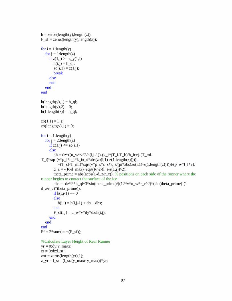
97

h = zeros(length(y),length(z));

F_sf = zeros(length(y),length(z));

for i = 1:length(y)

for j = 1:length(z)

if z(1,j) >= z_y(1,i)

h(i,j) = h_ql;

zo(i,1) = z(1,j);

break

else

end

end

end

h(length(y),1) = h_ql;

h(length(y),2) = 0;

h(1,length(z)) = h_ql;

zo(1,1) = l_s;

zo(length(y),1) = 0;

for i = 1:length(y)

for j = 2:length(z)

if z(1,j) <= zo(i,1)

else

dh = dz*((u_w*v^2/h(i,j-1))-(k_i*(T_i-T_b)/h_ice)-(T_mf-

T_i)*sqrt(v*p_i*c_i*k_i/(pi*abs(zo(i,1)-z(1,length(z)))))...

+(T_sf-T_mf)*sqrt(v*p_s*c_s*k_s/(pi*abs(zo(i,1)-z(1,length(z))))))/(p_w*l_f*v);

d_z = -(R-d_max)+sqrt(R^2-(l_s-z(1,j))^2);

theta_prime = abs(acos(1-d_z/r_c)); % positions on each side of the runner where the

runner begins to contact the surface of the ice

dhs = -dz*P*h_ql^3*sin(theta_prime)/((12*v*u_w*r_c^2)*(sin(theta_prime)-(1-

d_z/r_c)*theta_prime));

if h(i,j-1) == 0

else

h(i,j) = h(i,j-1) + dh + dhs;

end

F_sf(i,j) = u_w*v*dy*dz/h(i,j);

end

end

end

Ff = 2*sum(sum(F_sf));

%Calculate Layer Height of Rear Runner

yr = 0:dy:y_maxr;

zr = 0:dz:l_sr;

zor = zeros(length(yr),1);

z_yr = l_sr - (l_sr/(y_maxr-y_max))*yr;

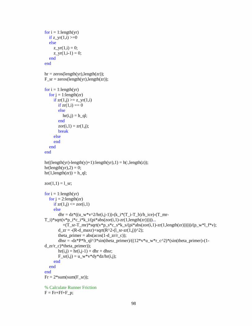
98

for i = 1:length(yr)

if z_yr(1,i) >=0

else

z_yr(1,i) = 0;

z_yr(1,i-1) = 0;

end

end

hr = zeros(length(yr),length(zr));

F_sr = zeros(length(yr),length(zr));

for i = 1:length(yr)

for j = 1:length(zr)

if zr(1,j) >= z_yr(1,i)

if zr(1,i) == 0

else

hr(i,j) = h_ql;

end

zor(i,1) = zr(1,j);

break

else

end

end

end

hr((length(yr)-length(y)+1):length(yr),1) = h(:,length(z));

hr(length(yr),2) = 0;

hr(1,length(zr)) = h_ql;

zor(1,1) = l_sr;

for i = 1:length(yr)

for j = 2:length(zr)

if zr(1,j) <= zor(i,1)

else

dhr = dz*((u_w*v^2/hr(i,j-1))-(k_i*(T_i-T_b)/h_ice)-(T_mr-

T_i)*sqrt(v*p_i*c_i*k_i/(pi*abs(zor(i,1)-zr(1,length(zr)))))...

+(T_sr-T_mr)*sqrt(v*p_s*c_s*k_s/(pi*abs(zor(i,1)-zr(1,length(zr))))))/(p_w*l_f*v);

d_zr = -(R-d_maxr)+sqrt(R^2-(l_sr-zr(1,j))^2);

theta_primer = abs(acos(1-d_zr/r_c));

dhsr = -dz*P*h_ql^3*sin(theta_primer)/((12*v*u_w*r_c^2)*(sin(theta_primer)-(1-

d_zr/r_c)*theta_primer));

hr(i,j) = hr(i,j-1) + dhr + dhsr;

F_sr(i,j) = u_w*v*dy*dz/hr(i,j);

end

end

end

Fr = 2*sum(sum(F_sr));

% Calculate Runner Friction

F = Fr+Ff+F_p;

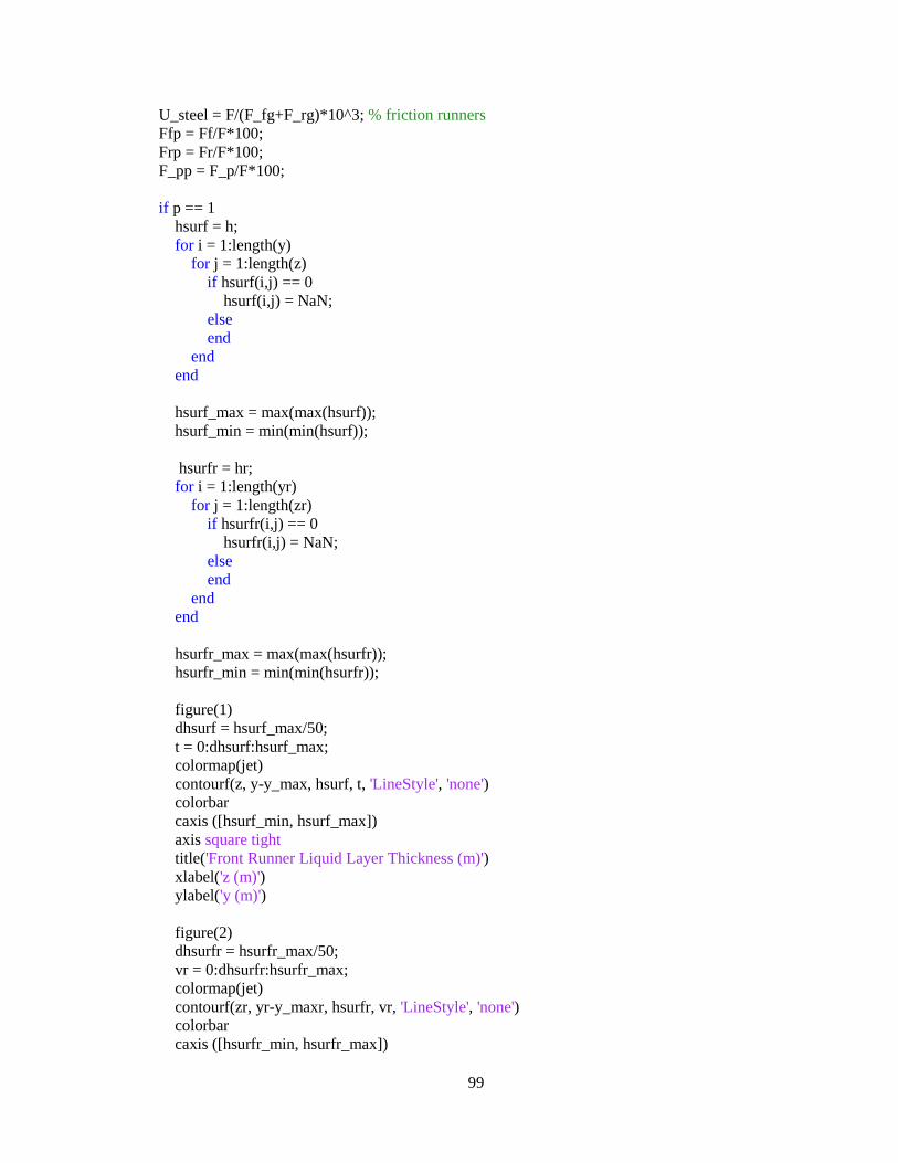
99

U_steel = F/(F_fg+F_rg)*10^3; % friction runners

Ffp = Ff/F*100;

Frp = Fr/F*100;

F_pp = F_p/F*100;

if p == 1

hsurf = h;

for i = 1:length(y)

for j = 1:length(z)

if hsurf(i,j) == 0

hsurf(i,j) = NaN;

else

end

end

end

hsurf_max = max(max(hsurf));

hsurf_min = min(min(hsurf));

hsurfr = hr;

for i = 1:length(yr)

for j = 1:length(zr)

if hsurfr(i,j) == 0

hsurfr(i,j) = NaN;

else

end

end

end

hsurfr_max = max(max(hsurfr));

hsurfr_min = min(min(hsurfr));

figure(1)

dhsurf = hsurf_max/50;

t = 0:dhsurf:hsurf_max;

colormap(jet)

contourf(z, y-y_max, hsurf, t, 'LineStyle', 'none')

colorbar

caxis ([hsurf_min, hsurf_max])

axis square tight

title('Front Runner Liquid Layer Thickness (m)')

xlabel('z (m)')

ylabel('y (m)')

figure(2)

dhsurfr = hsurfr_max/50;

vr = 0:dhsurfr:hsurfr_max;

colormap(jet)

contourf(zr, yr-y_maxr, hsurfr, vr, 'LineStyle', 'none')

colorbar

caxis ([hsurfr_min, hsurfr_max])

100

axis square tight

title('Rear Runner Liquid Layer Thickness (m)')

xlabel('z (m)')

ylabel('y (m)')

else

end

a_s = R^2*((pi/2)-asin(1-d_max/R))-(R-d_max)*sqrt(2*R*d_max-d_max^2); % m^2, area that

runner grips to resist lateral force

a_sr = R^2*((pi/2)-asin(1-d_maxr/R))-(R-d_maxr)*sqrt(2*R*d_maxr-d_maxr^2);

F_s = P*(a_s+a_sr); % N, ploughing force

toc

end