Embed Size (px)
Citation preview
Thermal Loading of Natural StreamsGEOLOGICAL SURVEY PROFESSIONAL PAPER 991
Thermal Loading of Natural StreamsBy ALAN P. JACKMAN and NOBUHIRO YOTSUKURA
GEOLOGICAL SURVEY PROFESSIONAL PAPER 991
UNITED STATES GOVERNMENT PRINTING OFFICE, WASHINGTON : 1977
UNITED STATES DEPARTMENT OF THE INTERIOR
CECIL D. ANDRUS, Secretary
GEOLOGICAL SURVEY
V. E. McKelvey, Director
Library of Congress Cataloging in Publication Data
Jackman, Alan P.Thermal loading of natural streams.
(Geological Survey Professional Paper 991)Bibliography: p. 38-39.Supt.ofDocs.no.: 119.16:9911. Thermal pollution of rivers, lakes, etc. I. Yotsukura, Nobuhiro, joint author. II. Title. III. Series: United States Geological
Survey Professional Paper 991. TD427.H4J3 363.6'1 76-608317
For sale by the Superintendent of Documents, U.S. Government Printing Office
Washington, D.C. 20402Stock Number 024-001-02959-6
CONTENTS
Page Page
Abstract____________________________ 1 One-dimensional model of excess temperature ContinuedIntroduction ______________________________ 1 Dan River near Eden, North Carolina, 1969 __________ 20Acknowledgments ____________________________ 2 Tittabawassee River near Midland, Michigan, 1969 ___ 22Equations for conservation of thermal energy _________ 2 North Platte River near Glenrock, Wyoming, 1970 ____ 23Heat transfer at the air-water interface ____________ 4 West branch of the Susquehanna River near Shawville,Analysis of natural temperature ____________________ 8 Pennsylvania, 1962 ____________________________ 26
Thermally homogeneous streams __________________ 9 Conclusions regarding one-dimensional modeling- ________ 27Thermal homogeneity of the Potomac River _________ 10 Two-dimensional model of excess temperature ________ ___ 27Prediction of natural temperature ______________ 13 Model for a steady uniform channel _____-____________ 27
One-dimensional model of excess temperature _________ 16 Model for a steady natural stream ____________ _ 28Preliminary considerations __________________________ 16 Applications to field data__________________________ 29Description of computational procedures ____________ 17 Summary regarding two-dimensional model __________ 36Results and discussion ____________________________ 18 Summary and conclusions ________________ _______ 37White River near Centerton, Indiana, 1969 __________ 18 References cited __________________________________ 38Fenholloway River near Foley, Florida, 1969________ 20
ILLUSTRATIONS
Page
FIGURE 1. Temporal variations of water temperature at five positions in a hypothetical channel with doubled depth (a = 2) _______ 102. Temporal variations of water temperature at five positions in a hypothetical channel with halved depth (a = ¥2) ________ 103. Sketch of the Potomac River study reach below Dickerson Power Plant, Maryland _______________________ ___ n4. Transverse profiles of water temperature at selected sections, the Potomac River below Dickerson Power Plant, Maryland,
March 11, 1969______________________________________________________________ 125. Longitudinal profile of natural water temperature near right bank, the Potomac River below Dickerson Power Plant,
Maryland, March 11, 1969___________________ _____________________________________ 126. Longitudinal profile of natural water temperature near right bank, the Potomac River below Dickerson Power Plant,
Maryland, May 14, 1969____________________ _____________________________________ 127. Transverse profile of natural water temperature at section 1, the Potomac River above Dickerson Power Plant, Maryland,
March 11-12, 1969 ____________________________________________________ ___________________ 138 Comparison of observed and calculated natural water temperatures at section 4, the Potomac River below Dickerson
Power Plant, Maryland, March 1969 ___________ ____________________ ________________ 139. Comparison of observed and calculated natural water temperatures at section 4, the Potomac River below Dickerson
Power Plant, Maryland, May 1969 _____________ _____________________________________ 1310. Comparison of observed and calculated natural water temperatures, the Potomac River below Dickerson Power Plant,
Maryland, 1969, and the Riverside Inlet Canal near Greeley, Colorado, 1970 ___________ ______________ 1511. Attenuation of remaining excess heat with distance downstream from heat discharge site __ __________________ 1712. Sketch of study reaches, I _____________________ _____________________________________ 1913. Sketch of study reaches, II_____________________ _____________________________________ 1914. Comparison of observed and calculated water temperatures, the White River near Centerton, Indiana, 1969 _ 2015. Comparison of observed and calculated water temperatures, the White River near Centerton, Indiana, 1969 __________ 2016. Comparison of observed and calculated water temperatures, the White River near Centerton, Indiana, 1969 __________ 2017. Temporal variation of natural and heated water temperatures, the White River near Centerton, Indiana, 1969 ________ 2118. Comparison of observed and calculated water temperatures, the Fenholloway River near Foley, Florida, 1969 _________ 2219. Comparison of observed and calculated water temperatures, the Fenholloway River near Foley, Florida, 1969 ______ 2320. Comparison of observed and calculated water temperatures, the Fenholloway River near Foley, Florida, 1969 ________ 2421. Comparison of observed and calculated water temperatures, the Fenholloway River near Foley, Florida, 1969__ _ ____ 2422. Comparison of observed and calculated water temperatures, the Fenholloway River near Foley, Florida, 1969 ___ 2423. Comparison of observed and calculated water temperatures, the Fenholloway River near Foley, Florida, 1969 _ ______ 2524. Comparison of observed and calculated water temperatures, the Dan River near Eden, North Carolina, 1969__________ 2525. Comparison of observed and calculated water temperatures, the Dan River near Eden, North Carolina, 1969_________ 2526. Comparison of observed and calculated water temperatures, the Dan River near Eden, North Carolina, 1969___-__- _____ 2527. Comparison of observed and calculated water temperatures, the Tittabawassee River near Midland, Michigan, 1969 _ _ 2628. Comparison of observed and calculated water temperatures, the Tittabawassee River near Midland, Michigan, 1969 ___ 26
IV CONTENTS
Page
FIGURE 29. Comparison of observed and calculated water temperatures, the North Platte River near Glenrock, Wyoming, 1970 __ 2630. Comparison of observed and calculated water temperatures, West Branch of the Susquehanna River near Shawville,
Pennsylvania, 1962 ______________________ _____________________________________ 2731. Sketch of a two-dimensional natural stream and its stream-tube flow system ____ __ __ _ ___ _ _ ____ _ _____ ____ 2932. Concurrent transverse distributions of dye concentration and excess temperature, the Potomac River below Dickerson
Power Plant, Maryland, March 1969 ____________ _ ___ ____ _ __ __ ______ _ ___ _ __ __ ___________ ____ ____ 3033. Temporal variations of surface heat dissipation coefficient and source excess temperature, the Potomac River below Dick
erson Power Plant, Maryland, March 1969 ___ __ _ _ _ ________ _ _____ _ ____ _ ______ _ _____________ _ __ 3034. Comparison of observed and calculated transverse temperature distributions, the Potomac River below Dickerson Power
Plant, Maryland, March 1969 _______________ _____________________________________ 3135. Temporal variations of surface heat dissipation coefficient and source excess temperature, the Potomac River below Dick
erson Power Plant, Maryland, May 1969 __ _______ __________________ __________________ 3236. Comparison of observed and calculated transverse temperature distributions, the Potomac River below Dickerson Power
Plant, Maryland, May 1969 _________________ _____________________________________ 3337. Comparison of observed and calculated transverse temperature distributions, the Potomac River below Dickerson Power
Plant, Maryland, May 1969 _________________ _____________________________________ 3438. Comparison of observed and calculated transverse temperature distributions, the Potomac River below Dickerson Power
Plant, Maryland, October 1969 _______________ _____________________________________ 3439. Comparison of observed and calculated transverse temperature distributions, the Potomac River below Dickerson Power
Plant, Maryland, October 1969 _______________ _____________________________________ 3540. Comparison of observed and calculated transverse temperature distributions, the Potomac River below Dickerson Power
Plant, Maryland, October 1969 _ _____ _ ___ ___ _ _ _ __ __ _______ _________________ __ ______ __ _ ___ _ 3541. Comparison of observed and calculated transverse temperature distributions, the Dan River near Eden, North Carolina,
April 1969 ____________________________ _____________________________________ 3642. Comparison of observed and calculated transverse temperature distributions, the North Platte River near Glenrock,
Wyoming, January 1970 ___ _______________ _____ __________________ _____________ 36
TABLES
Page
TABLE 1. Temporal variation of hypothetical natural temperature under freezing conditions, the North Platte River near Glenrock, 19Wyoming, January 28-29, 1970 ____________________________________________________
2. Cross-sectional average hydraulic parameters, the Potomac River below Dickerson Power Plant, Maryland, March 1969- _ 30
THERMAL LOADING OF NATURAL STREAMS
By ALAN P. JACKMAN and NOBUHIRO YOTSUKURA
ABSTRACT
The impact of thermal loading on the temperature regime of natural streams is investigated by mathematical models, which de scribe both transport (convection-diffusion) and decay (surface dissi pation) of waste heat over 1-hour or shorter time intervals. The models are derived from the principle of conservation of thermal energy for application to one- and two-dimensional spaces.
The basic concept in these models is to separate water temperature into two parts, (1) excess temperature due to thermal loading and (2) natural (ambient) temperature. This separation allows excess tem perature to be calculated from the models without incoming radia tion data. Natural temperature may either be measured in pro totypes or calculated from the model. If use is made of the model, however, incoming radiation is required as input data.
In order to formulate a linear decay model for excess temperature, the equations for back radiation, evaporation, and conduction, de rived from the Lake Hefner study of U.S. Geological Survey, are linearized with reference to an arbitrary base temperature. It is shown that the resulting surface dissipation coefficient is predomi nantly influenced by wind speed and the mass-transfer coefficient of evaporation.
For one-dimensional problems, the transport of excess tempera ture is solved by the Lagrangian convection model of traveling with an average heated water packet. In two-dimensional problems, a steady-state diffusion model is combined with the one-dimensional decay model. Longitudinal dispersion is neglected in both transport models.
Comparison of observed and calculated temperatures in seven natural streams shows that the models are capable of predicting transient temperature regimes satisfactorily in most cases. Mass- transfer coefficients of evaporation in streams are much higher than those commonly used for long-term calcualtions in a lake. Factors such as ground-water accretion, abrupt changes in thermal loading, and unstable atmospheric conditions are found to have significant impacts on water temperature regimes.
The dissipation of excess heat in natural streams is a gradual process frequently extending over a long downstream distance. For five out of the seven study reaches, the remaining excess heat at a point nearly 30 kilometres downstream was more than 50 percent of the initial thermal load.
INTRODUCTION
The impact of thermal loading (waste heat dis charge) on temperature regime of a natural water body is the basic physical information that is required for meaningful assessment of water-quality changes in duced by such waste discharges.
The Geological Survey has been engaged for more than 20 years in the study of thermal loading as an outgrowth of the study of evaporational water losses in lakes. The results of the earlier studies have been
published in papers by Harbeck (1953), Harbeck, Koberg, and Hughes (1959), Messinger (1963), Har beck, Meyers, and Hughes (1966), and Harbeck (1970). These studies used the energy-budget equation derived from the Lake Hefner study (Anderson, 1954) and in vestigated daily- or weekly-average (long-term) ther mal regimes of a few western lakes and a couple of natural streams.
Toward the end of 1968, the extension of thermal loading studies to natural streams was deemed urgent in view of the mounting concern about thermal pollu tion caused by power generation (Parker and Krenkel, 1969). At the same time, keen interest was shown in the collection of synoptic data from thermally loaded streams covering a wide range of meterologic and hy draulic conditions.
Accordingly, the Geological Survey, in cooperation with the Atomic Energy Commission (now the Energy Research and Development Administration), under took a 1-year program of data collection in six natural streams that were thermally loaded and located in dif ferent regions of the country. Briefly, a stream survey consisted of measuring water temperature, meteoro- logic variables, discharges, and channel geometries at several cross sections downstream from the heat source for a duration of 24 hours. In many streams, two to three surveys were conducted during the year to evaluate seasonal thermal patterns. All survey works were completed between February 1969 and January 1970. In addition, the thermal data of the Susquehana River collected by the Geological Survey in 1962 were considered worthy of reexamination and included in the data set of the present report.
Examination of these stream data revealed that, even though the energy-budget equation adequately describes the heat exchange at the air-water interface, it is not suitable for describing the heat transport. In order to predict natural stream phenomena in terms of hourly (short-term) variations, the equation for con servation of thermal energy must be derived and solved with due considerations given to the transport aspect as shown by recent studies such as Edinger and Geyer (1965), Jaske (1969), Morse (1970), and Harle- man (1972) among others.
In solving the thermal energy equation, further-
THERMAL LOADING OF NATURAL STREAMS
more, some of the customary models and assumptions had to be reexamined. For example, the steady-state exponential decay law predicts that the excess temper ature decreases exponentially with increasing down stream distances. In view of highly variable thermal loading patterns and meteorologic conditions in proto types, such a simple model could not accommodate short-time or equivalently short-distance phenomena (Jackman and Meyer, 1971). Another example is the equilibrium temperature that is used to calculate the surface heat dissipation coefficient. It is an approxima tion acceptable only for daily or weekly averages but not for hourly averages (Jobson, 1973a; Yotsukura and others, 1973).
The new approach consists of combining the convec- tive diffusion equation of heat transport with a linear ized equation for dissipation of excess heat at the air- water interface (Jackman and Meyer, 1971; Jobson, 1973a; Jobson and Yotsukura, 1973). The approach to surface heat dissipation is Lagrangian in the sense of following average water particles downstream. The dissipation coefficient is calculated with reference to the daily average ambient temperature upstream from the heat source. In addition, a two-dimensional diffu sion approach was incorporated into the analysis to facilitate the definition of the mixing zone (Yotsukura, 1972).
The present report describes the final analysis of the thermal data by the analytical models evolved in the
last few years and discussed in the above-mentioned papers. The original thermal data and detailed de scription of field conditions will be presented by a com panion paper, which is herein referred to as the Data Report. The following tables describe the measurement units used herein.
ACKNOWLEDGMENTS
The present model study benefited greatly from con tributions from a number of specialists in the U.S. Geological Survey. The authors acknowledge, in par ticular, E. J. Pluhowski, E. F. Hollyday, F. A. Kilpat- rick, J. F. Bailey, and R. L. Cory for their valuable con tributions throughout the study. The authors also would like to acknowledge cooperations generously given by W. F. Weeks and C. M. Keeler of the Cold Regions Research and Engineering Laboratory, Han over, N.H., in conducting the thermal study for the North Platte River.
Coordination of the data collection program of this scale was certainly not a simple task. Credit is due E. L. Meyer, whose skill and devotion applied to the task was a major factor in the successful completion of the field work.
EQUATIONS FOR CONSERVATION OF THERMAL ENERGY
Water temperature expresses the thermal energy of
Conversion of units between SI and conventional systems for basic quantities[This table is based on (1) National Bureau of Standards, 1972, The International System of Units (SI): NBS Special Publication 330. (2) National Physical Laboratory, 1966, Changing
to the metric system: H.M.S.O., London. (3) Baumeister, T., 1958, Mechanical Engineer's Handbook: McGraw-Hill Book Co., Inc., New York]
Quantity
Length
Area
VolumeMassForce
Energy Power
SI units Conventional units Conversion
Metre _______________ Foot__________Kilometre ____-______ Mile______ Square metre ___________ Square foot ___.Square kilometre.---______ Square mile ______Cubic metre ___________ Cubic foot _____.Kilogram __________ Pound_______.Newton ___________ Kilogram-force _-
Pound-force ___. Joule _________________ Calorie _______.Watt ___________ Calorie per second
1 m =3.281 ft 1 km =0.6214 mi 1 m2 =10.76 ft2 1 km2 = 0.3861 mi2 1 m3 =35.31 ft3 1 kg =2.205 Ib
N =0.1020 kg N =0.2248 Ib J =0.2388 cal W= 0.2388 cal-s-1
1 ft =0.3048 m 1 mi =1.609 km 1 ft2 =0.09290 m2 1 mi2 =2.590 km2 1 ft3 =0.02832 m3 1 Ib =0.4536 kg 1 kg =9.807 N 1 lb =4.448 N 1 cal =4.187 J leal-8*= 4.187 W
Conversion of units between SI and conventional systems for derived quantities[Quantities represent those commonly used in thermal studies and conversions are given at the magnitudes observed under normal climatic conditions]
Quantity
Water density ____ Wind speed______ Atmospheric pressure Specific heat of water
SI units Conventional units
Latent heat of vaporization Radiation and heat flux _.
Mass transfer coefficient of evaporation.
Stefan Boltzman constant of black body radiation.
Kilogram per cubic metre ___ Pound per cubic foot _ _____Metre per sec __________ Mile per hour-_________Newton per square metre __ Millibar ____ __ __Joule per kilogram per Calorie per gram per degree
degree kelvin. Celsius.Joule per kilogram ________ Calorie per gram _ __Watt per square metre _____ Calorie per square centimetre
per hour. Kilogram per metre Gramme per square centimetre
per newton. per hr per mile-per-hrper millibar.
Watt per square metre per Calorie per square centimetre(degree kelvin).4 per min per (degree Kelvin).4
Conversion
1,000 kg-m-3 = 62.43 Ib-ft"8 1 m-sec-i =2.237 mile-hr1 105 N-m-2 = 103 mb 4,187 J-kg-1 -K-1 = 1 cal-g'1 -C'1
2,495 103 J kg'1 =596 cal g'1 1,000 W-m-2 =85.97 cal-cnr2
hr1 2-10-8 kg-m-i-N-1
=3.218-lO^g-cnr2 -mile^-mb'1
5.67-10-8 W-m-2 -K^=8.14-10-11 cal-cm'2 mm'1 -IT*
EQUATIONS FOR CONSERVATION OF THERMAL ENERGY
a water body. In natural conditions the thermal energy may be considered equivalent to the internal energy. In order to derive an equation for thermal energy bal ance, one starts with the First Law of Thermodynam ics, which says that the increase in total energy con tent of a body is the sum of all heat inputs to the body minus the amount of work that is performed by the body. When one subtracts from the equation of total energy balance those parts that are related to mechan ical energies, namely, kinetic and potential energies, the differential equation for conservation of thermal energy is obtained as (Pai, 1956)
(1)
where p is water density, Cp is the specific heat of water at constant pressure, T is temperature, t is time, K is the thermal conductivity, <I> is the rate of heat produc tion by viscous dissipation of mechanical energy, and S is the net heat input from sources and sinks.
In equation 1, the operator D/Dt is the substantial derivative, or
D d d(2)
where ux , vy , and vz are velocities in the respective coor dinate directions. The symbol V2 designates the Lapla- cian operator or a sum of the three second-order partial derivatives with respect to x, y, and z. Equation 1 as sumes that water is incompressible even though its density may vary in space and time. Thus, any change in energy content due to volume expansion or compres sion is neglected. The equation also represents instan taneous balance of thermal energy within an infinites imal body of water.
Since most applications of the thermal equation in natural water deal with turbulent flows, equation 1 needs to be averaged over a time scale appropriate for a turbulent flow. The procedure, which is based on the Reynolds' classic averaging method (Hinze, 1959), yields the following equation:
DT d , dT d ,, dT. d(3)
Here T represents time-averaged temperature, S rep resents time-averaged heat sources and sinks, and the symbols kx , ky , and kz are turbulent thermal diffusion coefficients in the respective directions. In comparing equation 3 with equation 1, note that the molecular conduction term, KV2T", and the viscous dissipation term, <I>, are neglected after averaging, because these are quite small relative to other averaged terms. For example, for every 1-metre drop in the surface eleva tion of a uniform stream, this much potential energy is
converted through viscous dissipation to thermal energy. This is equal to a heat gain of 9.807 joules per kg of water and corresponds to a temperature rise of only 0.0023°C. The turbulent diffusion terms, on the other hand, appear in equation 3 as lump-sum expres sions for the correlation that exists between the devia tions of instantaneous velocities and temperature from time-averaged values. The symbols vx , vy , and vz in the substantial derivative, D/Dt, are now all time-aver aged velocities.
Owing to the three-dimensional nature of equation 3, its solution is often difficult. In order to reduce its dimension, equation 3 may be integrated over the local depth as shown by Leendertse (1970), Prych (1970), and Holley (1971). Assume that they coordinate is di rected vertically upward. By means of Leibnitz's rule of integration and kinematic boundary conditions appro priate for a natural water body, equation 3 is inte grated to the following equation:
dYT ,dYvxTdt dx dz
dT. d
The symbol Y designates local depth, T is depth- averaged temperature, vx and vz are depth-averaged velocities, and Kx and Kz are turbulent thermal- dispersion coefficients. The dispersion term in equation 4 consists of two parts. One is the contribution from the correlation between the local deviations of velocities and temperature from depth-averaged values. This correlation is expressed by a gradient-type dispersion term following Taylor's (1954) model in a steady uni form flow. An additive part is contributed by depth averaging of the turbulent diffusion term of equation 3. The source-sink term is now defined by YS where S is the depth-averaged value. The symbol H defines boundary heat influx normal to the water surface and Hbot defines one normal to the channel bottom. These terms are introduced into equation 4 by the boundary condition which assumes that incoming heat flux is transported inward by turbulent diffusion without any storage at the boundary.
For a natural stream, where the width is small rela tive to longitudinal distances, it is often convenient to have one-dimensional thermal equations. Equation 4 may now be integrated over the channel width, using the same techniques as used in deriving equation 4. The result is
dAT dAVT HT~ "T" dt ox
d~a~dx
dT~a~'ox
AS WH 7T ~r 77~
pCp pC>pC
In equation 5, A is the cross-sectional area, T is the
THERMAL LOADING OF NATURAL STREAMS
cross-sectional average temperature, V is the cross- sectional average longitudinal velocity, K is the cross- sectional average thermal dispersion coefficient, and S is the cross-sectional average source sink. The symbols H and #hot are width-averaged surface flux and bottom flux, respectively, while W designates the surface width at the cross section.
Even though the details of derivations of the above equations are omitted in the present report, examina tion of various references shows that these equations are general and most suitable for use in natural water bodies where flows may be transient and boundaries complex. In deriving these equations, no assumptions are made as to the steadiness or uniformity of flow. On the other hand, various diffusion and dispersion terms are added as the averaging progresses from one stage to the next. These terms are introduced as an analogy to gradient-type molecular diffusion. Although some of these diffusive terms have been verified as workable approximations by experiments, notably in a steady uniform flow, one must remember that the expressions for dispersion and diffusion are definitions rather than established physical laws. Fortunately diffusive trans port is normally small relative to average-velocity (convective) transport and may even be neglected under certain conditions.
HEAT TRANSFER AT THE AIR-WATER INTERFACE
The mechanics of heat transfer at the flow bound aries of a natural water course is important in thermal loading problems, because the excess thermal energy possessed by water is ultimately dissipated to the air and the soil through such transfers. It is known that heat transfer at the water surface is one of the major factors in determining water temperature under both natural and thermally loaded conditions. In compari son, heat transfer through the streambed is normally small, except possibly in extremely shallow streams flowing over solid beds of rock (Brown, 1972). Moreover, there is very little information currently available on this transfer process. For these reasons, the soil-water interface transfer will be neglected hereafter.
Heat transfer at the air-water interface may be de scribed most conveniently with reference to the one- dimensional thermal equation, because the same surface-transfer equations are applied to the more complex two- and three-dimensional equations. The left side of equation 5 may be simplified by substitut ing the continuity equation of water. Also the source term, S, and the longitudinal dispersion term, KAdTI dx, are neglected. Equation 5 is then reduced to
dT_ dT H dt dx pCpY
(6)
The depth, Y, is defined by AIW according to equa tion 5.
Four mechanisms have been identified as contribut ing to the net heat flux, H. They are shortwave radia tion, longwave radiation, evaporation, and conduction. The largest of these terms is the shortwave radiation, which may assume values as large as 1,200 watts -nr2 . It always contributes a positive component to H since essentially no shortwave radiation is emitted by the water. Incoming shortwave and longwave radiation differ significantly from other components in that they do not depend in any way on water temperature. Moreover, the shortwave radiation has a well-defined dependence on time of day through the sun angle, whereas all other terms, while varying in a somewhat random fashion with time in response to variables such as wind speed, have no deterministic dependence on time.
Outgoing longwave radiation, evaporation, and con duction all depend on the water temperature. Because of the complex nature of some of the dependencies, these terms cause equation 6 to be nonlinear. They do not depend directly on the time, although evaporation and conduction depend on such factors as wind veloc ity, atmospheric stability, and humidity, which vary with time. The maximum values of these components are considerably smaller than that for incoming shortwave radiation.
The fact that incoming shortwave and longwave radiation do not depend on water temperature enables one to remove these components from the thermal equation through a transformation of the temperature variable. Suppose there was no waste heat discharged into the stream. The temperature, Tn , which would exist under natural conditions is described by the same equation as equation 6 but with H depending on t and Tn , or
dTn dTn _ H(Tn ,t) dt dx pCpY (7)
It is assumed that the coefficients of equations 6 and 7, such as V and Y, are not affected by thermal condi tions. If the excess temperature, Te , is defined as the difference between T and Tn , then, subtracting equa tion 7 from equation 6,
dTe v dTe _H(T,t}~H(Tn ,t} dt dx pCpY (8)
The net flux, H(T,t\ may be divided into four compo nents,
HEAT TRANSFER AT THE AIR-WATER INTERFACE
H(T,t)=Hr(t)-Hb (T) -He (T,t}-Hc (T,t\ (9)
where Hr is the net incoming radiation, both longwave and shortwave, which actually crosses the air-water interface unreflected, Hb is the back radiation (longwave radiation emitted by the water), He is the heat flux due to evaporation of water, and Hc is the heat flux due to conduction from the water into the atmosphere. Note that only Hr is independent of T\ therefore, if equation 9 is substituted into equation 8, iheHr (t) from the two terms will cancel, and equation 8 is written as
^dTe dTe dt V dx (10)
PCPY
This is a considerable simplification, as equation 10 can be solved without knowing the total incoming radiation. Total incoming radiation, in addition to being a large term of considerable variability, is a quantity that is not now being continuously measured and reported by any agency. For each application it must, therefore, be measured, and this requires ex pensive equipment that is difficult to maintain and calibrate.
In addition to simplifying the modeling problem, ex cess temperature is a variable of considerable impor tance in studying the impact of man on the stream environment. In the case of a discharge of waste heat, the heat added to the water will increase the internal energy of the water, thus increasing the water temper ature. Thermodynamics dictates that the increase in temperature resulting from a waste discharge is a nearly linear function of the amount of heat added to a unit mass of the water. This increase in temperature is the excess temperature, Te . Thus, a waste heat dis charge may be thought of as a source of excess tem perature.
Just as the excess temperature at the point of dis charge is a measure of the amount of heat added at that point, the excess temperature at a down-stream point is a measure of the amount of the waste heat that still remains. The solution of equation 10 describes the excess temperature as a function of space and time and, thus, gives an idea of how much of, and to what degree, the stream is affected.
Calculations involving excess temperature are not limited to waste heat discharges. For instance, the re covery of subnormal stream temperatures resulting from cold water releases below impoundments may be estimated using the excess temperature approach. In
this case, excess temperatures will be negative owing to the fact that the stream has lower energy content than it would under natural conditions.
In order to calculate the excess temperature using equation 10 it will be necessary to know Te at some point as a function of time, for example, a boundary condition. This may be specified at the point of dis charge, in the case of a waste heat discharge, by divid ing the rate of discharge of waste heat by the product of the density, the specific heat, and the volumetric rate of flow of waste water into the stream. It is also possi ble, in those cases where the stream mixes rapidly, to measure the difference between the temperature at a point just upstream of the discharge point and the temperature of the stream once fully mixed below the discharge point. Both of these approaches assume that the temperature just upstream of the discharge is the natural temperature. If this is not the case, it will be necessary to estimate the natural temperature at the upstream point.
The solution of equation 10 for excess temperature requires expressions for the heat exchange due to out going longwave radiation, evaporation, and conduc tion. In the case of evaporation and conduction mecha nisms, there are a number of expressions available. Much room for improvement in these expressions exists. The models discussed here are among the most frequently used.
The longwave or "thermal" radiation emitted by a body is known to be related to the temperature of a body by the Stefan-Boltzmann equation:
Hb =a- (T+273.16)' (11)
-2 07where o-=5.67-10"8 watts -m" -K is the Stefan- Boltzmann constant, e is the total hemispherical emis- sivity, T is temperature of the body in degrees Celsius, andHb is given in units of watts-m"2 . Anderson (1954) reported that for natural waters the emissivity is es sentially independent of the dissolved-solid concentra tion and temperature. Emissivity was also found to be independent of the suspended sediment load, but an oil layer on the water surface significantly reduces emis sivity. Anderson concluded that for oil-free natural waters the emissivity is 0.970±0.005.
In spite of extremely precise formulation provided by equation 11, there are still inaccuracies that may at tend its use with natural water bodies. These errors arise because of errors in the temperature. Most longwave radiation emitted by a water surface is pro duced in the first 100 ^m below the water surface (McAlister and McLeish, 1969). Ewing and McAlister (1960) found that the temperatures within this layer
THERMAL LOADING OF NATURAL STREAMS
may differ significantly from that temperature which would be measured with the smallest conventional temperature measuring device placed as close to the water surface as possible. The true surface tempera ture is generally found to be lower than the bulk water temperature. Thus, calculations of back radiation based on bulk temperature will overestimate the ac tual back radiation. The error in calculated back radia tion will usually be less than 3 percent, because the surface is usually less than 2°C (Celsius) cooler than the bulk. Equation 11, with the temperature measured near the surface using conventional thermometry, should give a satisfactory estimate of back radiation for most purposes.
Evaporation contributes to the heat flux at the air- water interface in two ways. First, in order for water in the liquid state to enter the gaseous state an amount of energy, the latent heat of vaporization must be added. This energy, approximately 2.5-10 joules per kg of water, must be supplied from the water body. Thus, the water body loses energy by the evaporation process. In addition, some mass of water is lost, and this repre sents a decrease in the total energy of the system. This term does not have any effect on the energy content per unit mass and becomes important only in cases where a change in the mass of the system is significant. It will be ignored in this work.
The rate of evaporation from a water surface is re lated to the rate at which water vapor may be transfer red away from the interface. The transport process in volved is a turbulent diffusion process. If the air far away from the interface has a lower partial pressure of water vapor than the air very near the interface, then a gradient for diffusion will exist. Note that this gra dient may be reversed and condensation may occur, causing an influx of energy to the water body. The partial pressure of water vapor at the interface is the saturation vapor pressure for water at the temperature of the interface that will be approximated by the bulk water temperature.
The diffusive flux of water vapor away from the interface may be expressed as
RT,kHf)
dy(12)
where R is the gas constant, T2 is the air temperature, &H2 o is the turbulent diffusivity of water vapor in air, and PH2Q is the vapor pressure. The diffusivity is known to be a function of wind velocity. If the wind velocity profile follows a logarithmic form, it may be shown (Priestly, 1959) that at a given distance, y2 , above the surface
K2V 2
(13)
where K is the von Karman constant taken to be 0.40,17 is the turbulent Schmidt number, v2 is the wind speed at elevation y2 , and y0 is a constant known as the roughness. This expression is valid only during periods of neutral atmospheric stability, but it shows a direct proportionality of £ H2 o on wind speed.
Among many existing models of evaporation, the most commonly used are the mass transfer models, which are also called Dalton-type equations. These models recognize that evaporation is proportional to the vapor pressure difference and that the coefficient of proportionality is a function of wind speed. Marciano and Harbeck (1954) and Harbeck (1962) studied them carefully and found that the following simple formula gives adequate results for lakes and reservoirs when all quantities are time averaged over a period of 1 day or longer:
E=Nv2 (ps -p2 (14)
where N is the mass transfer coefficient, v 2 is the wind speed at some elevation (usually two metres), ps is the saturation vapor pressure of water at the temperature of the surface, and p2 is the partial pressure of water vapor at the same elevation as used for wind speed.
Harbeck (1962) found that the value of N varies with the surface area of a water body according to
Af=3.42-10" (15)
where A s is the surface area in square meters andAf is given in units of kg-m^-newton"1 . Taking a typical stream to have an effective surface area for evapora tion of 1,000 m2 , one finds a value of N=2.42-10~8 kg m' 1 newton" 1 .
It has been recognized for some time that the value of N may not be a constant but may depend on wind direction and atmospheric stability. While these fac tors may not be important when using data averaged over long periods of time, they may be very important when using hourly data. Brutsaert and Yeh (1970) showed that rather than N depending on the area of a water body, it should depend on fetch. They find that Af should be proportional to the fetch to the -0.25 power. The average fetch length will depend on wind direction for all but circular bodies, and it is very difficult to assess this factor for streams.
There is an increasing interest in the effect of at mospheric stability on the mass transfer process. It is generally believed that under unstable atmospheric conditions the rate of mass transfer will be increased owing to the existence of buoyancy-driven natural con vection currents. And under stable conditions, the value of the eddy diffusivity will be reduced, reducing the rate of mass transfer. On the basis of the Lake
HEAT TRANSFER AT THE AIR-WATER INTERFACE
Mead studies, Harbeck, Kohler, Koberg, and others (1958) recommended a stability dependent form for the mass transfer coefficient:
7V=1.04-l(r8 [l-0.03(T2 -T)], (16)
where T is surface water temperature in °C, T2 is the air temperature in °C, and TV is given in units of kg-m'^newton" 1 .
The evaporative heat flux may be calculated directly from the flux of water vapor, E, using any of the above expressions. This is done by multiplying the flux by the latent heat of vaporization, A., so that
H=\E. (17)
A commonly used value of A. is 2495 103 joules per kg. The conductive heat flux has generally been calcu
lated from the evaporative heat flux, as was first suggested by Bowen (1926). It may be shown that if the vertical fluxes of water vapor and heat are independent of distance from the surface, and if the turbulent dif- fusivities of heat and mass are identical, then
H=BH*nd (18)
B=6.1'W*'P(T-Tz )(p8 -p2 Y1 , (19)
where B is the Bowen Ratio and P is the atmospheric pressure in newtons m"2 . Temperatures are in degrees Celsius, and vapor pressures are expressed in newtons-m"2 .
Equations 11, 17, and 18, in conjunction with equa tions 14 and 19, describe all the fluxes appearing in the one-dimensional excess temperature model, equation 10. The same fluxes are also needed for the two- dimensional excess temperature model.
The one-dimensional excess temperature equation can now be solved, provided that necessary initial and boundary conditions are specified and that the wind speed and partial pressure of water vapor at the 2-m level are known. Unfortunately, all the flux terms ex cept the conductive flux, Hc , are nonlinear functions of water temperature, T. The back radiation depends on the fourth power of water temperature according to equation 11. The evaporative flux depends on the sat uration vapor pressure of water, which is an exponen tial function of water temperature,
ps = 610-exp[l9.7071-5383.2-(T+273.16)'1 ] (20)
where ps has units of newtons m"2 and T is in degrees Celsius.
Linearized approximation of Hb and He may be ob tained by expanding equations 11 and 17 as Taylor series about an arbitrary base temperature, Tb , and truncating all terms of second order and higher. Sub tracting the expressions for Tn from those for T, the following equations are obtained:
Hb (T) = Hb (Tn ) + 4<re(Tb + 273.16)3 -Te
He (T) = He (Tn ) + 5383.2
+ 273.1 6) 2 -T, and
(T
(21)
(22)
HC (T} = Hc (Tn ) + e.MO^-PAM^T, . (23)
Substituting equations 21, 22, and 23 into equation 10, the one-dimensional excess temperature equationis
dTe UTedt
ydx
(24)
where U, defined as the heat dissipation coefficient, closely resembles the conventional engineering heat transfer coefficient and is given by
U = 4o-e(T6 +273.16)3 + \Nv2 [5383.2 -ps (Tb ) (Th
+273.16)'2 + 6.M(T*-P] . (25)
For most computations, a constant temperature may be used as Tb so long as it does not deviate excessively from natural temperature Tn (Jobson, 1973a, Yotsuk- ura and others, 1973). Two other coefficients for sur face heat dissipation may be defined in conjunction with U. These are
U and
T,=U
(26)
(27)
In solving equation 24, note that the left side is iden tical to the one-dimensional substantial derivative, DTJDt. By definition, it describes the time variation of Te of a particular water packet. Equation 24 can be simplified by interpreting it in the Lagrangian sense of following the water packet moving with velocity V. The travel time, T, may be defined such that
x = + x
and
t = T + t0 ,
(28)
(29)
THERMAL LOADING OF NATURAL STREAMS
where x0 and t0 are given values of x and t at r=0. Equation 24 is, thus, reduced to an ordinary differen tial equation with T as the single independent variable:
dr.L_
Td(30)
The analytical solution to this equation is easily ob tained as
7>Teo exp(-rldT'), (31) 0 T«
where Teo is an initial excess temperature at r=0.Note that the time constant, rd , depends on U, which,
in turn, depends on u2 and Tb as shown in equation 25. Even if Tb may be assumed constant, u2 , the 2-m wind speed, varies rapidly with time. Thus, rd is a function of time. It is often desirable to predict downstream tem perature for a travel time longer than the interval for meteorological observation; for example, employ equa tion 31 for a travel time of 24 hours using wind-speed data collected at hourly intervals. In cases such as this, the travel time must be segmented into periods, AT, equal in length to the period for a wind speed observa tion, and the integral in the exponential term of equa tion 31 becomes a summation of Ar/rd over the travel time T. This segmentation causes the calculations to have a serial character much as would a direct nu merical integration of equation 10, although less te dious and free of convergence problems. Yotsukura, Jackman, and Faust (1973) have shown that the linearization results in appreciable errors when the excess temperature is larger than 10°C. In such cases the numerical integration of equation 10 would be an attractive alternative.
Recapitulating on the various heat exchange equa tions introduced in this section, it is evident that the description of evaporation processes needs further im provement. Equation 14 was adopted in this report on the basis of proven practical usefulness, but it is an empirical equation. It will be very attractive to develop equations that do not depend on water temperature. The aerodynamic models of estimating evaporation have an advantage over the mass transfer models in that they do not contain empirical coefficients such as the mass transfer coefficient and that they accommo date more theoretically sound description of evapora tion processes. Jobson (1973b) and Pierson and Jackman (1975) reported progress made in this course of approach.
The total incoming radiation, Hr , was removed from the energy equation when equation 10 was derived for excess temperature. This heat flux is important when the natural temperature needs to be estimated. This quantity is best determined experimentally. When ex
perimental determination is not possible, however, there are models for both the longwave and shortwave incoming radiation. Sellers (1965) described a number of models for both fluxes. Koberg (1964) presented a method for estimating longwave radiation, and Ander- son (1954) presented a model for determining the re flectivity of a natural water surface. These models should only be employed where direct measurement of incoming radiation is not feasible.
It is also worth noting that, in spite of nonlinear relations between heat fluxes and water temperature, the heat exchange equations and their linearized ap proximations can be used for widely varied time inter vals ranging from 15 minutes to more than 24 hours, on the condition that they are used within a natural range of temperature variability (Jobson, 1972; Yot sukura and others, 1973).
ANALYSIS OF NATURAL TEMPERATURE
As was demonstrated above, the use of excess tem perature, Te , is a very attractive method of evaluating man's impact on the thermal regime of a stream. This technique may be used where excess temperature is the only variable of interest, as might be the case in many planning studies. There will, however, always be instances where one must predict actual water tem peratures. A study of the influence of discharges on the biota of a stream is one example. Another example is where multiple manmade alterations of unknown magnitude affect the thermal regime of a stream in a given reach. In such cases, the excess temperature alone is not enough. It will also be necessary to deter mine the natural temperature. In general it is not pos sible to observe Tn downstream of a waste heat dis charge, since that discharge will have modified the natural temperature. An exception to this occurs when excess heat mixes slowly in the transverse direction, allowing unmodified natural temperature on one side of the stream throughout the reach. Here the natural temperature may be observed. Where this is not possi ble, the natural temperature must be predicted.
In the analysis of natural temperature, a lineariza tion of surface heat flux term, H(Tn ,t), may not offer much advantage, because the incoming radiation, Hr , cannot be removed from the equation for Tn as was the case for Te . In solving equation 7, therefore, all four components of H must be taken into consideration.
It is also clear that the variation of depth, Y, is of comparable importance to the right side of equation 7 as that of H. Natural streams frequently have signifi cant depth variations in both longitudinal and trans verse directions. It is common to think of the stream as made up of an assemblage of shallow, fast-flowing riffles separating deep, slow-flowing pools. Pool and
ANALYSIS OF NATURAL TEMPERATURE
riffle regimes are frequently encountered in nature. This casts considerable doubt on any assumption of depth uniformity in either longitudinal or transverse direction. Some insight to the effect of longitudinal depth variation on the natural temperature may be gained by resorting to the concept of the thermally homogeneous stream.
THERMALLY HOMOGENEOUS STREAMS
A thermally homogeneous stream is defined as one for which no longitudinal gradient of temperature exists. The temperature is thus a function of time but not of position. Parts of shallow streams far down stream of their headwaters may approach homogeneity rather closely. Consider a steady uniform stream where V and Y are constants denoted as V0 and Y0 and where a sinusoidal net heat flux is assumed as follows:
H(TR ,fi = H0 cos ait. (32)
Substituting equation 32 into equation 7, the thermal equation is
HndT dT"J n _i_y t/ -t n
dt ° dx PCPY0 COS (tit. (33)
If the stream is thermally homogeneous, then, by defi nition, dTn/dx=0 and equation 33 can be integrated to
T=T sinotf, (34)
where Tno is the temperature at £=0. As there are no longitudinal gradients of temperature, equation 34 is valid throughout the homogeneous portions of the stream.
Now assume that this homogeneous water suddenly enters a reach where the depth changes to Y=aY0 . If a is constant, Y and V are constant. The surface heat flux along the new reach is assumed the same as before. The thermal balance in the new channel is thus
Wn dTn _ H0 dt dx apCpY0
COS (tit. (35)
The boundary condition at the entrance to the new reach is given by equation 34.
Equation 35 can be integrated by the introduction of travel time, T, as defined by equations 28 and 29 in the previous section. The solution that satisfies the bound ary condition is obtained as
T (t T) = T +J. n \t.,t ! J. no -rHn sin (ti(t r)
+«
apCpY0 (ti [sin (tit sin o>(£ T)]. (36)
Equation 36 may be interpreted in two different ways. The travel time, T, is equal to x/V, where x is the downstream distance measured from the entrance to the new channel. Thus, by fixing a value for T, equation 36 gives temporal variation of water temperature ob served at a fixed point. Alternatively, by fixing a value for t, equation 36 gives an instantaneous temperature profile along the channel. The first method of interpre tation is used here.
Figures 1 and 2 show temporal variations of temper ature, Tn (t) Tno , as observed at several positions, which are expressed in units of traveltime rather than distance. Note that the reference temperature, Tno , is constant but arbitrary. Figure 1 is for doubling the depth (a =2), and figure 2 is for halving the depth (o = 1/£). The value of o> is 77/12 radians per hour, and HJpCP Y0 a) is assumed to be unity. In both figures it is clear that the temperature regime in the new channel became nonhomogeneous, as temperature at a given time depends on position. In other words, longitudinal temperature gradients were introduced to the new channel as the result of depth change. According to figure 1, at a position 12 hours downstream of the point at which the depth of the channel is doubled, tempera ture is constant. Amplitude of the diurnal oscillation decreases continuously as a position approaches the 12 hour point from either direction. This is a somewhat pathological condition that occurs only for a doubling of depth.
Figure 1 demonstrates that when the depth in creases, the downstream diurnal amplitude will be less than that for the homogeneous stream. On the other hand, when the depth decreases, downstream diurnal amplitudes will be greater than that for the homogeneous stream, as seen in figure 2. Another in teresting effect of the depth change is the shift of the time for maximum and minimum temperatures. For instance, while the temperature in the homogeneous stream reaches a maximum at 30 hours, the maximum temperature will occur at about 28 hours for a point 3.3 hours downstream and about 32 hours at a point 20.7 hours downstream, in the case of halving of depth. When o = l, equation 36 reverts to equation 34, and there is no longitudinal temperature gradient at any location.
These results, although highly idealized, suggest some conditions one would expect to find in a natural stream. For a thermally homogeneous regime, the amplitude of the diurnal temperature oscillation should be the same for all positions. Further, the time at which the maximum and minimum temperatures are observed should be the same for all positions. On the other hand, there are a number of factors that could prevent even a very shallow natural stream from
10 THERMAL LOADING OF NATURAL STREAMS
cc'J UJ
O -0I-
-0
-0
-1
1.0
0.8
6
4
2
0
.2
4
.6
.8
v x Observed at downstream position which requires traveltime of:
24 27 30 33 36 39
TIME, IN HOURS
42 45 48
FIGURE 1. Temporal variations of water temperature at five posi tions in a hypothetical channel with doubled depth (a = ).
becoming thermally homogeneous. Longitudinal vari ations in depth can prevent homogeneity in a channel of any size. However, these variations will have an effect only if the depth variations are such that the average depth (averaged with respect to longitudinal position) changes over relatively long distances. A par ticle of water passing through a short, shallow reach will suffer a more rapid temperature increase at mid day than would a particle of water of average depth. But owing to shortness of the shallow reach, the actual difference in temperature between the two particles may be quite small, assuming they were initially at the same temperature, and this difference would be eliminated if the shallow reach was followed by a short, deep reach.
Variations in the exposure of a 'stream to incoming radiation or wind can also prevent a stream's attaining thermal homogeneity. Passage through a deep, narrow canyon will significantly reduce the total radiation in cident on the water surface during a day. In such a case, a longitudinal gradient in temperature can be established even if the stream was homogeneous and free of such gradients at the upstream end of the can yon. Passage through a reach with appreciably differ ent exposure to wind would produce a similar effect. Both radiation and wind exposure are affected by bankside vegetation (Pluhowski, 1970).
THERMAL HOMOGENEITY OF THE POTOMAC RIVER
Very little data on thermal homogeneity of streams exist. The addition of waste heat to a stream induces longitudinal temperature gradients. This renders an otherwise homogeneous stream nonhomogeneous. Thus, it is impossible to determine whether the streams studied here were or were not homogeneous, and this study adds little to what is known about this concept.
U 3
>
H 0
-3
rved at downstream position raveltime of:
24 27 30 33 36 39 TIME, IN HOURS
42 45 48
FIGURE 2. Temporal variations of water temperature at five posi tions in a hypothetical channel with halved depth (a = 1/2>.
The data on the Potomac River are a notable exception. Two of the three studies at this site were conducted under conditions such that the heated plume, which discharged at the left bank, did not affect the water near the right bank for at least 35 km downstream of the discharge site. The Potomac is 500-1,000 m wide in this reach and 1-2 m deep. The shallow nature of the stream led to greatly inhibited lateral mixing. The third study was at an extremely low river discharge, and the large fraction of river water that was diverted through the powerplant condensers was able to reach the right bank within about 3 km of the discharge point.
Figure 3 shows a map of the Potomac study reach and a plot of average depth as determined by discharge measurements versus the longitudinal position along this reach. It reveals considerable variability in depth. The pool at the end of the reach is the result of back water behind the lip of Great Falls natural dam. The pool at about 8 km is utilized for ferry crossings. The shallow area below the power plant site will not permit operation of small outboard motors during very low flows.
During both the March and May studies in 1969, a helicopter equipped with a Barnes PRT-5 radiometer was employed to determine longitudinal and trans verse temperature patterns in the river. Figure 4 pre sents data from the overflight of several different cross-sections during the March study. Note that even as far downstream as section 11, 35 km from the pow erplant, the heat plume is still confined essentially to the left half channel. These temperature determina tions were all made within a 30-minute period starting at 12:05 p.m. on March 11, 1969.
ANALYSIS OF NATURAL TEMPERATURE 11
1.8
1.6
1.4
C3 1.0<cc
0.8
0.6
k Section 7
Section 9
Section 10
5 10 15 20 25DISTANCE FROM POWER PLANT DISCHARGE SITE, IN KILOMETRES
30
Flow direction
Section 1 (0 km)
78 77
Mason Island
Whites Ferry,
I I
PENNSYLVANIA
Hagerstown
MARYLAND
=^VIRGINIA
Leesburg
Study reach'
Washington D. C.
4 MILES
FIGURE 3. Sketch of the Potomac River study reach below Dicker son Power Plant, Maryland.
12 THERMAL LOADING OF NATURAL STREAMS
Section 6 (5.9 km) Section 7 (7.7 km)
LB3
RB LB RB
Section 8(12 km) Section 9 (15.5 km)
LB RB LB NEAR RB
Above section 10 (27 km)
LB RB
Section 1 1 (35 km)
LB RB
TRANSVERSE DISTANCE FROM
LEFT BANK TO RIGHT BANK
FIGURE 4. Transverse profiles of water temperature at selected sections, the Potomac River below Dickerson Power Plant, Maryland, March 11, 1969.
Careful comparisons of the radiometer measure ments with simultaneous ground measurements made using Whitney thermometers show agreement to within 0.1°C, except in the hottest part of the plume where appreciable "cold skin" effect is observed. This effect is caused by the evaporation and conduction at the water surface. There is a thin film of water at the surface where transport of heat is solely by molecular conduction, because turbulent transport diminishes as one approaches the water surface from below. As the heat loss is occurring at the upper edge of this film, and the heat must be supplied from below the film, a net flux of heat toward the surface results in the tempera ture at the surface being somewhat lower than the temperature below the film. Ewing and McAlister (1960) have shown that this film will not be penetrated by turbulence even in the presence of waves unless the waves are breaking.
The water temperature near the right bank appar ently was unaffected by the thermal discharge throughout the reach, and the temperatures observed with the airborne radiometer are, to within the limits of accuracy of our observations, identical to those measured on the ground.
Figures 5 and 6 show the radiometer observations of natural temperature as a function of longitudinal posi tion for the March and May studies, respectively. In
0 10 20 30 40
DISTANCE FROM HEAT DISCHARGE SITE, IN KM
FIGURE 5. Longitudinal profile of natural water temperature near right bank, the Potomac River below Dickerson Power Plant, Maryland, March 11, 1969.
19
18
170 10 20 30 40
DISTANCE FROM HEAT DISCHARGE SITE, IN KM
FIGURE 6. Longitudinal profile of natural water temperature near right bank, the Potomac River below Dickerson Power Plant, Maryland, May 14, 1969.
both cases the natural temperature is nearly constant with position. The maximum variability is 0.4°.C. There does appear to have been a cooling trend in the upper part of the reach during the May study, but this is probably not significant.
On the basis of figures 5 and 6, it seems reasonable to conclude that the Potomac River near Dickerson, Maryland, is an example of a thermally homogeneous stream. In spite of some known variations in depth, there is no distance-averaged longitudinal gradient of natural temperature, and local gradients are small.
Figure 4 reveals that there were some observable transverse gradients in natural temperature, particu larly at section 10. However, the greatest lateral fluc tuation of natural temperature was at section 1, just above the thermal discharge site. Figure 7 shows natural temperature versus transverse position at sec tion 1, observed at several times during the March study. At some times the lateral variations in tempera ture were quite pronounced.
It is difficult to ascertain the source of these varia tions. Monocacy River joins the Potomac River on the left bank about 2.5 km upstream of the site. The flow of the river was small, about 20 m3 sec"1 compared to 149
ANALYSIS OF NATURAL TEMPERATURE 13
Time: 1800, March 1 1, 1969
2400, March 11, 1969
0 40 80 120 160 200 240 280 320
TRANSVERSE DISTANCE FROM LEFT BANK, IN METRES
FIGURE 7. Transverse profile of natural water temperature at section 1, the Potomac River above Dickerson Power Plant, Maryland, March 11-12, 1969.
m3sec"1 for the Potomac, and the variations do not ap pear to be substantially related to this inflow. The South Branch of the Potomac River joins at the right bank about 30 km upstream. This is a large flow and the slow transverse mixing could lead to variations, but again the pattern of the variations does not seem to support the idea that variations were caused by un- mixed inflow. Judging from the pattern of cool center- stream conditions during the day and warm center- stream conditions during the night, it seems most probable that there is a long, deep channel in the center of the stream upstream of section 1. The air borne radiometer results indicate, however, that transverse variations of temperature are less pro nounced at most downstream sections.
PREDICTION OF NATURAL TEMPERATURE
When one assumes a thermally homogeneous stream, the longitudinal gradient term, dTJdx, van ishes, and equation 7 is reduced to
Hdt pCpY (37)
An explicit finite difference form to solve equation 37 numerically is
T(t+*t) = T(t} (38)
Note that H for an interval A£ is calculated by using
known water temperature, Tn , at t and given meteorologic conditions at t + A£/2.
Figures 8 and 9 are the results of calculations using equation 38 for the station nearest the right bank of the left channel at section 4 of the Potomac River. As the initial condition, the temperature observed at this station during the first measurement of the study was used. The heat-flux term was adjusted by trying vari ous combinations of the depth, Y, and the mass trans fer coefficient, N, in order to investigate an optimum
4.4
16 20 24 4 8
TIME, IN HOURS, MARCH 11-12, 1969
FIGURE 8. Comparison of observed and calculated natural water temperatures at section 4, the Potomac River below Dickerson Power Plant, Maryland, March 1969.
20.4
18.812 16 20 24 4 8
TIME, IN HOURS, MAY 14-15, 1969
FIGURE 9. Comparison of observed and calculated natural water temperatures at section 4, the Potomac River below Dickerson Power Plant, Maryland, May 1969.
14 THERMAL LOADING OF NATURAL STREAMS
range of N values suitable to stream conditions. The adjustment of parameters was done in steps to improve the fit of calculated temperature at the end of a run with the observed temperature at that time. Based on data from the March study, the best combination was found to be 7=1.83 m and 7V=2.31-10-8 kg-nT 1 newton"1 . This depth value is somewhat disturbing, since all observations of depth above section 4 would suggest a value near, and perhaps slightly less than, 1 m. This error could be due to consistently high radio meter readings, but in this case we would expect poor prediction during the night when solar radiation was near zero. This is not the case, and the cause of this depth discrepancy remains an unanswered question. It should be noted that 1.83 m is, however, fairly typical of the depth in much of the rest of the river.
The calculated temperature at section 4 for the March study is presented as a function of time in figure 8. The calculated values agree quite well with the ob served values. The maximum discrepancy is 0.3°C, and the average of the absolute error over the 24-hour period is about 0.1°C. The shape of the calculated curve is somewhat sensitive to the value of the mass transfer coefficient, N.
Data from the May study on the Potomac was an alyzed using the same procedure. However, both Y and N were fixed at values found for the March data. The results are presented in figure 9. The agreement is again very good. A maximum error of 0.3°C and an average absolute error of about 0.2°C is observed. Note that, because depth was already established by the March study, there is no requirement that calculated and observed temperatures agree at the end of the 24 hour period.
The second method of calculating natural tempera ture is to solve equation 7 directly without assuming the state of thermal homogeneity. By introducing the travel time T, as the single variable, equation 7 is re duced to an ordinary differential equation. For a uni form subreach, an explicit difference scheme for the differential equation is
AT,
(39)
Equation 39 was applied to the data from the Potomac River. As explained previously, equation 39 is a Lagrangian equation of temperature for a packet of moving water. In order to compare calculated tempera tures with observed ones at a fixed location, equation 39 was solved repeatedly for different t0 and T^ (t0 ) observed at section 1. The value of AT was chosen to be 1 hour. As the observed depth was used in equation 39,
the value of N was smaller than that found in the homogeneous stream calculations. It was fixed at N = 1.5 -10"8 kg-m-"1 newton"1 for the March and May data.
Some results of this calculation are shown in figure 10. The agreement with observed temperature is gen erally satisfactory except at section 7 for the March study, where the calculation underestimates the ob servation by almost 1°C. The observation station, number 9 of section 7, was located at the midstream in the March study, and about 45 percent of the total discharge was flowing to the left side of this station. It was first suspected that there may have been some effects of the heated plume. However, the air-borne radiometer data indicated that this station was clearly outside the heated plume. A more reasonable explana tion appears to be the variation of Tno at section 1. Between 0150 and 0550 hours, March 12, water tem perature near the left bank, which was used for the calculation, was cooler than the midstream by 0.7 to 0.9°C. This initial difference could have been convected downstream without much modification. The water near the left bank side at section 7 could actually have been cooler than midstream for the period between 0720 and 1120 hours, March 12. For the May study, the transverse variation of Tno (tQ ) between the left bank and midstream was between 0.1 to 0.4°C throughout the survey period. The error of calculation for the May data is less than 0.5°C.
Figure 10 also includes the calculations made for the Riverside Inlet Canal near Greeley, Colorado. The data are not suitable for publication as yet, because of some instrumental problems in the radiation and tempera ture measurements. The calculations were based on the adjusted data, which included a uniform 20 percent reduction of recorded incoming solar radiation values. The canal is 16 km long with little vegetation along both banks. The channel width ranged from 14 to 28 m, and the depth variation was between 0.6 and 1.2 m. The travel time, T, for 16 km reach was about 5.5 hours. The temperature variation within a cross sec tion was negligible except near the entrance to the canal. The large diurnal fluctuation in Tn is caused mostly by that of net incoming radiation. The calcula tion was based on Ar =1/4 hours and 7V=1.5-10~8 kg-m"1 - newton"1 . The agreement between observed and calculated Tn is satisfactory.
In summary, the one-dimensional thermal equation, in conjunction with surface exchange equations, ap pears to provide a workable model for the natural temperature data available in this study. On the other hand, some questions on the transverse variation of temperature as well as the magnitude of mass transfer coefficients are not adequately answered by the pres ent analysis.
ANALYSIS OF NATURAL TEMPERATURE 15
I ISection 7, Potomac River
16 20 24 4
TIME, IN HOURS, MARCH 11-12, 1969
12
20
19
18
O
°Z 17
19
18
720
19
18
I ' A---*,
Calculated
Section 9
Section 10
12 16 20 24 4
TIME, IN HOURS, MAY 14-15, 1969
12
22
21
20
19
18
I' I
End, Riverside Canal
16 24 8 16 24 TIME, IN HOURS, JUNE 18-20, 1970
16
FIGURE 10. Comparison of observed and calculated natural water temperatures, the Potomac River below Dickerson Power Plant, Maryland, 19te9 and the Riverside Inlet Canal near Greeley, Colorado, 1970.
Note that the calculation based on the homogeneous stream model, equation 38, is much simpler than that
based on the Lagrangian model, equation 39. All data required for equation 38 can be collected at one loca-

16 THERMAL LOADING OF NATURAL STREAMS
tion, whereas the data for equation 39 include travel time, T, to various location and boundary temperature Tno (0,t). Decisions as to which method to use in a par ticular problem depend on the availability of hydraulic information on the reach of concern. For most streams studied in this report, thermal homogeneity of natural temperature could be assumed without causing exces sive errors. All streams had depth and other channel conditions comparable to those of the Potomac River.
ONE-DIMENSIONAL MODEL OFEXCESS TEMPERATURE
PRELIMINARY CONSIDERATIONS
In general, the decision on whether to employ a one-dimensional model or a two-dimensional model must be specific to each problem of interest. If a waste heat discharge constitutes the total stream discharge, there will of course be no need for a two-dimensional model. If a waste heat discharge is some fraction of the total stream discharge, however, the downstream thermal regime may be divided into near region, in termediate region, and far region (Jobson and Yotsuk- ura, 1973). A one-dimensional model is most useful in the far region, where excess temperature is uniformly mixed in a cross section. Also, if the amount of waste heat remaining as the percentage of the initial load is the principal interest, as in the case of planning a series of power plants along a river, a one-dimensional approach will be adequate. A two-dimensional model, on the other hand, is useful in the intermediate region, where excess temperature is uniformly mixed over the depth but not in the transverse direction. The mixing zone or the plume configuration that can be defined by the model is of considerable importance in effluent management and control.
Of all the one-dimensional equations discussed thus far, two equations are petinent in the present context, namely, equation 5 as the basic starting equation and equation 24 as the simplified working model. Notice that T in equation 5 was defined as the cross-sectional average temperature without assuming the uniformity of temperature in the cross section. Therefore, equa tion 5 could be used in areas upstream of the far region. One must be aware in such uses that a cross-sectional average T must be used to calculate H. Because H is nonlinear with temperature, H based on average temperature may differ significantly from the width- averaged value of H. The observations of Yotsukura, Jackman, and Faust (1973) about errors due to non- linearities showed that care should be exercised in using the one-dimensional model where lateral differ ences greater than 10°C exist.
Notice also that the longitudinal dispersion term was neglected in the derivation leading to equation 24.
This is a valid assumption if a conservative solute is discharged into a steady uniform flow at a continuous uniform rate (Sayre, 1973). For nonconservative sol utes such as excess heat, it is best to check this as sumption for each specific problem by comparing two solutions, one with the dispersion term and the other without. For the present study, however, the use of equation 24 may be justified on the basis of Thomann's analysis (1973). According to this generalized analysis, the error from neglecting the dispersion term will in crease as the magnitudes of three nondimensional parameters increase. Listed in the order of importance, these are: the dispersion parameter, KU*/YV2, the dis tance parameter, xU*./YV, and the effluent parameter, 2rrY/U*tp, where tp is the period of cyclic change in ef fluent discharge rates. The present data indicate that the dispersion parameter is much less than 0.01 and the distance parameter is less than 1.0 considering the maximum reach length of about 30 km. These values, in reference to Thomann's numerical data, appear to be small enough to keep the error of equation 24 insig nificant under most conditions. On the other hand, the effluent parameter for the present study is larger than Thomann's data. Its value is larger than 11.0, as any periods of waste discharge cycle will be less than 24 hours. When the period becomes on the order of 6 hours, the error will be significant.
The data obtained in this study indicate substantial differences in the distance required to attain uniform cross-sectional temperatures. Uniformity in the verti cal direction is attained swiftly, and seldom are verti cal temperature gradients measurable more than a few hundred metres downstream of the discharge point. Uniformity in the transverse direction requires much longer stream reaches, and the distance required var ies greatly depending on the modes of thermal dis charges and the alinement of channel. In the March and May surveys of the Potomac River, the heated plume had failed to reach the far bank of the river 35 km downstream from the discharge site. For all other streams, however, the excess temperature was uniformly mixed in a cross section a few kilometres downstream of the discharge site.
It is also worth noting that very long reaches are required to dissipate a large fraction of the heat added to a stream. This is particularly true in the case of waste heat discharges that increase the stream tem perature only a few degrees centigrade. Figure 11 pre sents some typical plots of the percentage of excess heat remaining as a function of distance for the rivers where reaches 25 km and over were studied. In com puting the heat remaining, it was necessary to assume that the natural temperature that would exist at a downstream point is the same as the observed temper-
ONE-DIMENSIONAL MODEL OF EXCESS TEMPERATURE 17
g 100LJ
80
60
- 40oHLU >
I-
-i 100LJ DC
h
w 80
Potomac River - 0600, May 15, 1969 -
Dan R iver1800, Sept. 16, 1969
10 20 30 0 10 20 30
60
40
Dan River0600, May 7, 1969 North Platte River
- Jan. 29, 1970
0 10 20 30 0 10 20 30
DISTANCE FROM HEAT DISCHARGE SITE, IN KILOMETRES
FIGURE 11. Attenuation of remaining excess heat with distance downstream from heat discharge site.
ature above the discharge. As discussed above, this conjecture has been corroborated on the basis of obser vations from the Potomac River.
Perhaps the most significant feature of figure 11 is the great distance required to dissipate the added heat. All reaches were approximately 30 km in length, and yet no more than 50 percent of the heat had been dissi pated in any case. These results are not entirely unex pected, as available models of heat exchange at the air-water interface are shown below to produce good temperature predictions, but they certainly belie the naive opinion that temperatures return to normal a few miles below a discharge.
All the graphs in figure 11 except that for the North Platte River represent observations made at a particu lar time at all cross sections, or Eulerian observations. Assuming steady meteorologic conditions, steady heat loading at the point of discharge, and uniform average velocity along the channel, one would expect the excess heat to decay as a constant negative exponential. Be cause there were considerable variations in the me teorologic conditions and probably in average stream velocity as well, one would expect some deviation from the decaying exponential, and this is evident in these figures. The figures point up the difficulties of applying any steady-state thermal models such as Eulerian ex
ponential decay model of heat dissipation. If meteoro logic conditions and average stream velocity are not constant, as is usually the case, it is most important to calculate excess temperature at the downstream point by solving transient thermal balance equation. This need is further amplified in field problems, in which waste discharge rate may vary a great deal with time, and meaningful pictures of heat dissipation can only be obtained by the above approach.
DESCRIPTION OF COMPUTATIONAL PROCEDURES
A Lagrangian form of solution to equation 24 has been given previously as equation 31. In a more com monly used form, it is
Tp (t) T (t ) exp ( f ^dr'), (Q-Me euxo' 0 I
where t0 is the time when a particular packet of waste water with excess temperature Teo leaves the effluent site, T is the travel time measured relative to t0 , and t=r+t0 as defined by equation 29. All the results dis cussed below were generated using some variation of this solution.
Before calculations can be undertaken, the input data must be put in a manageable form, because tem perature data and meteorologic data collected at var ious times are quite cumbersome to use in the raw form. The temperatures and meteorologic variables were interpolated to each quarter hour and meteorologic conditions were assumed constant during each 15-minute interval. Estimated travel times were rounded off to the nearest quarter hour.
Starting with a packet having a given excess tem perature at time t0 , equation 31 is employed to calcu late the excess temperature of the same packet at £0 +Ar where Ar=15 minutes. The calculated tempera ture at £0 +Ar may then be used together with equation 31 and meteorologic data to calculate Te ( o +2Ar). This procedure is repeated, starting with another water packet leaving the discharge site 15 minutes later than in the previous claculation. Repeating this procedure as many times as available data permit generates a calculated temperature history at the downstream sec tion.
The Lagrangian solution method indicates that if the first excess temperature data at the discharge site is available at t0 , the first time at which downstream temperature may be calculated is at t0 +T where T is the travel time. Thus, observed downstream temperatures between t0 and t0 +T may not be compared with calcu lated temperatures. As the Data Report describes, however, the decision to impose a uniform data collec tion period of 24 hours on all thermal surveys was made prior to the choice of predictive models. Accord-
18 THERMAL LOADING OF NATURAL STREAMS
ingly, application of the Lagrangian method is re stricted to a reach with the travel time less than 24 hours. This inconvenience, however, was more than compensated by an advantage of the Lagrangian solu tion; that is, one is able to assess surface heat dissipa tion closely by following moving water masses with known initial excess heat.
Several approximations, which are required in order to complete the above calculation, should be discussed. First, in computing actual water temperatures at a downstream cross section, the natural temperature must be added to the excess temperature. Because no other data on natural temperature were available, the upstream temperature was taken to be the natural temperature that would exist at all downstream points in the absence of waste heat discharge. The limitations on this assumption have been discussed in the section on the "Analysis of Natural Temperature."
It is also necessary to estimate the travel time and average depth for each reach. The travel time may be estimated by dividing the length of the reach by the average velocity for the reach. Since complete stream discharge measurements were available at most cross sections, the average velocity at each cross section was calculated by dividing total discharge by total cross- sectional area of the reach. The average velocity for the reach may then be calculated as the average of the velocities at the upstream cross section and down stream cross section. This method can lead to rather serious errors if, as may well be the case, the channel geometries at the upstream and downstream cross sec tions are not typical of the reach as a whole. Average depth for the reach could also be calculated by taking the average of the average depths calculated from the discharge measurement at the upstream and down stream cross sections. This would again be of question able accuracy.
In order to alleviate the above errors, use is made of the following relation among discharge, travel time, and reach volume,
Qr=A.Y, (40)
where A s is the total surface area of the reach and the depth Y is defined such that.A sY represents the reach volume. Letting T=n&r and substituting these expres sions into equation 31,
exp(- . | I/.), (41)
where £/,, is a transient value of 17, for the t-th AT period. Note that Q and As can be determined accu rately from field data and maps. Equation 41 was the form actually used in calculation.
One additional specific approximation should be mentioned. Equation 7 for natural temperature is transparent to the phase transition that actually oc curs at 0°C. Negative values of H can result in temper atures less than 0°C were the water not to freeze. It is this hypothetical negative temperature, and not the freezing point of water, which must be used in cases where a stream is partially frozen and at 0°C. To do otherwise would require that H(Tn ,t)=0, which is clearly incorrect. This problem arises in the data from the North Platte River where the unaffected stream was indeed frozen and at 0°C.
For the North Platte River, it was necessary to calcu late the hypothetical natural temperature as a func tion of time. This was done by applying the homogene ous stream method of natural temperature prediction using equation 37. Field radiometer data were employed, and the value ofN, the mass transfer coeffi cient, used was 2.68-1Q-8 kg-nr1 -newton4 . The initial condition for the integration was chosen to produce a slightly negative average value of H for a 24-hour period since field observations indicated an increased rate of ice formation. The predicted natural tempera tures appear in table 1.
RESULTS AND DISCUSSION
One-dimensional temperature prediction was under taken for all streams presented in the Data Report ex cept the Holston River, where no discharge data were available, and the Potomac River, where two-dimen sional analysis appeared to be more appropriate. These calculations employed the one-parameter evaporation and conduction model as shown in equations 14 and 18. In most cases, the value of AT was 2.68-10"8 kg m '* newton *, hereafter referred to as the standard value for the mass transfer coefficient. In cases where other values were used, an explanation will accompany the discussion of these results.
Figures 12 and 13 present sketches of river aline- ment, cross-sectional location, and other pertinent in formation for all streams analyzed in the following section.
WHITE RIVER NEAR CENTERTON, INDIANA, 1969
The temperatures calculated using the Lagrangian one-dimensional model for the various downstream sections at the White River near Centerton, Indiana, are compared with observed temperatures in figures 14-16. The reach length was only 12 km. Therefore, little heat loss occurred, and only the results from sec tions 4 and 7 are presented to avoid congestion. The standard value of the mass transfer coefficient was employed. Heat loading varied somewhat during all three studies, and excess temperatures just below the
ONE-DIMENSIONAL MODEL OF EXCESS TEMPERATURE 19
TABLE 1. Temporal variation of hypothetical natural temperature under freezing conditions, the North Platte River near Glenrock, Wyo ming, January 28-29, 1970
t in hours
1400 -__ ________ .1500 _____________1600 ______________1700 ______________1800 ________ __ __1900 ______________2000 ______________2100 ______________2200 ______________2300 ________ _ __.2400 _____________0100 ______________0200 _-__ __ -_--_.0300 ______________0400 _ __---__-___0500 __ _______ _ .0600 __ __________0700 _----_ __ ___.0800 ______ _______0900 ______ ______1000 -__ ______ _ .1100 __ _ -___ __.1200 __________ _ .1300 _______ ____ .1400 _____________
T in °C
_____________ 0.00.__ ______ _ 0.04_____________ 0.08
0.04.__ __ ______ -0.01_____________ -0.09.___ _ ______ -0.21_____________ -0.30___ _ ______ -0.38.__ ________ -0.50_____________ -0.62___ __ _____ -0.74_____________ -0.86_____________ -0.98_____________ -1.10_____________ -1.26
-1.42.___ ____ _ _ -1.10
-1.80_____________ -1.67_____________ -1.49_____________ -1.10
-0.64_____________ -0.30_____________ -0.11
discharge site were 1.7-2.5, 5.5-6.4, and 3.0-4.4°C for the February, June, and October studies, respectively.
Figure 14 for the February study shows very good agreement between predicted and observed tempera ture at cross section 4 and good agreement at cross section 7 except during the immediate predawn period. Because this was a period of very light winds, it is unlikely that errors in the estimation of evaporation and conduction could have caused the deviation. It ap pears most likely that the deviation was caused by a failure in the assumption of constant natural tempera tures along the reach.
Figure 15 shows the comparison of prediction with observation for the June study. The rate of cooling has been rather substantially underestimated during most of the study. The period of underestimation coincides very closely with the period during which observed winds dropped to less than 1 m-secr1 . The observed wind velocities possibly were not characteristic of the winds that prevailed over most of the channel. The unexpectedly high dissipation rates could not be due to natural convection in this case, because water temper atures were nearly equal to air temperatures during some of this period.
Figure 16 shows the modeling results for the October study. Winds were high during the first 8 hours of the study although still less than 3 m-sec 1 . Excess tem peratures were generally in the vicinity of 4°C at all cross sections. The amount of cooling appears to have been overpredicted rather than underpredicted during
Section 1 White River near Centerton, Ind Section 7 (6.9 km)
PowerplantDISCHARGE CANAL
Section 2
1 MILE
1 KILOMETRE
Fenholloway River neer Foley, Fl. section 5
Buckeye Cellulosev^^ / ,(10.9 km)Corp.
Section 1/ (-8.5 km)]
I I I I T 01 2345 KILOMETRES
Section 7 (18.1 km)
Dan River near Eden, N. C,
Section 2 (4.2 km)
Powerplant /
DAM\.
012345 KILOMETRES
FIGURE 12. Sketch of study reaches, I.
Midland'L ingle Drain^'Dow
'Chemical,Co.
.Powerplant Section 1
Tittabawassee River near Midland, Mich. Section 2 and 2A
-(0.2km) /Section 4 / (6.5 km)
(-4.8 km) 1i I
Section 53M.LES\ (11 '0km)
I \i r
Section 6 (17.2 km)
0123 4 KILOMETRES
Section 1 /(-2.3 km)
North Platte River near Glenrock, Wyo. Section 4 Section 5 Section 6 (10.9km) (19.5km) (29.3km)
i/
DAM
^Section 3 (3.1 km)
k Section 2 (0.2 km)
3 4 MILES J__I
Finn r i01 2345 KILOMETRES
Section 0 Section 2 (O.Skm)i (5.8km)
West Branch of the Susquehanne River near Shawville, Penn
FIGURE 13. Sketch of study reaches, II.
2010.6
7.4
THERMAL LOADING OF NATURAL STREAMS
26
. x>^ Section 4
Calculated Observed
12 16 20 24 4 8 TIME, IN HOURS, FEBRUARY 26-27, 1969
12
FIGURE 14. Comparison of observed and calculated water tempera tures, the White River near Centerton, Indiana, 1969.
33
W 31D
-29
DCD H <
35 27
25
24
-Section 7
Calculated--- Observed
^Calculated natural temperature
12 16 20 24 4 TIME, IN HOURS, JUNE 11-12, 1969
FIGURE 15. Comparison of observed and calculated water temper atures, the White River near Centerton, Indiana, 1969.
the morning hours, when wind speeds were again very low. The cause is a decrease in measured natural temperature of 0.5°C between 0500 and 0700 hours. During the same period one would expect a similar decrease in the actual temperature at affected downstream sections, as no unusual transient had been observed moving downstream. This expected de crease in observed temperature is absent.
These data probably hold greater significance from the standpoint of fluctuations in natural temperature than they do from the standpoint of accuracy of the one-dimensional model, because of the short reach and travel time studies at the White River and the small dissipation. It is interesting to compare the fluctua tions at the downstream sections with the fluctuations
24
22
\- 20
19
Calculated natural temperature
J___I12 16 20 24 4
TIME, IN HOURS, OCTOBER 7-8, 1969
FIGURE 16. Comparison of observed and calculated water temper atures, the White River near Centerton, Indiana, 1969.
at the upstream natural temperature cross section. Figure 17 plots the deviation of the natural tempera ture from its value of 2400 hours and the same devia tions at the cross sections 3 and 7. Large deviations from the natural temperature pattern occur at cross section 3 in the morning hours of both days. Large deviations also occur at section 7 on the morning of the second day. These deviations are as great as 1.2°C. The assumption of the thermal homogeneity in natural temperature may have been the source of the errors in temperature prediction.
FENHOLLOWAY RIVER NEAR FOLEY, FLORIDA, 1969
The Fenholloway River near Foley, Florida, is in teresting for several reasons. It is the smallest of the streams studied, unusually small for a stream receiv ing a waste heat discharge. Because of its small dis charge and large heat loading, it had the largest excess temperatures of any stream studied, as high as 17°C. Finally, it had significant flow accretion in the reach studied. Most of the accretion was unmeasured, but there was one measured inflow from Waldo Spring which entered the river just downstream of section 5 A. The temperature of the spring was about 21°C for both the March and June studies (it was not observed dur ing the November study). The fact that the tempera ture was fairly constant, at about the mean annual temperature for the region, suggests that the spring was ground water outflow and, therefore, is repre sentative of the temperature of any accretion resulting from ground-water pickup by the channel.
Figures 18-20 show comparisons of calculated and observed temperatures at the Fenholloway River. The starting point for the calculations was section 2, just downstream of the discharge. The reach studied was 18.1 km long. The standard value of the mass transfer coefficient was employed, although results indicate a
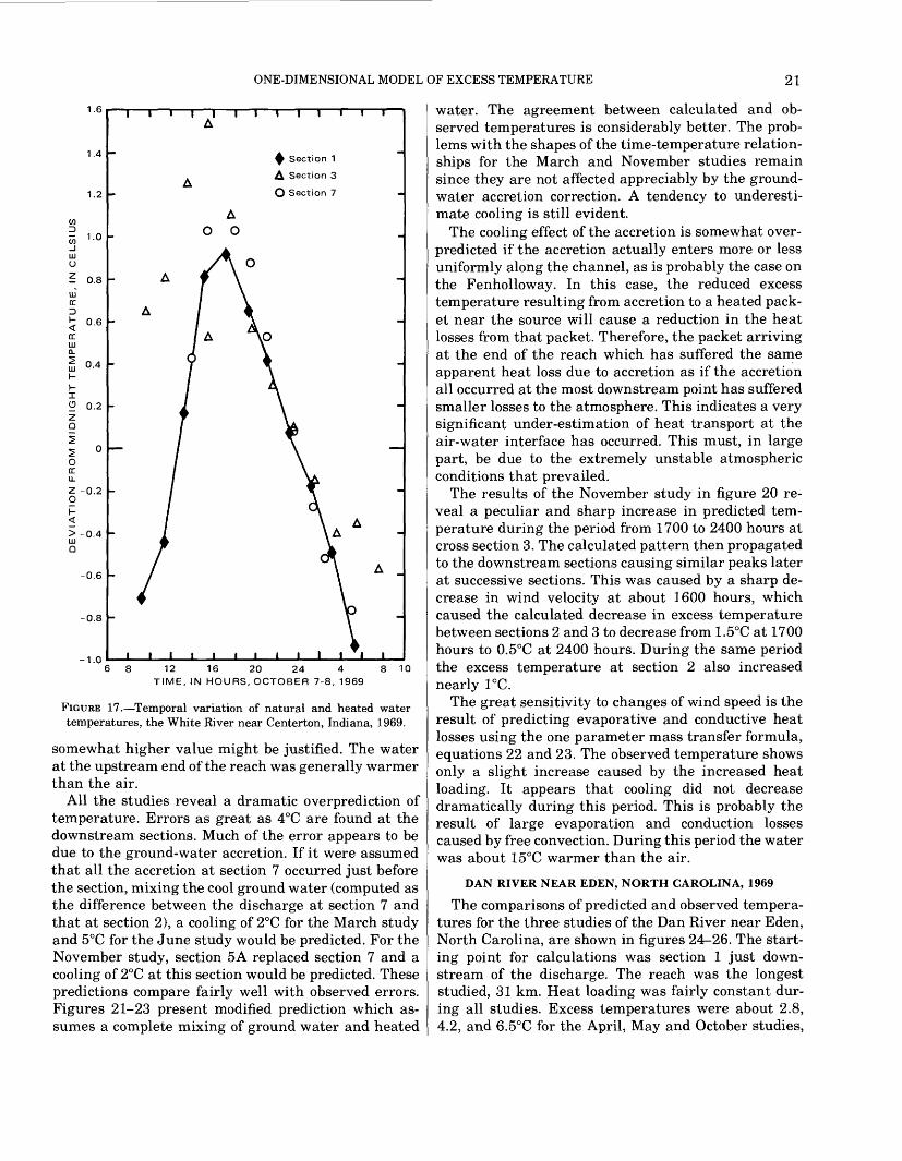
ONE-DIMENSIONAL MODEL OF EXCESS TEMPERATURE 21
1.6
1.4
1.2
m U
? 0.8
0.6
0.4IllI-I-1C? 0.22O
2 -0.2O
> -0.4m O
-0.6
-0.8
1.0
^ Section 1
A Section 3
O Section 7
12 16 20 24 4TIME, IN HOURS, OCTOBER 7-8, 1969
8 10
FIGURE 17. Temporal variation of natural and heated water temperatures, the White River near Centerton, Indiana, 1969.
somewhat higher value might be justified. The water at the upstream end of the reach was generally warmer than the air.
All the studies reveal a dramatic overprediction of temperature. Errors as great as 4°C are found at the downstream sections. Much of the error appears to be due to the ground-water accretion. If it were assumed that all the accretion at section 7 occurred just before the section, mixing the cool ground water (computed as the difference between the discharge at section 7 and that at section 2), a cooling of 2°C for the March study and 5°C for the June study would be predicted. For the November study, section 5A replaced section 7 and a cooling of 2°C at this section would be predicted. These predictions compare fairly well with observed errors. Figures 21-23 present modified prediction which as sumes a complete mixing of ground water and heated
water. The agreement between calculated and ob served temperatures is considerably better. The prob lems with the shapes of the time-temperature relation ships for the March and November studies remain since they are not affected appreciably by the ground- water accretion correction. A tendency to underesti mate cooling is still evident.
The cooling effect of the accretion is somewhat over- predicted if the accretion actually enters more or less uniformly along the channel, as is probably the case on the Fenholloway. In this case, the reduced excess temperature resulting from accretion to a heated pack et near the source will cause a reduction in the heat losses from that packet. Therefore, the packet arriving at the end of the reach which has suffered the same apparent heat loss due to accretion as if the accretion all occurred at the most downstream point has suffered smaller losses to the atmosphere. This indicates a very significant under-estimation of heat transport at the air-water interface has occurred. This must, in large part, be due to the extremely unstable atmospheric conditions that prevailed.
The results of the November study in figure 20 re veal a peculiar and sharp increase in predicted tem perature during the period from 1700 to 2400 hours at cross section 3. The calculated pattern then propagated to the downstream sections causing similar peaks later at successive sections. This was caused by a sharp de crease in wind velocity at about 1600 hours, which caused the calculated decrease in excess temperature between sections 2 and 3 to decrease from 1.5°C at 1700 hours to 0.5°C at 2400 hours. During the same period the excess temperature at section 2 also increased nearly 1°C.
The great sensitivity to changes of wind speed is the result of predicting evaporative and conductive heat losses using the one parameter mass transfer formula, equations 22 and 23. The observed temperature shows only a slight increase caused by the increased heat loading. It appears that cooling did not decrease dramatically during this period. This is probably the result of large evaporation and conduction losses caused by free convection. During this period the water was about 15°C warmer than the air.
DAN RIVER NEAR EDEN, NORTH CAROLINA, 1969
The comparisons of predicted and observed tempera tures for the three studies of the Dan River near Eden, North Carolina, are shown in figures 24-26. The start ing point for calculations was section 1 just down stream of the discharge. The reach was the longest studied, 31 km. Heat loading was fairly constant dur ing all studies. Excess temperatures were about 2.8, 4.2, and 6.5°C for the April, May and October studies,
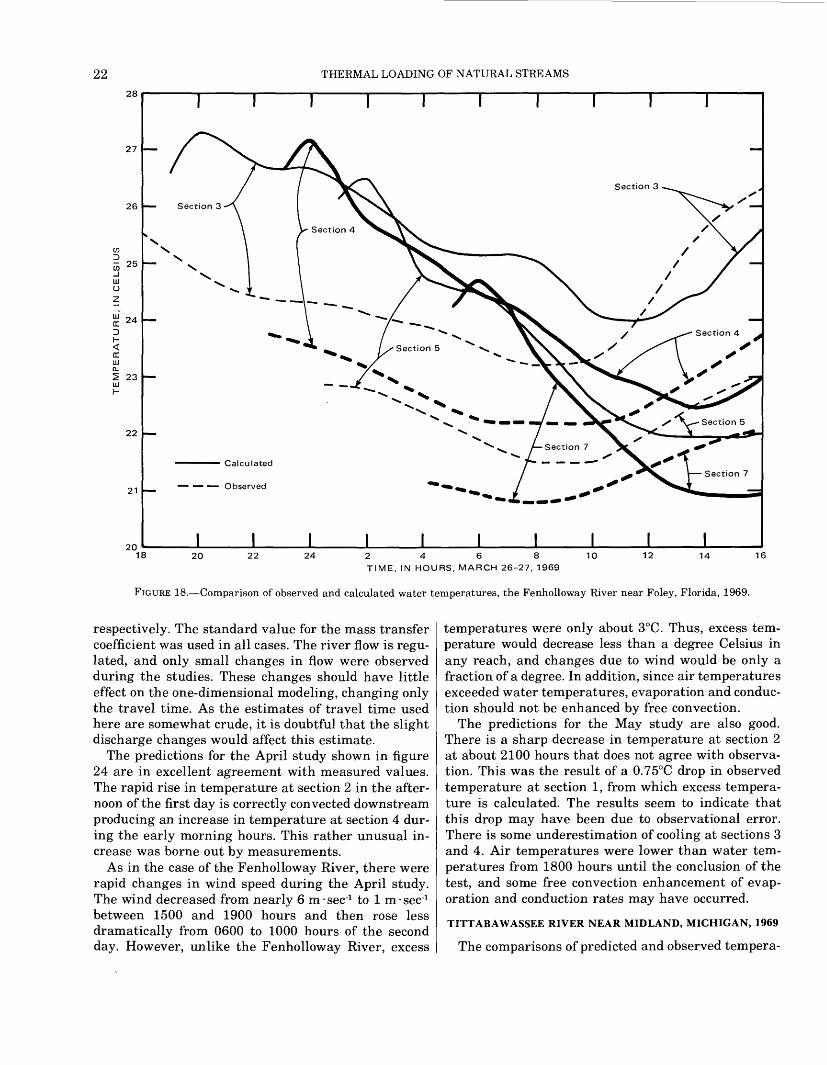
22 THERMAL LOADING OF NATURAL STREAMS
2468
TIME, IN HOURS, MARCH 26-27, 1969
FIGURE 18. Comparison of observed and calculated water temperatures, the Fenholloway River near Foley, Florida, 1969.
respectively. The standard value for the mass transfer coefficient was used in all cases. The river flow is regu lated, and only small changes in flow were observed during the studies. These changes should have little effect on the one-dimensional modeling, changing only the travel time. As the estimates of travel time used here are somewhat crude, it is doubtful that the slight discharge changes would affect this estimate.
The predictions for the April study shown in figure 24 are in excellent agreement with measured values. The rapid rise in temperature at section 2 in the after noon of the first day is correctly convected downstream producing an increase in temperature at section 4 dur ing the early morning hours. This rather unusual in crease was borne out by measurements.
As in the case of the Fenholloway River, there were rapid changes in wind speed during the April study. The wind decreased from nearly 6 m sec'1 to 1 m sec'1 between 1500 and 1900 hours and then rose less dramatically from 0600 to 1000 hours of the second day. However, unlike the Fenholloway River, excess
temperatures were only about 3°C. Thus, excess tem perature would decrease less than a degree Celsius in any reach, and changes due to wind would be only a fraction of a degree. In addition, since air temperatures exceeded water temperatures, evaporation and conduc tion should not be enhanced by free convection.
The predictions for the May study are also good. There is a sharp decrease in temperature at section 2 at about 2100 hours that does not agree with observa tion. This was the result of a 0.75°C drop in observed temperature at section 1, from which excess tempera ture is calculated. The results seem to indicate that this drop may have been due to observational error. There is some underestimation of cooling at sections 3 and 4. Air temperatures were lower than water tem peratures from 1800 hours until the conclusion of the test, and some free convection enhancement of evap oration and conduction rates may have occurred.
TITTABAWASSEE RIVER NEAR MIDLAND, MICHIGAN, 1969
The comparisons of predicted and observed tempera-
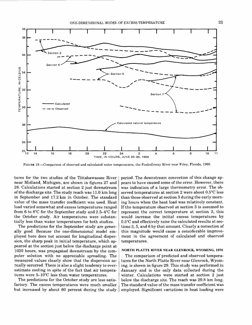
ONE-DIMENSIONAL MODEL OF EXCESS TEMPERATURE 23
39
38
36
32
30
28
26
25
Section 4
Calculated
Observed
Calculated natural temperature
13 14 16 18 20 22 24 2TIME, IN HOURS, JUNE 25-26, 1969
10 11
FIGURE 19. Comparison of observed and calculated water temperatures, the Fenholloway River near Foley, Florida, 1969.
tures for the two studies of the Tittabawassee River near Midland, Michigan, are shown in figures 27 and 28. Calculations started at section 2 just downstream of the discharge site. The study reach was 11.0 km long in September and 17.2 km in October. The standard value of the mass transfer coefficient was used. Heat load varied somewhat and excess temperatures ranged from 6 to 8°C for the September study and 2.5-4°C for the October study. Air temperatures were substan tially less than water temperatures for both studies.
The predictions for the September study are gener ally good. Because the one-dimensional model em ployed here does not account for longitudinal disper sion, the sharp peak in initial temperature, which ap peared at the section just below the discharge point at 1030 hours, was propagated downstream by the com puter solution with no appreciable spreading. The measured values clearly show that the dispersion ac tually occurred. There is also a slight tendency to over estimate cooling in spite of the fact that air tempera tures were 5-10°C less than water temperatures.
The predictions for the October study are less satis factory. The excess temperatures were much smaller but increased by about 60 percent during the study
period. The downstream convection of this change ap pears to have caused some of the error. However, there was indication of a large thermometry error. The ob served temperatures at section 2 were about 0.5°C less than those observed at section 3 during the early morn ing hours when the heat load was relatively constant. If the temperature observed at section 3 is assumed to represent the correct temperature at section 2, this would increase the initial excess temperatures by 0.5°C and effectively raise the calculated results at sec tions 3, 5, and 6 by that amount. Clearly a correction of this magnitude would cause a considerable improve ment in the agreement of calculated and observed temperatures.
NORTH PLATTE RIVER NEAR GLENROCK, WYOMING, 1970
The comparison of predicted and observed tempera tures for the North Platte River near Glenrock, Wyom ing, is shown in figure 29. This study was performed in January and is the only data collected during the winter. Calculations were started at section 2 just below the discharge site. The reach was 29.8 km long. The standard value of the mass transfer coefficient was employed. Significant variations in heat loading were
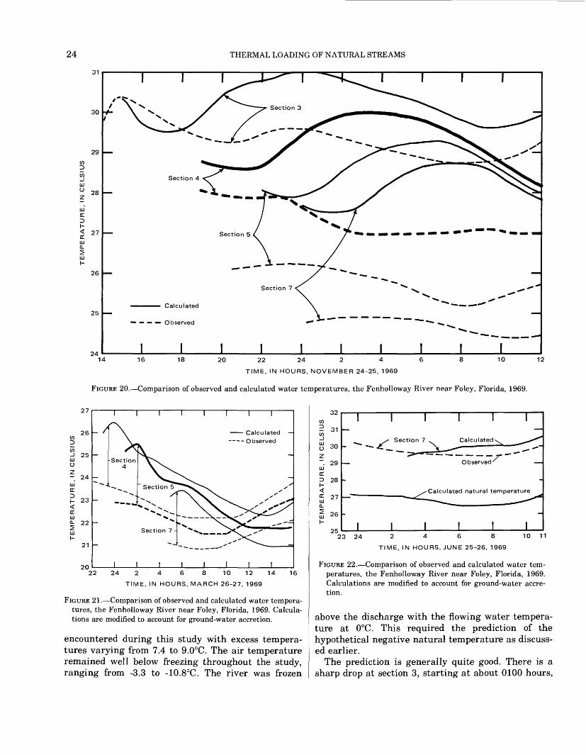
24 THERMAL LOADING OF NATURAL STREAMS
31
30
29
28
< 27
UJ
26
25
24
Se
Section
^^^ Calculated
Observed
14 16 18 20 22 24 2 4
TIME, IN HOURS, NOVEMBER 24-25, 1969
10 12
FIGURE 20. Comparison of observed and calculated water temperatures, the Fenholloway River near Foley, Florida, 1969.
27
26
25UJo
- 24UJ DC
H 23
DC UJ o. 22
UJ H
21
20
I I
Calculated -- Observed
Section 7 -
22 24 2 4 6 8 10 12 14
TIME, IN HOURS, MARCH 26-27, 1969
16
FIGURE 21. Comparison of observed and calculated water tempera tures, the Fenholloway River near Foley, Florida, 1969. Calcula tions are modified to account for ground-water accretion.
encountered during this study with excess tempera tures varying from 7.4 to 9.0°C. The air temperature remained well below freezing throughout the study, ranging from -3.3 to -10.8°C. The river was frozen
J^w2 31w_iUJo 30z~ 29UJDCD 28H<DC 27UJQ.
U 26H
OK
I I I I I I
__ .
,^ ^ Section 7 ^ Calculated^ ^^-^x***
"^ _ ^ -*^" l^^- <**
_ Observed^
.
__ ^Calculated natural temperature
~^~^.^^ ^ -""'^
.
I I I I I I
23 24 2 4 6 8
TIME, IN HOURS, JUNE 25-26, 1969
10 11
FIGURE 22. Comparison of observed and calculated water tem peratures, the Fenholloway River near Foley, Florida, 1969. Calculations are modified to account for ground-water accre tion.
above the discharge with the flowing water tempera ture at 0°C. This required the prediction of the hypothetical negative natural temperature as discuss ed earlier.
The prediction is generally quite good. There is a sharp drop at section 3, starting at about 0100 hours,
30
29
U 28
m 0-7IT 27D H < IT 26LU
25
24
ONE-DIMENSIONAL MODEL OF EXCESS TEMPERATURE
27
25
Section
Section 5A
Calculated ~"
Observed
I I I
19 20 22 24 2 4 6 8 10
TIME, IN HOURS, NOVEMBER 24-25, 1969
12
FIGURE 23. Comparison of observed and calculated water temper atures, the Fenholloway River near Foley, Florida, 1969. Calcu lations are modified to account for ground-water accretion.
17.2
. 17
16
15
14.6
I I I T
Calculated--- Observed
I I I
Section 4
I I I I I1314 16 18 20 22 24 2 4 6 8 1011
TIME, IN HOURS, APRIL 2-3, 1969
FIGURE 24. Comparison of observed and calculated water tempera tures, the Dan River near Eden, North Carolina, 1969.
which does not appear in the data. This was induced in the solution by a drop of 0.8°C in the excess tempera ture at the starting point, section 2, occuring between 2400 and 0200 hours. It is possible that the tempera ture measurement at 0200 hours, which was consider ably lower than that at 2400 hours and that at 0355 hours, may have resulted from temporary input condi tions and was not representative of the temperature at section 2 from 0100 to 0300 hours. The prediction would surely have been better had the temperature at 0200 hours at section 2 been 0.5°C higher. There was also an increase in wind speed from 2 m-sec 1 to 4 m-sec-1 that occurred at about 0100 hours and caused a sharp reduction in the value of Te at section 3.
There is some overestimation of cooling, particularly during the early morning hours. During this period, ice formation occurred at the right bank (discharge was
D 26
25
24
23
I I T
Calculated
Observed
Section 2
I I
12 14 16 18 20 22 24 2 4 6 8 10
TIME, IN HOURS, MAY 6-7, 1969
FIGURE 25. Comparison of observed and calculated water temper atures, the Dan River near Eden, North Carolina, 1969.
28
27
UJ 26 DCD I-
25
24
I I I I I I I I I
24 2 4 6 8 10 12 14 16 18 20 22
TIME, IN HOURS, SEPTEMBER 16-17, 1969
24
FIGURE 26. Comparison of observed and calculated water tempera tures, the Dan River near Eden, North Carolina, 1969.
concentrated on the left bank). This condition ceased somewhere between sections 3 and 4 where mixing supplied enough heat at the right bank to prevent ice formation. There is no quantitative information on the amount of ice that formed. However, any ice formation has the effect of liberating heat to the remainder of the system and would cause observed temperatures to be higher than expected. The melting of ice, which was complete by 1100 hours, would require energy from the rest of the system. This would lower the temperature or, more precisely, slow the rate of increase of tempera-
26 THERMAL LOADING OF NATURAL STREAMS
25
24
23
22
21
Section 3
Calculated--- Observed
I I I
8 10 12 14 16 18 20 22 24 2 4 6
TIME, IN HOURS,SEPTEMBER 18-19, 1969
FIGURE 27. Comparison of observed and calculated water temper atures, the Tittabawassee River near Midland, Michigan, 1969.
11
W0 10
i i iiii i i i i r
Section 5
Section 3
Calculated--- Observed
16 18 20 22 24 2 4 6 8 10 12 14
TIME, IN HOURS, OCTOBER 28-29, 1969
FIGURE 28. Comparison of observed and calculated water tempera tures, the Tittabawasee River near Midland, Michigan, 1969.
4.5
LII ccDH< 2ocLU
0.5
I I T
Calculated ~ --- Observed
I___I J___I18 20 22 24 2 4 6 8 10 12 14 16
TIME, IN HOURS, JANUARY 28-29, 1970
FIGURE 29. Comparison of observed and calculated water tempera tures, the North Platte River near Glenrock, Wyoming, 1970.
ture in the postdawn hours, and thereafter prediction and observation should agree. Excepting this ice for mation, the estimate of cooling appears to have been quite good.
WEST BRANCH OF THE SUSQUEHANNA RIVER
NEAR SHAWVILLE, PENNSYLVANIA, 1962
The comparison of predicted and observed tempera tures for the West Branch of the Susquehanna River near Shawville, Pennsylvania, is shown in figure 30. Calculations were started at section 0 just below the discharge site. The total reach length was 24.1 km. The standard value for the mass transfer coefficient was used. Excess temperatures were quite high, ranging from 12 to 13.5°C at section 0. Air temperatures were less than water temperatures at all times.
The prediction is generally quite good and, in par ticular, the average dissipation seems to have been es timated quite well. Nevertheless, because of the high excess temperature, a problem similar to that encoun tered during the November study on the Fenholloway River can be noted. A sharp decrease in wind speed at about 1800 hours resulted in such a great rate of in crease in the excess temperature that the predicted total temperature started rising in spite of decreasing natural temperature. After the low windspeed had per sisted for a period equal to a travel time, all the heated water packets arriving at section 1 had experienced only low windspeeds and excess temperature stabiliz ed, and the total temperature decreased owing to de creasing natural temperature.
Unlike the November study on the Fenholloway River, there is no appearance that evaporation and conduction have been underestimated using standard mass transfer expressions. In light of the highly unsta ble conditions that existed, this is difficult to understand.
CONCLUSIONS REGARDING ONE-DIMENSIONAL MODELING
For most of the sites studied, the one-dimensional, nondispersive Lagrangian model would appear to be adequate for downstream temperature prediction. Rapid changes in heat loading rates may induce lon gitudinal temperature gradients so sharp that disper sion must be considered. This is evident in the results for the September study on the Tittabawassee River.
In most cases the conventional mass transfer formu lation of equation 14 appears adequate using a mass transfer coefficient of 2.68- 10* kg-nv1 - newton-1 . In the case of the Fenholloway River, this value is appar ently too small. This is not entirely surprising in light of the area dependence of the mass transfer coefficient as given by equation 15 and the fact that the Fenhol-
TWO-DIMENSIONAL MODEL OF EXCESS TEMPERATURE 27
Observed natural temperature
10 12 14 16 18 20 22 24 2 4 6
TIME, IN HOURS, OCTOBER 17-18, 1962
FIGURE 30. Comparison of observed and calculated water tempera tures, west branch of the Susquehanna River near Shawville, Pennsylvania, 1962.
loway River was by far the smallest stream studied. It would also appear that the predicted mass transfer is too sensitive to changes in wind velocity where unsta ble atmospheric conditions prevail. This is particularly evident in the results from the Fenholloway River and the West Branch of the Susquehanna River, where very large excess temperatures made the sensitivity of heat exchange to changes in wind velocity obvious.
The calculations strongly support the conclusion, evident from a consideration of the data, that very long reaches are required to dissipate the majority of the waste heat added to a stream. This is particularly true if the excess temperature at the point of discharge is low a requirement now imposed by most states on waste heat discharges. Only in the cases of the Fenhol loway River and the West Branch of the Susquehanna River were heat losses at the end of the study reach greater than 50 percent of the heat added. In both cases the excess temperatures were far above those now permitted by most states.
The above conclusion suggests that calculations such as proposed here may be necessary in the operation and siting of power plants downstream of existing waste heat sources. If regulations are designed to per mit excess temperature no greater than some specified figure, a downstream facility should not be permitted that full figure if an upstream discharge exists. But since neither the natural nor the excess temperature can be measured immediately above the downstream facility, either the natural temperature or the excess temperature at that point will require calculation. If the stream thermal regime is reasonably homogene ous, the excess temperature is the clear choice.
TWO-DIMENSIONAL MODEL OF EXCESS TEMPERATURE
MODEL FOR A STEADY UNIFORM CHANNEL
The two-dimensional equation for thermal balance in a natural water body was derived previously as equation 4. In order to develop a working model for natural streams, it must be simplified as for the one- dimensional models. The source-sink term, S, and the bottom heat exchange term, H^, are neglected. The flow is assumed to be steady uniform so that the depth-averaged transverse velocity, vz , is nonexistent and Y and vx are sole functions of z. The longitudinal dispersion term will be neglected on the grounds dis cussed previously. All these assumptions reduce equa tion 4 to
dT I ddt
dT H (42)
In equation 42, T is the depth-averaged water tem perature, vx the depth-averaged longitudinal velocity, and Kz is the depth-averaged thermal dispersion coeffi cient. The symbol H is the surface heat influx and Y is the depth.
Following the same approach as in the one-dimen sional model, the excess temperature Te is defined as (T-Tn \ where Tn is the temperature that would occur under the same meteorologic and hydraulic conditions if there was no waste heat discharge. The surface influx will be linearized by means of equations 24, 25, and 26. The resulting equation for Te is
dt+v x dx dz
(43) l '
Equation 43 forms a boundary value problem in a steady uniform flow when combined with proper boundary conditions. Because of the dependence of vx, Y, and Kz on z, however, a closed form solution is not obtainable for equation 43, and it must be solved nu merically.
A simpler approach to equation 43 is possible if the boundary condition is simplified such that waste wa ter discharge and excess temperature are assumed to be steady at the discharge site. It consists of combining the one-dimensional exponential decay model for sur face heat dissipation with the two-dimensional steady-state diffusion model developed by Yotsukura and Cobb (1972). Notice that if the excess heat were conservative so that U* =0, equation 43 is reduced to a steady-state equation
(44)dx dz
28 THERMAL LOADING OF NATURAL STREAMS
Suppose that T'e , the hypothetical excess temperature without decay, satisfies equation 44. Because the heat decay due to surface dissipation is a slow process rela tive to the heat transport by convection and diffusion, its parameter UJY may be approximated by Uj{Y}, which is a function of time alone if JF}, the cross- sectional average depth, is constant. Accordingly a so lution to equation 43 is proposed as
Te (x,z,t)=T'e (x,z)exp (- f' - (45)
Equation 45 can be shown to satisfy equation 43 if the heat decay term is replaced by UX TJ\Y} in equation 43.
Even though equation 45 is derived conceptually from the form of product solutions frequently used in the diffusion of reacting solutes (Crank, 1967), it could also be viewed as a combination of an Eulerian solu tion to diffusion and a Lagrangian solution to dissipa tion. It is similar to the approach used by Yeh, Verma, and Lai (1973) in the prediction of excess temperature for a cooling pond. Equation 45 should be considered as an approximation to what is physically going on rather than as a rigorous solution to a boundary value prob lem. The decay term in equation 45 will be calculated in terms of travel time in the same Lagrangian sense as in the one-dimensional model.
As for steady-state solutions to equation 44, the ap proach used by Yotsukura and Cobb (1972) consists of transforming equation 44 into
(46)dx ~ dq dq
where q is the partial cumulative discharge measured from one side of a cross section and is defined by
q=fvx Ydz'.T J o X .
(47)
Note that q=Q when the integration in equation 47 is carried over the entire cross section. Equation 46, in which q replaces z as the independent variable, is sim pler to handle than equation 44, because the convec- tive velocity is reduced to unity. The new coefficient in the dispersive term of equation 46, KzvxY2, may be ap proximated by a constant cross-sectional average value, {KzvxY2 }, so that the following approximate so lution is given to equation 46:
T'e (a,q')=-Teo erf
~erfV2
+ 2 erf V2
a(q'sl -2n+djq') erf V2~ (48)
The symbol Teo is the steady excess temperature at the initial cross section, where Qs is the steady excess water discharge rate and pCpQsTeo represents an inflow rate of excess heat. Summation with respect to index j is defined by 81 = + 1 and 62 = !. The symbol a is a nondimensional longitudinal distance parameter,
a=VQ 2/2x{KzvxY2 } , (49)
while q', fractional cumulative discharge q/Q, repre sents a transverse position. The symbols q' sl and q' s2 are fractions qsl/Q and qs2/Q respectively, where qal and qs2 represent the two ends of a part of streamflow con taminated by excess temperature at the initial section andqs2 -qsl =Qs .
By means of field tracer tests Yotsukura and Cobb (1972) showed that equation 48 is quite satisfactory for a number of straight uniform channels and is also usa ble in a moderately meandering reach of the Missouri River.
MODEL FOR A STEADY NATURAL STREAM
In applying equation 45 to a steady natural stream, it is necessary to subdivide a study reach into a set of steady uniform channels. A river system is visualized first as a flow system consisting of a fixed number of stream tubes with equal subdischarge Ag. This is shown in figure 31. Note that all solid lines represent impervious boundaries through which no convection and diffusion take place. The system is then divided into a set of subreaches depending on the uniformity of cross-sectional properties. A subreach may further be divided into subchannels depending on the location of tributaries and islands as illustrated in figure 31. In the stream-tube flow system longitudinal distance re mains the same as in the real river system.
Solutions to "conservative" excess temperature, T'e , are obtained for successive downstream subreaches starting at the waste heat discharge site. For each un iform subchannel, an upstream T'e is treated as the initial temperature, Teo , and downstream T'e is calcu lated by means of equation 48. In most applications, the upstream temperature tends to be different from one stream tube to another so that a superposition of solutions is required to obtain the downstream T'e re sulting from all upstream temperatures. This proce dure is justified because all differential equations in volved are linear equations.
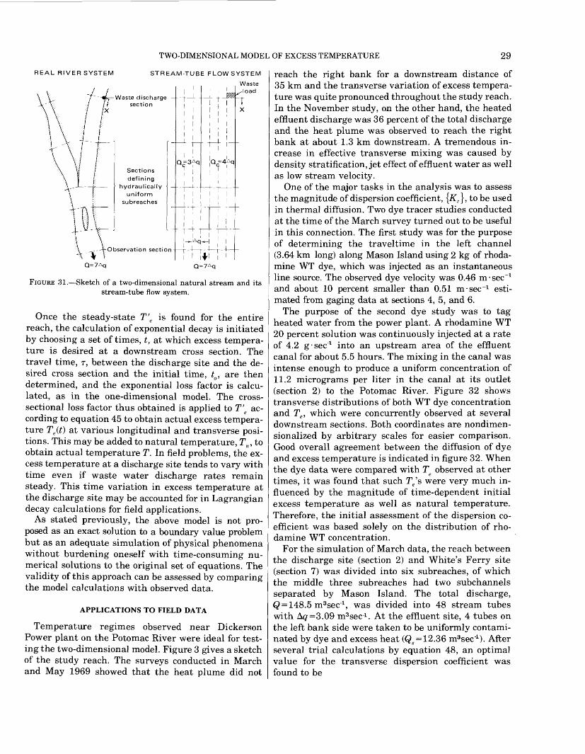
TWO-DIMENSIONAL MODEL OF EXCESS TEMPERATURE 29
REAL RIVER SYSTEM STREAM-TUBE FLOW SYSTEM
Waste /load
7X
Waste discharge - ---) -
section
Sectionsdefining
hydraulicallyuniform
subreaches
Observation section
Q=4Aq
FIGURE 31. Sketch of a two-dimensional natural stream and its stream-tube flow system.
Once the steady-state T'e is found for the entire reach, the calculation of exponential decay is initiated by choosing a set of times, t, at which excess tempera ture is desired at a downstream cross section. The travel time, T, between the discharge site and the de sired cross section and the initial time, t0 , are then determined, and the exponential loss factor is calcu lated, as in the one-dimensional model. The cross- sectional loss factor thus obtained is applied to T'e ac cording to equation 45 to obtain actual excess tempera ture Te (t) at various longitudinal and transverse posi tions. This may be added to natural temperature, Tn , to obtain actual temperature T. In field problems, the ex cess temperature at a discharge site tends to vary with time even if waste water discharge rates remain steady. This time variation in excess temperature at the discharge site may be accounted for in Lagrangian decay calculations for field applications.
As stated previously, the above model is not pro posed as an exact solution to a boundary value problem but as an adequate simulation of physical phenomena without burdening oneself with time-consuming nu merical solutions to the original set of equations. The validity of this approach can be assessed by comparing the model calculations with observed data.
APPLICATIONS TO FIELD DATA
Temperature regimes observed near Dickerson Power plant on the Potomac River were ideal for test ing the two-dimensional model. Figure 3 gives a sketch of the study reach. The surveys conducted in March and May 1969 showed that the heat plume did not
reach the right bank for a downstream distance of 35 km and the transverse variation of excess tempera ture was quite pronounced throughout the study reach. In the November study, on the other hand, the heated effluent discharge was 36 percent of the total discharge and the heat plume was observed to reach the right bank at about 1.3 km downstream. A tremendous in crease in effective transverse mixing was caused by density stratification, jet effect of effluent water as well as low stream velocity.
One of the major tasks in the analysis was to assess the magnitude of dispersion coefficient, {K,}, to be used in thermal diffusion. Two dye tracer studies conducted at the time of the March survey turned out to be useful in this connection. The first study was for the purpose of determining the traveltime in the left channel (3.64 km long) along Mason Island using 2 kg of rhoda- mine WT dye, which was injected as an instantaneous line source. The observed dye velocity was 0.46 m-sec"1 and about 10 percent smaller than 0.51 m-sec"1 esti mated from gaging data at sections 4, 5, and 6.
The purpose of the second dye study was to tag heated water from the power plant. A rhodamine WT 20 percent solution was continuously injected at a rate of 4.2 g-sec"1 into an upstream area of the effluent canal for about 5.5 hours. The mixing in the canal was intense enough to produce a uniform concentration of 11.2 micrograms per liter in the canal at its outlet (section 2) to the Potomac River. Figure 32 shows transverse distributions of both WT dye concentration and Te , which were concurrently observed at several downstream sections. Both coordinates are nondimen- sionalized by arbitrary scales for easier comparison. Good overall agreement between the diffusion of dye and excess temperature is indicated in figure 32. When the dye data were compared with Tg observed at other times, it was found that such Te 's were very much in fluenced by the magnitude of time-dependent initial excess temperature as well as natural temperature. Therefore, the initial assessment of the dispersion co efficient was based solely on the distribution of rho damine WT concentration.
For the simulation of March data, the reach between the discharge site (section 2) and White's Ferry site (section 7) was divided into six subreaches, of which the middle three subreaches had two subchannels separated by Mason Island. The total discharge, Q = 148.5 m3 sec~1 , was divided into 48 stream tubes with Ag=3.09 m3sec-1 . At the effluent site, 4 tubes on the left bank side were taken to be uniformly contami nated by dye and excess heat (Qs = 12.36 m3 sec"1 ). After several trial calculations by equation 48, an optimal value for the transverse dispersion coefficient was found to be
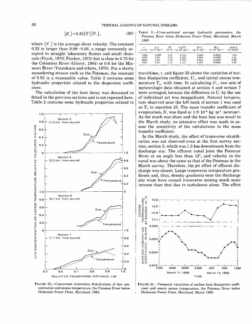
30 THERMAL LOADING OF NATURAL STREAMS
(50)
where {V*} is the average shear velocity. The constant 0.52 is larger than 0.08 0.26, a range commonly ac cepted in straight laboratory flumes and small chan nels (Prych, 1970; Fischer, 1973) but is close to 0.72 for the Columbia River (Glover, 1964) or 0.6 for the Mis souri River (Yotsukura and others, 1970). For a slowly meandering stream such as the Potomac, the constant of 0.52 is a reasonable value. Table 2 contains some hydraulic properties related to the dispersion coeffi cient.
The calculation of the heat decay was discussed in detail in the previous sections and is not repeated here. Table 2 contains some hydraulic properties related to
1.0
o.s
0.6
0.4
0.2
o
Section 3 (1.3 km from source)
1.0
0.8
0.6
0.4
0.2
0
/ Temperature
Section 6 (6.1 km from source)
Dye
Temperature
Section 7 (7.7 km from source)
1.0
0.8
0.6
0.4
0.2
0
0.5 0.6 0.7 0.8 0.9 1
RELATIVE TRANSVERSE DISTANCE,z/W
1.0
0.8
0.6
0.4
0.2
FIGURE 32. Concurrent transverse distributions of dye con centration and excess temperature, the Potomac River below Dickerson Power Plant, Maryland, 1969.
TABLE 2. Cross-sectional average hydraulic parameters, the Potomac River below Dickerson Power Plant, Maryland, March 1969
X t'.rl(in m) (in m-sec"1 1
2424519760617637
0.3650.580.290.30
[Y] [( , y«
(in m) (in m3 -sec"1 )
1.070.731.341.74
0.7240.3450.7651.127
[V*](in m sec"1 )
0.0400.0330.0440.051
[KZ](in m2 sec"1 )
0.02230.01250.03040.0458
Ax/[i'jr](in hours)
1.841.330.831.46
traveltime, T, and figure 33 shows the variation of sur face dissipation coefficient, £7*, and initial excess tem perature Teo with time. In calculating £/*, two sets of meteorologic data obtained at section 4 and section 7 were averaged, because the difference in £7* by the use of individual set was insignificant. Natural tempera ture observed near the left bank of section 1 was used as Tb in equation 25. The mass transfer coefficient of evaporation, N, was fixed at 1.9-1Q-8 kg-nr1 -newton-1 . As the reach was short and the heat loss was small in the March study, no intensive effort was made to as sess the sensitivity of the calculations to the mass transfer coefficient.
In the March study, the effect of transverse stratifi cation was not observed even at the first survey sec tion, section 3, which was 1.3 km downstream from the discharge site. The effluent canal joins the Potomac River at an angle less than 12°, and velocity in the canal was about the same as that of the Potomac in the March survey. Therefore, the jet effect of effluent dis charge was absent. Large transverse temperature gra dients and, thus, density gradients near the discharge site must have caused transverse mixing much more intense than that due to turbulence alone. The effect
1200 1600 2000 2400 400 800 1200
March 11, 1969 March 12, 1969
TIME
FIGURE 33. Temporal variations of surface heat dissipation coeffi cient and source excess temperature, the Potomac River below Dickerson Power Plant, Maryland, March 1969.
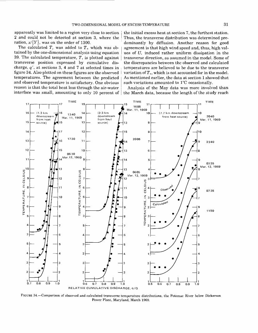
TWO-DIMENSIONAL MODEL OF EXCESS TEMPERATURE 31
apparently was limited to a region very close to section 2 and could not be detected at section 3, where the ration, Jt/JY}, was on the order of 1300.
The calculated Te was added to Tn which was ob tained by the one-dimensional analysis using equation 39. The calculated temperature, T, is plotted against transverse position expressed by cumulative dis charge, q', at sections 3, 4 and 7 at selected times in figure 34. Also plotted on these figures are the observed temperatures. The agreement between the predicted and observed temperature is satisfactory. One obvious reason is that the total heat loss through the air-water interface was small, amounting to only 10 percent of
the initial excess heat at section 7, the furthest station. Thus, the transverse distribution was determined pre dominantly by diffusion. Another reason for good agreement is that high wind speed and, thus, high val ues of t/* induced rather uniform dissipation in the transverse direction, as assumed in the model. Some of the discrepancies between the observed and calculated temperatures are believed to be due to the transverse variation of Tn , which is not accounted for in the model. As mentioned earlier, the data at section 1 showed that such variations amounted to 1°C occasionally.
Analysis of the May data was more involved than the March data, because the length of the study reach
17
16
15
14
13
12
(1.3 km downstream from heat
source)
TIME 17 15
16 1340 14 Mar. 1 1, 1969
15 13
17
173016 11
15 10
0530Mar.12, 1969
14 9
0.7 0.8 0.9 1.0
TIME 15 11
1605Mar. 11, 1969
14 10
2005
0605 Mar. 12, 1969
(7.7 km downstream
from heat source)
11TIME
102040
Mar. 11, 1969
0325 Mar. 12, 1969
0735
0.6 0.7 0.8 0.9 1.0
RELATIVE CUMULATIVE DISCHARGE, q/Q
1150
0.5 0.6 0.7 0.8 0.9 1.0
FIGURE 34. Comparison of observed and calculated transverse temperature distributions, the Potomac River below DickersonPower Plant, Maryland, March 1969.
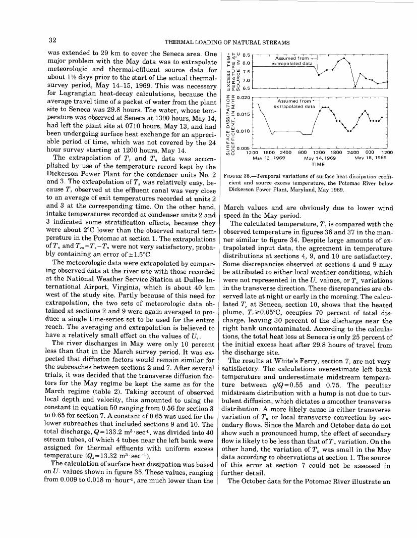
32 THERMAL LOADING OF NATURAL STREAMS
was extended to 29 km to cover the Seneca area. One major problem with the May data was to extrapolate meteorologic and thermal-effluent source data for about IVz days prior to the start of the actual thermal- survey period, May 14-15, 1969. This was necessary for Lagrangian heat-decay calculations, because the average travel time of a packet of water from the plant site to Seneca was 29.8 hours. The water, whose tem perature was observed at Seneca at 1300 hours, May 14, had left the plant site at 0710 hours, May 13, and had been undergoing surface heat exchange for an appreci able period of time, which was not covered by the 24 hour survey starting at 1200 hours, May 14.
The extrapolation of Ts and Tn data was accom plished by use of the temperature record kept by the Dickerson Power Plant for the condenser units No. 2 and 3. The extrapolation of Ts was relatively easy, be cause Ts observed at the effluent canal was very close to an average of exit temperatures recorded at units 2 and 3 at the corresponding time. On the other hand, intake temperatures recorded at condenser units 2 and 3 indicated some stratification effects, because they were about 2°C lower than the observed natural tem perature in the Potomac at section 1. The extrapolations of Tn and Teo =Ts -Tn were not very satisfactory, proba bly containing an error of ±1.5°C.
The meteorologic data were extrapolated by compar ing observed data at the river site with those recorded at the National Weather Service Station at Dulles In ternational Airport, Virginia, which is about 40 km west of the study site. Partly because of this need for extrapolation, the two sets of meteorologic data ob tained at sections 2 and 9 were again averaged to pro duce a single time-series set to be used for the entire reach. The averaging and extrapolation is believed to have a relatively small effect on the values of U..
The river discharges in May were only 10 percent less than that in the March survey period. It was ex pected that diffusion factors would remain similar for the subreaches between sections 2 and 7. After several trials, it was decided that the transverse diffusion fac tors for the May regime be kept the same as for the March regime (table 2). Taking account of observed local depth and velocity, this amounted to using the constant in equation 50 ranging from 0.56 for section 3 to 0.65 for section 7. A constant of 0.65 was used for the lower subreaches that included sections 9 and 10. The total discharge, Q = 133.2 m3 -sec-1 , was divided into 40 stream tubes, of which 4 tubes near the left bank were assigned for thermal effluents with uniform excess temperature (Qs = 13.32 m3 -sec -1 ).
The calculation of surface heat dissipation was based on U values shown in figure 35. These values, ranging from 0.009 to 0.018 m -hour1 , are much lower than the
u. u_* g 0.005wu 1200 1800 2400
May 13,1969600 1200 1800
May 14, 1969
TIME
2400 600 1200 May 15, 1969
FIGURE 35. Temporal variations of surface heat dissipation coeffi cient and source excess temperature, the Potomac River below Dickerson Power Plant, Maryland, May 1969.
March values and are obviously due to lower wind speed in the May period.
The calculated temperature, T, is compared with the observed temperature in figures 36 and 37 in the man ner similar to figure 34. Despite large amounts of ex trapolated input data, the agreement in temperature distributions at sections 4, 9, and 10 are satisfactory. Some discrepancies observed at sections 4 and 9 may be attributed to either local weather conditions, which were not represented in the U.x values, or Tn variations in the transverse direction. These discrepancies are ob served late at night or early in the morning. The calcu lated Te at Seneca, section 10, shows that the heated plume, Te 5»0.05°C, occupies 70 percent of total dis charge, leaving 30 percent of the discharge near the right bank uncontaminated. According to the calcula tions, the total heat loss at Seneca is only 25 percent of the initial excess heat after 29.8 hours of travel from the discharge site.
The results at White's Ferry, section 7, are not very satisfactory. The calculations overestimate left bank temperature and underestimate midstream tempera ture between <?/Q = 0.55 and 0.75. The peculiar midstream distribution with a hump is not due to tur bulent diffusion, which dictates a smoother transverse distribution. A more likely cause is either transverse variation of Tn or local transverse convection by sec ondary flows. Since the March and October data do not show such a pronounced hump, the effect of secondary flow is likely to be less than that of Tn variation. On the other hand, the variation of Tn was small in the May data according to observations at section 1. The source of this error at section 7 could not be assessed in further detail.
The October data for the Potomac River illustrate an
TWO-DIMENSIONAL MODEL OF EXCESS TEMPERATURE 33
26
25
24
23
22
21
20
19
18
(2.3 km downstream from heat
source)
TIME
25
20
19
21
20
19
18
20
19
18
20
19
1040
May 14, 1969
22
26 1800
25
24
262400
25
24
23
25
0600 24 May 15, 1969
23
25
24
23
22
21
20
19
1000
0.7 0.8 0.9 1.0
RELATIVE CUMULATIVE
DISCHARGE, q/Q
23
22
21
20
19
18
17
20
19
18
HI0 20
(7.7 km downstream from heat source)
TIME
1205
May 14, 1969
21
Observed
Calculated
19
21
20
19
18
20
19
18
20
19
18
17
24
22
24
23
22
24
23
22
21
1600
2000
2400
230415
May 15, 1969
22
21
23
22
21
20
19
18
0815
0.0 0.2 0.4 0.6 0.8
RELATIVE CUMULATIVE DISCHARGE, q/Q
1.0
FIGURE 36. Comparison of observed and calculated transverse temperature distributions, the Potomac River below DickersonPower plant, Maryland, May 1969.
interesting effect of jet and transverse density currents of heated effluents. The Potomac flow was much lower in October relative to those in March and May. The effluent discharge of 18 m3 -sec"1 was flowing into the
ambient Potomac discharge of 32 m3 -sec"1 . The ratio, QJQ, was 36 percent. Furthermore, the effluent veloc ity of 0.90 m-sec-1 was high in comparison to the am bient Potomac velocity of 0.2 m-sec4 . The combined
34 THERMAL LOADING OF NATURAL STREAMS
TIME
1104
20 May 14, 1969
1710
2105
21 0300
May 15, 1969
1055
21 (28.8 km downstreamfrom heat source)^--
______ -r-~r« * . * *
2310
May 14, 1969
I 210505
20 May 15, 1969
20
19
18
0910
0 0.2 0.4 0.6 0.8 1.0RELATIVE CUMULATIVE DISCHARGE q/Q
FIGURE 37. Comparison of observed and calculated transverse temperature distributions, the Potomac River below Dickerson Power Plant, Maryland, May 1969.
effect of jet and transverse convection due to density currents was observable at section 3, where the verti cal temperature difference of more than 0.5°C existed between 40 and 20 m from the right bank. The depth in this area was 1.4-2.2 m. The total heated plume width at section 3 was on the order of 200 m in contrast to the width of 70 m in the March study, and the right edge of the plume was characterized by a 20-m-wide band of vertical nonuniformity in temperature.
Even though the present model assumes that the depth-averaged transverse velocity, vz , is zero every where, some transverse convective effects due to sec ondary flows or density currents are accommodated in the equation in terms of effective dispersion coefficient, Kz . The model can not accommodate the convective ef fects of jets or very strong secondary currents. An effort was made to simulate the distribution at section 3 by increasing the diffusion factor until the calculation matches with the data. The best simulation is shown in figure 38. In this calculation, the constant of the dis persion coefficient, equation 50, was increased to 11.0
(1.3km downstream from heat source)
TIME
1505 15 Oct. 29, 1969
2105
0310 Oct. 30, 1969
1105
0.0 0.2 0.4 0.6 0.8 1.0RELATIVE CUMULATIVE DISCHARGE q/Q
FIGURE 38. Comparison of observed and calculated transverse temperature distributions, the Potomac River below Dickerson Power Plant, Maryland, October 1969.
from 0.52. On the other hand, a constant of 0.65 could be used in all other downstream sections as expected. The results of calculations for lower subreaches are shown in figures 39 and 40.
In the October study as in the May study, meteor- ologic and effluent temperature data were extrapolated by comparing the survey data with those recorded at Dickerson Power Plant and Dulles weather station. Because the travel time to a downstream section was much longer than that for the May study, being 11.2, 25.7, and 59.7 hours for sections 7, 9, and 10 respec tively, almost half of the calculations for section 7 and all calculations for section 9 used some parts of ex trapolated data. The calculation at section 10 was not tried. The heat dissipation coefficient, £/*, varied from 0.007 to 0.02 m-hour"1 . This range is rather similar to that of the May study, indicating the predominant ef fect of wind speed on £7*. The simulation results shown in figures 38, 39, and 40 show that the present model
(7.7 km downstream from heat source)
TWO-DIMENSIONAL MODEL OF EXCESS TEMPERATURE
TIME
1200
Oct. 29, 1969
1600
2005
0005
Oct. 30, 1969
0405
0805
1215
0.0 0.1 0.2 0.3 0.4 0.5 0.6 0.7 0.8 0.9 1.0
RELATIVE CUMULATIVE DISCHARGE q/Q
FIGURE 39. Comparison of observed and calculated transverse temperature distributions, the Potomac River below Dickerson Power Plant, Maryland, October 19
with more adequate weather data and with current knowledge on dispersion coefficient can predict heated plume configurations with acceptable accuracy.
As for the effects of transverse density currents, it is worth mentioning the results of flume study reported by Prych (1970). He studied the transverse diffusion of excess heat in a rectangular flume by releasing a verti cal line heat source at ambient velocity. It is reported that the total transverse variance, cra 2 , could be consid ered as a sum of crt 2 due to regular turbulence diffusiv- ity and crs 2 due to density currents. At a distance on the order of jc/{Y}=2{^} {Y}/ {Kz}, crs2 stopped increasing because of reduced density currents, and the increase of cra 2 thereafter was entirely due to crt2 .
The prototype distance x corresponding to Prych's criterion is on the order of 30-50 m for the October data and is much smaller than x = 1330 m at section 3. Be cause the heat source on the Potomac River was a block
35
TIME14 1245
13 Oct. 29, 1969
1635
2035
0040
Oct. 30, 1969
0440
0830
1025
0 0.2 0.4 0.6 0.8 1.0 RELATIVE CUMULATIVE DISCHARGE q/Q
FIGURE 40. Comparison observed and calculated transverse tem perature distributions, the Potomac River below Dickerson Power Plant, Maryland, October 1969.
source rather than the line source used in the Prych's study, the effect of density currents must have per sisted for a much longer distance than 30 or 50 m. Similar effects must have been existent in the March and May data but were not observed at section 3. The observed pattern of density effects appears to agree with Prych's laboratory study.
The two-dimensional model was also applied to the Dan River and the North Platte River data. In both rivers the transverse nonuniformity of excess tempera ture was significant only in one downstream subreach. Because the river alinement was quite sinuous in both rivers, the temperature distributions at other sub- reaches were all uniform in the transverse direction. The one-dimensional analysis of these subreaches was discussed previously. Figures 41 and 42 present the simulations for one subreach in the Dan River and the North Platte River, respectively. The heat decay in these calculations was insignificant because the sub- reach length was small. The observed temperature dis tribution at the first cross section was used as the ini tial distribution in the calculation, because the effluent discharge condition was not compatible with the
36
km downstream from heat source) _
THERMAL LOADING
TIME
1310
April 2, 1969
1709
2200
0040
17 April 3, 1969
0537
0812
1022
0 0.2 0.4 0.6 0.8 1.0
RELATIVE CUMULATIVE DISCHARGE, q/Q
FIGURE 41. Comparison of observed and calculated transverse temperature distributions, the Dan River near Eden, North Carolina, April 1969.
model. Because of these reasons, figures 41 and 42 are considered as verifying the diffusion aspect of the model. A constant of 0.65 in equation 50 was used for both simulations.
SUMMARY REGARDING TWO-DIMENSIONAL MODEL
Ideally, a two-dimensional model for excess temper ature should be combined with a two-dimensional model for natural temperature. The latter model was not developed in the present analysis, and thus some discrepancies between observed and calculated tem peratures could not be resolved for the assessment of the two-dimensional model. A typical example is the low temperature near the banks as observed in figure 40.
Nevertheless, the overall performance of the present model appears to confirm that the combination of the steady-state diffusion solution and the Lagrangian decay solution is a feasible approach. In this connec tion, it is worth noting that an attempt was made in the early stage of analysis to solve equation 43 directly by Eulerian numerical approximations. It was aban doned because the calculations were much more time consuming and inefficient in terms of solution ac-
OF NATURAL STREAMS
9
(3.1 km downstream from heat source)
TIME
1620 Jen. 28,1970
2225
0405 4 Jan. 29, 1970
0805
1215
0 0.2 0.4 0.6 0.8 1.0
RELATIVE CUMULATIVE DISCHARGE q/Q
FIGURE 42. Comparison of observed and calculated transverse temperature distributions, the North Platte River near Glen- rock, Wyoming, January 1970.
curacies than the above-discussed model.A substantial amount of data extrapolation was re
quired for the two-dimensional analysis. This was caused by the incompatibility between the data collec tion scheme and the model development as noted pre viously. If thermal data are collected for the purpose of applying the present Lagrangian model, it is clear that the reach length and the travel time should be of prime considerations in planning such a data collection scheme.
It is apparent that verification concerning the trans port phase is more positive than that for the decay phase. A comparison of the present findings with other studies shows that there is little doubt that the trans verse heat dispersion coefficient, Kz , in the absence of abrupt temperature changes, is of the same order of magnitude as the mass dispersion coefficient for neu trally buoyant solutes. Even though the formulation of
SUMMARY AND CONCLUSIONS 37
equation 42 assumes no depth-averaged transverse velocity, the weak convective effect due to secondary or density currents is accommodated in terms of disper sion coefficient, Kz . Furthermore, by means of empiri cal adjustment of Kz , some pronounced convective ef fects could also be simulated by the model as shown in figure 38.
The analysis of the surface-heat decay in the present section is rather limited, as it was evaluated only for the Potomac reach, where heat losses were not sig nificant at most cross sections. Comparing a total heat loss of 25 percent, calculated for the section at Seneca by the two-dimensional model, with an observed value of 35 percent of figure 11, the magnitudes of both the dissipation coefficient, £/*, and the mass-transfer coeffi cient for evaporation, N, used in the present section may have been too low. The decay aspect has been discussed more extensively in the section on the one- dimensional model of excess temperature.
SUMMARY AND CONCLUSIONS
As explained in the "Introduction," development of the present mathematical models was based on the recognition that earlier models, such as the energy- budget equation, the equilibrium temperature, and the steady-state exponential decay law, are not suitable in analyzing short-term phenomena in a flowing natural stream. In concluding the report, therefore, it is appro priate to summarize pertinent features of the present mathematical models.
In order to approach short-term water temperature problems in a thermally loaded stream, the excess temperature, Te , is defined as a difference between ac tual water temperature, T, and natural temperature, Tn , which would exist in the stream under the same hydraulic and meteorologic conditions but without heat discharges. One major feature of the present ap proach is to solve the heat conservation equation sepa rately for Te and Tn . Both temperatures are functions of time and space variables.
Starting from a three-dimensional equation for con servation of thermal energy in a turbulent flow, two- and one-dimensional equations for water temperature, T, are obtained by integrating the equation, first, with respect to depth and, second, with respect to surface width of a stream channel. Two assumptions involved are that the heat exchange between water and sur rounding media takes place at the interface without storage and that the introduction of dispersion coeffi cients is justified empirically. No formal assumptions are required as to the steadiness or uniformity of a flow as long as the gradient-type dispersion terms are ac ceptable approximations.
The equation for Te is obtained by subtracting the equation for Tn from that for T. Assuming that the entire heat exchange occurs at the air-water interface, the resulting equation is shown to be independent of incoming solar and atmospheric radiation fluxes, the measurement of which requires expensive instrumen tation. Three other essential heat fluxes, namely, back radiation, latent heat of evaporation, and conduction are dependent on transient meteorologic conditions and are nonlinear functions of water temperature. However, these fluxes can be linearized with respect to T, provided that an arbitrarily chosen base tempera ture of linearization, Tb , does not deviate excessively from both T and Tn . The surface heat dissipation coeffi cient, U, is simply the sum of the first derivatives of the three heat fluxes with respect to temperature evaluated at Tb . In this manner, the equation for Te is reduced to a linear equation.
The one-dimensional equation for Te may be further reduced to an ordinary differential equation by ne glecting the longitudinal dispersion term and adopting the Lagrangian approach, which employs mean travel- time as the only independent variable. If time-varying initial excess temperature and wind speed are given as inputs, the excess temperature can be solved as a func tion of traveltime. For the two-dimensional equation for Te , a steady-state Eulerian solution is obtained for a hypothetical "conservative" excess temperature, as suming that both stream and waste heat discharges remain steady. The actual excess temperature is ap proximated by multiplying the "conservative" excess temperature by the Lagrangian heat decay factor simi lar to the one-dimensional model.
Only a one-dimensional model is considered for natural temperature in this analysis. The incoming solar and atmospheric radiations are important input data. Linearization of the other three heat fluxes is not employed in the equation for Tn , because the nonlinear effect is small in the normal range of variation of Tn and these three fluxes at certain times are adequately approximated by use of the known temperature at an immediately preceding time. The solutions are ob tained by use of the Lagrangian method. A simpler method based on the "thermally homogeneous stream" assumes that Tn is a function of time alone everywhere in a stream. The method has an advantage of requiring lesser amounts of input data than the Lagrangian method.
The second part of the report is devoted to the de tailed analysis of data by the mathematical models. A summary of the result is given at the end of the sec tions describing, respectively, one-dimensional natural temperature, one-dimensional excess temperature, and two-dimensional excess temperature. Several con-
38 THERMAL LOADING OF NATURAL STREAMS
elusions may be drawn from the analysis.The one- and two-dimensional models presented in
this report provide adequate descriptions for the varia tion of natural as well as thermally loaded tempera tures in a natural stream reach on the order of 30 km in length. There were some streams in which large discrepancies were noticed between observed and cal culated temperatures. In some cases these errors can be traced to large amounts of ground-water accretion and longitudinal dispersion, both of which are ne glected in the model. The majority of errors, however, can be attributed to inadequate input data, as well as uncertainty about the mass-transfer coefficient of evaporation.
The transport aspects of the present models are gen erally satisfactory. Longitudinal dispersion terms may safely be neglected in temperature equations even under a typical diurnal cycle of waste heat discharges such as seen below power plants. Optimum values for the transverse dispersion coefficient of heat were found to be 0.52 to 0.65 {Y} {V*}, corresponding to the range commonly accepted for solute masses. As indicated by the Potomac River data, transverse mixing is a very slow process for diluting excess heat.
As for surface heat dissipation aspects, the one- dimensional excess temperature model clearly indi cates the dominant effect of the wind speed and the mass-transfer coefficient of evaporation. An optimum value for the latter was 2.7-10"8 kg-nr1 -newton-1 . Further stream studies on forced evaporation are de sirable, especially under unstable atmospheric condi tions. No definite conclusions could be obtained from the tests of the one-dimensional natural temperature model and the two-dimensional excess temperature model with regard to the mass-transfer coefficient.
The data as well as the analysis of excess tempera ture strongly indicate that heat dissipation through the air-water interface is also a very slow natural proc ess in removing excess heat. No more than 50 percent of initial excess heat was dissipated in reaches of most streams under investigation. Therefore, this aspect should be given an adequate consideration in planning or regulating operations of a series of power plants along a river system.
REFERENCES CITED
Anderson, E. R., 1954, Energy-budget studies, water-loss investiga tions, Lake Hefner studies, Technical Report: U.S. Geol. Survey Prof, Paper 269, p. 71-119.
Bowen, I. S., 1926, The ratio of heat losses by conduction and by evaporation from any water surface: Phys. Rev., Ser. 2, v. 27, p. 779-787.
Brown, G. W., 1972, An improved temperature prediction model for small streams: Water Resources Research Inst. Report WRRI- 16, Oregon State Univ., Corvallis, Oregon, 20 .
Brutsaert, W., and Yeh, G. T., 1970, Implications of a type of empiri cal evaporation formula for lakes and pans: Water Resources Research, v. 6, no 4, p. 1202-1208.
Crank, J., 1967, The mathematics of diffusion: London, Oxford Uni versity Press, p. 120-132.
Edinger, J. E., and Geyer, J. C., 1965, Heat exchange in the envi ronment: EEI Publ. No. 65-902, Edison Electric Inst., New York, 259 p.
Ewing, G., and McAlister, E. D., 1960, On the thermal boundary layer of the ocean: Science, v. 131, p. 1374-1376.
Fischer, H. B., 1973, Longitudinal dispersion and turbulent mixing in open channel flow, in Annual Review of Fluid Mechanics, v. 5: Palo Alto, Calif., Annual Reviews Inc., p. 59-78.
Glover, R. E., 1964, Dispersion of dissolved or suspended materials in flowing streams: U.S. Geol. Survey Prof. Paper 433-B, 32 p.
Harbeck, G. E., Jr., 1953, The use of reservoirs and lakes for the dissipation of heat: U.S. Geol. Survey Circ. 282, 6 p.
1962, A practical field technique for measuring reservoir evaporation utilizing mass-transfer theory: U.S. Geol. Survey Prof. Paper 272-E, p. 101-105.
-1970, Discussion on the cooling of riverside thermal-powerplants, in Parker, F. L. and Krenkel, P. A., eds., EngineeringAspects of Thermal Pollution: Nashville, Tenn., VanderbiltUniv. Press, p. 133-143.
Harbeck, G. E., Jr., Koberg, G. E., and Hughes, G. H., 1959, Theeffect of the addition of heat from a power plant on the thermalstructure and evaporation of Lake Colorado City, Texas: U.S.Geol. Survey Prof. Paper 272-B, 49 p.
Harbeck, G. E., Jr., Kohler, M. A., Koberg, G. E., and others, 1958,Water-loss investigations, Lake Mead studies: U.S. Geol. SurveyProf. Paper 298, 100 p.
Harbeck, G. E., Jr., Meyers, J. S., and Hughes, G. H., 1966, Effect ofan increased heat load on the thermal structure and evaporationof Lake Colorado City, Texas: Texas Water Development Boardreport 24.
Harleman, D. R. F., 1972, Longitudinal temperature distribution inrivers and estuaries, one-dimensional mathematical models:Engineering Aspects of Heat Disposal from Power Generation,MIT Summer Session, Cambridge, Mass.
Hinze, J. O., 1959, Turbulence: New York, McGraw-Hill Book Co.,586 p.
Holley, E. R., 1971, Transverse mixing in rivers: Delft HydraulicsLab. Rept. S132, Delft, The Netherlands, 92 p.
Jackman, A. P., and Meyer, E. L., 1971, Basic data on heat dissipa tion downstream from large heat sources: Health Physics. Soc.,5th Ann. Midyear Mtg., a symposium, 8 p.
Jaske, R. T., 1969, Thermal modification of river quality: Rept.BNWL-719, Pacific Northwest Lab., Richland, Wash., 6 p.
Jobson, H. E., 1972, Effect of using averaged data on the computedevaporation: Water Resources Research, v. 8, no. 2, p. 513-518.
1973a, The dissipation of excess heat from water systems: Am. Soc. Civil Engineers, Jour. Power Div., v. 99, no. PO1, p. 89-103.
1973b, Evaluation of turbulent transfer laws used in computing evaporation rates: U.S. Geol. Survey open-file report, 169 p.
Jobson, H. E., and Yotsukura, N., 1973, Mechanics of heat transfer in nonstratified open-channel flows, in Shen, H. W., Environ mental Impact on Rivers: For Collins, Colo. p. 8.1-8.67.
Koberg, G. E., 1964, Methods to compute long-wave radiation from the atmosphere and reflected solar radiation from a water sur face: U.S. Geol. Survey Prof. Paper 272-F, p. 107-136.
Leendertse, J. J., 1970, A water-quality simulation model for well- mixed estuaries and coastal seas; Vol. 1, Principles of Computa tion: Santa Monica, Calif., Rand Corp. Memo. RM-6230-RC.
McAlister, E. D., and McLeish, W., 1969, Heat transfer in the top
REFERENCES CITED 39
millimeter of the ocean: Jour. Geophys. Research, v. 74, no. 13,p. 3408-3414.
Marciano, J. J., and Harbeck, G. E., Jr., 1954, Mass-transfer studies,water-loss investigations, Lake Hefner studies, Technical Re port: U.S. Geol. Survey Prof. Paper 269, p. 46-70.
Messinger, H., 1963, Dissipation of heat from a thermally loadedstream: U.S. Geol. Survey Prof. Paper 475-C, p. C175-C178.
Morse, W. L., 1970, Stream temperature prediction model: WaterResources Research, v. 6, no. 1, p. 290-302.
Pai, S. I., 1956, Viscous flow theory, I-laminar flow: Princeton, N.J.,D. Van Nostrand Co., Inc., p. 41-43.
Parker, F. L., and Krenkel, P. A., 1969, Engineering aspects ofthermal pollution: Nashville, Tenn., Vanderbilt Univ. Press,351 p.
Pierson, F. W., and Jackman, A. P., 1975, An investigation of thepredictive ability of several evaporation equations: Jour. Appl.Meteorology, v. 14, no. 4, p. 477-487.
Pluhowski, E. J., 1970, Urbanization and its effect on the tempera ture of the streams on Long Island, New York: U.S. Geol. SurveyProf. Paper 627-D, 110 p.
Priestly, C. H. B., 1959, Turbulent transfer in the lower atmosphere:Chicago, 111., Univ. Chicago Press.
Prych, E. A., 1970, Effect of density difference in lateral mixing inopen-channel flows: Rept. no. KH-R-21, Pasadena, Calif., Calif.Inst. Tech., 225 p.
Sayre, W. W., 1973, Natural mixing processes in rivers, in Shen,
H. W., ed., Environmental Impact on Rivers: Fort Collins, Colo., p. 6.1-6.37.
Sellers, W. D., 1965, Physical climatology: Chicago, 111., Univ. Chicago Press, 272 p.
Taylor, G. L, 1954, The dispersion of matter in turbulent flow through a pipe: Proc. Royal Soc., London, v. 223 A, p. 446-468.
Thomann, R. V., 1973, Effect of longitudinal dispersion on dynamic water quality response of streams and rivers: Water Resources Research, v. 9, no. 2, p. 355-366.
Yeh, G. T., Verma, A. P., and Lai, F. H., 1973, Unsteady tempera ture prediction for cooling ponds: Water Resources Research, v. 9, no. 6, p. 1555-1563.
Yotsukura, N., 1972, A two-dimensional temperature model for a thermally loaded river with steady discharge: Contribution to the llth Ann. Environmental and Water Resources Eng. Conf., Vanderbilt Univ., Nashville, Tenn., p. 13-26.
Yotsukura, N., and Cobb, E. D., 1972, Transverse diffusion of solutes in natural streams: U.S. Geol. Survey Prof. Paper 582-C, 19 p.
Yotsukura, N., Fischer, H. B., and Sayre, W. W., 1970, Measurement of mixing characteristics of the Missouri River between Sioux City, Iowa, and Plattsmouth, Nebraska: U.S. Geol. Survey Water Supply Paper 1899-G, 29 p.
Yotsukura, N., Jackman, A. P., and Faust, C. R., 1973, Approxima tion of heat exchange at the air-water interface: Water Re sources Research, v. 9, no. 1, p. 118-128.
. S. GOVERNMENT PRINTING OFFICE: 1977 - 789-025/50