Embed Size (px)
Citation preview
THERMOHYDRAULICS ANALYSIS OF THE
UNIVERSITY OF UTAH TRIGA REACTOR
OF HIGHER POWER DESIGNS
by
Philip Marcus Babitz
A thesis submitted to the faculty of
The University of Utah
in partial fulfillment of the requirements for the degree of
Master of Science
in
Nuclear Engineering
Department of Civil and Environmental Engineering
The University of Utah
December 2012

Copyright © Philip Marcus Babitz 2012
All Rights Reserved
T h e U nive r s i t y o f Ut a h G r ad u at e Sc ho o l
STATEMENT OF THESIS APPROVAL
The thesis of Philip Marcus Babitz
has been approved by the following supervisory committee members:
Tatjana Jevremovic , Chair 10/16/12
Date Approved
Dong-Ok Choe , Member 10/16/12
Date Approved
Haori Yang , Member 10/16/12
Date Approved
and by Chris Pantelides , Chair of
the Department of Civil and Environmental Engineering
and by Charles A. Wight, Dean of The Graduate School.
ABSTRACT
The natural convective flow conditions of the University of Utah TRIGA Reactor
(UUTR) were simulated using SolidWorks Flow Simulation, Ansys Fluent and
PARET-ANL. The simulations were run at UUTR’s maximum operating power of 90
kW and at theoretical higher powers to analyze the thermohydraulics aspects of
increasing the reactor’s power in determining a design basis for higher power
including the cost estimate. It was found that the natural convection current
becomes much more pronounced at higher power levels with vortex shedding also
occurring. A departure from nucleate boiling analysis showed that while nucleate
boiling begins near 210 kW it remains in this state and does not approach the
critical heat flux at powers up to 500 kW. Two upgrades are proposed for extended
operations: $5,000 to offer extended runtimes up to 150 kW and a theoretical,
replacement cooling system with materials estimated at $180,000.

CONTENTS
ABSTRACT .................................................................................................................. iii
LIST OF TABLES ......................................................................................................... vi
ACKNOWLEDGEMENTS......................................................................................... viii
1. INTRODUCTION ...................................................................................................... 1
1.1 Thesis Objectives .................................................................................................. 1 1.2 Background ........................................................................................................... 1 1.3 Current Configuration.......................................................................................... 2 1.4 Survey of Research Reactors ................................................................................ 3 1.5 Motivation............................................................................................................. 4
2. HEAT TRANSFER PHENOMENA IN UUTR .......................................................... 8
2.1 Heat Transfer Background .................................................................................. 9 2.2 Energy Equations ............................................................................................... 10 2.3 Energy Lost through Conduction ....................................................................... 11 2.4 Calculation of the Heat Transfer Coefficient ..................................................... 13 2.5 Calculation of Conduction Heat Loss ................................................................. 15 2.6 Discussion ........................................................................................................... 15
3. SOLIDWORKS BASED ASESSMENT OF UUTR HEAT TRANSFER AND
THERMAL-HYDRAULICS PHENOMENA ............................................................... 18
3.1 Introduction ........................................................................................................ 18 3.2 SolidWorks and SolidWorks Flow Simulation ................................................... 18 3.3 Creation of the Simulation Model ...................................................................... 20 3.4 Flow Simulation Setup ....................................................................................... 21 3.5 Results ................................................................................................................ 22
4. FLUENT MODEL OF THE UUTR ......................................................................... 29
4.1 Introduction ........................................................................................................ 29 4.2 Ansys Fluent ....................................................................................................... 29 4.3 Creation of the Fluent Model ............................................................................. 31 4.4 Fluent Simulation .............................................................................................. 32 4.5 Fluent Results .................................................................................................... 34
4.5.1. Fluent 1 Hour Temperature and Velocity for the 90 kW Core .................. 35

v
4.5.2. Fluent 1 Hour Temperature and Velocity for the 100 kW Core ................ 35
4.5.3. Fluent 1 Hour Temperature and Velocity for the 150 kW Core ................ 35
4.5.4. Fluent 1 Hour Temperature and Velocity for the 300 kW Core ................ 36
4.5.5. Fluent 1 Hour Temperature and Velocity for the 400 kW Core ................ 36
4.5.6. Fluent 1 Hour Temperature and Velocity for the 500 kW Core ................ 36
5. COMPARISON OF RESULTS AND MEASUREMENTS ...................................... 49
5.1 Introduction ........................................................................................................ 49 5.2 Simulation Results Comparison ........................................................................ 49 5.3 UUTR Temperature Measurements .................................................................. 50 5.4 Simulation and Temperature Measurement Comparison................................. 52 5.5 UUTR of Higher Power Levels ........................................................................... 53
6. DEPARTURE FROM NUCLEATE BOILING RATIO ........................................... 57
6.1 Introduction ........................................................................................................ 57 6.2 Background ......................................................................................................... 57 6.3 Calculation of the Critical Heat Flux................................................................. 58 6.4 Calculation of the Departure from Nucleate Boiling Ratio ............................... 59 6.5 UUTR Boiling Analysis ...................................................................................... 60
7. HIGHER POWER UUTR COOLING SYSTEM DESIGN ...................................... 67
7.1 Introduction ........................................................................................................ 67 7.2 Review of the Upgrades at Other Facilities ....................................................... 67 7.3 UUTR Low-Cost Upgrade .................................................................................. 69 7.4 UUTR Complete Cooling System Replacement ................................................. 70 7.5 Combined Upgrade Proposals with Neutronics Simulations ............................ 73
8. CONCLUSION AND FUTURE WORK .................................................................. 80
8.1 Conclusion .......................................................................................................... 80 8.2 Recommendations for Future Work ................................................................... 80
Appendices
A: UUTR THERMAL POWER CALIBRATION DATA .............................................. 82
B: SOLIDWORKS FLOW SIMULATION LIST OF INPUT PARAMETERS ............ 83
C: FLUENT SIMULATION LIST OF INPUT PARAMETERS AND SETTINGS ..... 85
D: PARET-ANL INPUT CODE ................................................................................... 92
REFERENCES ............................................................................................................ 94
LIST OF TABLES
1-1. Operating Research and Test Reactors in the U.S.A. [Data from 2] ..................... 8
2-1. Temperature Increases per Hour for Higher UUTR Power Levels ..................... 17
2-2. Variables Affecting UUTR Heat Conduction ....................................................... 17
3-1. Flow Simulation Mesh Statistics ......................................................................... 27
3-2. Variable Properties of Water ................................................................................ 27
3-3. Six Hour Runtime Simulation Results as Obtained with SolidWorks Flow
Simulation .................................................................................................................... 28
4-1. Fluent Mesh Statistics.......................................................................................... 48
4-2. Fluent Material Properties ................................................................................... 48
4-3. Fluent 1 Hour Runtime Simulation Temperature Results.................................. 48
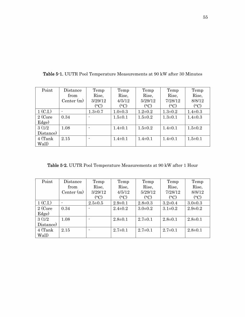
5-1. UUTR Pool Temperature Measurements at 90 kW after 30 Minutes ................ 55
5-2. UUTR Pool Temperature Measurements at 90 kW after 1 Hour........................ 55
5-3. Comparison of Simulation and Temperature Measurements at 90 kW.............. 56
6-1. Values Used in Calculating the Critical Heat Flux ............................................. 65
6-2. Main PARET Input Parameters ........................................................................... 65
6-3. PARET Calculated Maximum Surface Heat Flux ............................................... 66
6-4. UUTR Critical Heat Flux and DNBR at 35°C ..................................................... 66
6-5. PARET Hottest Element Calculated DNB and Cladding Surface
Temperatures ............................................................................................................... 66

vii
7-1. Estimated Costs of Cooling System Replacement ............................................... 79
A-1. Historical UUTR Thermal Power Calibration Data (at 90 kW) [Data from 7] .. 82

ACKNOWLEDGEMENTS
I wish to thank my advisor Dr. Tatjana Jevremovic for her great
encouragement, guidance and assistance in helping me to complete my thesis. I am
also very grateful to Dr. Dong-Ok Choe and Dr. Haori Yang for their assistance and
willingness to help with my research. In addition, I would like to thank my fellow
graduate students Avdo Cutic, Todd Sherman and Jason Rapich for their help and
friendship.
This thesis would not have been possible without the help of my grandfather,
Richard Schanz, who encouraged me to pursue a master’s degree. Also, I am
especially grateful for the support of all my family and my loving wife, Jane.

1
CHAPTER 1
INTRODUCTION
1.1 Thesis Objectives
The University of Utah is home to a TRIGA reactor (UUTR) currently licensed
to operate up to 100 kW. The objective of this thesis is to analyze the
thermohydraulics aspect of increasing the reactor’s power in determining a design
basis area for higher power including the cost estimate. A survey of research
reactors and their cooling systems is conducted and reactor pool conditions are
modeled using SolidWorks Flow Simulation, PARET-ANL and Ansys Fluent.
These results form a basis for the reactor’s power upgrade and the design of its
cooling system.
1.2 Background
The University of Utah TRIGA Reactor has been operating since 1975 without
an incident. The UUTR is a modified TRIGA Mark I pool-type reactor that
currently is operated at a maximum of 90 kW, although licensed to operate at a
maximum power of 100 kW. However, the fuel core design has the potential of
increasing the overall power up to 1 MW.
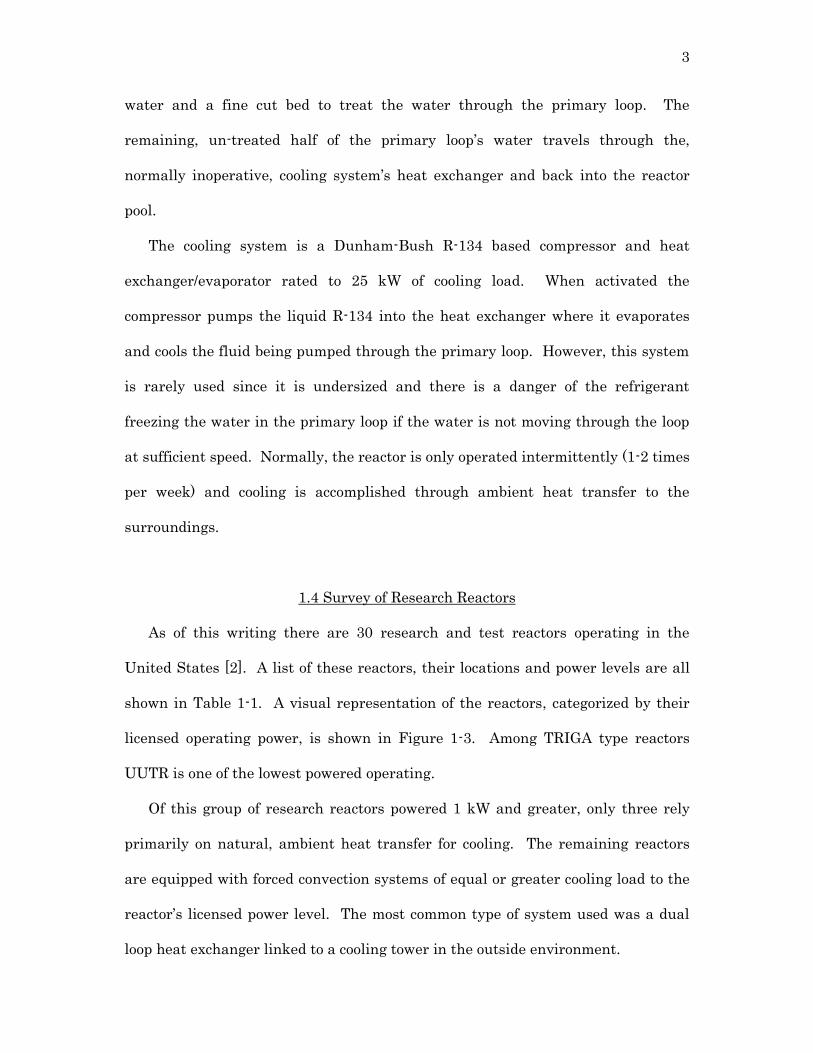
The reactor is located on the first floor of the Merrill Engineering Building at
the University of Utah lower campus. The reactor core is immersed into a deep

2
tank filled with purified water and is mounted a small distance off the bottom of
the vessel. The water in the reactor tank provides cooling, a biological shield and
neutron moderation. The core is of hexagonal shape. Inside the core are rings
containing spaces for fuel or other elements and allowing water to flow.
Surrounding the outside of the aluminum tank vessel is a larger diameter, steel
vessel filled with sand that provides a 2 foot (0.61 meter) barrier between the two
vessels [1]. Figure 1-1 provides a side view of the reactor layout.
The UUTR is operated by trained and NRC licensed staff and students of the
University of Utah Nuclear Engineering Program. The UUTR is utilized in many
ways: to train students on reactor operation and nuclear principles, it provides a
neutron and gamma source for research and is used for neutron activation
analysis. The reactor is as well a major research and community outreach tool;
tours of the facility are conducted educating the public and younger students about
nuclear engineering.
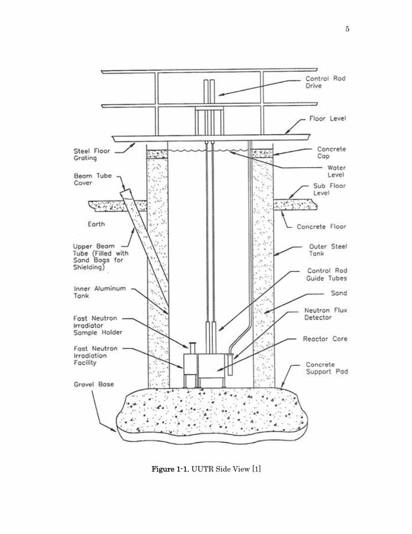
1.3 Current Configuration
The current 100 kW UUTR is cooled using only natural convection. The reactor
pool is filled with deionized water and holds 8,100 gallons of water when full.
When the reactor is operated the heat generated dissipates directly into the pool
water. A primary loop is present off the main pool that deionizes the water and
contains a small cooling system. This loop is driven by an Ingersol-Rand 1-1/2 hp
centrifugal pump creating a 4-6 gpm flow rate. A diagram of the primary loop is
shown in Figure 1-2. Under normal operating conditions, half of the flow is
diverted from the primary loop to pass through the deionizing system. The
deionizer consists of two mixed resin beds: a rough cut bed to treat the make-up
3
water and a fine cut bed to treat the water through the primary loop. The
remaining, un-treated half of the primary loop’s water travels through the,
normally inoperative, cooling system’s heat exchanger and back into the reactor
pool.
The cooling system is a Dunham-Bush R-134 based compressor and heat
exchanger/evaporator rated to 25 kW of cooling load. When activated the
compressor pumps the liquid R-134 into the heat exchanger where it evaporates
and cools the fluid being pumped through the primary loop. However, this system
is rarely used since it is undersized and there is a danger of the refrigerant
freezing the water in the primary loop if the water is not moving through the loop
at sufficient speed. Normally, the reactor is only operated intermittently (1-2 times
per week) and cooling is accomplished through ambient heat transfer to the
surroundings.
1.4 Survey of Research Reactors
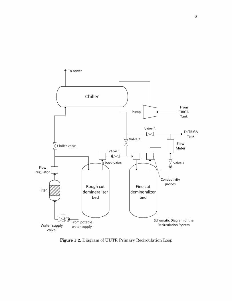
As of this writing there are 30 research and test reactors operating in the
United States [2]. A list of these reactors, their locations and power levels are all
shown in Table 1-1. A visual representation of the reactors, categorized by their
licensed operating power, is shown in Figure 1-3. Among TRIGA type reactors
UUTR is one of the lowest powered operating.
Of this group of research reactors powered 1 kW and greater, only three rely
primarily on natural, ambient heat transfer for cooling. The remaining reactors
are equipped with forced convection systems of equal or greater cooling load to the
reactor’s licensed power level. The most common type of system used was a dual
loop heat exchanger linked to a cooling tower in the outside environment.

4
1.5 Motivation
Thermodynamic calculations and CFD (Computational Fluid Dynamics)
simulations were performed to gain a better understanding of heat flow in the
UUTR water tank. These analyses are necessary to study the feasibility of a power
upgrade for UUTR. The results will help to determine a theoretical, new higher
power level for UUTR and to design a proper forced convection cooling system that
will allow extended reactor operations at the new power level.
5
Figure 1-1. UUTR Side View [1]
6
Figure 1-2. Diagram of UUTR Primary Recirculation Loop
7
Figure 1-3. Operating Research and Test Reactors in the U.S.A. Grouped by Their
Licensed Power [Data from 2]

8
Table 1-1. Operating Research and Test Reactors in the U.S.A. [Data from 2]
Reactor Location City, State Power Cooling System
Aerotest Operations San Ramon, CA 250 kW yes
Armed Forces
Radiobiological Research
Institute
Bethesda, MD 1 MW 1.5 MW
Dow Chemical Midland, MI 300 kW 1 MW
Idaho State University Pocatello, ID 5 W -
Kansas State University Manhattan, KS 1.25 MW 1.25 MW
Massachusetts Institute of
Technology
Cambridge, MA 5 MW 6 MW
National Institute of
Standards and Technology
Gaithersburg, MD 20 MW 22 MW
North Carolina State
University
Raleigh, NC 1 MW yes
Ohio State University Columbus, OH 500 kW 500 kW
Oregon State University Corvallis, OR 1.1 MW 1 MW
Penn State University University Park, PA 1 MW 1 MW
Purdue University West Lafayette, IN 1 kW no
Reed College Portland, OR 250 kW 500 kW
Rensselaer Polytechnic
Institute
Schenectady, NY 1 W (100
W max)
-
Rhode Island Atomic
Energy Commission
Narragansett, RI 2 MW 2.3 MW
Texas A&M College Station, TX 1 MW 2 MW
Texas A&M College Station, TX 5 W -
University of California-
Davis
Davis, CA 2 MW 2 MW
University of California-
Irvine
Irvine, CA 250 kW 258 kW
University of Florida Gainesville, FL 100 kW
(125 kW
max)
500 kW
University of Maryland College Park, MD 250 kW 300 kW
University of
Massachusetts
Lowell, MA 1 MW yes
University of Missouri Columbia, MO 10 MW yes
University of Missouri Rolla, MO 200 kW no
University of New Mexico Albuquerque, NM 5 W -
University of Texas Austin, TX 1 MW yes
University of Utah Salt Lake City, UT 100 kW 25 kW
University of Wisconsin Madison, WI 1 MW 1 MW
U.S. Geological Survey Denver, CO 1 MW 1 MW
Washington State
University
Pullman, WA 1 MW 1.3 MW
9
CHAPTER 2
HEAT TRANSFER PHENOMENA IN UUTR
2.1 Heat Transfer Background
As the reactor is operated energy is released through the fission process. The
majority of this energy appears as energy carried by fission fragments, gamma
rays, neutrons and beta particles emitted [3]. When these particles interact with
the surrounding materials, heat is produced. This process heats up the fuel meat
and starts the chain of heat transfer.
While there has been a great deal of research on heat transfer inside fuel and
on fuel rods for TRIGA reactors [4, 5], this study focuses on the system as a whole.
The fuel rods in the UUTR core heat the surrounding water which flows through
the fuel channels then up and over the rods in a natural convection loop. The
heated water then can either evaporate from the open top of the reactor pool or the
heat is transferred to the environment. Transferring the heat to the environment
can be either through the top surface which is open to the air or through the
aluminum tank wall, sand barrier and outer steel tank wall. Currently, through
one of these two methods is the only way the pool water is cooled back to ambient
temperature.
10
2.2 Energy Equations
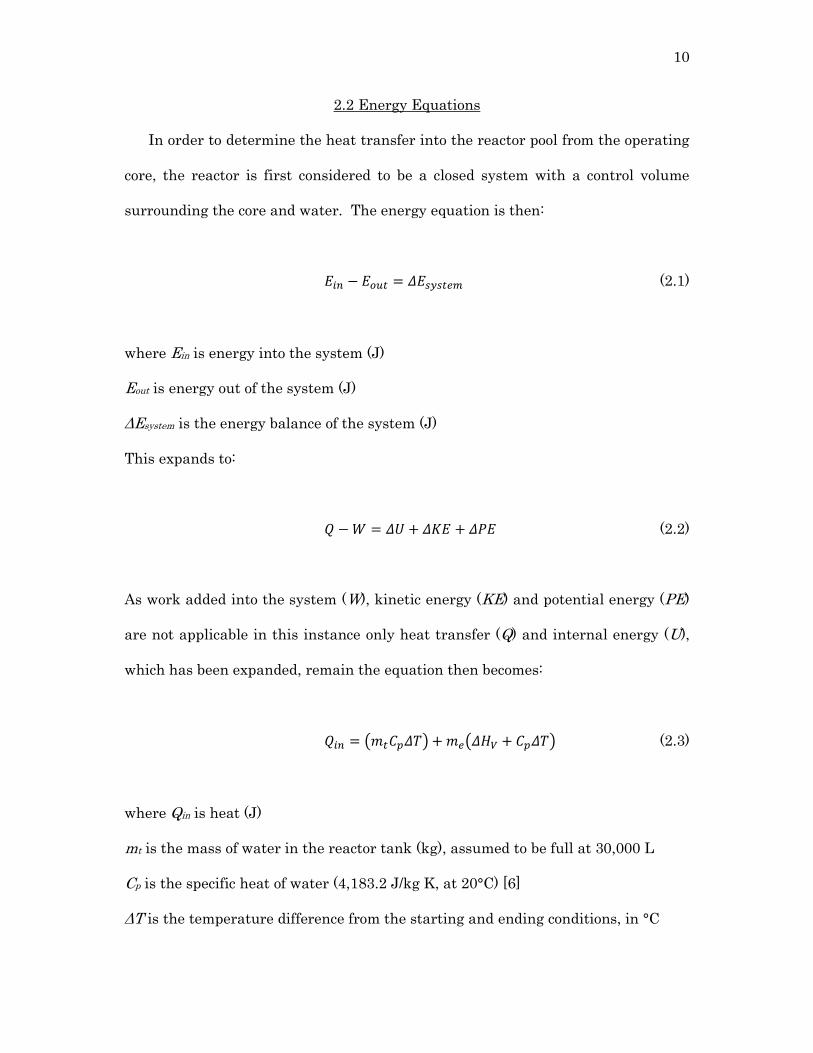
In order to determine the heat transfer into the reactor pool from the operating
core, the reactor is first considered to be a closed system with a control volume
surrounding the core and water. The energy equation is then:
(2.1)
where Ein is energy into the system (J)
Eout is energy out of the system (J)
ΔEsystem is the energy balance of the system (J)
This expands to:
(2.2)
As work added into the system (W), kinetic energy (KE) and potential energy (PE)
are not applicable in this instance only heat transfer (Q) and internal energy (U),
which has been expanded, remain the equation then becomes:
( ) ( ) (2.3)
where Qin is heat (J)
mt is the mass of water in the reactor tank (kg), assumed to be full at 30,000 L
Cp is the specific heat of water (4,183.2 J/kg K, at 20°C) [6]
ΔT is the temperature difference from the starting and ending conditions, in °C
11
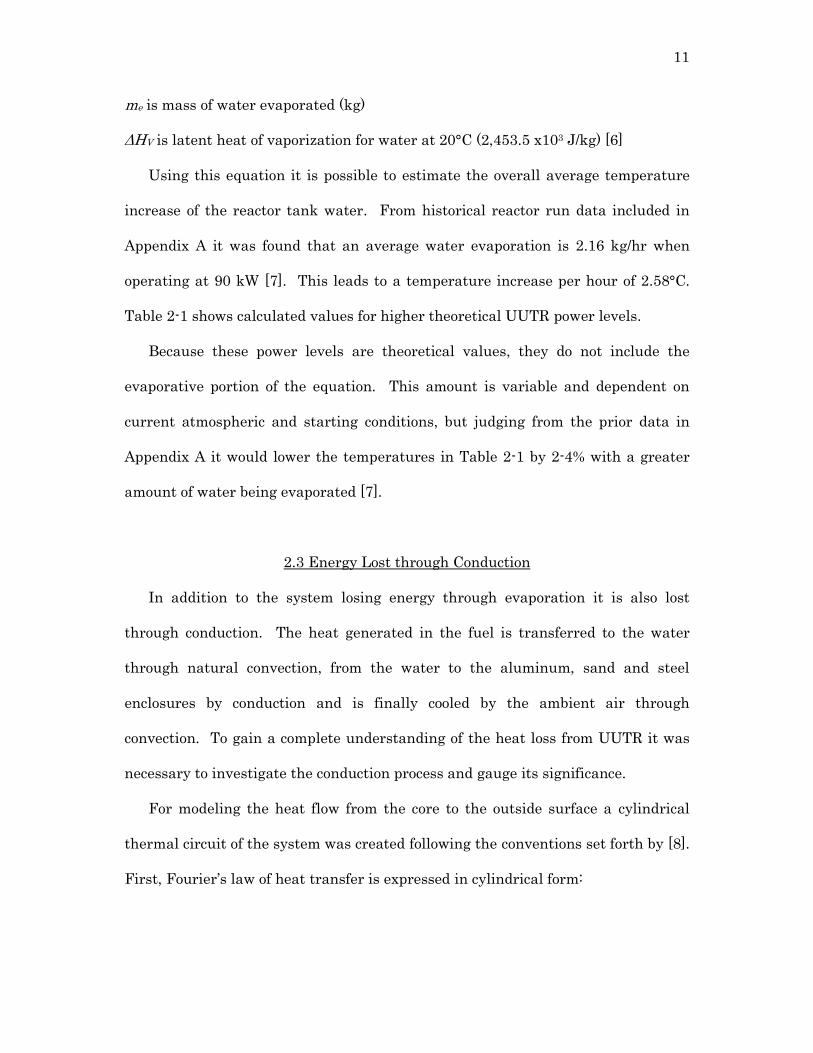
me is mass of water evaporated (kg)
ΔHV is latent heat of vaporization for water at 20°C (2,453.5 x103 J/kg) [6]
Using this equation it is possible to estimate the overall average temperature
increase of the reactor tank water. From historical reactor run data included in
Appendix A it was found that an average water evaporation is 2.16 kg/hr when
operating at 90 kW [7]. This leads to a temperature increase per hour of 2.58°C.
Table 2-1 shows calculated values for higher theoretical UUTR power levels.
Because these power levels are theoretical values, they do not include the
evaporative portion of the equation. This amount is variable and dependent on
current atmospheric and starting conditions, but judging from the prior data in
Appendix A it would lower the temperatures in Table 2-1 by 2-4% with a greater
amount of water being evaporated [7].
2.3 Energy Lost through Conduction
In addition to the system losing energy through evaporation it is also lost
through conduction. The heat generated in the fuel is transferred to the water
through natural convection, from the water to the aluminum, sand and steel
enclosures by conduction and is finally cooled by the ambient air through
convection. To gain a complete understanding of the heat loss from UUTR it was
necessary to investigate the conduction process and gauge its significance.
For modeling the heat flow from the core to the outside surface a cylindrical
thermal circuit of the system was created following the conventions set forth by [8].
First, Fourier’s law of heat transfer is expressed in cylindrical form:
12
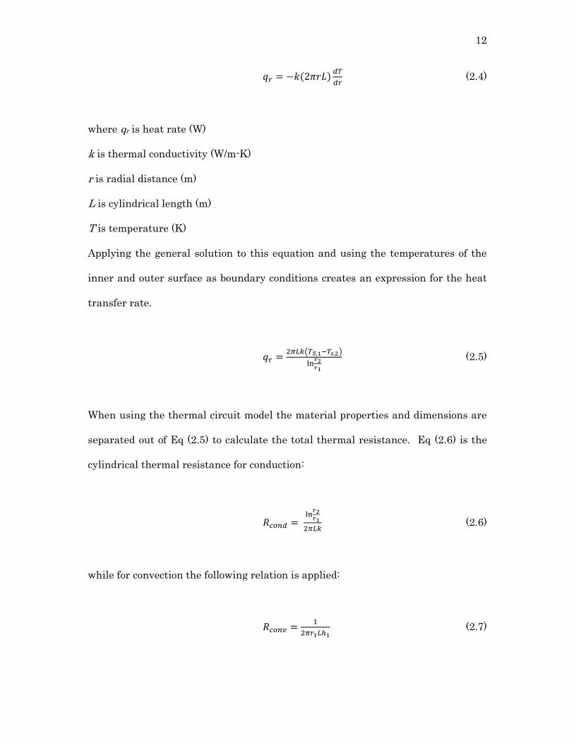
( )
(2.4)
where qr is heat rate (W)
k is thermal conductivity (W/m-K)
r is radial distance (m)
L is cylindrical length (m)
T is temperature (K)
Applying the general solution to this equation and using the temperatures of the
inner and outer surface as boundary conditions creates an expression for the heat
transfer rate.
( )
(2.5)
When using the thermal circuit model the material properties and dimensions are
separated out of Eq (2.5) to calculate the total thermal resistance. Eq (2.6) is the
cylindrical thermal resistance for conduction:
(2.6)
while for convection the following relation is applied:
(2.7)
13
where R is thermal resistance (K/W)
h is heat transfer coefficient (W/m2-K)
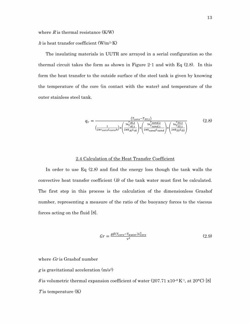
The insulating materials in UUTR are arrayed in a serial configuration so the
thermal circuit takes the form as shown in Figure 2-1 and with Eq (2.8). In this
form the heat transfer to the outside surface of the steel tank is given by knowing
the temperature of the core (in contact with the water) and temperature of the
outer stainless steel tank.
( )
(
) (
) (
) (
)
(2.8)
2.4 Calculation of the Heat Transfer Coefficient
In order to use Eq (2.8) and find the energy loss though the tank walls the
convective heat transfer coefficient (h) of the tank water must first be calculated.
The first step in this process is the calculation of the dimensionless Grashof
number, representing a measure of the ratio of the buoyancy forces to the viscous
forces acting on the fluid [8].
( )
(2.9)
where Gr is Grashof number
g is gravitational acceleration (m/s2)
β is volumetric thermal expansion coefficient of water (207.71 x10⁻⁶ K-1, at 20°C) [8]
T is temperature (K)
14
L is length (m)
ν is kinematic viscosity of water (1.0058 x10⁻⁶ m2/s, at 20°C) [8]
This result is multiplied by the Prandtl number for water at 20°C to give the
Rayleigh number, a measure of the magnitude of buoyancy and viscous forces in
the water.
It was decided to use the heated, upward-facing, flat plate correlation to model
the reactor core. This correlation calculates the ratio of conductive to convective
heat transfer known as the Nusselt number (Nu). Based on the calculated
Rayleigh number and the chosen correlation the following relation is used [8]:
(2.10)
After finding the Nusselt number the heat transfer coefficient (h) can be known
through their relationship derived from Newton’s law of cooling.
(2.11)
where L is the heated length (m)
k is thermal conductivity (W/m-K)
Figure 2-2 summarizes this process and shows the results of each step. After this
value is known the calculation can proceed to obtain the overall thermal resistance
of the reactor system using Eq (2.8).

15
2.5 Calculation of Conduction Heat Loss
The heat transfer coefficient for the reactor tank water, calculated in Section
2.4 to be 704.84 W/m2K, was inserted into Eq (2.8) with the remaining variables
defined in Table 2-2 to calculate the heat lost through conduction. The total
thermal resistance (R) calculated for UUTR was 0.019 K/W. This results in a loss
of 1,590 W of heat through conduction to the outer wall while operating at 90 kW.
2.6 Discussion
When UUTR is at 90 kW, it was found that the typical range for evaporative
energy was 1.8-3.6 kW while only 1.59 kW were transferred through conduction.
These methods only account for a maximum 5.77% of the total power generated.
The remaining continues to heat the tank water through natural convection until it
is eventually removed passively to the environment or actively by a heat
exchanger. In Chapters 3 and 4 the simulations of this heating process in greater
detail are described; the cooling systems are then discussed in Chapter 7.

16
Figure 2-1. Thermal Circuit Diagram for UUTR
Figure 2-2. Process of Determining the Convection Heat Transfer Coefficient

17
Table 2-1. Temperature Increases per Hour for Higher UUTR Power Levels
Power Level (kW) Temperature Rise/Hour
(°C)
100 2.87
200 5.74
300 8.60
400 11.47
500 14.34
Table 2-2. Variables Affecting UUTR Heat Conduction
Variable Description Value (Units)
Tcore Fuel temperature contacting water at 90
kW
53.7 (°C) [1]
TSS,2 Temperature of outer SS wall 23.0 (°C)
rcore Core radius 0.29 (m)
Lcore Core height 0.67 (m)
h Heat transfer coefficient of water 704.84 (W/m2-K)
rAl,1 Inner radius of Al tank 1.17 (m)
rAl,2 Outer radius of Al tank 1.18 (m)
kAl Thermal conductivity of Al 177 (W/m-K) [6]
LAl Height of Al tank 7.32 (m)
rsand,1 Inner radius of sand layer 1.18 (m)
rsand,2 Outer radius of sand layer 1.48 (m)
ksand Thermal conductivity of sand 0.27 (W/m-K) [6]
Lsand Height of sand layer 7.32 (m)
rSS,1 Inner radius of SS tank 1.48 (m)
rSS,2 Outer radius of SS tank 1.485 (m)
kSS Thermal conductivity of SS 14.9 (W/m-K) [6]
LSS Height of SS tank 7.32 (m)
18
CHAPTER 3
SOLIDWORKS BASED ASESSMENT OF UUTR HEAT
TRANSFER AND THERMAL-HYDRAULICS
PHENOMENA
3.1 Introduction
The SolidWorks design software and Flow Simulation package [9] were used to
model the overall setup of the UUTR tank to visualize and quantify the natural
convective cooling process of the core, especially over longer operation. These
results were compared to temperature measurements taken during reactor
operations to help validate the model. The same model is then used to assess the
conditions at higher core power levels.
3.2 SolidWorks and SolidWorks Flow Simulation
SolidWorks is a 3-D computer-aided-design (CAD) software suite currently
developed by Dassault. It allows creation and manipulation of 3-D parts and
assemblies using a parametric design approach. SolidWorks is widely used in
engineering fields for product design, testing and manufacture [10].
SolidWorks Flow Simulation is a fluid dynamics and thermal simulation
program that works through SolidWorks models and assemblies. The software
works using the finite volume (FV) solution method to solve the governing
19
equations over the computational mesh. Because the equations are discretized
over each volume, values for each surface can be known making this method
conservative [11].
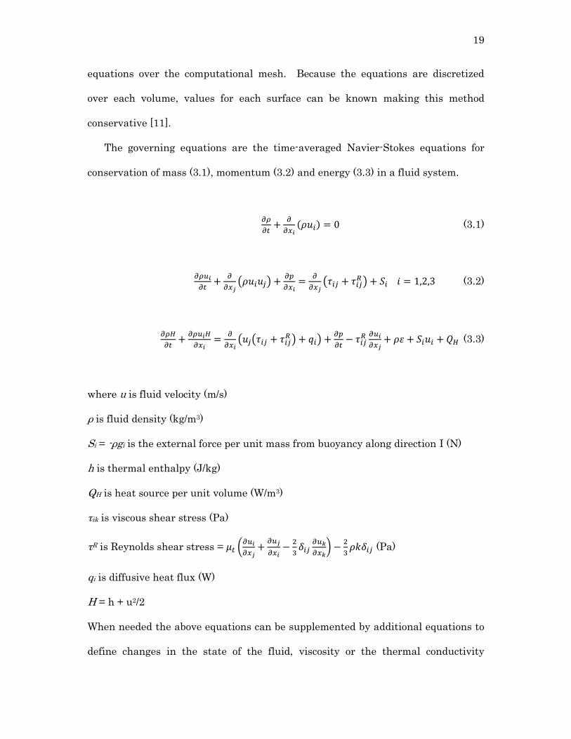
The governing equations are the time-averaged Navier-Stokes equations for
conservation of mass (3.1), momentum (3.2) and energy (3.3) in a fluid system.
( ) (3.1)
( )
(
) (3.2)
( (
) )
(3.3)
where u is fluid velocity (m/s)
ρ is fluid density (kg/m3)
Si = -ρgi is the external force per unit mass from buoyancy along direction I (N)
h is thermal enthalpy (J/kg)
QH is heat source per unit volume (W/m3)
τik is viscous shear stress (Pa)
τR is Reynolds shear stress = (
)
(Pa)
qi is diffusive heat flux (W)
H = h + u2/2
When needed the above equations can be supplemented by additional equations to
define changes in the state of the fluid, viscosity or the thermal conductivity
20
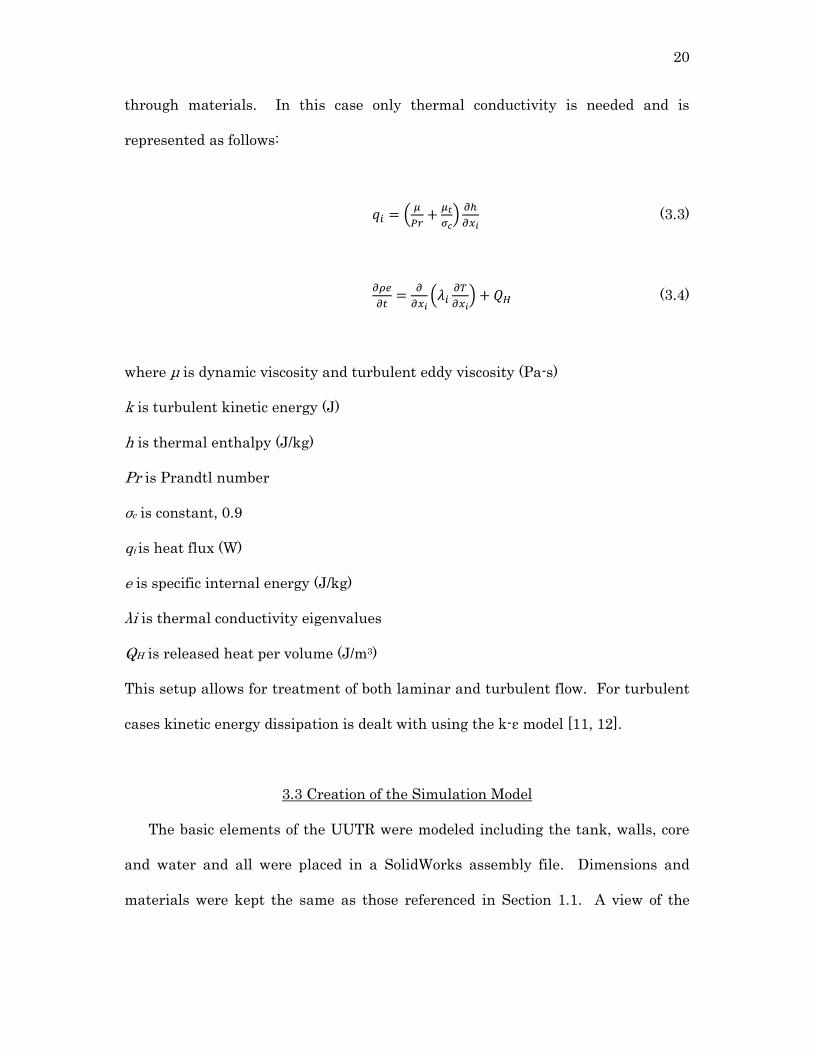
through materials. In this case only thermal conductivity is needed and is
represented as follows:
(
)
(3.3)
(
) (3.4)
where μ is dynamic viscosity and turbulent eddy viscosity (Pa-s)
k is turbulent kinetic energy (J)
h is thermal enthalpy (J/kg)
Pr is Prandtl number
σc is constant, 0.9
qi is heat flux (W)
e is specific internal energy (J/kg)
λi is thermal conductivity eigenvalues
QH is released heat per volume (J/m3)
This setup allows for treatment of both laminar and turbulent flow. For turbulent
cases kinetic energy dissipation is dealt with using the k-ε model [11, 12].
3.3 Creation of the Simulation Model
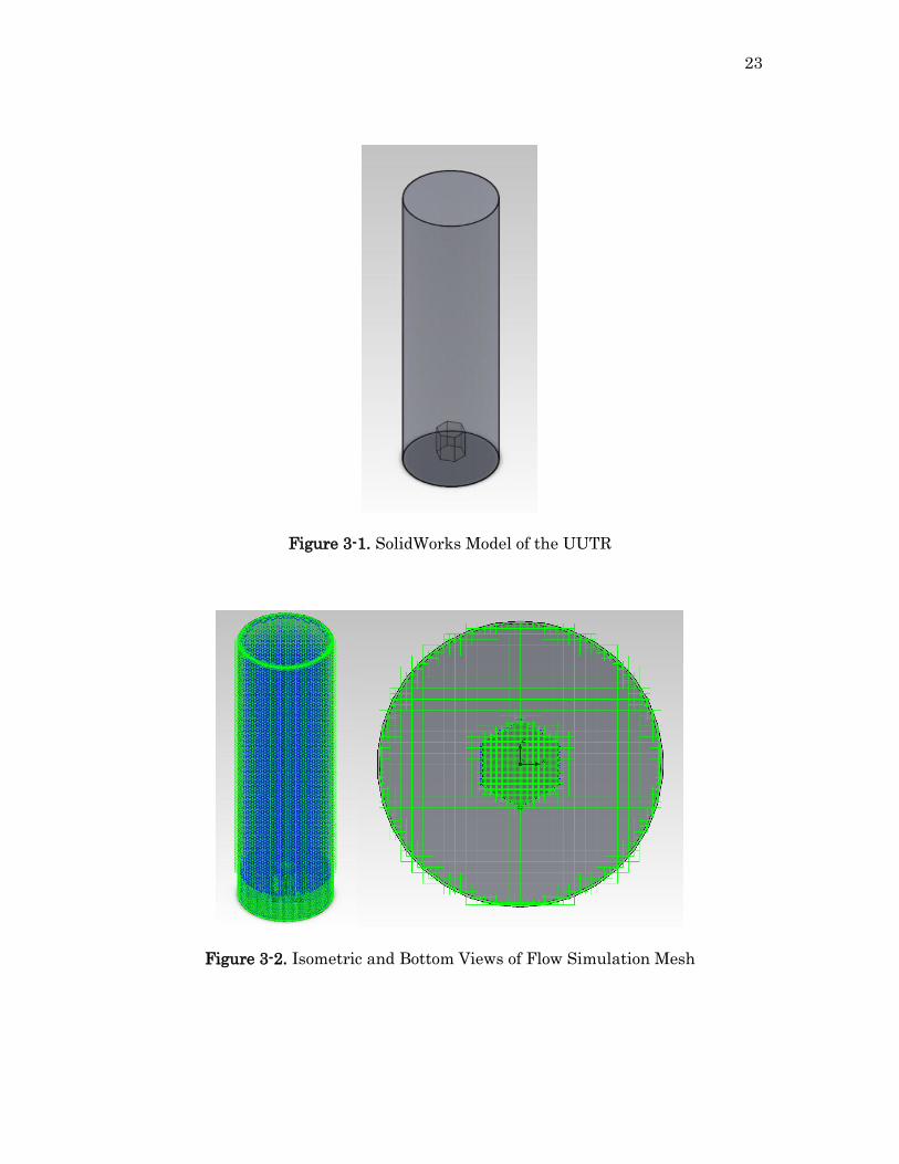
The basic elements of the UUTR were modeled including the tank, walls, core
and water and all were placed in a SolidWorks assembly file. Dimensions and
materials were kept the same as those referenced in Section 1.1. A view of the
21
geometry as built in SolidWorks is shown in Figure 3-1 (walls have been made
transparent for ease of viewing).
Creating the model in this simple fashion allowed for more reasonable
computation times while still achieving the goals of temperature measurement and
flow visualization. In the Flow Simulation software the computational domain was
applied up to the outer wall edge and a 3-D rectangular mesh was selected. Using
mesh refinement a minimum gap size of 0.79 inches (0.02 meters) was specified. It
was found that this size resulted in complete and small enough coverage without
greatly increasing computation times. Images of the created mesh are shown in
Figure 3-2 and the mesh statistics are shown in Table 3-1. The mesh near the
walls and core has a finer resolution for better modeling of the thermal and velocity
boundary layers whereas in the center of the tank the mesh is coarse.
3.4 Flow Simulation Setup
The analysis was carried out using an internal simulation with time
dependency and gravity enabled (-9.81 m/s in the y direction). Water was chosen
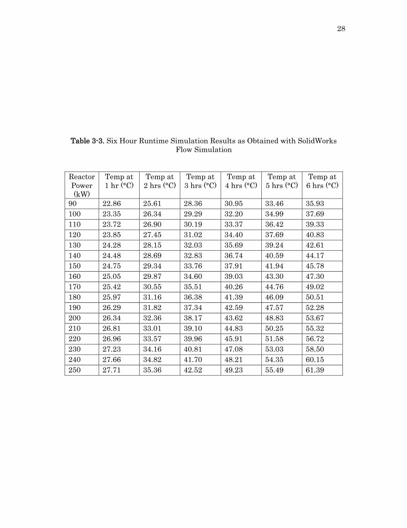
as the working fluid to fill the tank. The variable properties of density, dynamic
viscosity, specific heat (Cp) and thermal conductivity are defined in Table 3-2 over
the range of 20° – 70°C with the software using a linear interpolation for
intermediate values. Starting temperature for the simulations was set at 20°C or
24°C and air pressure at 1 atm.
The interior walls of the aluminum tank were defined to act as a real wall with
the heat transfer coefficient set as -704.84 W/m2-K (negative sign convention,
reference Figure 2-2). The core was defined as a surface heat source with a
constant, overall heat flux equal to the reactor’s power level. Simulation time was
22
set to run for a total of 6 hours (21,600 sec) with results being recorded at each
hour. Global goals were setup in the program to track the fluid temperature and
velocity over the course of the simulation. A complete list of input data for the
simulations is included in Appendix B. The simulations were run on the College of
Engineering’s server, a dual-processor, 64-bit AMD Opteron, dual-core system with
32 GB of RAM and running Windows Server 2008.
3.5 Results
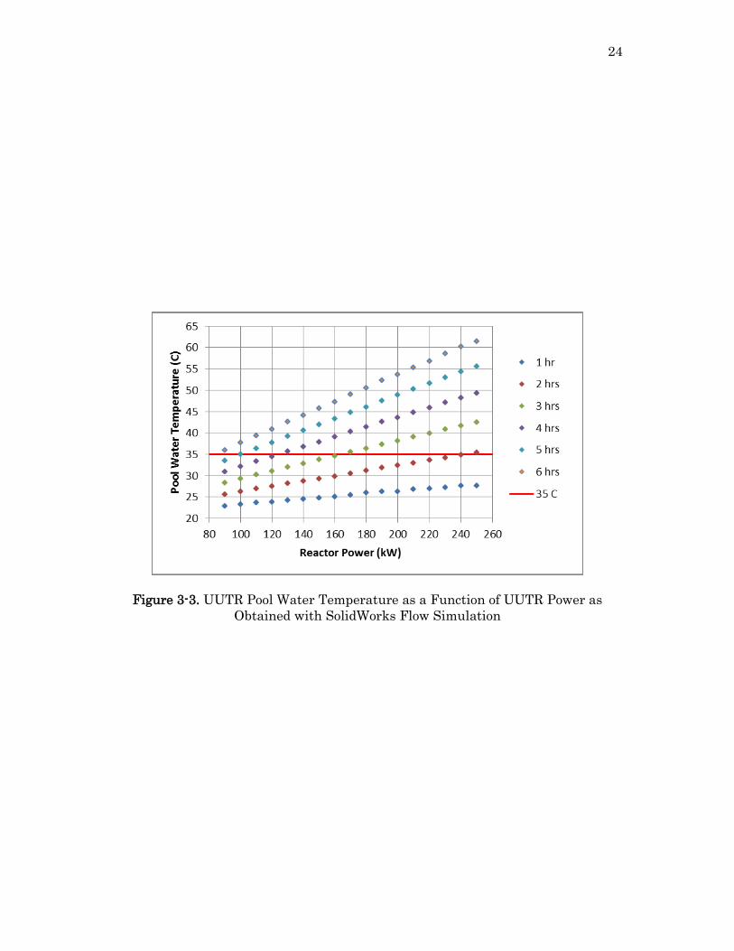
Power levels from 90 to 250 kW were simulated in 10 kW increments for a 6
hour run time. Each was started from an initial temperature of 20°C.
Additionally, a single 90 kW, 1 hour simulation was run with a starting
temperature of 24°C. Temperature measurements were taken at an arbitrary
location 4.5 meters (14.76 feet) from the base of the reactor tank along the center
axis. This location was chosen as it proved to be an area of even temperature
distribution to represent the overall heating of the reactor tank water. The results
from the 20°C simulation are shown plotted in Figure 3-3 and presented in full in
Table 3-3.
Additionally, as a visual aid temperature contour and velocity plots were
created to better compare the 20°C 90 and 250 kW simulations. These are shown
in Figures 3-4 and 3-5. Both temperature contour plots show the more uniform
temperature distribution that is present in the SolidWorks simulations that leads
to more accurate temperature results. The velocity plots both show examples of
vortex shedding caused by fluid movement over the core surface with the 250 kW
core having a more pronounced effect from the higher fluid velocities in the
convection column.
23
Figure 3-1. SolidWorks Model of the UUTR
Figure 3-2. Isometric and Bottom Views of Flow Simulation Mesh
24
Figure 3-3. UUTR Pool Water Temperature as a Function of UUTR Power as
Obtained with SolidWorks Flow Simulation

25
Figure 3-4. Temperature and Velocity Contours at 90 kW after 1 Hour Runtime

26
Figure 3-5. Temperature and Velocity Contours at 250 kW after 1 Hour Runtime
27
Table 3-1. Flow Simulation Mesh Statistics
Cell Type Number
Fluid Cells 70,800
Solid Cells 17,080
Partial Cells 27,840
Total 115,720
Table 3-2. Variable Properties of Water
Temperature
(°C)
Density
(kg/m3)
Dynamic
Viscosity
(Pa-s)
Specific Heat
(J/kg-K)
Thermal
Conductivity
(W/m-K)
20 998.16 1.0014 x10⁻³ 4,184.4 0.59843
25 997.00 8.8990 x10⁻⁴ 4,181.6 0.60717
30 995.60 7.9719 x10⁻⁴ 4,180.1 0.61547
35 993.99 7.1917 x10⁻⁴ 4,179.5 0.62330
40 992.17 6.5285 x10⁻⁴ 4,179.6 0.63060
45 990.17 5.9595 x10⁻⁴ 4,180.4 0.63736
50 987.99 5.4674 x10⁻⁴ 4,181.6 0.64356
55 985.65 5.0388 x10⁻⁴ 4,183.2 0.64923
60 983.16 4.6631 x10⁻⁴ 4,185.1 0.65436
65 980.15 4.3318 x10⁻⁴ 4,187.5 0.65897
70 977.73 4.0382 x10⁻⁴ 4,190.2 0.66310
28
Table 3-3. Six Hour Runtime Simulation Results as Obtained with SolidWorks
Flow Simulation
Reactor
Power
(kW)
Temp at
1 hr (°C)
Temp at
2 hrs (°C)
Temp at
3 hrs (°C)
Temp at
4 hrs (°C)
Temp at
5 hrs (°C)
Temp at
6 hrs (°C)
90 22.86 25.61 28.36 30.95 33.46 35.93
100 23.35 26.34 29.29 32.20 34.99 37.69
110 23.72 26.90 30.19 33.37 36.42 39.33
120 23.85 27.45 31.02 34.40 37.69 40.83
130 24.28 28.15 32.03 35.69 39.24 42.61
140 24.48 28.69 32.83 36.74 40.59 44.17
150 24.75 29.34 33.76 37.91 41.94 45.78
160 25.05 29.87 34.60 39.03 43.30 47.30
170 25.42 30.55 35.51 40.26 44.76 49.02
180 25.97 31.16 36.38 41.39 46.09 50.51
190 26.29 31.82 37.34 42.59 47.57 52.28
200 26.34 32.36 38.17 43.62 48.83 53.67
210 26.81 33.01 39.10 44.83 50.25 55.32
220 26.96 33.57 39.96 45.91 51.58 56.72
230 27.23 34.16 40.81 47.08 53.03 58.50
240 27.66 34.82 41.70 48.21 54.35 60.15
250 27.71 35.36 42.52 49.23 55.49 61.39
29
CHAPTER 4
FLUENT MODEL OF THE UUTR
4.1 Introduction
The Fluent simulation package from Ansys [13] was used to create a more
detailed model of the UUTR core. This model simulated the UUTR tank convection
processes over higher power levels but a shorter time frame. The model was also
validated with temperature measurements taken during normal operations.
4.2 Ansys Fluent
Fluent is a computational fluid dynamics (CFD) code currently developed by
Ansys. The code supports 2-D or 3-D model meshes and provides comprehensive
simulation capabilities for a wide range of incompressible and compressible,
laminar and turbulent fluid flow problems. Simulations can be steady-state or
transient and also includes the ability to model various forms of heat transfer such
as conjugate, radiation and convection [14]. Fluent is commonly used in product
design and optimization and as a tool in thermodynamics and fluidics research.
For this analysis Fluent was used inside the commercially packaged Ansys
Workbench platform.
The software is based on the finite element method (FEM). A computational
mesh is generated for the model being analyzed with the defining equations
30
applied over each mesh element. Boundary conditions are defined at all mesh
edges (walls) creating a conservative system where individual element values can
be known [14].
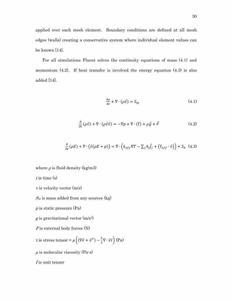
For all simulations Fluent solves the continuity equations of mass (4.1) and
momentum (4.2). If heat transfer is involved the energy equation (4.3) is also
added [14].
( ) (4.1)
( ) ( ) ( ) (4.2)
( ) ( ( )) ( ∑ ( )) (4.3)
where ρ is fluid density (kg/m3)
t is time (s)
v is velocity vector (m/s)
Sm is mass added from any sources (kg)
p is static pressure (Pa)
g is gravitational vector (m/s2)
F is external body forces (N)
τ is stress tensor = (( )
) (Pa)
µ is molecular viscosity (Pa-s)
I is unit tensor
31
keff is effective conductivity (S/m)
J is the diffusion flux of j (kg/m2-s)
Sh is energy from external or volumetric heat sources (J)
E =
h is enthalpy (J/kg)
As with the Flow Simulation software, Fluent can model many other fluid and
thermodynamic conditions as the user activates add-on equations.
4.3 Creation of the Fluent Model
The tank, walls, core and water of UUTR were modeled to their original
dimensions (as reported in Section 1.1) in the DesignModeler program included
with the Ansys simulation package. During this process the UUTR core was
further discretized into zones so that the pin power distribution could be mapped to
the surface. The 3-D model is shown in Figure 4.1.
In the Ansys meshing program the created geometry was opened and a
tetrahedral shaped mesh and CFD physics preference were chosen. A coarse
relevance center was used with medium smoothing and a slow transition area
around the core for increased flow detail in that region. The generated mesh is
shown in Figure 4-2 and its statistics are presented in Table 4.1. After the mesh
was created all of the wall faces and discretized core sections were named to
facilitate their recognition by Fluent. The mesh was then loaded into the Fluent
solver.

32
4.4 Fluent Simulation
In the Fluent software the imported mesh is checked for connectivity and
correct volume. Then the solver is set to perform a pressure-based, absolute,
transient simulation with gravity enabled (-9.81 m/s2 in the y direction). For this
simulation the energy equation is enabled and the laminar model is used. In the
materials section the fluid is set to liquid water and the solid materials are defined
to be aluminum. The properties specified for each of these materials (at 20°C) are
shown in Table 4-2. Also, water density was defined to follow a Boussinesq
approximation. The Boussinesq model for natural convection flows gives faster
convergence than having the fluid density as a function of temperature. The model
assumes fluid density is constant in all solved equations except in the momentum
Eq (4.2) where it is replaced by Eq (4.4). The approximation is accurate as long as
β(T-T0)<<1 which applies for all cases during these simulations [15].
( ) (4.4)
where ρ is new density (kg/m3)
ρ0 is constant density (kg/m3)
β is thermal expansion coefficient of water (207 x10-6 K-1)
The next step involves defining the cell zones and boundary conditions. Under
the Cell Zone Conditions section the interior zone is changed to a fluid and edited
to contain the water defined in the above steps. In the Boundary Conditions
section all named wall sections created in the meshing process appear. The side
and bottom tank walls are defined as convection/conduction boundaries between
33
the water and aluminum while the top is defined as a convection boundary open to
the atmosphere. Both use the heat transfer coefficient defined in Ch. 2 and specify
a room temperature of 22°C. The core surfaces are defined as thermal boundaries
with a heat flux. Following the same practice as in the Safety Analysis Report
(SAR) [1], the core was discretized into sixths for entry into the software as shown
in Figure 4-3 to facilitate the power mapping onto the thermal boundaries in the
model.
To increase simulation speed and aid in modeling, the top and bottom surfaces
were divided into ring sections corresponding to the fuel element rings to aid in
mapping the power distribution to the thermal boundaries. The pin power
distributions [1, 16] and core surface area were used to determine the heat flux as
follows:
(4.5)
The process of dividing the core up into sections and then using the pin power
distributions to calculate the heat flux for each thermal boundary was repeated for
each power lever that was simulated. The heat flux values varied based on the
total reactor power and core layout.
Analysis was carried out using the Pressure Implicit with Splitting of
Operators (PISO) solution algorithm with the spatial discretization of pressure set
to second order, the recommended settings for buoyancy driven flows. This
solution method assumes a higher degree of relation between the corrections for
pressure and velocity and can greatly reduce the number of iterations required for
34
convergence, especially in transient cases [14]. The remainder of the solution
settings were left at the default values and are listed in their entirety in Appendix
C. Under-relaxation factors for the solution controls were also left at the default
values. The solution was initialized to start at a temperature of either 20°C
(293°K) or 24°C (297°K) and calculation activities were set up to record fluid
temperature and velocity at 5 minute intervals. After this setup the solver was run
with a 1 second time step until a maximum simulation time of 3,600 seconds was
reached. All simulations were run on the College of Engineering’s server, a dual-
processor, 64-bit AMD Opteron, dual-core system with 32 GB of RAM and running
Windows Server 2008.
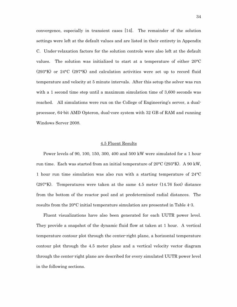
4.5 Fluent Results
Power levels of 90, 100, 150, 300, 400 and 500 kW were simulated for a 1 hour
run time. Each was started from an initial temperature of 20°C (293°K). A 90 kW,
1 hour run time simulation was also run with a starting temperature of 24°C
(297°K). Temperatures were taken at the same 4.5 meter (14.76 foot) distance
from the bottom of the reactor pool and at predetermined radial distances. The
results from the 20°C initial temperature simulation are presented in Table 4-3.
Fluent visualizations have also been generated for each UUTR power level.
They provide a snapshot of the dynamic fluid flow at taken at 1 hour. A vertical
temperature contour plot through the center-right plane, a horizontal temperature
contour plot through the 4.5 meter plane and a vertical velocity vector diagram
through the center-right plane are described for every simulated UUTR power level
in the following sections.

35
4.5.1. Fluent 1 Hour Temperature and Velocity for the 90 kW Core
Figure 4.4 is the temperature contour plot from the center-right, vertical plane
showing the 90 kW core’s convection current as it rises over the height of the
reactor pool. Figure 4.5 is the temperature contour plot from the 4.5 meter,
horizontal plane showing the distribution of the convection current at 4.5 meters
above the pool’s base. Figure 4.6 is the velocity vector plot from the center-right,
vertical plane showing the water velocity in the rising convection current of the 90
kW core.
4.5.2. Fluent 1 Hour Temperature and Velocity for the 100 kW Core
The temperature contour plot at the center-right, vertical plane showing the
100 kW core’s convection current as it rises over the height of the reactor pool is
shown in Figure 4.7. Figure 4.8 depicts the temperature contour plot at the 4.5
meter, horizontal plane showing the distribution of the convection current at 4.5
meters above the pool’s base. Figure 4.9 shows the velocity vector plot from the
center-right, vertical plane showing the water velocity in the rising convection
current of the 100 kW core.
4.5.3. Fluent 1 Hour Temperature and Velocity for the 150 kW Core
Figure 4.10 is the temperature contour plot at the center-right, vertical plane
showing the 150 kW core’s convection current as it rises over the height of the
reactor pool. Figure 4.11 shows the temperature contour plot at the 4.5 meter,
horizontal plane showing the distribution of the convection current at 4.5 meters
above the pool’s base. Figure 4.12 shows the velocity vector from the center-right,
36
vertical plane showing the water velocity in the rising convection current of the 150
kW core.
4.5.4. Fluent 1 Hour Temperature and Velocity for the 300 kW Core
The temperature contour plot at the center-right, vertical plane showing the
300 kW core’s convection current as it rises over the height of the reactor pool is
shown in Figure 4.13, while Figure 4.14 shows the temperature contour plot at the
4.5 meter height horizontal plane. Figure 4.15 depicts the velocity vector plot from
the center-right, vertical plane showing the water velocity in the rising convection
current of the 300 kW core.
4.5.5. Fluent 1 Hour Temperature and Velocity for the 400 kW Core
Figure 4.16 captures the temperature contours at the center-right, vertical
plane of the 400 kW core’s convection current moving up the height of the reactor
pool and Figure 4.17 shows the temperature contour plot at the 4.5 meter
horizontal plane. Figure 4.18 is the velocity vector plot from the center-right,
vertical plane of the water velocity in the convection current of the 400 kW core.
4.5.6. Fluent 1 Hour Temperature and Velocity for the 500 kW Core
Figure 4.19 shows the temperature contour plot at the center-right, vertical
plane of the 500 kW core’s convection current and Figure 4.20 shows the
temperature contour plot at the 4.5 meter height horizontal plane. Figure 4.21
depicts the velocity vector plot from the center-right, vertical plane showing the
water velocity in the convection current of the 500 kW core.

37
Figure 4-1. UUTR Model in Fluent
Figure 4-2. External Surfaces of Fluent Mesh
38
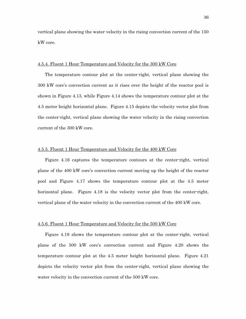
Figure 4-3. Discretizing the Core Sides Prior to Simulation (90 kW Core) [1]
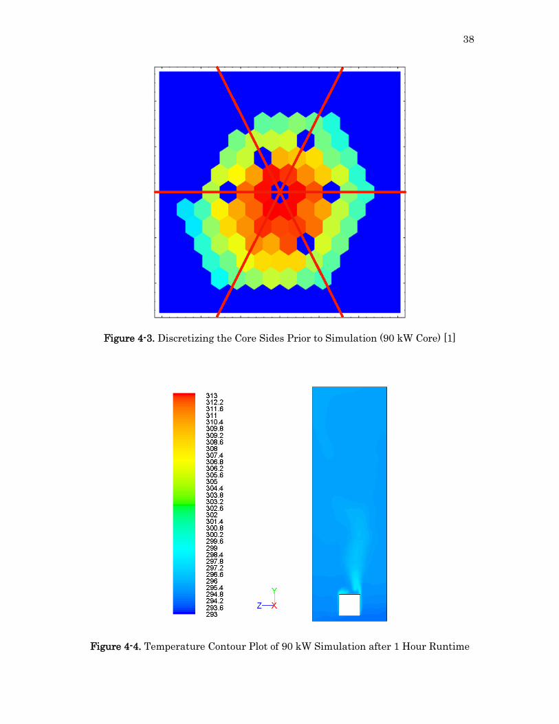
Figure 4-4. Temperature Contour Plot of 90 kW Simulation after 1 Hour Runtime

39
Figure 4-5. Temperature Contour Plot of 90 kW Simulation after 1 Hour Runtime,
4.5 meter Plane
Figure 4-6. Velocity Vector Plot of 90 kW Simulation after 1 Hour Runtime
40
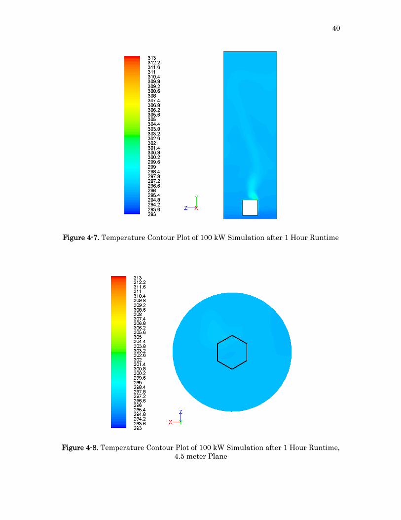
Figure 4-7. Temperature Contour Plot of 100 kW Simulation after 1 Hour Runtime
Figure 4-8. Temperature Contour Plot of 100 kW Simulation after 1 Hour Runtime,
4.5 meter Plane
41
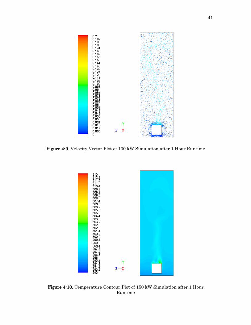
Figure 4-9. Velocity Vector Plot of 100 kW Simulation after 1 Hour Runtime
Figure 4-10. Temperature Contour Plot of 150 kW Simulation after 1 Hour
Runtime

42
Figure 4-11. Temperature Contour Plot of 150 kW Simulation after 1 Hour
Runtime, 4.5 meter Plane
Figure 4-12. Velocity Vector Plot of 150 kW Simulation after 1 Hour Runtime

43
Figure 4-13. Temperature Contour Plot of 300 kW Simulation after 1 Hour
Runtime
Figure 4-14. Temperature Contour Plot of 300 kW Simulation after 1 Hour
Runtime, 4.5 meter Plane
44
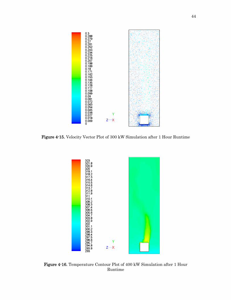
Figure 4-15. Velocity Vector Plot of 300 kW Simulation after 1 Hour Runtime
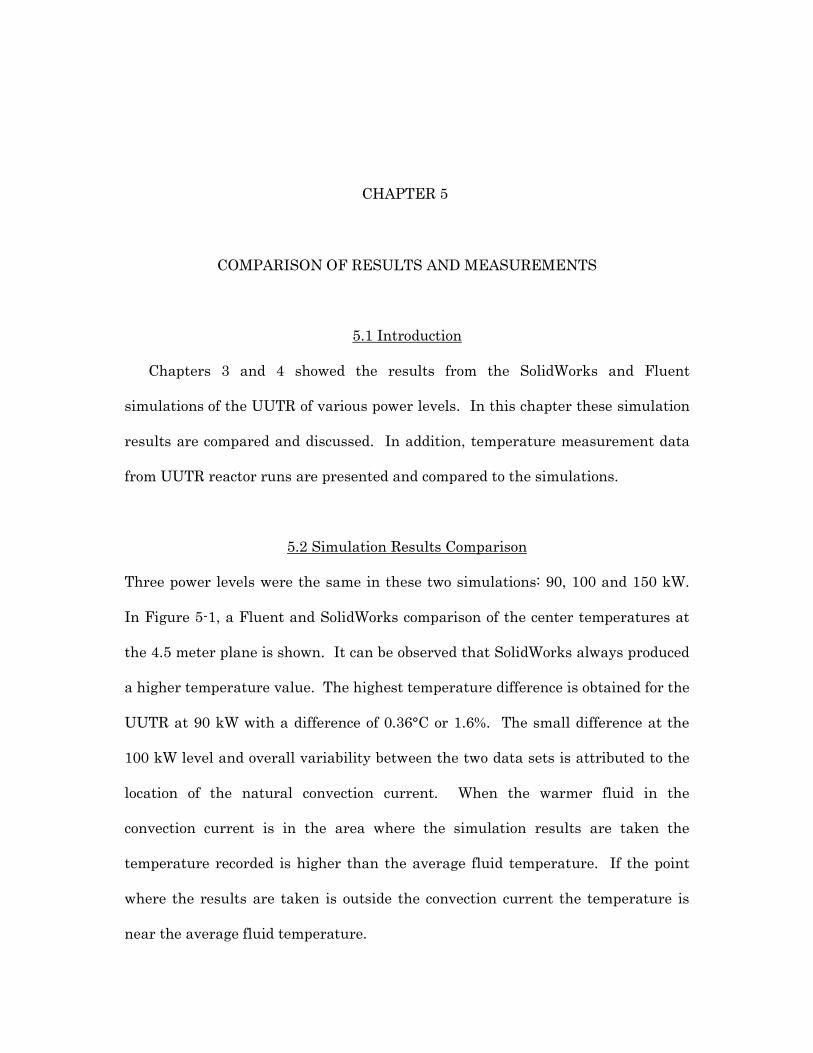
Figure 4-16. Temperature Contour Plot of 400 kW Simulation after 1 Hour
Runtime

45
Figure 4-17. Temperature Contour Plot of 400 kW Simulation after 1 Hour
Runtime, 4.5 meter Plane
Figure 4-18. Velocity Vector Plot of 400 kW Simulation after 1 Hour Runtime

46
Figure 4-19. Temperature Contour Plot of 500 kW Simulation after 1 Hour
Runtime
Figure 4-20. Temperature Contour Plot of 500 kW Simulation after 1 Hour
Runtime, 4.5 meter Plane

47
Figure 4-21. Velocity Vector Plot of 500 kW Simulation after 1 Hour Runtime

48
Table 4-1. Fluent Mesh Statistics
Type Number
Cells 329,024
Faces 668,208
Nodes 60,094
Face Zones 22
Table 4-2. Fluent Material Properties
Material Density
(kg/m3)
Viscosity
(Pa-s)
Specific Heat
(J/kg-K)
Thermal
Conductivity
(W/m-K)
Aluminum 2,719 - 871 202.4
Water (liquid) 998.2 0.001003 4,182 0.6
Table 4-3. Fluent 1 Hour Runtime Simulation Temperature Results
Reactor
Power (kW)
Temp rise at
center (°C)
Temp rise at
core edge (°C)
Temp rise at 1/2
distance (°C)
Temp rise at
tank wall (°C)
90 2.5 2.7 2.5 2.5
100 3.3 3.3 3.2 3.0
150 4.5 4.3 4.3 4.3
300 10.4 9.7 9.7 9.4
400 12.4 12.4 12.4 12.2
500 16.2 16.9 15.3 15.0
49
CHAPTER 5
COMPARISON OF RESULTS AND MEASUREMENTS
5.1 Introduction
Chapters 3 and 4 showed the results from the SolidWorks and Fluent
simulations of the UUTR of various power levels. In this chapter these simulation
results are compared and discussed. In addition, temperature measurement data
from UUTR reactor runs are presented and compared to the simulations.
5.2 Simulation Results Comparison
Three power levels were the same in these two simulations: 90, 100 and 150 kW.
In Figure 5-1, a Fluent and SolidWorks comparison of the center temperatures at
the 4.5 meter plane is shown. It can be observed that SolidWorks always produced
a higher temperature value. The highest temperature difference is obtained for the
UUTR at 90 kW with a difference of 0.36°C or 1.6%. The small difference at the
100 kW level and overall variability between the two data sets is attributed to the
location of the natural convection current. When the warmer fluid in the
convection current is in the area where the simulation results are taken the
temperature recorded is higher than the average fluid temperature. If the point
where the results are taken is outside the convection current the temperature is
near the average fluid temperature.
50
The two models both show the near constant upward slope of increasing
temperature versus reactor power as expected. The Fluent model shows more
variation since the core was discretized according to fuel element levels. The
asymmetrical layout of the core leads to a more unstable and mobile convection
column causing more variation in the temperature results. The SolidWorks model
used a constant, volume type power source and thus had less water movement with
a more stable, uniform convection column. The Fluent model more accurately
models the actual water flow while the SolidWorks model better shows the overall
average temperature.
5.3 UUTR Temperature Measurements
The UUTR pool water temperature is measured with the readings taken at 4.5
meter (14.76 foot) distance from the bottom of the reactor pool and at the
predetermined radial distances as shown in Figure 5-2. The side chosen for the
edge measurements was near fuel element location G-19 because of its higher flux
and ease of measurement access. During normal 90 kW reactor operations three
temperature measurements were taken: during startup, after 30 minutes runtime,
and after 1 hour runtime. A type K thermocouple attached to an Omega TrueRMS
Super Meter was used for collecting all the data. The thermocouple was lowered
into the desired position, allowed to acclimate for 1 minute and then the detected
temperature range was recorded. Before use the Omega Super Meter was
calibrated using the Omega Instruments thermocouple calibration meter and was
found to be operating normally.
The results from the pool water measurements are summarized in Tables 5-1
and 5-2 (Note: the first trial was only conducted in the central location). All of the
51
measurements show some variation between readings. This variation is caused by
the following four reasons:
The first and most important is the location of the convection current. The
flow around the core begins to exhibit vortex shedding once it has
developed. This moves the convection current of heated water back and
forth around the middle area of the reactor pool (as can be evidenced in the
Fluent results in Chapter 4). If the thermal column is away from the point
of measurement at the time readings are taken the temperature will be
lower since the surroundings were measured and not the heated water
directly from the core.
The temperature is also affected by the humans measuring and operating
the UUTR. At UUTR the reactor power is manually controlled by the
operator. While each trial was conducted at 90 kW there is slight variation.
Because of this, it is easy to expect a variation of 90±1 kW. Over longer
periods of time small changes in the power can create slight differences in
the temperature between the measurements.
The operator also controls the rate the reactor power is increased before
reaching the level of 90 kW. Ideally the power would be ramped to the
desired level instantaneously. However, in practice this operation can take
a few minutes or longer depending on the current conditions and
experiments conducted. This time spent ramping up to power still increases
tank water temperature and has an effect on the temperature
measurements.

52
Finally, the temperature is affected by the ambient starting conditions.
During the summer the reactor room temperature is higher causing the
starting pool water temperature to also be higher. From freezing to 35°C
the water’s heat capacity (Cp) slightly decreases, making it easier to heat.
This is evidenced in the two starting temperatures (20°C and 24°C) of both
the SolidWorks and Fluent simulations where the 90 kW, 24°C simulation
more closely matches the measurements taken.
5.4 Simulation and Temperature Measurement Comparison
Currently only results from the 90 kW power level are comparable among the
simulations and measurements. Table 5-3 summarizes these results. There is
close correlation between both of the models used and the actual measurements.
Since the actual measurements were taken during the summer months when
ambient temperature is higher the 24°C simulations are a closer approximation
then the 20°C simulations. The temperature range between the data can be
attributed to the location of the convection current as discussed previously.
Because the Fluent simulations contain a more accurate model of the asymmetrical
core the convection current is more obvious. It is also expected that not every
measurement would capture readings from the inside the convection current.
These results show that a series of measurements are necessary to gauge the
temperature rise in UUTR and that while it local variability is seen overall the
temperature rise follows predictable trends.
53
5.5 UUTR of Higher Power Levels
The simulation of UUTR at higher power levels show that the reactor
undergoes the same natural convective cooling process only the effects become
more pronounced. In the 90 kW simulation the open water fluid velocity peaked at
0.0988 m/s while in the 500 kW simulation the maximum velocity has increased to
0.156 m/s. These results are similar, only more conservative, to those reported in
the SAR which reports 0.115 m/s for 90 kW and 0.130 m/s for 100 kW [1]. The
slower velocities can be attributed to the simpler reactor core models used in both
simulations. These models did not include the coolant channels through the center
of the reactor and around each element. If these channels were included additional
convection heating would occur increasing the velocities.
The other aspect that is seen in the simulations and becomes more pronounced
at higher power levels is the vortex shedding in the convection current above the
reactor core. Because of its asymmetrical power distribution and acting as a blunt
body in the flow field the core creates vortices that travel up the convection column.
The vortices cause the movement of the convection column around the reactor pool.
As the convection current and velocities increase with higher power levels the
vortices also grow and affect the current to a greater extent.

54
Figure 5-1. Comparison of SolidWorks and Fluent Centerline Temperatures on the
4.5 meter Plane
Figure 5-2. Radial Locations of Temperature Measurements in the UUTR
55
Table 5-1. UUTR Pool Temperature Measurements at 90 kW after 30 Minutes
Point Distance
from
Center (m)
Temp
Rise,
3/29/12
(°C)
Temp
Rise,
4/5/12
(°C)
Temp
Rise,
5/29/12
(°C)
Temp
Rise,
7/28/12
(°C)
Temp
Rise,
8/8/12
(°C)
1 (C.I.) - 1.3±0.7 1.0±0.3 1.2±0.2 1.3±0.2 1.4±0.3
2 (Core
Edge)
0.34 - 1.5±0.1 1.5±0.2 1.3±0.1 1.4±0.3
3 (1/2
Distance)
1.08 - 1.4±0.1 1.5±0.2 1.4±0.1 1.5±0.2
4 (Tank
Wall)
2.15 - 1.4±0.1 1.4±0.1 1.4±0.1 1.5±0.1
Table 5-2. UUTR Pool Temperature Measurements at 90 kW after 1 Hour
Point Distance
from
Center (m)
Temp
Rise,
3/29/12
(°C)
Temp
Rise,
4/5/12
(°C)
Temp
Rise,
5/29/12
(°C)
Temp
Rise,
7/28/12
(°C)
Temp
Rise,
8/8/12
(°C)
1 (C.I.) - 2.5±0.5 2.9±0.1 2.8±0.3 3.2±0.4 3.0±0.3
2 (Core
Edge)
0.34 - 2.4±0.2 3.0±0.2 3.1±0.2 2.9±0.2
3 (1/2
Distance)
1.08 - 2.8±0.1 2.7±0.1 2.8±0.1 2.8±0.1
4 (Tank
Wall)
2.15 - 2.7±0.1 2.7±0.1 2.7±0.1 2.8±0.1

56
Table 5-3. Comparison of Simulation and Temperature Measurements at 90 kW
C.I. Point
Temp Rise
(°C)
Core Edge
Temp Rise
(°C)
1/2 Distance
Temp Rise
(°C)
Tank Wall
Temp Rise
(°C)
UUTR
3/29/12
2.5±0.5 - - -
UUTR 4/5/12 2.9±0.1 2.4±0.2 2.8±0.1 2.7±0.1
UUTR
5/29/12
2.8±0.3 3.0±0.2 2.7±0.1 2.7±0.1
UUTR
7/28/12
3.2±0.4 3.1±0.2 2.8±0.1 2.7±0.1
UUTR 8/8/12 3.0±0.3 2.9±0.2 2.8±0.1 2.8±0.1
Fluent (20°C) 2.54 2.73 2.51 2.50
SolidWorks
(20°C)
2.86 2.90 2.82 2.80
Fluent (24°C) 3.11 2.98 2.97 2.73
SolidWorks
(24°C)
2.96 2.95 2.90 2.68

57
CHAPTER 6
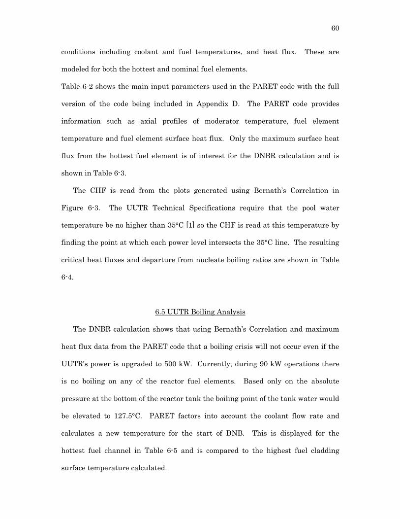
DEPARTURE FROM NUCLEATE BOILING RATIO
6.1 Introduction
This chapter describes the departure from nucleate boiling in UUTR in showing
that even at higher power levels the heat flux needed to cause this phenomenon is
not reached. To model the fuel element heat flux at higher power levels the
PARET code [17] from Argonne National Lab is used.
6.2 Background
When heat is applied to a surface (in this case a fuel element) in saturated
water the heat flux transferred to the water begins to steadily increase. This
increase continues as boiling begins and up to the point of steady nucleate boiling.
After the point of nucleate boiling the heat transfer to the water quickly decreases
as film boiling begins and the layer of steam prevents water from contacting the
surface. Reaching this stage is known as burnout since the quickly decreased heat
transfer rate and increased temperatures can damage or melt reactor fuel. The
surface heat transfer rate is shown plotted in Figure 6-1 and is known as the
Nukiyama Curve.
The departure from nucleate boiling ratio (DNBR) is a ratio of the critical heat
flux (CHF) needed to cause departure from nucleate boiling to the actual heat flux
58
on the fuel element. The DNBR is dependent on the coolant velocity, the pressure
and the extent the fluid is below the saturation temperature. For fuel safety it is
recommended that the DNBR for TRIGA reactors not be below 1.0 [1, 18] whereas
in commercial PWR reactors the minimum design value is 1.3 [20].
6.3 Calculation of the Critical Heat Flux
The first step in finding the DNBR is the calculation of the CHF. Actual,
accurate CHF data is difficult to obtain so a conservative correlation is used to
supply the needed information. For TRIGA reactors the accepted, traditional
method is using the Bernath Correlation [5, 19]:
( ) (6.1)
(
) ( (
) ) (6.2)
(
)
(6.3)
where CHF is critical heat flux (W/m2)
hcrit is critical coefficient of heat transfer (W/m2K)
Tcrit is critical surface temperature (°C)
Tf is bulk fluid temperature (°C)
p is pressure (MPa)
u is fluid velocity (m/s)
Dw is wet hydraulic diameter (m)
Di is diameter of the heat source (m)
59
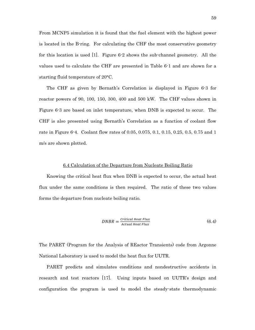
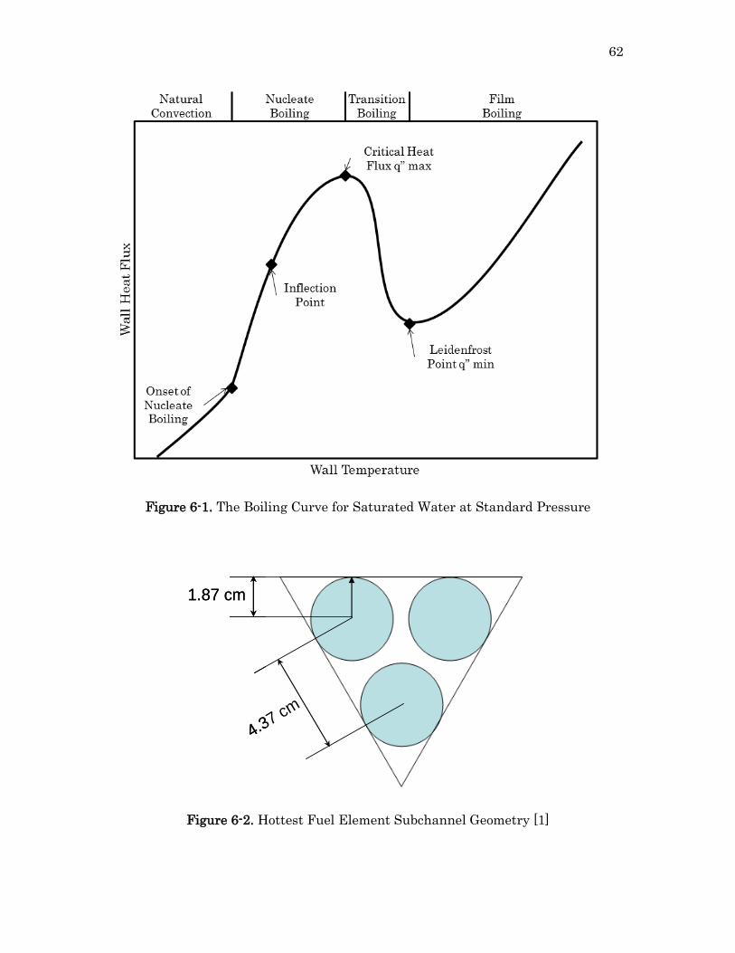
From MCNP5 simulation it is found that the fuel element with the highest power
is located in the B-ring. For calculating the CHF the most conservative geometry
for this location is used [1]. Figure 6-2 shows the sub-channel geometry. All the
values used to calculate the CHF are presented in Table 6-1 and are shown for a
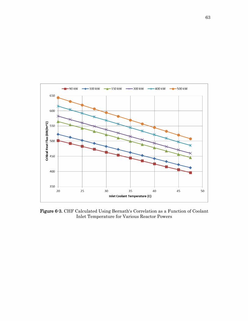
starting fluid temperature of 20°C.
The CHF as given by Bernath’s Correlation is displayed in Figure 6-3 for
reactor powers of 90, 100, 150, 300, 400 and 500 kW. The CHF values shown in
Figure 6-3 are based on inlet temperature, when DNB is expected to occur. The
CHF is also presented using Bernath’s Correlation as a function of coolant flow
rate in Figure 6-4. Coolant flow rates of 0.05, 0.075, 0.1, 0.15, 0.25, 0.5, 0.75 and 1
m/s are shown plotted.
6.4 Calculation of the Departure from Nucleate Boiling Ratio
Knowing the critical heat flux when DNB is expected to occur, the actual heat
flux under the same conditions is then required. The ratio of these two values
forms the departure from nucleate boiling ratio.
(6.4)
The PARET (Program for the Analysis of REactor Transients) code from Argonne
National Laboratory is used to model the heat flux for UUTR.
PARET predicts and simulates conditions and nondestructive accidents in
research and test reactors [17]. Using inputs based on UUTR’s design and
configuration the program is used to model the steady-state thermodynamic
60
conditions including coolant and fuel temperatures, and heat flux. These are
modeled for both the hottest and nominal fuel elements.
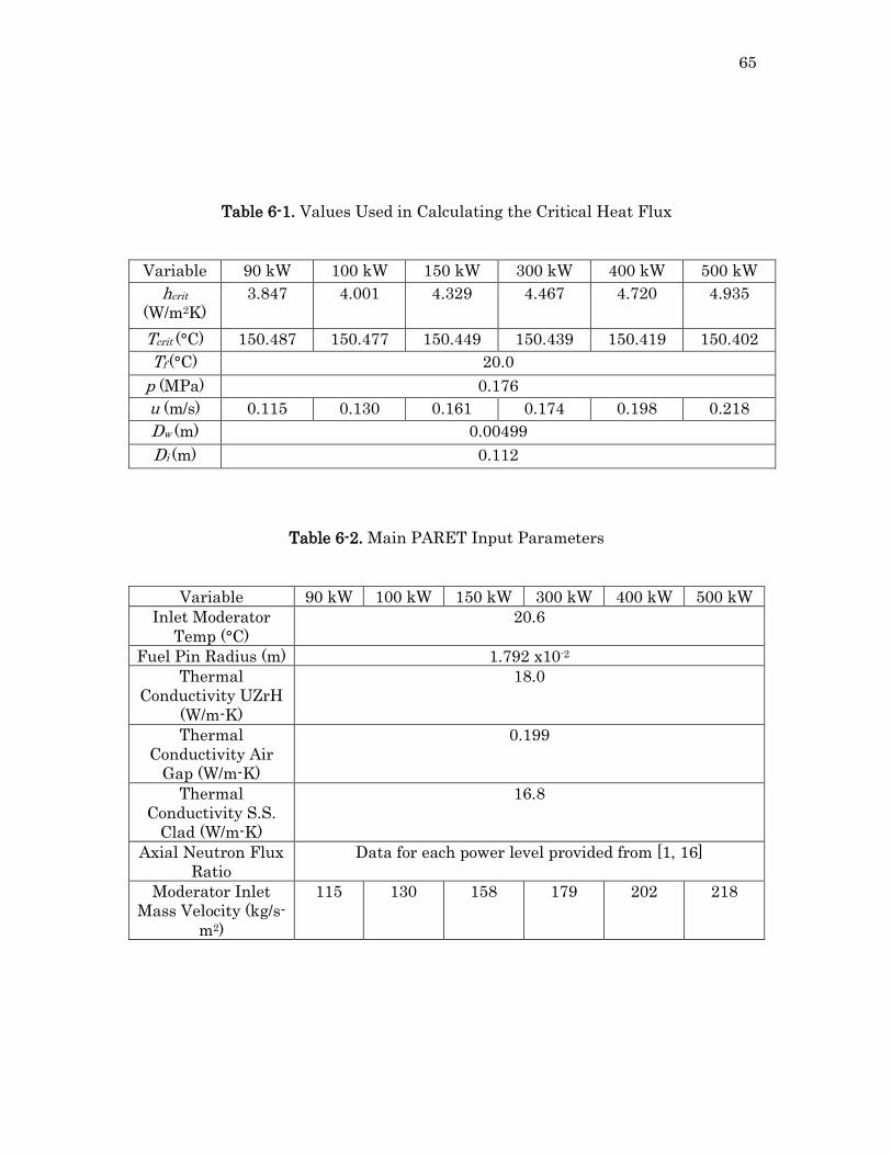
Table 6-2 shows the main input parameters used in the PARET code with the full
version of the code being included in Appendix D. The PARET code provides
information such as axial profiles of moderator temperature, fuel element
temperature and fuel element surface heat flux. Only the maximum surface heat
flux from the hottest fuel element is of interest for the DNBR calculation and is
shown in Table 6-3.
The CHF is read from the plots generated using Bernath’s Correlation in
Figure 6-3. The UUTR Technical Specifications require that the pool water
temperature be no higher than 35°C [1] so the CHF is read at this temperature by
finding the point at which each power level intersects the 35°C line. The resulting
critical heat fluxes and departure from nucleate boiling ratios are shown in Table
6-4.
6.5 UUTR Boiling Analysis
The DNBR calculation shows that using Bernath’s Correlation and maximum
heat flux data from the PARET code that a boiling crisis will not occur even if the
UUTR’s power is upgraded to 500 kW. Currently, during 90 kW operations there
is no boiling on any of the reactor fuel elements. Based only on the absolute
pressure at the bottom of the reactor tank the boiling point of the tank water would
be elevated to 127.5°C. PARET factors into account the coolant flow rate and
calculates a new temperature for the start of DNB. This is displayed for the
hottest fuel channel in Table 6-5 and is compared to the highest fuel cladding
surface temperature calculated.

61
The DNB temperature is a function of the coolant flow rate, increasing or
decreasing as the rate speeds up or slows down respectively. The coolant flow rate
is driven by the natural convection current and increases as the heat flux and
reactor power increase. However, the increase in the heat flux with higher reactor
powers outpaces the increase in the coolant flow rate leading to the cladding
surface temperature meeting the DNB temperature of 131.9°C when the reactor is
operating at 210 kW. After this point the boiling is still in a nucleate regime but
this shows that the inflection point shown on Figure 6-1 has been reached. The
500 kW PARET simulation shows that the boiling remains in this state and does
not increase above the CHF.
62
Figure 6-1. The Boiling Curve for Saturated Water at Standard Pressure
Figure 6-2. Hottest Fuel Element Subchannel Geometry [1]
4.37 cm
1.87 cm
4.37 cm
1.87 cm
63
Figure 6-3. CHF Calculated Using Bernath's Correlation as a Function of Coolant
Inlet Temperature for Various Reactor Powers

64
Figure 6-4. CHF Calculated Using Bernath's Correlation as a Function of Coolant
Inlet Temperature and Coolant Flow Rate
65
Table 6-1. Values Used in Calculating the Critical Heat Flux
Variable 90 kW 100 kW 150 kW 300 kW 400 kW 500 kW
hcrit
(W/m2K)
3.847 4.001 4.329 4.467 4.720 4.935
Tcrit (°C) 150.487 150.477 150.449 150.439 150.419 150.402
Tf (°C) 20.0
p (MPa) 0.176
u (m/s) 0.115 0.130 0.161 0.174 0.198 0.218
Dw (m) 0.00499
Di (m) 0.112
Table 6-2. Main PARET Input Parameters
Variable 90 kW 100 kW 150 kW 300 kW 400 kW 500 kW
Inlet Moderator
Temp (°C)
20.6
Fuel Pin Radius (m) 1.792 x10⁻²
Thermal
Conductivity UZrH
(W/m-K)
18.0
Thermal
Conductivity Air
Gap (W/m-K)
0.199
Thermal
Conductivity S.S.
Clad (W/m-K)
16.8
Axial Neutron Flux
Ratio
Data for each power level provided from [1, 16]
Moderator Inlet
Mass Velocity (kg/s-
m2)
115 130 158 179 202 218

66
Table 6-3. PARET Calculated Maximum Surface Heat Flux
UUTR Power Level Maximum Heat Flux (W/m2)
90 kW 44,419
100 kW 49,057
150 kW 74,032
300 kW 148,064
400 kW 197,419
500 kW 246,774
Table 6-4. UUTR Critical Heat Flux and DNBR at 35°C
Power Level Critical Heat Flux (kW/m2) DNBR
90 kW 444.2 10.00
100 kW 462.5 9.43
150 kW 499.8 6.75
300 kW 515.6 3.48
400 kW 544.7 2.76
500 kW 569.5 2.31
Table 6-5. PARET Hottest Element Calculated DNB and Cladding Surface
Temperatures
Power Level DNB Temperature
(°C)
Cladding Surface
Temperature (°C)
90 kW 130.93 100.88
100 kW 131.25 101.45
150 kW 131.77 124.00
300 kW 132.10 133.43
400 kW 132.44 134.80
500 kW 132.66 135.93
67
CHAPTER 7
HIGHER POWER UUTR COOLING SYSTEM DESIGN
7.1 Introduction
Extended operations of the UUTR at higher power levels necessitate the need
of a new cooling system. Similar upgrades and costs are investigated at other
research facilities [21, 22, 23 and 24]. For the UUTR two systems are proposed: a
low-cost component upgrade and a complete new design. Costs, materials and the
benefits of both proposals are compared.
7.2 Review of the Upgrades at Other Facilities
Reactor modernization and refurbishment is not uncommon among research
reactors and often includes upgrades increases to the power and cooling system
[21]. TRIGA reactor upgrades in Brazil, Indonesia and at Oregon State University
are analyzed for their upgrades and described in brief as follows.
The IPR-R1 TRIGA Mark I reactor in Belo Horizonte, Brazil was upgraded
from 30 kW to 250 kW in 1970 [22]. This system was most similar to UUTR
because of the presence of a 30 kW refrigeration cooling system attached to the
water purification loop. The purification loop was kept in place for use in the new
system. All piping was replaced with stainless steel and underground conduits
were dug for piping connections to the outside cooling tower. The heat exchanger

68
was a shell and tube type designed for an input temperature of 40.7°C and an
output of 33.1°C with a mass flow rate of 30,000 kg/hr. The cooling tower was
designed for a wet bulb temperature of 24.4°C and a flow rate of 40,000 kg/hr.
Installation was done in parallel with reactor operations with a maximum
shutdown time of two days. Total costs were calculated to be $225,000 (in 2012
dollars) [22].
The Bandung TRIGA Mark II reactor in Bandung, Indonesia completed a power
and cooling system upgrade from 1,000 kW to 2,000 kW in the year 2000 [23].
During the retrofit nearly all reactor components were upgraded including: the
core, a new tank and a new primary and secondary cooling system. The new
system was built with a plate type heat exchanger connected to two cooling towers
located outside. Both were rated to 2,400 kW of cooling load and were designed
and built locally by the Nuclear Technology Center. One million dollars was
budgeted for the design, construction and building of the new cooling, ventilation
and I & C systems. The complete upgrade took four years to finish.
The Oregon State TRIGA reactor in Corvallis, Oregon has also undergone a
similar upgrade [24]. In 1970 the reactor was upgraded from 250 kW to 1 MW. A
1 MW shell and tube heat exchanger linked to a cooling tower was installed over
seven months in 1971. A new coolant flow rate of 350 gpm was measured. Some
observations were made after the installation: radiation levels decreased on the top
of the reactor tank by two to three times, a low resonance vibration can sometimes
be detected in the core and radiation levels in the demineralizer have increased
eight times. It is believed that the radiation level decrease is due to the higher
flow rate allowing less N-16 to reach the surface while the higher level is caused by
increased sediment from the bottom of the tank getting picked up and trapped in
69
the demineralizer. The vibration detected was found to be caused by nucleate
boiling taking place on the fuel elements.
7.3 UUTR Low-Cost Upgrade
Without any core or reactor modifications it is found that the maximum UUTR
power level is 150 kW [16]. UUTR does not operate at this level as only two hours
and six minutes of runtime would be available if started at 20°C before the internal
temperature limit of 30°C would be reached. This limit is set to avoid the
Technical Specifications limit of 35°C that protects the integrity of the deionizing
resin beds. At higher temperatures the resin integrity begins to degrade leaching
the removed contaminates back into the water.
Recently, higher grade, more temperature resistant deionizing resins have
become widely available for less cost. Manufacturers such as ResinTech® and
Purolite® both make products that fit in this category [25, 26]. The ResinTech®
MBD-10 nuclear grade, mixed bed resin functions up to 60°C if rechargeable and
up to 80°C if single use and meets all other water quality requirements [27]. In a
telephone interview conducted with a local water equipment supplier the cost of a
new, higher grade deionizing resin was estimated at $3,000-$5,000 and could be
installed with minimal effort [28].
To extend the operating time and increase the operating power of UUTR for
minimal cost it is recommended that one of these new deionizing beds be installed
and the Technical Specifications be amended to have a water temperature limit of
45°C. Operating under these conditions the new internal temperature limit would
be set at 40°C. This increase in temperature limit would allow three and a half
additional hours of operating time at 90 kW or two hours and ten minutes
70
additional time if upgraded and operating at 150 kW. Figure 7-1, based off of the
previous simulations conducted, illustrates the theoretical runtimes for various
power levels when starting at 20°C.
This upgrade only retrofits UUTR for higher temperature operations and does
not provide any additional cooling capabilities. UUTR would still be cooled
through natural heat transfer to the surroundings. Because of this extra shutdown
time would be required following higher temperature runs to allow for ambient
cooling. Based on the current schedule of UUTR activity with two to three runs
per month this should not be an issue.
7.4 UUTR Complete Cooling System Replacement
To enable longer, more frequent UUTR runtimes with an increase in power
level a new cooling system needs to be considered. A dual-loop system connected
through a heat exchanger and routed to an outdoor cooling tower is commonly used
to cool research reactors and would be best suited for UUTR. A basic piping and
instrumentation diagram for a theoretical UUTR system is shown in Figure 7-2.
For the sole purpose of estimating the costs of a cooling system UUTR is
assumed to be operating at 250 kW and the system components are sized
appropriately. The theoretical layout in Figure 7-2 would suit any higher power
core. Only the size of the heat exchanger, cooling tower, pumps and pipes change
as needed. Assuming a 20°C temperature difference in the cooling water from the
heat exchanger, a flow rate of 47.4 gpm is required to cool a 250 kW reactor. This
assumes no flow losses and is illustrated for other power levels in Figure 7-3.
To supply this flow rate and provide extra head for the losses occurring in the
pipes, resin beds and heat exchanger a 5 hp pump is needed costing about $1,500.
71
These pumps commonly use 2.5 or 3 inch piping connections. Stainless steel,
schedule 40 pipe is strong, durable and well suited to this type of operation. It is
estimated that 60 feet of piping and fittings are needed for the primary loop and is
estimated at $3,000 (use of aluminum piping would be less) [29].
The heat exchanger connects both sides of the cooling loop and is the most
important piece in the system. These components are typically manufactured to
meet the heat transfer needs of the reactor. Two companies, Alfa Laval and
Graham, have experience making heat exchangers for research reactors. In a
conversation with the manufacturer it is recommended that a plate heat exchanger
be used and would cost approximately $20,000 [30].
The secondary loop supplies cooled water to the heat exchanger from the
cooling tower. Because of Utah’s dry climate an open circuit cooling tower is the
more efficient choice. A 300 kW counter-flow cooling tower is recommended as it
allows for maximum heat transfer from the heat exchanger, has a more freeze
resistant design for winter use and is commonly available in preassembled units.
From conversations with a manufacturer, units of this type are available for
$25,000 with about $25,000 more needed to complete the installation [31].
As in the primary loop, the secondary loop also requires a pump and piping
network. If the cooling tower is located near the outside wall of the UNEP facility
approximately 30 feet of piping would be needed for a cost of $2,000. The cooling
tower requires a maximum of 110 gpm of water flow. With the reduced head
needed a pump similar to the one in the primary loop can be used for a cost of
$1,500. Because the cooling tower is open to the atmosphere, a water treatment
system is recommended for the secondary loop to prevent fouling. The
manufacturer of the cooling tower says these systems range around $5,000 [31].
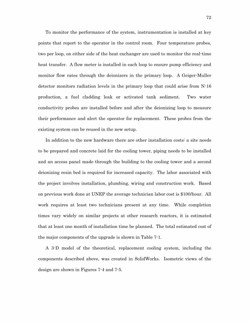
72
To monitor the performance of the system, instrumentation is installed at key
points that report to the operator in the control room. Four temperature probes,
two per loop, on either side of the heat exchanger are used to monitor the real-time
heat transfer. A flow meter is installed in each loop to ensure pump efficiency and
monitor flow rates through the deionizers in the primary loop. A Geiger-Muller
detector monitors radiation levels in the primary loop that could arise from N-16
production, a fuel cladding leak or activated tank sediment. Two water
conductivity probes are installed before and after the deionizing loop to measure
their performance and alert the operator for replacement. These probes from the
existing system can be reused in the new setup.
In addition to the new hardware there are other installation costs: a site needs
to be prepared and concrete laid for the cooling tower, piping needs to be installed
and an access panel made through the building to the cooling tower and a second
deionizing resin bed is required for increased capacity. The labor associated with
the project involves installation, plumbing, wiring and construction work. Based
on previous work done at UNEP the average technician labor cost is $100/hour. All
work requires at least two technicians present at any time. While completion
times vary widely on similar projects at other research reactors, it is estimated
that at least one month of installation time be planned. The total estimated cost of
the major components of the upgrade is shown in Table 7-1.
A 3-D model of the theoretical, replacement cooling system, including the
components described above, was created in SolidWorks. Isometric views of the
design are shown in Figures 7-4 and 7-5.
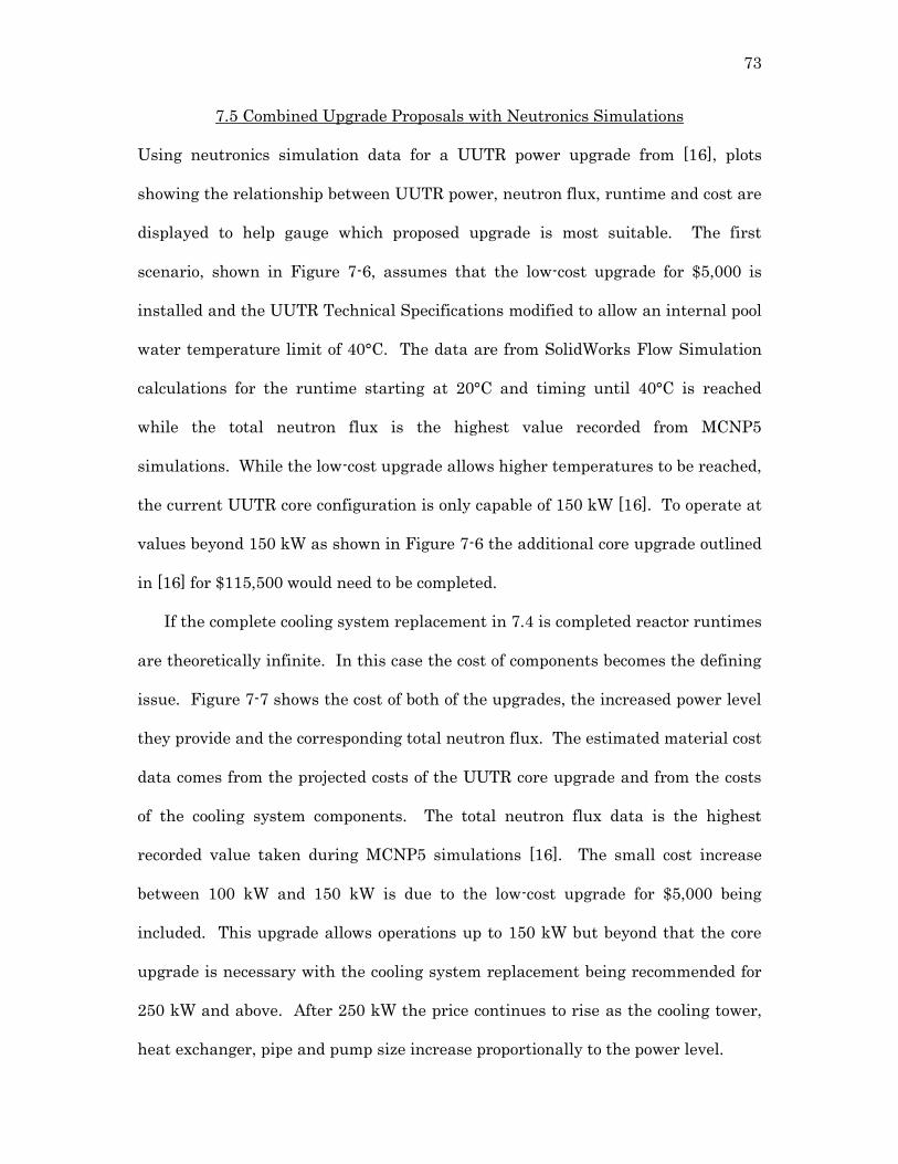
73
7.5 Combined Upgrade Proposals with Neutronics Simulations
Using neutronics simulation data for a UUTR power upgrade from [16], plots
showing the relationship between UUTR power, neutron flux, runtime and cost are
displayed to help gauge which proposed upgrade is most suitable. The first
scenario, shown in Figure 7-6, assumes that the low-cost upgrade for $5,000 is
installed and the UUTR Technical Specifications modified to allow an internal pool
water temperature limit of 40°C. The data are from SolidWorks Flow Simulation
calculations for the runtime starting at 20°C and timing until 40°C is reached
while the total neutron flux is the highest value recorded from MCNP5
simulations. While the low-cost upgrade allows higher temperatures to be reached,
the current UUTR core configuration is only capable of 150 kW [16]. To operate at
values beyond 150 kW as shown in Figure 7-6 the additional core upgrade outlined
in [16] for $115,500 would need to be completed.
If the complete cooling system replacement in 7.4 is completed reactor runtimes
are theoretically infinite. In this case the cost of components becomes the defining
issue. Figure 7-7 shows the cost of both of the upgrades, the increased power level
they provide and the corresponding total neutron flux. The estimated material cost
data comes from the projected costs of the UUTR core upgrade and from the costs
of the cooling system components. The total neutron flux data is the highest
recorded value taken during MCNP5 simulations [16]. The small cost increase
between 100 kW and 150 kW is due to the low-cost upgrade for $5,000 being
included. This upgrade allows operations up to 150 kW but beyond that the core
upgrade is necessary with the cooling system replacement being recommended for
250 kW and above. After 250 kW the price continues to rise as the cooling tower,
heat exchanger, pipe and pump size increase proportionally to the power level.

74
Figure 7-1. UUTR Pool Water Temperature as a Function of UUTR Power after TS
Temperature Increase as Obtained with SolidWorks Flow Simulation

75
Figure 7-2. Theoritical UUTR Upgraded Cooling System Design
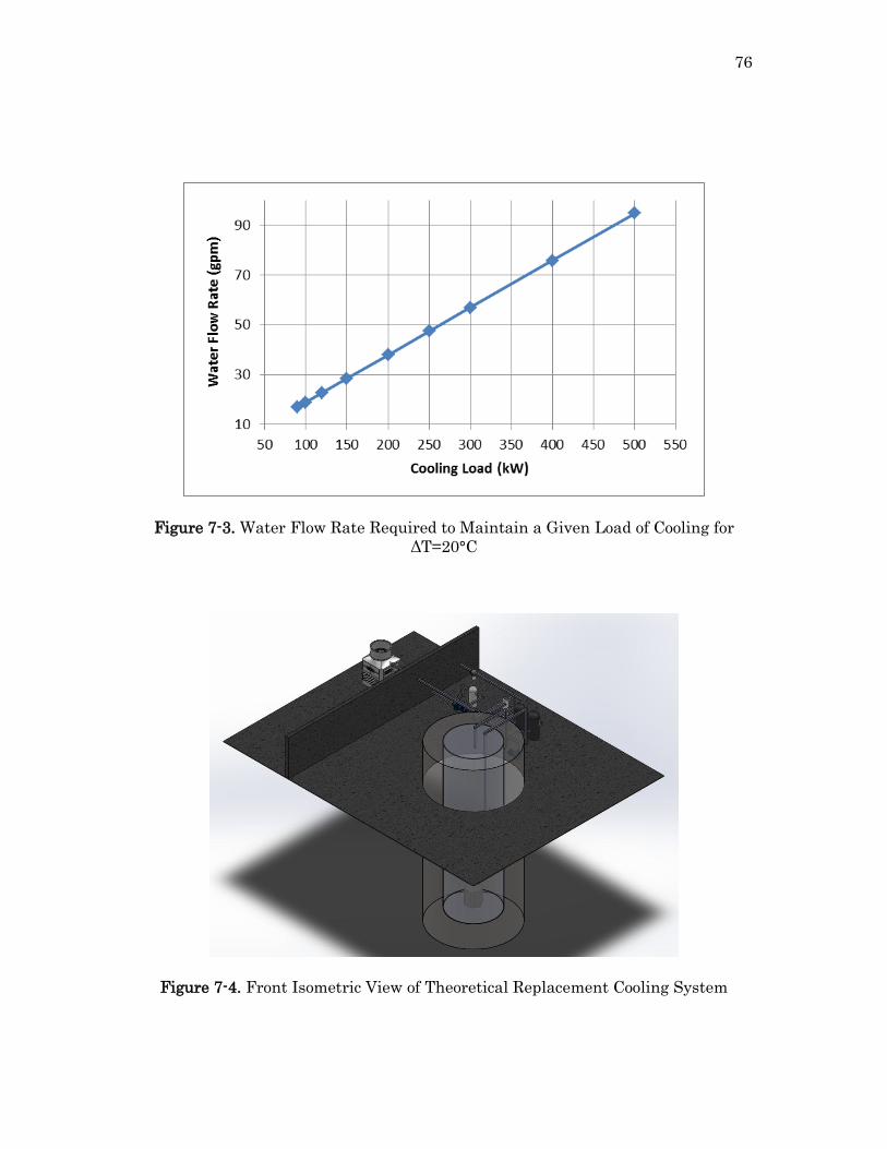
76
Figure 7-3. Water Flow Rate Required to Maintain a Given Load of Cooling for
ΔT=20°C
Figure 7-4. Front Isometric View of Theoretical Replacement Cooling System
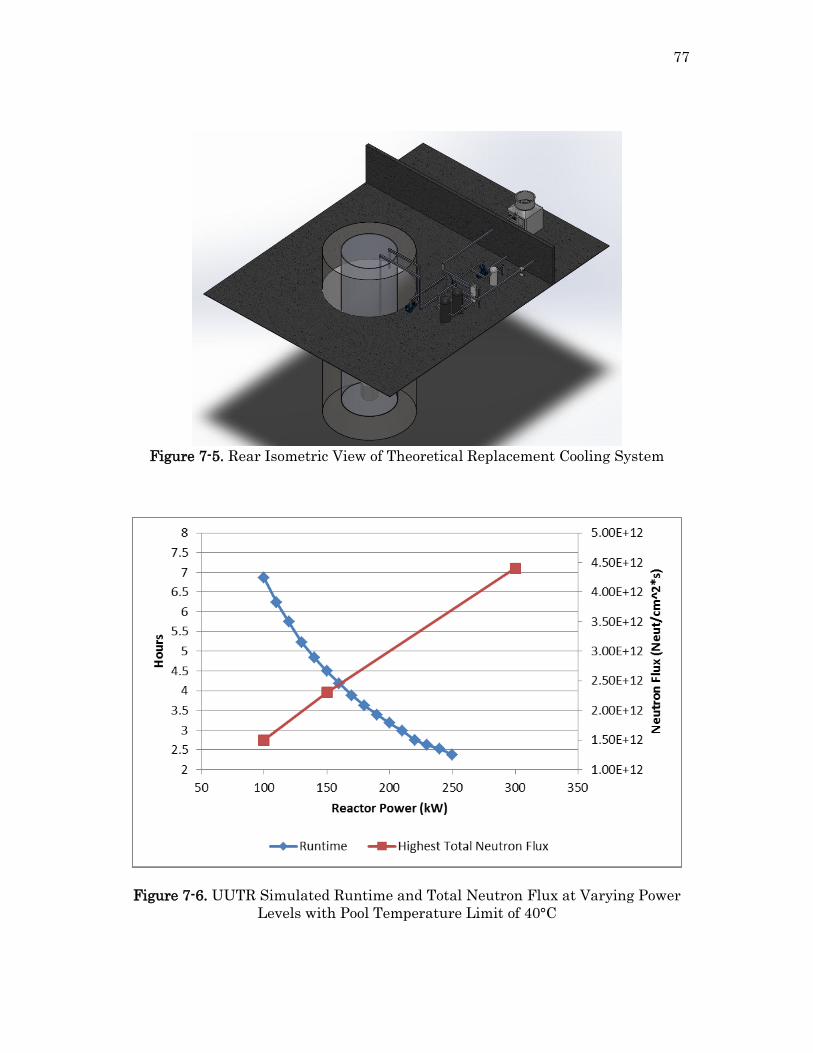
77
Figure 7-5. Rear Isometric View of Theoretical Replacement Cooling System
Figure 7-6. UUTR Simulated Runtime and Total Neutron Flux at Varying Power
Levels with Pool Temperature Limit of 40°C
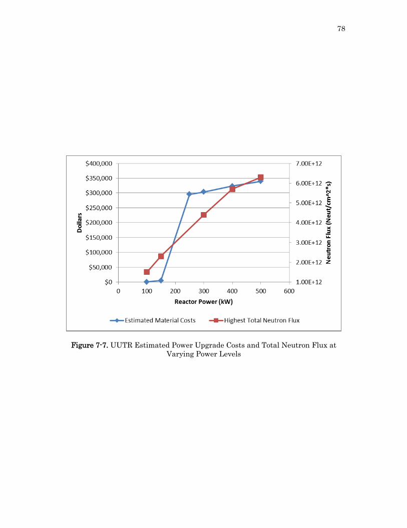
78
Figure 7-7. UUTR Estimated Power Upgrade Costs and Total Neutron Flux at
Varying Power Levels
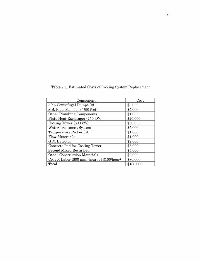
79
Table 7-1. Estimated Costs of Cooling System Replacement
Component Cost
5 hp Centrifugal Pumps (2) $3,000
S.S. Pipe, Sch. 40, 3” (90 feet) $5,000
Other Plumbing Components $1,000
Plate Heat Exchanger (250 kW) $20,000
Cooling Tower (300 kW) $50,000
Water Treatment System $5,000
Temperature Probes (4) $1,000
Flow Meters (2) $1,000
G-M Detector $2,000
Concrete Pad for Cooling Tower $5,000
Second Mixed Resin Bed $5,000
Other Construction Materials $2,000
Cost of Labor (800 man-hours @ $100/hour) $80,000
Total $180,000

80
CHAPTER 8
CONCLUSION AND FUTURE WORK
8.1 Conclusion
The objectives of this thesis were to analyze the thermohydraulics aspects of
increasing UUTR’s power and determine a design basis area for this upgrade with
a cost estimate. This was done by first conducting a survey of research reactors
and their cooling systems. Simulations of reactor pool conditions were completed
using SolidWorks Flow Simulation and Ansys Fluent. 3-D models of the UUTR
core and pool were created in each with the flow conditions and temperatures being
simulated. An analysis of the departure from nucleate boiling in UUTR was
carried out using the PARET-ANL code. The results from these simulations form a
basis for a power upgrade to UUTR. Based on these results two potential upgrades
were proposed: a low cost upgrade for extended operations was quoted for $5,000
while materials for a complete system replacement that would allow continuous
reactor operations were estimated starting at $180,000.
8.2 Recommendations for Future Work
The simulations in Flow Works and Fluent provide insight into UUTR pool
conditions at higher powers. These models include the entire reactor pool with a
simpler version of the core. The next step using these simulations would be a
81
higher detail model of the UUTR core without including the surrounding pool.
This would allow each individual fuel channel to be modeled and the flow through
each to be simulated. These results could then be compared to the hot and nominal
channel results from the PARET-ANL code. This would help more accurately
determine the DNBR and plan for an ideal future higher power for UUTR.
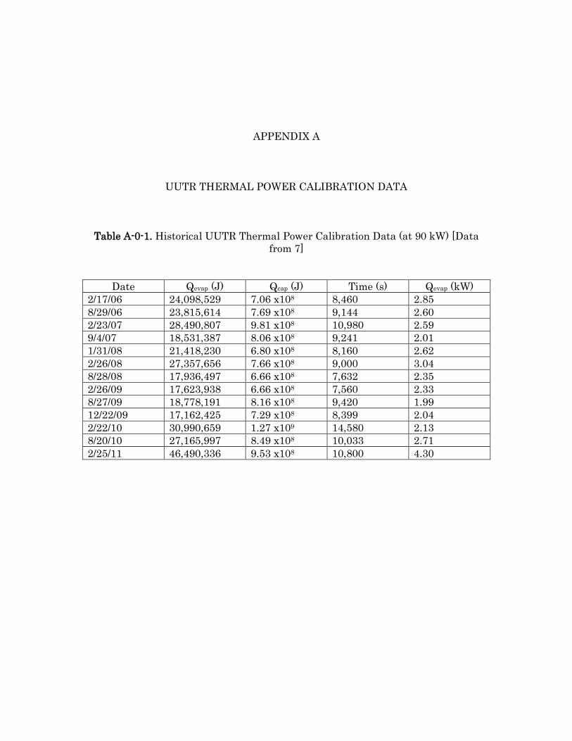
82
APPENDIX A
UUTR THERMAL POWER CALIBRATION DATA
Table A-0-1. Historical UUTR Thermal Power Calibration Data (at 90 kW) [Data
from 7]
Date Qevap (J) Qcap (J) Time (s) Qevap (kW)
2/17/06 24,098,529 7.06 x10⁸ 8,460 2.85
8/29/06 23,815,614 7.69 x10⁸ 9,144 2.60
2/23/07 28,490,807 9.81 x10⁸ 10,980 2.59
9/4/07 18,531,387 8.06 x10⁸ 9,241 2.01
1/31/08 21,418,230 6.80 x10⁸ 8,160 2.62
2/26/08 27,357,656 7.66 x10⁸ 9,000 3.04
8/28/08 17,936,497 6.66 x10⁸ 7,632 2.35
2/26/09 17,623,938 6.66 x10⁸ 7,560 2.33
8/27/09 18,778,191 8.16 x10⁸ 9,420 1.99
12/22/09 17,162,425 7.29 x10⁸ 8,399 2.04
2/22/10 30,990,659 1.27 x10⁹ 14,580 2.13
8/20/10 27,165,997 8.49 x10⁸ 10,033 2.71
2/25/11 46,490,336 9.53 x10⁸ 10,800 4.30
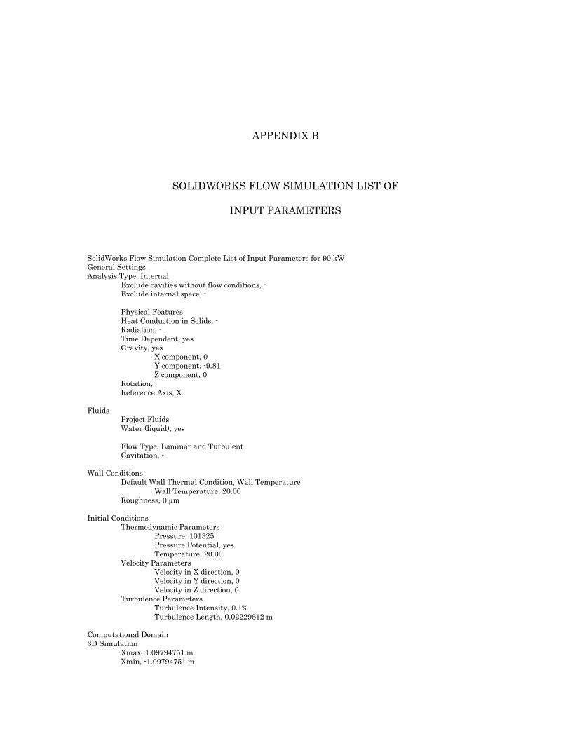
83
APPENDIX B
SOLIDWORKS FLOW SIMULATION LIST OF
INPUT PARAMETERS
SolidWorks Flow Simulation Complete List of Input Parameters for 90 kW
General Settings
Analysis Type, Internal
Exclude cavities without flow conditions, -
Exclude internal space, -
Physical Features
Heat Conduction in Solids, -
Radiation, -
Time Dependent, yes
Gravity, yes
X component, 0
Y component, -9.81
Z component, 0
Rotation, -
Reference Axis, X
Fluids
Project Fluids
Water (liquid), yes
Flow Type, Laminar and Turbulent
Cavitation, -
Wall Conditions
Default Wall Thermal Condition, Wall Temperature
Wall Temperature, 20.00
Roughness, 0 µm
Initial Conditions
Thermodynamic Parameters
Pressure, 101325
Pressure Potential, yes
Temperature, 20.00
Velocity Parameters
Velocity in X direction, 0
Velocity in Y direction, 0
Velocity in Z direction, 0
Turbulence Parameters
Turbulence Intensity, 0.1%
Turbulence Length, 0.02229612 m
Computational Domain
3D Simulation
Xmax, 1.09794751 m
Xmin, -1.09794751 m
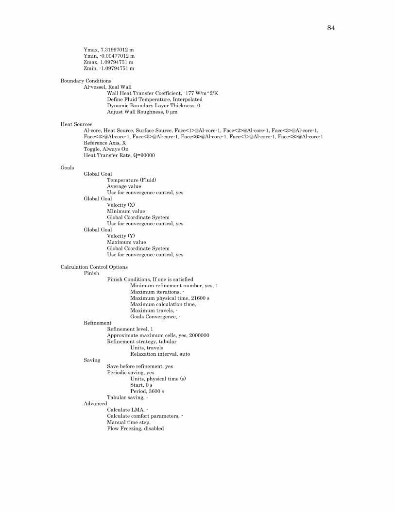
84
Ymax, 7.31997012 m
Ymin, -0.00477012 m
Zmax, 1.09794751 m
Zmin, -1.09794751 m
Boundary Conditions
Al-vessel, Real Wall
Wall Heat Transfer Coefficient, -177 W/m^2/K
Define Fluid Temperature, Interpolated
Dynamic Boundary Layer Thickness, 0
Adjust Wall Roughness, 0 µm
Heat Sources
Al-core, Heat Source, Surface Source, Face<1>@Al-core-1, Face<2>@Al-core-1, Face<3>@Al-core-1,
Face<4>@Al-core-1, Face<5>@Al-core-1, Face<6>@Al-core-1, Face<7>@Al-core-1, Face<8>@Al-core-1
Reference Axis, X
Toggle, Always On
Heat Transfer Rate, Q=90000
Goals
Global Goal
Temperature (Fluid)
Average value
Use for convergence control, yes
Global Goal
Velocity (X)
Minimum value
Global Coordinate System
Use for convergence control, yes
Global Goal
Velocity (Y)
Maximum value
Global Coordinate System
Use for convergence control, yes
Calculation Control Options
Finish
Finish Conditions, If one is satisfied
Minimum refinement number, yes, 1
Maximum iterations, -
Maximum physical time, 21600 s
Maximum calculation time, -
Maximum travels, -
Goals Convergence, -
Refinement
Refinement level, 1
Approximate maximum cells, yes, 2000000
Refinement strategy, tabular
Units, travels
Relaxation interval, auto
Saving
Save before refinement, yes
Periodic saving, yes
Units, physical time (s)
Start, 0 s
Period, 3600 s
Tabular saving, -
Advanced
Calculate LMA, -
Calculate comfort parameters, -
Manual time step, -
Flow Freezing, disabled

85
APPENDIX C
FLUENT SIMULATION LIST OF INPUT
PARAMETERS AND SETTINGS
*Fluent UUTR 250 kW (steady state) Thermohydraulic Simulation*
*Philip Babitz*
Check Mesh
General
Solver
Type; Pressure-Based
Velocity Formulation; Absolute
Time; Transient
Gravity; Enabled
Gravitational Acceleration
X; 0
Y; -9.81
Z; 0
Models
Multiphase; off
Energy; on
Viscous; laminar
Radiation; off
Heat Exchanger; off
Species; off
Discrete Phase; off
Solidification and Melting; off
Acoustics; off
Materials
Fluid; Water-liquid
Properties
Density; boussinesq, 998.2
Cp; constant, 4183
Thermal Conductivity; constant, 0.6
Viscosity, constant; 0.001003
Thermal Expansion Coefficient; constant, 0.000207
Solid; aluminum
Properties
Density; constant, 2719
Cp; constant, 871
Thermal Conductivity; constant, 202.4
Cell Zone Conditions
water-liquid
Type; fluid
ID; 2
Material name; water-liquid
Porous zone; off
Source terms; off
Fixed valus; off
Motion Type; stationary
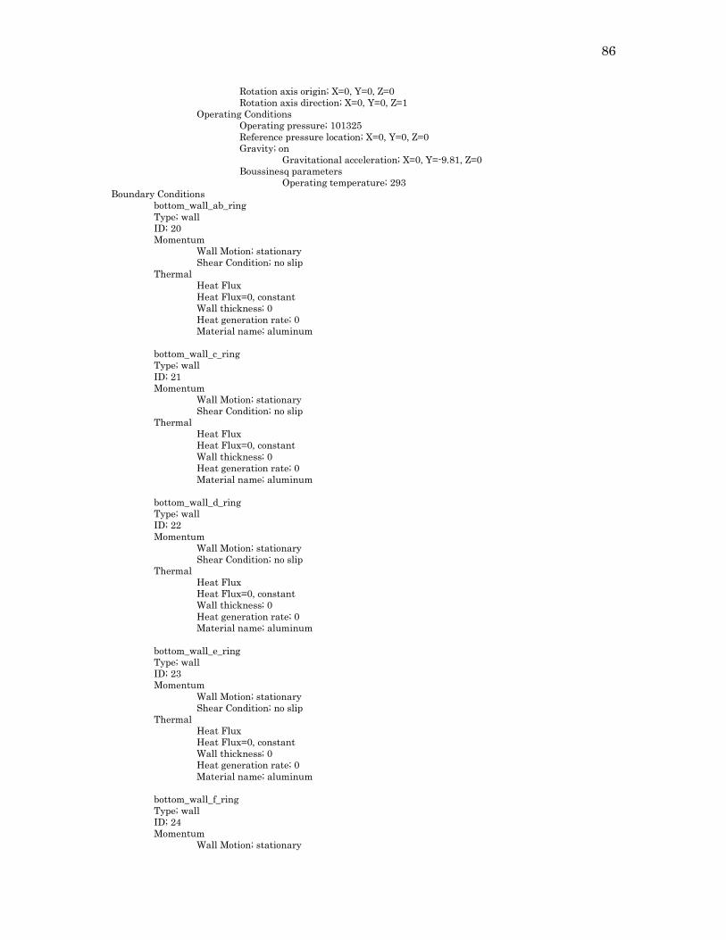
86
Rotation axis origin; X=0, Y=0, Z=0
Rotation axis direction; X=0, Y=0, Z=1
Operating Conditions
Operating pressure; 101325
Reference pressure location; X=0, Y=0, Z=0
Gravity; on
Gravitational acceleration; X=0, Y=-9.81, Z=0
Boussinesq parameters
Operating temperature; 293
Boundary Conditions
bottom_wall_ab_ring
Type; wall
ID; 20
Momentum
Wall Motion; stationary
Shear Condition; no slip
Thermal
Heat Flux
Heat Flux=0, constant
Wall thickness; 0
Heat generation rate; 0
Material name; aluminum
bottom_wall_c_ring
Type; wall
ID; 21
Momentum
Wall Motion; stationary
Shear Condition; no slip
Thermal
Heat Flux
Heat Flux=0, constant
Wall thickness; 0
Heat generation rate; 0
Material name; aluminum
bottom_wall_d_ring
Type; wall
ID; 22
Momentum
Wall Motion; stationary
Shear Condition; no slip
Thermal
Heat Flux
Heat Flux=0, constant
Wall thickness; 0
Heat generation rate; 0
Material name; aluminum
bottom_wall_e_ring
Type; wall
ID; 23
Momentum
Wall Motion; stationary
Shear Condition; no slip
Thermal
Heat Flux
Heat Flux=0, constant
Wall thickness; 0
Heat generation rate; 0
Material name; aluminum
bottom_wall_f_ring
Type; wall
ID; 24
Momentum
Wall Motion; stationary
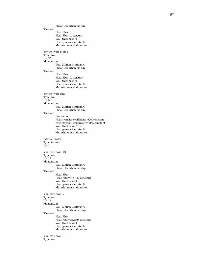
87
Shear Condition; no slip
Thermal
Heat Flux
Heat Flux=0, constant
Wall thickness; 0
Heat generation rate; 0
Material name; aluminum
bottom_wall_g_ring
Type; wall
ID; 25
Momentum
Wall Motion; stationary
Shear Condition; no slip
Thermal
Heat Flux
Heat Flux=0, constant
Wall thickness; 0
Heat generation rate; 0
Material name; aluminum
bottom_wall_ring
Type; wall
ID; 5
Momentum
Wall Motion; stationary
Shear Condition; no slip
Thermal
Convection
Heat transfer coefficient=920, constant
Free stream temperature=295, constant
Wall thickness; .75 in
Heat generation rate; 0
Material name; aluminum
interior_water
Type; interior
ID; 1
side_core_wall_10
Type; wall
ID; 19
Momentum
Wall Motion; stationary
Shear Condition; no slip
Thermal
Heat Flux
Heat Flux=375138, constant
Wall thickness; 0
Heat generation rate; 0
Material name; aluminum
side_core_wall_2
Type; wall
ID; 14
Momentum
Wall Motion; stationary
Shear Condition; no slip
Thermal
Heat Flux
Heat Flux=287880, constant
Wall thickness; 0
Heat generation rate; 0
Material name; aluminum
side_core_wall_3
Type; wall

88
ID; 15
Momentum
Wall Motion; stationary
Shear Condition; no slip
Thermal
Heat Flux
Heat Flux=279673, constant
Wall thickness; 0
Heat generation rate; 0
Material name; aluminum
side_core_wall_5
Type; wall
ID; 16
Momentum
Wall Motion; stationary
Shear Condition; no slip
Thermal
Heat Flux
Heat Flux=344649, constant
Wall thickness; 0
Heat generation rate; 0
Material name; aluminum
side_core_wall_7
Type; wall
ID; 17
Momentum
Wall Motion; stationary
Shear Condition; no slip
Thermal
Heat Flux
Heat Flux=379616, constant
Wall thickness; 0
Heat generation rate; 0
Material name; aluminum
side_core_wall_9
Type; wall
ID; 18
Momentum
Wall Motion; stationary
Shear Condition; no slip
Thermal
Heat Flux
Heat Flux=513023, constant
Wall thickness; 0
Heat generation rate; 0
Material name; aluminum
side_water_wall
Type; wall
ID; 6
Momentum
Wall Motion; stationary
Shear Condition; no slip
Thermal
Convection
Heat transfer coefficient=920, constant
Free stream temperature=295, constant
Wall thickness; .75 in
Heat generation rate; 0
Material name; aluminum
top_wall_ab_ring
Type; wall
ID; 8

89
Momentum
Wall Motion; stationary
Shear Condition; no slip
Thermal
Heat Flux
Heat Flux=427421, constant
Wall thickness; 0
Heat generation rate; 0
Material name; aluminum
top_wall_c_ring
Type; wall
ID; 9
Momentum
Wall Motion; stationary
Shear Condition; no slip
Thermal
Heat Flux
Heat Flux=387723, constant
Wall thickness; 0
Heat generation rate; 0
Material name; aluminum
top_wall_d_ring
Type; wall
ID; 10
Momentum
Wall Motion; stationary
Shear Condition; no slip
Thermal
Heat Flux
Heat Flux=290095, constant
Wall thickness; 0
Heat generation rate; 0
Material name; aluminum
top_wall_e_ring
Type; wall
ID; 11
Momentum
Wall Motion; stationary
Shear Condition; no slip
Thermal
Heat Flux
Heat Flux=291515, constant
Wall thickness; 0
Heat generation rate; 0
Material name; aluminum
top_wall_f_ring
Type; wall
ID; 12
Momentum
Wall Motion; stationary
Shear Condition; no slip
Thermal
Heat Flux
Heat Flux=202471, constant
Wall thickness; 0
Heat generation rate; 0
Material name; aluminum
top_wall_g_ring
Type; wall
ID; 13
Momentum
Wall Motion; stationary
90
Shear Condition; no slip
Thermal
Heat Flux
Heat Flux=25275, constant
Wall thickness; 0
Heat generation rate; 0
Material name; aluminum
top_water_wall
Type; wall
ID; 7
Momentum
Wall Motion; stationary
Shear Condition; no slip
Thermal
Convection
Heat transfer coefficient=0, constant
Free stream temperature=295, constant
Wall thickness; 0
Heat generation rate; 0
Material name; aluminum
Dynamic Mesh; off
Reference Values
Area; 1
Density; 1.225
Enthalpy; 0
Length; 39.37008
Pressure; 0
Temperature; 288.16
Velocity; 1
Viscosity; 1.7894e-05
Ratio of specific heats; 1.4
Reference zone; water
Solution Methods
Scheme; PISO
Skewness correction; 1
Neighbor correction; 1
Skewness-neighbor coupling; on
Spatial Discretization
Gradient; least squares cell based
Pressure; second order
Momentum; first order upwind
Energy; first order upwind
Transient Formulation; first order implicit
Non-iterative time advancement; off
Frozen flux formulation; off
Solution Controls
Under-relaxation Factors
Pressure; 0.3
Density; 1
Body forces; 1
Momentum; 0.7
Energy; 1
Monitors
Residuals; print, plot
Statistic; off
Drag; off
Lift; off
Moment; off
Solution Initialization
Reference Frame; relative to cell zone
91
Initial Values
Gauge Pressure; 0
X velocity; 0.002
Y velocity; 0.01
Z velocity; 0.002
Temperature; 293
Calculation Activities
Autosave timesteps; 300
Solution animations; 2
Temp; 300, s, x-center
Vel; 300, s, x-center
Run Calculation
Time step; fixed
Time step size; 1
Number of time steps; 3600
Max iterations/time step; 700
Reporting interval; 10
Profile update interval; 10
Calculate

92
APPENDIX D
PARET-ANL INPUT CODE
*PARET: The University of Utah TRIGA Reactor: 150kW (Steady State)
1001, -2 19 7 1 0 1
1002, 0 0 6 -1 0 20
1003, 1.5-1 0.032540 1.66339+5 -20.60 1.79200-2
1004, 1.74110-2 1.74200-2 0.0 0.0 0.3810 0.1016
1005, 0.1016 0.0078 27.900-6 9.80664 0.00679
1006 0.00 0.80 1.0 998.63 -0.47296
1007, -2.02010-3 1.15817-5 0.00 0.00 1.00 0.001
1008, 0.00 0.001 0.001 0.05 0.05 0.05
1009, 1.4 0.33
1111, 0.039556 1.00 1.00
1112, 0 1 1 6 1 0
1113, 3.81 0.2 10000.0 0.00
1114, 6.7056 0.6096
2001, 0.0 0.0 18.00 0.00 0.00
2002, 0.0 0.4170+4 2.0400+6 0.00 -273.0
2003, 0.0 0.0 0.199000 0.00 0.00
2004, 0.0 0.0 6.66340+2 0.00 0.00
2005, 0.0 0.0 16.8 0.00 0.00
2006, 0.0 0.0 3.975+6 0.00 0.00
3001, 4.35275-3 5 1 0.980
3002, 9.0-6 6 2 0.000
3003, 5.00-4 7 3 0.000
4001, 0.02005 19
5100, 1 0 0.02794 0.007874 0.5 0.55 1.0
5100, 1.00 0.00 0.00
5101, 0.6096 6.7056 4.38511-2 4.38511-2 1.3818 1.250
5102 1.0988 1.00 1.00 1.00
5103, 1.1244 1.00 1.00 1.00
5104, 1.2662 1.00 1.00 1.00
5105, 1.4256 1.00 1.00 1.00
5106, 1.5657 1.00 1.00 1.00
5107, 1.6921 1.00 1.00 1.00
5108, 1.7812 1.00 1.00 1.00
5109, 1.8524 1.00 1.00 1.00
5110, 1.8965 1.00 1.00 1.00
5111, 1.9373 1.00 1.00 1.00
5112, 1.8960 1.00 1.00 1.00
5113, 1.8515 1.00 1.00 1.00
5114, 1.7789 1.00 1.00 1.00
5115, 1.6881 1.00 1.00 1.00
5116, 1.5595 1.00 1.00 1.00
5117, 1.4162 1.00 1.00 1.00
5118, 1.2536 1.00 1.00 1.00
5119, 1.1078 1.00 1.00 1.00
5120, 1.0797 1.00 1.00 1.00
5200, 1 0 0.02794 0.992126 0.5 0.55 1.00
5200, 1.00 0.0 0.0
5201, 0.6096 6.7056 4.38511-2 4.38511-2 1.3818 1.250
93
5202, 0.8326 1.00 1.00 1.00
5203, 0.8387 1.00 1.00 1.00
5204, 0.9198 1.00 1.00 1.00
5205, 0.9991 1.00 1.00 1.00
5206, 1.0696 1.00 1.00 1.00
5207, 1.1580 1.00 1.00 1.00
5208, 1.2090 1.00 1.00 1.00
5209, 1.2493 1.00 1.00 1.00
5210, 1.2808 1.00 1.00 1.00
5211, 1.2979 1.00 1.00 1.00
5212, 1.2794 1.00 1.00 1.00
5213, 1.2465 1.00 1.00 1.00
5214, 1.2047 1.00 1.00 1.00
5215, 1.1520 1.00 1.00 1.00
5216, 1.0616 1.00 1.00 1.00
5217, 0.9891 1.00 1.00 1.00
5218, 0.9077 1.00 1.00 1.00
5219, 0.8245 1.00 1.00 1.00
5220, 0.8161 1.00 1.00 1.00
9000, 2
9001, 1.0-1 0.000 1.0-1 0.15
10000, 2
10001, 158.00 0.00 158.00 1000.00
11000, 2
11001, 0.0 10.00 0.5 1000.0
12000, 2
12001, 5978.13 0.0 5978.13 1000.0
14000, 6
14001, 0.001 0.0 0.0001 0.20 0.00005 0.25
14002, 0.0005 0.28 0.001 1.00 0.005 1.50
16000, 6
16001, 0.1 50 0.0 0.02 10 0.20
16002, 0.005 1 0.25 0.10 10 0.28
16003, 0.50 25 1.00 1.00 10 1.50
17000, 2
17001, 1.0 0.0 1.00000 455.0
18000, 2
18001, 0.0 0.0 -4.00 0.381
94
REFERENCES
1. University of Utah Department of Nuclear Engineering. UUTR Safety
Analysis Report; NRC Document #ML10321004; NRC: Rockville, MD, 2011.
2. Nuclear Regulatory Commission. Map of Research and Test Reactor Sites.
http://www.nrc.gov/reactors/operating/map-nonpower-reactors.html
(accessed March 29, 2012).
3. Jevremovic, T. Nuclear Principles in Engineering, 2nd Ed.; Ch. 5; Springer
Science and Business Media: New York, 2008.
4. Kim, S.H.; El-Genk, M.S.; Rubio, R.A.; Bryson, J.W.; Foushee, F.C. In Heat
Transfer Experiments and Correlations for Natural and Forced Circulations
of Water in Rod Bundles at Low Reynolds Numbers. U.S. TRIGA Users
Conference, Washington D.C., April 1988.
5. Feldman, E.E. Fundamental Approach to TRIGA Steady-State Thermal-
Hydraulic CHF Analysis; Argonne National Laboratory, Nuclear
Engineering Division: Argonne, December 2007.
6. Cengel, Y.; Boles, M. Thermodynamics an Engineering Approach, 6th Ed.;
Property Tables and Charts; McGraw Hill: Boston, 2008.
7. Utah Nuclear Engineering Program. Thermal Power Calibration and Logs;
UNEP-012; UNEP: Salt Lake City, UT, 2006 – 2011.
8. Incropera, F.; Dewitt, D.; Bergman, T.; Lavine, A. Fundamentals of Heat and Mass Transfer, 6th Ed.; Ch. 3, Ch. 9, Ch. 10; John Wiley and Sons: New
Jersey, 2007.
9. SolidWorks, verison 2011 with Flow Simulation package; Dassault
Systèmes SolidWorks Corporation: Waltham, MA, 2011.
10. SolidWorks Corporation. Driving Better Product Design with SolidWorks
Simulation. http://www.solidworks.com/sw/wp-driving-product-design-with-
simulation.htm (accessed July 20, 2012).
95
11. SolidWorks Corporation. Flow Simulation 2010 Technical Reference;
SolidWorks Corporation, Waltham, MA, 2010.
12. Computational Fluid Dynamics Online. Favre Averaged Navier-Stokes
Equations. http://www.cfd-online.com/Wiki/Favre_averaged_Navier-
Stokes_equations (accessed July 25, 2012).
13. Ansys Workbench, version 12.1 with Fluent software; Ansys Inc.:
Canonsburg, PA, 2011.
14. Ansys Inc. Ansys Fluent Theory Guide, Release 14.0; Ch.1, Ch.5; Ansys Inc.:
Canonsburg, PA, November, 2011.
15. Ansys Inc, Ansys Fluent User’s Guide, Release 13.0; Ch.14; Ansys Inc.:
Canonsburg, PA, November, 2010.
16. Cutic, A. Feasibility Study of the University of Utah TRIGA Reactor Power
Upgrade in Respect to Control Rod System. Master’s Thesis, University of
Utah, Salt Lake City, UT, 2012.
17. Woodruff, W.L.,; Smith, R.S. PARET-ANL: Code System to Predict Consequences of Nondestructive Accidents in Research and Test Reactor Cores; Argonne National Laboratory: Argonne, March, 2001. Provided by
Radiation Safety Information Computational Center.
18. General Dynamics. Annular Core Pulse Reactor. General Atomic Division Report. GACD 6977, Supplement 2, September 30, 1966.
19. Mesquita, A.; Rezende, H.C. Experimental Heat Transfer Analysis of the
IPR-R1 TRIGA Reactor. Proceedings of the 3rd World TRIGA Users Conference. Belo Horizonte, Brazil, August 22-25, 2006.
20. Lamarsh, J. R.; Baratta, A.J. Introduction to Nuclear Engineering, 3rd Ed.;
Ch. 8; Prentice Hall: New Jersey, 2001.
21. International Atomic Energy Agency. Research Reactor Modernization and Refurbishment; IAEA TEC-DOC-1625; IAEA: Vienna, Austria, August,
2009.
22. Andrade, V. M. In Upgrading the IPR-R1 TRIGA Reactor to 250 kW,
European TRIGA Owners Conference, Otaniemi, Helsinki, Finland, 25-27
Aug, 1970.
23. Yazid, P.I.; Kamajaya, K. Upgrade of the Bandung TRIGA 2000 Reactor.
Nuclear Technology Center for Materials and Radiometry. National Nuclear
Energy Agency: Indonesia, August, 2009.
24. Anderson, T.V.; Johnson, A.G. In Cooling system upgrading from 250 kW to 1 MW, TRIGA Owners Conference, College Station, TX, 21-22 Feb, 1972.

96
25. Purolite. Purolite Ion Exchange Resins.http://www.purolite.com (accessed
August 22, 2012).
26. ResinTech. ResinTech Inc. http://www.resintech.com/ (accessed August 22,
2012).
27. ResinTech. ResinTech MBD-10.
http://resintech.com/products/showfile.aspx?ProductID=78 (accessed August
22, 2012).
28. Water Specialties. Salt Lake City, UT. Telephone Interview, September 5,
2011.
29. McMaster-Carr. Product Catalogue: “Standard-Wall Stainless Steel
Threaded Pipe”, “Centrifugal Pumps”. http://www.mcmaster.com/, (accessed
August 23, 2012).
30. Alfa Laval. Richmond, VA. Telephone Interview, August 24, 2012.
31. Mountain States Engineering and Controls. Lakewood, CO. Telephone and
E-mail Interview, August 28, 2012.