New Insights into Behavioral Finance

Nieuwe inzichten in financiële gedragseconomie

ISBN 978 90 5170 920 9 Cover design: Crasborn Graphic Designers bno, Valkenburg a.d. Geul This book is no. 429 of the Tinbergen Institute Research Series, established through cooperation between Thela Thesis and the Tinbergen Institute. A list of books which already appeared in the series can be found in the back.

New Insights into Behavioral Finance

Nieuwe inzichten in financiële gedragseconomie

Thesis

to obtain the degree of Doctor from the

Erasmus University Rotterdam

by command of the

rector magnificus

Prof.dr. S.W.J. Lamberts

and in accordance with the decision of the Doctorate Board

The public defence shall be held on

Thursday 4 December 2008 at 16.00 hrs

by

GUIDO BALTUSSEN

born in Hengelo (Overijssel), the Netherlands

Doctoral Committee

Promotor:

Prof.dr. J. Spronk

Other members:

Prof.dr. H. Bleichrodt

Prof.dr. W.F.M. De Bondt

Prof.dr. P.P. Wakker

Acknowledgments

The completion of my PhD required a tremendous amount of work, which I

could not have done without help and support of others. Therefore, I would

like to thank everyone who has helped and supported me. In particular

the following persons come to my mind.

First and foremost I would like to thank Thierry Post for guiding and

supporting me all along the way and helping me push my research (skills)

to a higher level in every way I can think off. Similarly, I thank Martijn

van den Assem, especially for teaching me the importance of (all kinds of)

details. The three of us have had lots of fun (often also together with our

girlfriends), in particular during the “Deal or No Deal” project and the

various conferences we have visited. There have been times that I doubted

about my PhD, but you have helped me through! I also thank Pim van

Vliet for his support, great comments, and contributions, especially during

the start and end of my thesis. My special thanks also go to the ‘godfather’

of behavioral finance and my other co-author, Dick Thaler, for his support,

tremendous expertise, contributions and his work that inspired me to start

and finish this thesis.

Similarly, Peter Wakker has helped me greatly with his expertise,

insightful comments, and contributions during all stages of my PhD, and

therefore my gratitude. My thankfulness also goes to the other members of

the small committee, Han Bleichrodt and Werner de Bondt, and to Jaap

Spronk for support all along the way and acting as the head of my

promotion commission in a difficult time. Furthermore I thank my co-

authors on other projects; Kaisa Hytönen, Vasily Klucharev, and Ale

Smidts.

Acknowledgments

My thanks also go to Gus Garita for the fun we have had and the help and

comments you have given. It was a pleasure to share an office with you! To

same holds for Jan-Frederik Slijkerman and Pim van Vliet.

Thanks go out also to Nick de Heer and Marc Schauten for help during

various stages of this thesis. Similarly, I thank Simon Lansdorp, Michiel

de Pooter, Sandra Philippen, Stefan Trautmann, Sjoerd van Bekkum, Nico

van der Sar, Philippe Versijp, and other colleagues at the Tinbergen

Institute and the Finance department for a pleasant and challenging work

environment. I am also indebted to the staff of the Tinbergen Institute, the

Finance department and the Economics faculty; Jaap Abbring, Ursula

David, Ine Driessen, Trudy van Florestein, Hans Gortemaker, Jacques

van Hees, Carine Horbach, Arianne de Jong, Judith van Kronenburg,

Helene Molenaar, Betty Rietveld, Willem Verschoor, Gerald de Wild, and

Daphne Willems for their great help.

Doing a PhD involves hard work which consumed most of my time. During

this whole trajectory friends and family have always been a great support,

also in remembering to enjoy other aspects of life. Special and many

thanks go to my partner Cheryl and my twin brother Maarten for their

patience, help and support. The same holds for my brother Simon, my

sister Anne, my mother and father, my grandmother and grandfather,

Cheryl’s father, the rest of my and Cheryl’s family, and all my friends.

Guido Baltussen

Rotterdam, July 2008.

Table of Contents

Chapter 1 Introduction ...........................................................................1

1.1 A brief outline...................................................................................1

1.2 The traditional finance paradigm ...................................................4

1.3 Behavioral finance ...........................................................................6

1.3.1 How people handle decisions .........................................................7

1.3.2 Psychological foundations for beliefs and judgments .................10

1.3.3 Psychological foundations for preferences...................................14

1.3.4 Limits to Arbitrage.......................................................................23

1.4 Main methodologies .......................................................................25

1.5 Outline of remaining chapters.......................................................26

Chapter 2 Violations of CPT in Mixed Gambles with Moderate

Probabilities .............................................................................................31

2.1 Experimental design ......................................................................32

2.2 Experimental results .....................................................................35

2.3 Conclusions.....................................................................................36

Chapter 3 Deal or No Deal? Decision Making under Risk in a

Large-Payoff Game Show........................................................................39

3.1 Description of the game show........................................................44

3.2 Data ................................................................................................48

3.3 Preliminary analysis ......................................................................53

3.4 Expected Utility theory..................................................................62

3.5 Prospect Theory..............................................................................74

3.6 Experiments ...................................................................................84

3.7 Conclusions.....................................................................................90

3.8 Epilogue..........................................................................................92

Chapter 4 Risky Choice and the Relative Size of Stakes...............97

4.1 The psychology of the relative size of stakes ..............................101

4.2 Descriptions of editions and data ................................................103

4.3 Probit regression analysis............................................................115

4.4 Evidence from other countries and cross-country analyses .......121

4.5 Summary and concluding remarks .............................................126

Chapter 5 Irrational Diversification; An Experimental

Examination of Portfolio Construction .............................................129

5.1 The experimental design..............................................................133

5.1.1 The basics of our experimental design ......................................133

5.1.2 The tasks.....................................................................................136

5.1.3 Testing for FSD-efficiency: the Kuosmanen test ......................137

5.1.4 Logical inference.........................................................................144

5.1.5 The subjects ................................................................................146

5.2 The experimental results.............................................................149

5.3 Concluding remarks.....................................................................158

5.A Appendix.......................................................................................161

Chapter 6 Loss Aversion and the Value Premium Puzzle ...........169

6.1 Theoretical framework.................................................................176

6.2 Empirical methodology ................................................................180

6.3 Data ..............................................................................................184

6.4 Empirical results..........................................................................187

6.4.1 Main results................................................................................188

6.4.2 Using institutional investor’s portfolio weights........................193

6.4.3 Choice of stock portfolios............................................................195

6.4.4 Choice of return frequency.........................................................200

6.4.5 Choice of bond index...................................................................205

6.4.6 Choice of parameterization ........................................................207

6.5 Concluding remarks.....................................................................210

Chapter 7 Summary and Conclusions..............................................217

Nederlandse Samenvatting (Summary in Dutch)............................221

References ...........................................................................................225

Chapter 1

Introduction

1.1 A brief outline Over the past few decades, behavioral finance has become a household

name in the finance industry. Many financial institutions now offer

financial services which trade on strategies that are partly (solely) based

on behavioral finance findings. For instance, pension plans in which

people have to decide on how to invest their retirement money (i.e. defined

contribution plans), use findings from behavioral finance to help

participants improve their investment strategies. And, many hedge funds

act based on strategies originating in behavioral finance.

As the name suggest, behavioral finance aims at improving the

understanding of financial markets and its participants, by applying

insights from behavioral sciences (e.g. psychology and sociology). This in

sharp contrast to the traditional finance paradigm, which seeks to

understand financial decisions by assuming that markets and many of its

participating people and institutions (called economic agents) are rational;

that is, they act in an unbiased fashion and make decisions by maximizing

their self-interests. In essence, the economic concept of rationality means

that economic agents make the best choices possible for themselves.

Although appealing, this concept entails strong and unrealistic

assumptions about human behavior and the functioning of financial

markets. For example, economic agents are assumed to process new

information correctly and make decisions that are normatively acceptable

(Barberis and Thaler, 2003). Agents must be capable of integrating and

considering many different pieces of information relating to assets and

must fully understand the future consequences of all their actions.

Chapter 1 2

Moreover, financial markets must be frictionless, such that security prices

reflect their fundamental value (i.e. prices are right) and the influence of

irrational market participants is corrected by rational traders (i.e.

markets succumb to efficiency).

By contrast, human beings and financial markets do not posses all of these

capabilities or characteristics. For example, people fail to update beliefs

correctly (Tversky and Kahneman, 1974) and have preferences that differ

from rational agents (Kahneman and Tversky, 1979). People have

limitations on their capacity to process information, and have bounds on

capabilities to solve complex problems (Simon, 1957). Moreover, people

have limitations in their attention capabilities (Kahneman, 1973), and

only care about social considerations (e.g. by deciding not to invest in

tobacco companies). In addition, rational traders are bounded in their

possibilities, or may even be absent such that markets will not always

correct this ‘non-rational’ behavior (Barberis and Thaler, 2003).

Hence, classic finance theories may give a bad description of behavior. In

fact, a lot of studies confirm this suggestion in the aggregate behavior of

financial markets, the individual trading behavior of individual investors

and the behavior of managers (see Campbell 2000, Hirshleifer, 2001,

Barberis and Thaler, 2003, Baker, Ruback and Wurgler, 2006 and

Campbell, 2006 for excellent reviews in the main finance field of Asset

Pricing, Corporate Finance and Household Finance). For example,

numerous evidence shows that the most important traditional asset

pricing theory, the Capital Asset Pricing Model (CAPM), is inconsistent

with many empirical regularities found in cross-sectional asset pricing

data, showing that one group of stocks earn higher (risk-adjusted) returns

than another.1 Moreover, stock and bond returns are predictable based on

1 To name the best known examples; stocks with a small market capitalization earn higher (risk-adjusted) returns than bigger stocks (known as the “size effect”, Banz, 1981). Similarly, stocks with a higher measure of fundamental value relative to market value earn higher returns than stocks with a low measure (known as the “value effect”, Fama and French 1992, 1993). In addition, stocks they have performed well over the past year earn higher returns than stocks that have performed poorly (Jegadeesh and Titman, 1993). However, this “momentum effect” reverses itself over longer horizons. Stocks that

Introduction 3

various macro economic variables, as well as investor’s sentiment

measures (Fama and French, 1988, 1989, Whitelaw, 1994, Cremers, 2002,

Avramov, 2004, Baker and Wurgler, 2007). Hence, not all information is

correctly included in market prices. In addition, another traditional

finance anomaly is the equity premium puzzle, which says that stocks

outperform bonds over long horizons by a difference that is too large to be

explained by any rational asset pricing theory (Mehra and Prescott, 1985).

Furthermore, individual investors generally hold investment portfolios

that are insufficiently diversified or non-preferred (Benartzi, 2001 and

Benartzi and Thaler, 2002) and that under-perform benchmarks due to

excessive trading (see for example Barber and Odean, 2000).

By contrast, the main thought behind behavioral finance is that

investment behavior exists, that differs from what the traditional finance

paradigm assumes, and that this behavior influences financial markets.

Indeed, a number of recent studies show that behavioral finance theories

can explain some of the findings the traditional finance theories leave

unexplained. For example, Benartzi and Thaler (1995) and Barberis,

Huang and Santos (2001) show how a disproportionally large aversion to

losses, in combination with an annual investment horizon, can explain the

puzzling high returns of equities over bonds (i.e. the equity premium

puzzle). Similarly, Barberis, Shleifer and Vishny (1998), Daniel,

Hirshleifer and Subrahmanyam (1998), Hong and Stein (1999) and

Barberis and Shleifer (2003) explain the high (low) returns after good

(bad) earnings announcements, high (low) returns for recent winners

(losers), and the reversal of these recent winner or loser returns over

longer horizons, by modeling various behavioral biases and limitations

investors are subject to. Moreover, Shefrin and Statman (1984) show how

behavioral finance can explain why firms pay dividends, while dividends

have performed badly during the past three to five years outperform stocks that performed well (called the “long term reversal effect”, De Bondt and Thaler, 1985, 1987). Furthermore, stocks with surprisingly good earnings outperform stocks with surprisingly bad earnings during the next 60 days (called the “post-earnings announcement drift”, Bernard and Thomas, 1989 and Kothari, 2001).

Chapter 1 4

actually have a tax disadvantage. In fact, findings from behavioral finance

have proven to be excellent tools for improving the decisions of individual

investors, especially in investment decisions for retirement (see Benartzi

and Thaler, 2004).

However, a lot of work remains to be done. This thesis presents a

collection of articles that provide new insights into the field of behavioral

finance. Next, I will discuss the main building blocks of the traditional

finance paradigm (Section 1.2). Subsequently, I will turn to the

psychological evidence that challenges part of these assumptions (Section

1.3), followed by a summary of the various research methodologies

available to the field of behavioral finance (Section 1.4). Finally, the last

section (Section 1.5) gives an outline of the main contributions that this

thesis will provide.

1.2 The traditional finance paradigm In its attempt to model and study financial markets, the traditional

finance paradigm starts from a few implicit normative assumptions about

individual behavior that an economic agent should posses. In the

remainder I will refer to this agent as the ‘homo-economicus’. First, the

‘homo-economicus’ only values consumption or money and makes decisions

by maximizing its self-interest. Second, the ‘homo-economicus’ optimizes

over all possible alternatives, it fully understands all consequences, and it

only considers these consequences. The decision maker as envisioned in

the traditional finance paradigm is unbounded in its cognitive capabilities

and abilities. It can handle large demands on its capacity to process

information and solve these complex problems, and it has extremely high

computational capabilities (Simon, 1955). Third, the ‘homo-economicus’

forms expectations that are in accordance with the laws of probability and

it updates its beliefs correctly if new information arises. Fourth, the

‘homo-economicus’ either does not care about risk (i.e. it is risk neutral), or

Introduction 5

dislikes risk (i.e. it is risk averse), for every amount of wealth it could

have.

The traditional finance paradigm captures these assumptions by

supposing that the ‘homo-economicus’ makes decisions in accordance with

Expected Utility theory (EU) of Von Neumann and Morgenstern (1944) if

the objective probabilities are known, and in Subjective Expected Utility

theory (SEU) of Savage (1954) if true probabilities are unknown but have

to be estimated subjectively. In fact, these two theories are often seen as

the rational preference theories for decisions under risk (EU) or

uncertainty (SEU). In these theories, decisions are described as choices

between alternatives that either have certain outcomes, or multiple

possible outcomes of which the realization is not fully known in advance

(often called gambles or lotteries). These alternatives are characterized by

a range of possible outcomes, to which values are assigned (called utilities

or values) and judgment about the probabilities on these outcomes (called

decision weights). The EU and SEU preferences can be represented by the

expectation of the utilities of all possible outcomes, where the expectation

is taken over decision weights that equal the objective true probabilities (if

they are known) or subjectively estimated probabilities (if the true

probabilities are unknown). That is, the ‘homo-economicus’ behaves as if it

maximizes

(1.1) ∑=

=n

iii xuxpEXU

1)()()(

where u(xi) is the expected utility of outcome xi , p(xi) is the probability on

that outcome, and the expectation is take over all n possible outcome. The

assumption of risk aversion (risk neutrality) over the whole range of

wealth is imposed by assuming that u(xi) is concave (linear) in xi.

In addition, a fifth commonly applied assumption is that the ‘homo-

economicus’ consistently and correctly discounts future payoffs. That is, it

Chapter 1 6

values future payoffs by discounting them at a constant rate, Hence, the

‘homo-economicus’ behaves as if it maximizes

(1.2) ∑∞

=

−=ts

sts

t XUU )(β

where U(Xs) is the expected utility at time s, and β is a constant discount

factor (see Stracca, 2004).

The implications of these assumption are as follows; the ‘homo-

economicus’ behaves as a rational (S)EU optimizer and uses the laws of

probability to form beliefs. Moreover, the ‘homo-economicus’ can handle

large demands on its capacity to process information and solve complex

problems, it has extremely high computational capabilities, it is

unbounded in its attention capacity and time, it has perfect self-control, it

knows its preferences and it knows how it should decide and act.

1.3 Behavioral finance Now I will turn to psychological evidence describing how actual humans

differ from the above properties. I start with presenting evidence on how

people make decisions, especially when they are complex (Section 1.3.1),

followed by the systematic errors people make in forming their judgments

and beliefs (Section 1.3.2). Next, I will discuss how people trade off risk in

their decisions, given these beliefs (Section 1.3.3). Subsequently, I will

explain why and when limits to arbitrage can cause these various

behavioral patterns to influence financial markets (Section 1.3.4).

Introduction 7

1.3.1 How people handle decisions

Most financial decisions are made in situations characterized by a high

degree of complexity and uncertainty, since many aspects play a role (e.g.

other decisions situations and alternatives). For example, in a choice

between many alternatives, each with many consequences, the ‘homo-

economicus’ acts if it performs exhaustive searches over all possible

alternatives, evaluates all consequences by integrating other decisions,

and then picks the best.

However, psychological work shows that people are limited in their

abilities and capabilities to solve such problems (Simon, 1955, 1957, 1959,

1979, Arthur, 1994, and Conlisk, 1996); that is, people are limited in their

capacity for processing information, such as a limited working memory

and limited computational capabilities. Moreover, people are limited in

their attention capacity and hence ability to perform multiple tasks

simultaneously (Kahneman, 1973). Therefore, complex decision problems

generally exceed people’s cognitive capabilities, and people are unable to

deal with them in the way economic theory prescribes.

To overcome these problems and manage the problem of interest, people

generally rely on a limited number of simplifying rules-of-thumb, or

heuristics, which often fail to accommodate the full logic of decisions

(Simon, 1955, 1979, Newell and Simon, 1972, Tversky and Kahneman,

1974). For example, when people have to choose among many alternatives

they do not weight of all the advantages and disadvantages of all options,

but choose among alternatives by sequentially eliminating alternatives

that do not posses certain aspects (Tversky, 1972, Payne, 1976). In a

financial context, people tend to divide their money equally between the

funds they select in their retirement accounts (Benartzi and Thaler, 2001).

In fact, Gabaix and Laibson (2000) show that in even simple economic

decisions people are bounded by their cognitive capabilities and rely on

heuristics instead.

Chapter 1 8

Moreover, people formulate and integrate decisions for themselves in ways

that differ from that of the ‘homo-economicus’. In this process, called

“mental accounting” (Thaler, 1980, 1999), people tend to integrate

decisions in a narrow fashion; that is they consider decision problems one

at a time instead of adopting a broader frame (Kahneman and Lovallo,

1993). For example, the work of Tversky and Kahneman (1981) shows that

people do not integrate even simple choice situations and tend to consider

each choice in isolation. Similarly, Read, Loewenstein and Rabin (1999)

show that the extent to which decisions are mentally or physically

bracketed, or grouped together, substantially influences decisions.2 In a

financial context investors may care about fluctuations in the individual

stocks they hold instead of fluctuations in their total portfolios. In fact, as

shown by Barberis and Huang (2001), this form of “narrow bracketing” (or

“narrow framing”), in combination with some behavioral biases in

preferences described in Section 1.3.3, can explain the high returns on

stocks with favorable multiples of fundamental over market value.

In fact, the way in which people bracket (or frame), depends heavily on

how decision problems are presented. People tend to display cognitive

inertia, meaning that people deal with problems they way they are presented to them. If choices come one at a time, they will bracket them narrowly,

and if choices come many at a time, they will bracket more broadly (Redelmeier

and Tversky, 1992, Read, Loewenstein and Rabin, 1999, Kahneman,

2003). Furthermore, people tend to use only information that is explicitly

displayed and will use it the way it is displayed (Slovic, 1972a), and tend

to give thoughts to as little information as possible in order to minimize

demands on their cognitive capabilities (Payne, Bettman and Schkade,

1999).

Moreover, narrow bracketing implies that the frequency with which people

tend to evaluate decisions has large influence. In general, people tend to

2 A set of decisions are bracketed together when they are made by only taking into account the effect of each decision on all other decisions within the same bracket, while ignoring decisions outside that bracket.

Introduction 9

be myopic, meaning that they evaluate decisions relatively frequently, and

by that, make choices that they would not make if they evaluated over

appropriately longer horizons (Thaler, 1999). An important financial

consequence of this behavior is given by Thaler, Tversky, Kahneman and

Schwartz (1997) and Benartzi and Thaler (1999), who show that people

invest more in stocks if a longer evaluation horizon is enforced, something

called myopic loss aversion. In fact, this behavioral pattern is especially

strong among options and futures traders (Haigh and List, 2005). This

myopia is absent in the ‘homo-economicus’, since it considers the

consequences of its decisions over its entire lifetime. In a similar spirit,

Langer and Weber (2001) show the opposite effect for loan like securities

that consist of a small probability of a large loss, in which people are less

willing to invest if they evaluate more frequently. In fact, the puzzling

high returns on equities over bonds can at least partly be explained by

assuming that investors have a relatively short, but plausible investment

horizon of one year (Benartzi and Thaler, 1995).

In addition, people set up separate mental accounts, or mental budgets for

different decisions and outcomes (Thaler, 1985). For instance, some money

is kept as ‘household money’, some money as ‘leisure money’, some money

as ‘vacation money’, and some money as ‘investment money’. Between the

various mental budgets money is generally non-fungible. This mental

processing stands in sharp contrast with the rational view in economics

that people should maintain a comprehensive view of outcomes and money

is fungible, and may help to overcome the self-control problems that people

frequently encounter (Thaler 1999, Thaler and Shefrin, 1981).

To summarize, since time and cognitive resources are limited people

cannot optimally analyze all information needed for decisions. Hence,

unlike the ‘homo-economicus’ people are unable to solve complex problems

and rely on heuristics instead. Moreover, people consider decision

problems one at a time, evaluate decisions too frequently, and use

different mental accounts for different decisions. These practices may yield

biases in financial markets, as compared to the traditional finance

Chapter 1 10

paradigm; for example, stocks with higher measures of fundamental over

market value earn higher returns, and different amounts are invested in

equities or loans depending on the enforced evaluation horizon.

1.3.2 Psychological foundations for beliefs and

judgments

An important aspect in the behavior of financial markets are the

expectations agents have and how they form them (Barberis and Thaler,

2003). Traditionally, the field of finance assumes that the ‘homo-

economicus’ forms its expectations according to the laws of probability and

it updates its beliefs correctly if new information arises. However, for

many situations a wealth of evidence from cognitive and affective

psychology indicates otherwise (for an extensive overview, see Rabin,

1998, and Kahneman, 2003). Most notably, often people reduce the

complex task of assessing probabilities to simpler judgmental operations

(Tversky and Kahneman, 1974). These judgmental heuristics are often

very useful, but sometimes result in systematic errors (called “biases” or

“cognitive illusions”).

For example, when people evaluate the probability of an uncertain event

belonging to a particular population, they often make probability

judgments using similarity, or what Kahneman and Tversky (1972, 1973)

call the “representativeness heuristic”. According to this judgmental

heuristic, people evaluate the probability of an uncertain event by the

degree to which it is similar in essential characteristics to its parent

population and reflects the salient features of the process by which it is

generated (Kahneman and Tversky, 1972). When an event (e.g. a good

reputation of a specific company) is highly representative of a class of

events (e.g. the performance of that company's stock), the judged

probability that the event originates from that particular class is higher.

Introduction 11

Representativeness induces people, among other things, to give too much

weight to recent evidence and too little weight to base rates or prior

probabilities (the so-called “base-rate neglect”, Kahneman and Tversky,

1972), to make forecasts that are too extreme (Kahneman and Tversky,

1973), to underestimate the impact of new evidence that is not

representative of the process (called “conservatism”), to judge a joint

probability more likely as one of its components (called the “conjunction

fallacy”, Tversky and Kahneman, 1983) and to display misconceptions of

chance. The latter means that people expect a sequence of events of a

process that is completely random to represent the essential

characteristics of that process, even when the sequence is short. As a

result people believe in the “gambler’s fallacy”, in which chance is viewed

as a self correcting process. For example, people believe that after four fair

coin tosses in a row yielding heads, tails is now due.

By contrast, in cases in which people do not know the underlying data

generating process, people often try to infer it from just a few data points.

For example, people may believe that a stock market analyst is good after

four successful predictions in a row, since this is not representative of a

bad analyst (Rabin, 1998, Barberis and Thaler, 2003). Moreover, people

try to spot trends in random processes (e.g. in stock prices) and expect past

price changes to continue, (called the “extrapolation bias”, see De Bondt,

1993 and 1998). In addition, people believe small samples to be highly

representative of the population from which they are drawn (called the

“law of small numbers”), and tend to systematically overvalue this small

sample evidence. For instance, people may think that even a two-year

record is plenty of evidence for the investment skill of a fund manager. In

fact, Barberis, Shleifer and Vishny (1998) show how the

representativeness biases can create high (low) returns after good (bad)

earnings announcements, high (low) returns for recent winners (losers),

and the reversal of these recent winner or loser returns over longer

horizons, as observed in financial markets.

Chapter 1 12

Besides judging probabilities using similarity, people judge the probability

of an event with the ease with which instances come to mind. This

heuristic, called “availability”, is generally employed when people have to

judge the plausibility of a particular development (Tversky and

Kahneman, 1974). Violations of the laws of probability arise, because not

all events are equally retrievable. Availability is higher for recent events,

events that are better imaginable, events that are easier to remember,

events that are more vivid, events that are more familiar, and events that

are more salient (Kahneman, 2003). For example, in a financial context

people tend to give too much weight to recent information, and may assign

a higher probability to a bad stock market performance if they recently

experienced a large stock market decline. By contrast, when people have

to make numerical predictions, they often employ the so-called “anchoring

and adjustment heuristic” (Tversky and Kahneman, 1974). People make

judgments by starting form an initial value (the anchor) that is

subsequently adjusted to yield the final judgment. However, in many cases

this adjustment is insufficient, causing biases in the judgment. For

example, when there recently has been a correction in the stock market to

an overreaction to bad news, investors may anchor on this past price trend

and expect it to continue (albeit in a weaker form).

Besides these heuristics, there are other factors that bias people’s

expectations. First, people are overconfident (see Lichtenstein, Fischhoff

and Phillips, 1982). This manifests itself as, among others, people

thinking they can predict the future better than they actually can, people

overestimating the reliability of their knowledge, people believing they

have better abilities than others, people being excessively optimistic about

the future, and people believing they can control random events (called the

“illusion of control”, Langer, 1975). In addition, most people have

unrealistic views of their abilities and engage in wishful thinking

(Weinstein, 1980). For example, De Bondt (1998) shows that a group of

individual investors who invest between $25,000 and $1,025,000 in stocks

are overconfident and optimistic about the future performance of the

Introduction 13

stocks they own, while simultaneously underestimating their risks. In

fact, as argued by Barberis and Thaler (2003), overconfidence is often

strengthened by the tendency of people; (i) to ascribe success to their own

skills while blaming failure on bad luck (called the “self-attribution bias”),

and (ii) to believe they predicted an event beforehand, but after it actually

happened (called the “hindsight bias”). The importance of overconfidence

in a financial context is illustrated by Odean (1999) and Barber and Odean

(2000, 2002), who show how overconfidence by individual investors results

in excessive trading. In addition, Daniel, Hirshleifer and Subrahmanyam

(1998) show how overconfidence about the precision of private information

(strengthened by a self-attribution bias), yield similar patterns in asset

prices as predicted by Barberis, Shleifer and Vishny (1998).

Moreover, people are perseverant in their beliefs; that is they toughly and

slowly change their opinions once they have formed them (Lord, Ross and

Lepper, 1979). For example, once people become convinced that a

particular stock is going to perform well, they may not give enough weight

to evidence that suggests that the stock is actually a bad investment.3

In addition, judgments tend to be biased towards an equal chance on every

possible partition, since they reflect a compromise between the decision

makers’ initial beliefs and an equal distribution among the salient

categories in which the options are partitioned (Fox and Clemen, 2005).

Hence, expectations depend on the partition of the state space, as is for

example observed in the economic derivatives markets of Goldman Sachs

and Deutsche Bank (see Sonnemann, Camerer, Langer, and Fox, 2008).4

Besides these cognitive factors, emotions may have a large influence on

beliefs as well (Loewenstein, Weber, Hsee and Welch, 2001). For example,

happier people tend to assign higher probabilities to positive events

3 Related to this, people tend to seek for causality when examining information by looking for factors that would cause the event or behavior under consideration, even when events are random (Ajzen, 1977). 4 In these markets, mostly professionals such as institutional traders get the opportunity to take positions in unexpected fluctuations of macroeconomic risks, by betting on the outcomes of various macroeconomic indicators.

Chapter 1 14

(Wright and Bower, 1992), and people who experience stronger fear

(anger) make more pessimistic (optimistic) risk estimates (Lerner,

Gonzalez, Small and Fischhoff, 2003). In fact, emotions influence financial

markets as well. For example, Hirshleifer and Shumway (2003) find that

positive moods caused by a lot of morning sunshine, lead to higher stock

returns. Similarly, Edmans, Garcia and Norli (2008) find that bad moods,

caused by international soccer losses in important games, predict poor

returns in the loosing country the next day, especially among small stocks.

To summarize, people use a variety of practices that yield beliefs that

deviate from the beliefs of the ‘homo-economicus’. People form beliefs by

the degree to which an event reflects the essential characteristics of a

process, by the ease with which instances come to mind, and by anchoring

on initial values and adjusting this estimated insufficiently. Moreover,

people are overconfident and optimistic and allow emotions to influence

judgments as well. These mental shortcuts and mistakes sometimes bias

investor’s expectations, which may affect financial markets and its

participants in a number of ways. Securities may not represent their

correct value, and investors who are prone to these biases will take

excessive risks of which they are not aware, will experience unanticipated

outcomes, and will engage in unjustified trading (see also Kahneman and

Riepe, 1998).5

1.3.3 Psychological foundations for preferences

Behavior is to a large extent determined by the preferences people have.

In contrast with the behavior of the ‘homo-economicus’, there exist

substantive evidence showing people systematically violate risk neutrality

or risk aversion over the whole range of wealth and preferences as

5 As a side note, a traditional argument against these psychological findings is that they will be eliminated by learning and experience. However, psychological work shows that these biases are not easily eliminated by learning, repetition or bigger incentives, and exists among experts as well (Tversky and Kahneman, 1974, Rabin, 1998, Barberis and Thaler, 2003).

Introduction 15

described by (subjective) expected utility theory (see Starmer, 2000 for an

extensive overview). In fact, psychological work has provided some

intriguing and important insights about people’s preferences.

First, people care about changes in wealth and care more about these

changes than about the absolute value of their wealth. That is, utility

depends mainly on gains and losses instead of final wealth positions

(Markowitz, 1952b, Kahneman and Tversky, 1979, Tversky and

Kahneman, 1992). These changes are determined relative to reference

point(s) which distinguishes gains from losses. For monetary outcomes the

status quo generally serves as reference point (see for example Samuelson

and Zeckhauser, 1988). However, it also depends on past decisions

(Kahneman and Tversky, 1979, Thaler and Johnson, 1990), aspirations

(Lopes, 1987, Tversky and Kahneman, 1991), expectations (Tversky and

Kahneman, 1991), norms (Tversky and Kahneman, 1991), social

comparisons (Tversky and Kahneman, 1991), other available alternatives

and outcomes (Mellers, 2000), and other possible anchors and context

factors.

Second, people treat losses (i.e. negative deviations from reference point)

different from gains. Losses tend to loom larger than gains, a finding

labeled loss aversion (Kahneman and Tversky, 1979, Tversky and

Kahneman 1991, 1992). In fact, loss aversion is even supported by

evidence from brain analyses (see Tom, Fox, Trepel and Poldrack, 2007).

Third, people are risk averse over gains and risk seeking over losses

(Kahneman and Tversky, 1979, Tversky and Kahneman, 1992).6 In fact,

people tend to evaluate departures from the reference point with

diminishing sensitivity, meaning that an absolute deviation from the

reference point that increases from 1% to 2%, is perceived as a bigger

increase than a change from 30% to 31%. In general this implies that 6 For more evidence, see Currim and Sarin (1989), Fennema and Van Assen (1999), Abdellaoui (2000) and Abdellaoui, Vossman and Weber (2005). Wakker and Deneffe (1996), Wu and Gonzalez (1996), Gonzalez and Wu (1999) and Camerer and Ho (1994) find evidence in favor of concavity for gains, but they have not investigated the loss domain.

Chapter 1 16

people’s utility function is concave for gains and convex for losses. As an

exception, as also suggested by Kahneman and Tversky (1979), people

want to avoid large possible losses and behave extremely risk averse in

the face of these possible ruin losses (Libby and Fishburn, 1977, and

Laughhunn, Payne and Crum, 1980). Moreover, people act indifferent on

stakes that are relatively small because they do not care about them,

called the “peanuts effect” (Prelec and Loewenstein, 1991).

Fourth, people systematically deviate from weighting consequences by

their probability (Kahneman and Tversky, 1979, Tversky and Kahneman,

1992). Movements of probability from zero (e.g. from 0.00 to 0.01) are

given much more weight than similar movement in moderate probabilities

(e.g. from 0.30 to 0.31), called the “possibility effect”. Similarly,

movements of probability from one (e.g. from 1.00 to 0.99) are given much

more weight than similar movement in moderate probabilities (e.g. from

0.31 to 0.30), called the “certainty effect”. In general, people tend to

overweight small probabilities, and underweight moderate to high

probabilities, where the underweighting of high probabilities is especially

pronounced. This behavioral pattern implies an inverse S-shaped relation

between probabilities and their decision weights.7 By contrast, very small

probabilities tend to be ignored (Kahneman and Tversky, 1979).

These four behavioral patterns are summarized in Prospect Theory (PT,

Kahneman and Tversky, 1979) and its generalization, Cumulative

Prospect Theory (CPT, Tversky and Kahneman, 1992), which is nowadays

known as the best descriptive theory of decisions under risk. This theory

states that people behave as if they maximize

(1.3) ∑ ∑= +=

+− +k

i

n

kjjjii xvpwxvpw

1 1)()()()( λ

7 For more evidence, see Abdellaoui, Bleichrodt and Pinto (2000), Camerer and Ho (1994), Currim and Sarin (1989), Gonzalez and Wu (1999), Tversky and Kahneman (1992), Wu and Gonzalez (1996, 1999), and Abdellaoui, Vossman and Weber (2005).

Introduction 17

where

(1.4) ⎪⎩

⎪⎨

⎧

<−−

=>

=

0)(

000

)(

ii

i

ii

i

xifx

xifxifx

xvβ

α

λ

(1.5) γγγ

γ

/1))1(()(

ii

ii pp

ppw

−+=

and λ >1 is the loss aversion parameter, where )( ipw− and )( jpw+ are

decision weights for the negative and positive domain, that are calculated

based on the probabilities (in PT) or cumulative rank-dependent

probabilities (in CPT), v(xi ) is the value function, and one considers a

gamble with outcomes nkk xxxx ≤≤≤≤≤≤ + KK 11 0 having probabilities

npp ,,1 K .8, 9

An important implication of PT and CPT and its four main properties is

that people are generally risk seeking (i.e. they like risk) for options that

have a low probability on a high gain or a high probability on a small loss.

By contrast, people are risk averse (i.e. they dislike risk) for options that

have a high probability on a low gain or a low probability on a big loss.

Moreover, decisions are sensitive to the way alternatives are presented, or

‘framed’, something that has received a lot of empirical support (see for

example Kahneman and Tversky, 2000, and Tversky and Kahneman,

1986). A difference between two options will get more weight if it is viewed

8 In fact, for 127.0 << γ the probability weighting function has the inverse S-shape, for

10 << α the value function is concave for gains and for 10 << β the value function is convex for losses. 9 However, other forms are proposed as well for the value function and probability weighting function, see for example Prelec (1998) and Gonzalez and Wu (1999).

Chapter 1 18

as a difference between two disadvantages than if it is viewed as a

difference between two advantages (Tversky and Kahneman, 1991). For

example, presenting decisions in terms of the number of lives that can be

saved results in more cautious choices than presenting the same decisions

in terms of lives that can be lost (Tversky and Kahneman, 1981). In

addition, people tend to prefer their current situation and are reluctant to

change effects of previous decisions, called the “status-quo bias”

(Samuelson and Zeckhauser, 1988). Furthermore, people tend to pay

account to sunk cost and underweight opportunity cost (Thaler, 1980).

Also, in many situations people demand much more, in order to give up an

object they own than they would be willing to pay for it to acquire (Thaler,

1980, Kahneman, Knetsch and Thaler, 1990). The relevance of these

findings for financial markets is shown by Benartzi and Thaler (1995),

They show that loss aversion is an important aspect in explaining why

stocks earn such high returns relative to bonds. In addition, Genoseve and

Mayer (2001) find that loss aversion determines seller behavior in the

housing market; that is, it explains the reluctance of people to sell houses

below their purchase price, resulting in asking and actual selling prices to

be higher for houses purchased at higher prices relative to the property's

expected selling price. Moreover, participants in retirement programs

largely maintain their previous asset allocations, despite large variations

in return (Samuelson and Zeckhauser, 1988).10

In addition to the above mentioned behavioral patterns, some other

deviations from rational expected utility decisions are known. People’s

expressed preferences are sensitive to previously experienced outcomes,

implying that their preferences are path-dependent (Thaler and Johnson,

1990). In situations in which people have previously experienced a win

10 In addition, Barberis and Huang (2008) show that probability weighting leads investors to prefer positive skewness in individual securities. Among others, this results in relatively low returns on positively skewed securities, like Initial Public Offerings (Ritter, 1991), distressed stocks (Campbell, Hilscher and Szilagyi, 2006), and private equity holdings (Moskowitz and Vissing-Jorgensen, 2002), as well as the relatively high (low) returns on winner stocks that show (do not show) a positive return in most months of the past year (Grinblatt and Moskowitz, 2004).

Introduction 19

and cannot lose that entire win within the current decision they tend to be

more risk seeking than without a previous outcome (called the “house-

money” effect). The same holds for situations in which people have

experienced a loss and have a chance to make up that loss (called the

“break-even” effect). By contrast, in situations in which people have

previously experienced a win but risk to loose that entire stake within the

current decision situation, or in situations in which people have

experienced a loss but cannot win back that entire loss, they tend to

display more risk averse behavior. Several real-life observations are

consistent with this path-dependency of behavior, including the increasing

propensity of horse race gamblers to bet on long shots at the end of the

racing day, presumably in an attempt to recover earlier losses

(McGlothlin, 1956), and the greater risk appetite among Chicago Board of

Trade proprietary traders in afternoon trading sessions after morning

losses (Coval and Shumway, 2005). Similarly, Barberis, Huang, and

Santos (2001) show that this path-dependency can, in combination with

loss aversion, explain the historically high returns on equities and

predictability of stock returns at low frequency.

Moreover, people tend to dislike situations in which they are uncertain

about the probability distribution of an option (Elsberg, 1961). This

behavior, called “ambiguity aversion” tends to attenuate or reverse for

decisions with which people feel familiar, i.e. knowledgeable or competent

(Heath and Tversky, 1991). This behavioral pattern is also seen in

financial markets where investors have a large propensity to invest in

companies in their country or region (French and Poterba, 1991, and

Huberman, 2001).

Besides these general preference patterns, people do not have clear

preferences for difficult or unfamiliar decisions, decisions in which they

have not much experience, and in decisions that involve a larger number

of alternatives or are complex. Instead, preferences seem to be constructed

at the moment of decision (Payne, Bettman and Johnson, 1992, 1993,

Slovic, 1995, Bettman, Luce, Payne, 1998, Payne, Bettman and Schkade,

Chapter 1 20

1999). As a result, responses reflect both people’s basic preferences for

certain attributes, as well as particular heuristics and processing

strategies used in the decision. This is also recognized by Tversky and

Kahneman (1992, p.317), who state: “choice is a constructive and

contingent process. When faced with a complex problem, people employ a

variety of heuristic procedures in order to simplify the representation and

evaluation of prospects.”.

In fact, in complex multiple outcome environments (like most financial

decisions) people generally prefer a high level of security that is combined

with upside potential (Lopes, 1987, Lopes and Oden, 1999). These

situations may minimize fear and maximize hope, a pattern that

resembles a preference for downside protection and upward potential

found in the aggregate behavior of the stock market (Post and Levy, 2005).

Moreover, the perception of downside risk (upside potential) is strongly

influenced by the worst (best) possible outcomes (Lopes, 1995) and overall

probability of loss (gain), or alternatively the probability of reaching, or

failing to reach, an aspiration level (Libby and Fishburn, 1977, Lopes,

1995, Payne, 2005, and Langer and Weber, 2001).

In addition, people care about comparative considerations such as relative

advantages and anticipated regret. This means that the value placed on

alternatives depends on other presented options, as well as the

composition of the current choice set (Shafir, Simonson and Tversky,

1993). For example, alternatives appear attractive on the background of

less attractive alternatives and the tendency to prefer an alternative is

enhanced (hindered) depending on whether the tradeoffs within the set

under consideration are favorable (unfavorable) to that alternative

(Simonson and Tversky, 1992, and Tversky and Simonson, 1993).

Moreover, people display “extremeness aversion”, that is options with

extreme values within an offered set are less attractive than options with

intermediate values (Simonson, 1989, Simonson and Tversky, 1992).

Consequently, a frequently observed behavioral pattern is a tendency to

compromise, meaning that the middle alternatives appear more attractive

Introduction 21

than the extremes, a finding also observed among fund choices of

participants in retirement plans (Benartzi and Thaler, 2002). Also, choices

are made relatively to anchors, even if they are completely random and

known (Ariely, Loewenstein, Prelec, 2003).

In a similar vein, people seek reasons for decisions that are made

deliberatively, or at least for decision about which people think

extensively, and choices depend on the reasons available (Shafir,

Simonson and Tversky, 1993). In fact, people tend to avoid or defer

decisions that involve a lot of conflict or for which they have no definite

reason. Similarly, people tend to avoid difficult choices and opt for the

defaults instead, as is observed in an important financial decision; when

people have to select their retirement savings investment strategy they

often opt for the default fund, even when it is a bad investment over long

horizons (Madrian and Shea, 2001, Benartzi and Thaler, 2007).11

Moreover, preferences depend on people having to choose among objects or

value them (known as the “preference reversal” phenomenon, see

Lichtenstein and Slovic, 1971, and Thaler and Tversky, 1990) and whether

options are evaluated individually or jointly (Hsee, Loewenstein, Blount

and Bazerman, 1999). In addition, people tend to disregard nonessential

differences (Tversky, 1969), and the weight of an input is enhanced by the

compatibility with the output (Tversky, Sattath and Slovic, 1988). For

example, people determining the price of a risky alternative tend to

overemphasize payoffs relative to probabilities because both the input

(payoffs) and the output (prices) are expressed in monetary amounts.

Similarly, when people have to make choices, the most prominent

attribute tends to loom larger in situations where no alternative has a

decisive advantage on other dimensions (Tversky, Sattath and Slovic,

1988).

Likewise, emotions may have a large role on preferences. In fact, emotions

have a stronger impact on decisions than cognitive considerations, since 11 In fact, this behavior is even found in people’s decisions about their donor status (Johnson and Goldstein, 2003).

Chapter 1 22

emotions often overrule our cognition (LeDuox,1996). Indeed, a number of

studies show that emotions substantially influences decisions in a way

that differs substantially from the ‘homo-economicus’ (see Loewenstein,

Weber, Hsee, and Welch, 2001, and Loewenstein and Lerner, 2003). For

example, emotions have a strong impact on loss aversion and the

sensitivity to previous gains and losses (Shiv, Loewenstein, Bechara,

Damasio and Damasio, 2005). In addition, emotional outcomes strengthen

probability weighting (Rottenstreich and Hsee, 2001) and fear unrelated to

the decision situation increases aversion to risk, whereas anger does the

opposite (Lerner and Keltner, 2001, Lerner, Small and Loewenstein,

2004).

In addition, in contrast to the ‘homo-economicus’, people deviate from

maximizing their self-interest by having other regarding preferences.

People are altruistic (they care about the welfare of others), people dislike

inequity, and are reciprocal, since we want to reward those that be kind to

us while we want to punish those that have deceived us (see Rabin, 1998,

and Fehr and Schmidt, 2003, for a more extensive survey). Furthermore,

preferences with respect to time differ from that of the ‘homo-economicus’.

People make relatively short-sighted decisions when some outcomes are

immediate, while making relatively far-sighted decisions when all

outcomes will happen in the future. In fact, people generally discount

gains more heavily as losses and discount small amounts more heavily

than large amounts (see Camerer and Loewenstein, 2004, for a more

extensive survey).

To summarize, people’s preferences deviate from the rational EU

preferences of the ‘homo-economicus’. People care about changes in wealth,

people treat losses different from gains, people are risk seeking for losses,

people weight probabilities differently than they should, people are

sensitive to previous outcomes, people construct preferences at the

moment of decision, people’s decisions are influenced by the reasons

available for a choice, and people’s preferences are influenced by irrelevant

emotions. Among others, this may results in high returns on equities

Introduction 23

relative to bonds, predictability in long term stock returns, traders taking

too much risk after losses, investors investing too much of their money in

companies located in their region, and people investing their retirement

money in the default fund.

1.3.4 Limits to Arbitrage

A classic objection to the field of behavioral finance is that, even though

some agents are less than fully rational, rational traders will quickly

exploit and undo mispricing or misallocations caused by the less rational

traders. That is markets succumb to efficiency. However, Barberis and

Thaler (2003) point out that this objection rests on the important assertion

that mispricing creates an attractive, risk-free and costless investment

opportunity for rational traders (or an arbitrage opportunity).

Nevertheless, strategies to correct mispricing can have substantial risk

and costs, thereby allowing mispricing to survive. First, it is hard to

remove all fundamental risk, since arbitrage requires shorting similar

securities to remove the fundamental risk. However, these similar

securities do not always have the same fundamental risk, meaning that

not all fundamental risk can be removed. In fact, Wurgler and

Zhuravskaya (2002) report that for the median stock of Standard and

Poor’s index inclusions the best possible substitute security explains less

than 25% of its variation in daily returns.

Second, there always exists the risk that the mispricing being exploited

worsens in the short run, which is known as “noise trader risk” (Shleifer

and Vishny, 1997). This generates negative returns, which may yield

substantial margin calls on the short positions. Moreover, investors may

respond by withdrawing their funds and creditors may call their loans.

This can force arbitrageurs to liquidate their positions to early, which may

result in substantial losses. In fact, this implies that many arbitrageurs

have in fact short horizons (Shleifer and Vishny, 1997). A nice illustration

of this noise trader risk is given by the post-merger mispricing of Royal

Chapter 1 24

Dutch and Shell (see Froot and Dabora, 1999). These companies agreed to

merge their interests on a 60-40 basis, implying that the market value of

equity of Royal Dutch should be 1.5 times the market value of Shell.

However, large relative mispricing existed, which actually worsened for

long periods of time.

Third, arbitrage is costly since arbitrage strategies involve

implementation costs. The transactions required are subject to

commissions, bid-ask spreads, and price impacts. Moreover, it may be

hard or even impossible to short a stock at a reasonable price. For

instance, Lamont and Thaler (2003) show how shorting costs played a

major role in the substantial mispricing of many equity carve-outs (i.e. a

spin-off of a minority stake in a subsidiary by means of public offering) of

technology stocks. This is nicely illustrated by the carve-out of 3Com and

its subsidiary Palm. At the first day of the carve-out 3Com had a value per

share that was at least 75% too low relative to the market valuation of

Palm. In fact, the mispricing weakened but remained alive for several

months.

Hence, due to these ‘limits to arbitrage’, rational traders will often be

unable to correct deviations from fundamental value (i.e. right prices)

caused by irrational traders, meaning that behavior that differs from the

‘homo-economicus’ can influence financial markets. If it is easy to take

positions and misvaluations are certain to be corrected over short periods,

then arbitrageurs will correct these mispricings. By contrast, if it is

difficult to take positions (e.g. due to short sale constraints and limited

funds), or if there is substantial risk that mispricing is not corrected

within a reasonable timeframe, arbitrage will not correct mispricing

(Ritter, 2003).

Introduction 25

1.4 Main methodologies In general, three different, but complementing research methodologies are

available for (behavioral) finance researchers. First, a large part of the

studies in the field of behavioral finance (and especially psychology) rely

on experiments to perform a controlled analysis of a particular behavioral

pattern. An experiment is a simplification of a real world decision problem

and consists of multiple conditions, or treatments, between which only the

variables of interest are varied.12 Traditionally, most experiments have

been performed in a laboratory, but they can be performed in the field as

well (see Harrison and List, 2004). Experiments are attractive because

they provide an environment in which different types of behavioral

patterns can be distinguished, while controlling for disturbing factors.

Another tool is real-life data, like financial market numbers and records

from trading databases of individual investors. Moreover, behavioral

experiments and real-life data can be combined in the form of natural

experiments, in which a researcher observes naturally-occurring

controlled comparisons of one or more treatments (Harrison and List,

2004).

Finally, new brain imaging tools from neuro-science have recently become

available to behavioral finance researchers. These techniques, including

electro-encephalogram (EEG) and functional Magnetic Response Imaging

(fMRI), provide insights into the brain functioning that underlies

behavioral patterns by tracking electrical activity and blood flows in the

brain. With this knowledge researchers can obtain insights into how

specific behavioral patterns originate.13

12 Kagel and Roth (1995) and Smith (1994) provide excellent surveys of the methodological aspects and use of experiments in economics. 13 For a more in-depth overview of these methods and the field of neuro-economics in general, I refer the reader to Camerer, Loewenstein and Prelec (2005).

Chapter 1 26

1.5 Outline of remaining chapters In the remainder of this thesis I present a collection of studies that provide

new insights into the field of behavioral finance.

Chapter 2, which is based on Baltussen, Post and Van Vliet (2006), studies

the descriptive validity of (Cumulative) Prospect Theory. This theory has

been extensively tested, but not in decision situations that characterize

most financial decisions, namely situations that involve many equally

likely outcomes with both gains and losses. For this purpose we conduct

an experiment, in which subjects have to make choices between various

pairs of gambles that posses these characteristics. Also, we use Stochastic

Dominance criteria (see for example Levy, 1992) to avoid parametric

specification of decision-maker preferences. Our findings indicate that

(C)PT fails to capture the choice between mixed gambles with moderate

probabilities. This may be explained by people actually being risk averse

for losses (they dislike downside risk) and gains, for gambles involving

both gains and losses, while equally likely (moderate) probabilities are

only little (or not) transformed.14

In Chapter 3, which is based on Post, Van den Assem, Baltussen and

Thaler (2008), we analyze data from a natural experiment, namely choices

made in the TV game show “Deal or No Deal”, as well as choices made in

accompanying behavioral experiments. In this game show people have to

make choices in decision situations that are simple and well-defined, while

large monetary amounts (up to €5,000,000) are at stake.15 We show that

14 This is not to say that all probabilities are not transformed, or that people do not like upside potential. We just argue that moderate probabilities that are the same for each decision alternative are less transformed. It is well known that very small probabilities on large gains (or losses) create hope (or fear) and are given disproportionably more weight (Kahneman and Tversky, 1979, Lopes, 1987). Moreover, people can still prefer upside potential, for example by overweighting small probabilities on large gains. 15 For the reader that is sceptical about the academic use of this TV game show; at first sight you might argue that the behavior of game show contestants is not representative of the behavior of an ordinary person in everyday life. For example, contestants might be influenced by social pressure from the audience, and the unique event of appearing on TV. In fact, a common heard presumption is that the context of a game show promotes contestants to take more risk than they do outside the limelight. Although we agree with the view that behavior in “Deal or No Deal” may be different from behavior in more

Introduction 27

choices, contrary to the traditional view of EU, are largely explained by

previous outcomes experienced during the game. Risk aversion decreases

after earlier expectations have been shattered by unfavorable outcomes or

surpassed by favorable outcomes. These findings are consistent with the

break-even and house-money effects of Thaler and Johnson (1990),

previously documented among for example proprietary traders (Coval and

Shumway, 2005). However, in addition to these previous studies, we show

that these effects hold even if no real losses are at stake (all decision

situations are characterized by large and positive monetary amounts), but

losses are felt on “paper” only. More specific, contestants experience

(paper) losses if their expected winnings fall short of previous

expectations, and diminished expectations represent losses. For example,

taking home €100,000 can be perceived as a loss if it falls short if

expectations. Our results point to reference-dependent choice theories

such as (C)PT, and suggest that path-dependence is relevant, even when

the choice problems are simple, and when well-defined and large real

monetary amounts are at stake.16

common situations, we still may learn a lot of choices in this particular game show; decision problems are simple and well-defined, the amounts at stake are very large, contestants have had considerable time prior to the show to plan their decisions, and contestants can discuss those contingencies during the show with friends and relatives. In addition, to provide insight into limelight effects related to “Deal or No Deal” we have performed an experiment with two variations. Both of these treatments drew from the same student population and employed momentary incentives of roughly €40 per subject (on average). In one treatment, 80 subjects played “Deal or No Deal” in an environment in which limelight effects were created by the presence of a game show host, live audience and video camera’s. In the other treatment 131 subjects played the game in a quiet computerized laboratory in which these limelight factors were absent. Our findings suggest that, in contrast to the popular presumption, decisions made in the limelight are slightly more cautious than decision made outside the limelight. Moreover, similar behavioral patterns are observed in both treatments if we condition decisions on previously experienced outcomes or initial outcomes. Hence, these facts and findings strongly suggests that “Deal or No Deal” is a useful game show to study and that its setting is not driving the results reported in Chapter 3 or Chapter 4. 16 In fact, initial results suggest that the findings of this chapter are supported by evidence from the brain, see Hytönen, Baltussen, Van den Assem, Klucharev, Smidts and Post (2008). When experiencing (paper) losses, subjects have a higher activation in the extended amygdala, an area related to bad outcome realizations, and the medial frontal cortex, an area traditionally related to negative reward feedback and evaluation. Moreover, risk-seeking behavior after losses is associated with stronger neuronal activity in the lateral part of orbitofrontal cortex, which is mostly associated with evaluation of punishments that signal a need for a behavioral change. By contrast, risk-seeking

Chapter 1 28

Chapter 4, which is based on Baltussen, Post and Van den Assem (2007),

extends the findings of Chapter 3. We examine how choices are influenced

by other amounts that are or were available. Traditionally, decision

researchers assume that people only care about the absolute levels of

amounts at stake. That is €100,000 is perceived as if it represents its

intrinsic value of €100,000. However, experimental evidence suggests that

people make choices relative to some subjective frame of reference. For

example, people may infer the subjective worth of €100,000 by comparing

it to other amounts presented. This chapter provides empirical support for

this suggestion, using a sample of choices from ten different editions of

“Deal or No Deal” and accompanying experiments. Our findings reveal

that risky choice is highly sensitive to the context, as defined by the initial

set of prizes in the game. In each sample, contestants respond in a similar

way to the stakes relative to their initial level, even though the initial

level differs widely across the various editions. This suggests that

amounts appear to be primarily evaluated relative to a subjective frame of

reference rather than in terms of their absolute monetary value.

In Chapter 5, which is based on Baltussen and Post (2007), we study the

process by which individual investors construct their investment

portfolios. For most individual investors this is one of the most important

economic decisions, since capital market investments form a major part of

people’s current and future wealth. However, constructing an investment

portfolio is also one of the most complex financial problems, requiring a lot

of cognitive load. It requires people not only to focus on the individual

assets, but also on the interaction and statistical association between

them. Indeed, the work described in Section 1.3.1 suggests that people

cannot perform this task in accordance with economic theory and adopt

various kinds of simplifying heuristics in practice. Using an experiment

among highly motivated and financially well trained students we confirm

this suggestion. People tend to focus on the marginal distributions of

behaviour after gains is accompanied by activation in the medial orbitofrontal cortex, an area that is generally related to processing of rewards.

Introduction 29

assets, while largely ignoring the influence of individual assets on their

total portfolio. Subsequently, people tend to divide available funds equally

between the alternatives that are selected by their attractiveness in

isolation. This practice has potentially a large impact on people’s

investment portfolios (and thereby on their financial positions), since

people largely tend to ignore diversification benefits.

Chapter 6, which is based on Baltussen, Post and Van Vliet (2008), studies

what happens to the value premium (i.e. the finding that firms with a high

measure of their fundamental value relative to their market value earn

higher (risk-adjusted) returns than stocks with a low measure) if we take

into account that; (i) an investor’s portfolio consists of a combination of

equity and fixed income instruments, (ii) investor only care about

downside risk (i.e. the risk of an investment is only judged by it’s possible

losses), and (iii) investor evaluate portfolios at different investment

horizons (i.e. they evaluate more or less frequently). Our findings reveal

that the value premium is severely reduced for investors with a

substantial fixed income exposure, an aversion to losses, and an annual

evaluation horizon. Despite the sizeable value premium relative to an

equity index, growth stocks are attractive to especially loss-averse

investors because they offer the best hedge against rising real interest

rates. These results hold for evaluation horizons of six to 18 months, while

the value premium is unaffected for shorter evaluation horizons.

Accordingly, there is a close connection between the investment horizon

and the value premium for investor with a substantial fixed income

exposure. These findings cast doubt on the practical relevance of the value

premium for institutional investors such as life-insurance companies,

banks, and pension funds, who generally invest heavily in fixed income

instruments. The final chapter (Chapter 7) offers a summary of this thesis.

Chapter 2

Violations of CPT in Mixed Gambles

with Moderate Probabilities1

Cumulative prospect theory (CPT) is currently the most popular

alternative for the traditional expected utility theory (EU). This theory

has been extensively tested, mainly in decision situations that involve only

gains or losses, often in combination with extreme probabilities.

Unfortunately, as argued by Levy and Levy (L&L; 2002), such gambles are

not very realistic. At least for investments, the choice alternatives

typically represent mixed gambles that involve both losses and gains, each

with the same (moderate) probability of occurring.

Interestingly, L&L claim to have found strong violations of CPT for such

mixed gambles in a classroom choice experiment. The choices of their

respondents are best summarized by a reverse S-shape utility function

(risk aversion for losses and risk seeking for gains) such as proposed by

Markowitz (1952b), and used in the Markowitz Stochastic Dominance

(MSD) criterion. However, as demonstrated by Wakker (2003), the

outcomes are also consistent with CPT if we account for the CPT-type of

probability distortion. Similarly, Post and Levy (2005) argue that MSD-

type and CPT-type investors typically behave very similar.

While Wakker’s critique directly calls into question whether the L&L

experiment violates CPT, it does not imply that CPT gives a good

description of choice between pairs of mixed gambles. This chapter

extends the L&L experiment to shed new light on the descriptive validity

of CPT, by introducing more challenging choice tasks and accounting for 1 A modified version of this chapter is found in Management Science 52, p.1288-1290.

Chapter 2 32

Wakker’s critique. Basically, we find evidence against CPT for mixed

gambles with moderate probabilities (consistent with the predictions of

L&L, but inconsistent with their findings), but also against MSD (unlike

L&L).

2.1 Experimental design Following L&L, we use mixed gambles without certain or extreme

outcomes to minimize possible biases due to framing and the certainty

effect. Also, as L&L, we use rules of Stochastic Dominance (SD) to analyze

the outcomes. The SD rules allow one to fix the general shape of decision-

maker preferences without specifying a parametric functional form.

Specifically, we use four different SD rules: (1) Second-order SD (SSD),

which assumes global risk aversion, (2) Risk-seeking SD (RSD), which

assumes global risk seeking, (3) Prospect SD (PSD), which assumes risk

seeking for losses and risk aversion for gains, and (4) Markowitz SD

(MSD), which assumes risk aversion for losses and risk seeking for gains.

Our experiment involves three choice tasks and three gambles, listed in

Table 2.1. Task 1 is identical to Experiment 2 of L&L. The task is designed

such that gamble G dominates gamble F by MSD and F dominates G by

PSD; F involves more downside risk and less upside risk than G. In the

L&L study, a significant majority selects G. L&L interpret this as

evidence against CPT and in favor of MSD. However, as shown by

Wakker, G in fact has a higher CPT value than F if we account for

probability distortion, and therefore the results are consistent with CPT.

Another problem is that Task 1 leaves open many alternative

interpretations. A majority selecting G yields evidence against PSD, but

not necessarily in favor of CPT/MSD, because we cannot rule out global

risk aversion (SSD) or global risk seeking (RSD).

To deal with these problems, we introduce the third gamble H, which

combines the gains of F with the losses of G. As shown in Table II, there

Violations of CPT in Mixed Gambles 33

exist several SD dominance relationships between the three gambles.

Task 2 asks the respondents to choose between gamble F and gamble H

and Task 3 asks for a choice between G and H. By combining the choices

in the three tasks, we can classify the subjects into five categories: (i)

consistent with MSD/CPT (GHG), (ii) consistent with SSD (FHH or GHH),

(iii) consistent with PSD (FFH), (iv) consistent with RSD (FFG or GFG),

(v) inconsistent due to violations of transitivity (FHG or GFH).

Stock

Task 1: F G

Gain/loss Probability Gain/loss Probability

-1600 0.25 -1000 0.25

-200 0.25 -800 0.25

1200 0.25 800 0.25

1600 0.25 2000 0.25

Task 2: F H

Gain/loss Probability Gain/loss Probability

-1600 0.25 -1000 0.25

-200 0.25 -800 0.25

1200 0.25 1200 0.25

1600 0.25 1600 0.25

Task 3: G H

Gain/loss Probability Gain/loss Probability

-1000 0.25 -1000 0.25

-800 0.25 -800 0.25

800 0.25 1200 0.25

2000 0.25 1600 0.25

Table 2.1 Tasks and Gambles

This table shows the three tasks we presented to our student respondents. In each task, the subject was asked to invest a hypothetical €10,000 for one month in one of two stocks. For each stock, the possible 1-month gains/losses and corresponding chances are shown.

Chapter 2 34

Type of Dominance Relationship

Task SSD RSD PSD MSD

1 F or G F or G F G

2 H F F H

3 H G H G

1-3 combined FHH/GHH FFG/GFG FFH GHG

To check if the results are consistent with CPT, we compute the CPT value

of each gamble. For this purpose we use the parameter estimates of

Tversky and Kahneman (1992), Camerer and Ho (1994), Wu and Gonzalez

(1996), and Abdellaoui (2000). The results in Table 2.3 indicate that

according to CPT, G is preferred to H and H is preferred to F. No

differences show up when different estimations of the CPT parameters are

used. Unreported robustness tests indicate that the ordering in fact

remains intact for a very wide range of CPT-parameters. Thus, for CPT-

type respondents, we expect the choices G, H and G in Tasks 1, 2 and 3

respectively. Not surprisingly, this is the same combination as for the

MSD criterion.

The participants in our classroom experiment are 289 first-year

undergraduate students in economics at the Erasmus University

Rotterdam. The questions in our experiment are hypothetical and no real

incentives are provided, just as in L&L. In a recent review of the literature

on the effect of financial incentives in experiments, Camerer and Hogarth

(1999) conclude that for simple static choice problems subjects do not need

real incentives to reveal their preferences.2

2 However, the findings of Baltussen, Post, Van den Assem and Wakker (2008) suggest that incentives are relevant for more complex, dynamic decisions.

Table 2.2 Expected Choices for Different SD Choice Criteria

For every stochastic dominance criterion, the table shows the expected choices for the three separate tasks and for the combined tasks. The choice sequences FHG and GFH are not included in the table, because they are inconsistent and thus violate transitivity.

Violations of CPT in Mixed Gambles 35

2.2 Experimental results Table 2.4 summarizes the results. In Task 1, a significant majority of 184

subjects (63.7%) prefer G to F, consistent with the findings of L&L. Recall

that gamble G CPT/MSD dominates gamble F, and F PSD dominates G.

Hence, at least 63.7% of the subjects apparently do not have PSD-type

preferences (risk seeking for losses and risk averse for gains). Still, we

cannot conclude that 63.7 percent of the subjects behave according to

CPT/MSD, because individuals with global risk aversion (SSD) or global

risk seeking (RSD) could still choose gamble G. For example, subjects who

employ the mean-variance rule will choose gamble G, which has the same

mean as F and a lower variance.

Task 2 and Task 3 further scrutinize the preferences of the subjects. In

Task 2, a significant majority of 199 subjects (69%) prefer gamble H to F.

Recall that H is the SSD/CPT/MSD gamble and F is the RSD/PSD gamble.

Thus, most individuals exhibit risk aversion for losses (SSD/CPT/MSD)

rather than risk seeking for losses (RSD/PSD).

Value

function

Weighting

function

CPT

value

Study: α β γ− γ+ F G H

Tversky and Kahneman (1992) 0.88 0.88 0.61 0.69 -215 -137 -159

Camerer and Ho (1994) 0.37 0.37 0.56 0.56 -5.68 -5.13 -5.29

Wu and Gonzalez (1996) 0.52 0.52 0.71 0.71 -16.2 -15.5 -15.9

Abdellaoui (2000) 0.89 0.92 0.60 0.70 -358 -253 -277

Table 2.3 CPT Value of each Gamble This table presents the CPT parameter estimates from four different empirical studies and the associated CPT values for each of our tasks. Consider a prospect with outcomes

nkk xxxx ≤≤≤≤≤≤ + KK 11 0 and probabilities npp ,,1 K . The CPT value for this prospect is

calculated as ∑ ∑= +=

+− +k

i

n

kjjjii xvpwxvpw

1 1)()()()( λ , where 0>λ is the loss aversion parameter,

)( ipw+ and )( jpw− are decision weights, and v(x) is the value function. The value function is

given by ⎩⎨⎧

≤−−≥

=0)(0

)(xifxxifx

xvβ

α

λ. The decision weights are given by

−−−

−

−+=−

γγγ

γ

/1))1(()(

ppppw and

+++

+

−+=+

γγγ

γ

/1))1(()(

ppppw .

Chapter 2 36

In Task 3, a significant majority of 181 subjects (63%) prefer the SSD/PSD

gamble H to the RSD/CPT/MSD gamble G. This striking result puts the

findings of L&L and Wakker’s critique in a new perspective. From Task 1

one might be tempted conclude that most individuals obey MSD/CPT.

However, in Task 3, the majority prefers the SSD/PSD gamble to the

MSD/CPT gamble. Therefore, Task 3 provides direct evidence against both

CPT and MSD; risk aversion for gains is more common than risk seeking

for gains in our experiment.

When the results of Task 1-3 are combined, we see that most subjects

behave according to the SSD criterion (37.7%), followed by CPT/MSD

criterion (30.8%). This further strengthens the doubts on the validity of

CPT and MSD for mixed gambles.

2.3 Conclusions Accounting for the Wakker’s critique, we find strong evidence against CPT

for mixed gambles with (equally likely) moderate probabilities (consistent

Individual Tasks Tasks 1-3 combined

Task no. Choice Number Percent p-value Choice Number Percent

Task 1 F 105 36.3 0.000* SSD 109 37.7

G 184 63.7 RSD 18 6.2

Task 2 F 90 31.1 0.000* PSD 56 19.4

H 199 68.9 CPT/MSD 89 30.8

Task 3 G 108 37.4 0.000* Inconsistent 17 5.9

H 181 62.6 Total 289 100.0

* Two sided Z-test of population proportions with null hypothesis p=0.5.

Table 2.4 Results of the classroom experiment

This table shows the results of the classroom experiment (with 289 students). For every task, the table shows the absolute frequency (“Number”), the relative frequency (“Percent”), and the p-values for the null that the percentage is 50%). In addition, the table combines the results of the three tasks and gives the absolute and relative frequency of participants who behave according to the CPT/MSD, SSD, PSD or RSD criteria, or violate transitivity (“Inconsistent”).

Violations of CPT in Mixed Gambles 37

with the predictions of L&L), but also against MSD (unlike L&L). In our

experiments, the classical SSD criterion, which assumes global risk

aversion, seems more appropriate than CPT/MSD, which assume risk

seeking for gains. Our results put the exchange between L&L and Wakker

in a new perspective: Wakker correctly concludes that L&L overlook

probability transformation, but CPT still fails to describe choice behavior

for mixed gambles in an extended experiment. Our results also add to the

mounting evidence that CPT, and more generally rank-dependent utility

theory, misses some key aspect of choice under risk, especially when

options include multiple gains and losses. At this point, we can only

speculate about the underlying explanation. One possible explanation is

that people are actually risk averse for losses (they dislike downside risk)

and gains, for gambles involving both gains and losses (or at least no sure

losses), while probability distortion for mixed gambles and (equally likely)

moderate probabilities is weaker than the usual parametric estimates

suggest. Further research is needed to solve this puzzle.

Chapter 3

Deal or No Deal? Decision Making

under Risk in a Large-Payoff Game

Show1

A wide range of theories of risky choice have been developed, including the

normative expected utility theory of Von Neumann and Morgenstern

(1944) and the descriptive prospect theory of Kahneman and Tversky

(1979). Although risky choice is fundamental to virtually every branch of

economics, empirical testing of these theories has proven to be difficult.

Many of the earliest tests such as those by Allais (1953), Ellsberg (1961),

and the early work by Kahneman and Tversky were based on either

thought experiments or answers to hypothetical questions. With the rising

popularity of experimental economics, risky choice experiments with real

monetary stakes have become more popular, but because of limited

budgets most experiments are limited to small stakes. Some experimental

studies try to circumvent this problem by using small nominal amounts in

developing countries, so that the subjects face large amounts in real terms;

see, for example, Binswanger (1980, 1981) and Kachelmeier and Shehata

(1992). Still, the stakes in these experiments are typically not larger than

one month’s income and thus do not provide evidence about risk attitudes

regarding prospects that are significant in relation to lifetime wealth.

Nonexperimental empirical research is typically plagued by what amounts

to “joint hypothesis” problems. Researchers cannot directly observe risk

preferences for most real-life problems, because the true probability

distribution is not known to the subjects and the subjects’ beliefs are not

1 This chapter is also found in the American Economic Review 98, p.38-71.

Chapter 3 40

known to the researcher. For example, to infer the risk attitudes of

investors from their investment portfolios, one needs to know what their

beliefs are regarding the joint return distribution of the relevant asset

classes. Were investors really so risk averse that they required an equity

premium of 7 percent per year, or were they surprised by an unexpected

number of favorable events or worried about catastrophic events that

never occurred? An additional complication arises because of the possible

difference between risk and uncertainty: real-life choices rarely come with

precise probabilities.

In order to circumvent these problems, some researchers analyze the

behavior of contestants in TV game shows, for example “Card Sharks”

(Gertner, 1993), “Jeopardy!” (Metrick, 1995), “Illinois Instant Riches”

(Hersch and McDougall, 1997), “Lingo” (Beetsma and Schotman, 2001),

“Hoosier Millionaire” (Fullenkamp, Tenorio and Battalio, 2003) and “Who

Wants to be a Millionaire?” (Hartley, Lanot and Walker, 2006). The

advantage of game shows is that the amounts at stake are larger than in

experiments and that the decision problems are often simpler and better

defined than in real life.

The game show we use in this study, “Deal or No Deal”, has such desirable

features that it almost appears to be designed to be an economics

experiment rather than a TV show. Here is the essence of the game. A

contestant is shown 26 briefcases which each contain a hidden amount of

money, ranging from €0.01 to €5,000,000 (in the Dutch edition). The

contestant picks one of the briefcases and then owns its unknown

contents. Next, she selects 6 of the other 25 briefcases to open. Each

opened briefcase reveals one of the 26 prizes that are not in her own

briefcase. The contestant is then presented a “bank offer” – the

opportunity to walk away with a sure amount of money – and asked the

simple question: “Deal or No Deal?” If she says “No Deal”, she has to open

five more briefcases, followed by a new bank offer. The game continues in

this fashion until the contestant either accepts a bank offer, or rejects all

offers and receives the contents of her own briefcase. The bank offers

Deal or No Deal? 41

depend on the value of the unopened briefcases; if, for example, the

contestant opens high-value briefcases, the bank offer falls.

This game show seems well-suited for analyzing risky choice. The stakes

are very high and wide-ranging: contestants can go home as

multimillionaires or practically empty-handed. Unlike other game shows,

“Deal or No Deal” involves only simple stop-go decisions (“Deal” or “No

Deal”) that require minimal skill, knowledge or strategy, and the

probability distribution is simple and known with near-certainty (the bank

offers are highly predictable, as discussed later). Finally, the game show

involves multiple game rounds, and consequently seems particularly

interesting for analyzing path-dependence, or the role of earlier outcomes.

Thaler and Johnson (1990) conclude that risky choice is affected by prior

outcomes in addition to incremental outcomes due to decision makers

incompletely adapting to recent losses and gains. Although “Deal or No

Deal” contestants never have to pay money out of their own pockets, they

can suffer significant “paper” losses if they open high-value briefcases

(causing the expected winnings to fall), and such losses may influence

their subsequent choices. (Throughout this study we will use the term

“outcomes” to indicate not only monetary pay-offs, but also new

information or changed expectations.)

We examine the games of 151 contestants from the Netherlands, Germany

and the United States in 2002 – 2007. The game originated in the

Netherlands and is now broadcast around the world. Although the format

of “Deal or No Deal” is generally similar across all editions, there are some

noteworthy differences. For example, in the daily versions from Italy,

France and Spain, the banker knows the amounts in the briefcases and

may make informative offers, leading to strategic interaction between the

banker and the contestant. In the daily edition from Australia, special

game options known as “Chance” and “Supercase” are sometimes offered

at the discretion of the game-show producer after a contestant has made a

“Deal”. These options would complicate our analysis, because the

associated probability distribution is not known, introducing a layer of

Chapter 3 42

uncertainty in addition to the pure risk of the game. For these reasons, we

limit our analysis to the games played in the Netherlands, Germany and

the United States.

The three editions have a very similar game format, apart from

substantial variation in the amounts at stake. While the average prize

that can be won in the Dutch edition is roughly €400,000, the averages in

the German and US edition are roughly €25,000 and €100,000,

respectively. At first sight, this makes the pooled dataset useful for

separating the effect of the amounts at stake from the effect of prior

outcomes. (Within one edition, the stakes are strongly confounded with

prior outcomes.) However, cross-country differences in culture, wealth and

contestant selection procedure could confound the effect of stakes across

the three editions. To isolate the effect of stakes on risky choice, we

therefore conduct classroom experiments with a homogeneous student

population. In these experiments, we vary the prizes with a factor of ten,

so that we can determine if, for example, €100 has the same subjective

value when it lies below or above the initial expectations.

Our findings are difficult to reconcile with expected utility theory. The

contestants’ choices appear to be driven in large part by the previous

outcomes experienced during the game. Risk aversion seems to decrease

after earlier expectations have been shattered by opening high-value

briefcases, consistent with a “break-even effect”. Similarly, risk aversion

seems to decrease after earlier expectations have been surpassed by

opening low-value briefcases, consistent with a “house-money effect”.

The orthodox interpretation of expected utility of wealth theory does not

allow for these effects, because subjects are assumed to have the same

preferences for a given choice problem irrespective of the path traveled

before arriving at this problem. Our results point in the direction of

reference-dependent choice theories, such as prospect theory, and indicate

that path-dependence is relevant, even when large real monetary amounts

are at stake. We therefore propose a version of prospect theory with a

Deal or No Deal? 43

path-dependent reference point as an alternative to expected utility

theory.

Of course, we must be careful with rejecting expected utility theory and

embracing alternatives like prospect theory. Although the standard

implementation of expected utility theory is unable to explain the choices

of losers and winners, a better fit could be achieved with a nonstandard

utility function that has convex segments (as proposed by, for example,

Friedman and Savage, 1948, and Markowitz, 1952b), and depends on prior

outcomes. Therefore, this study does not reject or accept any theory.

Rather, our main finding is the important role of reference-dependence

and path-dependence, phenomena that are not standard in typical

implementations of expected utility, but common in prospect theory. Any

plausible explanation of the choice behavior in the game will have to

account for these phenomena. A theory with static preferences cannot

explain why variation of the stakes due to the subject’s fortune during the

game has a much stronger effect than variation in the initial stakes across

different editions of the TV show and experiments.

The remainder of this chapter is organized as follows. In Section 3.1, we

describe the game show in greater detail. Section 3.2 discusses our data

material. Section 3.3 provides a first analysis of the risk attitudes in “Deal

or No Deal” by examining the bank offers and the contestants’ decisions to

accept (“Deal”) or reject (“No Deal”) these offers. Section 3.4 analyzes the

decisions using expected utility theory with a general, flexible-form expo-

power utility function. Section 3.5 analyzes the decisions using prospect

theory with a simple specification that allows for partial adjustment of the

subjective reference point that separates losses from gains. This

implementation of prospect theory explains a material part of what

expected utility theory leaves unexplained. Section 3.6 reports results

from classroom experiments in which students play “Deal or No Deal”. The

experiments confirm the important role of previous outcomes and suggest

that the isolated effect of the amounts at stake is limited compared to the

isolated effect of previous outcomes. Section 3.7 offers concluding remarks

Chapter 3 44

and suggestions for future research. Finally, an epilogue (Section 3.8)

gives a synopsis of other “Deal or No Deal” studies that are available

before this chapter appeared in the March 2008 issue of the American

Economic Review.

3.1 Description of the game show The TV game show “Deal or No Deal” was developed by the Dutch

production company Endemol and was first aired in the Netherlands in

December 2002. The game show soon became very popular and was

exported to dozens of other countries, including Germany and the United

States. The following description applies to the Dutch episodes of “Deal or

No Deal”. Except for the monetary amounts, the structure of the main

game is similar in the German and US versions used in this study.

Each episode consists of two parts: an elimination game based on quiz

questions in order to select one finalist from the audience, and a main

game in which this finalist plays “Deal or No Deal”. Audience members

have not been subjected to an extensive selection procedure: players in the

national lottery sponsoring the show are invited to apply for a seat and

tickets are subsequently randomly distributed to applicants. Only the

main game is the subject of our study. Except for determining the identity

of the finalist, the elimination game does not influence the course of the

main game. The selected contestant has not won any prize before entering

the main game.

The main game starts with a fixed and known set of 26 monetary amounts

ranging from €0.01 to €5,000,000 which have been randomly allocated

over 26 numbered and closed briefcases. One of the briefcases is selected

by the contestant and this briefcase is not to be opened until the end of the

game.

Deal or No Deal? 45

Figure 3.1: Flow Chart of the Main Game. In each round, the finalist chooses a number of briefcases to be opened, each giving new information about the unknown prize in the contestant’s own briefcase. After the prizes in the chosen briefcases are revealed, a “bank offer” is presented to the finalist. If the contestant accepts the offer (“Deal”), she walks away with the amount offered and the game ends; if the contestant rejects the offer (“No Deal”), play continues and she enters the next round. If the contestant decides “No Deal” in the ninth round, she receives the prize in her own briefcase. The flow chart applies to the Dutch and US editions and the second German series. The first German series involves one fewer game round and starts with 20 briefcases.

The game is played over a maximum of nine rounds. In each round, the

finalist chooses one or more of the other 25 briefcases to be opened,

revealing the prizes inside. Next, a “banker” tries to buy the briefcase from

the contestant by making her an offer. Contestants have a few minutes to

evaluate the offer and to decide between “Deal” and “No Deal”, and may

15 briefcases

11 briefcases

8 briefcases

6 briefcases

5 briefcases

4 briefcases

3 briefcases

2 briefcases

bank offer 4

bank offer 5

bank offer 6

bank offer 7

bank offer 8

bank offer 9

bank offer 3

20 briefcases bank offer 1

26 briefcases

open contestant’s briefcase

bank offer 2

open 5 cases

open 4 cases

open 3 cases

open 2 cases

open 1 case

open 1 case

open 1 case

open 1 case

open 1 case

open 6 cases

Chapter 3 46

consult a friend or relative who sits nearby.2 The remaining prizes and the

current bank offer are displayed on a scoreboard and need not be

memorized by the contestant. If the contestant accepts the offer (“Deal”),

she walks away with this sure amount and the game ends; if the

contestant rejects the offer (“No Deal”), the game continues and she enters

the next round.

In the first round, the finalist has to select six briefcases to be opened, and

the first bank offer is based on the remaining 20 prizes. The numbers of

briefcases to be opened in the maximum of eight subsequent rounds are 5,

4, 3, 2, 1, 1, 1, and 1. Accordingly, the number of prizes left in the game

decreases to 15, 11, 8, 6, 5, 4, 3, and 2. If the contestant rejects all nine

offers she receives the prize in her own briefcase. Figure 3.1 illustrates the

basic structure of the main game.

To provide further intuition for the game, Figure 3.2 shows a typical

example of how the main game is displayed on the TV screen. A close-up of

the contestant is shown in the center and the original prizes are listed to

the left and the right of the contestant. Eliminated prizes are shown in a

dark color and remaining prizes are in a bright color. The bank offer is

displayed at the top of the screen.

As can be seen on the scoreboard, the initial prizes are highly dispersed

and positively skewed. During the course of the game, the dispersion and

the skewness generally fall as more and more briefcases are opened. In

fact, in the ninth round, the distribution is perfectly symmetric, because

the contestant then faces a 50/50 gamble with two remaining briefcases.

2 In the US version and in the second German series, three or four friends and/or relatives sit on stage nearby the contestant. In the Dutch version and in the first German series, only one person accompanies the contestant.

Deal or No Deal? 47

€ 13,000

€ 0.01 € 7,500 € 0.20 € 10,000 € 0.50 € 25,000

€ 1 € 50,000 € 5 € 75,000

€ 10 € 100,000 € 20 € 200,000 € 50 € 300,000

€ 100 € 400,000 € 500 € 500,000

€ 1,000 € 1,000,000 € 2,500 € 2,500,000 € 5,000

€ 5,000,000

Figure 3.2: Example of the Main Game as Displayed on the TV Screen. A close-up of the contestant is shown in the center of the screen. The possible prizes are listed in the columns to the left and right of the contestant. Prizes eliminated in earlier rounds are shown in a dark color and remaining prizes are in a bright color. The top bar above the contestant shows the bank offer. This example demonstrates the two options open to the contestant after opening six briefcases in the first round: accept a bank offer of €13,000 or continue to play with the remaining 20 briefcases, one of which is the contestant’s own. This example reflects the prizes in the Dutch episodes.

Bank Behavior

Although the contestants do not know the exact bank offers in advance,

the banker behaves consistently according to a clear pattern. Four simple

rules of thumb summarize this pattern:

Rule 1. Bank offers depend on the value of the unopened briefcases:

when the lower (higher) prizes are eliminated, the average

remaining prize increases (decreases) and the banker makes

a better (worse) offer.

Rule 2. The offer typically starts at a low percentage (usually less

than 10 percent) of the average remaining prize in the first

round and gradually increases to 100 percent in the later

rounds. This strategy obviously serves to encourage

-------------------- close-up of the contestant is shown here

--------------------

Chapter 3 48

contestants to continue playing the game and to gradually

increase excitement.

Rule 3. The offers are not informative, that is, they cannot be used to

determine which of the remaining prizes is in the contestant’s

briefcase. Only an independent auditor knows the

distribution of the prizes over the briefcases. Indeed, there is

no correlation between the percentage bank offer and the

relative value of the prize in the contestant’s own briefcase.

Rule 4. The banker is generous to losers by offering a relatively high

percentage of the average remaining prize. This pattern is

consistent with path-dependent risk attitudes. If the game-

show producer understands that risk aversion falls after large

losses, he may understand that high offers are needed to

avoid trivial choices and to keep the game entertaining to

watch. Using the same reasoning, we may also expect a

premium after large gains; this, however, does not occur,

perhaps because with large stakes, the game is already

entertaining.

Section 3.3 gives descriptive statistics on the bank offers in our sample

and Section 3.4 presents a simple model that captures the rules of thumb

noted above. The key finding is that the bank offers are highly predictable.

3.2 Data We examine all “Deal or No Deal” decisions of 151 contestants appearing

in episodes aired in the Netherlands (51), Germany (47), and the United

States (53).

The Dutch edition of “Deal or No Deal” is called “Miljoenenjacht” (or

“Chasing Millions”). The first Dutch episode was aired on December 22,

2002 and the last in our sample dates from January 1, 2007. In this time

span, the game show was aired 51 times, divided over eight series of

Deal or No Deal? 49

weekly episodes and four individual episodes aired on New Year’s Day,

with one contestant per episode. A distinguishing feature of the Dutch

edition is the high amounts at stake: the average prize equals roughly

€400,000 (€391,411 in episode 1 – 47 and €419,696 in episode 48 – 51).

Contestants may even go home with €5,000,000. The fact that the Dutch

edition is sponsored by a national lottery probably explains why the Dutch

format has such large prizes. The large prizes may also have been

preferred to stimulate a successful launch of the show and to pave the way

for exporting the formula abroad. Part of the 51 shows were recorded on

videotape by the authors and tapes of the remaining shows were obtained

from the Dutch broadcasting company TROS.

In Germany, a first series of “Deal or No Deal – Die Show der

GlücksSpirale” started on June 23, 2005 and a second series began on

June 28, 2006.3 Apart from the number of prizes, the two series are very

similar. The first series uses 20 prizes instead of 26 and is played over a

maximum of 8 game rounds instead of 9. Because these 8 rounds are

exactly equal to round 2 – 9 of the regular format in terms of the number

of remaining prizes and in terms of the number of briefcases that have to

be opened, we can analyze this series as if the first round has been

skipped. Both series have the same maximum prize (€250,000) and the

averages of the initial set of prizes are practically equal (€26,347 versus

€25,003 respectively). In the remainder of the chapter we will consider the

two German series as one combined subsample. The first series was

broadcast weekly and lasted for 10 episodes, each with two contestants

playing the game sequentially. The second series was aired either once or

twice a week and lasted for 27 episodes, with one contestant per episode,

bringing the total number of German contestants in our sample to 47.

Copies of the first series were obtained from TV station Sat.1 and from

Endemol’s local production company Endemol Deutschland. The second

series was recorded by a friend of the authors. 3 An earlier edition called “Der MillionenDeal” started on May 1, 2004. The initial average prize was €237,565 and the largest prize was €2,000,000. This edition however lasted for only 6 episodes and is therefore not included here.

Chapter 3 50

In the United States, the game show debuted on December 19, 2005, for

five consecutive nights and returned on TV on February 27, 2006. This

second series lasted for 34 episodes until early June 2006. The 39 episodes

combined covered the games of 53 contestants, with some contestants

starting in one episode and continuing their game in the next. The regular

US format has a maximum initial prize of $1,000,000 (roughly €800,000)

and an average of $131,478 (€105,182). In the games of six contestants,

however, the top prizes and averages were larger to mark the launch and

the finale of the second series. All US shows were recorded by the authors.

US Dollars are translated into Euros by using a single fixed rate of €0.80

per $ (the actual exchange rate was within 5 percent of this rate for both

the 2005 and 2006 periods).

For each contestant, we collected data on the eliminated and remaining

prizes, the bank offers, and the “Deal or No Deal” decisions in every game

round, leading to a panel dataset with a time-series dimension (the game

rounds) and a cross-section dimension (the contestants).

We also collected data on each contestant’s gender, age and education. Age

and education are often revealed in an introductory talk or in other

conversations during the game. The level of education is coded as a

dummy variable, with a value of 1 assigned to contestants with a bachelor

degree level or higher (including students) or equivalent work experience.

Although a contestant’s level of education is usually not explicitly

mentioned, it is often clear from the stated profession. We estimate the

missing values for age based on the physical appearance of the contestant

and information revealed in the introductory talk, for example, the age of

children. However, age, gender and education do not have significant

explanatory power in our analysis. In part or in whole, this may reflect a

lack of sampling variation. For example, during the game, the contestant

is permitted to consult with friends, family members, or spouse, and

therefore decisions in this game are in effect taken by a couple or a group,

mitigating the role of the individual contestant’s age, gender or education.

For the sake of brevity, we will pay no further attention to the role of

Deal or No Deal? 51

contestant characteristics. Moreover, prior outcomes are random and

unrelated to characteristics and therefore the characteristics probably

would not affect our main conclusions about path-dependence, even if they

would affect the level of risk aversion.

Table 3.1 Summary Statistics

The table shows descriptive statistics for our sample of 151 contestants from the Netherlands (51; panel A), Germany (47; panel B) and the United States (53; panel C). The contestants’ characteristics age and education are revealed in an introduction talk or in other conversations between the host and the contestant. Age is measured in years. Gender is a dummy variable with a value of one assigned to females. Education is a dummy variable that takes a value of one for contestants with a bachelor degree or higher (including students) or equivalent work experience. Stop Round is the round number in which the bank offer is accepted. The round numbers from the first series of German episodes are adjusted by +1 to correct for the lower initial number of briefcases and game rounds; for contestants who played the game to the end, the stop round is set equal to 10. Best Offer Rejected is the highest percentage bank offer the contestant chose to reject (“No Deal”). Offer Accepted is the percentage bank offer accepted by the contestant (“Deal”), or 100 percent for contestants who rejected all offers. Amount Won equals the accepted bank offer in monetary terms, or the prize in the contestant’s own briefcase for contestants who rejected all offers.

Mean Stdev Min Median Max A. Netherlands (N = 51) Age (years) 45.31 11.51 21.00 43.00 70.00 Gender (female = 1) 0.27 0.45 0.00 0.00 1.00 Education (high = 1) 0.55 0.50 0.00 1.00 1.00 Stop Round 5.22 1.75 3.00 5.00 10.00 Best Offer Rejected (%) 55.89 32.73 10.17 55.32 119.88 Offer Accepted (%) 76.27 30.99 20.77 79.29 165.50

Amount Won (€) 227,264.90 270,443.20 10.00 148,000.00 1,495,000.00

B. Germany (N = 47) Age (years) 36.47 8.17 20.00 35.00 55.00 Gender (female = 1) 0.34 0.48 0.00 0.00 1.00 Education (high = 1) 0.47 0.50 0.00 0.00 1.00 Stop Round 8.21 1.53 5.00 8.00 10.00 Best Offer Rejected (%) 89.07 33.90 37.31 88.22 190.40 Offer Accepted (%) 91.79 19.15 52.78 95.99 149.97 Amount Won (€) 20,602.56 25,946.69 0.01 14,700.00 150,000.00 C. United States (N = 53) Age (years) 34.98 10.03 22.00 33.00 76.00 Gender (female = 1) 0.57 0.50 0.00 1.00 1.00 Education (high = 1) 0.49 0.50 0.00 0.00 1.00 Stop Round 7.70 1.29 5.00 8.00 10.00 Best Offer Rejected (%) 80.98 17.57 44.04 83.52 112.00 Offer Accepted (%) 91.43 15.31 49.16 97.83 112.50 Amount Won ($) 122,544.58 119,446.18 5.00 94,000.00 464,000.00

Chapter 3 52

Table 3.1 shows summary statistics for our sample. Compared to the

German and US contestants, the Dutch contestants on average accept

lower percentage bank offers (76.3 percent versus 91.8 and 91.4 percent)

and play roughly three fewer game rounds (5.2 versus 8.2 and 7.7 rounds).

These differences may reflect unobserved differences in risk aversion due

to differences in wealth, culture or contestant selection procedure. In

addition, increasing relative risk aversion (IRRA) may help to explain the

differences. As the Dutch edition involves much larger stakes than the

German and US editions, a modest increase in relative risk aversion

suffices to yield sizeable differences in the accepted percentages.

Furthermore, the observed differences in the number of rounds played are

inflated by the behavior of the banker. The percentage bank offer

increases with relatively small steps in the later game rounds and

consequently a modest increase in relative risk aversion can yield a large

reduction in the number of game rounds played. Thus, the differences

between the Dutch contestants on the one hand and the German and US

contestants on the other hand are consistent with moderate IRRA.

Cross-Country Analysis

Apart from the amounts at stake, the game show format is very similar in

the three countries. Still, there are some differences in how contestants

are chosen to play that may create differences in the contestant pool. In

the Dutch and German episodes in our sample there is a preliminary game

in which contestants answer quiz questions, the winner of which gets to

play the main game we study. One special feature of the Dutch edition is

the existence of a “bail-out offer” at the end of the elimination game: just

before a last, decisive question, the two remaining contestants can avoid

losing and leaving empty-handed by accepting an unknown prize that is

announced to be worth at least €20,000 (approximately 5 percent of the

average prize in the main game) and typically turns out to be a prize such

as a world trip or a car. If the more risk-averse pre-finalists are more

Deal or No Deal? 53

likely to exit the game at this stage, the Dutch finalists might be expected

to be less risk averse on average. In the United States, contestants are not

selected based on an elimination game but rather the producer selects

each contestant individually, and the selection process appears to be based

at least in part on the appearance and personalities of the contestants.

(The Web site for the show tells prospective contestants to send a video of

themselves and their proposed accompanying friends and relatives. The

show also conducts open “casting calls”.) Contestants (and their friends)

thus tend to be attractive and lively. Another concern is that richer and

more risk-seeking people may be more willing to spend time attempting to

get onto large-stake editions than onto small-stake editions. To circumvent

these problems, Section 3.6 complements the analysis of the TV shows

with classroom experiments that use a homogeneous student population.

3.3 Preliminary analysis To get a first glimpse of the risk preferences in “Deal or No Deal”, we

analyze the offers made by the banker and the contestants’ decisions to

accept or reject these offers in the various game rounds.

Several notable features of the game can be seen in Table 3.2. First, the

banker becomes more generous by offering higher percentages as the game

progresses (“Rule 2”). The offers typically start at a small fraction of the

average prize and approach 100 percent in the later rounds. The strong

similarity between the percentages in the Dutch edition (panel A), the

German edition (panel B) and the US edition (panel C) suggest that the

banker behaves in a similar way across the three editions.4 The number of

remaining contestants in every round clearly shows that the Dutch

contestants tend to stop earlier and accept relatively lower bank offers

than the German and US contestants do. Again, this may reflect the

substantially larger stakes in the Dutch edition, or, alternatively, 4 A spokesman from Endemol, the production company, confirmed that the guidelines for bank offers are the same for all three editions included in our sample.

Chapter 3 54

unobserved differences in risk aversion due to differences in wealth,

culture or contestant selection procedure.

Table 3.2 Bank Offers and Contestants’ Decisions

The table shows summary statistics for the percentage bank offers and contestants’ decisions in our sample of 151 contestants from the Netherlands (51; panel A), Germany (47; panel B) and the United States (53; panel C). The average bank offer as a percentage of the average remaining prize (%BO), the average remaining prize in Euros (Stakes) and the number of contestants (No.) are reported for each game round (r = 1,⋅⋅⋅,9). The statistics are also shown separately for contestants accepting the bank offer (“Deal”) and for contestants rejecting the bank offer (“No Deal”). The round numbers from the first series of German episodes are adjusted by +1 to correct for the lower initial number of briefcases and game rounds.

Unconditional “Deal” “No Deal”

Round %BO Stakes No. %BO Stakes No. %BO Stakes No. A. Netherlands (N = 51)

1 6% 387,867 51 - - 0 6% 387,867 51 2 14% 376,664 51 - - 0 14% 376,664 51 3 34% 369,070 51 36% 409,802 10 33% 359,135 41 4 61% 348,820 41 69% 394,860 11 58% 331,939 30 5 77% 317,618 30 82% 557,680 7 76% 244,555 23 6 88% 234,877 23 90% 237,416 12 87% 232,107 11 7 98% 243,868 11 104% 414,106 6 91% 39,582 5 8 96% 50,376 5 100% 78,401 3 90% 8,338 2 9 106% 11,253 2 91% 17,500 1 120% 5,005 1

B. Germany (N = 47) 1 8% 24,277 27 - - 0 8% 24,277 27 2 15% 24,915 47 - - 0 15% 24,915 47 3 34% 23,642 47 - - 0 34% 23,642 47 4 46% 21,218 47 - - 0 46% 21,218 47 5 59% 22,304 47 59% 29,976 2 59% 21,963 45 6 72% 20,557 45 67% 48,038 7 73% 15,494 38 7 88% 15,231 38 85% 21,216 5 88% 14,324 33 8 98% 15,545 33 91% 28,813 10 101% 9,776 23 9 103% 14,017 23 109% 13,925 11 99% 14,101 12

C. United States (N = 53) 1 11% 152,551 53 - - 0 11% 152,551 53 2 21% 151,885 53 - - 0 21% 151,885 53 3 36% 147,103 53 - - 0 36% 147,103 53 4 50% 148,299 53 - - 0 50% 148,299 53 5 62% 148,832 53 79% 118,517 1 61% 150,434 52 6 73% 150,549 52 74% 139,421 9 73% 152,879 43 7 88% 154,875 43 91% 204,263 15 86% 128,416 28 8 92% 114,281 28 96% 183,917 14 88% 44,644 14 9 98% 39,922 14 99% 53,825 8 97% 21,384 6

Deal or No Deal? 55

Third, the contestants generally exhibit what might be called only

“moderate” risk aversion. In the US and German sample, all contestants

keep playing until the bank offer is at least half the expected value of the

prizes in the unopened briefcases. In round 3 in the Netherlands, 20

percent of the contestants (10 out of 51) do accept deals that average only

36 percent of the expected value of the unopened briefcases, albeit at

stakes that exceed €400,000. Many contestants turn down offers of 70

percent or more of amounts exceeding €100,000. Fourth, there can be wide

discrepancies, even within a country, in the stakes that contestants face.

In the Dutch show, contestants can be playing for many hundreds of

thousands of Euros, down to a thousand or less. In the later rounds, the

contestant is likely to face relatively small stakes, as a consequence of the

skewness of the initial set of prizes.

It is not apparent from this table what effect the particular path a player

takes can have on the choices she makes. To give an example of the

decisions faced by an unlucky player, consider poor Frank, who appeared

in the Dutch episode of January 1, 2005 (see Table 3.3). In round 7, after

several unlucky picks, Frank opened the briefcase with the last remaining

large prize (€500,000) and saw the expected prize tumble from €102,006 to

€2,508. The banker then offered him €2,400, or 96 percent of the average

remaining prize. Frank rejected this offer and play continued. In the

subsequent rounds, Frank deliberately chose to enter unfair gambles, to

finally end up with a briefcase worth only €10. Specifically, in round 8, he

rejected an offer of 105 percent of the average remaining prize; in round 9,

he even rejected a certain €6,000 in favor of a 50/50 gamble of €10 or

€10,000. We feel confident to classify this last decision as risk-seeking

behavior, because it involves a single, simple, symmetric gamble with

thousands of Euros at stake. Also, unless we are willing to assume that

Frank would always accept unfair gambles of this magnitude, the only

reasonable explanation for his choice behavior seems to be a reaction to

his misfortune experienced earlier in the game.

Chapter 3 56Table 3.3 Example “Frank”

The table shows the gambles presented to a Dutch contestant named Frank and the “Deal or No Deal” decisions made by him in game rounds 1 – 9. This particular episode was broadcast on January 1, 2005. For each game round, the table shows the remaining prizes, the average remaining prize, the bank offer, the percentage bank offer and the “Deal or No Deal” decision. Frank ended up with a prize of €10.

Game Round (r)

Prize (€) 1 2 3 4 5 6 7 8 9 0.01 X X 0.20 X X 0.50 X X X X X X X

1 X X X X X 5

10 X X X X X X X X X 20 X X X X X X X X 50 100 500

1,000 X 2,500 X X X 5,000 X X 7,500 10,000 X X X X X X X X X 25,000 X X 50,000 X X X X 75,000 X X X 100,000 X X X 200,000 X X X X 300,000 X 400,000 X 500,000 X X X X X X

1,000,000 X 2,500,000 5,000,000 X

Average (€) 383,427 64,502 85,230 95,004 85,005 102,006 2,508 3,343 5,005 Offer (€) 17,000 8,000 23,000 44,000 52,000 75,000 2,400 3,500 6,000 Offer (%) 4% 12% 27% 46% 61% 74% 96% 105% 120% Decision No Deal No Deal No Deal No Deal No Deal No Deal No Deal No Deal No Deal

In contrast, consider the exhilarating ride of Susanne, an extremely

fortunate contestant who appeared in the German episode of August 23,

2006 (see Table 3.4). After a series of very lucky picks, she eliminated the

last small prize of €1,000 in round 8. In round 9, she then faced a 50/50

gamble of €100,000 or €150,000, two of the three largest prizes in the

German edition. While she was concerned and hesitant in the earlier game

rounds, she decidedly rejected the bank offer of €125,000, the expected

Deal or No Deal? 57

value of the gamble; a clear display of risk-seeking behavior and one that

proved fortuitous in this case as she finally ended up winning €150,000.

Table 3.4 Example “Susanne”

The table shows the gambles presented to a German contestant named Susanne and the “Deal or No Deal” decisions made by her in game rounds 1 – 9. This particular episode was broadcast on August 23, 2006. For each game round, the table shows the remaining prizes, the average remaining prize, the bank offer, the percentage bank offer, and the “Deal or No Deal” decision. Susanne ended up with a prize of €150,000.

Thus both unlucky Frank and lucky Susanne exhibit very low levels of

risk aversion, even risk-seeking, whereas most of the contestants in the

shows are at least moderately risk averse. Frank’s behavior is consistent

with a “break-even” effect, a willingness to gamble in order to get back to

Game Round (r) Prize (€) 1 2 3 4 5 6 7 8 9

0.01 X X X X 0.20 X X X 0.50 X X X X X X X

1 5

10 20 X X 50 X X 100 X X X X 200 300 X X X 400 X 500

1,000 X X X X X X X X 2,500 X X X X X X 5,000 X 7,500 10,000 X X 12,500 X X X 15,000 X 20,000 X X 25,000 X X X X X 50,000 X 100,000 X X X X X X X X X 150,000 X X X X X X X X X 250,000 X

Average (€) 32,094 21,431 26,491 34,825 46,417 50,700 62,750 83,667 125,000 Offer (€) 3,400 4,350 10,000 15,600 25,000 31,400 46,000 75,300 125,000 Offer (%) 11% 20% 38% 45% 54% 62% 73% 90% 100% Decision No Deal No Deal No Deal No Deal No Deal No Deal No Deal No Deal No Deal

Chapter 3 58

some perceived reference point. Susanne’s behavior is consistent with a

“house-money” effect, an increased willingness to gamble when someone

thinks she is playing with “someone else’s money”.

To systematically analyze the effect of prior outcomes such as the extreme

ones experienced by Frank and Suzanne, we first develop a rough

classification of game situations in which the contestant is classified as a

“loser” or a “winner” and analyze the decisions of contestants in these

categories separately.

Our classification takes into account the downside risk and upside

potential of rejecting the current bank offer. A contestant is a loser if her

average remaining prize after opening one additional briefcase is low, even

if the best-case scenario of eliminating the lowest remaining prize would

occur. Using rx for the current average, the average remaining prize in

the best-case scenario is:

(3.1) 1

min

−−

=r

rrrr n

xxnBC

where rn stands for the number of remaining briefcases in game round

9,,1L=r and minrx for the smallest remaining prize. Similarly, winners are

classified by the average remaining prize in the worst-case scenario of

eliminating the largest remaining prize, maxrx :

(3.2) 1

max

−−

=r

rrrr n

xxnWC

More specifically, we classify a contestant in a given game round as a

“loser” if rBC belongs to the worst one-third for all contestants in that

Deal or No Deal? 59

game round and as a “winner” if rWC belongs to the best one-third.5 Game

situations that satisfy neither of the two conditions (or both in rare

occasions) are classified as “neutral”.

Of course, there are numerous ways one could allocate players into winner

and loser categories. The results we show are robust to other classification

schemes, provided that the classification of winners accounts for the

downside risk of continuing play (as in Thaler and Johnson, 1990): the

house-money effect – a decreased risk aversion after prior gains – is

absent (or even reverses) if incremental losses can exceed prior gains. For

example, partitioning on just the current average ( rx ) does not distinguish

between situations with different dispersion around that average, and

therefore takes no account of the downside risk of continuing play.

Table 3.5 illustrates the effect of previous outcomes on the contestants’

choice behavior. We see that, compared to contestants who are in the

neutral category, both winners and losers have a stronger tendency to

continue play. While 31 percent of all “Deal or No Deal” choices in the

neutral group are “Deal” in the Dutch sample, the “Deal” percentage is

only 14 percent for losers – despite the generous offers they are presented

(“Rule 4”). The low “Deal” percentage for losers suggests that risk aversion

decreases when contestants have been unlucky in selecting which

briefcases to open. In fact, the strong losers in our sample generally

exhibit risk-seeking behavior by rejecting bank offers in excess of the

average remaining prize.

The low “Deal” percentage could be explained in part by the smaller stakes

faced by losers and a lower risk aversion for small stakes, or increasing

relative risk aversion (IRRA). However, the losers generally still have at

least thousands or tens of thousands of Euros at stake and gambles of this

magnitude are typically associated with risk aversion in other empirical

studies (including other game show studies and experimental studies).

5 To account for the variation in the initial set of prizes within an edition (see Section 3.2), BCr and BWr are scaled by the initial average prize.

Chapter 3 60

Table 3.5 “Deal or No Deal” Decisions after Bad and Good Fortune

The table summarizes the “Deal or No Deal” decisions for our sample of 151 contestants from the Netherlands (51; panel A), Germany (47; panel B) and the United States (53; panel C). The samples are split based on the fortune experienced by contestants during the game. A contestant is classified as a “loser” if her average remaining prize after eliminating the lowest remaining prize is among the worst one-third for all contestants in the same game round; she is a “winner” if the average after eliminating the largest remaining prize is among the best one-third. For each category and game round, the table displays the percentage bank offer (%BO), the number of contestants (No.) and the percentage of contestants choosing “Deal” (%D). The round numbers from the first series of German episodes are adjusted by +1 to correct for the lower initial number of briefcases and game rounds.

Loser Neutral Winner

Round %BO No. %D %BO No. %D %BO No. %D A. Netherlands (N = 51)

1 6% 17 0% 6% 17 0% 6% 17 0% 2 15% 17 0% 12% 17 0% 15% 17 0% 3 40% 17 12% 29% 17 41% 31% 17 6% 4 69% 14 14% 58% 13 46% 54% 14 21% 5 82% 10 10% 71% 10 20% 78% 10 40% 6 94% 8 50% 85% 7 43% 86% 8 63% 7 99% 4 25% 97% 3 67% 99% 4 75% 8 105% 1 0% 91% 3 67% 100% 1 1009 120% 1 0% - 0 - 91% 1 100

2 - 9 72 14% 70 31% 72 25% B. Germany (N = 47)

1 7% 9 0% 7% 9 0% 8% 9 0% 2 16% 16 0% 13% 15 0% 14% 16 0% 3 35% 16 0% 33% 15 0% 33% 16 0% 4 46% 16 0% 44% 15 0% 47% 16 0% 5 65% 16 0% 54% 15 13% 57% 16 0% 6 83% 15 0% 67% 15 20% 66% 15 27% 7 107% 13 0% 80% 12 25% 76% 13 15% 8 117% 11 0% 89% 11 55% 86% 11 36% 9 107% 8 38% 106% 7 57% 98% 8 50%

2 - 9 111 3% 105 17% 111 13% C. United States (N = 53)

1 9% 18 0% 10% 17 0% 13% 18 0% 2 19% 18 0% 19% 17 0% 25% 18 0% 3 41% 18 0% 29% 17 0% 39% 18 0% 4 57% 18 0% 42% 17 0% 51% 18 0% 5 69% 18 0% 55% 17 6% 62% 18 0% 6 78% 18 11% 68% 16 31% 73% 18 11% 7 92% 15 27% 87% 13 23% 84% 15 53% 8 94% 9 22% 95% 10 70% 87% 9 56% 9 92% 4 50% 101% 6 67% 99% 4 50%

2 - 9 118 8% 113 18% 118 14%

Deal or No Deal? 61

Also, if the stakes explained the low risk aversion of losers, we would

expect a higher risk aversion for winners. However, risk aversion seems to

decrease when contestants are lucky and have eliminated low-value

briefcases. The “Deal” percentage for winners is 25 percent, below the 31

percent for the neutral group.

Interestingly, the same pattern arises in all three countries. The overall

“Deal” percentages in the German and US editions are lower than in the

Dutch edition, consistent with moderate IRRA and the substantially

smaller stakes. Within every edition, however, the losers and winners

have relatively low “Deal” percentages.

These results suggest that prior outcomes are an important determinant

of risky choice. This is inconsistent with the traditional interpretation of

expected utility theory in which the preferences for a given choice problem

do not depend on the path traveled before arriving at the choice problem.

By contrast, path-dependence can be incorporated quite naturally in

prospect theory. The lower risk aversion after misfortune is reminiscent of

the break-even effect, or decision makers being more willing to take risks

due to incomplete adaptation to previous losses. Similarly, the relatively

low “Deal” percentage for winners is consistent with the house-money

effect, or a lower risk aversion after earlier gains.

Obviously, this preliminary analysis of “Deal” percentages is rather crude.

It does not specify an explicit model of risky choice and it does not account

for the precise choices (bank offers and remaining prizes) the contestants

face. Furthermore, there is no attempt at statistical inference or

controlling for confounding effects at this stage of our analysis. The next

two sections use a structural choice model and a maximum-likelihood

methodology to analyze the “Deal or No Deal” choices in greater detail.

Chapter 3 62

3.4 Expected Utility theory This section analyzes the observed “Deal or No Deal” choices with the

standard expected utility of wealth theory. The choice of the appropriate

class of utility functions is important, because preferences are evaluated

on an interval from cents to millions. We do not want to restrict our

analysis to a classical power or exponential utility function, because it

seems too restrictive to assume constant relative risk aversion (CRRA) or

constant absolute risk aversion (CARA) for this interval. To allow for the

plausible combination of increasing relative risk aversion (IRRA) and

decreasing absolute risk aversion (DARA), we employ a variant of the

flexible expo-power family of Saha (1993) that was used by Abdellaoui,

Barrios and Wakker (2007) and by Holt and Laury (2002):

(3.3) α

α β ))(exp(1)(1−+−−

=xWxu

In this function, three parameters are unknown: the risk aversion

coefficients α and β, and the initial wealth parameter W. The classical

CRRA power function arises as the limiting case where 0→α and the

CARA exponential function arises as the special case where β = 0.

Theoretically, the correct measure of wealth should be lifetime wealth,

including the present value of future income. However, lifetime wealth is

not observable and it is possible that contestants do not integrate their

existing wealth with the payoffs of the game. Therefore, we include initial

wealth as a free parameter in our model.

We will estimate the three unknown parameters using a maximum

likelihood procedure that measures the likelihood of the observed “Deal or

No Deal” decisions based on the “stop value,” or the utility of the current

bank offer, and the “continuation value,” or the expected utility of the

unknown winnings when rejecting the offer. In a given round r, )( rxB

Deal or No Deal? 63

denotes the bank offer as a function of the set of remaining prizes rx . The

stop value is simply:

(3.4) ))(()( rr xBuxsv =

Analyzing the continuation value is more complicated. We elaborate on

the continuation value, the bank offer model and the estimation procedure

below.

Continuation Value

The game involves multiple rounds and the continuation value has to

account for the bank offers and optimal decisions in all later rounds. In

theory, we can solve the entire dynamic optimization problem by means of

backward induction, using Bellman’s principle of optimality. Starting with

the ninth round, we can determine the optimal “Deal or No Deal” decision

in each preceding game round, accounting for the possible scenarios and

the optimal decisions in subsequent rounds. This approach assumes,

however, that the contestant takes into account all possible outcomes and

decisions in all subsequent game rounds. Studies on backward induction

in simple alternating-offers bargaining experiments suggest that subjects

generally do only one or two steps of strategic reasoning and ignore

further steps of the backward induction process; see, for example, Johnson

et al. (2002) and Binmore et al. (2002). This pleads for assuming that the

contestants adopt a simplified mental frame of the game.

Our video material indeed suggests that contestants generally look only

one round ahead. The game-show host tends to stress what will happen to

the bank offer in the next round should particular briefcases be eliminated

and the contestants themselves often comment that they will play “just

one more round” (although they often change their minds and continue to

play later on). We therefore assume a simple “myopic” frame. Using this

Chapter 3 64

frame, the contestant compares the current bank offer with the unknown

offer in the next round, and ignores the option to continue play thereafter.

Given the current set of prizes ( rx ), the statistical distribution of the set of

prizes in the next round ( 1+rx ) is known:

(3.5) rr

rrr p

nn

xyx =⎟⎟⎠

⎞⎜⎜⎝

⎛==

−

++

1

11 ]|[Pr

for any given subset y of 1+rn elements from rx . In words, the probability is

simply one divided by the number of possible combinations of 1+rn out of

rn . Thus, using )( rxΧ for all such subsets, the continuation value for a

myopic contestant is given by:

(3.6) ∑Χ∈

=)(

))(()(rxy

rr pyBuxcv

Given the cognitive burden of multi-stage induction, this frame seems the

appropriate choice for this game. However, as a robustness check, we have

also replicated our estimates using the rational model of full backward

induction and have found that our parameter estimates and the empirical

fit did not change materially. In the early game rounds, when backward

induction appears most relevant, the myopic model underestimates the

continuation value. Still, the myopic model generally correctly predicts

“No Deal”, because the expected bank offers usually increase substantially

during the early rounds, so even the myopic continuation value is

generally greater than the stop value. In the later game rounds, backward

induction is of less importance, because fewer game rounds remain to be

played and because the rate of increase in the expected bank offers slows

down. For contestants who reach round nine, such as Frank and Susanne,

Deal or No Deal? 65

the decision problem involves just one stage and the myopic model

coincides with the rational model. The low propensity of losers and

winners in later game rounds to “Deal” is therefore equally puzzling under

the assumption of full backward induction.

Bank Offers

To apply the myopic model, we need to quantify the behavior of the

banker. Section 3.1 discussed the bank offers in a qualitative manner. For

a contestant who currently faces remaining prizes rx and percentage bank

offer rb in game round 9,,1L=r , we quantify this behavior using the

following simple model:

(3.7) 111 )( +++ = rrr xbxB

(3.8) )9(1 )1( r

rrr bbb −+ −+= ρ

where ρ , 10 ≤≤ ρ , measures the speed at which the percentage offer goes

to 100 percent. Since myopic contestants are assumed to look just one

round ahead, the model predicts the offer in the next round only. The bank

offer in the first round needs not be predicted, because it is shown on the

scoreboard when the first “Deal or No Deal” choice has to be made.

1010 )( xxB = and 110 =b refer to the prize in the contestant’s own briefcase.

The model does not include an explicit premium for losers. However,

before misfortune arises, the continuation value is driven mostly by the

favorable scenarios and the precise percentage offers for unfavorable

scenarios do not materially affect the results. After bad luck, the premium

is included in the current percentage and extrapolated to the next game

round.

Chapter 3 66A. Percentage bank offers

B. Monetary bank offers

Figure 3.3: Predicted Bank Offers versus Actual Bank Offers. The figure displays the goodness of our bank offer model by plotting the predicted bank offers versus the actual bank offers for all relevant game rounds in our pooled sample of 151 contestants from the Netherlands, Germany and the United States. Panel A shows the fit for the percentage bank offers and panel B shows the fit for the monetary bank offers (in Euros). A 45-degree line (perfect fit) is added for ease of interpretation.

For each edition, we estimate the value of ρ by fitting the model to the

sample of percentage offers made to all contestants in all relevant game

0%

50%

100%

150%

0% 50% 100% 150%

0

500,000

1,000,000

1,500,000

0 500,000 1,000,000 1,500,000

Predicted

Actual (€)

Predicted(€)

R2 = 0.962

Actual

Deal or No Deal? 67

rounds using least squares regression analysis. The resulting estimates

are very similar for each edition: 0.832 for the Dutch edition, 0.815 for the

first German series, 0.735 for the second German series and 0.777 for the

US shows. The model gives a remarkably good fit. Figure 3.3 illustrates

the goodness-of-fit by plotting the predicted bank offers against the actual

offers. The results are highly comparable for the three editions in our

study and therefore the figure shows the pooled results. For each

individual sample, the model explains well over 70 percent of the total

variation in the individual percentage offers. The explanatory power is

even higher for monetary offers, with an R-squared of roughly 95 percent

for each sample. Arguably, accurate monetary offers are more relevant for

accurate risk aversion estimates than accurate percentage offers, because

the favorable scenarios with high monetary offers weigh heavily on

expected utility. On the other hand, to analyze risk behavior following the

elimination of the largest prizes, accurate estimates for low monetary

offers are also needed. It is therefore comforting that the fit is good in

terms of both percentages and monetary amounts. In addition, if ρ is used

as a free parameter in our structural choice models, the optimal values are

approximately the same as our estimates, further confirming the

goodness.

Since the principle behind the bank offers becomes clear after seeing a few

shows, the bank offer model (3.7) – (3.8) is treated as deterministic and

known to the contestants. Using a stochastic bank offer model would

introduce an extra layer of uncertainty, yielding lower continuation

values. For losers, the bank offers are hardest to predict, making it even

more difficult to rationalize why these contestants continue play.

Maximum Likelihood Estimation

In the spirit of Becker, DeGroot and Marschak (1963) and Hey and Orme

(1994), we assume that the “Deal or No Deal” decision of a given

contestant Ni ,,1L= in a given game round 9,,1L=r is based on the

Chapter 3 68

difference between the continuation value and the stop value, or

)()( ,, riri xsvxcv − , plus some error. The errors are treated as independent,

normally distributed random variables with zero mean and standard

deviation ri ,σ . Arguably, the error standard deviation should be higher for

difficult choices than for simple choices. A natural indicator of the

difficulty of a decision is the standard deviation of the utility of the

outcomes used to compute the continuation value:

(3.9) ∑Χ∈

−=)(

2,,

,

))())((()(rixy

rriri pxcvyBuxδ

We assume that the error standard deviation is proportional to this

indicator, that is, σδσ )( ,, riri x= , where σ is a constant noise parameter. As

a result of this assumption, the simple choices effectively receive a larger

weight in the analysis than the difficult ones. We also investigated the

data without weighting. The (unreported) results show that the overall fit

in the three samples deteriorates. In addition, without weighting, the

estimated noise parameters in the three editions strongly diverge, with

the Dutch edition having a substantially higher noise level than the

German and US editions. The increase in the noise level seems to reflect

the higher difficulty of the decisions in the Dutch edition relative to the

German and US editions; contestants in the Dutch edition typically face (i)

larger stakes because of the large initial prizes and (ii) more remaining

prizes because they exit the game at an earlier stage. The standard

deviation of the outcomes (3.9) picks up these two factors. The

deterioration of the fit and the divergence of the estimated noise levels

provide additional, empirical arguments for our weighting scheme.

Given these assumptions, we may compute the likelihood of the “Deal or

No Deal” decision as:

Deal or No Deal? 69

(3.10)

⎪⎪

⎩

⎪⎪

⎨

⎧

⎟⎟⎠

⎞⎜⎜⎝

⎛ −Φ

⎟⎟⎠

⎞⎜⎜⎝

⎛ −Φ

=

“Deal” if)(

)()(

Deal” “No if)(

)()(

)(

,

,,

,

,,

,

σδ

σδ

ri

riri

ri

riri

ri

xxcvxsv

xxsvxcv

xl

where )(⋅Φ is the cumulative standard normal distribution function.6

Aggregating the likelihood across contestants, the overall log-likelihood

function of the “Deal or No Deal” decisions is given by:

(3.11) ∑∑= =

=N

i

R

rri

i

xlL1 2

, ))(ln()ln(

where Ri is the last game round played by contestant i.

To allow for the possibility that the errors of individual contestants are

correlated, we perform a cluster correction on the standard errors (see, for

example, Wooldridge, 2003). Note that the summation starts in the second

game round (r = 2). The early German episodes with only eight game

rounds effectively start in this game round and in order to align these

episodes with the rest of the sample, we exclude the first round (r = 1) of

the editions with nine game rounds. Due to the very conservative bank

offers, the choices in the first round are always trivial (no contestant in

our sample ever said “Deal”); including these choices does not affect the

results, but it would falsely make the early German episodes look more

“noisy” than the rest of the sample.

6 This error model allows for violations of first-order stochastic dominance (FSD). The probability of “Deal” is predicted to be larger than zero and smaller than unity, even when the bank offer is smaller than the smallest outcome (“No Deal” dominates “Deal”) or larger than the largest outcome (“Deal” dominates “No Deal”). As pointed out by an anonymous referee, a truncated error model can avoid such violations of FSD. In our dataset, however, the bank offer is always substantially larger than the smallest and substantially smaller than the largest outcome, and violations of FSD cannot occur (even in probability).

Chapter 3 70

The unknown parameters in our model (α, β, W, and σ) are selected to

maximize the overall log-likelihood. To determine if the model works

significantly better than a naïve model of risk neutrality, we perform a

likelihood ratio test.

Results

Table 3.6 summarizes our estimation results. Apart from coefficient

estimates and p-values, we have also computed the implied certainty

equivalent as a fraction of the expected value, or certainty coefficient (CC),

for 50/50 gambles of €0 or €10z, z = 1,···,6. These values help to interpret

the coefficient estimates by illustrating the shape of the utility function.

Notably, the CC can be interpreted as the critical bank offer (as a fraction

of the expected value of the 50/50 gamble) that would make the contestant

indifferent between “Deal” and “No Deal”. If CC = 1, the contestant is risk

neutral. When CC > 1, the contestant is risk seeking, and as CC

approaches zero, the contestant becomes extremely risk averse. To help

interpret the goodness of the model, we have added the “hit percentage”,

or the percentage of correctly predicted “Deal or No Deal” decisions.

In the Dutch sample, the risk aversion parameters α and β are both

significantly different from zero, suggesting that IRRA and DARA are

relevant and the classical CRRA power function and CARA exponential

function are too restrictive to explain the choices in this game show. The

estimated wealth level of €75,203 significantly exceeds zero. Still, given

that the median Dutch household income is roughly €25,000 per annum,

the initial wealth level seems substantially lower than lifetime wealth and

integration seems incomplete. This deviates from the classical approach of

defining utility over wealth and is more in line with utility of income or

the type of narrow framing that is typically assumed in prospect theory. A

low wealth estimate is also consistent with Matthew Rabin’s (2000)

observation that plausible risk aversion for small and medium outcomes

implies implausibly strong risk aversion for large outcomes if the

Deal or No Deal? 71

outcomes are integrated with lifetime wealth. Indeed, the estimates imply

near risk neutrality for small stakes, witness the CC of 0.994 for a 50/50

gamble of €0 or €1,000, and increasing the wealth level would imply near

risk neutrality for even larger gambles.

Rabin’s point is reinforced by comparing our results for large stakes with

the laboratory experiments conducted by Holt and Laury (2002) using the

lower stakes typical in the lab. Holt and Laury’s subjects display

significant risk aversion for modest stakes, which, as Rabin notes, implies

extreme risk aversion for much larger stakes – behavior our contestants

do not display. Indeed, contestants with Holt and Laury’s parameter

estimates for the utility function would generally accept a “Deal” in the

first game round, in contrast to the actual behavior we observe. We

conclude, agreeing with Rabin, that expected utility of wealth and income

models have difficulty explaining behavior for both small and large stakes.

The model also does not seem flexible enough to explain the choices for

losers and winners simultaneously. The estimated utility function exhibits

very strong IRRA, leading to an implausibly low CC of 0.141 for a 50/50

gamble of €0 or €1,000,000. Indeed, the model errs by predicting that

winners would stop earlier than they actually do. If risk aversion increases

with stakes, winners are predicted to have a stronger propensity to accept

a bank offer, the opposite of what we observe; witness for example the

“Deal” percentages in Table 3.5. However, strong IRRA is needed in order

to explain the behavior of losers, who reject generous bank offers and

continue play even with tens of thousands of Euros at stake. Still, the

model does not predict risk seeking at small stakes; witness the CC of

0.946 for a 50/50 gamble of €0 or €10,000 – roughly Frank’s risky choice in

round 9. Thus, the model also errs by predicting that losers would stop

earlier than they actually do.

Chapter 3 72Table 3.6 Expected Utility Theory Results

The table displays the estimation results of expected utility theory for our sample of 151 contestants from The Netherlands (51), Germany (47) and the United States (53). Shown are maximum likelihood estimators for the α and β parameters and the wealth level (W, in Euros) of the utility function (3.3), and the noise parameter σ. The table also shows the overall mean log-likelihood (MLL), the likelihood ratio (LR) relative to the naïve model of risk neutrality, the percentage of correctly predicted “Deal or No Deal” decisions (Hits), and the total number of “Deal or No Deal” decisions in the sample (No.). Finally, the implied certainty coefficient (CC; certainty equivalent as a fraction of the expected value) is shown for 50/50 gambles of €0 or €10z, z = 1,···,6. p-values are shown in parentheses.

Netherlands Germany United States

α 0.424 (0.000) 1.58e-5 (0.049) 4.18e-5 (0.000) β 0.791 (0.000) 0.000 (1.000) 0.171 (0.000) W 75,203 (0.034) 544 (0.481) 101,898 (0.782) σ 0.428 (0.000) 0.467 (0.000) 0.277 (0.000) MLL -0.365 -0.340 -0.260 LR 24.29 (0.000) 3.95 (0.267) 15.10 (0.002) Hits 76% 85% 89% No. 214 327 349 CC (0/101) 1.000 1.000 1.000 CC (0/102) 0.999 1.000 1.000 CC (0/103) 0.994 0.996 0.998 CC (0/104) 0.946 0.960 0.984 CC (0/105) 0.637 0.640 0.859 CC (0/106) 0.141 0.088 0.302

Interestingly, the estimated coefficients for the German edition are quite

different from the Dutch values. The optimal utility function reduces to

the CARA exponential function (β = 0) and the estimated initial wealth

level becomes insignificantly different from zero. Still, on the observed

domain of prizes, the two utility functions exhibit a similar pattern of

unreasonably strong IRRA and high risk aversion for winners. Again, the

model errs by predicting that losers and winners would stop earlier than

they actually do. These errors are so substantial in this edition that the fit

of the expected utility model is not significantly better than the fit of a

naive model that assumes that all contestants are risk neutral and simply

“Deal” whenever the bank offer exceeds the average remaining prize.

Deal or No Deal? 73

Table 3.7 Path Dependence

The table shows the maximum likelihood estimation results of expected utility theory for our sample of 151 contestants from the Netherlands (51; panel A), Germany (47; panel B) and the United States (53; panel C). The samples are split based on the fortune experienced during the game. A contestant is classified as a “loser” (“winner”) if her average remaining prize after eliminating the lowest (highest) remaining prize is among the worst (best) one-third for all contestants in the same game round. The results are presented in a format similar to the full-sample results in Table 3.6.

Loser Neutral Winner

A. Netherlands α - (0.022) 0.044 (0.204) 0.125 (0.831) β 0.993 (0.000) 0.687 (0.000) 0.736 (0.011) W 0 (1.000) 304 (0.671) 3,061 (0.824) σ 0.627 (0.000) 0.323 (0.000) 0.309 (0.000) MLL -0.300 -0.383 -0.325 Hits 89% 81% 83% No. 72 70 72 CC (0/101) 1.330 0.994 0.999 CC (0/102) 1.338 0.945 0.992 CC (0/103) 1.347 0.723 0.928 CC (0/104) 1.355 0.392 0.630 CC (0/105) 1.363 0.150 0.216 CC (0/106) 1.371 0.032 0.035

B. Germany α -7.914 (0.117) 0.364 (0.000) 0.087 (0.000) β 0.814 (0.000) 0.759 (0.000) 0.651 (0.000) W 930 (0.825) 50,926 (0.481) 113,582 (0.180) σ 0.659 (0.000) 0.241 (0.000) 0.454 (0.000) MLL -0.276 -0.257 -0.278 Hits 90% 87% 88% No. 111 105 111 CC (0/101) 1.012 1.000 1.000 CC (0/102) 1.113 0.999 0.999 CC (0/103) 1.584 0.990 0.995 CC (0/104) 1.823 0.911 0.949 CC (0/105) 1.891 0.485 0.614 CC (0/106) 1.929 0.072 0.101

C. United States α - (0.006) 1.96e-5 (0.000) 0.938 (0.000) β 0.995 (0.000) 0.086 (0.000) 0.998 (0.000) W 54 (0.691) 934,904 (0.331) 29,468 (0.107) σ 0.193 (0.000) 0.308 (0.000) 0.326 (0.000) MLL -0.194 -0.275 -0.253 Hits 92% 86% 91% No. 118 113 118 CC (0/101) 1.004 1.000 1.000 CC (0/102) 1.023 1.000 0.999 CC (0/103) 1.054 0.999 0.992 CC (0/104) 1.071 0.986 0.927 CC (0/105) 1.081 0.863 0.646 CC (0/106) 1.089 0.252 0.289

Chapter 3 74

Contrary to the Dutch and German utility functions, the US utility

function approximates the limiting case of the CRRA power function

(α ≈ 0). The CC is again very high for small stakes. For larger stakes, the

coefficient decreases but at a slower pace than in the other two countries,

reflecting the relatively low propensity to “Deal” for US contestants with

relatively large amounts at stake. The decreasing pattern stems from the

estimated initial wealth level of €101,898, which yields near risk

neutrality for small stakes. Still, initial wealth is not significantly

different from zero, because a similar pattern can be obtained if we lower

the value of beta relative to alpha and move in the direction of the CARA

exponential function.

To further illustrate the effect of prior outcomes, Table 3.7 shows separate

results for losers and winners (as defined in Section 3.3). Confirming the

low “Deal” percentages found earlier, the losers and winners are less risk

averse and have higher CCs than the neutral group. The losers are in fact

best described by a model of risk seeking, which is not surprising given

that the losers in our sample often reject bank offers in excess of the

average remaining prize. The same pattern arises in each of the three

editions, despite sizeable differences in the set of prizes. For example, the

Dutch losers on average face larger stakes than the contestants in the US

and German neutral groups. Still, risk seeking (CC > 1) arises only in the

loser group. Overall, these results suggest that the expected utility model

fails to capture the strong effect of previous outcomes.

3.5 Prospect Theory In this section, we use prospect theory to analyze the observed “Deal or No

Deal” choices. Contestants are assumed to have a narrow focus and

evaluate the outcomes in the game without integrating their initial wealth

– a typical assumption in prospect theory. Furthermore, we will again use

the myopic frame that compares the current bank offer with the unknown

offer in the next round. Although myopia is commonly assumed in

Deal or No Deal? 75

prospect theory, the choice of the relevant frame in this game is actually

more important than for expected utility theory. As discussed in Section

3.4, the myopic frame seems appropriate for expected utility theory. For

prospect theory, however, it can be rather restrictive. Prospect theory

allows for risk-seeking behavior when in the domain of losses and risk

seekers have a strong incentive to look ahead multiple game rounds to

allow for the possibility of winning the largest remaining prize. Indeed,

contestants who reject high bank offers often explicitly state that they are

playing for the largest remaining prize (rather than a large amount

offered by the banker offer in the next round). Preliminary computations

revealed that prospect theory generally performs better if we allow

contestants to look ahead multiple game rounds. The improvements are

limited, however, because risk seeking typically arises at the end of the

game. At that stage, only a few or no further game rounds remain and the

myopic model then gives a good approximation. Thus, we report only the

results with the myopic model in order to be consistent with the previous

analysis using expected utility theory.

The stop value and continuation value for prospect theory are defined in

the same way as for expected utility theory, with the only difference that

the expo-power utility function (3.3) is replaced by the prospect theory

value function, which is defined on changes relative to some reference

point:

(3.12) ⎩⎨⎧

>−≤−−

=RPxRPx

RPxxRPRPxv

α

αλ)(

)()|(

where 0>λ is the loss-aversion parameter, RP is the reference point that

separates losses from gains, and 0>α measures the curvature of the

value function. The original formulation of prospect theory allows for

different curvature parameters for the domain of losses ( RPx ≤ ) and the

Chapter 3 76

domain of gains ( RPx > ). To reduce the number of free parameters, we

assume here that the curvature is equal for both domains.7

Reference Point Specification

Kahneman and Tversky’s (1979) original treatment of prospect theory

equates the reference point with the status quo. Since “Deal or No Deal”

contestants never have to pay money out of their own pockets, the

reference point would then equal zero and contestants would never

experience any losses. The authors recognize, however, that (p.286) “there

are situations in which gains and losses are coded relative to an

expectation or aspiration level that differs from the status quo”. They

point out that (p.287) “a person who has not made peace with his losses is

likely to accept gambles that would be unacceptable to him otherwise”.

This point is elaborated by Thaler and Johnson (1990), though neither

team offers a formal model of how the reference point changes over time.

One recent effort along these lines is by Kőszegi and Rabin (2006, 2007).

The specification of the subjective reference point (or the underlying set of

expectations) and how it varies during the game is crucial for our analysis,

as it determines whether outcomes enter as gain or loss in the value

function and with what magnitude. Slow adjustment or stickiness of the

reference point can yield break-even and house-money effects, or a lower

risk aversion after losses and after gains. If the reference point adjusts

slowly after losses, relatively many remaining outcomes are placed in the

domain of losses, where risk seeking applies. Similarly, if the reference

point sticks to an earlier, less favorable value after gains, relatively many

remaining prizes are placed in the domain of gains, reducing the role of

loss aversion.

7 Empirical curvature estimates are often very similar for gains and losses. Tversky and Kahneman (1992), for example, find a median value of 0.88 for both domains. Furthermore, the curvature needs to be the same for both domains in order to be consistent with the definition of loss aversion; see Köbberling and Wakker (2005).

Deal or No Deal? 77

Figure 3.4 illustrates these two effects using a 50/50 gamble of €25,000 or

€75,000. Contestants in “Deal or No Deal” face this type of gamble in

round 9. The figure shows the value function using the parameter

estimates of Tversky and Kahneman (1992), or α = 0.88 and λ = 2.25, and

three alternative specifications for the reference point. In a neutral

situation without prior outcomes, the reference point may equal the

expected value (RPN = €50,000). In this case, the contestant frames the

gamble as losing €25,000 (€50,000 − €25,000) or winning €25,000 (€75,000

− €50,000). The certainty equivalent of the gamble is CEN = €44,169,

meaning that bank offers below this level would be rejected and higher

offers would be accepted. The risk premium of €5,831 is caused by loss

aversion, which assigns a larger weight to losses than to gains.

Now consider contestant L, who initially faced much larger stakes than

€50,000 and incurred large losses before arriving at the 50/50 gamble in

round 9. Suppose that L slowly adjusts to these earlier losses and places

his reference point at the largest remaining prize (RPL = €75,000). In this

case, L does not frame the gamble as losing €25,000 or winning €25,000

but rather as losing €50,000 (€75,000 – €25,000) or breaking even (€75,000

– €75,000). Both prizes are placed in the domain of losses where risk

seeking applies. Indeed, L would reject all bank offers below the certainty

equivalent of the gamble, CEL = €52,255, which implies a negative risk

premium of €2,255.

Finally, consider contestant W, who initially faced much smaller stakes

than €50,000 and incurred large gains before arriving at the 50/50 gamble.

Due to slow adjustment, W employs a reference point equal to the smallest

remaining prize (RPW = €25,000) and places both remaining prizes in the

domain of gains. In this case, W frames the gamble as one of either

breaking even (€25,000 – €25,000) or gaining €50,000 (€75,000 – €25,000).

Since loss aversion does not apply in the domain of gains, the risk aversion

of W is lower than in the neutral case and W would reject all bank offers

below CEW = €47,745, implying a risk premium of €2,255, less than the

value of €5,831 in the neutral case.

Chapter 3 78

Figure 3.4: Break-Even and House-Money Effects in Prospect Theory. The figure displays the prospect value function (3.12) for three different levels of the reference point (RP) and the associated certainty equivalents (CEs) for a 50/50 gamble of €25,000 or €75,000. Value function vN(x|50,000) refers to a neutral situation with RPN = €50,000 and CEN = €44,169, vW(x|25,000) to a winner with RPW = €25,000 and CEW = €47,745, and vL(x|75,000) to a loser with RPL = €75,000 and CEL = €52,255. All three value functions are based on the parameter estimates of Tversky and Kahneman (1992), or α = 0.88 and = 2.25. The crosses indicate the certainty equivalents for the 50/50 gamble.

It should be clear from the examples above that a proper specification of

the reference point and its dynamics is essential for our analysis. In fact,

without slow adjustment, prospect theory does not yield the path-

dependence found in this study. Unfortunately, the reference point is not

directly observable and prospect theory alone provides minimal guidance

for selecting the relevant specification. We therefore need to give the

model some freedom and rely on the data to inform us about the relevant

specification. To reduce the risk of data mining and to simplify the

interpretation of the results, we develop a simple structural model based

on elementary assumptions and restrictions for the reference point.

x

v (x )

75,00025,000

v W (x| 25,000)

v N (x |50,000)

v L (x |75,000)

Deal or No Deal? 79

If contestants were confronted with the isolated problem of choosing

between the current bank offer and the risky bank offer in the next round,

it would seem natural to link the reference point to the current bank offer.

The bank offer represents the sure alternative and the opportunity cost of

the risky alternative. Furthermore, the bank offer is linked to the average

remaining prize and therefore to current expectations regarding future

outcomes. A simple specification would be RPr = θ1 B(xr). If θ1 = 0, then the

reference point equals the status quo (RPr = 0) and all possible outcomes

are evaluated as gains; if θ1 > 0, the reference point is strictly positive and

contestant may experience (paper) losses, even though they never have to

pay money out of their own pockets. A reference point below the current

bank offer, or θ1 < 1, is conservative (pessimistic) in the sense that

relatively few possible bank offers in the next round are classified as

losses and relatively many possible outcomes are classified as gains. By

contrast, an “optimistic” reference point, or θ1 > 1, involves relatively

many possible losses and few possible gains.

The actual game is dynamic and the bank offer changes in every round,

introducing the need to update the reference point. Due to slow

adjustment, however, the reference point may be affected by earlier game

situations. We may measure the effect of outcomes after earlier round j,

0 ≤ j < r, by the relative increase in the average remaining prize, or

rjrj

r xxxd /)()( −= . For j = 0, )( jrd measures the change relative to the initial

average, or 0x .

Ideally, our model would include this measure for all earlier game rounds

(and possibly also interaction terms). However, due to the strong

correlation between the lagged terms and the limited number of

observations, we have to limit the number of free parameters. We restrict

ourselves to just two terms: )2( −rrd and )0(

rd . The term )2( −rrd is the longest

fixed lag that can be included for all observations (our analysis starts in

the second round) and measures recent changes; )0(rd , or the longest

variable lag, captures all changes relative to the initial game situation.

Chapter 3 80

Adding these two lagged terms to the static model, our dynamic model for

the reference point is:

(3.13) )()( )0(3

)2(21 rr

rrr xBddRP θθθ ++= −

In this model, θ2 < 0 or θ3 < 0 implies that the reference points sticks to

earlier values and that it is higher than the neutral value θ1B(xr) after

decreases in the average remaining prize and lower after increases.

It is not immediately clear how strong the adjustment would be, or if the

adjustment parameters would be constant, but it seems realistic to

assume that the adjustment is always sufficiently strong to ensure that

the reference point is feasible in the next round, i.e., not lower than the

smallest possible bank offer and not higher than the largest possible bank

offer. We therefore truncate the reference point at the minimum and

maximum bank offer, i.e. )(max)(min)()(

yBRPyBrr xyrxy Χ∈Χ∈

≤≤ . This truncation

improves the empirical fit of our model and the robustness to the

specification of the reference point and its dynamics.

Our complete prospect theory model involves five free parameters: loss

aversion λ, curvature α, and the three parameters of the reference point

model θ1, θ2 and θ3. We estimate these parameters and the noise

parameter σ with the same maximum likelihood procedure used for the

expected utility analysis. We also apply the same bank offer model.

Our analysis ignores subjective probability transformation and uses the

true probabilities as decision weights. The fit of prospect theory could

improve if we allow for probability transformation. If losers have a sticky

reference point and treat all possible outcomes as losses, they will

overweight the probability of the smallest possible loss, strengthening the

risk seeking that stems from the convexity of the value function in the

domain of losses. For example, applying the Tversky and Kahneman

(1992) weighting function and parameter estimates to a gamble with two

Deal or No Deal? 81

equally likely losses, the decision weight of the smallest loss is 55 percent

rather than 50 percent. Still, we prefer to focus on the effect of the

reference point in this study and we ignore probability weighting for the

sake of parsimony. This simplification is unlikely to be material, especially

in the most important later rounds, when the relevant probabilities are

medium to large and the decision weights would be relatively close to the

actual probabilities (as illustrated by the 50/50 gamble).

Results

Table 3.8 summarizes our results. For the Dutch edition, the curvature

and loss aversion parameters are significantly different from unity. The

curvature of the value function is needed to explain why some contestants

reject bank offers in excess of the average remaining prize; loss aversion

explains why the average contestant accepts a bank offer below the

average prize. Both parameters take values that are comparable with the

typical results in experimental studies. Indeed, setting these parameters

equal to the Tversky and Kahneman (1992) parameter values does not

change our conclusions.

The parameter θ1 is significantly larger than zero, implying that

contestants do experience (paper) losses, consistent with the idea that the

reference point is based on expectations and that diminished expectations

represent losses. The parameter is also significantly smaller than unity,

indicating that the reference point generally takes a conservative value

below the current bank offer.

The adjustment parameters θ2 and θ3 are significantly smaller than zero,

meaning that the reference point tends to stick to earlier values and is

higher than the neutral value after losses and lower after gains. In

magnitude, θ2 is much larger than θ3, suggesting that the effect of recent

outcomes is much stronger than the effect of initial expectations. However,

the changes in the average remaining prize during the last two game

rounds are generally much smaller than the changes during the entire

Chapter 3 82

game, limiting the effect of the parameter value. In addition, in case of

large changes, the reference point often falls outside the range of feasible

outcomes. In these cases, the reference point is set equal to the smallest or

largest possible bank offer (see above), further limiting the effect of the

parameter value.

The slow adjustment of the reference point lowers the propensity of losers

and winners to “Deal”. Not surprisingly, the prospect theory model yields

substantially smaller errors for losers and winners and the overall log-

likelihood is significantly higher than for the expected utility model. While

the expected utility model correctly predicted 76 percent of the “Deal or No

Deal” decisions, the hit percentage of the prospect theory model is 85

percent.

Table 3.8 Prospect Theory Results

The table shows the estimation results of prospect theory for our sample of 151 contestants from The Netherlands (51), Germany (47) and the United States (53). Shown are maximum likelihood estimators for the loss aversion (λ) and curvature (α) of the value function, the three parameters of the reference point model θ1, θ2 and θ3, and the noise parameter σ. The table also shows the overall mean log-likelihood (MLL), the likelihood ratio (LR) relative to the naïve model of risk neutrality, the percentage of correctly predicted “Deal or No Deal” decisions (Hits), and the total number of “Deal or No Deal” decisions in the sample (No.). p-values are shown in parentheses.

Netherlands Germany United States

λ 2.375 (0.013) 4.501 (0.008) 4.528 (0.001) α 0.516 (0.000) 0.486 (0.000) 0.836 (0.000) θ1 0.474 (0.000) 1.096 (0.000) 1.163 (0.000) θ2 -0.285 (0.000) -0.026 (0.000) 0.031 (0.329) θ3 -0.028 (0.000) -0.052 (0.000) -0.093 (0.023) σ 0.345 (0.000) 0.533 (0.000) 0.193 (0.000) MLL -0.309 -0.303 -0.228 LR 48.41 (0.000) 27.44 (0.000) 37.28 (0.000) Hits 85% 89% 91% No. 214 327 349

The results for the German and US samples are somewhat different from

the results for the Dutch sample, but still confirm the important role of

slow adjustment. The difference seems related to the relatively large

stakes and the associated high propensity to “Deal” in the Dutch edition.

Deal or No Deal? 83

In the German and US samples, the reference point is substantially higher

in relative terms than in the Dutch sample. The relatively high reference

point helps explain why the German and US contestants stop in later

rounds and demand higher percentage bank offers than the Dutch

contestants. Relatively many outcomes are placed in the domain of losses,

where risk seeking applies. In such a situation, a relatively strong loss

aversion is needed to explain “Deals”. Indeed, the loss aversion estimates

are substantially higher than for the Dutch sample. Again, stickiness is

highly significant. However, the most recent outcomes seem less

important and the reference point now sticks primarily to the initial

situation. This seems related to the German and US contestants on

average playing more game rounds than the Dutch contestants. In later

rounds, many briefcases have already been opened, but relatively few

briefcases have been opened in the last few rounds. The last two game

rounds played in the German and US edition therefore generally reveal

less information than in the Dutch edition. The model again materially

reduces the errors for losers and winners and fits the data significantly

better than the expected utility model in these two samples.

These results are consistent with our earlier finding that the losers and

winners have a low propensity to “Deal” (see Table 3.5). Clearly, prospect

theory with a dynamic but sticky reference point is a plausible explanation

for this path-dependent pattern. Still, we stress that our analysis of

prospect theory serves merely to explore and illustrate one possible

explanation, and that it leaves several questions unanswered. For

example, we have assumed homogeneous preferences and no subjective

probability transformation. The empirical fit may improve even further if

we would allow for heterogeneous preferences and probability weighting.

Further improvements may come from allowing for a different curvature

in the domains of losses and gains, from allowing for different partial

adjustment after gains and losses, and from stakes-dependent curvature

and loss aversion. We leave these issues for further research.

Chapter 3 84

3.6 Experiments The previous sections have demonstrated the strong effect of prior

outcomes or path-dependence of risk attitudes. Also, the amounts at stake

seem to be important, with a stronger propensity to deal for larger stakes

levels. Prior outcomes and stakes are, however, highly confounded within

every edition of the game show: unfavorable outcomes (opening high-value

briefcases) lower the stakes and favorable outcomes (opening low-value

briefcases) raise the stakes. The stronger the effect of stakes, the easier it

is to explain the weak propensity to “Deal” of losers, but the more difficult

it is to explain the low “Deal” percentage of winners. To analyze the

isolated effect of the amounts at stake, we conduct a series of classroom

experiments in which students at Erasmus University play “Deal or No

Deal”. We consider two variations to the same experiment that use

monetary amounts that differ by a factor of ten, but draw from the same

student population.

Both experiments use real monetary payoffs to avoid incentive problems

(see, for example, Holt and Laury, 2002). In order to compare the choices

in the experiments with those in the original TV show and to provide a

common basis for comparisons between the two experiments, each

experiment uses the original scenarios from the Dutch edition.8 At the

time of the experiments, only the first 40 episodes are available. The

original monetary amounts are scaled down by a factor of 1,000 or 10,000,

with the smallest amounts rounded up to one cent. Despite the strong

scaling, the resulting stakes are still unusually high for experimental

research. Although the scenarios are predetermined, the subjects are not

“deceived” in the sense that the game is not manipulated to encourage or

avoid particular situations or behaviors. Rather, the subjects are randomly

assigned to a scenario generated by chance at an earlier point in time (in

the original episode). The risk that the students would recognize the 8 Original prizes and offers are not available when a subject continues play after a “Deal” in the TV episode. The “missing outcomes” for the prizes are selected randomly (but held constant across the experiments), and the bank offers are set according to the pattern observed in the original episodes.

Deal or No Deal? 85

original episodes seems small, because the scenarios are not easy to

remember and the original episodes are broadcast at least six months

earlier. Indeed, the experimental “Deal or No Deal” decisions are

statistically unrelated to which of the remaining prizes is in the

contestant’s own briefcase.

We replicate the original game show as closely as possible in a classroom,

using a game show host (a popular lecturer at Erasmus University) and

live audience (the student subjects and our research team). Video cameras

are pointed at the contestant, recording all her actions. The game

situation (unopened briefcases, remaining prizes and bank offers) is

displayed on a computer monitor in front of the stage (for the host and the

contestant) and projected on a large screen in front of the classroom (for

the audience). This setup is intended to create the type of distress that

contestants must experience in the TV studio. Our approach seems

effective, because the audience is very excited and enthusiastic during the

experiment, applauding and shouting hints, and most contestants show

clear symptoms of distress.

All our subjects are students, about 20 years of age. A total of 160 business

or economics students are randomly selected from a larger population of

students at Erasmus University who applied to participate in experiments

during the academic year 2005 – 2006. Although each experiment requires

only 40 subjects, 80 students are invited to guarantee a large audience and

to ensure that a sufficient number of subjects are available in the event

that some subjects do not show up. Thus, approximately half of the

students are selected to play the game. To control for a possible gender

effect, we ensure that the gender of the subjects matches the gender of the

contestants in the original episodes.

At the beginning of both experiments we hand out the instructions to each

subject, consisting of the original instructions to contestants in the TV

show plus a cover sheet explaining our experiment. Next, the games start.

Each individual game lasts about 5 to 10 minutes, and each experiment

Chapter 3 86

(40 games) lasts roughly 5 hours, equally divided in an afternoon session

with one half of the subjects and games, and an evening session with the

other half.

Small-Stake Experiment

In the first experiment, the original prizes and bank offers from the Dutch

edition are divided by 10,000, resulting in an average prize of roughly €40

and a maximum prize of €500.

The overall level of risk aversion in this experiment is lower than in the

original TV show. Contestants on average stop later (round 6.9 versus 5.2

for the TV show) and reject higher percentage bank offers. Still, the

changes seem modest given that the initial stakes are 10,000 times

smaller than in the TV show. In the TV show, contestants generally

become risk neutral or risk seeking when “only” thousands or tens of

thousands of Euros remain at stake. In the experiment, the stakes are

much smaller, but the average contestant is clearly risk averse. This

suggests that the effect of stakes on risk attitudes in this game is

relatively weak. By contrast, the effect of prior outcomes is very strong;

witness for example the (untabulated) “Deal” percentages (for round 2 – 9

combined) of 3, 21 and 19 for “loser”, “neutral” and “winner”, respectively.

The first column of Table 3.9 shows the maximum likelihood estimation

results. The estimated utility function exhibits the same pattern of

extreme IRRA as for the original shows, but now at a much smaller scale.

See, for example, the CC of 0.072 for a 50/50 gamble of €0 or €1,000. It

follows from Rabin’s (2000) observation that plausible levels of risk

aversion require much lower initial wealth levels for small-stake gambles

than for large-stake gambles. Indeed, initial wealth is estimated to be €11

in this experiment, roughly a factor of 10,000 lower than for the original

TV sample. As for the original episodes, the model errs by predicting that

the losers and winners would stop earlier than they actually do. Prospect

theory with a sticky reference point fits the data substantially better than

Deal or No Deal? 87

the expected utility model, both in terms of the log-likelihood and in terms

of the hit percentage.

Large-Stake Experiment

The modest change in the choices in the first experiment relative to the

large-stake TV show suggests that the effect of stakes is limited in this

game. Of course, the classroom experiment is not directly comparable with

the TV version, because, for example, the experiment is not broadcast on

TV and uses a different type of contestant (students). Our second

experiment therefore investigates the effect of stakes by replicating the

first experiment with larger stakes.

The experiment uses the same design as before, with the only difference

being that the original monetary amounts are divided by 1,000 rather

than by 10,000, resulting in an average prize of roughly €400 and a

maximum prize of €5,000 – extraordinarily large amounts for

experiments. For this experiment, 80 new subjects were drawn from the

same population, excluding students involved in the first experiment.

Based on the strong IRRA in the first experiment, the expected utility

model would predict a much higher risk aversion in this experiment.

However, the average stop round is exactly equal to the average for the

small-stake experiment (round 6.9), and subjects reject similar percentage

bank offers (the highest rejected bank offer averages 82.5 percent versus

82.4 percent for the small-stake experiment). Therefore, the isolated effect

of stakes seems much weaker than suggested by the estimated IRRA in

the individual experiments.

The second column of Table 3.9 displays the maximum likelihood

estimation results. With increased stakes but similar choices, the expected

utility model needs a different utility function to rationalize the choices. In

fact, the estimated utility function seems scaled in proportion to the

stakes, so that the 50/50 gamble of €0 or €1,000 now involves

Chapter 3 88

approximately the same CC as the 50/50 gamble of €0 or €100 in the

small-stake experiment. By contrast, for prospect theory, the estimated

parameters are roughly the same as for the small-stake version and a

substantially better fit is achieved relative to the implementation of

expected utility theory.

Table 3.9 Experimental Results

The table shows the maximum likelihood estimation results for our choice experiments. The first column (Small stakes) displays the results for the experiment with the original monetary amounts in the Dutch TV format of “Deal or No Deal” divided by 10,000, the second column (Large stakes) displays the results for the experiment with prizes scaled down by a factor of 1,000, and the third column (Pooled) displays the results for the two samples combined. Panel A shows the results for expected utility theory. Panel B shows the results for prospect theory. The results are presented in the same format as the results in Table 3.6 and Table 3.8, respectively.

Small stakes Large stakes Pooled

A. Expected utility theory α 0.019 (0.000) 0.002 (0.001) 0.002 (0.001) β 0.000 (1.000) 0.000 (1.000) 0.000 (1.000) W 11 (0.920) 50 (0.930) 0 (1.000) σ 0.306 (0.000) 0.294 (0.000) 0.354 (0.000) MLL -0.342 -0.337 -0.351 LR 10.17 (0.017) 10.14 (0.017) 9.37 (0.025) Hits 81% 83% 80% No. 231 234 465 CC (0/101) 0.953 0.995 0.995 CC (0/102) 0.583 0.953 0.953 CC (0/103) 0.072 0.588 0.586 CC (0/104) 0.007 0.074 0.074 CC (0/105) 0.001 0.007 0.007 CC (0/106) 0.000 0.001 0.001

B. Prospect theory λ 2.307 (0.000) 2.678 (0.000) 2.518 (0.000) α 0.732 (0.000) 0.695 (0.000) 0.693 (0.000) θ1 1.045 (0.000) 1.024 (0.000) 1.023 (0.000) θ2 -0.119 (0.000) 0.019 (0.000) 0.013 (0.250) θ3 -0.086 (0.000) -0.046 (0.000) -0.049 (0.000) σ 0.267 (0.000) 0.196 (0.000) 0.218 (0.000) MLL -0.275 -0.265 -0.272 LR 40.94 (0.000) 44.04 (0.000) 83.29 (0.000) Hits 87% 88% 87% No. 231 234 465

In both experiments, risk aversion is strongly affected by prior outcomes,

which are strongly related to the level of stakes within the experiments,

Deal or No Deal? 89

but the stakes do not materially affect risk aversion across the

experiments. Since the stakes are increased by a factor of ten and all other

conditions are held constant, the only plausible explanation seems that

prior outcomes rather than stakes are the main driver of risk aversion in

this game.

Pooled Sample

The last column of Table 3.9 shows the results for the pooled sample of the

two experiments. As noted above, the choice behavior in the two samples

is very similar, despite the large differences in the stakes. The important

role of the stakes in the individual samples and the weak role across the

two samples lead to two very different utility functions. Stakes appear to

matter more in relative terms than in absolute terms. Combining both

samples will cause problems for the expected utility model, since the

model assigns an important role to the absolute level of stakes. Using a

single utility function for the pooled sample indeed significantly worsens

the fit relative to the individual samples. The prospect theory model does

not suffer from this problem because it attributes the low “Deal”

propensity of losers and winners in each sample to the slow adjustment of

a reference point that is proportional to the stakes in each sample. In this

way, the model relies on changes in the relative level of the stakes rather

than the absolute level of the stakes. Whether outcomes are gains or losses

depends on the context. An amount of €100 is likely to be placed in the

domain of gains in the small-stake experiment (where the average prize is

roughly €40), but the same amount is probably placed in the domain of

losses in the large-stake experiment (with an average prize of roughly

€400).

Chapter 3 90

3.7 Conclusions The behavior of contestants in game shows cannot always be generalized

to what an ordinary person does in her everyday life when making risky

decisions. While the contestants have to make decisions in just a few

minutes in front of millions of viewers, many real-life decisions involving

large sums of money are neither made in a hurry nor in the limelight.

Still, we believe that the choices in this particular game show are worthy

of study, because the decision problems are simple and well-defined, and

the amounts at stake are very large. Furthermore, prior to the show,

contestants have had considerable time to think about what they might do in various situations, and during the show they are encouraged to discuss

those contingencies with a friend or relative who sits in the audience. In this

sense, the choices may be more deliberate and considered than might

appear at first glance. Indeed, it seems plausible that our contestants have

given more thought to their choices on the show than to some of the other

financial choices they have made in their lives such as selecting a

mortgage or retirement savings investment strategy.

What does our analysis tell us? First, we observe, on average, what might

be called “moderate” levels of risk aversion. Even when hundreds of

thousands of Euros are at stake, many contestants are rejecting offers in

excess of 75 percent of the expected value. In an expected utility of wealth

framework, this level of risk aversion for large stakes is hard to reconcile

with the same moderate level of risk aversion found in small-stake

experiments – both ours, and those conducted by other experimentalists.

Second, although risk aversion is moderate on average, the offers people

accept vary greatly among the contestants; some demonstrate strong risk

aversion by stopping in the early game rounds and accepting relatively

conservative bank offers, while others exhibit clear risk-seeking behavior

by rejecting offers above the average remaining prize and thus

deliberately entering “unfair gambles”. While some of this variation is

undoubtedly due to differences in individual risk attitudes, a considerable

Deal or No Deal? 91

part of the variation can be explained by the outcomes experienced by the

contestants in the previous rounds of the game. Most notably, risk

aversion generally decreases after prior expectations have been shattered

by eliminating high-value briefcases or after earlier expectations have

been surpassed by opening low-value briefcases. This path-dependent

pattern occurs in all three editions of the game, despite sizeable

differences in the initial stakes across the editions. “Losers” and “winners”

generally have a weaker propensity to “Deal” than their “neutral”

counterparts.

The relatively low risk aversion of losers and winners is hard to explain

with expected utility theory and points in the direction of reference-

dependent choice theories such as prospect theory. Indeed, our findings

seem consistent with the break-even effect (losers becoming more willing

to take risk due to incomplete adaptation to prior losses), and the house-

money effect (a low risk aversion for winners due to incomplete adaptation

to prior gains). A simple version of prospect theory with a sticky reference

point explains the “Deal or No Deal” decisions substantially better than

expected utility theory. These findings suggest that reference-dependence

and path-dependence are important, even when the decision problems are

simple and well-defined, and when large real monetary amounts are at

stake.

Of course, we must be careful with rejecting expected utility theory and

embracing prospect theory. We use the flexible expo-power utility function,

which embeds the most popular implementations of expected utility

theory, and find that this function is unable to provide an explanation for

the choices of losers and winners in this game show. However, a

(nonstandard) utility function that has risk seeking segments and depends

on prior outcomes could achieve a better fit. Such exotic specifications blur

the boundary between the two theories, and we therefore do not reject or

accept one of the two.

Chapter 3 92

Our main finding is the important role of reference-dependence and path-

dependence, phenomena that are often ignored in implementations of

expected utility theory. Previous choice problems are a key determinant of

the framing of a given choice problem. An amount is likely to be

considered as “large” in the context of a game where it lies above prior

expectations, but the same amount is probably evaluated as “small” in a

game where it lies below prior expectations. For contestants who expected

to win hundreds of thousands, an amount of €10,000 probably seems

“small”; the same amount is likely to appear much “larger” when

thousands or tens of thousands were expected.

To isolate the effect of the amounts at stake, we conducted two series of

choice experiments that use a homogeneous student population and mimic

the TV show as closely as possible in a classroom. We find that a tenfold

increase of the initial stakes does not materially affect the choices.

Moreover, the choices in the experiments are remarkably similar to those

in the original TV show, despite the fact that the experimental stakes are

only a small fraction of the original stakes. Consistent with the TV

version, the break-even effect and the house-money effect also emerge in

the experiments. These experimental findings reinforce our conclusion

that choices are strongly affected by previous outcomes. The combination

of (i) a strong effect of variation in stakes caused by a subject’s fortune

within a game and (ii) a weak effect of variation in the initial stakes across

games calls for a choice model that properly accounts for the context of the

choice problem and its dynamics.

3.8 Epilogue Following the success of “Deal or No Deal” in the Netherlands, the game

show was sold to dozens of countries worldwide. Other research groups

have investigated episodes of editions other than those used in this study.

Their analyses employ not only different datasets, but also different

research methodologies and different (implementations of) decision

Deal or No Deal? 93

theories, and the results sometimes seem contradictory. Reconciling the

seemingly disparate results will be a valuable exercise, but is beyond the

scope of this study. We will limit ourselves at this point to a synopsis of

the available studies, which are presented below in alphabetical order,

and some concluding remarks.

Using the UK edition, Andersen et al. (2006a) estimate various structural

choice models, assuming a homoskedastic error structure and accounting

for forward-looking behavior. Their expected utility estimates suggest

CRRA and initial wealth roughly equal to average annual UK income;

their rank-dependent expected utility estimates indicate modest

probability weighting along with a concave utility function; their prospect

theory estimates indicate no loss aversion and modest probability

weighting for gains, using several plausible specifications of the reference

point. Andersen et al. (2006b) study the UK television shows and related

lab experiments using a mixture model in which decision makers use two

criteria: one is essentially rank-dependent expected utility, and the other

is essentially a probabilistic income threshold. They find evidence that

both criteria are used in the game show and that lab subjects place a much

greater weight on the income threshold.

Baltussen, Post and Van den Assem (2007) compare various editions of

DOND. Their sample includes editions from the same country that employ

very different initial sets of prizes. Comparing editions from the same

country can separate the effect of current stakes and prior outcomes

without introducing cross-country effects, in the same way as changing the

initial stakes in our experiments. Consistent with reference-dependence

and path-dependence, they find that contestants in large- and small-stake

editions respond in a similar way to the stakes relative to their initial

level, even though the initial stakes are widely different across the various

editions.

Blavatskyy and Pogrebna (2007a) show that Italian and UK contestants

do not exhibit lower risk aversion when the probability of a large prize is

Chapter 3 94

small, and they interpret this as evidence against the overweighting of

small probabilities. Blavatskyy and Pogrebna (2007b) find that the fit and

relative performance of alternative decision theories depends heavily on

the assumed error structure in the Italian and UK datasets. Pogrebna

(2008) finds that Italian contestants generally do not follow naïve advice

from the audience. Blavatskyy and Pogrebna (2006a) analyze the UK,

French and Italian editions, which sometimes include a swap option that

allows contestants to exchange their briefcase for another unopened

briefcase. Blavatskyy and Pogrebna (2006b) conduct a nonparametric test

of ten popular decision theories using the UK and Italian edition.

Bombardini and Trebbi (2007) use the Italian edition to estimate a

structural dynamic CRRA expected utility model and find that the risk

aversion is moderate on average and shows substantial variation across

individual contestants. They also find that contestants are practically risk

neutral when faced with small stakes and risk averse when faced with

large stakes. Accounting for strategic interaction between the banker and

the contestant (the Italian banker knows the contents of the unopened

briefcases) does not change their conclusions.

Botti et al. (2007) estimate various structural expected utility models for

the Italian edition, assuming that contestants ignore subsequent bank

offers and compare the current bank offer with the set of remaining prizes.

They find that the CARA specification fits the data significantly better

than the CRRA and expo-power specifications, and they also report a

gender effect (males are more risk averse) and substantial unobserved

heterogeneity in risk aversion.

Deck, Lee, and Reyes (2008) estimate structural CRRA and CARA

expected utility models for Mexican episodes of “Deal or No Deal”. They

consider both forward-looking contestants and myopic contestants who

look forward only one game round, and they vary the level of forecasting

sophistication by the contestants. They find a moderate level of average

risk aversion and considerable individual variation in risk attitudes, with

Deal or No Deal? 95

some contestants being extremely risk averse while others are risk

seeking.

Using the Australian edition, De Roos and Sarafidis (2006) estimate

structural dynamic CARA and CRRA expected utility models using

random effects and random coefficients models. Their models produce

plausible estimates of risk aversion, and suggest substantial heterogeneity

in decision making, both between contestants and between decisions made

by the same contestant. They also find that rank-dependent expected

utility substantially improves the explanatory power. In addition to these

main-game results, they also investigate contestants’ choices in special

“Chance” and “Supercase” game rounds, which are specific for the

Australian edition. Risk attitudes elicited in these additional game rounds

seem to be similar to risk attitudes elicited in the main game. Also using

Australian data, Mulino et al. (2006) estimate a structural dynamic CRRA

expected utility model. Their estimates reveal moderate risk aversion on

average and considerable variation across contestants. They also find that

risk aversion depends on contestant characteristics such as age and

gender, but not on wealth. Like De Roos and Sarafidis, they investigate

the choices in the “Chance” and “Supercase” rounds, but they do find a

difference in risk attitudes between these special rounds and the main

game.

Clearly, “Deal or No Deal” can be studied for several research purposes

and with a variety of methodologies and theories, and different studies can

lead to different, sometimes opposing conclusions. Some final remarks

may be useful to evaluate the existing studies and to guide further

research. First, to analyze risk attitudes without the confounding effect of

ambiguity and strategic insight, it is useful to analyze the basic version of

the game. Of course, the more exotic versions with special game options

and informative bank offers are interesting for other purposes, as

demonstrated in some of the above studies. Second, to disentangle the

effect of the amounts at stake and the effect of previous outcomes, it is

useful to analyze multiple game show editions or choice experiments with

Chapter 3 96

different initial amounts at stake. Within one edition or experiment,

current stakes and prior outcomes are perfectly correlated, and the two

effects cannot be separated. Third, when using parametric structural

models, it seems important to analyze the robustness for the assumed

mental frame and error structure. For example, we found a relatively poor

fit for models that assume that contestants focus on the set of remaining

prizes rather than the next round’s bank offer, and also for models that

assume that the error variance is equal for all choice problems,

irrespective of the level of the stakes or the variation in the prizes.

Chapter 4

Risky Choice and the Relative Size of

Stakes

Normative theories of judgment and decision making assume that the

context in which a decision occurs does not affect the choice. They adopt a

rational viewpoint by assuming that the subjective monetary value of, say

$50,000 equals its intrinsic value (i.e. $50,000.) However, a wealth of

experimental evidence, best illustrated by the work of Kahneman and

Tversky (1979) and Tversky and Kahneman (1981), suggests that decision

makers deviate from this normative viewpoint by making decisions that

depend on subjective anchors or reference points such as earlier

expectations or aspirations. Over and above, as shown by Simonson and

Tversky (1992), decisions are influenced by the contrast in which they take

place; i.e. preferences for an object are enhanced or hindered depending on

the (dis)-attractiveness of its attributes relative to previously and

currently faced options. In many cases also real-life decision making can

only be understood by accounting for the decision maker’s subjective frame

of reference. For example, Simonsohn and Loewenstein (2006) show that

movers arriving from more expensive cities spend more money on housing

than movers to the same city arriving from cheaper cities, controlling for

wealth and other confounding effects. We extend the literature on this

subject by analyzing how risky choices are influenced by the initial context

of available outcomes. For this purpose we examine risky-choice behavior

across various editions of the large-stake TV game show “Deal or No Deal”

(DOND).

The problems in this game show resemble the simple and well-defined

problems in laboratory choice experiments, but the stakes are

Chapter 4 98

substantially larger. Not surprisingly, DOND has recently attracted

substantial research interest as a natural laboratory for analyzing risky

choice; see for example the survey in Post, Van den Assem, Baltussen and

Thaler (2008; henceforth PVBT). The game show originated in the

Netherlands in 2002 and is now broadcast in dozens of countries.1 The

rules are similar in each edition. The game is played over several rounds

by one single contestant, and starts with a known set of twenty or more

monetary prizes that are randomly distributed over the same number of

closed cases (boxes or briefcases). One of these cases is set aside for the

contestant, who then “owns” the unknown prize it contains. At the

beginning of each game round, the contestant opens one or more of the

other cases, thereby revealing which prizes are not in her own case. Next,

a “banker” offers a riskless amount of money to buy the contestant’s case.

If the contestant says “Deal”, the game ends there. A contestant who says

“No Deal” enters the next round and has to open additional cases, followed

by a new offer. The game continues in this way until the contestant either

accepts the banker’s offer, or until all the cases have been opened and the

contestant wins the contents of her own case. Although the game format is

similar all over the world, the set of prizes that is distributed over the

cases varies substantially.2

In a recent study of Dutch, German, US and experimental samples of

DOND, PVBT find strong indications of the reference dependence of risk

attitudes. For each sample, a simple implementation of prospect theory

explains the choices substantially better than expected utility does. The

biggest losers and the biggest winners appear to have an abnormally low

degree of risk aversion, consistent with the “break-even” and “house-

money” effects that occur when the reference point sticks to earlier 1 According to an official press release by production company Endemol (February 22, 2007), DOND was aired in a total of 46 countries in 2006. In some countries, DOND is known by a local name. The original Dutch edition, for example, is named “Miljoenenjacht” (“Chasing Millions”). We will refer to the game show by the Anglo-Saxon name, the name that is most used worldwide. 2 In all editions, the statistical distribution of the prizes is typically strongly positively skewed. The original Dutch version involves the largest stakes, with an average prize of roughly €400,000 and a top prize of €5,000,000.

Risky Choice and the Relative Size of Stakes 99

expectations (Thaler and Johnson, 1990). Many losers even appear to be

risk seeking by rejecting bank offers that exceed the average remaining

prize. It seems difficult to explain these choices without taking the context

into account, because the losers generally still have thousands or tens of

thousands of Euros at stake. In other empirical studies (including other

game show studies and experimental studies), gambles of this magnitude

are typically associated with risk aversion. In the context of a game that

commences with an average prize of hundreds of thousands however,

amounts of thousands or tens of thousands may seem small and are

probably relatively easily put at risk in an attempt to escape from the

uneasy feelings of experiencing a loss. Still, the PVBT results provide only

suggestive evidence for such a context effect. Like other DOND studies,

PVBT analyze choices within individual editions and within a given

edition, the initial set of prizes is fixed. Nevertheless, PVBT analyze the

effect of the relative amounts at stake, in a series of experiments in which

students played “Deal or No Deal”. They consider two variations to the

same experiment that use monetary amounts that differ by a factor of 10,

but draw from the same student population. Remarkably, their results

show that the estimated utility functions defined over absolute stakes

seem scaled in proportion to the initial stakes difference. However, PVBT

focus on disentangling the effects of prior outcomes and absolute amounts

at stake, and leave the precise effect of the relative size of stakes

uninvestigated.

By contrast, this study examines how risky choices in DOND depend on a

subjective frame of reference defined by the context of the initial set of

prizes in a game. To compare how the absolute and relative magnitudes of

the amounts at stake affect risky choice, we analyze ten editions of DOND

with large differences in the set of initial prizes originating from seven

different countries: the Netherlands (2), Belgium (2), Australia (2), the US,

the UK, Germany and Switzerland.3 The ten samples together cover

3 Some of these editions are also used in other studies. The small-stake version from Australia is analyzed by Brooks et al. (2008a, 2008b) and De Roos and Sarafidis (2006);

Chapter 4 100

approximately 6,400 risky choices from over 1,100 different contestants.

The differences in the set of prizes at the start of a game allow us to

directly analyze context effects by analyzing choices across editions, and

reduces the need for fully specified structural models.

We first pay attention to our samples from the Netherlands, Belgium and

Australia. In each of these three countries, both a large-stake version and

a small-stake version of the game show are broadcast. Using editions with

different stakes from the same country may allow for a more appropriate

comparison than using editions from different countries, because it

controls for systematic differences between countries in, for example,

wealth and culture. Nevertheless, we will conclude this study with a large

cross-country analysis.

Our probit estimation results suggest that the average contestant in each

sample is roughly equally sensitive to changes in the relative level of the

amounts at stake (the current average remaining prize relative to the

initial average), even though the absolute level of the stakes (the current

average remaining prize in monetary terms) is very different. For a given

edition of DOND, changes in the amounts at stake have a strong effect on

risk attitudes and choice behavior, but differences in the initial amounts

across the shows have only a weak effect. We therefore conclude that risk

aversion in DOND depends strongly on the context of the initial set of

prizes. In contrast to normative theories of risky choice, amounts appear

to be primarily evaluated relative to a subjective frame of reference rather

than in terms of their absolute monetary value. A contestant who may

initially expect to win tens of thousands in one edition will consider an

amount of, say, €50,000, to be a larger amount than a contestant in

another edition who may expect to win hundreds of thousands, and will

behave accordingly.

The remainder of this chapter is organized as follows. Section 4.1 gives an

overview of behavioral literature related to the relative size of stakes. In the UK version is analyzed by Andersen et al. (2006a, 2006b) and Blavatskyy and Pogrebna (2006a, 2006b, 2007a, 2007b).

Risky Choice and the Relative Size of Stakes 101

Section 4.2, we describe the editions of DOND from the Netherlands,

Belgium and Australia, and we present a summary of our data from these

countries. Section 4.3 analyzes how contestant characteristics and game

situations affect the risky choices in DOND using probit regression

analyses for each individual edition separately and for the combination of

each pair of editions from the same country. Section 4.4 adds analyses of

samples from the US, the UK, Germany and Switzerland, and shows the

results of probit regression analysis for the large, pooled sample of all ten

international editions. Finally, Section 4.5 contains concluding remarks

and suggestions for future research.

4.1 The psychology of the relative size of stakes In the behavioral research areas there exists ample evidence suggesting

that people’s perceived value of monetary amounts (and goods) depends

not just on the absolute (or intrinsic) value, but also on the attractiveness

of those values relative to a subjective frame of reference. Most notably,

people’s revealed preferences are influenced by the contrast in which they

take place. For example, Simonson (1989) and Simonson and Tversky

(1992) show that people’s preferences are influenced by a so-called “trade-

off contrast”; preferences for an object are enhanced or hindered depending

on the (dis)-attractiveness of its attributes relative to previous faced

options. A similar effect is shown in high-stake decisions by Simonsohn

and Loewenstein (2006). They show that movers coming from expensive

cities spend more on housing than movers coming from cheaper cities

while moving to the same city, while ruling out alternative explanations

based on unobserved wealth, taste and imperfect information. Likewise,

works on consumer preferences suggest that preferences for an object are

influenced by its position relative to other options in the choice set. For

example, adding an irrelevant alternative that is clearly dominated by one

alternative enhances the preference for the dominating alternative

(Huber, Payne and Puto,1982 and Simonson, 1989). Similarly, options

Chapter 4 102

with extreme values on certain attributes in a specific choice set are

relatively less attractive than the options with intermediate values on that

attributes (Simonson, 1989 and Simonson and Tversky, 1992). In a similar

vein, Stewart, Chater, Stott and Reimers (2003) show that the selection of

a preferred prospect depends on the choice alternatives presented,

implying that prospects are valued relative to the other prospect available,

a phenomena they label “prospect relativity”.

A closely related area of work suggests a large influence of so-called

“counterfactual comparisons”, i.e. people’s preferences and feelings

associated with outcomes are influenced by other possible outcomes. For

example, Mellers, Schwartz, Ho, and Ritov (1997) examine the way people

feel about monetary outcomes. Their results show that the emotional

response to the outcome of a gamble depends on the value and likelihood

of both the obtained and un-obtained outcomes. Holding all else constant,

people feel worse about an outcome if the un-obtained outcome is better,

i.e. their subjects feel worse when winning $0 when the alternative is $60

than when the alternative is -$60. Similarly, Mellers, Schwartz, & Ritov

(1999) show that counterfactual comparisons also affect anticipated

feelings and choice. Their subjects expect to feel worse upon winning $0

when the alternative is $32 than when the alternative is -$32. Hence,

people compare obtained with un-obtained outcomes of the chosen and un-

chosen gambles, both a priori and ex post. Similar effects are found in

simple choice experiments by Loomes and Sugden (1987) and for real-life

studies by Mellers and McGraw (2001). Likewise, Simonson (1992)

demonstrates these findings in consumer choices; i.e. consumers who

imagined purchasing an unfamiliar product that later malfunctioned were

more likely to buy a familiar, easily justifiable product. Besides behavioral

evidence, there also exists brain evidence for the different appraisal of the

same absolute amount over different contexts. For instance, Breiter,

Aharon, Kahneman and Shizgal (2001) show that a lottery yielding an

outcome of $0 invokes activation in different brain regions when $0 is the

best outcome than when $0 is the worst outcome.

Risky Choice and the Relative Size of Stakes 103

A similar indication for a relative size of stakes effect comes from the large

body of work on anchoring (see Tverksy and Kahneman, 1974), which

shows that people’s judgments, valuations and preferences are ‘anchored’

towards specific targets. For example, Johnson and Schkade (1989) find

that first asking subjects whether their certainty equivalent for a lottery is

above (below) a specific value (the anchor) result in a higher (lower) stated

certainty equivalent. Moreover, Ariely, Loewenstein and Prelec (2003)

discover that subjects tend to anchor absolute valuations on some (known)

random anchor, while subsequent valuations are coherent relative to this

initial valuation. Similarly, arbitrary anchors influence the stated selling

and buying prices for consumer goods (Simonson and Drolet, 2004).

To summarize, many studies suggest that people’s perceived worth and

preferences are not purely determined by the absolute intrinsic values, but

also by the relative attractiveness of that values; i.e. the appraisal of

outcomes or prospects depends on a subjective frame of reference, like

other options and outcomes, anchors, and previous situations.

4.2 Descriptions of editions and data The general setup of DOND as described in the introduction applies to all

editions worldwide. There are however some noteworthy differences. This

section discusses the details of the six Dutch, Belgian and Australian

versions of DOND, explains the sample periods, and presents summary

statistics for each of the six samples. The four editions from the US, the

UK, Germany and Switzerland will be discussed in Section 4.4, where we

include the samples from these countries in a large cross-country analysis.

The Dutch large-stake edition is called “Miljoenenjacht” (or “Chasing

Millions”), and starts off with 26 cases. The prizes in the cases range from

€0.01 to €5,000,000 with an average prize of roughly €400,000. A game is

played over a maximum of 9 rounds, and the number of cases opened each

round is 6, 5, 4, 3, 2, 1, 1, 1 and 1, respectively, reducing the number of

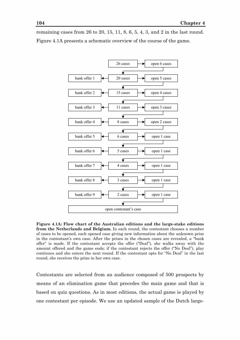
Chapter 4 104

remaining cases from 26 to 20, 15, 11, 8, 6, 5, 4, 3, and 2 in the last round.

Figure 4.1A presents a schematic overview of the course of the game.

Figure 4.1A: Flow chart of the Australian editions and the large-stake editions from the Netherlands and Belgium. In each round, the contestant chooses a number of cases to be opened, each opened case giving new information about the unknown prize in the contestant’s own case. After the prizes in the chosen cases are revealed, a “bank offer” is made. If the contestant accepts the offer (“Deal”), she walks away with the amount offered and the game ends; if the contestant rejects the offer (“No Deal”), play continues and she enters the next round. If the contestant opts for “No Deal” in the last round, she receives the prize in her own case.

Contestants are selected from an audience composed of 500 prospects by

means of an elimination game that precedes the main game and that is

based on quiz questions. As in most editions, the actual game is played by

one contestant per episode. We use an updated sample of the Dutch large-

15 cases

11 cases

8 cases

6 cases

5 cases

4 cases

3 cases

2 cases

bank offer 4

bank offer 5

bank offer 6

bank offer 7

bank offer 8

bank offer 9

bank offer 3

20 cases bank offer 1

26 cases

open contestant’s case

bank offer 2

open 5 cases

open 4 cases

open 3 cases

open 2 cases

open 1 case

open 1 case

open 1 case

open 1 case

open 1 case

open 6 cases

Risky Choice and the Relative Size of Stakes 105

stake episodes analyzed in PVBT, consisting of all the 56 episodes (292

choice observations) aired up to June 3, 2007. Because the €7,500 prize

was replaced with a €750,000 prize after episode 47, the average prize is

not exactly constant across all episodes, and equals €391,411 in episodes 1

– 47 and €419,696 in episodes 48 – 56. There were no further material

changes.

The Dutch small-stake edition uses only 20 prizes instead of 26. The prizes

are considerably smaller than in the large-stake edition, and range from

€1 to €250,000 with an average prize of €31,629. The game starts with 20

potential contestants, all randomly assigned a case with one of the 20

prizes hidden inside. A multiple choice question determines which

contestants qualify for a pool from which one contestant is then randomly

chosen to play the game. The 19 contestants that are not selected return

in the subsequent episode (together with one new contestant), to form the

group from which the next episode’s contestant is chosen. The small-stake

edition has a maximum of 5 rounds. In the first round, 6 cases are opened,

followed by 3 cases in each subsequent round. Figure 4.1B presents an

overview of the small-stake game. The first season of the small-stake

edition started on August 27, 2006 and episodes were then aired nearly

every weekday until June 8, 2007. Our sample consists of the full set of

204 episodes (904 choice observations) aired during this first season. All

the episodes were recorded by the authors. There were no changes to the

game format during the sample period. An occasional special feature in

the small-stake edition is the “swap option”. In the fifth game round of 24

episodes, when two cases or prizes are left, the contestant was offered the

opportunity to swap her case for the other remaining case. Whenever this

option was offered, it was always offered in addition to and not instead of a

regular bank offer. In most instances (16), the contestant preferred to stick

with her own case. Obviously, the opportunity to swap cases does not

change the contestant’s optimal strategy, because she has no information

about which of the two remaining prizes is her own case, and therefore we

do not pursue this option further.

Chapter 4 106

Figure 4.1B: Flow chart of the small-stake edition from the Netherlands.

The Belgian large-stake edition is named after the Dutch large-stake

edition, or “Miljoenenjacht”. The game uses 26 prizes with an average

value of €85,972, including a top prize of €1,000,000. The game is played

in exactly the same manner as the Dutch large-stake version (see also

Figure 4.1A). Contestant selection also occurs in the same way, although

the elimination game starts with only 150 prospects in the audience. The

Belgian large-stake version was aired 19 times, in two seasons of weekly

episodes. The first series of 11 shows was launched on October 16, 2004

and the second series of 8 shows started on October 15, 2005. Copies of the

19 shows (114 choice observations) were obtained from Endemol’s local

production company Endemol België.

A small-stake Belgian version called “Te Nemen of Te Laten” was launched

on August 21, 2006 and aired on most weekdays until April 12, 2007.

Unlike other editions, in this edition the contestant has to split her

winnings with an anonymous viewer. After adjustment, the top prize is

€100,000 and the average €11,492. Games are played in a maximum of 6

rounds, during which the number of cases, 22 at the start of the game,

decreases to 16, 13, 10, 7, 4, and finally 2; see Figure 4.1C. The contestant

14 cases

11 cases

8 cases

5 cases

2 cases

bank offer 3

bank offer 4

bank offer 5

bank offer 2

20 cases

open contestant’s case

bank offer 1

open 6 cases

open 3 cases

open 3 cases

open 3 cases

open 3 cases

open 1 case

Risky Choice and the Relative Size of Stakes 107

is randomly selected from a pool of 22 potential contestants, and, as in the

Dutch small-stake version, contestants that are not selected return in the

subsequent episode to form part of the group from which the next episode’s

contestant is selected. A typical feature of the Belgian small-stake game is

that, at some point during the game, most contestants are offered the

opportunity to exchange their case for any other remaining case. Contrary

to the swap option in the Dutch small-stake version, the offer to swap

cases replaces the regular bank offer for that particular round of the game.

It is the decision of the game-show producer as to if and when this offer is

made. As a result, contestants in the Belgian small-stake version may

experience some ambiguity beyond the normal risk of the game. A Belgian

colleague of the authors recorded all the 130 episodes. We deliberately

excluded one contestant from our sample (a Belgian celebrity playing on

behalf of a charitable institution on New Year’s Day; inclusion would not

have affected our results), leaving a sample size of 129 contestants (613

choice observations).

Figure 4.1C: Flow chart of the small-stake edition from Belgium.

22 cases

16 cases

13 cases

10 cases

7 cases

4 cases

2 cases

bank offer 1

bank offer 2

bank offer 3

bank offer 4

bank offer 5

bank offer 6

open contestant’s case

open 6 cases

open 3 cases

open 3 cases

open 3 cases

open 3 cases

open 2 cases

open 1 case

Chapter 4 108

In Australia, DOND made its debut on July 13, 2003. The first season

consisted of 14 weekly episodes, covering the games of 16 contestants (the

games of some contestants started in one episode and continued in the

next). The top prize of the 26 prizes in this large-stake version is

A$2,000,000 (€1,200,000 using a rate of €0.60 per A$), and the average

equals A$154,885 (€92,931). The structure of the game is exactly the same

as that of the large-stake versions in the Netherlands and Belgium (see

also Figure 4.1A), and the contestant is selected in a similar way (by

means of quiz questions) from a large group of prospects (200) in the

audience. Four additional Australian shows with large prizes were aired

as “special episodes” in August and September 2004. We have added two

of these shows to our sample: one with a couple playing the game and one

with an unlucky contestant from an earlier episode. A special episode with

hypothetical stakes (a former, lucky contestant playing on behalf of an

anonymous, ex-post selected viewer) and a show named “test of the

psychics” (where decisions were based primarily on clairvoyance) have

been intentionally omitted, although their inclusion would not affect our

results. Our Australian large-stake sample totals 18 contestants (100

choice observations); copies of the episodes were obtained from an

Australian game-show collector.

DOND returned to Australian TV on February 2, 2004, but as a shorter,

daily edition with considerably reduced prizes. The structure of the game

remained unchanged, but the top prize and the average prize were scaled

down to A$200,000 (€120,000) and A$19,112 (€11,467), respectively. The

contestant is selected from of a group of 26 by means of three multiple

choice quiz questions. Our sample covers the complete set of 140 episodes

(993 choice observations) aired up to August 13, 2004. After that date,

game options known as “Chance” and “Supercase” were introduced. These

options add ambiguity to the game that we prefer to avoid. We are grateful

to Endemol Southern Star and TV station Seven for providing us with the

recordings.

Risky Choice and the Relative Size of Stakes 109Table 4.1 - Summary statistics

The table shows descriptive statistics for our six samples from the Netherlands (Panel A and B), Belgium (C and D) and Australia (E and F). Age is measured in years. Gender is a dummy variable with a value of 1 assigned to females. Education is a dummy variable that takes a value of 1 for contestants with bachelor-degree level or higher (including students) or equivalent work experience. Stop Round is the number of the round in which the bank offer is accepted, or the maximum number of rounds + 1 for contestants who rejected all offers. Best Offer Rejected is the highest percentage bank offer the contestant chose to reject (“No Deal”). Offer Accepted is the percentage bank offer accepted by the contestant (“Deal”), or 100 percent for contestants who rejected all offers. Amount Won equals the accepted bank offer in Euros, or the prize in the contestant’s own case for those contestants who rejected all offers. Australian Dollars are converted into Euros by using a single fixed exchange rate of €0.60 per A$.

Mean Stdev Min Median Max A. Dutch large-stake edition (56 contestants) Age (years) 45.80 11.53 21.00 43.50 70.00 Gender (female = 1) 0.30 0.46 0.00 0.00 1.00 Education (high = 1) 0.52 0.50 0.00 1.00 1.00 Stop Round 5.23 1.73 3.00 5.00 10.00 Best Offer Rejected (%) 54.62 32.46 10.17 53.76 119.88 Offer Accepted (%) 74.68 30.92 20.77 79.23 165.50 Amount Won (€) 231,241.25 261,212.29 10.00 156,500.00 1,495,000.0B. Dutch small-stake edition (204 contestants) Age (years) 34.42 10.57 19.00 33.00 67.00 Gender (female = 1) 0.49 0.50 0.00 0.00 1.00 Education (high = 1) 0.38 0.49 0.00 0.00 1.00 Stop Round 4.74 0.95 3.00 4.00 6.00 Best Offer Rejected (%) 41.83 33.54 7.95 26.50 223.48 Offer Accepted (%) 64.82 34.60 9.51 53.69 188.94 Amount Won (€) 11,762.09 12,350.22 1.00 9,140.00 69,000.00 C. Belgian large-stake edition (19 contestants) Age (years) 41.89 10.11 30.00 42.00 65.00 Gender (female = 1) 0.21 0.42 0.00 0.00 1.00 Education (high = 1) 0.26 0.45 0.00 0.00 1.00 Stop Round 6.11 2.00 4.00 6.00 10.00 Best Offer Rejected (%) 55.96 26.56 20.70 49.83 114.29 Offer Accepted (%) 65.48 23.69 37.22 62.76 100.00 Amount Won (€) 50,263.16 48,886.88 500.00 30,000.00 200,000.00 D. Belgian small-stake edition (129 contestants) Age (years) 32.43 9.03 19.00 30.00 59.00 Gender (female = 1) 0.67 0.47 0.00 1.00 1.00 Education (high = 1) 0.33 0.47 0.00 0.00 1.00 Stop Round 5.71 1.11 4.00 6.00 7.00 Best Offer Rejected (%) 54.41 41.48 11.39 43.00 346.90 Offer Accepted (%) 74.08 28.50 14.56 79.79 140.00 Amount Won (€) 5,134.75 6,154.72 0.01 3,750.00 37,500.00

Chapter 4 110Table 4.1 (continued)

Mean Stdev Min Median Max E. Australian large-stake edition (18 contestants) Age (years) 32.33 6.32 20.00 32.50 43.00 Gender (female = 1) 0.25 0.43 0.00 0.00 1.00 Education (high = 1) 0.72 0.46 0.00 1.00 1.00 Stop Round 5.78 2.39 2.00 5.00 10.00 Best Offer Rejected (%) 63.53 47.55 8.99 53.70 178.09 Offer Accepted (%) 92.92 63.32 14.51 70.90 228.01 Amount Won (€) 56,922.00 83,917.34 3.00 27,075.00 309,000.00 F. Australian small-stake edition (140 contestants) Age (years) 36.04 11.89 18.00 35.00 75.00 Gender (female = 1) 0.50 0.50 0.00 0.50 1.00 Education (high = 1) 0.56 0.50 0.00 1.00 1.00 Stop Round 7.20 1.71 3.00 7.00 10.00 Best Offer Rejected (%) 77.38 30.15 15.69 75.59 184.62 Offer Accepted (%) 111.54 245.13 26.72 88.53 2.962.96 Amount Won (€) 9,899.96 12,766.19 0.30 6,783.00 120,000.00

For all episodes analyzed in this study, we collected data on the eliminated

and remaining prizes, the bank offers and the DOND decisions. We also

collected data on each contestant’s gender, age and education. Gender and

education are coded as dummy variables, with a value of 1 assigned to

females, and to contestants with either a bachelor degree level of

education or higher (including students) or equivalent work experience,

respectively. The contestant characteristics are in some instances obtained

from the producer, but mostly extracted from the introductory talk, from

other conversations between the host and the contestants, or from a short

movie about the life of the contestant at the beginning of some editions.

The contestant’s level of education is usually not explicitly mentioned, but

this characteristic can often be inferred from her stated profession.

Missing values for the contestant’s age are estimated on the basis of both

the contestant’s physical appearance and other helpful information such

as the age of children.

Table 4.1 presents summary statistics for the six samples. The average

age of the contestants varies from 32 (Australian large-stake edition) to 46

(Dutch large-stake edition), the proportion of women in the samples varies

from 21 (Belgian large-stake edition) to 67 percent (Belgian small-stake

Risky Choice and the Relative Size of Stakes 111

edition), and the average percentage of highly-educated contestants

ranges between 26 (Belgian large-stake edition) and 72 (Australian large-

stake edition). Despite some differences in the composition of the samples,

the variation within each sample is large, and the next section shows that

the contestant characteristics do not have a systematic and significant

effect across the different analyses.

Apart from one exception in the Australian large-stake edition,

contestants always reject the first two offers. Since the bank offer is only a

small fraction of the average remaining prize in the first rounds (as

illustrated in Table 4.2 discussed below), the choices in these rounds are

generally trivial. Statistics on the round in which contestants accept the

bank offer in each sample cannot be directly compared due to differences

in the maximum number of rounds in each edition. However, contestants

generally play for longer in editions with smaller stakes and in editions

with fewer cases to open per round. The same pattern emerges in

comparisons of the percentage bank offers that contestants choose to reject

and accept, suggesting a pattern of increased risk aversion for larger

stakes.4 In the next sections, we will show that this pattern across editions

is rather weak compared to the strong pattern of increased risk aversion

for larger stakes within each edition.

Performing the natural experiment with the same monetary prizes in the

lab would far exceed any experimental research budget as the combined

total prize money in the six samples equals nearly €85 million. The biggest

winner is a Dutch contestant named Helma: in the episode aired on

November 13, 2005, she accepted a bank offer of €1,495,000 in round 7,

while amounts of €1,000, €75,000, €2,500,000 and €5,000,000 were

remaining. Her case turned out to contain €1,000.

4 In Table 4.2, the average percentage bank offer accepted in the Australian small-stake edition is heavily influenced by one extremely appealing offer of 2,963 percent. Omitting this one observation reduces the average from 111.54 to 91.03 percent. In Table 4.3, omission reduces the reported average bank offer for round 9 from 198 to 103 percent.

Chapter 4 112Table 4.2 - Bank offers, stakes and decisions

The table summarizes the percentage bank offers, the stakes and contestants’ decisions for our six samples from the Netherlands (Panel A and B), Belgium (C and D) and Australia (E and F). The number of unopened cases when the bank offer is presented (Cases), the average bank offer as a percentage of the average remaining prize (%BO), the average remaining prize in Euros (Stakes), the number of contestants in the given round (No.), the number of those contestants that accept the bank offer (“D”) and the number of those contestants that reject the bank offer (“ND”) are reported for each round. Australian Dollars are converted into Euros by using a single fixed rate of €0.60 per A$. Observations with no bank offer (which occasionally occur when only insignificant amounts remain or due to a substituting swap offer) are excluded.

Round Cases %BO Stakes No. “D” “ND” A. Dutch large-stake edition

0 26 - 396,001 56 - - 1 20 6% 397,392 56 0 56 2 15 14% 386,686 56 0 56 3 11 33% 384,339 56 10 46 4 8 58% 360,429 46 13 33 5 6 75% 316,743 33 8 25 6 5 87% 238,631 25 13 12 7 4 96% 268,389 12 6 6 8 3 94% 139,341 6 4 2 9 2 106% 11,253 2 1 1

B. Dutch small-stake edition 0 20 - 31,629 204 - - 1 14 6% 30,888 204 0 204 2 11 12% 30,138 204 0 204 3 8 21% 30,473 204 11 193 4 5 41% 29,835 193 92 101 5 2 80% 18,203 99 40 59

C. Belgian large-stake edition 0 26 - 85,972 19 - - 1 20 6% 85,299 19 0 19 2 15 17% 79,160 19 0 19 3 11 34% 79,785 19 0 19 4 8 48% 87,566 19 5 14 5 6 60% 84,975 14 4 10 6 5 70% 73,546 10 3 7 7 4 78% 88,542 7 3 4 8 3 93% 5,809 4 1 3 9 2 101% 4,883 3 1 2

D. Belgian small-stake edition 0 22 - 11,492 129 - - 1 16 7% 11,441 129 0 129 2 13 16% 11,480 129 0 129 3 10 30% 11,482 127 0 127 4 7 39% 11,558 104 23 81 5 4 62% 10,205 71 34 37 6 2 87% 7,031 53 29 24

Risky Choice and the Relative Size of Stakes 113Table 4.2 (continued)

Round Cases %BO Stakes No. “D” “ND” E. Australian large-stake edition

0 26 - 92,934 18 - - 1 20 9% 84,804 18 0 18 2 15 15% 92,287 18 1 17 3 11 27% 107,131 17 2 15 4 8 65% 97,144 15 3 12 5 6 87% 109,683 12 4 8 6 5 95% 125,259 8 1 7 7 4 94% 112,308 7 3 4 8 3 120% 4,335 3 1 2 9 2 140% 2,254 2 1 1

F. Australian small-stake edition 0 26 - 11,467 140 - - 1 20 10% 11,132 140 0 140 2 15 22% 11,089 140 0 140 3 11 31% 11,678 140 1 139 4 8 49% 11,850 139 10 129 5 6 62% 11,557 129 14 115 6 5 78% 11,338 115 19 96 7 4 86% 11,447 96 32 64 8 3 102% 10,543 64 34 30 9 2 198% 9,649 30 15 15

Table 4.2 summarizes the offers made by the banker and the contestants’

decisions to accept or reject the offers in the various rounds. The offers are

related to the set of remaining prizes and typically start at a small fraction

of the average prize and approach 100 percent in the later rounds. As the

offers become more generous, more and more contestants are persuaded to

accept them (“Deal”) and exit the game. The bank offers in the last few

rounds of the Dutch and Belgian small-stake editions are relatively

conservative compared to those in the other editions. For example, in

round 6 of the Dutch large-stake edition and in round 4 of the Dutch

small-stake edition, five cases remain unopened. While in the large-stake

edition the banker on average offers 87 percent of the average remaining

prize, this percentage is only 41 in the small-stake edition. This difference

may reflect the fact that contestants in the small-stake edition generally

face more risk, because they have to open more cases. (For example, in

round 4, three out of five remaining cases have to be opened after a “No

Deal” decision, while this is only one out of five in round 6 of the large-

Chapter 4 114

stake edition.) Alternatively, if there are fewer rounds and smaller stakes,

there may be more incentive for the producer to discourage a “Deal” in

order to enhance the show’s entertainment value.

The next section uses probit regression analysis to analyze the DOND

choices in greater detail. We will perform regressions for each edition

separately, and for the combination of each pair of editions from the same

country. Comparing two editions from one country circumvents the

problems that may arise as a result of using editions from different

countries, like differences in wealth and culture (e.g. see Weber and Hsee,

2000, for the influence of culture on risk preferences). Although the small-

stake editions in both the Netherlands and Belgium have a somewhat

different structure than their large-stake counterparts, the effect of the

differences on the risk of continuing play are simple to model. The next

section shows that the choices in the various editions are not significantly

different after correcting for the percentage bank offers and the risk of

continuing play.

In addition to differences in the structure, there are also the possible

differences in the contestant pools. One concern is that richer and less

risk-averse people may be more willing to spend time attempting to get

onto a large-stake show than onto a small-stake one. Also, small-stake

editions generally feature contestants that are explicitly selected on an

individual basis by the producer, whereas chance plays a larger role in

selecting the people that play the elimination game in a large-stake show.

In the Dutch large-stake version for example, a national lottery sponsors

the show and the original 500 people in the audience are randomly invited

lottery players. Indeed, as shown above, the contestant characteristics

show non-trivial variation across the various editions. To account for the

contestant pool, we included these characteristics as control variables in

the regressions. The characteristics do not however show a systematic and

significant effect on the risk attitudes within the editions and it therefore

seems unlikely that they have a material effect across the editions.

Risky Choice and the Relative Size of Stakes 115

Moreover, our findings are confirmed in a series of experiments that

provide adequate controls for all these factors.

4.3 Probit regression analysis This section uses probit regression analysis to explain the DOND choices

within and across the various samples.5 The DOND choices of the different

contestants in different editions, different games and different rounds

cannot be directly compared without accounting for differences in the

game situations and contestant characteristics. Therefore, earlier DOND-

based studies like PVBT use structural choice models. The results of these

models are however sensitive to their precise specifications (for example,

the shape of the utility function and the dynamics of the reference point).

To avoid this problem, we estimate reduced-form models using probit

regression analysis rather than full-blown structural models, allowing for

a more compact presentation and more robust results.

The dependent variable is the contestant’s decision, with a value of 1 for

“Deal” and 0 for “No Deal”. We try to explain the decisions we observed

with the following set of contestant- and game-related variables:

- Age;

- Gender (0 = male, 1 = female);

- Education (0 = low, 1 = high);

- EV/105: absolute stakes, measured as the current average

remaining prize in Euros divided by 100,000;

- EV/EV0: relative stakes, measured as the current average

remaining prize divided by the initial average;

- BO/EV: percentage bank offer, or bank offer divided by the average

remaining prize;

5 Using logit instead of probit yields similar results.

Chapter 4 116

- Stdev/EV: standard deviation ratio, or standard deviation of the

distribution of the average remaining prize in the next round

divided by the average remaining prize.

The standard deviation ratio measures the risk of continuing play (“No

Deal”) for one additional round, and in this way accounts for the

differences between rounds and editions with respect to the number of

cases that have to be opened. Our video material suggests that the typical

contestant generally looks ahead to the bank offer in the next game round,

rather than to the prize in their own case; the game-show host, for

example, tends to stress what will happen to the bank offer in the next

round should particular cases be eliminated and the contestants

themselves often comment that they will play “just one more round”. The

use of other risk measures, such as the standard deviation of the

remaining prizes, tends to lower the empirical fit, but does not change our

conclusions regarding the relevance of relative stakes compared to

absolute stakes. Although the distributions of bank offers and prizes are

generally highly skewed, skewness does not add significant explanatory

power, because it is very strongly correlated with standard deviation in

this game.

To control for the attractiveness of the bank offer, we include the

percentage bank offer, which is defined as the bank offer divided by the

average remaining prize. The use of the inverse of the percentage bank

offer (which measures the expected return from rejecting the current and

subsequent bank offers) yields similar results and does not change any of

our conclusions.

Our focus is on the effect of absolute and relative stakes. The other

variables are included as control variables. Fortunately, the control

variables are only weakly correlated with the stakes variables so it is not

difficult to separate their effect. For example, the level of the stakes within

a given edition is determined by chance and therefore uncorrelated with

Risky Choice and the Relative Size of Stakes 117

the contestant characteristics. Since absolute and relative stakes are

perfectly correlated within each individual edition, only the absolute-

stakes variable is included as regressor in the one-sample analyses.6 Using

relative stakes in those analyses would yield the same results, the only

difference being that the absolute-stakes coefficient is multiplied by the

constant term EV0/105.

To allow for the possibility that the errors of individual contestants are

correlated, we perform a cluster correction on the standard errors (see, for

example, Wooldridge, 2003).

Table 4.3 shows the probit estimation results. The contestant

characteristics generally do not have significant explanatory power or at

least not consistently across all editions and countries, confirming the

results of PVBT (2008, Section II). In contrast, game characteristics have a

significant effect (with a few exceptions in the smaller samples) and show

a consistent pattern across all editions and countries. Our discussion

therefore focuses on the game characteristics.

Panel A shows the results for the Netherlands. As expected for non-

satiable and risk averse individuals, the “Deal” propensity increases with

the generosity of the bank offer and the dispersion of the outcomes.

Finally, the “Deal” propensity also increases with the stakes, consistent

with increasing relative risk aversion.

The results for the Dutch small-stake edition are very similar to those for

the large-stake edition, supporting our assumption that the two versions

of DOND are indeed comparable (after a proper correction for game

characteristics). However, for the small-stake edition, the coefficient for

the absolute-stakes term changes from 0.153 to 2.179, an increase of

roughly a factor of 14. Interestingly, this change is of the same order of

magnitude as the difference in the initial average prize of the two editions

(roughly a factor of 12.5). Replacing absolute stakes with relative stakes

6 In fact, for some of the editions analyzed in this study the correlation is marginally below unity due to small changes in the initial set of prizes.

Chapter 4 118

yields comparable coefficients for the two samples: 0.596 for the large-

stake sample and 0.689 for the small-stake sample (not reported in the

table). This is a first, strong indication that relative stakes in this game

matter more than absolute stakes.

The last three columns show the pooled results. If the stakes are included

in absolute terms, the empirical fit of the pooled sample (a log-likelihood of

-347.5) deteriorates significantly relative to the individual samples (LL = -

93.6 + -217.7 = -311.3), reflecting the very different absolute-stakes

coefficients in the two samples. However, if the stakes are measured in

relative terms, the fit of the pooled sample (LL = -333.0) is much more

comparable to the fit of the individual samples. Including both the

absolute and the relative-stakes variables hardly improves the

explanatory power (LL = -331.3) compared to using the relative-stakes

variable only.

To summarize, while the sensitivity of the “Deal” propensity to the

absolute level of stakes is much higher in the small-stake edition, the

sensitivity to the relative level of stakes is comparable. The contestants

respond in a similar way to changes in the relative stakes in each sample,

even though the absolute stakes differ by a factor of 12.5. This suggests

that the choice behavior is highly reference dependent. Decisions appear

not to be based on an evaluation of the absolute amounts that are at stake,

as we would expect an expected utility maximizer to do, but on the relative

size of the amounts. A given bank offer or prize appears to be considered

as “large” in the context of a game where it lies in the upper range of the

initial set of prizes, and the same amount seems to be evaluated as “small”

in a game where it belongs to the lower range of prizes.

Risky Choice and the Relative Size of Stakes 119Table 4.3 - Probit regression results within countries

The table displays the results from the probit regression analyses of the DOND decisions in our large- and small-stake samples from the Netherlands (Panel A), Belgium (B) and Australia (C). The dependent variable is the contestant’s decision, with a value of 1 for “Deal” and 0 for “No Deal”. Age is measured in years. Gender is a dummy variable with a value of 1 assigned to females. Education is a dummy variable that takes a value of 1 for contestants with bachelor-degree level or higher (including students) or equivalent work experience. EV is the current average remaining prize in Euros and EV0 is the initial average. BO is the bank offer. Stdev measures the standard deviation of the distribution of the average remaining prize in the next game round. Australian Dollars are converted into Euros by using a single fixed rate of €0.60 per A$. Observations with no bank offer (which occasionally occur when only insignificant amounts remain or due to a substituting swap offer) are excluded. The first column shows the large-stake results, the second column shows the small-stake results and the last three columns show the results for the large- and small-stake samples from one country combined. Apart from the maximum likelihood estimates for the regression coefficients, the table reports the log-likelihood (LL), the mean log-likelihood (MLL), McFadden’s R-squared, and the number of observations. The p-values (within parentheses) are corrected for correlation between the responses of a given contestant (contestant-level cluster correction).

Large stakes Small stakes Pooled Pooled Pooled A. The Netherlands Constant -5.229 (0.000) -4.191 (0.000) -3.600 (0.000) -4.311 (0.000) -4.251 (0.000)Age 0.021 (0.085) -0.001 (0.890) 0.008 (0.130) 0.014 (0.009) 0.012 (0.042)Gender 0.057 (0.780) 0.045 (0.740) -0.043 (0.710) -0.002 (0.990) -0.019 (0.870)Education 0.009 (0.970) -0.255 (0.097) -0.078 (0.490) -0.035 (0.760) -0.068 (0.560)EV/105 0.153 (0.000) 2.179 (0.000) 0.148 (0.000) 0.057 (0.110)EV/EV0 0.624 (0.000) 0.538 (0.000)BO/EV 2.677 (0.000) 1.148 (0.000) 1.390 (0.000) 1.868 (0.000) 1.802 (0.000)Stdev/EV 3.597 (0.066) 3.345 (0.000) 2.787 (0.000) 2.567 (0.000) 2.690 (0.000)LL -93.6 -217.7 -347.5 -333.0 -331.3 MLL -0.321 -0.241 -0.291 -0.278 -0.277 McFadden R2 0.337 0.448 0.353 0.380 0.383 No. obs. 292 904 1196 1196 1196 B. Belgium Constant -5.158 (0.001) -4.399 (0.000) -3.692 (0.000) -4.256 (0.000) -4.194 (0.000)Age 0.006 (0.650) -0.004 (0.730) -0.000 (0.990) 0.005 (0.490) 0.002 (0.810)Gender -0.204 (0.430) 0.033 (0.860) -0.033 (0.820) -0.139 (0.350) -0.080 (0.590)Education 0.596 (0.017) 0.340 (0.076) 0.312 (0.043) 0.308 (0.051) 0.324 (0.038)EV/105 0.848 (0.000) 5.510 (0.000) 0.799 (0.000) 0.387 (0.040)EV/EV0 0.633 (0.000) 0.482 (0.001)BO/EV 2.044 (0.018) 0.510 (0.220) 0.389 (0.250) 0.834 (0.064) 0.736 (0.097)Stdev/EV 4.813 (0.031) 4.260 (0.000) 3.963 (0.000) 3.693 (0.000) 3.855 (0.000)LL -34.5 -134.2 -181.5 -177.2 -175.5 MLL -0.303 -0.219 -0.250 -0.244 -0.241 McFadden R2 0.282 0.460 0.388 0.403 0.408 No. obs. 114 613 727 727 727

Chapter 4 120Table 4.3 (continued)

Large stakes Small stakes Pooled Pooled Pooled C. Australia Constant -4.052 (0.007) -4.119 (0.000) -3.638 (0.000) -4.023 (0.000) -4.032 (0.000)Age -0.012 (0.786) -0.001 (0.890) -0.001 (0.778) -0.000 (0.959) -0.000 (0.987)Gender -0.772 (0.321) 0.339 (0.007) 0.261 (0.030) 0.255 (0.033) 0.270 (0.024)Education -1.415 (0.001) -0.162 (0.160) -0.246 (0.027) -0.213 (0.049) -0.231 (0.038)EV/105 0.636 (0.000) 2.976 (0.002) 0.478 (0.000) 0.209 (0.175)EV/EV0 0.342 (0.001) 0.294 (0.010)BO/EV 1.767 (0.000) 1.845 (0.000) 1.504 (0.000) 1.649 (0.000) 1.665 (0.000)Stdev/EV 6.439 (0.007) 3.219 (0.000) 3.544 (0.000) 3.494 (0.000) 3.495 (0.000)LL -27.1 -244.8 -284.7 -278.5 -277.5 MLL -0.271 -0.246 -0.261 -0.255 -0.254 McFadden R2 0.384 0.349 0.322 0.337 0.340 No. obs. 100 993 1093 1093 1093

Panel B and C show the results for Belgium and Australia, respectively.

For both pairs of samples from these countries the same pattern arises.

The sensitivity for absolute stakes is much lower in the large-stake edition

than in the small-stake edition (0.848 vs. 5.510 for Belgium, and 0.636 vs.

2.976 for Australia), while the sensitivity for relative stakes is comparable

(0.728 vs. 0.633 for Belgium, and 0.591 vs. 0.341 for Australia; not shown

in Table 4.3).7 Note that the relative-stakes coefficients are not only

comparable within each country, but also across the three countries

included in the analysis so far. Compared to the relative magnitude of the

stakes, the absolute-stakes variable hardly provides any contribution to

the empirical fit of the pooled samples. These findings strengthen our

interpretation that decisions are primarily based on the relative values of

the amounts at stake.

Various robustness checks did not change our results. For example, we

added a quadratic stakes term to the regression to analyze if the

relationship between deal propensity and stakes is non-linear. The linear

and quadratic terms combined can give a second-order Taylor series

7 The absolute- and relative-stakes coefficients for the Australian small-stake sample are rather small compared to the coefficients for the Australian large-stake sample. This is partly attributable to the choices of contestant Dean Cartechini, a very lucky contestant in the June 17, 2004 episode, who played the game to the end only to discover that he had the top prize of A$200,000 in his case. If we exclude the choices of this particular contestant from the regression, the absolute stakes coefficient increases from 2.976 to 4.009 and the relative stakes coefficient increases from 0.341 to 0.460.

Risky Choice and the Relative Size of Stakes 121

approximation to an arbitrary (twice continuously differentiable) function.

In each sample, the quadratic term is significantly negative, suggesting

that the deal propensity becomes less sensitive to stakes at higher stakes

levels. Nonetheless, the main conclusion about the importance of the

relative level of the stakes remains the same. When the stakes are

measured in absolute amounts, the differences between the quadratic

terms are of the same order of magnitude as the differences in the squared

initial average prize. Consequently, the empirical fit in the pooled samples

deteriorates significantly relative to the individual samples if the stakes

are measured in absolute terms, and is comparable to the fit in the

individual samples if the stakes are measured in relative terms. Although

including a squared stakes term improves the empirical fit, the additional

term is highly correlated with the linear term and the linear term is more

important. For the sake of parsimony, we therefore do not include the

quadratic terms in the reported analyses.

4.4 Evidence from other countries and cross-

country analyses The analyses in the last two sections used data from different editions

from the Netherlands, Belgium and Australia. Comparing different

versions from only one country mitigates the potential confounding effects

of wealth and culture. However, DOND has been aired in many other

countries too, including several other developed, Western countries, and it

would be interesting to see if we find similar effects of absolute and

relative stakes. In this section, we will therefore repeat our probit analysis

for samples from the US, the UK, Germany and Switzerland, and we will

also perform large, pooled-sample analyses across the ten different

editions. Table 4.4 shows summary statistics for the four additional

editions.

Chapter 4 122Table 4.4 - Summary statistics for the US, UK, German and Swiss edition

The table shows descriptive statistics for our samples from the US, the UK, Germany and Switzerland. Definitions are similar to Table 4.1. US Dollars, UK Pounds and Swiss Francs are converted into Euros by using single fixed rates of €0.80, €1.50 and €0.65, respectively. Mean Stdev Min Median Max A. US edition (53 contestants) Age (years) 34.98 10.03 22.00 33.00 76.00 Gender (female = 1) 0.57 0.50 0.00 1.00 1.00 Education (high = 1) 0.49 0.50 0.00 0.00 1.00 Stop Round 7.70 1.29 5.00 8.00 10.00 Best Offer Rejected (%) 80.98 17.57 44.04 83.52 112.00 Offer Accepted (%) 91.43 15.31 49.16 97.83 112.50 Amount Won (€) 98,035.66 95,556.94 4.00 75,200.00 371,200.00 B. UK edition (326 contestants) Age (years) 42.42 14.93 19.00 38.00 83.00 Gender (female = 1) 0.50 0.50 0.00 0.50 1.00 Education (high = 1) 0.27 0.45 0.00 0.00 1.00 Stop Round 5.38 1.23 3.00 5.00 7.00 Best Offer Rejected (%) 55.10 20.60 8.00 53.43 120.63 Offer Accepted (%) 72.45 23.56 12.66 74.23 104.00 Amount Won (€) 24,287.14 25,496.60 0.02 19,425.00 180,000.00 C. German edition (81 contestants) Age (years) 35.96 9.86 18.00 34.00 62.00 Gender (female = 1) 0.42 0.50 0.00 0.00 1.00 Education (high = 1) 0.47 0.50 0.00 0.00 1.00 Stop Round 7.95 1.57 4.00 8.00 10.00 Best Offer Rejected (%) 85.49 31.51 35.24 81.82 190.40 Offer Accepted (%) 93.17 19.19 51.52 94.08 159.84 Amount Won (€) 20,528.91 23,503.69 0.01 15,000.00 150,000.00 D. Swiss edition (89 contestants) Age (years) 40.20 10.06 18.00 40.00 60.00 Gender (female = 1) 0.49 0.50 0.00 0.00 1.00 Education (high = 1) 0.30 0.46 0.00 0.00 1.00 Stop Round 8.20 1.78 4.00 8.00 10.00 Best Offer Rejected (%) 79.25 16.71 35.25 84.05 104.89 Offer Accepted (%) 87.36 14.54 48.75 90.94 108.70 Amount Won (€) 11,413.64 13,634.22 0.03 7,150.00 78,000.00

The US, German and Swiss editions are similar to the Dutch and Belgian

large-stake version and to the two Australian versions analyzed in the

previous sections: the shows start with 26 cases, last for a maximum of 9

rounds, and the number of cases opened in each round is 6, 5, 4, 3, 2, 1, 1,

1 and 1 respectively; see Figure 4.1A.8 The UK version is somewhat

different, and resembles the small-stake versions from Belgium and the

8 The first 20 contestants in our sample from Germany actually started with 20 cases. Effectively, their games can be analyzed as if the first round was skipped.

Risky Choice and the Relative Size of Stakes 123

Netherlands. Some US, UK and Swiss contestants are offered the

opportunity to swap their case at some point during the game. We ignore

this option as, in common with the Dutch small-stake edition, it is offered

only sporadically, does not replace a monetary bank offer (apart from a

few exceptions in the UK), and is often rejected.

For the US, we use the same sample as in PVBT, which covers the first 53

contestants (402 choice observations) after the premiere on December 19,

2005. The stakes in the US are relatively large: the regular format has a

maximum prize of $1,000,000 and an average prize of $131,478. In our

sample, the average prize is even larger ($142,435), because six games

were played with higher amounts to mark the beginning and end of a

particular series of episodes.

We updated the German sample of PVBT with data from the series aired

from November 2006 to May 2007. This adds an extra 34 contestants and

brings the total to 81 (628 choice observations). Most new episodes were

recorded by an acquaintance of the authors, and the remainder were

kindly provided by Endemol Deutschland. The initial stakes across the 81

games amount to €25,335 (€26,347 for the first 20 contestants, €25,003 for

the other 61).

DOND was introduced on Swiss TV on September 1, 2004. We obtained

the first two seasons of 44 and 45 weekly episodes (691 choice

observations) from Schweizer Fernsehen. The initial average prize in each

of the 89 episodes of “Deal or No Deal – Das Risiko” is Fr.26,898 (€17,583

using €0.65 per Fr.) and the largest prize is Fr.250,000 (€162,500).

The UK version started on October 31, 2005 and was normally aired six

times a week. The game commences with 22 prizes averaging £25,712

(€38,568 using €1.50 per £) and includes a top prize of £250,000

(€375,000). Over the maximum number of 6 rounds, 5, 3, 3, 3, 3 and 3

cases are opened, respectively. Thanks to the frequency with which the

program was aired and the readiness of Endemol UK to provide us with

Chapter 4 124

recordings, we have collected a large sample covering all 326 episodes

(1656 choice observations) up to December 11, 2006.

Table 4.5 shows the probit estimation results. Again, contestant

characteristics are generally insignificant, while the game characteristics

are highly important in every sample. The “Deal” propensity increases

with the relative bank offer, with the dispersion of the prizes and with the

level of the stakes.

Table 4.5 - Probit regression results for the US, UK, German and Swiss edition

The table displays the results from the probit regression analyses of the DOND decisions in our four samples from the US (first column), the UK (second column), Germany (third column) and Switzerland (fourth column). Definitions are similar to Table 4.3. US Dollars, UK Pounds and Swiss Francs are converted into Euros by using single fixed rates of €0.80, €1.50 and €0.65, respectively.

US UK Germany Switzerland Constant -5.239 (0.000) -4.470 (0.000) -4.867 (0.000) -4.403 (0.000)Age -0.006 (0.740) 0.004 (0.220) 0.009 (0.258) 0.002 (0.812)Gender -0.228 (0.370) 0.020 (0.850) 0.146 (0.451) -0.465 (0.008)Education -0.279 (0.210) -0.263 (0.025) 0.081 (0.679) 0.042 (0.821)EV/105 0.515 (0.000) 1.706 (0.000) 2.460 (0.000) 3.336 (0.000)EV/EV0 BO/EV 3.447 (0.000) 2.827 (0.000) 1.545 (0.000) 2.430 (0.000)Stdev/EV 3.377 (0.000) 2.166 (0.000) 3.248 (0.000) 2.079 (0.000)LL -77.9 -417.6 -128.2 -135.2 MLL -0.194 -0.252 -0.204 -0.196 McFadden R2 0.463 0.387 0.386 0.287 No. obs. 402 1656 628 691

To facilitate a comparison of the absolute- and relative-stakes coefficients

across the various editions, Table 4.6 summarizes the results for all

samples by listing the absolute-stakes and relative-stakes coefficients from

each one-sample regression, including the earlier regressions for the

Netherlands, Belgium and Australia. Clearly, the variation in the

absolute-stakes coefficients is much larger than the variation in the

relative-stakes coefficients, consistent with the notion of relative

valuation. For example, the absolute-stakes coefficient in the Dutch large-

stake edition is roughly 36 times smaller than that in the Belgian small-

stake edition; since the absolute stakes differ between the two editions by

Risky Choice and the Relative Size of Stakes 125

roughly the same factor (34.5), the two relative-stakes coefficients are

almost identical. The sensitivity to the absolute level of the amounts at

stake is clearly negatively related to the initial average prize (EV0),

whereas the relative-stakes coefficient is roughly equal (≈ 0.6) across all

editions. (The results for the Australian small-stake edition appear

somewhat different from the rest, but, as explained in Footnote 7, the low

values can be attributed in part to the choices of only one single

contestant.)

Table 4.6 - Overview of absolute- and relative-stakes effects

The table provides an overview of the probit regression coefficients for the absolute- and relative-stakes variables in multivariate probit regressions of the DOND decisions in the various editions of the game show. Age, Gender, Education, BO/EV and Stdev/EV are included as control variables. The results for the absolute-stakes variable EV/105 are taken from Table 4.3 and Table 4.5. The coefficients for the relative-stakes variable EV/EV0 are obtained by substituting the absolute-stakes variable for this variable. Also included for each edition are the mean initial average of the prizes in the game ( 0EV ; in Euros), the number of contestants (No. cont.) and the number of DOND decisions (No. obs.). Editions are arranged in order of initial average prize.

No. No. Stakes

Sample EV0 Cont. obs. Absolute Relative Australia, small 11,467 140 993 2.976 0.341 Belgium, small 11,492 129 613 5.510 0.633 Switzerland 17,483 89 691 3.336 0.583 Germany 25,335 81 628 2.460 0.614 The Netherlands, 31,629 204 904 2.179 0.689 UK 38,568 326 1,656 1.706 0.658 Belgium, large 85,792 19 114 0.848 0.728 Australia, large 92,934 18 100 0.636 0.591 US 113,948 53 402 0.515 0.635 The Netherlands, 396,001 56 292 0.153 0.596

We conclude with a probit regression analysis for the large sample of

editions combined. Note that analysis is based on a very large dataset of

nearly 6,400 choices made by more than 1,100 different contestants. The

results are presented in Table 4.7. If the stakes are included in absolute

terms (first column), the empirical fit of the pooled sample (a log-likelihood

of -1726.0) is clearly worse than the fit of the model that includes the

stakes in relative terms (second column; LL = -1629.9). This result reflects

the differences in absolute-stakes coefficients across the samples and the

Chapter 4 126

similarity of the relative-stakes coefficients that we observed earlier.

Including both stakes terms substantially improves the fit (last column;

LL = -1620.5) compared to the absolute-stakes model, whereas the

improvement is rather limited compared to the relative-stakes model,

strengthening our interpretation that decisions are primarily driven by

the relative values of the amounts that are at stake, and to a much lesser

extent by their absolute monetary values.

Table 4.7 - Probit regression results across countries

The table displays the results from the pooled probit regression analyses across the ten different editions of DOND used in this study. The first column shows the large-stake results, the second column shows the small-stake results and the last three columns show the results for the large- and small-stake samples from one country combined. Definitions are the same as those in Table 4.3.

All samples All samples All samples Constant -3.287 (0.000) -4.069 (0.000) -4.062 (0.000)Age 0.001 (0.640) 0.004 (0.063) 0.003 (0.143)Gender -0.025 (0.630) -0.011 (0.827) -0.010 (0.839)Education -0.098 (0.055) -0.072 (0.180) -0.088 (0.099)EV/105 0.208 (0.000) 0.100 (0.001)EV/EV0 0.548 (0.000) 0.499 (0.000)BO/EV 1.481 (0.000) 1.730 (0.000) 1.735 (0.000)Stdev/EV 2.491 (0.000) 2.648 (0.000) 2.687 (0.000)LL -1726.0 -1629.9 -1620.5 MLL -0.270 -0.255 -0.253 McFadden R2 0.309 0.348 0.351 No. obs. 6393 6393 6393

4.5 Summary and concluding remarks The TV game show DOND is a natural laboratory for studying risky

choice. This study examines a unique dataset of approximately 6,400

choices from ten different editions and six different countries. The editions

employ different sets of prizes, and we use these differences to separate

the effects of the absolute and relative amounts at stake on risky choice.

In the first part of the analysis, we restrict ourselves to three comparisons

of a large-stake edition with a small-stake edition from the same country.

This type of analysis avoids the possible systematic differences between

countries that may arise when comparing editions from different

Risky Choice and the Relative Size of Stakes 127

countries. In the second part of the analysis, we combine the data from the

ten different editions and six different countries. Both types of analysis

suggest that the choices in DOND are highly sensitive to the context in

which they occur, as defined by the initial set of prizes in the game.

Contestants respond in a similar way to the relative level of stakes, even

though the absolute level of the stakes differs significantly across the

various editions. Amounts therefore appear to be primarily evaluated

relative to a subjective frame of reference rather than in terms of their

absolute monetary value.

To those still not convinced, we find similar (but unreported) results in

DOND samples of Hungary, India, Mexico, and Thailand.9 Moreover, we

perform a series of controlled experiments among business and economics

students, in which we vary the initial stakes by a factor of 10 (see PVBT

and Chapter 3 for a detailed description). The estimated coefficients and

improved fit for relative stakes, as well as the wide variation in

coefficients and minor improve in fit for absolute stakes, are similar to

those reported for our large stakes editions of developed Western

countries, as can be seen in Table 4.8.

Table 4.8 - Probit regression results for the experimental sample

The table displays the results from the probit regression analyses of the DOND decisions in our experimental sample. The first column shows the large-stake results, the second column shows the small-stake results and the last three columns show the results for the large- and small-stake experimental samples combined. Definitions are similar to Table 4.3.

Large stakes Small stakes Pooled Pooled Pooled Constant -5.453 (0.000) -4.863 (0.000) -3.763 (0.000) -5.140 (0.000) -5.145 (0.000)Gender 0.104 (0.628) 0.218 (0.328) 0.310 (0.052) 0.163 (0.294) 0.161 (0.294)EV/105 258.36 (0.000) 2393.1 (0.002) 157.08 (0.000) 10.128 (0.810)EV/EV0 0.971 (0.000) 0.952 (0.000)BO/EV 2.975 (0.000) 3.108 (0.000) 2.325 (0.000) 3.053 (0.000) 3.055 (0.000)Stdev/EV 3.104 (0.000) 1.837 (0.011) 1.990 (0.000) 2.416 (0.000) 2.418 (0.000)LL -63.6 -64.3 -145.6 -128.7 -128.7 MLL -0.232 -0.237 -0.267 -0.236 -0.236 McFadden R2 0.414 0.372 0.309 0.390 0.390 No. obs. 274 271 545 545 545

9 These results are available upon request.

Chapter 4 128

Our results seem consistent with an appraisal of outcomes that is roughly

proportional to the average prize at the outset of the game. Unfortunately,

incorporating such a frame of reference in structural choice models

appears difficult, among other things, because both the absolute and

relative size of stakes are important. In fact, the prospect theory model

with the dynamic reference point specification developed in PVBT (and

Chapter 3) leaves much room for improvement when implemented across

the samples. However, future research has to explore this issue in more

detail.

Chapter 5

Irrational Diversification;

An Experimental Examination of

Portfolio Construction

Diversification is an important task in many problems of decision making

under risk or uncertainty. A decision maker can optimize her return and

risk exposure by carefully spreading out scarce resources over various

choice alternatives. Unfortunately, diversification is generally a complex

task as infinitely many possible combinations have to be considered.

Indeed, psychological work by Tversky and Kahneman (1981) and Simon

(1979) suggests that diversification may be too complex for decision

makers too perform, and decision makers adopt various kinds of

simplifying diversification heuristics in practice, as first shown by

Simonson (1990) and Read and Loewenstein (1995). Due to these

heuristics, the framing of the decision problem often critically affects the

final decision (see for example Langer and Fox (2004) for more details).

The choices of participants in defined contribution pension plans are

a case in point, as shown among others by Benartzi and Thaler (BT; 2001)

and Huberman and Jiang (HJ; 2006). When the number of funds offered

(n) is relatively small, plan participants seem to employ a naïve

diversification strategy of investing an equal fraction (1/n) in all funds

offered in the plan. Thus, the number of funds chosen increases as the

number of funds offered increases and the fraction invested in equity

increases as the fraction of equity funds offered increases. This behavior

seems suboptimal because the framing of the investment decision doesn’t

alter the investor’s optimal asset allocation. Further, when the number of

Chapter 5 130

funds offered becomes larger, participants seem to apply the 1/n rule to a

subset of the funds offered. For example, in the HJ study, the median

number of funds chosen is three, compared with a median number of funds

offered of 13.1 HJ refer to this phenomenon as the “conditional 1/n

diversification heuristic”.

One possible explanation for the conditional 1/n heuristic is that decision

makers assign too much weight to the marginal distribution of the

outcomes of the individual choice alternatives. Decision makers may

exclude the alternatives that are unattractive (that is, they yield small

gains and large losses) when held in isolation, without fully accounting for

their possible diversification benefits. Decision makers may then apply the

heuristic to the remaining alternatives, possibly because the remaining

alternatives are very similar. This explanation is reminiscent of the

“Elimination-By-Aspects” (EBA) theory (Tversky, 1972). This theory says

that people compare alternatives on their most salient or desirable

features, and eliminate alternatives that fall short on these aspects. Payne

(1976) and Payne, Bettman and Johnson (1993) find that decision makers

may use simple strategies such as the EBA to reduce the choice set before

applying a more complex (trade off) strategy to the remaining alternatives.

The explanation is also consistent with the findings of Kroll, Levy and

Rapoport (1988) and Kroll and Levy (1992), who show that decision

makers are largely insensitive to statistical associations between

investment alternatives.

Such behavior can have important practical consequences. For example,

Barberis and Huang (2001) show that a number of ‘anomalous’ asset

pricing patterns naturally emerge in an economy in which investors care

about fluctuations in individual stocks instead of fluctuations in their

portfolio. Similarly, for pension plans, the conditional 1/n heuristic may

lead participants to focus on a subset of funds in a similar (attractive)

1 Similar results are found by Friend and Blume (1975), Goetzmann and Kumar (2005) and Polkovnichenko (2005) for individual stock portfolio holdings. They show that the median number of stocks held in a portfolio is two to three.

Irrational Diversification 131

asset class. In this respect, financial advisors stressing the benefits of

diversification between asset classes and plans including mixed-funds

could help improve investment decision making.

To further examine the nature and cause of portfolio construction

decisions and diversification heuristics, we perform a series of experiments

among highly motivated and financially trained subjects. The experiment

involves unusually high incentive compatible payoffs for experimental

research (on average a subject earns roughly €50), to make sure subjects’

decisions have substantial consequences. The experiment allows us to

minimize the cognitive complexity of the portfolio problems by using

simple tasks with known probabilities and outcomes. In addition, the

experiment entails a control for many complicating real-life facets of

portfolio construction decisions and avoid the situation where the decision

maker adopts a heuristic because the choice alternatives are not

sufficiently different or to diversify away estimation or ambiguity risk.

Our experiments use a series of well-defined and simple base lotteries

with a small number of equally likely states. One of the lotteries is very

unattractive when held in isolation but very attractive for diversification

purposes due to a negative statistical association with the other lotteries.

This lottery is included to test the hypothesis that decision makers

overweight the marginal distribution.

The observed diversification strategy for pension plans cannot be classified

unambiguously as rational or irrational, because the preferences and

expectations of the different participants are unknown. Still, the high

concentration to stocks suggests that the 1/n rule is applied mostly to

stock funds. Since diversification effects generally are stronger between

asset classes than within asset classes, this suggests that the observed

allocations are not rational.

Our experiment circumvents the problems surrounding inference about

rationality because the probability distribution is known to the subjects.

To analyze if the observed choices are rational, we use the criterion of

Chapter 5 132

first-order stochastic dominance (FSD), which is generally accepted as a

minimal requirement for rational behavior, both in expected utility theory

and many non-expected utility theories. Using the FSD portfolio efficiency

test of Kuosmanen (2004), we can directly test if a given allocation is

rational, without knowing the precise preferences of the subjects.

By contrast, previous experiments analyzing diversification behavior

either (i) design the choice problems such that only one efficient

alternative exists (Rubinstein, 2002), (ii) test if framing affects the choices

without considering the efficiency of the choices (Langer and Fox, 2004), or

(iii) test the efficiency of subject’s portfolio choices using the mean-

variance or second-order stochastic dominance (SSD) criterion (Kroll, Levy

and Rapoport, 1988, Kroll and Levy, 1992, and Levy, Levy and Alisof,

2004).2

However, we stress that testing rationality is not our end goal. Given the

limited computational ability of the subjects, and the complexity of

diversification, it may not be reasonable to expect completely rational

choice to begin with, even for our simple lotteries. Rather, our objective is

to detect patterns in the deviations from rationality in individual

diversification decisions, to explain these patterns and to analyze the

effect of the framing of the diversification problem.

Our findings are as follows. A large majority of subjects focus on a subset

of the lotteries, where the subsets chosen are consistent with the idea that

the subjects focus on the marginal distribution of the individual choice

alternatives. Subjects exclude the alternatives that are unattractive when

held in isolation, without fully accounting for their possible diversification

benefits. Subsequently, many subjects tend to select an equal-weighted

combination of the remaining lotteries, and this conditional 1/n heuristic 2 Kroll, Levy and Rapoport (1988) and Kroll and Levy (1992) study experimentally the Second-order Stochastic Dominance (SSD) efficiency of portfolio choices when diversifying between three possible risky assets, with different degrees of correlation, and between three risky assets and one riskless asset. Levy, Levy and Alisof (2004) experimentally test the SSD efficiency of portfolio choices when diversifying between one of five to nine possible risky mutual funds and a riskless fund, thereby investigating the homemade leverage decision.

Irrational Diversification 133

is applied even if it is highly irrational in terms of FSD portfolio

inefficiency. Contradicting the unconditional 1/n rule, only a few subjects

select an even allocation across all lotteries. Moreover, emphasizing the

diversification benefits rather than the marginal distribution of the

individual choice alternatives improves the decisions considerably. In

other words, subjects don’t appreciate the effect of diversification unless

these effects are clearly pointed out to them. In addition, adding irrelevant

alternatives influences portfolio decisions, suggesting that problem

presentation has an important effect on individual portfolio decisions.

The remainder of this study is structured as follows. Section 5.1 discusses

the experimental design and the subjects in our first experiment. Section

5.2 discusses our results. Finally, Section 5.3 presents concluding remarks

and suggestions for further research.

5.1 The experimental design We use a laboratory experiment to test the portfolio construction decisions

of individuals. In an experiment we can control the choice alternatives and

ensure that the probabilities and outcomes are known to the decision

maker. In this way, we are able to control for many complicating real-life

facets of portfolio construction decisions and minimize the complexity of

the portfolio construction problems. Moreover, we avoid the situation

where the decision maker adopts a heuristic because the choice

alternatives are not sufficiently different or to diversify away estimation

or ambiguity risk.

5.1.1 The basics of our experimental design

Our experiment consists of five main tasks (Task 1-5), each of which

contains three to five or four base lotteries (B1-B6), as shown in Table 5.1.

Chapter 5 134Table 5.1 Lotteries and tasks

This table summarizes the main tasks and lotteries used in our first experiment. Each task involves three or four base lotteries (X1, X2, X3 and X4) with an uncertain payoff in three possible scenarios (S1, S2 and S3) of equal probability (1/3). The base lotteries (X1, X2, X3 and X4) are a selection from the lotteries (B1, B2, B3, B4, B5 and B6).

Gain/Loss (€) Lottery S1 S2 S3

B1 -50 +25 +125 B2 -25 0 +75 B3 -75 +50 +25 B4 +50 -75 +25 B5* 0 -25 +75 B6† -37.5 +12.5 +100

* 42

112

15 BBB +=

† 221

121

6 BBB +=

Lotteries

Task X1 X2 X3 X4 Task 1 B1 B2 B3 - Task 2 B1 B2 B4 - Task 3 B1 B2 B5 - Task 4 B1 B2 B4 B6 Task 5 B1 B2 B5 B6

In designing the experiment we used a few basic principles. First, to limit

the cognitive complexity of the choice problem, we focus on a small

number of base lotteries and a small number of scenarios. Specifically, the

first three tasks use three main base lotteries (X1, X2 and X3) with a

payoff in three possible scenarios (S1, S2 and S3). This is the minimal

degree of complexity needed to distinguish between the unconditional

version of the 1/n rule (which yields an even allocation across three base

lotteries) and the conditional version (which yields an even allocation

across two base lotteries). The remaining tasks add one irrelevant

alternative (X4) to the three main base lotteries, allowing us to investigate

the framing effects caused by the addition of irrelevant alternatives.

Second, the subjects may diversify between the three base lotteries.

Obviously, this substantially increases the complexity of the problem,

because there are infinitely many combinations. To limit this complexity,

we focus on the convex hull of the base lotteries, or the case where all

convex combinations of the base lotteries allowed:

(5.1) ⎭⎬⎫

⎩⎨⎧

=≥== ∑=

3,2,10;1:),,(W3

1321 jwwwww j

jj

Irrational Diversification 135

with 1w , 2w and 3w for the weights assigned to X1, X2 and X3 respectively.

In this setup, negative positions are not allowed (no short sales), the

weights must sum to unit y (no riskless option) and no further restrictions

are placed on the weights. Presumably, short sales, a riskless option and

weight restrictions would substantially increase the complexity and

cognitive burden of the choice problem.

Third, to further limit the computational complexity of the diversifying

allocations and to limit possible effects of probability distortion we use

equal and moderate probabilities of 1/3 for every scenario.3 Although there

may be some probability distortion, this is not likely to influence are

inferences since the FSD rule used in our study is invariant to subjective

transformation of the cumulative probabilities (as in the Cumulative

Prospect Theory (CPT) of Tversky and Kahneman, 1992).

Fourth, to ensure that the experiments are realistic for investment

choices, all base lotteries are “mixed gambles” that involve both gains and

losses. Further, no combination of the base lotteries yields only gains. In

this way we hope to avoid situations in which subjects take more risk, by

investing only in the alternative with the highest mean because they have

no possibility to lose money.

Finally, to gauge the efficiency of subject’s choices we focus on the criterion

of FSD efficiency. A typical problem in gauging the outcomes of choice

experiments (as well as real-life choices) is that the preferences of the

subjects are not (fully) known or are constructed at the moment of the

decision (Payne, Bettman and Johnson, 1992, Slovic, 1995). This makes it

difficult to establish if observed diversification behavior is efficient and to

what degree. The criterion of FSD circumvents this problem, because it

does not require a precise specification of the preferences of the decision 3 Still, according to some decision theories like Cumulative Prospect Theory (Tversky and Kahneman, 1992) these equally likely probabilities may suffer from probability distortion. For example, the Cumulative Prospect Theory function and parameters of Tversky and Kahneman (1992) predict that the lowest outcome of each lottery is transformed to 0.35, the middle outcome to 0.18 and the highest outcome to 0.34. By contrast, Levy and Levy (2002) question the probability distortion of equal probabilities on each scenario, as predicted by Prospect Theory (Kahneman and Tversky, 1979).

Chapter 5 136

maker and applies for a broad class of preferences. According to the

traditional definition, a choice alternative with cumulative distribution

function )(xF FSD dominates another alternative with cumulative

distribution function )(xG if and only if )()( xGxF ≤ for all x with a strong

inequality for at least some x. Since FSD only requires that people prefer

more over less, it is a minimal requirement for rational behavior, both in

expected utility theory and many non-expected utility theories (for

example CPT). Descriptively, FSD also seems a good criterion, because

subjects seldom select an alternative that is FSD dominated if the

dominance is easily detected (Tversky and Kahneman, 1986).

A subject may use the 1/n rule or conditional 1/n rule simply because the

choice alternatives are not sufficiently different given her preferences. For

example, a risk-neutral subject will be indifferent between alternatives

that yield the same average outcome, irrespective of possible differences in

the distribution of the outcomes. To ensure that the allocations have a

substantial effect on the probability distribution of the outcomes, and

hence the FSD criterion will have discriminating power, the base lotteries

have to be constructed in such a way that they exhibit significant

differences in mean, dispersion and ranking of the outcomes in order.

5.1.2 The tasks

In Task 1, B3 has an unfavorable marginal distribution; it is FSD-

dominated by B1 since it involves a lower minimum (-75 vs. -50), the same

middle value (+25) and a lower maximum (+50 vs. +125). Also, B3 has

limited value for diversification purposes because it has a positive

statistical association with lotteries B1 and B2.

In Task 2, B3 is replaced with B4, which plays an important role in the

experiment. B4 is in fact a permutation of B3 and these two lotteries have

the same marginal distribution. When held in isolation, B4 is FSD-

dominated by B1 since it involves a lower minimum (-75 vs. -50), the same

Irrational Diversification 137

middle value (+25) and a lower maximum (+50 vs. +125). Still, B4 may be

interesting, because in contrast to B3, it has a negative statistical

association with lotteries B1 and B2, yielding possible diversification

benefits. In addition, B2 is FSD dominated by the simple combination of

investing 75% in B1 and 25% in B4. Furthermore, every combination that

contains a positive allocation to B2 can be shown to be FSD dominated by

some combination of B1 and/or B4. Subjects focusing only on the

alternatives with attractive marginal distributions are likely to oversee

the diversification benefits of B4 and hence are likely to make inefficient

choices.

In Task 3, B4 is replaced with B5, which equals the equal-weighted

average of B1 and B4, that is, =5B 421

121 BB + . Besides reducing the choice

set by excluding allocations to B4 greater than the allocations to B1, this

framing effect implies that the unfavorable marginal distribution of B4 is

no longer shown, while emphasizing the diversification benefits from

combining B1 and B4. In fact, 5B has the same marginal distribution as B2,

but offers greater diversification possibilities due to the negative

statistical association with B1.

In Task 4 and Task 5 we reframe the portfolio construction problem by

adding one simple, but irrelevant alternative to Task 2 or Task 3. In Task

4 (Task 5) we add B6 to Task 2 (Task 3), which is an equal weighted

combination of B1 and B2 (that is, =6B 221

121 BB + ). These additions do not

alter the choice set and formal choice problem, and should have no

influence on choices.4

5.1.3 Testing for FSD-efficiency: the Kuosmanen test

We will use the recently developed Kuosmanen (2004) mathematical

programming test for determining if a given combination of choice

4 In addition, we presented four related tasks (Task 6 to Task 9) to the subjects. The precise details about these tasks are available upon request.

Chapter 5 138

alternatives is FSD efficient, or non-dominated relative to all possible

combinations of the choice alternatives.

When applied to our experiment, the Kuosmanen (2004) test statistic for a

given allocation ),,( 321 www is computed by solving the following mixed

integer linear programming problem:

(5.2) ∑∑= =

−===

3

1

3

131

,321 )(max),,(

31,

31 j i

ijjijjpz

xwxzwwwjssjjj

θ

3,2,1 s.t.3

1

3

1

3

1=≥∑ ∑∑

= = =

ixwpxzj j s

sjjsjijj

3,2,113

1

==∑=

jps

sj

3,2,113

1==∑

=

spj

sj

1,0∈sjp

13

1=∑

=jjz

3,2,10 =≥ jz j

This problem seeks an allocation ),,( 321 zzz that always yields a higher

outcome than the outcomes of the chosen allocation ),,( 321 www or some

permutation of those outcomes. The outcomes are denoted by 31, =jiijx and

the permutation of the outcomes is represented by the binary

variables 31, =jssjp .

The test statistic ),,( 321 wwwθ has the compelling interpretation of the

maximum possible increase in the mean outcome that can be achieved

with a combination that FSD dominates the evaluated combination. Thus,

Irrational Diversification 139

if the test statistic takes a value of zero, the evaluated combination is FSD

efficient; if it takes a strictly positive value, the combination is FSD

inefficient.5

To illustrate the working of the Kuosmanen test in the context of our

experiment, consider a subject who excludes B4 from her choice set and

divides her money evenly between B1 and B2, that is, )0,,( 21

21 , in Task 2. As

shown in Table 5.2, a combination with 87 allocated to B1 and 8

1 to B4 or

),0,( 81

87 dominates this combination. In Scenario S1 and S2 the outcomes

remain -37.5 and +12.5 respectively. However, in S3 the outcome increases

from +100 to +112.5, leading to a possible increase of the mean

of =)0,,( 21

21θ 6

14 . Hence, a subject who applies the conditional 1/n rule over

lotteries B1 and B2 of Task 2 makes an FSD inefficient choice as she

forgoes at least 614 in terms of mean outcome.

Table 5.2 Example illustration of the Kuosmanen test

A: The FSD inefficient combination )0,,( 2

121

Gain/Loss (€) S1 S2 S3 %

B1 -50 +25 +125 50 B2 -25 0 +75 50 B4 +50 -75 +25 0

Total -37.5 +12.5 +100 100

B: The FSD dominating combination ),0,( 81

87

Gain/Loss (€) S1 S2 S3 %

B1 -50 +25 +125 87.5 B2 -25 0 +75 0 B4 +50 -75 +25 12.5

Total -37.5 +12.5 +112.5 100 5 One complication which is relevant for the analyst is that the efficient set is often not convex; combining two FSD efficient combinations does not always yield an FSD efficient combination. The non-convexity of the efficient set stems from the fact that the preferences are not known to the analyst and that very diverse preferences are admitted under the FSD rule. This complicates the testing of FSD efficiency for the analyst, but for the individual subject this problem is less relevant, because only her personal preferences are relevant for her decision and these preferences are known to her. We do not claim that the subject faces a simple problem but rather that she presumably doesn’t apply the FSD rule because she restricts her attention to her own preference rather than the entire set of preferences than admitted by the FSD rule.

Chapter 5 140

The FSD efficient sets

Figure 5.1A shows the values of the Kuosmanen test statistic (“the

maximum possible increase in the mean given risk”) for all feasible

combinations of 1w and 2w in Task 1. The weight 3w is not shown, because

it can be found as the residual 213 1 www −−= .

Despite the generality of the FSD criterion, the efficient set (all

combinations with a zero value for the test statistic) is only a small subset

of the entire choice set. For this task, the efficient set is given by:

(5.3) [ ]( ) [ ]( ) 0;1;1,01;0;1,:),,(W 312113251

1321*1 =−=∈∪−==∈= wwwwwwwwwww

In other words, either investing 80% percent or less in B3 ( 54

3 ≤w ) and the

remainder in B1 or investing nothing in B3 is efficient. Full investment in

B1 is efficient as it maximizes the expected pay-off. Since the three

alternatives have a strong statistical association, there are few

possibilities for diversification. Still, subjects may want to combine B1 with

B2 or B3 to reduce risk. However, allocations to B3 substantially reduce the

expected payoff of a portfolio, increase its downside risk and reduce its

upward potential, making these portfolios generally unattractive. Hence,

in Task 1, B3 has an unfavorable marginal distribution, both when seen in

isolation and for diversification purposes. The largest value for the test

statistic is achieved with full allocation to B3; 3133)1,0,0( =θ . The test

statistic generally increases as the allocation to B3 increases. Moreover,

using the unconditional 1/n heuristic of investing an even allocation in

each alternative ),,( 31

31

31 is highly inefficient with a value for the

Kuosmanen test statistic of 16.50.

Irrational Diversification 141Panel A: Task 1

0.0

0.5

1.00.0

0.5

1.0

0

5

10

15

20

25

30

35

Kuo

sman

en F

SD-te

st v

alue

w 2 w 1

Panel B: Task 2 & 4

0.0

0.5

1.00.0

0.5

1.0

0

5

10

15

20

25

30

35

Kuo

sman

en F

SD-te

st v

alue

y 2 y 1

Panel C: Task 3 & 5

0.0

0.5

1.00.0

0.5

1.0

0

5

10

15

20

25

30

35

Kuo

sman

en F

SD-te

st v

alue

y 2 y 1

Figure 5.1: FSD test statistic for Task 1 to Task 5 The figure shows the Kuosmanen test statistic values ),,( 321 wwwθ for all possible allocations of Task 1 to Task 5. The test statistic measures the maximum possible increase in the mean outcome that can be achieved with a combination that FSD dominates the evaluated combination. Thus, if the test statistic takes a value of zero, the evaluated combination is FSD efficient; if it takes a strictly positive value, the combination is FSD inefficient. Panel A shows the Kuosmanen test values for Task 1, Panel B shows the test values for Task 2 and Task 4, and Panel C shows the test values for Tasks 3 and 5. For the sake of comparability with Task 2, the weights of Task 3 to Task 5 are transformed to their implied allocations for Task 2. The implied allocation to B1 is denoted by 1y , the implied allocation to B2 by 2y and the implied allocation to B4 by 3y . The figure shows all feasible combinations of 1w (or 1y ) and

2w (or 2y ), using 10% intervals. The weight 3w (or 3y ) is not shown, because it can be found as the residual 213 1 www −−= (or 213 1 yyy −−= ).

Chapter 5 142

In Task 2, B3 is replaced with B4, which has a more favorable ranking

than B3. This replacement has an important effect on the efficient set,

since it introduces diversification benefits for B4. Figure 5.1B shows the

Kuosmanen test statistic values. For sake of comparability with later

tasks, we will denote the allocation in Task 2 by 1y , 2y and 3y .

Specifically, the efficient set in Figure 5.1B is given by

(5.4) 213285

41

81

1321*

4 & 2 1,0],1,[),[:),,(W yyyyyyyy −−==∪∈=

Thus, allocating a non-zero percentage to B2 can be shown to be FSD

inefficient. The largest value for the test statistic is achieved with full

allocation to B4; 3133)1,0,0( =θ . Nevertheless, allocating a small fraction

( 83

3 ≤y ) or a large fraction ( 87

343 ≤< y ) in B4 and the remainder in B1 does

yield an efficient combination. The risk neutral or seeking ‘homo-

economicus’ would select B1 alone, while the moderately risk averse ‘homo-

economicus’ would choose to mix B1 and B4 rather than B1 and B2 due to

the negative statistical association between B1 and B4. By contrast, the

non-‘homo-economicus’ subjects, who focus on the marginal distribution

without taking the diversification benefits into account, would exclude B4

from their choice set; B4 is (most) unattractive when held in isolation,

since it has the largest loss, smallest gain, and smallest expected value.

However, the simple combination of investing 75% in B1 and 25% in B4 is

always as least as good in every state as investing in B2, since it yields the

same outcomes in S1 and S2 and a better outcome in S3 (+100 vs. +75).

Hence, subjects incorporating statistical association in the formation of

their portfolios would exclude B2. Moreover, subjects following the

conditional diversification heuristic between B1 and B2 would make

inefficient choices; their maximum possible increase in expected payoff

without changing their (downside) risk is €4.17 (on an expected payoff of

€25). Similarly, subjects following the unconditional 1/n rule would have a

Kuosmanen test statistic of 5.56 in Task 2.

Irrational Diversification 143

Figure 5.1C shows the results for Task 3. In this task B4 is replaced with

B5, which equals the equal-weighted average of B1 and B4, that is,

=5B 421

121 BB + . Besides reducing the choice set by excluding allocations to

B4 greater than the allocations to B1, this framing effect implies that the

unfavorable marginal distribution of B4 is no longer shown, while the

diversification benefits from combining B1 and B4 over B2 are made

explicit. For the sake of comparability with Task 2 (Figure 5.1B) we will

transform the allocations chosen in Task 3 to their implied Task 2

weights; 1y includes both the direct allocation to B1 and half of the

allocation to B5. Thus, if 21 is allocated to B1 and 2

1 to B5, we have 43

1 =y .

Compared with Figure 5.1B, the most inefficient alternatives, which

involve a relatively high allocation to 4B , are now eliminated. The test

statistic now reaches its maximum at )0,1,0( and ),0,( 21

21 . Indeed, B2 and B5

have the same marginal distribution and hence full allocation to one of

these two lotteries yields the same value for the test

statistic; 31

21

21 8),0,()0,1,0( == θθ . However, B5 is more attractive for

diversification purposes. Related to this, all combinations with a non-zero

allocation to B2 are inefficient, while high allocations to B5 ( 83

3 >y ) are

also inefficient. Specifically, the efficient set for Task 3 is given by

(5.5) 213285

1321*

5 & 3 1;0];1,[:),,(W yyyyyyyy −−==∈=

As before, the unconditionally naïve diversification heuristic of investing

an even allocation in each alternative ),,( 31

31

31 is inefficient for every subject

in Task 3, with a Kuosmanen test statistic of 2.78.

In Task 4 (Task 5), we add the equal weighted combination of B1 and B2

(that is, =6B 221

121 BB + ) to Task 2 (Task 3). These additions keep the

efficient choice set exactly the same, implying that equation (5.4)

(equation (5.5)) give the efficient sets for Task 2 (Task 3), in terms of

Chapter 5 144

implied Task 2 allocations. For Task 4, the Kuosmanen test values are

shown in Figure 5.1B, while the Kuosmanen test values for Task 5 are

shown in Figure 5.1C. Overall, the same remarks applying to Task 2 (Task

3) also hold for Task 4 (Task 5), most important the fact that allocations to

B2 are inefficient. In addition, B6 consist for 50% of B2, implying that

positive allocations to this alternative will similarly result in inefficient

allocations.

5.1.4 Logical inference

In summary, while the probability distribution of the lotteries is

controllable by the analyst and known to the respondents, a key problem

of choice experiments is that the preferences of the respondents are not

fully known to the analyst. To avoid this problem, our logical inference is

based on two pillars: (5.1) the logical relationship between the choice sets

and the efficient sets in the choice tasks and (5.2) the FSD criterion

applying for all rational decision makers.

First, the choice sets and the efficient sets in the nine tasks are strongly

related. The difference between the first and the second task is only the

different ordering of the third lottery (B3 is replaced by B4). Since B4 in

contrast to B3 has a negative statistical association with B1 and B2, this

change leads to a substantial improvement in the diversification

possibilities for all rational respondents. Therefore, while in Task 1 the

focus could be mainly on the marginal distributions of the lotteries, the

focus in Task 2 should also be on the possible diversification benefits

between the lotteries. We thus expect improved choices and the only

reasonable explanation for failure to improve the choices seems that the

respondents do not fully account for the diversification benefits in the

second task and instead pay too much attention to the marginal

distributions of the lotteries.

Irrational Diversification 145

Similarly, the difference between the second and the third task is only the

replacement of the third lottery with the equal-weighted average of the

first and third lottery (B4 is replaced by B5). This leads to more directly

observable diversification benefits, but rational decision makers should

already have taken the diversification benefits into account in Task 2.

Hence, we expect similar choices and the only reasonable explanation for

improvements seems that the respondent is helped by the framing of the

choice problem – stressing the diversification benefits rather than the

marginal distributions.

In task 4 (Task 5) we add a simple combination of two presented

alternatives to Task 2 (Task 3), which has no influence on the formal

choice problem. Hence, we expect similar choices in Task 2 and Task 4

(Task 3 and Task 5) and the only reasonable explanation for differences

seems that the respondent is sensitive to the framing of the choice

problem – presenting additional but irrelevant alternatives.

Second, the general FSD criterion allows for classifying choices as efficient

or inefficient, without having to specify the exact preferences of the

respondents or adopting a specific theory of choice under risk. Of course,

the risk of this “nonparametric” approach is a lack of statistical power

(failure to identify inefficient choice). However, as we will see below, many

of the respondents in this experiment display a type of inefficient behavior

that can be detected even with the FSD rule.

As discussed in the introduction, testing rationality is not our end goal. In

fact, given the limited computational ability of the subjects, and the

complexity of choice problem, it may not be reasonable to expect

completely rational choice to begin with, even for our simple lotteries.

Rather, our objective is to detect and explain patterns in the deviations

from FSD-inefficient behavior and to analyze if these patterns are affected

by framing effects. For this purpose, the FSD efficiency test offers a useful

measure of rationality.

Chapter 5 146

5.1.5 The subjects

In total 107 third and fourth year undergraduate students of general

economics or financial economics participated. These students were

recruited during advanced courses on portfolio theory or financial

economics. At that stage of their studies, the students had completed at

least two basic courses in statistics, microeconomics and finance and thus

were familiar with formal decision making, probabilistic calculus and

portfolio theory. In addition, a formal requirement to participate in these

courses is that subjects have successfully completed a course on

Markowitz portfolio theory. Hence, we can expect that these students are

financially well trained and well aware of formal decision making,

probabilistic calculus and portfolio theory.

Appendix 5.A shows the format in which the tasks were presented to the

subjects (translated from Dutch to English). Answering the diversification

questionnaire took the subjects on average roughly one hour. Since the

choices were filled out on a paper form that is handed in after all tasks are

completed, the choices of previous tasks remained available to the subjects

during the course of the experiment. In addition, all subjects brought or

received a pocket calculator to help them in performing the necessary

calculations.

We use high incentive-compatible payoffs. Specifically, the subjects were

told that one of the nine tasks is selected at random and played for real

money at the end of the experiment. Each task is equally likely to be

selected. This incentive scheme has proven to be an effective tool in static

decisions problems like ours, since it avoids income effects while incentives

in each task are not diluted by the probability of payout (see Starmer and

Sugden, 1991, and Cubitt, Starmer and Sugden, 1998). Because there is a

possibility that subjects would loose money we ask each subject to bring

€25 to the experiment. Also, to cover possible losses each subject received

a show-up fee of €10 and received €15 for participating in another 30

minute questionnaire which took place after the current experiment. After

Irrational Diversification 147

each subject had completed her tasks we handled the payments by calling

the subjects forward, asking them to put their home brought €25 on table

and throwing dices to determine their earnings. Hence, subjects could only

lose out-of-pocket money if they were willing to take the risk of loosing

more than €25 in an individual task.6 The average subject took home

roughly €50, which in our view is a large amount for participating in a

one-and-a-half hour lasting experiment.

In a preliminary experiment without choice-related monetary incentives,

we found many errors of computation, suggesting that the subjects paid

less attention without monetary rewards. In this experiment, with

monetary rewards, no-one opted not to participate after reading the

instructions, made serious miscalculations or did not fill in the amounts

allocated to each lottery leaving us with a final sample of 107 subjects.

Moreover, the experiment reported here actually replaces an earlier,

similar experiment with a between-subject random-task-incentive-system

(see Baltussen, Post, Van den Assem and Wakker, 2008) in which some of

the subjects were randomly selected to play for real money. This incentive

scheme was abandoned, because the perceived incentives may be smaller

than originally intended. Encouragingly, the earlier experiment leads to

the same results and conclusions as reported here.

6 A possible objection to this incentive scheme is that it may stimulate investing 100% in B2 in each task. This to avoid the possibility that subjects had to pay out-of-pocket money, because the outcomes of the tasks are never worse than -€25, and thus at least cancels against the €25 they obtained by participating in the experiment and questionnaire. However this does not affect our results, because the FSD rule is invariant to endowments and because we study changes in choice behaviour across the tasks rather than the choices in a given task. Moreover, in Task 2 (Task 3) B2 is FSD-dominated by the relatively simple combination of investing 75% in B1 and 25% in B4 (50% in B1 and 50% in B5). These strategies perform never worse than B2 and yield a €8.33 higher expected payoff in both tasks. Hence, they are clearly superior to investing 100% in B2 for subjects who want to avoid out-of-pocket losses. Besides this, fulfilling the experiment and questionnaire took roughly 1 hour and 30 minutes. In our view, subjects do not see a zero outcome as a non-loss for devoting that much time to an experiment. In addition, the results in the next section show that not many subject opted for 100% investing in B2 (or B5) and exposed themselves to possible out-of-pocket losses (28.0% for Task 1 and on average 5.6% (3.7%) for Task 2 to 3).

Chapter 5 148Table 5.3 Summary of allocations

This table shows the main results of our experiment (107 subjects). For every task, the table shows the average allocations to each alternative, the average implied allocations to B1, B2 and B4, the proportion of subjects who excluded each alternative, the proportion of subjects who invested in one alternative, the numbers of funds chosen by the subjects, the percentage of equal splits between those funds chosen, the proportion of subjects who relied on a specific diversification heuristic, and the proportion of subjects who choose a FSD-inefficient allocation, as well as the average Kuosmanen test statistic in € and % over all allocations (Mean Inefficiency). For Task 1 to Task 5, w1 denotes the allocation to B1 and w2 denotes the allocation to B2.For Task 1, w3 denotes the allocation to B3, for Task 2 and Task 4, w3 denotes the allocation to B4, and for Task 3 and Task 5, w3 denotes the allocation to B5. For Task 4 and Task 5, w4 denotes the allocation to B6. For the sake of comparability with Task 2, the weights of Task 3 to Task 5 are also transformed to their implied allocations to B1, B2 and B4. The implied allocation to B1 is denoted by 1y , the implied allocation to B2 by 2y and the implied allocation to B4 by 3y .

Task 1 Task 2 Task 3 Task 4 Task 5 Average allocations w1 42.9% 51.8% 47.4% 40.0% 34.4% w2 54.2% 31.1% 16.9% 18.9% 17.7% w3 2.9% 17.1% 35.7% 17.1% 32.0% w4 - - - 24.1% 16.0% Average implied allocations to B1, B2 and B4 Y1 - 51.8% 65.3% 52.0% 58.3% Y2 - 31.1% 16.9% 30.9% 25.7% Y3 - 17.1% 17.9% 17.1% 16.0% Excluded alternatives w1=0 28.0% 9.3% 15.9% 18.7% 29.0% w2=0 18.7% 33.6% 54.2% 45.8% 52.3% w3=0 84.1% 43.0% 18.7% 39.3% 23.4% w4=0 - - - 40.2% 52.3% Invested in one alternative w1=1 17.8% 15.0% 15.0% 12.1% 13.1% w2=1 28.0% 9.3% 1.9% 5.6% 1.9% w3=1 0.0% 0.0% 3.7% 0.0% 1.9% w4=1 - - - 1.9% 2.8% Number of funds chosen 1 chosen 45.8% 24.3% 20.6% 19.6% 19.6% 2 chosen 39.3% 37.4% 47.7% 30.8% 39.3% 3 chosen 15.0% 38.3% 31.8% 23.4% 19.6% 4 chosen - - - 26.2% 21.5% Equal split between number of funds chosen (as percentage of funds chosen) 2 chosen 31.0% 47.5% 80.4% 42.4% 78.6% 3 chosen 6.3% 7.3% 2.9% 12.0% 14.3% 4 chosen - - - 32.1% 13.0% Diversification heuristics Uncond. 1/n 0.9% 2.8% 0.9% 8.4% 2.8% Cond. 1/n 57.9% 42.1% 58.9% 35.5% 55.1%

Irrational Diversification 149Table 5.3 (continued)

Task 1 Task 2 Task 3 Task 4 Task 5 FSD-efficiency Efficient 85.0% 21.5% 50.5% 18.7% 31.8% Inefficient 15.0% 78.5% 49.5% 81.3% 68.2% Mean Inefficiency (€) €1.09 €3.76 €1.73 €3.86 €2.28 Mean Inefficiency (%) 4.7% 16.7% 7.0% 17.2% 9.6%

The test form includes an example to illustrate the objective of the tasks,

to emphasize that the percentages should sum to 100%, and how the

allocation affects the distribution of gains and losses. To avoid unintended

anchoring effects, the percentages printed on every form are randomized.

Further, the test form shown in Appendix 5.A uses a particular ordering

for the tasks, lotteries and scenarios. To avoid any unintended ordering

effects (for instance, the subjects focusing on the first lottery or losing

concentration in the last task), the actual test forms use randomized

orderings. A follow-up analysis shows no significant effects from the

example percentages or the ordering of the tasks, lotteries and scenarios.

5.2 The experimental results Table 5.3 and Figure 5.2 summarize the chosen allocations in Task 1 to

Task 5. In what follows we elaborate on the results for each of these tasks.

Task 1

In Task 1 (diversification between B1, B2 and B3), many subjects allocate

100% to B1 (17.8%) or 100% to B2 (28.0%). Another large group (38.3%)

mixes B1 with B2. As expected, most subjects (84.1%) exclude the

dominated B3 from their choice set, resulting in many subjects making

efficient choices (85.0%). Still, due to the generality of the FSD criterion,

the efficient choices may still include non-optimal choices. For example,

Chapter 5 150

the FSD test will always classify the maximizing of the mean (choosing B1

alone) as efficient, even if diversification is optimal for a given investor.

Only 0.9% of the subjects choose the equal-weighted allocation ),,( 31

31

31 and

hence the unconditional 1/n rule does not apply here. Apparently, the

dominance relationship between B1 and B3 is sufficiently strong for most

subjects not to include B3. By contrast, the subjects do exhibit a bias

towards the equal-weighted average of B1 and B2. Specifically, some 29.2%

of the subjects who mix B1 and B2 (11.2% of all respondents) choose the

even allocation.7 However, due to 221

121 BB + being FSD efficient, we cannot

determine if this strategy is irrational, if so, to what extent. Overall, many

subjects focus on one or two lotteries and divide their money equally

between these lotteries (57.9%), confirming the conditional 1/n rule.

Task 2 and Task 3 shed further light on the rationality of and the

rationale behind the observed portfolio decisions.

Task 2

In the second task, B3 is replaced with B4. Since B4 in contrast to B3 has a

negative statistical association with B1 and B2, this replacement leads to a

substantial improvement in the choice possibilities. Thus, we may expect

significant changes in the allocations. This requires that subjects do not

focus on the marginal distribution alone, but also take diversification

benefits into account. Surprisingly, the choices in the two tasks are

remarkably similar, suggesting that the subjects do not fully account for

the diversification possibilities.

A large group (15.0%) still allocates 100% to B1. Since this strategy still

maximizes the expected outcome, this choice remains efficient. In contrast,

only a small group (9.3%) now allocates 100% to B2. Unlike in Task 1, most

subjects choose two or three alternatives (37.4% or 38.3%). It is 7 Allocations are classified as ’even allocation’ if the allocations to each selected alternative (the set m) fall within a range of 5% around the even allocation, that is,

mimw ∈∀≤− 05.0)count( /1i

Irrational Diversification 151

remarkable that most of the subjects who choose two alternatives still

choose some combination of B1 and B2, with no weight assigned to B4

(18.7% of all respondents). Since mixing B1 and B2 is inferior to mixing B1

and B4, these strategies are now inefficient.8 Our interpretation for these

findings is that the relatively unfavorable marginal distribution of B4

leads the subjects to exclude this lottery from the choice set, thereby

ignoring its possible diversification benefits. In fact, many subjects

inefficiently exclude B4 from their choice set (28.0%), while most include

B2 (66.4%), supporting this interpretation.

Apart from mixing B1 and B2 instead of B1 and B4, the subjects also still

exhibit a strong bias towards the equal-weighted average of B1 and B2. In

fact, 49.7% of the mixtures of B1 and B2 are evenly allocated. This is again

is a strong indication for a conditional version of the 1/n rule. However,

the difference with Task 1 is that these choices are demonstrably

inefficient, as every allocation to B2 yields an inefficient choice in Task 2.

More evidence for the popularity of the conditional 1/n rule is given by the

substantial fraction (45.2%) of even allocation among the subjects who

choose a combination of B1 and B4. Of the subjects who invest in two

funds, 47.5% (17.8% of all respondents) choose an even allocation and

overall 42.1% of the subjects choose an equally weighted allocation among

one or two chosen lotteries. By contrast, only 2.8% of the subjects seem to

apply the unconditional 1/n heuristic.

This remarkable behavior results in roughly three-quarts of the subjects

(78.5%) selecting an FSD inefficient allocation. Recall that the FSD

criterion is very general (it even allows for exotic patterns of risk seeking

behavior) and that the true number of non-optimal choices may even

larger than reported here. Moreover, the average value of the Kuosmanen

test statistic is €4.97, meaning that the average subject leaves at least

€3.76, or 16.7% of the expected value, on the table. Given the generality of

8 This while, the FSD-inefficiency of B2 can be detected by the relatively simple combination of investing 75% in B1 and 25% in B4, which yields a €4.17 (or 25%) higher expected value than B2.

Chapter 5 152

the FSD rule and the relatively simple structure of the experiment, it is

quite surprising that such a large group can be classified as inefficient and

makes such economically significant mistakes.

Panel A: Task 1

0.00

0.50

1.00

0.00

0.50

1.00

28.0%

11.2%

0.9%

17.8%

0.0%

5.0%

10.0%

15.0%

20.0%

25.0%

30.0%

Perc

enta

ge (N

=107

)

w 2

w 1

Panel B: Task 2

0.00

0.50

1.00

0.00

0.50

1.00

9.3%

9.3%

8.4%

15.0%

0.0%

5.0%

10.0%

15.0%

20.0%

25.0%

30.0%

Perc

enta

ge (N

=107

)

y 2

y 1

Panel C: Task 3

0.00

0.50

1.00

0.00

0.50

1.00

1.9% 9.3%

0.9%

3.7%

29.9%

15.0%

0.0%

5.0%

10.0%

15.0%

20.0%

25.0%

30.0%

Perc

enta

ge (N

=107

)

y 2

y 1

Figure 5.2: Test results for Task 1 to Task 5 The figure shows the chosen allocations in Task 1 to Task 5 in Panel A to Panel E. For the sake of comparability with Task 2, the weights of Task 3 to Task 5 are transformed to their implied allocations for Task 2. The implied allocation to B1 is denoted by 1y , the implied allocation to B2 by 2y and the implied allocation to B4 by 3y . The weight 3w (or 3y ) is not shown, because it can be found as the residual 213 1 www −−= (or 213 1 yyy −−= ). The chosen percentages are first rounded to the nearest multiple of 10%, yielding 11 categories [ ),0,0.05 [ ) ,,0.05,0.15 L [ ]0.95,1 for the allocation to every lottery. The grey bars indicate FSD efficient choices, while the numbers indicate the main equal-weighted allocations as percentage of all choices.

Irrational Diversification 153Panel D: Task 4

0.00

0.50

1.00

0.00

0.50

1.00

5.6%

0.9%

7.5%

7.5%

12.1%

0.0%

5.0%

10.0%

15.0%

20.0%

25.0%

30.0%

Perc

enta

ge (N

=107

)

y 2

y 1

Panel E: Task 5

0.00

0.50

1.00

0.00

0.50

1.00

1.9%

14.0%

2.8%

1.9%

15.9%

13.1%

0.0%

5.0%

10.0%

15.0%

20.0%

25.0%

30.0%

Perc

enta

ge (N

=107

)

y 2

y 1

Figure 5.2: (continued)

As mentioned before, one possible interpretation for these findings is that

the relatively unfavorable marginal distribution of B4 leads the subjects to

exclude this lottery from the choice set, thereby ignoring its possible

diversification benefits. The outcomes of Task 3 (which replaces B4 with

B5 421

121 BB += ) in Figure 5.2C further support this interpretation. To

interpret Figure 5.2C, recall that 1y includes both the direct allocation to

B1 and half of the allocation to B5 ( 421

121 BB += ).

Task 3

As explained in Section 5.1.4, Task 3 reduces the choice options and does

not allow for allocations that improve on those available in Task 2. Also, in

Task 2, only few subjects (3.7%) assign a higher weight to B4 than to B1

and hence choose an allocation that is not feasible in Task 3. Thus,

assuming rational behavior, we may expect only minimal differences

between the choices in Task 2 and Task 3. Interestingly, the two tasks

yield surprisingly different results.

As in Task 1 and 2, a large group (15.0%) allocates 100% to B1. Since this

strategy still maximizes the expected outcome, this choice remains

Chapter 5 154

efficient. However, surprisingly large changes are observed for the

remaining subjects. Specifically, compared with Task 2, only a small group

(1.8%) chooses a combination of B1 and B2, with no weight assigned to B5.

The subjects generally reduce their allocation to B2 and increase their

allocation to B1 (by choosing B5), clearly suggesting that framing matters.

For example, the average implied allocation to B2 falls from 31.1% to

16.9%, while the average implied allocation to B1 increases from 51.8% to

65.3%, resulting in significantly different allocations between Task 2 and

Task 3 (Hotelling’s paired T2 test (see Hotelling, 1947), p-value = 0.0000).

Only few subjects (1.8%) mix B1 and B2, while relatively many (35.5%) mix

B1 and B5. Hence, it seems that emphasizing the diversification

advantages of B4 over B2, by presenting a reframed version of B4, makes

B2 look less attractive. The increased number of subjects who completely

exclude B2 from their choice set (from 33.6% to 54.2%, p-value = 0.0012) 9

gives further support for this. Moreover, only 3.7% of the subject ignores

B5 in Task 3, while 27.0% ignores B4 in Task 2 (p-value = 0.0001). By

doing so, many of the inefficient allocations that are chosen in Task 2 (and

that remain feasible in Task 3) are replaced with efficient choices. In total,

the number of inefficient choices decreases substantially from 78.5% to

49.5% (p-value = 0.0000) and the mean of the FSD test statistic for all

subjects reduces to €1.73, or 7.0% of the expected value (was 16.7%). Also,

of the 84 subjects who made inefficient choices in Task 2, only 50 make

inefficient choices in Task 3, an improvement of 40.5%. By contrast, just

three of the 23 subjects make an inefficient choice in Task 3 while making

an efficient choice in Task 2.

The observed improvements are quite surprising because Task 3 does not

allow for allocations that improve on those available in Task 2 and in

addition the allocations that were chosen in Task 2 remain feasible in

Task 3. Furthermore, in Task 2 a considerable improvement of the choice

9 This is tested with a 1-sided t-test on difference in population proportions. The same test is used for the subsequent reported p-values unless otherwise stated. However, we want to stress that are test are robust in the sense that roughly similar p-values are obtained when paired non-parametric Wilcoxon signed-ranked and sign tests are used.

Irrational Diversification 155

possibilities yielded only limited changes. We attribute this remarkable

pattern (a minor reaction to a substantial improvement of the choice

options and a major reaction to a merely ‘cosmetic’ change) to the

emphasis placed on the favorable diversification benefits rather than the

unfavorable marginal distribution. Apparently, the subjects do not fully

account for the diversification benefits of the lotteries and focus on the

marginal distributions of the lotteries.

The improved efficiency of the portfolios does not mitigate the conditional

1/n rule. In fact, a large majority (78.8%) of the subjects who mix B1 and

B5 choose an equal-weighted average. However, unlike the equal weighted

combination of B1 and B2, this combination is FSD efficient and does not

represent irrational behavior. In total, 58.9% of the subjects in Task 3

allocate their money evenly among the one or two chosen lotteries. In

contrast, only a small fraction of subjects (0.9%) choose the equal weighted

average of B1, B2 and B5, as the unconditional 1/n rule would predict.10

To summarize, the results of Task 1 to 3 reveal that many subjects focus

on the marginal distribution of the alternatives while ignoring possible

diversification benefits, that is, many subjects exclude B4 from their choice

set in Task 2 and emphasizing the diversification benefits of B4 over B2

changes portfolio allocations. Task 4 and Task 5 shed further light on this

focus on marginal distributions, the use of the conditional 1/n heuristic

and the effect of framing. In these tasks we add simple fifty-fifty

combinations of B1 and B2 (that is, B6 221

121 BB += ) and/or B2 and B4 (that

is, B7 421

221 BB += ) to Task 2 or Task 3. The addition of these irrelevant

alternatives does not change the relevant choice set and hence should

have no influence on the portfolio construction. However, our results show

otherwise.

10 However, HJ note that investors tend to choose a 50%-25%-25% over an even allocation when dividing money between three funds. We find similar results, as respectively 9.3% and 6.5% select such an allocation in Task 2 and 3.

Chapter 5 156

Task 4

In Task 4 we add B6 to Task 2, resulting in four choice alternatives instead

of three. When looking at the average allocations (see Table 5.3) and the

distribution of responses (see Figures 2B and 2D), no significant

differences between Task 2 and Task 4 appear (Hotelling’s paired T2 test,

p-value = 0.9968). This means that the frequency of inefficient choices

remains high (81.3%) and many subjects (27.1%) overlook the sizeable

diversification benefits of B4, which has an unfavorable marginal

distribution. In addition, many subjects divide their money equally

between the selected funds. Overall, the favorite number of funds for the

subjects is two, of which 42.4% divides their money equally between them.

By contrast, relatively few subjects (8.4%) follow the unconditional 1/n

rule.

Task 5

In Task 5 (see Table 5.3 and Figure 5.2E), we add B6 to Task 3. When we

compare the results of Task 5 to those of Task 4, we yet again see that

emphasizing diversification benefits helps. Many of the inefficient

allocations that are chosen in Task 4 (and that remain feasible in Task 5)

are replaced with efficient choices, most notably by increasing the

exclusions of B2 and B6 (p-value = 0.1692 and 0.0373) and decreasing the

inefficient exclusions of B5 in the portfolio (p-value = 0.0008). In total, the

number of efficient choices increases substantially (31.8% vs. 18.7%, p-

value = 0.0138), although the effect is much weaker than the 29.0%

increase in efficiency between Task 2 and Task 3 (p-value = 0.0022).11

This reduced effect of emphasizing the diversification is caused by

different allocations in Task 5 as compared to Task 3 (Hotelling’s paired T2

test, p-value = 0.0040). This is quite remarkable, since Task 3 and Task 5

11 Also, of the 87 subjects who make inefficient choices in Task 4, 68 make inefficient choices in Task 5 an improvement of 21.8%. In contrast to this, just five of the 20 subjects make an inefficient choice in Task 5 while making an efficient choice in Task 4.

Irrational Diversification 157

only differ in the addition of a simple and redundant fifty-fifty

combination of the first two lotteries, and implies that the addition of

irrelevant alternatives changes portfolio compositions. More specific, more

subjects exclude B1 (29.0% vs. 15.9%, p-value = 0.0109) from their choice

set, reducing the average allocations to B1 (from 65.3% to 58.3%). By

contrast, these subjects tend to select B6, which is an inefficient

alternative because it implicitly includes a 50% allocation to B2. Hence,

apparently adding B6 makes B1 look less attractive in favor of B6.

Remarkably, this is exactly the behavioral pattern that we would expect if

we assume that subjects focus on the marginal distribution (in line with

the results of Task 1 to 4) and dislike alternatives with the most extreme

negative attributes as compared to other alternatives, as widely

documented in the psychological literature (see for example Simonson,

1989 and Simonson and Tversky, 1992). The marginal distribution of B6

lies in between the marginal distributions of B1 and B2, B1 has the most

extreme marginal distribution (it has the biggest possible loss), and we

observe that preferences move away from this extreme option towards the

middle option (B6).12, 13

Hence, many subjects focus on the marginal distributions meaning that

alternatives with unattractive marginal distributions are excluded from

the choice set, while changing the presentation of the marginal

distributions (by adding irrelevant alternatives or by emphasizing

diversification benefits) has significant influences on the portfolio

allocations.14 In addition, many subjects follow the conditional 1/n

heuristic, as shown by the large number of subjects who divide their

money equally between B1 and B4 (85.0%). Overall, the favorite number of 12 Interestingly, Benartzi and Thaler (2002) obtain similar findings when people are asked to choose between three hypothetical portfolios for their retirement savings investments. 13 Comfortably, the results of Task 6 to 9 reveal similar behavioral patterns as Task 2 to 5. Precise details are available from the authors upon request. 14 Further evidence for the focus on marginal distributions is obtained by looking at (unreported) results of the small number of subjects (10.3%) who always make an efficient choice. Hence, roughly 90% of the subjects do explicitly or implicitly include the marginally attractive lottery B2 in their portfolio, while in a portfolio context this result in a bad portfolio.

Chapter 5 158

funds for the subjects is two, of which 78.6% divides their money equally

between them (compared to 80.4% in Task 3). Still, relatively few subjects

(2.8%) follow the unconditional 1/n rule.

5.3 Concluding remarks In this chapter we examine the decisions of individuals when they have to

construct their investment portfolios. To get insight in these complex

decisions we simplified the investment decision as much as possible, by

using an experimental approach with highly compensated and financially

trained subjects.

Remarkably, we find that a large majority of subjects focus on the

marginal distribution of the individual alternatives, while ignoring

possible diversification benefits. Subjects exclude the alternatives that are

unattractive when held in isolation (small gains and large losses), without

fully accounting for their possible diversification benefits. In addition, in

line with the findings of HJ, many subjects tend to select an equal-

weighted combination of the remaining alternatives, a manifestation of a

conditional 1/n rule. This strategy is irrational (at least in our setting) in

then sense that the resulting allocations are FSD dominated, or non-

optimal for every rational decision maker. In brief, a large part of the

subjects irrationally focus on a subset of choice alternatives and select an

equal-weighted combination of those choice alternatives. This occurs even

in the very simplified setting of our experiment with a limited number of

alternatives and states-of-the-world and with known and simple

probabilities.

The experiment also shows the importance of the framing of the decision

problem. Emphasizing the diversification benefits rather than the

marginal distribution of the individual choice alternatives leads to better

choices. In other words, subjects don’t appreciate the effect of

diversification unless these effects are clearly pointed out to them.

Irrational Diversification 159

Moreover, adding irrelevant alternatives changes portfolio allocations.

Hence, problem presentation has an important effect on individual

portfolio decisions.

Our findings may have important consequences for the behavior of

financial markets. For example, Barberis and Huang (2001) show that a

number of ‘anomalous’ asset pricing patterns naturally emerge in an

economy in which investor care about fluctuations in the individual stocks

they hold instead of fluctuations in their portfolio. More specific, in an

economy in which investor are averse to losses and this aversion varies

with the outcomes of previous decisions (as observed by numerous

studies)15, the focus of individual investors on the outcomes of the

individual stocks (i.e. the marginal distribution) results in; (i) high returns

on value stocks relative to growth stocks (see Fama and French, 1992,

1993), (ii) high returns on the past three year loser stocks relative to

winners (see De Bondt and Thaler, 1985, 1987), (iii) high excess returns on

equities (see Mehra and Prescott, 1985), (iv) long term predictability of

stock returns (see for example Fama and French 1988), and (v) excess

volatility of the stock prices over their underlying cash flows (see Shiller,

1991).

Similarly, our findings have potentially important implications for

practical decision making problems. First, real-life investment decisions

are substantially more complex than the problems present in our

experiment, especially for household investors who have no access to (or do

not use) portfolio optimization tools. Presumably, to handle these complex

decisions simplifying procedures, such as a focus on marginal

distributions, are even more alluring. This may be reinforced by the

natural frame in which individual portfolio decisions are presented;

investor observe the marginal distribution of assets, and features of low

salience and accessibility (like for example diversification benefits) tend to

be given little weight, while highly salient and accessible features (like 15 See for example, Kahneman and Tversky (1979, and 2000), Thaler and Johnson (1990), Coval and Shumway, (2005), and Post, Van den Assem, Baltussen and Thaler, (2008)

Chapter 5 160

characteristics of the marginal distribution) are given much weight (see

Kahneman, 2003). Second, reframing portfolio problems could help

improve practical investment decision making. For example pension plans

could stress the benefits of diversification between asset classes and

including mixed-funds that diversify across multiple asset classes. By

contrast, presenting a large number of equity-only funds could lead to non-

optimal choices. However, the extent to which these implications hold in

actual investment decision making is an issue that has to be settled by

future research.

Irrational Diversification 161

5.A Appendix: The test form

EXPERIMENT INVESTMENT AND PORTFOLIO- DECISIONS

Dear participants in this experiment to investment and portfolio decisions. This experiment will last about 1 to 1.5 hour, in which we ask you to make investment decisions in 9 different situations. For participating in this experiment it is likely that you will earn real money. The purpose and working of the experiment will be explained below. On the back side of this page we will explain how the payment procedure is arranged. Please read these 2 pages with care. If you finished reading them, please wait until we give the sign that you can start fulfilling the 9 decision situations. If you have any question, please raise your hand. Purpose of the Experiment: Imagine that you have some money available which you want to invest. How would your portfolio of assets look like? Hence, how much, and in which assets would you invest? In this experiment we want you to answer this question during 9 tasks. In each task we will provide you with all the necessary information about the investment opportunities that are available on the market. First we will give an example, to clarify the objective of the experiment. Example You may enter in one of three lotteries (L10, L11 and L12). The lotteries involve a different gain or loss in three different scenarios (S1, S2 and S3). Every scenario has the same probability of occurring (1/3). The table below summarizes the gambles and the gain or loss in each scenario. Please indicate the percentage you would distribute to each lottery in the last column. Negative percentages are not allowed. Also, please fill in the resulting gain or loss of your combination in the last row. Example answer if you decide to distribute 10% to L10, 0% to L11 and 90% to L12:

• Since the percentages for L1, L2 and L3 are 10%, 0% and 90% respectively, the outcome in scenario S1 is (0.10 × -200) + (0 × -100 ) + (0.90 × +100) = +70.

If the example is clear, please turn to the next page at the backside of this form.

Gain/Loss (€)

S1 S2 S3 % L10 -200 0 +200 10 L11 -100 +100 +300 0 L12 +100 -200 +400 90

Total +70* -180 +380 100

Gain/Loss (€)

S1 S2 S3 % L10 -200 0 +200 10 L11 -100 +100 +300 0 L12 +100 -200 +400 90

Total +70 -180 +380 100

Chapter 5 162Payment procedure: Your answer to one randomly selected task will be played for real money. Which task will not be known in advance by anyone, but will instead be determined by throwing a ten-sided dice at the end of this experiment. Hence, remember that which task will be played for real money is completely random, but that you know for sure this task will be one of your played tasks. We do this to encourage you to answer each task as if that one will be played for real money, because each task has the same probability to be played for real money. So we advise you to answer each task as if that task is played for real money for sure. After everyone has completed all the tasks you will be asked to come forward, put possible money that you can loose on the table and throw the ten-sided dice. The number that you throw will be the task that you play for real money. For example, if you throw 3, we will take your answer to task 3 and play that answer for real money. Throwing a 0 (zero) means throwing again. Subsequently you will be asked to throw the dice again to determine which scenario (S1, S2 or S3) is realized. A throw of the dice between of 1 to 3, will result in S1 being realized, 4 to 6 in S2 being realized, and 7 to 9 in S3 being realized. Throwing a 0 (zero) means throwing again. Anyone who would like to test the dice is requested to raise her hand. Because we are interested in investment decision there will also be a possibility that you lose money. Think of it: investments are not without risk. To compensate for these possible losses, each of you will receive €10 for participating in this experiment. In addition you will receive €15 if you participate in a half-hour questionnaire, which will take place after this experiment. Hence, everyone will receive up to €25 plus the outcome of one randomly selected task. We want to stress that you may lose money but that this only occurs if you want to take the risk. People who are not willing to participate in this experiment are kindly request to raise their hands. After the completion of the experiment we will handle the payment of your possible earnings If you finished reading them, please wait until we give the sign that you can start fulfilling the 9 decision situations. If you have any question, please raise your hand.

Irrational Diversification 163Task 1: There are three lotteries (L1, L2 and L3). The lotteries involve a different gain or loss in three different scenarios (S1, S2 and S3). Every scenario has the same probability of occurring (1/3). The table below summarizes the gambles and the gain or loss in each scenario. Which portfolio of these lotteries would you like to hold? Please indicate the percentage you would distribute to each lottery in the last column. Negative percentages are not allowed. Also, please fill in the resulting gain or loss of your combination in the last row.

Gain/Loss (€) S1 S2 S3 %

L1 -50 +25 +125 L2 -25 0 +75 L3 -75 +50 +25

Total 100 Task 2: Now there are the following three lotteries (L1, L2 and L4). The lotteries involve a different gain or loss in three different scenarios (S1, S2 and S3). Every scenario has the same probability of occurring (1/3). The table below summarizes the gambles and the gain or loss in each scenario. Which portfolio of these lotteries would you like to hold? Please indicate the percentage you would distribute to each lottery in the last column. Negative percentages are not allowed. Also, please fill in the resulting gain or loss of your combination in the last row.

Gain/Loss (€) S1 S2 S3 %

L1 -50 +25 +125 L2 -25 0 +75 L4 +50 -75 +25

Total 100

Chapter 5 164Task 3: Now there are the following three lotteries (L1, L2 and L5). The lotteries involve a different gain or loss in three different scenarios (S1, S2 and S3). Every scenario has the same probability of occurring (1/3). The table below summarizes the gambles and the gain or loss in each scenario. Which portfolio of these lotteries would you like to hold? Please indicate the percentage you would distribute to each lottery in the last column. Negative percentages are not allowed. Also, please fill in the resulting gain or loss of your combination in the last row. Task 4 Now there are the four lotteries (L1, L2, L4 and L6). The lotteries involve a different gain or loss in three different scenarios (S1, S2 and S3). Every scenario has the same probability of occurring (1/3). The table below summarizes the gambles and the gain or loss in each scenario. Which portfolio of these lotteries would you like to hold? Please indicate the percentage you would distribute to each lottery in the last column. Negative percentages are not allowed. Also, please fill in the resulting gain or loss of your combination in the last row.

Gain/Loss (€) S1 S2 S3 %

L1 -50 +25 +125 L2 -25 0 +75 L4 +50 -75 +25 L6 -37.5 +12.5 +100

Total 100

Gain/Loss (€) S1 S2 S3 %

L1 -50 +25 +125 L2 -25 0 +75 L5 0 -25 +75

Total 100

Irrational Diversification 165Task 5: Now there are the following four lotteries (L1, L2, L5 and L6). The lotteries involve a different gain or loss in three different scenarios (S1, S2 and S3). Every scenario has the same probability of occurring (1/3). The table below summarizes the gambles and the gain or loss in each scenario. Which portfolio of these lotteries would you like to hold? Please indicate the percentage you would distribute to each lottery in the last column. Negative percentages are not allowed. Also, please fill in the resulting gain or loss of your combination in the last row.

Task 6: Now there are the following four lotteries (L1, L2, L4 and L7). The lotteries involve a different gain or loss in three different scenarios (S1, S2 and S3). Every scenario has the same probability of occurring (1/3). The table below summarizes the gambles and the gain or loss in each scenario. Which portfolio of these lotteries would you like to hold? Please indicate the percentage you would distribute to each lottery in the last column. Negative percentages are not allowed. Also, please fill in the resulting gain or loss of your combination in the last row.

Gain/Loss (€) S1 S2 S3 %

L1 -50 +25 +125 L2 -25 0 +75 L5 0 -25 +75 L6 -37.5 +12.5 +100

Total 100

Gain/Loss (€) S1 S2 S3 %

L1 -50 +25 +125 L2 -25 0 +75 L4 +50 -75 +25 L7 +12.5 -37.5 +50

Total 100

Chapter 5 166Task 7: Now there are the following four lotteries (L1, L2, L5 and L7). The lotteries involve a different gain or loss in three different scenarios (S1, S2 and S3). Every scenario has the same probability of occurring (1/3). The table below summarizes the gambles and the gain or loss in each scenario. Which portfolio of these lotteries would you like to hold? Please indicate the percentage you would distribute to each lottery in the last column. Negative percentages are not allowed. Also, please fill in the resulting gain or loss of your combination in the last row.

Gain/Loss (€) S1 S2 S3 %

L1 -50 +25 +125 L2 -25 0 +75 L5 0 -25 +75 L7 +12.5 -37.5 +50

Total 100 Task 8: Now there are the five lotteries (L1, L2, L4, L6 and L7). The lotteries involve a different gain or loss in three different scenarios (S1, S2 and S3). Every scenario has the same probability of occurring (1/3). The table below summarizes the gambles and the gain or loss in each scenario. Which portfolio of these lotteries would you like to hold? Please indicate the percentage you would distribute to each lottery in the last column. Negative percentages are not allowed. Also, please fill in the resulting gain or loss of your combination in the last row.

Gain/Loss (€) S1 S2 S3 %

L1 -50 +25 +125 L2 -25 0 +75 L4 +50 -75 +25 L6 -37.5 +12.5 +100 L7 +12.5 -37.5 +50

Total 100

Irrational Diversification 167Task 9: Now there are the following five lotteries (L1, L2, L5, L6 and L7). The lotteries involve a different gain or loss in three different scenarios (S1, S2 and S3). Every scenario has the same probability of occurring (1/3). The table below summarizes the gambles and the gain or loss in each scenario. Which portfolio of these lotteries would you like to hold? Please indicate the percentage you would distribute to each lottery in the last column. Negative percentages are not allowed. Also, please fill in the resulting gain or loss of your combination in the last row.

Gain/Loss (€) S1 S2 S3 %

L1 -50 +25 +125 L2 -25 0 +75 L5 0 -25 +75 L6 -37.5 +12.5 +100 L7 +12.5 -37.5 +50

Total 100

Thank you for your cooperation!

Chapter 6

Loss Aversion and the Value Premium

Puzzle

In this chapter we will study what happens to the value premium if we

take into account that; (i) an investor’s portfolio consists of a combination

of equity and fixed income instruments, (ii) investor only care about

downside risk (i.e. the risk of an investment is only judged by it’s possible

losses), and (iii) investor evaluate portfolios at different investment

horizons (i.e. they evaluate more or less frequently). We find that the

value premium is severely reduced for a loss averse investor with a

substantial bond exposure and an evaluation horizon of around one year.

Hence, growth stocks offer the best hedge against bond risks.

The value premium is the finding that firms with a high measure of their

fundamental value relative to their market value (value stocks) earn

higher (risk-adjusted) stock returns than stocks with a low measure

(growth stocks). This finding manifests itself in several forms. For

example, stocks of firms that rank high on earnings-to-price ratio (E/P;

Basu, 1977, 1983, Jaffe, Keim and Westerfield, 1989), debt-equity ratio

(D/E; Bhandari, 1988), dividend-to-price ratio (Keim, 1983), cash flow-to-

price ratio (C/P; Chan, Hamao, and Lakonishok, 1991, Lakonishok,

Shleifer and Vishny, 1994), and ratio of book value of common equity to

market value of common equity (B/M; Rosenberg, Reid and Lanstein,

1985, De Bondt and Thaler, 1987) perform historically substantially better

than firms that rank low on these measures.1 Moreover, Fama and French

1 See Chan and Lakonishok (2004) and Lettau and Wachter (2007) for a recent update of this evidence. In addition, Fama and French (1992) find that the a combination of the B/M ratio and the market capitalization absorb most of these other effects. Moreover, the effects are not mere the result of data mining, as suggested by Black (1993) and Lo and

Chapter 6 170

(1992, 1993) show that Sharpe-Lintner-Mossin CAPM (Sharpe, 1964,

Lintner 1965, Mossin, 1966) cannot account for the value premium, since

value stocks have higher expected returns than growth stocks, but do not

have higher equity betas.2

This suggests that investors can use the value premium to enhance the

expected performance of their portfolio.3 However, the studies to the value

premium generally have two things in common. First, they compare the

performance of value and growth portfolios relative to an all equity market

portfolio. But, a substantial part of an investor’s portfolio is likely to be

tied up in fixed-income instruments, or assets that are highly correlated to

fixed-income instruments. For instance, consumer loans and mortgages

represent claims to residential real estate, consumer durables and human

capital, household assets that constitute an important part of the total

portfolio of many investors. Moreover, as shown in Figure 6.1, large

Mackinlay (1990), and manifest itself in multiple countries and sub-periods. For example, Chan, Hamao and Lakonishok (1991) find a similar effect is present in the Japanese stock market. In addition, Davis (1994), Davis, Fama and French (2000), Barber and Lyon (1997), Kim (1997), Capual, Rowley, and Sharpe (1993), Fama and French (1998, 2006a), Dimson, Nagel and Quigley (2003), and Griffin (2002) show that the value effect is also present in the pre-1963 period, among financial firms, non-Compustat firms, the UK and many other countries, as well as in international stock portfolios. In addition, Fama and French (1992), Basu (1983), and Jaffe, Keim and Westerfield (1989) find these effects to be different from the higher returns on stocks with a low market capitalization documented by Banz (1981). 2 Moreover, Fama and French (1993) discover two common salient factors in the returns of stocks sorted on size and B/M that are unrelated to the market return. Fama and French (1996) show that these size and value factors explain the high returns on strategies based on E/P, B/M, five-year sales growth, and three to five year past returns documented by De Bondt and Thaler (1985). Fama and French (1997) further extend these findings to portfolios sorted on industry and find that industry portfolios wander through time on their loadings on the size and value factors, due to the variation over time of the relative distress and negative abnormal returns of industries. In addition, Fama and French (1995) find that these factors can partly be traced to common factors in the earnings and sales of firms. 3 Although Loughran (1997) suggest that the value premium is less important for money managers, since; (i) it is only present in the smallest firms (which represent 6% of the market value), (ii) is driven by a January seasonal for large firms, and (iii) exceptionally low returns on small young growth stocks outside January, which are hard to short by large money managers by virtue of liquidity and mandate. However, Fama and French (2006a) provide a different picture and find that a value premium is present in both small and large firm portfolios sorted on E/P and in international value sorted portfolios of stocks listed on markets outside the U.S. Moreover, the bad performance of small growth stocks in the B/M sort are mainly due to bad performance of small firms with negative earnings.

Loss Aversion and the Value Premium 171

institutional investors like insurance companies and pension funds invest

heavily in fixed income instruments.

Institutional investors portfolio composition

0

20

40

60

80

100

1962

04

1965

04

1968

04

1971

04

1974

04

1977

04

1980

04

1983

04

1986

04

1989

04

1992

04

1995

04

1998

04

2001

04

2004

04

2007

04

Year

wei

ght i

n fi

xed

inco

me

(%)

life ins. other ins. priv. pension funds state ret. funds

Figure 6.1: Institutional investor’s portfolio compositions. The figure shows the investment in fixed income instruments as a percentage of the total financial assets for various categories of institutional investors: life insurance companies (“life ins.”), property-casualty insurance companies (“other ins.”), private pension funds (“priv. pension funds”), and state and local government employee retirement funds (“state ret. funds”). The results are based on quarterly assets holdings, measured at the end of the fourth quarter of 1962 till 2007. The data are taken from the “Flow of Funds Accounts of the United States” from the Federal Reserve Board; www.federalreserve.gov.

Second, the mentioned studies implicitly or explicitly assume that

investors equate risk with variance. However, already in his seminal work

on the mean-variance portfolio theory Markowitz (1959) suggested that

semi-variance may be a better measure of risk than variance, since

investors are only concerned with losses. In fact, in his Nobel Lecture

Markowitz (1991, p. 476) points out that: “Semi-variance seems more

plausible than variance as a measure of risk, since it is concerned only with

adverse deviations.” This conjecture is supported by numerous

psychological works on the way people perceive and deal with risk,

ranging from students to business managers and professional investors.

For instance, in their review on many of these studies Slovic (1972b) and

Chapter 6 172

Libby and Fishburn (1977) conclude that variance seems to be a bad

descriptive measure of managerial risk preferences. Instead, a model that

trades off expected return with risk defined by below target return (like

semi-variance) seems the most appropriate. Moreover, Cooley (1977) finds

that institutional investors are mainly concerned with downside risk.

Closely related, Kahneman and Tversky (1979) and Tversky and

Kahneman (1991, 1992) show that people care disproportionably more

about losses than gains, a finding they term loss aversion.

These two practical considerations can have important effects on the value

premium, as suggested by several studies. For example, Petkova and

Zhang (2005) show that value (growth) betas tend to co-vary positively

(negatively) with the expected market risk premium. However, the

variables known to predict a high equity premium, i.e. high aggregate

dividend yield, high term spread, high default spread, and low short-term

interest rate, also predict high bond returns, and vice versa (see for

example, Keim and Stambaugh, 1986, and Fama and French, 1989).

Similarly, Ferson and Harvey (1999) show that value portfolios tend to

have higher sensitivities to lagged values of the term spread, and Petkova

(2006) finds that growth stocks load higher on shocks to the aggregate

dividend yield and lower on shocks to the term spread and default spread.

Hence, these studies suggest that low expected bond returns coincides

with better expected returns of growth stocks relative to value stocks.

Second, the results reported by Petkova and Zhang (2005) suggest that the

sensitivities to these predictive variables also create asymmetry in the

treatment of risk. More specific, their results show that value stocks have

a higher downside beta with respect to the expected equity market return

(predicted by the four variables known to predict bond returns) than

growth stocks, as well as a lower upside beta (also in absolute terms). In

fact, the aversion to downside risk and substantial investments in fixed

income are closely linked to each other. For instance, loss aversion may

help explain why a substantial fraction of investable wealth is invested in

fixed income instruments such as bills, bonds and loans, despite the

Loss Aversion and the Value Premium 173

sizeable equity premium (see Benartzi and Thaler, 1995, Barberis and

Huang, 2001, Barberis, Huang and Santos, 2001, and Berkelaar,

Kouwenberg and Post, 2005). This study extends these findings and will

show that both loss aversion and a fixed income exposure have important

consequences for the value premium. 4

Table 6.1 gives a first illustration of our findings. The table shows annual

real returns to the stock portfolios that buy the highest two deciles of

value-sorted stock portfolios and short the lowest two for various

definitions of value (B/M, E/P, CF/P). In addition, we take the six

portfolios formed on both size and B/M and compute the value premium in

the small size segment (SV-SG) and the large size segment (BV-BG), as

well as the returns on the equity index and the bond index. Panel A shows

the returns in the three worst years for equities: 1973, 1974 and 2002,

years during which the stock market plummeted by more than 22%. A

risk-averse all equity investor would want to hedge against such losses by

holding stocks that perform relatively well during such years.

Paradoxically, growth stocks performed worse than value stocks during

these critical years; the average return to value stocks in 1973, 1974 and

2002 exceeded that of growth stocks by more than 3.7%. This

demonstrates the difficulty of rationalizing the stock market portfolio for a

risk-averse all equity investor.

Panel B shows the returns in the three worst years for bonds: 1969, 1979

and 1980, years during which bonds lost more than 10% of their real

value. Stocks generally performed well during these years, limiting the

losses for investors who mix stocks and bonds. Interestingly, growth stocks

performed substantially better than value stocks did during these years;

the average return to growth stocks over 1969, 1979 and 1980 exceeded

4 In fact, Barberis and Huang (2001) show that the value premium naturally emerges in an economy in which investors are; (i) loss averse, (ii) less risk averse after gains and more risk averse after losses, and (iii) care about fluctuations in the outcomes of each asset held (instead fluctuations in their portfolio). By contrast, we will study the importance of the value premium for rational investors that only care about downside fluctuations in their portfolio, while having a certain fixed income exposure.

Chapter 6 174

that of value stocks by more than 6.7%. Clearly, growth stocks offer a

better hedge against rising interest rates than value stocks.

Table 6.1 Returns during ‘bad years’

The table shows annual real returns of portfolios designed to capture the value premium by buying the two top deciles and shorting the two bottom deciles (VP) of the ten stock portfolios formed on book-to-market equity ratio (B/M), earnings-to-price ratio (E/P), or cash flow-to-price ratio (C/P), the counterpart of these portfolios in the big cap segment (BV-BG) and the small cap segment (SV-SG) computed from the six Fama and French stock portfolios formed on market capitalization of equity and B/M, the equity market portfolio (CRSP all equity index) and the bond index (average of Intermediate Term Government Bond index, Long Term Government Bond index and Long Term Corporate Bond index). Panel A shows the returns during the three years when the equity market experienced the largest drops; Panel B shows the returns during the three worst years for bonds. The sample period is from 1963 to 2007 (45 annual observations). Equity data are from Kenneth French’s website, bond data is from Ibbotson Associates and inflation data is from the U.S. Department of Labor website (www.bls.gov/cpi).

Panel A: Worst years for equities Year HML(B/M) HML(E/P) HML(C/P) BV-BG SV-SG Equity Bonds

1974 3.9 2.2 10.7 5.4 12.3 -35.6 -8.5 1973 10.9 1.3 1.2 16.1 16.7 -25.7 -7.2 2002 -3.6 17.6 6.7 -2.5 22.4 -22.8 12.8

Avg 3.7 7.1 6.2 6.3 17.1 -28.0 -0.9

Panel B: Worst years for bonds

Year HML(B/M) HML(E/P) HML(C/P) BV-BG SV-SG Equity Bonds 1979 9.8 5.2 16.5 5.3 -9.4 9.2 -12.6

1980 -20.6 -19.3 -9.4 -17.2 -27.4 19.2 -11.4 1969 -20.8 -26.0 -27.2 -18.0 -0.8 -16.0 -10.2

Avg -10.5 -13.4 -6.7 -10.0 -12.5 4.1 -11.4

To formally analyze the role of loss aversion, we compare two well-known

criteria for portfolio efficiency: the classical mean-variance criterion (see

for example, Markowitz, 1952a) and the mean-semi-variance criterion (see

for example, Mao, 1970, and Hogan and Warren, 1972). Naturally, the

mean-semi-variance model represents loss averters, because semi-

variance considers only the losses in the definition of risk. A capital

market equilibrium model for mean-semi-variance investors was

developed by Hogan and Warren (1974) and generalized by Bawa and

Lindenberg (1977).

Loss Aversion and the Value Premium 175

Our results are as follows. Including 80% (90%) fixed income in the

investor’s portfolio, as among others representative for insurance

companies, reduces the annual real value premium in the B/M sorted

portfolios from 6.42% to 4.32% (3.38%). Moreover, assuming that these

investors only care about downside risk reduces the value premium

further to 3.06% (1.56%). Hence, the value premium is severely reduced

for investors with substantial fixed income exposures, an aversion to

losses, and an annual evaluation horizon. In fact, growth stocks are

attractive because they offer a better hedge against rising interest rates

than value stocks do. Moreover, these results hold for evaluation horizons

of six to 18 months, while the value premium is unaffected for shorter

evaluation horizons. As a result, in spirit of the work of Campbell and

Viceira (2005), there is a close connection between the investment horizon

and the value premium for investor with a substantial fixed income

exposure. These findings are robust to a number of factors, like the use of

actual portfolio weights of institutional investors, the use of nominal

instead of real returns, the use of other value sorts and data sets, and the

use of other preference specification tests. These findings casts doubt on

the practical relevance of the value premium for investors with a

substantial fixed income exposure.

Our findings also have a number of other interesting implications. First,

our results demonstrate the effect of non-normal asset returns and the

need to include return moments other than mean and variance. Levy and

Markowitz (1979) report that the mean-variance criterion generally gives

a good approximation for general expected utility maximizers. By contrast,

we demonstrate that the mean-variance criterion and the mean-semi-

variance criterion give very different results for a non-trivial data set.

Second, the significant effect of adding fixed income instruments to the

analysis contrasts with the robustness reported by Stambaugh (1982) and

Shanken (1987) and reiterates the importance of Roll’s (1977) critique. We

must be careful with market portfolio efficiency tests, because reliable

information about the market value of all capital assets is not available

Chapter 6 176

and the results can be very sensitive to the choice of the market portfolio

proxy.

The remainder of this chapter is structured as follows. Section 6.1

introduces preliminary notation, assumptions and concepts. Section 6.2

and Section 6.3 subsequently discuss our empirical methodology and data

set, respectively. Next, Section 6.4 discusses the test results and the

robustness with respect to the data set and methodology. Finally, Section

6.5 gives concluding remarks and suggestions for further research.

6.1 Theoretical framework It is hard to find assets that provide riskless long-term real returns. For

example, even one-month T-bills yielded real returns of less than -3% in

1974 and 1979 due to unexpectedly high inflation. Nowadays, Treasury

Inflation-Protected Securities (TIPS) promise riskless real yields-to-

maturity. However, such instruments have been introduced in the US as

late as 1997 and were not available during the largest part of our sample

period (1963-2005). Also, the TIPS market remains relatively illiquid in

terms of outstanding amounts and trading activity. For this reason, we

analyze portfolio efficiency without a riskless asset.

We consider a simple single-period, portfolio-based model of investment in

a perfect capital market. The investment universe consists of N risky

assets. The returns to the risky assets are denoted by ( )T1... Nxx≡x and are

treated as random variables with joint cumulative distribution function

]1,0[: →NPG , where the domain ℜ⊂P is nonempty, closed and convex.5

Investors may diversify between the assets, and the portfolio possibilities

5 Throughout the text, we will use Nℜ for an N-dimensional Euclidean space, and N

−ℜ and N+ℜ denote the negative and positive orthants. To distinguish between vectors and

scalars, we use a bold font for vectors and a regular font for scalars. Further, all vectors are column vectors and we use Τx for the transpose of x . Finally, 0N and 1N denote a (1xN) zero vector and a (1xN) unity vector.

Loss Aversion and the Value Premium 177

are represented by the polyhedron 1: =ℜ∈≡Λ Τ λλ NN 1 . The evaluated

portfolio is denoted by Λ∈τ .

Investors choose investment portfolios to maximize the expected value of an

increasing and concave utility function ℜ→Pu : that is defined over the

return of their portfolios. The mean-variance investor can be represented

by the following standardized, one-parameter, quadratic utility function:6

(6.1) 25.0])[1(),( xxExuMV θθθ +−= Ττx

with 0≤θ for the risk aversion parameter. The utility function for the loss

averter or mean-semi-variance investor is quadratic for losses and linear

for gains: 7

(6.2) 2]0[15.0]])0[1)[(1(),( xxxExuMS ≤+≤−= ΤΤ θθθ ττ xx

with 0≤θ .

Under the above assumptions, the investor’s optimization problem can be

summarized as

(6.3) ,)()(max MSMV uuuGdu ∈∫ Τ

Λ∈xx λ

λ

6 This utility function is standardized such that 0),0( =θMVu and 1)],([ =′ Τ θτxMVuE . Maximizing the expectation of this utility function is equivalent to maximizing a trade-off between mean ][xE and variance 22 ][][][ xExExVar −= :

][5.0][][5.0][1)],([ xVarxExEExuE MV θθθθ ++−= Ττx . 7 The variable ]0[1 ≤x is a dummy variable that takes the value 1 if 0≤x and else 0. The utility function is standardized such that 0),0( =θMSu and 1)],([ =′ Τ θτxMSuE . Maximizing the expectation of this utility function is equivalent to maximizing a trade-off between mean and semi-variance ]0Pr[/]]0[1[][ 2 ≤≤= xxxExSVar :

][]0Pr[5.0][]]0[1[1)],([ xSVarxxEExuE MS ≤+≤−= ΤΤ θθθ ττ xx .

Chapter 6 178

The evaluated portfolio Λ∈τ is efficient or the optimal solution for some

utility function u if and only if the first-order optimality condition applies:

(6.4) NuE 1γθ =′ Τ ]),([ xx τ

where γ is the shadow price of the budget restriction 1=Τ λN1 or the

shadow price of not having a riskless asset available for lending and

borrowing. A negative shadow price implies that the investor would like to

invest in a riskless asset (riskless lending) if such an asset were available;

a positive shadow price implies that riskless borrowing is desired.

Violations of the optimality condition or “alphas” are defined as

(6.5) −′≡ Τ ]),([),( xx θγθ τα uE N1γ

Efficiency occurs if and only if N0=),( γθα . If 0),( >γθα i , asset i is

underweighted and its weight in the portfolio should be increased relative

to iτ in order to achieve efficiency. Similarly, if 0),( <γθα i , the asset is

overweighed and its weight in the portfolio should be decreased.

We may further reformulate the optimality condition as the following trade-

off between mean return and “beta” or systematic risk of the evaluated

portfolio:

(6.6) )()(][ θθργ β+= NE 1x

with

Loss Aversion and the Value Premium 179

(6.7) )](),,([)( ττ ΤΤ′−≡ xx θθρ uCov

(6.8) )](),,([

]),,([)(ττ

τβ ΤΤ

Τ

′′

≡xxxx

θθθ

uCovuCov

The variable )(θρ is the risk premium for every unit of beta risk. Due to

risk aversion ( 0≤θ ), marginal utility is a decreasing function of the

portfolio return and hence the risk premium is positive, that is, 0)( ≥θρ .

In the case of mean-variance investors, we obtain the following

expressions for the risk premium and the betas:

(6.9) ][)( τΤ−= xVarMV θθρ

(6.10) ][

],[)(τ

τβ Τ

Τ

=xxx

VarCov

MV θ

In case of loss averters, the following expressions apply

(6.11) )]0(1)(),[()( ≤−= ΤΤΤ τττ xxxCovMS θθρ

(6.12) )]0(1)(),[(

)]0(1)(,[)(≤

≤= ΤΤΤ

ΤΤ

τττττβxxx

xxxCov

CovMS θ

The above analysis applies for every single-period, portfolio-oriented

model of investment in a perfect capital market; every investor’s portfolio

needs to be efficient according to the efficiency criterion associated with

his or her preferences over money.

Chapter 6 180

The model can also be generalized to an equilibrium model of capital

markets. In representative investor models, capital market equilibrium

can be described by the optimization problem of a single, representative

investor. In these models, the value-weighted market portfolio is the

optimal solution for the representative investor. Equation (6.4) becomes

the equilibrium condition with τ equal to the relative market

capitalization of the assets and )(xu equal to the utility function of the

representative investor. The representative investor’s marginal utility

function )(xu′ then represents a “pricing kernel” and the alphas represent

“pricing errors” or deviations from equilibrium. For the mean-variance

specification, the equilibrium model is equivalent to Black’s (1972) zero-

beta model with no lending and borrowing at the riskless rate of interest,

and for the mean-semi-variance specification, we obtain a zero-beta

variant to the equilibrium model by Hogan and Warren (1974).

However, we stress the need to be cautious with market portfolio efficiency

tests, because reliable information about the market value of all capital

assets currently is not available due to, for example, measurement

problems for non-traded assets such as human capital and the problem of

“double-counting” multiple financial claims on the same underlying assets

(see Roll, 1977).

6.2 Empirical methodology In practice, we cannot directly gauge portfolio efficiency, because the

return distribution of the assets (G) is unknown. However, we can

estimate the return distribution using time-series return observations and

employ statistical tests to determine if efficiency is violated to a significant

degree. Throughout the text, we will represent the observations by Τ≡ )( 1 Nttt xx Lx , Tt ,,1L= . Using the observations, we can construct the

following empirical alphas:

Loss Aversion and the Value Premium 181

(6.13) tt

T

t

uT xx ),(),(ˆ Τ

1

1 θγθ τα ∑=

− ′≡ - N1γ

In the spirit of the Generalized Method of Moments (Hansen, 1982), we

can use the following aggregate procedure to test efficiency:

(6.14) ),(ˆ),(ˆmin,

γθγθγθ

αα WΤ≡ TJT

with W for an appropriately chosen weighting matrix. The JT-statistic

thus selects the risk aversion parameter θ and the shadow price γ that

minimize a weighted average of the squares and cross-terms of the

alphas.8

In this study, we will follow the recommendations of Cochrane (2001) and

employ an one-stage GMM procedure with the identity matrix as

weighting matrix, i.e. NIW = . In this case, minimizing the JT statistic is

equivalent to maximizing the R-squared of a cross-sectional regression

between sample means and sample second moments and the estimation is

almost similar to the classical cross-sectional Fama and MacBeth (1973)

procedure. Use of the identity matrix as weighting matrix instead of the

“optimal weighing matrix”, or the empirical covariance matrix of the first-

stage alphas, avoids the empirical pitfall of maximizing the volatility of

the alphas instead of truly minimizing the alphas. However, we stress that

using another common pre-specified weighting matrix, namely the inverse

of the sample second moment matrix of returns proposed by Hansen and

Jagannathan (1997), yields similar conclusions.9

8 See Cochrane (2001) and Jagannathan and Wang (2002) for the efficacy of the GMM procedure, as well as a comparison and equivalence between different GMM, cross-sectional and time series regressions approaches. 9 These results are not tabulated, yet available form the authors upon request.

Chapter 6 182

In addition to the R-squared, we also report the p-values of each alpha.

These p-values require the empirical covariance matrix of the alphas,

which may be poorly estimated in our analysis. This is caused by the large

number of moments relative to the number of time series observation,

making the estimates of this matrix possibly unstable. Instead, we

compute the p-values by means of 1,499 bootstrap draws of the current

sample and calculate the standard errors of the alphas over these

bootstrap realizations.10

Although, the R-squared is intuitive, it has one potential weakness as

model comparison criterion. It gives equal weight to each alpha, even

though some assets are more volatile than others. To surmount this

statistical shortcoming, we follow Campbell and Vuolteenaho (2004) and

also compute the following composite test-statistic:

(6.15) ),(ˆˆ),(ˆ 1 γθγθ αα −Τ≡ ΩCV

where ),(ˆ γθα are the estimated alphas for value sorted portfolios, and Ω is

a diagonal matrix with estimated return volatilities on the main diagonal.

This test statistic places less weight on more volatile observations, yet

allows a clean model comparison, since it employs the same weighting

matrix for different models. In addition, it provides us with a test on the

joint equality of all value-sorted-portfolio-alphas to zero.11 Like Campbell

10 However, bootstrapping the t-values or the asymptotic p-value yields similar conclusions. More details are available from the authors upon request. 11 Another possible test statistic, provided by Cochrane (2001, p. 204), is:

),(ˆ]))(())([(),(ˆ 111 γθγθ αα −ΤΤ−ΤΤ−ΤΤ −− WdWdddISWdWdddI NN

)T

where d contains the derivatives of the moment conditions with respect to the parameters, NIW = , and S

) is the estimated empirical covariance matrix of the alphas

that is singular and hence has to be pseudo-inverted. Assuming that the time-series observations are serially independently and identically distributed (IID) random draws, this test statistic obeys an asymptotic chi-squared distribution with (N-2) degrees of freedom. However, this test statistic has two serious drawbacks for our analysis. First, S)

may be unstable. Second, this statistic is not comparable across different models, since

Loss Aversion and the Value Premium 183

and Vuolteenaho (2004), we avoid using a freely estimated variance-

covariance matrix of test asset returns for Ω , since the inverse of this

matrix may be poorly behaved with a large number of test assets relative

to time-series observations. The p-values for the CV-test statistic are

produced by bootstrapping 1,499 observations from the sample in which

the test asset returns are adjusted to yield alphas equal to zero, given the

original parameter estimates.

The above methodology assumes serially independently and identically

distributed (IID) returns and does not condition on the state-of-the-world.

Some studies provide evidence in favor of time-varying risk and time-

varying risk aversion, and propose conditional asset pricing models that

explain the value premium (see among others, Jagannathan and Wang,

1996, Lettau and Ludvigson, 2001b, Lustig and Van Nieuwerburgh, 2005,

Petkova and Zhang, 2005, and Santos and Veronesi, 2006). These

conditional risk based approach typically measures risk as the covariance

of returns with marginal utility of consumption or returns. Stocks are

risky if they pay out less in bad times (in which the marginal utility is

high), and vice versa for good times.

Unfortunately, conditional models entail several problems. There is little

theoretical guidance for selecting the appropriate specification and the

results can be very sensitive to specification errors (see for example,

Ghysels, 1998). Furthermore, the models may lack statistical power due to

the use of additional free parameters. There is also no guarantee that the

model is consistent with risk aversion and no-arbitrage in all states of the

world (see for example, Wang and Zhang, 2004). Moreover, if a conditional

approach captures the value premium, it is explained by the co-variation

of value and growth with a scaled version of the market return. For

example, Lettau and Ludvigson (2001b) argue that value stocks earn

higher returns than growth stocks since the value stocks have a higher

correlation with consumption growth and the market risk premium in bad the squared alphas are weighted differently over various models (i.e. S

) is different for

the different models).

Chapter 6 184

times, characterized by a high level of their aggregate consumption-to-

wealth ratio. However, as pointed out by Lewellen and Nagel (2006),

conditional models are unlikely to explain the value premium for two

major reasons. First, the co-variation between the conditional expected

return on the market and the conditional market betas of value and

growth stocks is not high enough, and often has the wrong sign. Second,

the betas of value stocks increase in bad times, but by too little to generate

significant unconditional alphas, a finding also shown by Petkova and

Zhang (2005). In fact, the analysis of Lewellen and Nagel (2006) reveals

that time variation in risk or risk premia should have a relatively small

impact on cross-sectional asset pricing tests. Still, results reported by

Petkova (2006) suggest that conditioning on innovations to important

predictors of the equity premium can help in explaining the value

premium.

Remarkably, the results reported by, among others, Fama and French

(1989), Ferson and Harvey (1999), Petkova and Zhang (2005) and Petkova

(2006) suggest that the variables related to good times and a relatively

good performance of growth stocks over value stocks, are also closely

linked to a bad bond performance. These suggestions are confirmed by our

analysis in the concluding remarks section. Hence, the unconditional

approach employed in this study implicitly considers conditioning, because

bond returns capture part of the different time-varying risk of value and

growth portfolios. Therefore, we do not explicitly condition the estimated

kernels on particular states of the world.

6.3 Data We consider yearly real returns on stocks and bonds.12 As discussed in

Benartzi and Thaler (1995, p.83), one year is a plausible choice for the

investor’s evaluation period, because “individual investors file taxes 12 However, the results are not materially affected by using nominal returns. The nominal results are available from the author upon request.

Loss Aversion and the Value Premium 185

annually, receive their most comprehensive reports from their brokers,

mutual funds, and retirement accounts once a year, and institutional

investors also take the annual reports most seriously.” Another reason for

focusing on annual returns rather than higher-frequency returns is that

higher-frequency returns are affected by heteroskedasticity and serial

correlation to a significant degree. These statistical problems cast doubt

on the use of statistical procedures which assume serially IID returns

(such as the procedure described in Section 6.2). Heteroskedasticity and

serial correlation also have an important economic effect, because

investors with an annual investment horizon want to be protected

especially from a series of monthly losses that translate into annual losses.

For these reasons, annual returns seem the most appropriate choice. Still,

we will also use monthly returns to investigate the monthly return

dynamics that determine the shape of the higher frequency return

distributions. Moreover, we will also test our findings for a range of other

return frequencies ranging from monthly to bi-annual returns.

Our sample starts in 1963 and ends in 2007 (45 annual observations).

There are two reasons for starting in 1963 and omitting the pre-1963 data.

First, prior to 1963, the Compustat database is affected by survivorship

bias caused by the back-filling procedure excluding delisted firms, which

typically are less successful (Kothari, Shanken and Sloan, 1995). Further,

from June 1962, AMEX-listed stocks are added to the CRSP database,

which includes only NYSE-listed stocks before this month. Since AMEX

stocks generally are smaller than NYSE stocks, the relative number of

small caps in the analysis increases from June 1962. Since the value effect

is most pronounced in the small-cap segment, the post-1962 data set is

most challenging.

The investment universe of stocks is proxied by ten value weighted

portfolios constructed on B/M. We choose ten portfolios rather than a

larger number, because this guarantees a minimum number of stocks in

every portfolio while still having substantial variation in returns on value

sorted portfolios. We will demonstrate the robustness of our results to the

Chapter 6 186

benchmark set by using portfolios sorted on E/P and C/P, as well as

portfolios constructed at the intersection of two groups formed on market

capitalization of equity, or size, and three groups formed on B/M.13

Furthermore, in the spirit of Fama and French (1993) we will employ a

high-minus-low hedge portfolio that buys the highest two value portfolios

and shorts the lowest two, to summarize the value effects.

We complete the investment universe by adding a portfolio consisting of

one-month Treasury bills, which has a relatively low return and beta.

Incorporating this portfolio in our estimation procedure enforces the

shadow price to lie near the real one-month Treasury bill rate, thereby

preventing extreme negative shadow prices and extremely high risk

premia.

The stock market portfolio is proxied by the CRSP all-share index, a value-

weighted average of common stocks listed on NYSE, AMEX, and

NASDAQ. The bond index is defined as the average of the Long Term

Government bond index (LTG), Long Term Corporate bond index (LTC)

and Intermediate Term Government bond index (ITG) maintained by

Ibbotson Associates.14 We will also analyze the robustness of our findings

with respect to using this particular index. Bond data is obtained from

Ibbotson Associates, inflation data from the U.S. department of Labor and

the stock portfolio data from Kenneth French’s online data library.

Table 6.2 shows some descriptive statistics for our data set. Particularly

puzzling are the low returns on growth stocks. The growth stocks earned

an average annual real return of 6.22%, 7.43% less than the 13.65% for

value stocks. At first sight, it seems difficult to explain away this premium

13 In these sorts, stocks with negative B/M, E/P or C/P are excluded. These stocks typically have high returns and high market betas. However, this exclusion is unlikely to influence our results, because it only involves a small number of firms that have a relatively low market cap (see Jaffe, Keim and Westerfield, 1989, and Fama and French, 1992). 14 These bond indices are constructed as follows; the LTG index includes U.S. government bonds with remaining maturity closest to 20 years or longer, the LTC index includes nearly all U.S. Aaa or Aa rated corporate bonds with an average maturity of approximately 20 years, and the ITG index includes U.S. government bonds with a remaining maturity closest to 5 years or longer.

Loss Aversion and the Value Premium 187

with risk because the growth stocks actually have almost the same

standard deviation as the value stocks. However, as suggested in Table

6.1, the growth stocks provide the best hedge against rising interest rates.

Table 6.2 Descriptive statistics

The table shows descriptive statistics for the annual real returns for the 10 stock portfolios formed on increasing values (in that order) of the book-to-market ratio of common equity (G= growth, V= value), the equity market portfolio (CRSP all equity index), the equally weighted bond index (consisting of the Long Term Government bonds index (LTG), the Long Term Corporate bonds index (LTC) and the Intermediate Term Government bonds index (ITG)), and the one-month T-bill portfolio. The sample period is from 1963 to 2007 (45 annual observations). Equity data are from Kenneth French’s website, bond data is from Ibbotson Associates and inflation data is from the U.S. Department of Labor website (www.bls.gov/cpi).

Avg Stdev Skew Kurt Min Max G 6.22 19.89 -0.05 -0.38 -40.02 52.24

2 7.46 16.89 -0.40 -0.39 -33.58 36.03 3 7.75 16.11 -0.44 -0.38 -31.91 36.10 4 8.22 16.99 -0.18 0.02 -35.97 46.36 5 7.86 16.00 -0.39 -0.27 -29.88 37.97 6 9.05 15.40 -0.31 -0.42 -29.96 36.86 7 10.68 17.63 -0.32 -0.31 -30.25 42.47 8 10.89 16.98 -0.16 -0.19 -28.88 53.02 9 11.86 17.94 -0.62 -0.08 -33.99 44.61 V 13.65 21.24 -0.50 -0.21 -33.14 55.89

Equity 7.44 16.27 -0.60 -0.34 -35.55 32.07 Bonds 3.29 9.69 0.65 0.35 -12.62 32.38 LTG 3.44 11.04 0.58 0.55 -15.88 37.46 LTC 3.42 11.56 0.66 0.01 -14.10 35.34 ITG 2.97 6.99 0.62 0.36 -8.62 24.48 Tbill 1.30 2.29 0.18 -0.20 -3.39 6.58

6.4 Empirical results This section discusses our empirical findings. Section A first discusses the

main results for the ten B/M sorted stock portfolios and the one-month

Treasury bills portfolio, using annual returns. Next, we will analyze the

strength of our findings with respect to the use of actual portfolio weights

for four types of institutional investors (section B), the choice of the stock

portfolios (Section C), the return frequency (Section D), the bond index

(Section E), and the choice of parameterization (Section F).

Chapter 6 188

6.4.1 Main results Table 6.3 summarizes our main results. Panel A shows the mean-variance

results. Consistent with existing evidence, the mean-variance model gives

a poor fit for the all equity index, with an alpha of –4.32% (p-value = 0.02)

for the growth stocks and an alpha of 3.47% (p-value = 0.04) for value

stocks. The presence of a value premium is captured by the alpha of the

HML hedge portfolio; its alpha is substantial (6.42%) and significantly

different from zero (p-value = 0.00). Moreover, the overall R-squared is

47% and the Campbell-Vuolteenaho weighted alpha test statistic is 0.156

with an associated p-value of 0.02.

Using portfolios with a substantial fraction invested in bonds helps to

improve the fit. For example, when bonds represent 80% of the portfolio,

the growth stock alpha falls to -2.11% (p-value = 0.35), the value stock

alpha falls to 2.39% (p-value = 0.20), and the alpha of the value premium

portfolio (HML) falls to 4.32% (p-value = 0.12). The overall R-squared

increases to 75% and the CV-test statistic falls to 0.078 with an associated

p-value of 0.29. Still, some portfolios may appear less attractive for such

an investor. For instance, the alpha of the second lowest B/M portfolio is -

2.13% with an associated p-value of 0.05.

As shown in Panel B, the results further improve for the mean-semi-

variance criterion. With 80% invested in bonds, the growth stock alpha

falls to -1.79% (p-value = 0.50), the value stock alpha falls to 2.09% (p-

value = 0.35), and the alpha of the value premium portfolio (HML) falls to

3.06% (p-value = 0.32). The overall R-squared becomes 86%, and CV-test

statistic falls to 0.039 with an associated p-value of 0.88.15

15 Note that the Tbill portfolio is slightly mispriced. However, restricting the alpha of the Tbill portfolio to equal zero does not materially affect our results. Still, we choose to present to current results since we do not want to impose restrictions on the shadow price that are not warranted.

Loss Aversion and the Value Premium 189Table 6.3 Main test results

The table shows the test results for the mean-variance investor (Panel A) and mean-semi-variance investor (Panel B) for various percentages invested in the bond index (%) and the remainder invested in the CRSP all-share index. The bond index is an equal weighted index consisting of the Long Term Government bond index, the Long Term Corporate bond index and the Intermediate Term Government bond index. Shown are the alphas for the 10 stock portfolios formed on increasing values (in that order) of the book-to-market ratio of common equity (G= growth, V= value), the one-month T-bill portfolio, and the portfolio buying the highest two book-to-market portfolios and shorting the lowest two (HML), the R-squared, and the Campbell-Vuolteenaho weighted alpha statistic (CV-test). Asterisks are used to indicate if an estimated parameter or test statistic deviates from zero at a significance level of 10% (*), 5% (**) or 1% (***). The corresponding p-values are computed by bootstrapping the standard errors (alphas) and the test statistic (CV-test). The sample period is from 1963 to 2007 (45 annual observations). Equity data are from Kenneth French’s website, bond data is from Ibbotson Associates and inflation data is from the U.S. Department of Labor website (www.bls.gov/cpi).

Panel A: mean-variance efficiency

% bonds αG α2 α3 α4 α5 α6 α7 α8 α9 αV αTbill αHML R2

(%) CV- test

0 -4.32** -2.24** -1.66 -0.91 -0.74 0.47 1.61 2.33** 2.81** 3.47** -0.82 6.42*** 47 0.156** 20 -4.15** -2.25*** -1.68 -0.91 -0.76 0.50 1.48 2.25** 2.73** 3.34** -0.54 6.24*** 51 0.148** 40 -3.87** -2.26** -1.71 -0.89 -0.80 0.55 1.28 2.12** 2.60** 3.15* -0.17 5.94** 56 0.134** 60 -3.32 -2.24** -1.74 -0.85 -0.87 0.63 0.93 1.89* 2.39* 2.86* 0.32 5.41** 63 0.113* 80 -2.11 -2.13* -1.74 -0.74 -1.00 0.79 0.27 1.44 2.01 2.39 0.82 4.32 75 0.078 90 -0.98 -1.97* -1.70 -0.62 -1.11 0.92 -0.25 1.06 1.71 2.09 0.84 3.38 82 0.059

100 0.70 -1.65 -1.56 -0.4 -1.27 1.09 -0.89 0.56 1.37 1.87 0.18 2.10 86 0.048

Panel B: mean-semi-variance efficiency

% bonds αG α2 α3 α4 α5 α6 α7 α8 α9 αV αTbill αHML R2

(%) CV- test

0 -3.98** -2.21** -1.69* -0.87 -0.65 0.48 1.91 2.53** 2.05 2.7 -0.28 5.47** 57 0.134 20 -3.70* -2.11* -1.70* -0.99 -0.77 0.53 1.72 2.32* 1.97 2.68 0.05 5.23* 61 0.122 40 -3.25 -1.96 -1.68 -1.19 -0.97 0.59 1.43 1.99 1.89 2.72 0.43 4.91* 66 0.107 60 -2.77 -1.67 -1.54 -1.41 -1.25 0.54 1.13 1.48 1.85 2.89 0.74 4.59 70 0.911 80 -1.79 -1.13 -1.07 -1.05 -0.86 0.39 0.49 0.58 1.12 2.09 1.22 3.06 86 0.039 90 -0.37 -0.68 -0.61 -0.71 -0.61 0.17 -0.13 -0.05 0.69 1.37 0.92 1.56 95 0.012

100 1.44 -0.18 -0.10 -0.26 -0.27 0.12 -0.63 -0.63 0.38 0.76 -0.64 -0.06 96 0.010

Chapter 6 190

0 10 20 30 40 50 60 70 80 90 100-6

-4

-2

0

2

4

6

8

10αHML for varying fixed income weights

weight in fixed income (%)

αH

ML

0 10 20 30 40 50 60 70 80 90 1000.000.05

0.25

0.50

0.75

1.00

p-va

lue

MVMS

0 10 20 30 40 50 60 70 80 90 100

0

10

20

30

40

50

60

70

80

90

100R2 for varying fixed income weights

weight in fixed income (%)

R2 (%

)

MVMS

0 10 20 30 40 50 60 70 80 90 1000

0.05

0.1

0.15

0.2

0.25

0.3CV test statistic for varying fixed income weights

weight in fixed income (%)

CV

test

sta

tist

ic

0 10 20 30 40 50 60 70 80 90 1000.000.05

0.25

0.50

0.75

1.00

p-va

lue

MVMS

Figure 6.2: Results book-to-market sorted decile portfolios. The figure shows the test results for the mean-variance investor (MV; black line) and mean-semi-variance investor (MS; grey line) for various percentages invested in the bond index (%) and the remainder invested in the CRSP all-share index. The bond index is an equal weighted index consisting of the Long Term Government bond index, the Long Term Corporate bond index and the Intermediate Term Government bond index. The tested stock portfolios are ten portfolios formed on formed on increasing values (in that order) of the book-to-market ratio of common equity. Shown are the alphas (solid lines) and bootstrapped p-values (dashed lines) for the portfolio buying the highest two decile portfolios and shorting the lowest two (HML), the R-squared, and the Campbell-Vuolteenaho weighted alpha statistic (CV-test). The sample period is from 1963 to 2007 (45 annual observations). Equity data are from Kenneth French’s website, bond data is from Ibbotson Associates and inflation data is from the U.S. Department of Labor website (www.bls.gov/cpi).

Figure 6.2 illustrates the same pattern using the alphas of the HML hedge

portfolio, the R-squared, and CV-test statistic. Clearly, the HML alpha

critically depends on the percentage bonds included in the market

portfolio. But the choice between the mean-variance and the mean-semi-

variance efficiency criterion has important consequences as well. Roughly,

for portfolios in which bonds constitute 80% or more of the portfolio, the

value premium approaches zero for the mean-semi-variance model. Most

Loss Aversion and the Value Premium 191

notably (as also can be seen in Table 6.3), a portfolio consisting of 90%

bonds has a HML alpha of only 1.56 (p-value = 0.60).

Figure 6.3 further illustrates our findings by means of mean-beta plots for

mean-variance and mean-semi-variance investors who invest either 0% or

80% in bonds (and hence 100% or 20% in equity). The mean-beta line

shows the fitted expected return for various values of (downside) beta. The

fitted returns are computed using the estimated parameter values for

either the mean-variance or mean-semi-variance model specification. The

dots show the time-series averages of the returns on the 10 sorted

portfolios on increasing values of B/M (in that order, G= growth, V= value)

and the one-month Treasury bill (Tbill), given their (downside) beta. If the

portfolios are in line with a given investor’s mean-variance or mean-semi-

variance preferences, the dots should lie on the straight mean-beta line.

The upper two figures show the results for the all equity investors.

Clearly, the returns on the B/M sorted portfolios are difficult to reconcile

with these investor’s preferences. Most notably, the value portfolio has a

higher return than the growth portfolio, while its beta (downside beta) is

slightly lower (higher). By contrast, the lower left figure shows that the 10

B/M sorted portfolios align more with the preferences of mean-variance

investors who invests 80% of his wealth in bonds. Portfolios with a higher

return generally have a higher beta (although the second lowest B/M

portfolio still seems rather “anomalous”).16 The results improve further for

the mean-semi-variance investor (see lower right figure), for which all 10

portfolios lie almost on the mean-beta line.

16 In addition, as will be shown in Section F, the mean-variance investors investing 80% of their wealth in bonds are violating the basic regularity condition of non-satiation. In fact, the utility function is decreasing on a large part of the observed return range, casting doubt on the economic meaning of the mean-variance results. For example, violations of non-satiation can lead to the non-existence of a general equilibrium in the mean-variance CAPM without a riskless asset (see Nielsen, 1990).

Chapter 6 192

0 0.5 1 1.5 20

4

8

12

16

20Mean-variance all equity investor

β MV

Ret

urn

G234

56

78

9 V

Tbill

R2=47%

0 0.5 1 1.5 20

4

8

12

16

20Mean-semi-variance all equity investor

β MS

Ret

urn

G234

5

678 9 V

Tbill

R2=57%

0 0.5 1 1.5 20

4

8

12

16

20Mean-variance investor, 80% bond

β MV

Ret

urn

G234

5

6 78

9 V

Tbill

R2=75%

0 0.5 1 1.5 20

4

8

12

16

20Mean-semi-variance investor, 80% bond

β MS

Ret

urn

G23

456 78 9

V

Tbill

R2=86%

Figure 6.3: Return-beta plots of book-to-market sorted decile portfolios. The figure illustrates the mean-variance test results for the 10 stock portfolios formed on increasing values (in that order) of the book-to-market ratio of common equity (G= growth, V= value), and the long the one-month T-bill portfolio (Tbill). Results are shown for the mean-variance criterion and the mean-semi-variance criterion and for various mixtures of the CRSP all-share index and the bond index. The results are based on annual real returns from 1963 to 2007 (45 annual return observations).

Hence, the value premium is severely reduced for loss averters holding

relatively small fractions of their portfolios in equities. As discussed in the

introduction, for many institutional investors, this is representative of

their actual equity exposure during our sample period (1963-2007). For

example, at the beginning of 2002, US life insurance companies had

$811bn invested in corporate equities and $88bn in mutual fund shares.

The combined amount of $900bn represents roughly 28% of the total

financial assets of $3,225bn, which consist primarily of money-market

fund shares ($173bn) and credit-market instruments ($2,075bn).

Moreover, during most of the sample period (1963-2007), the investment

Loss Aversion and the Value Premium 193

in equity was substantially smaller than in 2002. For example, in 1963,

equities represented just 5% of the financial assets held by life-insurers.17

6.4.2 Using institutional investor’s portfolio weights The results in the previous section assume a certain distribution of

portfolio weights between equity and bonds. Although, this distribution

may be representative for many investors, we check the robustness of our

results to the portfolios of groups of actual investors. To accomplish this

we pick four large groups of institutional investors who invested in both

equities and bonds over the entire sample period, i.e. life insurance

companies (life ins), property-casualty insurance companies (other ins),

private pension funds (priv. pen), and state and local government

employee retirement funds (state ret), and infer their portfolio composition

from the Federal Reserve Board’s Flow of Funds Accounts.18 Like the

analysis in the previous section, we assume that each institutional

investor type divided her money between the CRSP all-share equity index

and the equal weighted bond index. We compute the annual fractions

invested in equities as the sum of the amounts outstanding in corporate

equities and equity mutual funds, divided by the total financial assets

minus miscellaneous assets, reported at the end of last quarter of the

previous year.19

17 See www.federalreserve.gov, the Federal Reserve Board “Flow of Funds Quarterly Summary Report”. 18 See www.federalreserve.gov. The relevant data can be found in tables L.116 till L.119 of the Flow of Funds Accounts of the United States. 19 In addition, for other insurance companies we subtract trade receivables from the reported total financial assets. However, the miscellaneous assets and trade receivables categories are generally negligible and have therefore almost no impact on our results.

Chapter 6 194Table 6.4 Test results for portfolios of institutional investors

The table shows the test results for the mean-variance investor (Panel A) and mean-semi-variance investor (Panel B) for the portfolios of four types of institutional investors. The institutional investor portfolios are constructed using the quarterly assets holdings data (equity and fixed income), measured at the end of the fourth quarter of 1962 till 2007, taken from the “Flow of Funds Accounts of the United States” from the Federal Reserve Board (www.federalreserve.gov). The bond index is an equal weighted index consisting of the Long Term Government bond index, the Long Term Corporate bond index and the Intermediate Term Government bond index. Shown are the alphas for the 10 stock portfolios formed on increasing values (in that order) of the book-to-market ratio of common equity (G= growth, V= value), the one-month T-bill portfolio, and the portfolio buying the highest two book-to-market portfolios and shorting the lowest two (HML), the R-squared, and the Campbell-Voulteenaho weighted alpha statistic (CV-test). Asterisks are used to indicate if an estimated parameter or test statistic deviates from zero at a significance level of 10% (*), 5% (**) or 1% (***). The corresponding p-values are computed by bootstrapping the standard errors (alpha’s) and the test statistic (CV-test). The sample period is from 1963 to 2007 (45 annual observations). Equity data are from Kenneth French’s website, bond data is from Ibbotson Associates and inflation data is from the U.S. Department of Labor website (www.bls.gov/cpi).

Panel A: mean-variance efficiency

Inst. inv. αG α2 α3 α4 α5 α6 α7 α8 α9 αV αTbill αHML R2 (%)

CV- test

All equity -4.32** -2.24** -1.66* -0.91 -0.74 0.47 1.62 2.33** 2.81** 3.47** -0.82 6.42*** 47 0.156** Life ins. -2.14 -2.29** -1.99* -0.61 -1.00 0.70 0.49 1.83 2.14 2.21 0.67 4.39 73 0.088 Other ins. -2.64 -2.18** -1.66 -0.59 -0.79 0.81 0.52 1.46 1.91 2.37 0.77 4.55* 74 0.081 Priv. pen. -4.01** -2.33*** -1.76* -0.85 -0.78 0.49 1.50 2.34** 2.70** 3.16* -0.46 6.10** 52 0.145** State ret. -3.69* -2.44*** -2.03** -0.68 -0.88 0.39 1.33 2.63** 2.87** 3.00* -0.49 6.00*** 52 0.148**

Panel B: mean-semi-variance efficiency

Inst. inv. αG α2 α3 α4 α5 α6 α7 α8 α9 αV αTbill αHML R2 (%)

CV- Test

All equity -3.98* -2.21** -1.69* -0.87 -0.65 0.48 1.91 2.53** 2.05 2.70 -0.28 5.47** 57 0.133 Life ins. -1.35 -1.05 -1.20 -0.78 -1.07 0.05 0.48 0.50 1.39 1.80 1.23 2.80 88 0.035 Other ins. -2.37 -1.30 -1.20 -0.97 -0.83 0.59 0.76 0.76 1.13 2.30 1.13 3.55 82 0.051 Priv. pen. -3.71* -2.11* -1.68* -1.01 -0.76 0.56 1.72 2.26* 1.90 2.76 0.07 5.24* 61 0.121 State ret. -3.36 -1.98* -1.59 -0.69 -0.67 0.14 1.55 2.07* 1.85 2.19 0.50 4.70* 69 0.097

Table 6.4 summarizes the results for the four institutional investor types,

as well as for the all equity investor. Panel A shows the mean-variance

results. Consistent with the results in the previous section, adding a

substantial fraction of bonds to the portfolio decreases the value premium

and helps to improve the fit. Most notably, for life insurance companies

(who invested on average 85.4% in bonds) the growth stock alpha falls to -

Loss Aversion and the Value Premium 195

2.14% (p-value = 0.35), the value stock alpha falls to 2.21% (p-value =

0.24), and the alpha of HML hedge portfolio falls to 4.39% (p-value =

0.11). The overall R-squared increases to 73% and the CV-test statistic

falls to 0.088 with an associated p-value of 0.27. However, the mean-

variance investor still has some out performance possibilities, since the

alpha of the second lowest B/M portfolio is -2.29% with an associated p-

value of 0.03. Similar results are obtained for the other insurance

companies, who invest on average 76.3% in bonds. By contrast, private

pension funds and state retirement fund, who have invested a relatively

low fraction of their portfolio in bonds (on average 38.8% and 63.1%

respectively), display only a slight increase in the fit and decrease in the

alpha of the value, growth and HML hedge portfolios.

As shown in Panel B, the results for the mean-semi-variance criterion

show a further improvement for the institutional investors with the

highest fixed income exposure, confirming the earlier findings. Most

notably, for life insurance companies, the growth stock alpha falls to -

1.35% (p-value = 0.61), the value stock alpha falls to 1.80% (p-value =

0.42), and the alpha of the value premium portfolio (HML) falls to 2.80%

(p-value = 0.36). The overall R-squared becomes 88%, and CV-test statistic

falls to 0.035 with an associated p-value of 0.96. Moreover, the alpha of the

second lowest B/M portfolio now reduces to -1.05% with an associated p-

value of 0.45. These findings suggest that our results are robust to the use

of actual portfolio weights of institutional investors.

6.4.3 Choice of stock portfolios We may ask if our results are specific to the B/M sorted portfolios. To

check that our results also hold for other value measures we rerun our

analysis using 10 E/P and C/P sorted portfolios. Figure 6.4 shows the

results, using the alphas of the HML hedge portfolio (that buys the top

two value deciles and shorts the bottom two), the R-squared, and CV-test

statistic. Clearly, the sub-figures on the left show that the E/P based HML

Chapter 6 196

alpha and CV-test statistic substantially fall and the R-squared

substantially rises for the mean-variance investor who invest substantial

amounts in bonds. For example, the HML alpha falls from 6.56% (p-value

= 0.01) for an all equity investor, to 2.66% (p-value = 0.34) for an investor

who invested 80% in bonds. The results further improve for the mean-

semi-variance investor. For 80% invested in bonds the HML alpha

decreases to 1.74% (p-value = 0.58). In fact, for percentages between 80%

en 90% in bonds the best fit is achieved, and a portfolio consisting of 90%

bonds has an E/P based HML alpha of only 0.26% (p-value = 0.93).

Roughly similar results are obtained if the 10 C/P ratio sorted portfolios

are used (see the right sub-figures). However, the rise in the R-squared

and fall in the HML alpha and CV-test statistic are relatively small for the

mean-variance investor. For example, the HML alpha falls from 5.50% (p-

value = 0.01) for an all equity investor to 4.29% (p-value = 0.08) for an

investor who 80% invested in bonds. Similarly, its CV-test statistic falls

from 0.118 (p-value = 0.05) to 0.110 (p-value = 0.09), only marginally

insignificant at a 5% level. By contrast, the results for the mean-semi-

variance investor are in line with the other value measures. For 80%

invested in bonds the HML alpha decreases to 2.43% (p-value = 0.37).

Moreover, the R-squared increases substantially from 59% for the mean-

variance investor to 85% for the mean-semi-variance investor.

Furthermore, for 90% invested in bonds the R-squared increases slightly

to 86%, but the alpha of the HML hedge portfolio even becomes 1.30% (p-

value = 0.62).

Moreover, given the evidence of a larger value premium in the small cap

segment (see for example Fama and French, 1992, and Loughran, 1997),

we may ask if our results also hold for double-sorted portfolios formed on

size and B/M. To answer this question we employ the six Fama-French

portfolios, that are constructed at the intersection of two size and three

B/M sorted portfolios.

Loss Aversion and the Value Premium 197

Figure 6.4: Results earnings-to-price and cash flow-to-price sorted decile portfolios. The figure shows the test results for the mean-variance investor (MV; black line) and mean-semi-variance investor (MS; grey line) for various percentages invested in the bond index (%) and the remainder invested in the CRSP all-share index. The bond index is an equal weighted index consisting of the Long Term Government bond index, the Long Term Corporate bond index and the Intermediate Term Government bond index. The tested stock portfolios are ten portfolios formed on formed on increasing values (in that order) of earnings-to-price (left figures) or cash flow-to-price (right figures). Shown are the alphas (solid lines) and bootstrapped p-values (dashed lines) for the portfolio buying the highest two decile portfolios and shorting the lowest two (HML), the R-squared, and the Campbell-Vuolteenaho weighted alpha statistic (CV-test). The sample period is from 1963 to 2007 (45 annual observations). Equity data are from Kenneth French’s website, bond data is from Ibbotson Associates and inflation data is from the U.S. Department of Labor website (www.bls.gov/cpi).

0 10 20 30 40 50 60 70 80 90 100-6

-4

-2

0

2

4

6

8

10αHML for varying fixed income weights, E/P sort

weight in fixed income (%)

αH

ML

0 10 20 30 40 50 60 70 80 90 1000.000.05

0.25

0.50

0.75

1.00

p-va

lue

MVMS

0 10 20 30 40 50 60 70 80 90 100

-6

-4

-2

0

2

4

6

8

10αHML for varying fixed income weights, C/P sort

weight in fixed income (%)

αH

ML

0 10 20 30 40 50 60 70 80 90 1000.000.05

0.25

0.50

0.75

1.00

p-va

lue

MVMS

0 10 20 30 40 50 60 70 80 90 1000

10

20

30

40

50

60

70

80

90

100R2 for varying fixed income weights, E/P sort

weight in fixed income (%)

R2 (%

)

MVMS

0 10 20 30 40 50 60 70 80 90 100

0

10

20

30

40

50

60

70

80

90

100R2 for varying fixed income weights, C/P sort

weight in fixed income (%)

R2 (%

)

MVMS

0 10 20 30 40 50 60 70 80 90 1000

0.05

0.1

0.15

0.2

0.25

0.3CV test statistic for varying fixed income weights, C/P sort

weight in fixed income (%)

CV

test

sta

tist

ic

0 10 20 30 40 50 60 70 80 90 1000.000.05

0.25

0.50

0.75

1.00

p-va

lue

MVMS

0 10 20 30 40 50 60 70 80 90 1000

0.05

0.1

0.15

0.2

0.25

0.3CV test statistic for varying fixed income weights, C/P sort

weight in fixed income (%)

CV

test

sta

tist

ic

0 10 20 30 40 50 60 70 80 90 1000.000.05

0.25

0.50

0.75

1.00

p-va

lue

MVMS

Chapter 6 198

Figure 6.5: Results six size and book-to-market sorted portfolios. The figure shows the test results for the mean-variance investor (MV; black line) and mean-semi-variance investor (MS; grey line) for various percentages invested in the bond index (%) and the remainder invested in the CRSP all-share index. The bond index is an equal weighted index consisting of the Long Term Government bond index, the Long Term Corporate bond index and the Intermediate Term Government bond index. The tested stock portfolios are the six Fama and French portfolios formed on market capitalization of equity and book-to-market equity ratio (SG=small growth, SN=small neutral, SV=small value, BG=big growth, BN=big neutral and BV=big value). Shown are the alphas (solid lines) and bootstrapped p-values (dashed lines) for the portfolio that captures the value premium (HML), constructed as 1/2(SV+BV)-1/2 (SG + BG), the counterpart of this portfolio in the small cap segment (SVSG; SV-SG), the counterpart of this portfolio in the big cap segment (BVBG; BV-BG), the R-squared, and the Campbell-Vuolteenaho weighted alpha statistic (CV-test). The sample period is from 1963 to 2007 (45 annual observations) and data is from the same sources as described in Figure 6.4.

0 10 20 30 40 50 60 70 80 90 100-6

-4

-2

0

2

4

6

8

10αHML for varying fixed income weights

weight in fixed income (%)

αH

ML

0 10 20 30 40 50 60 70 80 90 1000.000.05

0.25

0.50

0.75

1.00

p-va

lue

MVMS

0 10 20 30 40 50 60 70 80 90 100

0

10

20

30

40

50

60

70

80

90

100%R2 for varying fixed income weights

weight in fixed income (%)

% R

2

MVMS

0 10 20 30 40 50 60 70 80 90 100-6

-4

-2

0

2

4

6

8

10αBVBG for varying fixed income weights

weight in fixed income (%)

αB

VB

G

0 10 20 30 40 50 60 70 80 90 1000.000.05

0.25

0.50

0.75

1.00

p-va

lue

MVMS

0 10 20 30 40 50 60 70 80 90 100

0

0.05

0.1

0.15

0.2

0.25

0.3CV test statistic for varying fixed income weights

weight in fixed income (%)

CV

test

sta

tist

ic

0 10 20 30 40 50 60 70 80 90 1000.000.05

0.25

0.50

0.75

1.00

p-va

lue

MVMS

0 10 20 30 40 50 60 70 80 90 100-6

-4

-2

0

2

4

6

8

10αSVSG for varying fixed income weights

weight in fixed income (%)

αSV

SG

0 10 20 30 40 50 60 70 80 90 1000.000.05

0.25

0.50

0.75

1.00

p-va

lue

MVMS

Loss Aversion and the Value Premium 199

Figure 6.5 contains the results. Shown are the HML hedge portfolio (that

buys the highest and shorts the lowest B/M portfolios in both size

segments), the corresponding portfolio for the big cap (BV-BG) and small

cap (SV-SG) segment, the R-squared and the CV-test statistic. Again,

some intriguing results appear. The alpha of the HML hedge portfolio falls

from 7.45% (p-value = 0.00) for a mean-variance all equity investor, to

3.94% (p-value = 0.16) for a mean-variance investor who invests 80% in

bonds, to 3.30% (p-value = 0.29) for a mean-semi-variance investor who

invests 80% in bonds. Similarly, the R-squared increases from 42%, to

62%, to 82%, and the CV-test falls from 0.141 (p-value = 0.01), to 0.119 (p-

value = 0.12), to 0.047 (p-value = 0.76). However, for the mean-variance-

80%-bond investor some unreported, but anomalous results remain. Most

notably, the alpha of the small value portfolio equals 4.36% (p-value =

0.03). Similarly, the alpha of the big growth stocks actually increases to -

3.66% (p-value = 0.05). By contrast, the mean-semi-variance-80%-bond

model has a better performance; the alpha of small value stock portfolio

falls to 3.06% (p-value = 0.18), and of the big growth portfolio to -1.93% (p-

value = 0.38).

These results hold both in the big and small cap segments. In the big cap

segment the value premium falls from 4.79% (p-value = 0.02) for a mean-

variance all equity investor, to 2.75% (p-value = 0.30) for a mean-variance-

80%-bond investor, to 1.48% (p-value = 0.63) for a mean-semi-variance-

80%-bond investor. In the small cap segment the alpha of the SV-SG

portfolio goes from 10.12% (p-value = 0.000) for a mean-variance all equity

investor, to 5.14% (p-value = 0.12) for a mean-variance-80%-bond investor,

to 5.12% (p-value = 0.17) for a mean-semi-variance-80%-bond investor. As

before, the best fit is achieved for the mean-semi-variance investor who

invests roughly between the 80% and 90% in bonds. In fact, for the mean-

semi-variance investor with 90% invested in bonds the alpha of the BV-BG

portfolio just equals 0.14% (p-value = 0.94), while the alpha of the SV-SG

portfolio equals 2.33% (p-value = 0.67), a reduction of respectively 97% and

77% compared to the classical mean-variance all equity investor.

Chapter 6 200

Overall, the results are very similar to those obtained with the 10 B/M

sorted stock portfolios: These findings show that our results are robust

with respect to the value definition of the cross-section, and hold in the

small cap segment as well.

6.4.4 Choice of return frequency Following Benartzi and Thaler (1995), our analysis relies on annual

returns. To analyze if our results are affected by the return frequency, we

rerun our analysis using monthly, quarterly, semi-annual, 18-months and

bi-annual real returns. Figure 6.6 shows the results. The sub-figures show

the annualized alphas of the HML hedge portfolio for the various

evaluation horizons. Adding bonds to the portfolio has little impact on the

value premium for horizons up to a quarter. Similarly, for a semi-annual

horizon the value premium is practically unchanged for the mean-variance

investor. By contrast, for the mean-semi-variance investor the annualized

alpha of the HML portfolio reduces from 6.33% (p-value = 0.00), to 5.08%

(p-value = 0.05) for an investor investing 80% in bonds, to 3.17% (p-value

= 0.26) for an investor investing 90% in bonds. A similar pattern is found

in the (unreported) R-squared; it increases from 43% for a mean-variance

all equity investor, to 50% for a mean-variance-80%-bond investor, to 67%

(84%) for the mean-semi-variance-80%(90%)-bond investor. The 18-month

evaluation horizon yield similar results as the semi-annual results; the

alpha of the HML hedge portfolio for the mean-variance investor is largely

unchanged for various percentages invested in bonds, while it

substantially decreases for the mean-semi-variance investor. In addition,

the bi-annual horizon also suggests similar findings. However, the bi-

annual horizon relies on relatively few observations (22). In addition,

unreported results reveal that the bi-annual horizon yields significant

alphas of roughly 2.50% to 3.00% for the one- and two-but-highest B/M

portfolios, even for the mean-semi-variance investor who invests 80% or

90% in bonds.

Loss Aversion and the Value Premium 201

0 10 20 30 40 50 60 70 80 90 100-6

-4

-2

0

2

4

6

8

10αHML for varying fixed income weights, monthly

weight in fixed income (%)

αH

ML

0 10 20 30 40 50 60 70 80 90 1000.000.05

0.25

0.50

0.75

1.00

p-va

lue

MVMS

0 10 20 30 40 50 60 70 80 90 100

-6

-4

-2

0

2

4

6

8

10αHML for varying fixed income weights, annually

weight in fixed income (%)

αH

ML

0 10 20 30 40 50 60 70 80 90 1000.000.05

0.25

0.50

0.75

1.00

lMVMS

0 10 20 30 40 50 60 70 80 90 100-6

-4

-2

0

2

4

6

8

10αHML for varying fixed income weights, quarterly

weight in fixed income (%)

αH

ML

0 10 20 30 40 50 60 70 80 90 1000.000.05

0.25

0.50

0.75

1.00

p-va

lueMV

MS

0 10 20 30 40 50 60 70 80 90 100

-6

-4

-2

0

2

4

6

8

10αHML for varying fixed income weights, 1.5 yearly

weight in fixed income (%)

αH

ML

0 10 20 30 40 50 60 70 80 90 1000.000.05

0.25

0.50

0.75

1.00

lMVMS

0 10 20 30 40 50 60 70 80 90 100-6

-4

-2

0

2

4

6

8

10αHML for varying fixed income weights, semi-annually

weight in fixed income (%)

αH

ML

0 10 20 30 40 50 60 70 80 90 1000.000.05

0.25

0.50

0.75

1.00

p-va

lue

MVMS

0 10 20 30 40 50 60 70 80 90 100

-6

-4

-2

0

2

4

6

8

10αHML for varying fixed income weights, bi-annually

weight in fixed income (%)

αH

ML

0 10 20 30 40 50 60 70 80 90 1000.000.05

0.25

0.50

0.75

1.00

lMVMS

Figure 6.6: Effect return frequency. The figure shows the test results for the mean-variance investor (MV; black line) and mean-semi-variance investor (MS; grey line) for a 1-month, 3-months, 6-months, 12-months, 18-months and 24-months investment horizon for various percentages invested in the bond index (%) and the remainder invested in the CRSP all-share index. The bond index is an equal weighted index consisting of the Long Term Government bond index, the Long Term Corporate bond index and the Intermediate Term Government bond index. Shown are, for each investment horizon, the alphas (solid lines) and bootstrapped p-values (dashed lines) for the portfolio buying the highest two book-to-market decile portfolios and shorting the lowest two (HML). The sample period is from 1963 to 2007 (45 annual observations). Equity data are from Kenneth French’s website, bond data is from Ibbotson Associates and inflation data is from the U.S. Department of Labor website (www.bls.gov/cpi).

Chapter 6 202

Hence, generally the alphas decrease for mean-variance investor with an

annual evaluation horizon, and for mean-semi-variance investor with

investment horizons ranging between 6 and 18 months. For shorter

investment horizons (1-3 months), the value premium remains large and

significant, irrespective of the composition of the benchmark portfolio.

Consequently, similar to a term-structure of the risk-return trade-off (see

Campbell and Viceira, 2005), there is a close connection between the

investment horizon and the value premium for investor with a substantial

fixed income exposure.

The striking differences for different investment horizons are presumably

caused by the different shapes of the return distribution for monthly

returns and other lower frequency returns. For example, losses on the

20/80 mixed portfolio occur roughly in 35% of the months but in 30% of the

years.20 Without pretending to forward the correct dynamic specification

for monthly returns, it is insightful to consider the following regression

model with four betas:

(6.16) )0(1)0(1 >+≤+= ΤΤ+ΤΤ− ττττ ttittiiitx xxxx ββα

it

L

lttilttil εββ +>+≤+ ∑

=

Τ−

Τ−

+−

Τ−

Τ−

−−

111,11, )0(1)0(1 ττττ xxxx

This model includes separate betas for downside market movements ( −iβ

and −− il ,β ) and upside market movements ( +

iβ and +− il ,β ). In case of a

symmetric response to market movements, the upside and downside betas

will be identical. Also, the model includes separate betas for the

instantaneous response ( −iβ and +

iβ ) and lagged responses ( −− il ,β and +

− il ,β ).

20 Also, the monthly returns are affected by heteroskedasticity and serial correlation to a significant degree. These statistical problems cast doubt on the use of statistical procedures which assume serially IID returns (such as the procedure described in Section II) as well as the representativeness of the monthly return distribution for annual returns.

Loss Aversion and the Value Premium 203Table 6.5 Dynamics of monthly returns

The table shows the estimation results for the regression model )0(1)0(1 >+≤+= ΤΤ+ΤΤ− ττττ ttittiiitx xxxx ββα

it

L

lltltilltltil εββ +>+≤+ ∑

=

Τ−

Τ−

+−

Τ−

Τ−

−−

1,, ))0(1)0(1( ττττ xxxx

where −iβ is an instantaneous downside beta, +

iβ is an instantaneous upside beta, −− il ,β is

a lagged downside beta of lag l and +− il ,β is a lagged upside beta of lag l. We estimate the

regression model using OLS regression analysis for the monthly real returns to the 10 stock portfolios formed on increasing values (in that order) of the book-to-market ratio of common equity (G= growth, V= value) relative to either the CRSP all equity index (Panel A) or the equal weighted bond index consisting of the Long Term Government bond index, the Long Term Corporate bond index and the Intermediate Term Government bond index (Panel B). We estimate the model with L = 0, L = 3, L = 6, L = 12, and L = 18. For the model with no lags (L = 0) asterisks are used to indicate if the estimated downside beta or upside beta deviates from zero at a significance level of 10% (*), 5% (**) or 1% (***). For the model with lagged betas (L > 0), the asterisk are used to indicate of the Wald-test on the joint significance of the lagged downside or upside betas. The sample period is from 1963 to 2007 (540 monthly observations). Equity data are from Kenneth French’s website, bond data is from Ibbotson Associates and inflation data is from the U.S. Department of Labor website (www.bls.gov/cpi).

Panel A: Exposure to equity index

−iβ +

iβ ∑=

−−

3

0,

lilβ ∑

=

+−

3

0,

lilβ ∑

=

−−

6

0,

lilβ ∑

=

+−

6

0,

lilβ ∑

=

−−

12

0,

lilβ ∑

=

+−

12

0,

lilβ ∑

=

−−

18

0,

lilβ ∑

=

+−

18

0,

lilβ

G 1.02*** 1.17*** 1.07 1.18 1.06 1.16 1.19** 1.22 1.21 1.21 2 1.00*** 1.07*** 0.98 1.11 0.97 1.12 0.91* 1.15* 0.97* 1.17* 3 1.02*** 1.01*** 0.95 1.04 0.90 1.07 0.82** 0.96 0.85** 0.97 4 0.96*** 0.99*** 0.99 0.92 0.94** 0.93 0.87*** 1.02 0.96** 1.03 5 0.91*** 0.89*** 0.87 0.83 0.84 0.94 0.78* 0.94 0.82 0.99 6 0.88*** 0.91*** 0.88 0.87 0.85 0.89 0.85 0.79 0.84 0.79 7 0.79*** 0.94*** 0.77** 0.95 0.75* 1.03 0.76 1.02 0.77 0.97 8 0.81*** 0.87*** 0.78 0.86 0.74 0.93* 0.66 0.86 0.60 0.77 9 0.92*** 0.90*** 0.91 0.90 0.94 0.86 0.89 0.86 0.88 0.95 V 1.02*** 0.95*** 1.11 1.13* 1.07 1.11 0.96 1.01 0.91 1.11 Panel B: Exposure to bond index

−iβ +

iβ ∑=

−−

3

0,

lilβ ∑

=

+−

3

0,

lilβ ∑

=

−−

6

0,

lilβ ∑

=

+−

6

0,

lilβ ∑

=

−−

12

0,

lilβ ∑

=

+−

12

0,

lilβ ∑

=

−−

18

0,

lilβ ∑

=

+−

18

0,

lilβ

G 0.54** 0.48*** 1.14* 0.88 1.50 1.06 1.15* 1.02 1.27** 1.17 2 0.49*** 0.59*** 0.93 1.08* 1.32 1.29 1.10* 1.28 1.17* 1.40 3 0.45*** 0.59*** 0.90* 1.02 1.33** 1.41* 1.11* 1.28 1.07* 1.28 4 0.44*** 0.57*** 0.80** 1.00 1.26** 1.37* 1.07** 1.33 1.10* 1.35 5 0.49*** 0.49*** 0.86** 0.86 1.25** 1.17 1.22** 1.13 1.19** 1.10 6 0.51*** 0.60*** 0.93* 0.97 1.34** 1.23 1.23* 1.08 1.17* 1.14 7 0.49*** 0.59*** 1.02** 1.06** 1.40** 1.26** 1.36** 1.15 1.14* 0.97 8 0.56*** 0.53*** 0.99* 0.81 1.37** 1.09 1.22 0.89 0.94 0.68 9 0.46*** 0.57*** 0.98* 0.96 1.33* 1.23 1.23 1.07 0.99 1.04 V 0.54*** 0.43*** 1.14** 0.99** 1.59** 1.37* 1.46* 1.22 1.32* 1.24

Chapter 6 204

If returns are serially IID, then the lagged betas will be zero. If there is a

significant lagged response, then the long-term market exposure will differ

from the short-term exposure.

We estimate equation (16) using OLS regression analysis for the monthly

returns to the 10 B/M sorted portfolios relative to the CRSP all equity

index and relative to the bond index. We estimate the model with no lags

and with lagged betas up to a quarter, half year, year, and 18 months.

Table 6.5 summarizes our estimation results.

For the equity index, three results are noteworthy. First, growth stocks

are as risky as value stocks on a monthly basis. For example, the

instantaneous downside equity beta for growth (G) and value (V) stocks

both equal 1.02. Second, unlike the higher B/M portfolios, the lower B/M

stocks are significantly affected by lagged downside market movements for

lags up to one year. Most notably, for growth stocks, the lagged effects

increase to total (instantaneous plus lagged) annual downside beta to 1.19,

while the downside beta of value stocks remains largely unaltered. Hence,

the lagged effects make growth stocks riskier than value stocks. Third, the

downside and upside equity betas are roughly equal, reducing the

potential explanatory role for loss aversion.

Interestingly, the results change substantially if we replace the equity

index with the bond index. On a monthly basis the growth stocks are still

as risky as value stocks. For example, the instantaneous downside bond

beta for growth stocks and value stocks both equal 0.54. However, the

lagged upside and downside exposures to the bond index are stronger than

to the equity index, especially for the higher B/M portfolios. These lagged

responses increase the long-term downside beta of value stocks relative to

growth stocks, hence enhancing the potential role for loss aversion in the

long run. Most notably, for value stocks, the lagged effects increase to total

annual downside beta to 1.46, while that of growth stocks only increase to

1.15. Hence, on an annual basis the lagged responses make value stocks

riskier than growth stocks, meaning that growth stocks provide a better

Loss Aversion and the Value Premium 205

hedge against interest rate risk than value stocks do. Third, the

systematic risk is asymmetric; the downside bond betas are larger than

the upside bond betas.

In brief, the monthly returns of value stocks exhibit a strong lagged

response to downside bond movements that makes these stocks less

effective as a hedge against bond risk than growth stocks. These results

show that a naïve application to monthly returns overlooks the strong

dynamic patterns of monthly returns and reinforce our argument in favor

of using lower frequency returns such as annual returns.

6.4.5 Choice of bond index The equal weighted bond index we employed so far may actually be a bad

proxy for the fixed income exposure of an investor. For example, many

institutional investors invest heavily in various fixed income instruments,

but some invest mainly in corporate bonds, loans and mortgages, while

others invested mainly in government bonds. We may therefore ask if our

results also apply if stocks are mixed with one of these other fixed income

instruments. Unfortunately, we do not have reliable data on loans and

mortgages, which often are not traded securities, available. However, we

have the individual components of our equally weighted bond index. We

therefore rerun our analysis using either the Long Term Corporate bond

index (LTC), the Intermediate Term Government bond index (ITG), or the

Long Term Government bond index (LTG).21 The results for all these bond

indices are strikingly similar to the results obtained with the equally

weighted bond index, as shown in Figure 6.7; we again clearly see the

substantial increasing explanatory power of bond exposure and downside

risk, and the accompanying decrease in the alpha of the HML hedge

portfolio.

21 Moreover, the results are not materially affected by the use of different weights for the equal weighted bond portfolio. We also find that adding other bond indices, such as high yield bonds or one-month and one-year Treasury bills, does not affect the results and give similar outcomes. These results are available from the author upon request.

Chapter 6 206

0 10 20 30 40 50 60 70 80 90 100-6

-4

-2

0

2

4

6

8

10αHML for varying fixed income weights, LTG

% weight in fixed income

αH

ML

0 10 20 30 40 50 60 70 80 90 1000.000.05

0.25

0.50

0.75

1.00

p-va

lue

MVMS

0 10 20 30 40 50 60 70 80 90 100

0

10

20

30

40

50

60

70

80

90

100%R2 for varying fixed income weights, LTG

% weight in fixed income

% R

2

MVMS

0 10 20 30 40 50 60 70 80 90 100-6

-4

-2

0

2

4

6

8

10αHML for varying fixed income weights, LTC

% weight in fixed income

αH

ML

0 10 20 30 40 50 60 70 80 90 1000.000.05

0.25

0.50

0.75

1.00

p-va

lue

MVMS

0 10 20 30 40 50 60 70 80 90 100

0

10

20

30

40

50

60

70

80

90

100%R2 for varying fixed income weights, LTC

% weight in fixed income

% R

2

MVMS

0 10 20 30 40 50 60 70 80 90 100-6

-4

-2

0

2

4

6

8

10αHML for varying fixed income weights, ITG

% weight in fixed income

αH

ML

0 10 20 30 40 50 60 70 80 90 1000.000.05

0.25

0.50

0.75

1.00

p-va

lue

MVMS

0 10 20 30 40 50 60 70 80 90 100

0

10

20

30

40

50

60

70

80

90

100%R2 for varying fixed income weights, ITG

% weight in fixed income

% R

2

MVMS

Figure 6.7: Robustness to the bond index. The figure shows the test results for the mean-variance investor (MV; black line) and mean-semi-variance investor (MS; grey line) for various percentages invested a particular bond index (%) and the remainder invested in the CRSP all-share index. LTG denotes the long-term government bond index, ITG the intermediate-term government bond index, and LTC the long-term corporate bond index. The tested stock portfolios are ten portfolios formed on formed on increasing values (in that order) of the book-to-market ratio of common equity. Shown are the alphas (solid lines) and bootstrapped p-values (dashed lines) for the portfolio buying the highest two decile portfolios and shorting the lowest two (HML, left figures), and the R-squared (right figures). The sample period is from 1963 to 2007 (45 annual observations). Equity data are from Kenneth French’s website, bond data is from Ibbotson Associates and inflation data is from the U.S. Department of Labor website (www.bls.gov/cpi).

Loss Aversion and the Value Premium 207

6.4.6 Choice of parameterization Although the mean-semi-variance model improves significantly upon the

mean-variance model, we may ask if it gives the best possible description

of the preferences of investors who mix bonds and stocks. Other types of

utility functions may yield an even better description, as for example

investors dislike large possible losses and behave extremely risk averse in

the face of these possible ruin losses (Libby and Fishburn, 1977, and

Laughhunn, Payne and Crum, 1980), and like positive skewness (Cooley,

1977). To answer this question, we identify the utility function that gives

the best possible fit in terms of the R-squared, while imposing the

restrictions of risk aversion and skewness preference. For this purpose, we

use respectively the Third-order Stochastic Dominance (TSD) efficiency

tests introduced by Post (2003) and further developed by Post and Versijp

(2007).

Figure 6.8 shows the results for the TSD investors, as compared to the

mean-variance and mean-semi-variance investors. Clearly, the alpha of

the HML hedge portfolio, the CV-test statistic, and the R-squared of the

TSD investor coincide tremendously with the test statistics of the mean-

semi-variance investor. For example, the overall R-squared for the TSD-

80%-bond investor only slightly increases from 86% to 88%. Figure 6.9

further illustrates these results by means of the estimated kernel and

mean-beta plots for the mean-variance, mean-semi-variance and TSD

investors who invest 80% in bonds (and 20% in equity). The optimal

marginal utility function for the TSD investors is remarkably similar to

that of the mean-semi-variance model on the observed return range; both

are risk neutral for gains and have a similar risk aversion for losses.22

Overall, these results confirm the goodness of the mean-semi-variance

model; the model comes close to the model of best fit. By contrast, the

marginal utility function implied by the mean-variance model has a

22 Moreover, roughly similar results are obtained with the risk-averse utility function of best fit (hence omitting the skewness preference restriction), tested by means of an Second-order Stochastic Dominance (SSD) efficiency test.

Chapter 6 208

serious problem; it becomes very negative in the domain of gains, hence

severely violating non-satiation and casting doubt on the meaning of the

mean-variance model. This makes the case for loss aversion as factor

driving our results even stronger.

0 10 20 30 40 50 60 70 80 90 100-6

-4

-2

0

2

4

6

8

10αHML for varying fixed income weights

weight in fixed income (%)

αH

ML

0 10 20 30 40 50 60 70 80 90 1000.000.05

0.25

0.50

0.75

1.00

p-va

lue

0 10 20 30 40 50 60 70 80 90 100

0

10

20

30

40

50

60

70

80

90

100R2 for varying fixed income weights

weight in fixed income (%)

R2 (%

)

MVMSTSD

0 10 20 30 40 50 60 70 80 90 1000

0.05

0.1

0.15

0.2

0.25

0.3CV test statistic for varying fixed income weights

weight in fixed income (%)

CV

test

sta

tist

ic

0 10 20 30 40 50 60 70 80 90 1000.000.05

0.25

0.50

0.75

1.00

p-va

lue

Figure 6.8: Third-order Stochastic Dominance results. The figure shows the test results for Third-order Stochastic Dominance (TSD) investor (light grey line), compared to the test results of the mean-variance investor (MV; back line) and mean-semi-variance investor (MS; dark grey line) for various percentages invested in the bond index (%) and the remainder invested in the CRSP all-share index. The bond index is an equal weighted index consisting of the Long Term Government bond index, the Long Term Corporate bond index and the Intermediate Term Government bond index. Shown are the alphas (solid lines) and bootstrapped p-values (dashed lines) for the portfolio buying the highest two book-to-market decile portfolios and shorting the lowest two (HML), the R-squared, and the Campbell-Vuolteenaho weighted alpha statistic (CV-test). The sample period is from 1963 to 2007 (45 annual observations). Equity data are from Kenneth French’s website, bond data is from Ibbotson Associates and inflation data is from the U.S. Department of Labor website (www.bls.gov/cpi).

Loss Aversion and the Value Premium 209

-30 -20 -10 0 10 20 30

-2

0

2

4

6

Mean-variance investor, 80% bond

Return

Mar

gina

l Uti

lity

0 0.5 1 1.5 20

4

8

12

16

20Mean-variance investor, 80% bond

β MV

Ret

urn

G234

5

6 78

9 V

Tbill

R2=75%

-30 -20 -10 0 10 20 30

-2

0

2

4

6

Mean-semi-variance investor, 80% bond

Return

Mar

gina

l Uti

lity

0 0.5 1 1.5 20

4

8

12

16

20Mean-semi-variance investor, 80% bond

β MS

Ret

urn

G23

456 78 9

V

Tbill

R2=86%

-30 -20 -10 0 10 20 30

-2

0

2

4

6

TSD investor, 80% bond

Return

Mar

gina

l Uti

lity

0 0.5 1 1.5 20

4

8

12

16

20TSD investor, 80% bond

β TSD

Ret

urn

G2 3

456 7

8 9 V

Tbill

R2=88%

Figure 6.9: Kernel and return-beta plots of book-to-market sorted decile portfolios. The figure shows the estimated kernels and expected versus realized return relationships for the 10 stock portfolios formed on increasing values (in that order) of the book-to-market ratio of common equity (G= growth, V= value), and the one-month T-bill portfolio (Tbill). Results are shown for the mean-variance criterion, the mean-semi-variance criterion, and the third-order stochastic dominance (TSD) criterion. For the all cases, the evaluated portfolio is a mixture of 20% invested in bonds and 80% in equities. The equity index is proxied by the CRSP all-share index, and the bond index is proxied by the equal weighted combination of the Long Term Government bond index, the Long Term Corporate bond index and the Intermediate Term Government bond index. The results are based on annual real returns from 1963 to 2007 (45 annual observations).

Chapter 6 210

6.5 Concluding remarks Loss aversion may explain why a substantial fraction of investable wealth

is invested in fixed income instruments such as bills, bonds and loans.

This study shows that the same phenomenon can also explain the value

premium for investors with a substantial fixed income exposure. Despite

the sizeable value premium relative to an equity index, growth stocks are

attractive to especially loss-averse investors because they offer the best

hedge against rising interest rates. These results hold for evaluation

horizons of around one year, while the value premium is unaffected for

quarterly or monthly evaluation horizons. Our findings are robust to a

number of factors, like the use of actual portfolio weights of institutional

investors, the use of nominal instead of real returns, the use of other value

sorts and data sets, and the use of other preference specification tests.

These findings cast doubt on the practical relevance of the value premium

for institutional investors such as life-insurance companies, banks and

pension funds who generally invest heavily in fixed income instruments.

Related to our results, Ferguson and Shockley (2003) show that the size

and B/M effects may actually results from the use of an equity only

market proxy. Betas computed against an all equity index understate true

beta’s and these errors are increasing with a firm’s relative degree of

leverage and distress, which heavily correlate with size and B/M. Hence,

the CAPM may actually be efficient relative to size and B/M sorted

portfolios and including the right debt proxy in the market proxy should

reveal this. Our results are suggestive of this model; the CAPM seems

more efficient against size and B/M portfolios if more debt is included.

However, in addition to the results of Ferguson and Shockley, we show

that an aversion to downside risk in combination with the evaluation

horizon have important consequences for the value premium as well.

This study complements many recent studies that try to explain the value

premium. In fact, several reasons for the value premium have been

postulated. First, stock risks are multidimensional, and the higher

Loss Aversion and the Value Premium 211

average returns on value stocks are compensation for risk. That is, value

proxies for a risk factor in returns (see for example Fama and French,

1993, and Lewellen, 1999). Second, value might capture biases in investor

expectations, and provide information about security mispricing. Growth

stocks tend to be firms that have strong fundamentals like earnings and

sales, while the opposite holds for value stocks. Investors might overreact

to past performance and naively extrapolate it, resulting in stock prices

that are too high for growth stocks and too low for value stocks (see for

example De Bondt and Thaler, 1987, Lakonishok, Shleifer and Vishny,

1994, La Porta, 1996, and Griffin and Lemmon, 2002, for supportive

evidence). However, irrespective of the reason for the value premium, we

ask if the value premium can be exploited by (institutional) investors who;

(i) invest substantial amounts in fixed income, (ii) are disproportionably

more sensitive to losses than to gains, and (iii) evaluate portfolios

frequently, as can be explained based on behavioral and institutional

arguments.

However, related to the risk-based explanation, several papers have found

that the (Consumption) CAPM can explain the value premium

substantially better if the market return or consumption growth is scaled

by a condition variable that summarizes macroeconomic conditions (see for

example Jagannathan and Wang, 1996, Lettau and Ludvigson, 2001b,

Lustig and Van Nieuwerburgh, 2005, Santos and Veronesi, 2006). These

conditional models typically measures risk as the covariance of returns

with marginal utility of consumption or returns. They argue that value

stocks earn higher returns than growth stocks, because they become

riskier in bad periods times, in which the marginal utility and hence price

of risk are high, and vice versa for good times.23 Remarkably, the results

reported by, among others, Fama and French (1989), Ferson and Harvey

(1999), Petkova and Zhang (2005) and Petkova (2006) suggests that the

variables related to good times and a relatively good performance of 23 However, see, Daniel and Titman (2006), Lewellen and Nagel (2006), Lewellen, Nagel and Shanken (2007), and Phalippou (2008) for findings that seem at odds with these conditional models.

Chapter 6 212

growth stocks relative to value stocks, are also closely linked to a bad

expected bond performance. Hence, the approach employed in this study

may implicitly employ conditioning, since bond returns capture part of the

different time-varying risk of value and growth portfolios.

To get a first insight into this relationship we compute the average values

for seven well-known conditioning variables for the worst, middle and best

33% of real annual bond returns. Table 6.6 shows the data details and

results. Clearly, in the years in which bonds had a bad performance (and

growth stocks a good performance), most conditioning variables indicate

expected good times, and hence a low price of risk. The term spread

(Term), default spread (Def), and aggregate consumption-to-wealth ratio

(cay) of Lettau and Ludvigson (2001a) are lower in the worst 33% of bond

performance years as compared to the best 33%, while the change in the 3-

months Treasury bill yield (∆3mTbill) and the labor-income-to-

consumption ratio (sw) of Santos and Veronesi (2006) are higher. Similarly,

the housing-collateral ratio (mymo) of Lustig and Van Nieuwerburgh

(2005) is higher in the worst 33% of bond performance years than in the

best 33%. However, mymo is even higher in the middle 33% of bond

performance years, suggesting that good times were especially expected in

the moderate bond return years. A similar suggestion comes from the

aggregate dividend yield on the S&P 500 (Aggr. D/P), which on average

reaches its lowest values in the middle 33% bond performance years. Also,

it suggests that the worst 33% of bond performance years were happening

when we expected worse times than in the best 33% of years. Overall, in

years in which our bond index had the poorest performance most

conditioning variables indicated that we actually were in an expected good

state of the world in which, according to the conditional models, the

market price of risk is low and growth stocks are expected to perform

relatively well. This suggests that the inclusion of bond returns in the

investment portfolio captures part of the time-varying risk advocated by

the conditional models, but in an unconditional way.

Loss Aversion and the Value Premium 213Table 6.6 Conditioning and bad bond returns

The table shows the average values (in %) of well-known conditioning variables for the worst, middle and best 33% of real annual bond returns (Bonds). The bond index is an equal weighted index consisting of the Long Term Government bond index, the Long Term Corporate bond index and the Intermediate Term Government bond index. The reported conditioning variables are; the change in the 3-months Treasury bill yield (∆ 3mTbill), the term spread (Term; 10 years government bond yield minus the 3-months Treasury bill rate), the default spread (Def; Moody’s Baa rated corporate bond yield minus the Aaa rated corporate bond yield), the aggregate dividend yield (Aggr. D/P; dividends accruing to S&P over past year divided by price at beginning of the year), the aggregate consumption-to-wealth ratio (cay) of Lettau and Ludvigson (2001a), the housing-collateral ratio (mymo) of Lustig and Van Nieuwerburgh (2005), and the labor-income-to-consumption ratio (sw) of Santos and Veronesi (2006). The values of cay, mymo and sw are computed at the last quarter of the previous year. The other values are in real time. Bond data is from Ibbotson Associates, inflation data is from the U.S. Department of Labor website (www.bls.gov/cpi), Term, Def; and ∆ 3mTbill are from the St. Louis Fed: Economic Database (http://research.stlouisfed.org/fred2), Aggr. D/P is from Shiller’s website and Yahoo Finance, cay is from Ludvigson’s website, mymo is from Van Nieuwerburgh’s website, and sw is computed from U.S. Department of Commerce, Bureau of Economic Analysis (www.bea.gov). The sample period is from 1963 to 2007 (45 annual observations).

Bonds ∆3mTbill Term Def Aggr. D/P cay mymo sw

Worst 33% -6.83 0.89 0.44 0.94 3.44 -0.62 -1.30 92.99 Middle 33% 2.33 -0.33 1.51 1.01 2.73 -0.05 5.41 87.61

Best 33% 14.36 -0.41 2.04 1.13 3.13 0.57 -3.10 88.71

Our findings also have a number of other interesting implications. First,

our results demonstrate the effect of non-normal asset returns and the

need to include return moments other than mean and variance alone. Levy

and Markowitz (1979) report that the mean-variance criterion generally

gives a good approximation for general expected utility maximizers. By

contrast, we demonstrate that the mean-variance criterion and the mean-

semi-variance criterion give very different results for value sorted data

sets. Presumably, the mean-variance criterion is unable to capture loss

aversion. Tsiang (1972) demonstrates that the quadratic utility function

associated with mean-variance analysis is likely to give a good

approximation for any (continuously differentiable) concave utility

function over the typical sample range, and that higher-order polynomials

are unlikely to improve the fit. Interestingly, this argument does not apply

to mean-semi-variance analysis, because the quadratic-linear utility

Chapter 6 214

function is not continuously differentiable and generally can not be

approximated with high precision by a quadratic function. This limitation

pleads for combining the mean-variance efficiency criterion with

alternative efficiency criteria, including the mean-semi-variance efficiency

criterion and the general stochastic dominance efficiency criteria.

Second, the significant effect of adding fixed income instruments to the

analysis reiterates the importance of Roll’s (1977) critique; the uncertainty

regarding the composition of the market portfolio and the sensitivity of the

results regarding the market proxy call for caution when interpreting

market portfolio efficiency tests. In this respect, our results contrast with

those reported in Stambaugh (1982), who reports that adding bonds

among other assets to the stock market portfolio does not materially affect

the conclusions regarding the CAPM.24 At least three differences between

our study and that of Stambaugh can explain our markedly different

conclusion. First, Stambaugh considers industry portfolios rather than

portfolios formed on size and B/M and hence he did not explicitly analyze

the value premium puzzle. Second, the earlier study focuses on the mean-

variance criterion and the CAPM, while we show that the mean-semi-

variance criterion and the associated equilibrium model perform much

better for investors with fixed income exposure. Third, Stambaugh uses

monthly returns rather than annual returns. In fact, for monthly returns

we observe no effects if fixed income instruments are added to the

investment portfolio. However, as shown in this study, monthly return

give an incomplete view of the annual return distribution due to strong

dynamic effects, especially for value stocks; they show a stronger exposure

to lagged downside bond movements than growth stocks, making these

stocks less effective as a hedge against bond risk than growth stocks are.

Our findings suggest several avenues for future research. First, there is a

lot known about the characteristics of value and growth stocks. For

instance, a large part of the value premium returns occurs around 24 Shanken (1987) reports similar results for an equity only proxy versus an multivariate proxy that adds long term government bonds.

Loss Aversion and the Value Premium 215

earnings announcement dates (see La Porta, Lakonishok, Shleifer and

Vishny, 1997), and ex post stocks with a high growth in income before

extraordinary items have a low B/M (see Chan, Karceski and Lakonishok,

2003). Moreover, Anderson and Garcia-Feijóo (2006) find that the value

effect is closely related to firm-specific growth in capital expenditures.

Growth firms tend to have accelerated investment prior to classification

year, while value stocks tend to have slowed investments.25 Future

research may exploit how these characteristics relate to our findings. That

is how do they relate to the different fixed income sensitivities of value

sorted stocks?

Second, our analysis is performed in a CAPM-like world, in which

investors judge investments by the contribution to the expected return and

(semi-) variance of their portfolio. However, several studies model other

worlds, in which varying sources of (market-wide) risk are priced

differently. Subsequently, these studies show how value stocks may be

riskier than growth, since value co-varies more with the higher priced

sources of risk (see for example Campbell and Vuolteenaho, 2004, Yogo,

2006, and Lettau and Wachter, 2007).26 Future work may relate these 25 Moreover, Fama and French (1995) show that the firms with high B/M have persistently low earnings and reinvestments five years before and after the measurement of B/M, and Fama and French (2006b) find that value firms grow less rapidly than growth firms and are less profitable one to three years ahead. Furthermore, Chen and Zhang (1998) find that value stocks are characterized by a high financial risk, high earnings uncertainty and many dividend cuts. In addition, Dechow, Sloan and Soliman (2004) find that growth stocks have cash flows of longer duration than growth stocks. In a similar spirit, Campbell and Vuolteenaho (2004) find that growth stocks are more sensitive to discount rate shocks, and less sensitive to cash flow news than value stocks, and Campbell, Polk and Vuolteenaho (2007) find that these effects are determined by the cash flow fundamentals of growth and value companies. The cash flows of growth stocks are particularly sensitive to temporally movements in aggregate stock prices (driven by changes in the equity premium), while the cash flows of value stocks are particularly sensitive to permanent movements in aggregate stock prices (driven by market wide shocks to cash flows). 26 More specific, Campbell and Vuolteenaho (2004) introduce an asset pricing model in which investors care about permanent cash flow driven movements and about temporary discount rate driven movements in the aggregate stock market. In their model the expected return on a stock is determined by its beta with market cash flow changes that earn a high premium, and by its beta with market discount rates that earn a low premium. In a similar spirit, Lettau and Wachter (2007) develop a model in which investor’s perceived risk of a firm’s dividends depends on their average duration, and shocks to aggregate dividends are priced, but shocks to the discount rate are not. By contrast, Yogo (2006) develops a model in which durable and non-durable consumption

Chapter 6 216

models to our findings, that is why do growth stocks have lower fixed

income sensitivities?

are non-separable, durable consumption is more pro-cyclical, and investors want to hedge against durable consumption growth risk. For an overview of many other models, see Table 1 of Daniel and Titman (2006).

Chapter 7

Summary and Conclusions

This thesis has focused on the role of behavioral finance in improving our

understanding of financial markets and its participants. Traditionally, the

finance paradigm seeks to understand financial decisions by building on

optimal acting agents and market forces that correct mispricing; that is, it

assumes people behave rational. However, abundant evidence, both from

real-life data and experiments, shows that this traditional paradigm is too

restrictive and often gives a poor description of people’s behavior. By

contrast, behavioral finance aims at improving our understanding of

financial decisions and how they affect market prices and asset returns, by

applying insights from psychology and other behavioral sciences. Indeed,

in many situations behavioral finance proves to be a better predictor of the

behavior of financial markets and its participants than the traditional

finance paradigm.

Building on this line of research, the new insights forwarded in this thesis

are best summarized as follows. First, we start with studying the risk

preferences of investors. We observe that people are risk averse over losses

(i.e. they dislike downside risk) and gains when alternatives involve both

gains and losses without extreme probabilities of occurring, or

alternatively when no choice alternative yields a sure loss, and show that

the main building block of the behavioral finance paradigm, namely

(Cumulative) Prospect Theory, has shortcomings in describing the

behavior in such ‘investment like’ risky choice situations.

Second, people have preferences over risky choice options in a way that

contrasts with the decision maker as envisioned in the traditional finance

paradigm. People change their behavior in response to previously

experienced (but irrelevant) outcomes, even when substantial amounts of

Chapter 7 218

money (up to €5,000,000) are at stake. More specific, people tend to take

more risk as they normally would after experiencing a loss, as well as after

a large gain which cannot be lost in its entirety. Remarkably, the tendency

to take more risk after losses holds while no real losses are at stake, since

all decision situations are characterized by large and positive monetary

amounts. Instead, losses are felt on “paper” in the sense that expected

winnings fall short of previous expectations, and diminished expectations

represent losses.

Third, we find that risky choices are highly sensitive to the context. That

is, people make choices relative to a subjective frame of reference, like

earlier and currently available amounts. This suggests that people value

outcomes in a relative manner instead of purely by their intrinsic

(absolute) value. For example, people tend to infer the subjective worth of

€100,000 not only by its intrinsic value but also by comparing it to other

amounts presented.

Fourth, in addition to people’s preferences, we also study the process by

which individual investors construct their investment portfolios. Our

findings reveal that people tend to focus on the outcomes of individual

assets they hold, while largely ignoring the influence of individual assets

on their entire portfolio. Subsequently, people tend to divide available

funds equally between the alternatives that are selected by their

attractiveness in isolation. This practice has potentially a large impact on

people’s investment portfolios (and thereby on their financial positions),

since people largely tend to ignore diversification benefits and therefore

(unnecessarily) increase risk. In fact, this behavioral pattern can generate

significant mispricing in financial markets as well.

Fifth, we look at aggregate markets and analyze the consequence of an

aversion to losses (i.e. downside risk) on the cross-section of stock returns.

We find that the value premium (i.e. the finding that firms with a high

measure of their fundamental value relative to their market value earn

higher (risk-adjusted) stock returns than firms with a low measure)

Summary and Conclusions 219

largely disappears for investors who; (i) have substantial fractions of their

portfolio invested in fixed income, or products highly correlated with fixed

income (as is the case for many investors), (ii) evaluate their portfolios

annually (as can be argued for many investors), and (iii) are averse to

losses. These findings cast doubt on the practical relevance of the value

premium for institutional investors such as life-insurance companies,

banks, and pension funds, who generally invest heavily in fixed income

instruments.

The conclusions we reach are the following. Academic researchers should

study financial decisions and markets and extend existing models by

incorporating the decision-making patterns and preferences shown in this

thesis, which differ from the decision maker as envisioned in the

traditional finance paradigm. Practitioners should be aware that investors

who are prone to these decision-making patterns will take risks of which

they may not be aware or which they normally would not take, and that

incorporating downside risk preferences can have substantial

consequences for investor’s behavior in financial markets.

Nederlandse Samenvatting

(Summary in Dutch)

Dit proefschrift heeft zich toegespitst op de rol van inzichten uit

‘behavioral finance’ om zodoende een beter inzicht te verkrijgen in

financiële markten en haar deelnemers. Het biedt nieuwe inzichten in de

voorkeuren van de beleggers, hun portefeuillebeslissingen, en het gedrag

van financiële markten, door middel van het toepassen van inzichten uit

de psychologie en andere gedragswetenschappen. Dit in tegenstelling tot

de traditionele benadering binnen de financiële economie, welke probeert

financiële markten en beslissingen te begrijpen door uit te gaan van

optimaal handelende ‘agents’ en de werking van financiële marken, welke

misprijzingen corrigeren. Dat wil zeggen, het veronderstelt dat mensen

zich rationeel gedragen. Echter, uit vele studies blijkt dat dit paradigma te

restrictief is en vaak een slechte beschrijving van het gedrag van

financiële markten en haar deelnemers geeft, dit in tegenstelling tot de

‘behavioral finance’ benadering.

Voortbouwend op deze lijn van onderzoek zijn de bevindingen van dit

proefschrift als volgt. Ten eerste, bestuderen we de risico voorkeuren. Wij

constateren dat mensen afkering zijn over risico's betreffende verliezen

(dat wil zeggen, men heeft een hekel aan neerwaartse risico) in de

gevallen dat keuze alternatieven zowel winsten en verliezen kunnen

opleveren, elk zonder een extreme waarschijnlijkheid, of wanneer er geen

enkel keuze alternatief een zeker verlies op kan leveren, en tonen aan dat

de belangrijkste bouwsteen van de ‘behavioral finance’ benadering,

namelijk de (Cumulative) Prospect Theory, een aantal tekortkomingen

heeft in het beschrijven van beslissingen in zulke ‘investeringachtige’

keuze situaties.

Nederlandse Samenvatting

222

Ten tweede, in tegenstelling tot de ‘agents’ zoals voorgesteld in de

traditionele benadering, vinden we dat mensen worden beïnvloed door de

uitkomsten van eerdere beslissingen, beslissingen die niet relevant zijn

voor de huidige situatie. Om dit aan te tonen maken we gebruik van

beslissingen die mensen in de tv-spelshow “Deal of No Deal” en bijhorende

experimenten nemen. In dit spel moeten mensen keuzes maken in

situaties die relatief simpel en duidelijk zijn, terwijl grote geldbedragen

(tot een bedrag van € 5,000,000) op het spel staan. We tonen aan dat de

gemaakte beslissingen grotendeels te verklaren zijn door de eerdere

uitkomsten tijdens het spel. Mensen hebben de neiging meer risico te

nemen dan zij normaal gesproken zouden doen na een verlies ervaren te

hebben, of na een winst die niet meer volledig verloren kan worden.

Opmerkelijk is dat deze tendens om meer risico’s te nemen na verliezen

plaatsvindt in een situatie waarin geen reële verliezen mogelijk zijn, maar

slechts “papieren verliezen” geleden kunnen worden, in de zin dat

verwachte winsten tekort schieten ten opzichte van eerdere

verwachtingen. Zo kan bijvoorbeeld het winnen van € 100,000 gezien

worden als een verlies indien het onder de verwachte winsten ligt.

Ten derde, onderzoeken we hoe beslissingen worden beïnvloed door andere

bedragen die beschikbaar zijn of waren, door gebruik te maken van keuzes

uit tien verschillende edities van de “Deal of No Deal en bijbehorende

experimenten. Wij vinden dat beslissingen beïnvloed worden door de

context, gedefinieerd bij de initiële reeks van prijzen in het spel. Dat wil

zeggen, mensen maken beslissingen ten opzichte van een subjectief

referentiekader. Dit suggereert dat mensen bedragen of andere

uitkomsten op een relatieve manier waarderen in plaats van louter op

basis van hun intrinsieke (absolute) waarde. Zo zijn mensen bijvoorbeeld

geneigd € 100,000 niet alleen aan de hand van intrinsieke bedrag te

waarderen, maar het te vergelijken met andere gepresenteerde bedragen.

Ten vierde, in aanvulling op preferenties, bestuderen we ook het proces

volgens welke beleggers hun beleggingsportefeuilles samenstellen. Voor de

meeste individuele beleggers is dit een van de meest complexe, maar ook

Summary in Dutch

223

belangrijkste, financiële beslissingen. Dit omdat investeringen in

financiële marken een groot deel van iemands huidige en toekomstige

welvaart vormen. Uit onze bevindingen blijkt dat individuele beleggers de

neiging hebben zich te richten op de resultaten van individuele activa die

ze bezitten, terwijl ze de invloed van de afzonderlijke activa op hun

portefeuille grotendeels negeren. Vervolgens verdeelt men de beschikbare

middelen gelijkelijk tussen de alternatieven die aan de hand van hun

individuele aantrekkelijkheid geselecteerd zijn. Deze heuristiek heeft

potentieel grote gevolgen voor de beleggingsportefeuilles (en daarmee voor

financiële posities), omdat beleggers de neiging hebben diversificatie

voordelen te negeren. Hiernaast kan dit gedragspatroon leiden tot

aanzienlijke misprijzing op financiële markten.

Tenslotte, wordt in dit proefschrift gekeken naar financiële markten en

analyseren we de gevolgen van preferenties op de crosssectie van aandelen

rendementen. We bestuderen wat er gebeurt met de “value premie” (d.w.z.

de vaststelling dat ondernemingen met een hoge ratio van fundamentele

waarde ten opzichte van marktwaarde een hoger (risico gecorrigeerd)

rendement verdienen dan bedrijven met een lage ratio) als we er rekening

mee houden dat; (i) de portefeuille van een belegger bestaat uit een

combinatie van aandelen en vastrentende instrumenten, (ii) de belegger

alleen geeft om neerwaartse risico's (d.w.z. het risico van een investering

wordt alleen beoordeeld op basis van de mogelijke verliezen), en (iii) de

belegger zijn portefeuille over verschillende horizonnen evalueert (d.w.z.

hij evalueert meer of minder vaak). Onze bevindingen laten zien dat de

value premie grotendeels verdwijnt voor beleggers met een aanzienlijke

exposure aan vastrentende instrumenten, een afkeer tegen verliezen, en

een jaarlijkse evaluatie horizon. Ondanks de forse value premie ten

opzichte van een aandelen index zijn groei aandelen (d.w.z. aandelen met

een lage ratio) aantrekkelijk voor met name verlies afkerige beleggers,

omdat ze de beste bescherming tegen slechte prestaties van vastrentende

instrumenten vormen. Dus de praktische relevantie van de value premie

is beperkt voor institutionele beleggers, zoals levensverzekerings-

Nederlandse Samenvatting

224

maatschappijen, banken en pensioenfondsen, beleggers die over het

algemeen fors investeren in vastrentende instrumenten.

References Abdellaoui, M., 2000, Parameter-free elicitation of utility and probability weighting

functions, Management Science 46, 1497-1512.

Abdellaoui, M., C. Barrios, and P. P. Wakker, 2007, Reconciling Introspective Utility with

Revealed Preference: Experimental Arguments Based on Prospect Theory” Journal of

Econometrics 138, 356–378.

Abdellaoui, M., F. Vossmann, and M. Weber, 2005, Choice-Based Elicitation and

Decomposition of Decision Weights for Gains and Losses Under Uncertainty,

Management Science 51, 1384.

Ajzen, I., 1977, Intuitive theories of events and the effects of base-rate information on

prediction, Journal of Personality and Social Psychology 35, 303-314.

Allais, M., 1953, Le Comportement de l’Homme Rationnel devant le Risque: Critique des

Postulats et Axiomes de l’École Américaine, Econometrica, 21, 503–546.

Andersen, S, G. W. Harrison, M. I. Lau, and E. E. Rutström, 2006a, Dynamic Choice

Behavior in a Natural Experiment, Working Paper 06-10, Department of Economics,

College of Business Administration, University of Central Florida.

Andersen, S, G. W. Harrison, M. I. Lau, and E. E. Rutström, 2006b, Dual Criteria

Decisions, Working Paper 06-11, Department of Economics, College of Business

Administration, University of Central Florida.

Anderson, C. W., and L. Garcia-Feijóo, 2006, Empirical Evidence on Capital Investment,

Growth Options, and Security Returns, Journal of Finance 61, 171-194.

Ariely, D., G. Loewenstein and D. Prelec, 2003, Coherent Arbitrariness: stable demand

curves without stable preferences, Quarterly Journal of Economics 118, 73-105.

Arthur, W. B., 1994, Inductive Reasoning and Bounded Rationality, American Economic

Review 84, 406-411.

Avramov, D., 2004, Stock Return Predictability and Asset Pricing Models, Review of

Financial Studies 17, 699-738.

Baker, M. P., and J. Wurgler, 2007, Investor Sentiment in the Stock Market, Journal of

Economic Perspectives 21, 129-152.

Baker, M., R. Ruback, and J. Wurgler, 2006, Behavioral Corporate Finance: A Survey, In

The Handbook of Corporate Finance: Empirical Corporate Finance, Espen Eckbo

(Eds.), New York, Elsevier North Holland.

Baltussen, G., and G. T. Post, 2007, Irrational Diversification, Working Paper,

http://ssrn.com/abstract=625942

Baltussen, G., G. T. Post, and M. J. Van den Assem, 2007, Risky Choice and the Effect of

the Relative Size of Stakes, Working Paper, http://ssrn.com/abstract=989242.

References

226Baltussen, G., G. T. Post, M. J. Van den Assem, and P. P. Wakker, 2008, Random Task

Incentive Systems in Risky Choice Experiments, Working Paper

http://ssrn.com/abstract=1118001.

Baltussen, G., G. T. Post, and P. Van Vliet, 2006, Violations of Cumulative Prospect

Theory in Mixed Gambles with Moderate Probabilities, Management Science 52,

1288-1290.

Baltussen, G., G. T. Post, and P. Van Vliet, 2008, Loss Aversion and the Value Premium

Puzzle, Working Paper Erasmus University Rotterdam.

Banz, R. W., 1981, The Relationship between Return and Market Value of Common

Stocks, Journal of Financial Economics 9, 3-18.

Barber, B. M., and J. D. Lyon, 1997, Firm Size, Book-to-Market Ratio, and Security

Returns: A Holdout Sample of Financial Firms, Journal of Finance 52, 875-883.

Barber, B. M., and T. Odean, 2000, Trading is hazardous to your wealth: the common

stock investment performance of individual investors, Journal of Finance 55, 773–

806.

Barber, B. M., and T. Odean, 2002, Online investors: do the slow die first?, Review of

Financial Studies 15, 455–488.

Barberis, N., and M. Huang, 2001, Mental Accounting, Loss Aversion, and Individual

Stock Returns, Journal of Finance 56, 1247-1292.

Barberis, N. and M. Huang, 2008, Stock as Lotteries: The Implications of Probability

Weighting for Security Prices, American Economic Review, forthcoming.

Barberis, N., M. Huang, and T. Santos, 2001, Prospect Theory and Asset Prices*,

Quarterly Journal of Economics 116, 1-53.

Barberis, N., and A. Shleifer, 2003, Style investing, Journal of Financial Economics 68,

161–199.

Barberis, N., A. Shleifer, and R. Vishny, 1998, A model of investor sentiment, Journal of

Financial Economics 49, 307–343.

Barberis, N. and R. H. Thaler, 2003, A survey of behavioral finance, In Handbook of the

Economics of Finance, G. Constantinides, M. Harris and R. Stulz (Eds.), North-

Holland, Amsterdam.

Basu, S., 1977, Investment Performance of Common Stocks in Relation to their Price-

Earnings Ratios: A Test of the Efficient Market Hypothesis, Journal of Finance 32,

663–682.

Basu, S., 1983, The Relationship between Earnings Yield, Market Value, and Return for

NYSE Common Stocks: Further Evidence, Journal of Financial Economics 12, 129–

156.

Bawa, V. S., and E. B. Lindenberg, 1977, Capital Market Equilibrium in a Mean-Lower

Partial Moment Framework, Journal of Financial Economics 5, 189-200.

References

227Becker, G. M., M. H. DeGroot, and J. Marschak, 1963, Stochastic Models of Choice

Behavior, Behavioral Science 8, 41–55.

Beetsma, R. M. W. J., and P. C. Schotman, 2001, Measuring Risk Attitudes in a Natural

Experiment: Data from the Television Game Show Lingo, Economic Journal 111,

821–848.

Benartzi, S., 2001,.Excessive extrapolation and the allocation of 401(k) accounts to

company stock, Journal of Finance 56, 1747–1764.

Benartzi, S., and R. H. Thaler, 1995, Myopic Loss Aversion and the Equity Premium

Puzzle, Quarterly Journal of Economics 110, 73-92.

Benartzi, S., and R. H. Thaler, 1999, Risk Aversion Or Myopia? Choices in Repeated

Gambles and Retirement Investments, Management Science 45, 364-381.

Benartzi, S., and R. H. Thaler, 2001, Naïve Diversification Strategies in Defined

Contribution Saving Plans, American Economic Review 91, 79-98.

Benartzi, S. and R. H. Thaler, 2002, How Much is Investor Autonomy Worth?, Journal of

Finance 57, 1593-1616.

Benartzi, S. and R. H. Thaler, 2004, Save more tomorrow: using behavioral economics to

increase employee saving, Journal of Political Economy 112, 164–187.

Benartzi, S., and R. H. Thaler, 2007, Heuristics and Biases in Retirement Savings

Behavior, Journal of Economic Perspectives 21, 81-104.

Berkelaar, A. B., R. Kouwenberg, and G. T. Post, 2005, Optimal Portfolio Choice Under

Loss Aversion, Review of Economics and Statistics 86, 973-987.

Bernard, V. and J. Thomas, 1989, Post-earnings-announcement drift: delayed price

response or risk premium?, Journal of Accounting Research 27, 1–48.

Bettman, J. R., M. F. Luce, and J. W. Payne, 1998, Constructive Consumer Choice

Processes, Journal of Consumer Research 25, 187-217.

Bhandari, L. C., 1988, Debt/Equity Ratio and Expected Common Stock Returns:

Empirical Evidence, Journal of Finance 43, 507-528.

Binmore, K., J. McCarthy, G. Ponti, L. Samuelson, and A. Shaked. 2002, A Backward

Induction Experiment, Journal of Economic Theory 104, 48–88.

Binswanger, H. P., 1980, Attitudes toward Risk: Experimental Measurement in Rural

India, American Journal of Agricultural Economics 62, 395–407.

Binswanger, H. P., 1981, Attitudes toward Risk: Theoretical Implications of an

Experiment in Rural India, Economic Journal 91, 867–890.

Black, F., 1972, Capital Market Equilibrium with Restricted Borrowing, Journal of

Business 45, 444.

Black, F., 1993, Estimating Expected Return, Financial Analysts Journal 49, 36-38.

Blavatskyy, P., and G. Pogrebna, 2006a, Loss Aversion? Not with Half-a-Million on the

Table!, Institute for Empirical Research in Economics (University of Zurich) Working

Paper 274.

References

228Blavatskyy, P., and G. Pogrebna, 2006b, Testing the Predictions of Decision Theories in a

Natural Experiment When Half a Million Is at Stake, Institute for Empirical

Research in Economics (University of Zurich) Working Paper 291.

Blavatskyy, P., and G. Pogrebna, 2007a, Risk Aversion When Gains Are Likely and

Unlikely: Evidence from a Natural Experiment with Large Stakes, Theory and

Decision, forthcoming.

Blavatskyy, P., and G. Pogrebna, 2007b, Models of Stochastic Choice and Decision

Theories: Why Both are Important for Analyzing Decisions, Institute for Empirical

Research in Economics (University of Zurich) Working Paper 319.

Bleichrodt, H., and J. L. Pinto, 2000, A Parameter-Free Elicitation of the Probability

Weighting Function in Medical Decision Analysis, Management Science 46, 1485-

1496.

Blume, M. E., and I. Friend, 1975, The Asset Structure of Individual Portfolios and Some

Implications for Utility Functions, Journal of Finance 30, 585-603.

Bombardini, M., and F. Trebbi, 2007, Risk Aversion and Expected Utility Theory: An

Experiment with Large and Small Stakes,

http://faculty.chicagogsb.edu/francesco.trebbi.

Botti, F., A. Conte, D. Di Cagno and C. D’Ippoliti, 2007, Risk Aversion, Demographics and

Unobserved Heterogeneity. Evidence from the Italian TV Show ‘Affari Tuoi.’, In

Games, Rationality and Behaviour; Essays on Behavioural Game Theory and

Experiments (Eds.), A. Innocenti and P. Sbriglia. Basingstoke: Palgrave Macmillan.

Breiter, H. C., I. Aharon, D. Kahneman, A. Dale, and P. Shizgal, 2001, Functional

imaging of neural responses to expectancy and experience of monetary gains and

losses, Neuron 30, 619–639.

Camerer, C. F., and T. H. Ho, 1994, Violations of the Betweenness Axiom and

Nonlinearity in Probability, Journal of Risk and Uncertainty 8, 167-196.

Camerer, C. F., and Hogarth, R. M., 1999, The Effects of Financial Incentives in

Experiments: A Review and Capital-Labor-Production Framework, Journal of Risk

and Uncertainty 19, 7-42.

Camerer, C. F. and G. Loewenstein, 2004. Behavioral Economics: Past, Present, and

Future, In Advances in Behavioral Economics, C. F. Camerer, G. Loewenstein and M.

Rabin (Eds.), New York: Russell Sage Foundation.

Campbell, J. Y., 2000, Asset pricing at the millennium, Journal of Finance 55, 515-67.

Campbell, J. Y., 2006, Household finance, Journal of Finance 61, 1553–1604.

Campbell, J. Y., J. Hilscher, and J. Szilagyi, 2006, In Search of Default Risk, Journal of

Finance, forthcoming.

Campbell, J. Y., C. K. Polk, and T. Vuolteenaho, 2007, Growth Or Glamour?

Fundamentals and Systematic Risk in Stock Returns, NBER Working Paper.

References

229Campbell, J. Y., and L. M. Viceira, 2005, The Term Structure of the Risk-Return

Tradeoff, Financial Analysts Journal 61, 34-44.

Campbell, J. Y., and T. Vuolteenaho, 2004, Good Beta, Bad Beta, American Economic

Review 94, 1249-1275.

Capaul, C., I. Rowley, and W. F. Sharpe, 1993, International Value and Growth Stock

Returns, Financial Analysts Journal 49, 27-36.

Chan, L. K. C., Y. Hamao, and J. Lakonishok, 1991, Fundamentals and Stock Returns in

Japan, Journal of Finance 46, 1739-1789.

Chan, L. K. C., J. Karceski, and J. Lakonishok, 2003, The Level and Persistence of

Growth Rates, Journal of Finance 58, 643-684.

Chan, L. K. C., and J. Lakonishok, 2004, Value and Growth Investing: Review and

Update, Financial Analysts Journal 60, 71–86.

Chen, N., and F. Zhang, 1998, Risk and Return of Value Stocks, The Journal of Business

71, 501-535.

Cochrane, J. H., 2001. Asset Pricing, Princeton University Press.

Conlisk, J., 1996, Why Bounded Rationality? Journal of Economic Literature 34, 669-700.

Cooley, P. L., 1977, A Multidimensional Analysis of Institutional Investor Perception of

Risk, Journal of Finance 32, 67-78.

Coval, J. D., and T. Shumway, 2005, Do Behavioral Biases Affect Prices?, Journal of

Finance 60, 1-33.

Cremers, K. J. M., 2002, Stock Return Predictability: A Bayesian Model Selection

Perspective, Review of Financial Studies 15, 1223-1249.

Cubitt, R. P., C. Starmer, and R. Sugden, 1998, On the Validity of the Random Lottery

Incentive System, Experimental Economics 1, 115–131.

Currim, I. S., and R. Sarin, 1989, Prospect Versus Utility, Management Science 35, 22-

41.

Daniel, K. D., D. Hirshleifer, and A. Subrahmanyam, 1998, Investor psychology and

security market under and over-reactions, Journal of Finance 53, 1839–1886.

Daniel, K., and S. Titman, 2006, Testing Factor-Model Explanations of Market

Anomalies, manuscript, Kellogg School of Management, Northwestern University.

Davis, J. L., 1994, The Cross-Section of Realized Stock Returns: The Pre-COMPUSTAT

Evidence, Journal of Finance 49, 1579-1593.

Davis, J. L., E. F. Fama, and K. R. French, 2000, Characteristics, Covariances, and

Average Returns: 1929 to 1997, Journal of Finance 55, 389-406.

De Bondt, W. F. M., 1993, Betting on Trends: Intuitive Forecasts of Financial Risk and

Return, International Journal of Forecasting 9, 355-371.

De Bondt, W. F. M., 1998, A Portrait of the Individual Investor, European Economic

Review 42, 831-844.

References

230De Bondt, W. F. M., and R. H. Thaler, 1985, Does the stock market overreact? Journal of

Finance 40, 793–805.

De Bondt, W. F. M., and R. H. Thaler, 1987, Further Evidence on Investor Overreaction

and Stock Market Seasonality, Journal of Finance 42, 557-581.

De Bondt, W. F. M., and R. H. Thaler, 1995, Financial decision-making in markets and

firms: a behavioral perspective. In Finance, Handbooks in Operations Research and

Management Science, Vol. 9, Jarrow, R.A., Maksimovic, V., Ziemba, W.T. (Eds.),

North Holland, Amsterdam.

Dechow, P. M., R. G. Sloan, and M. T. Soliman, 2004, Implied Equity Duration: A New

Measure of Equity Risk, Review of Accounting Studies 9, 197-228.

Deck, C. A., J. Lee, and J. A. Reyes, 2008, Risk Attitudes in Large Stake Gambles:

Evidence from a Game Show, Applied Economics 40, 41–52.

De Roos, N., and Y. Sarafidis, 2006, Decision Making under Risk in Deal or No Deal,

http://ssrn.com/abstract=881129.

Dimson, E., S. Nagel, and G. Quigley, 2003, Capturing the Value Premium in the United

Kingdom, Financial Analysts Journal 59, 35–45.

Edmans, A., D. Garcia, and N. Øyvind, 2008, Sports Sentiment and Stock Returns,

Journal of Finance. 62, 1967-1998.

Ellsberg, D., 1961, Risk, Ambiguity, and the Savage Axioms, Quarterly Journal of

Economics 75, 643–669.

Fama, E. F., and J. D. MacBeth, 1973, Risk, Return, and Equilibrium: Empirical Tests,

Journal of Political Economy 81, 607.

Fama, E. F., and K. R. French, 1988, Dividend yields and expected stock returns, Journal

of Financial Economics 22, 3–27.

Fama, E. F., and K. R. French, 1989, Business Conditions and Expected Returns on

Stocks and Bonds, Journal of Financial Economics 25, 23-49.

Fama, E. F., and K. R. French, 1992, The Cross-Section of Expected Stock Returns,

Journal of Finance 47, 427-465.

Fama, E. F., and K. R. French, 1993, Common Risk Factors in the Returns on Stocks and

Bonds, Journal of Financial Economics 33, 3-56.

Fama, E. F., and K. R. French, 1995, Size and Book-to-Market Factors in Earnings and

Returns, Journal of Finance 50, 131-155.

Fama, E. F., and K. R. French, 1996, Multifactor Explanations of Asset Pricing

Anomalies, Journal of Finance 51, 55-84.

Fama, E. F., and K. R. French, 1997, Industry Costs of Equity, Journal of Financial

Economics 43, 153-193.

Fama, E. F., and K. R. French, 1998, Value Versus Growth: The International Evidence,

Journal of Finance 53, 1975-1999.

References

231Fama, E. F., and K. R. French, 2006a, The Value Premium and the CAPM, Journal of

Finance 61, 2163-2185.

Fama, E. F., and K. R. French, 2006b, Profitability, Investment and Average Returns,

Journal of Financial Economics 82, 491-518.

Fehr, E. and K. M. Schmidt, 2003, Theories of fairness and reciprocity – evidence and

economic applications, In Advances in Economics and Econometrics – 8th World

Congress, M. Dewatripont, L. Hansen and St. Turnovsky (Eds.), Cambridge,

Cambridge University Press 2003.

Fennema, H., and M. Van Assen, 1998, Measuring the Utility of Losses by Means of the

Tradeoff Method, Journal of Risk and Uncertainty 17, 277-296.

Ferguson, M. F., and R. L. Shockley, 2003, Equilibrium 'Anomalies', Journal of Finance

58, 2549-2580.

Ferson, W. E., and C. R. Harvey, 1999, Conditioning Variables and the Cross Section of

Stock Returns, Journal of Finance 54, 1325-1360.

Fox, C. R., and R. T. Clemen, 2005, Subjective Probability Assessment in Decision

Analysis: Partition Dependence and Bias Toward the Ignorance Prior, Management

Science 51, 1417-1432.

French, K. R., and J. M. Poterba, 1991, Investor Diversification and International Equity

Markets, American Economic Review 81, 222-226.

Friedman, M., and L. J. Savage, 1948, The Utility Analysis of Choices Involving Risk,

Journal of Political Economy 56, 279–304.

Froot K. A. and E. A. Dabora, 1999, How are stock prices affected by the location of

trade?, Journal of Financial Economics 53, 189–216.

Fullenkamp, C. R., R. A. Tenorio, and R. H. Battalio, 2003, Assessing Individual Risk

Attitudes Using Field Data from Lottery Games, Review of Economics and Statistics

85, 218–226.

Gabaix, X., and D. Laibson, 2000, A Boundedly Rational Decision Algorithm, American

Economic Review 90, 433-438.

Genesove, D., and C. Mayer, 2001, Loss Aversion and Seller Behavior: Evidence from the

Housing Market, Quarterly Journal of Economics 116, 1233-1260.

Gertner, R. H., 1993, Game Shows and Economic Behavior: Risk-Taking on ‘Card

Sharks’, Quarterly Journal of Economics 108, 507–521.

Ghysels, E., 1998, On Stable Factor Structures in the Pricing of Risk: Do Time-Varying

Betas Help Or Hurt? Journal of Finance 53, 549-573.

Gneezy, U., and J. Potters, 1997, An experiment on risk taking and evaluation periods,

Quarterly Journal of Economics 112, 631–645.

Goetzmann, W. N., and A. Kumar, 2005, Why Do Individual Investors Hold Under-

Diversified Portfolios?, Yale School of Management Working Papers, ysm454.

References

232Griffin, J. M., 2002, Are the Fama and French Factors Global Or Country Specific?

Review of Financial Studies 15, 783-803.

Griffin, J. M., and M. L. Lemmon, 2002, Book-to-Market Equity, Distress Risk, and Stock

Returns, Journal of Finance 57, 2317-2336.

Grinblatt, M., and T. J. Moskowitz, 2004, Predicting Stock Price Movements From Past

Return: The Role of Consistency and Tax-Loss Selling, Journal of Financial

Economics, 71, 541–579.

Haigh, M., and J. A. List, 2005, Do Professional Traders Exhibit Myopic Loss Aversion?

An Experimental Analysis, Journal of Finance 60, 523-534.

Hansen, L. P., 1982, Large Sample Properties of Generalized Method of Moments

Estimators, Econometrica 50, 1029-1054.

Hansen, L. P., and R. Jagannathan, 1997, Assessing Specification Errors in Stochastic

Discount Factor Models, Journal of Finance 52, 557-590.

Harrison, G. W., and J. A. List. 2004, Field Experiments, Journal of Economic Literature

XLII, 1013-1059.

Hartley, R., Gauthier L., and I. Walker, 2006, Who Really Wants to be a Millionaire?

Estimates of Risk Aversion from Gameshow Data, Keele Economics Research Papers

2006/07.

Heath, C., and A. Tversky, 1991, Preferences and Beliefs: Ambiguity and Competence in

Choice Under Uncertainty, Journal of Risk and Uncertainty 4, 5-28.

Hersch, P. L., and G. S. McDougall, 1997, Decision Making under Uncertainty When the

Stakes Are High: Evidence from a Lottery Game Show, Southern Economic Journal

64, 75–84.

Hey, J. D., and C. Orme, 1994, Investigating Generalizations of Expected Utility Theory

Using Experimental Data, Econometrica 62, 1291–1326.

Hirshleifer, D., 2001, Investor psychology and asset pricing, Journal of Finance 56, 1533–

1597.

Hirshleifer, D. and T. Shumway, 2003, Good day sunshine: Stock returns and the

weather, Journal of Finance 58, 1009–1032.

Hogan, W. W., and J. M. Warren, 1972, Computation of the Efficient Boundary in the ES

Portfolio Selection Model, Journal of Financial and Quantitative Analysis 7, 1881-

1896.

Hogan, W. W., and J. M. Warren, 1974, Toward the Development of an Equilibrium

Capital-Market Model Based on Semivariance, Journal of Financial and Quantitative

Analysis 9, 1-11.

Holt, C. A., and S. K. Laury, 2002, Risk Aversion and Incentive Effects, American

Economic Review 92, 1644–1655.

Hong, H. and J. C. Stein, 1999, A unified theory of underreaction, momentum trading

and overreaction in asset markets, Journal of Finance 54, 2143–2184.

References

233Hotelling, H., 1947, Multivariate Quality Control, In Techniques of Statistical Analysis,

C. Eisenhart, M. W. Hastay, and W. A. Wallis (Eds.), New York: McGraw-Hill.

Hsee, C. K., G. Loewenstein, S. Blount and M. H. Bazerman, 1999, Preference Reversals

between Joint and Separate Evaluations of Options: A Review and Theoretical

Analysis, Psychological bulletin 125, 576-590.

Huber, J., J. W. Payne, and C. Puto, 1982, Adding asymmetrically dominated

alternatives: violations of regularity and the similarity hypothesis, Journal of

Consumer Research 9, 90-98.

Huberman, G., 2001, Familiarity breeds investment, Review of Financial Studies 14,

659– 680.

Huberman, G., and W. Jiang, 2006, Offering versus Choice in 401(k) Plans: Equity

Exposure and Number of Funds, Journal of Finance 61, 763-801.

Hytönen, K., G. Baltussen, M. J. Van den Assem, K. Klucharev, A. Smidts and G. T. Post,

2008, How Prior Gains and Losses Influence our Decisions Under Risk: a fMRI Study,

Working Paper Erasmus University Rotterdam

Jaffe, J., D. B. Keim, and R. Westerfield, 1989, Earnings Yields, Market Values, and

Stock Returns, Journal of Finance 44, 135-148.

Jagannathan, R., and Z. Wang, 1996, The Conditional CAPM and the Cross-Section of

Expected Returns, Journal of Finance 51, 3-53.

Jagannathan, R., and Z. Wang, 2002, Empirical Evaluation of Asset-Pricing Models: A

Comparison of the SDF and Beta Methods, Journal of Finance 57, 2337-2367.

Jegadeesh, N. and S. Titman, 1993, Returns to buying winners and selling losers:

implications for stock market efficiency, Journal of Finance 48, 65–91.

Johnson, E. J., C. F. Camerer, S. Sen, and T. Rymon, 2002, Detecting Failures of

Backward Induction: Monitoring Information Search in Sequential Bargaining,

Journal of Economic Theory 104, 16–47.

Johnson, E. J., and D. Goldstein, 2003, Do Defaults Save Lives, Science 302, 1338–39.

Johnson, E. J., and D. A. Schkade, 1989, Bias in utility assessments: Further evidence

and explanations, Management Science 35, 406-424.

Kachelmeier, S. J, and M. Shehata, 1992, Examining Risk Preferences under High

Monetary Incentives: Experimental Evidence from the People’s Republic of China,

American Economic Review 82, 1120–1141.

Kagel, J. H., and A. E. Roth, 1995. The Handbook of Experimental Economics (Princeton

University Press, Princeton, NJ, .

Kahneman, D., 1973,. Attention and Effort. Englewood Cliffs, NJ: Prentice-Hall.

Kahneman, D, 2003, Maps of Bounded Rationality: Psychology for Behavioral Economics,

American Economic Review 93, 1449-1475

Kahneman, D., J. Knetsch, and R. H. Thaler, 1990, Experimental tests of the endowment

effect and the Coase theorem, Journal of Political Economy 98, 1325-1348.

References

234Kahneman, D., and D. Lovallo, 1993, Timid choices and bold forecasts: A cognitive

perspective on risk taking, Management Science 39, 17–31.

Kahneman, D., and M. W. Riepe, 1998, Aspects of Investor Psychology, Journal of

Portfolio Management 24, 52-65.

Kahneman, D., A. Schwartz, R. H. Thaler and A. Tversky, 1997, The Effect of Myopia and

Loss Aversion on Risk Taking: An Experimental Test, Quarterly Journal of

Economics 112, 647-661.

Kahneman, D., and A. Tversky, 1971, Belief in the Law of Small Numbers, Psychological

bulletin 76, 105-110.

Kahneman, D., and A. Tversky, 1972, Subjective Probability: A Judgment of

Representativeness, Cognitive psychology 3, 430-454.

Kahneman, D., and A. Tversky, 1973, On the Psychology of Prediction. Psychological

review 80, 237-251.

Kahneman, D., and A. Tversky, 1979, Prospect Theory: An Analysis of Decision Under

Risk, Econometrica 47, 263-291.

Kahneman, D., and A. Tversky, 1991, Loss Aversion in Riskless Choice: A Reference-

Dependent Model, Quarterly Journal of Economics 106, 1039-1061.

Kahneman, D, and A. Tversky, 2000, Choices, Values and Frames (Eds.), New York:

Cambridge University Press and the Russell Sage Foundation.

Keim, D. B., 1983, Size-Related Anomalies and Stock Return Seasonality: Further

Empirical Evidence, Journal of Financial Economics 12, 13-32.

Keim, D. B., and R. F. Stambaugh, 1986, Predicting Returns in the Stock and Bond

Markets, Journal of Financial Economics 17, 357-390.

Kim, D., 1997, A Reexamination of Firm Size, Book-to-Market, and Earnings Price in the

Cross-Section of Expected Stock Returns, Journal of Financial and Quantitative

Analysis 32, 463-489.

Köbberling, V., and P. P. Wakker, 2005, An Index of Loss Aversion, Journal of Economic

Theory 122, 119–131.

Kőszegi, B., and M. Rabin, 2006, A Model of Reference-Dependent Preferences, Quarterly

Journal of Economics 121, 1133–1165.

Kőszegi, B., and M. Rabin, 2007, Reference-Dependent Risk Attitudes, American

Economic Review 97, 1047–1073.

Kothari, S. P., 2001, Capital markets research in accounting, Journal of Accounting and

Economics 31, 105–231.

Kothari, S. P., J. Shanken, and R. G. Sloan, 1995, Another Look at the Cross-Section of

Expected Stock Returns, Journal of Finance 50, 185-224.

Kroll, Y., and H. Levy, 1992, Further Tests of the Separation Theorem and the Capital

Asset Pricing Model, American Economic Review Review 82, 664-670

References

235Kroll, Y., H. Levy, and A. Rapoport, 1988, Experimental Tests of the Separation Theorem

and the Capital Asset Pricing Model, American Economic 78, 500-519.

Kuosmanen, T., 2004, Efficient Diversification According to Stochastic Dominance

Criteria, Management Science 50, 1390-1406.

La Porta, R., 1996, Expectations and the Cross-Section of Stock Returns, Journal of

Finance 51, 1715-1742.

La Porta, R., F. Lopez-de-Silanes, A. Shleifer, and R. W. Vishny, 1997, Good News for

Value Stocks: Further Evidence on Market Efficiency, Journal of Finance 52, 859–

874.

Lakonishok, J., A. Shleifer, and R. W. Vishny, 1994, Contrarian Investment,

Extrapolation, and Risk, Journal of Finance 49, 1541-1578.

Lamont, O., and R. H. Thaler, 2003, Can the market add and subtract? Mispricing in tech

stock carve-outs, Journal of Political Economy 111, 227–268.

Langer, E. J., 1975, The illusion of control, Journal of Personality and Social Psychology

32, 311–328.

Langer, T., and C. R. Fox, 2004, Naïve Diversification in Allocation among Risky

Prospects: Partition-Dependence, Unit-Dependence, and Procedure-Dependence,

Working Paper, UCLA.

Langer, T., and M. Weber, 2001, Prospect Theory, Mental Accounting, and Differences in

Aggregated and Segregated Evaluation of Lottery Portfolios, Management Science 47,

716-733.

Laughhunn, D. J., J. W. Payne, and R. Crum, 1980, Managerial Risk Preferences for

Below-Target Returns, Management Science 26, 1238-1249.

LeDoux, J. E., 1996, The Emotional Brain: The Mysterious Underpinnings of Emotional

Life. New York: Simon & Schuster, Inc.

Lerner, J. S., R. M. Gonzalez, D. A. Small, and B. Fischhoff, 2003, Effects of fear and

anger on perceived risks of terrorism: A national field experiment, Psychological

Science 14, 144-150.

Lerner, J. S., and D. Keltner, 2001, Fear, anger, and risk, Journal of Personality and

Social Psychology 81, 146-159.

Lerner, J. S., D. A. Small, and G. Loewenstein, 2004, Heart strings and purse strings:

Carry-over effects of emotions on economic transactions, Psychological Science 15,

337-341.

Lettau, M., and S. Ludvigson, 2001a, Consumption, Aggregate Wealth, and Expected

Stock Returns, Journal of Finance 56, 815-849.

Lettau, M., and S. Ludvigson, 2001b, Resurrecting the (C) CAPM: A Cross-Sectional Test

when Risk Premia are Time-Varying, Journal of Political Economy 109, 1238-1287.

Lettau, M., and J. A. Wachter, 2007, Why is Long-Horizon Equity Less Risky? A

Duration-Based Explanation of the Value Premium, Journal of Finance 62, 55-92.

References

236Levy, H., 1992, Stochastic Dominance and Expected Utility: Survey and Analysis,

Management Science 38, 555-593.

Levy, H., and M. Levy, 2002, Prospect theory: Much ado about nothing?, Management

Science 48, 1334-1349.

Levy, H., M. Levy, and A. Natalie, 2004, Homemade Leverage, The Journal of Portfolio

Management Fall 2004, 84-93.

Levy, H., and H. M. Markowitz, 1979, Approximating Expected Utility by a Function of

Mean and Variance, American Economic Review 69, 308-317.

Lewellen, J., 1999, The Time-Series Relations among Expected Return, Risk, and Book-

to-Market, Journal of Financial Economics 54, 5-43.

Lewellen, J., and S. Nagel, 2006, The Conditional CAPM does Not Explain Asset-Pricing

Anomalies, Journal of Financial Economics 82, 289-314.

Lewellen, J., S. Nagel, and J. Shanken, 2007, A Skeptical Appraisal of Asset-Pricing

Tests, NBER Working Paper.

Libby, R., and P. C. Fishburn, 1977, Behavioral Models of Risk Taking in Business

Decisions: A Survey and Evaluation, Journal of Accounting Research 15, 272-292.

Lichtenstein, S., B. Fischhoff, and L. D. Phillips, 1982, Calibration of Subjective

Probabilities: The State of the Art Up to 1980, (Cambridge University Press, 306-334.

Lichtenstein, S., and P. Slovic, 1971, Reversals of Preference between Bids and Choices in

Gambling Situations, Journal of experimental psychology 89, 46-55.

Lintner, J., 1965, The Valuation of Risk Assets and the Selection of Risky Investments in

Stock Portfolios and Capital Budgets, Review of Economics and Statistics 47, 13-37.

Lo, A. W., and A. C. MacKinlay, 1990, Data-Snooping Biases in Tests of Financial Asset

Pricing Models, Review of Financial Studies 3, 431-467.

Loewenstein, G., E. U. Weber, C. K. Hsee and N. Welch, 2001, Risk as Feelings,

Psychological bulletin 127, 267-286.

Loewenstein, G., and J. S. Lerner, 2003, The role of affect in decision making, In

Handbook of Affective Science, R. Davidson, H. Goldsmith, and K. Scherer (Eds.),

Oxford: Oxford University Press.

Loomes, G., and R. Sugden, 1987, Testing for regret and disappointment in choice under

uncertainty, Economic Journal 97, 118–129.

Lopes, L. L., 1987, Between hope and fear: The psychology of risk, Advances in

Experimental Social Psychology 20, 255-295.

Lopes, L. L., 1995, Algebra and process in the modeling of risky choice, In Decision

making from a cognitive perspective 32, J. Busemeyer, R. Hastie, and D. L. Medin

(Eds.), San Diego:Academic Press.

Lopes, L. L., and G. C. Oden, 1999, The Role of Aspiration Level in Risky Choice: A

Comparison of Cumulative Prospect Theory and SP/A Theory, Journal of

mathematical psychology 43, 286-313.

References

237Lord, C. G., L. Ross, and M. R. Lepper, 1979, Biased Assimilation and Attitude

Polarization: The Effects of Prior Theories on Subsequently Considered Evidence,

Journal of Personality and Social Psychology 37, 2098-2109.

Loughran, T., 1997, Book-to-Market Across Firm Size, Exchange, and Seasonality: Is

there an Effect, Journal of Financial and Quantitative Analysis 32, 249-268.

Lustig, H. N., and S. G. Van Nieuwerburgh, 2005, Housing Collateral, Consumption

Insurance, and Risk Premia: An Empirical Perspective, Journal of Finance 60, 1167-

1219.

Madrian, B. C., and D. F. Shea, 2001, The Power of Suggestion: Inertia in 401 (k)

Participation and Savings Behavior, Quarterly Journal of Economics 116, 1149-1187.

Mao, J. C. T., 1970, Survey of Capital Budgeting: Theory and Practice, Journal of Finance

25, 349-360.

Markowitz, H. M., 1952a, Portfolio Selection, Journal of Finance 7, 77-91.

Markowitz, H. M., 1952b, The Utility of Wealth, Journal of Political Economy 60, 151-

158.

Markowitz, H. M., 1959, Portfolio Selection: Efficient Diversification ofInvestments,

Willey and Sons, New York.

Markowitz, H. M., 1991, Foundations of Portfolio Theory, Journal of Finance 46, 469-477.

McGlothlin, W. H., 1956, Stability of Choices among Uncertain Alternatives, American

Journal of Psychology 69, 604-615.

Mehra, R., and E. C. Prescott, 1985, The equity premium: A puzzle, Journal of Monetary

Economics 15, 145–161.

Mellers, B. A., 2000, Choice and the Relative Pleasure of Consequences, Psychological

bulletin 126, 910-924.

Mellers, B.A., and P. McGraw, P., 2001, Anticipated emotions as guides to choice, Current

Directions in Psychology Science 6, 210-214.

Mellers, B.A., A. Schwartz, K. Ho, and I. Ritov, 1997, Decision affect theory: emotional

reactions of the outcomes of risky options, Psychological. Science 8, 423–429.

Mellers, B.A., A. Schwartz, and I. Ritov, 1999, Emotion-based choice, Journal of

Experimental Psychology: General 128, 332–345.

Metrick, A., 1995, A Natural Experiment in ‘Jeopardy!’, American Economic Review 85,

240–253.

Moskowitz, T. J., and A. Vissing-Jorgenson, 2002, The returns to entrepreneurial

investment a private equity premium puzzle?, American Economic Review 92, 745–

778.

Mossin, J., 1966, Equilibrium in a Capital Asset Market, Econometrica 34, 768-783.

Mulino, D, R. Scheelings, R. D. Brooks, and R. W. Faff, 2006, An Empirical Investigation

of Risk Aversion and Framing Effects in the Australian Version of Deal or No Deal,

http://ssrn.com/abstract=926040.

References

238Newell, A., and H. A. Simon, 1972, Human problem solving,. Englewood Cliffs, NJ:

Prentice-Hall.

Nielsen, L. T., 1990, Equilibrium in CAPM without a Riskless Asset, The Review of

Economic Studies 57, 315-324.

Odean, T., 1998, Are investors reluctant to realize their losses? Journal of Finance 53,

1775–1798.

Odean, T., 1999, Do investors trade too much?, American Economic Review 89, 1279–

1298.

Payne, J. W., 1976, Task Complexity and Contingent Processing in Decision Making: An

Informational Search and Protocol Analysis, Organizational Behavior and Human

Performance 16, 366-387.

Payne, J. W., 2005, It is Whether You Win Or Lose: The Importance of the overall

Probabilities of Winning Or Losing in Risky Choice, Journal of Risk and Uncertainty

30, 5-19.

Payne, J.W., Bettman, J. R. and E. J Johnson, 1992, Behavioral decision research: A

constructive processing perspective, Annual Review of Psychology 43, 87–131.

Payne, J.W., Bettman, J. R. and E. J. Johnson, 1993, The adaptive decision maker,

Cambridge University Press.

Payne, J. W., J. R. Bettman, and D. A. Schkade, 1999, Measuring Constructed

Preferences: Towards a Building Code, Journal of Risk and Uncertainty 19, 243-270.

Petkova, R., 2006, Do the Fama-French Factors Proxy for Innovations in Predictive

Variables? The Journal of Finance 61, 581-612.

Petkova, R., and L. Zhang, 2005, Is Value Riskier than Growth? Journal of Financial

Economics 78, 187-202.

Phalippou, L., 2008, Can Risk-Based Theories Explain the Value Premium? Review of

Finance, forthcoming.

Pogrebna, G., 2008, Naïve Advice When Half a Million Is at Stake, Economics Letters 98,

148–154.

Polkovnichenko, V., 2005, Household portfolio diversification: A case for rank dependent

preferences, Review of Financial Studies 18, 1467–1502.

Post, G. T., 2003, Empirical Tests for Stochastic Dominance Efficiency, The Journal of

Finance 58, 1905-1932.

Post, G. T., and H. Levy, 2005, Does Risk Seeking Drive Stock Prices? A Stochastic

Dominance Analysis of Aggregate Investor Preferences and Beliefs, Review of

Financial Studies 18, 925-953.

Post, G. T., M. J. Van den Assem, G. Baltussen and R. H. Thaler, 2008, Deal or No Deal?

Decision Making Under Risk in a Large-Payoff Game Show, American Economic

Review 98, 38-71.

References

239Post, G. T., and P. J. P. M. Versijp, 2007, Multivariate Test for Stochastic Dominance

Efficiency of a Given Portfolio, Journal of Financial and Quantitative Analysis 42,

489-515.

Prelec, D., 1998, The Probability Weighting Function, Econometrica 66, 497-527.

Prelec, D., and G. Loewenstein, 1991, Decision Making Over Time and Under

Uncertainty: A Common Approach, Management Science 37, 770–86.

Rabin, M., 1998, Psychology and Economics, Journal of Economic Literature 36, 11-46.

Rabin, M., 2000, Risk Aversion and Expected-Utility Theory: A Calibration Theorem,

Econometrica 68, 1281–1292.

Read, D. and G. Loewenstein, 1995, Diversification Bias: Explaining the Discrepancy in

Variety Seeking between Combined and Separated Choices, Journal of Experimental

Psychology: Applied 1, 34-49.

Read, D., G. Loewenstein, and M. Rabin, 1999, Choice bracketing, Journal of Risk and

Uncertainty 19, 171–197.

Redelmeier, D., and A. Tversky, 1992, On the framing of multiple prospects,

Psychological Science 3, 191–193.

Ritter, J., 1991, The long-term performance of initial public offerings, Journal of Finance

46, 3–27

Ritter, J. R., 2003, Behavioral finance, Pacific-Basin Finance Journal 11, 429-437.

Roll, R., 1977, A Critique of the Asset Pricing Theory’s Tests: Part I: On Past and

Potential Testability of the Theory, Journal of Financial Economics 4, 129-176.

Rosenberg, B., K. Reid, and R. Lanstein, 1985, Persuasive Evidence of Market

Inefficiency, Journal of Portfolio Management 11, 9-17.

Rottenstreich, Y, and C. K. Hsee, 2001, Money, Kisses and Electric Shocks: On the

Affective Psychology of Risk, Psychological Science 12, 185-190.

Rubinstein, A., 2002, Irrational diversification in multiple decision problems, European

Economic Review 46, 1369-1378.

Saha, A., 1993, Expo-Power Utility: A ‘Flexible’ Form for Absolute and Relative Risk

Aversion, American Journal of Agricultural Economics 75, 905–913.

Samuelson, W., and R. Zeckhauser, 1988, Status Quo Bias in Decision Making, Journal of

Risk and Uncertainty 1, 7-59.

Santos, T., and P. Veronesi, 2006, Labor Income and Predictable Stock Returns, Review

of Financial Studies 19, 1-44.

Savage, L. J., 1954, The Foundations of Statistics,. New York, NY: Wiley

Shafir, E., I. Simonson, and A. Tversky, 1993, Reason-Based Choice, Cognition 49, 11-36.

Shanken, J., 1987, Multivariate Proxies and Asset Pricing Relations: Living with the Roll

Critique, Journal of Financial Economics 18, 91-110.

Sharpe, W. F., 1964, Capital Asset Prices: A Theory of Market Equilibrium Under

Conditions of Risk, Journal of Finance 19, 425-442.

References

240Shefrin, H. and M. Statman, 1984, Explaining investor preference for cash dividends,

Journal of Financial Economics 13, 253–282.

Shefrin, H. M., and R. H. Thaler, 1981, An Economic Theory of Self-Control, Journal of

Political Economy 89, 392-406.

Shiller, R., 1981, Do stock prices move too much to be justified by subsequent changes in

dividends? American Economic Review 71, 421–436.

Shiv, B., G. Loewenstein, A. Bechara, H. Damasio, A. R. Damasio, 2005, Investment

Behavior and the Negative Side of Emotion, Psychological Science 16, 435-439.

Shleifer A., and R. Vishny, 1997, The limits of arbitrage, Journal of Finance 52, 35–55.

Simon, H. A., 1955, A Behavioral Model of Rational Choice, Quarterly Journal of

Economics 69, 99-118.

Simon, H. A., 1957, Models of man, New York: Wiley & Sons.

Simon, H. A., 1959, Theories of Decision-Making in Economics and Behavioral Science,

American Economic Review 49, 253-283.

Simon, H. A., 1979, Rational Decision Making in Business Organizations, American

Economic Review 69, 493-513.

Simonsohn, U., and G. Loewenstein, 2006, Mistake #37: The Effect of Previously

Encountered Prices on Current Housing Demand, The Economic Journal 116, 175–

199.

Simonson, I., 1989, Choice Based on Reasons: The Case of Attraction and Compromise

Effects, Journal of Consumer Research 16, 158–174.

Simonson, I., 1990, The Effect of Purchse Quantity and Timing on Variety-Seeking

Behavior, Journal of Marketing Research 27, 150-162.

Simonson, I., 1992, The influence of anticipating regret and responsibility on purchase

decisions, Journal of Consumer Research 19, 1–14.

Simonson, I., and A. Drolet, 2004, Anchoring Effects on Consumers’ Willingness-to-Pay

and Willingness-to-Accept, Journal of Consumer Research 31, 681–690.

Simonson, I., and A. Tversky, 1992, Choice in Context: Tradeoff Contrast and

Extremeness Aversion, Journal of Marketing Research 29, 281-295.

Slovic, P., 1972a, Information Processing, Situation Specificity, and the Generality of

Risk-Taking Behavior. Journal of personality and social psychology 22, 128-134.

Slovic, P., 1972b, Psychological Study of Human Judgment: Implications for Investment

Decision Making, Journal of Finance 27, 779-801.

Slovic, P., 1995, The Construction of Preference, American Psychologist 50, 364-371.

Smith, V. L., 1994, Economics in the Laboratory, Journal of Economic Perspectives 8,

113-131.

Sonnemann, U., C. F. Camerer, T. Langer, and C. R. Fox, 2008, Partition-Dependent

Framing Effects in Lab and Field Prediction Markets, Working Paper,

http://ssrn.com/abstract=1099073.

References

241Stambaugh, R. F., 1982, On the Exclusion of Assets from Tests of the Two-Parameter

Model: A Sensitivity Analysis, Journal of Financial Economics 10, 237-268.

Starmer, C., 2000, Developments en Non-Expected Utility Theory: The Hunt for a

Descriptive Theory of Choice under Risk, Journal of Economic Literature 38, 332-382.

Starmer, C., and R. Sugden, 1991, Does the Random-Lottery Incentive System Elicit True

Preferences? An Experimental Investigation, American Economic Review 81, 971–

978.

Statman, M., 1987, How Many Stocks Make a Diversified Portfolio?, The Journal of

Financial and Quantitative Analysis 22, 353-363.

Stewart, N., N. Chater, H. P. Stott, and S. Reimers, 2003, Prospect relativity: How choice

options influence decision under risk, Journal of Experimental Psychology: General

132, 23-46.

Stracca, L., 2004, Behavioral Finance and Asset Prices: Where do we Stand? Journal of

Economic Psychology 25, 373-405.

Thaler, R. H., 1980, Toward a positive theory of consumer choice, Journal of Economic

Behavior and Organization 39, 36-90.

Thaler, R. H., 1985, Mental Accounting and Consumer Choice, Marketing Science 4, 199-

214.

Thaler, R. H., 1999, Mental Accounting Matters, Journal of Behavioral Decision Making

12, 183- 206.

Thaler, R.H. and E.J. Johnson, 1990, Gambling with the House Money and Trying to

Break Even: The Effects of Prior Outcomes on Risky Choice, Management Science 36,

643-660.

Thaler, R. H. and A. Tversky, 1990, Preference Reversals, Journal of Economic

Perspectives 4, 201-211.

Tom, S., C. R. Fox, C. Trepel, and R. A. Poldrack, 2007, The neural basis of loss aversion

in decision making under risk, Science 315, 515-518.

Tsiang, S. C., 1972, The Rationale of the Mean-Standard Deviation Analysis, Skewness

Preference, and the Demand for Money, American Economic Review 62, 354-371.

Tversky, A., 1969, Intransitivity of Preferences, Psychological review 76, 31-48.

Tversky, A., 1972, Elimination by aspects: A theory of choice”, Psychological review 79,

281-299.

Tversky, A., and D. Kahneman, 1974, Judgment under uncertainty: Heuristics and

biases, Science 185, 1124-1131.

Tversky, A., and D. Kahneman, 1981, The Framing of Decisions and the Psychology of

Choice, Science 211, 453–458.

Tversky, A., and D. Kahneman, 1983, Extensional Versus Intuitive Reasoning: The

Conjunction Fallacy in Probability Judgment, Psychological review 90, 293-315.

References

242Tversky, A., and D. Kahneman, 1986, Rational choice and the framing of decisions,

Journal of Business 59, S251-S278.

Tversky, A., and D. Kahneman, 1992, Advances in Prospect Theory: Cumulative

Representation of Uncertainty, Journal of Risk and Uncertainty 5, 297-323.

Tversky, A., S. Sattath, and P. Slovic, 1988, Contingent Weighting in Judgment and

Choice, Psychological review 95, 371-384.

Tversky, A., and I. Simonson, 1993, Context-Dependent Preferences, Management

Science 39, 1179-1189.

Von Neumann, J., and O. Morgenstern, 1944, Theory of Games and Economic Behavior.

Princeton, NJ: Princeton University Press.

Wakker, P. P., 2003, The data of Levy and Levy (2002) "Prospect theory: Much ado, about

nothing?" - Actually support prospect theory, Management Science 49, 979-981.

Wakker, P. P., and D. Deneffe, 1996, Eliciting Von Neumann-Morgenstern Utilities when

Probabilities are Distorted Or Unknown, Management Science 42, 1131-1150.

Wang, Z., and X. Zhang, 2004, The Role of Arbitrage in the Empirical Evaluation of Asset

Pricing Models, Columbia University and Cornell University.

Weber, E. U., and C. K. Hsee, 2000, Culture and Individual Judgment and Decision

Making, Applied Psychology: An International Review 49, 32-61.

Weinstein, N. D., 1980, Unrealistic Optimism about Future Life Events, Journal of

personality and social psychology 39, 806-820.

Whitelaw, R. F., 1994, Time Variations and Covariations in the Expectation and

Volatility of Stock Market Returns, Journal of Finance 49, 515-541.

Wooldridge, J. M., 2003, Cluster-Sample Methods in Applied Econometrics, American

Economic Review 93, 133–138.

Wright, W. F., and G. H. Bower, 1992, Mood effects on subjective probability assessment,

Organizational Behavior and Human Decision Processes 52, 276–291.

Wu, G., and R. Gonzalez, 1996, Curvature of the probability weighting function,

Management Science 42, 1676-1690.

Wurgler, J., K. Zhuravskaya, 2002, Does arbitrage flatten demand curves for stocks?,

Journal of Business 75, 583–608.

Yogo, M., 2006, A Consumption-Based Explanation of Expected Stock Returns, The

Journal of Finance 61, 539-580.

The Tinbergen Institute is the Institute for Economic Research, which was founded in 1987 by the Faculties of Economics and Econometrics of the Erasmus Universiteit Rotterdam, Universiteit van Amsterdam and Vrije Universiteit Amsterdam. The Institute is named after the late Professor Jan Tinbergen, Dutch Nobel Prize laureate in economics in 1969. The Tinbergen Institute is located in Amsterdam and Rotterdam. The following books recently appeared in the Tinbergen Institute Research Series:

379. L.F. HOOGERHEIDE, Essays on neural network sampling methods and instrumental variables.

380. M. DE GRAAF-ZIJL, Economic and social consequences of temporary employment.

381. O.A.C. VAN HEMERT, Dynamic investor decisions. 382. Z. ŠAŠOVOVÁ, Liking and disliking: The dynamic effects of

social networks during a large-scale information system implementation.

383. P. RODENBURG, The construction of instruments for measuring unemployment.

384. M.J. VAN DER LEIJ, The economics of networks: Theory and empirics.

385. R. VAN DER NOLL, Essays on internet and information economics.

386. V. PANCHENKO; Nonparametric methods in economics and finance: dependence, causality and prediction.

387. C.A.S.P. SÁ, Higher education choice in The Netherlands: The economics of where to go.

388. J. DELFGAAUW, Wonderful and woeful work: Incentives, selection, turnover, and workers' motivation.

389. G. DEBREZION, Railway impacts on real estate prices. 390. A.V. HARDIYANTO, Time series studies on Indonesian

rupiah/USD rate 1995 – 2005. 391. M.I.S.H. MUNANDAR, Essays on economic integration. 392. K.G. BERDEN, On technology, uncertainty and economic

growth. 393. G. VAN DE KUILEN, The economic measurement of

psychological risk attitudes. 394. E.A. MOOI, Inter-organizational cooperation, conflict, and

change. 395. A. LLENA NOZAL, On the dynamics of health, work and

socioeconomic status. 396. P.D.E. DINDO, Bounded rationality and heterogeneity in

economic dynamic models. 397. D.F. SCHRAGER, Essays on asset liability modeling. 398. R. HUANG, Three essays on the effects of banking regulations. 399. C.M. VAN MOURIK, Globalisation and the role of financial

accounting information in Japan.

400. S.M.S.N. MAXIMIANO, Essays in organizational economics. 401. W. JANSSENS, Social capital and cooperation: An impact

evaluation of a women’s empowerment programme in rural India.

402. J. VAN DER SLUIS, Successful entrepreneurship and human capital.

403. S. DOMINGUEZ MARTINEZ, Decision making with asymmetric information.

404. H. SUNARTO, Understanding the role of bank relationships, relationship marketing, and organizational learning in the performance of people’s credit bank.

405. M.Â. DOS REIS PORTELA, Four essays on education, growth and labour economics.

406. S.S. FICCO, Essays on imperfect information-processing in economics.

407. P.J.P.M. VERSIJP, Advances in the use of stochastic dominance in asset pricing.

408. M.R. WILDENBEEST, Consumer search and oligopolistic pricing: A theoretical and empirical inquiry.

409. E. GUSTAFSSON-WRIGHT, Baring the threads: Social capital, vulnerability and the well-being of children in Guatemala.

410. S. YERGOU-WORKU, Marriage markets and fertility in South Africa with comparisons to Britain and Sweden.

411. J.F. SLIJKERMAN, Financial stability in the EU. 412. W.A. VAN DEN BERG, Private equity acquisitions. 413. Y. CHENG, Selected topics on nonparametric conditional

quantiles and risk theory. 414. M. DE POOTER, Modeling and forecasting stock return

volatility and the term structure of interest rates. 415. F. RAVAZZOLO, Forecasting financial time series using model

averaging. 416. M.J.E. KABKI, Transnationalism, local development and

social security: the functioning of support networks in rural Ghana.

417. M. POPLAWSKI RIBEIRO, Fiscal policy under rules and restrictions.

418. S.W. BISSESSUR, Earnings, quality and earnings management: the role of accounting accruals.

419. L. RATNOVSKI, A Random Walk Down the Lombard Street: Essays on Banking.

420. R.P. NICOLAI, Maintenance models for systems subject to measurable deterioration.

421. R.K. ANDADARI, Local clusters in global value chains, a case study of wood furniture clusters in Central Java (Indonesia).

422. V.KARTSEVA, Designing Controls for Network Organizations: A Value-Based Approach

423. J. ARTS, Essays on New Product Adoption and Diffusion

424. A. BABUS, Essays on Networks: Theory and Applications 425. M. VAN DER VOORT, Modelling Credit Derivatives 426. G. GARITA, Financial Market Liberalization and Economic

Growth 427. E.BEKKERS, Essays on Firm Heterogeneity and Quality in

International Trade 428. H.LEAHU, Measure-Valued Differentiation for Finite Products

of Measures: Theory and Applications