Embed Size (px)
Citation preview
MSc Thesis Plant Production Systems
Crop residue management and farm productivity in
smallholder crop-livestock system of dry land North Wollo,
Ethiopia
Diressie, Hailu Terefe
May 2011

Crop residue management and farm productivity in
smallholder crop-livestock system of dry land North Wollo,
Ethiopia
Diressie, Hailu Terefe
MSc Thesis Plant Production Systems
Code number: PPS- 80436
Credit points: 36
Period: October 2010-May 2011
Supervisors:
Dr. Mark T. van Wijk
Chair Group Plant Production Systems
Dr. Diego Valbuena Vargas
Systemwide Livestock Programme
ILRI-Addis Ababa
P.O. Box 5689 Addis Ababa, Ethiopia
Examiner:
Chair Group Plant Production Systems
Dr. Ir. Gerrie van de Ven

i

i
Dedication
My mother W/ro Yemenzwork Abebe and my father Ato Terefe Diressie were determinant
for my education at my early school times. During my study abroad my wife, W/ro Almaz
Abebe, shouldered the entire responsibility of taking care of our children and heading the
family. The feeling of loneliness and difficulties in caring kids together with teaching
responsibility was really challenging for her; but the stress reduced due to dedicated
support of Hasabe Terefe and Kasech Terefe to the extent that Hasabe decided to stop
searching for job and earn her living. Instead, she devoted her time to care our two children.
She tolerated many difficulties and challenges to ensure the happiness of our kids. My son,
Yoseph Hailu and my daughter Edlawit Hailu, also missed the love of their father in their
infant stage. Though the pain of missing them is extremely high for me, I have tolerated it
knowing the objective of my study; but they only know that their father is not around them
when they need him. In GOD’s will, all efforts bear successful fruit. Thanks to God who gives
us the strength to tolerate challenges and bless our paths. Therefore, with pleasure, I
dedicate this Thesis to my beloved family.
Diressie, Hailu Terefe

ii
Acknowledgement
First of all, I thank GOD, the almighty, who gave me health, peace, and all opportunities
through different ways and realize my dreams. My sincere acknowledgement is also to
NUFIC (The Netherlands Fellowship Program) that granted me full scholarship for my study.
SLP project ILRI-Addis covered my research costs and provided me office facilities during
data collection. I would like to thank the project for the supports it made.
I am grateful to Dr. Mark van Wijk, my supervisor, for his guidance in the type of data I
should collect, data analysis procedures and for the comments on my draft scripts when
writing this report. My sincere acknowledgement also goes to my Co-advisor, Dr. Diego
Valbuena, for his kind help in facilitating all activities at ILRI-Addis, in editing draft scripts
when I was writing proposal, preparing plan and collecting data and for his inviting
environment for all works and communications I had with him. I would like to thank Ir. Mink
Zijlstra for helping me in running the FIELD model.
Dr. Kindu Mekonnen, Dr. Alan Duncan and Dr. Bruno Gerard also devoted their time for a
regular meeting to follow up my work progress. Their invaluable supports and guidance are
appreciable. The continuous encouragement I received from Dr. Kindu Mekonnen in many
social and academic matters greatly supported my life. Thank you all!. I also appreciate the
sympathetic help of Dr. Jean Hansen, Dr. Alexandra Jorge, Ato Degusew, Ato Alemshet and
Ato Yonas in the analysis of my crop samples. Furthermore, W/ro Tiruwork, W/t Wubalem
Dejene and W/t Tigist Endashaw were so help full in facilitating office works and trainings;
other ILRI staffs also supported me in one way or the other so that my stay at ILRI during my
data collection was enjoyable. I would like to thank all for their kind cooperation.
Ato Gerba Leta, Ato Fekadu Teklemariam, Ato Micle Abebe, W/ro Eskedar Fentaw, Ato
Tesfaye and Ato Abebe Mengistie helped me a lot during my data collection. Kobo
agricultural research sub-center provided me secondary data and laboratory facilities,
experts of Sirinka and Kobo agricultural research centers cooperated me in matters related
to my work. I appreciate their input for the success of my data collection. Ato Oumer Setiye,
my guide farmer, helped me in facilitating discussions with farmers and harvesting all my
samples. His energetic work, genuine support at field work and easiness to work with him
made my field work so successful. Moreover, I would like to thank farmers of Chorie village
for their cooperation and willingness to take samples from their private fields.
Last but not least, I would like to thank the Dutch people for their openness and easiness to
provide information during my stay in The Netherlands.
iii
Abstract
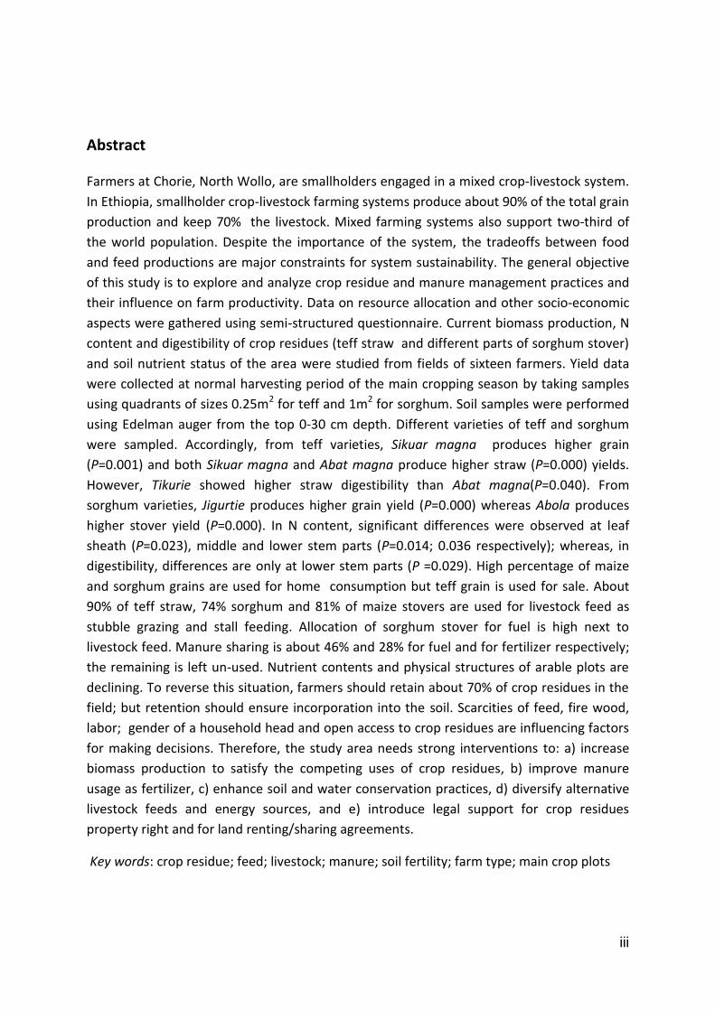
Farmers at Chorie, North Wollo, are smallholders engaged in a mixed crop-livestock system.
In Ethiopia, smallholder crop-livestock farming systems produce about 90% of the total grain
production and keep 70% the livestock. Mixed farming systems also support two-third of
the world population. Despite the importance of the system, the tradeoffs between food
and feed productions are major constraints for system sustainability. The general objective
of this study is to explore and analyze crop residue and manure management practices and
their influence on farm productivity. Data on resource allocation and other socio-economic
aspects were gathered using semi-structured questionnaire. Current biomass production, N
content and digestibility of crop residues (teff straw and different parts of sorghum stover)
and soil nutrient status of the area were studied from fields of sixteen farmers. Yield data
were collected at normal harvesting period of the main cropping season by taking samples
using quadrants of sizes 0.25m2 for teff and 1m2 for sorghum. Soil samples were performed
using Edelman auger from the top 0-30 cm depth. Different varieties of teff and sorghum
were sampled. Accordingly, from teff varieties, Sikuar magna produces higher grain
(P=0.001) and both Sikuar magna and Abat magna produce higher straw (P=0.000) yields.
However, Tikurie showed higher straw digestibility than Abat magna(P=0.040). From
sorghum varieties, Jigurtie produces higher grain yield (P=0.000) whereas Abola produces
higher stover yield (P=0.000). In N content, significant differences were observed at leaf
sheath (P=0.023), middle and lower stem parts (P=0.014; 0.036 respectively); whereas, in
digestibility, differences are only at lower stem parts (P =0.029). High percentage of maize
and sorghum grains are used for home consumption but teff grain is used for sale. About
90% of teff straw, 74% sorghum and 81% of maize stovers are used for livestock feed as
stubble grazing and stall feeding. Allocation of sorghum stover for fuel is high next to
livestock feed. Manure sharing is about 46% and 28% for fuel and for fertilizer respectively;
the remaining is left un-used. Nutrient contents and physical structures of arable plots are
declining. To reverse this situation, farmers should retain about 70% of crop residues in the
field; but retention should ensure incorporation into the soil. Scarcities of feed, fire wood,
labor; gender of a household head and open access to crop residues are influencing factors
for making decisions. Therefore, the study area needs strong interventions to: a) increase
biomass production to satisfy the competing uses of crop residues, b) improve manure
usage as fertilizer, c) enhance soil and water conservation practices, d) diversify alternative
livestock feeds and energy sources, and e) introduce legal support for crop residues
property right and for land renting/sharing agreements.
Key words: crop residue; feed; livestock; manure; soil fertility; farm type; main crop plots

iv
v
Table of contents
Dedication ...................................................................................................... i
Acknowledgement ......................................................................................... ii
Abstract ........................................................................................................ iii
List of Figures ...............................................................................................viii
List of Tables .................................................................................................. x
Abbreviations ............................................................................................... xi
Chapter 1. Introduction .................................................................................. 1
1.1 Background information.......................................................................................... 1
1.2 Research questions ................................................................................................. 3
1.3 Objectives ............................................................................................................... 3
Chapter 2. Literature review .......................................................................... 5
2.1 Role of crop residues as livestock feed .................................................................... 5
2.2 Crop residue allocation and trade-offs ..................................................................... 5
2.3 Method of crop residue application/retention ......................................................... 7
2.4 Effect of manure management strategies to whole farm nutrient flow .................... 8
Chapter 3. Methodology .............................................................................. 11
3.1 Study area selection .............................................................................................. 11
3.2 Farmer selection ................................................................................................... 11
3.3 Plant sampling and analysis ................................................................................... 12
3.4 Soil sampling and analysis ..................................................................................... 13
3.5 Model initialization and scenario analysis .............................................................. 13
3.6 Socio-economic data collection ............................................................................. 14
3.7 Data analysis and presentation of results .............................................................. 15
Chapter 4. Results ........................................................................................ 17
4.1 Characterization of farming system ....................................................................... 17
4.1.1 Herd characteristics ............................................................................................................ 17
4.1.2 Land holding ........................................................................................................................ 17
4.1.3 Gender of the household head ........................................................................................... 18
4.1.4 Household head literacy level ............................................................................................. 19
vi
4.1.5 Age characteristics .............................................................................................................. 19
4.1.6 Labor availability ................................................................................................................. 20
4.1.7 Land preparation and fertility management ...................................................................... 21
4.1.8 Crop types and land allocation ........................................................................................... 23
4.1.9 Food self sufficiency ............................................................................................................ 24
4.2 Quantity and quality of biomass production .......................................................... 25
4.2.1 Teff biomass production ..................................................................................................... 25
4.2.2 Sorghum biomass production ............................................................................................. 27
4.2.3 Nitrogen content and digestibility of teff straw .................................................................. 30
4.2.4 Teff grain nutrient content .................................................................................................. 31
4.2.5 Nitrogen content and digestibility of sorghum stover ........................................................ 32
4.2.6 Sorghum grain nutrient content ......................................................................................... 34
4.3 Resource allocation ............................................................................................... 35
4.3.1 Grain allocation ................................................................................................................... 35
4.3.2 Crop residue allocation ....................................................................................................... 35
4.3.3 Crop residue feeding strategy ............................................................................................. 37
4.3.4 Manure allocation ............................................................................................................... 40
4.4 Farmers’ decision-making on resources and limiting factors................................... 40
4.4.1 Decision maker .................................................................................................................... 40
4.4.2 Factors influencing decision making processes .................................................................. 41
4.4.2.1 Water availability ....................................................................................................................... 41
4.4.2.2 Land and herd size ...................................................................................................................... 42
4.4.2.3 Labor scarcity ............................................................................................................................. 42
4.4.2.4 Feed shortage ............................................................................................................................. 42
4.4.2.5 Gender of a house hold head ..................................................................................................... 43
4.4.2.6 Open access to crop residue ...................................................................................................... 44
4.4.2.7 Energy demand .......................................................................................................................... 44
4.4.2.8 Others ......................................................................................................................................... 45
4.5 Soil fertility ............................................................................................................ 45
4.5.1 Current fertility status ......................................................................................................... 45
4.5.2 Future trends in soil organic carbon and land productivity ................................................ 48
Chapter 5. Discussion ................................................................................... 53
5.1 Crop residues utilization ........................................................................................ 53
5.2 Manure utilization ................................................................................................ 54
5.3 Crop residues and manure management practices of farm types ........................... 55
5.4 Limitation of the study .......................................................................................... 56
Chapter 6. Conclusion and recommendation................................................ 57
List of references ......................................................................................... 59
Annexes ....................................................................................................... 63

vii
Annex 1. Population and land availability at Chorie village .......................................... 63
Annex 2. Parameters used to calibrate the model FIELD .............................................. 63
Annex 3. Questionnaire used for socio-economic data collection ................................. 65
Annex 4. Characteristics of teff and sorghum varieties ................................................ 74
Annex 5. Farmers’ saving strategy .............................................................................. 74
Annex 6. Decision makers on resources ...................................................................... 75
Annex 7. Number of days to mature for different crop types ....................................... 76
Annex 8: ANOVA for soil nutrient analysis of different farm types ............................... 76
viii
List of Figures
Figure 1. Geographical location of the study area ------------------------------------------------------11
Figure 2. Average herd and land size owned by different farm types------------------------------12
Figure 3. Fitness of the Model FIELD against measured and predicted yields--------------------13
Figure 4. Total herd size in TLU and in average number for different farm types --------------17
Figure 5. Average land holding of different farm types ----------------------------------------------18
Figure 6. Gender of a household head in different farm types--------------------------------------18
Figure 7. Literacy level of household heads and leading females in different farm types ----19
Figure 8. Average age of household heads and their years in the village ------------------------20
Figure 9. Average number of family members with different labor inputs -----------------------21
Figure 10. Seed bed preparation for different crops --------------------------------------------------22
Figure 11. Manure management practices by different farm types--------------------------------22
Figure 12. Average land allocation for different crops by farm types -----------------------------23
Figure 13. Teff varieties and their area coverage -------------------------------------------------------23
Figure 14. Sorghum varieties and their area coverage -----------------------------------------------24
Figure 15. Yield performance of different teff varieties ----------------------------------------------26
Figure 16. Correlation between measured and farmers' estimation of teff yields -------------26
Figure 17. Teff yields: measured vs. farmers' estimation---------------------------------------------27
Figure 18. Yield performance of sorghum varieties ----------------------------------------------------28
Figure 19. Quantity and proportion of parts of sorghum stover -----------------------------------28
Figure 20. Sorghum yields: measured vs. farmers' estimation---------------------------------------29
Figure 21. Correlation between measured and farmers' estimation of sorghum yields ------29
Figure 22. Teff grain and flour before and after scanning --------------------------------------------31
Figure 23. Protein, fat and starch content of teff varieties before and after grinding---------31
Figure 24. Grain nutrient content of sorghum varieties----------------------------------------------35
Figure 25. Grain allocation of different crops by farm types-----------------------------------------35
Figure 26. Estimation of teff straw allocation by farm types-----------------------------------------36
Figure 27. Estimation of sorghum stover allocation by farm types---------------------------------36
Figure 28. Estimation of maize stover allocation by farm types-------------------------------------37
Figure 29. Graph showing severity of dry feed shortage from grazing areas --------------------38
Figure 30. Stall feeding strategy from stored teff straw and sorghum stover -------------------38
Figure 31. Graph showing severity of green feed shortage ------------------------------------------39
Figure 32. Teff straw and sorghum stover heaps at home stead -----------------------------------39
Figure 33. Proportion of manure allocation to different uses by farm types---------------------40
Figure 34. Decision makers on resources -----------------------------------------------------------------41
Figure 35. Water purchasing for livestock consumption ----------------------------------------------42
Figure 36. Feed sources for livestock in different seasons -------------------------------------------43
ix
Figure 37. A poorly managed plot: owned by female headed household but shared----------43
Figure 38. Livestock freely grazing on previous cropped lands --------------------------------------44
Figure 39. Crop residue collection for fuel----------------------------------------------------------------44
Figure 40. Backing Injera using sorghum stover --------------------------------------------------------44
Figure 41. Dry dung collected from crop plots: for house use fuel----------------------------------44
Figure 42. Soil erosion, gully formation and farmer’s effort to protect soil erosion -----------47
Figure 43. Proportion of arable plots on the basis of SOC content ---------------------------------48
Figure 44. Simulation result of SOC for 3 scenarios based on soil types --------------------------49
Figure 45. Simulation result of above ground sorghum biomass for 3 scenarios based on soil
types----------------------------------------------------------------------------------------------------------------49
Figure 46. Simulation results of SOC for 3 scenarios based on farm types -----------------------50
Figure 47. Simulation results of above ground sorghum biomass for 3 scenarios based on
farm types---------------------------------------------------------------------------------------------------------51
x
List of Tables
Table 1. Soil parameters changed to adapt the model FIELD----------------------------------------14
Table 2. Different scenarios used to simulate above ground biomass and SOC-----------------14
Table 3. Reasons for labor shortage and strategies used by farm types to solve it-------------21
Table 4. Average cereal food self-sufficiency and food aid received years in last 10 years---24
Table 5. Percentage of food remedial sources at scarcity periods (%) ----------------------------25
Table 6. ANOVA Table for grain and straw yields of teff varieties-----------------------------------25
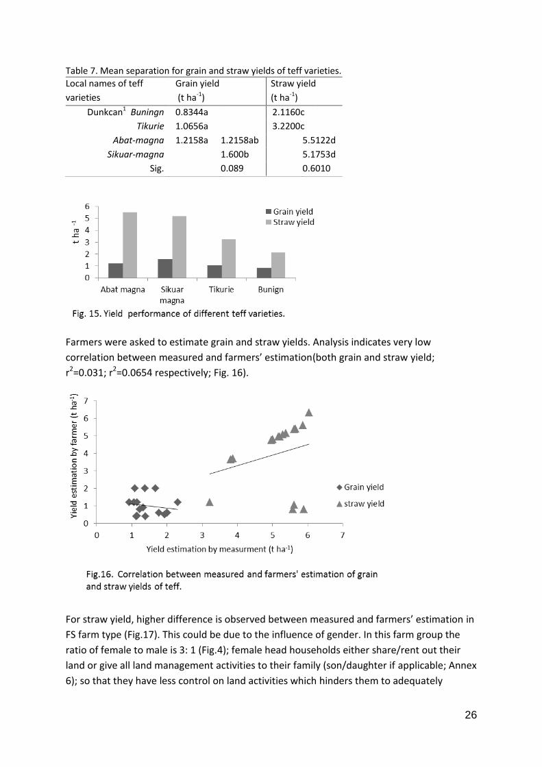
Table 7. Mean separation for grain and straw yields of teff varieties -----------------------------26
Table 8. ANOVA Table for grain and stover yields of sorghum varieties---------------------------27
Table 9. Mean separation for grain and stover yields of sorghum varieties ---------------------28
Table 10. ANOVA Table for nitrogen content and straw digestibility of teff varieties---------30
Table 11. Mean separation for straw digestibility of teff varieties ---------------------------------30
Table 12. ANOVA Table for N content and digestibility of sorghum leaf sheaths ---------------32
Table 13. ANOVA Table for N content and digestibility of middle stems of sorghum ---------32
Table 14. ANOVA Table for N content and digestibility of lower stems of sorghum------------33
Table 15. N content (%-dm) and digestibility of lower stems of sorghum varieties------------33
Table 16. N content (%-dm) of different stover parts of Jigurtie------------------------------------34
Table 17. Digestibility (Invomd%) of different stover parts of Jigurtie-----------------------------34
Table 18. Influencing factors in making decisions: ranks according to farmers’ priority-------42
Table 19. ANOVA Table for soil nutrient contents of different crops’ fields----------------------46
Table 20. Mean separation for soils of different crop fields in nutrient content----------------46
Table 21. Soil organic carbon (SOC)of arable plots -----------------------------------------------------48
xi
Abbreviations
AfricaNUANCES Nutrient Use in Animal and Crop systems-Efficiencies and Scales
ANOVA Analysis of variance
C carbon
CEC Cation exchange capacity
CROPSIM Crop production SIMulator
dm dry matter
FIELD Field scale resource Interactions, use Efficiencies and Long term soil fertility
Development
Fig. Figure
Figs Figures
FL farmer group that have Fewer livestock and Larger crop lands
FS farmer group that have Fewer livestock and Smaller crop lands
ha hectare
ILRI International Livestock Research Institute
Ivomd Invitro organic matter digestibility
K potassium
kg Kill gram
km kilo meters
LSD Least Significant Difference
masl meters above sea level
MATLB MATrix LaBoratory (a numerical computing environment and fourth-generation
programming language)
ME metabolizable energy
Mj Mega joule
ML farmer group that have More livestock and Larger crop lands
mm millimeter
MS farmer group that have More livestock and Smaller crop lands
N nitrogen
N-dm% nitrogen content on percent dry mater basis
NIRS Near Infrared Reflectance Spectroscopy oC degree Celsius
P phosphorus
PH Scale used to measure acidity and alkalinity
Ppm Parts per million
RF Rain fall
SLP System-wide Livestock Program
SOC soil organic carbon

xii
TLU Tropical Livestock Units

xiii

xiv
1
Chapter 1. Introduction
1.1 Background information
Farmers at Chorie, North Wollo, are smallholders engaged in a mixed crop-livestock system.
Small holder crop-livestock systems are dominant in Ethiopia. In the country, these systems
produce about 90% of the total grain production (Anderson, 1987; Jagtap and Amissah,
1999) and keep about 70% of the livestock (Shitahun, 2009). One can see the potential of
this smallholder crop-livestock integrated farming to provide food and feed to peoples’
livelihood in the country. The systems also play significant role in other parts of the
developing world. According to Herrero et al. (2010), mixed crop-livestock farming systems
support the world’s 1 billion poor people; they reported that two-third (2/3) of the global
population live in small holder crop-livestock systems.
Crop-livestock integrated farming is complex and dynamic with many interacting biophysical
resources (Mark et al., 2009) and socio-economic factors. Productivity and sustainability of
a system depends on appropriate decisions on resource allocations on to the different
sectors and efficient use of available resources. Key resources that can form constraints for
crop-livestock systems include land, livestock, feed, labor, soil nutrients, cash and market
(Giller et al., 2006; 2009). Decisions on these resources are influenced by a number of
factors such as rainfall, tenure security, household endowments (Di Falco et al., 2010),
gender, as well as short term and long term needs of households. Since the most
responsible person to make decision is the head of the household, gender of the head of the
household is an important factor for resource allocation.
In the study area, Chorie, there are households headed by different genders (male or
female). Males are the dominant decision makers on land management activities, selection
of crop varieties, management of crop residues and livestock activities. Females in male
headed households do not make decision independently; sometimes they decide jointly
with their husband. Female headed households depend on decisions of family members
(son/daughter if available) or land tillers/shareholders. When female headed households
rent out their crop land, the renter do not worry about fertility management of rented plots
aiming at short-term benefits. Likewise, lands given for share are managed after all land
activities are performed for the private plots so that there is a delay in the timing of land
preparation, weeding and harvesting activities for the shared plots. Delayed land activities
also influence the type of crop to be planted which determines the yield at the end. As a
result of these, productivity and sustainability of rented/shared plots is at risk.
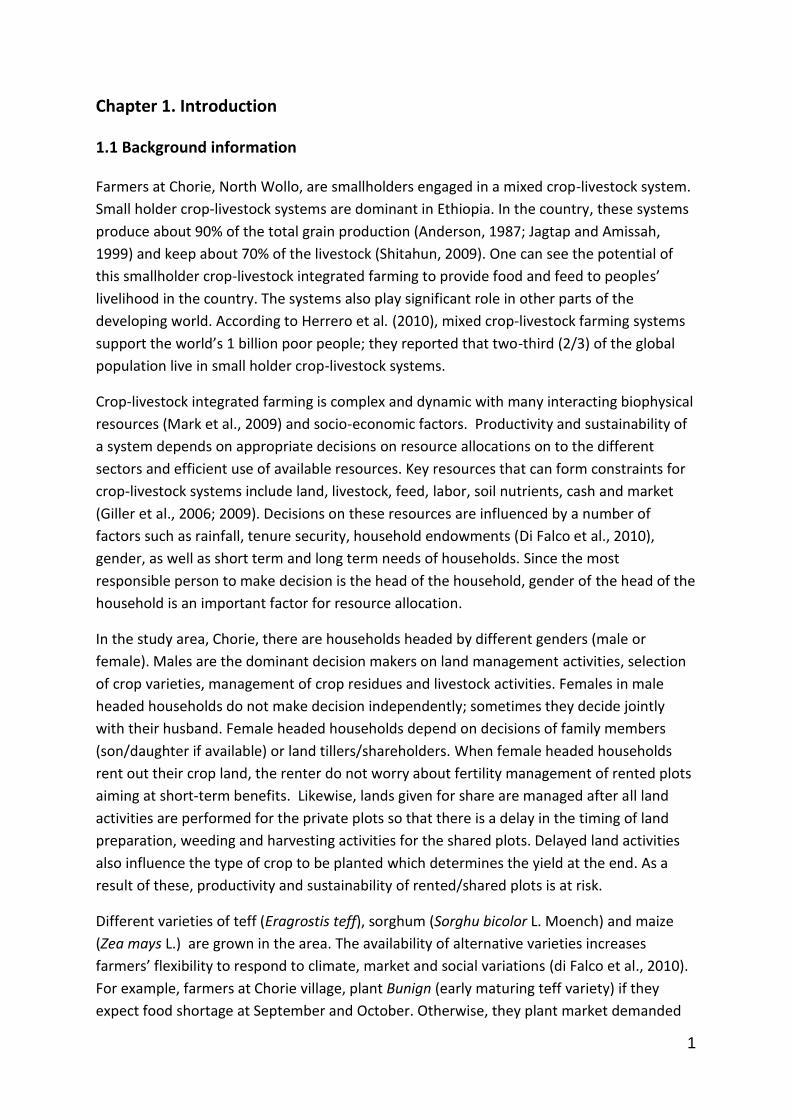
Different varieties of teff (Eragrostis teff), sorghum (Sorghu bicolor L. Moench) and maize
(Zea mays L.) are grown in the area. The availability of alternative varieties increases
farmers’ flexibility to respond to climate, market and social variations (di Falco et al., 2010).
For example, farmers at Chorie village, plant Bunign (early maturing teff variety) if they
expect food shortage at September and October. Otherwise, they plant market demanded
2
variety “Sikuar magna”. Variety selection for sorghum depends on rain fall. High yielding
varieties (Abola and Jigurtie) require longer periods to mature. They can be planted if there
is sufficient rain in April and May. The low yielding but early maturing variety Wedhakir is
used as an alternative if there is failure of rain in these months. Mostly, teff grain is used for
sale whereas, sorghum and maize grains are used for home consumption. Residues from
both teff, sorghum and maize crops are mainly used for livestock feed. Moreover, sorghum
stover is also used as energy source for cooking in the house.
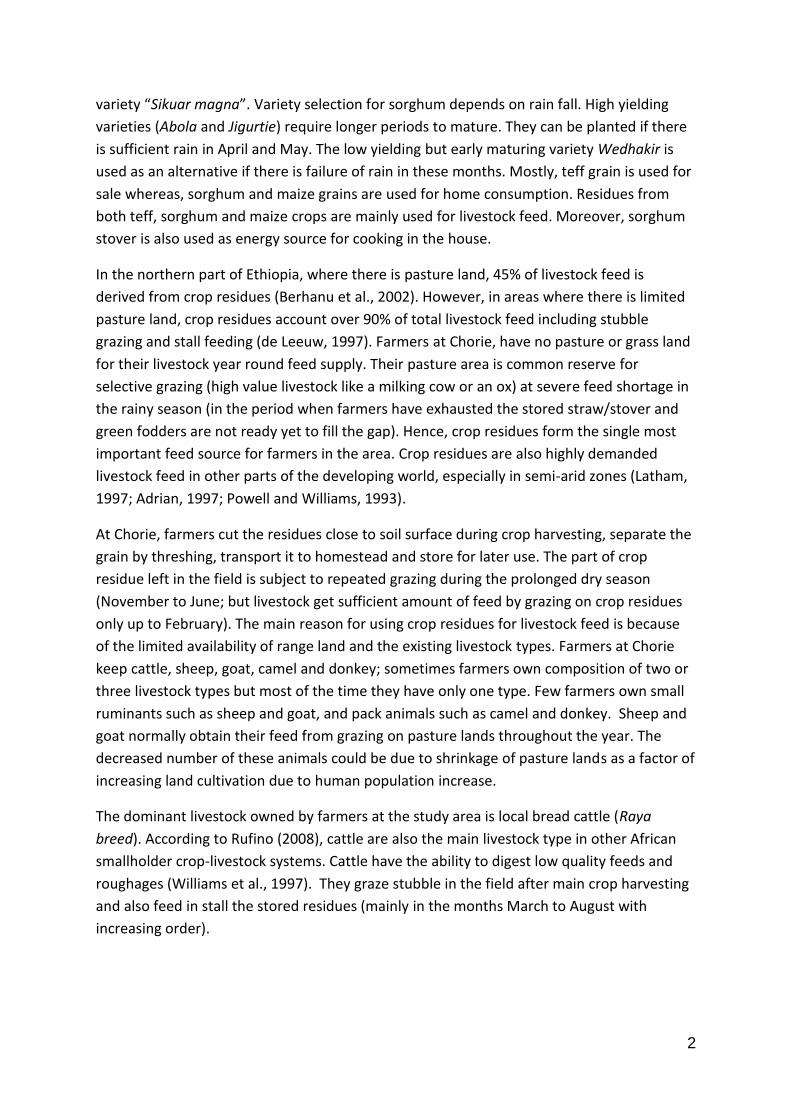
In the northern part of Ethiopia, where there is pasture land, 45% of livestock feed is
derived from crop residues (Berhanu et al., 2002). However, in areas where there is limited
pasture land, crop residues account over 90% of total livestock feed including stubble
grazing and stall feeding (de Leeuw, 1997). Farmers at Chorie, have no pasture or grass land
for their livestock year round feed supply. Their pasture area is common reserve for
selective grazing (high value livestock like a milking cow or an ox) at severe feed shortage in
the rainy season (in the period when farmers have exhausted the stored straw/stover and
green fodders are not ready yet to fill the gap). Hence, crop residues form the single most
important feed source for farmers in the area. Crop residues are also highly demanded
livestock feed in other parts of the developing world, especially in semi-arid zones (Latham,
1997; Adrian, 1997; Powell and Williams, 1993).
At Chorie, farmers cut the residues close to soil surface during crop harvesting, separate the
grain by threshing, transport it to homestead and store for later use. The part of crop
residue left in the field is subject to repeated grazing during the prolonged dry season
(November to June; but livestock get sufficient amount of feed by grazing on crop residues
only up to February). The main reason for using crop residues for livestock feed is because
of the limited availability of range land and the existing livestock types. Farmers at Chorie
keep cattle, sheep, goat, camel and donkey; sometimes farmers own composition of two or
three livestock types but most of the time they have only one type. Few farmers own small
ruminants such as sheep and goat, and pack animals such as camel and donkey. Sheep and
goat normally obtain their feed from grazing on pasture lands throughout the year. The
decreased number of these animals could be due to shrinkage of pasture lands as a factor of
increasing land cultivation due to human population increase.
The dominant livestock owned by farmers at the study area is local bread cattle (Raya
breed). According to Rufino (2008), cattle are also the main livestock type in other African
smallholder crop-livestock systems. Cattle have the ability to digest low quality feeds and
roughages (Williams et al., 1997). They graze stubble in the field after main crop harvesting
and also feed in stall the stored residues (mainly in the months March to August with
increasing order).
3
This research is part of the SLP-ILRI (System wide Livestock Program- International Livestock
Research Institute) research project entitled “Optimizing livelihood and environmental
benefits from crop residues in smallholder crop-livestock systems in sub-Saharan Africa and
South Asia: regional case studies”. In Africa the project conducts research at South Africa,
West Africa and East Africa. Kenya and Ethiopia are the East Africa countries for the project.
In Ethiopia there are two sites: Nekemte (western Ethiopia) and Kobo (North-Eastern
Ethiopia); at each site eight villages are selected. This thesis explores farming system at
Chorie village, one of the eight selected villages at Kobo site. The village is one of the two
near-near (near to market- near to road access) villages. In the village, farmers settled on
higher slopes following the contour of the mountain. Their main arable plots are far from
home. Majority of the farmers own less than 1.5 ha of land.
In the study area, farmers depend on crop residues for their livestock feed through direct
grazing in the field and in stall after livestock clear stubbles and when crop lands are
planted. However, they do not apply soil fertility inputs such as manure or chemical fertilizer
to the main arable plots. In crop-livestock farming, nutrient cycling of crop residues in to
manure (Harris 2002; Zingore et al., 2007a; Samaddar, 2008) governs system sustainability
but farmers in the study area do not sufficiently use manure for soils while they total
depend on crop residue for their livestock feed. Furthermore, they use sorghum stover as
energy source for cooking. This practice without soil amendment strategies resulted in
severe soil fertility degradation. This report presents investigation of current biomass
production and crop residue and manure management practices of farmers at Chorie
village, North Wollo, Ethiopia. Furthermore, it describes factors that are influencing farmers’
decisions, and indicates the long-term impacts of current practices on soil fertility and land
productivity status.
1.2 Research questions
1. How important are crop residues and manure for farm productivity in smallholder
crop-livestock system?
2. What is the current crop residue and manure management practice of farmers at
Chorie village? Are there differences among farm types or not?
3. What are influencing factors for farmers’ decisions on resource allocation?
4. How important is the influence of current crop residue and manure management
practices on future land productivity?
1.3 Objectives
General objective:- the general objective of this research is to explore and analyze how crop
residues and manure management practices influence farm productivity in smallholder
crop-livestock farming systems.

4
Specific objectives:-the specific objectives of this research are:
To review literatures on the role of crop residues and manure in a mixed farming
system
To characterize the farming system (crops and livestock) of Chorie village
To quantify biomass production, analyze N content and digestibility of crop residues
To understand farmers’ resource allocation, decision making processes and
influencing factors for decision makings
To assess long-term impact of crop residues and manure management practices on
land productivity
5
Chapter 2. Literature review
2.1 Role of crop residues as livestock feed
According to Zingore et al. (2007a), livestock have multiple functions in the economy of
smallholder farms in sub-Saharan Africa. To mention few of the benefits, they are major
capital investment, play significant role in food security through products such as milk and
meat; they provide labor for land cultivation and threshing, and they add nutrients to soils
through manure (Tangka et al., 2000; Herrero et al., 2010). Furthermore, livestock play
significant role in recycling nutrients from pasture lands and grazing stubbles to arable plots.
The economic and social values of livestock ensure their importance in the mixed
production system. However, feed shortage due to land use changes from grazing/pasture
lands to crop lands caused by population growth (Anderson, 1987; Berhanu et al, 2002;
Harris, 2002; Ebanyat et al., 2010) limits the number and type of livestock. The problem
forced farmers to shift their feeding strategy from pasture/range source to crop residues.
Crop residues are considered as by-products in crop production activities but they are vital
source of livestock feed in the mixed crop-livestock system (Williams et al., 1997). Crops
provide residues (straws/stover) and un-marketable surpluses to feed livestock. This role
may not be significant in places where there is range land that livestock can get considerable
amount of feed. However, since crop-livestock farming system is historically created due to
increased human populations (Harris, 2002), in the process, range lands are converted to
crop lands; and thus, major feed sources for livestock are becoming crop by-products such
as the residues. Livestock, especially large ruminants, convert these materials into high
value products: milk and meat for human consumption and dung/manure which can be
returned back to the soil. Nevertheless, over use of crop residues for livestock feed could
result in declining productivity of the farm due to extreme nutrient export from arable plots.
Strategies to ensure sustainable productivity of mixed crop-livestock systems should focus
on balancing the flow of nutrients between the crop and livestock sectors (Tittonell et al.,
2008; Benjamin et al., 2010). This can be done by efficient use of manure for soil fertility
management, substantial amount of crop residue retention in the field and additional inputs
from outside of the field to replenish nutrients that are lost in the process. Maintaining soil
fertility guarantees good crop biomass production and sustainable crop residues supply for
livestock; hence sustaining the nutrient flow.
2.2 Crop residue allocation and trade-offs
Poor soil organic matter content and limited nutrient availability to crops are key problems
to low agricultural productivity of sub-Saharan Africa (Schlecht and Hiernaux, 2004). The
physical, chemical and biological properties of soils can be improved through addition of
6
organic materials (Waswa et al., 2007). The level of organic matter or carbon in agricultural
soils depends on additions from crop residues and manure, and losses from erosion and
decomposition (Beauchamp and Voroney, 1994). Benjamin et al. (2010) identified that crops
that produce more residues have greater potential for increasing soil organic carbon than
crops which produce low crop residues. The finding is in line with Tittonell et al. (2008).
According to their report carbon supply to soils is a factor of biomass yields, harvest index
and the proportion of feed carbon retained in the manure. In crop-livestock mixed system
where there is high percentage of crop residue allocation for feed, soil C maintenance is
only from manure and root-C inputs.
Besides livestock feed and other uses like construction materials and energy supply, crop
residues are extremely important to soils to improve its chemical and physical
characteristics. They enhance soil structure, reduce soil erosion and improve water
availability to plants (Latham, 1997; Tittonell et al., 2008). The work done by Hartkamp et al.
(2004) in Mexico revealed that retention of small amount of crop residues (1.5t ha-1)
doubled maize yield even at low rain fall areas. The result shows 40% increase in soil water
content whereas 50% and 80% decrease in surface and soil particles run off respectively.
Crop residues are also nutrient sources for soil fertility improvement. Crop residues
represent about half of the nutrients exported through the main commodity production
(Unger 1990, cited in Latham, 1997). Therefore, substantial amounts of crop residue
retention increase soil fertility. The effect is high when combined with other nutrient
sources like manure or inorganic fertilizer (Aggarwal et al., 1997). Addition of crop residues
and farm yard manure improved N and P availability, soil water availability, soil organic
matter content and enzyme activity compared to no residue treatments. Furthermore, their
study showed higher mineral fertilizer use efficiency for crop residue applied plots. This soil
fertility enhancement increased grain and straw yields.
The research done by Tittonell et al. (2008) also confirmed the importance of crop residues
to increase fertilizer use efficiency in soil nutrient restoration activities. Application of basal
fertilizer rate maintained initial soil C content on fertile fields where 70% of crop residues
were retained. This was not possible on fields where 10% of crop residues were maintained.
From these findings, one can appreciate the role of crop residues in sustaining soil fertility
and productivity. However, Aggarwal et al. (1997) reported that the benefit from crop
residues and manure in tropical regions may not be as evident as for temperate regions
because of rapid oxidation in the area. Yet, crop residues are basic components of a number
of agronomic technologies.
Effective soil and water conservation practices are possible when crop residues are
adequately available (Unger et al., 1991; 1997). In dry land areas moisture and soil
characteristics are major production limiting factors. Since crop residues have the potential
to reduce soil degradation and improve water infiltration, they can be used as a strategic
intervention to improve land productivity through effective soil and water conservation
7
practices. Thus, crop residue allocation for livestock feed and for soil fertility measures are
key management aspects to avoid negative trade-offs between the livestock and crop
sectors in crop-livestock systems.
There are different ways of balancing the trade-offs. Unger et al. (1997) suggested
alternative crop residue management practices such as: 1) selective residue removal, 2)
substituting crop residues to animal feed by high quality forages, 3) practicing alley cropping
of nitrogen fixing plants at field margins/hedges, 4) more effective use of waste lands, 5)
improving the balance between feed supplies and animal populations, and 6) using
alternative fuel sources. These alternatives require inter-disciplinary and integrated
approaches based on realities existing under local circumstances. The extent of feed
shortage and or seasonal biomass production determines degree of selective residue
removal from fields. Technology availability, accessibility, land size and tenure system may
be the frontier bottlenecks to substitute crop residues with high quality livestock feed and
so on. However, the farming system cannot be sustainable unless farmers are determinant
to allocate appropriate amount of crop residues and manure and other fertilizers to improve
the fertility of their soils (Benjamin et al., 2010).
Therefore, exhausting local resources and synthesizing situations from different point of
views are needed to design the best appropriate technological combinations to improve
allocation of crop residues for various needs. Single technology may not solve crop residue
trade-offs; equally important is the fit of technologies to farming system (Rufino, 2008).
2.3 Method of crop residue application/retention
Different views are reported on the method of crop residue retention practices: direct
application on the soil (Samaddar et al., 2008) and application after composting (Abegaz et
al., 2007). Abegaz et al. (2007) argue that the C:N ratio of crop residues is high and direct
application can result in negative effect on soil productivity due to N immobilization during
the process of decomposition. However, composting requires labor for collecting,
preparation of peats and re-distribution. It is unlike that composts will be evenly distributed
throughout crop fields as the practice of farmers is evident in manure application (Zingore
et al., 2007b). Hence, composting crop residues and re-distribution may result in nutrient
gradients such that more nutrients near to compost peats and less nutrients to marginal
fields. On the other hand crop residue retention alone may not ensure soil organic matter
supply because; in some places they might be exposed to wind erosion, communal grazing
and or free collection for fuel in addition to N immobilization. This needs a practice that
ensures even distribution and proper incorporation of crop residues in the soil.
One way to do this may be burring crop residues by early tillage. In Ethiopian farming, tillage
operation is done mostly after crop residues are cleared from arable plots and when rainy
months are approaching with the objective to increase water infiltration and storage
through trapping run off and reducing evaporation (Temesgen et al., 2008). In the study
8
area there is no tillage schedule to incorporate residues in to the soil. Having many research
findings on the role of crop residue retention in improving soil nutrients and physical
characteristics, can residue retention alone ensure their availability as an organic input to
the soil? To what extent are retained residues incorporated in to the soil?
Zeleke et al. (2004) reported that incorporation of crop residues by tillage operation
improved rain water use efficiency and soil tilth. Since crop residues are vulnerable for free
grazing and collection to fuel, at Chorie, tillage need to be scheduled as early as possible
before they disappear from the farm. Early tillage operation following crop harvest may trap
residues at the place where they are produced. The practice could give more benefit to
farmers that have few or no livestock than those who have more livestock. Since nutrients
are freely exported from poor farmers and accumulated to rich farmers who own more
livestock through free grazing, farmers who have no or few livestock are the losers in the
system. Hence, early tillage practice may give guarantee to poor farmers (who are unable to
buy fertilizer and do not have access to manure) to return nutrients back to their soil. Early
tillage also allows incorporation of weeds and grasses while they are relatively green which
probably have better benefit than their effect after drying. It becomes apparent that early
tillage still have negative trade-offs for livestock feed from stubble grazing. However, it may
also influence farmers to limit the number of livestock to available resources and avoid over
exploitation of nutrients and environment degradation as a factor of competition for
communal resources.
2.4 Effect of manure management strategies to whole farm nutrient flow
Cycling of biomass through livestock excreta is an important linkage between livestock and
soil productivity (Powel and Williams, 1993; Rufino, 2008) in crop-livestock mixed farming
system. Manure is a corner stone to improve the chemical and physical characteristics of
soils in smallholder crop-livestock integrated systems (Harris, 2002). Manure can improve
soil pH, cation exchange capacity, water holding capacity, and soil structure. Nutrients from
manure are released slowly over the growing season and have residual effect to the next
crop. Studies reveal that farmers in sub-Saharan Africa have the knowledge about the role
of manure in supplying nutrients to soils and improving its fertility, but they lack sufficient
quantity to cover all of their plots and labor to distribute over fields. Manure production can
be increased by increasing herd size, but this is not possible for the current smallholder
farmers because of droughts (Zingore et al., 2007a) and feed shortage due to range land
shrinkage (Ebanyat et al., 2010). Manure application is therefore concentrated around
homesteads as a result of small quantity to cover all plots and labor constraints for
distribution.
Farmers in the study area do not apply manure to their main arable plots. This could be
influenced by their settlement location which creates inconveniencies to transport manure
and lack of knowledge regarding manure management and uses. Villagers live following a
9
raised mountain belt far from their main crop plots. Previous studies reported that farmers
apply more manure and other organic inputs on close to home plots than on distant plots
(Zingore, 2006; Zingore et al., 2007a; b; Bationo et al., 2007; Okumu et al., 2011). As a result
of this preferential land management, soil fertility decline was observed as plots are more
distant from the homesteads. However, it is not only the physical distribution of manure
that matters, but also low quality in its nutrient content can create low effect in improving
soil fertility.
Manure storage and handling practice of smallholder farmers of sub-Saharan Africa is poor;
conditions that allow excessive aeration have high potential for ammonia loss (Powell and
Williams, 1993; Nzuma et al., 1997; Rufino, 2008). These researchers suggest developing
manure management options to minimize nutrient losses and enhance manure quality.
Rufino (2008) showed considerable reduction in manure mass and N losses by covering the
manure heap with polythene film. Farmers can use locally available covering materials or
shades to improve manure storage conditions. Farmers may be discouraged by their manure
application practice because of the weak effect of local manure in restoring the productivity
of degraded soils. However, combination of poor quality manure with small amount of
mineral fertilizer may give attractive response in the short term and more balanced build-up
of soil C and nutrient stock in the long term (Tittonell et al., 2008; Giller et al., 2011).

10
11
Chapter 3. Methodology
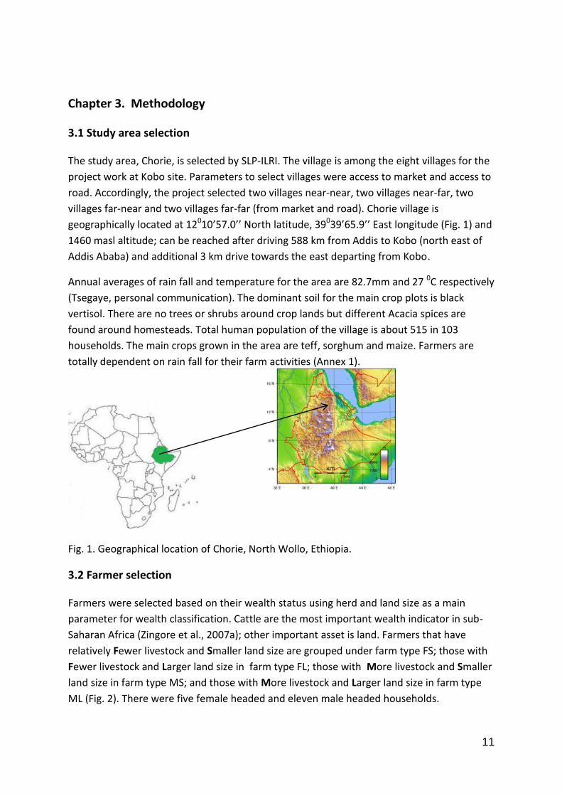
3.1 Study area selection
The study area, Chorie, is selected by SLP-ILRI. The village is among the eight villages for the
project work at Kobo site. Parameters to select villages were access to market and access to
road. Accordingly, the project selected two villages near-near, two villages near-far, two
villages far-near and two villages far-far (from market and road). Chorie village is
geographically located at 12010’57.0’’ North latitude, 39039’65.9’’ East longitude (Fig. 1) and
1460 masl altitude; can be reached after driving 588 km from Addis to Kobo (north east of
Addis Ababa) and additional 3 km drive towards the east departing from Kobo.
Annual averages of rain fall and temperature for the area are 82.7mm and 27 0C respectively
(Tsegaye, personal communication). The dominant soil for the main crop plots is black
vertisol. There are no trees or shrubs around crop lands but different Acacia spices are
found around homesteads. Total human population of the village is about 515 in 103
households. The main crops grown in the area are teff, sorghum and maize. Farmers are
totally dependent on rain fall for their farm activities (Annex 1).
Fig. 1. Geographical location of Chorie, North Wollo, Ethiopia.
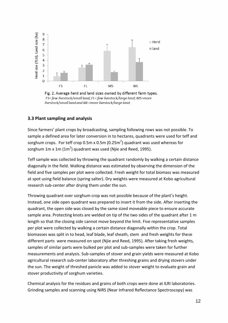
3.2 Farmer selection
Farmers were selected based on their wealth status using herd and land size as a main
parameter for wealth classification. Cattle are the most important wealth indicator in sub-
Saharan Africa (Zingore et al., 2007a); other important asset is land. Farmers that have
relatively Fewer livestock and Smaller land size are grouped under farm type FS; those with
Fewer livestock and Larger land size in farm type FL; those with More livestock and Smaller
land size in farm type MS; and those with More livestock and Larger land size in farm type
ML (Fig. 2). There were five female headed and eleven male headed households.
12
3.3 Plant sampling and analysis
Since farmers’ plant crops by broadcasting, sampling following rows was not possible. To
sample a defined area for later conversion in to hectares, quadrants were used for teff and
sorghum crops. For teff crop 0.5m x 0.5m (0.25m2) quadrant was used whereas for
sorghum 1m x 1m (1m2) quadrant was used (Njie and Reed, 1995).
Teff sample was collected by throwing the quadrant randomly by walking a certain distance
diagonally in the field. Walking distance was estimated by observing the dimension of the
field and five samples per plot were collected. Fresh weight for total biomass was measured
at spot using field balance (spring salter). Dry weights were measured at Kobo agricultural
research sub-center after drying them under the sun.
Throwing quadrant over sorghum crop was not possible because of the plant’s height.
Instead, one side open quadrant was prepared to insert it from the side. After inserting the
quadrant, the open side was closed by the same sized moveable piece to ensure accurate
sample area. Protecting knots are welded on tip of the two sides of the quadrant after 1 m
length so that the closing side cannot move beyond the limit. Five representative samples
per plot were collected by walking a certain distance diagonally within the crop. Total
biomasses was split in to head, leaf blade, leaf sheath, stem and fresh weights for these
different parts were measured on spot (Njie and Reed, 1995). After taking fresh weights,
samples of similar parts were bulked per plot and sub-samples were taken for further
measurements and analysis. Sub-samples of stover and grain yields were measured at Kobo
agricultural research sub-center laboratory after threshing grains and drying stovers under
the sun. The weight of threshed panicle was added to stover weight to evaluate grain and
stover productivity of sorghum varieties.
Chemical analysis for the residues and grains of both crops were done at ILRI laboratories.
Grinding samples and scanning using NIRS (Near Infrared Reflectance Spectroscopy) was
13
done at ILRI-Addis, Ethiopia; and NIRS results were sent to India for estimation of nutrient
contents using standard calibration models. “NIRS is an accepted method by international
standards committees to carry out many constituents of various tissues of many plants [...]
*including+ grains and fibers” (Batten, 1998). Samples were crushed to pass 1 mm sieve
(Njie and Reed, 1995), dried overnight at a temperature of 600C and filled in caps for
scanning by the NIRS machine.
NIRS results for teff and sorghum residues are estimated using mixed feed global calibration
model, teff grains (seed and flour) are predicted using millet grain and flour calibration
model, and sorghum grain (flour) is predicted using millet flour 195 calibration model (Jean,
personal communication).
3.4 Soil sampling and analysis
Soil samples were taken from all plots owned by the four farm types. The type of crop
grown on a plot was recorded during sampling. Sampling was performed using Edelman
auger from top 0-30 cm depth. Representative samples were taken from 3-5 points per plot
depending on the size and uniformity of plots. The collected samples were submitted to the
laboratory of national soil testing center, Addis Ababa, Ethiopia for pH, SOC, N, P and K
analysis.
3.5 Model initialization and scenario analysis
Long-term impact of the current crop residues and manure management practices on land
productivity and soil carbon stock is simulated using FIELD (Field scale resource Interactions,
use Efficiencies and Long term soil fertility Development), the CROPSIM (Crop production
SIMulator), in the AfricaNUANCES (Nutrient Use in Animal and Crop systems-Efficiencies and
Scales) framework. The model was parameterized for maize and extensively used in Kenya
and Zimbabwe. It was adapted to predict sorghum and pearl millet grain yields in Mali
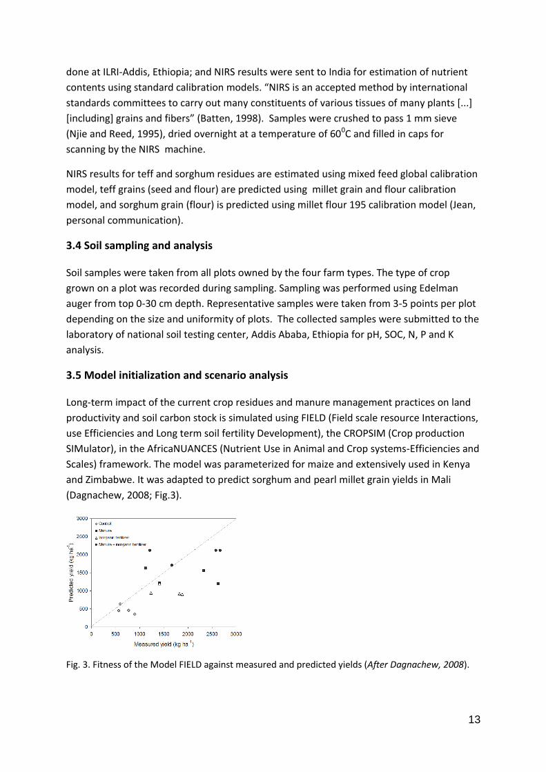
(Dagnachew, 2008; Fig.3).
Fig. 3. Fitness of the Model FIELD against measured and predicted yields (After Dagnachew, 2008).
14
Site, soil and crop specific parameters (Annex 2a-d) are used from Dagnachew thesis work
to initialize the model. After initializing the model, only rain fall and some soil parameters
of Chorie village are used to simulate future biomass production and soil carbon status of
the area. Parameters changed to adapt the model are seasonal rain fall (560 mm; Tsegaye,
personal communication) and soil parameters given below.
Table 1. Soil parameters changed to adapt the model, FIELD.
No. Description Remark
1. Soil texture (%) Values for each parameter are not given here; because, they differ as per the plots and farm types.
Clay Sand Silt
2. Soil organic carbon (g kg-1) 3. Total soil N (g kg-1) 8. CEC (cation exchange capacity) 9. PH
Three scenarios (Table 2) are simulated to see the impact of different levels of crop residue
retention on above ground sorghum biomass and soil carbon stock for 10 years. Farmers’
settlement location created considerable distance between main crop plots and homes;
because of this reason, manure application is not feasible for the time being; hence, no
scenario test is performed considering manure as soil amendment strategy. Besides, data
on quantity and quality of manure were not collected as per the model requirement.
Table 2. Different scenarios used to simulate above ground biomass
production and soil carbon stock for the next 10 years.
1. Fraction of residue removal.
3.6 Socio-economic data collection
Socio economic data (age, gender, literacy level, land and herd characteristics, crops and
area coverage, food self-sufficiency, resource allocation, decision making processes and
limiting factors) were collected by interviewing selected farmers(N=16) using semi-
structured questionnaire (Annex 3). Literacy level was determined by the number of study
years (formal or informal education system; 1 year =1 grade level). Land is quantified using
the local unit “timd” meaning one day plowing with a pair of oxen; and converting it in to
hectare (4 timds =1 ha). Type and number of livestock owned by each farmer is converted
to TLU (Tropical Livestock Units). Exploration of crop types and their area coverage was
done by constructing a resource flow map for each farmer during the interview. Resource
allocations such as grain, crop residue and manure were quantified using the five fingers of
Scenario FRREM1
1 1
2 0.7
3 0.3
15
a hand to make easy for farmers to estimate the proportion of their allocation; then values
were converted to percentages. Stall feeding of crop residues was estimated from the
amounts farmers gave to their livestock each day in each month of the year and converting
it to kilo grams and finally to percentage (according to farmers’ estimation 1 ekif crop
residue ≈ 5kg).
3.7 Data analysis and presentation of results
Socio-economic data are analyzed using Excel. Straw/stover and grain yields as well as
nutrient contents of these plant parts were analyzed using Excel and SPSS version 16
statistical software. Statistical differences between varieties and parts of a crop were
determined using Analysis of Variance (one way ANOVA procedure). Mean separations were
computed using LSD and Duncans’ homogeneity test at α= 0.01 and 0.05. MATLAB (MATrix
LaBoratory [a numerical computing environment and fourth-generation programming
language]) is used to run the simulation.
Results are presented in figures and tables with supportive explanation. Pictures taken at
the field during sampling are also used to illustrate some of the existing practices.

16
17
Chapter 4. Results
4.1 Characterization of farming system
4.1.1 Herd characteristics
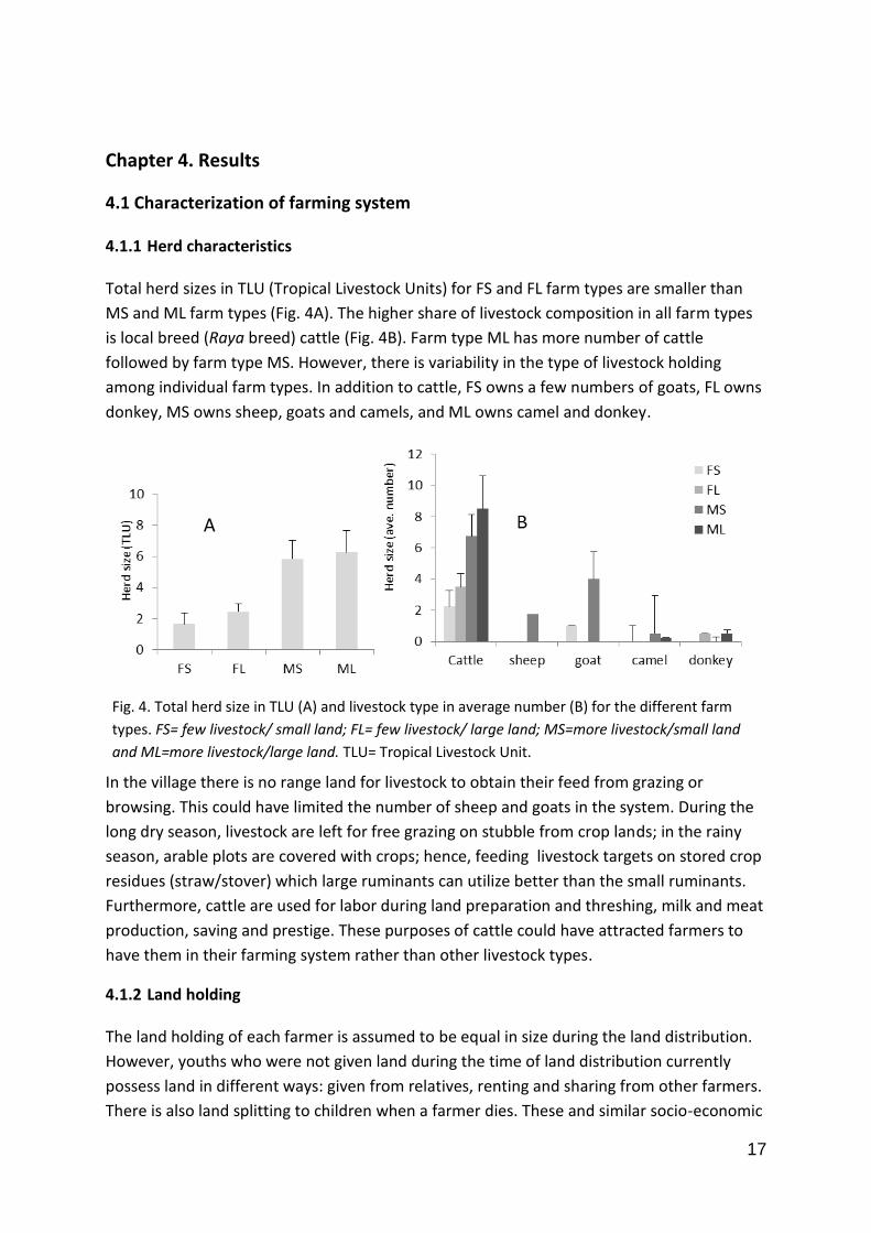
Total herd sizes in TLU (Tropical Livestock Units) for FS and FL farm types are smaller than
MS and ML farm types (Fig. 4A). The higher share of livestock composition in all farm types
is local breed (Raya breed) cattle (Fig. 4B). Farm type ML has more number of cattle
followed by farm type MS. However, there is variability in the type of livestock holding
among individual farm types. In addition to cattle, FS owns a few numbers of goats, FL owns
donkey, MS owns sheep, goats and camels, and ML owns camel and donkey.
In the village there is no range land for livestock to obtain their feed from grazing or
browsing. This could have limited the number of sheep and goats in the system. During the
long dry season, livestock are left for free grazing on stubble from crop lands; in the rainy
season, arable plots are covered with crops; hence, feeding livestock targets on stored crop
residues (straw/stover) which large ruminants can utilize better than the small ruminants.
Furthermore, cattle are used for labor during land preparation and threshing, milk and meat
production, saving and prestige. These purposes of cattle could have attracted farmers to
have them in their farming system rather than other livestock types.
4.1.2 Land holding
The land holding of each farmer is assumed to be equal in size during the land distribution.
However, youths who were not given land during the time of land distribution currently
possess land in different ways: given from relatives, renting and sharing from other farmers.
There is also land splitting to children when a farmer dies. These and similar socio-economic
Fig. 4. Total herd size in TLU (A) and livestock type in average number (B) for the different farm
types. FS= few livestock/ small land; FL= few livestock/ large land; MS=more livestock/small land
and ML=more livestock/large land. TLU= Tropical Livestock Unit.
A
18
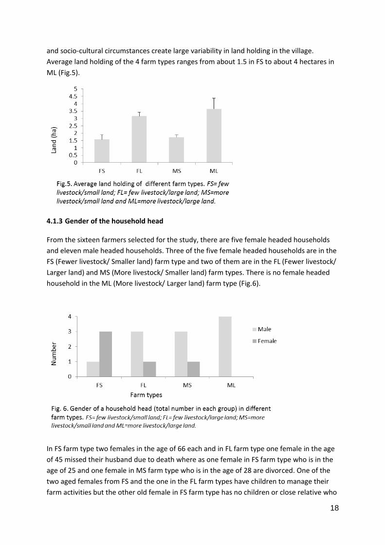
and socio-cultural circumstances create large variability in land holding in the village.
Average land holding of the 4 farm types ranges from about 1.5 in FS to about 4 hectares in
ML (Fig.5).
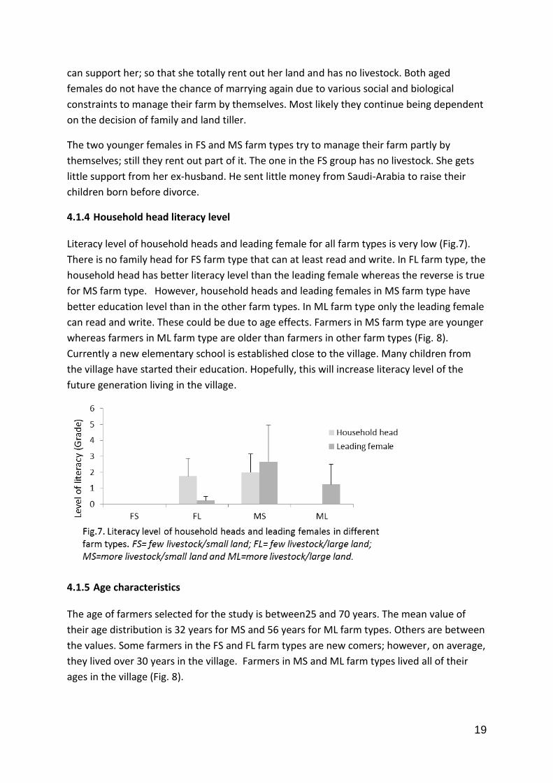
4.1.3 Gender of the household head
From the sixteen farmers selected for the study, there are five female headed households
and eleven male headed households. Three of the five female headed households are in the
FS (Fewer livestock/ Smaller land) farm type and two of them are in the FL (Fewer livestock/
Larger land) and MS (More livestock/ Smaller land) farm types. There is no female headed
household in the ML (More livestock/ Larger land) farm type (Fig.6).
In FS farm type two females in the age of 66 each and in FL farm type one female in the age
of 45 missed their husband due to death where as one female in FS farm type who is in the
age of 25 and one female in MS farm type who is in the age of 28 are divorced. One of the
two aged females from FS and the one in the FL farm types have children to manage their
farm activities but the other old female in FS farm type has no children or close relative who
19
can support her; so that she totally rent out her land and has no livestock. Both aged
females do not have the chance of marrying again due to various social and biological
constraints to manage their farm by themselves. Most likely they continue being dependent
on the decision of family and land tiller.
The two younger females in FS and MS farm types try to manage their farm partly by
themselves; still they rent out part of it. The one in the FS group has no livestock. She gets
little support from her ex-husband. He sent little money from Saudi-Arabia to raise their
children born before divorce.
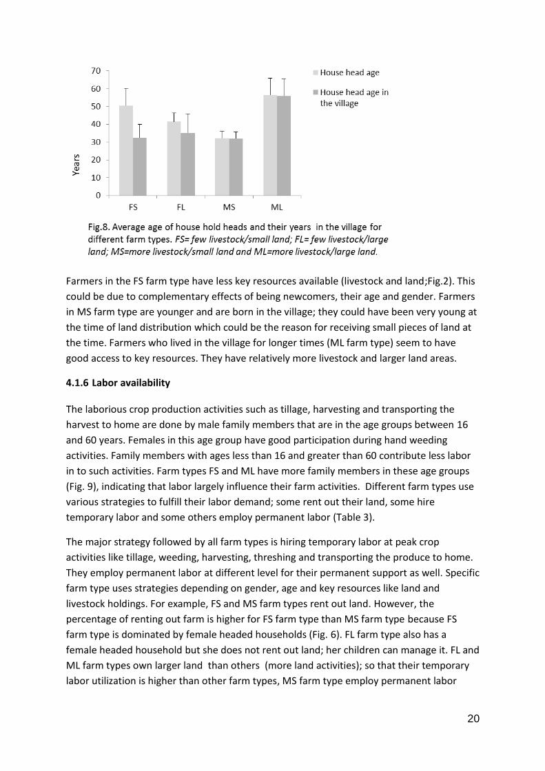
4.1.4 Household head literacy level
Literacy level of household heads and leading female for all farm types is very low (Fig.7).
There is no family head for FS farm type that can at least read and write. In FL farm type, the
household head has better literacy level than the leading female whereas the reverse is true
for MS farm type. However, household heads and leading females in MS farm type have
better education level than in the other farm types. In ML farm type only the leading female
can read and write. These could be due to age effects. Farmers in MS farm type are younger
whereas farmers in ML farm type are older than farmers in other farm types (Fig. 8).
Currently a new elementary school is established close to the village. Many children from
the village have started their education. Hopefully, this will increase literacy level of the
future generation living in the village.
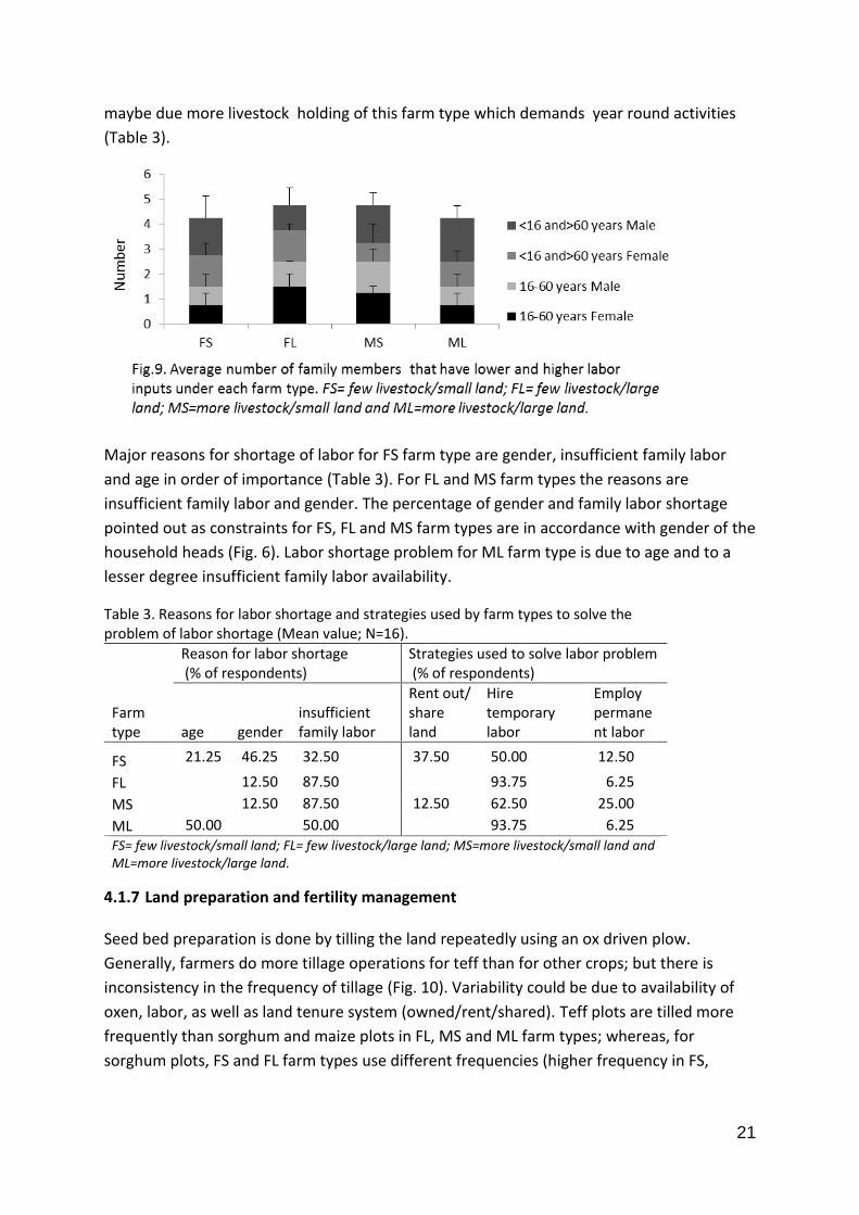
4.1.5 Age characteristics
The age of farmers selected for the study is between25 and 70 years. The mean value of
their age distribution is 32 years for MS and 56 years for ML farm types. Others are between
the values. Some farmers in the FS and FL farm types are new comers; however, on average,
they lived over 30 years in the village. Farmers in MS and ML farm types lived all of their
ages in the village (Fig. 8).
20
Farmers in the FS farm type have less key resources available (livestock and land;Fig.2). This
could be due to complementary effects of being newcomers, their age and gender. Farmers
in MS farm type are younger and are born in the village; they could have been very young at
the time of land distribution which could be the reason for receiving small pieces of land at
the time. Farmers who lived in the village for longer times (ML farm type) seem to have
good access to key resources. They have relatively more livestock and larger land areas.
4.1.6 Labor availability
The laborious crop production activities such as tillage, harvesting and transporting the
harvest to home are done by male family members that are in the age groups between 16
and 60 years. Females in this age group have good participation during hand weeding
activities. Family members with ages less than 16 and greater than 60 contribute less labor
in to such activities. Farm types FS and ML have more family members in these age groups
(Fig. 9), indicating that labor largely influence their farm activities. Different farm types use
various strategies to fulfill their labor demand; some rent out their land, some hire
temporary labor and some others employ permanent labor (Table 3).
The major strategy followed by all farm types is hiring temporary labor at peak crop
activities like tillage, weeding, harvesting, threshing and transporting the produce to home.
They employ permanent labor at different level for their permanent support as well. Specific
farm type uses strategies depending on gender, age and key resources like land and
livestock holdings. For example, FS and MS farm types rent out land. However, the
percentage of renting out farm is higher for FS farm type than MS farm type because FS
farm type is dominated by female headed households (Fig. 6). FL farm type also has a
female headed household but she does not rent out land; her children can manage it. FL and
ML farm types own larger land than others (more land activities); so that their temporary
labor utilization is higher than other farm types, MS farm type employ permanent labor
21
maybe due more livestock holding of this farm type which demands year round activities
(Table 3).
Major reasons for shortage of labor for FS farm type are gender, insufficient family labor
and age in order of importance (Table 3). For FL and MS farm types the reasons are
insufficient family labor and gender. The percentage of gender and family labor shortage
pointed out as constraints for FS, FL and MS farm types are in accordance with gender of the
household heads (Fig. 6). Labor shortage problem for ML farm type is due to age and to a
lesser degree insufficient family labor availability.
Table 3. Reasons for labor shortage and strategies used by farm types to solve the problem of labor shortage (Mean value; N=16).
Farm type
Reason for labor shortage (% of respondents)
Strategies used to solve labor problem (% of respondents)
age gender insufficient family labor
Rent out/ share land
Hire temporary labor
Employ permanent labor
FS 21.25 46.25 32.50 37.50 50.00 12.50
FL 12.50 87.50
93.75 6.25
MS 12.50 87.50 12.50 62.50 25.00
ML 50.00
50.00
93.75 6.25
FS= few livestock/small land; FL= few livestock/large land; MS=more livestock/small land and ML=more livestock/large land.
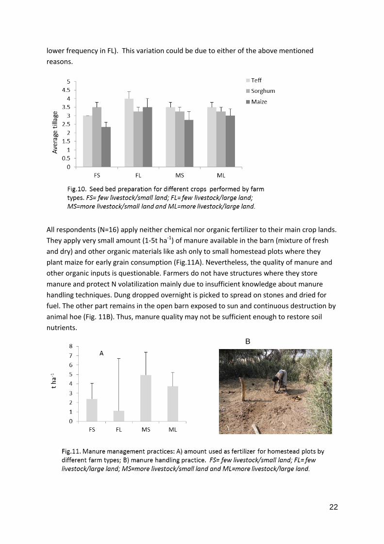
4.1.7 Land preparation and fertility management
Seed bed preparation is done by tilling the land repeatedly using an ox driven plow.
Generally, farmers do more tillage operations for teff than for other crops; but there is
inconsistency in the frequency of tillage (Fig. 10). Variability could be due to availability of
oxen, labor, as well as land tenure system (owned/rent/shared). Teff plots are tilled more
frequently than sorghum and maize plots in FL, MS and ML farm types; whereas, for
sorghum plots, FS and FL farm types use different frequencies (higher frequency in FS,
22
lower frequency in FL). This variation could be due to either of the above mentioned
reasons.
All respondents (N=16) apply neither chemical nor organic fertilizer to their main crop lands.
They apply very small amount (1-5t ha-1) of manure available in the barn (mixture of fresh
and dry) and other organic materials like ash only to small homestead plots where they
plant maize for early grain consumption (Fig.11A). Nevertheless, the quality of manure and
other organic inputs is questionable. Farmers do not have structures where they store
manure and protect N volatilization mainly due to insufficient knowledge about manure
handling techniques. Dung dropped overnight is picked to spread on stones and dried for
fuel. The other part remains in the open barn exposed to sun and continuous destruction by
animal hoe (Fig. 11B). Thus, manure quality may not be sufficient enough to restore soil
nutrients.
B
23
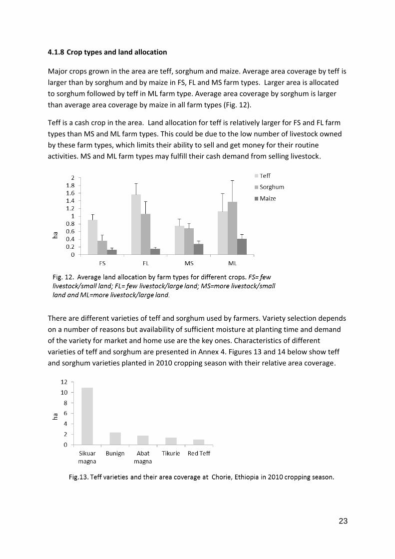
4.1.8 Crop types and land allocation
Major crops grown in the area are teff, sorghum and maize. Average area coverage by teff is
larger than by sorghum and by maize in FS, FL and MS farm types. Larger area is allocated
to sorghum followed by teff in ML farm type. Average area coverage by sorghum is larger
than average area coverage by maize in all farm types (Fig. 12).
Teff is a cash crop in the area. Land allocation for teff is relatively larger for FS and FL farm
types than MS and ML farm types. This could be due to the low number of livestock owned
by these farm types, which limits their ability to sell and get money for their routine
activities. MS and ML farm types may fulfill their cash demand from selling livestock.
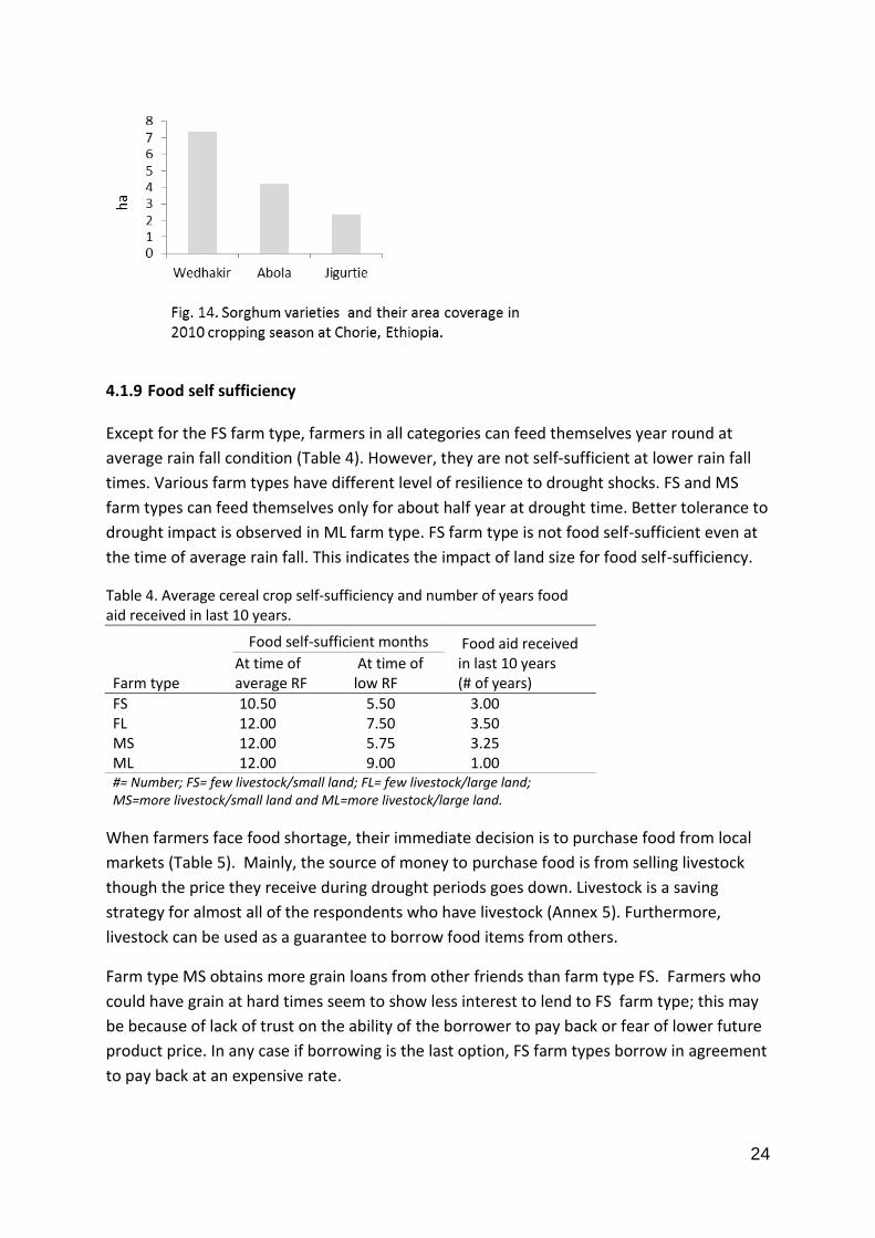
There are different varieties of teff and sorghum used by farmers. Variety selection depends
on a number of reasons but availability of sufficient moisture at planting time and demand
of the variety for market and home use are the key ones. Characteristics of different
varieties of teff and sorghum are presented in Annex 4. Figures 13 and 14 below show teff
and sorghum varieties planted in 2010 cropping season with their relative area coverage.
24
4.1.9 Food self sufficiency
Except for the FS farm type, farmers in all categories can feed themselves year round at
average rain fall condition (Table 4). However, they are not self-sufficient at lower rain fall
times. Various farm types have different level of resilience to drought shocks. FS and MS
farm types can feed themselves only for about half year at drought time. Better tolerance to
drought impact is observed in ML farm type. FS farm type is not food self-sufficient even at
the time of average rain fall. This indicates the impact of land size for food self-sufficiency.
Table 4. Average cereal crop self-sufficiency and number of years food aid received in last 10 years.
Farm type
Food self-sufficient months Food aid received in last 10 years (# of years)
At time of average RF
At time of low RF
FS 10.50 5.50 3.00 FL 12.00 7.50 3.50 MS 12.00 5.75 3.25 ML 12.00 9.00 1.00 #= Number; FS= few livestock/small land; FL= few livestock/large land; MS=more livestock/small land and ML=more livestock/large land.
When farmers face food shortage, their immediate decision is to purchase food from local
markets (Table 5). Mainly, the source of money to purchase food is from selling livestock
though the price they receive during drought periods goes down. Livestock is a saving
strategy for almost all of the respondents who have livestock (Annex 5). Furthermore,
livestock can be used as a guarantee to borrow food items from others.
Farm type MS obtains more grain loans from other friends than farm type FS. Farmers who
could have grain at hard times seem to show less interest to lend to FS farm type; this may
be because of lack of trust on the ability of the borrower to pay back or fear of lower future
product price. In any case if borrowing is the last option, FS farm types borrow in agreement
to pay back at an expensive rate.
25
Table 5. Percentage of food remedial sources at scarcity periods.
Farm types Purchase Subsidy Given by others Borrow *
FS 75.00 12.50 12.50
FL 71.25 8.75 20.00
MS 50.00 50.00
ML 100.00 FS= few livestock/small land; FL= few livestock/large land; MS=more livestock/small land and ML=more livestock/large land. * Borrow at expensive return: If they borrow 1 quintal of sorghum, the agreement could be to
pay back 1 quintal of teff or 1.5- 2 quintals of sorghum at the next harvesting season.
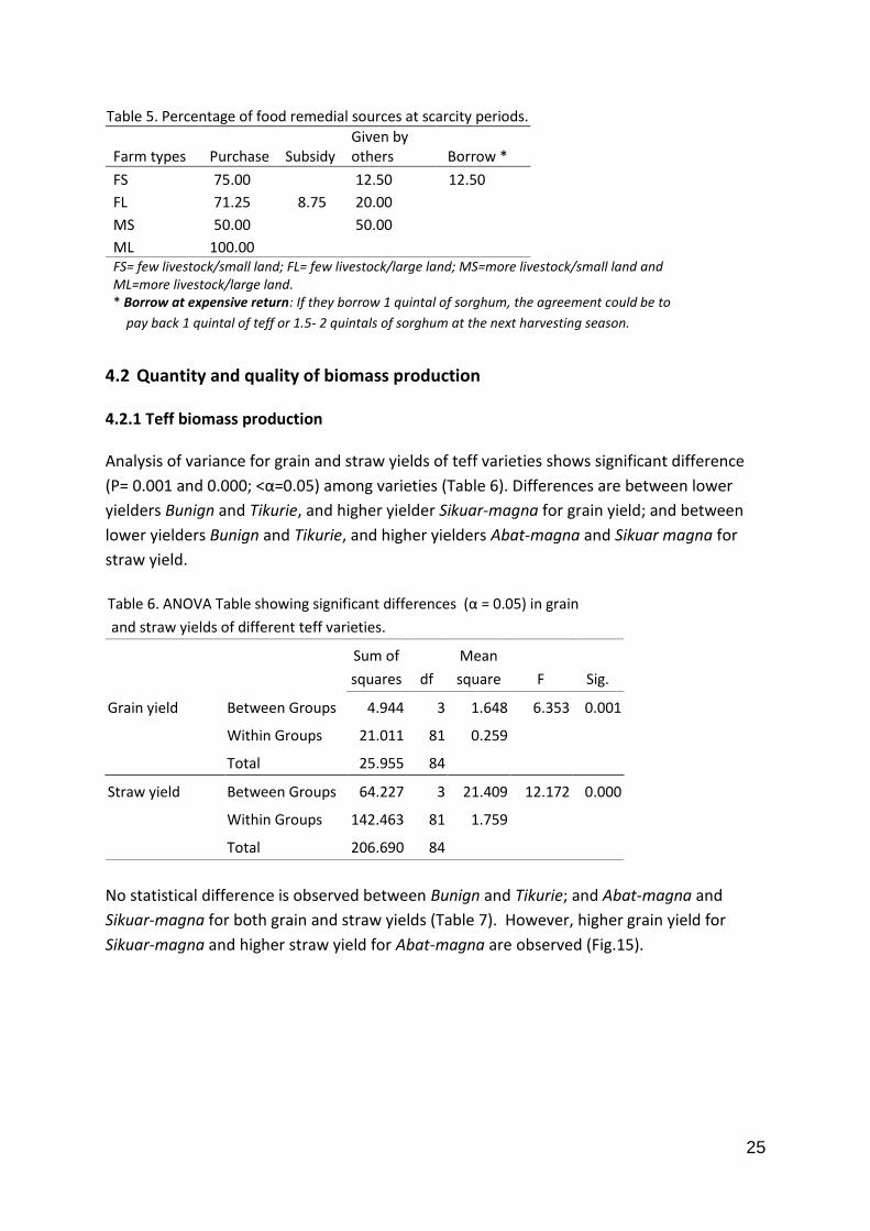
4.2 Quantity and quality of biomass production
4.2.1 Teff biomass production
Analysis of variance for grain and straw yields of teff varieties shows significant difference
(P= 0.001 and 0.000; <α=0.05) among varieties (Table 6). Differences are between lower
yielders Bunign and Tikurie, and higher yielder Sikuar-magna for grain yield; and between
lower yielders Bunign and Tikurie, and higher yielders Abat-magna and Sikuar magna for
straw yield.
Table 6. ANOVA Table showing significant differences (α = 0.05) in grain
and straw yields of different teff varieties.
Sum of
squares df
Mean
square F Sig.
Grain yield Between Groups 4.944 3 1.648 6.353 0.001
Within Groups 21.011 81 0.259
Total 25.955 84
Straw yield Between Groups 64.227 3 21.409 12.172 0.000
Within Groups 142.463 81 1.759
Total 206.690 84
No statistical difference is observed between Bunign and Tikurie; and Abat-magna and
Sikuar-magna for both grain and straw yields (Table 7). However, higher grain yield for
Sikuar-magna and higher straw yield for Abat-magna are observed (Fig.15).
26
Table 7. Mean separation for grain and straw yields of teff varieties.
Local names of teff
varieties
Grain yield
(t ha-1)
Straw yield
(t ha-1)
Dunkcan1 Buningn 0.8344a 2.1160c
Tikurie 1.0656a 3.2200c
Abat-magna 1.2158a 1.2158ab 5.5122d
Sikuar-magna 1.600b 5.1753d
Sig. 0.089 0.6010
Farmers were asked to estimate grain and straw yields. Analysis indicates very low
correlation between measured and farmers’ estimation(both grain and straw yield;
r2=0.031; r2=0.0654 respectively; Fig. 16).
For straw yield, higher difference is observed between measured and farmers’ estimation in
FS farm type (Fig.17). This could be due to the influence of gender. In this farm group the
ratio of female to male is 3: 1 (Fig.4); female head households either share/rent out their
land or give all land management activities to their family (son/daughter if applicable; Annex
6); so that they have less control on land activities which hinders them to adequately
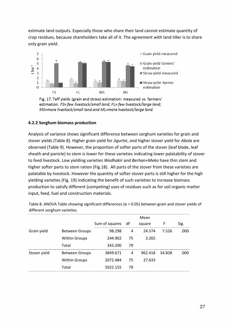
27
estimate land outputs. Especially those who share their land cannot estimate quantity of
crop residues, because shareholders take all of it. The agreement with land tiller is to share
only grain yield.
4.2.2 Sorghum biomass production
Analysis of variance shows significant difference between sorghum varieties for grain and
stover yields (Table 8). Higher grain yield for Jigurtie, and higher stover yield for Abola are
observed (Table 9). However, the proportion of softer parts of the stover (leaf blade, leaf
sheath and panicle) to stem is lower for these varieties indicating lower palatability of stover
to feed livestock. Low yielding varieties Wedhakir and Berhan+Meko have thin stem and
higher softer parts to stem ration (Fig.18). All parts of the stover from these varieties are
palatable by livestock. However the quantity of softer stover parts is still higher for the high
yielding varieties (Fig. 19) indicating the benefit of such varieties to increase biomass
production to satisfy different (competing) uses of residues such as for soil organic matter
input, feed, fuel and construction materials.
Table 8. ANOVA Table showing significant differences (α = 0.05) between grain and stover yields of
different sorghum varieties.
Sum of squares df
Mean
square F Sig.
Grain yield Between Groups 98.298 4 24.574 7.526 .000
Within Groups 244.902 75 3.265
Total 343.200 79
Stover yield Between Groups 3849.671 4 962.418 34.828 .000
Within Groups 2072.484 75 27.633
Total 5922.155 79
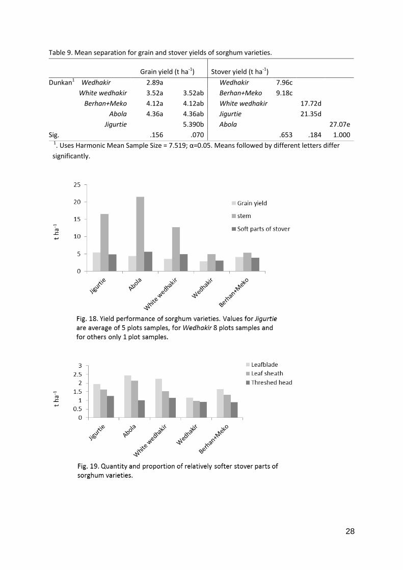
28
Table 9. Mean separation for grain and stover yields of sorghum varieties.
Grain yield (t ha-1) Stover yield (t ha-1)
Dunkan1 Wedhakir 2.89a Wedhakir 7.96c
White wedhakir 3.52a 3.52ab Berhan+Meko 9.18c
Berhan+Meko 4.12a 4.12ab White wedhakir 17.72d
Abola 4.36a 4.36ab Jigurtie 21.35d
Jigurtie 5.390b Abola 27.07e
Sig. .156 .070 .653 .184 1.000 1. Uses Harmonic Mean Sample Size = 7.519; α=0.05. Means followed by different letters differ
significantly.
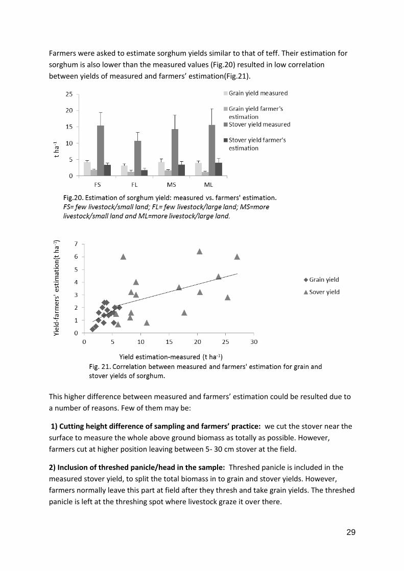
29
Farmers were asked to estimate sorghum yields similar to that of teff. Their estimation for
sorghum is also lower than the measured values (Fig.20) resulted in low correlation
between yields of measured and farmers’ estimation(Fig.21).
This higher difference between measured and farmers’ estimation could be resulted due to
a number of reasons. Few of them may be:
1) Cutting height difference of sampling and farmers’ practice: we cut the stover near the
surface to measure the whole above ground biomass as totally as possible. However,
farmers cut at higher position leaving between 5- 30 cm stover at the field.
2) Inclusion of threshed panicle/head in the sample: Threshed panicle is included in the
measured stover yield, to split the total biomass in to grain and stover yields. However,
farmers normally leave this part at field after they thresh and take grain yields. The threshed
panicle is left at the threshing spot where livestock graze it over there.
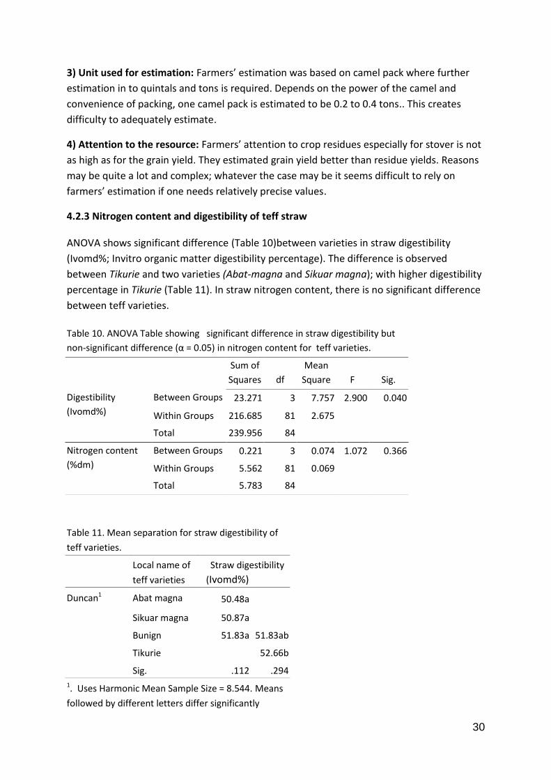
30
3) Unit used for estimation: Farmers’ estimation was based on camel pack where further
estimation in to quintals and tons is required. Depends on the power of the camel and
convenience of packing, one camel pack is estimated to be 0.2 to 0.4 tons.. This creates
difficulty to adequately estimate.
4) Attention to the resource: Farmers’ attention to crop residues especially for stover is not
as high as for the grain yield. They estimated grain yield better than residue yields. Reasons
may be quite a lot and complex; whatever the case may be it seems difficult to rely on
farmers’ estimation if one needs relatively precise values.
4.2.3 Nitrogen content and digestibility of teff straw
ANOVA shows significant difference (Table 10)between varieties in straw digestibility
(Ivomd%; Invitro organic matter digestibility percentage). The difference is observed
between Tikurie and two varieties (Abat-magna and Sikuar magna); with higher digestibility
percentage in Tikurie (Table 11). In straw nitrogen content, there is no significant difference
between teff varieties.
Table 10. ANOVA Table showing significant difference in straw digestibility but
non-significant difference (α = 0.05) in nitrogen content for teff varieties.
Sum of
Squares df
Mean
Square F Sig.
Digestibility
(Ivomd%)
Between Groups 23.271 3 7.757 2.900 0.040
Within Groups 216.685 81 2.675
Total 239.956 84
Nitrogen content
(%dm)
Between Groups 0.221 3 0.074 1.072 0.366
Within Groups 5.562 81 0.069
Total 5.783 84
Table 11. Mean separation for straw digestibility of
teff varieties.
Local name of
teff varieties
Straw digestibility
(Ivomd%)
Duncan1 Abat magna 50.48a
Sikuar magna 50.87a
Bunign 51.83a 51.83ab
Tikurie 52.66b
Sig. .112 .294
1. Uses Harmonic Mean Sample Size = 8.544. Means
followed by different letters differ significantly
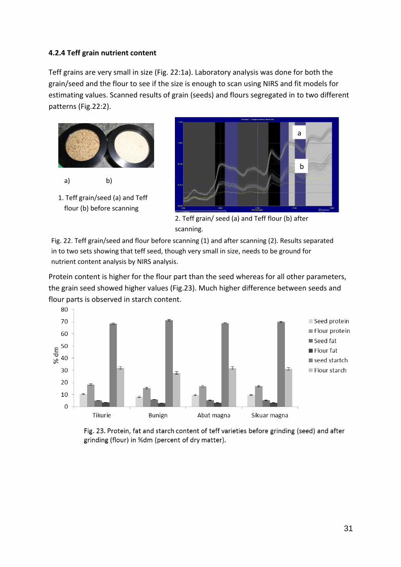
31
4.2.4 Teff grain nutrient content
Teff grains are very small in size (Fig. 22:1a). Laboratory analysis was done for both the
grain/seed and the flour to see if the size is enough to scan using NIRS and fit models for
estimating values. Scanned results of grain (seeds) and flours segregated in to two different
patterns (Fig.22:2).
Protein content is higher for the flour part than the seed whereas for all other parameters,
the grain seed showed higher values (Fig.23). Much higher difference between seeds and
flour parts is observed in starch content.
Fig. 22. Teff grain/seed and flour before scanning (1) and after scanning (2). Results separated
in to two sets showing that teff seed, though very small in size, needs to be ground for
nutrient content analysis by NIRS analysis.
2. Teff grain/ seed (a) and Teff flour (b) after
scanning.
a) b)
1. Teff grain/seed (a) and Teff
flour (b) before scanning
a
b
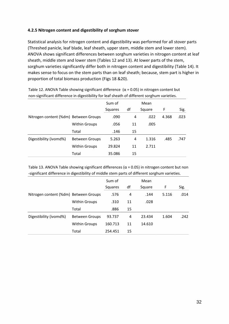
32
4.2.5 Nitrogen content and digestibility of sorghum stover
Statistical analysis for nitrogen content and digestibility was performed for all stover parts
(Threshed panicle, leaf blade, leaf sheath, upper stem, middle stem and lower stem).
ANOVA shows significant differences between sorghum varieties in nitrogen content at leaf
sheath, middle stem and lower stem (Tables 12 and 13). At lower parts of the stem,
sorghum varieties significantly differ both in nitrogen content and digestibility (Table 14). It
makes sense to focus on the stem parts than on leaf sheath; because, stem part is higher in
proportion of total biomass production (Figs 18 &20).
Table 12. ANOVA Table showing significant difference (α = 0.05) in nitrogen content but
non-significant difference in digestibility for leaf sheath of different sorghum varieties.
Sum of
Squares df
Mean
Square F Sig.
Nitrogen content (%dm) Between Groups .090 4 .022 4.368 .023
Within Groups .056 11 .005
Total .146 15
Digestibility (ivomd%) Between Groups 5.263 4 1.316 .485 .747
Within Groups 29.824 11 2.711
Total 35.086 15
Table 13. ANOVA Table showing significant differences (α = 0.05) in nitrogen content but non
-significant difference in digestibility of middle stem parts of different sorghum varieties.
Sum of
Squares df
Mean
Square F Sig.
Nitrogen content (%dm) Between Groups .576 4 .144 5.116 .014
Within Groups .310 11 .028
Total .886 15
Digestibility (ivomd%) Between Groups 93.737 4 23.434 1.604 .242
Within Groups 160.713 11 14.610
Total 254.451 15
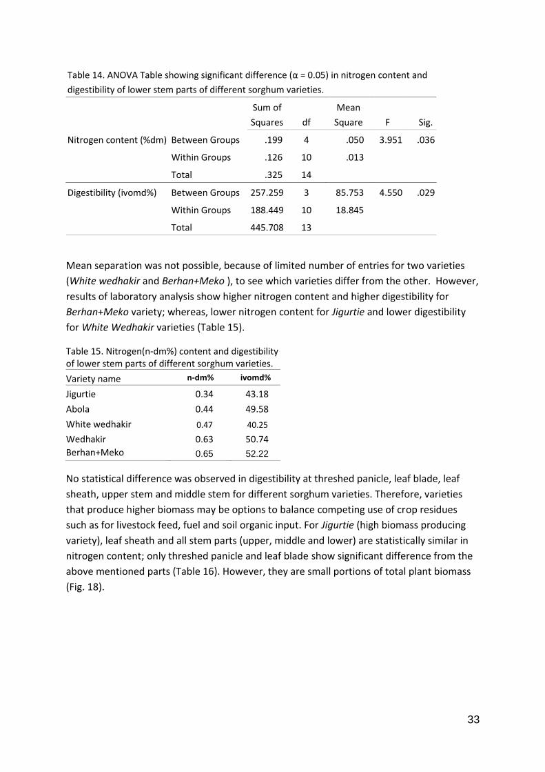
33
Table 14. ANOVA Table showing significant difference (α = 0.05) in nitrogen content and
digestibility of lower stem parts of different sorghum varieties.
Sum of
Squares df
Mean
Square F Sig.
Nitrogen content (%dm) Between Groups .199 4 .050 3.951 .036
Within Groups .126 10 .013
Total .325 14
Digestibility (ivomd%) Between Groups 257.259 3 85.753 4.550 .029
Within Groups 188.449 10 18.845
Total 445.708 13
Mean separation was not possible, because of limited number of entries for two varieties
(White wedhakir and Berhan+Meko ), to see which varieties differ from the other. However,
results of laboratory analysis show higher nitrogen content and higher digestibility for
Berhan+Meko variety; whereas, lower nitrogen content for Jigurtie and lower digestibility
for White Wedhakir varieties (Table 15).
Table 15. Nitrogen(n-dm%) content and digestibility of lower stem parts of different sorghum varieties.
Variety name n-dm% ivomd%
Jigurtie 0.34 43.18
Abola 0.44 49.58
White wedhakir 0.47 40.25
Wedhakir 0.63 50.74
Berhan+Meko 0.65 52.22
No statistical difference was observed in digestibility at threshed panicle, leaf blade, leaf
sheath, upper stem and middle stem for different sorghum varieties. Therefore, varieties
that produce higher biomass may be options to balance competing use of crop residues
such as for livestock feed, fuel and soil organic input. For Jigurtie (high biomass producing
variety), leaf sheath and all stem parts (upper, middle and lower) are statistically similar in
nitrogen content; only threshed panicle and leaf blade show significant difference from the
above mentioned parts (Table 16). However, they are small portions of total plant biomass
(Fig. 18).
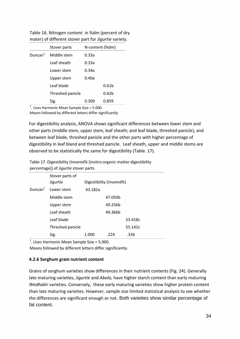
34
Table 16. Nitrogen content in %dm (percent of dry
mater) of different stover part for Jigurtie variety.
Stover parts N-content (%dm)
Duncan1 Middle stem 0.33a
Leaf sheath 0.33a
Lower stem 0.34a
Upper stem 0.40a
Leaf blade 0.61b
Threshed panicle 0.62b
Sig. 0.309 0.859 1. Uses Harmonic Mean Sample Size = 5.000.
Means followed by different letters differ significantly
For digestibility analysis, ANOVA shows significant differences between lower stem and
other parts (middle stem, upper stem, leaf sheath; and leaf blade, threshed panicle), and
between leaf blade, threshed panicle and the other parts with higher percentage of
digestibility in leaf bland and threshed panicle. Leaf sheath, upper and middle stems are
observed to be statistically the same for digestibility (Table. 17).
Table 17. Digestibility (Invomd% [invitro organic matter digestibility
percentage]) of Jigurtie stover parts.
Stover parts of
Jigurtie Digestibility (Invomd%)
Duncan1 Lower stem 43.182a
Middle stem 47.050b
Upper stem 49.256b
Leaf sheath 49.366b
Leaf blade 53.418c
Threshed panicle 55.142c
Sig. 1.000 .224 .336 1. Uses Harmonic Mean Sample Size = 5.000.
Means followed by different letters differ significantly.
4.2.6 Sorghum grain nutrient content
Grains of sorghum varieties show differences in their nutrient contents (Fig. 24). Generally
late maturing varieties, Jigurtie and Abola, have higher starch content than early maturing
Wedhakir varieties. Conversely, these early maturing varieties show higher protein content
than late maturing varieties. However, sample size limited statistical analysis to see whether
the differences are significant enough or not. Both varieties show similar percentage of
fat content.
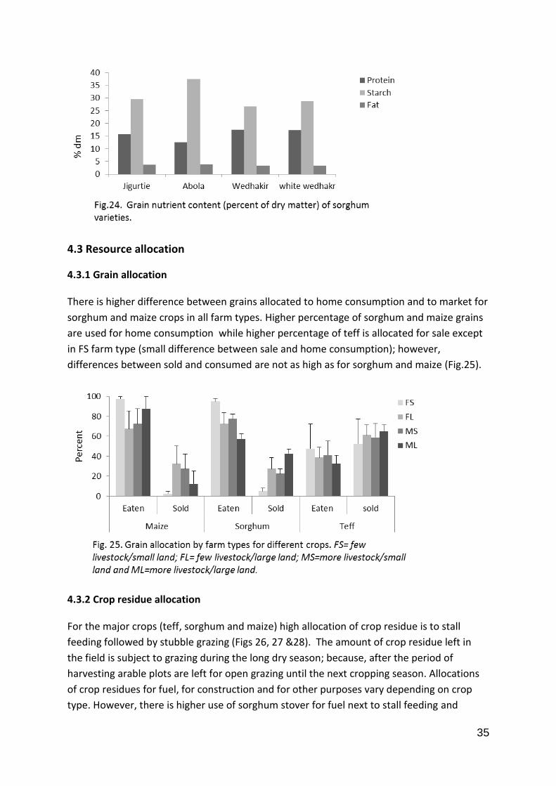
35
4.3 Resource allocation
4.3.1 Grain allocation
There is higher difference between grains allocated to home consumption and to market for
sorghum and maize crops in all farm types. Higher percentage of sorghum and maize grains
are used for home consumption while higher percentage of teff is allocated for sale except
in FS farm type (small difference between sale and home consumption); however,
differences between sold and consumed are not as high as for sorghum and maize (Fig.25).
4.3.2 Crop residue allocation
For the major crops (teff, sorghum and maize) high allocation of crop residue is to stall
feeding followed by stubble grazing (Figs 26, 27 &28). The amount of crop residue left in
the field is subject to grazing during the long dry season; because, after the period of
harvesting arable plots are left for open grazing until the next cropping season. Allocations
of crop residues for fuel, for construction and for other purposes vary depending on crop
type. However, there is higher use of sorghum stover for fuel next to stall feeding and
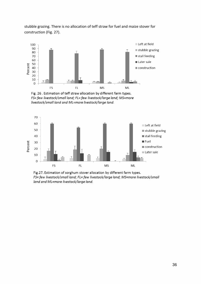
36
stubble grazing. There is no allocation of teff straw for fuel and maize stover for
construction (Fig. 27).
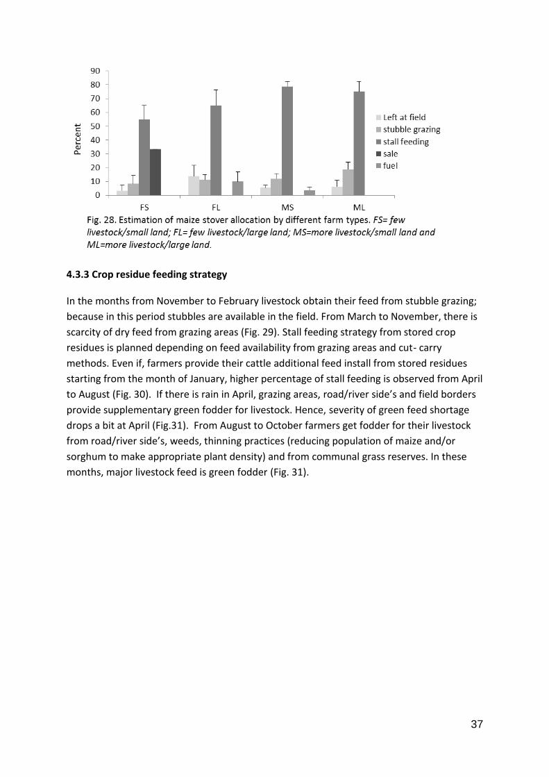
37
4.3.3 Crop residue feeding strategy
In the months from November to February livestock obtain their feed from stubble grazing;
because in this period stubbles are available in the field. From March to November, there is
scarcity of dry feed from grazing areas (Fig. 29). Stall feeding strategy from stored crop
residues is planned depending on feed availability from grazing areas and cut- carry
methods. Even if, farmers provide their cattle additional feed install from stored residues
starting from the month of January, higher percentage of stall feeding is observed from April
to August (Fig. 30). If there is rain in April, grazing areas, road/river side’s and field borders
provide supplementary green fodder for livestock. Hence, severity of green feed shortage
drops a bit at April (Fig.31). From August to October farmers get fodder for their livestock
from road/river side’s, weeds, thinning practices (reducing population of maize and/or
sorghum to make appropriate plant density) and from communal grass reserves. In these
months, major livestock feed is green fodder (Fig. 31).
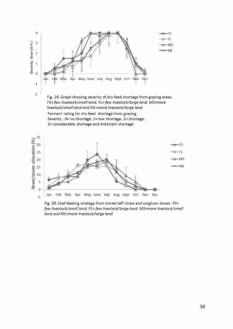
38
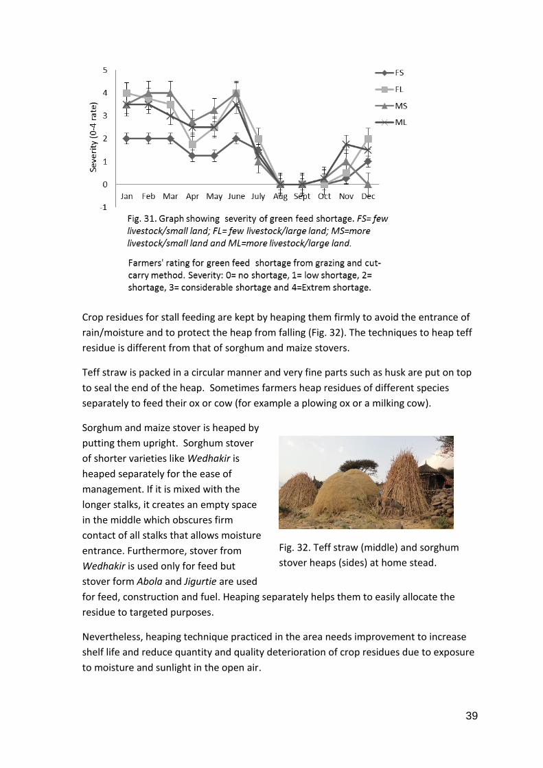
39
Fig. 32. Teff straw (middle) and sorghum
stover heaps (sides) at home stead.
Crop residues for stall feeding are kept by heaping them firmly to avoid the entrance of
rain/moisture and to protect the heap from falling (Fig. 32). The techniques to heap teff
residue is different from that of sorghum and maize stovers.
Teff straw is packed in a circular manner and very fine parts such as husk are put on top
to seal the end of the heap. Sometimes farmers heap residues of different species
separately to feed their ox or cow (for example a plowing ox or a milking cow).
Sorghum and maize stover is heaped by
putting them upright. Sorghum stover
of shorter varieties like Wedhakir is
heaped separately for the ease of
management. If it is mixed with the
longer stalks, it creates an empty space
in the middle which obscures firm
contact of all stalks that allows moisture
entrance. Furthermore, stover from
Wedhakir is used only for feed but
stover form Abola and Jigurtie are used
for feed, construction and fuel. Heaping separately helps them to easily allocate the
residue to targeted purposes.
Nevertheless, heaping technique practiced in the area needs improvement to increase
shelf life and reduce quantity and quality deterioration of crop residues due to exposure
to moisture and sunlight in the open air.
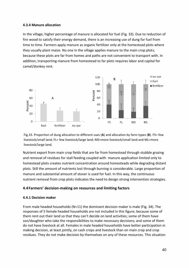
40
4.3.4 Manure allocation
In the village, higher percentage of manure is allocated for fuel (Fig. 33). Due to reduction of
fire wood to satisfy their energy demand, there is an increasing use of dung for fuel from
time to time. Farmers apply manure as organic fertilizer only at the homestead plots where
they usually plant maize. No one in the village applies manure to the main crop plots;
because these plots are far from homes and paths are not convenient to transport with. In
addition, transporting manure from homestead to far plots requires labor and capital for
camel/donkey rent.
Nutrient export from main crop fields that are far from homestead through stubble grazing
and removal of residues for stall feeding coupled with manure application limited only to
homestead plots creates nutrient concentration around homesteads while degrading distant
plots. Still the amount of nutrients lost through burning is considerable. Large proportion of
manure and substantial amount of stover is used for fuel. In this way, the continuous
nutrient removal from crop plots indicates the need to design strong intervention strategies.
4.4 Farmers’ decision-making on resources and limiting factors
4.4.1 Decision maker
From male headed households (N=11) the dominant decision maker is male (Fig. 34). The responses of 5 female headed households are not included in this figure; because some of them rent out their land so that they can’t decide on land activities; some of them have son/daughter who take the responsibilities to make necessary decisions; and some of them do not have livestock at all. Females in male headed households have better participation in making decision, at least jointly, on cash crops and livestock than on main crop and crop residues. They do not make decision by themselves on any of these resources. This situation
Fig.33. Proportion of dung allocation to different uses (A) and allocation by farm types (B). FS= few
livestock/small land; FL= few livestock/large land; MS=more livestock/small land and ML=more
livestock/large land.
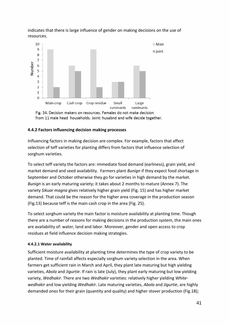
41
indicates that there is large influence of gender on making decisions on the use of resources.
4.4.2 Factors influencing decision making processes
Influencing factors in making decision are complex. For example, factors that affect
selection of teff varieties for planting differs from factors that influence selection of
sorghum varieties.
To select teff variety the factors are: immediate food demand (earliness), grain yield, and
market demand and seed availability. Farmers plant Bunign if they expect food shortage in
September and October otherwise they go for varieties in high demand by the market.
Bunign is an early maturing variety; it takes about 2 months to mature (Annex 7). The
variety Sikuar magna gives relatively higher grain yield (Fig. 15) and has higher market
demand. That could be the reason for the higher area coverage in the production season
(Fig.13) because teff is the main cash crop in the area (Fig. 25).
To select sorghum variety the main factor is moisture availability at planting time. Though
there are a number of reasons for making decisions in the production system, the main ones
are availability of: water, land and labor. Moreover, gender and open access to crop
residues at field influence decision making strategies.
4.4.2.1 Water availability
Sufficient moisture availability at planting time determines the type of crop variety to be
planted. Time of rainfall affects especially sorghum variety selection in the area. When
farmers get sufficient rain in March and April, they plant late maturing but high yielding
varieties, Abola and Jigurtie. If rain is late (July), they plant early maturing but low yielding
variety, Wedhakir. There are two Wedhakir varieties: relatively higher yielding White-
wedhakir and low yielding Wedhakir. Late maturing varieties, Abola and Jigurtie, are highly
demanded ones for their grain (quantity and quality) and higher stover production (Fig.18);
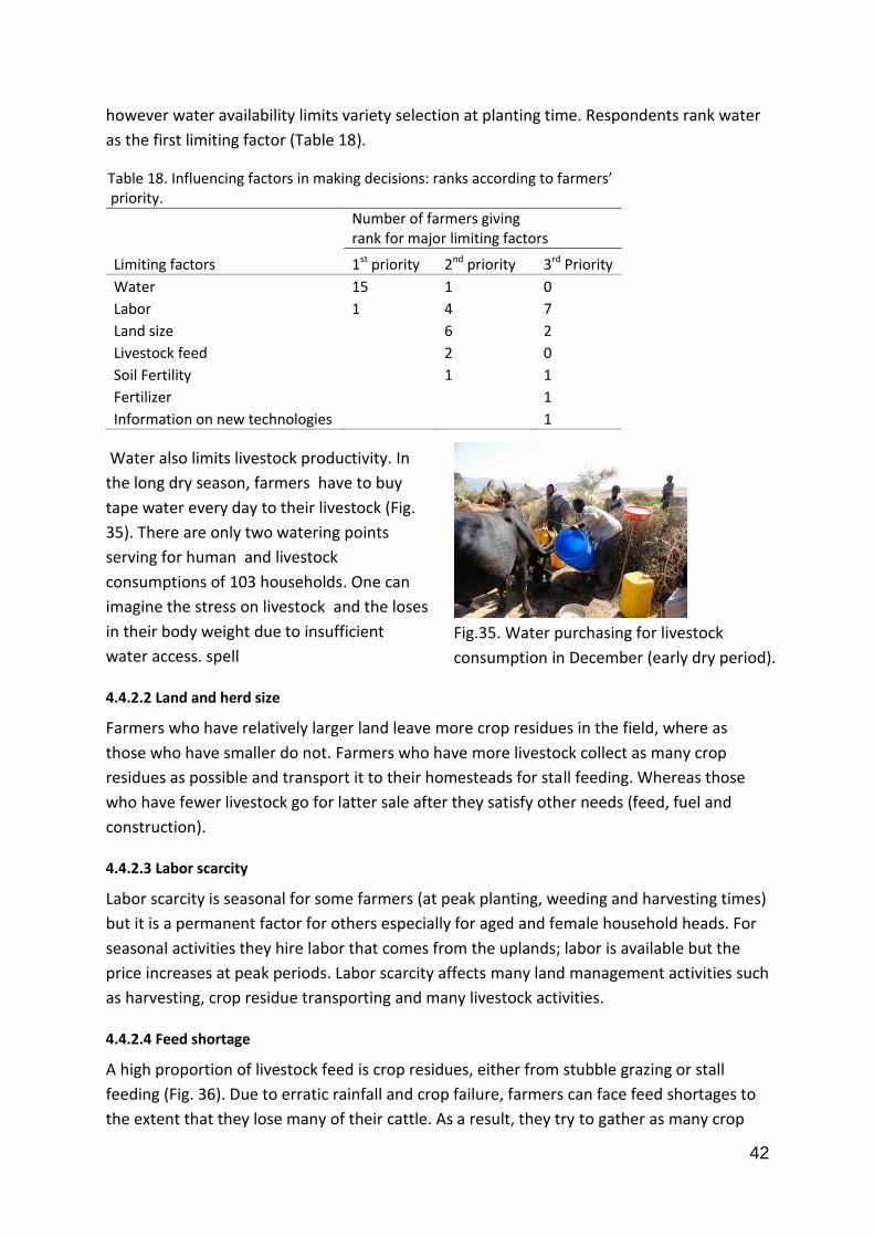
42
Fig.35. Water purchasing for livestock
consumption in December (early dry period).
however water availability limits variety selection at planting time. Respondents rank water
as the first limiting factor (Table 18).
Table 18. Influencing factors in making decisions: ranks according to farmers’ priority.
Limiting factors
Number of farmers giving rank for major limiting factors
1st priority 2nd priority 3rd Priority
Water 15 1 0
Labor 1 4 7
Land size 6 2
Livestock feed 2 0
Soil Fertility 1 1
Fertilizer 1
Information on new technologies 1
Water also limits livestock productivity. In
the long dry season, farmers have to buy
tape water every day to their livestock (Fig.
35). There are only two watering points
serving for human and livestock
consumptions of 103 households. One can
imagine the stress on livestock and the loses
in their body weight due to insufficient
water access. spell
4.4.2.2 Land and herd size
Farmers who have relatively larger land leave more crop residues in the field, where as
those who have smaller do not. Farmers who have more livestock collect as many crop
residues as possible and transport it to their homesteads for stall feeding. Whereas those
who have fewer livestock go for latter sale after they satisfy other needs (feed, fuel and
construction).
4.4.2.3 Labor scarcity
Labor scarcity is seasonal for some farmers (at peak planting, weeding and harvesting times)
but it is a permanent factor for others especially for aged and female household heads. For
seasonal activities they hire labor that comes from the uplands; labor is available but the
price increases at peak periods. Labor scarcity affects many land management activities such
as harvesting, crop residue transporting and many livestock activities.
4.4.2.4 Feed shortage
A high proportion of livestock feed is crop residues, either from stubble grazing or stall
feeding (Fig. 36). Due to erratic rainfall and crop failure, farmers can face feed shortages to
the extent that they lose many of their cattle. As a result, they try to gather as many crop
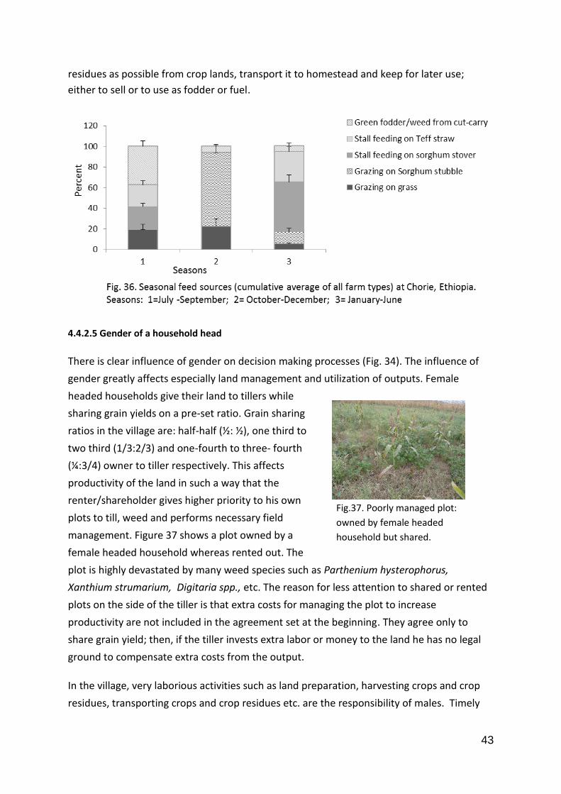
43
Fig.37. Poorly managed plot:
owned by female headed
household but shared.
residues as possible from crop lands, transport it to homestead and keep for later use;
either to sell or to use as fodder or fuel.
4.4.2.5 Gender of a household head
There is clear influence of gender on decision making processes (Fig. 34). The influence of
gender greatly affects especially land management and utilization of outputs. Female
headed households give their land to tillers while
sharing grain yields on a pre-set ratio. Grain sharing
ratios in the village are: half-half (½: ½), one third to
two third (1/3:2/3) and one-fourth to three- fourth
(¼:3/4) owner to tiller respectively. This affects
productivity of the land in such a way that the
renter/shareholder gives higher priority to his own
plots to till, weed and performs necessary field
management. Figure 37 shows a plot owned by a
female headed household whereas rented out. The
plot is highly devastated by many weed species such as Parthenium hysterophorus,
Xanthium strumarium, Digitaria spp., etc. The reason for less attention to shared or rented
plots on the side of the tiller is that extra costs for managing the plot to increase
productivity are not included in the agreement set at the beginning. They agree only to
share grain yield; then, if the tiller invests extra labor or money to the land he has no legal
ground to compensate extra costs from the output.
In the village, very laborious activities such as land preparation, harvesting crops and crop
residues, transporting crops and crop residues etc. are the responsibility of males. Timely
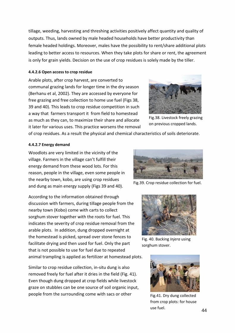
44
Fig. 40. Backing Injera using
sorghum stover.
Fig.41. Dry dung collected
from crop plots: for house
use fuel.
Fig.38. Livestock freely grazing
on previous cropped lands.
Fig.39. Crop residue collection for fuel.
tillage, weeding, harvesting and threshing activities positively affect quantity and quality of
outputs. Thus, lands owned by male headed households have better productivity than
female headed holdings. Moreover, males have the possibility to rent/share additional plots
leading to better access to resources. When they take plots for share or rent, the agreement
is only for grain yields. Decision on the use of crop residues is solely made by the tiller.
4.4.2.6 Open access to crop residue
Arable plots, after crop harvest, are converted to
communal grazing lands for longer time in the dry season
(Berhanu et al, 2002). They are accessed by everyone for
free grazing and free collection to home use fuel (Figs 38,
39 and 40). This leads to crop residue competition in such
a way that farmers transport it from field to homestead
as much as they can, to maximize their share and allocate
it later for various uses. This practice worsens the removal
of crop residues. As a result the physical and chemical characteristics of soils deteriorate.
4.4.2.7 Energy demand
Woodlots are very limited in the vicinity of the
village. Farmers in the village can’t fulfill their
energy demand from these wood lots. For this
reason, people in the village, even some people in
the nearby town, kobo, are using crop residues
and dung as main energy supply (Figs 39 and 40).
According to the information obtained through
discussion with farmers, during tillage people from the
nearby town (Kobo) come with carts to collect
sorghum stover together with the roots for fuel. This
indicates the severity of crop residue removal from the
arable plots. In addition, dung dropped overnight at
the homestead is picked, spread over stone fences to
facilitate drying and then used for fuel. Only the part
that is not possible to use for fuel due to repeated
animal trampling is applied as fertilizer at homestead plots.
Similar to crop residue collection, in-situ dung is also
removed freely for fuel after it dries in the field (Fig. 41).
Even though dung dropped at crop fields while livestock
graze on stubbles can be one source of soil organic input,
people from the surrounding come with sacs or other
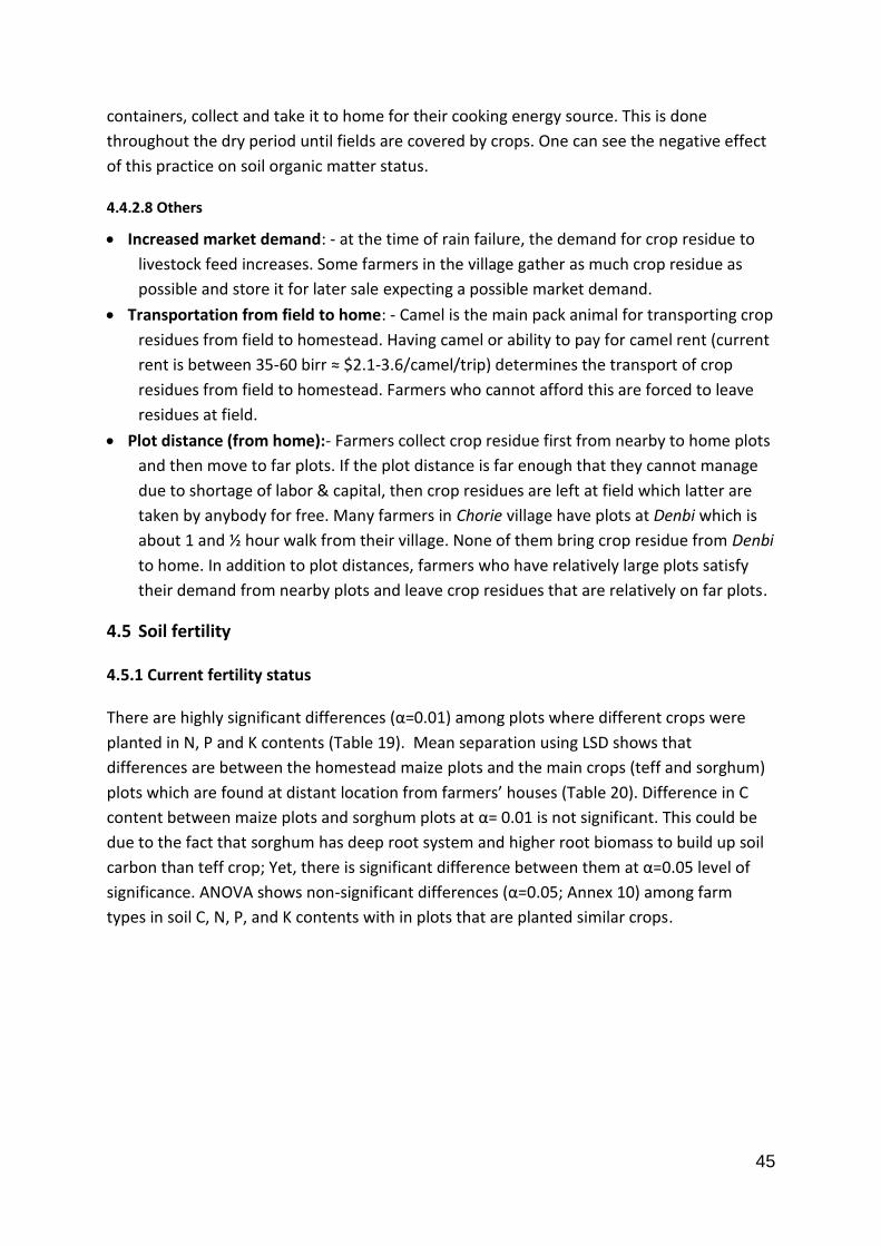
45
containers, collect and take it to home for their cooking energy source. This is done
throughout the dry period until fields are covered by crops. One can see the negative effect
of this practice on soil organic matter status.
4.4.2.8 Others
Increased market demand: - at the time of rain failure, the demand for crop residue to
livestock feed increases. Some farmers in the village gather as much crop residue as
possible and store it for later sale expecting a possible market demand.
Transportation from field to home: - Camel is the main pack animal for transporting crop
residues from field to homestead. Having camel or ability to pay for camel rent (current
rent is between 35-60 birr ≈ $2.1-3.6/camel/trip) determines the transport of crop
residues from field to homestead. Farmers who cannot afford this are forced to leave
residues at field.
Plot distance (from home):- Farmers collect crop residue first from nearby to home plots
and then move to far plots. If the plot distance is far enough that they cannot manage
due to shortage of labor & capital, then crop residues are left at field which latter are
taken by anybody for free. Many farmers in Chorie village have plots at Denbi which is
about 1 and ½ hour walk from their village. None of them bring crop residue from Denbi
to home. In addition to plot distances, farmers who have relatively large plots satisfy
their demand from nearby plots and leave crop residues that are relatively on far plots.
4.5 Soil fertility
4.5.1 Current fertility status
There are highly significant differences (α=0.01) among plots where different crops were
planted in N, P and K contents (Table 19). Mean separation using LSD shows that
differences are between the homestead maize plots and the main crops (teff and sorghum)
plots which are found at distant location from farmers’ houses (Table 20). Difference in C
content between maize plots and sorghum plots at α= 0.01 is not significant. This could be
due to the fact that sorghum has deep root system and higher root biomass to build up soil
carbon than teff crop; Yet, there is significant difference between them at α=0.05 level of
significance. ANOVA shows non-significant differences (α=0.05; Annex 10) among farm
types in soil C, N, P, and K contents with in plots that are planted similar crops.
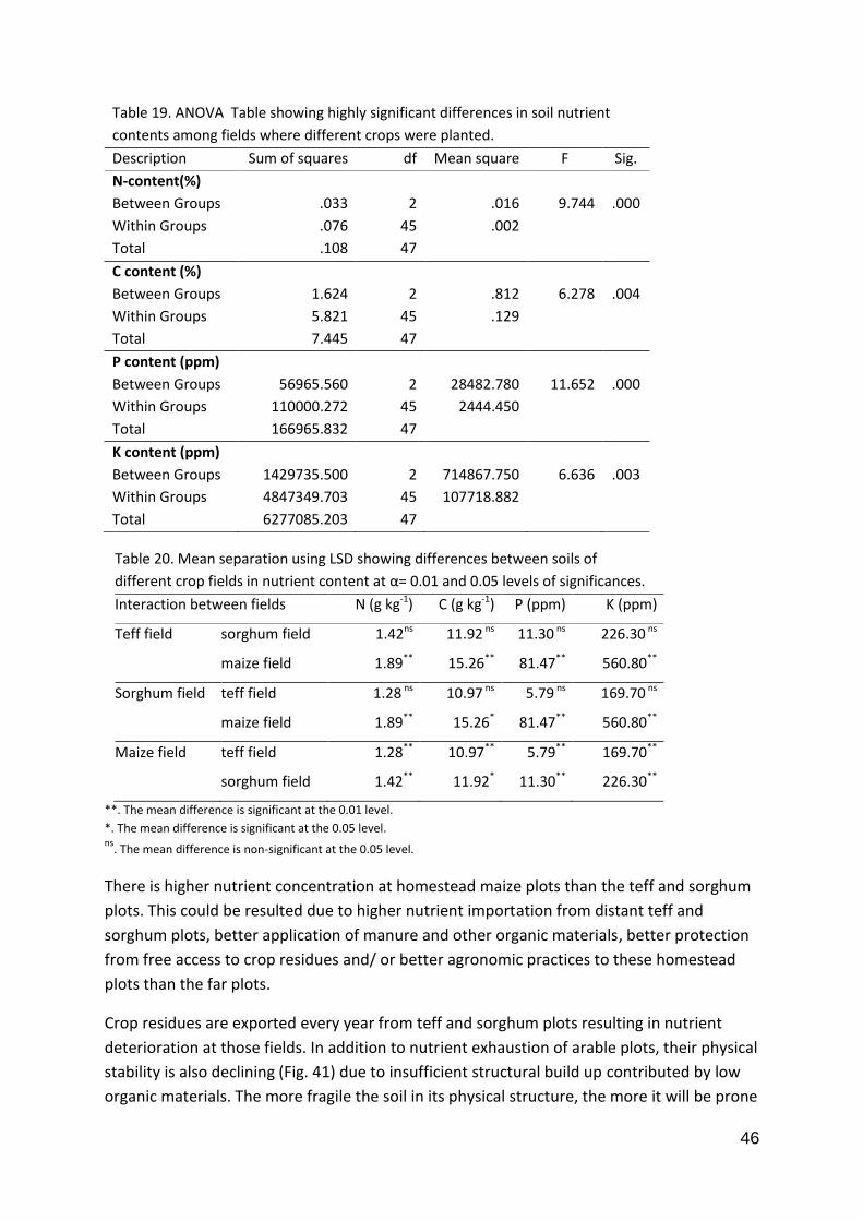
46
Table 19. ANOVA Table showing highly significant differences in soil nutrient
contents among fields where different crops were planted.
Description Sum of squares df Mean square F Sig.
N-content(%)
Between Groups .033 2 .016 9.744 .000
Within Groups .076 45 .002
Total .108 47
C content (%)
Between Groups 1.624 2 .812 6.278 .004
Within Groups 5.821 45 .129
Total 7.445 47
P content (ppm)
Between Groups 56965.560 2 28482.780 11.652 .000
Within Groups 110000.272 45 2444.450
Total 166965.832 47
K content (ppm)
Between Groups 1429735.500 2 714867.750 6.636 .003
Within Groups 4847349.703 45 107718.882
Total 6277085.203 47
Table 20. Mean separation using LSD showing differences between soils of
different crop fields in nutrient content at α= 0.01 and 0.05 levels of significances.
Interaction between fields N (g kg-1) C (g kg-1) P (ppm) K (ppm)
Teff field sorghum field 1.42ns 11.92 ns 11.30 ns 226.30 ns
maize field 1.89** 15.26** 81.47** 560.80**
Sorghum field teff field 1.28 ns 10.97 ns 5.79 ns 169.70 ns
maize field 1.89** 15.26* 81.47** 560.80**
Maize field teff field 1.28** 10.97** 5.79** 169.70**
sorghum field 1.42** 11.92* 11.30** 226.30**
**. The mean difference is significant at the 0.01 level.
*. The mean difference is significant at the 0.05 level. ns
. The mean difference is non-significant at the 0.05 level.
There is higher nutrient concentration at homestead maize plots than the teff and sorghum
plots. This could be resulted due to higher nutrient importation from distant teff and
sorghum plots, better application of manure and other organic materials, better protection
from free access to crop residues and/ or better agronomic practices to these homestead
plots than the far plots.
Crop residues are exported every year from teff and sorghum plots resulting in nutrient
deterioration at those fields. In addition to nutrient exhaustion of arable plots, their physical
stability is also declining (Fig. 41) due to insufficient structural build up contributed by low
organic materials. The more fragile the soil in its physical structure, the more it will be prone
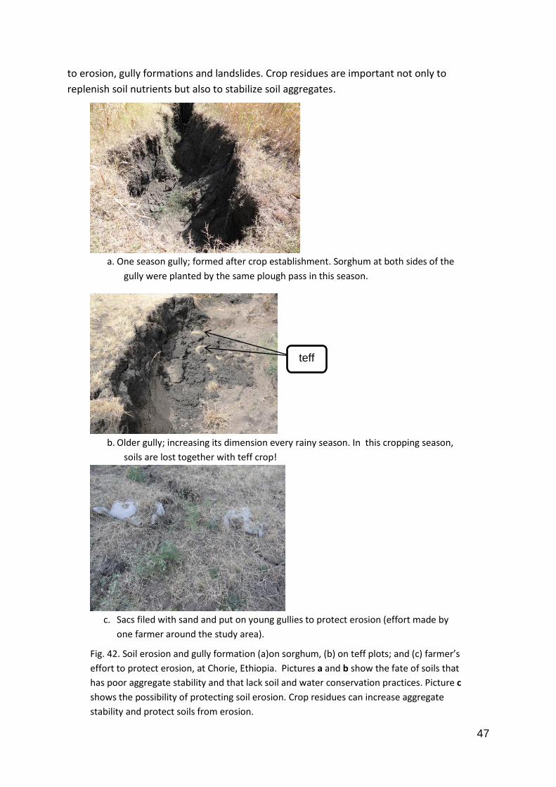
47
a. One season gully; formed after crop establishment. Sorghum at both sides of the
gully were planted by the same plough pass in this season.
b. Older gully; increasing its dimension every rainy season. In this cropping season,
soils are lost together with teff crop!
c. Sacs filed with sand and put on young gullies to protect erosion (effort made by
one farmer around the study area).
Fig. 42. Soil erosion and gully formation (a)on sorghum, (b) on teff plots; and (c) farmer’s
effort to protect erosion, at Chorie, Ethiopia. Pictures a and b show the fate of soils that
has poor aggregate stability and that lack soil and water conservation practices. Picture c
shows the possibility of protecting soil erosion. Crop residues can increase aggregate
stability and protect soils from erosion.
to erosion, gully formations and landslides. Crop residues are important not only to
replenish soil nutrients but also to stabilize soil aggregates.
Teff
teff
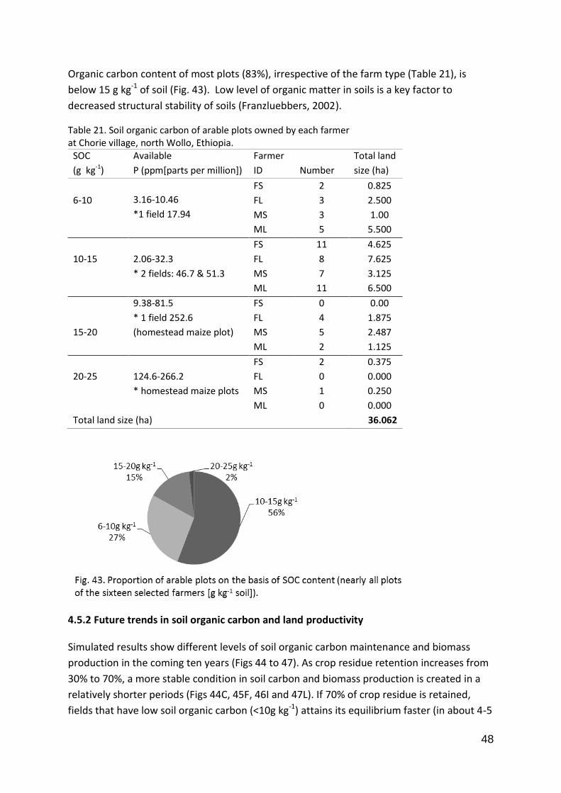
48
Organic carbon content of most plots (83%), irrespective of the farm type (Table 21), is
below 15 g kg-1 of soil (Fig. 43). Low level of organic matter in soils is a key factor to
decreased structural stability of soils (Franzluebbers, 2002).
Table 21. Soil organic carbon of arable plots owned by each farmer at Chorie village, north Wollo, Ethiopia.
SOC
(g kg-1)
Available
P (ppm[parts per million])
Farmer
ID Number
Total land
size (ha)
6-10
3.16-10.46
*1 field 17.94
FS 2 0.825
FL 3 2.500
MS 3 1.00
ML 5 5.500
10-15
2.06-32.3
* 2 fields: 46.7 & 51.3
FS 11 4.625
FL 8 7.625
MS 7 3.125
ML 11 6.500
15-20
9.38-81.5
* 1 field 252.6
(homestead maize plot)
FS 0 0.00
FL 4 1.875
MS 5 2.487
ML 2 1.125
20-25
124.6-266.2
* homestead maize plots
FS 2 0.375
FL 0 0.000
MS 1 0.250
ML 0 0.000
Total land size (ha) 36.062
4.5.2 Future trends in soil organic carbon and land productivity
Simulated results show different levels of soil organic carbon maintenance and biomass
production in the coming ten years (Figs 44 to 47). As crop residue retention increases from
30% to 70%, a more stable condition in soil carbon and biomass production is created in a
relatively shorter periods (Figs 44C, 45F, 46I and 47L). If 70% of crop residue is retained,
fields that have low soil organic carbon (<10g kg-1) attains its equilibrium faster (in about 4-5
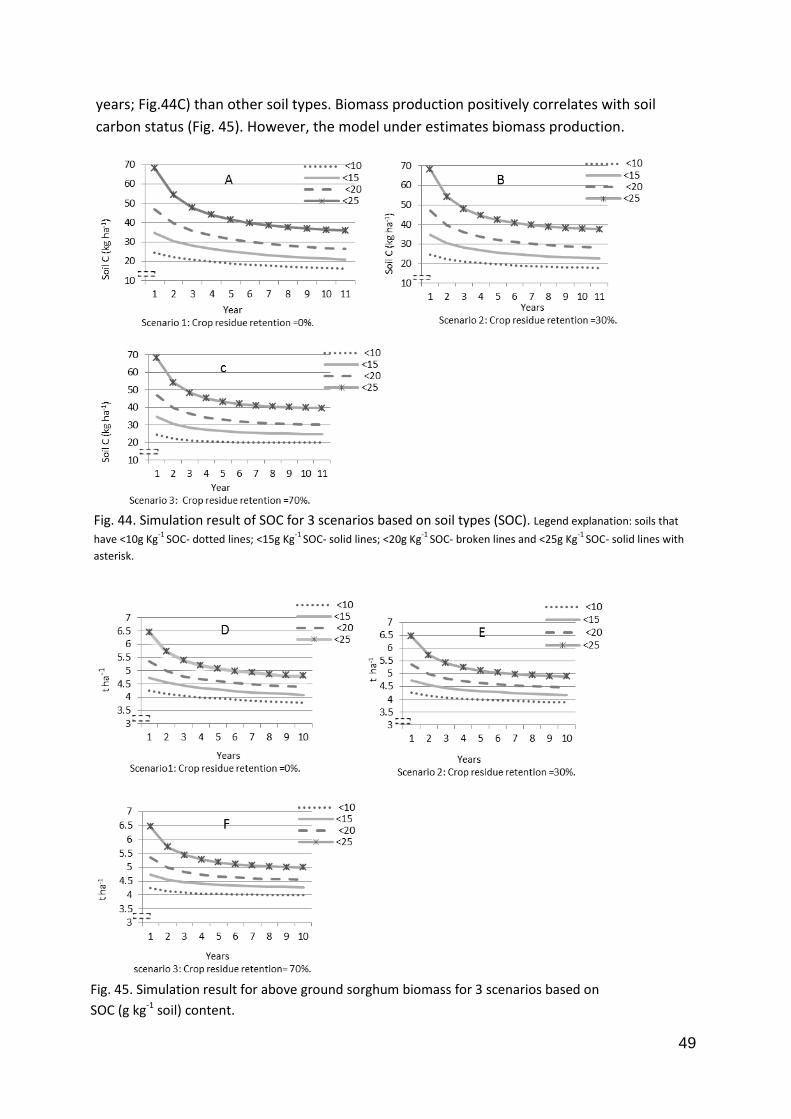
49
years; Fig.44C) than other soil types. Biomass production positively correlates with soil
carbon status (Fig. 45). However, the model under estimates biomass production.
Fig. 45. Simulation result for above ground sorghum biomass for 3 scenarios based on
SOC (g kg-1 soil) content.
Fig. 44. Simulation result of SOC for 3 scenarios based on soil types (SOC). Legend explanation: soils that
have <10g Kg-1
SOC- dotted lines; <15g Kg-1
SOC- solid lines; <20g Kg-1
SOC- broken lines and <25g Kg-1
SOC- solid lines with
asterisk.
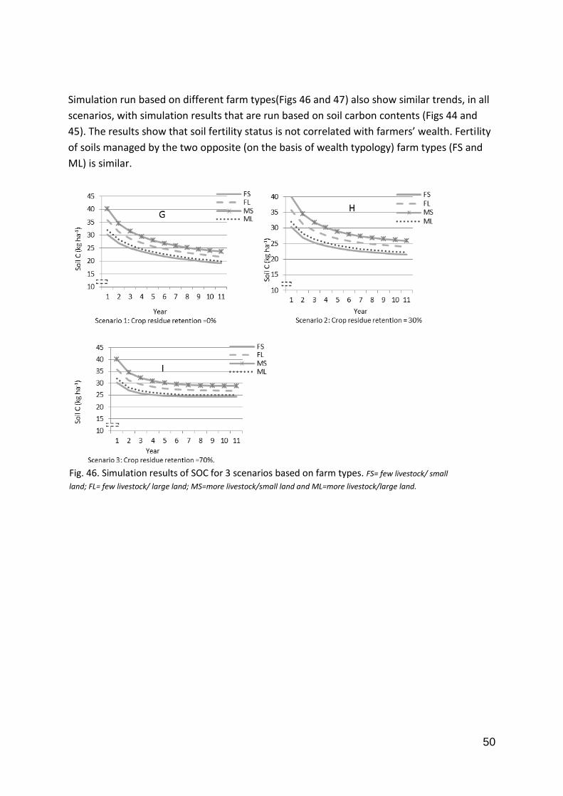
50
Simulation run based on different farm types(Figs 46 and 47) also show similar trends, in all
scenarios, with simulation results that are run based on soil carbon contents (Figs 44 and
45). The results show that soil fertility status is not correlated with farmers’ wealth. Fertility
of soils managed by the two opposite (on the basis of wealth typology) farm types (FS and
ML) is similar.
Fig. 46. Simulation results of SOC for 3 scenarios based on farm types. FS= few livestock/ small
land; FL= few livestock/ large land; MS=more livestock/small land and ML=more livestock/large land.
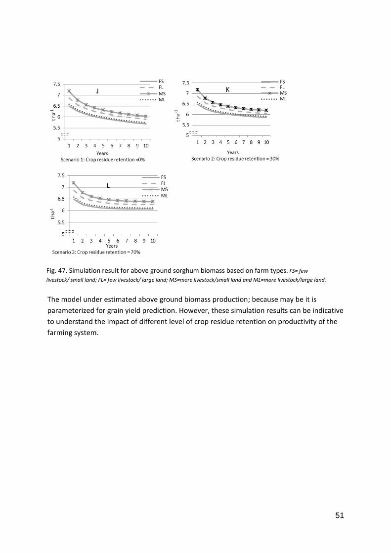
51
The model under estimated above ground biomass production; because may be it is
parameterized for grain yield prediction. However, these simulation results can be indicative
to understand the impact of different level of crop residue retention on productivity of the
farming system.
Fig. 47. Simulation result for above ground sorghum biomass based on farm types. FS= few
livestock/ small land; FL= few livestock/ large land; MS=more livestock/small land and ML=more livestock/large land.

52
53
Chapter 5. Discussion
5.1 Crop residues utilization
At Chorie, more than 90% of teff straw, 74% of sorghum stover and 81% of maize stover
are used for livestock feed through stubble grazing and stall feeding (Figs 26,27 and 28). The
result is in line with the finding of de Leeuw (1997). Crop residues use for home energy is
almost similar for all farm types (11-15%; Fig. 27). The result indicates that extremely low
amounts of crop residues are left for soil organic matter enhancement; probably not more
than the root biomass (Tables 19 and 20). Simulation results (Figs 42, 43, 44A, B and 46G, H)
and previous works already explained in Chapter 2 reveal that severe crop residues removal
results in degradation of soil physical and chemical characteristics. One strategy to retain
sufficient crop residues and produce satisfactory feed could be increasing biomass
production through high yielding varieties.
For teff crop, the improved variety, Sikuar magna, has many superior qualities to be
selected to the system. It produces higher biomass, has good home and market demand,
and matures early next to Bunign (Annexes 4 and 7). However, for sorghum crop, the local
varieties Jigurtie and Abola produce higher biomass than the improved Wedhakir varieties.
Therefore, from local sorghum varieties, farmers can get higher biomass production, good
feed, food and market values; these varieties have low nitrogen content and digestibility
percentages but it can be compensated by higher biomass yield. For Chorie farmers,
biomass production is the priority criteria for a variety to be selected to satisfy feed, food, as
well as organic inputs to their soils. Due to rain uncertainty, farmers greatly shifted to early
maturing but low yielding sorghum varieties. This means that the probability of losing higher
yields at good production seasons is high. Extension workers should be careful in advising
farmers which variety they should use in order to maximize advantages from these varieties.
Quantity of crop residues can be adequately increased through high yielding varieties
provided that there are no limiting factors. Yet, scientists (e.g. Williams et al., 1997) argue
for digestibility of thicker and stronger stovers from high yielding sorghum varieties.
Digestibility analysis for stem parts of different sorghum varieties show none-significant
difference at upper and middle stem parts; differences are significant only at lower stem
parts(Tables 13 and 14). Based on this result, farmers can allocate upper parts for livestock
feed and lower parts for soil amendment activities.
Strong feed shortages from pasture/rangelands and firewood shortages from woodlots in
the area forced farmers to depend on crop residues for their livestock feed; and to use it as
energy supply. This situation leads to strong tradeoffs between short term benefits and long
term farm sustainability. These negative trade-offs can be improved by retaining more crop
residues (up to 70% or even higher when possible; Figs 44C and 46I; Tittonell et al., 2008) in
54
the field. However due consideration should be given to ensure higher percentage of
incorporating it to the soil.
The competing use of crop residues for livestock feed, fuel and soil fertility management
activities may be improved through various efforts, such as encouraging farmers to plant
leguminous fodder trees, multipurpose trees (Oluyede et al., 2007) around homesteads,
riversides and field boarders to reduce use of crop residues for fuel and construction
materials. Multipurpose trees can be used for livestock feed, they can fix atmospheric
nitrogen and are also fuel sources (Unger et al.,1997). Encouraging farmers’ indigenous tree
and shrub management practices like shade trees in their fields, contour hedges, live fences,
wood lots etc. are likely to contribute a lot in any intervention strategy (Kindu et al., 2009).
Trees increase water infiltration, protect erosion, provide feed to livestock, nutrients to
soils, fire wood for energy, logs for construction materials and many more environmental
benefits.
5.2 Manure utilization
In the study area farmers need technical support to improve their manure allocation for
fertilizer. They allocate only about 28% to fertilize their small size homestead maize plot;
teff and sorghum plots receive no manure. More than 46% of manure is used for fuel and
about 26% is left un-used (Fig. 33A). There is small difference among farm types in manure
allocation (Fig. 33B). FL and MS farm types apply lower than FS and ML farm types. This
variation could be due to labor availability, land tenure or field distance from home. In any
case farmers use relatively low proportion of manure as fertilizer; yet, they complain that it
resulted weed infestation and crop burning effects. This could be due to low quality of
manure in its nutrient content as findings ( e.g. Tittonell et al., 2008; Giller et al., 2011)
already confirmed this case, and /or it could be due to inappropriate time and method of
application (Thomsen,2005). Therefore, it is very important to provide technical support to
farmers to properly utilize manure at least in their homestead plots. Interventions for soil
fertility management measures can be started with low cost resources like manure and
other organic materials that are available at the hands of farmers.
Many scientists (e.g. Zingore, 2006; Zingore et al., 2007a;b; Bationo et al., 2007; Okumu et
al., 2011) reported that soil fertility gradient have developed due to farmers’ preferential
application of organic and chemical fertilizers to homestead plots. In the study area, the
settlement location is the most important factor due to difficulties to transport the bulky
manure to the far main crop lands. Villagers live at higher elevation following a mountain
contour belt. This could be good strategy to avoid flood and mud challenges during heavy
rainy season but it creates considerable distance between crop lands and homesteads. The
distance negatively affects the timeliness of agronomic management practices. There is
hardly any nutrient transport from home to these far arable plots except seeds. Extreme
removal of crop residues for feed, fuel and other purposes coupled with no manure or
55
chemical fertilizer application to replenish nutrients exported through crop production is
the characteristic of the current farming system at Chorie. Resettlement of farmers close to
their main crop plots may help to improve their soil fertility management activities.
Nutrient contents of plots managed by different farm types are statistically similar; there are
no significant differences in C, N, P and K contents (Annex 8) among plots of farm types,
even at the homestead plots. Though there are differences among farm types in the number
of livestock (that affect amount of crop residues collection and manure), land holding,
gender, labor availability and so on, nutrient status of their soils are not statistically
different. Farmers who have livestock may apply more manure than those who do not have
livestock, yet the effect is not explained in the soil fertility status. This could be due to poor
manure application practice and/or poor quality of manure to enhance soil fertility at least
at homestead plots where farmers usually apply manure. Low quality of manure is resulted
because of poor handling and storage practices (Fig. 11; Powell and Williams, 1993; Nzuma
et al., 1997; Rufino, 2008; Tittonell et al., 2008; Giller et al., 2011).
5.3 Crop residues and manure management practices of farm types
Generally, there are no differences among farm types in soil fertility management practices.
Crop residues and in-situ dung collection from arable plots as well as crop residues and
manure allocation strategies are similar. However, quantity of allocating these resources to
various uses differ among farm types depending on the number of livestock owned, land
tenure condition and labor availability. In addition to these, the following are other multiple
factors that create differences.
1) Social: farmers settle far from their main crop lands. They need to transport crop
residues from field to homestead. In this case, in addition to labor, gender and age
variability create differences in the amount of transported crop residues, management
and decisions on the allocation.
2) Environmental: Amount and distribution of rainfall affects variety selection and hence
total biomass production, as well as livestock productivity (Fig. 35). High yielding
sorghum varieties are late maturing ones and require sufficient moisture in April with
subsequent topping. Early maturing varieties are low in their biomass yield (Fig. 18).
The less biomass production in the cropping season, the sever crop residue removal for
stall feeding will be. Farmers are forced to shift their energy source from woods to crop
residues because of declining woodlots to supply firewood (Figs 38 and 40).
3) Economic: farmers hire labor for peak land activities like harvesting, and rent camel for
transporting crop residues. Moreover, selling crop residues also depends on economic
performance of farmers in such a way that poor farmers collect as many residues as
possible for sale whereas richer farmers collect residues mostly for their own demands.
4) Lack of legal protection: Anybody has free access to arable plots after crop harvest,
people living in the surrounding collect crop residues for fuel and other purposes, and
56
allow livestock for free grazing. Everybody tries to maximize its share; this competition
results in severe depletion of soil organic matter.
5) Lack of alternative technologies: Feed technologies (different annual and perennials
feed plants), alternative energy sources like biofuel, wood lots etc. are not tried yet.
Soil and water conservation practices are very limited to highly degraded areas. The
situation alerts quick and strong intervention to ensure sustainable farm productivity
and improve farmers’ livelihood in the area.
5.4 Limitation of the study
Data on socio-economic aspects and resource allocations are collected based on farmers’
estimation through interviews. Even though thorough discussions were made with farmers
and care was taken during farmers’ estimation, precision on values are still lacking. Yield
samples are taken from crops that are planted at farmers’ fields of different soils, that
received different agronomic practices. Hence, comparison for different traits may not
represent potential differences of varieties. Furthermore, the number of replica for varieties
is not equal due to random selection of farmers. Results for some varieties are averages of
8, for others are averages of 4 or 3 and for others average of only one plot samples. So
results in this report could be indicative but may not be precise.
57
Chapter 6. Conclusion and recommendation
It is important to maintain crop diversity to increase the chance of farmers’ flexibility
according to climatic and economic influences. All local varieties should not be
substituted by improved ones; because, not all improved varieties are suitable to
production objectives of a given area. Farmers’ priority should be considered when
providing seeds to them. Accordingly, the improved teff variety, Sikuar magna, and
the local sorghum varieties, Jigurtie and Abola, are better varieties for Chorie
farming system.
The current method of crop residue storage, especially sorghum and maize residues
need processing activities (at least chopping down) to facilitate intake by livestock.
Furthermore, attention should be given to storage places /conditions to protect crop
residues from extended solar radiation and moisture entrance that deteriorate its
quality and quantity.
There is no difference among farm types in soil fertility management strategy and the
use of crop residues. Variations are rather on decision makings due to climatic,
social, gender, economic and institutional influences.
Gender of the head of a household is key element to resource management in the
study area; legal document concerning land renting or sharing agreements to protect
female and aged farmers from personal (tiller) exploitation, and to safeguard land
productivity is very important to female headed and aged households.
Current crop residue and manure management practices are negatively affecting soil
carbon stock and land productivity. To restore the declining soil carbon and ensure
sustainable land productivity, sufficiently higher percentage of crop residues need to
be retained in the soil.
The study area needs strong interventions about alternative livestock feeds,
alternative energy sources, rain water harvesting (at least for homestead gardening),
efficient use of manure, legal support to crop residues property right and so on.
Although models developed elsewhere can be adapted to predict crops having similar
characteristics, site variations could create differences in crop performances and
biophysical processes; which may limit the prediction power of models
parameterized at other localities. Primary data for specific condition is important to
generate reliable prediction from models.

58
59
List of references
Abegaz, A., van Keulen, H., Oosting, S.J., 2007. Feed resources, livestock production and soil
carbon dynamics in Teghane, Northern Highlands of Ethiopia. Agricultural Systems, 94,
pp.391-404.
Adrian, R.E., 1997. Technological constraints and opportunities in relation to class of
livestock and production objectives. In: C. Renard, ed. 1997. Crop residues in
sustainable mixed crop/livestock farming system.UK: CAB International, pp.7-24.
Aggarwal, R. K., Praveen, K., Power J.F., 1997. Use of crop residue and manure to conserve
water and enhance nutrient availability and pearl millet yields in an arid tropical
region. Soil & Tillage Research, 41(1-2), pp.43-51.
Anderson, F. M., 1987. Farmer circumstances in Ethiopia and the improvement of animal
feed resources. ILCA, Addis Ababa, Ethiopia. Available on
http://www.ilri.cgiar.org/InfoServ/Webpub/fulldocs/X5548E/X5548E0K.HTM
[Accessed 1o June2010).
Bationo, A., Kihara, J., Vanlauwe, B., Waswa, B., Kimetu, J., 2007. Soil organic carbon
dynamics, functions and management in West African agro-ecosystems. Agricultural
Systems, 94, pp.13-25.
Batten, G.D., 1998. Plant analysis using near infrared reflectance spectroscopy: the potential
and the limitations. Australian Journal of Experimental Agriculture, 38 (7), pp. 697-
706.
Beauchamp, E. G. and Voroney, R. P., 1994. Crop carbon contribution to the soil with
different cropping and livestock systems. Journal of Soil and Water Conservation,
49(2), pp. 205-209.
Benjamin, J. G., Halvorson, A. D, Nielsen, D.C. and Mikha, M.M., 2010. Crop management
effects on crop residue production and changes in soil organic carbon in the central
great plains. Agronomy Journal, 102(3), pp. 990-997.
Berhanu, G., Pender, J., and Girmay, T., 2002. Collective action for grazing land management
in mixed crop-livestock systems in the highlands of northern Ethiopia. In: ILRI (Nairobi,
Kenya), Socio- economics and policy research working paper, 42, p.28.
Dagnachew A.Y., 2008. Exploring options to model resource limited production of Pear Millet
and sorghum in Mali. MSc. Wageningen: Wageningen university, The Netherlands.
De Leeuw, P.N., 1997. Crop residues in tropical Africa: trends in supply, demand and use. In:
C. Renard, ed. 1997. Crop residues in sustainable mixed crop/livestock farming system.
UK:CAB International, pp.41-77.
Di Falco, S., Mintewab, B., Mahmud, Y., 2010. Seeds for livelihood: crop biodiversity and
food production in Ethiopia. Ecological Economics, 69, pp.1695–1702.
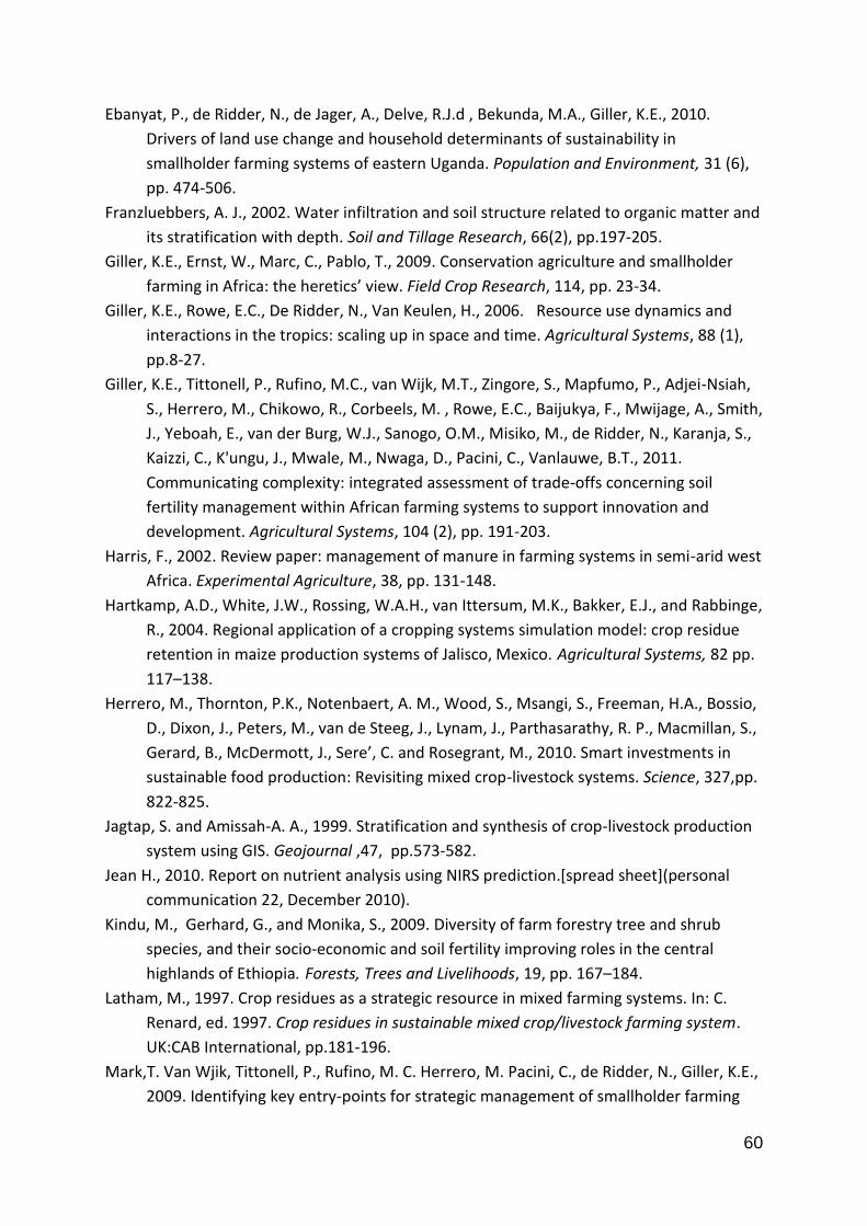
60
Ebanyat, P., de Ridder, N., de Jager, A., Delve, R.J.d , Bekunda, M.A., Giller, K.E., 2010.
Drivers of land use change and household determinants of sustainability in
smallholder farming systems of eastern Uganda. Population and Environment, 31 (6),
pp. 474-506.
Franzluebbers, A. J., 2002. Water infiltration and soil structure related to organic matter and
its stratification with depth. Soil and Tillage Research, 66(2), pp.197-205.
Giller, K.E., Ernst, W., Marc, C., Pablo, T., 2009. Conservation agriculture and smallholder
farming in Africa: the heretics’ view. Field Crop Research, 114, pp. 23-34.
Giller, K.E., Rowe, E.C., De Ridder, N., Van Keulen, H., 2006. Resource use dynamics and
interactions in the tropics: scaling up in space and time. Agricultural Systems, 88 (1),
pp.8-27.
Giller, K.E., Tittonell, P., Rufino, M.C., van Wijk, M.T., Zingore, S., Mapfumo, P., Adjei-Nsiah,
S., Herrero, M., Chikowo, R., Corbeels, M. , Rowe, E.C., Baijukya, F., Mwijage, A., Smith,
J., Yeboah, E., van der Burg, W.J., Sanogo, O.M., Misiko, M., de Ridder, N., Karanja, S.,
Kaizzi, C., K'ungu, J., Mwale, M., Nwaga, D., Pacini, C., Vanlauwe, B.T., 2011.
Communicating complexity: integrated assessment of trade-offs concerning soil
fertility management within African farming systems to support innovation and
development. Agricultural Systems, 104 (2), pp. 191-203.
Harris, F., 2002. Review paper: management of manure in farming systems in semi-arid west
Africa. Experimental Agriculture, 38, pp. 131-148.
Hartkamp, A.D., White, J.W., Rossing, W.A.H., van Ittersum, M.K., Bakker, E.J., and Rabbinge,
R., 2004. Regional application of a cropping systems simulation model: crop residue
retention in maize production systems of Jalisco, Mexico. Agricultural Systems, 82 pp.
117–138.
Herrero, M., Thornton, P.K., Notenbaert, A. M., Wood, S., Msangi, S., Freeman, H.A., Bossio,
D., Dixon, J., Peters, M., van de Steeg, J., Lynam, J., Parthasarathy, R. P., Macmillan, S.,
Gerard, B., McDermott, J., Sere’, C. and Rosegrant, M., 2010. Smart investments in
sustainable food production: Revisiting mixed crop-livestock systems. Science, 327,pp.
822-825.
Jagtap, S. and Amissah-A. A., 1999. Stratification and synthesis of crop-livestock production
system using GIS. Geojournal ,47, pp.573-582.
Jean H., 2010. Report on nutrient analysis using NIRS prediction.[spread sheet](personal
communication 22, December 2010).
Kindu, M., Gerhard, G., and Monika, S., 2009. Diversity of farm forestry tree and shrub
species, and their socio-economic and soil fertility improving roles in the central
highlands of Ethiopia. Forests, Trees and Livelihoods, 19, pp. 167–184.
Latham, M., 1997. Crop residues as a strategic resource in mixed farming systems. In: C.
Renard, ed. 1997. Crop residues in sustainable mixed crop/livestock farming system.
UK:CAB International, pp.181-196.
Mark,T. Van Wjik, Tittonell, P., Rufino, M. C. Herrero, M. Pacini, C., de Ridder, N., Giller, K.E.,
2009. Identifying key entry-points for strategic management of smallholder farming
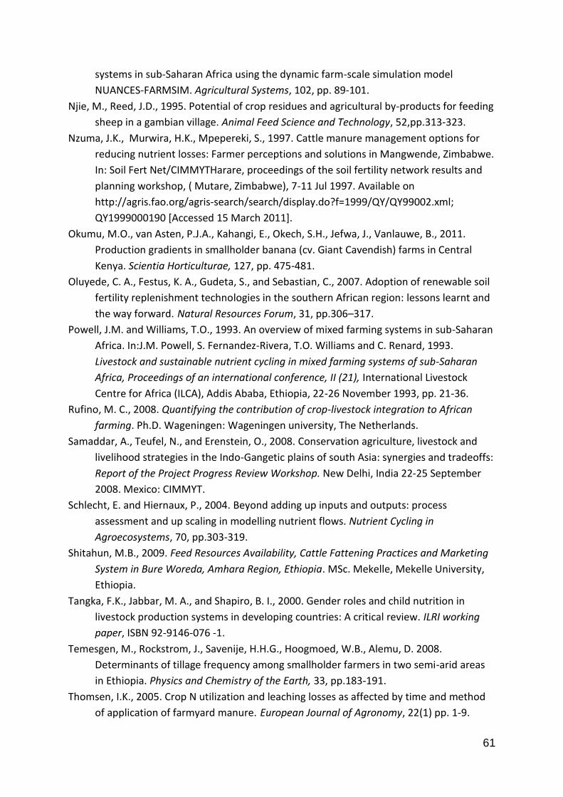
61
systems in sub-Saharan Africa using the dynamic farm-scale simulation model
NUANCES-FARMSIM. Agricultural Systems, 102, pp. 89-101.
Njie, M., Reed, J.D., 1995. Potential of crop residues and agricultural by-products for feeding
sheep in a gambian village. Animal Feed Science and Technology, 52,pp.313-323.
Nzuma, J.K., Murwira, H.K., Mpepereki, S., 1997. Cattle manure management options for
reducing nutrient losses: Farmer perceptions and solutions in Mangwende, Zimbabwe.
In: Soil Fert Net/CIMMYTHarare, proceedings of the soil fertility network results and
planning workshop, ( Mutare, Zimbabwe), 7-11 Jul 1997. Available on
http://agris.fao.org/agris-search/search/display.do?f=1999/QY/QY99002.xml;
QY1999000190 [Accessed 15 March 2011].
Okumu, M.O., van Asten, P.J.A., Kahangi, E., Okech, S.H., Jefwa, J., Vanlauwe, B., 2011.
Production gradients in smallholder banana (cv. Giant Cavendish) farms in Central
Kenya. Scientia Horticulturae, 127, pp. 475-481.
Oluyede, C. A., Festus, K. A., Gudeta, S., and Sebastian, C., 2007. Adoption of renewable soil
fertility replenishment technologies in the southern African region: lessons learnt and
the way forward. Natural Resources Forum, 31, pp.306–317.
Powell, J.M. and Williams, T.O., 1993. An overview of mixed farming systems in sub-Saharan
Africa. In:J.M. Powell, S. Fernandez-Rivera, T.O. Williams and C. Renard, 1993.
Livestock and sustainable nutrient cycling in mixed farming systems of sub-Saharan
Africa, Proceedings of an international conference, II (21), International Livestock
Centre for Africa (ILCA), Addis Ababa, Ethiopia, 22-26 November 1993, pp. 21-36.
Rufino, M. C., 2008. Quantifying the contribution of crop-livestock integration to African
farming. Ph.D. Wageningen: Wageningen university, The Netherlands.
Samaddar, A., Teufel, N., and Erenstein, O., 2008. Conservation agriculture, livestock and
livelihood strategies in the Indo-Gangetic plains of south Asia: synergies and tradeoffs:
Report of the Project Progress Review Workshop. New Delhi, India 22-25 September
2008. Mexico: CIMMYT.
Schlecht, E. and Hiernaux, P., 2004. Beyond adding up inputs and outputs: process
assessment and up scaling in modelling nutrient flows. Nutrient Cycling in
Agroecosystems, 70, pp.303-319.
Shitahun, M.B., 2009. Feed Resources Availability, Cattle Fattening Practices and Marketing
System in Bure Woreda, Amhara Region, Ethiopia. MSc. Mekelle, Mekelle University,
Ethiopia.
Tangka, F.K., Jabbar, M. A., and Shapiro, B. I., 2000. Gender roles and child nutrition in
livestock production systems in developing countries: A critical review. ILRI working
paper, ISBN 92-9146-076 -1.
Temesgen, M., Rockstrom, J., Savenije, H.H.G., Hoogmoed, W.B., Alemu, D. 2008.
Determinants of tillage frequency among smallholder farmers in two semi-arid areas
in Ethiopia. Physics and Chemistry of the Earth, 33, pp.183-191.
Thomsen, I.K., 2005. Crop N utilization and leaching losses as affected by time and method
of application of farmyard manure. European Journal of Agronomy, 22(1) pp. 1-9.
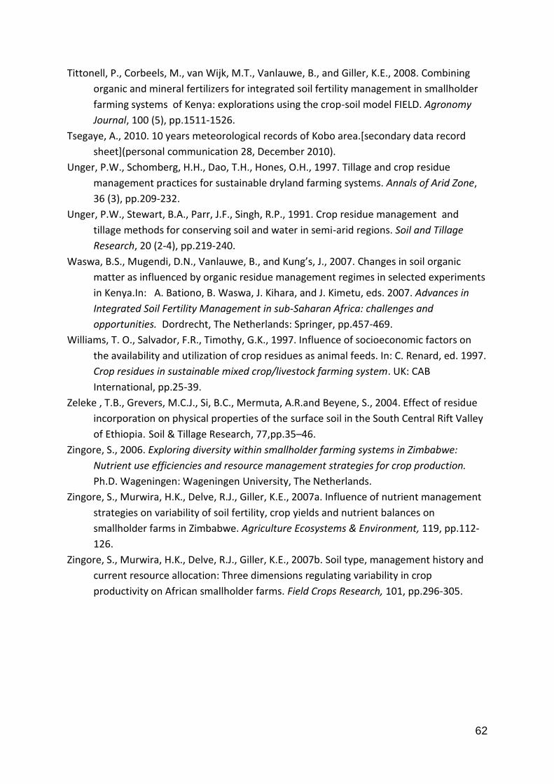
62
Tittonell, P., Corbeels, M., van Wijk, M.T., Vanlauwe, B., and Giller, K.E., 2008. Combining
organic and mineral fertilizers for integrated soil fertility management in smallholder
farming systems of Kenya: explorations using the crop-soil model FIELD. Agronomy
Journal, 100 (5), pp.1511-1526.
Tsegaye, A., 2010. 10 years meteorological records of Kobo area.[secondary data record
sheet](personal communication 28, December 2010).
Unger, P.W., Schomberg, H.H., Dao, T.H., Hones, O.H., 1997. Tillage and crop residue
management practices for sustainable dryland farming systems. Annals of Arid Zone,
36 (3), pp.209-232.
Unger, P.W., Stewart, B.A., Parr, J.F., Singh, R.P., 1991. Crop residue management and
tillage methods for conserving soil and water in semi-arid regions. Soil and Tillage
Research, 20 (2-4), pp.219-240.
Waswa, B.S., Mugendi, D.N., Vanlauwe, B., and Kung’s, J., 2007. Changes in soil organic
matter as influenced by organic residue management regimes in selected experiments
in Kenya.In: A. Bationo, B. Waswa, J. Kihara, and J. Kimetu, eds. 2007. Advances in
Integrated Soil Fertility Management in sub-Saharan Africa: challenges and
opportunities. Dordrecht, The Netherlands: Springer, pp.457-469.
Williams, T. O., Salvador, F.R., Timothy, G.K., 1997. Influence of socioeconomic factors on
the availability and utilization of crop residues as animal feeds. In: C. Renard, ed. 1997.
Crop residues in sustainable mixed crop/livestock farming system. UK: CAB
International, pp.25-39.
Zeleke , T.B., Grevers, M.C.J., Si, B.C., Mermuta, A.R.and Beyene, S., 2004. Effect of residue
incorporation on physical properties of the surface soil in the South Central Rift Valley
of Ethiopia. Soil & Tillage Research, 77,pp.35–46.
Zingore, S., 2006. Exploring diversity within smallholder farming systems in Zimbabwe:
Nutrient use efficiencies and resource management strategies for crop production.
Ph.D. Wageningen: Wageningen University, The Netherlands.
Zingore, S., Murwira, H.K., Delve, R.J., Giller, K.E., 2007a. Influence of nutrient management
strategies on variability of soil fertility, crop yields and nutrient balances on
smallholder farms in Zimbabwe. Agriculture Ecosystems & Environment, 119, pp.112-
126.
Zingore, S., Murwira, H.K., Delve, R.J., Giller, K.E., 2007b. Soil type, management history and
current resource allocation: Three dimensions regulating variability in crop
productivity on African smallholder farms. Field Crops Research, 101, pp.296-305.
63
Annexes
Annex 1. Population and land availability at Chorie village Description Quantity Description Quantity
Total population 515 Total house hold 103
Cultivated land (ha) 618 Female head house hold 25
Rain fed 618 House hold without dairy 50
Irrigated 0
Annex 2. Parameters used to calibrate the model FIELD a. Site specific parameters
No. Description Value used
1 Maximum relative decomposition rate of residue C 0.8
2 “ “ “ “ “ root C 0.8
3 “ “ “ “ “ active C 0.69
4 “ “ “ “ “ soil C 0.2
5 Growth efficiency of microbes (immobilization of N b y active organic matter)
0.6
6 C-N ratio active C pool (kg C ha-1
)/(Kg N ha-1
) 8
7 C-P “ “ “ “ “ 40
8 Humification factor 0.25
9 Relative amount of decomposed soil organic matter that re-enters the soil organic matter pool
0.2
10 Fraction of C originally in the soil C pool 0.9
11 Fraction of inert C in the soil C pool 0.55
12 Seasonal relative turnover of inert C pool 0.001
13 Rain fall (mm season-1
) 550
14 Water capture efficiency 0.20
15 Water conversion efficiency 88.7
16 Correction factor for relative decomposition rate of active organic matter 1
17 “ “ “ “ “ soil organic matter 1
18 “ “ “ “ “ residues 1
19 “ “ “ “ “ residues 1
20 Maximum soil organic matter level (kg C ha-1
) 30,000
b. Soil specific parameters
No. Description Value used
1 Soil texture (%) Clay Sand Silt
6 52 42
2 Soil organic carbon (g kg-1
) 4.7
3 Total soil N 0.4
4 Exchangeable P 9
5 “ K 170
6 “ Ca 1.5
7 “ Mg 2.1
8 ECEC 4.5
9 PH 6.6
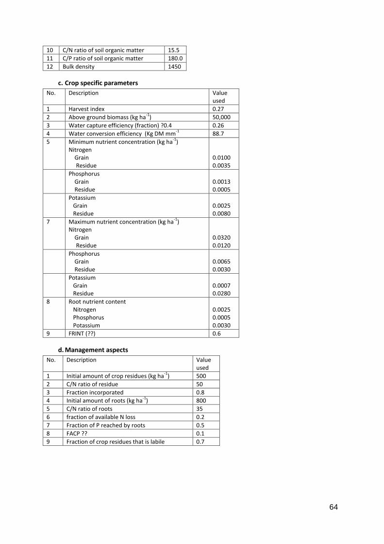
64
10 C/N ratio of soil organic matter 15.5
11 C/P ratio of soil organic matter 180.0
12 Bulk density 1450
c. Crop specific parameters
No. Description Value used
1 Harvest index 0.27
2 Above ground biomass (kg ha-1
) 50,000
3 Water capture efficiency (fraction) ?0.4 0.26
4 Water conversion efficiency (Kg DM mm-1
88.7
5 Minimum nutrient concentration (kg ha-1
) Nitrogen Grain Residue
0.0100 0.0035
Phosphorus Grain Residue
0.0013 0.0005
Potassium Grain Residue
0.0025 0.0080
7 Maximum nutrient concentration (kg ha-1
) Nitrogen Grain Residue
0.0320 0.0120
Phosphorus Grain Residue
0.0065 0.0030
Potassium Grain Residue
0.0007 0.0280
8 Root nutrient content Nitrogen Phosphorus Potassium
0.0025 0.0005 0.0030
9 FRINT (??) 0.6
d. Management aspects
No. Description Value used
1 Initial amount of crop residues (kg ha-1
) 500
2 C/N ratio of residue 50
3 Fraction incorporated 0.8
4 Initial amount of roots (kg ha-1
) 800
5 C/N ratio of roots 35
6 fraction of available N loss 0.2
7 Fraction of P reached by roots 0.5
8 FACP ?? 0.1
9 Fraction of crop residues that is labile 0.7

65
Annex 3. Questionnaire used for socio-economic data collection
Household level survey: Crop residue and manure use in smallholder crop-livestock systems
The objective of this survey is to obtain a better understanding on farmers’ decisions related to crop residue
and manure management, and feeding strategies. Data collected here will be confidentially kept and reports
will not make reference to individual cases explicitly.
1. HOUSEHOLD GENERAL DATA
1.1. Identification: if possible, please add the coordinates of the homestead.
1.2. Household head: main information of the household head
a. hh head name ___________________ b. hh head father’s name _________________
c. hh head gender _____ (1) De jure female;
(2)
De facto female; (3) Male
d. hh head age ____ years old. e. hh head years in the village __ years f. Phone no. _____________
Number of years of education* of the: g. Head household _____ h. Leading female/wife _____
* It includes both formal/informal.
1.3. Household members: number and age of member including household head.
1. Female 2. Male 1. Female 2. Male
< 6 years old 6 – 9 years old
10 – 15 years old 15 - 60 years old
> 60 years old
1.4. Decisions: who take the decisions in the household (1) female, (2) male; (3) joint; (4) other
Decision on: Responsible
Main crops selection and management
Cash crops selection and management
Use of crop residues
Selection and management of small ruminants
Selection and management of large ruminants
1.5. Labor availability: is here a problem? Why?
_____________________________________________________________________________________________
2. ASSETS, ACCESSIBILITY & FOOD
2.1. Assets and services - (0) No; (1) Yes
Mobile phone _______ Radio ________ Region specific (transport) _____
2.2. Saving strategies: Is the household engaged in savings? ___ (0) No; (1) Yes. If yes, how? ____ (1) banks; (2) livestock; (3) property, Land (4) other way_______
2.3. Net food: How many months can you consume the main staple food (cereals) you produce in:
2.4. Food source: if yours is finished, how do you normally obtain extra staple food (cereals)? ___ 0) no need; (1) purchase food; (2) subsidised/food aid; (3) given by others; (4) other __________
2.5. Food-aid: In how many years did you need food-aid during the last 10 years? ____ years
3. LAND & CROPS Agricultural seasons: don’t ask this to the farmer, please use
the ones identified in the village survey
Village______________
a. Place of interview ____________________ (1) Homestead; (2) other, name: ______________________________
Coordinates homestead b. N/S ___________ c. E __________ d. Altitude __________masl
A year of average rainfall? ____ months A year of low rainfall? ____ months
Duration of season 1st Season 2nd Season 3rd Season
First – last month July – Sept. Oct. – Dec. Janu.- June
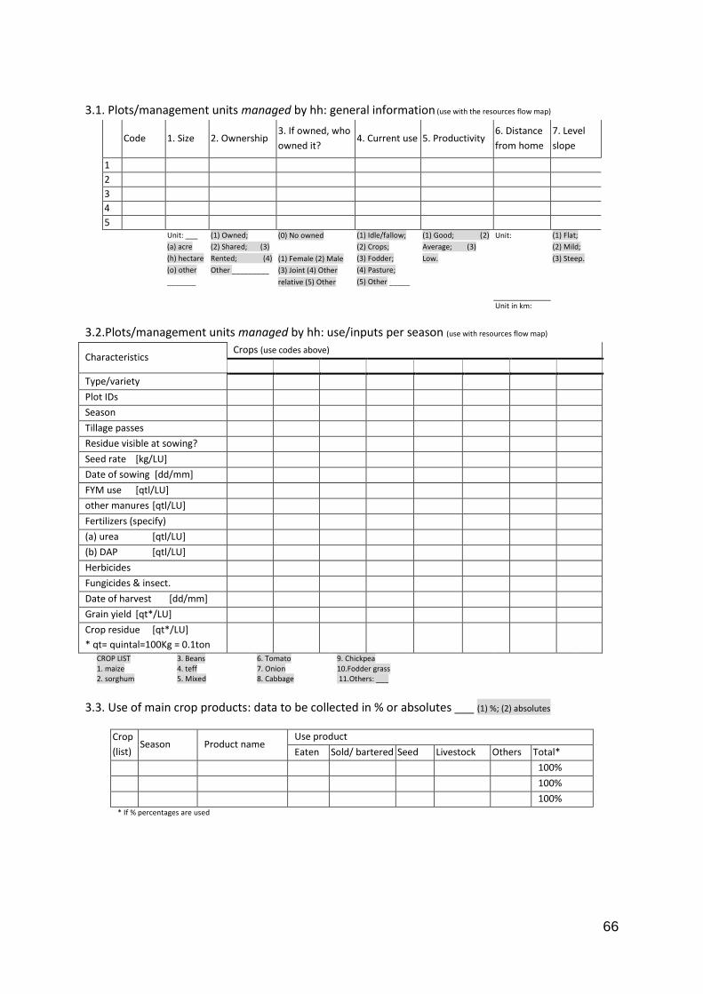
66
3.1. Plots/management units managed by hh: general information (use with the resources flow map)
Code 1. Size 2. Ownership 3. If owned, who
owned it? 4. Current use 5. Productivity
6. Distance
from home
7. Level
slope
1
2
3
4
5 Unit: ___
(a) acre
(h) hectare
(o) other
_______
(1) Owned;
(2) Shared; (3)
Rented; (4)
Other _________
(0) No owned
(1) Female (2) Male
(3) Joint (4) Other
relative (5) Other
(1) Idle/fallow;
(2) Crops;
(3) Fodder;
(4) Pasture;
(5) Other _____
(1) Good; (2)
Average; (3)
Low.
Unit: (1) Flat;
(2) Mild;
(3) Steep.
Unit in km:
3.2.Plots/management units managed by hh: use/inputs per season (use with resources flow map)
Characteristics Crops (use codes above)
Type/variety
Plot IDs
Season
Tillage passes
Residue visible at sowing?
Seed rate [kg/LU]
Date of sowing [dd/mm]
FYM use [qtl/LU]
other manures [qtl/LU]
Fertilizers (specify)
(a) urea [qtl/LU]
(b) DAP [qtl/LU]
Herbicides
Fungicides & insect.
Date of harvest [dd/mm]
Grain yield [qt*/LU]
Crop residue [qt*/LU]
* qt= quintal=100Kg = 0.1ton
CROP LIST 1. maize 2. sorghum
3. Beans 4. teff 5. Mixed
6. Tomato 7. Onion 8. Cabbage
9. Chickpea 10.Fodder grass 11.Others: ___
3.3. Use of main crop products: data to be collected in % or absolutes ___ (1) %; (2) absolutes
Crop
(list) Season Product name
Use product
Eaten Sold/ bartered Seed Livestock Others Total*
100%
100%
100% * If % percentages are used
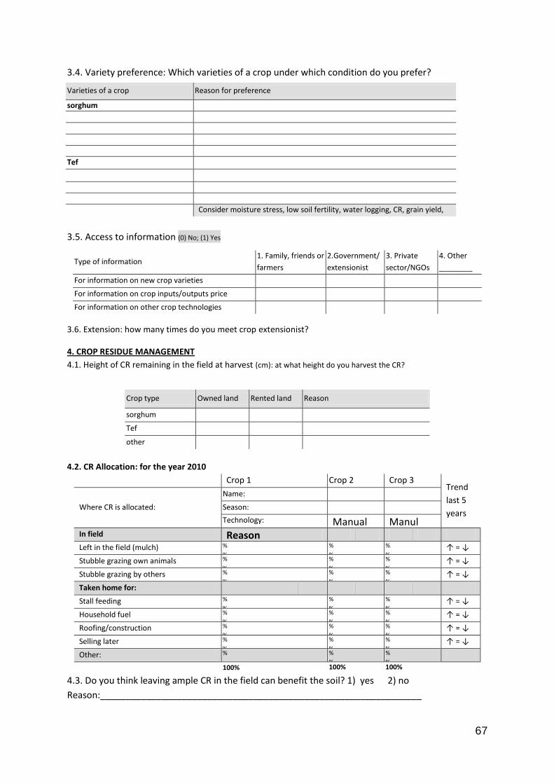
67
3.4. Variety preference: Which varieties of a crop under which condition do you prefer?
3.5. Access to information (0) No; (1) Yes
3.6. Extension: how many times do you meet crop extensionist?
4. CROP RESIDUE MANAGEMENT
4.1. Height of CR remaining in the field at harvest (cm): at what height do you harvest the CR?
4.2. CR Allocation: for the year 2010
Crop 1 Crop 2 Crop 3 Trend
last 5
years Where CR is allocated:
Name: Season: Technology:
Manual Manual Manul
In field Reason Left in the field (mulch) %
%
%
%
%
% ↑ = ↓
Stubble grazing own animals %
%
%
%
%
% ↑ = ↓
Stubble grazing by others %
%
%
%
%
% ↑ = ↓
Taken home for:
Stall feeding %
%
%
%
%
% ↑ = ↓
Household fuel %
%
%
%
%
% ↑ = ↓
Roofing/construction %
%
%
%
%
% ↑ = ↓
Selling later %
%
%
%
%
% ↑ = ↓
Other: %
%
%
%
%
100% 100% 100%
4.3. Do you think leaving ample CR in the field can benefit the soil? 1) yes 2) no
Reason:_______________________________________________________________
Varieties of a crop Reason for preference
sorghum
Tef
Consider moisture stress, low soil fertility, water logging, CR, grain yield,
etc
Type of information 1. Family, friends or
farmers
2.Government/
extensionist
3. Private
sector/NGOs
4. Other
________
For information on new crop varieties
For information on crop inputs/outputs price
For information on other crop technologies
Crop type Owned land Rented land Reason
sorghum
Tef
other
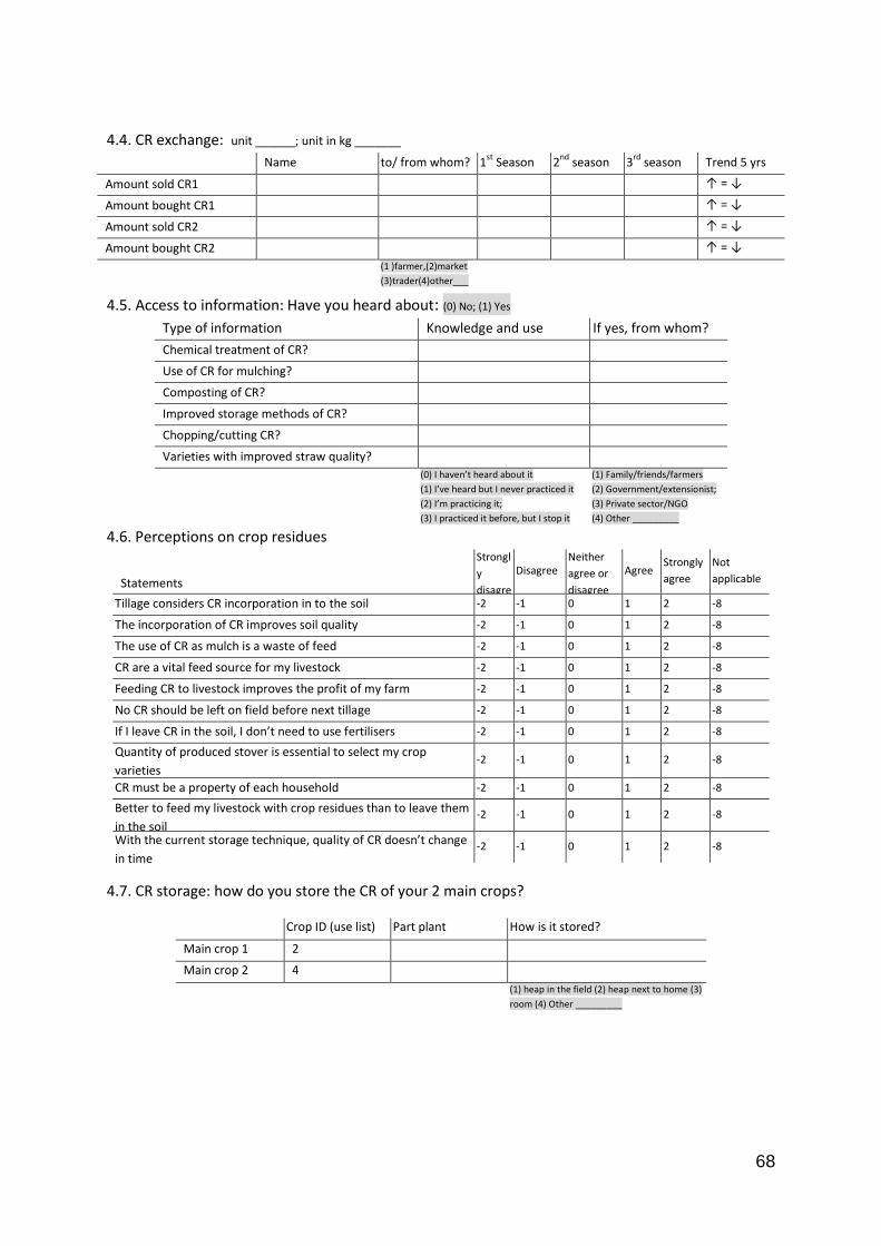
68
4.4. CR exchange: unit ______; unit in kg _______ Name to/ from whom? 1
st Season 2
nd season 3
rd season Trend 5 yrs
Amount sold CR1 ↑ = ↓
Amount bought CR1 ↑ = ↓
Amount sold CR2 ↑ = ↓
Amount bought CR2 ↑ = ↓
(1 )farmer,(2)market
(3)trader(4)other___
4.5. Access to information: Have you heard about: (0) No; (1) Yes
Type of information Knowledge and use If yes, from whom?
Chemical treatment of CR? Use of CR for mulching? Composting of CR? Improved storage methods of CR? Chopping/cutting CR? Varieties with improved straw quality?
(0) I haven’t heard about it
(1) I’ve heard but I never practiced it
(2) I’m practicing it;
(3) I practiced it before, but I stop it
(1) Family/friends/farmers
(2) Government/extensionist;
(3) Private sector/NGO
(4) Other _________
4.6. Perceptions on crop residues
Statements
Strongl
y
disagre
e
Disagree Neither
agree or
disagree
Agree Strongly
agree
Not
applicable
Tillage considers CR incorporation in to the soil -2 -1 0 1 2 -8
The incorporation of CR improves soil quality -2 -1 0 1 2 -8
The use of CR as mulch is a waste of feed -2 -1 0 1 2 -8
CR are a vital feed source for my livestock -2 -1 0 1 2 -8
Feeding CR to livestock improves the profit of my farm -2 -1 0 1 2 -8
No CR should be left on field before next tillage -2 -1 0 1 2 -8
If I leave CR in the soil, I don’t need to use fertilisers -2 -1 0 1 2 -8
Quantity of produced stover is essential to select my crop
varieties -2 -1 0 1 2 -8
CR must be a property of each household -2 -1 0 1 2 -8
Better to feed my livestock with crop residues than to leave them
in the soil -2 -1 0 1 2 -8
With the current storage technique, quality of CR doesn’t change
in time -2 -1 0 1 2 -8
4.7. CR storage: how do you store the CR of your 2 main crops?
Crop ID (use list) Part plant How is it stored?
Main crop 1 2
Main crop 2 4
(1) heap in the field (2) heap next to home (3)
room (4) Other _________
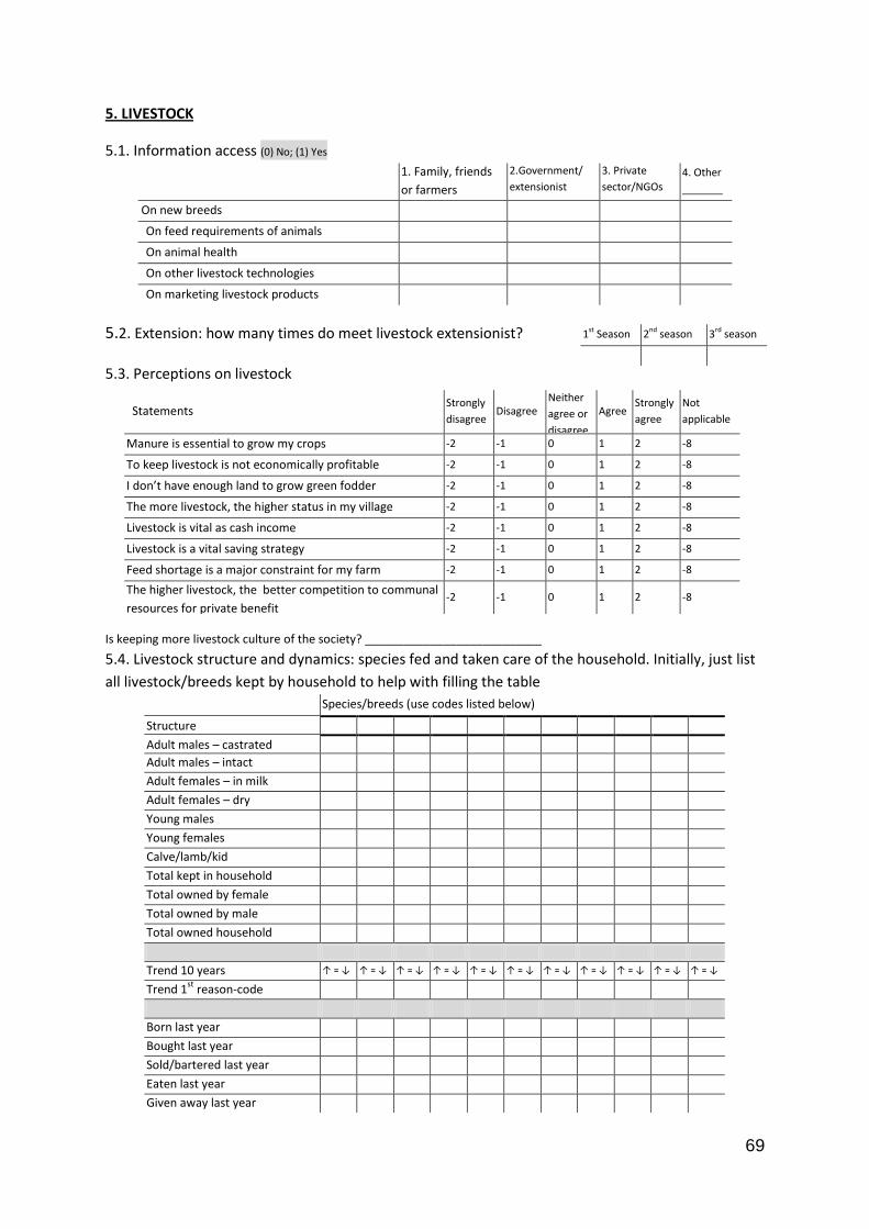
69
5. LIVESTOCK
5.1. Information access (0) No; (1) Yes
1. Family, friends
or farmers
2.Government/
extensionist
3. Private
sector/NGOs 4. Other
_______
On new breeds
On feed requirements of animals
On animal health
On other livestock technologies
On marketing livestock products
5.2. Extension: how many times do meet livestock extensionist?
5.3. Perceptions on livestock
Is keeping more livestock culture of the society? ___________________________
5.4. Livestock structure and dynamics: species fed and taken care of the household. Initially, just list
all livestock/breeds kept by household to help with filling the table
Species/breeds (use codes listed below)
Structure
Adult males – castrated
Adult males – intact
Adult females – in milk
Adult females – dry
Young males
Young females
Calve/lamb/kid
Total kept in household
Total owned by female
Total owned by male
Total owned household
Trend 10 years ↑ = ↓ ↑ = ↓ ↑ = ↓ ↑ = ↓ ↑ = ↓ ↑ = ↓ ↑ = ↓ ↑ = ↓ ↑ = ↓ ↑ = ↓ ↑ = ↓
Trend 1st
reason-code
Born last year
Bought last year
Sold/bartered last year
Eaten last year
Given away last year
1st Season 2nd season 3rd season
Statements Strongly
disagree Disagree
Neither
agree or
disagree
Agree Strongly
agree
Not
applicable
Manure is essential to grow my crops -2 -1 0 1 2 -8
To keep livestock is not economically profitable -2 -1 0 1 2 -8
I don’t have enough land to grow green fodder -2 -1 0 1 2 -8
The more livestock, the higher status in my village -2 -1 0 1 2 -8
Livestock is vital as cash income -2 -1 0 1 2 -8
Livestock is a vital saving strategy -2 -1 0 1 2 -8
Feed shortage is a major constraint for my farm -2 -1 0 1 2 -8
The higher livestock, the better competition to communal
resources for private benefit -2 -1 0 1 2 -8
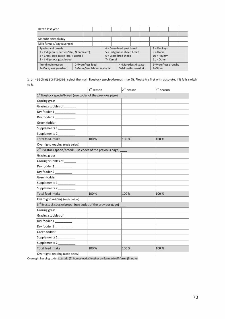
70
Death last year
Manure animal/day
Milk female/day (average)
Species and breeds 1 = Indigenous cattle (Zebu, N’dama etc) 2 = Cross-bred cattle (Ind. x Exotic ) 3 = Indigenous goat breed
4 = Cross-bred goat breed 5 = Indigenous sheep breed 6 = Cross-bred sheep 7= Camel
8 = Donkeys 9 = Horse 10 = Poultry 11 = Other
Trend main reason 1=More/less grassland
2=More/less feed 3=More/less labour available
4=More/less disease 5=More/less market
6=More/less drought 7=Other
5.5. Feeding strategies: select the main livestock species/breeds (max 3). Please try first with absolute, if it fails switch
to %.
1st
season 2nd
season 3rd
season
1st
livestock specie/breed (use codes of the previous page) ____
Grazing grass
Grazing stubbles of _______
Dry fodder 1 ____________
Dry fodder 2 ____________
Green fodder
Supplements 1 __________
Supplements 2 __________
Total feed intake 100 % 100 % 100 % Overnight keeping (code below)
2nd
livestock specie/breed: (use codes of the previous page) ____
Grazing grass
Grazing stubbles of _______
Dry fodder 1 __________
Dry fodder 2 __________
Green fodder
Supplements 1 __________
Supplements 2 __________
Total feed intake 100 % 100 % 100 % Overnight keeping (code below)
3rd
livestock specie/breed: (use codes of the previous page) ____
Grazing grass
Grazing stubbles of _______
Dry fodder 1 __________
Dry fodder 2 __________
Green fodder
Supplements 1 __________
Supplements 2 __________
Total feed intake 100 % 100 % 100 % Overnight keeping (code below)
Overnight keeping codes (1) stall; (2) homestead; (3) other on-farm; (4) off-farm; (5) other
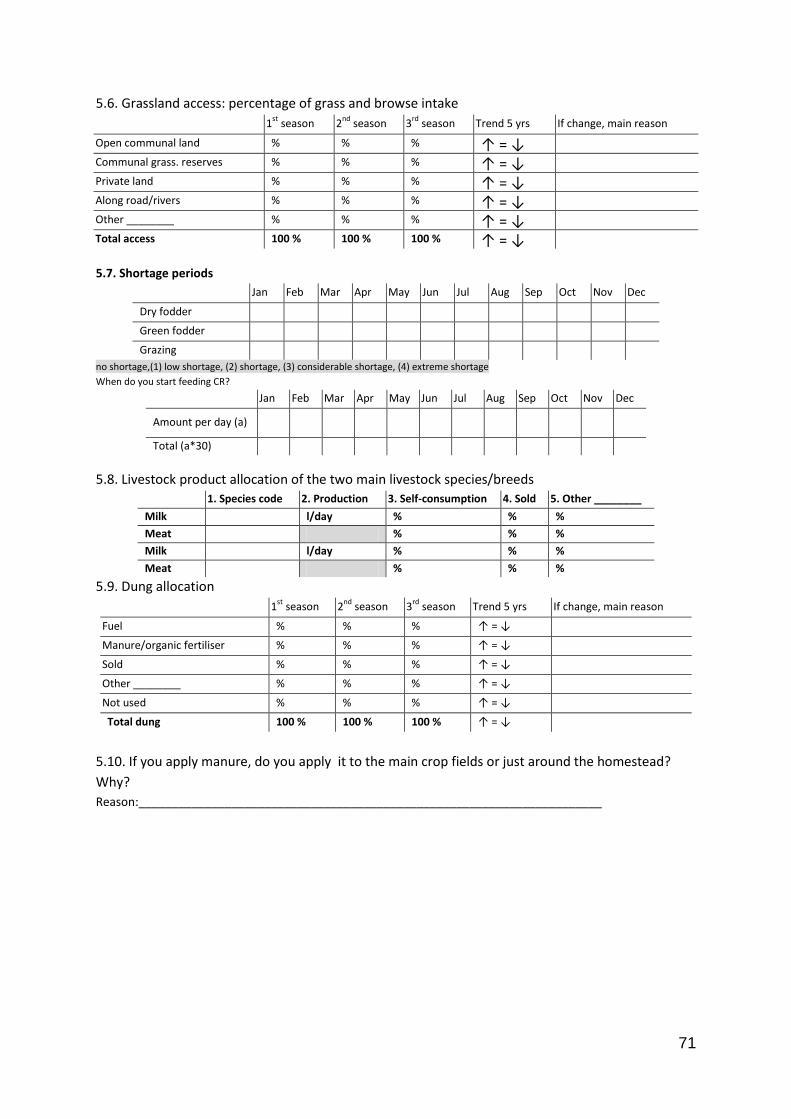
71
5.6. Grassland access: percentage of grass and browse intake
1st
season 2nd
season 3rd
season Trend 5 yrs If change, main reason
Open communal land % % % ↑ = ↓ Communal grass. reserves % % % ↑ = ↓ Private land % % % ↑ = ↓ Along road/rivers % % % ↑ = ↓ Other ________ % % % ↑ = ↓ Total access 100 % 100 % 100 % ↑ = ↓
5.7. Shortage periods
Jan Feb Mar Apr May Jun Jul Aug Sep Oct Nov Dec
Dry fodder
Green fodder
Grazing
no shortage,(1) low shortage, (2) shortage, (3) considerable shortage, (4) extreme shortage
When do you start feeding CR?
Jan Feb Mar Apr May Jun Jul Aug Sep Oct Nov Dec
Amount per day (a)
Total (a*30)
5.8. Livestock product allocation of the two main livestock species/breeds
1. Species code 2. Production 3. Self-consumption 4. Sold 5. Other ________
Milk l/day % % %
Meat % % %
Milk l/day % % %
Meat % % %
5.9. Dung allocation
1st
season 2nd
season 3rd
season Trend 5 yrs If change, main reason
Fuel % % % ↑ = ↓
Manure/organic fertiliser % % % ↑ = ↓
Sold % % % ↑ = ↓
Other ________ % % % ↑ = ↓
Not used % % % ↑ = ↓
Total dung 100 % 100 % 100 % ↑ = ↓
5.10. If you apply manure, do you apply it to the main crop fields or just around the homestead?
Why?
Reason:______________________________________________________________________
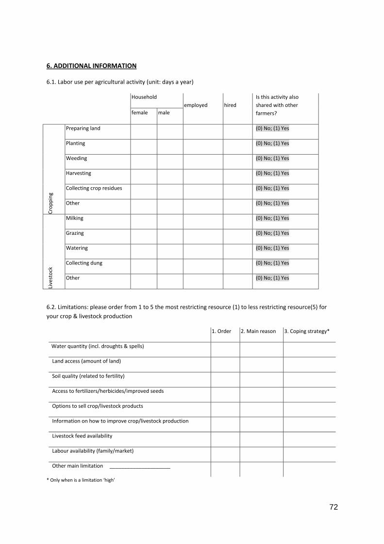
72
6. ADDITIONAL INFORMATION
6.1. Labor use per agricultural activity (unit: days a year)
Household
employed hired
Is this activity also
shared with other
farmers? female male
Cro
pp
ing
Preparing land (0) No; (1) Yes
Planting (0) No; (1) Yes
Weeding (0) No; (1) Yes
Harvesting (0) No; (1) Yes
Collecting crop residues (0) No; (1) Yes
Other (0) No; (1) Yes
Live
sto
ck
Milking (0) No; (1) Yes
Grazing (0) No; (1) Yes
Watering (0) No; (1) Yes
Collecting dung (0) No; (1) Yes
Other (0) No; (1) Yes
6.2. Limitations: please order from 1 to 5 the most restricting resource (1) to less restricting resource(5) for
your crop & livestock production
1. Order 2. Main reason 3. Coping strategy*
Water quantity (incl. droughts & spells)
Land access (amount of land)
Soil quality (related to fertility)
Access to fertilizers/herbicides/improved seeds
Options to sell crop/livestock products
Information on how to improve crop/livestock production
Livestock feed availability
Labour availability (family/market)
Other main limitation _____________________
* Only when is a limitation ‘high’
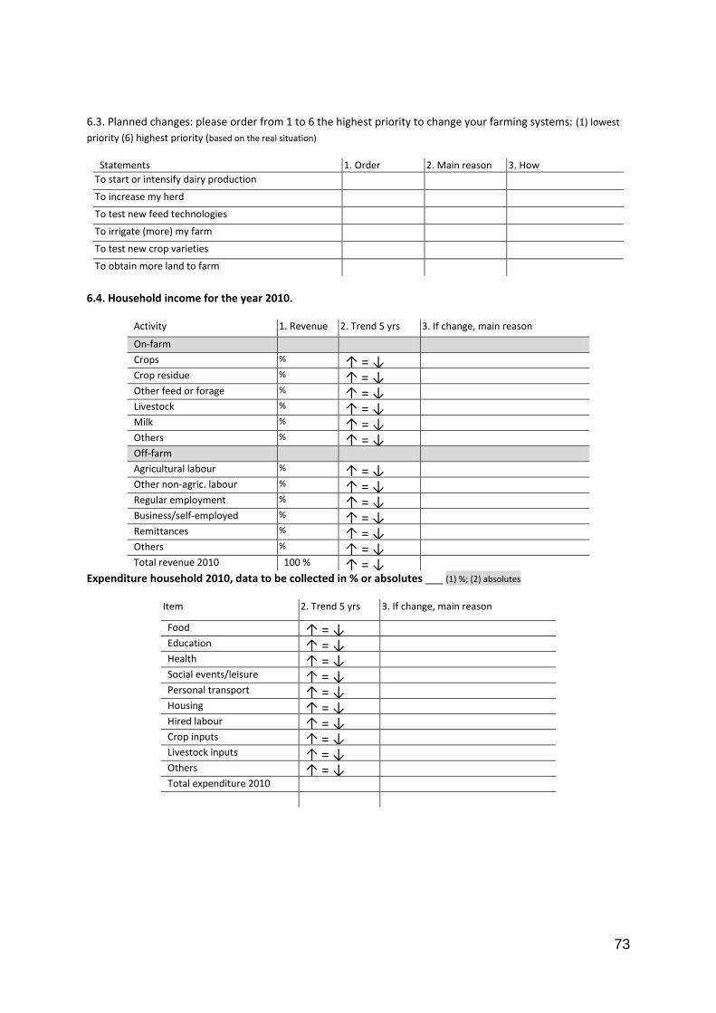
73
6.3. Planned changes: please order from 1 to 6 the highest priority to change your farming systems: (1) lowest
priority (6) highest priority (based on the real situation)
Statements 1. Order 2. Main reason 3. How
To start or intensify dairy production
To increase my herd
To test new feed technologies
To irrigate (more) my farm
To test new crop varieties
To obtain more land to farm
6.4. Household income for the year 2010.
Activity 1. Revenue 2. Trend 5 yrs 3. If change, main reason
On-farm
Crops % ↑ = ↓
Crop residue % ↑ = ↓
Other feed or forage % ↑ = ↓
Livestock % ↑ = ↓
Milk % ↑ = ↓
Others % ↑ = ↓
Off-farm
Agricultural labour % ↑ = ↓
Other non-agric. labour % ↑ = ↓
Regular employment % ↑ = ↓
Business/self-employed % ↑ = ↓
Remittances % ↑ = ↓
Others % ↑ = ↓
Total revenue 2010 100 % ↑ = ↓
Expenditure household 2010, data to be collected in % or absolutes ___ (1) %; (2) absolutes
Item 2. Trend 5 yrs 3. If change, main reason
Food ↑ = ↓
Education ↑ = ↓
Health ↑ = ↓
Social events/leisure ↑ = ↓
Personal transport ↑ = ↓
Housing ↑ = ↓
Hired labour ↑ = ↓
Crop inputs ↑ = ↓
Livestock inputs ↑ = ↓
Others ↑ = ↓
Total expenditure 2010
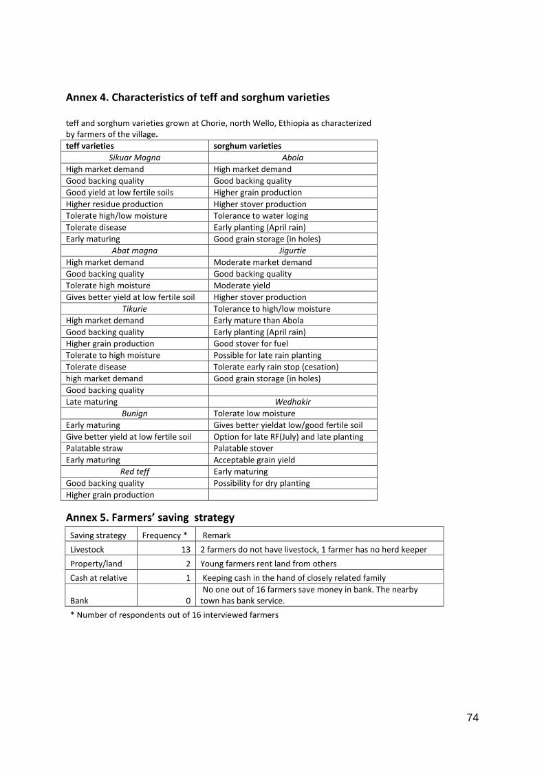
74
Annex 4. Characteristics of teff and sorghum varieties
teff and sorghum varieties grown at Chorie, north Wello, Ethiopia as characterized by farmers of the village.
teff varieties sorghum varieties
Sikuar Magna Abola
High market demand High market demand
Good backing quality Good backing quality
Good yield at low fertile soils Higher grain production
Higher residue production Higher stover production
Tolerate high/low moisture Tolerance to water loging
Tolerate disease Early planting (April rain)
Early maturing Good grain storage (in holes)
Abat magna Jigurtie
High market demand Moderate market demand
Good backing quality Good backing quality
Tolerate high moisture Moderate yield
Gives better yield at low fertile soil Higher stover production
Tikurie Tolerance to high/low moisture
High market demand Early mature than Abola
Good backing quality Early planting (April rain)
Higher grain production Good stover for fuel
Tolerate to high moisture Possible for late rain planting
Tolerate disease Tolerate early rain stop (cesation)
high market demand Good grain storage (in holes)
Good backing quality
Late maturing Wedhakir
Bunign Tolerate low moisture
Early maturing Gives better yieldat low/good fertile soil
Give better yield at low fertile soil Option for late RF(July) and late planting
Palatable straw Palatable stover
Early maturing Acceptable grain yield
Red teff Early maturing
Good backing quality Possibility for dry planting
Higher grain production
Annex 5. Farmers’ saving strategy
Saving strategy Frequency * Remark
Livestock 13 2 farmers do not have livestock, 1 farmer has no herd keeper
Property/land 2 Young farmers rent land from others
Cash at relative 1 Keeping cash in the hand of closely related family
Bank 0 No one out of 16 farmers save money in bank. The nearby town has bank service.
* Number of respondents out of 16 interviewed farmers
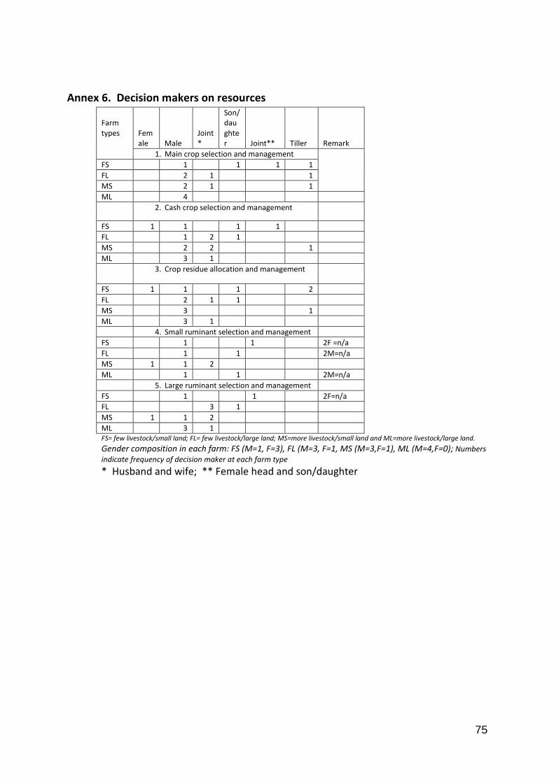
75
Annex 6. Decision makers on resources Farm types Fem
ale Male Joint*
Son/daughter Joint** Tiller Remark
1. Main crop selection and management
FS 1 1 1 1
FL 2 1 1
MS 2 1 1
ML 4
2. Cash crop selection and management
FS 1 1 1 1
FL 1 2 1
MS 2 2 1
ML 3 1
3. Crop residue allocation and management
FS 1 1 1 2
FL 2 1 1
MS 3 1
ML 3 1
4. Small ruminant selection and management
FS 1 1 2F =n/a
FL 1 1 2M=n/a
MS 1 1 2
ML 1 1 2M=n/a
5. Large ruminant selection and management
FS 1 1 2F=n/a
FL 3 1
MS 1 1 2
ML 3 1 FS= few livestock/small land; FL= few livestock/large land; MS=more livestock/small land and ML=more livestock/large land.
Gender composition in each farm: FS (M=1, F=3), FL (M=3, F=1, MS (M=3,F=1), ML (M=4,F=0); Numbers
indicate frequency of decision maker at each farm type
* Husband and wife; ** Female head and son/daughter
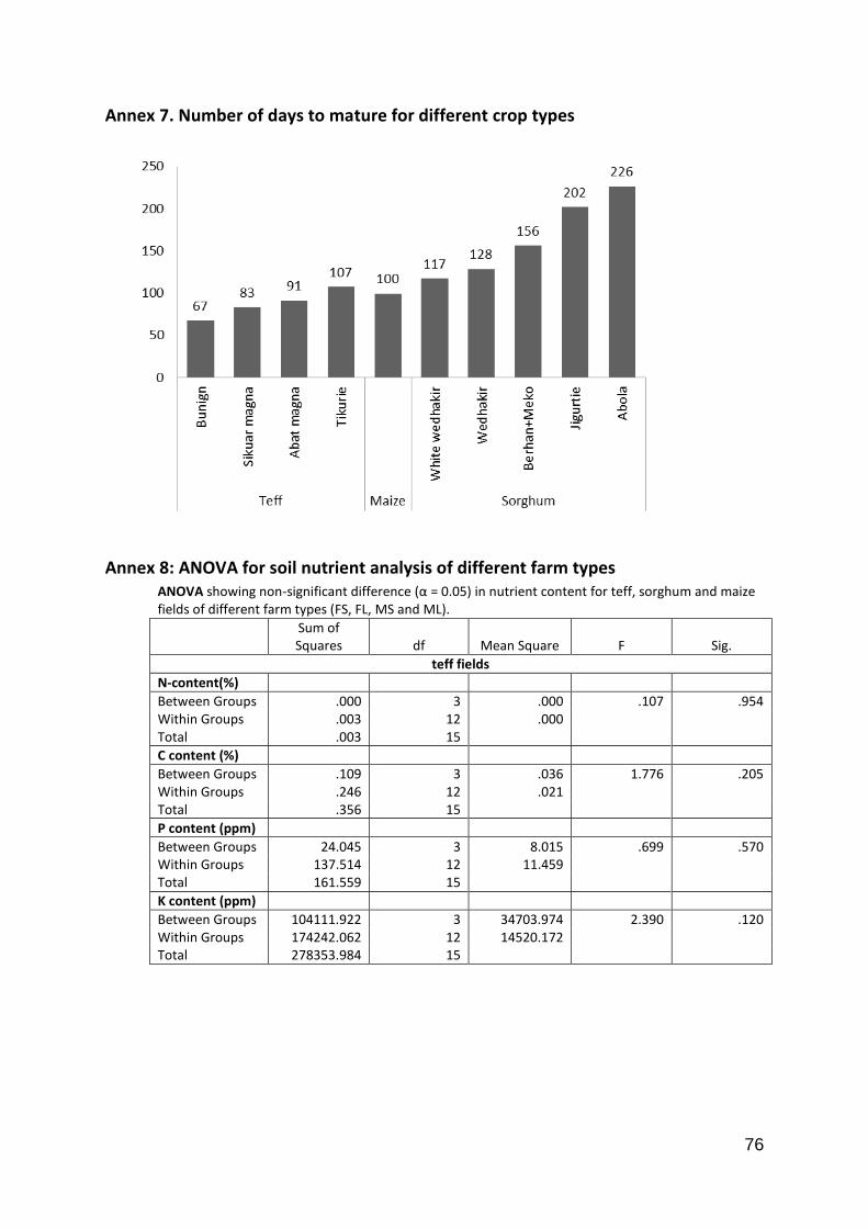
76
Annex 7. Number of days to mature for different crop types
Annex 8: ANOVA for soil nutrient analysis of different farm types ANOVA showing non-significant difference (α = 0.05) in nutrient content for teff, sorghum and maize fields of different farm types (FS, FL, MS and ML).
Sum of Squares df Mean Square F Sig.
teff fields
N-content(%)
Between Groups .000 3 .000 .107 .954 Within Groups .003 12 .000 Total .003 15
C content (%)
Between Groups .109 3 .036 1.776 .205 Within Groups .246 12 .021 Total .356 15
P content (ppm)
Between Groups 24.045 3 8.015 .699 .570 Within Groups 137.514 12 11.459 Total 161.559 15
K content (ppm)
Between Groups 104111.922 3 34703.974 2.390 .120 Within Groups 174242.062 12 14520.172 Total 278353.984 15
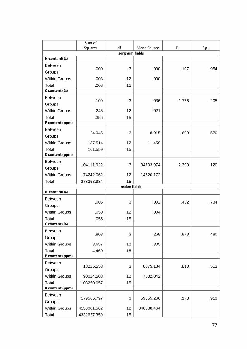
77
Sum of Squares df Mean Square F Sig.
sorghum fields
N-content(%)
Between
Groups .000 3 .000 .107 .954
Within Groups .003 12 .000
Total .003 15
C content (%)
Between
Groups .109 3 .036 1.776 .205
Within Groups .246 12 .021
Total .356 15
P content (ppm)
Between
Groups 24.045 3 8.015 .699 .570
Within Groups 137.514 12 11.459
Total 161.559 15
K content (ppm)
Between
Groups 104111.922 3 34703.974 2.390 .120
Within Groups 174242.062 12 14520.172
Total 278353.984 15
maize fields
N-content(%)
Between
Groups .005 3 .002 .432 .734
Within Groups .050 12 .004
Total .055 15
C content (%)
Between
Groups .803 3 .268 .878 .480
Within Groups 3.657 12 .305
Total 4.460 15
P content (ppm)
Between
Groups 18225.553 3 6075.184 .810 .513
Within Groups 90024.503 12 7502.042
Total 108250.057 15
K content (ppm)
Between
Groups 179565.797 3 59855.266 .173 .913
Within Groups 4153061.562 12 346088.464
Total 4332627.359 15

78