Embed Size (px)
Citation preview
Growth and Activity Diversification: the impact of financing non-traditional local activities
Thiago Christiano Silva and Benjamin Miranda Tabak
August 2019
498

ISSN 1518-3548 CGC 00.038.166/0001-05
Working Paper Series Brasília n. 498 August 2019 p. 1-64

Working Paper Series
Edited by Research Department (Depep) – E-mail: [email protected]
Editor: Francisco Marcos Rodrigues Figueiredo – E-mail: [email protected]
Co-editor: José Valentim Machado Vicente – E-mail: [email protected]
Head of Research Department: André Minella – E-mail: [email protected]
The Banco Central do Brasil Working Papers are all evaluated in double blind referee process.
Reproduction is permitted only if source is stated as follows: Working Paper n. 498.
Authorized by Carlos Viana de Carvalho, Deputy Governor for Economic Policy.
General Control of Publications
Banco Central do Brasil
Comun/Divip
SBS – Quadra 3 – Bloco B – Edifício-Sede – 2º subsolo
Caixa Postal 8.670
70074-900 Brasília – DF – Brazil
Phones: +55 (61) 3414-3710 and 3414-3565
Fax: +55 (61) 3414-1898
E-mail: [email protected]
The views expressed in this work are those of the authors and do not necessarily reflect those of the Banco Central or
its members.
Although these Working Papers often represent preliminary work, citation of source is required when used or reproduced.
As opiniões expressas neste trabalho são exclusivamente do(s) autor(es) e não refletem, necessariamente, a visão do Banco
Central do Brasil.
Ainda que este artigo represente trabalho preliminar, é requerida a citação da fonte, mesmo quando reproduzido parcialmente.
Citizen Service Division
Banco Central do Brasil
Deati/Diate
SBS – Quadra 3 – Bloco B – Edifício-Sede – 2º subsolo
70074-900 Brasília – DF – Brazil
Toll Free: 0800 9792345
Fax: +55 (61) 3414-2553
Internet: http//www.bcb.gov.br/?CONTACTUS
Non-Technical Summary
We study how financing non-traditional local activities, conceived here as a proxy for localactivity diversification, associates with economic growth. We use municipality-level datafrom Brazil, a country that provides an ideal experimental setup due to the large geographical,social, and economic disparities observed across its more than 5,500 cities.
Municipalities specialize in agricultural, industrial or service activities. We assume that thetraditional activity of a municipality is the one that contributes the most to its local GDP.The remainder sectors—those contributing less to the local GDP—are considered as non-traditional. Our proxy for finance to non-traditional local activities computes the share ofbank credit that is channeled to non-traditional sectors.
According to David Ricardo’s theory, countries should specialize in activities in which theyenjoy comparative advantage. From a cities viewpoint, if cities have different specializations—precisely their traditional local activities—then funding less important non-traditional sectorscould reduce their potential for development, which could otherwise be reached in case fund-ing were channeled to those activities with comparative advantage. In line with this theory, weshould expect a negative association between funding non-traditional local activities—whichcould promote activity diversification (less specialization)—and economic growth.
Using Brazilian data, our empirical exercises point to the opposite: funding non-traditionallocal activities associates with higher economic growth rates. Our finding can be relatedto several factors. First, non-traditional local sectors may be more profitable and thereforetheir funding is beneficial to growth. This could be due to a less competitive environmentor because some sectors experience decreasing returns of scale. Second, we could argue thatpromoting activity diversification can lead to a synergistic effect of these new activities andthe traditional local activity, making the city more attractive to new firms and households.
We show that funding non-traditional local activities associates with higher growth only inmoments of normality. We use natural disasters to test how financial development and fi-nancing non-traditional activities associate with economic growth in times of distress. Inadverse scenarios, we show that funding non-traditional local activities correlates negativelywith growth. That is, the focus on leveraging the comparative advantages seems to be morerelevant to achieve greater growth in times of distress.
3

Sumario Nao Tecnico
O trabalho investiga como o financiamento a atividades locais nao tradicionais nas cidades,concebidas aqui como uma proxy para a diversificacao de atividades locais, associa-se aocrescimento economico. Usam-se dados em nıvel municipal do Brasil, um paıs que forneceuma configuracao experimental ideal devido as grandes disparidades geograficas, sociais eeconomicas observadas em suas mais de 5.500 cidades.
Municıpios especializam-se em atividades agrıcolas, industriais ou de servicos. Assume-seque a atividade tradicional de um municıpio e aquela que mais contribui para o seu PIB. Ossetores restantes—aqueles que contribuem menos para o PIB local—sao considerados naotradicionais. A proxy para financiamento de atividades locais nao tradicionais e dada pelaparcela de credito bancario que e canalizada para setores nao tradicionais relativamente atodo credito bancario no municıpio.
Segundo a teoria de David Ricardo, os paıses deveriam se especializar em atividades nasquais eles desfrutam de vantagem comparativa. Do ponto de vista das cidades, se as cidadestiverem especializacoes diferentes—precisamente suas atividades locais tradicionais—, entaofinanciar setores nao tradicionais menos importantes poderia reduzir seu potencial de desen-volvimento, que poderia ser alcancado caso o financiamento bancario fosse canalizado paraaquelas atividades com vantagem comparativa. De acordo com essa teoria, deveria-se esperaruma associacao negativa entre o financiamento de atividades locais nao tradicionais—que pro-movem a diversificacao de atividades (menor especializacao)—e o crescimento economico.
Usando dados brasileiros, nossos exercıcios empıricos apontam para o oposto: o financia-mento de atividades locais nao tradicionais esta associado a taxas de crescimento economicomais altas. Este resultado pode estar relacionado a varios fatores. Primeiro, setores locaisnao tradicionais podem ser mais lucrativos e, portanto, seu financiamento e benefico para ocrescimento. Isso pode ser devido a existencia de um ambiente menos competitivo ou porquealguns setores possuem retornos decrescentes de escala. Segundo, poderia-se argumentar quea promocao da diversificacao de atividades leva a um efeito sinergico delas com a atividadelocal tradicional, tornando a cidade mais atraente para novas empresas e famılias.
Mostra-se tambem que o financiamento de atividades locais nao tradicionais associa-se a ummaior crescimento apenas em momentos de normalidade. Usando desastres naturais, testa-secomo desenvolvimento financeiro e o financiamento a atividades nao tradicionais se associamcom crescimento economico em tempos de estresse. Durante cenarios adversos, financiaratividades locais nao tradicionais se correlaciona de forma negativa com crescimento. Ouseja, o foco em alavancar as vantagens comparativas parece ser mais relevante para alcancarum maior crescimento em tempos de estresse.
4
Growth and Activity Diversification:the impact of financing non-traditional local activities
Thiago Christiano Silva*
Benjamin Miranda Tabak**
AbstractWe study how financing non-traditional local activities, conceived here as a proxy for activity diver-sification, associates with economic growth. We use municipality-level data from Brazil, a countrythat provides an ideal experimental setup due to the large geographical, social, and economic dis-parities observed across its more than 5,500 cities. We find that financing non-traditional localactivities matters to cities development and such association is stronger at their earlier stages of de-velopment. We use the centrality in the network of intercity economic flows as a proxy for the mu-nicipality stage of development. The centrality encodes the overall importance of the city in termsof economic intermediation to the entire network structure of business activities. The network isconstructed using every observed intercity wire transfers registered in the Brazilian Payments Sys-tem. Cities more nearby (geographic closeness) and that transact more (economic closeness) withadvanced centers have higher growth rates, suggesting the existence of positive spillovers. Eco-nomic spillovers are more critical than geographic spillovers for growth. Using natural disastersas sources of unexpected negative events, we also find that the inverted U-shaped association offinancial development variables with growth commonly documented in the finance-growth liter-ature breaks down. In addition, the association between financing non-traditional local activitiesand economic growth becomes negative in times of distress. Our results suggest that cities shouldrestrengthen their traditional activities when adverse conditions befall.
Keywords: activity diversification, finance-growth nexus, spillovers, financial intermediation, tradenetworks, payments networks.JEL Classification: O47, G32, G21, F15, F18, C10.
The Working Papers should not be reported as representing the views of the Banco Central doBrasil. The views expressed in the papers are those of the authors and do not necessarily reflectthose of the Banco Central do Brasil.
*Research Department, Banco Central do Brasil, e-mail: [email protected].**FGV/EPPG Escola de Polıticas Publicas e Governo, Fundacao Getulio Vargas (School of Public Policy and Govern-
ment, Getulio Vargas Foundation), e-mail: [email protected].
5
1 Introduction
In a seminal paper, King and Levine (1993) show that financial development positively impacts eco-nomic growth using a cross-country study.1 A new strand of the finance-growth literature argues thatsuch relationship lasts up to a point, above which the marginal benefits of financial development oneconomic growth start to decrease and can even become predatory.2
The finance-growth literature constructs proxies for financial development at the aggregate level whenexplaining local economic growth. Some few exceptions study the relationship between growth andfinancial development using bank credit operations from the creditor perspective.3 In contrast, thispaper looks at the borrower side of the credit relationship. We analyze how borrowers’ activities relateto the city traditional and non-traditional activities and whether they impact local economic growth indifferent ways. Thus, this paper documents the role of lending diversification in economic growth.
We show that the distribution of who gets the credit (borrowers) matters for economic growth. Accord-ing to David Ricardo’s theory, countries should specialize in activities in which they enjoy comparativeadvantage. From a cities viewpoint, if cities have different specializations—precisely their traditionallocal activities—then funding less important non-traditional sectors could reduce their potential for de-velopment, which would otherwise be reached in case funding were channeled to those activities withcomparative advantage.
Therefore, according to the Ricardian theory, we should expect a negative association between fundingnon-traditional local activities—which could promote activity diversification (less specialization)—and economic growth. Using a rich data set with all municipalities in Brazil, we show the opposite:funding non-traditional local activities associates with higher economic growth rates.4
Our finding can be related to several factors. First, non-traditional local sectors may be more profitableand therefore their funding is beneficial to growth. This could be due to a less competitive environmentor because some sectors experience decreasing returns of scale.5 Second, we could argue that promot-
1Since then, the literature has provided several empirical findings that corroborate this positive relationship. For in-stance, Jayaratne and Strahan (1996) document that financial markets can directly affect economic growth by studying therelaxation of bank branch restrictions in the United States. See also Levine and Zervos (1998), Rajan and Zingales (1998),Beck et al. (2000), Beck and Levine (2004), Levine (2005), Soedarmono et al. (2017), Beck et al. (2014a), and Beck et al.(2015).
2Law and Singh (2014), Rioja and Valev (2004), Samargandi et al. (2015), Soedarmono et al. (2017), and Abedifaret al. (2016) explore this non-linear dependency.
3For example, Abedifar et al. (2016) and Andersson et al. (2016) evaluate the contribution of public or private banks tolocal economic growth.
4We take Brazil as a case study due to several reasons. First, Brazil is a relevant emerging market country that ex-perienced a tremendous credit growth in the mid-2000s. Despite such strong credit growth, the pace of economic growthhas been somewhat lower and therefore the link between bank credit and growth is important to be explored. Second, thestructure of the economy is also bank-oriented. In this way, bank credit ends up being the only source of external fundingfor the average firm. Therefore, the study of the relevance of banks to economic growth of Brazilian cities is amplified.Third, Brazil has a large geographical territory with significant demographic, social and economic disparities observedacross its more than 5,500 existent cities. This setup provides a large cross-sectional and temporal heterogeneity to checkour empirical hypotheses.
5Imagine a city specialized in agriculture and industrial activities, but with no services facilities. The introduction ofa services facilities could make a bigger difference than the introduction of a new factory or a new farm. In the former,returns are much higher due to the low actual levels of services provided by the city.
6
ing activity diversification can lead to a synergistic effect of these new activities and the traditionallocal activity.6
We use natural disasters as sources of exogenous distress to measure whether the positive associationbetween activity diversification and economic growth still holds in times of distress. In these adversescenarios, we show that the correlation between funding non-traditional local activities and growthbecomes negative. That is, the focus on leveraging—or even restoring—the comparative advantagesseems to be more relevant to achieve greater growth in times of distress.
Economic growth not only depends on local characteristics of cities, but also on other city counterpartsto which they connect. Interconnections between two cities can arise due to geographical proximityand also to economic relationships, regardless of distances. While we find that the existence of bothtypes of interconnections correlates with higher economic growth—suggesting the existence of positivespillovers due to city integration—economic relationships associate with growth more strongly thangeographical proximity. This effect may be due to the large dimensions of Brazil and to the greatdistances between cities.
These results are relevant for thinking about the development of public policies seeking to create con-ditions for different regions of the country to develop. Infrastructure investments that allow citiesto increase trade flows between them should have positive effects on the cities benefiting from theseinvestments.
To the best of our knowledge, this is the first paper that shows evidence that trade connections andgeography matter for the relationship between financial development and economic growth, as well asdocumenting their relative importance to growth. Our results open a new avenue for further researchon the effect of distinct public policies on economic growth, and on the relationship between financialdevelopment and economic growth for other countries.
Municipalities specialize in agricultural, industrial or service activities. We assume that the traditionalactivity of a municipality is the one that contributes the most to its local GDP. The remainder sectors—those contributing less to the local GDP—are considered as non-traditional.7 Our proxy for finance tonon-traditional local activities computes the share of bank credit that is channeled to non-traditionalsectors.
We use loan-level data from the Brazilian Credit Risk Register (SCR) to identify how banks channelcredit to firms within cities. We then merge this loan-level data set with city-level data from theBrazilian Institute of Geography and Statistics (IBGE) and with firm-level data from the BrazilianInternal Revenue Service (IRS) to classify borrower’s activity as traditional or non-traditional within
6For instance, cities become more attractive to households and even firms when they have all services and facilities atdisposal of their residents.
7As cities develop, they naturally become complex and start performing several activities, potentially complementary toeach other. As a result, they may have more than a single traditional activity. For instance, Sao Paulo is the largest Braziliancity with similar total added values in the industry and services sectors. In this way, there is an ambiguity in defining thetraditional activity of such cities. In fact, the most complex and developed cities in Brazil often have this duality withrespect to their traditional activities. In unreported results, we also run regressions considering as the non-traditional localactivity the one that contributes the least to the local GDP, instead of all the sectors other than the one that contributes themost (baseline regressions shown in this paper). Results remain qualitatively the same.
7
the boundaries of the city where it resides. Therefore, we can track traditional and non-traditionalactivities in each municipality and evaluate how much bank financing each activity receives over time.We find a substantial heterogeneity of business specializations and degrees of finance to non-traditionallocal activities across Brazilian municipalities.
We find evidence that cities at advanced stages of development—higher network centrality—correlatewith higher rates of economic growth. We compute the city centrality using the network of intercitywire transfers built from more than 410 million business-oriented, firm-to-firm transfers in Brazil.8
We find the positive association between finance to non-traditional local activities and growth weakensas cities become more economically developed. In these municipalities, firms have other forms offunding, such as retained earnings, capital or corporate markets, and therefore rely less on bank lending.In this case, bank credit becomes ancillary to the local economy of advanced municipalities.
The paper proceeds as follows. Section 2 discusses the related literature. Section 3 presents the data.Section 4 introduces the variables and discusses the econometric methodology. Section 5 discusses theempirical results. Section 6 concludes the paper.
2 Related Literature
Our work connects to existing researches by reinforcing the classical link between financial develop-ment and economic growth (King and Levine (1993), Levine and Zervos (1998), Rajan and Zingales(1998), Beck et al. (2000), Beck and Levine (2004), Levine (2005), Soedarmono et al. (2017), Becket al. (2014a), and Beck et al. (2015)). In line with the literature, we document a positive associa-tion between financial development—proxied by deposits, credit, and financial system size—and localeconomic growth rates using municipality-level data from Brazil. Our work also reports that such mu-tualistic relationship lasts up to a point, above which it weakens and can eventually become negative.Such non-linearity and the existence of this critical point in the finance-growth nexus reinforce empir-ical evidence reported in more recent finance-growth papers using cross-country data (Law and Singh(2014), Rioja and Valev (2004), Samargandi et al. (2015), Soedarmono et al. (2017), and Abedifar et al.(2016)).
The non-linearity in the finance-growth relationship may arise for several reasons. The financial systemmay compete with the real sector for resources and may attract talented people that would be otherwiseworking in the real sector. Therefore, with lower levels of human capital, the real sector would havelower productivity and growth as a consequence (Tobin (1984)).
8The intercity trade network is a large-scale, weighted digraph. The weights are the payments and the link orientationarises from the payment flow nature (payer and receiver). By aggregating firm-to-firm to city-to-city transfers, we computethe network centrality of each municipality with the aid of the complex network theory (Silva et al. (2016a,b), Rossi et al.(2018), and El-Khatib et al. (2015)). We use the Google PageRank centrality, which is a feedback-based network measurethat depends on two components: the degree and the quality of interconnectivity. While the degree of interconnectivityrelates to the number of transactions that municipalities perform with other cities, the quality of interconnectivity pertainsto the relative importance of the peers with which cities transact. Higher centrality for a city means that it transacts a lot(degree) and with outstanding (quality) municipalities.
8
As the financial sector develops, several financial intermediaries may incur in excessive leverage, whichmay induce more significant economic fluctuations with an adverse effect on economic growth (Rajan(2006)). The incentive to take excessive risks in more developed financial systems is one of the poten-tial channels that may explain a non-linear relationship between finance and growth, dampening theeffect of financial development on growth after a certain threshold.
The development of the financial sector may increase the number of non-intermediation activities andtheir relevance to financial intermediaries. These non-traditional activities may have a smaller effecton economic growth than the traditional financial intermediation activity. Therefore, with the increasein the development of the financial sector, there may be a threshold from which financial developmenthas little or a negative effect on economic growth (Beck et al. (2014b)).
It is important to stress that most studies that relate financial development to economic growth usea cross-country sample (Rousseau and Wachtel (2002), Slesman et al. (2019) Morganti and Garofalo(2019), Herwartz and Walle (2014), and Law et al. (2013)). There are substantial differences amongcountries, suggesting that we have to evaluate the results of these studies carefully. It is difficult tocontrol for all possible distinctions among countries, such as differences in the legal framework, qualityof institutions, levels of human development, corruption, among many others. Our focused study ona single country with more granular data is useful to avoid eventual omitted variable biases that arelikely to appear in cross-country studies. Municipalities in Brazil are roughly subject to the same legalconstraints all over the country, which minimizes omitted variable issues. Such microdata also allowsstudying the relevance of the geographical distribution of financial development on economic growthwithin a country (Kendall (2012)).
The Ricardian theory on comparative advantage has some support from empirical research. It is es-tablished by now that if a country specializes in specific products or services using its comparativeadvantages, then it will have trade gains with other countries. Konstantakopoulou and Tsionas (2019)show that for the Euro area comparative advantages positively affect export specialization.9 However,the case of Brazil is that of a continental country with a large variety of comparative advantages. Inthis case, there may be gains from economic diversification. This is most true when they have comple-mentary effects that help foster production in the main traditional sector. For example, Freire (2019)shows empirical evidence that economic diversification is essential for developing countries in orderto create jobs and foster economic development.
3 Data Description
In this paper, we put together and match supervisory and public data from several sources. We analyzethe period from 2003 to 2014 in Brazil.10 This section reports how we construct, collect, and pre-
9They find reverse causality for several countries as well.10On the one hand, we cannot move the lower bound date limit because of unavailability of credit data. On the other
hand, we cannot move further the upper bound date limit because of the absence of municipality-level data on growth andtraditional business activity. Data on natural disasters and intercity and intracity payment flows do not bind the limits of theanalyzed period in neither directions.
9
process each variable used in the empirical part of the paper.
According to the IBGE, Brazil had 5,570 municipalities in 2014. In light of its vast territorial exten-sion, Brazil has five central regions: North (550 municipalities), Northeast (1,794), Midwest (467),Southeast (1,668), and South (1,191). The number of Brazilian municipalities grows until 2010, afterwhich it stagnates. Such dynamics is explained by the fact that the creation of new municipalities hadto comply with more stringent regulation after 2010, leading to a reduction of new municipalities.11
We use the SCR to keep track of ongoing credit operations of firms in Brazil.12 Information is con-fidential and comes from the Banco Central do Brasil (BCB). The data set includes the bank andclient identification (tax identifier); loan-level characteristics, such as time to maturity, overdue parcels,modality, the origin of the credit (earmarked and non-earmarked), interest rate, risk classification; andcollateral information. We use this dataset to identify the bank credit volume across municipalities inBrazil.
There are over 24 million outstanding bank credit operations channeled to firms from 2003 to 2014.We consider credit operations granted from all commercial (159 banks), investment (72), developmentbanks (5) and also credit unions (1,235) operating in Brazil. The banking sector comprises state-owned banks—which hold a substantial share of the business loans market—domestic private, andalso foreign private banks. Our sample includes business (profit-oriented) and non-profit firms, whichexert activities in the agriculture, industry, and/or services sectors.13 We have over 6.2 million firmheadquarters in our sample.
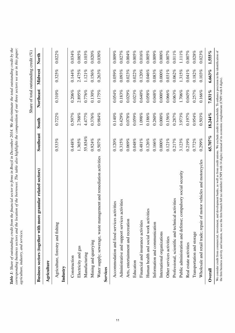
Table 1 reports the share of the total outstanding bank credit to firms in Brazil during 2014 broken downby the borrower’s location and business activity. Bank credit goes predominantly to the Southeast andSouth regions, which have the highest levels of development in Brazil. For example, the Southeastregion accounts for 65.71% of the total outstanding bank credit of the country in 2014. Less devel-oped regions, such as the North and Midwest, are responsible for only 8.22% in 2014. The relativeimportance of Brazilian regions remains stable over time.
In the Southeast region, firms in the manufacturing business sector respond with more than 50% of alloutstanding bank credit in 2014, fact that evidences the massive industrialization in the region. Creditin the South region has a higher dispersion across different sectors. Though manufacturing firms also
11The constitutional amendment (CA) 15 in 2006 made more rigorous the creation of new municipalities. Despite that,many municipalities were created after that mainly due to financial benefits that municipalities enjoy from compulsoryfederal government transfers guaranteed by the Federal Constitution. The establishment of new municipalities did not stopeven with the publication of the CA 15/2006 because such law was not auto-executory: it required further legislation to belegally enforceable. In 2008, another CA came into force and validated those municipalities created after 2006 to put anend to the uncertainty revolving around their legal status. The creation of municipalities after 2010 is facing considerablelegal uncertainty, which has been preventing the constitution of new cities. One of the main recent requirements is thatparties involved in the municipality creation have to show the economic viability of the act and the population needs to voteand confirm its creation.
12SCR is a comprehensive data set which records every single credit operation within the Brazilian financial systemworth R$200 or above. Up to June 30th, 2016, this lower limit was R$1,000. Therefore, most of the data we are assessingfollows this rule.
13We exclude credit to the public administration and extraterritorial entities with branches located in Brazil, such asforeign diplomatic representations. In this way, we focus on credit to business firms and how it affects local growth. Wefollow the same arguments when matching and filtering other datasets.
10
T abl
e1:
Shar
eof
outs
tand
ing
cred
itfr
omth
efin
anci
alse
ctor
tofir
ms
inB
razi
lin
Dec
embe
r20
14.W
edi
scri
min
ate
the
tota
lout
stan
ding
cred
itby
the
corr
espo
ndin
gbu
sine
ssse
ctor
san
dth
elo
catio
nof
the
borr
ower
.Th
eta
ble
also
high
light
sth
eco
mpo
sitio
nof
our
thre
ese
ctor
sw
eus
ein
this
pape
r:ag
ricu
lture
,ind
ustr
y,an
dse
rvic
es.
Shar
eof
tota
lout
stan
ding
cred
it(%
)
Bus
ines
s sec
tors
(tog
ethe
rw
ithm
ore
gran
ular
rela
ted
sect
ors)
Sout
heas
tSo
uth
Nor
thea
stM
idw
est
Nor
th
Agr
icul
ture
Agr
icul
ture
,for
estr
yan
dfis
hing
0.53
3%0.
722%
0.31
0%0.
325%
0.02
2%
Indu
stry
Con
stru
ctio
n0.
448%
0.59
7%0.
206%
0.14
4%0.
034%
Ele
ctri
city
and
gas
1.36
5%2.
768%
2.89
5%2.
475%
0.08
5%
Man
ufac
turi
ng55
.854
%4.
477%
0.77
6%1.
121%
0.10
3%
Min
ing
and
quar
ryin
g0.
924%
0.37
6%0.
130%
0.15
6%0.
020%
Wat
ersu
pply
;sew
erag
e,w
aste
man
agem
enta
ndre
med
iatio
nac
tiviti
es0.
507%
0.98
4%0.
175%
0.26
3%0.
030%
Serv
ices
Acc
omm
odat
ion
and
food
serv
ices
activ
ities
0.12
0%0.
140%
0.05
4%0.
059%
0.00
9%
Adm
inis
trat
ive
and
supp
orts
ervi
ces
activ
ities
0.31
5%0.
429%
0.18
3%0.
093%
0.02
7%
Art
s,en
tert
ainm
enta
ndre
crea
tion
0.06
9%0.
078%
0.02
9%0.
023%
0.00
4%
Edu
catio
n0.
048%
0.05
9%0.
023%
0.02
2%0.
005%
Fina
ncia
land
insu
ranc
eac
tiviti
es0.
481%
1.09
8%0.
640%
0.12
0%0.
016%
Hum
anhe
alth
and
soci
alw
ork
activ
ities
0.12
6%0.
186%
0.05
8%0.
046%
0.00
5%
Info
rmat
ion
and
com
mun
icat
ion
0.16
6%0.
260%
0.04
8%0.
083%
0.00
9%
Inte
rnat
iona
lorg
aniz
atio
ns0.
000%
0.00
0%0.
000%
0.00
0%0.
000%
Oth
erse
rvic
esac
tiviti
es0.
121%
0.15
6%0.
066%
0.03
1%0.
007%
Prof
essi
onal
,sci
entifi
can
dte
chni
cala
ctiv
ities
0.21
7%0.
287%
0.06
3%0.
062%
0.01
1%
Publ
icad
min
istr
atio
nan
dde
fens
e;co
mpu
lsor
yso
cial
secu
rity
3.12
3%3.
973%
1.70
6%1.
315%
1.11
1%
Rea
lest
ate
activ
ities
0.21
9%0.
197%
0.04
5%0.
041%
0.00
7%
Tran
spor
tatio
nan
dst
orag
e0.
772%
0.95
4%0.
257%
0.18
2%0.
028%
Who
lesa
lean
dre
tail
trad
e;re
pair
ofm
otor
vehi
cles
and
mot
orcy
cles
0.29
9%0.
503%
0.16
6%0.
103%
0.02
3%
Ove
rall
65.7
07%
18.2
44%
7.83
1%6.
663%
1.55
5%W
eco
nsid
ercr
edit
from
com
mer
cial
,inv
estm
ent,
and
deve
lopm
entb
anks
,as
wel
las
from
cred
itun
ions
.We
excl
ude
cred
itto
hous
ehol
ds.T
oen
hanc
epr
ecis
ion
inth
eid
entifi
catio
nof
the
firm
busi
ness
activ
ityan
dlo
catio
n,w
eus
eth
efir
mbr
anch
full
tax
iden
tifier
(CN
PJw
ith14
digi
ts)i
nste
adof
itsec
onom
icco
nglo
mer
ate
(CN
PJw
ith8
digi
ts).
11
lead in terms of bank financing, firms in the electricity and gas sector also take representative amounts,which is partly explained by the geographical water potentials in the region. The shares of credit toagriculture, forestry, and fishing are also noteworthy. The Northeast, Midwest, and North regions havea very different bank credit profile for firms. The share of bank credit to manufacturing firms is not asmuch representative. Electricity and gas firms lead the bank credit share, along with firms in the publicadministration and defense and compulsory social security sectors.
We use the Municipalities Banking Statistics (ESTBAN) to keep track of branch deposit levels and thelocal financial system size of Brazilian municipalities. Information is public and is reported by theBCB every month. Local bank branches report to ESTBAN accounting aggregates at the municipalitylevel that we use as proxies for financial development indicators.
We also use the Receita Federal dataset—the Brazilian IRS—to extract firm-level information. Thedatabase keeps track of every active and non-operating firm in Brazil. It includes data on firm taxidentification, location, age, social capital, primary business activity, legal nature, and shareholders.As of February 2018, there were more than 20 million active firms in Brazil, according to the Receita
Federal database.
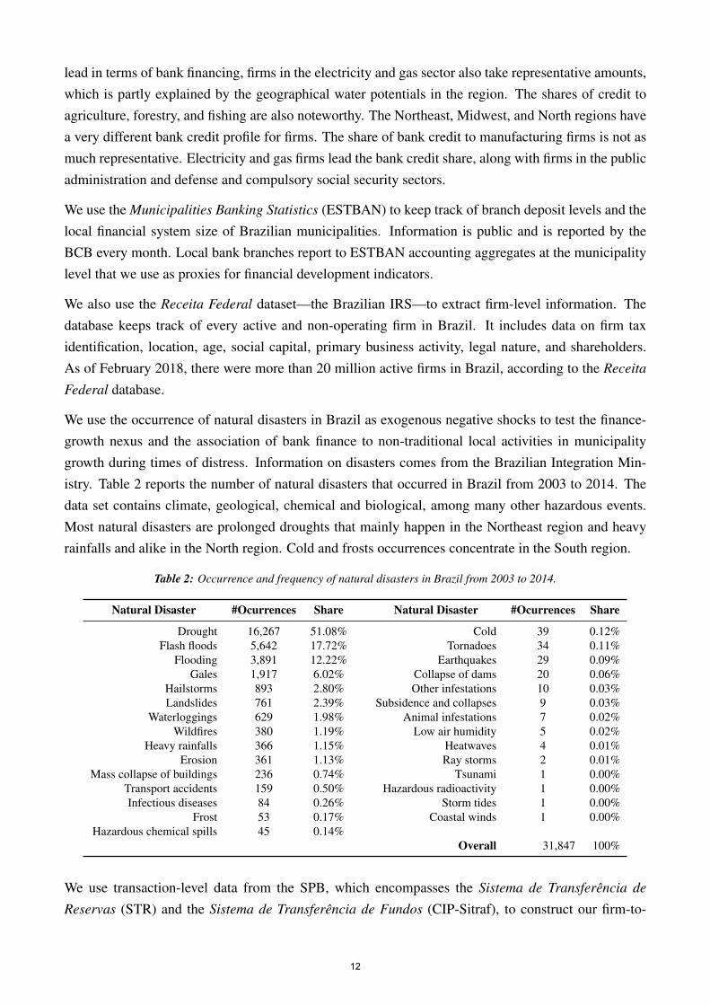
We use the occurrence of natural disasters in Brazil as exogenous negative shocks to test the finance-growth nexus and the association of bank finance to non-traditional local activities in municipalitygrowth during times of distress. Information on disasters comes from the Brazilian Integration Min-istry. Table 2 reports the number of natural disasters that occurred in Brazil from 2003 to 2014. Thedata set contains climate, geological, chemical and biological, among many other hazardous events.Most natural disasters are prolonged droughts that mainly happen in the Northeast region and heavyrainfalls and alike in the North region. Cold and frosts occurrences concentrate in the South region.
Table 2: Occurrence and frequency of natural disasters in Brazil from 2003 to 2014.
Natural Disaster #Ocurrences Share Natural Disaster #Ocurrences Share
Drought 16,267 51.08% Cold 39 0.12%Flash floods 5,642 17.72% Tornadoes 34 0.11%
Flooding 3,891 12.22% Earthquakes 29 0.09%Gales 1,917 6.02% Collapse of dams 20 0.06%
Hailstorms 893 2.80% Other infestations 10 0.03%Landslides 761 2.39% Subsidence and collapses 9 0.03%
Waterloggings 629 1.98% Animal infestations 7 0.02%Wildfires 380 1.19% Low air humidity 5 0.02%
Heavy rainfalls 366 1.15% Heatwaves 4 0.01%Erosion 361 1.13% Ray storms 2 0.01%
Mass collapse of buildings 236 0.74% Tsunami 1 0.00%Transport accidents 159 0.50% Hazardous radioactivity 1 0.00%Infectious diseases 84 0.26% Storm tides 1 0.00%
Frost 53 0.17% Coastal winds 1 0.00%Hazardous chemical spills 45 0.14%
Overall 31,847 100%
We use transaction-level data from the SPB, which encompasses the Sistema de Transferencia de
Reservas (STR) and the Sistema de Transferencia de Fundos (CIP-Sitraf), to construct our firm-to-
12
firm network.14 The BCB maintains both STR and CIP-Sitraf, which are real-time gross settlementpayment systems that record electronic interbank transactions in Brazil.15 This is a high-frequency dataset that provides information on the exact time of the transaction, the identification of the payer andreceiver of the money, the purpose of the transaction,16 and the respective branches of their accounts.
The payment transfers data has about 410 million transactions with a total commercial trading value ofR$ 48 trillion among firms between January 2003 and December 2014. To get a sense of the transactedvolume, this corresponds to more than 20 times the annual nominal GDP of Brazil in 2014. Ourpayment data contains about 9 million firm local branches that transacted at least once, which is almosthalf of the total universe of firms registered at the Receita Federal database. The difference that weobserve in the data to this firm catalog is mostly due to individual microentrepreneurs, which are firmsof a single employee, the owner, that mostly offer services to the final customer and pay their inputsand receive their revenues by cash or debit cards.
We classify firms as suppliers or customers by following the direction of money transfers. Suppliersare receivers of money and therefore reside in the creditor side of the monetary transaction. Customerfirms are the payers of the money and are on the debtor side of the transaction. This identificationpermits us to navigate through the entire supply chain in Brazil. For instance, by following the chainsof the supplier to the customer, we navigate downstream in the supply chain.
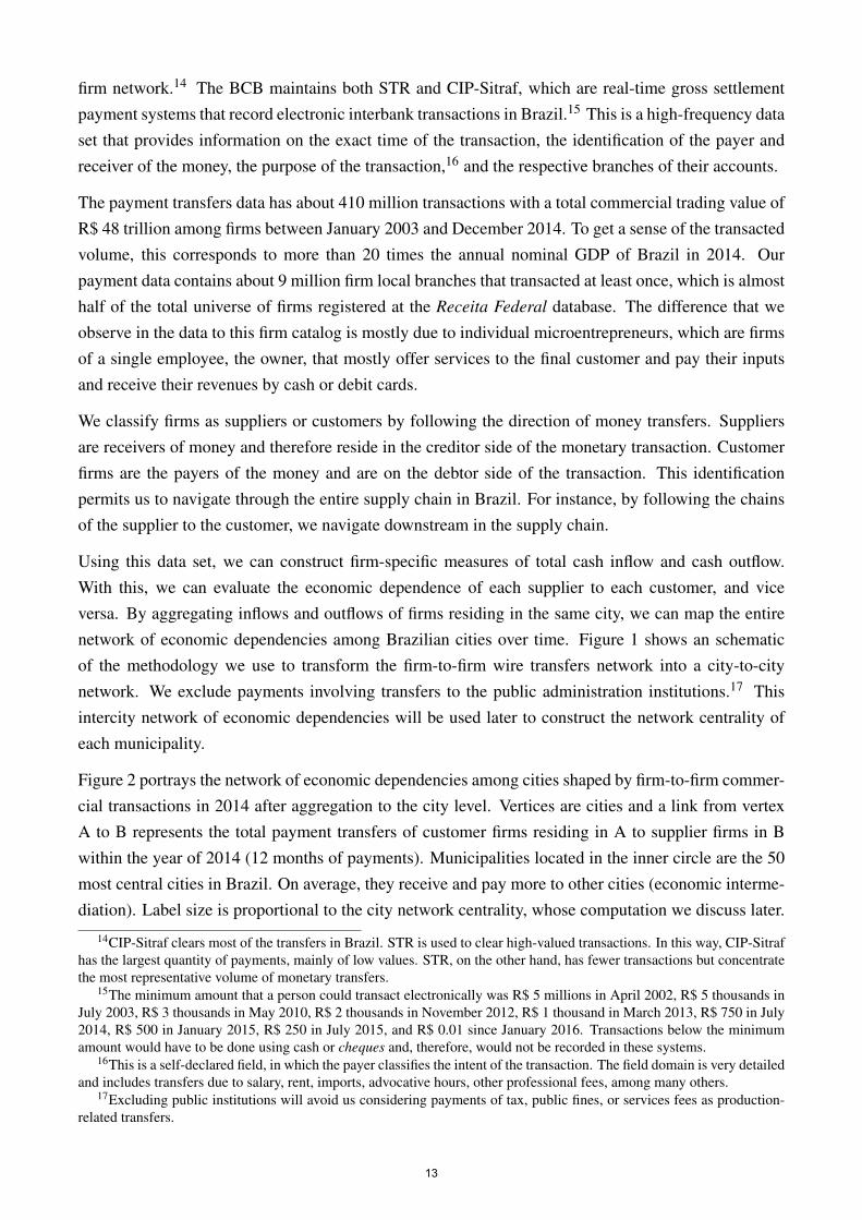
Using this data set, we can construct firm-specific measures of total cash inflow and cash outflow.With this, we can evaluate the economic dependence of each supplier to each customer, and viceversa. By aggregating inflows and outflows of firms residing in the same city, we can map the entirenetwork of economic dependencies among Brazilian cities over time. Figure 1 shows an schematicof the methodology we use to transform the firm-to-firm wire transfers network into a city-to-citynetwork. We exclude payments involving transfers to the public administration institutions.17 Thisintercity network of economic dependencies will be used later to construct the network centrality ofeach municipality.
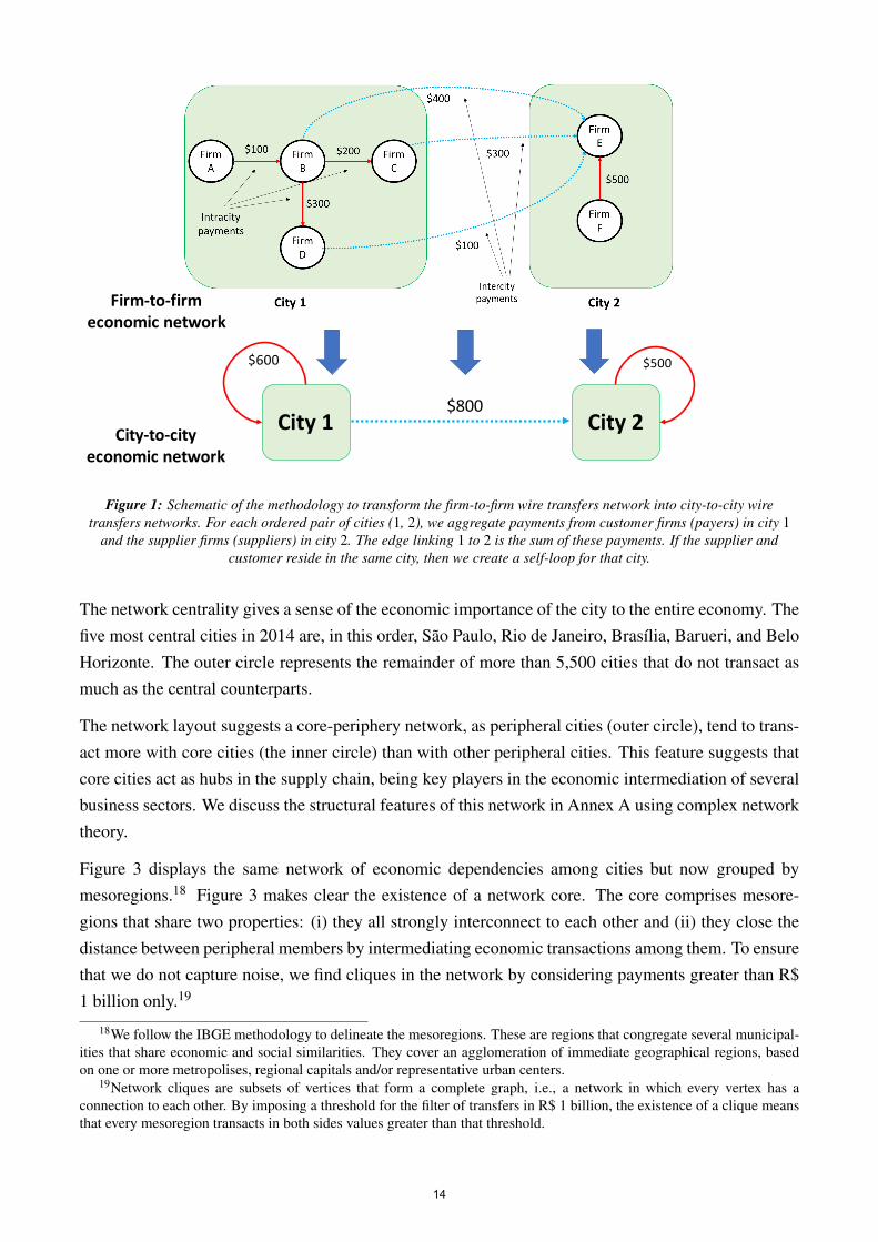
Figure 2 portrays the network of economic dependencies among cities shaped by firm-to-firm commer-cial transactions in 2014 after aggregation to the city level. Vertices are cities and a link from vertexA to B represents the total payment transfers of customer firms residing in A to supplier firms in Bwithin the year of 2014 (12 months of payments). Municipalities located in the inner circle are the 50most central cities in Brazil. On average, they receive and pay more to other cities (economic interme-diation). Label size is proportional to the city network centrality, whose computation we discuss later.
14CIP-Sitraf clears most of the transfers in Brazil. STR is used to clear high-valued transactions. In this way, CIP-Sitrafhas the largest quantity of payments, mainly of low values. STR, on the other hand, has fewer transactions but concentratethe most representative volume of monetary transfers.
15The minimum amount that a person could transact electronically was R$ 5 millions in April 2002, R$ 5 thousands inJuly 2003, R$ 3 thousands in May 2010, R$ 2 thousands in November 2012, R$ 1 thousand in March 2013, R$ 750 in July2014, R$ 500 in January 2015, R$ 250 in July 2015, and R$ 0.01 since January 2016. Transactions below the minimumamount would have to be done using cash or cheques and, therefore, would not be recorded in these systems.
16This is a self-declared field, in which the payer classifies the intent of the transaction. The field domain is very detailedand includes transfers due to salary, rent, imports, advocative hours, other professional fees, among many others.
17Excluding public institutions will avoid us considering payments of tax, public fines, or services fees as production-related transfers.
13
City 1 City 2
$600 $500
$800
Firm-to-firm economic network
City-to-city economic network
Figure 1: Schematic of the methodology to transform the firm-to-firm wire transfers network into city-to-city wiretransfers networks. For each ordered pair of cities (1, 2), we aggregate payments from customer firms (payers) in city 1
and the supplier firms (suppliers) in city 2. The edge linking 1 to 2 is the sum of these payments. If the supplier andcustomer reside in the same city, then we create a self-loop for that city.
The network centrality gives a sense of the economic importance of the city to the entire economy. Thefive most central cities in 2014 are, in this order, Sao Paulo, Rio de Janeiro, Brasılia, Barueri, and BeloHorizonte. The outer circle represents the remainder of more than 5,500 cities that do not transact asmuch as the central counterparts.
The network layout suggests a core-periphery network, as peripheral cities (outer circle), tend to trans-act more with core cities (the inner circle) than with other peripheral cities. This feature suggests thatcore cities act as hubs in the supply chain, being key players in the economic intermediation of severalbusiness sectors. We discuss the structural features of this network in Annex A using complex networktheory.
Figure 3 displays the same network of economic dependencies among cities but now grouped bymesoregions.18 Figure 3 makes clear the existence of a network core. The core comprises mesore-gions that share two properties: (i) they all strongly interconnect to each other and (ii) they close thedistance between peripheral members by intermediating economic transactions among them. To ensurethat we do not capture noise, we find cliques in the network by considering payments greater than R$1 billion only.19
18We follow the IBGE methodology to delineate the mesoregions. These are regions that congregate several municipal-ities that share economic and social similarities. They cover an agglomeration of immediate geographical regions, basedon one or more metropolises, regional capitals and/or representative urban centers.
19Network cliques are subsets of vertices that form a complete graph, i.e., a network in which every vertex has aconnection to each other. By imposing a threshold for the filter of transfers in R$ 1 billion, the existence of a clique meansthat every mesoregion transacts in both sides values greater than that threshold.
14
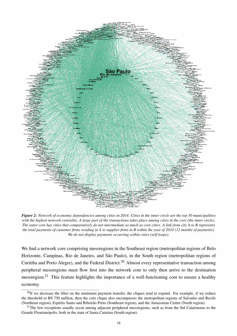
Figure 2: Network of economic dependencies among cities in 2014. Cities in the inner circle are the top 50 municipalitieswith the highest network centrality. A large part of the transactions takes place among cities in the core (the inner circle).The outer core has cities that comparatively do not intermediate as much as core cities. A link from city A to B representsthe total payments of customer firms residing in A to supplier firms in B within the year of 2014 (12 months of payments).
We do not display payments occurring within cities (self-loops).
We find a network core comprising mesoregions in the Southeast region (metropolitan regions of BeloHorizonte, Campinas, Rio de Janeiro, and Sao Paulo), in the South region (metropolitan regions ofCuritiba and Porto Alegre), and the Federal District.20 Almost every representative transaction amongperipheral mesoregions must flow first into the network core to only then arrive to the destinationmesoregion.21 This feature highlights the importance of a well-functioning core to ensure a healthyeconomy.
20If we decrease the filter on the minimum payment transfer, the cliques tend to expand. For example, if we reducethe threshold to R$ 750 million, then the core clique also encompasses the metropolitan regions of Salvador and Recife(Northeast region), Espırito Santo and Ribeirao Preto (Southeast region), and the Amazonian Centre (North region).
21The few exceptions usually occur among adjacent peripheral mesoregions, such as from the Sul Catarinense to theGrande Floarianopolis, both in the state of Santa Catarina (South region).
15
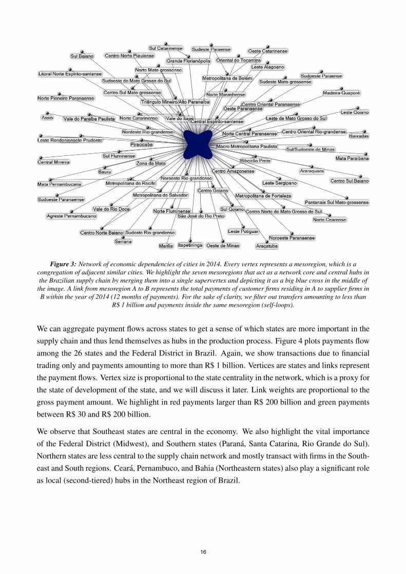
Figure 3: Network of economic dependencies of cities in 2014. Every vertex represents a mesoregion, which is acongregation of adjacent similar cities. We highlight the seven mesoregions that act as a network core and central hubs inthe Brazilian supply chain by merging them into a single supervertex and depicting it as a big blue cross in the middle of
the image. A link from mesoregion A to B represents the total payments of customer firms residing in A to supplier firms inB within the year of 2014 (12 months of payments). For the sake of clarity, we filter out transfers amounting to less than
R$ 1 billion and payments inside the same mesoregion (self-loops).
We can aggregate payment flows across states to get a sense of which states are more important in thesupply chain and thus lend themselves as hubs in the production process. Figure 4 plots payments flowamong the 26 states and the Federal District in Brazil. Again, we show transactions due to financialtrading only and payments amounting to more than R$ 1 billion. Vertices are states and links representthe payment flows. Vertex size is proportional to the state centrality in the network, which is a proxy forthe state of development of the state, and we will discuss it later. Link weights are proportional to thegross payment amount. We highlight in red payments larger than R$ 200 billion and green paymentsbetween R$ 30 and R$ 200 billion.
We observe that Southeast states are central in the economy. We also highlight the vital importanceof the Federal District (Midwest), and Southern states (Parana, Santa Catarina, Rio Grande do Sul).Northern states are less central to the supply chain network and mostly transact with firms in the South-east and South regions. Ceara, Pernambuco, and Bahia (Northeastern states) also play a significant roleas local (second-tiered) hubs in the Northeast region of Brazil.
16
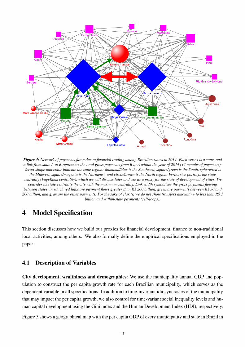
Figure 4: Network of payments flows due to financial trading among Brazilian states in 2014. Each vertex is a state, anda link from state A to B represents the total gross payments from B to A within the year of 2014 (12 months of payments).Vertex shape and color indicate the state region: diamond/blue is the Southeast, square/green is the South, sphere/red is
the Midwest, square/magenta is the Northeast, and circle/brown is the North region. Vertex size portrays the statecentrality (PageRank centrality), which we will discuss later and use as a proxy for the state of development of cities. We
consider as state centrality the city with the maximum centrality. Link width symbolizes the gross payments flowingbetween states, in which red links are payment flows greater than R$ 200 billion, green are payments between R$ 30 and
200 billion, and gray are the other payments. For the sake of clarity, we do not show transfers amounting to less than R$ 1billion and within-state payments (self-loops).
4 Model Specification
This section discusses how we build our proxies for financial development, finance to non-traditionallocal activities, among others. We also formally define the empirical specifications employed in thepaper.
4.1 Description of Variables
City development, wealthiness and demographics: We use the municipality annual GDP and pop-ulation to construct the per capita growth rate for each Brazilian municipality, which serves as thedependent variable in all specifications. In addition to time-invariant idiosyncrasies of the municipalitythat may impact the per capita growth, we also control for time-variant social inequality levels and hu-man capital development using the Gini index and the Human Development Index (HDI), respectively.
Figure 5 shows a geographical map with the per capita GDP of every municipality and state in Brazil in
17
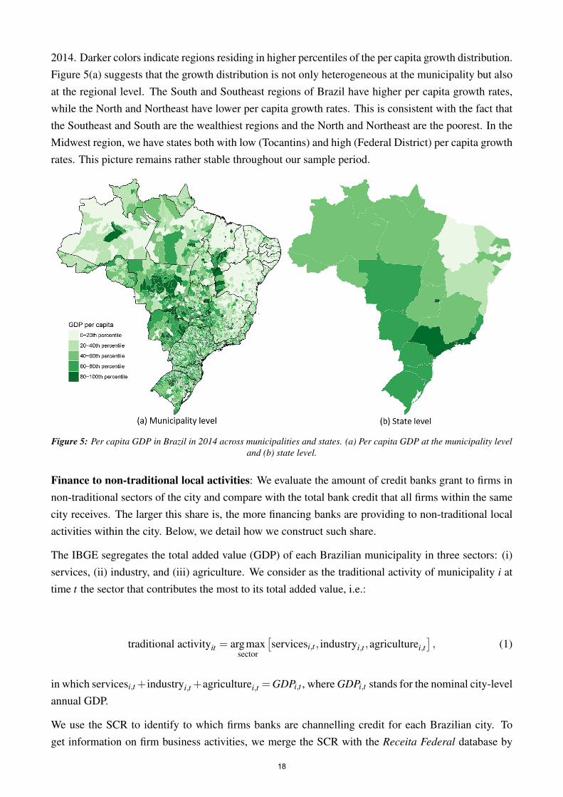
2014. Darker colors indicate regions residing in higher percentiles of the per capita growth distribution.Figure 5(a) suggests that the growth distribution is not only heterogeneous at the municipality but alsoat the regional level. The South and Southeast regions of Brazil have higher per capita growth rates,while the North and Northeast have lower per capita growth rates. This is consistent with the fact thatthe Southeast and South are the wealthiest regions and the North and Northeast are the poorest. In theMidwest region, we have states both with low (Tocantins) and high (Federal District) per capita growthrates. This picture remains rather stable throughout our sample period.
Figure 5: Per capita GDP in Brazil in 2014 across municipalities and states. (a) Per capita GDP at the municipality leveland (b) state level.
Finance to non-traditional local activities: We evaluate the amount of credit banks grant to firms innon-traditional sectors of the city and compare with the total bank credit that all firms within the samecity receives. The larger this share is, the more financing banks are providing to non-traditional localactivities within the city. Below, we detail how we construct such share.
The IBGE segregates the total added value (GDP) of each Brazilian municipality in three sectors: (i)services, (ii) industry, and (iii) agriculture. We consider as the traditional activity of municipality i attime t the sector that contributes the most to its total added value, i.e.:
traditional activityit = argmaxsector
[servicesi,t , industryi,t ,agriculturei,t
], (1)
in which servicesi,t + industryi,t +agriculturei,t =GDPi,t , where GDPi,t stands for the nominal city-levelannual GDP.
We use the SCR to identify to which firms banks are channelling credit for each Brazilian city. Toget information on firm business activities, we merge the SCR with the Receita Federal database by
18
the borrower’s tax identifier (CNPJ). We then aggregate these loan-level credit operations to city-levelcredit information over time broken down by business activities.
We then merge the city-level credit data with the IBGE by municipality code and year, so that wecan identify the traditional local activities of each city. Finally, we compute our proxy for finance tonon-traditional local activities in the municipality i at time t as:
finance to non-traditional local activitiesi,t =total crediti,t− credit to traditional activityi,t
total crediti,t,
=credit to non-traditional local activitiesi,t
total crediti,t, (2)
in which credit to traditional activityi,t is the total credit that banks grant to firms in the traditionalsector of municipality i at time t, which we identify using (1).
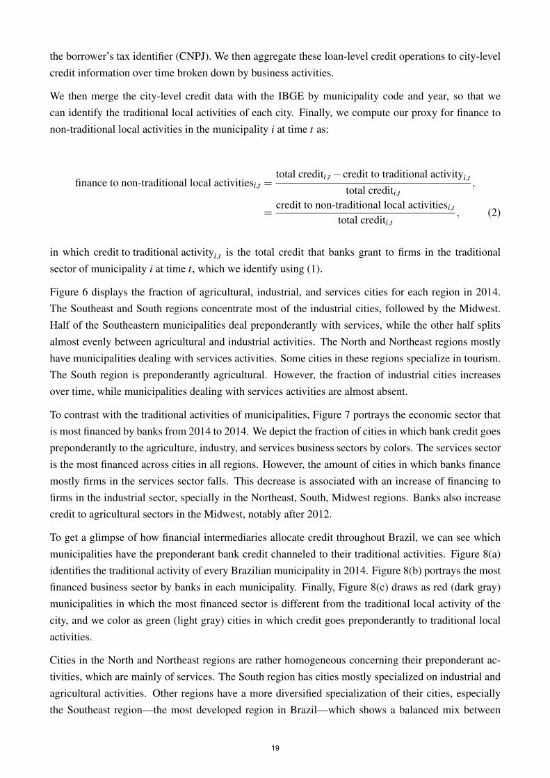
Figure 6 displays the fraction of agricultural, industrial, and services cities for each region in 2014.The Southeast and South regions concentrate most of the industrial cities, followed by the Midwest.Half of the Southeastern municipalities deal preponderantly with services, while the other half splitsalmost evenly between agricultural and industrial activities. The North and Northeast regions mostlyhave municipalities dealing with services activities. Some cities in these regions specialize in tourism.The South region is preponderantly agricultural. However, the fraction of industrial cities increasesover time, while municipalities dealing with services activities are almost absent.
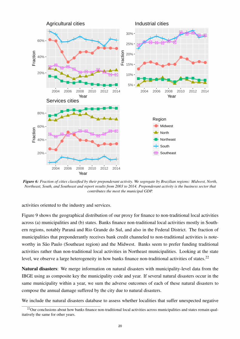
To contrast with the traditional activities of municipalities, Figure 7 portrays the economic sector thatis most financed by banks from 2014 to 2014. We depict the fraction of cities in which bank credit goespreponderantly to the agriculture, industry, and services business sectors by colors. The services sectoris the most financed across cities in all regions. However, the amount of cities in which banks financemostly firms in the services sector falls. This decrease is associated with an increase of financing tofirms in the industrial sector, specially in the Northeast, South, Midwest regions. Banks also increasecredit to agricultural sectors in the Midwest, notably after 2012.
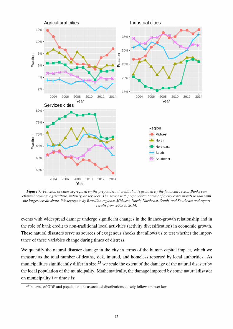
To get a glimpse of how financial intermediaries allocate credit throughout Brazil, we can see whichmunicipalities have the preponderant bank credit channeled to their traditional activities. Figure 8(a)identifies the traditional activity of every Brazilian municipality in 2014. Figure 8(b) portrays the mostfinanced business sector by banks in each municipality. Finally, Figure 8(c) draws as red (dark gray)municipalities in which the most financed sector is different from the traditional local activity of thecity, and we color as green (light gray) cities in which credit goes preponderantly to traditional localactivities.
Cities in the North and Northeast regions are rather homogeneous concerning their preponderant ac-tivities, which are mainly of services. The South region has cities mostly specialized on industrial andagricultural activities. Other regions have a more diversified specialization of their cities, especiallythe Southeast region—the most developed region in Brazil—which shows a balanced mix between
19
● ●
●
●●
● ● ●
● ● ● ●
20%
40%
60%
2004 2006 2008 2010 2012 2014
Year
Fra
ctio
n
Agricultural cities
●
● ● ●● ● ●
● ●● ● ●
5%
10%
15%
20%
25%
30%
2004 2006 2008 2010 2012 2014
Year
Fra
ctio
n
Industrial cities
● ●
●
●●
● ● ●● ● ● ●
20%
40%
60%
80%
2004 2006 2008 2010 2012 2014
Year
Fra
ctio
n
Services cities
Region
● Midwest
North
Northeast
South
Southeast
Figure 6: Fraction of cities classified by their preponderant activity. We segregate by Brazilian regions: Midwest, North,Northeast, South, and Southeast and report results from 2003 to 2014. Preponderant activity is the business sector that
contributes the most the municipal GDP.
activities oriented to the industry and services.
Figure 9 shows the geographical distribution of our proxy for finance to non-traditional local activitiesacross (a) municipalities and (b) states. Banks finance non-traditional local activities mostly in South-ern regions, notably Parana and Rio Grande do Sul, and also in the Federal District. The fraction ofmunicipalities that preponderantly receives bank credit channeled to non-traditional activities is note-worthy in Sao Paulo (Southeast region) and the Midwest. Banks seem to prefer funding traditionalactivities rather than non-traditional local activities in Northeast municipalities. Looking at the statelevel, we observe a large heterogeneity in how banks finance non-traditional activities of states.22
Natural disasters: We merge information on natural disasters with municipality-level data from theIBGE using as composite key the municipality code and year. If several natural disasters occur in thesame municipality within a year, we sum the adverse outcomes of each of these natural disasters tocompose the annual damage suffered by the city due to natural disasters.
We include the natural disasters database to assess whether localities that suffer unexpected negative
22Our conclusions about how banks finance non-traditional local activities across municipalities and states remain qual-itatively the same for other years.
20
●
●
●●
●
● ● ●●
●●
●
2%
4%
6%
8%
10%
12%
2004 2006 2008 2010 2012 2014
Year
Fra
ctio
n
Agricultural cities
● ●●
●
●
●
● ●
● ●●
●
15%
20%
25%
30%
35%
2004 2006 2008 2010 2012 2014
Year
Fra
ctio
n
Industrial cities
●● ●
● ●
●
● ●●
●●
●55%
60%
65%
70%
75%
80%
2004 2006 2008 2010 2012 2014
Year
Fra
ctio
n
Services cities
Region
● Midwest
North
Northeast
South
Southeast
Figure 7: Fraction of cities segregated by the preponderant credit that is granted by the financial sector. Banks canchannel credit to agriculture, industry, or services. The sector with preponderant credit of a city corresponds to that withthe largest credit share. We segregate by Brazilian regions: Midwest, North, Northeast, South, and Southeast and report
results from 2003 to 2014.
events with widespread damage undergo significant changes in the finance-growth relationship and inthe role of bank credit to non-traditional local activities (activity diversification) in economic growth.These natural disasters serve as sources of exogenous shocks that allows us to test whether the impor-tance of these variables change during times of distress.
We quantify the natural disaster damage in the city in terms of the human capital impact, which wemeasure as the total number of deaths, sick, injured, and homeless reported by local authorities. Asmunicipalities significantly differ in size,23 we scale the extent of the damage of the natural disaster bythe local population of the municipality. Mathematically, the damage imposed by some natural disasteron municipality i at time t is:
23In terms of GDP and population, the associated distributions closely follow a power law.
21
Figu
re8:
Pre
pond
eran
tact
iviti
esan
dcr
edit
tom
unic
ipal
ities
inB
razi
ldur
ing
2014
.(a
)Th
etr
aditi
onal
activ
ityof
ever
yB
razi
lian
mun
icip
ality
.W
eco
nsid
erth
atth
ebu
sine
ssse
ctor
that
cont
ribu
tes
the
mos
tto
GD
Pof
am
unic
ipal
ityis
itstr
aditi
onal
activ
ity.
(b)
The
mos
tfina
nced
busi
ness
sect
orby
bank
sin
each
mun
icip
ality
.(c
)M
atch
orm
ism
atch
betw
een
the
trad
ition
allo
cala
ctiv
ityan
dth
em
ostfi
nanc
edbu
sine
ssse
ctor
inea
chB
razi
lian
mun
icip
ality
.Mis
mat
ches
are
inre
d(d
ark
gray
)and
mat
ches
are
ingr
een
(lig
htgr
ay).
22
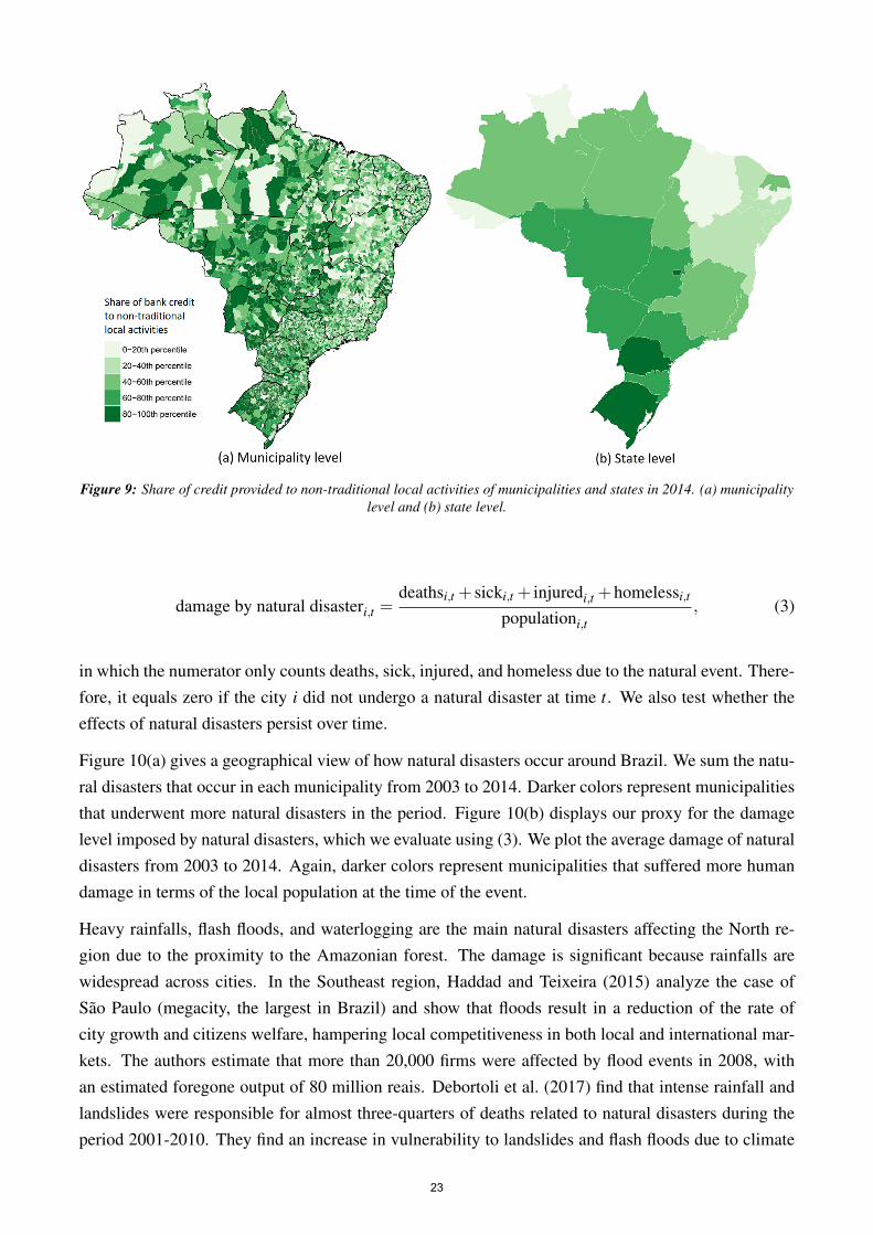
Figure 9: Share of credit provided to non-traditional local activities of municipalities and states in 2014. (a) municipalitylevel and (b) state level.
damage by natural disasteri,t =deathsi,t + sicki,t + injuredi,t +homelessi,t
populationi,t, (3)
in which the numerator only counts deaths, sick, injured, and homeless due to the natural event. There-fore, it equals zero if the city i did not undergo a natural disaster at time t. We also test whether theeffects of natural disasters persist over time.
Figure 10(a) gives a geographical view of how natural disasters occur around Brazil. We sum the natu-ral disasters that occur in each municipality from 2003 to 2014. Darker colors represent municipalitiesthat underwent more natural disasters in the period. Figure 10(b) displays our proxy for the damagelevel imposed by natural disasters, which we evaluate using (3). We plot the average damage of naturaldisasters from 2003 to 2014. Again, darker colors represent municipalities that suffered more humandamage in terms of the local population at the time of the event.
Heavy rainfalls, flash floods, and waterlogging are the main natural disasters affecting the North re-gion due to the proximity to the Amazonian forest. The damage is significant because rainfalls arewidespread across cities. In the Southeast region, Haddad and Teixeira (2015) analyze the case ofSao Paulo (megacity, the largest in Brazil) and show that floods result in a reduction of the rate ofcity growth and citizens welfare, hampering local competitiveness in both local and international mar-kets. The authors estimate that more than 20,000 firms were affected by flood events in 2008, withan estimated foregone output of 80 million reais. Debortoli et al. (2017) find that intense rainfall andlandslides were responsible for almost three-quarters of deaths related to natural disasters during theperiod 2001-2010. They find an increase in vulnerability to landslides and flash floods due to climate
23
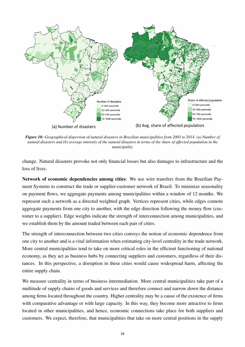
Figure 10: Geographical dispersion of natural disasters in Brazilian municipalities from 2003 to 2014. (a) Number ofnatural disasters and (b) average intensity of the natural disasters in terms of the share of affected population in the
municipality.
change. Natural disasters provoke not only financial losses but also damages to infrastructure and theloss of lives.
Network of economic dependencies among cities: We use wire transfers from the Brazilian Pay-ment Systems to construct the trade or supplier-customer network of Brazil. To minimize seasonalityon payment flows, we aggregate payments among municipalities within a window of 12 months. Werepresent such a network as a directed weighted graph. Vertices represent cities, while edges connoteaggregate payments from one city to another, with the edge direction following the money flow (cus-tomer to a supplier). Edge weights indicate the strength of interconnection among municipalities, andwe establish them by the amount traded between each pair of cities.
The strength of interconnection between two cities conveys the notion of economic dependence fromone city to another and is a vital information when estimating city-level centrality in the trade network.More central municipalities tend to take on more critical roles in the efficient functioning of nationaleconomy, as they act as business hubs by connecting suppliers and customers, regardless of their dis-tances. In this perspective, a disruption in these cities would cause widespread harm, affecting theentire supply chain.
We measure centrality in terms of business intermediation. More central municipalities take part of amultitude of supply chains of goods and services and therefore connect and narrow down the distanceamong firms located throughout the country. Higher centrality may be a cause of the existence of firmswith comparative advantage or with large capacity. In this way, they become more attractive to firmslocated in other municipalities, and hence, economic connections take place for both suppliers andcustomers. We expect, therefore, that municipalities that take on more central positions in the supply
24
chain network will be at more advanced stages of development from an economic point of view.
By using the network centrality as a proxy for the municipality state of development, we can testSchumpeter’s theory over the finance-growth nexus. In his view, banks are crucial in municipalitiesat their initial stage of economic development, for they serve as the main engines to leverage growth,mainly because of the absence of other funding sources.
In contrast, in municipalities at advanced states of economic development, the revenue accrued fromthe firm production may finance its investments and hence, growth. Besides, firms in later stages ofdevelopment have access to other funding markets, such as capital or bond markets. That is, the roleof banks in fostering economic growth becomes secondary. We also test whether the influence ofbank financing of non-traditional local activities on economic growth depends on the current stage ofdevelopment of the city.
As a robustness test, we also use the Human Development Index (HDI) as a proxy for the stage ofdevelopment of municipalities. Since HDI captures income, health, and education of the population,the rationale is that cities with HDI are likely to be in more advanced stages of development. Thisproxy is another way of looking at the stage of development from a human capital viewpoint. Ourresults remain the same.
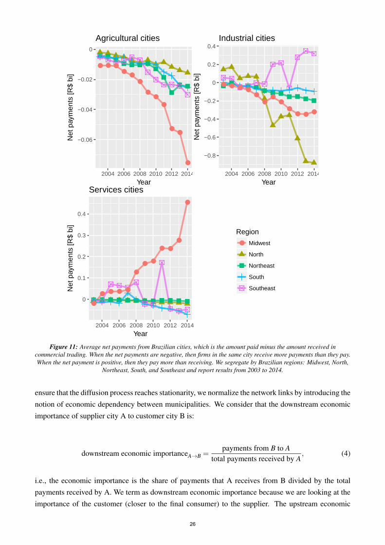
Municipalities in Brazil have very peculiar profiles in terms of their necessity of outputs and inputsfrom other cities, which depend on their traditional activities, geographical regions, the location theystand in the supply chain, their current stage of development and also their geographic and economicneighbors. Figure 11 shows the average net payments from Brazilian cities, which is the amount paidfor inputs minus the amount received for outputs in commercial trading. When the net payments arenegative, then firms in the same city receive more payments than they pay on average. Conversely,when the net payment is positive, then they pay more than receive.
Agricultural cities receive more than pay to other Brazilian cities over time, which is consistent withtheir first-stage position in the supply chain and also the increasing modernization of agricultural pro-cesses followed by gains of scale. The trend is more notable in the Midwest than in other regions.Industrial cities show high heterogeneity in their receivables and payables. On the other hand, theNorth region receives more from other municipalities than it pays over time. Such a region has theZona Franca de Manaus, which is a delimited zone that enjoys tax benefits and export facilities in anattempt to foster modernization and attract new companies in the vicinities. The Southeast region, incontrast, pays more than receives over time, partly because it contains a large number of final retailers.Cities oriented to the services sector are overall with zero net payments, except for the Midwest, whichpays a lot more than receive, especially the Federal District, which imports services from other cities.
We compute the network centrality using Google PageRank. PageRank goes beyond the local impor-tance of a city. A city will have significant PageRank only if it has many neighboring cities that havesignificant PageRank themselves. That is, it is not sufficient to establish commercial flows with manycities. It becomes imperative that these neighbors are central as well.
The recursive nature of GooglePage rank imposes some restrictions on the network topology. To
25
● ● ●●
●●
●●
●
●●
●
−0.06
−0.04
−0.02
0
2004 2006 2008 2010 2012 2014
Year
Net
pay
men
ts [R
$ bi
]
Agricultural cities
● ● ● ●●
●●
●●
● ● ●
−0.8
−0.6
−0.4
−0.2
0
0.2
0.4
2004 2006 2008 2010 2012 2014
Year
Net
pay
men
ts [R
$ bi
]
Industrial cities
●
● ● ● ●
●
● ●
● ●
●
●
0
0.1
0.2
0.3
0.4
2004 2006 2008 2010 2012 2014
Year
Net
pay
men
ts [R
$ bi
]
Services cities
Region
● Midwest
North
Northeast
South
Southeast
Figure 11: Average net payments from Brazilian cities, which is the amount paid minus the amount received incommercial trading. When the net payments are negative, then firms in the same city receive more payments than they pay.When the net payment is positive, then they pay more than receiving. We segregate by Brazilian regions: Midwest, North,
Northeast, South, and Southeast and report results from 2003 to 2014.
ensure that the diffusion process reaches stationarity, we normalize the network links by introducing thenotion of economic dependency between municipalities. We consider that the downstream economicimportance of supplier city A to customer city B is:
downstream economic importanceA→B =payments from B to A
total payments received by A, (4)
i.e., the economic importance is the share of payments that A receives from B divided by the totalpayments received by A. We term as downstream economic importance because we are looking at theimportance of the customer (closer to the final consumer) to the supplier. The upstream economic
26
importance is the reverse of this definition: it is the importance of the supplier A to cash outflows ofcustomer B. Equation (4) ensures that the weighted adjacency matrix of the graph has all entries in therange [0,1], and therefore the PageRank diffusion process is stationary (Silva and Zhao (2016)). Thisis an important transformation to assure well-defined centrality measures for every city (vertex) in thenetwork.
Figure 12 depicts the geographical dispersion of the network centrality of Brazilian cities in 2014. Aswe can see, there is significant heterogeneity in the degree of centrality of Brazilian municipalities.The Southeastern and Southern regions of Brazil are among the most central cities in Brazil. Thereare also relevant municipalities in other regions, mainly the state capitals, because they require manyinputs from others to be able to offer their goods and services. This considerable heterogeneity andspread throughout the national territory makes the Brazilian case as exciting as the object of study.
Classical financial development indicators: We expect the finance-growth nexus to hold at the mu-nicipality level: financial development helps drive economic growth. To confer robustness to ourfindings, we include in our regressions three proxies for financial development: (i) Credit/GDP, (ii)Deposits/GDP, and (iii) Financial System Size/GDP. We aggregate these ratios by city level. The creditrelates to the total outstanding credit to firms situated in the same city, deposits relate to the totalamount of private deposits both by individuals and firms in local bank branches, the financial systemsize is the sum of the total assets of every bank branch based at the city, and GDP is the nominalcity-level annual GDP.
Following recent work on the finance-growth nexus, financial development helps spur economic growthbut only up to a limit. Too much credit can lead to excessive indebtedness of both individuals and firmsand therefore may backfire to banks in the form of defaults. In an extreme credit-taking scenario,banks may relax screening procedures, increasing provisioning levels, and thus the cost of the creditoperation. In this way, following the standard in the literature, we also include the square of our proxiesfor financial development to empirically test whether there is a non-linear effect.
Table 3 compiles the variables included in the model specification and the associated source that wecollected the data. In Table 4, we present summary statistics for the variables that we use in oureconometric specification. We present the number of observations (N), mean, standard deviation (SD),5th percentile (P5), 25th percentile (P25), median, 75th percentile (P75), 95th percentile (P95), theminimum (Min) and maximum (Max) values.
4.2 Econometric Specification
We employ as dependent variable the per capita growth rate for each municipality i ∈ {1,2, . . . ,n},in which n is the number of municipalities in Brazil. The growth rate is computed as the differencein log of per capita GDP between periods t and t− 1, t ∈ {2003, . . . ,2014}. We use as independentvariables proxies for financial development, such as the outstanding credit to firms, total deposits, andfinancial system size (the sum of total assets), all as a share of the municipality’s GDP. We also includethe finance to non-traditional local activities indicator—our variable of interest—in the econometric
27

Tabl
e3:
Des
crip
tion
ofva
riab
les.
All
vari
able
sar
ere
late
dto
city
-lev
elm
easu
res.
Vari
able
Des
crip
tion
Sour
ce
Per
capi
tagr
owth
ln( 1
+Pe
rcap
itaG
DP t
Perc
apita
GD
P t−
1
)IB
GE
Fina
nce
tono
n-tr
aditi
onal
ln(1
+sh
are
ofcr
edit
tono
n-tr
aditi
onal
activ
ities)
Bra
zilia
nC
redi
tReg
istr
ylo
cala
ctiv
ities
(BC
B)
Cre
dit/
GD
Pln(1
+ou
tsta
ndin
gpr
ivat
ecr
edit
GD
P)
Bra
zilia
nC
redi
tReg
istr
y(B
CB
)
Dep
osits
/GD
Pln( 1
+to
talp
rivat
ede
posi
tsin
the
bank
ing
syst
emG
DP
)B
anki
ngSt
atis
tics
(BC
B)
Fina
ncia
lSys
tem
Size
/GD
Pln( 1
+to
tala
sset
sof
city
bank
bran
ches
GD
P
)B
anki
ngSt
atis
tics
(BC
B)
Shar
eof
affe
cted
pop
bydi
sast
erln( 1
+#d
eath
s+#s
ick+
#inj
ured+
#hom
eles
sPo
pula
tion
)B
razi
lian
Inte
grat
ion
Min
istr
y
Net
wor
kce
ntra
lity
ln(1
+C
ity’s
Page
Ran
k)B
razi
lian
Paym
ents
Syst
em(B
CB
)
Eco
nom
icsp
illov
erln( 1
+∑
j∈ne
ighb
orim
port
ance
jnet
wor
kce
ntra
lity
j)B
razi
lian
Paym
ents
Syst
em(B
CB
)
Geo
grap
hic
spill
over
max
j∈m
esor
egio
nln( 1
+ne
twor
kce
ntra
lity
j)B
razi
lian
Paym
ents
Syst
em(B
CB
)
Gin
iIn
equa
lity
inde
xIB
GE
HD
IH
uman
Dev
elop
men
tInd
exIB
GE
Incl
udes
inco
me,
educ
atio
nan
dhe
alth
28
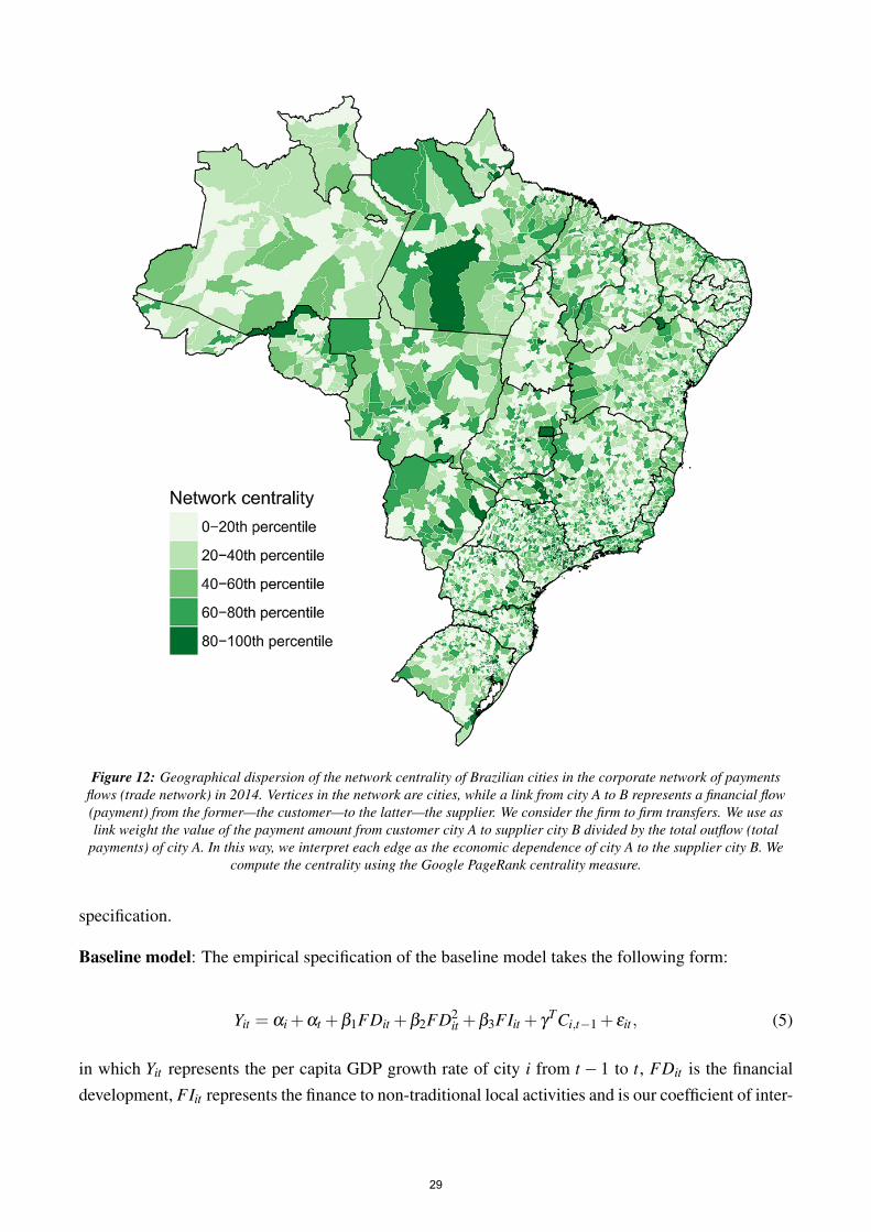
Figure 12: Geographical dispersion of the network centrality of Brazilian cities in the corporate network of paymentsflows (trade network) in 2014. Vertices in the network are cities, while a link from city A to B represents a financial flow(payment) from the former—the customer—to the latter—the supplier. We consider the firm to firm transfers. We use aslink weight the value of the payment amount from customer city A to supplier city B divided by the total outflow (total
payments) of city A. In this way, we interpret each edge as the economic dependence of city A to the supplier city B. Wecompute the centrality using the Google PageRank centrality measure.
specification.
Baseline model: The empirical specification of the baseline model takes the following form:
Yit = αi +αt +β1FDit +β2FD2it +β3FIit + γ
TCi,t−1 + εit , (5)
in which Yit represents the per capita GDP growth rate of city i from t− 1 to t, FDit is the financialdevelopment, FIit represents the finance to non-traditional local activities and is our coefficient of inter-
29
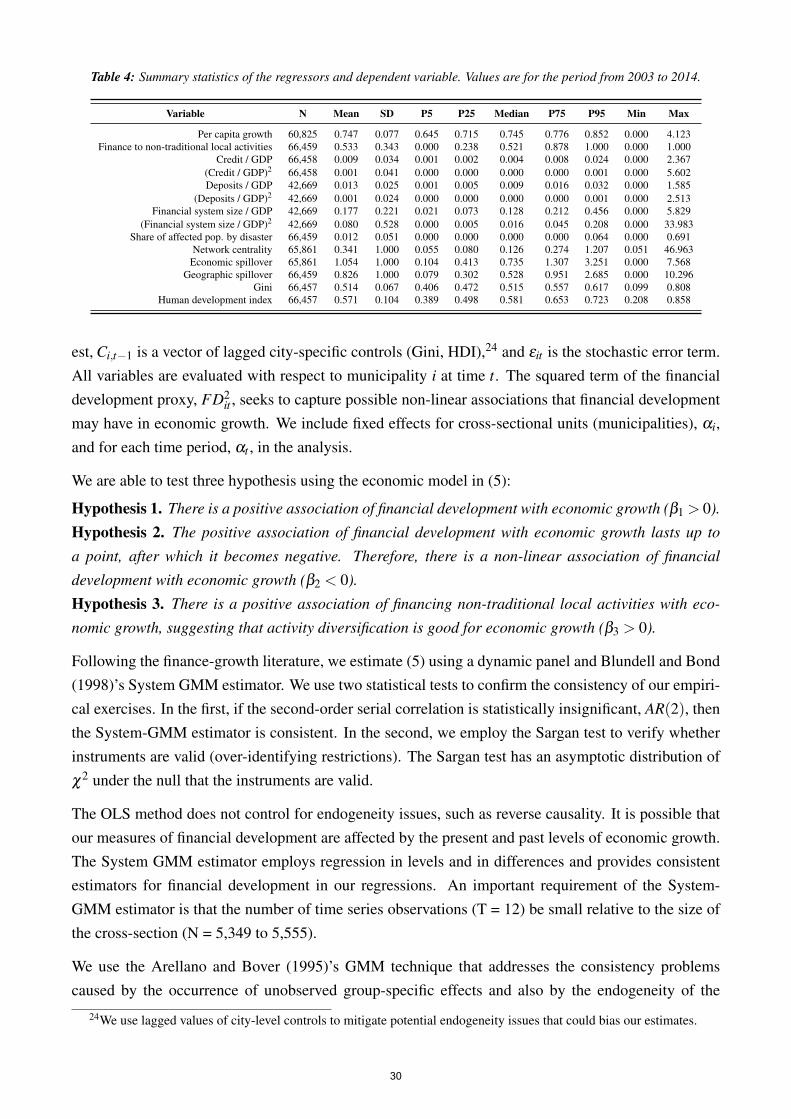
Table 4: Summary statistics of the regressors and dependent variable. Values are for the period from 2003 to 2014.
Variable N Mean SD P5 P25 Median P75 P95 Min Max
Per capita growth 60,825 0.747 0.077 0.645 0.715 0.745 0.776 0.852 0.000 4.123Finance to non-traditional local activities 66,459 0.533 0.343 0.000 0.238 0.521 0.878 1.000 0.000 1.000
Credit / GDP 66,458 0.009 0.034 0.001 0.002 0.004 0.008 0.024 0.000 2.367(Credit / GDP)2 66,458 0.001 0.041 0.000 0.000 0.000 0.000 0.001 0.000 5.602Deposits / GDP 42,669 0.013 0.025 0.001 0.005 0.009 0.016 0.032 0.000 1.585
(Deposits / GDP)2 42,669 0.001 0.024 0.000 0.000 0.000 0.000 0.001 0.000 2.513Financial system size / GDP 42,669 0.177 0.221 0.021 0.073 0.128 0.212 0.456 0.000 5.829
(Financial system size / GDP)2 42,669 0.080 0.528 0.000 0.005 0.016 0.045 0.208 0.000 33.983Share of affected pop. by disaster 66,459 0.012 0.051 0.000 0.000 0.000 0.000 0.064 0.000 0.691
Network centrality 65,861 0.341 1.000 0.055 0.080 0.126 0.274 1.207 0.051 46.963Economic spillover 65,861 1.054 1.000 0.104 0.413 0.735 1.307 3.251 0.000 7.568
Geographic spillover 66,459 0.826 1.000 0.079 0.302 0.528 0.951 2.685 0.000 10.296Gini 66,457 0.514 0.067 0.406 0.472 0.515 0.557 0.617 0.099 0.808
Human development index 66,457 0.571 0.104 0.389 0.498 0.581 0.653 0.723 0.208 0.858
est, Ci,t−1 is a vector of lagged city-specific controls (Gini, HDI),24 and εit is the stochastic error term.All variables are evaluated with respect to municipality i at time t. The squared term of the financialdevelopment proxy, FD2
it , seeks to capture possible non-linear associations that financial developmentmay have in economic growth. We include fixed effects for cross-sectional units (municipalities), αi,and for each time period, αt , in the analysis.
We are able to test three hypothesis using the economic model in (5):
Hypothesis 1. There is a positive association of financial development with economic growth (β1 > 0).
Hypothesis 2. The positive association of financial development with economic growth lasts up to
a point, after which it becomes negative. Therefore, there is a non-linear association of financial
development with economic growth (β2 < 0).
Hypothesis 3. There is a positive association of financing non-traditional local activities with eco-
nomic growth, suggesting that activity diversification is good for economic growth (β3 > 0).
Following the finance-growth literature, we estimate (5) using a dynamic panel and Blundell and Bond(1998)’s System GMM estimator. We use two statistical tests to confirm the consistency of our empiri-cal exercises. In the first, if the second-order serial correlation is statistically insignificant, AR(2), thenthe System-GMM estimator is consistent. In the second, we employ the Sargan test to verify whetherinstruments are valid (over-identifying restrictions). The Sargan test has an asymptotic distribution ofχ2 under the null that the instruments are valid.
The OLS method does not control for endogeneity issues, such as reverse causality. It is possible thatour measures of financial development are affected by the present and past levels of economic growth.The System GMM estimator employs regression in levels and in differences and provides consistentestimators for financial development in our regressions. An important requirement of the System-GMM estimator is that the number of time series observations (T = 12) be small relative to the size ofthe cross-section (N = 5,349 to 5,555).
We use the Arellano and Bover (1995)’s GMM technique that addresses the consistency problemscaused by the occurrence of unobserved group-specific effects and also by the endogeneity of the
24We use lagged values of city-level controls to mitigate potential endogeneity issues that could bias our estimates.
30
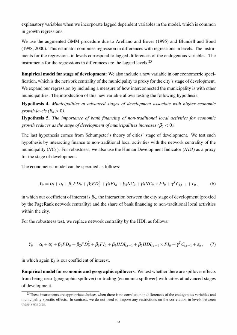
explanatory variables when we incorporate lagged dependent variables in the model, which is commonin growth regressions.
We use the augmented GMM procedure due to Arellano and Bover (1995) and Blundell and Bond(1998, 2000). This estimator combines regression in differences with regressions in levels. The instru-ments for the regressions in levels correspond to lagged differences of the endogenous variables. Theinstruments for the regressions in differences are the lagged levels.25
Empirical model for stage of development: We also include a new variable in our econometric speci-fication, which is the network centrality of the municipality to proxy for the city’s stage of development.We expand our regression by including a measure of how interconnected the municipality is with othermunicipalities. The introduction of this new variable allows testing the following hypothesis:
Hypothesis 4. Municipalities at advanced stages of development associate with higher economic
growth levels (β4 > 0).
Hypothesis 5. The importance of bank financing of non-traditional local activities for economic
growth reduces as the stage of development of municipalities increases (β5 < 0).
The last hypothesis comes from Schumpeter’s theory of cities’ stage of development. We test suchhypothesis by interacting finance to non-traditional local activities with the network centrality of themunicipality (NCit). For robustness, we also use the Human Development Indicator (HDI) as a proxyfor the stage of development.
The econometric model can be specified as follows:
Yit = αi +αt +β1FDit +β2FD2it +β3FIit +β4NCit +β5NCit×FIit + γ
TCi,t−1 + εit , (6)
in which our coefficient of interest is β5, the interaction between the city stage of development (proxiedby the PageRank network centrality) and the share of bank financing to non-traditional local activitieswithin the city.
For the robustness test, we replace network centrality by the HDI, as follows:
Yit = αi +αt +β1FDit +β2FD2it +β3FIit +β4HDIi,t−1 +β5HDIi,t−1×FIit + γ
TCi,t−1 + εit , (7)
in which again β5 is our coefficient of interest.
Empirical model for economic and geographic spillovers: We test whether there are spillover effectsfrom being near (geographic spillover) or trading (economic spillover) with cities at advanced stagesof development.
25These instruments are appropriate choices when there is no correlation in differences of the endogenous variables andmunicipality-specific effects. In contrast, we do not need to impose any restrictions on the correlation in levels betweenthese variables.
31
To test for geographic spillover effects, we check whether cities in mesoregions containing cities atadvanced stages of development associate with higher economic growth rates. For all cities withina mesoregion, the potential geographic spillover effect is given by the city with maximum stage ofdevelopment, i.e., network centrality, in that same mesoregion. For this reference city with maximumnetwork centrality, we set the geographic spillover as zero.
To test for economic spillover effects, we verify how cities transact with each other. We term as theeconomic spillover that municipality i receives the average of network centralities of all cities j withwhich city i transacts weighted by the amount of payments i pays to each j.
The resulting econometric model is:
Yit = αi +αt +β1FDit +β2FD2it +β3FIit +β4NCit +β5NCit×FIit +δ1ESit +δ2GSit + γ
TCi,t−1 + εit ,
(8)
in which ESit is the weighted average of network centrality of all municipalities that trade with mu-nicipality i (Economic Spillover), and GSit is the mesoregion’s maximum network centrality at whichmunicipality i is located (Geographic Spillover). In case city i has the maximum network centrality inthe mesoregion, we set this term to 0. Our coefficients of interest are δ1 and δ2, which measure theassociation of economic growth and economic and geographical spillovers, respectively. With the helpof this new specification we can test the following hypotheses:
Hypothesis 6. Economic spillover: Trading with cities at advanced stages of development is associated
with higher economic growth rates (δ1 > 0).
Hypothesis 7. Geographic spillover: Residing near cities at advanced stages of development is asso-
ciated with higher economic growth rates (δ2 > 0).
4.3 Differences-in-Differences (DID) Approach
We consider natural disasters as sources of unexpected negative events to investigate whether the as-sociation between financing activity diversification and economic growth changes during times of dis-tress. We also test how the finance-growth nexus stands in this stressed situation. We should notethat the way banks finance local activity diversification and how the financial system is developedlocally are endogenous to the city economic growth. In this way, even though we use a differences-in-differences approach, we still cannot impute causal meaning to our estimates.
Natural disasters can impair business activities. In the supply side, they can affect firm productionin the form of smaller quantities of available goods and higher prices (negative production shock).In the demand side, customers of these affected firms can replace their suppliers by unaffected ones,potentially outside the disaster area. If this switching ability is perfect, the consequences of the naturaldisasters would dissipate right at suppliers and the overall economic growth of the municipality wouldnot be impaired. Natural disasters also influence the welfare of citizens and the municipality fiscal
32
conditions. Labor force can reduce and public expending can increase. If the municipal capacity ofpublic services is large enough, then these shocks would not affect economic growth. Therefore, it isan empirical question to test for the consequences for economic growth in view of natural disasters.
We consider the largest natural disasters that occurred in Brazil from 2004 to 2014.26 We filter outseasonal natural disasters, such as droughts in the Northeast region and rainfalls in the North regionwith losses roughly similar to the expected losses (historical mean). Our unit of analysis in the DIDapproach is shock-city-time. As there are multiple cities suffering natural disasters at different years,we use a pooled panel-data DID analysis, in which we center the time index at zero for each city-timethat suffered a natural disaster. Mathematically, t = 0 represents the year of occurrence of the naturaldisaster at a specific city, t = n represents n > 0 years after the shock and −n indicates n years beforethe shock. In our analysis, we use the time frame t ∈ {−4,−3, . . . ,0,1, . . . ,3}, i.e. four points before(pre-treatment) and after (post-treatment) the shock. The panel can be unbalanced, so that some shocksneed not have all time points.
We first test the implications of natural disasters on economic growth using two treatment variables: (i)a binary treatment variable BTi ∈ {0,1}, which equals one if city i has suffered a shock within the timeframe we are analyzing and zero, otherwise; and (ii) a continuous treatment variable CTi ∈ [0,1], whichtakes values equivalently to the intensity of the natural disaster within the time frame. We estimate suchintensity by evaluating the number of deaths, sick persons, injured and homeless as a ratio of the localpopulation. We formulate the following hypothesis:
Hypothesis 8. Natural disasters reduce economic growth in affected municipalities (φ0 < 0).
To mitigate potential omitted variables, we compare cities that have suffered natural disasters (treat-ment group) with clusters of similar municipalities that did not experience natural disasters (controlgroup). We use two matching strategies to identify clusters/groups of similar cities. In the first, weconsider only nearby cities, i.e., those belonging to the same mesoregion of the affected city.27 In thesecond, we not only look at the geographical neighborhood but also consider demography, economicand financial conditions to pair affected and control (similar) cities. During our matching procedure,we pair treatment and control cities using only (ex-ante) city-level characteristics immediately beforethe occurrence of the natural disaster.
For the second matching strategy, we select the Gini index and population size to pair cities with similardemography conditions. We use several indicators to cluster cities with respect to their economic andfinancial conditions. First, we capture the commercial characteristics of cities to the rest of country. Weuse the municipality dependency on external suppliers—i.e. suppliers that are not based in the samecity—and equivalently the municipality dependency on external customers. We extract this informationfrom wire payments between firms. They are given by:
26Even though we have data from 2003 to 2014, we remove shocks that took place in 2003 so that we can have at leastone point in the pre- and post-treatment periods for the diff-in-diff analysis.
27This matching strategy removes widespread natural disasters that enclose entire mesoregions. For instance, most ofthe heavy rainfalls nearby Amazonian cities are extensive, such that there are no candidate cities for the control group.These shocks, therefore, are not studied in this paper.
33
external supplier dependencyi =∑ j∈Fi ∑k∈Fi
p jk
∑ j∈Fi ∑k∈F p jk, (9)
external customer dependencyi =∑ j∈Fi ∑k∈Fi
pk j
∑ j∈Fi ∑k∈F pk j, (10)
in which p jk is the transfer amount of customer firm j to supplier firm k. The sets Fi, Fi, andF =Fi∪Fi represent all active firms inside municipality i, firms outside municipality i, and all firmsin the economy, respectively. For example, in (9), the numerator sums over payments from firms j
inside city i to firms k outside municipality i. In contrast, the denominator sums over payments from j
to every firm k in the economy, be they in city i or not. Note that firms j and k play the role of customerand supplier firms, respectively, in (9), while they assume the opposite role in (10).
We also capture the amount of economic activity of business firms with respect to the municipalityGDP. This is an important aspect in Brazil because cities receive transfers from the federal governmenteither compulsory or voluntary. Therefore, their level of economic activity relatively to its GDP cansignificant differ. For that, we compute the total transfers paid and received by firms in municipality i
in relation to the local GDP, as follows:
total paidi =∑ j∈Fi ∑k∈F p jk
GDPi, (11)
total receivedi =∑ j∈Fi ∑k∈F pk j
GDPi. (12)
We also group municipalities that share similar stages of development. We use as proxy the networkcentrality in the commercial trading network.
During the matching procedure, we discretize the continuous variables in quintiles and construct clus-ters of cities that match in every geographic, demographic, economic, and financial conditions dis-played above. We then compare within these groups how economic growth associates with activitydiversification and financial development in affected and unaffected cities.
We hypothesize that the finance-growth statistical relationship becomes stronger in municipalities thatare under distress due to natural disasters. In affected areas, firms’ creditworthiness declines, narrowingdown their funding options. In this way, firms may have to resort to bank credit, which is their availablechoice at disposal in times of distress. Despite being a more expensive funding source, bank credithelps to sustain firm’s business operations and therefore contributes to economic growth. In Brazil,this effect tends to be stronger since capital markets are underdeveloped. We formulate the followinghypothesis:
34
Hypothesis 9. The association of financial development and economic growth becomes stronger in
municipalities that are under distress (φ1 +2φ2 > 0).
Financing non-traditional local activities in times of distress does not take the same positive role asfinancial development. Cities have traditional business activities that may become impaired becauseof natural disasters. In contrast to normal times, in which traditional activities are running smoothlyand there is room for developing unexplored business within municipalities, in distressed times mu-nicipalities must recover and put together the “shattered pieces” of their traditional activities. Froman economic perspective, it is more efficient to restore their traditional activities with comparative ad-vantage. In addition, these sectors have lower information information asymmetry and then financingcosts are relatively cheaper. We test the following hypothesis:
Hypothesis 10. The association of financing non-traditional local activities and economic growth
becomes weaker in municipalities under distress (φ3 < 0).
To test for Hypotheses 8 to 10, we center the occurrence of each shock at t = 0 and use a pooledpanel-data DID analysis as follows:
Yitcs = αis +αtcs +φ0TisPts +φ1TisPtsFDis +φ2TisPtsFD2is +φ3TisPtsFIis + εitcs, (13)
in which i, t, c, s index city, time, cluster, and shock, respectively. Tis is the treatment variable that cantake the binary or continuous versions, as discussed before. This variable not only depends on the cityi but also on the shock s. In this way, the same city can be considered as treatment in one shock but ascontrol in other shocks that happen across different years. Pts is the post shock-dependent variable andequals 1 if t ≥ 0 and 0, otherwise. We do not need to add Tis and Pts individually—like in a traditionaldiff-in-diff analysis—because they would be absorbed by the fixed effects αis and αtcs, respectively.The coefficient φ0 is the treatment-post variable and hence captures the effect of natural disasters oncities economic growth (Hypothesis 8).
We also interact the treatment-post variable with the municipality ex-ante and fixed financial develop-ment and finance to non-traditional local activities values. Coefficients φ1 and φ2 capture the linearco-variation (FDis) and quadratic co-variation (FD2
is) of financial development on economic growth,respectively, in affected cities. Likewise, φ3 captures the linear association of finance to non-traditionallocal activities (FIis) and economic growth in affected cities. We denote the ex-ante and fixed financialdevelopment and finance to non-traditional local activities as FDis,t=−1 and FIis,t=−1, respectively.
The term αis represents city-shock fixed effects. Again, the interaction with the shock identifier givesmore flexibility to the model, in the sense that the idiosyncrasies of the same city are time-invariantalong the same shock but are otherwise allowed to differ across different shocks.
The term αtcs indicates fixed effects that implement our city matching strategy. These fixed effects aretime-varying and ensure that we are comparing the effects of natural disasters only within clusters ofsimilar cities. They absorb the average per capita growth rates within each cluster at each point in time.
35
Again, we interact with the shock to isolate the effects of each shock in the estimation.
5 Empirical Results
In this section, we present the main empirical findings of the paper.
5.1 Correlates of growth: financial development and activity diversification(Hypotheses 1–3)
Table 5 reports our baseline dynamic panel-data specification. We estimate Eq. (1) using per capitaGDP growth as dependent variable. In columns (1-2), we use the variable Deposits/GDP as a proxyfor financial development, whereas we use Financial System Size/GDP and Credit/GDP in columns(3–4) and (5–6) as proxies for financial development, respectively. We also run a regression with allthese financial development proxies together in columns (7–8).
The proxies for financial development—i.e., deposits in columns (1–2), financial system size in columns(3–4), and credit in columns (3–4)—are statistically significant. These results confirm our Hypothe-sis 1. In addition, by including all proxies for financial development, only the deposit variable andits squared term lose statistical significance (columns 7–8), which may reflect the pairwise positivecorrelation of deposits and credit. The positive sign of the linear financial development coefficientsindicates that financial development has a positive association with economic growth. However, suchmutualistic link between financial development and economic growth correlates positively only up toa limit. Following the literature, we capture this non-linear behavior by using squared financial de-velopment variables in the specifications. We find that the signs of the squared terms are all negative,suggesting the existence of a saturation point above which the partial correlation of financial develop-ment with economic growth becomes negative. This finding confirms our Hypothesis 2. Our findingsare in line with many cross-country studies that also report a non-linear relationship between financialdevelopment and economic growth.
The non-linearity we are able to capture regardless of the model specification may be due to a variety ofreasons. Municipalities with large, well-developed and complex financial systems may have financialintermediaries that increase their risk-taking behavior, in a more aggressive competition environment,which may have adverse effects on growth. In this case, the economy would be more prone to suf-fering from adverse fluctuations provoked by the financial sector (Rajan (2006)). There may also be asubstitution effect as the financial sector grows larger. High-skilled workers may migrate from the realsector to the financial sector, which may induce a reduction in the productivity in the real sector (Tobin(1984)).
We include our proxy for finance to non-traditional local activities in columns (2), (4), (6) and (8).Finance to non-traditional local activities remains statistically significant in all specifications with a
36
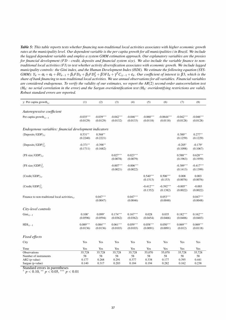
Table 5: This table reports tests whether financing non-traditional local activities associates with higher economic growthrates at the municipality level. Our dependent variable is the per capita growth for all municipalities i in Brazil. We includethe lagged dependent variable and employ a system GMM estimation approach. Our explanatory variables are the proxiesfor financial development (FD - credit, deposits and financial system size). We also include the variable finance to non-traditional local activities (FI) to test whether activity diversification associates with economic growth. We include laggedmunicipality controls: the Gini index, and the Human Development Index (HDI). We estimate the following equation (SYS-GMM): Yit = αi +αt + δYit−1 +β1FDit +β2FD2
it +β3FIit + γTCi,t−1 + εit . Our coefficient of interest is β3, which is theshare of bank financing to non-traditional local activities. We use annual observations for all variables. Financial variablesare considered endogenous. To verify the validity of our estimates, we report the AR(2) second-order autocorrelation test(H0: no serial correlation in the error) and the Sargan overidentification test (H0: overidentifying restrictions are valid).Robust standard errors are reported.
y: Per capita growthi,t (1) (2) (3) (4) (5) (6) (7) (8)
Autoregressive coefficientPer capita growthi,t−1 -0.035∗∗∗ -0.039∗∗∗ -0.042∗∗∗ -0.046∗∗∗ -0.060∗∗∗ -0.0644∗∗∗ -0.042∗∗∗ -0.046∗∗∗
(0.0129) (0.0129) (0.0132) (0.0133) (0.0118) (0.0118) (0.0128) (0.0128)
Endogenous variables: financial development indicators(Deposits/GDP)i,t 0.531∗∗ 0.568∗∗ 0.300∗∗ 0.277∗∗
(0.2240) (0.2221) (0.1259) (0.1229)
(Deposits/GDP)2i,t -0.371∗∗ -0.398∗∗ -0.205∗ -0.179∗
(0.1711) (0.1682) (0.1098) (0.1067)
(FS size/GDP)i,t 0.027∗∗∗ 0.023∗∗∗ 0.588∗∗∗ 0.628∗∗∗
(0.0078) (0.0079) (0.1963) (0.1959)
(FS size/GDP)2i,t -0.007∗∗∗ -0.006∗∗∗ -0.389∗∗∗ -0.417∗∗∗
(0.0021) (0.0022) (0.1413) (0.1399)
(Credit/GDP)i,t 0.540∗∗∗ 0.506∗∗∗ 0.008 0.003(0.1513) (0.153) (0.0076) (0.0076)
(Credit/GDP)2i,t -0.412∗∗∗ -0.392∗∗∗ -0.005∗∗ -0.003
(0.1352) (0.1382) (0.0022) (0.0022)
Finance to non-traditional local activitiesi,t 0.047∗∗∗ 0.047∗∗∗ 0.053∗∗∗ 0.047∗∗∗
(0.0047) (0.0046) (0.0048) (0.0048)
City-level controlsGinii,t−1 0.108∗ 0.099∗ 0.174∗∗∗ 0.167∗∗∗ 0.028 0.035 0.182∗∗∗ 0.162∗∗∗
(0.0596) (0.0594) (0.0362) (0.0362) (0.0454) (0.0466) (0.0406) (0.0403)
HDIi,t−1 0.089∗∗∗ 0.084∗∗∗ 0.061∗∗∗ 0.059∗∗∗ 0.058∗∗∗ 0.050∗∗∗ 0.069∗∗∗ 0.069∗∗∗
(0.0136) (0.0136) (0.0103) (0.0103) (0.0091) (0.0091) (0.012) (0.0118)
Fixed effectsCity Yes Yes Yes Yes Yes Yes Yes Yes
Time Yes Yes Yes Yes Yes Yes Yes YesObservations 35,728 35,728 35,728 35,728 55,070 55,070 35,728 35,728Number of instruments 58 58 58 58 58 58 58 58AR2 (p-value) 0.177 0.268 0.291 0.377 0.338 0.177 0.395 0.441Sargan (p-value) 0.140 0.317 0.203 0.184 0.194 0.282 0.162 0.238
Standard errors in parentheses∗ p < 0.10, ∗∗ p < 0.05, ∗∗∗ p < 0.01
37

positive sign. Thus, a one-percentage increase in the funding to non-traditional local activities (non-traditional activities) correlates to increases of the per capita growth rate by 4.7% or 5.3% withinmunicipalities. This finding confirms our Hypothesis 3.
Our results suggest that finance to non-traditional local activities strongly correlates with economicgrowth. There seems to be a complementary effect between financial development and the share offunds allocated to non-traditional activities at the municipality level.
5.2 Connection between financing non-traditional local activities and city stageof development (Hypotheses 4–5)
Cities at earlier stages of development tend to have smaller and not yet consolidated firms. Whileexternal lending for small firms is hard because financial intermediation suffers from financial frictionsdue to high information asymmetries, the average small firm may not have means of external fundingother than bank funding. In this way, the presence of banks will largely impact the business activities oflocal firms for those that need external funding and actually obtain it. This is even more pronounced forfirms exerting the non-traditional local activities of the city, in which external funding is even harderto obtain. In this scenario, we expect that any credit channeled to non-traditional local activities bestrongly associated with economic growth.
In contrast, in cities at advanced stages of development, firms tend to be larger and with consolidatedand known business portfolios. Hence, information asymmetry is lower and external funding is easier.In addition, because of their sizes, firms have more disposable capital for investments, such as accruedprofits, and therefore should rely less on bank lending. In this case we would expect that bank creditto non-preponderant activities will play a minor role in promoting further growth (auxiliary role),precisely because firms have other cheaper means of obtaining funds.
Unconditionally, cities at more advanced stages of development have more potential to prosper andtherefore tend to have higher growth rates, precisely because they have more funding options, largerfirms, better labor force, among others.
Table 6 reports our dynamic panel-data regressions using the network centrality as a proxy for the stageof development. Like the previous exercise, we document results for different proxies for financialdevelopment in each column (column 1 - deposits; column 2 - financial system size; column 3 - credit;column 4 - all financial development variables).
We see that the unconditional network centrality measure is positive and statistically significant in allspecification, suggesting cities at more advanced stages of development correlate with higher economicgrowth rates. This confirms our Hypothesis 4.
We interact the stage of development (network centrality) with the share of bank funding to non-traditional local activities to test whether banks take on an ancillary role as cities become more devel-oped. The interaction is statistically significant and negative across all specifications, suggesting thatthe association between finance to non-traditional activities and economic growth is more pronounced
38
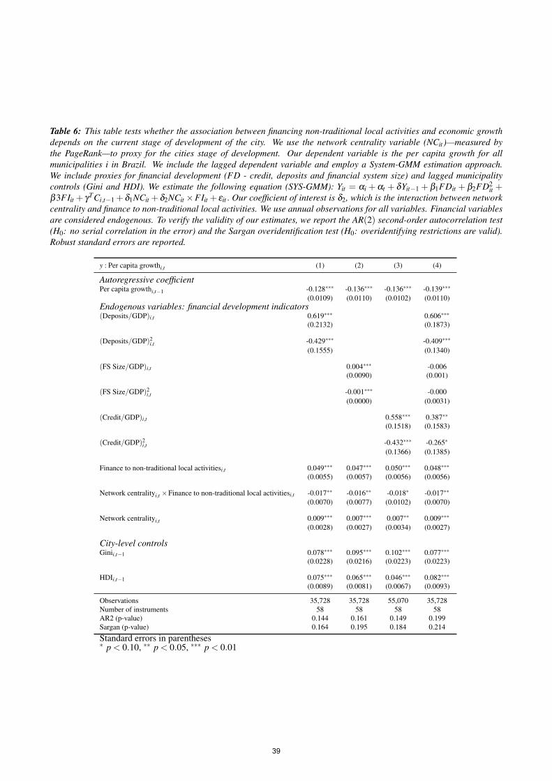
Table 6: This table tests whether the association between financing non-traditional local activities and economic growthdepends on the current stage of development of the city. We use the network centrality variable (NCit )—measured bythe PageRank—to proxy for the cities stage of development. Our dependent variable is the per capita growth for allmunicipalities i in Brazil. We include the lagged dependent variable and employ a System-GMM estimation approach.We include proxies for financial development (FD - credit, deposits and financial system size) and lagged municipalitycontrols (Gini and HDI). We estimate the following equation (SYS-GMM): Yit = αi +αt + δYit−1 + β1FDit + β2FD2
it +β3FIit + γTCi,t−1 +δ1NCit +δ2NCit ×FIit + εit . Our coefficient of interest is δ2, which is the interaction between networkcentrality and finance to non-traditional local activities. We use annual observations for all variables. Financial variablesare considered endogenous. To verify the validity of our estimates, we report the AR(2) second-order autocorrelation test(H0: no serial correlation in the error) and the Sargan overidentification test (H0: overidentifying restrictions are valid).Robust standard errors are reported.
y : Per capita growthi,t (1) (2) (3) (4)
Autoregressive coefficientPer capita growthi,t−1 -0.128∗∗∗ -0.136∗∗∗ -0.136∗∗∗ -0.139∗∗∗
(0.0109) (0.0110) (0.0102) (0.0110)Endogenous variables: financial development indicators(Deposits/GDP)i,t 0.619∗∗∗ 0.606∗∗∗
(0.2132) (0.1873)
(Deposits/GDP)2i,t -0.429∗∗∗ -0.409∗∗∗
(0.1555) (0.1340)
(FS Size/GDP)i,t 0.004∗∗∗ -0.006(0.0090) (0.001)
(FS Size/GDP)2i,t -0.001∗∗∗ -0.000
(0.0000) (0.0031)
(Credit/GDP)i,t 0.558∗∗∗ 0.387∗∗
(0.1518) (0.1583)
(Credit/GDP)2i,t -0.432∗∗∗ -0.265∗
(0.1366) (0.1385)
Finance to non-traditional local activitiesi,t 0.049∗∗∗ 0.047∗∗∗ 0.050∗∗∗ 0.048∗∗∗
(0.0055) (0.0057) (0.0056) (0.0056)
Network centralityi,t ×Finance to non-traditional local activitiesi,t -0.017∗∗ -0.016∗∗ -0.018∗ -0.017∗∗
(0.0070) (0.0077) (0.0102) (0.0070)
Network centralityi,t 0.009∗∗∗ 0.007∗∗∗ 0.007∗∗ 0.009∗∗∗
(0.0028) (0.0027) (0.0034) (0.0027)
City-level controlsGinii,t−1 0.078∗∗∗ 0.095∗∗∗ 0.102∗∗∗ 0.077∗∗∗
(0.0228) (0.0216) (0.0223) (0.0223)
HDIi,t−1 0.075∗∗∗ 0.065∗∗∗ 0.046∗∗∗ 0.082∗∗∗
(0.0089) (0.0081) (0.0067) (0.0093)
Observations 35,728 35,728 55,070 35,728Number of instruments 58 58 58 58AR2 (p-value) 0.144 0.161 0.149 0.199Sargan (p-value) 0.164 0.195 0.184 0.214
Standard errors in parentheses∗ p < 0.10, ∗∗ p < 0.05, ∗∗∗ p < 0.01
39
in cities at initial stages of development. This confirms our Hypothesis 5. Annex B shows a similaranalysis using the HDI as a proxy for city stage of development.
5.3 Spillovers and economic growth (Hypotheses 6–7)
We test whether municipalities that have neighbors at advanced stages of development (high central-ity) correlate positively with their own growth rates. Theoretically, there may be two main effects. Onthe one hand, if a municipality has a neighbor at a advanced stage of development, it may increaseits trading with it and boost its own economic growth. This would imply a positive spillover fromthe central region to the periphery. However, on the other hand, municipalities may be competing forresources and having central neighbors may impact negatively one’s own growth rate if the munici-palities loses resources to the central neighbors. This would generate a negative geographic spilloverbetween municipalities.
We also test whether there is economic spillover between municipalities. For each city i, we calculatethe weighted average centrality of all municipalities j that trade with i. The rationale of this measureis to capture the average stage of development of cities with which i transacts. If a municipality has alarge number of operations with municipalities with advanced stages of development, it may be seenas an important link in the production chain.
Table 7 reports our empirical results. We find that the own stage of development of the city (net-work centrality) correlates with economic growth with coefficients ranging from 2.8% to 3.3%. Eco-nomic spillovers respond with coefficients ranging from 1.8% to 2.2%, and geographic spillover with0.6% to 0.9%. The statistically significant and positive signs confirm our Hypotheses 6 and 7. Thestatistical strength of the economic spillover can be 2.1 to 3 times higher than that of geographicspillovers, whereas the municipality’s own stage of development is 1.5 to 1.8 times higher than eco-nomic spillovers, depending on the econometric specification.
We normalize the spillover variables and the network centrality to have zero mean and unitary standarddeviation (Z-score) to allow cross-comparisons. The results show that the municipality’s own stage ofdevelopment—measured by its network centrality—is the most relevant for economic growth, followedby economic and geographic spillovers, in this order. Nonetheless, the stage of development of the cityitself is the factor that correlates the strongest with its own growth rate. Our results suggest that beinginterconnected with other municipalities matters to economic growth.
5.4 Are financial development and activity diversification good for economicgrowth in times of distress? (Hypotheses 8–10)
A relevant question is whether financial development and finance to non-traditional local activitieshelp sustaining economic growth in times of distress. We use a natural disasters database to identifymunicipalities that have suffered from natural disasters and evaluate their per capita growth rates vis-a-vis similar but unaffected cities using a binary (existence of the shock) and continuous (extension of
40
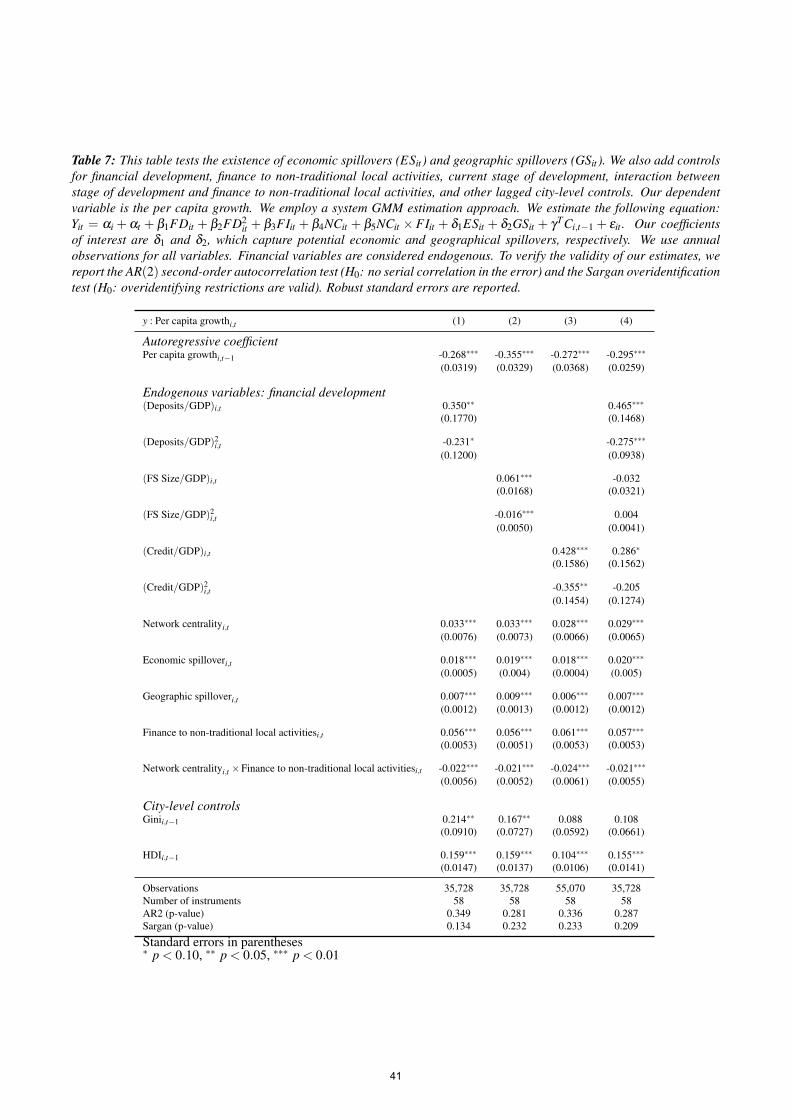
Table 7: This table tests the existence of economic spillovers (ESit ) and geographic spillovers (GSit ). We also add controlsfor financial development, finance to non-traditional local activities, current stage of development, interaction betweenstage of development and finance to non-traditional local activities, and other lagged city-level controls. Our dependentvariable is the per capita growth. We employ a system GMM estimation approach. We estimate the following equation:Yit = αi +αt + β1FDit + β2FD2
it + β3FIit + β4NCit + β5NCit × FIit + δ1ESit + δ2GSit + γTCi,t−1 + εit . Our coefficientsof interest are δ1 and δ2, which capture potential economic and geographical spillovers, respectively. We use annualobservations for all variables. Financial variables are considered endogenous. To verify the validity of our estimates, wereport the AR(2) second-order autocorrelation test (H0: no serial correlation in the error) and the Sargan overidentificationtest (H0: overidentifying restrictions are valid). Robust standard errors are reported.
y : Per capita growthi,t (1) (2) (3) (4)
Autoregressive coefficientPer capita growthi,t−1 -0.268∗∗∗ -0.355∗∗∗ -0.272∗∗∗ -0.295∗∗∗
(0.0319) (0.0329) (0.0368) (0.0259)
Endogenous variables: financial development(Deposits/GDP)i,t 0.350∗∗ 0.465∗∗∗
(0.1770) (0.1468)
(Deposits/GDP)2i,t -0.231∗ -0.275∗∗∗
(0.1200) (0.0938)
(FS Size/GDP)i,t 0.061∗∗∗ -0.032(0.0168) (0.0321)
(FS Size/GDP)2i,t -0.016∗∗∗ 0.004
(0.0050) (0.0041)
(Credit/GDP)i,t 0.428∗∗∗ 0.286∗
(0.1586) (0.1562)
(Credit/GDP)2i,t -0.355∗∗ -0.205
(0.1454) (0.1274)
Network centralityi,t 0.033∗∗∗ 0.033∗∗∗ 0.028∗∗∗ 0.029∗∗∗
(0.0076) (0.0073) (0.0066) (0.0065)
Economic spilloveri,t 0.018∗∗∗ 0.019∗∗∗ 0.018∗∗∗ 0.020∗∗∗
(0.0005) (0.004) (0.0004) (0.005)
Geographic spilloveri,t 0.007∗∗∗ 0.009∗∗∗ 0.006∗∗∗ 0.007∗∗∗
(0.0012) (0.0013) (0.0012) (0.0012)
Finance to non-traditional local activitiesi,t 0.056∗∗∗ 0.056∗∗∗ 0.061∗∗∗ 0.057∗∗∗
(0.0053) (0.0051) (0.0053) (0.0053)
Network centralityi,t ×Finance to non-traditional local activitiesi,t -0.022∗∗∗ -0.021∗∗∗ -0.024∗∗∗ -0.021∗∗∗
(0.0056) (0.0052) (0.0061) (0.0055)
City-level controlsGinii,t−1 0.214∗∗ 0.167∗∗ 0.088 0.108
(0.0910) (0.0727) (0.0592) (0.0661)
HDIi,t−1 0.159∗∗∗ 0.159∗∗∗ 0.104∗∗∗ 0.155∗∗∗
(0.0147) (0.0137) (0.0106) (0.0141)
Observations 35,728 35,728 55,070 35,728Number of instruments 58 58 58 58AR2 (p-value) 0.349 0.281 0.336 0.287Sargan (p-value) 0.134 0.232 0.233 0.209
Standard errors in parentheses∗ p < 0.10, ∗∗ p < 0.05, ∗∗∗ p < 0.01
41
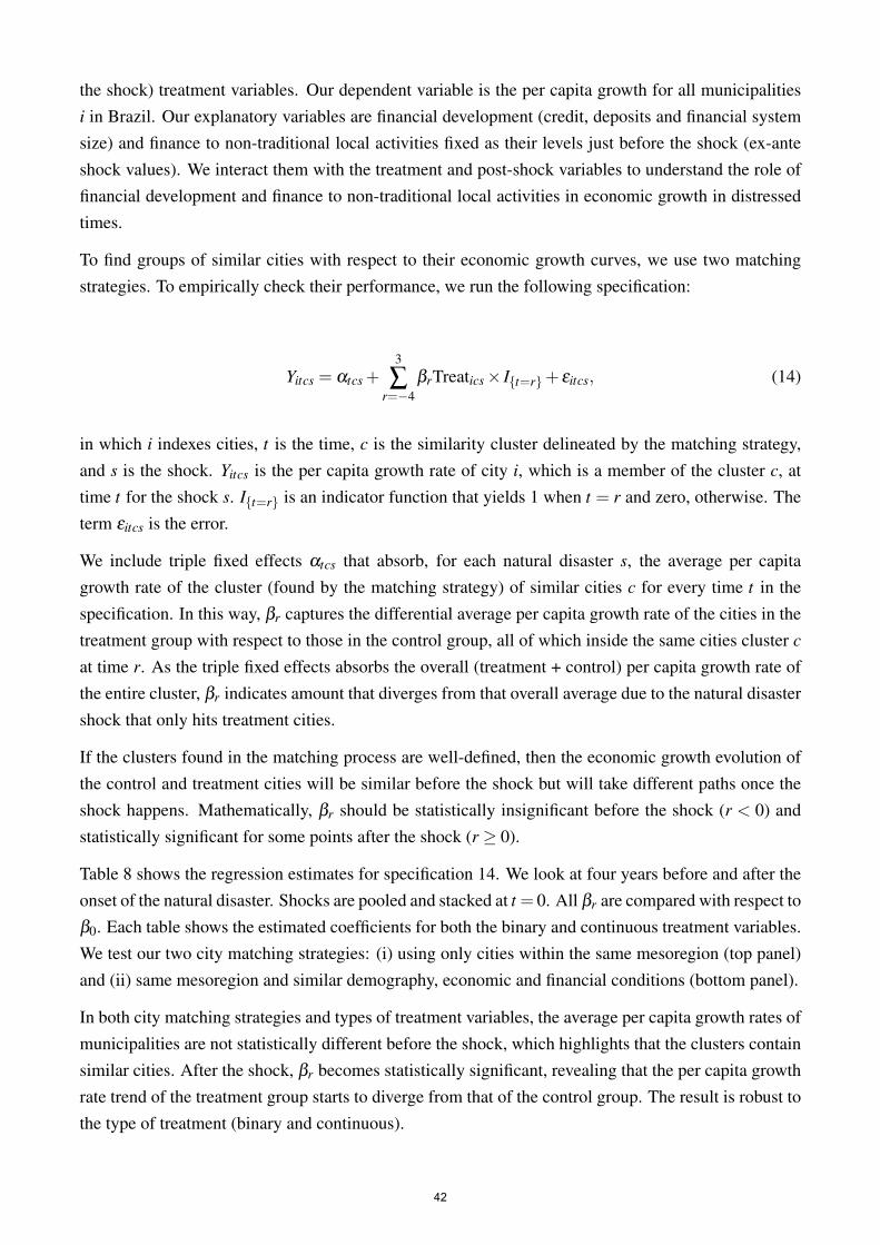
the shock) treatment variables. Our dependent variable is the per capita growth for all municipalitiesi in Brazil. Our explanatory variables are financial development (credit, deposits and financial systemsize) and finance to non-traditional local activities fixed as their levels just before the shock (ex-anteshock values). We interact them with the treatment and post-shock variables to understand the role offinancial development and finance to non-traditional local activities in economic growth in distressedtimes.
To find groups of similar cities with respect to their economic growth curves, we use two matchingstrategies. To empirically check their performance, we run the following specification:
Yitcs = αtcs +3
∑r=−4
βrTreatics× I{t=r}+ εitcs, (14)
in which i indexes cities, t is the time, c is the similarity cluster delineated by the matching strategy,and s is the shock. Yitcs is the per capita growth rate of city i, which is a member of the cluster c, attime t for the shock s. I{t=r} is an indicator function that yields 1 when t = r and zero, otherwise. Theterm εitcs is the error.
We include triple fixed effects αtcs that absorb, for each natural disaster s, the average per capitagrowth rate of the cluster (found by the matching strategy) of similar cities c for every time t in thespecification. In this way, βr captures the differential average per capita growth rate of the cities in thetreatment group with respect to those in the control group, all of which inside the same cities cluster c
at time r. As the triple fixed effects absorbs the overall (treatment + control) per capita growth rate ofthe entire cluster, βr indicates amount that diverges from that overall average due to the natural disastershock that only hits treatment cities.
If the clusters found in the matching process are well-defined, then the economic growth evolution ofthe control and treatment cities will be similar before the shock but will take different paths once theshock happens. Mathematically, βr should be statistically insignificant before the shock (r < 0) andstatistically significant for some points after the shock (r ≥ 0).
Table 8 shows the regression estimates for specification 14. We look at four years before and after theonset of the natural disaster. Shocks are pooled and stacked at t = 0. All βr are compared with respect toβ0. Each table shows the estimated coefficients for both the binary and continuous treatment variables.We test our two city matching strategies: (i) using only cities within the same mesoregion (top panel)and (ii) same mesoregion and similar demography, economic and financial conditions (bottom panel).
In both city matching strategies and types of treatment variables, the average per capita growth rates ofmunicipalities are not statistically different before the shock, which highlights that the clusters containsimilar cities. After the shock, βr becomes statistically significant, revealing that the per capita growthrate trend of the treatment group starts to diverge from that of the control group. The result is robust tothe type of treatment (binary and continuous).
42
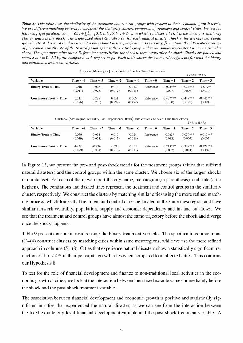
Table 8: This table tests the similarity of the treatment and control groups with respect to their economic growth levels.We use different matching criteria to construct the similarity clusters composed of treatment and control cities. We test thefollowing specification: Yitcs = αtcs +∑
3r=−4 βrTreatics× It=r + εitcs, in which i indexes cities, t is the time, c is similarity
cluster, and s is the shock. The triple fixed effect αtcs absorbs, for each natural disaster shock s, the average per capitagrowth rate of cluster of similar cities c for every time t in the specification. In this way, βr captures the differential averageof per capita growth rate of the treated group against the control group within the similarity cluster for each particularshock. The uppermost table shows βr from four years before the shock to three years after the shock. Shocks are pooled andstacked at t = 0. All βr are compared with respect to β0. Each table shows the estimated coefficients for both the binaryand continuous treatment variable.
Cluster = {Mesoregion} with cluster x Shock x Time fixed effects# obs = 10,457
Variable Time = -4 Time = -3 Time = -2 Time = -1 Time = 0 Time = 1 Time = 2 Time = 3
Binary Treat × Time 0.016 0.026 0.014 0.012 Reference -0.026*** -0.024*** -0.019**(0.017) (0.023) (0.012) (0.011) (0.007) (0.009) (0.010)
Continuous Treat × Time 0.211 0.287 0.351 0.506 Reference -0.437*** -0.447*** -0.546***(0.176) (0.230) (0.299) (0.479) (0.160) (0.191) (0.191)
Cluster = {Mesoregion, centrality, Gini, dependence, flows} with cluster x Shock x Time fixed effects# obs = 6,512
Variable Time = -4 Time = -3 Time = -2 Time = -1 Time = 0 Time = 1 Time = 2 Time = 3
Binary Treat × Time 0.030 0.031 0.019 0.024 Reference -0.023* -0.029*** -0.017***(0.019) (0.021) (0.015) (0.016) (0.012) (0.007) (0.005)
Continuous Treat × Time -0.090 -0.236 -0.241 -0.125 Reference -0.213*** -0.348*** -0.322***(0.829) (0.834) (0.810) (0.817) (0.057) (0.084) (0.102)
In Figure 13, we present the pre- and post-shock trends for the treatment groups (cities that sufferednatural disasters) and the control groups within the same cluster. We choose six of the largest shocksin our dataset. For each of them, we report the city name, mesoregion (in parenthesis), and state (afterhyphen). The continuous and dashed lines represent the treatment and control groups in the similaritycluster, respectively. We construct the clusters by matching similar cities using the more refined match-ing process, which forces that treatment and control cities be located in the same mesoregion and havesimilar network centrality, population, supply and customer dependency and in- and out-flows. Wesee that the treatment and control groups have almost the same trajectory before the shock and divergeonce the shock happens.
Table 9 presents our main results using the binary treatment variable. The specifications in columns(1)–(4) construct clusters by matching cities within same mesoregions, while we use the more refinedapproach in columns (5)–(8). Cities that experience natural disasters show a statistically significant re-duction of 1.5–2.4% in their per capita growth rates when compared to unaffected cities. This confirmsour Hypothesis 8.
To test for the role of financial development and finance to non-traditional local activities in the eco-nomic growth of cities, we look at the interaction between their fixed ex-ante values immediately beforethe shock and the post-shock treatment variable.
The association between financial development and economic growth is positive and statistically sig-nificant in cities that experienced the natural disaster, as we can see from the interaction betweenthe fixed ex-ante city-level financial development variable and the post-shock treatment variable. A
43
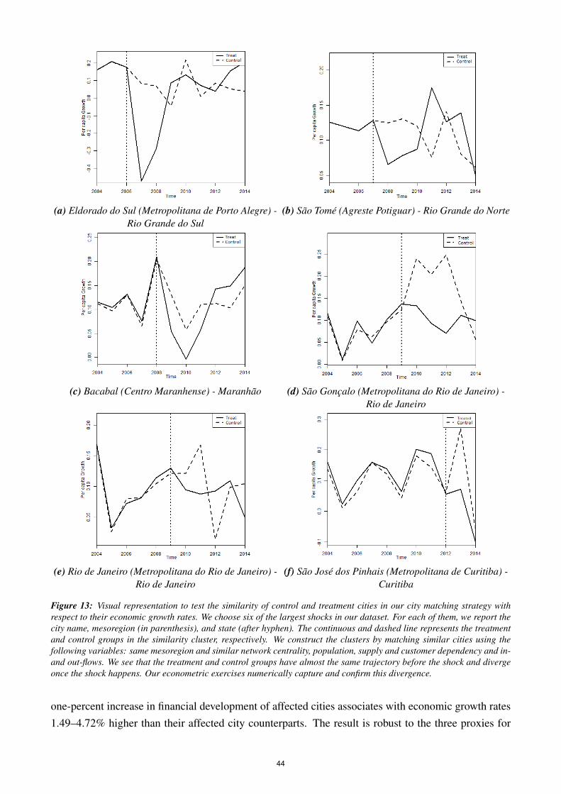
(a) Eldorado do Sul (Metropolitana de Porto Alegre) -Rio Grande do Sul
(b) Sao Tome (Agreste Potiguar) - Rio Grande do Norte
(c) Bacabal (Centro Maranhense) - Maranhao (d) Sao Goncalo (Metropolitana do Rio de Janeiro) -Rio de Janeiro
(e) Rio de Janeiro (Metropolitana do Rio de Janeiro) -Rio de Janeiro
(f) Sao Jose dos Pinhais (Metropolitana de Curitiba) -Curitiba
Figure 13: Visual representation to test the similarity of control and treatment cities in our city matching strategy withrespect to their economic growth rates. We choose six of the largest shocks in our dataset. For each of them, we report thecity name, mesoregion (in parenthesis), and state (after hyphen). The continuous and dashed line represents the treatmentand control groups in the similarity cluster, respectively. We construct the clusters by matching similar cities using thefollowing variables: same mesoregion and similar network centrality, population, supply and customer dependency and in-and out-flows. We see that the treatment and control groups have almost the same trajectory before the shock and divergeonce the shock happens. Our econometric exercises numerically capture and confirm this divergence.
one-percent increase in financial development of affected cities associates with economic growth rates1.49–4.72% higher than their affected city counterparts. The result is robust to the three proxies for
44
financial development: deposits (columns 2 and 6), financial system size (columns 3 and 7), and credit(columns 4 and 8). These results confirm Hypothesis 9.
It is important to note that the non-linearity between financial development and economic growth innormal times does not prevail when cities are experiencing times of distress. We observe that onlythe linear coefficient of financial development remains statistically significant. In this case, more bankcredit associates with higher economic growth rates. This may be due to the fact that, in distressedsituations, residents may need extra cash to recover from their losses.
In contrast, cities in which banks finance more non-traditional local activities relatively to their tradi-tional activities suffer more from natural disasters. A one-percent increase in finance to non-traditionallocal activities (activity diversification) in affected cities is associated with 2.3–5.6% lower economicgrowth rates. This result is robust to both city matching strategies. These results confirm Hypothesis10.
In Table 10, we present the results of our differences-in-differences approach using the continuoustreatment variable. Cities that experience natural disasters show a reduction of 7.2-13.5% of their percapita growth rates relatively to unaffected similar cities. Our estimates using the continuous treatmentvariable are higher than those using the binary version. One explanation is that the distribution oflosses of natural disasters decreases very rapidly. In this way, few cities are heavily affected whileothers are not, even in the case when are looking at the largest shocks over the period of 2004-2014 inBrazil. The continuous variable is able to bring this heterogeneity into the regression estimates, whilethe binary version cannot. In the last, every affected city is treated homogeneously.
We also find that the interaction between treatment, post-shock and ex-ante finance to non-traditionallocal activities has a negative signal and is statistically significant for almost all specifications in whichwe use different proxies for financial development. Only in the case of the use of deposits and forsecond matching strategy (mesoregion, centrality, Gini, dependence and flows) this interaction is notstatistically significant. The results suggest that after adverse shocks from natural disasters, financingfor ex-ante non-traditional local activities associates with lower economic growth rates.
By looking at the triple interaction between treatment, post-shock and ex-ante financial development,we see that the linear coefficient remains statistically significant and positive for all financial develop-ment proxies in the two different matching strategies. However, the triple interaction using the squareof ex-ante financial development is not statistically significant. This result corroborates our previousfindings with the binary treatment variable.
6 Conclusion
The paper finds a series of results that contribute to the link between financial development and eco-nomic growth. We find that financial development helps explain economic growth by using an ex-tremely rich and detailed database for Brazilian municipalities. We find that there is a non-linearassociation between financial development and growth during normal times. This suggests that, af-
45
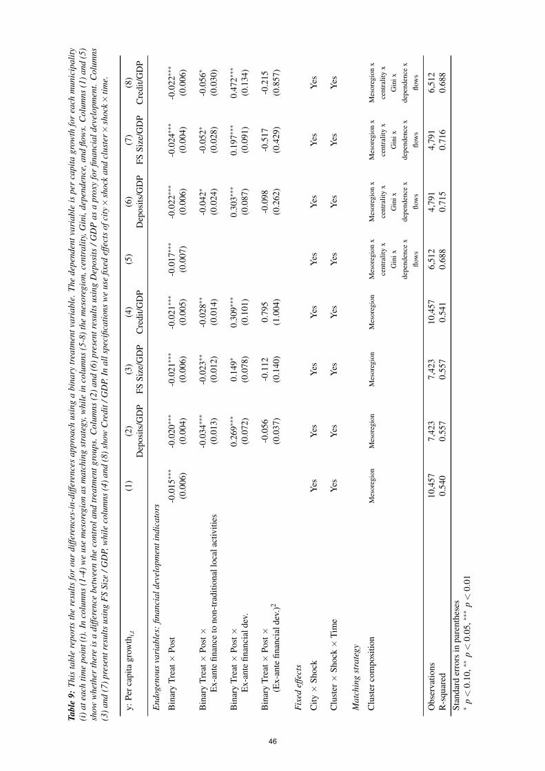
T abl
e9:
This
tabl
ere
port
sth
ere
sults
for
our
diffe
renc
es-i
n-di
ffere
nces
appr
oach
usin
ga
bina
rytr
eatm
entv
aria
ble.
The
depe
nden
tvar
iabl
eis
per
capi
tagr
owth
for
each
mun
icip
ality
(i)a
teac
htim
epo
int(
t).I
nco
lum
ns(1
-4)w
eus
em
esor
egio
nas
mat
chin
gst
rate
gy,w
hile
inco
lum
ns(5
-8)t
hem
esor
egio
n,ce
ntra
lity,
Gin
i,de
pend
ence
,and
flow
s.C
olum
ns(1
)and
(5)
show
whe
ther
ther
eis
adi
ffere
nce
betw
een
the
cont
rola
ndtr
eatm
entg
roup
s.C
olum
ns(2
)an
d(6
)pr
esen
tres
ults
usin
gD
epos
its/G
DP
asa
prox
yfo
rfin
anci
alde
velo
pmen
t.C
olum
ns(3
)and
(7)p
rese
ntre
sults
usin
gF
SSi
ze/G
DP,
whi
leco
lum
ns(4
)and
(8)s
how
Cre
dit/
GD
P.In
alls
peci
ficat
ions
we
use
fixed
effe
cts
ofci
ty×
shoc
kan
dcl
uste
r×sh
ock×
time.
y:Pe
rcap
itagr
owth
i,t(1
)(2
)(3
)(4
)(5
)(6
)(7
)(8
)D
epos
its/G
DP
FSSi
ze/G
DP
Cre
dit/G
DP
Dep
osits
/GD
PFS
Size
/GD
PC
redi
t/GD
P
End
ogen
ous
vari
able
s:fin
anci
alde
velo
pmen
tind
icat
ors
Bin
ary
Trea
t×Po
st-0
.015∗∗∗
-0.0
20∗∗∗
-0.0
21∗∗∗
-0.0
21∗∗∗
-0.0
17∗∗∗
-0.0
22∗∗∗
-0.0
24∗∗∗
-0.0
22∗∗∗
(0.0
06)
(0.0
04)
(0.0
06)
(0.0
05)
(0.0
07)
(0.0
06)
(0.0
04)
(0.0
06)
Bin
ary
Trea
t×Po
st×
-0.0
34∗∗∗
-0.0
23∗∗
-0.0
28∗∗
-0.0
42∗
-0.0
52∗
-0.0
56∗
Ex-
ante
finan
ceto
non-
trad
ition
allo
cala
ctiv
ities
(0.0
13)
(0.0
12)
(0.0
14)
(0.0
24)
(0.0
28)
(0.0
30)
Bin
ary
Trea
t×Po
st×
0.26
9∗∗∗
0.14
9∗0.
309∗∗∗
0.30
3∗∗∗
0.19
7∗∗∗
0.47
2∗∗∗
Ex-
ante
finan
cial
dev.
(0.0
72)
(0.0
78)
(0.1
01)
(0.0
87)
(0.0
91)
(0.1
34)
Bin
ary
Trea
t×Po
st×
-0.0
56-0
.112
0.79
5-0
.098
-0.5
17-0
.215
(Ex-
ante
finan
cial
dev.
)2(0
.037
)(0
.140
)(1
.004
)(0
.262
)(0
.429
)(0
.857
)
Fixe
def
fect
s
City×
Shoc
kY
esY
esY
esY
esY
esY
esY
esY
es
Clu
ster×
Shoc
k×
Tim
eY
esY
esY
esY
esY
esY
esY
esY
es
Mat
chin
gst
rate
gy
Clu
ster
com
posi
tion
Mes
oreg
ion
Mes
oreg
ion
Mes
oreg
ion
Mes
oreg
ion
Mes
oreg
ion
xM
esor
egio
nx
Mes
oreg
ion
xM
esor
egio
nx
cent
ralit
yx
cent
ralit
yx
cent
ralit
yx
cent
ralit
yx
Gin
ixG
inix
Gin
ixG
inix
depe
nden
cex
depe
nden
cex
depe
nden
cex
depe
nden
cex
flow
sflo
ws
flow
sflo
ws
Obs
erva
tions
10,4
577,
423
7,42
310
,457
6,51
24,
791
4,79
16,
512
R-s
quar
ed0.
540
0.55
70.
557
0.54
10.
688
0.71
50.
716
0.68
8St
anda
rder
rors
inpa
rent
hese
s∗
p<
0.10
,∗∗
p<
0.05
,∗∗∗
p<
0.01
46
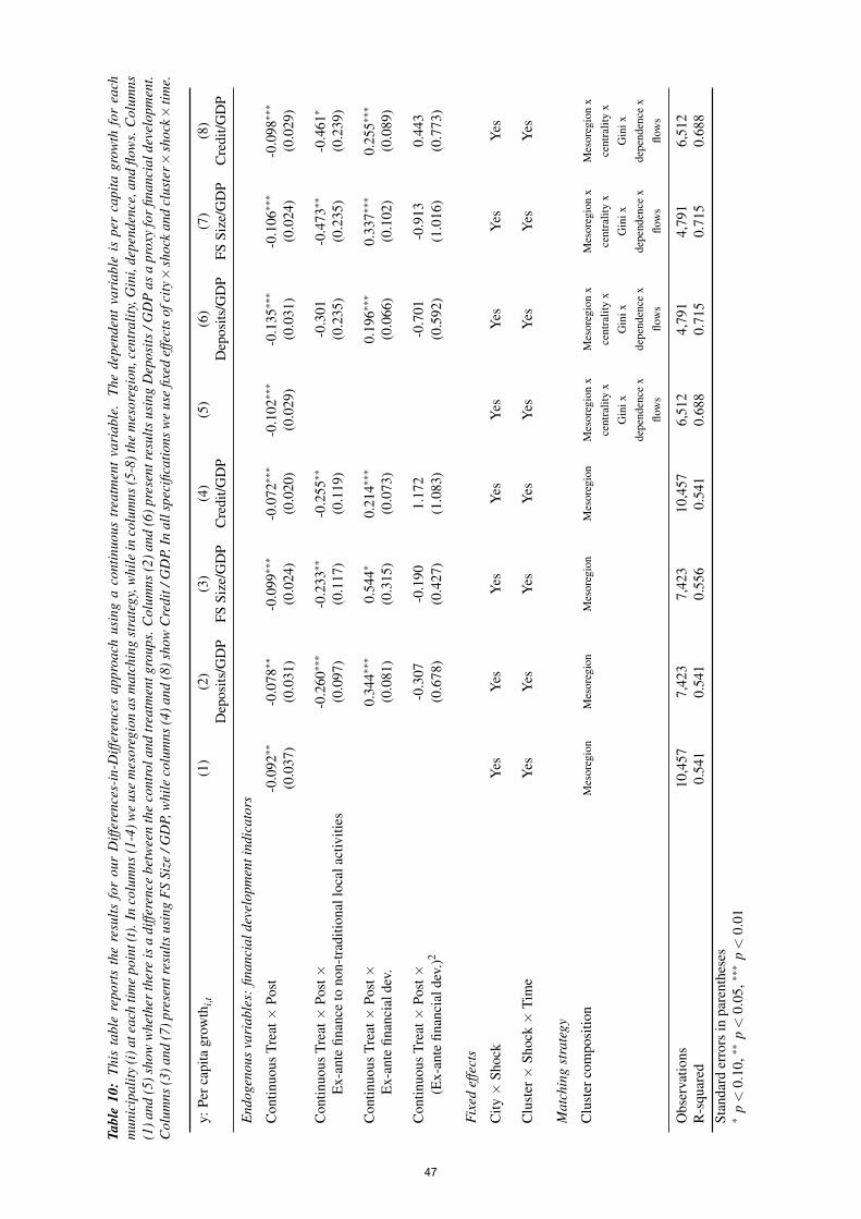
T abl
e10
:Th
ista
ble
repo
rts
the
resu
ltsfo
rou
rD
iffer
ence
s-in
-Diff
eren
ces
appr
oach
usin
ga
cont
inuo
ustr
eatm
ent
vari
able
.Th
ede
pend
ent
vari
able
ispe
rca
pita
grow
thfo
rea
chm
unic
ipal
ity(i
)ate
ach
time
poin
t(t)
.In
colu
mns
(1-4
)we
use
mes
oreg
ion
asm
atch
ing
stra
tegy
,whi
lein
colu
mns
(5-8
)the
mes
oreg
ion,
cent
ralit
y,G
ini,
depe
nden
ce,a
ndflo
ws.
Col
umns
(1)a
nd(5
)sho
ww
heth
erth
ere
isa
diffe
renc
ebe
twee
nth
eco
ntro
land
trea
tmen
tgro
ups.
Col
umns
(2)a
nd(6
)pre
sent
resu
ltsus
ing
Dep
osits
/GD
Pas
apr
oxy
for
finan
cial
deve
lopm
ent.
Col
umns
(3)a
nd(7
)pre
sent
resu
ltsus
ing
FS
Size
/GD
P,w
hile
colu
mns
(4)a
nd(8
)sho
wC
redi
t/G
DP.
Inal
lspe
cific
atio
nsw
eus
efix
edef
fect
sof
city×
shoc
kan
dcl
uste
r×sh
ock×
time.
y:Pe
rcap
itagr
owth
i,t(1
)(2
)(3
)(4
)(5
)(6
)(7
)(8
)D
epos
its/G
DP
FSSi
ze/G
DP
Cre
dit/G
DP
Dep
osits
/GD
PFS
Size
/GD
PC
redi
t/GD
P
End
ogen
ous
vari
able
s:fin
anci
alde
velo
pmen
tind
icat
ors
Con
tinuo
usTr
eat×
Post
-0.0
92∗∗
-0.0
78∗∗
-0.0
99∗∗∗
-0.0
72∗∗∗
-0.1
02∗∗∗
-0.1
35∗∗∗
-0.1
06∗∗∗
-0.0
98∗∗∗
(0.0
37)
(0.0
31)
(0.0
24)
(0.0
20)
(0.0
29)
(0.0
31)
(0.0
24)
(0.0
29)
Con
tinuo
usTr
eat×
Post×
-0.2
60∗∗∗
-0.2
33∗∗
-0.2
55∗∗
-0.3
01-0
.473∗∗
-0.4
61∗
Ex-
ante
finan
ceto
non-
trad
ition
allo
cala
ctiv
ities
(0.0
97)
(0.1
17)
(0.1
19)
(0.2
35)
(0.2
35)
(0.2
39)
Con
tinuo
usTr
eat×
Post×
0.34
4∗∗∗
0.54
4∗0.
214∗∗∗
0.19
6∗∗∗
0.33
7∗∗∗
0.25
5∗∗∗
Ex-
ante
finan
cial
dev.
(0.0
81)
(0.3
15)
(0.0
73)
(0.0
66)
(0.1
02)
(0.0
89)
Con
tinuo
usTr
eat×
Post×
-0.3
07-0
.190
1.17
2-0
.701
-0.9
130.
443
(Ex-
ante
finan
cial
dev.
)2(0
.678
)(0
.427
)(1
.083
)(0
.592
)(1
.016
)(0
.773
)
Fixe
def
fect
s
City×
Shoc
kY
esY
esY
esY
esY
esY
esY
esY
es
Clu
ster×
Shoc
k×
Tim
eY
esY
esY
esY
esY
esY
esY
esY
es
Mat
chin
gst
rate
gy
Clu
ster
com
posi
tion
Mes
oreg
ion
Mes
oreg
ion
Mes
oreg
ion
Mes
oreg
ion
Mes
oreg
ion
xM
esor
egio
nx
Mes
oreg
ion
xM
esor
egio
nx
cent
ralit
yx
cent
ralit
yx
cent
ralit
yx
cent
ralit
yx
Gin
ixG
inix
Gin
ixG
inix
depe
nden
cex
depe
nden
cex
depe
nden
cex
depe
nden
cex
flow
sflo
ws
flow
sflo
ws
Obs
erva
tions
10,4
577,
423
7,42
310
,457
6,51
24,
791
4,79
16,
512
R-s
quar
ed0.
541
0.54
10.
556
0.54
10.
688
0.71
50.
715
0.68
8St
anda
rder
rors
inpa
rent
hese
s∗
p<
0.10
,∗∗
p<
0.05
,∗∗∗
p<
0.01
47
ter a certain stage of financial development, the partial correlation between financial development andeconomic growth becomes negative.
We develop a new city-level measure of finance to non-traditional local activities that proves to beimportant in explaining economic growth. This measure can be conceived as a proxy for local activitydiversification. Municipalities where banks finance more strongly non-traditional local activities areassociated with higher economic growth rates. This finding is important since it shows that who getscredit (borrower side) is also important for economic growth.
Using measures of complex networks theory, we create spillover measures among municipalities andshow that they are relevant for economic growth. To test for geographical spillovers, we inspectwhether cities nearby advanced centers have higher economic rates. Analogously, we look at eco-nomic spillovers by checking whether transacting with cities at advanced stages of development as-sociate more strongly with economic growth. From an economic perspective, we find that economicspillover correlates more with growth than geographic spillover.
We analyze the firm-to-firm trade network for all Brazilian municipalities and find that this network hasa core-periphery structure, in which there are few municipalities—the core—that are highly connectto a large number of other municipalities—the periphery. In addition, it presents disassortative mixingand small network diameter, suggesting that city hubs are important for economically bridging smallcities far apart. We then use this rich network structure to estimate the current stage of development ofeach city in Brazil. We use the PageRank network centrality to proxy for cities stages of development,which takes into account not only the quantity of connections of a city, but also their quality.
We use natural disasters to analyze the relationships between economic growth, financial development,and bank financing to non-traditional local activities in times of distress. Our results show that thetraditional non-linear relationship found in the finance-growth literature between financial developmentand economic growth breaks down when cities are suffering from adverse shocks. In times of distress,the association of financial development and economic growth is positive is regardless of the currentlevels of financial development within the city. In addition, financing non-traditional activities becomesnegatively associated with economic growth during times of distress. This suggests that municipalitiesexperiencing natural disasters are better off when they focus on financing more fiercely their traditionalactivities rather than diversifying activities by financing non-traditional local activities.
References
Abedifar, P., Hasan, I., and Tarazi, A. (2016). Finance-growth nexus and dual-banking systems: Rela-tive importance of Islamic banks. Journal of Economic Behavior and Organization, 132:198–215.
Andersson, F. N. G., Burzynska, K., and Opper, S. (2016). Lending for growth? A Granger causalityanalysis of China’s finance-growth nexus. EMPIRICAL ECONOMICS, 51(3):897–920.
Arellano, M. and Bover, O. (1995). Another look at the instrumental-variable estimation of error-components models. Journal of Econometrics, 68:29–52.
48
Beck, R., Georgiadis, G., and Straub, R. (2014a). The finance and growth nexus revisited. Economics
Letters, 124:382–385.
Beck, T., Degryse, H., and Kneer, C. (2014b). Is more finance better? Disentangling intermediationand size effects of financial systems. Journal of Financial Stability, 10:50–64.
Beck, T. and Levine, R. (2004). Stock markets, banks, and growth: Panel evidence. Journal of Banking
and Finance, 28:423–442.
Beck, T., Levine, R., and Loayza, N. (2000). Finance and the sources of growth. Journal of Financial
Economics, 58(1-2):261–300.
Beck, T., Lu, L., and Yang, R. (2015). Finance and growth for microenterprises: Evidence from ruralChina. World Development, 67:38–56.
Blundell, R. and Bond, S. (1998). Initial conditions and moment restrictions in dynamic panel datamodels. Journal of Econometrics, 87:115–143.
Blundell, R. and Bond, S. (2000). GMM estimation with persistent panel data: an application toproduction functions. Econometric Reviews, 19(3):321–340.
Debortoli, N. S., Camarinha, P. I. M., Marengo, J. A., and Rodrigues, R. R. (2017). An index ofBrazil’s vulnerability to expected increases in natural flash flooding and landslide disasters in thecontext of climate change. Natural Hazards, 86(2):557–582.
El-Khatib, R., Fogel, K., and Jandik, T. (2015). CEO network centrality and merger performance.Journal of Financial Economics, 116(2):349–82.
Freire, C. (2019). Economic diversification: A model of structural economic dynamics and endogenoustechnological change. Structural Change and Economic Dynamics, 49:13 – 28.
Haddad, E. A. and Teixeira, E. (2015). Economic impacts of natural disasters in megacities: The caseof floods in Sao Paulo, brazil. Habitat International, 45:106 – 113.
Herwartz, H. and Walle, Y. M. (2014). Openness and the finance-growth nexus. Journal of Banking
Finance, 48:235 – 247.
Jayaratne, J. and Strahan, P. E. (1996). The finance-growth nexus: Evidence from bank branch dereg-ulation. The Quarterly Journal of Economics, 111(3):639–670.
Kendall, J. (2012). Local financial development and growth. Journal of Banking & Finance,36(5):1548–1562.
King, R. G. and Levine, R. (1993). Finance and growth: Schumpeter might be right. The Quarterly
Journal of Economics, 108(3):717–737.
Konstantakopoulou, I. and Tsionas, M. G. (2019). Measuring comparative advantages in the euro area.Economic Modelling, 76:260 – 269.
49
Law, S. H., Azman-Saini, W., and Ibrahim, M. H. (2013). Institutional quality thresholds and thefinance–growth nexus. Journal of Banking & Finance, 37(12):5373–5381.
Law, S. H. and Singh, N. (2014). Does too much finance harm economic growth? Journal of Banking
and Finance, 41:36–44.
Levine, R. (2005). Finance and growth: Theory and evidence. Handbook of Economic Growth, 1(PartA):865–934.
Levine, R. and Zervos, S. (1998). Stock markets, banks, and economic growth. American Economic
Review, 88(3):537–558.
Morganti, P. and Garofalo, G. (2019). Reassessing the law, finance, and growth nexus after the recentgreat recession. Journal of Economic Behavior Organization, 162:229 – 250.
Rajan, R. and Zingales, L. (1998). Financial dependence and growth. American Economic Review,88(3):559–586.
Rajan, R. G. (2006). Has finance made the world riskier? European Financial Management,12(4):499–533.
Rioja, F. and Valev, N. (2004). Does one size fit all? A reexamination of the finance and growthrelationship. Journal of Development Economics, 74(2):429–447.
Rossi, A. G., Blake, D., Timmermann, A., Tonks, I., and Wermers, R. (2018). Network centrality anddelegated investment performance. Journal of Financial Economics, 128(1):183–206.
Rousseau, P. L. and Wachtel, P. (2002). Inflation thresholds and the finance–growth nexus. Journal of
International Money and Finance, 21(6):777 – 793. International Financial Integration.
Samargandi, N., Fidrmuc, J., and Ghosh, S. (2015). Is the relationship between financial developmentand economic growth monotonic? Evidence from a sample of middle-income countries. World
Development, 68:66 – 81.
Silva, T. C., de Souza, S. R. S., and Tabak, B. M. (2016a). Network structure analysis of the Brazilianinterbank market. Emerging Markets Review, 26:130 – 152.
Silva, T. C., Guerra, S. M., Tabak, B. M., and de Castro Miranda, R. C. (2016b). Financial networks,bank efficiency and risk-taking. Journal of Financial Stability, 25:247–257.
Silva, T. C. and Zhao, L. (2016). Machine Learning in Complex Networks. Springer.
Slesman, L., Baharumshah, A. Z., and Azman-Saini, W. (2019). Political institutions and finance-growth nexus in emerging markets and developing countries: A tale of one threshold. The Quarterly
Review of Economics and Finance, 72:80–100.
Soedarmono, W., Hasan, I., and Arsyad, N. (2017). Non-linearity in the finance-growth nexus: Evi-dence from Indonesia? International Economics, 150:19–35.
Tobin, J. (1984). On the efficiency of the financial system. Lloyds Bank Rev., 153:1–15.
50
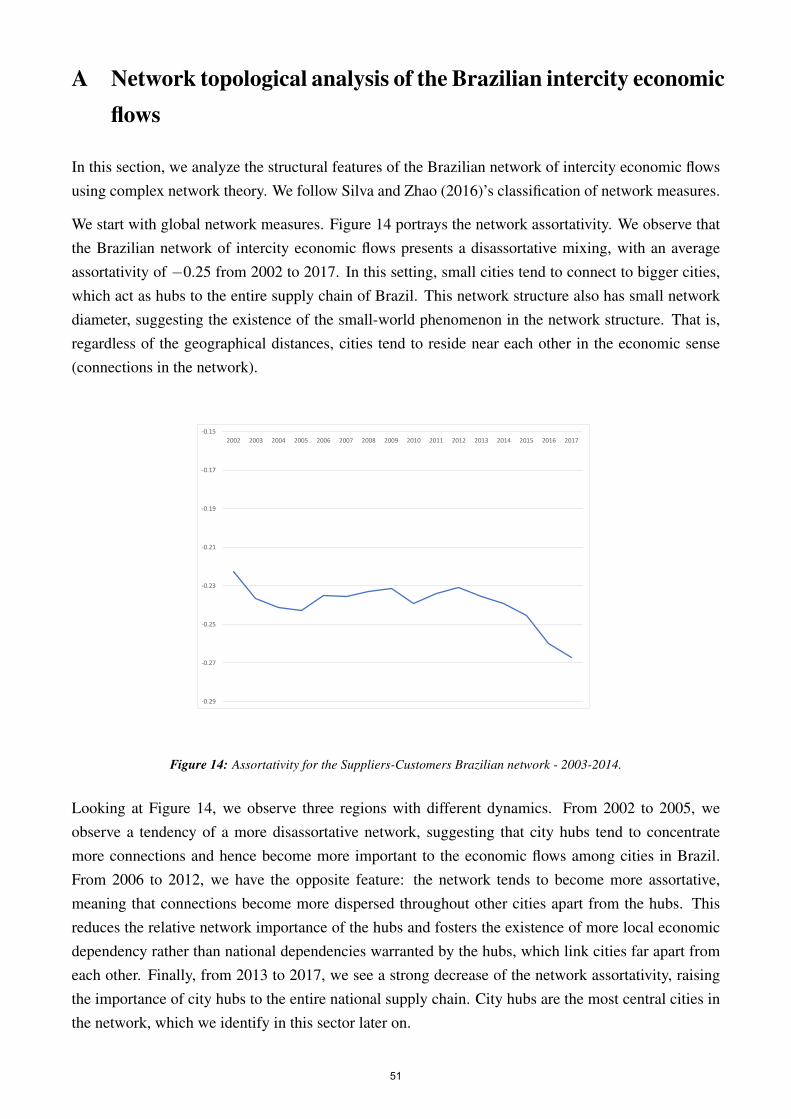
A Network topological analysis of the Brazilian intercity economicflows
In this section, we analyze the structural features of the Brazilian network of intercity economic flowsusing complex network theory. We follow Silva and Zhao (2016)’s classification of network measures.
We start with global network measures. Figure 14 portrays the network assortativity. We observe thatthe Brazilian network of intercity economic flows presents a disassortative mixing, with an averageassortativity of −0.25 from 2002 to 2017. In this setting, small cities tend to connect to bigger cities,which act as hubs to the entire supply chain of Brazil. This network structure also has small networkdiameter, suggesting the existence of the small-world phenomenon in the network structure. That is,regardless of the geographical distances, cities tend to reside near each other in the economic sense(connections in the network).
-0.29
-0.27
-0.25
-0.23
-0.21
-0.19
-0.17
-0.15
2002 2003 2004 2005 2006 2007 2008 2009 2010 2011 2012 2013 2014 2015 2016 2017
Figure 14: Assortativity for the Suppliers-Customers Brazilian network - 2003-2014.
Looking at Figure 14, we observe three regions with different dynamics. From 2002 to 2005, weobserve a tendency of a more disassortative network, suggesting that city hubs tend to concentratemore connections and hence become more important to the economic flows among cities in Brazil.From 2006 to 2012, we have the opposite feature: the network tends to become more assortative,meaning that connections become more dispersed throughout other cities apart from the hubs. Thisreduces the relative network importance of the hubs and fosters the existence of more local economicdependency rather than national dependencies warranted by the hubs, which link cities far apart fromeach other. Finally, from 2013 to 2017, we see a strong decrease of the network assortativity, raisingthe importance of city hubs to the entire national supply chain. City hubs are the most central cities inthe network, which we identify in this sector later on.
51
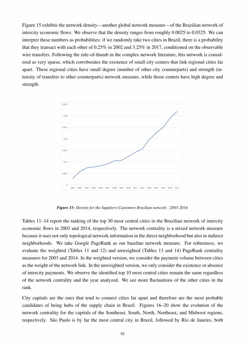
Figure 15 exhibits the network density—another global network measure—of the Brazilian network ofintercity economic flows. We observe that the density ranges from roughly 0.0025 to 0.0325. We caninterpret these numbers as probabilities: if we randomly take two cities in Brazil, there is a probabilitythat they transact with each other of 0.25% in 2002 and 3.25% in 2017, conditioned on the observablewire transfers. Following the rule-of-thumb in the complex network literature, this network is consid-ered as very sparse, which corroborates the existence of small city centers that link regional cities farapart. These regional cities have small degree (number of other city counterparts) and strength (in-tensity of transfers to other counterparts) network measure, while those centers have high degree andstrength.
0
0.005
0.01
0.015
0.02
0.025
0.03
0.035
2002 2003 2004 2005 2006 2007 2008 2009 2010 2011 2012 2013 2014 2015 2016 2017
Figure 15: Density for the Suppliers-Customers Brazilian network - 2003-2014.
Tables 11–14 report the ranking of the top 30 most central cities in the Brazilian network of intercityeconomic flows in 2003 and 2014, respectively. The network centrality is a mixed network measurebecause it uses not only topological network information in the direct neighborhood but also in indirectneighborhoods. We take Google PageRank as our baseline network measure. For robustness, weevaluate the weighted (Tables 11 and 12) and unweighted (Tables 13 and 14) PageRank centralitymeasures for 2003 and 2014. In the weighted version, we consider the payment volume between citiesas the weight of the network link. In the unweighted version, we only consider the existence or absenceof intercity payments. We observe the identified top 10 most central cities remain the same regardlessof the network centrality and the year analyzed. We see more fluctuations of the other cities in therank.
City capitals are the ones that tend to connect cities far apart and therefore are the most probablecandidates of being hubs of the supply chain in Brazil. Figures 16–20 show the evolution of thenetwork centrality for the capitals of the Southeast, South, North, Northeast, and Midwest regions,respectively. Sao Paulo is by far the most central city in Brazil, followed by Rio de Janeiro, both
52

Table 11: This Table presents the Ranking of 30 Municipalities with the largest Centrality for the year 2003.
Ranking Centrality Municipality State Region1 0.218932372 Sao Paulo Sao Paulo Southeast2 0.159346025 Rio de Janeiro Rio de Janeiro Southeast3 0.033241704 Barueri Sao Paulo Southeast4 0.031024985 Brasılia Distrito Federal Midwest5 0.02664111 Belo Horizonte Minas Gerais Southeast6 0.017720308 Porto Alegre Rio Grande do Sul South7 0.015714609 Curitiba Parana South8 0.015033585 Campinas Sao Paulo Southeast9 0.013945895 Osasco Sao Paulo Southeast10 0.013206678 Belem Para North11 0.011693247 Sao Bernardo do Campo Sao Paulo Southeast12 0.0097111 Sao Caetano do Sul Sao Paulo Southeast13 0.00935475 Jaguariuna Sao Paulo Southeast14 0.008689072 Salvador Bahia Northeast15 0.007636581 Recife Pernambuco Northeast16 0.006659142 Manaus Amazonas North17 0.005541161 Betim Minas Gerais Southeast18 0.005513447 Vitoria Espırito Santo Southeast19 0.004766019 Goiania Goias Midwest20 0.004590924 Fortaleza Ceara Northeast21 0.004494982 Niteroi Rio de Janeiro Southeast22 0.004387896 Florianopolis Santa Catarina South23 0.004109037 Santo Andre Sao Paulo Southeast24 0.003906347 Camacari Bahia Northeast25 0.003865429 Guarulhos Sao Paulo Southeast26 0.003828915 Sao Jose dos Campos Sao Paulo Southeast27 0.003813012 Uberlandia Minas Gerais Southeast28 0.00371667 Joao Pessoa Paraıba Northeast29 0.00321075 Poa Sao Paulo Southeast30 0.003136253 Natal Rio Grande do Norte Northeast
53

Table 12: This Table presents the Ranking of 30 Municipalities with the largest Centrality for the year 2014.
Ranking Centrality Municipality State Region1 0.214987132 Sao Paulo Sao Paulo Southeast2 0.149130076 Rio de Janeiro Rio de Janeiro Southeast3 0.054537184 Brasılia Distrito Federal Midwest4 0.029868438 Osasco Sao Paulo Southeast5 0.022839622 Barueri Sao Paulo Southeast6 0.019989947 Belo Horizonte Minas Gerais Southeast7 0.018010735 Curitiba Parana South8 0.012574013 Porto Alegre Rio Grande do Sul South9 0.010013071 Salvador Bahia Northeast10 0.008627346 Sao Caetano do Sul Sao Paulo Southeast11 0.008398921 Recife Pernambuco Northeast12 0.008321985 Fortaleza Ceara Northeast13 0.007174576 Campinas Sao Paulo Southeast14 0.006567981 Sao Bernardo do Campo Sao Paulo Southeast15 0.006055359 Manaus Amazonas North16 0.005795356 Goiania Goias Midwest17 0.00479006 Vitoria Espırito Santo Southeast18 0.004667552 Guarulhos Sao Paulo Southeast19 0.004575093 Camacari Bahia Northeast20 0.004421311 Itajaı Santa Catarina South21 0.004024276 Florianopolis Santa Catarina South22 0.003849282 Gaspar Santa Catarina South23 0.003672878 Sao Luıs Maranhao Northeast24 0.003561318 Betim Minas Gerais Southeast25 0.003411558 Duque de Caxias Rio de Janeiro Southeast26 0.003295515 Santo Andre Sao Paulo Southeast27 0.003254277 Cuiaba Mato Grosso Midwest28 0.002833195 Contagem Minas Gerais Southeast29 0.002748198 Teresina Piauı Northeast30 0.002677239 Uberlandia Minas Gerais Southeast
54

Table 13: This Table presents the Ranking of 30 Municipalities with the largest Unweighted Centrality for the year 2003.
Ranking Unweighted Centrality Municipality State Region1 0.023432287 Brasılia Distrito Federal Midwest2 0.021562925 Sao Paulo Sao Paulo Southeast3 0.014215813 Barueri Sao Paulo Southeast4 0.012840979 Rio de Janeiro Rio de Janeiro Southeast5 0.01148234 Belo Horizonte Minas Gerais Southeast6 0.008098216 Curitiba Parana South7 0.007355355 Porto Alegre Rio Grande do Sul South8 0.006735659 Recife Pernambuco Northeast9 0.006379177 Belem Para North10 0.006304007 Salvador Bahia Northeast11 0.005271577 Fortaleza Ceara Northeast12 0.005129687 Goiania Goias Midwest13 0.004514348 Joao Pessoa Paraıba Northeast14 0.004467469 Campinas Sao Paulo Southeast15 0.004405539 Sao Jose do Rio Preto Sao Paulo Southeast16 0.004333162 Guarulhos Sao Paulo Southeast17 0.004249816 Sao Bernardo do Campo Sao Paulo Southeast18 0.004200423 Vitoria Espırito Santo Southeast19 0.004038051 Manaus Amazonas North20 0.00371548 Uberlandia Minas Gerais Southeast21 0.003673727 Contagem Minas Gerais Southeast22 0.003623715 Osasco Sao Paulo Southeast23 0.003388642 Sao Caetano do Sul Sao Paulo Southeast24 0.003238925 Cuiaba Mato Grosso Midwest25 0.003170707 Caxias do Sul Rio Grande do Sul South26 0.003131961 Ribeirao Preto Sao Paulo Southeast27 0.003008772 Londrina Parana South28 0.00293738 Santana de Parnaıba Sao Paulo Southeast29 0.002903253 Florianopolis Santa Catarina South30 0.002898088 Maceio Alagoas Northeast
55

Table 14: This Table presents the Ranking of 30 Municipalities with the largest Unweighted Centrality for the year 2014.
Ranking Unweighted Centrality Municipality State Region1 0.01202093 Brasılia Distrito Federal Midwest2 0.010960429 Barueri Sao Paulo Southeast3 0.00968408 Sao Paulo Sao Paulo Southeast4 0.007119933 Rio de Janeiro Rio de Janeiro Southeast5 0.005529594 Belo Horizonte Minas Gerais Southeast6 0.004302803 Curitiba Parana South7 0.004180929 Porto Alegre Rio Grande do Sul South8 0.003901292 Salvador Bahia Northeast9 0.003778145 Osasco Sao Paulo Southeast10 0.003622901 Fortaleza Ceara Northeast11 0.003550112 Recife Pernambuco Northeast12 0.003327501 Goiania Goias Midwest13 0.003175201 Uberlandia Minas Gerais Southeast14 0.002859752 Campinas Sao Paulo Southeast15 0.002838629 Guarulhos Sao Paulo Southeast16 0.002695154 Sao Bernardo do Campo Sao Paulo Southeast17 0.002628175 Teresina Piauı Northeast18 0.002585128 Contagem Minas Gerais Southeast19 0.002324571 Sao Jose do Rio Preto Sao Paulo Southeast20 0.00232311 Sao Luıs Maranhao Northeast21 0.002317129 Natal Rio Grande do Norte Northeast22 0.002235078 Cuiaba Mato Grosso Midwest23 0.002233367 Manaus Amazonas North24 0.002225091 Itajaı Santa Catarina South25 0.002096357 Ribeirao Preto Sao Paulo Southeast26 0.002078999 Santana de Parnaıba Sao Paulo Southeast27 0.00204927 Maringa Parana South28 0.002020409 Florianopolis Santa Catarina South29 0.001997734 Aracoiaba da Serra Sao Paulo Southeast30 0.001986543 Londrina Parana South
56
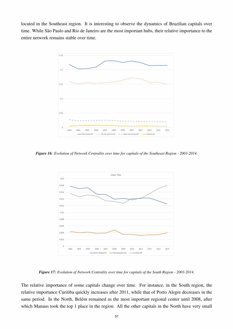
located in the Southeast region. It is interesting to observe the dynamics of Brazilian capitals overtime. While Sao Paulo and Rio de Janeiro are the most important hubs, their relative importance to theentire network remains stable over time.
0
0.05
0.1
0.15
0.2
0.25
2003 2004 2005 2006 2007 2008 2009 2010 2011 2012 2013 2014
São Paulo DC Rio de Janeiro DC Belo Horizonte DC Vitória DC
Figure 16: Evolution of Network Centrality over time for capitals of the Southeast Region - 2003-2014.
0
0.002
0.004
0.006
0.008
0.01
0.012
0.014
0.016
0.018
0.02
2003 2004 2005 2006 2007 2008 2009 2010 2011 2012 2013 2014
Chart Title
Porto Alegre DC Florianópolis DC Curitiba DC
Figure 17: Evolution of Network Centrality over time for capitals of the South Region - 2003-2014.
The relative importance of some capitals change over time. For instance, in the South region, therelative importance Curitiba quickly increases after 2011, while that of Porto Alegre decreases in thesame period. In the North, Belem remained as the most important regional center until 2008, afterwhich Manaus took the top 1 place in the region. All the other capitals in the North have very small
57
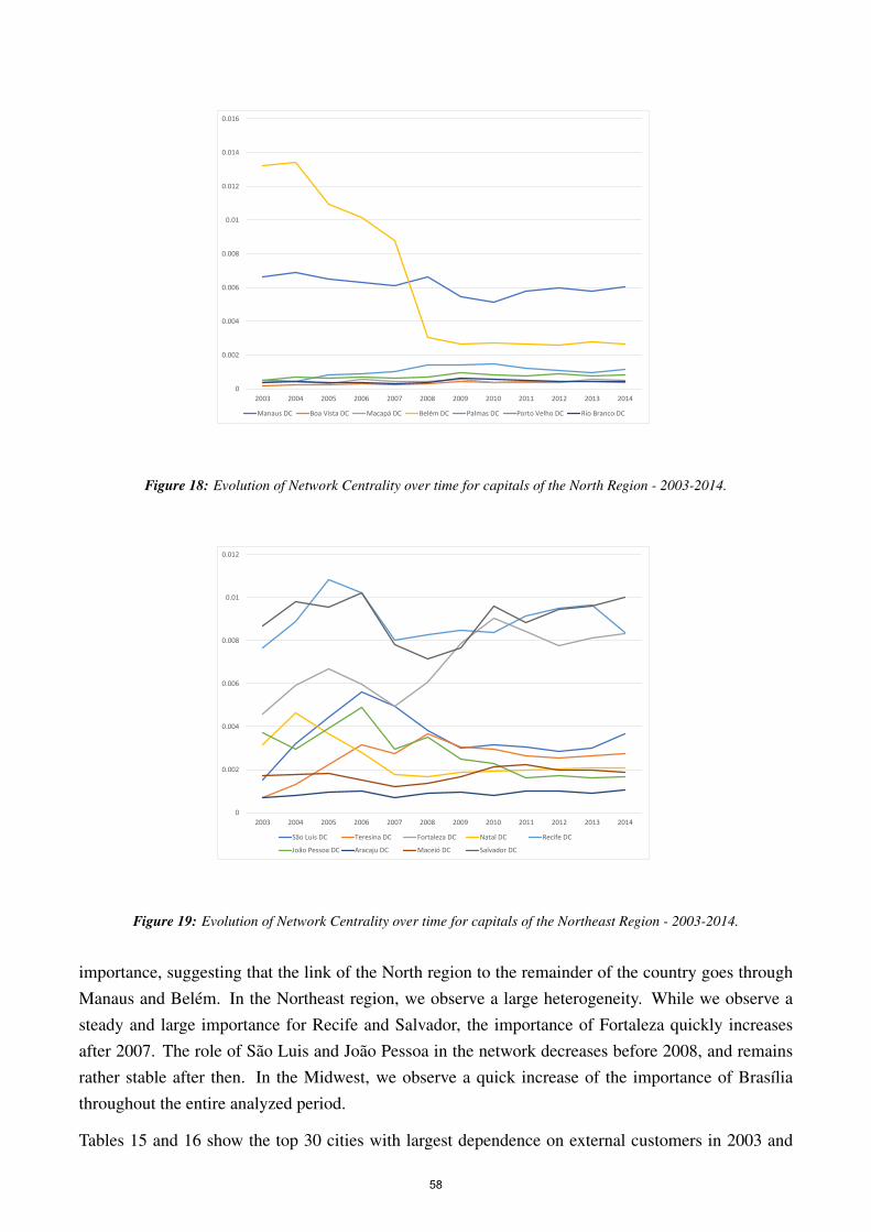
0
0.002
0.004
0.006
0.008
0.01
0.012
0.014
0.016
2003 2004 2005 2006 2007 2008 2009 2010 2011 2012 2013 2014
Manaus DC Boa Vista DC Macapá DC Belém DC Palmas DC Porto Velho DC Rio Branco DC
Figure 18: Evolution of Network Centrality over time for capitals of the North Region - 2003-2014.
0
0.002
0.004
0.006
0.008
0.01
0.012
2003 2004 2005 2006 2007 2008 2009 2010 2011 2012 2013 2014
São Luís DC Teresina DC Fortaleza DC Natal DC Recife DC
João Pessoa DC Aracaju DC Maceió DC Salvador DC
Figure 19: Evolution of Network Centrality over time for capitals of the Northeast Region - 2003-2014.
importance, suggesting that the link of the North region to the remainder of the country goes throughManaus and Belem. In the Northeast region, we observe a large heterogeneity. While we observe asteady and large importance for Recife and Salvador, the importance of Fortaleza quickly increasesafter 2007. The role of Sao Luis and Joao Pessoa in the network decreases before 2008, and remainsrather stable after then. In the Midwest, we observe a quick increase of the importance of Brasıliathroughout the entire analyzed period.
Tables 15 and 16 show the top 30 cities with largest dependence on external customers in 2003 and
58
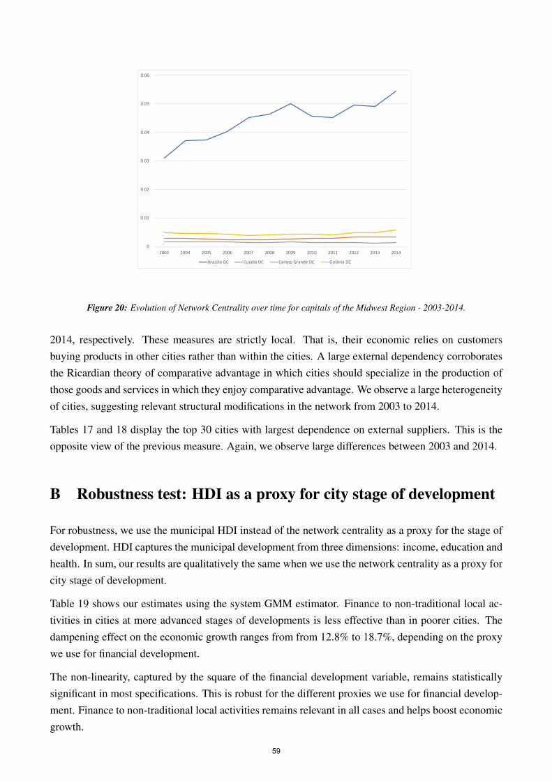
0
0.01
0.02
0.03
0.04
0.05
0.06
2003 2004 2005 2006 2007 2008 2009 2010 2011 2012 2013 2014
Brasília DC Cuiabá DC Campo Grande DC Goiânia DC
Figure 20: Evolution of Network Centrality over time for capitals of the Midwest Region - 2003-2014.
2014, respectively. These measures are strictly local. That is, their economic relies on customersbuying products in other cities rather than within the cities. A large external dependency corroboratesthe Ricardian theory of comparative advantage in which cities should specialize in the production ofthose goods and services in which they enjoy comparative advantage. We observe a large heterogeneityof cities, suggesting relevant structural modifications in the network from 2003 to 2014.
Tables 17 and 18 display the top 30 cities with largest dependence on external suppliers. This is theopposite view of the previous measure. Again, we observe large differences between 2003 and 2014.
B Robustness test: HDI as a proxy for city stage of development
For robustness, we use the municipal HDI instead of the network centrality as a proxy for the stage ofdevelopment. HDI captures the municipal development from three dimensions: income, education andhealth. In sum, our results are qualitatively the same when we use the network centrality as a proxy forcity stage of development.
Table 19 shows our estimates using the system GMM estimator. Finance to non-traditional local ac-tivities in cities at more advanced stages of developments is less effective than in poorer cities. Thedampening effect on the economic growth ranges from from 12.8% to 18.7%, depending on the proxywe use for financial development.
The non-linearity, captured by the square of the financial development variable, remains statisticallysignificant in most specifications. This is robust for the different proxies we use for financial develop-ment. Finance to non-traditional local activities remains relevant in all cases and helps boost economicgrowth.
59

Table 15: This Table presents the Ranking of 30 Municipalities with the largest Dependence on External Customers for theyear 2003.
Ranking DOEC Municipality State Region1 0.795370826 Brasılia Distrito Federal Midwest2 0.416008792 Sao Paulo Sao Paulo Southeast3 0.83235105 Barueri Sao Paulo Southeast4 0.586766546 Rio de Janeiro Rio de Janeiro Southeast5 0.631166157 Belo Horizonte Minas Gerais Southeast6 0.531294203 Curitiba Parana South7 0.468052589 Porto Alegre Rio Grande do Sul South8 0.759992403 Recife Pernambuco Northeast9 0.305556972 Belem Para North10 0.63239366 Salvador Bahia Northeast11 0.454881681 Fortaleza Ceara Northeast12 0.465568416 Goiania Goias Midwest13 0.511900065 Joao Pessoa Paraıba Northeast14 0.718979751 Campinas Sao Paulo Southeast15 0.814474683 Sao Jose do Rio Preto Sao Paulo Southeast16 0.921534455 Guarulhos Sao Paulo Southeast17 0.861665804 Sao Bernardo do Campo Sao Paulo Southeast18 0.838778323 Vitoria Espırito Santo Southeast19 0.772825347 Manaus Amazonas North20 0.714110626 Uberlandia Minas Gerais Southeast21 0.89849591 Contagem Minas Gerais Southeast22 0.86174688 Osasco Sao Paulo Southeast23 0.87719539 Sao Caetano do Sul Sao Paulo Southeast24 0.708113867 Cuiaba Mato Grosso Midwest25 0.636841338 Caxias do Sul Rio Grande do Sul South26 0.806064454 Ribeirao Preto Sao Paulo Southeast27 0.903613025 Londrina Parana South28 0.954008776 Santana de Parnaıba Sao Paulo Southeast29 0.698280039 Florianopolis Santa Catarina South30 0.492868244 Maceio Alagoas Northeast
60

Table 16: This Table presents the Ranking of 30 Municipalities with the largest Dependence on External Customers for theyear 2014.
Ranking DOEC Municipality State Region1 1 Cachoeira Grande Maranhao Northeast2 1 Sao Goncalo do Gurgueia Piauı Northeast3 1 Jardim de Angicos Rio Grande do Norte Northeast4 1 Vila Flor Rio Grande do Norte Northeast5 1 Curral Velho Paraıba Northeast6 1 Sao Jose de Princesa Paraıba Northeast7 1 Serra Redonda Paraıba Northeast8 0.997122506 Tupirama Tocantins North9 0.996206118 Serra do Navio Amapa North10 0.995532866 Pau D’Arco do Piauı Piauı Northeast11 0.993259048 Peixe Tocantins North12 0.992789406 Parari Paraıba Northeast13 0.990008895 Piau Minas Gerais Southeast14 0.986523308 Passagem Franca do Piauı Piauı Northeast15 0.98649516 Sao Miguel das Matas Bahia Northeast16 0.98395192 Pedro Laurentino Piauı Northeast17 0.983502794 Treviso Santa Catarina South18 0.981818252 Rafard Sao Paulo Southeast19 0.980891621 Agua Nova Rio Grande do Norte Northeast20 0.980171197 Salmourao Sao Paulo Southeast21 0.97966321 Salgado de Sao Felix Paraıba Northeast22 0.976501142 Major Gercino Santa Catarina South23 0.976064598 Quata Sao Paulo Southeast24 0.975074776 Vicosa Rio Grande do Norte Northeast25 0.974293568 Mutuıpe Bahia Northeast26 0.97410688 Jenipapo de Minas Minas Gerais Southeast27 0.972538086 Sao Francisco do Para Para North28 0.971517816 Bom Jardim da Serra Santa Catarina South29 0.971370019 Sao Miguel da Baixa Grande Piauı Northeast30 0.971009887 Areia de Baraunas Paraıba Northeast
61
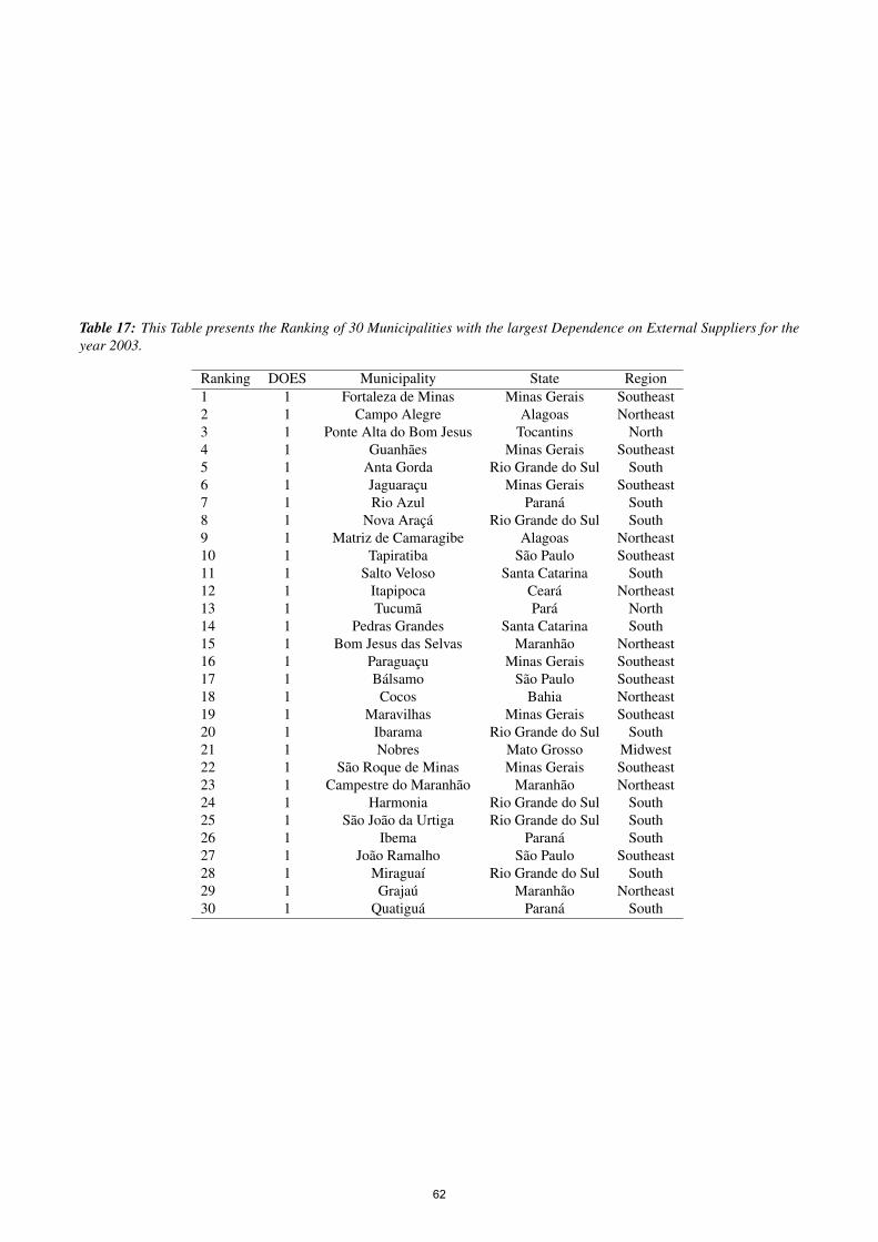
Table 17: This Table presents the Ranking of 30 Municipalities with the largest Dependence on External Suppliers for theyear 2003.
Ranking DOES Municipality State Region1 1 Fortaleza de Minas Minas Gerais Southeast2 1 Campo Alegre Alagoas Northeast3 1 Ponte Alta do Bom Jesus Tocantins North4 1 Guanhaes Minas Gerais Southeast5 1 Anta Gorda Rio Grande do Sul South6 1 Jaguaracu Minas Gerais Southeast7 1 Rio Azul Parana South8 1 Nova Araca Rio Grande do Sul South9 1 Matriz de Camaragibe Alagoas Northeast10 1 Tapiratiba Sao Paulo Southeast11 1 Salto Veloso Santa Catarina South12 1 Itapipoca Ceara Northeast13 1 Tucuma Para North14 1 Pedras Grandes Santa Catarina South15 1 Bom Jesus das Selvas Maranhao Northeast16 1 Paraguacu Minas Gerais Southeast17 1 Balsamo Sao Paulo Southeast18 1 Cocos Bahia Northeast19 1 Maravilhas Minas Gerais Southeast20 1 Ibarama Rio Grande do Sul South21 1 Nobres Mato Grosso Midwest22 1 Sao Roque de Minas Minas Gerais Southeast23 1 Campestre do Maranhao Maranhao Northeast24 1 Harmonia Rio Grande do Sul South25 1 Sao Joao da Urtiga Rio Grande do Sul South26 1 Ibema Parana South27 1 Joao Ramalho Sao Paulo Southeast28 1 Miraguaı Rio Grande do Sul South29 1 Grajau Maranhao Northeast30 1 Quatigua Parana South
62
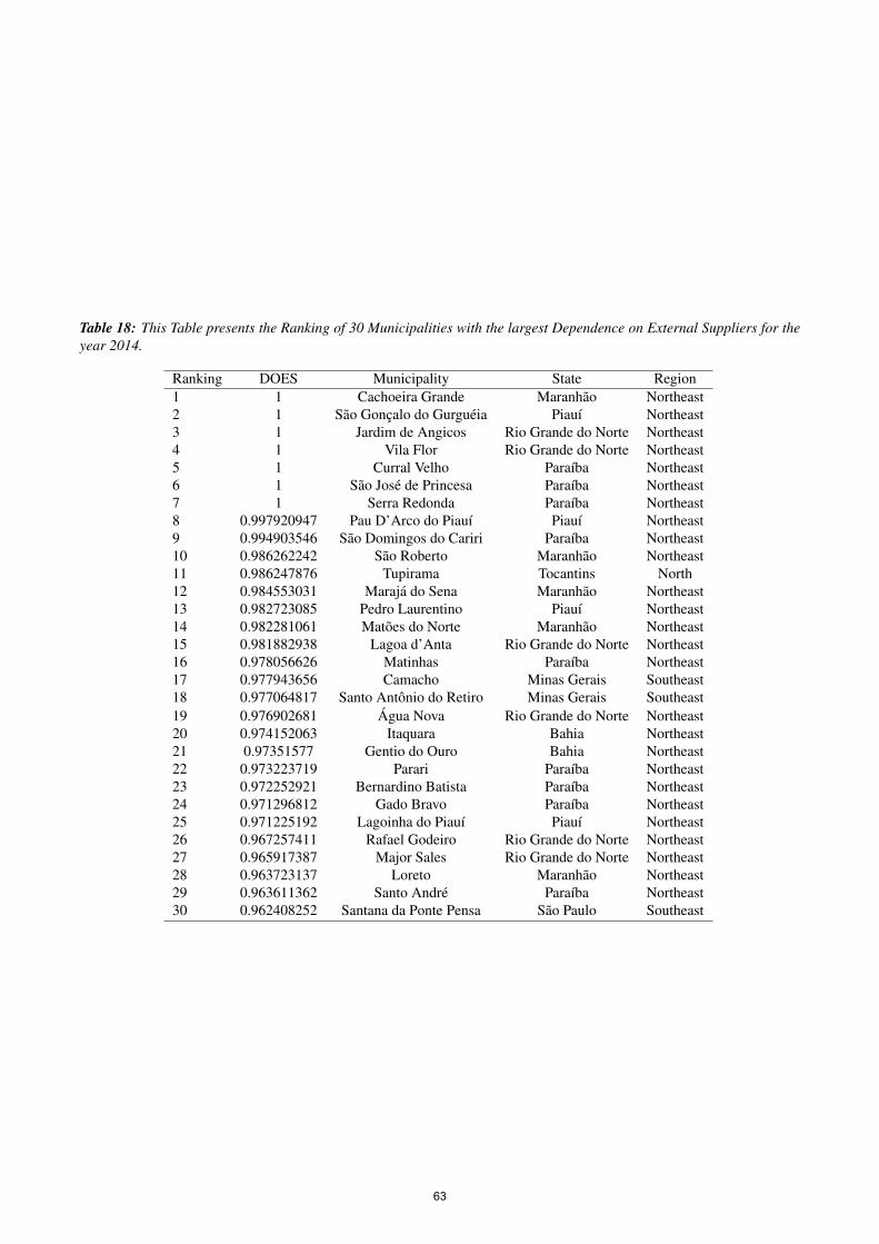
Table 18: This Table presents the Ranking of 30 Municipalities with the largest Dependence on External Suppliers for theyear 2014.
Ranking DOES Municipality State Region1 1 Cachoeira Grande Maranhao Northeast2 1 Sao Goncalo do Gurgueia Piauı Northeast3 1 Jardim de Angicos Rio Grande do Norte Northeast4 1 Vila Flor Rio Grande do Norte Northeast5 1 Curral Velho Paraıba Northeast6 1 Sao Jose de Princesa Paraıba Northeast7 1 Serra Redonda Paraıba Northeast8 0.997920947 Pau D’Arco do Piauı Piauı Northeast9 0.994903546 Sao Domingos do Cariri Paraıba Northeast10 0.986262242 Sao Roberto Maranhao Northeast11 0.986247876 Tupirama Tocantins North12 0.984553031 Maraja do Sena Maranhao Northeast13 0.982723085 Pedro Laurentino Piauı Northeast14 0.982281061 Matoes do Norte Maranhao Northeast15 0.981882938 Lagoa d’Anta Rio Grande do Norte Northeast16 0.978056626 Matinhas Paraıba Northeast17 0.977943656 Camacho Minas Gerais Southeast18 0.977064817 Santo Antonio do Retiro Minas Gerais Southeast19 0.976902681 Agua Nova Rio Grande do Norte Northeast20 0.974152063 Itaquara Bahia Northeast21 0.97351577 Gentio do Ouro Bahia Northeast22 0.973223719 Parari Paraıba Northeast23 0.972252921 Bernardino Batista Paraıba Northeast24 0.971296812 Gado Bravo Paraıba Northeast25 0.971225192 Lagoinha do Piauı Piauı Northeast26 0.967257411 Rafael Godeiro Rio Grande do Norte Northeast27 0.965917387 Major Sales Rio Grande do Norte Northeast28 0.963723137 Loreto Maranhao Northeast29 0.963611362 Santo Andre Paraıba Northeast30 0.962408252 Santana da Ponte Pensa Sao Paulo Southeast
63
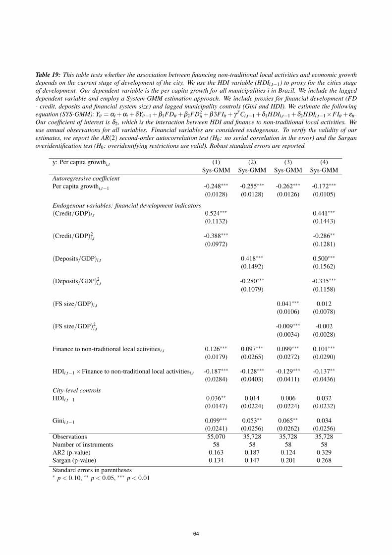
Table 19: This table tests whether the association between financing non-traditional local activities and economic growthdepends on the current stage of development of the city. We use the HDI variable (HDIi,t−1) to proxy for the cities stageof development. Our dependent variable is the per capita growth for all municipalities i in Brazil. We include the laggeddependent variable and employ a System-GMM estimation approach. We include proxies for financial development (FD- credit, deposits and financial system size) and lagged municipality controls (Gini and HDI). We estimate the followingequation (SYS-GMM): Yit = αi+αt +δYit−1+β1FDit +β2FD2
it +β3FIit +γTCi,t−1+δ1HDIi,t−1+δ2HDIi,t−1×FIit +εit .Our coefficient of interest is δ2, which is the interaction between HDI and finance to non-traditional local activities. Weuse annual observations for all variables. Financial variables are considered endogenous. To verify the validity of ourestimates, we report the AR(2) second-order autocorrelation test (H0: no serial correlation in the error) and the Sarganoveridentification test (H0: overidentifying restrictions are valid). Robust standard errors are reported.
y: Per capita growthi,t (1) (2) (3) (4)Sys-GMM Sys-GMM Sys-GMM Sys-GMM
Autoregressive coefficientPer capita growthi,t−1 -0.248∗∗∗ -0.255∗∗∗ -0.262∗∗∗ -0.172∗∗∗
(0.0128) (0.0128) (0.0126) (0.0105)
Endogenous variables: financial development indicators(Credit/GDP)i,t 0.524∗∗∗ 0.441∗∗∗
(0.1132) (0.1443)
(Credit/GDP)2i,t -0.388∗∗∗ -0.286∗∗
(0.0972) (0.1281)
(Deposits/GDP)i,t 0.418∗∗∗ 0.500∗∗∗
(0.1492) (0.1562)
(Deposits/GDP)2i,t -0.280∗∗∗ -0.335∗∗∗
(0.1079) (0.1158)
(FS size/GDP)i,t 0.041∗∗∗ 0.012(0.0106) (0.0078)
(FS size/GDP)2i,t -0.009∗∗∗ -0.002
(0.0034) (0.0028)
Finance to non-traditional local activitiesi,t 0.126∗∗∗ 0.097∗∗∗ 0.099∗∗∗ 0.101∗∗∗
(0.0179) (0.0265) (0.0272) (0.0290)
HDIi,t−1×Finance to non-traditional local activitiesi,t -0.187∗∗∗ -0.128∗∗∗ -0.129∗∗∗ -0.137∗∗
(0.0284) (0.0403) (0.0411) (0.0436)
City-level controlsHDIi,t−1 0.036∗∗ 0.014 0.006 0.032
(0.0147) (0.0224) (0.0224) (0.0232)
Ginii,t−1 0.099∗∗∗ 0.053∗∗ 0.065∗∗ 0.034(0.0241) (0.0256) (0.0262) (0.0256)
Observations 55,070 35,728 35,728 35,728Number of instruments 58 58 58 58AR2 (p-value) 0.163 0.187 0.124 0.329Sargan (p-value) 0.134 0.147 0.201 0.268Standard errors in parentheses∗ p < 0.10, ∗∗ p < 0.05, ∗∗∗ p < 0.01
64