Embed Size (px)
Citation preview

Third-order Smoothness Helps: Even Faster Stochastic
Optimization Algorithms for Finding Local Minima
Yaodong Yu∗‡ and Pan Xu†‡ and Quanquan Gu§
Abstract
We propose stochastic optimization algorithms that can find local minima faster than existing
algorithms for nonconvex optimization problems, by exploiting the third-order smoothness to
escape non-degenerate saddle points more efficiently. More specifically, the proposed algorithm
only needs O(ε−10/3) stochastic gradient evaluations to converge to an approximate local minimum
x, which satisfies ‖∇f(x)‖2 ≤ ε and λmin(∇2f(x)) ≥ −√ε in the general stochastic optimization
setting, where O(·) hides logarithm polynomial terms and constants. This improves upon the
O(ε−7/2) gradient complexity achieved by the state-of-the-art stochastic local minima finding
algorithms by a factor of O(ε−1/6). For nonconvex finite-sum optimization, our algorithm also
outperforms the best known algorithms in a certain regime.
1 Introduction
We study the following problem of unconstrained stochastic optimization
minx∈Rd
f(x) = Eξ∼D[F (x; ξ)], (1.1)
where F (x; ξ) : Rd → R is a stochastic function and ξ is a random variable sampled from a fixed
distribution D. In particular, we are interested in nonconvex optimization where the expected
function f(x) is nonconvex. Note that (1.1) also covers the finite sum optimization problem, where
f(x) = 1/n∑n
i=1 fi(x), which can be seen as a special case of stochastic optimization when the
random variable ξ follows a uniform distribution over {1, . . . , n}. This kind of nonconvex optimization
is ubiquitous in machine learning, especially deep learning (LeCun et al., 2015). Finding a global
minimum of nonconvex problem (1.1) is generally NP hard (Hillar and Lim, 2013). Nevertheless,
for many nonconvex optimization in machine learning, a local minimum is adequate and can be as
good as a global minimum in terms of generalization performance, especially in many deep learning
problems (Choromanska et al., 2015; Dauphin et al., 2014).
∗Department of Computer Science, University of Virginia, Charlottesville, VA 22904, USA; e-
mail:[email protected]†Department of Computer Science, University of Virginia, Charlottesville, VA 22904, USA; e-mail:
[email protected]‡Equal Contribution§Department of Computer Science, University of Virginia, Charlottesville, VA 22904, USA; e-mail:
1
arX
iv:1
712.
0658
5v1
[m
ath.
OC
] 1
8 D
ec 2
017

In this paper, we aim to design efficient stochastic optimization algorithms that can find an
approximate local minimum of (1.1), i.e., an (ε, εH)-second-order stationary point defined as follows
‖∇f(x)‖2 ≤ ε, and λmin
(∇2f(x)
)≥ −εH , (1.2)
where ε, εH ∈ (0, 1). Notably, when εH =√L2ε for Hessian Lipschitz f(·) with parameter L2,
(1.2) is equivalent to the definition of ε-second-order stationary point (Nesterov and Polyak, 2006).
Algorithms based on cubic regularized Newton’s method (Nesterov and Polyak, 2006) and its variants
(Agarwal et al., 2016; Carmon and Duchi, 2016; Curtis et al., 2017; Kohler and Lucchi, 2017; Xu
et al., 2017; Tripuraneni et al., 2017) have been proposed to find the approximate local minimum.
However, all of them need to solve the cubic problems exactly (Nesterov and Polyak, 2006) or
approximately (Agarwal et al., 2016; Carmon and Duchi, 2016) in each iteration, which poses a
rather heavy computational overhead. Another line of research employs the negative curvature
direction to find the local minimum by combining accelerated gradient descent and negative curvature
descent (Carmon et al., 2016; Allen-Zhu, 2017), which becomes impractical in large scale and high
dimensional machine learning problems due to the frequent computation of negative curvature in
each iteration.
To alleviate the computational burden of local minimum finding algorithms, there has emerged
a fresh line of research (Xu and Yang, 2017; Allen-Zhu and Li, 2017b; Jin et al., 2017b; Yu et al.,
2017) that tries to achieve the iteration complexity as the state-of-the-art second-order methods,
while only utilizing first-order oracles. The key observation is that first-order methods with noise
injection (Ge et al., 2015; Jin et al., 2017a) are essentially an equivalent way to extract the negative
curvature direction at saddle points (Xu and Yang, 2017; Allen-Zhu and Li, 2017b). With first-
order information and the state-of-the-art Stochastically Controlled Stochastic Gradient (SCSG)
method (Lei et al., 2017), the aforementioned methods (Xu and Yang, 2017; Allen-Zhu and Li, 2017b)
converge to an (ε,√ε)-second-order stationary point (an approximate local minimum) within O(ε−7/2)
stochastic gradient evaluations, where O(·) hides logarithm polynomial factors and constants. In
this work, motivated by Carmon et al. (2017) which employed the third-order smoothness of f(·) in
deterministic nonconvex optimization and proposed an algorithm that converges to a first-order
stationary point with O(ε−5/3) full gradient evaluations, we explore the benefits of third-order
smoothness in finding an approximate local minimum in the stochastic nonconvex optimization
setting. In particular, we propose a stochastic optimization algorithm that only utilizes first-order
oracles and finds the (ε, εH)-second-order stationary point within O(ε−10/3) stochastic gradient
evaluations. Note that our gradient complexity matches that of the state-of-the-art stochastic
optimization algorithm SCSG (Lei et al., 2017) for finding first-order stationary points. At the
core of our algorithm is an exploitation of the third-order smoothness of the objective function f(·)which enables us to choose a larger step size in the negative curvature descent stage, and therefore
leads to a faster convergence rate. The main contributions of our work are summarized as follows
• We show that third-order smoothness of nonconvex function can lead to a faster escape
from saddle points in the stochastic optimization. We characterize, for the first time, the
improvement brought by third-order smoothness in finding the negative curvature direction.
• We propose efficient stochastic algorithms for both finite-sum and general stochastic objective
functions and prove faster convergence rates for finding local minima. More specifically, for
2

finite-sum setting, the proposed algorithm converges to an (ε, εH)-second-order stationary
point within O(n2/3ε−2 + nε−2H + n3/4ε−5/2H ) stochastic gradient evaluations, and for general
stochastic optimization setting, our algorithm converges to an approximate local minimum
with only O(ε−10/3) stochastic gradient evaluations.
• In each outer iteration, our proposed algorithms only need to call either one negative curvature
descent step, or an epoch of SCSG. Compared with existing algorithms which need to execute
at least one of these two procedures or even both in each outer iteration, our algorithms save
a lot of gradient and negative curvature computations.
The remainder of this paper is organized as follows: We review the related work in Section 2, and
present some preliminary definitions in Section 3. In Section 4, we elaborate the motivation of using
third-order smoothness and present faster negative curvature descent algorithms in finite-sum and
stochastic settings. In Section 5, we present local minima finding algorithms and the corresponding
theoretical analyses for both finite-sum and general stochastic nonconvex optimization problems.
Finally, we conclude our paper in Section 6.
Notation We use A = [Aij ] ∈ Rd×d to denote a matrix and x = (x1, ..., xd)> ∈ Rd to denote a
vector. Let ‖x‖q = (∑d
i=1 |xi|q)1/q be `q vector norm for 0 < q < +∞. We use ‖A‖2 and ‖A‖Fto denote the spectral and Frobenius norm of A. For a three-way tensor T ∈ Rd×d×d and vector
x ∈ Rd, we denote the inner product as 〈T ,x⊗3〉. For a symmetric matrix A, let λmax(A) and
λmin(A) be the maximum, minimum eigenvalues of matrix A. We use A � 0 to denote A is positive
semidefinite. For any two sequences {an} and {bn}, if an ≤ C bn for some 0 < C < +∞ independent
of n, we write an = O(bn). The notation O(·) hides logarithmic factors. For sequences fn, gn, if fnis less than (larger than) gn up to a constant, then we write fn . gn (fn & gn).
2 Related Work
In this section, we discuss related work for finding approximate second-order stationary points in
nonconvex optimization. Roughly speaking, existing literature can be divided into the following
three categories.
Hessian-based: The pioneer work of Nesterov and Polyak (2006) proposed the cubic regularized
Newton’s method to find an (ε, εH)-second-order stationary point in O(
max{ε−3/2, ε−3H })
iterations.
Curtis et al. (2017) showed that the trust-region Newton method can achieve the same iteration
complexity as the cubic regularization method. Recently, Kohler and Lucchi (2017); Xu et al. (2017)
showed that by using subsampled Hessian matrix instead of the entire Hessian matrix in cubic
regularization method and trust-region method, the iteration complexity can still match the original
exact methods under certain conditions. However, these methods need to compute the Hessian
matrix and solve a very expensive subproblem either exactly or approximately in each iteration,
which can be computationally intractable for high-dimensional problems.
Hessian-vector product-based: Through different approaches, Carmon et al. (2016) and Agarwal
et al. (2016) independently proposed algorithms that are able to find (ε,√ε)-second-order stationary
points with O(ε−7/4) full gradient and Hessian-vector product evaluations. By making an additional
assumption of the third-order smoothness on the objective function and combining the negative
curvature descent with the “convex until proven guilty” algorithm, Carmon et al. (2017) proposed
3

an algorithm that is able to find an (ε,√ε)-second-order stationary point with O(ε−5/3) full gradient
and Hessian-vector product evaluations.1 Agarwal et al. (2016) also considered the finite-sum
nonconvex optimization and proposed algorithm which is able to find approximate local minima
within O(nε−3/2 + n3/4ε−7/2) stochastic gradient and stochastic Hessian-vector product evaluations.
For nonconvex finite-sum problems, Reddi et al. (2017) proposed an algorithm, which is a combination
of first-order and second-order methods to find approximate (ε, εH)-second-order stationary points,
and requires O(n2/3ε−2+nε−3H +n3/4ε
−7/2H
)stochastic gradient and stochastic Hessian-vector product
evaluations. In the general stochastic optimization setting, Allen-Zhu (2017) proposed an algorithm
named Natasha2, which is based on variance reduction and negative curvature descent, and is
able to find (ε,√ε)-second-order stationary points with at most O(ε−7/2) stochastic gradient and
stochastic Hessian-vector product evaluations. Tripuraneni et al. (2017) proposed a stochastic
cubic regularization algorithm to find (ε,√ε)-second-order stationary points and achieved the same
runtime complexity as Allen-Zhu (2017).
Gradient-based: For general nonconvex problems, Levy (2016); Jin et al. (2017a,b) showed that
it is possible to escape from saddle points and find local minima by using gradient evaluations plus
random perturbation. The best-known runtime complexity of these methods is O(ε−7/4
)when
setting εH =√ε, which is proposed in Jin et al. (2017b). In the nonconvex finite-sum setting,
Allen-Zhu and Li (2017b) proposed a first-order negative curvature finding method called Neon2
and applied it to the nonconvex stochastic variance reduced gradient (SVRG) method (Reddi
et al., 2016; Allen-Zhu and Hazan, 2016; Lei et al., 2017), which gives rise to an algorithm to find
(ε, εH)-second-order stationary points with O(n2/3ε−2 +nε−3H +n3/4ε
−7/2H +n5/12ε−2ε−1/2H
)stochastic
gradient evaluations. For nonconvex stochastic optimization problems, a variant of stochastic
gradient descent (SGD) in Ge et al. (2015) is proved to find the (ε,√ε)-second-order stationary
point with O(ε−4poly(d)) stochastic gradient evaluations. Recently, Xu and Yang (2017); Allen-
Zhu and Li (2017b) turned the stochastically controlled stochastic gradient (SCSG) method (Lei
et al., 2017) into approximate local minima finding algorithms, which involves stochastic gradient
computation. The runtime complexity of these algorithms is O(ε−10/3 + ε−2ε−3H ). Very recently,
in order to further save gradient and negative curvature computations, Yu et al. (2017) proposed
a family of new algorithms called GOSE, which can find (ε, εH)-second-order stationary points
with O(ε−7/4 +
(ε−1/4 + ε
−1/2H
)min
{ε−3H , Nε
})gradient evaluations in the deterministic setting,
O(n2/3ε−2 +
(n+n3/4ε
−1/2H
)min
{ε−3H , Nε
})stochastic gradient evaluations in the finite-sum setting,
and O(ε−10/3 + ε−2ε−3H +
(ε−2 + ε−2H
)min
{ε−3H , Nε
})stochastic gradient evaluations in the general
stochastic setting, where Nε is the number of saddle points encountered by the algorithms until they
find an approximate local minimum. Provided that Nε is smaller than ε−3H , the runtime complexity
is better than the state-of-the-art (Allen-Zhu and Li, 2017b; Jin et al., 2017b). However, none of
the above gradient-based algorithms explore the third-order smoothness of the nonconvex objective
function.
1As shown in Carmon et al. (2017), the second-order accuracy parameter εH can be set as ε2/3 and the total
runtime complexity remains the same, i.e., O(ε−5/3).
4

3 Preliminaries
In this section, we present some definitions which will be used in our algorithm design and later
theoretical analysis.
Definition 3.1 (Smoothness). A differentiable function f(·) is L1-smooth, if for any x, y ∈ Rd:
‖∇f(x)−∇f(y)‖2 ≤ L1‖x− y‖2.
Definition 3.2 (Hessian Lipschitz). A twice-differentiable function f(·) is L2-Hessian Lipschitz, if
for any x, y ∈ Rd:‖∇2f(x)−∇2f(y)‖2 ≤ L2‖x− y‖2.
Note that the Hessian-Lipschitz is also referred to as second-order smoothness. The above two
smoothness conditions are widely used in nonconvex optimization problems (Nesterov and Polyak,
2006). In this paper, we will explore the third-order derivative Lipschitz condition. Here we use
a three-way tensor ∇3f(x) ∈ Rd×d×d to denote the third-order derivative of a function, which is
formally defined below.
Definition 3.3 (Third-order Derivative). The third-order derivative of function f(·): Rd → R is a
three-way tensor ∇3f(x) ∈ Rd×d×d which is defined as
[∇3f(x)]ijk =∂
∂xi∂xj∂xkf(x) for i, j, k = 1, . . . , d and x ∈ Rd.
Next we introduce the third-order smooth condition of function f(·), which implies that the
third-order derivative will not change rapidly.
Definition 3.4 (Third-order derivative Lipschitz). A thrice-differentiable function f(·) has L3-
Lipschitz third-order derivative, if for any x, y ∈ Rd:
‖∇3f(x)−∇3f(y)‖F ≤ L3‖x− y‖2.
The above definition has been introduced in Anandkumar and Ge (2016), and the third-order
derivative Lipschitz is also referred to as third-order smoothness in Carmon et al. (2017). One can
also use another equivalent notion of third-order derivative Lipschitz condition used in Carmon et al.
(2017). Note that the third-order Lipschitz condition is critical in our algorithms and theoretical
analysis in later sections. In the sequel, we will use third-order derivative Lipschitz and third-order
smoothness interchangeably.
Definition 3.5 (Optimal Gap). For a function f(·), we define ∆f as
f(x0)− infx∈Rd
f(x) ≤ ∆f ,
and without loss of generality, we throughout assume ∆f < +∞.
Definition 3.6 (Geometric Distribution). For a random integer X, define X has a geometric
distribution with parameter p, denoted as Geom(p), if it satisfies that
P(X = k) = pk(1− p), ∀k = 0, 1, . . . .
5

Definition 3.7 (Sub-Gaussian Stochastic Gradient). For any x ∈ Rd and random variable ξ ∈ D,
the stochastic gradient ∇F (x; ξ) is sub-Gaussian with parameter σ if it satisfies
E[
exp
(‖∇F (x; ξ)−∇f(x)‖22σ2
)]≤ exp(1).
In addition, we introduce Tg to denote the time complexity of stochastic gradient evaluation,
and Th to denote the time complexity of stochastic Hessian-vector product evaluation.
4 Exploiting Third-order Smoothness
In this section we will show how to exploit the third-order smoothness of the objective function to
make better use of the negative curvature direction for escaping saddle points. To begin with, we
will first explain why third-order smoothness helps in general nonconvex optimization problems.
Then we present two algorithms which are able to utilize the third-order smoothness to take a larger
step size in the finite-sum setting and the stochastic setting.
In order to find local minima in nonconvex problems, different kinds of approaches have been
explored to escape from saddle points. One of these approaches is to use negative curvature direction
(More and Sorensen, 1979) to escape from saddle points, which has been explored in many previous
studies (Carmon et al., 2016; Allen-Zhu, 2017). According to some recent work (Xu and Yang,
2017; Allen-Zhu and Li, 2017b), it is possible to extract the negative curvature direction by only
using (stochastic) gradient evaluations, which makes the negative curvature descent approach more
appealing.
We first consider a simple case to illustrate how to utilize the third-order smoothness when
taking a negative curvature descent step. For nonconvex optimization problems, an ε-first-order
stationary point x can be found by using first-order methods, such as gradient descent. Suppose an
ε-first-order stationary point x is not an (ε, εH)-first-order stationary point, which means that there
exists a unit vector v such that
v>∇2f(x) v ≤ −εH2.
Following the previous work (Carmon et al., 2016; Xu and Yang, 2017; Allen-Zhu and Li, 2017b; Yu
et al., 2017), one can take a negative curvature descent step along v to escape from the saddle point
x , i.e.,
y = argminy∈{u,w}
f(y), where u = x− α v, w = x + α v and α = O
(εHL2
). (4.1)
Suppose the function f(·) is L1-smooth and L2-Hessian Lipschitz, then the negative curvature
descent step (4.1) is guaranteed to make the function value decrease,
f(y)− f(x) = −O(ε3HL22
). (4.2)
Inspired by the previous work (Carmon et al., 2017), incorporating with an additional assumption
that the objective function has L3-Lipschitz third-order derivatives (third-order smoothness) can
help achieve better convergence rate for nonconvex problems. More specifically, we can adjust the
6

update as follows,
y = argminy∈{u,w}
f(y), where u = x− η v, w = x + η v and η = O
(√εHL3
). (4.3)
Note that the adjusted step size η can be much larger than the step size α in (4.1). Moreover, the
adjusted negative curvature descent step (4.3) is guaranteed to decrease the function value by a
larger decrement, i.e.,
f(y)− f(x) = −O(ε2HL3
). (4.4)
Compared with (4.2), the decrement in (4.4) can be substantially larger. In other words, if we make
the additional assumption of the third-order smoothness, the negative curvature descent with larger
step size will make more progress toward decreasing the function value.
In the following, we will exploit the benefits of third-order smoothness in escaping from saddle
points for stochastic nonconvex optimization.
4.1 Special Stochastic Optimization with Finite-Sum Structures
We first consider the following finite-sum problem, which is a special case of (1.1).
minx∈Rd
f(x) =1
n
n∑
i=1
fi(x), (4.5)
where fi(·) is possibly nonconvex. Algorithms in this setting have access to the information of
each individual function fi(·) and the entire function f(·). For the finite-sum structure, variance
reduction-based methods (Reddi et al., 2016; Allen-Zhu and Hazan, 2016; Garber et al., 2016) can
be applied to improve the gradient complexity of different nonconvex optimization algorithms.
We first present two different approaches to find the negative curvature direction in the finite-sum
setting. The approximate leading eigenvector computation methods (Kuczynski and Wozniakowski,
1992; Garber et al., 2016) can be used to estimate the negative curvature direction, which are
denoted by FastPCA methods in the sequel. To find the negative curvature direction of function
f(·) at point x, we can estimate the eigenvector with the smallest eigenvalue of a Hessian matrix
H = ∇2f(x). Since the function f(·) is L1-smooth, one can instead estimate the eigenvector with
the largest eigenvalue of the shifted matrix M = L1 · I−H. Therefore, we can apply FastPCA for
finite-sum problems to find the such eigenvector of the matrix M, and we describe its result in the
following lemma.
Lemma 4.1. (Garber et al., 2016) Let f(x) = 1/n∑n
i=1 fi(x) where each component function fi(x)
is twice-differentiable and L1-smooth. For any given point x ∈ Rd, if λmin(∇2f(x)) ≤ −εH , then
with probability at least 1− δ, Shifted-and-Inverted power method returns a unit vector v satisfying
v>∇2f(x) v < −εH2,
with O((n+ n3/4
√L1/εH) log3(d) log(1/δ)
)stochastic Hessian-vector product evaluations.
7

Different from FastPCA-type methods, there is another type of approaches to compute the
negative curvature direction without using the Hessian-vector product evaluation. In detail, Xu and
Yang (2017); Allen-Zhu and Li (2017b) proposed algorithms that are able to extract the negative
curvature direction based on random perturbation and (stochastic) gradient evaluation, and we
denote these methods by Neon2 in the sequel. Here we adopt the Neon2svrg (Allen-Zhu and Li,
2017b) for the finite-sum setting and present its result in the following lemma.
Lemma 4.2. (Allen-Zhu and Li, 2017b) Let f(x) = 1/n∑n
i=1 fi(x) and each component function
fi(x) is L1-smooth and L2-Hessian Lipschitz continuous. For any given point x ∈ Rd, with probability
at least 1− δ, Neon2svrg returns v satisfying one of the following conditions,
• v = ⊥, then λmin(∇2f(x)) ≥ −εH .
• v 6= ⊥, then v>∇2f(x) v ≤ −εH/2 with ‖v‖2 = 1.
The total number of stochastic gradient evaluations is O((n+ n3/4
√L1/εH) log2(d/δ)
).
According to the above two lemmas, for finite-sum nonconvex optimization problems, there exists
an algorithm, denoted by ApproxNC-FiniteSum(·), which uses stochastic gradient or stochastic
Hessian-vector product to find the negative curvature direction. In detail, ApproxNC-FiniteSum(·)will return a unit vector v satisfying v>∇2f(x) v ≤ −εH/2 if λmin(∇2f(x)) < εH , otherwise the
algorithm will return v = ⊥.
Based on the negative curvature finding algorithms, next we present the negative curvature
descent algorithm in Algorithm 1, which is able to make larger decrease by taking advantage of the
third-order smoothness.
Algorithm 1 Negative Curvature Descent with 3-order Smoothness - NCD3-FiniteSum (f(·), x,L1, L2, L3, δ, εH)
1: Set η =√
3εH/L3
2: v← ApproxNC-FiniteSum(f(·),x, L1, L2, δ, εH)3: if v 6= ⊥4: generate a Rademacher random variable ζ5: y← x + ζ η v6: return y7: else8: return ⊥
As we can see from Algorithm 1, the step size is proportional to the square root of the accuracy
parameter, i.e., O(√εH). In sharp contrast, in the setting without third-order Lipschitz continuous
assumption, the step size of the negative curvature descent step is much smaller, i.e., O(εH). As a
consequence, Algorithm 1 will make greater progress if λmin(∇2f(x)) < −εH , and we describe the
theoretical result in the following lemma.
Lemma 4.3. Let f(x) = 1/n∑n
i=1 fi(x) and each component function fi(·) is L1-smooth, L2-
Hessian Lipschitz continuous, and the third derivative of f(·) is L3-Lipschitz, suppose εH ∈ (0, 1)
8

and set step size as η =√
3εH/L3. If the input x of Algorithm 1 satisfies λmin(∇2f(x)) < −εH ,
then with probability 1− δ, Algorithm 1 will return y such that
Eζ [f(x)− f(y)] ≥ 3ε2H8L3
,
where Eζ denotes the expectation over the Rademacher random variable ζ. Furthermore, if we
choose δ ≤ εH/(3εH + 8L2), it holds that
E[f(y)− f(x)] ≤ − ε2H8L3
,
where E is over all randomness of the algorithm, and the total runtime is O((n+ n3/4
√L1/εH
)Th)
if ApproxNC-FiniteSum adopts Shifted-and-Inverted power method, and O((n+ n3/4
√L1/εH
)Tg)
if ApproxNC-FiniteSum adopts Neon2svrg.
4.2 General Stochastic Optimization
Now we consider the general stochastic optimization problem in (1.1). In this setting, one cannot
have access to the full gradient and Hessian information. Instead, only stochastic gradient and
stochastic Hessian-vector product evaluations are accessible. As a result, we have to employ
stochastic optimization methods to calculate the negative curvature direction. Similar to the
finite-sum setting, there exist two different types of methods to calculate the negative curvature
direction, and we first describe the result of online PCA method, i.e., Oja’s algorithm (Allen-Zhu
and Li, 2017a), in the following lemma.
Lemma 4.4. (Allen-Zhu and Li, 2017a) Let f(x) = Eξ∼D[F (x; ξ)], where each component function
F (x; ξ) is twice-differentiable and L1-smooth. For any given point x ∈ Rd, if λmin(∇2f(x)) ≤ −εH ,
then with probability at least 1− δ, Oja’s algorithm returns a unit vector v satisfying
v>∇2f(x) v < −εH2,
with O((L2
1/ε2H) log2(d/δ) log(1/δ)
)stochastic Hessian-vector product evaluations.
The Oja’s algorithm used in the above lemma can be seen as a stochastic variant of the FastPCA
method introduced in previous subsection. Next we present another method called Neon2online
(Allen-Zhu and Li, 2017b) to calculate the negative curvature direction in the stochastic setting.
Lemma 4.5. (Allen-Zhu and Li, 2017b) Let f(x) = Eξ∼D[F (x; ξ)] where each component function
F (x; ξ) is L1-smooth and L2-Hessian Lipschitz continuous. For any given point x ∈ Rd, with
probability at least 1− δ, Neon2online returns v satisfying one of the following conditions,
• v = ⊥, then λmin(∇2f(x)) ≥ −εH .
• v 6= ⊥, then v>∇2f(x) v ≤ −εH/2 with ‖v‖2 = 1.
The total number of stochastic gradient evaluations is O((L2
1/ε2H) log2(d/δ)
).
9

Based on Lemmas 4.4 and 4.5, there exists an algorithm, denoted by ApproxNC-Stochastic(·),which uses stochastic gradient evaluations or stochastic Hessian-vector product evaluations to find
the negative curvature direction in the stochastic setting. Specifically, ApproxNC-Stochastic(·)returns a unit vector v that satisfies v>∇2f(x) v ≤ −εH/2 provided λmin(∇2f(x)) < εH , otherwise
it will return v = ⊥. Next we present our algorithm in Algorithm 2 built on the negative curvature
finding algorithms in the stochastic setting.
Algorithm 2 NCD3-Stochastic (f(·), x, L1, L2, L3, δ, εH)
1: Set η =√
3εH/L3
2: v← ApproxNC-Stochastic(f(·),x, L1, L2, δ, εH)3: if v 6= ⊥4: generate a Rademacher random variable ζ5: y← x + ζ η v6: return y7: else8: return ⊥
Algorithm 2 is analogous to Algorithm 1 in the finite-sum setting, with the same step size for the
negative curvature descent step, i.e., η = O(√εH). As a result, Algorithm 2 can also make greater
progress when λmin(∇2f(x)) < −εH , and we summarize its theoretical guarantee in the following
lemma.
Lemma 4.6. Let f(x) = Eξ∼D[F (x; ξ)] and each stochastic function F (x; ξ) is L1-smooth, L2-
Hessian Lipschitz continuous, and the third derivative of f(x) is L3-Lipschitz. Suppose εH ∈ (0, 1)
and set step size as η =√
3εH/L3. If the input x of Algorithm 2 satisfies λmin(∇2f(x)) < −εH ,
then with probability 1− δ, Algorithm 2 will return y such that
Eζ [f(x)− f(y)] ≥ 3ε2H8L3
,
where Eζ denotes the expectation over the Rademacher random variable ζ. Furthermore, if we
choose δ ≤ εH/(3εH + 8L2), it holds that
E[f(y)− f(x)] ≤ − ε2H8L3
,
where E is over all randomness of the algorithm, and the total runtime is O((L21/ε
2H
)Th)
if
ApproxNC-Stochastic adopts online Oja’s algorithm, and O((L21/ε
2H
)Tg)
if ApproxNC-Stochastic
adopts Neon2online.
5 Local Minima Finding Algorithms and Theories
In this section, we present our main algorithms to find approximate local minima for nonconvex
finite-sum and stochastic optimization problems, based on the negative curvature descent algorithms
proposed in previous section.
10

5.1 Finite-Sum Setting
We first consider the finite-sum setting in (4.5). The main idea is to apply a variance reduced
stochastic gradient method until we encounter some first-order stationary points. Then we apply
Algorithm 1 to find a negative curvature direction to escape any non-degenerate saddle point . The
proposed algorithm is displayed in Algorithm 3. We call it FLASH for short.
To explain our algorithm in detail, we use the nonconvex Stochastic Variance Reduced Gradient
(SVRG) method (Reddi et al., 2016; Allen-Zhu and Hazan, 2016; Lei et al., 2017) to find an
ε-first-order stationary point of (4.5). Without loss of generality, here we utilize a more general
variance reduction method, the Stochastically Controlled Stochastic Gradient (SCSG) method (Lei
et al., 2017), which reduces to the SVRG algorithm in special cases. When the algorithm reaches
some ε-first-order stationary point that satisfies ‖∇f(x)‖2 ≤ ε, we then apply the negative curvature
descent, i.e., Algorithm 1, with a large step size. According to Lemma 4.3, if λmin(∇2f(x)) < −εH ,
Algorithm 1 will escape from the saddle point. Otherwise, it will return the current iterate x, which
is already an approximate local minimum of (4.5). It is worth noting that the high-level structure
of our algorithm bears a similarity with the algorithms proposed in Yu et al. (2017), namely GOSE.
However, their algorithms cannot exploit the the third-order smoothness of the objective function,
and therefore the step size of negative curvature descent in their algorithms is smaller. Yet they
showed that with appropriate step size, their algorithms are able to escape each saddle point in one
step.
Algorithm 3 Fast Local minimA finding with third-order SmootHness (FLASH-FiniteSum)
1: Input: f(·), x0, L1, L2, L3, δ, ε, εH , K2: Set η = 1/(6L1n
2/3)3: for k = 1, 2, ...,K4: gk ← ∇f(xk−1)5: if ‖gk‖2 > ε6: generate Tk ∼ Geom(n/(n+ b))
7: y(k)0 ← xk−1
8: for t = 1, ..., Tk9: randomly pick i from {1, 2, ..., n}
10: y(k)t ← y
(k)t−1 − η(∇fi(y(k)
t−1)−∇fi(y(k)0 ) + gk)
11: end for12: xk ← y
(k)Tk
13: else14: xk ← NCD3-FiniteSum(f(·),xk−1, L1, L2, L3, δ, εH)15: if xk = ⊥16: return xk−117: end for
Now we present runtime complexity analysis of Algorithm 3.
Theorem 5.1. Let f(x) = 1/n∑n
i=1 fi(x) and each component function fi(x) is L1-smooth, L2-
Hessian Lipschitz continuous, and the third derivative of f(x) is L3-Lipschitz. If Algorithm 3 adopts
Shifted-and-Inverted power method as its NCD3-FiniteSum subroutine to compute the negative
11

curvature, then Algorithm 3 finds an (ε, εH)-second-order stationary point with probability at least
2/3 in runtime
O
((L1∆fn
2/3
ε2+L3∆fn
ε2H
)Th +
(L1/21 L3∆fn
3/4
ε5/2H
)Tg).
If Algorithm 3 uses Neon2svrg as its NCD3-FiniteSum subroutine, then it finds an (ε, εH)-second-order
stationary point with probability at least 2/3 in runtime
O
((L1∆fn
2/3
ε2+L3∆fn
ε2H+L1/21 L3∆fn
3/4
ε5/2H
)Tg).
Remark 5.2. Note that the runtime complexity in Theorem 5.1 holds with constant probability
2/3. In practice, one can always repeatedly run Algorithm 3 for at most log(1/δ) times to achieve a
higher confidence result that holds with probability at least 1− δ.
Remark 5.3. Theorem 5.1 suggests that the runtime complexity of Algorithm 3 is O(n2/3ε−2 +
nε−2H + n3/4ε−5/2H
)to find an (ε, εH)-second-order stationary point. In stark contrast, the runtime
complexity of the state-of-the-art first-order finite-sum local minima finding algorithms (Allen-
Zhu and Li, 2017b; Yu et al., 2017) is O(n2/3ε−2 + nε−3H + n3/4ε
−7/2H
). Apparently, the runtime
complexity of Algorithm 3 is better in the second and third terms. In particular, when n & ε−3/2
and εH =√ε, the runtime complexity of Algorithm 3 is O(n2/3ε−2) and the runtime complexity of
the state-of-the-art (Agarwal et al., 2016; Allen-Zhu and Li, 2017b; Yu et al., 2017) is O(nε−3/2).Therefore, Algorithm 3 is by a factor of O(n1/3ε1/2) faster than the state-of-the-art algorithms.
Remark 5.4. Note that the better performance guarantee of our algorithm stems from the
exploitation of the third-order smoothness. Also notice that the runtime complexity of Algorithm
3 matches that of nonconvex SVRG algorithm (Reddi et al., 2016; Allen-Zhu and Hazan, 2016;
Lei et al., 2017), which only finds first-order stationary points without the third-order smoothness
assumption.
5.2 General Stochastic Setting
Now we consider the general nonconvex stochastic problem in (1.1). To find the local minimum, we
also use SCSG (Lei et al., 2017), which is the state-of-the-art stochastic optimization algorithm, to
find a first-order stationary point and then apply Algorithm 2 to find a negative curvature direction
to escape the saddle point. The proposed method is presented in Algorithm 4. This algorithm is
similar to Algorithm 3 in the finite-sum setting. However, we use a subsampled stochastic gradient
∇fS(x) in the outer loop (Line 4) of Algorithm 4, which is defined as∇fS(x) = 1/|S|∑i∈S ∇F (x; ξi).
Another difference lies in the subroutine algorithm we employ to compute the negative curvature
direction.
As shown in Algorithm 4, we use subsampleed gradient to determine whether the iterate xk−1 is
a first-order stationary point or not. Suppose the stochastic gradient ∇F (x; ξ) satisfies the gradient
sub-Gaussian condition and the batch size |Sk| is large enough, then if ‖∇fSk(xk−1)‖2 > ε/2,
12

Algorithm 4 Fast Local minimA finding with third-order SmootHness (FLASH-Stochastic)
1: Input: f(·), x0, L1, L2, L3, δ, ε, εH , K2: Set B ← O(σ2/ε2), η = 1/(6L1B
2/3)3: for k = 1, 2, ...,K4: uniformly sample a batch Sk ∼ D with |Sk| = B5: gk ← ∇fSk(xk−1)6: if ‖gk‖2 > ε/27: generate Tk ∼ Geom(B/(B + 1))
8: y(k)0 ← xk−1
9: for t = 1, ..., Tk10: randomly pick ξi from distribution D11: y
(k)t ← y
(k)t−1 − η(∇F (y
(k)t−1; ξi)−∇F (y
(k)0 ; ξi) + gk)
12: end for13: xk ← y
(k)Tk
14: else15: xk ← NCD3-Stochastic(f(·),xk−1, L1, L2, L3, δ, εH)16: if xk = ⊥17: return xk−118: end for
‖∇f(xk−1)‖2 > ε/4 holds with high probability. Similarly, when ‖∇fSk(xk−1)‖2 ≤ ε/2, then with
high probability ‖∇f(xk−1)‖2 ≤ ε holds.
Note that each iteration of the outer loop in Algorithm 4 consists of two cases: (1) if the norm
of subsampled gradient ∇fSk(xk−1) is small, then we run one subroutine NCD3-Stochastic, i.e.,
Algorithm 2; and (2) if the norm of subsampled gradient ∇fSk(xk−1) is large, then we run one epoch
of SCSG algorithm. This design can reduce the number of negative curvature calculations. There
are two major differences between Algorithm 4 and existing algorithms in Xu and Yang (2017);
Allen-Zhu and Li (2017b); Yu et al. (2017): (1) the step size of negative curvature descent step in
Algorithm 4 is larger and improves the total runtime complexity; and (2) the minibatch size in each
epoch of SCSG in Algorithm 4 can be set to 1 instead of being related to the accuracy parameters ε
and εH , while the minibatch size in each epoch of SCSG in the existing algorithms Xu and Yang
(2017); Allen-Zhu and Li (2017b); Yu et al. (2017) has to depend on ε and εH . Next we present the
following theorem which spells out the runtime complexity of Algorithm 4.
Theorem 5.5. Let f(x) = Eξ∼D[F (x; ξ)]. Suppose the third derivative of f(x) is L3-Lipschitz, and
each stochastic function F (x; ξ) is L1-smooth and L2-Hessian Lipschitz continuous. Suppose that
the stochastic gradient ∇F (x; ξ) satisfies the gradient sub-Gaussian condition with parameter σ.
Set batch size B = O(σ2/ε2). If Algorithm 4 adopts online Oja’s algorithm as the NCD3-FiniteSum
subroutine to compute the negative curvature, then Algorithm 4 finds an (ε, εH)-second-order
stationary point with probability at least 1/3 in runtime
O
((L1σ
4/3∆f
ε10/3+L3σ
2∆f
ε2ε2H
)Th +
(L21L3∆f
ε4H
)Tg).
13

If Algorithm 4 adopts Neon2online as the NCD3-FiniteSum subroutine, then it finds an (ε, εH)-
second-order stationary point with probability at least 1/3 in runtime
O
((L1σ
4/3∆f
ε10/3+L3σ
2∆f
ε2ε2H+L21L3∆f
ε4H
)Tg).
Remark 5.6. This runtime complexity in Theorem 5.5 again holds with a constant probability. In
practice, one can repeatedly run Algorithm 4 for at most log(1/δ) times to achieve a high probability
result with probability at least 1− δ.
Remark 5.7. Theorem 5.5 suggests that the runtime complexity of Algorithm 4 is O(ε−10/3 +
ε−2ε−2H +ε−4H ) to find an (ε, εH)-second-order stationary point, compared with O(ε−10/3+ε−2ε−3H +ε−5H )
runtime complexity achieved by the state-of-the-art (Allen-Zhu and Li, 2017b; Yu et al., 2017). This
indicates that the runtime complexity of Algorithm 4 is improved upon the state-of-the-art in the
second and third terms. If we simply set εH =√ε, the runtime of Algorithm 4 is O(ε−10/3) and
that of the state-of-the-art stochastic local minima finding algorithms (Allen-Zhu, 2017; Tripuraneni
et al., 2017; Xu and Yang, 2017; Allen-Zhu and Li, 2017b; Yu et al., 2017) becomes O(ε−7/2), thus
Algorithm 4 outperforms the state-of-the-art algorithms by a factor of O(ε−1/6).
Remark 5.8. Note that we can set εH to a smaller value, i.e., εH = ε2/3, and the total runtime
complexity of Algorithm 4 remains O(ε−10/3). It is also worth noting that the runtime complexity
of Algorithm 4 matches that of the state-of-the-art stochastic optimization algorithm (SCSG) (Lei
et al., 2017) which only finds first-order stationary points but does not impose the third-order
smoothness assumption.
6 Conclusions
In this paper, we investigated the benefit of third-order smoothness of nonconvex objective functions
in stochastic optimization. We illustrated that third-order smoothness can help faster escape
saddle points, by proposing new negative curvature descent algorithms with improved decrement
guarantees. Based on the proposed negative curvature descent algorithms, we further proposed
practical stochastic optimization algorithms with improved run time complexity that find local
minima for both finite-sum and stochastic nonconvex optimization problems.
A Revisit of the SCSG Algorithm
In this section, for the purpose of self-containedness, we introduce the nonconvex stochastically
controlled stochastic gradient (SCSG) algorithm (Lei et al., 2017) for general smooth nonconvex
optimization problems with finite-sum structure, which is described in Algorithm 5.
The following lemma characterizes the function value gap after one epoch of Algorithm 5, which
is a restatement of Theorem 3.1 in Lei et al. (2017).
Lemma A.1. (Lei et al., 2017) Let each fi(·) be L1-smooth. Set ηL1 = γ(B/b)−2/3, γ ≤ 1/6 and
14

Algorithm 5 SCSG (f(·), x0, T , η, B, b, ε)
1: initialization: x0 = x0
2: for k = 1, 2, ...,K3: uniformly sample a batch Sk ⊂ [n] with |Sk| = B4: gk ← ∇fSk(xk−1)
5: x(k)0 ← xk−1
6: generate Tk ∼ Geom(B/(B + b))7: for t = 1, ..., Tk8: randomly pick It−1 ⊂ [n] with |It−1| = b
9: ν(k)t−1 ← ∇fIt−1
(x(k)t−1)−∇fIt−1
(x(k)0 ) + gk
10: x(k)t ← x
(k)t−1 − ην
(k)t−1
11: end for12: xk ← x
(k)Tk
13: end for14: output: Sample x∗K from {xk}Kk=1 uniformly.
B ≥ 9. Then at the end of the k-th outer loop of Algorithm 5, it holds that
E[‖∇f(xk)‖22] ≤5L1
γ
( bB
)1/3E[f(x
(k)0 )− f(xk)] +
61{B < n}B
V,
where V is the upper bound on the variance of the stochastic gradient.
We will consider two cases of Lemma A.1. The first case is when f(·) has a finite-sum structure
and we set B = n, which means we use the full gradient in line 4 of Algorithm 5. In this case
the SCSG algorithm resembles nonconvex SVRG (Reddi et al., 2016; Allen-Zhu and Hazan, 2016).
Specifically, we have the following corollary:
Corollary A.2. Let each fi(·) be L1-smooth. Set parameters b = 1, B = n, and η = 1/(6L1B2/3).
Then at the end of the k-th outer loop of Algorithm 5, it holds that
E[‖∇f(xk)‖22] ≤30L1
n1/3E[f(x
(k)0 )− f(xk)].
The second case corresponds to the stochastic setting in (1.1). In this case, we have gk =
∇fSk(xk−1) = 1/B∑
i∈Sk ∇F (xk−1; ξi) and n is relatively large, i.e., n� O(1/ε2). Then we have
the following corollary.
Corollary A.3. Let each stochastic function F (x; ξ) be L1-smooth and suppose that ∇F (x; ξ)
satisfies the gradient sub-Gaussian condition in Definition 3.7. Suppose that n � O(1/ε2) and
n > B. Set parameters b = 1 and η = 1/(6L1B2/3). Then at the end of the k-th outer loop of
Algorithm 5, it holds that
E[‖∇f(xk)‖22] ≤30L1
B1/3E[f(x
(k)0 )− f(xk)] +
12σ2
B.
15

Note that by Vershynin (2010) the sub-Gaussian stochastic gradient in Definition 3.7 implies
E[‖∇F (x; ξ)−∇f(x)‖] ≤ 2σ2 and thus we take V = 2σ2 in Corollary A.3.
B Proofs for Negative Curvature Descent
In this section, we first prove the lemmas that characterizes the function value decrease in negative
curvature descent algorithms.
B.1 Proof of Lemma 4.3
Proof. Since by assumptions, f(x) is L3-Hessian Lipschitz continuous, according to Lemma 1 in
Anandkumar and Ge (2016), for any x,y ∈ Rd, we have
f(y) ≤ f(x) + 〈∇f(x),y − x〉+1
2(y − x)>∇2f(x)(y − x)
+1
6
⟨∇3f(x), (y − x)⊗3
⟩+L3
24‖y − x‖42.
Denote the input point x of Algorithm 1 as y0. Suppose that v 6=⊥. By Lemmas 4.1 and 4.2, the
ApproxNC-FiniteSum(·) algorithm returns a unit vector v such that
v>∇2f(y0)v ≤ −εH2
(B.1)
holds with probability at least 1 − δ within O(n + n3/4√L1/εH) evaluations of Hessian-vector
product or stochastic gradient. Define u = x + ηv and w = x− ηv. Then it holds that
〈∇f(y0),u− y0〉+1
6
⟨∇3f(y0), (u− y0)
⊗3⟩+ 〈∇f(y0),w − y0〉+1
6
⟨∇3f(y0), (w − y0)
⊗3⟩ = 0.
Furthermore, recall that we have y = x + ζηv in Algorithm 1 where ζ is a Rademacher random
variable and thus we have P(ζ = 1) = P(y = u) = 1/2 and P(ζ = −1) = P(y = w) = 1/2, which
immediately implies
Eζ [f(y)− f(y0)] ≤1
2(y − y0)
>∇2f(y0)(y − y0) +L3
24‖y − y0‖42
≤ η2
2v>∇2f(y0)v +
L3η4
24‖v‖42
≤ −η2
2
εH2
+L3η
4
24‖v‖42
= −3ε2H8L3
(B.2)
holds with probability at least 1− δ, where Eζ denotes the expectation over ζ, the third inequality
follows from (B.1) and in the last equality we used the fact that η =√
3εH/L3. On the other hand,
16
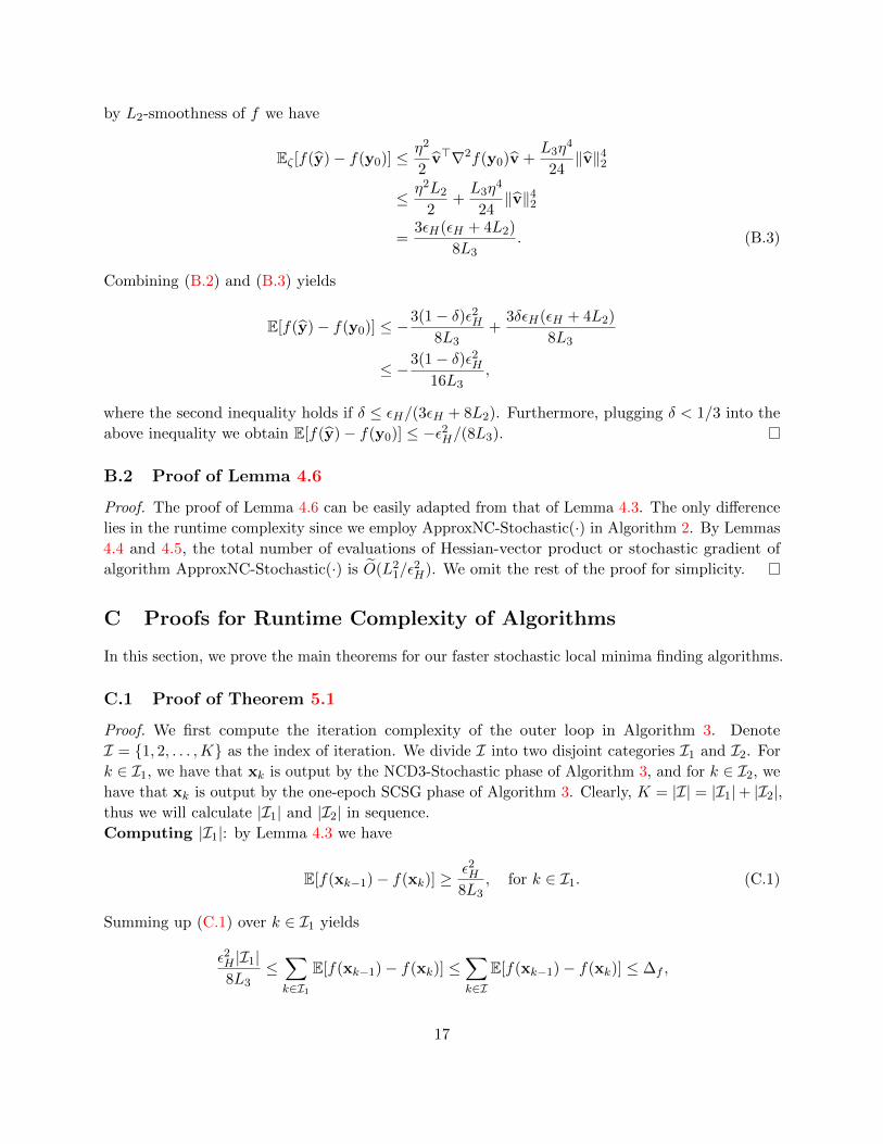
by L2-smoothness of f we have
Eζ [f(y)− f(y0)] ≤η2
2v>∇2f(y0)v +
L3η4
24‖v‖42
≤ η2L2
2+L3η
4
24‖v‖42
=3εH(εH + 4L2)
8L3. (B.3)
Combining (B.2) and (B.3) yields
E[f(y)− f(y0)] ≤ −3(1− δ)ε2H
8L3+
3δεH(εH + 4L2)
8L3
≤ −3(1− δ)ε2H16L3
,
where the second inequality holds if δ ≤ εH/(3εH + 8L2). Furthermore, plugging δ < 1/3 into the
above inequality we obtain E[f(y)− f(y0)] ≤ −ε2H/(8L3).
B.2 Proof of Lemma 4.6
Proof. The proof of Lemma 4.6 can be easily adapted from that of Lemma 4.3. The only difference
lies in the runtime complexity since we employ ApproxNC-Stochastic(·) in Algorithm 2. By Lemmas
4.4 and 4.5, the total number of evaluations of Hessian-vector product or stochastic gradient of
algorithm ApproxNC-Stochastic(·) is O(L21/ε
2H). We omit the rest of the proof for simplicity.
C Proofs for Runtime Complexity of Algorithms
In this section, we prove the main theorems for our faster stochastic local minima finding algorithms.
C.1 Proof of Theorem 5.1
Proof. We first compute the iteration complexity of the outer loop in Algorithm 3. Denote
I = {1, 2, . . . ,K} as the index of iteration. We divide I into two disjoint categories I1 and I2. For
k ∈ I1, we have that xk is output by the NCD3-Stochastic phase of Algorithm 3, and for k ∈ I2, we
have that xk is output by the one-epoch SCSG phase of Algorithm 3. Clearly, K = |I| = |I1|+ |I2|,thus we will calculate |I1| and |I2| in sequence.
Computing |I1|: by Lemma 4.3 we have
E[f(xk−1)− f(xk)] ≥ε2H8L3
, for k ∈ I1. (C.1)
Summing up (C.1) over k ∈ I1 yields
ε2H |I1|8L3
≤∑
k∈I1E[f(xk−1)− f(xk)] ≤
∑
k∈IE[f(xk−1)− f(xk)] ≤ ∆f ,
17

where the second inequality use the following fact by Corollary A.2
0 ≤ E[‖∇f(xk)‖22] ≤C1L1
n1/3E[f(xk−1)− f(xk)], for k ∈ I2, (C.2)
and C1 = 30 is a constant. Thus we further have
|I1| ≤8L3∆f
ε2H. (C.3)
Computing |I2|: to get the upper bound of |I2|, we further decompose I2 as I2 = I12 ∪ I22 , where
I12 = {k ∈ I2 | ‖gk‖2 > ε} and I22 = {k ∈ I2 | ‖gk‖2 ≤ ε}. Based on the definition, it is obvious
that I12 ∩ I22 = ∅ and |I2| = |I12 |+ |I22 |. According to update rules of Algorithm 3, if k ∈ I22 , then
Algorithm 3 will execute the NCD3-FiniteSum stage in the k-th iteration, which indicates that
|I22 | ≤ |I1|. Next we need to get the upper bound of |I12 |. Summing up (C.2) over k ∈ I12 yields
∑
k∈I12
E[‖∇f(xk)‖22] ≤C1L1
n1/3
∑
k∈I12
E[f(xk−1)− f(xk)]
≤ C1L1
n1/3
∑
k∈IE[f(xk−1)− f(xk)]
≤ C1L1∆f
n1/3,
where in the second inequality we use (C.1) and (C.2). Applying Markov’s inequality we obtain
with probability at least 2/3
∑
k∈I12
‖∇f(xk)‖22 ≤3C1L1∆f
n1/3.
Recall that for k ∈ I12 in Algorithm 3, we have ‖∇f(xk)‖2 > ε. We then obtain with probability at
least 2/3
|I12 | ≤3C1L1∆f
n1/3ε2. (C.4)
Computing Runtime: To calculate the total computation complexity in runtime, we need
to consider the runtime of stochastic gradient evaluations at each iteration of the algorithm.
Specifically, by Lemma 4.3 we know that each call of the NCD3-FiniteSum algorithm takes O((n+
n3/4√L1/εH)Th) runtime if FastPCA is used and O((n + n3/4
√L1/εH)Tg) runtime if Neon2 is
used. On the other hand, Corollary A.2 shows that the length of one epoch of SCSG algorithm is
O(n) which implies that the run time of one epoch of SCSG algorithm is O(nTg). Therefore, we
can compute the total time complexity of Algorithm 3 with Shifted-and-Inverted power method as
18

follows
|I1| · O((
n+n3/4L1/2
ε1/2H
)Th)
+ |I2| · O(nTg)
= |I1| · O((
n+n3/4L1/2
ε1/2H
)Th)
+ (|I12 |+ |I22 |) · O(nTg)
= |I1| · O((
n+n3/4L1/2
ε1/2H
)Th)
+ (|I12 |+ |I1|) · O(nTg),
where we used the fact that |I22 | ≤ |I1| in the last equation. Combining the upper bounds of |I1| in
(C.3) and |I12 | in (C.4) yields the following runtime complexity of Algorithm 3 with Shifted-and-
Inverted power method
O
(L3∆f
ε2H
)· O((
n+n3/4L1/2
ε1/2H
)Th)
+O
(L3∆f
ε2H+L1∆f
n1/3ε2
)· O(nTg)
= O
((L3∆fn
ε2H+L1/21 L3∆fn
3/4
ε5/2H
)Th +
(L1∆fn
2/3
ε2
)Tg),
and the runtime of Algorithm 3 with Neon2svrg is
O
((L3∆fn
ε2H+L1/21 L3∆fn
3/4
ε5/2H
+L1∆fn
2/3
ε2
)Tg),
which concludes our proof.
C.2 Proof of Theorem 5.5
Before we prove theoretical results for the stochastic setting, we lay down the following useful lemma
which states the concentration bound for sub-Gaussian random vectors.
Lemma C.1. (Ghadimi et al., 2016) Suppose the stochastic gradient ∇F (x; ξ) is sub-Gaussian
with parameter σ. Let ∇fS(x) = 1/|S|∑i∈S ∇F (x; ξi) be a subsampled gradient of f . If the sample
size |S| = 2σ2/ε2(1 +√
log(1/δ))2, then with probability 1− δ,
‖∇fS(x)−∇f(x)‖2 ≤ ε
holds for any x ∈ Rd.
Proof of Theorem 5.5. Similar to the proof of Theorem 5.1, we first calculate the outer loop iteration
complexity of Algorithm 4. Let I = {1, 2, . . . ,K} be the index of iteration. We use I1 and I2 to
denote the index set of iterates that are output by the NCD3-FiniteSum stage and SCSG stage
of Algorithm 4 respectively. It holds that K = |I| = |I1|+ |I2|. We will calculate |I1| and |I2| in
sequence.
Computing |I1|: note that |I1| is the number of iterations that Algorithm 4 calls NCD3-Stochastic
to find the negative curvature. Recall the result in Lemma 4.6, for k ∈ I1, one execution of the
19

NCD3-Stochastic stage can reduce the function value up to
E[f(xk−1)− f(xk)] ≥ε2H8L3
. (C.5)
To get the upper bound of |I1|, we also need to consider iterates output by One-epoch SCSG. By
Lemma A.3 it holds that
E[‖∇f(xk)‖22] ≤C1L1
B1/3E[f(xk−1)− f(xk)] +
C2σ2
B, for k ∈ I2, (C.6)
where C1 = 30 and C2 = 12 are absolute constants. For k ∈ I2, we further decompose I2 as
I2 = I12 ∪ I22 , where I12 = {k ∈ I2 | ‖gk‖2 > ε/2} and I22 = {k ∈ I2 | ‖gk‖2 ≤ ε/2}. It is easy to
see that I12 ∩ I22 = ∅ and |I2| = |I12 |+ |I22 |. In addition, according to the concentration result on
gk and ∇f(xk) in Lemma C.1, if the sample size B satisfies B = O(σ2/ε2 log(1/δ0)), then for any
k ∈ I12 , ‖∇f(xk)‖2 > ε/4 holds with probability at least 1 − δ0. For any k ∈ I22 , ‖∇f(xk)‖2 ≤ ε
holds with probability at least 1− δ0. According to (C.6), we can derive that for any k ∈ I12 ,
E[f(xk−1)− f(xk)] ≥B1/3
C1L1E[‖∇f(xk)‖22]−
C2σ2
C1L1B2/3, for k ∈ I12 . (C.7)
As for |I22 |, because for any k ∈ I22 , ‖gk‖2 ≤ ε/2, which will lead the algorithm to execute one step
of NCD3-Stochastic stage in the next iteration, i.e., k-th iteration. Thus it immediately implies
that |I22 | ≤ |I1|, and according to (C.6), we can also derive that
E[f(xk−1)− f(xk)] ≥ −C2σ
2
C1L1B2/3, for k ∈ I22 . (C.8)
Summing up (C.5) over k ∈ I1, (C.7) over k ∈ I12 , (C.8) over k ∈ I22 and combining the results
yields
∑
k∈IE[f(xk−1)− f(xk)] ≥
∑
k∈I1
ε2H8L3
+B1/3
C1L1
∑
k∈I12
E[‖∇f(xk)‖22]−∑
k∈I12
C2σ2
C1L1B2/3−∑
k∈I22
C2σ2
C1L1B2/3,
which immediately implies
|I1|ε2H8L3
+B1/3
C1L1
∑
k∈I12
E[‖∇f(xk)‖22] ≤ ∆f +∑
k∈I12
C2σ2
C1L1B2/3+∑
k∈I22
C2σ2
C1L1B2/3
≤ ∆f + |I12 |C2σ
2
C1L1B2/3+|I1|c2σ2C1L1B2/3
,
where the first inequality uses the fact that ∆f = f(x0)− infx f(x) and the second inequality is due
20
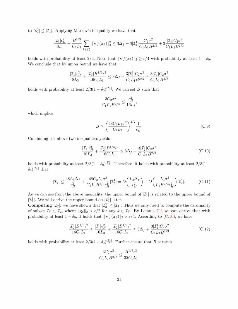
to |I22 | ≤ |I1|. Applying Markov’s inequality we have that
|I1|ε2H8L3
+B1/3
C1L1
∑
k∈I12
‖∇f(xk)‖22 ≤ 3∆f + 3|I12 |C2σ
2
C1L1B2/3+ 3|I1|C2σ
2
C1L1B2/3
holds with probability at least 2/3. Note that ‖∇f(xk)‖2 ≥ ε/4 with probability at least 1 − δ0.We conclude that by union bound we have that
|I1|ε2H8L3
+|I12 |B1/3ε2
16C1L1≤ 3∆f +
3|I12 |C2σ2
C1L1B2/3+
3|I1|C2σ2
C1L1B2/3
holds with probability at least 2/3(1− δ0)|I12 |. We can set B such that
3C2σ2
C1L1B2/3≤ ε2H
16L3,
which implies
B ≥(
48C2L3σ2
C1L1
)3/2 1
ε3H. (C.9)
Combining the above two inequalities yields
|I1|ε2H16L3
+|I12 |B1/3ε2
16C1L1≤ 3∆f +
3|I12 |C2σ2
C1L1B2/3(C.10)
holds with probability at least 2/3(1− δ0)|I12 |. Therefore, it holds with probability at least 2/3(1−δ0)|I12 | that
|I1| ≤48L3∆f
ε2H+
48C2L3σ2
C1L1B2/3ε2H|I12 | = O
(L3∆f
ε2H
)+ O
(L3σ
2
L1B2/3ε2H
)|I12 |. (C.11)
As we can see from the above inequality, the upper bound of |I1| is related to the upper bound of
|I12 |. We will derive the upper bound on |I12 | later.
Computing |I2|: we have shown that |I22 | ≤ |I1|. Thus we only need to compute the cardinality
of subset I12 ⊂ I2, where ‖gk‖2 > ε/2 for any k ∈ I12 . By Lemma C.1 we can derive that with
probability at least 1− δ0, it holds that ‖∇f(xk)‖2 > ε/4. According to (C.10), we have
|I12 |B1/3ε2
16C1L1≤ |I1|ε
2H
16L3+|I12 |B1/3ε2
16C1L1≤ 3∆f +
3|I12 |C2σ2
C1L1B2/3(C.12)
holds with probability at least 2/3(1− δ0)|I12 |. Further ensure that B satisfies
3C2σ2
C1L1B2/3≤ B1/3ε2
32C1L1,
21
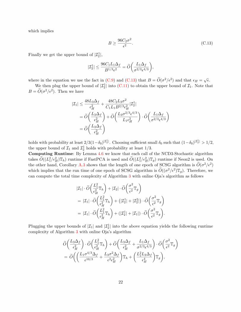
which implies
B ≥ 96C2σ2
ε2. (C.13)
Finally we get the upper bound of |I12 |,
|I12 | ≤96C1L1∆f
B1/3ε2= O
(L1∆f
σ2/3ε4/3
),
where in the equation we use the fact in (C.9) and (C.13) that B = O(σ2/ε2) and that εH =√ε.
We then plug the upper bound of |I12 | into (C.11) to obtain the upper bound of I1. Note that
B = O(σ2/ε2). Then we have
|I1| ≤48L3∆f
ε2H+
48C2L3σ2
C1L1B2/3ε2H|I12 |
= O
(L3∆f
ε2H
)+ O
(L3σ
2/3ε4/3
L1ε2H
)· O(
L1∆f
σ2/3ε4/3
)
= O
(L3∆f
ε2H
)
holds with probability at least 2/3(1−δ0)|I12 |. Choosing sufficient small δ0 such that (1−δ0)|I
12 | > 1/2,
the upper bound of I1 and I12 holds with probability at least 1/3.
Computing Runtime: By Lemma 4.6 we know that each call of the NCD3-Stochastic algorithm
takes O((L21/ε
2H)Th) runtime if FastPCA is used and O((L2
1/ε2H)Tg) runtime if Neon2 is used. On
the other hand, Corollary A.3 shows that the length of one epoch of SCSG algorithm is O(σ2/ε2)
which implies that the run time of one epoch of SCSG algorithm is O((σ2/ε2)Tg). Therefore, we
can compute the total time complexity of Algorithm 3 with online Oja’s algorithm as follows
|I1| · O(L21
ε2HTh)
+ |I2| · O(σ2
ε2Tg)
= |I1| · O(L21
ε2HTh)
+(|I12 |+ |I22 |
)· O(σ2
ε2Tg)
= |I1| · O(L21
ε2HTh)
+ (|I12 |+ |I1|) · O(σ2
ε2Tg).
Plugging the upper bounds of |I1| and |I12 | into the above equation yields the following runtime
complexity of Algorithm 3 with online Oja’s algorithm
O
(L3∆f
ε2H
)· O(L21
ε2HTh)
+ O
(L3∆f
ε2H+
L1∆f
σ2/3ε4/3
)· O(σ2
ε2Tg)
= O
((L1σ
4/3∆f
ε10/3+L3σ
2∆f
ε2ε2H
)Th +
(L21L3∆f
ε4H
)Tg),
22

and the runtime complexity of Algorithm 4 with Neon2online is
O
((L1σ
4/3∆f
ε10/3+L3σ
2∆f
ε2ε2H+L21L3∆f
ε4H
)Tg),
which concludes our proof.
References
Agarwal, N., Allen-Zhu, Z., Bullins, B., Hazan, E. and Ma, T. (2016). Finding approximate
local minima for nonconvex optimization in linear time. arXiv preprint arXiv:1611.01146 .
Allen-Zhu, Z. (2017). Natasha 2: Faster non-convex optimization than sgd. arXiv preprint
arXiv:1708.08694 .
Allen-Zhu, Z. and Hazan, E. (2016). Variance reduction for faster non-convex optimization. In
International Conference on Machine Learning.
Allen-Zhu, Z. and Li, Y. (2017a). Follow the compressed leader: Faster algorithms for matrix
multiplicative weight updates. arXiv preprint arXiv:1701.01722 .
Allen-Zhu, Z. and Li, Y. (2017b). Neon2: Finding local minima via first-order oracles. arXiv
preprint arXiv:1711.06673 .
Anandkumar, A. and Ge, R. (2016). Efficient approaches for escaping higher order saddle points
in non-convex optimization. In Conference on Learning Theory.
Carmon, Y. and Duchi, J. C. (2016). Gradient descent efficiently finds the cubic-regularized
non-convex newton step. arXiv preprint arXiv:1612.00547 .
Carmon, Y., Duchi, J. C., Hinder, O. and Sidford, A. (2016). Accelerated methods for
non-convex optimization. arXiv preprint arXiv:1611.00756 .
Carmon, Y., Hinder, O., Duchi, J. C. and Sidford, A. (2017). ” convex until proven
guilty”: Dimension-free acceleration of gradient descent on non-convex functions. arXiv preprint
arXiv:1705.02766 .
Choromanska, A., Henaff, M., Mathieu, M., Arous, G. B. and LeCun, Y. (2015). The loss
surfaces of multilayer networks. In Artificial Intelligence and Statistics.
Curtis, F. E., Robinson, D. P. and Samadi, M. (2017). A trust region algorithm with a
worst-case iteration complexity of\mathcal {O}(\epsilonˆ{-3/2}) for nonconvex optimization.
Mathematical Programming 162 1–32.
Dauphin, Y. N., Pascanu, R., Gulcehre, C., Cho, K., Ganguli, S. and Bengio, Y. (2014).
Identifying and attacking the saddle point problem in high-dimensional non-convex optimization.
In Advances in neural information processing systems.
23

Garber, D., Hazan, E., Jin, C., Musco, C., Netrapalli, P., Sidford, A. et al. (2016).
Faster eigenvector computation via shift-and-invert preconditioning. In International Conference
on Machine Learning.
Ge, R., Huang, F., Jin, C. and Yuan, Y. (2015). Escaping from saddle pointsonline stochastic
gradient for tensor decomposition. In Conference on Learning Theory.
Ghadimi, S., Lan, G. and Zhang, H. (2016). Mini-batch stochastic approximation methods for
nonconvex stochastic composite optimization. Mathematical Programming 155 267–305.
Hillar, C. J. and Lim, L.-H. (2013). Most tensor problems are np-hard. Journal of the ACM
(JACM) 60 45.
Jin, C., Ge, R., Netrapalli, P., Kakade, S. M. and Jordan, M. I. (2017a). How to escape
saddle points efficiently. arXiv preprint arXiv:1703.00887 .
Jin, C., Netrapalli, P. and Jordan, M. I. (2017b). Accelerated gradient descent escapes saddle
points faster than gradient descent. arXiv preprint arXiv:1711.10456 .
Kohler, J. M. and Lucchi, A. (2017). Sub-sampled cubic regularization for non-convex optimiza-
tion. arXiv preprint arXiv:1705.05933 .
Kuczynski, J. and Wozniakowski, H. (1992). Estimating the largest eigenvalue by the power
and lanczos algorithms with a random start. SIAM journal on matrix analysis and applications
13 1094–1122.
LeCun, Y., Bengio, Y. and Hinton, G. (2015). Deep learning. Nature 521 436–444.
Lei, L., Ju, C., Chen, J. and Jordan, M. I. (2017). Nonconvex finite-sum optimization via scsg
methods. arXiv preprint arXiv:1706.09156 .
Levy, K. Y. (2016). The power of normalization: Faster evasion of saddle points. arXiv preprint
arXiv:1611.04831 .
More, J. J. and Sorensen, D. C. (1979). On the use of directions of negative curvature in a
modified newton method. Mathematical Programming 16 1–20.
Nesterov, Y. and Polyak, B. T. (2006). Cubic regularization of newton method and its global
performance. Mathematical Programming 108 177–205.
Reddi, S. J., Hefny, A., Sra, S., Poczos, B. and Smola, A. (2016). Stochastic variance
reduction for nonconvex optimization. In International conference on machine learning.
Reddi, S. J., Zaheer, M., Sra, S., Poczos, B., Bach, F., Salakhutdinov, R. and Smola,
A. J. (2017). A generic approach for escaping saddle points. arXiv preprint arXiv:1709.01434 .
Tripuraneni, N., Stern, M., Jin, C., Regier, J. and Jordan, M. I. (2017). Stochastic cubic
regularization for fast nonconvex optimization. arXiv preprint arXiv:1711.02838 .
24

Vershynin, R. (2010). Introduction to the non-asymptotic analysis of random matrices. arXiv
preprint arXiv:1011.3027 .
Xu, P., Roosta-Khorasani, F. and Mahoney, M. W. (2017). Newton-type methods for
non-convex optimization under inexact hessian information. arXiv preprint arXiv:1708.07164 .
Xu, Y. and Yang, T. (2017). First-order stochastic algorithms for escaping from saddle points in
almost linear time. arXiv preprint arXiv:1711.01944 .
Yu, Y., Zou, D. and Gu, Q. (2017). Saving gradient and negative curvature computations:
Finding local minima more efficiently. arXiv preprint arXiv:1712.03950 .
25