Embed Size (px)
Citation preview

• Table of
Contents
• Index
• Reviews
• Examples
• Reader
Reviews
• Errata
Mastering Algorithms with C
By Kyle Loudon
Publisher: O'Reilly
Pub Date: August 1999
ISBN: 1-56592-453-3
Pages: 560
This book offers robust solutions for everyday programming tasks,providing all the necessary information to understand and use commonprogramming techniques. It includes implementations and real-worldexamples of each data structure in the text and full source code on theaccompanying website (http://examples.oreilly.com/masteralgoc/).Intended for anyone with a basic understanding of the C language.

• Table of
Contents
• Index
• Reviews
• Examples
• Reader
Reviews
• Errata
Mastering Algorithms with C
By Kyle Loudon
Publisher: O'Reilly
Pub Date: August 1999
ISBN: 1-56592-453-3
Pages: 560
Copyright
Preface
Organization
Key Features
About the Code
Conventions
How to Contact Us
Acknowledgments
Part I: Preliminaries
Chapter 1. Introduction
Section 1.1. An Introduction to Data Structures
Section 1.2. An Introduction to Algorithms
Section 1.3. A Bit About Software Engineering
Section 1.4. How to Use This Book
Chapter 2. Pointer Manipulation
Section 2.1. Pointer Fundamentals
Section 2.2. Storage Allocation
Section 2.3. Aggregates and Pointer Arithmetic
Section 2.4. Pointers as Parameters to Functions
Section 2.5. Generic Pointers and Casts
Section 2.6. Function Pointers
Section 2.7. Questions and Answers
Section 2.8. Related Topics
Chapter 3. Recursion
Section 3.1. Basic Recursion
Section 3.2. Tail Recursion
Section 3.3. Questions and Answers
Section 3.4. Related Topics

Chapter 4. Analysis of Algorithms
Section 4.1. Worst-Case Analysis
Section 4.2. O-Notation
Section 4.3. Computational Complexity
Section 4.4. Analysis Example: Insertion Sort
Section 4.5. Questions and Answers
Section 4.6. Related Topics
Part II: Data Structures
Chapter 5. Linked Lists
Section 5.1. Description of Linked Lists
Section 5.2. Interface for Linked Lists
Section 5.3. Implementation and Analysis of Linked Lists
Section 5.4. Linked List Example: Frame Management
Section 5.5. Description of Doubly-Linked Lists
Section 5.6. Interface for Doubly-Linked Lists
Section 5.7. Implementation and Analysis of Doubly Linked Lists
Section 5.8. Description of Circular Lists
Section 5.9. Interface for Circular Lists
Section 5.10. Implementation and Analysis of Circular Lists
Section 5.11. Circular List Example: Second-Chance Page Replacement
Section 5.12. Questions and Answers
Section 5.13. Related Topics
Chapter 6. Stacks and Queues
Section 6.1. Description of Stacks
Section 6.2. Interface for Stacks
Section 6.3. Implementation and Analysis of Stacks
Section 6.4. Description of Queues
Section 6.5. Interface for Queues
Section 6.6. Implementation and Analysis of Queues
Section 6.7. Queue Example: Event Handling
Section 6.8. Questions and Answers
Section 6.9. Related Topics
Chapter 7. Sets
Section 7.1. Description of Sets
Section 7.2. Interface for Sets
Section 7.3. Implementation and Analysis of Sets
Section 7.4. Set Example: Set Covering
Section 7.5. Questions and Answers
Section 7.6. Related Topics
Chapter 8. Hash Tables
Section 8.1. Description of Chained Hash Tables
Section 8.2. Interface for Chained Hash Tables
Section 8.3. Implementation and Analysis of Chained Hash Tables
Section 8.4. Chained Hash Table Example: Symbol Tables
Section 8.5. Description of Open-Addressed Hash Tables
Section 8.6. Interface for Open-Addressed Hash Tables
Section 8.7. Implementation and Analysisof Open Addressed Hash Tables

Section 8.8. Questions and Answers
Section 8.9. Related Topics
Chapter 9. Trees
Section 9.1. Description of Binary Trees
Section 9.2. Interface for Binary Trees
Section 9.3. Implementation and Analysis of Binary Trees
Section 9.4. Binary Tree Example: Expression Processing
Section 9.5. Description of Binary Search Trees
Section 9.6. Interface for Binary Search Trees
Section 9.7. Implementation and Analysis of Binary Search Trees
Section 9.8. Questions and Answers
Section 9.9. Related Topics
Chapter 10. Heaps and Priority Queues
Section 10.1. Description of Heaps
Section 10.2. Interface for Heaps
Section 10.3. Implementation and Analysis of Heaps
Section 10.4. Description of Priority Queues
Section 10.5. Interface for Priority Queues
Section 10.6. Implementation and Analysis of Priority Queues
Section 10.7. Priority Queue Example: Parcel Sorting
Section 10.8. Questions and Answers
Section 10.9. Related Topics
Chapter 11. Graphs
Section 11.1. Description of Graphs
Section 11.2. Interface for Graphs
Section 11.3. Implementation and Analysis of Graphs
Section 11.4. Graph Example: Counting Network Hops
Section 11.5. Graph Example: Topological Sorting
Section 11.6. Questions and Answers
Section 11.7. Related Topics
Part III: Algorithms
Chapter 12. Sorting and Searching
Section 12.1. Description of Insertion Sort
Section 12.2. Interface for Insertion Sort
Section 12.3. Implementation and Analysis of Insertion Sort
Section 12.4. Description of Quicksort
Section 12.5. Interface for Quicksort
Section 12.6. Implementation and Analysis of Quicksort
Section 12.7. Quicksort Example: Directory Listings
Section 12.8. Description of Merge Sort
Section 12.9. Interface for Merge Sort
Section 12.10. Implementation and Analysis of Merge Sort
Section 12.11. Description of Counting Sort
Section 12.12. Interface for Counting Sort
Section 12.13. Implementation and Analysis of Counting Sort
Section 12.14. Description of Radix Sort
Section 12.15. Interface for Radix Sort

Section 12.16. Implementation and Analysis of Radix Sort
Section 12.17. Description of Binary Search
Section 12.18. Interface for Binary Search
Section 12.19. Implementation and Analysis of Binary Search
Section 12.20. Binary Search Example: Spell Checking
Section 12.21. Questions and Answers
Section 12.22. Related Topics
Chapter 13. Numerical Methods
Section 13.1. Description of Polynomial Interpolation
Section 13.2. Interface for Polynomial Interpolation
Section 13.3. Implementation and Analysis of Polynomial Interpolation
Section 13.4. Description of Least-Squares Estimation
Section 13.5. Interface for Least-Squares Estimation
Section 13.6. Implementation and Analysis of Least-Squares Estimation
Section 13.7. Description of the Solution of Equations
Section 13.8. Interface for the Solution of Equations
Section 13.9. Implementation and Analysis of the Solution of Equations
Section 13.10. Questions and Answers
Section 13.11. Related Topics
Chapter 14. Data Compression
Section 14.1. Description of Bit Operations
Section 14.2. Interface for Bit Operations
Section 14.3. Implementation and Analysis of Bit Operations
Section 14.4. Description of Huffman Coding
Section 14.5. Interface for Huffman Coding
Section 14.6. Implementation and Analysis of Huffman Coding
Section 14.7. Huffman Coding Example: Optimized Networking
Section 14.8. Description of LZ77
Section 14.9. Interface for LZ77
Section 14.10. Implementation and Analysis of LZ77
Section 14.11. Questions and Answers
Section 14.12. Related Topics
Chapter 15. Data Encryption
Section 15.1. Description of DES
Section 15.2. Interface for DES
Section 15.3. Implementation and Analysis of DES
Section 15.4. DES Example: Block Cipher Modes
Section 15.5. Description of RSA
Section 15.6. Interface for RSA
Section 15.7. Implementation and Analysis of RSA
Section 15.8. Questions and Answers
Section 15.9. Related Topics
Chapter 16. Graph Algorithms
Section 16.1. Description of Minimum Spanning Trees
Section 16.2. Interface for Minimum Spanning Trees
Section 16.3. Implementation and Analysis of Minimum Spanning Trees
Section 16.4. Description of Shortest Paths
Section 16.5. Interface for Shortest Paths

Section 16.6. Implementation and Analysis of Shortest Paths
Section 16.7. Shortest Paths Example: Routing Tables
Section 16.8. Description of the Traveling-Salesman Problem
Section 16.9. Interface for the Traveling-Salesman Problem
Section 16.10. Implementation and Analysis of the Traveling-Salesman Problem
Section 16.11. Questions and Answers
Section 16.12. Related Topics
Chapter 17. Geometric Algorithms
Section 17.1. Description of Testing Whether Line Segments Intersect
Section 17.2. Interface for Testing Whether Line Segments Intersect
Section 17.3. Implementation and Analysis of Testing Whether Line Segments Intersect
Section 17.4. Description of Convex Hulls
Section 17.5. Interface for Convex Hulls
Section 17.6. Implementation and Analysis of Convex Hulls
Section 17.7. Description of Arc Length on Spherical Surfaces
Section 17.8. Interface for Arc Length on Spherical Surfaces
Section 17.9. Implementation and Analysis of Arc Length on Spherical Surfaces
Section 17.10. Arc Length Example: Approximating Distances on Earth
Section 17.11. Questions and Answers
Section 17.12. Related Topics
Colophon
Index
Top

Mastering Algorithms with CBy Kyle Loudon
Slots : 1
Table of Contents
Content
Copyright © 1999 O'Reilly & Associates, Inc. All rights reserved.
Printed in the United States of America.
Published by O'Reilly & Associates, Inc., 1005 Gravenstein Highway North, Sebastopol, CA 95472.
O'Reilly & Associates books may be purchased for educational, business, or sales promotional use.Online editions are also available for most titles (safari.oreilly.com). For more information, contactour corporate/institutional sales department: (800) 998-9938 or [email protected].
Nutshell Handbook, the Nutshell Handbook logo, and the O'Reilly logo are registered trademarks ofO'Reilly & Associates, Inc. Many of the designations used by manufacturers and sellers to distinguishtheir products are claimed as trademarks. Where those designations appear in this book, and O'Reilly& Associates, Inc. was aware of a trademark claim, the designations have been printed in caps orinitial caps. The association between the image of sea horses and the topic of algorithms with C is atrademark of O'Reilly & Associates, Inc.
While every precaution has been taken in the preparation of this book, the publisher assumes noresponsibility for errors or omissions, or for damages resulting from the use of the informationcontained herein.
Top

Mastering Algorithms with CBy Kyle Loudon
Slots : 1
Table of Contents
Content
PrefaceWhen I first thought about writing this book, I immediately thought of O'Reilly & Associates to publishit. They were the first publisher I contacted, and the one I most wanted to work with because of theirtradition of books covering "just the facts." This approach is not what one normally thinks of inconnection with books on data structures and algorithms. When one studies data structures andalgorithms, normally there is a fair amount of time spent on proving their correctness rigorously.Consequently, many books on this subject have an academic feel about them, and real details suchas implementation and application are left to be resolved elsewhere. This book covers how and whycertain data structures and algorithms work, real applications that use them (including manyexamples), and their implementation. Mathematical rigor appears only to the extent necessary inexplanations.
Naturally, I was very happy that O'Reilly & Associates saw value in a book that covered this aspect ofthe subject. This preface contains some of the reasons I think you will find this book valuable as well.It also covers certain aspects of the code in the book, defines a few conventions, and gratefullyacknowledges the people who played a part in the book's creation.
Top

Mastering Algorithms with CBy Kyle Loudon
Slots : 1
Table of Contents
Preface
Content
Organization
This book is divided into three parts. The first part consists of introductory material that is usefulwhen working in the rest of the book. The second part presents a number of data structuresconsidered fundamental in the field of computer science. The third part presents an assortment ofalgorithms for solving common problems. Each of these parts is described in more detail in thefollowing sections, including a summary of the chapters each part contains.
Part I
Part I contains Chapter 1 through Chapter 4. Chapter 1, introduces the concepts of data structuresand algorithms and presents reasons for using them. It also presents a few topics in softwareengineering, which are applied throughout the rest of the book. Chapter 2 discusses a number oftopics on pointers. Pointers appear a great deal in this book, so this chapter serves as a refresher onthe subject. Chapter 3 covers recursion, a popular technique used with many data structures andalgorithms. Chapter 4 presents the analysis of algorithms. The techniques in this chapter are used toanalyze algorithms throughout the book.
Part II
Part II contains Chapter 5 through Chapter 11. Chapter 5 presents various forms of linked lists,including singly-linked lists, doubly-linked lists, and circular lists. Chapter 6 presents stacks andqueues, data structures for sorting and returning data on a last-in, first-out and first-in, first-outorder respectively. Chapter 7 presents sets and the fundamental mathematics describing sets.Chapter 8 presents chained and open-addressed hash tables, including material on how to select agood hash function and how to resolve collisions. Chapter 9 presents binary and AVL trees. Chapter 9also discusses various methods of tree traversal. Chapter 10 presents heaps and priority queues,data structures that help to quickly determine the largest or smallest element in a set of data.Chapter 11 presents graphs and two fundamental algorithms from which many graph algorithms arederived: breadth-first and depth-first search.
Part III

Part III, contains Chapter 12 through Chapter 17. Chapter 12 covers various algorithms for sorting,including insertion sort, quicksort, merge sort, counting sort, and radix sort. Chapter 12 also presentsbinary search. Chapter 13 covers numerical methods, including algorithms for polynomialinterpolation, least-squares estimation, and the solution of equations using Newton's method.Chapter 14 presents algorithms for data compression, including Huffman coding and LZ77. Chapter15 discusses algorithms for DES and RSA encryption. Chapter 16 covers graph algorithms, includingPrim's algorithm for minimum spanning trees, Dijkstra's algorithm for shortest paths, and analgorithm for solving the traveling-salesman problem. Chapter 17 presents geometric algorithms,including methods for testing whether line segments intersect, computing convex hulls, andcomputing arc lengths on spherical surfaces.
Top

Mastering Algorithms with CBy Kyle Loudon
Slots : 1
Table of Contents
Preface
Content
Key Features
There are a number of special features that I believe together make this book a unique approach tocovering the subject of data structures and algorithms:
Consistent format for every chapter
Every chapter (excluding those in the first part of the book) follows a consistent format. Thisformat allows most of the book to be read as a textbook or a reference, whichever is needed atthe moment.
Clearly identified topics and applications
Each chapter (except Chapter 1) begins with a brief introduction, followed by a list of clearlyidentified topics and their relevance to real applications.
Analyses of every operation, algorithm, and example
An analysis is provided for every operation of abstract datatypes, every algorithm in thealgorithms chapters, and every example throughout the book. Each analysis uses thetechniques presented in Chapter 4.
Real examples, not just trivial exercises
All examples are from real applications, not just trivial exercises. Examples like these areexciting and teach more than just the topic being demonstrated.
Real implementations using real code
All implementations are written in C, not pseudocode. The benefit of this is that whenimplementing many data structures and algorithms, there are considerable details pseudocodedoes not address.
Questions and answers for further thought
At the end of each chapter (except Chapter 1), there is a series of questions along with theiranswers. These emphasize important ideas from the chapter and touch on additional topics.
Lists of related topics for further exploration
At the end of each chapter (except Chapter 1), there is a list of related topics for furtherexploration. Each topic is presented with a brief description.
Numerous cross references and call-outs

Cross references and call-outs mark topics mentioned in one place that are introducedelsewhere. Thus, it is easy to locate additional information.
Insightful organization and application of topics
Many of the data structures or algorithms in one chapter use data structures and algorithmspresented elsewhere in the book. Thus, they serve as examples of how to use other datastructures and algorithms themselves. All dependencies are carefully marked with a crossreference or call-out.
Coverage of fundamental topics, plus more
This book covers the fundamental data structures and algorithms of computer science. It alsocovers several topics not normally addressed in books on the subject. These include numericalmethods, data compression (in more detail), data encryption, and geometric algorithms.
Top
Mastering Algorithms with CBy Kyle Loudon
Slots : 1
Table of Contents
Preface
Content
About the Code
All implementations in this book are in C. C was chosen because it is still the most general-purposelanguage in use today. It is also one of the best languages in which to explore the details of datastructures and algorithms while still working at a fairly high level. It may be helpful to note a fewthings about the code in this book.
All code focuses on pedagogy first
There is also a focus on efficiency, but the primary purpose of all code is to teach the topic itaddresses in a clear manner.
All code has been fully tested on four platforms
The platforms used for testing were HP-UX 10.20, SunOs 5.6, Red Hat Linux 5.1, andDOS/Windows NT/95/98. See the readme file on the accompanying websitehttp://examples.oreilly.com/masteralgoc/) for additional information.
Headers document all public interfaces
Every implementation includes a header that documents the public interface. Most headers areshown in this book. However, headers that contain only prototypes are not. (For instance,Example 12.1 includes sort.h, but this header is not shown because it contains only prototypesto various sorting functions.)
Static functions are used for private functions
Static functions have file scope, so this fact is used to keep private functions private. Functionsspecific to a data structure or algorithm's implementation are thus kept out of its publicinterface.
Naming conventions are applied throughout the code
Defined constants appear entirely in uppercase. Datatypes and global variables begin with anuppercase character. Local variables begin with a lowercase character. Operations of abstractdatatypes begin with the name of the type in lowercase, followed by an underscore, then thename of the operation in lowercase.
All code contains numerous comments
All comments are designed to let developers follow the logic of the code without reading muchof the code itself. This is useful when trying to make connections between the code andexplanations in the text.

Structures have typedefs as well as names themselves
The name of the structure is always the name in the typedef followed by an underscore.Naming the structure itself is necessary for self-referential structures like the one used forlinked list elements (see Chapter 5). This approach is applied everywhere for consistency.
All void functions contain explicit returns
Although not required, this helps quickly identify where a void function returns rather thanhaving to match up braces.
Top

Mastering Algorithms with CBy Kyle Loudon
Slots : 1
Table of Contents
Preface
Content
Conventions
Most of the conventions used in this book should be recognizable to those who work with computersto any extent. However, a few require some explanation.
Bold italic
Nonintrinsic mathematical functions and mathematical variables appear in this font.Constant width italic
Variables from programs, names of datatypes (such as structure names), and definedconstants appear in this font.
Italic
Commands (as they would be typed in at a terminal), names of files and paths, operations ofabstract datatypes, and other functions from programs appear in this font.
lg x
This notation is used to represent the base-2 logarithm of x, log2 x. This is the notation usedcommonly in computer science when discussing algorithms; therefore, it is used in this book.
Top

Mastering Algorithms with CBy Kyle Loudon
Slots : 1
Table of Contents
Preface
Content
How to Contact Us
We have tested and verified the information in this book to the best of our ability, but you may findthat features have changed (or even that we have made mistakes!). Please let us know about anyerrors you find, as well as your suggestions for future editions, by writing to:
O'Reilly & Associates, Inc.1005 Gravenstein Highway NorthSebastopol, CA 954721-800-998-9938 (in the U.S. or Canada)1-707-829-0515 (international/local)1-707-829-0104 (FAX)
You can also send us messages electronically. To be put on the mailing list or request a catalog, sendemail to:
To ask technical questions or comment on the book, send email to:
We have a web site for the book, where we'll list examples, errata, and any plans for future editions.You can access this page at:
http://www.oreilly.com/catalog/masteralgoc/
For more information about this book and others, see the O'Reilly web site:
http://www.oreilly.com/
Top

Mastering Algorithms with CBy Kyle Loudon
Slots : 1
Table of Contents
Preface
Content
Acknowledgments
The experience of writing a book is not without its ups and downs. On the one hand, there isexcitement, but there is also exhaustion. It is only with the support of others that one can trulydelight in its pleasures and overcome its perils. There are many people I would like to thank.
First, I thank Andy Oram, my editor at O'Reilly & Associates, whose assistance has been exceptionalin every way. I thank Andy especially for his continual patience and support. In addition, I would liketo thank Tim O'Reilly and Andy together for their interest in this project when it first began. Otherindividuals I gratefully acknowledge at O'Reilly & Associates are Rob Romano for drafting thetechnical illustrations, and Lenny Muellner and Mike Sierra, members of the tools group, who werealways quick to reply to my questions. I thank Jeffrey Liggett for his swift and detailed work duringthe production process. In addition, I would like to thank the many others I did not correspond withdirectly at O'Reilly & Associates but who played no less a part in the production of this book. Thankyou, everyone.
Several individuals gave me a great deal of feedback in the form of reviews. I owe a special debt ofgratitude to Bill Greene of Intel Corporation for his enthusiasm and voluntary support in reviewingnumerous chapters throughout the writing process. I also would like to thank Alan Solis of Com21 forreviewing several chapters. I thank Alan, in addition, for the considerable knowledge he has impartedto me over the years at our weekly lunches. I thank Stephen Friedl for his meticulous review of thecompleted manuscript. I thank Shaun Flisakowski for the review she provided at the manuscript'scompletion as well. In addition, I gratefully acknowledge those who looked over chapters with mefrom time to time and with whom I discussed material for the book on an ongoing basis.
Many individuals gave me support in countless other ways. First, I would like to thank Jeff Moore, mycolleague and friend at Jeppesen, whose integrity and pursuit of knowledge constantly inspire me.During our frequent conversations, Jeff was kind enough to indulge me often by discussing topics inthe book. Thank you, Jeff. I would also like to thank Ken Sunseri, my manager at Jeppesen, forcreating an environment at work in which a project like this was possible. Furthermore, I warmlythank all of my friends and family for their love and support throughout my writing. In particular, Ithank Marc Loudon for answering so many of my questions. I thank Marc and Judy Loudon togetherfor their constant encouragement. I thank Shala Hruska for her patience, understanding, and supportat the project's end, which seemed to last so long.
Finally, I would like to thank Robert Foerster, my teacher, for the experiences we shared on a 16KTRS-80 in 1981. I still recall those times fondly. They made a wonderful difference in my life. For

giving me my start with computers, I dedicate this book to you with affection.
Top

Mastering Algorithms with CBy Kyle Loudon
Slots : 1
Table of Contents
Content
Part I: PreliminariesThis part of the book contains four chapters of introductory material. Chapter 1, introduces theconcepts of data structures and algorithms and presents reasons for using them. It alsopresents a few topics in software engineering that are applied throughout the rest of the book.Chapter 2, presents a number of topics on pointers. Pointers appear a great deal in this book,so this chapter serves as a refresher on the subject. Chapter 3, presents recursion, a populartechnique used with many data structures and algorithms. Chapter 4, describes how to analyzealgorithms. The techniques in this chapter are used to analyze algorithms throughout the book.
Top

Mastering Algorithms with CBy Kyle Loudon
Slots : 1
Table of Contents
Part I: Preliminaries
Content
Chapter 1. IntroductionWhen I was 12, my brother and I studied piano. Each week we would make a trip to our teacher'shouse; while one of us had our lesson, the other would wait in her parlor. Fortunately, she alwayshad a few games arranged on a coffee table to help us pass the time while waiting. One game Iremember consisted of a series of pegs on a small piece of wood. Little did I know it, but the gamewould prove to be an early introduction to data structures and algorithms.
The game was played as follows. All of the pegs were white, except for one, which was blue. Tobegin, one of the white pegs was removed to create an empty hole. Then, by jumping pegs andremoving them much like in checkers, the game continued until a single peg was left, or theremaining pegs were scattered about the board in such a way that no more jumps could be made.The object of the game was to jump pegs so that the blue peg would end up as the last peg and inthe center. According to the game's legend, this qualified the player as a "genius." Additional levels ofintellect were prescribed for other outcomes. As for me, I felt satisfied just getting through a gamewithout our teacher's kitten, Clara, pouncing unexpectedly from around the sofa to sink her clawsinto my right shoe. I suppose being satisfied with this outcome indicated that I simply possessed"common sense."
I remember playing the game thinking that certainly a deterministic approach could be found to getthe blue peg to end up in the center every time. What I was looking for was an algorithm. Algorithmsare well-defined procedures for solving problems. It was not until a number of years later that Iactually implemented an algorithm for solving the peg problem. I decided to solve it in LISP during anartificial intelligence class in college. To solve the problem, I represented information about the gamein various data structures. Data structures are conceptual organizations of information. They go handin hand with algorithms because many algorithms rely on them for efficiency.
Often, people deal with information in fairly loose forms, such as pegs on a board, notes in anotebook, or drawings in a portfolio. However, to process information with a computer, theinformation needs to be more formally organized. In addition, it is helpful to have a precise plan forexactly what to do with it. Data structures and algorithms help us with this. Simply stated, they helpus develop programs that are, in a word, elegant. As developers of software, it is important toremember that we must be more than just proficient with programming languages and developmenttools; developing elegant software is a matter of craftsmanship. A good understanding of datastructures and algorithms is an important part of becoming such a craftsman.

Top

Mastering Algorithms with CBy Kyle Loudon
Slots : 1
Table of Contents
Chapter 1. Introduction
Content
1.1 An Introduction to Data Structures
Data comes in all shapes and sizes, but often it can be organized in the same way. For example,consider a list of things to do, a list of ingredients in a recipe, or a reading list for a class. Althougheach contains a different type of data, they all contain data organized in a similar way: a list. A list isone simple example of a data structure. Of course, there are many other common ways to organizedata as well. In computing, some of the most common organizations are linked lists, stacks, queues,sets, hash tables, trees, heaps, priority queues, and graphs, all of which are discussed in this book.Three reasons for using data structures are efficiency, abstraction, and reusability.
Efficiency
Data structures organize data in ways that make algorithms more efficient. For example,consider some of the ways we can organize data for searching it. One simplistic approach is toplace the data in an array and search the data by traversing element by element until thedesired element is found. However, this method is inefficient because in many cases we end uptraversing every element. By using another type of data structure, such as a hash table (seeChapter 8) or a binary tree (see Chapter 9) we can search the data considerably faster.
Abstraction
Data structures provide a more understandable way to look at data; thus, they offer a level ofabstraction in solving problems. For example, by storing data in a stack (see Chapter 6), wecan focus on things that we do with stacks, such as pushing and popping elements, rather thanthe details of how to implement each operation. In other words, data structures let us talkabout programs in a less programmatic way.
Reusability
Data structures are reusable because they tend to be modular and context-free. They aremodular because each has a prescribed interface through which access to data stored in thedata structure is restricted. That is, we access the data using only those operations theinterface defines. Data structures are context-free because they can be used with any type ofdata and in a variety of situations or contexts. In C, we make a data structure store data ofany type by using void pointers to the data rather than by maintaining private copies of thedata in the data structure itself.
When one thinks of data structures, one normally thinks of certain actions, or operations, one wouldlike to perform with them as well. For example, with a list, we might naturally like to insert, remove,traverse, and count elements. A data structure together with basic operations like these is called an

abstract datatype. The operations of an abstract datatype constitute its public interface. The publicinterface of an abstract datatype defines exactly what we are allowed to do with it. Establishing andadhering to an abstract datatype's interface is essential because this lets us better manage aprogram's data, which inevitably makes a program more understandable and maintainable.
Top

Mastering Algorithms with CBy Kyle Loudon
Slots : 1
Table of Contents
Chapter 1. Introduction
Content
1.2 An Introduction to Algorithms
Algorithms are well-defined procedures for solving problems. In computing, algorithms are essentialbecause they serve as the systematic procedures that computers require. A good algorithm is likeusing the right tool in a workshop. It does the job with the right amount of effort. Using the wrongalgorithm or one that is not clearly defined is like cutting a piece of paper with a table saw, or tryingto cut a piece of plywood with a pair of scissors: although the job may get done, you have to wonderhow effective you were in completing it. As with data structures, three reasons for using formalalgorithms are efficiency, abstraction, and reusability.
Efficiency
Because certain types of problems occur often in computing, researchers have found efficientways of solving them over time. For example, imagine trying to sort a number of entries in anindex for a book. Since sorting is a common task that is performed often, it is not surprisingthat there are many efficient algorithms for doing this. We explore some of these in Chapter12.
Abstraction
Algorithms provide a level of abstraction in solving problems because many seeminglycomplicated problems can be distilled into simpler ones for which well-known algorithms exist.Once we see a more complicated problem in a simpler light, we can think of the simplerproblem as just an abstraction of the more complicated one. For example, imagine trying tofind the shortest way to route a packet between two gateways in an internet. Once we realizethat this problem is just a variation of the more general single-pair shortest-paths problem(see Chapter 16), we can approach it in terms of this generalization.
Reusability
Algorithms are often reusable in many different situations. Since many well- known algorithmssolve problems that are generalizations of more complicated ones, and since many complicatedproblems can be distilled into simpler ones, an efficient means of solving certain simplerproblems potentially lets us solve many others.
1.2.1 General Approaches in Algorithm Design
In a broad sense, many algorithms approach problems in the same way. Thus, it is often convenient

to classify them based on the approach they employ. One reason to classify algorithms in this way isthat often we can gain some insight about an algorithm if we understand its general approach. Thiscan also give us ideas about how to look at similar problems for which we do not know algorithms. Ofcourse, some algorithms defy classification, whereas others are based on a combination ofapproaches. This section presents some common approaches.
1.2.1.1 Randomized algorithms
Randomized algorithms rely on the statistical properties of random numbers. One example of arandomized algorithm is quicksort (see Chapter 12).
Quicksort works as follows. Imagine sorting a pile of canceled checks by hand. We begin with anunsorted pile that we partition in two. In one pile we place all checks numbered less than or equal towhat we think may be the median value, and in the other pile we place the checks numbered greaterthan this. Once we have the two piles, we divide each of them in the same manner and repeat theprocess until we end up with one check in every pile. At this point the checks are sorted.
In order to achieve good performance, quicksort relies on the fact that each time we partition thechecks, we end up with two partitions that are nearly equal in size. To accomplish this, ideally weneed to look up the median value of the check numbers before partitioning the checks. However,since determining the median requires scanning all of the checks, we do not do this. Instead, werandomly select a check around which to partition. Quicksort performs well on average because thenormal distribution of random numbers leads to relatively balanced partitioning overall.
1.2.1.2 Divide-and-conquer algorithms
Divide-and-conquer algorithms revolve around three steps: divide, conquer, and combine. In thedivide step, we divide the data into smaller, more manageable pieces. In the conquer step, weprocess each division by performing some operation on it. In the combine step, we recombine theprocessed divisions. One example of a divide-and-conquer algorithm is merge sort (see Chapter 12).
Merge sort works as follows. As before, imagine sorting a pile of canceled checks by hand. We beginwith an unsorted pile that we divide in half. Next, we divide each of the resulting two piles in half andcontinue this process until we end up with one check in every pile. Once all piles contain a singlecheck, we merge the piles two by two so that each new pile is a sorted combination of the two thatwere merged. Merging continues until we end up with one big pile again, at which point the checksare sorted.
In terms of the three steps common to all divide-and-conquer algorithms, merge sort can bedescribed as follows. First, in the divide step, divide the data in half. Next, in the conquer step, sortthe two divisions by recursively applying merge sort to them. Last, in the combine step, merge thetwo divisions into a single sorted set.
1.2.1.3 Dynamic-programming solutions
Dynamic-programming solutions are similar to divide-and-conquer methods in that both solveproblems by breaking larger problems into subproblems whose results are later recombined.However, the approaches differ in how subproblems are related. In divide-and-conquer algorithms,each subproblem is independent of the others. Therefore, we solve each subproblem using recursion
(see Chapter 3) and combine its result with the results of other subproblems. In dynamic-programming solutions, subproblems are not independent of one another. In other words,subproblems may share subproblems. In problems like this, a dynamic-programming solution isbetter than a divide-and-conquer approach because the latter approach will do more work thannecessary, as shared subproblems are solved more than once. Although it is an important techniqueused by many algorithms, none of the algorithms in this book use dynamic programming.
1.2.1.4 Greedy algorithms
Greedy algorithms make decisions that look best at the moment. In other words, they makedecisions that are locally optimal in the hope that they will lead to globally optimal solutions.Unfortunately, decisions that look best at the moment are not always the best in the long run.Therefore, greedy algorithms do not always produce optimal results; however, in some cases theydo. One example of a greedy algorithm is Huffman coding, which is an algorithm for datacompression (see Chapter 14).
The most significant part of Huffman coding is building a Huffman tree. To build a Huffman tree, weproceed from its leaf nodes upward. We begin by placing each symbol to compress and the numberof times it occurs in the data (its frequency) in the root node of its own binary tree (see Chapter 9).Next, we merge the two trees whose root nodes have the smallest frequencies and store the sum ofthe frequencies in the new tree's root. We then repeat this process until we end up with a single tree,which is the final Huffman tree. The root node of this tree contains the total number of symbols in thedata, and its leaf nodes contain the original symbols and their frequencies. Huffman coding is greedybecause it continually seeks out the two trees that appear to be the best to merge at any given time.
1.2.1.5 Approximation algorithms
Approximation algorithms are algorithms that do not compute optimal solutions; instead, theycompute solutions that are "good enough." Often we use approximation algorithms to solve problemsthat are computationally expensive but are too significant to give up on altogether. The traveling-salesman problem (see Chapter 16) is one example of a problem usually solved using anapproximation algorithm.
Imagine a salesman who needs to visit a number of cities as part of the route he works. The goal inthe traveling-salesman problem is to find the shortest route possible by which the salesman can visitevery city exactly once before returning to the point at which he starts. Since an optimal solution tothe traveling-salesman problem is possible but computationally expensive, we use a heuristic tocome up with an approximate solution. A heuristic is a less than optimal strategy that we are willingto accept when an optimal strategy is not feasible.
The traveling-salesman problem can be represented graphically by depicting the cities the salesmanmust visit as points on a grid. We then look for the shortest tour of the points by applying thefollowing heuristic. Begin with a tour consisting of only the point at which the salesman starts. Colorthis point black. All other points are white until added to the tour, at which time they are coloredblack as well. Next, for each point v not already in the tour, compute the distance between the lastpoint u added to the tour and v. Using this, select the point closest to u, color it black, and add it tothe tour. Repeat this process until all points have been colored black. Lastly, add the starting point tothe tour again, thus making the tour complete.

Top

Mastering Algorithms with CBy Kyle Loudon
Slots : 1
Table of Contents
Chapter 1. Introduction
Content
1.3 A Bit About Software Engineering
As mentioned at the start of this chapter, a good understanding of data structures and algorithms isan important part of developing well-crafted software. Equally important is a dedication to applyingsound practices in software engineering in our implementations. Software engineering is a broadsubject, but a great deal can be gleaned from a few concepts, which are presented here and appliedthroughout the examples in this book.
Modularity
One way to achieve modularity in software design is to focus on the development of blackboxes. In software, a black box is a module whose internals are not intended to be seen byusers of the module. Users interact with the module only through a prescribed interface madepublic by its creator. That is, the creator publicizes only what users need to know to use themodule and hides the details about everything else. Consequently, users are not concernedwith the details of how the module is implemented and are prevented (at least in policy,depending on the language) from working with the module's internals. These ideas arefundamental to data hiding and encapsulation, principles of good software engineering enforcedparticularly well by object-oriented languages. Although languages that are not object-orienteddo not enforce these ideas to the same degree, we can still apply them. One example in thisbook is the design of abstract datatypes. Fundamentally, each datatype is a structure. Exactlywhat one can do with the structure is dictated by the operations defined for the datatype andpublicized in its header.
Readability
We can make programs more readable in a number of ways. Writing meaningful comments,using aptly named identifiers, and creating code that is self-documenting are a few examples.Opinions on how to write good comments vary considerably, but a good fundamentalphilosophy is to document a program so that other developers can follow its logic simply byreading its comments. On the other hand, sections of self-documenting code require few, ifany, comments because the code reads nearly the same as what might be stated in thecomments themselves. One example of self-documenting code in this book is the use of headerfiles as a means of defining and documenting public interfaces to the data structures andalgorithms presented.
Simplicity
Unfortunately, as a society we tend to regard "complex" and "intelligent" as words that go

together. In actuality, intelligent solutions are often the simplest ones. Furthermore, it is thesimplest solutions that are often the hardest to find. Most of the algorithms in this book aregood examples of the power of simplicity. Although many of the algorithms were developedand proven correct by individuals doing extensive research, they appear in their final form asclear and concise solutions to problems distilled down to their essence.
Consistency
One of the best things we can do in software development is to establish coding conventionsand stick to them. Of course, conventions must also be easy to recognize. After all, aconvention is really no convention at all if someone else is not able to determine what theconvention is. Conventions can exist on many levels. For example, they may be cosmetic, orthey may be more related to how to approach certain types of problems conceptually.Whatever the case, the wonderful thing about a good convention is that once we see it in oneplace, most likely we will recognize it and understand its application when we see it again.Thus, consistency fosters readability and simplicity as well. Two examples of cosmeticconventions in this book are the way comments are written and the way operations associatedwith data structures are named. Two examples of conceptual conventions are the way data ismanaged in data structures and the way static functions are used for private functions, that is,functions that are not part of public interfaces.
Top

Mastering Algorithms with CBy Kyle Loudon
Slots : 1
Table of Contents
Chapter 1. Introduction
Content
1.4 How to Use This Book
This book was designed to be read either as a textbook or a reference, whichever is needed at themoment. It is organized into three parts. The first part consists of introductory material and includeschapters on pointer manipulation, recursion, and the analysis of algorithms. These subjects areuseful when working in the rest of the book. The second part presents fundamental data structures,including linked lists, stacks, queues, sets, hash tables, trees, heaps, priority queues, and graphs.The third part presents common algorithms for solving problems in sorting, searching, numericalanalysis, data compression, data encryption, graph theory, and computational geometry.
Each of the chapters in the second and third parts of the book has a consistent format to foster thebook's ease of use as a reference and its readability in general. Each chapter begins with a briefintroduction followed by a list of specific topics and a list of real applications. The presentation of eachdata structure or algorithm begins with a description, followed by an interface, followed by animplementation and analysis. For many data structures and algorithms, examples are presented aswell. Each chapter ends with a series of questions and answers, and a list of related topics for furtherexploration.
The presentation of each data structure or algorithm starts broadly and works toward animplementation in real code. Thus, readers can easily work up to the level of detail desired. Thedescriptions cover how the data structures or algorithms work in general. The interfaces serve asquick references for how to use the data structures or algorithms in a program. The implementationsand analyses provide more detail about exactly how the interfaces are implemented and how eachimplementation performs. The questions and answers, as well as the related topics, help thosereading the book as a textbook gain more insight about each chapter. The material at the start ofeach chapter helps clearly identify topics within the chapters and their use in real applications.
Top

Mastering Algorithms with CBy Kyle Loudon
Slots : 1
Table of Contents
Part I: Preliminaries
Content
Chapter 2. Pointer ManipulationIn C, for any type T, we can form a corresponding type for variables that contain addresses inmemory where objects of type T reside. One way to look at variables like this is that they actually"point to" the objects. Thus, these variables are called pointers. Pointers are very important in C, butin many ways, they are a blessing and a curse. On the one hand, they are a powerful means ofbuilding data structures and precisely manipulating memory. On the other hand, they are easy tomisuse, and their misuse often leads to unpredictably buggy software; thus, they come with a greatdeal of responsibility. Considering this, it is no surprise that pointers embody what some people loveabout C and what other people hate. Whatever the case, to use C effectively, we must have athorough understanding of them. This chapter presents several topics on pointers and introducesseveral of the techniques using pointers that are employed throughout this book.
This chapter covers:
Pointer fundamentals
Including one of the best techniques for understanding pointers: drawing diagrams. Anotherfundamental aspect of pointer usage is learning how to avoid dangling pointers.
Storage allocation
The process of reserving space in memory. Understanding pointers as they relate to storageallocation is especially important because pointers are a virtual carte blanche when it comes toaccessing memory.
Aggregates and pointer arithmetic
In C, aggregates are structures and arrays. Pointer arithmetic defines the rules by whichcalculations with pointers are performed. Pointers to structures are important in building datastructures. Arrays and pointers in C use pointer arithmetic in the same way.
Pointers as parameters to functions
The means by which C simulates call-by-reference parameter passing. In C, it is also commonto use pointers as an efficient means of passing arrays and large structures.
Pointers to pointers
Pointers that point to other pointers instead of pointing to data. Pointers to pointers areparticularly common as parameters to functions.
Generic pointers and casts

Mechanisms that bypass and override C's type system. Generic pointers let us point to datawithout being concerned with its type for the moment. Casts allow us to override the type of avariable temporarily.
Function pointers
Pointers that point to executable code, or blocks of information needed to invoke executablecode, instead of pointing to data. They are used to store and manage functions as if they werepieces of data.
Top

Mastering Algorithms with CBy Kyle Loudon
Slots : 1
Table of Contents
Chapter 2. Pointer Manipulation
Content
2.1 Pointer Fundamentals
Recall that a pointer is simply a variable that stores the address where a piece of data resides inmemory rather than storing the data itself. That is, pointers contain memory addresses. Even forexperienced developers, at times this level of indirection can be a bit difficult to visualize, particularlywhen dealing with more complicated pointer constructs, such as pointers to other pointers. Thus, oneof the best things we can do to understand and communicate information about pointers is to drawdiagrams (see Figure 2.1). Rather than listing actual addresses in diagrams, pointers are usuallydrawn as arrows linking one location to another. When a pointer points to nothing at all—that is,when it is set to NULL—it is illustrated as a line terminated with a double bar (see Figure 2.1, step 4).
As with other types of variables, we should not assume that a pointer points anywhere useful until weexplicitly set it. It is also important to remember that nothing prevents a pointer in C from pointing toan invalid address. Pointers that point to invalid addresses are sometimes called dangling pointers.Some examples of programming errors that can lead to dangling pointers include casting arbitraryintegers to pointers, adjusting pointers beyond the bounds of arrays, and deallocating storage thatone or more pointers still reference.
Figure 2.1. An illustration of some operations with pointers
Top

Mastering Algorithms with CBy Kyle Loudon
Slots : 1
Table of Contents
Chapter 2. Pointer Manipulation
Content
2.2 Storage Allocation
When we declare a pointer in C, a certain amount of space is allocated for it, just as for other typesof variables. Pointers generally occupy one machine word, but their size can vary. Therefore, forportability, we should never assume that a pointer has a specific size. Pointers often vary in size as aresult of compiler settings and type specifiers allowed by certain C implementations. It is alsoimportant to remember that when we declare a pointer, space is allocated only for the pointer itself;no space is allocated for the data the pointer references. Storage for the data is allocated in one oftwo ways: by declaring a variable for it or by allocating storage dynamically at runtime (using mallocor realloc, for example).
When we declare a variable, its type tells the compiler how much storage to set aside for it as theprogram runs. Storage for the variable is allocated automatically, but it may not be persistentthroughout the life of the program. This is especially important to remember when dealing withpointers to automatic variables. Automatic variables are those for which storage is allocated anddeallocated automatically when entering and leaving a block or function. For example, since iptr isset to the address of the automatic variable a in the following function f, iptr becomes a danglingpointer when f returns. This situation occurs because once f returns, a is no longer valid on theprogram stack (see Chapter 3).
int f(int **iptr) {
int a = 10;*iptr = &a;
return 0;
}
In C, when we dynamically allocate storage, we get a pointer to some storage on the heap (seeChapter 3). Since it is then our responsibility to manage this storage ourselves, the storage remainsvalid until we explicitly deallocate it. For example, the storage allocated by malloc in the followingcode remains valid until we call free at some later time. Thus, it remains valid even after g returns(see Figure 2.2), unlike the storage allocated automatically for a previously. The parameter iptr isa pointer to the object we wish to modify (another pointer) so that when g returns, iptr containsthe address returned by malloc. This idea is explored further in the section on pointers as parametersto functions.

#include <stdlib.h>
int g(int **iptr) {
if ((*iptr = (int *)malloc(sizeof(int))) == NULL) return -1;
return 0;
}
Figure 2.2. Pointer operations in returning storage dynamically allocatedin a function
Pointers and storage allocation are arguably the areas of C that provide the most fodder for thelanguage's sometimes bad reputation. The misuse of dynamically allocated storage, in particular, is anotorious source of memory leaks. Memory leaks are blocks of storage that are allocated but neverfreed by a program, even when no longer in use. They are particularly detrimental when found insections of code that are executed repeatedly. Fortunately, we can greatly reduce memory leaks byemploying consistent approaches to how we manage storage.
One example of a consistent approach to storage management is the one used for data structurespresented in this book. The philosophy followed in every case is that it is the responsibility of the userto manage the storage associated with the actual data that the data structure organizes; the datastructure itself allocates storage only for internal structures used to keep the data organized.Consequently, only pointers are maintained to the data inserted into the data structure, rather thanprivate copies of the data. One important implication of this is that a data structure's implementationdoes not depend on the type and size of the data it stores. Also, multiple data structures are able tooperate on a single copy of data, which can be useful when organizing large amounts of data.
In addition, this book provides operations for initializing and destroying data structures. Initializationmay involve many steps, one of which may be the allocation of memory. Destroying a data structuregenerally involves removing all of its data and freeing the memory allocated in the data structure.Destroying a data structure also usually involves freeing all memory associated with the data itself.

This is the one exception to having the user manage storage for the data. Since managing thisstorage is an application-specific operation, each data structure uses a function provided by the userwhen the data structure is initialized.
Top

Mastering Algorithms with CBy Kyle Loudon
Slots : 1
Table of Contents
Chapter 2. Pointer Manipulation
Content
2.3 Aggregates and Pointer Arithmetic
One of the most common uses of pointers in C is referencing aggregate data. Aggregate data is datacomposed of multiple elements grouped together because they are somehow related. C supports twoclasses of aggregate data: structures and arrays. (Unions, although similar to structures, areconsidered formally to be in a class by themselves.)
2.3.1 Structures
Structures are sequences of usually heterogeneous elements grouped so that they can be treatedtogether as a single coherent datatype. Pointers to structures are an important part of building datastructures. Whereas structures allow us to group data into convenient bundles, pointers let us linkthese bundles to one another in memory. By linking structures together, we can organize them inmeaningful ways to help solve real problems.
As an example, consider chaining a number of elements together in memory to form a linked list (seeChapter 5). To do this, we might use a structure like ListElmt in the following code. Using aListElmt structure for each element in the list, to link a sequence of list elements together, we setthe next member of each element to point to the element that comes after it. We set the nextmember of the last element to NULL to mark the end of the list. We set the data member of eachelement to point to the data the element contains. Once we have a list containing elements linked inthis way, we can traverse the list by following one next pointer after another.
typedef struct ListElmt_ {
void *data;struct ListElmt_ *next;
} ListElmt;
The ListElmt structure illustrates another important aspect about pointers with structures:structures are not permitted to contain instances of themselves, but they may contain pointers toinstances of themselves. This is an important idea in building data structures because many datastructures are built from components that are self-referential. In a linked list, for example, eachListElmt structure points to another ListElmt structure. Some data structures are even builtfrom structures containing multiple pointers to structures of the same type. In a binary tree (see

Chapter 9), for example, each node has pointers to two other binary tree nodes.
2.3.2 Arrays
Arrays are sequences of homogeneous elements arranged consecutively in memory. In C, arrays areclosely related to pointers. In fact, when an array identifier occurs in an expression, C converts thearray transparently into an unmodifiable pointer that points to the array's first element. Consideringthis, the two following functions are equivalent.
Array Reference Pointer Reference
int f() {
int a[10], *iptr;iptr = a;iptr[0] = 5;
return 0;
}
int g() {
int a[10], *iptr;iptr = a;*iptr = 5;
return 0;
}
To understand the relationship between arrays and pointers in C, recall that to access the i thelement in an array a, we use the expression:
a[i]
The reason that this expression accesses the i th element of a is that C treats a in this expressionthe same as a pointer that points to the first element of a. The expression as a whole is equivalentto:
*(a + i)
which is evaluated using the rules of pointer arithmetic. Simply stated, when we add an integer i to apointer, the result is the address, plus i times the number of bytes in the datatype the pointerreferences; it is not simply the address stored in the pointer plus i bytes. An analogous operation isperformed when we subtract an integer from a pointer. This explains why arrays are zero-indexed inC; that is, the first element in an array is at position 0.
For example, if an array or pointer contains the address 0x10000000, at which a sequence of five 4-byte integers is stored, a[3] accesses the integer at address 0x1000000c. This address is obtainedby adding (3)(4) = 1210 = c16 to the address 0x10000000 (see Figure 2.3a). On the other hand, foran array or pointer referencing twenty characters (a string), a[3] accesses the character at address0x10000003. This address is obtained by adding (3)(1) = 310 = 316 to the address 0x10000000 (seeFigure 2.3b). Of course, an array or pointer referencing one piece of data looks no different from anarray or pointer referencing many pieces. Therefore, it is important to keep track of the amount ofstorage that a pointer or array references and to not access addresses beyond this.
The conversion of a multidimensional array to a pointer is analogous to converting a one-dimensionalarray. However, we also must remember that in C, multi-dimensional arrays are stored in row-majororder. This means that subscripts to the right vary more rapidly than those to the left. To access the

element at row i and column j in a two-dimensional array, we use the expression:
a[i][j]
C treats a in this expression as a pointer that points to the element at row 0, column in a. Theexpression as a whole is equivalent to:
*(*(a + i) + j)
Figure 2.3. Using pointer arithmetic to reference an array of (a) integersand (b) characters
Top

Mastering Algorithms with CBy Kyle Loudon
Slots : 1
Table of Contents
Chapter 2. Pointer Manipulation
Content
2.4 Pointers as Parameters to Functions
Pointers are an essential part of calling functions in C. Most importantly, they are used to support atype of parameter passing called call-by-reference. In call-by-reference parameter passing, when afunction changes a parameter passed to it, the change persists after the function returns. Contrastthis with call-by-value parameter passing, in which changes to parameters persist only within thefunction itself. Pointers are also an efficient means of passing large amounts of data in and out offunctions, whether we plan to modify the data or not. This method is efficient because only a pointeris passed instead of a complete copy of the data. This technique is used in many of the examples inthis book.
2.4.1 Call-by-Reference Parameter Passing
Formally, C supports only call-by-value parameter passing. In call-by-value parameter passing ,private copies of a function's calling parameters are made for the function to use as it executes.However, we can simulate call-by-reference parameter passing by passing pointers to parametersinstead of passing the parameters themselves. Using this approach, a function gets a private copy ofa pointer to each parameter in the caller's environment.
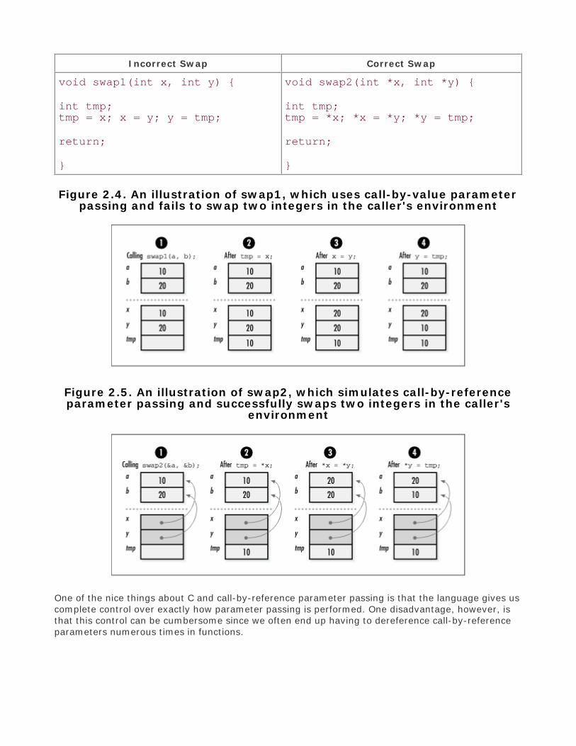
To understand how this works, first consider swap1, which illustrates an incorrect implementation ofa function to swap two integers using call-by-value parameter passing without pointers. Figure 2.4illustrates why this does not work. The function swap2 corrects the problem by using pointers tosimulate call-by-reference parameter passing. Figure 2.5 illustrates how using pointers makesswapping proceed correctly.
Figure 2.4. An illustration of swap1, which uses call-by-value parameterpassing and fails to swap two integers in the caller's environment
Incorrect Swap Correct Swap
void swap1(int x, int y) {
int tmp;tmp = x; x = y; y = tmp;
return;
}
void swap2(int *x, int *y) {
int tmp;tmp = *x; *x = *y; *y = tmp;
return;
}
Figure 2.4. An illustration of swap1, which uses call-by-value parameterpassing and fails to swap two integers in the caller's environment
Figure 2.5. An illustration of swap2, which simulates call-by-referenceparameter passing and successfully swaps two integers in the caller's
environment
One of the nice things about C and call-by-reference parameter passing is that the language gives uscomplete control over exactly how parameter passing is performed. One disadvantage, however, isthat this control can be cumbersome since we often end up having to dereference call-by-referenceparameters numerous times in functions.
Another use of pointers in function calls occurs when we pass arrays to functions. Recalling that Ctreats all array names transparently as unmodifiable pointers, passing an array of objects of type Tin a function is equivalent to passing a pointer to an object of type T. Thus, we can use the twoapproaches interchangeably. For example, function f1 and function f2 are equivalent.
Array Reference Pointer Reference
int f1(int a[]) {
a[0] = 5;
return 0;
}
int f2(int *a) {
*a = 5;
return 0;
}
Usually the approach chosen depends on a convention or on wanting to convey something about howthe parameter is used in the function. When using an array parameter, bounds information is oftenomitted since it is not required by the compiler. However, including bounds information can be auseful way to document a limit the function imposes on a parameter internally. Bounds informationplays a more critical role with array parameters that are multidimensional.
When defining a function that accepts a multidimensional array, all but the first dimension must bespecified so that pointer arithmetic can be performed when elements are accessed, as shown in thefollowing code:
int g(int a[][2]) {
a[2][0] = 5;
return 0;
}
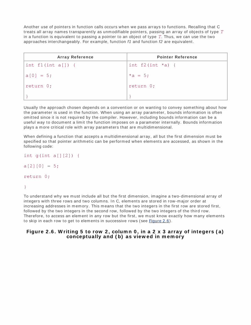
To understand why we must include all but the first dimension, imagine a two-dimensional array ofintegers with three rows and two columns. In C, elements are stored in row-major order atincreasing addresses in memory. This means that the two integers in the first row are stored first,followed by the two integers in the second row, followed by the two integers of the third row.Therefore, to access an element in any row but the first, we must know exactly how many elementsto skip in each row to get to elements in successive rows (see Figure 2.6).
Figure 2.6. Writing 5 to row 2, column 0, in a 2 x 3 array of integers (a)conceptually and (b) as viewed in memory

2.4.2 Pointers to Pointers as Parameters
One situation in which pointers are used as parameters to functions a great deal in this book is whena function must modify a pointer passed into it. To do this, the function is passed a pointer to thepointer to be modified. Consider the operation list_rem_next, which Chapter 5 defines for removingan element from a linked list. Upon return, data points to the data removed from the list:
int list_rem_next(List *list, ListElmt *element, void **data);
Since the operation must modify the pointer data to make it point to the data removed, we mustpass the address of the pointer data in order to simulate call-by-reference parameter passing (seeFigure 2.7). Thus, the operation takes a pointer to a pointer as its third parameter. This is typical ofhow data is removed from most of the data structures presented in this book.
Figure 2.7. Using a function to modify a pointer to point to an integerremoved from a linked list
Top
Mastering Algorithms with CBy Kyle Loudon
Slots : 1
Table of Contents
Chapter 2. Pointer Manipulation
Content
2.5 Generic Pointers and Casts
Recall that pointer variables in C have types just like other variables. The main reason for this is sothat when we dereference a pointer, the compiler knows the type of data being pointed to and canaccess the data accordingly. However, sometimes we are not concerned about the type of data apointer references. In these cases we use generic pointers, which bypass C's type system.
2.5.1 Generic Pointers
Normally C allows assignments only between pointers of the same type. For example, given acharacter pointer sptr (a string) and an integer pointer iptr, we are not permitted to assign sptrto iptr or iptr to sptr. However, generic pointers can be set to pointers of any type, and viceversa. Thus, given a generic pointer gptr, we are permitted to assign sptr to gptr or gptr tosptr. To make a pointer generic in C, we declare it as a void pointer .
There are many situations in which void pointers are useful. For example, consider the standard Clibrary function memcpy, which copies a block of data from one location in memory to another.Because memcpy may be used to copy data of any type, it makes sense that its pointer parametersare void pointers. Void pointers can be used to make other types of functions more generic as well.For example, we might have implemented the swap2 function presented earlier so that it swappeddata of any type, as shown in the following code:
#include <stdlib.h>#include <string.h>
int swap2(void *x, void *y, int size) {
void *tmp;
if ((tmp = malloc(size)) == NULL) return -1;
memcpy(tmp, x, size); memcpy(x, y, size); memcpy(y, tmp, size);free(tmp);

return 0;
}
Void pointers are particularly useful when implementing data structures because they allow us tostore and retrieve data of any type. Consider again the ListElmt structure presented earlier forlinked lists. Recall that this structure contains two members, data and next. Since data isdeclared as a void pointer, it can point to data of any type. Thus, we can use ListElmt structuresto build any type of list.
In Chapter 5, one of the operations defined for linked lists is list_ins_next, which accepts a voidpointer to the data to be inserted:
int list_ins_next(List *list, ListElmt *element, void *data);
To insert an integer referenced by iptr into a list of integers, list, after an element referenced byelement, we use the following call. C permits us to pass the integer pointer iptr for theparameter data because data is a void pointer.
retval = list_ins_next(&list, element, iptr);
Of course, when removing data from the list, it is important to use the correct type of pointer toretrieve the data removed. Doing so ensures that the data will be interpreted correctly if we try to dosomething with it. As discussed earlier, the operation for removing an element from a linked list islist_rem_next (see Chapter 5), which takes a pointer to a void pointer as its third parameter:
int list_rem_next(List *list, ListElmt *element, void **data);
To remove an integer from list after an element referenced by element, we use the followingcall. Upon return, iptr points to the data removed. We pass the address of the pointer iptr sincethe operation modifies the pointer itself to make it point to the data removed.
retval = list_rem_next(&list, element, (void **)&iptr);
This call also includes a cast to make iptr temporarily appear as a pointer to a void pointer, sincethis is what list_rem_next requires. As we will see in the next section, casting is a mechanism in Cthat lets us temporarily treat a variable of one type as a variable of another type. A cast is necessaryhere because, although a void pointer is compatible with any other type of pointer in C, a pointer to avoid pointer is not.
2.5.2 Casts
To cast a variable t of some type T to another type S, we precede t with S in parentheses. Forexample, to assign an integer pointer iptr to a floating-point pointer fptr, we cast iptr to afloating-point pointer and then carry out the assignment, as shown:
fptr = (float *)iptr;
(Although casting an integer pointer to a floating-point pointer is a dangerous practice in general, it ispresented here as an illustration.) After the assignment, iptr and fptr both contain the sameaddress. However, the interpretation of the data at this address depends on which pointer we use toaccess it.

Casts are especially important with generic pointers because generic pointers cannot be dereferencedwithout casting them to some other type. This is because generic pointers give the compiler noinformation about what is being pointed to; thus, it is not clear how many bytes should be accessed,nor how the bytes should be interpreted. Casts are also a nice form of self-documentation whengeneric pointers are assigned to pointers of other types. Although the cast is not necessary in thiscase, it does improve a program's readability.
When casting pointers, one issue we need to be particularly sensitive to is the way data is aligned inmemory. Specifically, we need to be aware that applying casts to pointers can undermine thealignment a computer expects. Often computers have alignment requirements so that certainhardware optimizations can make accessing memory more efficient. For example, a system mayinsist that all integers be aligned on word boundaries. Thus, given a void pointer that is not wordaligned, if we cast the void pointer to an integer pointer and dereference it, we can expect anexception to occur at runtime.
Top

Mastering Algorithms with CBy Kyle Loudon
Slots : 1
Table of Contents
Chapter 2. Pointer Manipulation
Content
2.6 Function Pointers
Function pointers are pointers that, instead of pointing to data, point to executable code or to blocksof information needed to invoke executable code. They are used to store and manage functions as ifthey were pieces of data. Function pointers have a type that is described in terms of a return valueand parameters that the function accepts. Declarations for function pointers look much likedeclarations for functions, except that an asterisk ( * ) appears before the function name, and theasterisk and name are surrounded by parentheses for reasons of associativity. For example, in thefollowing code, match is declared as a pointer to a function that accepts two void pointers andreturns an integer:
int (*match)(void *key1, void *key2);
This declaration means that we can set match to point to any function that accepts two voidpointers and returns an integer. For example, suppose match_int is a function that accepts two voidpointers to integers and returns 1 if the integers match, or otherwise. Assuming the previousdeclaration, we could set match to point to this function by executing the following statement:
match = match_int;
To execute a function referenced by a function pointer, we simply use the function pointer whereverwe would normally use the function itself. For example, to invoke the function referenced by matchearlier, we execute the following statement, assuming x, y, and retval have been declared asintegers:
retval = match(&x, &y);
One important use of function pointers in this book is to encapsulate functions into data structures.For example, in the implementation of chained hash tables (see Chapter 8), the data structure has amatch member similar to the function pointer just described. This pointer is used to invoke afunction whenever we need to determine whether an element we are searching for matches anelement in the table. We assign a function to this pointer when the table is initialized. The function weassign has the same prototype as match but internally compares two elements of the appropriatetype, depending on the type of data in the table for which the table has been defined. Using a pointerto store a function as part of a data structure is nice because it is yet another way to keep animplementation generic.

Top

Mastering Algorithms with CBy Kyle Loudon
Slots : 1
Table of Contents
Chapter 2. Pointer Manipulation
Content
2.7 Questions and Answers
Q: One of the difficulties with pointers is that often when we misuse them, our errors are not caughtby the compiler at compile time; they occur at runtime. Which of the following result in compile-timeerrors? Which of the following result in runtime errors? Why?
a)
char *sptr = "abc",*tptr;*tptr = sptr;
b)
char *sptr = "abc",*tptr;tptr = sptr;
c)
char *sptr = "abc",*tptr;*tptr = *sptr;
d)
int *iptr = (int *)10;*iptr = 11;
e)
int *iptr = 10;*iptr = 11;
f )
int *iptr = (int *)10;iptr = NULL;
A: a) A compile-time error occurs because when we dereference tptr, we get a character, whereassptr is a pointer to a character. Thus, the code is trying to assign a character pointer to acharacter, which is a type conflict. b) No error occurs because both tptr and sptr are characterpointers. c) A runtime error is likely to occur because no storage has been allocated for tptr. Whenwe dereference tptr, we cannot be sure where it points. d) A runtime error is likely to occurbecause assigning an integer pointer a fixed address is dangerous. When dereferencing iptr, we tryto write 11 at address 10, which is probably invalid. e) A compile-time error or warning occursbecause the code is trying to initialize an integer pointer to an integer, which is a type conflict. f ) Noerror occurs because although the code first performs the dangerous step of initializing iptr to afixed address, it is then immediately reset to NULL, which is valid.
Q: Recall that calculations with pointers are performed using pointer arithmetic. If p contains theaddress 0x10000000, what address does the following expression access? How many bytes areaccessed at this address?
*(p + 5)

A: The answer to this question depends on the type of p. Recall that when we add an integer i to apointer p, the result is not the address stored in p plus i bytes, but the address in p, plus i times thenumber of bytes in the datatype p references. Since the question does not state p 's type, it is notpossible to determine the address accessed as a result of the expression. The type of p is alsorequired to determine how many bytes p accesses. Therefore, it is also impossible to determine thenumber of bytes accessed.
Q: The operation list_rem_next removes an element from a linked list (see Chapter 5). If iptr is aninteger pointer we would like set to an integer removed from a list, how might we call list_rem_nextas an alternative to the approach presented in the chapter? A prototype for the function is shownhere, where list is the list, element references the element preceding the one to remove, andupon return, data references the data removed.
int list_rem_next(List *list, ListElmt *element, void **data);
A: An alternative way to call list_rem_next is shown here. In this approach, iptr is cast to a voidpointer instead of a pointer to a void pointer. This method is acceptable because void pointers arecompatible with all others. However, our original approach is clearer because it is consistent with theprototype of list_rem_next.
retval = list_rem_next(&list, element, (void *)&iptr);
Top

Mastering Algorithms with CBy Kyle Loudon
Slots : 1
Table of Contents
Chapter 2. Pointer Manipulation
Content
2.8 Related Topics
C++
An object-oriented language that enforces many practices of good software engineering. Asone example, it supports constructors and destructors for datatypes. These mechanismsprovide a compact way of managing memory within instances of the type, thus avoiding manyof the problems associated with memory leaks and pointers in C.
Heap-based allocation
The type of memory allocation provided by the C functions malloc and realloc. Heap-basedallocation is often called dynamic storage allocation. This allows a program to request morememory as it needs it rather than allocating a fixed amount at compile time.
Top
Mastering Algorithms with CBy Kyle Loudon
Slots : 1
Table of Contents
Part I: Preliminaries
Content
Chapter 3. RecursionRecursion is a powerful principle that allows something to be defined in terms of smaller instances ofitself. Perhaps there is no better way to appreciate the significance of recursion than to look at themysterious ways nature uses it. Think of the fragile leaf of a fern, in which each individual sprig fromthe leaf's stem is just a smaller copy of the overall leaf; or the repeating patterns in a reflection, inwhich two shiny objects reflect each other. Examples like these convince us that even though natureis a great force, in many ways it has a paradoxical simplicity that is truly elegant. The same can besaid for recursive algorithms; in many ways, recursive algorithms are simple and elegant, yet theycan be extremely powerful.
In computing, recursion is supported via recursive functions. A recursive function is a function thatcalls itself. Each successive call works on a more refined set of inputs, bringing us closer and closer tothe solution of a problem. Most developers are comfortable with the idea of dividing a larger probleminto several smaller ones and writing separate functions to solve them. However, many developersare less comfortable with the idea of solving a larger problem with a single function that calls itself.Admittedly, looking at a problem in this way can take some getting used to. This chapter exploreshow recursion works and shows how to define some problems in a recursive manner. Some examplesof recursive approaches in this book are found in tree traversals (see Chapter 9), breadth-first anddepth-first searches with graphs (see Chapter 11), and sorting (see Chapter 12 ).
This chapter covers:
Basic recursion
A powerful principle that allows a problem to be defined in terms of smaller and smallerinstances of itself. In computing, we solve problems defined recursively by using recursivefunctions, which are functions that call themselves.
Tail recursion
A form of recursion for which compilers are able to generate optimized code. Most moderncompilers recognize tail recursion. Therefore, we should make use of it whenever we can.
Top
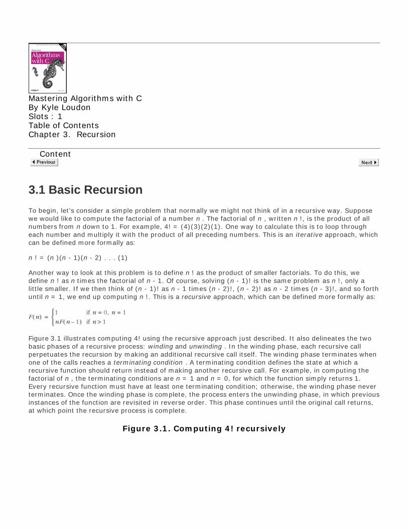
Mastering Algorithms with CBy Kyle LoudonSlots : 1Table of ContentsChapter 3. Recursion
Content
3.1 Basic Recursion
To begin, let's consider a simple problem that normally we might not think of in a recursive way. Supposewe would like to compute the factorial of a number n . The factorial of n , written n !, is the product of allnumbers from n down to 1. For example, 4! = (4)(3)(2)(1). One way to calculate this is to loop througheach number and multiply it with the product of all preceding numbers. This is an iterative approach, whichcan be defined more formally as:
n ! = (n )(n - 1)(n - 2) . . . (1)
Another way to look at this problem is to define n ! as the product of smaller factorials. To do this, wedefine n ! as n times the factorial of n - 1. Of course, solving (n - 1)! is the same problem as n !, only alittle smaller. If we then think of (n - 1)! as n - 1 times (n - 2)!, (n - 2)! as n - 2 times (n - 3)!, and so forthuntil n = 1, we end up computing n !. This is a recursive approach, which can be defined more formally as:
Figure 3.1 illustrates computing 4! using the recursive approach just described. It also delineates the twobasic phases of a recursive process: winding and unwinding . In the winding phase, each recursive callperpetuates the recursion by making an additional recursive call itself. The winding phase terminates whenone of the calls reaches a terminating condition . A terminating condition defines the state at which arecursive function should return instead of making another recursive call. For example, in computing thefactorial of n , the terminating conditions are n = 1 and n = 0, for which the function simply returns 1.Every recursive function must have at least one terminating condition; otherwise, the winding phase neverterminates. Once the winding phase is complete, the process enters the unwinding phase, in which previousinstances of the function are revisited in reverse order. This phase continues until the original call returns,at which point the recursive process is complete.
Figure 3.1. Computing 4! recursively

Example 3.1 presents a C function, fact , that accepts a number n and computes its factorial recursively.
The function works as follows. If n is less than 0, the function returns 0, indicating an error. If n is or 1,
the function returns 1 because 0! and 1! are both defined as 1. These are the terminating conditions.
Otherwise, the function returns the result of n times the factorial of n - 1. The factorial of n - 1 is
computed recursively by calling fact again, and so forth. Notice the similarities between this implementationand the recursive definition shown earlier.
Example 3.1. Implementation of a Function for Computing FactorialsRecursively
/****************************************************************************** ** -------------------------------- fact.c -------------------------------- ** ******************************************************************************/
#include "fact.h"
/****************************************************************************** ** --------------------------------- fact --------------------------------- ** ******************************************************************************/
int fact(int n) {
/****************************************************************************** ** Compute a factorial recursively. ** ******************************************************************************/
if (n < 0) return 0;else if (n == 0) return 1;

else if (n == 1) return 1;else return n * fact(n - 1);
}
To understand how recursion really works, it helps to look at the way functions are executed in C. For this,we need to understand a little about the organization of a C program in memory . Fundamentally, a Cprogram consists of four areas as it executes: a code area, a static data area, a heap, and a stack (seeFigure 3.2 a). The code area contains the machine instructions that are executed as the program runs. Thestatic data area contains data that persists throughout the life of the program, such as global variables andstatic local variables. The heap contains dynamically allocated storage, such as memory allocated by malloc. The stack contains information about function calls. By convention, the heap grows upward from one endof a program's memory, while the stack grows downward from the other (but this may vary in practice).Note that the term heap as it is used in this context has nothing to do with the heap data structurepresented in Chapter 10 .
When a function is called in a C program, a block of storage is allocated on the stack to keep track ofinformation associated with the call. Each call is referred to as an activation . The block of storage placedon the stack is called an activation record or, alternatively, a stack frame . An activation record consists offive regions: incoming parameters, space for a return value, temporary storage used in evaluatingexpressions, saved state information for when the activation terminates, and outgoing parameters (seeFigure 3.2 b). Incoming parameters are the parameters passed into the activation. Outgoing parametersare the parameters passed to functions called within the activation. The outgoing parameters of oneactivation record become the incoming parameters of the next one placed on the stack. The activationrecord for a function call remains on the stack until the call terminates.
Returning to Example 3.1 , consider what happens on the stack as one computes 4!. The initial call to factresults in one activation record being placed on the stack with an incoming parameter of n = 4 (see Figure3.3 , step 1). Since this activation does not meet any of the terminating conditions of the function, fact isrecursively called with n set to 3. This places another activation of fact on the stack, but with an incomingparameter of n = 3 (see Figure 3.3 , step 2). Here, n = 3 is also an outgoing parameter of the firstactivation since the first activation invoked the second. The process continues this way until n is 1, at whichpoint a terminating condition is encountered and fact returns 1 (see Figure 3.3 , step 4).
Figure 3.2. The organization in memory of (a) a C program and (b) anactivation record
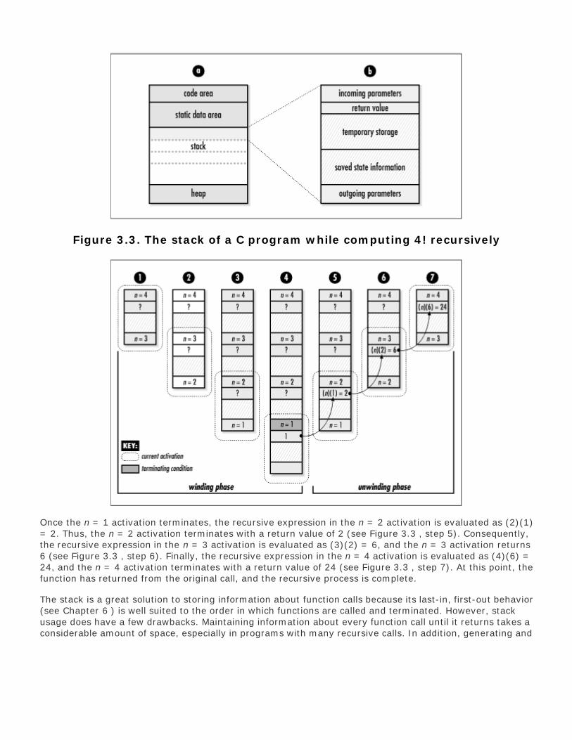
Figure 3.3. The stack of a C program while computing 4! recursively
Once the n = 1 activation terminates, the recursive expression in the n = 2 activation is evaluated as (2)(1)= 2. Thus, the n = 2 activation terminates with a return value of 2 (see Figure 3.3 , step 5). Consequently,the recursive expression in the n = 3 activation is evaluated as (3)(2) = 6, and the n = 3 activation returns6 (see Figure 3.3 , step 6). Finally, the recursive expression in the n = 4 activation is evaluated as (4)(6) =24, and the n = 4 activation terminates with a return value of 24 (see Figure 3.3 , step 7). At this point, thefunction has returned from the original call, and the recursive process is complete.
The stack is a great solution to storing information about function calls because its last-in, first-out behavior(see Chapter 6 ) is well suited to the order in which functions are called and terminated. However, stackusage does have a few drawbacks. Maintaining information about every function call until it returns takes aconsiderable amount of space, especially in programs with many recursive calls. In addition, generating and

destroying activation records takes time because there is a significant amount of information that must besaved and restored. Thus, if the overhead associated with these concerns becomes too great, we may needto consider an iterative approach. Fortunately, we can use a special type of recursion, called tail recursion ,to avoid these concerns in some cases .
Top

Mastering Algorithms with CBy Kyle LoudonSlots : 1Table of ContentsChapter 3. Recursion
Content
3.2 Tail Recursion
A recursive function is said to be tail recursive if all recursive calls within it are tail recursive. A recursivecall is tail recursive when it is the last statement that will be executed within the body of a function and itsreturn value is not a part of an expression. Tail-recursive functions are characterized as having nothing todo during the unwinding phase. This characteristic is important because most modern compilersautomatically generate code to take advantage of it.
When a compiler detects a call that is tail recursive, it overwrites the current activation record instead ofpushing a new one onto the stack. The compiler can do this because the recursive call is the last statementto be executed in the current activation; thus, there is nothing left to do in the activation when the callreturns. Consequently, there is no reason to keep the current activation around. By replacing the currentactivation record instead of stacking another one on top of it, stack usage is greatly reduced, which leads tobetter performance in practice. Thus, we should make recursive functions tail recursive whenever we can.
To understand how tail recursion works, let's revisit computing a factorial recursively. First, it is helpful tounderstand the reason the previous definition was not tail recursive. Recall that the original definitioncomputed n ! by multiplying n times (n - 1)! in each activation, repeating this for n = n - 1 until n = 1. Thisdefinition was not tail recursive because the return value of each activation depended on multiplying ntimes the return value of subsequent activations. Therefore, the activation record for each call had toremain on the stack until the return values of subsequent calls were determined. Now consider a tail-recursive definition for computing n !, which can be defined formally as:
This definition is similar to the one presented earlier, except that it uses a second parameter, a (initially setto 1), which maintains the value of the factorial computed thus far in the recursive process. This preventsus from having to multiply the return value of each activation by n . Instead, in each recursive call, we let a= na and n = n - 1. We continue this until n = 1, which is the terminating condition, at which point wesimply return a . Figure 3.4 illustrates the process of computing 4! using this approach. Notice how there isno work that needs to be performed during the unwinding phase, a signature of all tail-recursive functions.
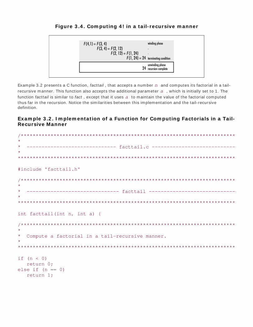
Figure 3.4. Computing 4! in a tail-recursive manner
Example 3.2 presents a C function, facttail , that accepts a number n and computes its factorial in a tail-
recursive manner. This function also accepts the additional parameter a , which is initially set to 1. The
function facttail is similar to fact , except that it uses a to maintain the value of the factorial computed
thus far in the recursion. Notice the similarities between this implementation and the tail-recursivedefinition.
Example 3.2. Implementation of a Function for Computing Factorials in a Tail-Recursive Manner
/****************************************************************************** ** ------------------------------ facttail.c ------------------------------ ** ******************************************************************************/
#include "facttail.h"
/****************************************************************************** ** ------------------------------- facttail ------------------------------- ** ******************************************************************************/
int facttail(int n, int a) {
/****************************************************************************** ** Compute a factorial in a tail-recursive manner. ** ******************************************************************************/
if (n < 0) return 0;else if (n == 0) return 1;

else if (n == 1) return a;else return facttail(n - 1, n * a);
}
The function in Example 3.2 is tail recursive because the single recursive call to facttail is the last statementexecuted before returning from the call. It just happens that this is the last statement of facttail as well,but this does not have to be the case. In other words, there could have been other statements after therecursive call, provided they were executed only when the recursive call was not. Figure 3.5 illustrates thelimited activity on the stack while computing 4! using this tail-recursive function. Contrast this with theactivity on the stack in Figure 3.3 .
Figure 3.5. The stack of a C program while computing 4! in a tail-recursivemanner
Top

Mastering Algorithms with CBy Kyle Loudon
Slots : 1
Table of Contents
Chapter 3. Recursion
Content
3.3 Questions and Answers
Q: The following recursive definition has an error. What is it, and how can we fix it? For a positiveinteger n, the definition, in its proper form, is common in formally computing the running time ofdivide-and-conquer algorithms, such as merge sort (see Chapter 12). Merge sort divides a set of datain half, then divides the halves in half, and continues this way until each division contains a singleelement. Then, during the unwinding phase, the divisions are merged to produce a final sorted set.
A: The problem with this definition is that it never reaches the terminating condition, n = 0, for anyinitial value of n greater than 0. To fix the problem, it needs an obtainable terminating condition. Thecondition n = 1 works well, which means we should also change the second condition in the function.A recursive definition with an acceptable terminating condition is presented here:
This happens to be the correct definition for the running time of merge sort. Such a function is calleda recurrence. In more formal analysis, recurrences are used frequently to describe the running timesof recursive algorithms.
Q: Describe a recursive approach for computing the prime factors of a number. Determine whetherthe approach is tail recursive, and describe why or why not.
A: Recursion is a natural way to find the prime factors of a number because factoring is really justthe same problem over and over again, only a little smaller, as we determine each factor. A recursiveapproach to this problem can be defined as shown:
This definition says that to determine the prime factors of a number n recursively, determine itssmallest prime factor i, record this in a set of factors P, and repeat the process for n = n /i. Continue

this way until n is found to be prime itself, which is the terminating condition. This definition is tailrecursive because there is nothing that needs to be done during the unwinding phase, as Figure 3.6confirms.
Figure 3.6. Computing the prime factors of 2409 in a tail-recursivemanner
Q: Considering how the stack is used in executing recursive functions, what happens when thewinding phase of a recursive process never terminates, perhaps as a result of a malformedterminating condition, as in the first question?
A: If the terminating condition of a recursive function is never reached, eventually the stack growspast an acceptable size and the program aborts from a stack overflow. A special pointer, called theframe pointer, keeps track of the top of the stack as a program executes. It is also used to determinewhen the stack has grown too large. An interrupt is raised to signal the error.
Q: Recursive functions frequently offer simple yet concise ways to describe useful computations.Describe the computation that the following recursive definition describes:
A: This recursive definition calculates a series like the following one, called the harmonic series. Forpositive integers n, the function calculates the n th harmonic number. (The calculation proceeds inreverse order from what is shown, but the following form is more recognizable.)
Q: Is the function in the previous question tail recursive? If so, describe why. If not, describe why notand present a tail-recursive version.
A: The function defined in the previous question is not tail recursive because the return value of therecursive call is used in an expression. This expression becomes the return value of the current call.Therefore, each activation must remain on the stack until it gets the return value of subsequentactivations. To make this function tail recursive, we can use an approach like the one presentedearlier in the chapter for computing a factorial in a tail-recursive manner. We use an additionalparameter a to keep a tally of the total value of the series computed thus far in the recursion.Formally, a tail-recursive version of the function in the previous question is as follows:

Top

Mastering Algorithms with CBy Kyle Loudon
Slots : 1
Table of Contents
Chapter 3. Recursion
Content
3.4 Related Topics
Compiler design
The basics behind the code translators that ultimately dictate how efficiently programs will run,at least at the instruction level. Whereas generally in algorithm design we focus on complexityas a measure of performance (see Chapter 4), understanding the issues compilers deal with intranslating code can help us tune performance in practice. Understanding tail recursion is agood example.
Tail recursion elimination
A process in which the final tail-recursive call in a function is replaced with an iterative controlstructure. This does not change the outcome of the function, but helps avoid the overhead ofan extra function call. Tail recursion elimination is a fundamental principle studied in compilerdesign.
Recursion trees
Illustrations that help us visualize calling sequences with recursive functions. Recursion treesvary in their formality. Figures Figure 3.1 and Figure 3.4 for recursively computing a factorialand Figure 3.6 for determining the prime factors of a number are recursion trees. Recursiontrees are most often used with functions containing two or more recursive calls within eachactivation.
Top

Mastering Algorithms with CBy Kyle Loudon
Slots : 1
Table of Contents
Part I: Preliminaries
Content
Chapter 4. Analysis of AlgorithmsWhether we are designing an algorithm or applying one that is widely accepted, it is important tounderstand how the algorithm will perform. There are a number of ways we can look at analgorithm's performance, but usually the aspect of most interest is how fast the algorithm will run. Insome cases, if an algorithm uses significant storage, we may be interested in its space requirementas well. Whatever the case, determining how an algorithm performs requires a formal anddeterministic method.
There are many reasons to understand the performance of an algorithm. For example, we often havea choice of several algorithms when solving problems. Understanding how each performs helps usdifferentiate between them. Understanding the burden an algorithm places on an application alsohelps us plan how to use the algorithm more effectively. For instance, garbage collection algorithms,algorithms that collect dynamically allocated storage to return to the heap (see Chapter 3), requireconsiderable time to run. Knowing this, we can be careful to run them only at opportune moments,just as LISP and Java do, for example.
This chapter covers:
Worst-case analysis
The metric by which most algorithms are compared. Other cases we might consider are theaverage case and best case. However, worst-case analysis usually offers several advantages.
O-notation
The most common notation used to formally express an algorithm's performance. O -notationis used to express the upper bound of a function within a constant factor.
Computational complexity
The growth rate of the resources (usually time) an algorithm requires with respect to the sizeof the data it processes. O -notation is a formal expression of an algorithm's complexity.
Top

Mastering Algorithms with CBy Kyle Loudon
Slots : 1
Table of Contents
Chapter 4. Analysis of Algorithms
Content
4.1 Worst-Case Analysis
Most algorithms do not perform the same in all cases; normally an algorithm's performance varieswith the data passed to it. Typically, three cases are recognized: the best case, worst case, andaverage case. For any algorithm, understanding what constitutes each of these cases is an importantpart of analysis because performance can vary significantly between them. Consider even a simplealgorithm such as linear search. Linear search is a natural but inefficient search technique in whichwe look for an element simply by traversing a set from one end to the other. In the best case, theelement we are looking for is the first element we inspect, so we end up traversing only a singleelement. In the worst case, however, the desired element is the last one we inspect, in which casewe end up traversing all of the elements. On average, we can expect to find the element somewherein the middle.
4.1.1 Reasons for Worst-Case Analysis
A basic understanding of how an algorithm performs in all cases is important, but usually we aremost interested in how an algorithm performs in the worst case. There are four reasons whyalgorithms are generally analyzed by their worst case:
Many algorithms perform to their worst case a large part of the time. For example, the worstcase in searching occurs when we do not find what we are looking for at all. Imagine howfrequently this takes place in some database applications.
The best case is not very informative because many algorithms perform exactly the same in thebest case. For example, nearly all searching algorithms can locate an element in one inspectionat best, so analyzing this case does not tell us much.
Determining average-case performance is not always easy. Often it is difficult to determineexactly what the "average case" even is. Since we can seldom guarantee precisely how analgorithm will be exercised, usually we cannot obtain an average-case measurement that islikely to be accurate.
The worst case gives us an upper bound on performance. Analyzing an algorithm's worst caseguarantees that it will never perform worse than what we determine. Therefore, we know thatthe other cases must perform at least as well.
Although worst-case analysis is the metric for many algorithms, it is worth noting that there areexceptions. Sometimes special circumstances let us base performance on the average case. Forexample, randomized algorithms such as quicksort (see Chapter 12 ) use principles of probability tovirtually guarantee average-case performance.
Top

Mastering Algorithms with CBy Kyle Loudon
Slots : 1
Table of Contents
Chapter 4. Analysis of Algorithms
Content
4.2 O-Notation
O -notation is the most common notation used to express an algorithm's performance in a formalmanner. Formally, O -notation expresses the upper bound of a function within a constant factor.Specifically, if g (n) is an upper bound of f (n), then for some constant c it is possible to find a value
of n, call it n0, for which any value of n n0 will result in f (n) cg (n).
Normally we express an algorithm's performance as a function of the size of the data it processes.That is, for some data of size n, we describe its performance with some function f (n). However, whilein many cases we can determine f exactly, usually it is not necessary to be this precise. Primarily weare interested only in the growth rate of f, which describes how quickly the algorithm's performancewill degrade as the size of the data it processes becomes arbitrarily large. An algorithm's growthrate, or order of growth, is significant because ultimately it describes how efficient the algorithm is forarbitrary inputs. O -notation reflects an algorithm's order of growth.
4.2.1 Simple Rules for O-Notation
When we look at some function f (n) in terms of its growth rate, a few things become apparent. First,we can ignore constant terms because as the value of n becomes larger and larger, eventuallyconstant terms will become insignificant. For example, if T (n) = n + 50 describes the running time ofan algorithm, and n, the size of the data it processes, is only 1024, the constant term in thisexpression already constitutes less than 5% of the running time. Second, we can ignore constantmultipliers of terms because they too will become insignificant as the value of n increases. Forexample, if T1(n) = n2 and T2(n) = 10n describe the running times of two algorithms for solving thesame problem, n only has to be greater than 10 for T1 to become greater than T2. Finally, we needonly consider the highest-order term because, again, as n increases, higher-order terms quicklyoutweigh the lower-order ones. For example, if T (n) = n2 + n describes the running time of analgorithm, and n is 1024, the lesser-order term of this expression constitutes less than 0.1% of therunning time. These ideas are formalized in the following simple rules for expressing functions in O -notation.
Constant terms are expressed as O (1). When analyzing the running time of an algorithm, applythis rule when you have a task that you know will execute in a certain amount of timeregardless of the size of the data it processes. Formally stated, for some constant c:

O(c) = O(1)
Multiplicative constants are omitted. When analyzing the running time of an algorithm, applythis rule when you have a number of tasks that all execute in the same amount of time. Forexample, if three tasks each run in time T (n) = n, the result is O (3n), which simplifies to O (n).Formally stated, for some constant c:
O(cT) = cO(T) = O(T)
Addition is performed by taking the maximum. When analyzing the running time of analgorithm, apply this rule when one task is executed after another. For example, if T1(n) = nand T2(n) = n2 describe two tasks executed sequentially, the result is O (n) + O (n2), whichsimplifies to O (n2). Formally stated:
O(T1)+O(T1+T2) = max (O(T1), O(T2))
Multiplication is not changed but often is rewritten more compactly. When analyzing the runningtime of an algorithm, apply this rule when one task causes another to be executed somenumber of times for each iteration of itself. For example, in a nested loop whose outer iterationsare described by T1 and whose inner iterations by T2, if T1(n) = n and T2(n) = n, the result is O(n)O (n), or O (n2). Formally stated:
O(T1)O(T2) = O(T1 T2)
4.2.2 O-Notation Example and Why It Works
The next section discusses how these rules help us in predicting an algorithm's performance. Fornow, let's look at a specific example demonstrating why they work so well in describing a function'sgrowth rate. Suppose we have an algorithm whose running time is described by the function T (n) =3n2 + 10n + 10. Using the rules of O -notation, this function can be simplified to:
O(T(n)) = O(3n2 + 10n + 10) = O(3n2) = O(n2)
This indicates that the term containing n2 will be the one that accounts for most of the running timeas n grows arbitrarily large. We can verify this quantitatively by computing the percentage of theoverall running time that each term accounts for as n increases. For example, when n = 10, we havethe following:
Running time for 3n2: 3(10)2/(3(10)2 + 10(10) + 10) = 73.2%Running time for 10n: 10(10)/(3(10)2 + 10(10) + 10) = 24.4%Running time for 10: 10/(3(10)2 + 10(10) + 10) = 2.4%
Already we see that the n2 term accounts for the majority of the overall running time. Now considerwhen n = 100:
Running time for 3n2: 3(100)2/(3(100)2 + 10(100) + 10) = 96.7% (Higher)Running time for 10n: 10(100)/(3(100)2 + 10(100) + 10) = 3.2% (Lower)Running time for 10: 10/(3(100)2 + 10(100) + 10) < 0.1% (Lower)
Here we see that this term accounts for almost all of the running time, while the significance of theother terms diminishes further. Imagine how much of the running time this term would account for ifn were 106!

Top

Mastering Algorithms with CBy Kyle Loudon
Slots : 1
Table of Contents
Chapter 4. Analysis of Algorithms
Content
4.3 Computational Complexity
When speaking of the performance of an algorithm, usually the aspect of interest is its complexity,which is the growth rate of the resources (usually time) it requires with respect to the size of thedata it processes. O -notation describes an algorithm's complexity. Using O -notation, we canfrequently describe the worst-case complexity of an algorithm simply by inspecting its overallstructure. Other times, it is helpful to employ techniques involving recurrences and summationformulas (see the related topics at the end of the chapter), and statistics.
To understand complexity, let's look at one way to surmise the resources an algorithm will require. Itshould seem reasonable that if we look at an algorithm as a series of k statements, each with somecost (usually time) to execute, ci , we can determine the algorithm's total cost by summing the costsof all statements from c1 to ck in whatever order each is executed. Normally statements areexecuted in a more complicated manner than simply in sequence, so this has to be taken intoaccount when totaling the costs. For example, if some subset of the statements is executed in a loop,the costs of the subset must be multiplied by the number of iterations. Consider an algorithmconsisting of k = 6 statements. If statements 3, 4, and 5 are executed in a loop from 1 to n and theother statements are executed sequentially, the overall cost of the algorithm is:
T(n) = c1 + c2 + n(c3 + c4 + c5) + c6
Using the rules of O -notation, this algorithm's complexity is O (n) because the constants are notsignificant. Analyzing an algorithm in terms of these constant costs is very thorough. However,recalling what we have seen about growth rates, remember that we do not need to be so precise.When inspecting the overall structure of an algorithm, only two steps need to be performed: we mustdetermine which parts of the algorithm depend on data whose size is not constant, and then derivefunctions that describe the performance of each part. All other parts of the algorithm execute with aconstant cost and can be ignored in figuring its overall complexity.
Assuming T (n) in the previous example represents an algorithm's running time, it is important torealize that O (n), its complexity, says little about the actual time the algorithm will take to run. Inother words, just because an algorithm has a low growth rate does not necessarily mean it willexecute in a small amount of time. In fact, complexities have no real units of measurement at all.They describe only how the resource being measured will be affected by a change in data size. Forexample, saying that T (n) is O (n) conveys only that the algorithm's running time variesproportionally to n, and that n is an upper bound for T (n) within a constant factor. Formally, we say
that T (n) cn, where c is a constant factor that accounts for various costs not associated with the

data, such as the type of computer on which the algorithm is running, the compiler used to generatethe machine code, and constants in the algorithm itself.
Many complexities occur frequently in computing, so it is worthwhile to become familiar with them.Table 4.1 lists some typical situations in which common complexities occur. Table 4.2 lists thesecommon complexities along with some calculations illustrating their growth rates. Figure 4.1 presentsthe data of Table 4.2 in a graphical form.
Table 4.1. Some Situations Wherein Common Complexities Occur
Complexity Example
O(1) Fetching the first element from a set of data
O(lg n) Splitting a set of data in half, then splitting the halves in half, etc.
O(n) Traversing a set of data
O(n lg n) Splitting a set of data in half repeatedly and traversing each half
O(n2) Traversing a set of data once for each member of another set of equal size
O(2n) Generating all possible subsets of a set of data
O(n!) Generating all possible permutations of a set of data
Table 4.2. The Growth Rates of the Complexities in Table 4.1
n = 1 n = 16 n = 256 n = 4K n = 64K n = 1M
O(1) 1.000E+00 1.000E+00 1.000E+00 1.000E+00 1.000E+00 1.000E+00
O (lg n) 0.000E+00 4.000E+00 8.000E+00 1.200E+01 1.600E+01 2.000E+01
O (n) 1.000E+00 1.600E+01 2.560E+02 4.096E+03 6.554E+04 1.049E+06
O (n lg n) 0.000E+00 6.400E+01 2.048E+03 4.915E+04 1.049E+06 2.097E+07
O (n2) 1.000E+00 2.560E+02 6.554E+04 1.678E+07 4.295E+09 1.100E+12
O (2n) 2.000E+00 6.554E+04 1.158E+77 — — —
O (n!) 1.000E+00 2.092E+13 — — — —
Figure 4.1. A graphical depiction of the growth rates in Tables Table 4.1and Table 4.2

Just as the complexity of an algorithm says little about its actual running time, it is important tounderstand that no measure of complexity is necessarily efficient or inefficient. Although complexityis an indication of the efficiency of an algorithm, whether a particular complexity is consideredefficient or inefficient depends on the problem. Generally, an efficient algorithm is one in which weknow we are doing the best we can do given certain criteria. Typically, an algorithm is said to beefficient if there are no algorithms with lower complexities to solve the same problem and thealgorithm does not contain excessive constants. Some problems are intractable, so there are no"efficient" solutions without settling for an approximation. This is true of a special class of problemscalled NP-complete problems (see the related topics at the end of the chapter).
Although an algorithm's complexity is an important starting point for determining how well it willperform, often there are other things to consider in practice. For example, when two algorithms areof the same complexity, it may be worthwhile to consider their less significant terms and factors. Ifthe data on which the algorithms' performances depend is small enough, even an algorithm ofgreater complexity with small constants may perform better in practice than one that has a lowerorder of complexity and larger constants. Other factors worth considering are how complicated analgorithm will be to develop and maintain, and how we can make the actual implementation of analgorithm more efficient. An efficient implementation does not always affect an algorithm'scomplexity, but it can reduce constant factors, which makes the algorithm run faster in practice.
Top

Mastering Algorithms with CBy Kyle LoudonSlots : 1Table of ContentsChapter 4. Analysis of Algorithms
Content
4.4 Analysis Example: Insertion Sort
This section presents an analysis of the worst-case running time of insertion sort , a simple sortingalgorithm that works by inserting elements into a sorted set by scanning the set to determine where eachnew element belongs. A complete description of insertion sort appears in Chapter 12 . The code for the sortis shown in Example 4.1 .
We begin by identifying which lines of code are affected by the size of the data to be sorted . These are the
statements that constitute the nested loop, whose outer part iterates from 1 to size - 1 and whose inner
part iterates from j - 1 to wherever the correct position for the element being inserted is found. All other
lines run in a constant amount of time, independent of the number of elements to be sorted. Typically, thegeneric variable n is used to refer to the parameter on which an algorithm's performance depends. Withthis in mind, the outer loop has a running time of T (n ) = n - 1, times some constant amount of time.Examining the inner loop and considering the worst case, we assume that we will have to go all the way tothe other end of the array before inserting each element into the sorted set. Therefore, the inner loopiterates once for the first element, twice for the second, and so forth until the outer loop terminates.Effectively, this becomes a summation from 1 to n - 1, which results in a running time of T (n ) = (n (n +1)/2) - n , times some constant amount of time. (This equation is from the well-known formula forsumming a series from 1 to n .) Consequently:
Example 4.1. Implementation of Insertion Sort from Chapter 12
/****************************************************************************** ** ------------------------------- issort.c ------------------------------- ** ******************************************************************************/
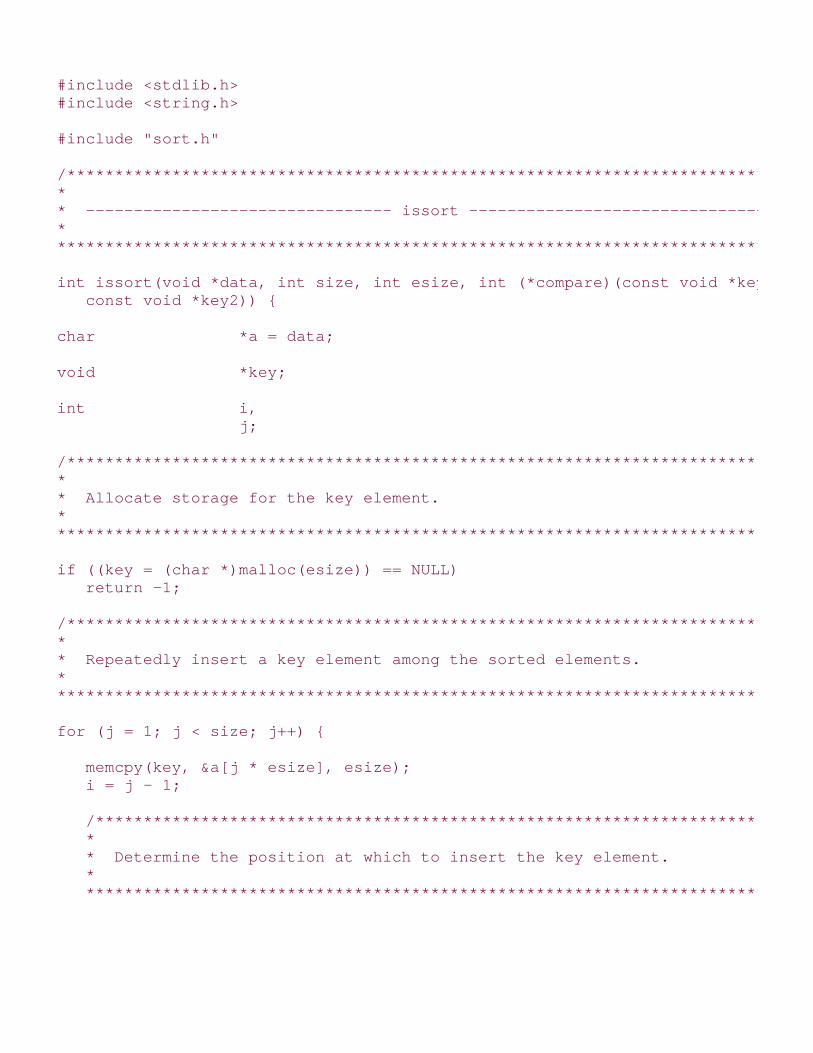
#include <stdlib.h>#include <string.h>
#include "sort.h"
/****************************************************************************** ** -------------------------------- issort -------------------------------- ** ******************************************************************************/
int issort(void *data, int size, int esize, int (*compare)(const void *key1, const void *key2)) {
char *a = data;
void *key;
int i, j;
/****************************************************************************** ** Allocate storage for the key element. ** ******************************************************************************/
if ((key = (char *)malloc(esize)) == NULL) return -1;
/****************************************************************************** ** Repeatedly insert a key element among the sorted elements. ** ******************************************************************************/
for (j = 1; j < size; j++) {
memcpy(key, &a[j * esize], esize); i = j - 1;
/************************************************************************** * * * Determine the position at which to insert the key element. * * * **************************************************************************/

while (i >= 0 && compare(&a[i * esize], key) > 0) {
memcpy(&a[(i + 1) * esize], &a[i * esize], esize); i--;
}
memcpy(&a[(i + 1) * esize], key, esize);
}
/****************************************************************************** ** Free the storage allocated for sorting. ** ******************************************************************************/
free(key);
return 0;
}
Top

Mastering Algorithms with CBy Kyle Loudon
Slots : 1
Table of Contents
Chapter 4. Analysis of Algorithms
Content
4.5 Questions and Answers
Q: From lowest to highest, what is the correct order of the complexities O (n2), O (3n), O (2n), O (n2lg n), O (1), O (n lg n), O (n3), O (n!), O (lg n), O (n)?
A: From lowest to highest, the correct order of these complexities is O (1), O (lg n), O (n), O (n lg n),O (n2), O (n2 lg n), O (n3), O (2n), O (3n), O (n!).
Q: What are the complexities of T1(n) = 3n lg n + lg n; T2(n) = 2n + n3 + 25; and T3(n, k) = k + n,
where k n? From lowest to highest, what is the correct order of the resulting complexities?
A: Using the rules of O -notation, the complexities of T1, T2, and T3 respectively are O (n lg n), O(2n), and O (n). From lowest to highest, the correct order of these complexities is O (n), O (n lg n),and O (2n).
Q: Suppose we have written a procedure to add m square matrices of size n x n. If adding twosquare matrices requires O (n2 ) running time, what is the complexity of this procedure in terms of mand n?
A: To add m matrices of size n x n, we must perform m - 1 additions, each requiring time O (n2).Therefore, the overall running time of this procedure is:
O(m-1)O(n2) = O(m)O(n2) = O(mn2)
Q: Suppose we have two algorithms to solve the same problem. One runs in time T1(n) = 400n,whereas the other runs in time T2(n) = n2. What are the complexities of these two algorithms? Forwhat values of n might we consider using the algorithm with the higher complexity?
A: The complexity of T1 is O (n), and the complexity of T2 is O (n2). However, the algorithm describedby T1 involves such a large constant coefficient for n that when n < 400, the algorithm described byT2 would be preferable. This is a good example of why we sometimes consider other factors besidesthe complexity of an algorithm alone.
Q: How do we account for calls such as memcpy and malloc in analyzing real code? Although thesecalls often depend on the size of the data processed by an algorithm, they are really more of animplementation detail than part of an algorithm itself.
A: Usually calls such as memcpy and malloc are regarded as executing in a constant amount of time.

Generally, they can be expected to execute very efficiently at the machine level regardless of howmuch data they are copying or allocating. Of course, their exact efficiency may depend on thecomputer on which they execute as well as other factors (particularly in the case of malloc, whichdepends on the state of the system at the moment it is called).
Top

Mastering Algorithms with CBy Kyle Loudon
Slots : 1
Table of Contents
Chapter 4. Analysis of Algorithms
Content
4.6 Related Topics
Recurrences
Functions frequently used in the formal analysis of recursive algorithms. Recurrences arerepresented as recursive functions. A recursive function is a function that calls itself (seeChapter 3). Each successive call works on a more refined set of inputs, bringing us closer andcloser to a solution. They are useful in describing the performance of recursive algorithmsbecause they allow us to describe an algorithm's performance in terms of invoking thealgorithm on a more and more refined set of inputs.
Summation formulas
Mathematical formulas useful in simplifying summations that describe the running times ofalgorithms. Summations occur frequently as the result of analyzing iterative control structures.
Q-notation, W-notation, o-notation, and w-notation
Additional notations used to represent information about an algorithm's performance. WhereasO -notation expresses the upper bound of a function within a constant factor, Q -notationexpresses a bound from above and below. W -notation expresses strictly a lower bound within aconstant factor. o -notation and w -notation are analogous to O -notation and W-notation butare more precise. O -notation often is used informally where other notations would be morespecific.
NP-complete problems
A class of problems for which no polynomial-time algorithms are known, but for which no proofexists refuting the possibility either. Thus, NP-completeness has long been one of the mostperplexing vexations in computer science. A polynomial-time algorithm is one whosecomplexity is less than or equal to O (nk), where k is some constant. Many useful anddeceptively difficult problems fall into this class, such as the traveling-salesman problem (seeChapter 16).
Top

Mastering Algorithms with CBy Kyle Loudon
Slots : 1
Table of Contents
Content
Part II: Data StructuresThis part of the book contains seven chapters on data structures. Chapter 5, presents variousforms of linked lists, including singly-linked lists, doubly-linked lists, and circular lists. Chapter6, presents stacks and queues, data structures for sorting and returning data on a last-in, first-out and first-in, first-out order respectively. Chapter 7, presents sets and the fundamentalmathematics describing sets. Chapter 8, presents chained and open-addressed hash tables,including material on how to select a good hash function and how to resolve collisions. Chapter9, presents binary and AVL trees. It also discusses various methods of tree traversal. Chapter10, presents heaps and priority queues, data structures that help to quickly determine thelargest or smallest element in a set of data. Chapter 11, presents graphs and two fundamentalalgorithms from which many graph algorithms are derived: breadth-first and depth-firstsearches.
Top

Mastering Algorithms with CBy Kyle Loudon
Slots : 1
Table of Contents
Part II: Data Structures
Content
Chapter 5. Linked ListsLinked lists are some of the most fundamental data structures. Linked lists consist of a number ofelements grouped, or linked, together in a specific order. They are useful in maintaining collections ofdata, similar to the way that arrays are often used. However, linked lists offer important advantagesover arrays in many cases. Specifically, linked lists are considerably more efficient in performinginsertions and deletions. Linked lists also make use of dynamically allocated storage, which is storageallocated at runtime. Since in many applications the size of the data is not known at compile time,this can be a nice attribute as well.
This chapter covers:
Singly-linked lists
The simplest linked lists, in which elements are linked by a single pointer. This structure allowsthe list to be traversed from its first element to its last.
Doubly-linked lists
Linked lists in which elements are linked by two pointers instead of one. This structure allowsthe list to be traversed both forward and backward.
Circular lists
Linked lists in which the last element is linked to the first instead of being set to NULL. Thisstructure allows the list to be traversed in a circular fashion.
Some applications of linked lists are:
Mailing lists
Lists such as the ones found in email applications. Since it is difficult to predict how long amailing list may be, a mailer might build a linked list of addresses before sending a message.
Scrolled lists
Components found in graphical user interfaces. Often data associated with items in scrolledlists is not displayed. One approach to managing this "hidden" data is to maintain a linked listwherein each element stores the data for one item in the scrolled list.
Polynomials

An important part of mathematics not inherently supported as a datatype by most languages.If we let each element of a linked list store one term, linked lists are useful in representingpolynomials (such as 3x 2 + 2x + 1).
Memory management (illustrated in this chapter)
An important role of operating systems. An operating system must decide how to allocate andreclaim storage for processes running on the system. A linked list can be used to keep track ofportions of memory that are available for allocation.
LISP
An important programming language in artificial intelligence. LISP, an acronym for LIStProcessor, makes extensive use of linked lists in performing symbolic processing.
Linked allocation of files
A type of file allocation that eliminates external fragmentation on a disk but is good only forsequential access. Each block of a file contains a pointer to the file's next block.
Other data structures
Some data structures whose implementations depend on linked lists are stacks, queues, sets,hash tables, and graphs, all of which are presented in this book.
Top

Mastering Algorithms with CBy Kyle Loudon
Slots : 1
Table of Contents
Chapter 5. Linked Lists
Content
5.1 Description of Linked Lists
Singly-linked lists , usually simply called linked lists, are composed of individual elements, each linkedby a single pointer. Each element consists of two parts: a data member and a pointer, called the nextpointer. Using this two-member structure, a linked list is formed by setting the next pointer of eachelement to point to the element that follows it (see Figure 5.1). The next pointer of the last elementis set to NULL, a convenient sentinel marking the end of the list. The element at the start of the list isits head; the element at the end of the list is its tail.
To access an element in a linked list, we start at the head of the list and use the next pointers ofsuccessive elements to move from element to element until the desired element is reached. Withsingly-linked lists, the list can be traversed in only one direction—from head to tail—because eachelement contains no link to its predecessor. Therefore, if we start at the head and move to someelement, and then wish to access an element preceding it, we must start over at the head (althoughsometimes we can anticipate the need to know an element and save a pointer to it). Often thisweakness is not a concern. When it is, we use a doubly-linked list or circular list.
Conceptually, one thinks of a linked list as a series of contiguous elements. However, because theseelements are allocated dynamically (using malloc in C), it is important to remember that, in actuality,they are usually scattered about in memory (see Figure 5.2). The pointers from element to elementtherefore are the only means by which we can ensure that all elements remain accessible. With thisin mind, we will see later that special care is required when it comes to maintaining the links. If wemistakenly drop one link, it becomes impossible to access any of the elements from that point on inthe list. Thus, the expression "You are only as strong as your weakest link" is particularly fitting forlinked lists.
Figure 5.1. Elements linked together to form a linked list
Figure 5.2. Elements of a linked list linked but scattered about an

address space
Top

Mastering Algorithms with CBy Kyle Loudon
Slots : 1
Table of Contents
Chapter 5. Linked Lists
Content
5.2 Interface for Linked Lists
list_init
void list_init(List *list, void (*destroy)(void *data));
Return Value
None.
Description
Initializes the linked list specified by list. This operation must be called for a linked list before thelist can be used with any other operation. The destroy argument provides a way to freedynamically allocated data when list_destroy is called. For example, if the list contains datadynamically allocated using malloc, destroy should be set to free to free the data as the linked listis destroyed. For structured data containing several dynamically allocated members, destroyshould be set to a user-defined function that calls free for each dynamically allocated member as wellas for the structure itself. For a linked list containing data that should not be freed, destroy shouldbe set to NULL.
Complexity
O (1)
list_destroy
void list_destroy(List *list);
Return Value

None.
Description
Destroys the linked list specified by list. No other operations are permitted after callinglist_destroy unless list_init is called again. The list_destroy operation removes all elements from alinked list and calls the function passed as destroy to list_init once for each element as it isremoved, provided destroy was not set to NULL.
Complexity
O (n), where n is the number of elements in the linked list.
list_ins_next
int list_ins_next(List *list, ListElmt *element, const void *data);
Return Value
0 if inserting the element is successful, or -1 otherwise.
Description
Inserts an element just after element in the linked list specified by list. If element is NULL, thenew element is inserted at the head of the list. The new element contains a pointer to data, so thememory referenced by data should remain valid as long as the element remains in the list. It is theresponsibility of the caller to manage the storage associated with data.
Complexity
O (1)
list_rem_next
int list_rem_next(List *list, ListElmt *element, void **data);
Return Value
0 if removing the element is successful, or -1 otherwise.

Description
Removes the element just after element from the linked list specified by list. If element isNULL, the element at the head of the list is removed. Upon return, data points to the data stored inthe element that was removed. It is the responsibility of the caller to manage the storage associatedwith the data.
Complexity
O (1)
list_size
int list_size(const List *list);
Return Value
Number of elements in the list.
Description
Macro that evaluates to the number of elements in the linked list specified by list.
Complexity
O (1)
list_head
ListElmt *list_head(const List *list);
Return Value
Element at the head of the list.
Description
Macro that evaluates to the element at the head of the linked list specified by list.
Complexity

O (1)
list_tail
ListElmt *list_tail(const List *list);
Return Value
Element at the tail of the list.
Description
Macro that evaluates to the element at the tail of the linked list specified by list.
Complexity
O (1)
list_is_head
int list_is_head(const ListElmt *element);
Return Value
1 if the element is at the head of the list, or otherwise.
Description
Macro that determines whether the element specified as element is at the head of a linked list.
Complexity
O (1)
list_is_tail
int list_is_tail(const ListElmt *element);
Return Value

1 if the element is at the tail of the list, or otherwise.
Description
Macro that determines whether the element specified as element is at the tail of a linked list.
Complexity
O (1)
list_data
void *list_data(const ListElmt *element);
Return Value
Data stored in the element.
Description
Macro that evaluates to the data stored in the element of a linked list specified by element.
Complexity
O (1)
list_next
ListElmt *list_next(const ListElmt *element);
Return Value
Element following the specified element.
Description
Macro that evaluates to the element of a linked list following the element specified by element.
Complexity

O (1)
Top

Mastering Algorithms with CBy Kyle LoudonSlots : 1Table of ContentsChapter 5. Linked Lists
Content
5.3 Implementation and Analysis of Linked Lists
Recall that each element of a linked list consists of two parts: a data member and a pointer to the next
element in the list. The structure ListElmt represents an individual element of a linked list (see
Example 5.1 ). As you would expect, this structure has two members that correspond to those just
mentioned. The structure List is the linked list data structure (see Example 5.1 ). This structure consists
of five members: size is the number of elements in the list, match is a member not used by linked lists
but by datatypes that will be derived later from linked lists, destroy is the encapsulated destroy function
passed to list_init , head is a pointer to the first of the linked elements, and tail is a pointer to the tail
element.
Example 5.1. Header for the Linked List Abstract Datatype
/****************************************************************************** ** -------------------------------- list.h -------------------------------- ** ******************************************************************************/
#ifndef LIST_H#define LIST_H
#include <stdlib.h>
/****************************************************************************** ** Define a structure for linked list elements. ** ******************************************************************************/

typedef struct ListElmt_ {
void *data;struct ListElmt_ *next;
} ListElmt;
/****************************************************************************** ** Define a structure for linked lists. ** ******************************************************************************/
typedef struct List_ {
int size;
int (*match)(const void *key1, const void *key2);void (*destroy)(void *data);
ListElmt *head;ListElmt *tail;
} List;
/****************************************************************************** ** --------------------------- Public Interface --------------------------- ** ******************************************************************************/
void list_init(List *list, void (*destroy)(void *data));
void list_destroy(List *list);
int list_ins_next(List *list, ListElmt *element, const void *data);
int list_rem_next(List *list, ListElmt *element, void **data);
#define list_size(list) ((list)->size)
#define list_head(list) ((list)->head)
#define list_tail(list) ((list)->tail)
#define list_is_head(list, element) ((element) == (list)->head ? 1 : 0)
#define list_is_tail(element) ((element)->next == NULL ? 1 : 0)
#define list_data(element) ((element)->data)
#define list_next(element) ((element)->next)
#endif
5.3.1 list_init
The list_init operation initializes a linked list so that it can be used in other operations (see Example 5.2 ).
Initializing a linked list is a simple operation in which the size member of the list is set to 0, the
destroy member to destroy , and the head and tail pointers to NULL.
The runtime complexity of list_init is O (1) because all of the steps in initializing a linked list run in aconstant amount of time.
5.3.2 list_destroy
The list_destroy operation destroys a linked list (see Example 5.2 ). Primarily this means removing all
elements from the list. The function passed as destroy to list_init is called once for each element as it is
removed, provided destroy was not set to NULL.
The runtime complexity of list_destroy is O (n ), where n is the number of elements in the list. This isbecause the O (1) operation list_rem_next must be called once for each element.
5.3.3 list_ins_next
The list_ins_next operation inserts an element into a linked list just after a specified element (see Example5.2 ). The call sets the new element to point to the data passed by the caller. The actual process ofinserting the new element into the list is a simple one, but it does require some care. There are two casesto consider: insertion at the head of the list and insertion elsewhere.
Generally, to insert an element into a linked list, we set the next pointer of the new element to point to
the element it is going to precede, and we set the next pointer of the element that will precede the new
element to point to the new element (see Figure 5.3 ). However, when inserting at the head of a list, there
is no element that will precede the new element. Thus, in this case, we set the next pointer of the new
element to the current head of the list, then reset the head of the list to point to the new element. Recall
from the interface design in the previous section that passing NULL for element indicates that the new
element should be inserted at the head. In addition to these tasks, whenever we insert an element at the
tail of the list, we must update the tail member of the list data structure to point to the new tail. Last,
we update the size of the list by incrementing its size member.
Figure 5.3. Inserting an element into a linked list

The runtime complexity of list_ins_next is O (1) because all of the steps in inserting an element into alinked list run in a constant amount of time.
5.3.4 list_rem_next
The list_rem_next operation removes from a linked list the element just after a specified element (seeExample 5.2 ). The reasons for removing the element just after, as opposed to the element itself, arediscussed in the questions and answers at the end of the chapter. As with inserting an element, this callrequires consideration of two cases: removing an element from the head of the list and removing oneelsewhere.
The actual process of removing the element from the list is a simple one, but it too requires some care (see
Figure 5.4 ). Generally, to remove an element from a linked list, we set the next pointer of the element
preceding the one being removed to point to the element after the element being removed. However, whenremoving an element from the head of a list, there is no element that precedes the element beingremoved. Thus, in this case, we set the head of the list to point to the element after the one being
removed. As with insertion, NULL serves nicely as a sentinel passed in element to indicate that the
element at the head of the list should be removed. In addition to these tasks, whenever we remove the
element at the tail of the list, we must update the tail member of the list data structure to point to the
new tail, or to NULL if removing the element has caused the list to become empty. Last, we update the size
of the list by decreasing the size member by 1. Upon return, data points to the data from the element
removed.
Figure 5.4. Removing an element from a linked list

The runtime complexity of list_rem_next is O (1) because all of the steps in removing an element from alinked list run in a constant amount of time.
5.3.5 list_size, list_head, list_tail, list_is_tail,list_data, and list_next
These macros implement some of the simpler linked list operations (see Example 5.1 ). Generally, they
provide an interface for accessing and testing members of the List and ListElmt structures.
The runtime complexity of these operations is O (1) because accessing and testing members of a structureare simple tasks that run in a constant amount of time.
Example 5.2. Implementation of the Linked List Abstract Datatype
/****************************************************************************** ** -------------------------------- list.c -------------------------------- ** ******************************************************************************/
#include <stdlib.h>#include <string.h>
#include "list.h"
/****************************************************************************** ** ------------------------------- list_init ------------------------------ ** ******************************************************************************/
void list_init(List *list, void (*destroy)(void *data)) {
/****************************************************************************** ** Initialize the list. ** ******************************************************************************/
list->size = 0;list->destroy = destroy;list->head = NULL;list->tail = NULL;
return;
}

/****************************************************************************** ** ----------------------------- list_destroy ----------------------------- ** ******************************************************************************/
void list_destroy(List *list) {
void *data;
/****************************************************************************** ** Remove each element. ** ******************************************************************************/
while (list_size(list) > 0) {
if (list_rem_next(list, NULL, (void **)&data) == 0 && list->destroy != NULL) {
/*********************************************************************** * * * Call a user-defined function to free dynamically allocated data. * * * ***********************************************************************/
list->destroy(data);
}
}
/****************************************************************************** ** No operations are allowed now, but clear the structure as a precaution. ** ******************************************************************************/
memset(list, 0, sizeof(List));
return;
}
/*****************************************************************************

* ** ----------------------------- list_ins_next ---------------------------- ** ******************************************************************************/
int list_ins_next(List *list, ListElmt *element, const void *data) {
ListElmt *new_element;
/****************************************************************************** ** Allocate storage for the element. ** ******************************************************************************/
if ((new_element = (ListElmt *)malloc(sizeof(ListElmt))) == NULL) return -1;
/****************************************************************************** ** Insert the element into the list. ** ******************************************************************************/
new_element->data = (void *)data;
if (element == NULL) {
/************************************************************************** * * * Handle insertion at the head of the list. * * * **************************************************************************/
if (list_size(list) == 0) list->tail = new_element;
new_element->next = list->head; list->head = new_element;
}
else {
/************************************************************************** * *

* Handle insertion somewhere other than at the head. * * * **************************************************************************/
if (element->next == NULL) list->tail = new_element;
new_element->next = element->next; element->next = new_element;
}
/****************************************************************************** ** Adjust the size of the list to account for the inserted element. ** ******************************************************************************/
list->size++;
return 0;
}
/****************************************************************************** ** ----------------------------- list_rem_next ---------------------------- ** ******************************************************************************/
int list_rem_next(List *list, ListElmt *element, void **data) {
ListElmt *old_element;
/****************************************************************************** ** Do not allow removal from an empty list. ** ******************************************************************************/
if (list_size(list) == 0) return -1;
/****************************************************************************** ** Remove the element from the list. *

* ******************************************************************************/
if (element == NULL) {
/************************************************************************** * * * Handle removal from the head of the list. * * * **************************************************************************/
*data = list->head->data; old_element = list->head; list->head = list->head->next;
if (list_size(list) == 1) list->tail = NULL;
}
else {
/************************************************************************** * * * Handle removal from somewhere other than the head. * * * **************************************************************************/
if (element->next == NULL) return -1;
*data = element->next->data; old_element = element->next; element->next = element->next->next;
if (element->next == NULL) list->tail = element;
}
/****************************************************************************** ** Free the storage allocated by the abstract datatype. ** ******************************************************************************/

free(old_element);
/****************************************************************************** ** Adjust the size of the list to account for the removed element. ** ******************************************************************************/
list->size--;
return 0;
}
Top

Mastering Algorithms with CBy Kyle LoudonSlots : 1Table of ContentsChapter 5. Linked Lists
Content
5.4 Linked List Example: Frame Management
An interesting application of linked lists is found in the way some systems support virtual memory . Virtualmemory is a mapping of address space that allows a process (a running program) to execute without beingcompletely in physical memory , the real memory of the system. One advantage of this is that a processcan make use of an address space that is much larger than that which the physical memory of the systemwould allow otherwise. Another advantage is that multiple processes can share the memory of the systemwhile running concurrently.
A process running in virtual memory deals with virtual addresses . These are addresses that seem likephysical addresses to the process, but that the system must translate before using. Address translationtakes place using a page table and is fast due to dedicated hardware. Each process has its own page tablethat maps pages of its virtual address space to frames in physical memory. When a process references aparticular virtual address, the appropriate entry in its page table is inspected to determine in which physicalframe the page resides (see Figure 5.5 ). When a process references a virtual address not yet in a frame, apage fault occurs and a frame is allocated in physical memory. Why pages of a process are removed fromphysical memory is another matter. One occasion for removing a page, however, is when a page isaccessed infrequently relative to other pages and its frame is needed elsewhere.
Figure 5.5. A virtual memory system
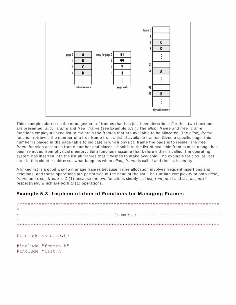
This example addresses the management of frames that has just been described. For this, two functionsare presented, alloc_ frame and free_ frame (see Example 5.3 ). The alloc_ frame and free_ framefunctions employ a linked list to maintain the frames that are available to be allocated. The alloc_ framefunction retrieves the number of a free frame from a list of available frames. Given a specific page, thisnumber is placed in the page table to indicate in which physical frame the page is to reside. The free_frame function accepts a frame number and places it back into the list of available frames once a page hasbeen removed from physical memory. Both functions assume that before either is called, the operatingsystem has inserted into the list all frames that it wishes to make available. The example for circular listslater in this chapter addresses what happens when alloc_ frame is called and the list is empty.
A linked list is a good way to manage frames because frame allocation involves frequent insertions anddeletions, and these operations are performed at the head of the list. The runtime complexity of both alloc_frame and free_ frame is O (1) because the two functions simply call list_rem_next and list_ins_nextrespectively, which are both O (1) operations.
Example 5.3. Implementation of Functions for Managing Frames
/****************************************************************************** ** ------------------------------- frames.c ------------------------------- ** ******************************************************************************/
#include <stdlib.h>
#include "frames.h"#include "list.h"
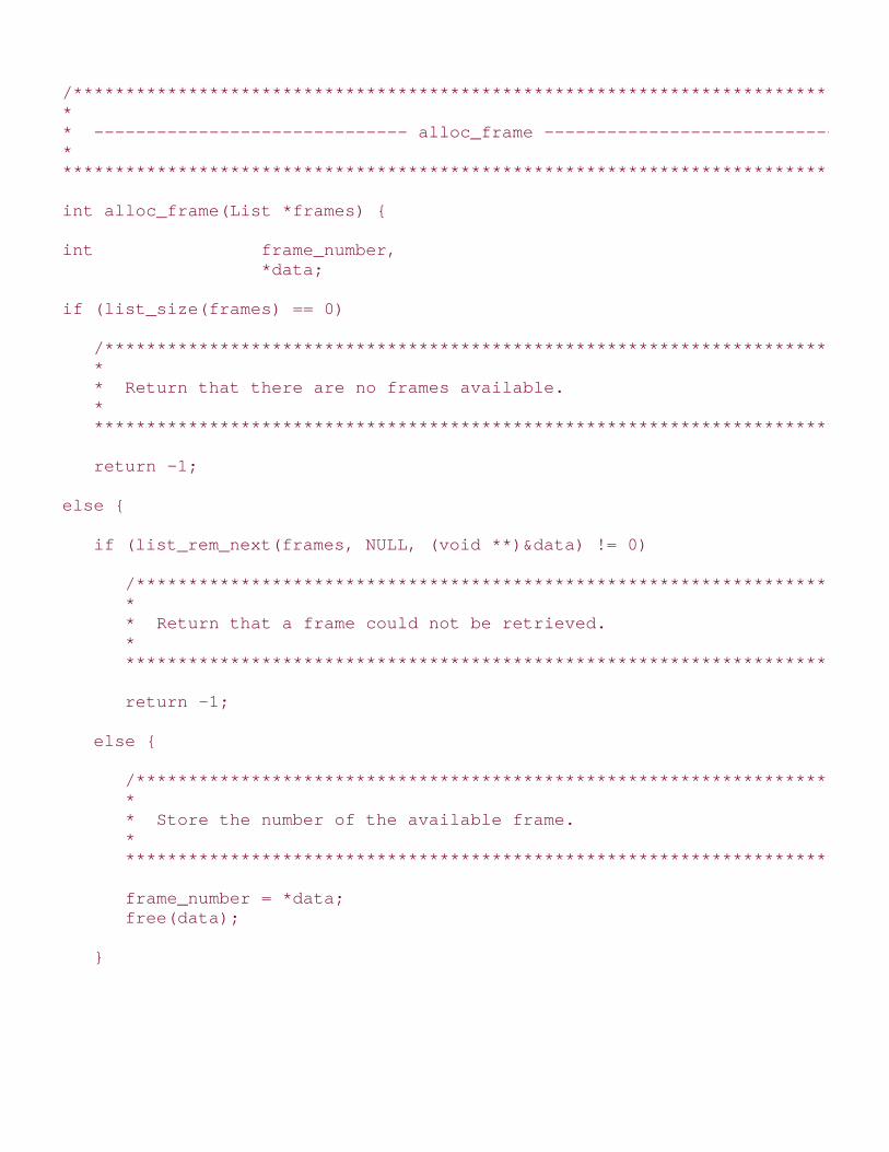
/****************************************************************************** ** ------------------------------ alloc_frame ----------------------------- ** ******************************************************************************/
int alloc_frame(List *frames) {
int frame_number, *data;
if (list_size(frames) == 0)
/************************************************************************** * * * Return that there are no frames available. * * * **************************************************************************/
return -1;
else {
if (list_rem_next(frames, NULL, (void **)&data) != 0)
/*********************************************************************** * * * Return that a frame could not be retrieved. * * * ***********************************************************************/
return -1;
else {
/*********************************************************************** * * * Store the number of the available frame. * * * ***********************************************************************/
frame_number = *data; free(data);
}

}
return frame_number;
}
/****************************************************************************** ** ------------------------------ free_frame ------------------------------ ** ******************************************************************************/
int free_frame(List *frames, int frame_number) {
int *data;
/****************************************************************************** ** Allocate storage for the frame number. ** ******************************************************************************/
if ((data = (int *)malloc(sizeof(int))) == NULL) return -1;
/****************************************************************************** ** Put the frame back in the list of available frames. ** ******************************************************************************/
*data = frame_number;
if (list_ins_next(frames, NULL, data) != 0) return -1;
return 0;
}
Top

Mastering Algorithms with CBy Kyle Loudon
Slots : 1
Table of Contents
Chapter 5. Linked Lists
Content
5.5 Description of Doubly-Linked Lists
Doubly-linked lists , as their name implies, are composed of elements linked by two pointers. Eachelement of a doubly-linked list consists of three parts: in addition to the data and the next pointer,each element includes a pointer to the previous element, called the prev pointer. A doubly-linked listis formed by composing a number of elements so that the next pointer of each element points to theelement that follows it, and the prev pointer points to the element preceding it. To mark the headand tail of the list, we set the prev pointer of the first element and the next pointer of the lastelement to NULL.
To traverse backward through a doubly-linked list, we use the prev pointers of consecutive elementsin the tail-to-head direction. Thus, for the cost of an additional pointer for each element, a doubly-linked list offers greater flexibility than a singly-linked list in moving about the list. This can be usefulwhen we know something about where an element might be stored in the list and can choose wiselyhow to move to it. For example, one flexibility that doubly-linked lists provide is a more intuitivemeans of removing an element than singly-linked lists.
Top

Mastering Algorithms with CBy Kyle Loudon
Slots : 1
Table of Contents
Chapter 5. Linked Lists
Content
5.6 Interface for Doubly-Linked Lists
dlist_init
void dlist_init(DList *list, void (*destroy)(void *data));
Return Value
None.
Description
Initializes the doubly-linked list specified by list. This operation must be called for a doubly-linked listbefore the list can be used with any other operation. The destroy argument provides a way to freedynamically allocated data when dlist_destroy is called. It works in a manner similar to that describedfor list_destroy. For a doubly-linked list containing data that should not be freed, destroy should beset to NULL.
Complexity
O (1)
dlist_destroy
void dlist_destroy(DList *list);
Return Value
None.

Description
Destroys the doubly-linked list specified by list. No other operations are permitted after callingdlist_destroy unless dlist_init is called again. The dlist_destroy operation removes all elements from adoubly-linked list and calls the function passed as destroy to dlist_init once for each element as it isremoved, provided destroy was not set to NULL.
Complexity
O (n), where n is the number of elements in the doubly-linked list.
dlist_ins_next
int dlist_ins_next(DList *list, DListElmt *element, const void *data);
Return Value
0 if inserting the element is successful, or -1 otherwise.
Description
Inserts an element just after element in the doubly-linked list specified by list. When inserting intoan empty list, element may point anywhere, but should be NULL to avoid confusion. The new elementcontains a pointer to data, so the memory referenced by data should remain valid as long as theelement remains in the list. It is the responsibility of the caller to manage the storage associated withdata.
Complexity
O (1)
dlist_ins_prev
int dlist_ins_prev(DList *list, DListElmt *element, const void *data);
Return Value
0 if inserting the element is successful, or -1 otherwise.
Description

Inserts an element just before element in the doubly-linked list specified by list. When inserting intoan empty list, element may point anywhere, but should be NULL to avoid confusion. The new elementcontains a pointer to data, so the memory referenced by data should remain valid as long as theelement remains in the list. It is the responsibility of the caller to manage the storage associated withdata.
Complexity
O (1)
dlist_remove
int dlist_remove(DList *list, DListElmt *element, void **data);
Return Value
0if removing the element is successful, or -1 otherwise.
Description
Removes the element specified as element from the doubly-linked list specified by list. Upon return,data points to the data stored in the element that was removed. It is the responsibility of the caller tomanage the storage associated with the data.
Complexity
O (1)
dlist_size
int dlist_size(const DList *list);
Return Value
Number of elements in the list.
Description
Macro that evaluates to the number of elements in the doubly-linked list specified by list.
Complexity

O (1)
dlist_head
DListElmt *dlist_head(const DList *list);
Return Value
Element at the head of the list.
Description
Macro that evaluates to the element at the head of the doubly-linked list specified by list.
Complexity
O (1)
dlist_tail
DListElmt *dlist_tail(const DList *list);
Return Value
Element at the tail of the list.
Description
Macro that evaluates to the element at the tail of the doubly-linked list specified by list.
Complexity
O (1)
dlist_is_head
int dlist_is_head(const DListElmt *element);
Return Value

1 if the element is at the head of the list, or 0 otherwise.
Description
Macro that determines whether the element specified as element is at the head of a doubly-linked list.
Complexity
O (1)
dlist_is_tail
int dlist_is_tail(const DListElmt *element);
Return Value
1 if the element is at the tail of the list, or otherwise.
Description
Macro that determines whether the element specified as element is at the tail of a doubly-linked list.
Complexity
O (1)
dlist_data
void *dlist_data(const DListElmt *element);
Return Value
Data stored in the element.
Description
Macro that evaluates to the data stored in the element of a doubly-linked list specified by element.
Complexity

O (1)
dlist_next
DListElmt *dlist_next(const DListElmt *element);
Return Value
Element following the specified element.
Description
Macro that evaluates to the element of a doubly-linked list following the element specified by element.
Complexity
O (1)
dlist_prev
DListElmt *dlist_prev(const DListElmt *element);
Return Value
Element preceding the specified element.
Description
Macro that evaluates to the element of a doubly-linked list preceding the element specified byelement.
Complexity
O (1)
Top

Mastering Algorithms with CBy Kyle LoudonSlots : 1Table of ContentsChapter 5. Linked Lists
Content
5.7 Implementation and Analysis of Doubly Linked Lists
Recall that each element of a doubly-linked list consists of three parts: a data member, a pointer to the
next element, and a pointer to the previous element. The structure DListElmt represents an individual
element of a doubly-linked list (see Example 5.4 ). As you would expect, this structure has three members
corresponding to those just mentioned. The structure DList is the doubly-linked list data structure (see
Example 5.4 ). This structure has members analogous to the ones used for singly-linked lists.
Example 5.4. Header for the Doubly-Linked List Abstract Datatype
/****************************************************************************** ** ------------------------------- dlist.h -------------------------------- ** ******************************************************************************/
#ifndef DLIST_H#define DLIST_H
#include <stdlib.h>
/****************************************************************************** ** Define a structure for doubly-linked list elements. ** ******************************************************************************/
typedef struct DListElmt_ {

void *data;struct DListElmt_ *prev;struct DListElmt_ *next;
} DListElmt;
/****************************************************************************** ** Define a structure for doubly-linked lists. ** ******************************************************************************/
typedef struct DList_ {
int size;
int (*match)(const void *key1, const void *key2);void (*destroy)(void *data);
DListElmt *head;DListElmt *tail;
} DList;
/****************************************************************************** ** --------------------------- Public Interface --------------------------- ** ******************************************************************************/
void dlist_init(DList *list, void (*destroy)(void *data));
void dlist_destroy(DList *list);
int dlist_ins_next(DList *list, DListElmt *element, const void *data);
int dlist_ins_prev(DList *list, DListElmt *element, const void *data);
int dlist_remove(DList *list, DListElmt *element, void **data);
#define dlist_size(list) ((list)->size)
#define dlist_head(list) ((list)->head)
#define dlist_tail(list) ((list)->tail)

#define dlist_is_head(element) ((element)->prev == NULL ? 1 : 0)
#define dlist_is_tail(element) ((element)->next == NULL ? 1 : 0)
#define dlist_data(element) ((element)->data)
#define dlist_next(element) ((element)->next)
#define dlist_prev(element) ((element)->prev)
#endif
5.7.1 dlist_init
The dlist_init operation initializes a doubly-linked list so that it can be used in other operations (seeExample 5.5 ). Initialization is the same as with a singly-linked list.
The runtime complexity of dlist_init is O (1) because all of the steps in initializing a doubly-linked list run ina constant amount of time.
5.7.2 dlist_destroy
The dlist_destroy operation destroys a doubly-linked list (see Example 5.5 ). Primarily this means removing
all elements from the list. The function passed as destroy to dlist_init is called once for each element as
it is removed, provided destroy was not set to NULL.
The runtime complexity of dlist_destroy is O (n ), where n is the number of elements in the list. This isbecause the O (1) operation dlist_remove must be called once for each element.
5.7.3 dlist_ins_next
The dlist_ins_next operation inserts an element into a doubly-linked list just after a specified element (seeExample 5.5 ). Inserting an element in a doubly-linked list is similar to inserting one in a singly-linked list.
The primary difference is that in addition to managing the next pointers, we must manage the prevpointers to keep the list linked properly in the reverse direction (see Figure 5.6 ).
Figure 5.6. Inserting an element into a doubly-linked list with dlist_ins_next

The runtime complexity of dlist_ins_next is O (1) because all of the steps in inserting an element into adoubly-linked list run in a constant amount of time.
5.7.4 dlist_ins_ prev
The dlist_ins_ prev operation inserts an element into a doubly-linked list just before a specified element(see Example 5.5 ). Inserting an element in a doubly-linked list is similar to inserting one in a singly-linked
list. As with dlist_ins_next , the primary difference is that in addition to managing the next pointers, we
must manage the prev pointers to keep the list linked properly in the reverse direction.
The runtime complexity of dlist_ins_prev is O (1) because all of the steps in inserting an element into adoubly-linked list run in a constant amount of time.
5.7.5 dlist_remove
The dlist_remove operation removes a specified element from a doubly-linked list (see Example 5.5 ). The
primary difference from a singly-linked list is that in addition to managing the next pointers, we must
manage the prev pointers to keep the list linked properly in the reverse direction. Another difference is
that in a doubly-linked list, it is possible to remove the specified element rather than the one just after it

because there is a pointer back to the previous element.
The runtime complexity of dlist_remove is O (1) because all of the steps in removing an element from adoubly-linked list run in a constant amount of time.
5.7.6 dlist_size, dlist_head, dlist_tail, dlist_is_head, dlist_is_tail, dlist_data,dlist_next, and dlist_ prev
These macros implement some of the simpler doubly-linked list operations (see Example 5.4 ). Generally,
they provide an interface for accessing and testing members of the DList and DListElmt structures.
The runtime complexity of these operations is O (1) because accessing and testing members of a structureare simple tasks that run in a constant amount of time.
Example 5.5. Implementation of the Doubly-Linked List Abstract Datatype
/****************************************************************************** ** ------------------------------- dlist.c -------------------------------- ** ******************************************************************************/
#include <stdlib.h>#include <string.h>
#include "dlist.h"
/****************************************************************************** ** ------------------------------ dlist_init ------------------------------ ** ******************************************************************************/
void dlist_init(DList *list, void (*destroy)(void *data)) {
/****************************************************************************** ** Initialize the list. ** ******************************************************************************/
list->size = 0;list->destroy = destroy;list->head = NULL;list->tail = NULL;

return;
}
/****************************************************************************** ** ---------------------------- dlist_destroy ----------------------------- ** ******************************************************************************/
void dlist_destroy(DList *list) {
void *data;
/****************************************************************************** ** Remove each element. ** ******************************************************************************/
while (dlist_size(list) > 0) {
if (dlist_remove(list, dlist_tail(list), (void **)&data) == 0 && list-> destroy != NULL) {
/*********************************************************************** * * * Call a user-defined function to free dynamically allocated data. * * * ***********************************************************************/
list->destroy(data);
}
}
/****************************************************************************** ** No operations are allowed now, but clear the structure as a precaution. ** ******************************************************************************/
memset(list, 0, sizeof(DList));
return;

}
/****************************************************************************** ** ---------------------------- dlist_ins_next ---------------------------- ** ******************************************************************************/
int dlist_ins_next(DList *list, DListElmt *element, const void *data) {
DListElmt *new_element;
/****************************************************************************** ** Do not allow a NULL element unless the list is empty. ** ******************************************************************************/
if (element == NULL && dlist_size(list) != 0) return -1;
/****************************************************************************** ** Allocate storage for the element. ** ******************************************************************************/
if ((new_element = (DListElmt *)malloc(sizeof(DListElmt))) == NULL) return -1;
/****************************************************************************** ** Insert the new element into the list. ** ******************************************************************************/
new_element->data = (void *)data;
if (dlist_size(list) == 0) {
/************************************************************************** * * * Handle insertion when the list is empty. * * * **************************************************************************/

list->head = new_element; list->head->prev = NULL; list->head->next = NULL; list->tail = new_element;
}
else {
/************************************************************************** * * * Handle insertion when the list is not empty. * * * **************************************************************************/
new_element->next = element->next; new_element->prev = element;
if (element->next == NULL) list->tail = new_element; else element->next->prev = new_element;
element->next = new_element;
}
/****************************************************************************** ** Adjust the size of the list to account for the inserted element. ** ******************************************************************************/
list->size++;
return 0;
}
/****************************************************************************** ** ---------------------------- dlist_ins_prev ---------------------------- ** ******************************************************************************/

int dlist_ins_prev(DList *list, DListElmt *element, const void *data) {
DListElmt *new_element;
/****************************************************************************** ** Do not allow a NULL element unless the list is empty. ** ******************************************************************************/
if (element == NULL && dlist_size(list) != 0) return -1;
/****************************************************************************** ** Allocate storage to be managed by the abstract datatype. ** ******************************************************************************/
if ((new_element = (DListElmt *)malloc(sizeof(DListElmt))) == NULL) return -1;
/****************************************************************************** ** Insert the new element into the list. ** ******************************************************************************/
new_element->data = (void *)data;
if (dlist_size(list) == 0) {
/************************************************************************** * * * Handle insertion when the list is empty. * * * **************************************************************************/
list->head = new_element; list->head->prev = NULL; list->head->next = NULL; list->tail = new_element;
}

else {
/************************************************************************** * * * Handle insertion when the list is not empty. * * * **************************************************************************/
new_element->next = element; new_element->prev = element->prev;
if (element->prev == NULL) list->head = new_element; else element->prev->next = new_element;
element->prev = new_element;
}
/****************************************************************************** ** Adjust the size of the list to account for the new element. ** ******************************************************************************/
list->size++;
return 0;
}
/****************************************************************************** ** ----------------------------- dlist_remove ----------------------------- ** ******************************************************************************/
int dlist_remove(DList *list, DListElmt *element, void **data) {
/****************************************************************************** ** Do not allow a NULL element or removal from an empty list. ** ******************************************************************************/

if (element == NULL || dlist_size(list) == 0) return -1;
/****************************************************************************** ** Remove the element from the list. ** ******************************************************************************/
*data = element->data;
if (element == list->head) {
/************************************************************************** * * * Handle removal from the head of the list. * * * **************************************************************************/
list->head = element->next;
if (list->head == NULL) list->tail = NULL; else element->next->prev = NULL;
}
else {
/************************************************************************** * * * Handle removal from other than the head of the list. * * * **************************************************************************/
element->prev->next = element->next;
if (element->next == NULL) list->tail = element->prev; else element->next->prev = element->prev;
}
/*****************************************************************************

* ** Free the storage allocated by the abstract datatype. ** ******************************************************************************/
free(element);
/****************************************************************************** ** Adjust the size of the list to account for the removed element. ** ******************************************************************************/
list->size--;
return 0;
}
Top

Mastering Algorithms with CBy Kyle Loudon
Slots : 1
Table of Contents
Chapter 5. Linked Lists
Content
5.8 Description of Circular Lists
The circular list is another form of linked list that provides additional flexibility in traversing elements.A circular list may be singly-linked or doubly-linked, but its distinguishing feature is that it has no tail.In a circular list, the next pointer of the last element points back to its first element rather than toNULL. In the case of a doubly-linked circular list, the prev pointer of the first element is set to pointto the last element as well.
Whether dealing with a singly-linked or doubly-linked circular list, we never need to worry aboutreaching an element from which we can traverse no further as we move from element to element.Instead, the traversal simply continues back to the first element, or, in the case of a doubly-linkedcircular list, back to the last element. Traversing a list in this manner produces a circular pattern (seeFigure 5.7), hence its name.
Figure 5.7. Elements linked together to form a circular list
The circular list presented in the following sections is a singly-linked circular list. Therefore, we areconcerned only with maintaining a link from the last element back to the first element. In practice,whether to make use of a singly-linked circular list or one that is doubly-linked depends on the samereasoning presented earlier for choosing between singly-linked and doubly-linked lists that are notcircular.
Top

Mastering Algorithms with CBy Kyle Loudon
Slots : 1
Table of Contents
Chapter 5. Linked Lists
Content
5.9 Interface for Circular Lists
clist_init
void clist_init(CList *list, void (*destroy)(void *data));
Return Value
None.
Description
Initializes the circular list specified by list. This operation must be called for a circular list before thelist can be used with any other operation. The destroy argument provides a way to free dynamicallyallocated data when clist_destroy is called. It works in a manner similar to that described forlist_destroy. For a circular list containing data that should not be freed, destroy should be set toNULL.
Complexity
O (1)
clist_destroy
void clist_destroy(CList *list);
Return Value
None.

Description
Destroys the circular list specified by list. No other operations are permitted after calling clist_destroyunless clist_init is called again. The clist_destroy operation removes all elements from a circular list andcalls the function passed as destroy to clist_init once for each element as it is removed, provideddestroy was not set to NULL.
Complexity
O (n), where n is the number of elements in the circular list.
clist_ins_next
int clist_ins_next(CList *list, CListElmt *element, const void *data);
Return Value
0if inserting the element is successful, or -1 otherwise.
Description
Inserts an element just after element in the circular list specified by list. When inserting into anempty list, element may point anywhere but should be NULL to avoid confusion. The new elementcontains a pointer to data, so the memory referenced by data should remain valid as long as theelement remains in the list. It is the responsibility of the caller to manage the storage associated withdata.
Complexity
O (1)
clist_rem_next
int clist_rem_next(CList *list, CListElmt *element, void **data);
Return Value
0if removing the element is successful, or -1 otherwise.
Description

Removes the element just after element from the circular list specified by list. Upon return, datapoints to the data stored in the element that was removed. It is the responsibility of the caller tomanage the storage associated with the data.
Complexity
O (1)
clist_size
int clist_size(const CList *list);
Return Value
Number of elements in the list.
Description
Macro that evaluates to the number of elements in the circular list specified by list.
Complexity
O (1)
clist_head
CListElmt *clist_head(const CList *list);
Return Value
Element at the head of the list.
Description
Macro that evaluates to the element at the head of the circular list specified by list.
Complexity
O (1)

clist_data
void *clist_data(const CListElmt *element);
Return Value
Data stored in the element.
Description
Macro that evaluates to the data stored in the element of a circular list specified by element.
Complexity
O (1)
clist_next
CListElmt *clist_next(const CListElmt *element);
Return Value
Element following the specified element.
Description
Macro that evaluates to the element of a circular list following the element specified by element.
Complexity
O (1)
Top

Mastering Algorithms with CBy Kyle LoudonSlots : 1Table of ContentsChapter 5. Linked Lists
Content
5.10 Implementation and Analysis of Circular Lists
As with a singly-linked list, each element of a circular list consists of two parts: a data member and a
pointer to the next element. The structure CListElmt represents an individual element of a circular list
(see Example 5.6 ). As you would expect, this structure has two members corresponding to those just
mentioned. The structure CList is the circular list data structure (see Example 5.6 ). This structure is
similar to the one used for singly-linked lists, but it does not contain the tail member.
Example 5.6. Header for the Circular List Abstract Datatype
/****************************************************************************** ** ------------------------------- clist.h -------------------------------- ** ******************************************************************************/
#ifndef CLIST_H#define CLIST_H
#include <stdlib.h>
/****************************************************************************** ** Define a structure for circular list elements. ** ******************************************************************************/
typedef struct CListElmt_ {

void *data;struct CListElmt_ *next;
} CListElmt;
/****************************************************************************** ** Define a structure for circular lists. ** ******************************************************************************/
typedef struct CList_ {
int size;
int (*match)(const void *key1, const void *key2);void (*destroy)(void *data);
CListElmt *head;
} CList;
/****************************************************************************** ** --------------------------- Public Interface --------------------------- ** ******************************************************************************/
void clist_init(CList *list, void (*destroy)(void *data));
void clist_destroy(CList *list);
int clist_ins_next(CList *list, CListElmt *element, const void *data);
int clist_rem_next(CList *list, CListElmt *element, void **data);
#define clist_size(list) ((list)->size)
#define clist_head(list) ((list)->head)
#define clist_data(element) ((element)->data)
#define clist_next(element) ((element)->next)
#endif

5.10.1 clist_init
The clist_init operation initializes a circular list so that it can be used in other operations (see Example 5.7). Initialization is the same as with a singly-linked list that is not circular, with the exception that there is no
tail member to initialize.
The runtime complexity of clist_init is O (1) because all of the steps in initializing a circular list run in aconstant amount of time.
5.10.2 clist_destroy
The clist_destroy operation destroys a circular list (see Example 5.7 ). Primarily this means removing all
elements from the list. The function passed as destroy to clist_init is called once for each element as it
is removed, provided destroy was not set to NULL.
The runtime complexity of clist_destroy is O (n ), where n is the number of elements in the list. This isbecause the O (1) operation clist_rem_next must be called once for each element.
5.10.3 clist_ins_next
The clist_ins_next operation inserts an element into a circular list just after a specified element (seeExample 5.7 ). Inserting an element in a singly-linked circular list is similar to inserting one in a singly-linked list that is not circular. The primary difference occurs when we are inserting into an empty list. In this
case, we must set the next pointer of the inserted element to point back to itself. This allows for the
circular traversal of a list containing even just one element. It also ensures the proper insertion of elementsin the future.
The runtime complexity of clist_ins_next is O (1) because all of the steps in inserting an element into acircular list run in a constant amount of time.
5.10.4 clist_rem_next
The clist_rem_next operation removes from a circular list the element just after a specified element (seeExample 5.7 ). Removing an element from a singly-linked circular list is similar to removing an elementfrom one that is not circular.
The runtime complexity of clist_rem_next is O (1) because all of the steps in removing an element from acircular list run in a constant amount of time.
5.10.5 clist_size, clist_head, clist_data, and clist_next
These macros implement some of the simpler circular list operations (see Example 5.6 ). Generally, they
provide an interface for accessing and testing members of the CList and CListElmt structures.
The runtime complexity of these operations is O (1) because accessing and testing members of a structureare simple tasks that run in a constant amount of time.

Example 5.7. Implementation of the Circular List Abstract Datatype
/****************************************************************************** ** ------------------------------- clist.c -------------------------------- ** ******************************************************************************/
#include <stdlib.h>#include <string.h>
#include "clist.h"
/****************************************************************************** ** ------------------------------ clist_init ------------------------------ ** ******************************************************************************/
void clist_init(CList *list, void (*destroy)(void *data)) {
/****************************************************************************** ** Initialize the list. ** ******************************************************************************/
list->size = 0;list->destroy = destroy;list->head = NULL;
return;
}
/****************************************************************************** ** ---------------------------- clist_destroy ----------------------------- ** ******************************************************************************/
void clist_destroy(CList *list) {
void *data;
/*****************************************************************************

* ** Remove each element. ** ******************************************************************************/
while (clist_size(list) > 0) {
if (clist_rem_next(list, list->head, (void **)&data) == 0 && list->destroy != NULL) {
/*********************************************************************** * * * Call a user-defined function to free dynamically allocated data. * * * ***********************************************************************/
list->destroy(data);
}
}
/****************************************************************************** ** No operations are allowed now, but clear the structure as a precaution. ** ******************************************************************************/
memset(list, 0, sizeof(CList));
return;
}
/****************************************************************************** ** ---------------------------- clist_ins_next ---------------------------- ** ******************************************************************************/
int clist_ins_next(CList *list, CListElmt *element, const void *data) {
CListElmt *new_element;
/****************************************************************************** *

* Allocate storage for the element. ** ******************************************************************************/
if ((new_element = (CListElmt *)malloc(sizeof(CListElmt))) == NULL) return -1;
/****************************************************************************** ** Insert the element into the list. ** ******************************************************************************/
new_element->data = (void *)data;
if (clist_size(list) == 0) {
/************************************************************************** * * * Handle insertion when the list is empty. * * * **************************************************************************/
new_element->next = new_element; list->head = new_element;
}
else {
/************************************************************************** * * * Handle insertion when the list is not empty. * * * **************************************************************************/
new_element->next = element->next; element->next = new_element;
}
/****************************************************************************** ** Adjust the size of the list to account for the inserted element. ** ******************************************************************************/

list->size++;
return 0;
}
/****************************************************************************** ** ---------------------------- clist_rem_next ---------------------------- ** ******************************************************************************/
int clist_rem_next(CList *list, CListElmt *element, void **data) {
CListElmt *old_element;
/****************************************************************************** ** Do not allow removal from an empty list. ** ******************************************************************************/
if (clist_size(list) == 0) return -1;
/****************************************************************************** ** Remove the element from the list. ** ******************************************************************************/
*data = element->next->data;
if (element->next == element) {
/************************************************************************** * * * Handle removing the last element. * * * **************************************************************************/
old_element = element->next; list->head = NULL;
}

else {
/************************************************************************** * * * Handle removing other than the last element. * * * **************************************************************************/
old_element = element->next; element->next = element->next->next;
}
/****************************************************************************** ** Free the storage allocated by the abstract datatype. ** ******************************************************************************/
free(old_element);
/****************************************************************************** ** Adjust the size of the list to account for the removed element. ** ******************************************************************************/
list->size--;
return 0;
}
Top

Mastering Algorithms with CBy Kyle LoudonSlots : 1Table of ContentsChapter 5. Linked Lists
Content
5.11 Circular List Example: Second-Chance PageReplacement
Earlier we saw how a singly-linked list might be used to manage frame allocation in a virtual memorysystem. One issue not addressed, however, was how a system allocates new frames when the list ofavailable frames is empty. To deal with this, a system frees a frame by moving a page from physicalmemory to a disk called a swap disk . The system uses a page-replacement algorithm to determine whichframe is best to free at a given moment. One example of a page-replacement algorithm is the second-chance algorithm , sometimes called the clock algorithm .
Ideally, it would be great if all pages of a process resided in physical memory at once, but usually this is notpossible. Typically, many processes may be running on a system simultaneously, all competing for itsphysical memory. Sometimes even a single process may have such a large address space that it cannot fititself into physical memory. Faced with having to replace a page at some point, then, it should seemreasonable that the best page for a system to replace is the one that it will not access for the longest timeto come. However, since it can't predict the future, a system sometimes uses an assumption that the pastwill be a reasonable indication of the future and replaces the page that has been accessed least recently.This is known as least recently used , or LRU , page replacement .
The second-chance algorithm is one approach to implementing an LRU page-replacement scheme. It worksby maintaining a circular list of pages that are currently in physical memory. For simplicity, consider eachelement in the list to store only a page number and a reference value, which is set to either 1 or 0. Inpractice, each element contains other information as well. All pages initially have a reference value of 0.Whenever the page is accessed by the system (as in a process reading from or writing to the page, forexample), its reference value is set to 1.
When a frame is needed, the system uses the circular list and the reference values it maintains todetermine which page should give up its frame. To determine this, it moves through the list until it finds areference value of 0. As it traverses each page, the system resets the page's reference value from 1 to 0.Once it encounters a 0, it has found a page that has not been accessed by the system since the last cyclethrough the list; thus, it is the page least recently used. This page is then replaced in physical memory withthe new page, and the new page is inserted in place of the old one in the list. If all pages have been

accessed since the algorithm was last run, the system ends up making a complete cycle through the listand replaces the page at which it started.
The example here is an implementation of this page-replacement strategy. It uses a function calledreplace_ page (see Examples Example 5.8 and Example 5.9 ). The function accepts a single argument
called current , which points to the element of a circular list containing the page at which to begin
searching (see Figure 5.8 ). As the list is traversed, the algorithm inspects the reference member of
the Page structure stored in each element to determine whether it is 1 or 0. If it is 1, it resets it to and
goes to the next page; if it is 0, it has found the page to replace. Eventually, if all pages have beentraversed, the circular nature of the list will land the algorithm back on the page at which it began. Thistime the page's reference value will be (because it was reset when it was first encountered), and it is
returned as the page to be replaced. Upon return, current points to the page at which the search
ended. This becomes the page at which to begin the next time a frame is neededA circular list models thisproblem nicely because it allows a system to cycle through pages just as the algorithm requires. Theruntime complexity of replace_page is O (n ), where n is the number of pages in the circular list. This isbecause, in the worst case, the algorithm may need to make a complete cycle through the list to find thepage to replace. .
Example 5.8. Implementation of Second-Chance Page Replacement
/****************************************************************************** ** -------------------------------- page.c -------------------------------- ** ******************************************************************************/
#include "clist.h"#include "page.h"
/****************************************************************************** ** ----------------------------- replace_page ----------------------------- ** ******************************************************************************/
int replace_page(CListElmt **current) {
/****************************************************************************** ** Circle through the list of pages until one is found to replace. ** ******************************************************************************/
while (((Page *)(*current)->data)->reference != 0) {
((Page *)(*current)->data)->reference = 0; *current = clist_next(*current);

}
return ((Page *)(*current)->data)->number;
}
Example 5.9. Header for Second-Chance Page Replacement
/****************************************************************************** ** -------------------------------- page.h -------------------------------- ** ******************************************************************************/
#ifndef PAGE_H#define PAGE_H
#include "clist.h"
/****************************************************************************** ** Define a structure for information about pages. ** ******************************************************************************/
typedef struct Page_ {
int number;int reference;
} Page;
/****************************************************************************** ** --------------------------- Public Interface --------------------------- ** ******************************************************************************/
int replace_page(CListElmt **current);
#endif
Figure 5.8. Second-chance page-replacement algorithm (a) at the start of arun and (b) after a page has been replaced

Top

Mastering Algorithms with CBy Kyle Loudon
Slots : 1
Table of Contents
Chapter 5. Linked Lists
Content
5.12 Questions and Answers
Q: Some advantages of linked lists over arrays have already been mentioned. However, there areoccasions when arrays have advantages over linked lists. When are arrays preferable?
A: Linked lists present advantages over arrays when we expect to insert and remove elementsfrequently. However, arrays themselves offer some advantages when we expect the number ofrandom accesses to overshadow the number of insertions and deletions. Arrays are strong in thiscase because their elements are arranged contiguously in memory. This contiguous arrangementallows any element to be accessed in O (1) time by using its index. Recall that to access an elementof a linked list, we must have a pointer to the element itself. Getting a pointer to an element can beexpensive if we do not know a great deal about the pattern in which the elements will be accessed.In practice, for many applications, we end up traversing at least part of the list. Arrays are alsoadvantageous when storage is at a premium because they do not require additional pointers to keeptheir elements "linked" together.
Q: How do the operations of linked lists for inserting, removing, and accessing elements comparewith similar ones for arrays?
A: Recall that all of the operations presented for each of the linked list variations in this chapter hadruntime complexities of O (1), with the exception of the destroy operations. Indeed, this seems toughto beat. What the analyses for linked lists do not show, however, is that for many linked listoperations, retrieving a pointer to a specific element in the list can involve a significant cost. Forexample, if we are not careful, in the worst case we could end up traversing the entire list at a cost ofO (n), where n is the number of elements in the list. On the other hand, a well-suited application,such as the frame management example presented in this chapter, may have virtually no overheadfor this at all. Therefore, it is important to look at the specifics of the application. With arrays,insertion and removal are both O (n) operations because in the worst case of accessing position 0, allother elements must be moved one slot to adjust for the addition or deletion of the element.Accessing an element in an array is an O (1) operation, provided we know its index.
Q: Suppose we would like to build a list_ins_pos function on top of the linked list implementation inthis chapter to insert an element after a specified position, akin to an array. For example, supposewe would like to specify that an element should be inserted after the tenth element instead ofproviding a pointer to it. What is the runtime complexity of this function?
A: This function has a runtime complexity of O (n) because generally the only means of knowingwhen we are at a specific position in a linked list is to start at the head and count the number of

elements while moving to it. Here is an application that suffers profoundly from the access problemdescribed in the previous question. That is, the insertion operation itself is O (1), but getting to therequired position in the list is O (n).
Q: Recall that list_rem_next removes an element from a singly-linked list after a specified element.Why is no operation provided for singly-linked lists to remove the specified element itself, analogousto the dlist_remove operation for doubly-linked lists? (One can ask the same for the circular listimplementation. )
A: In the singly-linked list and circular list implementations, each element does not have a pointer tothe one preceding it. Therefore, we cannot set the preceding element's next pointer to the elementafter the one being removed. An alternative approach to the one we selected would be to start at thehead element and traverse the list, keeping track of each element preceding the next until theelement to be removed is encountered. However, this solution is unattractive because the runtimecomplexity of removing an element from a singly-linked list or circular list degrades to O (n). Anotherapproach would be to copy the data of the element following the specified element into the onespecified and then remove the following element. However, this seemingly benign O (1) approachgenerates the dangerous side effect of rendering a pointer into the list invalid. This could be asurprise to a developer maintaining a pointer to the element after the one thought to be removed!The approach we selected, then, was to remove the element after the specified one. Thedisadvantage of this approach is its inconsistency with the dlist_remove operation of the doubly-linked list implementation. However, this is addressed by the naming convention, using _rem_next asthe suffix for removing an element after the one specified, and _remove to indicate that the specifiedelement itself will be removed. In a doubly-linked list, recall that we can remove precisely theelement specified because each element has a pointer to the one that precedes it.
Q: Recall that each of the linked list data structures presented in this chapter has a size member.The List and DList data structures also contain a tail member. Why are each of thesemembers included?
A: By updating these members dynamically as elements are inserted and removed, we avoid the O(n) runtime complexity of traversing the list each time its tail element or size is requested. Bymaintaining these members, fetching a list's tail element or size becomes an O (1) operation withoutadding any complexity to the operations for inserting and removing elements.
Q: Insertion before the head of a list using NULL for the element argument is used only in thesingly-linked list implementation. Why is this not necessary for doubly-linked lists or circular lists?
A: Insertion before the head element of a doubly-linked list is possible using the prev pointer of thehead element itself. In a circular list, an element is inserted before the head by inserting the elementafter the last element using clist_ins_next. Remember, in a circular list, the last element points backto the first element.
Top

Mastering Algorithms with CBy Kyle Loudon
Slots : 1
Table of Contents
Chapter 5. Linked Lists
Content
5.13 Related Topics
Doubly-linked circular lists
Variations of the circular list presented in this chapter, which was singly-linked. Doubly-linkedcircular lists allow traversals both forward and backward, as well as in a circular fashion.
Linked list arrays
A dynamic approach to multidimensional arrays. Elements maintain additional pointers as wellas positional information to keep the array properly linked and accessible.
Multilists
Data structures allowing greater flexibility in how elements are linked together. For example,multiple pointers might be used to form several lists through a set of elements, eachrepresenting a separate ordering of the elements.
Cursors
One approach to simulating linked allocation in languages that do not inherently support it.Cursors are useful in FORTRAN and other languages without pointer types.
Top

Mastering Algorithms with CBy Kyle Loudon
Slots : 1
Table of Contents
Part II: Data Structures
Content
Chapter 6. Stacks and QueuesOften it is important to store data so that when it is retrieved later, it is automatically presented insome prescribed order. One common way to retrieve data is in the opposite order as it was stored.For example, consider the data blocks a program maintains to keep track of function calls as it runs.These blocks are called activation records. For a set of functions { f1, f2, f3} in which f1 calls f2 and f2calls f3, a program allocates one activation record each time one of the functions is called. Eachrecord persists until its function returns. Since functions return in the opposite order as they werecalled, activation records are retrieved and relinquished in the opposite order as they were allocated.Another common way to retrieve data is in the same order as it was stored. For example, this mightbe useful with a bunch of things to do; often we want to do the first item first and the last item last.Stacks and queues are simple data structures that help in such common situations.
This chapter covers:
Stacks
Efficient data structures for storing and retrieving data in a last-in, first-out, or LIFO, order.This allows us to retrieve data in the opposite order as it was stored.
Queues
Efficient data structures useful for storing and retrieving data in a first-in, first-out, or FIFO,order. This allows us to retrieve data in the same order as it was stored.
Some applications of stacks and queues are:
Semaphores
Programmatic devices for synchronizing access to shared resources. When a processencounters a semaphore, it performs a test to determine whether someone else is currentlyaccessing the resource the semaphore protects. If so, the process blocks and waits untilanother process signals that the resource is available. Since many processes may be waiting ona resource, some implementations of semaphores use a queue to determine who is next to go.
Event handling (illustrated in this chapter)
A critical part of real-time programming. In real-time systems, events frequently occur whenthe system is not quite ready to handle them. Therefore, a queue keeps track of events so thatthey can be processed at a later time in the order they were received.

X Window System
A network-based, graphical window system in which graphics are displayed on servers underthe direction of client programs. X is a specific example of a system that does event handling.To manage events in real time, it uses a queue to store events until they can be processed.
Producer-consumer problem
A generalization for modeling cooperating processes wherein one process, the producer, writesto a queue shared by another process, the consumer, which reads from it. The producer-consumer problem is a classic one to study because many applications can be described interms of it.
Function calls in C
An essential part of modular programming. When we call a function in a C program, anactivation record containing information about the call is pushed onto a stack called theprogram stack. When a function terminates, its activation record is popped off the stack. Astack is the perfect model for this because when functions call one another, they return in theopposite order as they were called.
Abstract stack machines
An abstraction used by compilers and hand-held calculators to evaluate expressions (see theexample in Chapter 9).
Top

Mastering Algorithms with CBy Kyle Loudon
Slots : 1
Table of Contents
Chapter 6. Stacks and Queues
Content
6.1 Description of Stacks
The distinguishing characteristic of a stack is that it stores and retrieves data in a last-in, first-out, orLIFO, manner. This means that the last element placed on the stack is the first to be removed. Aconvenient way to think of a stack is as a can of tennis balls. As we place balls in the can, the can isfilled up from the bottom to the top. When we remove the balls, the can is emptied from the top tothe bottom. Furthermore, if we want a ball from the bottom of the can, we must remove each of theballs above it. In computing, to place an element on the top of a stack, we push it; to remove anelement from the top, we pop it (see Figure 6.1). Sometimes it is useful to inspect the element at thetop of a stack without actually removing it, in which case we peek at it.
Figure 6.1. A stack (1) with some elements already stacked; (2) afterpushing 8, 9, and 2; and (3) after popping 2 and 9
Top

Mastering Algorithms with CBy Kyle Loudon
Slots : 1
Table of Contents
Chapter 6. Stacks and Queues
Content
6.2 Interface for Stacks
stack_init
void stack_init(Stack *stack, void (*destroy)(void *data));
Return Value
None.
Description
Initializes the stack specified by stack. This operation must be called for a stack before the stackcan be used with any other operation. The destroy argument provides a way to free dynamicallyallocated data when stack_destroy is called. For example, if the stack contains data dynamicallyallocated using malloc, destroy should be set to free to free the data as the stack is destroyed. Forstructured data containing several dynamically allocated members, destroy should be set to auser-defined function that calls free for each dynamically allocated member as well as for thestructure itself. For a stack containing data that should not be freed, destroy should be set toNULL.
Complexity
O (1)
stack_destroy
void stack_destroy(Stack *stack);
Return Value

None.
Description
Destroys the stack specified by stack. No other operations are permitted after calling stack_destroyunless stack_init is called again. The stack_destroy operation removes all elements from a stack andcalls the function passed as destroy to stack_init once for each element as it is removed, provideddestroy was not set to NULL.
Complexity
O (n), where n is the number of elements in the stack.
stack_ push
int stack_push(Stack *stack, const void *data);
Return Value
0 if pushing the element is successful, or -1 otherwise.
Description
Pushes an element onto the stack specified by stack. The new element contains a pointer to data,so the memory referenced by data should remain valid as long as the element remains in thestack. It is the responsibility of the caller to manage the storage associated with data.
Complexity
O (1)
stack_ pop
int stack_pop(Stack *stack, void **data);
Return Value
0 if popping the element is successful, or -1 otherwise.
Description

Pops an element off the stack specified by stack. Upon return, data points to the data stored inthe element that was popped. It is the responsibility of the caller to manage the storage associatedwith the data.
Complexity
O (1)
stack_ peek
void *stack_peek(const Stack *stack);
Return Value
Data stored in the element at the top of the stack, or NULL if the stack is empty.
Description
Macro that evaluates to the data stored in the element at the top of the stack specified by stack.
Complexity
O (1)
stack_size
int stack_size(const Stack *stack);
Return Value
Number of elements in the stack.
Description
Macro that evaluates to the number of elements in the stack specified by stack.
Complexity
O (1)

Top

Mastering Algorithms with CBy Kyle LoudonSlots : 1Table of ContentsChapter 6. Stacks and Queues
Content
6.3 Implementation and Analysis of Stacks
The structure Stack is the stack data structure . One way to implement a stack is as a linked list. A
simple way to do this is to typedef Stack to List (see Example 6.1 ). In addition to simplicity, using a
typedef has the benefit of making the stack somewhat polymorphic . Informally, polymorphism is aprinciple normally associated with object-oriented languages that allows an object (a variable) of one typeto be used in place of another. This means that because the stack is a linked list, and hence has the sameproperties as a linked list, we can use linked list operations on it in addition to those of a stack. Thus, thestack can behave like a linked list when we want it to.
As an example, suppose we want to traverse the elements of a stack, perhaps so we can display them ordetermine whether a specific element resides in the stack. To do this, we get the element at the head ofthe list using list_head and traverse the list using list_next . Using only stack operations, we would have topop the elements one at a time, inspect them, and push them onto another stack temporarily. Then, afteraccessing all of the elements, we would need to rebuild the original stack by popping the elements off thetemporary stack and pushing them back onto the original one. This method would be less efficient andundoubtedly would look less than intuitive in a program.
Example 6.1. Header for the Stack Abstract Datatype
/****************************************************************************** ** ------------------------------- stack.h -------------------------------- ** ******************************************************************************/
#ifndef STACK_H#define STACK_H
#include <stdlib.h>

#include "list.h"
/****************************************************************************** ** Implement stacks as linked lists. ** ******************************************************************************/
typedef List Stack;
/****************************************************************************** ** --------------------------- Public Interface --------------------------- ** ******************************************************************************/
#define stack_init list_init
#define stack_destroy list_destroy
int stack_push(Stack *stack, const void *data);
int stack_pop(Stack *stack, void **data);
#define stack_peek(stack) ((stack)->head == NULL ? NULL : (stack)->head->data)
#define stack_size list_size
#endif
6.3.1 stack_init
The stack_init operation initializes a stack so that it can be used in other operations (see Example 6.1 ).Since a stack is a linked list and requires the same initialization, stack_init is defined to list_init .
The runtime complexity of stack_init is the same as list_init , or O (1).
6.3.2 stack_destroy
The stack_destroy operation destroys a stack (see Example 6.1 ). Since a stack is a linked list and requiresbeing destroyed in the same manner, stack_destroy is defined to list_destroy .
The runtime complexity of stack_destroy is the same as list_destroy , or O (n ), where n is the number ofelements in the stack.
6.3.3 stack_ push

The stack_ push operation pushes an element onto the top of a stack by calling list_ins_next to insert an
element pointing to data at the head of the list (see Example 6.2 ).
The runtime complexity of stack_ push is the same as list_ins_next , or O (1).
6.3.4 stack_ pop
The stack_ pop operation pops an element off the top of a stack by calling list_rem_next to remove the
element at the head of the list (see Example 6.2 ). The list_rem_next operation sets data to point to the
data from the element removed.
The runtime complexity of stack_ pop is the same as list_rem_next , or O (1).
6.3.5 stack_ peek, stack_size
These macros implement two simple stack operations (see Example 6.1 ). The stack_ peek macro providesa way to inspect the element at the top of a stack without actually popping it, and stack_size evaluates to
the size of a stack. Both of these operations work by accessing members of the Stack structure.
The runtime complexity of these operations is O (1) because accessing members of a structure is a simpletask that runs in a constant amount of time.
Example 6.2. Implementation of the Stack Abstract Datatype
/****************************************************************************** ** ------------------------------- stack.c -------------------------------- ** ******************************************************************************/
#include <stdlib.h>
#include "list.h"#include "stack.h"
/****************************************************************************** ** ------------------------------ stack_push ------------------------------ ** ******************************************************************************/
int stack_push(Stack *stack, const void *data) {
/****************************************************************************** ** Push the data onto the stack. *

* ******************************************************************************/
return list_ins_next(stack, NULL, data);
}
/****************************************************************************** ** ------------------------------ stack_pop ------------------------------- ** ******************************************************************************/
int stack_pop(Stack *stack, void **data) {
/****************************************************************************** ** Pop the data off the stack. ** ******************************************************************************/
return list_rem_next(stack, NULL, data);
}
Top

Mastering Algorithms with CBy Kyle Loudon
Slots : 1
Table of Contents
Chapter 6. Stacks and Queues
Content
6.4 Description of Queues
The distinguishing characteristic of a queue is that it stores and retrieves data in a first-in, first-out,or FIFO , manner. This means that the first element placed in the queue is the first to be removed. Aconvenient way to think of a queue is as a line at the post office. In fact, anyone who has been toEngland knows that to form a line there is known colloquially as "queuing up." As the line grows,newcomers join in at the tail. When a clerk becomes available, the person at the head of the linegoes next. In computing, to place an element at the tail of a queue, we enqueue it; to remove anelement from the head, we dequeue it (see Figure 6.2). Sometimes it is useful to inspect the elementat the head of a queue without actually removing it, in which case we peek at it.
Figure 6.2. A queue (1) with some elements already enqueued; (2) afterenqueuing 8, 9, and 2; and (3) after dequeuing 5 and 3
Top

Mastering Algorithms with CBy Kyle Loudon
Slots : 1
Table of Contents
Chapter 6. Stacks and Queues
Content
6.5 Interface for Queues
queue_init
void queue_init(Queue *queue, void (*destroy)(void *data));
Return Value
None.
Description
Initializes the queue specified by queue. This operation must be called for a queue before the queuecan be used with any other operation. The destroy argument provides a way to free dynamicallyallocated data when queue_destroy is called. It works in a manner similar to that described forstack_destroy. For a queue containing data that should not be freed, destroy should be set toNULL.
Complexity
O (1)
queue_destroy
void queue_destroy(Queue *queue);
Return Value
None.

Description
Destroys the queue specified by queue. No other operations are permitted after callingqueue_destroy unless queue_init is called again. The queue_destroy operation removes all elementsfrom a queue and calls the function passed as destroy to queue_init once for each element as it isremoved, provided destroy was not set to NULL.
Complexity
O (n), where n is the number of elements in the queue.
queue_enqueue
intqueue_enqueue(Queue *queue, const void *data);
Return Value
0if enqueuing the element is successful, or -1 otherwise.
Description
Enqueues an element at the tail of the queue specified by queue. The new element contains apointer to data, so the memory referenced by data should remain valid as long as the elementremains in the queue. It is the responsibility of the caller to manage the storage associated withdata.
Complexity
O (1)
queue_dequeue
intqueue_dequeue(Queue *queue, void **data);
Return Value
0if dequeuing the element is successful, or -1 otherwise.
Description
Dequeues an element from the head of the queue specified by queue. Upon return, data points to

the data stored in the element that was dequeued. It is the responsibility of the caller to manage thestorage associated with the data.
Complexity
O (1)
queue_ peek
void*queue_peek(const Queue *queue);
Return Value
Data stored in the element at the head of the queue, or NULL if the queue is empty.
Description
Macro that evaluates to the data stored in the element at the head of the queue specified by queue.
Complexity
O (1)
queue_size
int queue_size(const Queue *queue);
Return Value
Number of elements in the queue.
Description
Macro that evaluates to the number of elements in the queue specified by queue.
Complexity
O (1)

Top

Mastering Algorithms with CBy Kyle LoudonSlots : 1Table of ContentsChapter 6. Stacks and Queues
Content
6.6 Implementation and Analysis of Queues
The structure Queue is the queue data structure. It is implemented as a typedef to List (see Example
6.3 ), just as was described for stacks.
Example 6.3. Header for the Queue Abstract Datatype
/****************************************************************************** ** ------------------------------- queue.h -------------------------------- ** ******************************************************************************/
#ifndef QUEUE_H#define QUEUE_H
#include <stdlib.h>
#include "list.h"
/****************************************************************************** ** Implement queues as linked lists. ** ******************************************************************************/
typedef List Queue;
/*****************************************************************************

* ** --------------------------- Public Interface --------------------------- ** ******************************************************************************/
#define queue_init list_init
#define queue_destroy list_destroy
int queue_enqueue(Queue *queue, const void *data);
int queue_dequeue(Queue *queue, void **data);
#define queue_peek(queue) ((queue)->head == NULL ? NULL : (queue)->head->data)
#define queue_size list_size
#endif
6.6.1 queue_init
The queue_init operation initializes a queue so that it can be used in other operations (see Example 6.3 ).Since a queue is a linked list and requires the same initialization, queue_init is defined to list_init .
The runtime complexity of queue_init is the same as list_init , or O (1).
6.6.2 queue_destroy
The queue_destroy operation destroys a queue (see Example 6.3 ). Since a queue is a linked list andrequires being destroyed in the same manner, queue_destroy is defined to list_destroy .
The runtime complexity of queue_destroy is the same as list_destroy , or O (n ), where n is the number ofelements in the queue.
6.6.3 queue_enqueue
The queue_enqueue operation enqueues an element at the tail of a queue by calling list_ins_next to insert
an element pointing to data at the tail of the list (see Example 6.4 ).
The runtime complexity of queue_enqueue is the same as list_ins_next , or O (1).
6.6.4 queue_dequeue
The queue_dequeue operation dequeues an element from the head of a queue by calling list_rem_next to
remove the element at the head of the list (see Example 6.4 ). The list_rem_next operation sets data to
point to the data from the element removed.

The runtime complexity of queue_dequeue is the same as list_rem_next , or O (1).
6.6.5 queue_ peek, queue_size
These macros implement two simple queue operations (see Example 6.3 ). The queue_ peek macroprovides a way to inspect the element at the head of a queue without actually dequeuing it, and queue_size
evaluates to the size of a queue. Both of these operations work by accessing members of the Queuestructure.
The runtime complexity of these operations is O (1) because accessing members of a structure is a simpletask that runs in a constant amount of time.
Example 6.4. Implementation of the Queue Abstract Datatype
/****************************************************************************** ** ------------------------------- queue.c -------------------------------- ** ******************************************************************************/
#include <stdlib.h>
#include "list.h"#include "queue.h"
/****************************************************************************** ** ----------------------------- queue_enqueue ---------------------------- ** ******************************************************************************/
int queue_enqueue(Queue *queue, const void *data) {
/****************************************************************************** ** Enqueue the data. ** ******************************************************************************/
return list_ins_next(queue, list_tail(queue), data);
}
/****************************************************************************** ** ----------------------------- queue_dequeue ---------------------------- *

* ******************************************************************************/
int queue_dequeue(Queue *queue, void **data) {
/****************************************************************************** ** Dequeue the data. ** ******************************************************************************/
return list_rem_next(queue, NULL, data);
}
Top

Mastering Algorithms with CBy Kyle LoudonSlots : 1Table of ContentsChapter 6. Stacks and Queues
Content
6.7 Queue Example: Event Handling
One popular application of queues is handling events in event-driven applications. Event-driven applicationsexecute largely under the direction of real-time occurrences called events . In a graphical user interfacedeveloped in Java, X, or Windows, for example, the behavior of an application depends a great deal on keypresses, mouse movements, and other events triggered by the user. Other examples of event-drivenapplications occur frequently in control systems such as those found in aircraft or factory equipment.
In nearly all event-driven applications , events can occur at any moment, so queues play an important rolein storing events until an application is ready to deal with them. A queue works well for this becauseapplications handle events more or less in the same order as they occur.
Example 6.5 presents two functions for handling events: receive_event and process_event . Both functions
operate on a queue containing events of type Event . Event is defined in event.h , which is not shown.
An application calls receive_event to enqueue an event it has been notified about. Exactly how anapplication is notified of an event varies, but notification often begins with a hardware interrupt. When theapplication decides it is time to process an event, it calls process_event . Inside of process_event , an eventis dequeued from the event queue and is passed to an application-specific dispatch function. The dispatch
function is passed to process_event as the parameter dispatch . The purpose of the dispatch function is
to take the appropriate action to handle the event. There are two approaches dispatch can take to do
this: it can process the event synchronously , so that no other processing is performed until handling theevent is completed; or it can process the event asynchronously , in which case it starts a separate processto handle the event while the main process moves on. Asynchronous event handling usually is moreefficient, but it requires particularly careful coordination between the main and subordinate processes.
The runtime complexity of receive_event is O (1) because it simply calls the O (1) queue operationqueue_enqueue . The runtime complexity of process_event depends on the dispatch function it invokes.The rest of process_event runs in a constant amount of time.
Example 6.5. Implementation of Functions for Handling Events
/*****************************************************************************

* ** ------------------------------- events.c ------------------------------- ** ******************************************************************************/
#include <stdlib.h>#include <string.h>
#include "event.h"#include "events.h"#include "queue.h"
/****************************************************************************** ** ---------------------------- receive_event ----------------------------- ** ******************************************************************************/
int receive_event(Queue *events, const Event *event) {
Event *new_event;
/****************************************************************************** ** Allocate space for the event. ** ******************************************************************************/
if ((new_event = (Event *)malloc(sizeof(Event))) == NULL) return -1;
/****************************************************************************** ** Make a copy of the event and enqueue it. ** ******************************************************************************/
memcpy(new_event, event, sizeof(Event));
if (queue_enqueue(events, new_event) != 0) return -1;
return 0;
}

/****************************************************************************** ** ---------------------------- process_event ----------------------------- ** ******************************************************************************/
int process_event(Queue *events, int (*dispatch)(Event *event)) {
Event *event;
if (queue_size(events) == 0)
/************************************************************************** * * * Return that there are no events to dispatch. * * * **************************************************************************/
return -1;
else {
if (queue_dequeue(events, (void **)&event) != 0)
/*********************************************************************** * * * Return that an event could not be retrieved. * * * ***********************************************************************/
return -1;
else {
/*********************************************************************** * * * Call a user-defined function to dispatch the event. * * * ***********************************************************************/
dispatch(event); free(event);
}
}

return 0;
}
Top

Mastering Algorithms with CBy Kyle Loudon
Slots : 1
Table of Contents
Chapter 6. Stacks and Queues
Content
6.8 Questions and Answers
Q: If Stack and Queue are not made typedefs of List, what are the implications for the stackand queue abstract datatypes?
A: Making Stack and Queue both typedefs of List has some nice benefits, but alternativeapproaches could be chosen to implement these data structures. For example, Stack and Queuecould be made their own unique structures consisting of the same members as List. However, thiswould not allow the use of linked list operations in the implementation. Another approach would be toimplement stacks and queues as structures that each contain a linked list member. This would allowthe use of linked list operations in the implementation, but it does not model very nicely what stacksand queues really are. That is, stacks and queues do not have linked lists as part of them; they arelinked lists.
Q: Why is there no stack_next macro for stacks and no queue_next macro for queues? Theseoperations would have provided a way to traverse the members of a stack or queue, respectively.
A: By implementing the Stack and Queue data structures as typedefs of List, there is no needfor these operations because we can call list_next. This is good because traversing the members of astack or queue is not generally part of the normal behavior of these abstract datatypes. By making adeveloper use operations of a linked list when a stack or queue needs to act like one, we maintain apure interface to the stack and queue.
Q: Sometimes we need to remove an element from a queue out of sequence (i.e., from somewhereother than the head). What would be the sequence of queue operations to do this if in a queue of five
requests, req1, . . . , req5 , we wish to process req1, req3 , and req5 immediately while leaving req2
and req4 in the queue in order? What would be the sequence of linked list operations to do this if wemorph the queue into a linked list?
A: Using queue operations, we dequeue req1 for processing, dequeue req2 and re-enqueue it,dequeue req3 for processing, dequeue req4 and re-enqueue it, and dequeue req5 for processing.Because we re-enqueued req2 and req4, the queue now contains only these requests in order.Removing requests out of sequence is more intuitive when we treat the queue as a linked list andapply linked list operations to it. In this case, we simply call list_next to traverse the requests one ata time and list_rem_next to remove the appropriate requests.

Top

Mastering Algorithms with CBy Kyle Loudon
Slots : 1
Table of Contents
Chapter 6. Stacks and Queues
Content
6.9 Related Topics
Polymorphism
A principle that allows an object (a variable) of one type to be used in place of anotherprovided the two share some common characteristics. Polymorphism is an important part ofobject-oriented languages. However, even in languages that do not support it inherently, wecan apply certain techniques to provide polymorphic behavior to some degree.
Double-ended queues
Often called deques (pronounced "decks") for short. A deque is a more flexible queue thatallows insertions and deletions at both its head and tail.
Circular queues
Queues akin to circular lists. As with circular lists, circular queues do not have a tail. Instead,the last element in the queue is linked back to the first element so that the queue can betraversed in a circular fashion.
Top

Mastering Algorithms with CBy Kyle Loudon
Slots : 1
Table of Contents
Part II: Data Structures
Content
Chapter 7. SetsSets are collections of distinguishable objects, called members, grouped together because they are insome way related. Two important characteristics of sets are that their members are unordered andthat no members occur more than once. Sets are an important part of discrete mathematics, an areaof mathematics particularly relevant to computing. In computing, we use sets to group data,especially when we plan to correlate it with other data in the future. Some languages, such as Pascal,support sets intrinsically, but C does not. Therefore, this chapter presents a set abstract datatype.
This chapter covers:
Set principles
The fundamental mathematics describing sets. Like other mathematical objects, sets can bedescribed in terms of some definitions, basic operations, and properties.
Sets
Abstract datatypes based on the mathematical concept of a set. Sets are unordered collectionsof related members in which no members occur more than once.
Some applications of sets are:
Data correlation
Determining interesting relationships between sets of data. For example, the intersection oftwo sets tells which members are present in both sets. The difference of two sets tells whichmembers of the first set do not appear in the second set.
Set covering (illustrated in this chapter)
An optimization problem that nicely models many problems of combinatorics and resourceselection. For example, imagine trying to form a team from a large set of candidate players,each with a certain set of skills. We might use the set-covering abstraction to form the smallestteam possible possessing a certain set of skills overall. That is, for any skill required by theteam as a whole, at least one player on the team should possess the skill.
Mathematics with sets
Specifically, combinatorics and probability. Sets have their own principles and rules thatcomputers help apply. Computers are especially useful when working with large sets, which

may contain many thousands of members. Operations with sets of this size, like operations inmathematics with large numbers, are very tedious to carry out by hand.
Graphs
Data structures typically used to model problems defined in terms of relationships orconnections between objects (see Chapter 11). The most common way to represent a graph isusing adjacency lists. An adjacency list contains the vertices adjacent to a single vertex. Oneway to represent an adjacency list is as a set of adjacent vertices.
Graph algorithms
Algorithms that solve problems modeled by graphs (see Chapter 16). Frequently, graphalgorithms use sets to group vertices or edges together. For example, Kruskal's algorithm forcomputing minimum spanning trees (see the related topics at the end of Chapter 16) uses oneset to keep track of edges in the minimum spanning tree as it grows. It uses sets of vertices toavoid cycles in the tree.
Relational algebra
The theoretical query language for database systems. Fundamentally, set theory forms thebasis for all query languages. For example, suppose we query a database of problem reports ata software company using SQL (Structured Query Language). We query the database for alldevelopers who are working on problems classified with either a status of OPEN, meaning thedeveloper is working on a problem, or WAIT, meaning the developer has not started.Effectively, this query is the union of all records that have either status.
Top
Mastering Algorithms with CBy Kyle Loudon
Slots : 1
Table of Contents
Chapter 7. Sets
Content
7.1 Description of Sets
Sets are unordered collections of related members in which no members occur more than once.Formally, sets are written with braces around them. Thus, if S is a set containing the members 1, 2,and 3, then S = {1, 2, 3}. Of course, because a set is unordered, this is the same as writing S = {3,2, 1}. If a member, m, is in a set, S, then membership is indicated by writing m S ; otherwise, m
S. For example, in the set S = {1, 2, 3}, 2 S, but 4 S. To effectively use sets, we should befamiliar with some definitions, basic operations, and properties.
7.1.1 Definitions
A set containing no members is the empty set. The set of all possible members is the universe.(Of course, sometimes the universe is difficult to determine!) In set notation:
1.
Two sets are equal if they contain exactly the same members. For example, if S1 = {1, 2, 3},S2 = {3, 2, 1}, and S3 = {1, 2, 4}, then S1 is equal to S2, but S1 is not equal to S3. In setnotation:
2.
One set, S1, is a subset of another set, S2, if S2 contains all of the members of S1. For example,if S1 = {1, 3}, S2 = {1, 2, 3}, and S3 = {1, 2}, then S1 is a subset of S2, but S1 is not a subsetof S3. In set notation,
3.
7.1.2 Basic Operations
The union of two sets, S1 and S2, is a set, Su, that contains all of the members of S1 in additionto all of the members of S2. For example, if S1 = {1, 2, 3} and S2 = {3, 4}, then Su = {1, 2, 3,4}. In set notation:
1.
2.

1.
The intersection of two sets, S1 and S2, is a set, Si , that contains only the members that existin both S1 and S2. For example, if S1 = {1, 2, 3} and S2 = {1, 2}, then Si = {1, 2}. In setnotation:
2.
The difference of two sets, S1 and S2, is a set, Sd, that contains all of the members of S1 exceptthose in S2. For example, if S1 = {1, 2, 3} and S2 = {3, 4}, then Sd = {1, 2}. In set notation:
3.
7.1.3 Properties
The intersection of a set with the empty set is the empty set. The union of a set with the emptyset is the original set. This behavior is described by the empty set laws:
1.
The intersection of a set with itself is the original set. Similarly, the union of a set with itself isthe original set. This behavior is described by the idempotency laws:
2.
The intersection of a set, S1, with another set, S2, results in the same set as the intersection ofS2 with S1. The same is true for the union of two sets. This behavior is described by thecommutative laws:
3.
The intersection of a number of sets can be performed in any order (see Figure 7.1). The sameis true for the union of a number of sets. This behavior is described by the associative laws:
4.
The intersection of a set with the union of two others can be carried out in a distributedmanner. The same is true for the union of a set with the intersection of two others. Thisbehavior is described by the distributive laws :
5.
The intersection of a set with the union of itself and another results in the original set. The sameis true for the union of a set with the intersection of itself and another. This behavior isdescribed by the absorption laws:
6.

6.
Figure 7.1. The associativity of set intersections (property 4) illustratedusing a Venn diagram (see the related topics at the end of the chapter)
An interesting result occurs when the difference of one set is taken with either the intersectionor union of two others. The resulting behavior is described by DeMorgan's laws:
7.
Top

Mastering Algorithms with CBy Kyle LoudonSlots : 1Table of ContentsChapter 7. Sets
Content
7.2 Interface for Setsset_init
void set_init(Set *set, int (*match)(const void *key1, const void *key2), void (*destroy)(void *data));
Return Value
None.
Description
Initializes the set specified by set . This operation must be called for a set before the set can be used with
any other operation. The match argument is a function used by various set operations to determine if two
members match. It should return 1 if key1 is equal to key2 , and otherwise. The destroy argument
provides a way to free dynamically allocated data when set_destroy is called. For example, if the set
contains data dynamically allocated using malloc , destroy should be set to free to free the data as the
set is destroyed. For structured data containing several dynamically allocated members, destroy should
be set to a user-defined function that calls free for each dynamically allocated member as well as for the
structure itself. For a set containing data that should not be freed, destroy should be set to NULL.
Complexity
O (1)
set_destroy

void set_destroy(Set *set);
Return Value
None.
Description
Destroys the set specified by set . No other operations are permitted after calling set_destroy unless
set_init is called again. The set_destroy operation removes all members from a set and calls the function
passed as destroy to set_init once for each member as it is removed, provided destroy was not set
to NULL.
Complexity
O (n ), where n is the number of members in the set.
set_insert
int set_insert(Set *set, const void *data);
Return Value
0if inserting the member is successful, 1 if the member is already in the set, or -1 otherwise.
Description
Inserts a member into the set specified by set . The new member contains a pointer to data , so the
memory referenced by data should remain valid as long as the member remains in the set. It is the
responsibility of the caller to manage the storage associated with data .
Complexity
O (n ), where n is the number of members in the set.
set_remove
int set_remove(Set *set, void **data);
Return Value
0if removing the member is successful, or -1 otherwise.
Description

Removes the member matching data from the set specified by set . Upon return, data points to the
data stored in the member that was removed. It is the responsibility of the caller to manage the storageassociated with the data.
Complexity
O (n ), where n is the number of members in the set.
set_union
int set_union(Set *setu, const Set *set1, const Set *set2);
Return Value
0if computing the union is successful, or -1 otherwise.
Description
Builds a set that is the union of set1 and set2 . Upon return, setu contains the union. Because setupoints to data in set1 and set2 , the data in set1 and set2 must remain valid until setu is
destroyed with set_destroy .
Complexity
O (mn ), where m and n are the number of members in set1 and set2 , respectively.
set_intersection
int set_intersection(Set *seti, const Set *set1, const Set *set2);
Return Value
0if computing the intersection is successful, or -1 otherwise.
Description
Builds a set that is the intersection of set1 and set2 . Upon return, seti contains the intersection.
Because seti points to data in set1 , the data in set1 must remain valid until seti is destroyed
with set_destroy .
Complexity
O (mn ), where m and n are the number of members in set1 and set2 , respectively.
set_difference

int set_difference(Set *setd, const Set *set1, const Set *set2);
Return Value
0if computing the difference is successful, or -1 otherwise.
Description
Builds a set that is the difference of set1 and set2 . Upon return, setd contains the difference.
Because setd points to data in set1 , the data in set1 must remain valid until setd is destroyed
with set_destroy .
Complexity
O (mn ), where m and n are the number of members in set1 and set2 , respectively.
set_is_member
int set_is_member(const Set *set, const void *data);
Return Value
1 if the member is found, or otherwise.
Description
Determines whether the data specified by data matches that of a member in the set specified by set .
Complexity
O (n ), where n is the number of members in the set.
set_is_subset
int set_is_subset(const Set *set1, const Set *set2);
Return Value
1 if the set is a subset, or otherwise.
Description

Determines whether the set specified by set1 is a subset of the set specified by set2 .
Complexity
O (mn ), where m and n are the number of members in set1 and set2 , respectively.
set_is_equal
int set_is_equal(const Set *set1, const Set *set2);
Return Value
1 if the two sets are equal, or otherwise.
Description
Determines whether the set specified by set1 is equal to the set specified by set2 .
Complexity
O (mn ), where m and n are the number of members in set1 and set2 , respectively.
set_size
int set_size(const Set *set);
Return Value
Number of members in the set.
Description
Macro that evaluates to the number of members in the set specified by set .
Complexity
O (1)
Top

Mastering Algorithms with CBy Kyle LoudonSlots : 1Table of ContentsChapter 7. Sets
Content
7.3 Implementation and Analysis of Sets
The structure Set is the set data structure . A good way to implement a set is as a linked list . A simple
way to do this is to typedef Set to List (see Example 7.1 ). In addition to simplicity, using a typedef
has the benefit of making the set somewhat polymorphic, just as was described for stacks and queues (seeChapter 6 ). Thus, because the set is a linked list, we can use linked list operations on it when we want it toact like one. The biggest benefit of this with sets is that we can use list_next to traverse a set, andlist_rem_next to remove members without having to identify them by the data they store. Recall thatset_remove only removes members keyed by their data, which can be a problem when we do not know themembers a set contains.
In general, the set operations presented here are somewhat costly, primarily because many of them searchfor members of one set in another by traversing each member. However, we can improve the runningtimes of these operations by using a more efficient searching technique, such as hashing (see Chapter 8 ).Nevertheless, the implementation provided here is a general-purpose approach whose performance isadequate for small to medium-sized sets of data.
Example 7.1. Header for the Set Abstract Datatype
/****************************************************************************** ** -------------------------------- set.h --------------------------------- ** ******************************************************************************/
#ifndef SET_H#define SET_H
#include <stdlib.h>
#include "list.h"

/****************************************************************************** ** Implement sets as linked lists. ** ******************************************************************************/
typedef List Set;
/****************************************************************************** ** --------------------------- Public Interface --------------------------- ** ******************************************************************************/
void set_init(Set *set, int (*match)(const void *key1, const void *key2), void (*destroy)(void *data));
#define set_destroy list_destroy
int set_insert(Set *set, const void *data);
int set_remove(Set *set, void **data);
int set_union(Set *setu, const Set *set1, const Set *set2);
int set_intersection(Set *seti, const Set *set1, const Set *set2);
int set_difference(Set *setd, const Set *set1, const Set *set2);
int set_is_member(const Set *set, const void *data);
int set_is_subset(const Set *set1, const Set *set2);
int set_is_equal(const Set *set1, const Set *set2);
#define set_size(set) ((set)->size)
#endif
7.3.1 set_init
The set_init operation initializes a set so that it can be used in other operations (see Example 7.2 ). Since a
set is a linked list, list_init is called to initialize it. The match member is set to match by hand because
this member is not used by linked lists and is therefore not set by list_init .

The runtime complexity of set_init is the same as list_init , or O (1).
7.3.2 set_destroy
The set_destroy operation destroys a set (see Example 7.1 ). Since a set is a linked list and requires beingdestroyed in the same manner, set_destroy is defined to list_destroy .
The runtime complexity of set_destroy is the same as list_destroy , or O (n ), where n is the number ofmembers in the set.
7.3.3 set_insert
The set_insert operation inserts a member into a set (see Example 7.2 ). Since a member must not occurmore than once in a set, set_is_member is called to make sure that the set does not already contain thenew member. As long as the member does not already exist in the set, list_ins_next is called to insert themember.
The runtime complexity of set_insert is O (n ) because set_is_member runs in O (n ) time, and list_ins_nextruns in O (1).
7.3.4 set_remove
The set_remove operation removes a member from a set by traversing it using list_next until matchdetermines that the member to be removed has been found (see Example 7.2 ). The pointer prev points
just before the member to be removed since this is required by list_rem_next . The list_rem_next
operation sets data to point to the data from the member removed.
The runtime complexity of set_remove is O (n ), where n is the number of elements in the set. This isbecause, in the worst case, the entire set must be traversed in order to find the member to be removed.This results in n times O (1), the cost of the statements within the loop, for a running time of O (n ) overall.Once the member is found, list_rem_next removes it in O (1) time.
7.3.5 set_union
The set_union operation builds a set, setu , which is the union of the sets set1 and set2 (see
Example 7.2 ). First, setu is initialized by calling set_init . Next, the members of set1 are inserted into
setu by calling list_ins_next repeatedly for each member of set1 . Finally, the members of set2 are
inserted into setu in a similar manner except that set_is_member is called before each insertion to
ensure that no members are duplicated in setu .
The runtime complexity of set_union is O (mn ), where m is the size of set1 and n is the size of set2 .
In the first loop, each member of set1 is traversed and inserted into setu , which results in a running
time of O (m ). In the second loop, each element of set2 is traversed, which results in n times the cost of
the statements within this loop. This loop contains the O (m ) operation set_is_member . Therefore, theoverall complexity of the loop is O (mn ). Since the two loops are executed one after another, thecomplexity of set_union is the more expensive of the two, or O (mn ).

7.3.6 set_intersection
The set_intersection operation builds a set, seti , which is the intersection of the sets set1 and set2(see Example 7.2 ). First, seti is initialized by calling set_init . Next, for each member of set1 ,
set_is_member is called to determine whether the member is in set2 . If so, the member is inserted into
seti .
The runtime complexity of set_intersection is O (mn ), where m is the size of set1 and n is the size of
set2 . This is because for each member in set1 , the O (n ) operation set_is_member is called to
determine whether the member is in set2 .
7.3.7 set_difference
The set_difference operation builds a set, setd , which is the difference of the sets set1 and set2(see Example 7.2 ). First, setd is initialized by calling set_init . Next, for each member of set1 ,
set_is_member is called to determine whether the member is in set2 . If not, the member is inserted into
setd .
The runtime complexity of set_difference is O (mn ), where m is the size of set1 and n is the size of
set2 . This is because for each member in set1 , the O (n ) operation set_is_member is called to
determine whether the member is in set2 .
7.3.8 set_is_member
The set_is_member operation determines whether a particular member exists in a set (see Example 7.2 ).
This is accomplished by traversing the set using list_next until either a member matching data is found
or all members are traversed.
The runtime complexity of set_is_member is O (n ), where n is the number of members in the set. This isbecause, in the worst case, the entire set must be traversed to find the member for which we aresearching.
7.3.9 set_is_subset
The set_is_subset operation determines whether one set, set1 , is a subset of another set, set2 (see
Example 7.2 ). Since a set that is a subset of another must be the same size or smaller, we begin by
comparing sizes. If this test fails, then set1 is not a subset of set2 . Otherwise, set1 is traversed
using list_next until either a member of set1 that is not in set2 is found or all members are traversed.
If we find a member of set1 not in set2 , then set1 is not a subset of set2 . If we end up
traversing all members of set1 , then set1 is a subset of set2 .
The runtime complexity of set_is_subset is O (mn ), where m is the size of set1 and n is the size of set2. This is because for each member in set1 , the O (n ) operation set_is_member is called to determine
whether the member is in set2 .

7.3.10 set_is_equal
The set_is_equal operation determines whether one set, set1 , is equal to another set, set2 (see
Example 7.2 ). Since two sets that are equal must be the same size, we begin by comparing sizes. If thetwo sets are not the same size, then they are not equal. If the two sets are the same size, we need only
return the result of whether set1 is a subset of set2 . This is determined by calling set_is_subset .
The runtime complexity of set_is_equal is O (mn ), where m is the size of set1 and n is the size of set2. This is because set_is_subset runs in O (mn ) time.
7.3.11 set_size
This macro evaluates to the size of a set (see Example 7.1 ). It works by accessing the size member of
the Set structure.
The runtime complexity of set_size is O (1) because accessing a member of a structure is a simple task thatruns in a constant amount of time.
Example 7.2. Set Example: Set Covering
/****************************************************************************** ** -------------------------------- set.c --------------------------------- ** ******************************************************************************/
#include <stdlib.h>#include <string.h>
#include "list.h"#include "set.h"
/****************************************************************************** ** ------------------------------- set_init ------------------------------- ** ******************************************************************************/
void set_init(Set *set, int (*match)(const void *key1, const void *key2), void (*destroy)(void *data)) {
/****************************************************************************** ** Initialize the set. ** ******************************************************************************/

list_init(set, destroy);set->match = match;
return;
}
/****************************************************************************** ** ------------------------------ set_insert ------------------------------ ** ******************************************************************************/
int set_insert(Set *set, const void *data) {
/****************************************************************************** ** Do not allow the insertion of duplicates. ** ******************************************************************************/
if (set_is_member(set, data)) return 1;
/****************************************************************************** ** Insert the data. ** ******************************************************************************/
return list_ins_next(set, list_tail(set), data);
}
/****************************************************************************** ** ------------------------------ set_remove ------------------------------ ** ******************************************************************************/
int set_remove(Set *set, void **data) {
ListElmt *member, *prev;
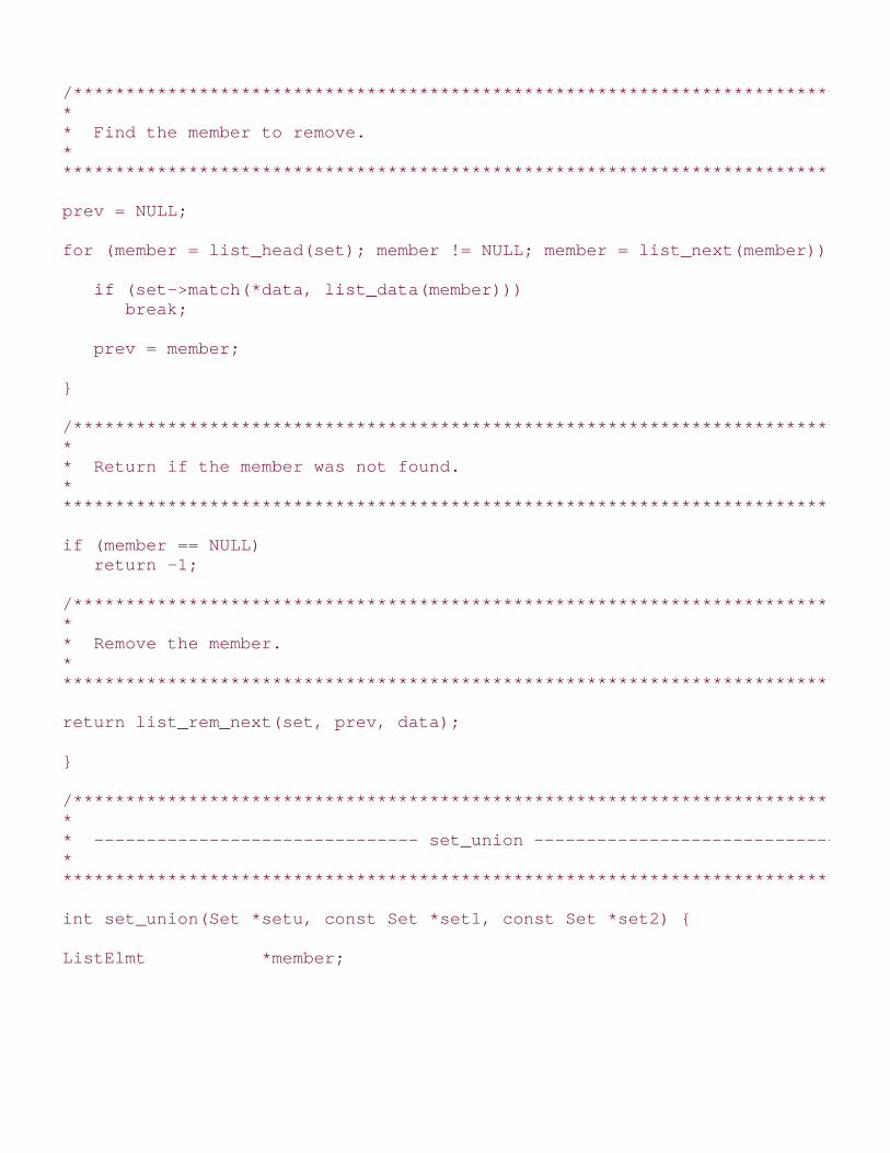
/****************************************************************************** ** Find the member to remove. ** ******************************************************************************/
prev = NULL;
for (member = list_head(set); member != NULL; member = list_next(member)) {
if (set->match(*data, list_data(member))) break;
prev = member;
}
/****************************************************************************** ** Return if the member was not found. ** ******************************************************************************/
if (member == NULL) return -1;
/****************************************************************************** ** Remove the member. ** ******************************************************************************/
return list_rem_next(set, prev, data);
}
/****************************************************************************** ** ------------------------------- set_union ------------------------------ ** ******************************************************************************/
int set_union(Set *setu, const Set *set1, const Set *set2) {
ListElmt *member;
void *data;
/****************************************************************************** ** Initialize the set for the union. ** ******************************************************************************/
set_init(setu, set1->match, NULL);
/****************************************************************************** ** Insert the members of the first set. ** ******************************************************************************/
for (member = list_head(set1); member != NULL; member = list_next(member)) {
data = list_data(member);
if (list_ins_next(setu, list_tail(setu), data) != 0) {
set_destroy(setu); return -1;
}
}
/****************************************************************************** ** Insert the members of the second set. ** ******************************************************************************/
for (member = list_head(set2); member != NULL; member = list_next(member)) {
if (set_is_member(set1, list_data(member))) {
/*********************************************************************** * * * Do not allow the insertion of duplicates. * * * ***********************************************************************/
continue;

}
else {
data = list_data(member);
if (list_ins_next(setu, list_tail(setu), data) != 0) {
set_destroy(setu); return -1;
}
}
}
return 0;
}
/****************************************************************************** ** --------------------------- set_intersection --------------------------- ** ******************************************************************************/
int set_intersection(Set *seti, const Set *set1, const Set *set2) {
ListElmt *member;
void *data;
/****************************************************************************** ** Initialize the set for the intersection. ** ******************************************************************************/
set_init(seti, set1->match, NULL);
/****************************************************************************** ** Insert the members present in both sets. ** ******************************************************************************/

for (member = list_head(set1); member != NULL; member = list_next(member)) {
if (set_is_member(set2, list_data(member))) {
data = list_data(member);
if (list_ins_next(seti, list_tail(seti), data) != 0) {
set_destroy(seti); return -1;
}
}
}
return 0;
}
/****************************************************************************** ** ---------------------------- set_difference ---------------------------- ** ******************************************************************************/
int set_difference(Set *setd, const Set *set1, const Set *set2) {
ListElmt *member;
void *data;
/****************************************************************************** ** Initialize the set for the difference. ** ******************************************************************************/
set_init(setd, set1->match, NULL);
/****************************************************************************** ** Insert the members from set1 not in set2. ** *

*****************************************************************************/
for (member = list_head(set1); member != NULL; member = list_next(member)) {
if (!set_is_member(set2, list_data(member))) {
data = list_data(member);
if (list_ins_next(setd, list_tail(setd), data) != 0) {
set_destroy(setd); return -1;
}
}
}
return 0;
}
/****************************************************************************** ** ----------------------------- set_is_member ---------------------------- ** ******************************************************************************/
int set_is_member(const Set *set, const void *data) {
ListElmt *member;
/****************************************************************************** ** Determine if the data is a member of the set. ** ******************************************************************************/
for (member = list_head(set); member != NULL; member = list_next(member)) {
if (set->match(data, list_data(member))) return 1;
}

return 0;
}
/****************************************************************************** ** ----------------------------- set_is_subset ---------------------------- ** ******************************************************************************/
int set_is_subset(const Set *set1, const Set *set2) {
ListElmt *member;
/****************************************************************************** ** Do a quick test to rule out some cases. ** ******************************************************************************/
if (set_size(set1) > set_size(set2)) return 0;
/****************************************************************************** ** Determine if set1 is a subset of set2. ** ******************************************************************************/
for (member = list_head(set1); member != NULL; member = list_next(member)) {
if (!set_is_member(set2, list_data(member))) return 0;
}
return 1;
}
/****************************************************************************** ** ------------------------------ set_is_equal ---------------------------- ** ******************************************************************************/

int set_is_equal(const Set *set1, const Set *set2) {
/****************************************************************************** ** Do a quick test to rule out some cases. ** ******************************************************************************/
if (set_size(set1) != set_size(set2)) return 0;
/****************************************************************************** ** Sets of the same size are equal if they are subsets. ** ******************************************************************************/
return set_is_subset(set1, set2);
}
Top

Mastering Algorithms with CBy Kyle LoudonSlots : 1Table of ContentsChapter 7. Sets
Content
7.4 Set Example: Set Covering
Set covering is an optimization problem that nicely models many problems of combinatorics and resourceselection . Here is the idea: given a set S and a set P of subsets A 1 to An of S , set C , which is composedof one or more sets from P , is said to cover S if each member in S is contained in at least one of thesubsets in C ; in addition, C contains as few sets from P as possible.
As an example, imagine trying to form a team from a large set of candidate players, each with a certain setof skills. The goal is to form the smallest team possible possessing a certain set of skills overall. That is, forany skill required by the team as a whole, at least one player on the team must possess the skill. Let S bethe skills that must be present on the team, and let P be the sets of skills possessed by various candidateplayers. The various player skill sets in P that are placed in set C together must cover all of the skills in setS . But remember, we must select as few players as possible.
The algorithm presented here for set covering is an approximation algorithm (see Chapter 1 ). It does notalways obtain the best solution, but it does come within a logarithmic bound. The algorithm works byrepeatedly picking a set from P that covers the most members not yet covered in S . In other words, it triesto cover as much of S as it can as early as it can. Thus, the algorithm is greedy (see Chapter 1 ). As eachset is selected from P , it is removed, and its members are removed from S as well. When there are nomembers left to cover in S , the cover set C is complete.
Let's look at finding the optimal covering of a set of twelve skills S = {a, b, c, d, e, f, g, h, i, j, k, l}considering a set of seven candidate players P = {A 1 , …, A 7 }. The players in P have the followingassortments of skills: A 1 = {a, b, c, d}, A 2 = {e, f, g, h, i}, A 3 = {j, k, l}, A 4 = {a, e}, A 5 = {b, f, g}, A
6 = {c, d, g, h, k, l}, and A 7 = {l}. The optimal covering is C = {A 1 , A 2 , A 3 }. The algorithm presentedhere selects the set C = {A 6 , A 2 , A 1 , A 3 } (see Figure 7.2 ).
Figure 7.2. A set covering problem

Examples Example 7.3 and Example 7.4 present a function, cover , that determines a nearly optimal
covering of S considering the subsets A 1 to An in P . The function has three arguments: members is the
set S to be covered, subsets is the set of subsets in P , and covering is the set C returned as the
covering. The function modifies all three sets passed to it, so copies should be made before calling thefunction, if necessary.
To begin, covering is initialized by calling set_init . The outermost loop iterates as long as there are
noncovered members in members and the algorithm has not run out of subsets for the covering. Inside
this loop, during each iteration, it finds the set in subsets that produces the largest intersection with
members . It then adds this set to the covering and removes its members from members . Last in the
loop, the selected set is removed from subsets . If the outermost loop terminates with members not
empty, then a complete covering was not possible using the sets in subsets . This is also the case if
during any iteration none of the sets in subsets intersects with members . The function cover returns
if it finds a covering, 1 if a covering is not possible, or -1 otherwise.
The runtime complexity of cover is O (m 3 ), where m is the initial number of members in members . This
occurs when there is exactly one subset in subsets for each member in members ; consequently,
there are m subsets. In this case, set-intersection runs in O (m ) time because each subset contains only
one member to traverse when computing the intersection with members . Thus, the inner loop of cover is
O (m 2 ) and this loop is executed m times.
Example 7.3. Header for Set Covering
/*****************************************************************************

* ** -------------------------------- cover.h ------------------------------- ** ******************************************************************************/
#ifndef COVER_H#define COVER_H
#include "set.h"
/****************************************************************************** ** Define a structure for subsets identified by a key. ** ******************************************************************************/
typedef struct KSet_ {
void *key;Set set;
} KSet;
/****************************************************************************** ** --------------------------- Public Interface --------------------------- ** ******************************************************************************/
int cover(Set *members, Set *subsets, Set *covering);
#endif
Example 7.4. Implementation of a Function for Set Covering
/****************************************************************************** ** -------------------------------- cover.c ------------------------------- ** ******************************************************************************/
#include <stdlib.h>
#include "cover.h"#include "list.h"#include "set.h"
/****************************************************************************** ** --------------------------------- cover -------------------------------- ** ******************************************************************************/
int cover(Set *members, Set *subsets, Set *covering) {
Set intersection;
KSet *subset;
ListElmt *member, *max_member;
void *data;
int max_size;
/****************************************************************************** ** Initialize the covering. ** ******************************************************************************/
set_init(covering, subsets->match, NULL);
/****************************************************************************** ** Continue while there are noncovered members and candidate subsets. ** ******************************************************************************/
while (set_size(members) > 0 && set_size(subsets) > 0) {
/************************************************************************** * * * Find the subset that covers the most members. * * * **************************************************************************/
max_size = 0;
for (member = list_head(subsets); member != NULL; member = list_next(member)) {

if (set_intersection(&intersection, &((KSet *)list_data(member))->set, members) != 0) {
return -1;
}
if (set_size(&intersection) > max_size) {
max_member = member; max_size = set_size(&intersection);
}
set_destroy(&intersection);
}
/************************************************************************** * * * A covering is not possible if there was no intersection. * * * **************************************************************************/
if (max_size == 0) return 1;
/************************************************************************** * * * Insert the selected subset into the covering. * * * **************************************************************************/
subset = (KSet *)list_data(max_member);
if (set_insert(covering, subset) != 0) return -1;
/************************************************************************** * * * Remove each covered member from the set of noncovered members. * * * **************************************************************************/
for (member = list_head(&((KSet *)list_data(max_member))->set); member != NULL; member = list_next(member)) {

data = list_data(member);
if (set_remove(members, (void**)&data) == 0 && members->destroy != NULL) members->destroy(data);
}
/************************************************************************** * * * Remove the subset from the set of candidate subsets. * * * **************************************************************************/
if (set_remove(subsets, (void **)&subset) != 0) return -1;
}
/****************************************************************************** ** No covering is possible if there are still noncovered members. ** ******************************************************************************/
if (set_size(members) > 0) return -1;
return 0;
}
Top

Mastering Algorithms with CBy Kyle Loudon
Slots : 1
Table of Contents
Chapter 7. Sets
Content
7.5 Questions and Answers
Q: Instead of implementing set_is_subset as shown, how could we use other set operations todetermine if one set, S1, is a subset of another set, S2? Why is set_is_subset provided?
A: In set notation, if S1 S2 = S1, then S1 S2. Therefore, we could use a combination of theset_intersection and set_is_equal operations. Whether we implement this operation as shown or useset_intersection and set_is_equal, its runtime complexity is O (mn), where m is the size of S1 and nis the size of S2. However, in the case of calling set_intersection and set_is_equal, the running timeis actually closer to T (m, n) = 2mn because both set_intersection and set_is_equal run in T (m, n)= mn times some constant. Compare this with the operation set_is_subset, which runs closer to T(m, n) = mn. Although the complexities of the two methods are the same, calling set_intersectionand set_is_equal requires approximately double the time in practice.
Q: Instead of implementing set_is_equal as shown, how could we use other set operations todetermine if one set, S1, is equal to another set, S2?
A: In set notation, if S1 - S2 = and S2 - S1 = , then S1 = S2. Therefore, we could implementthis, albeit less efficiently, using two calls to set_difference and two calls to set_size.
Q: Instead of implementing set_intersection as shown, how could we use the set_differenceoperation to compute the intersection of two sets, S1 and S2?
A: In set notation, S1 S2 = S1 - (S1 - S2). Therefore, we could implement this, albeit lessefficiently, using two calls to set_difference.
Q: Why was list_ins_next used instead of set_insert to insert members into the sets built withinset_union, set_intersection, and set_difference?
A: Recall that the running time of set_insert is O (n) because it traverses a set to ensure that themember being inserted is not duplicated. Since the set_union, set_intersection, and set_differenceoperations ensure this already, it is considerably more efficient to call the O (1) operationlist_ins_next instead.
Q: Suppose we have three sets, S1 = {1, 2, 3 }, S2 = {1, 4, 5}, and S3 = {1}. What is the result of
the set operations S1 S2 , S1 - (S2 S3) , and (S1 S2) - S3?

A: S1 S2 = {1, 2, 3, 4, 5}, S1 - (S2 S3) = {2, 3}, and (S1 S2) - S3 = .
Q: Using the properties and basic operations presented for sets, simplify (((S1 S2) (S1 S3)) -
(S1 (S2 S3))) (S1 S2).
Applying the distributive law produces:
Applying set difference produces:
Applying the empty set law produces:
Q: The symmetric difference of two sets consists of those members that are in either of the two sets,but not both. The notation for the symmetric difference of two sets, S1 and S2, is S1 D S2. How couldwe implement a symmetric difference operation using the set operations presented in this chapter?Could this operation be implemented more efficiently some other way?
A: In set notation, S1 D S2 = (S1 - S2) (S2 - S1). Therefore, we could implement this operationusing two calls to set_difference followed by a call to set_union. This produces a worst-case runningtime of T (m, n) = 3mn times some constant, for a complexity of O (mn), where m is the size of S1
and n is the size of S2. For example, consider the sets S1 = {1, 2, 3} and S2 = {4, 5, 6}, whichrepresent a worst-case scenario. To compute S1 - S2, we must search all of S2 for each member inS1, which results in the set {1, 2, 3}. Similarly, to compute S2 - S1, we must search all of S1 for eachmember of S2, which results in the set {4, 5, 6}. Since both sets are the same size as the originalsets, sizes m and n, their union is another operation that runs in time proportionate to m times n.However, since we know that the sets produced by S1 - S2 and S2 - S1 will not generate anyduplicate members between them, we could avoid the use of set_union and simply insert eachmember into the final set by calling the O (1) operation list_ins_next once for each member m + ntimes. This is a better implementation in practice, but it does not change the overall complexity.
Q: A multiset (see the related topics at the end of the chapter) is a type of set that allows membersto occur more than once. How would the runtime complexities of inserting and removing memberswith a multiset compare with the operations for inserting and removing members in this chapter?
A: When inserting a member into a set, in which members may not be duplicated, we must searchthe entire set to ensure that we do not duplicate a member. This is an O (n) process. Removing amember from a set is O (n) as well because we may have to search the entire set again. In amultiset, inserting a member is considerably more efficient because we do not have to traverse themembers looking for duplicates. Therefore, we can insert the new member in O (1) time. In amultiset, removing a member remains an O (n) process because we still must search for the memberwe want to remove.

Top

Mastering Algorithms with CBy Kyle Loudon
Slots : 1
Table of Contents
Chapter 7. Sets
Content
7.6 Related Topics
Venn diagrams
Graphical representations of sets that help determine the results of set operations visually. Forexample, a Venn diagram depicting two intersecting sets consists of two slightly overlappingcircles. The overlapping regions represent the intersection of the sets.
Bit-vector representation
A representation for sets useful when the universe is small and known. Each member in theuniverse is represented as a bit in an array. If a member exists in the set, its bit is set to 1;otherwise, its bit is set to 0.
Multisets
Sets in which members may be duplicated. In some problems the restriction of no duplicatemembers is too strict. A multiset is an alternative type of set for these problems.
Top

Mastering Algorithms with CBy Kyle Loudon
Slots : 1
Table of Contents
Part II: Data Structures
Content
Chapter 8. Hash TablesHash tables support one of the most efficient types of searching: hashing. Fundamentally, a hashtable consists of an array in which data is accessed via a special index called a key. The primary ideabehind a hash table is to establish a mapping between the set of all possible keys and positions in thearray using a hash function. A hash function accepts a key and returns its hash coding, or hashvalue. Keys vary in type, but hash codings are always integers.
Since both computing a hash value and indexing into an array can be performed in constant time, thebeauty of hashing is that we can use it to perform constant-time searches. When a hash function canguarantee that no two keys will generate the same hash coding, the resulting hash table is said to bedirectly addressed. This is ideal, but direct addressing is rarely possible in practice. For example,imagine a phone-mail system in which eight-character names are hashed to find messages for usersin the system. If we were to rely on direct addressing, the hash table would contain more than 268 =(2.09)1011 entries, and the majority would be unused since most character combinations are notnames.
Typically, the number of entries in a hash table is small relative to the universe of possible keys.Consequently, most hash functions map some keys to the same position in the table. When two keysmap to the same position, they collide. A good hash function minimizes collisions, but we must stillbe prepared to deal with them. This chapter presents two types of hash tables that resolve collisionsin different ways.
This chapter covers:
Chained hash tables
Hash tables that store data in buckets. Each bucket is a linked list that can grow as large asnecessary to accommodate collisions.
Open-addressed hash tables
Hash tables that store data in the table itself instead of in buckets. Collisions are resolved usingvarious methods of probing the table.
Selecting a hash function
The crux of hashing. By distributing keys in a random manner about the table, collisions areminimized. Thus, it is important to select a hash function that accomplishes this.
Collision resolution

Methods of managing when several keys map to the same index. Chained hash tables have aninherent way to resolve collisions. Open-addressed hash tables use various forms of probing.
Some applications of hash tables are:
Database systems
Specifically, those that require efficient random access. Generally, database systems try tooptimize between two types of access methods: sequential and random. Hash tables are animportant part of efficient random access because they provide a way to locate data in aconstant amount of time.
Symbol tables (illustrated in this chapter)
The tables used by compilers to maintain information about symbols from a program.Compilers access information about symbols frequently. Therefore, it is important that symboltables be implemented very efficiently.
Tagged buffers
A mechanism for storing and retrieving data in a machine-independent manner. Each datamember resides at a fixed offset in the buffer. A hash table is stored in the buffer so that thelocation of each tagged member can be ascertained quickly. One use of a tagged buffer issending structured data across a network to a machine whose byte ordering and structurealignment may not be the same as the original host's. The buffer handles these concerns asthe data is stored and extracted member by member.
Data dictionaries
Data structures that support adding, deleting, and searching for data. Although the operationsof a hash table and a data dictionary are similar, other data structures may be used toimplement data dictionaries. Using a hash table is particularly efficient.
Associative arrays
Most commonly used in languages that do not support structured types. Associative arraysconsist of data arranged so that the n th element of one array corresponds to the n th elementof another. Associative arrays are useful for indexing a logical grouping of data by several keyfields. A hash table helps to key into each array efficiently.
Top

Mastering Algorithms with CBy Kyle LoudonSlots : 1Table of ContentsChapter 8. Hash Tables
Content
8.1 Description of Chained Hash Tables
A chained hash table fundamentally consists of an array of linked lists . Each list forms a bucket in which weplace all elements hashing to a specific position in the array (see Figure 8.1 ). To insert an element, we firstpass its key to a hash function in a process called hashing the key . This tells us in which bucket theelement belongs. We then insert the element at the head of the appropriate list. To look up or remove anelement, we hash its key again to find its bucket, then traverse the appropriate list until we find theelement we are looking for. Because each bucket is a linked list, a chained hash table is not limited to afixed number of elements. However, performance degrades if the table becomes too full.
Figure 8.1. A chained hash table with five buckets containing a total of sevenelements
8.1.1 Collision Resolution
When two keys hash to the same position in a hash table, they collide . Chained hash tables have a simplesolution for resolving collisions: elements are simply placed in the bucket where the collision occurs. One

problem with this, however, is that if an excessive number of collisions occur at a specific position, a bucketbecomes longer and longer. Thus, accessing its elements takes more and more time.
Ideally, we would like all buckets to grow at the same rate so that they remain nearly the same size and assmall as possible. In other words, the goal is to distribute elements about the table in as uniform andrandom a manner as possible. This theoretically perfect situation is known as uniform hashing ; however, inpractice it usually can only be approximated.
Even assuming uniform hashing, performance degrades significantly if we make the number of buckets inthe table small relative to the number of elements we plan to insert. In this situation, all of the bucketsbecome longer and longer. Thus, it is important to pay close attention to a hash table's load factor . Theload factor of a hash table is defined as:
where n is the number of elements in the table and m is the number of positions into which elements maybe hashed. The load factor of a chained hash table indicates the maximum number of elements we canexpect to encounter in a bucket, assuming uniform hashing.
For example, in a chained hash table with m = 1699 buckets and a total of n = 3198 elements, the loadfactor of the table is a = 3198/1699 = 2. Therefore, in this case, we can expect to encounter no more thantwo elements while searching any one bucket. When the load factor of a table drops below 1, each positionwill probably contain no more than one element. Of course, since uniform hashing is only approximated, inactuality we end up encountering somewhat more or less than what the load factor suggests. How close wecome to uniform hashing ultimately depends on how well we select our hash function.
8.1.2 Selecting a Hash Function
The goal of a good hash function is to approximate uniform hashing, that is, to spread elements about ahash table in as uniform and random a manner as possible. A hash function h is a function we define tomap a key k to some position x in a hash table. x is called the hash coding of k . Formally stated:
h(k) = x
Generally, most hashing methods assume k to be an integer so that it may be easily altered mathematicallyto make h distribute elements throughout the table more uniformly. When k is not an integer, we canusually coerce it into one without much difficulty.
Precisely how to coerce a set of keys depends a great deal on the characteristics of the keys themselves.Therefore, it is important to gain as much of a qualitative understanding of them in a particular applicationas we can. For example, if we were to hash the identifiers found in a program, we might observe that many
have similar prefixes and suffixes since developers tend to gravitate toward variables such as sampleptr, simpleptr , and sentryptr . A poor way to coerce these keys would be any method depending
strictly on characters at the beginning and end of the keys, since this would result in many of the sameintegers for k . On the other hand, we might try selecting characters from four positions that have thepropensity to be somewhat random, permute them in a way that randomizes them further, and stuff theminto specific bytes of a four-byte integer. Whatever approach we choose for coercing keys, the mostimportant thing to remember, again, is that a hash function should distribute a set of keys about a hashtable in a uniform and random manner.
8.1.2.1 Division method
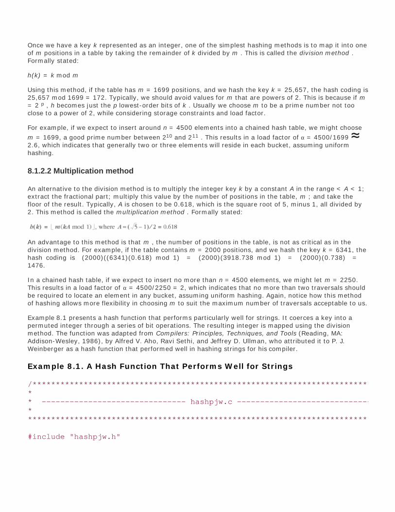
Once we have a key k represented as an integer, one of the simplest hashing methods is to map it into oneof m positions in a table by taking the remainder of k divided by m . This is called the division method .Formally stated:
h(k) = k mod m
Using this method, if the table has m = 1699 positions, and we hash the key k = 25,657, the hash coding is25,657 mod 1699 = 172. Typically, we should avoid values for m that are powers of 2. This is because if m= 2 p , h becomes just the p lowest-order bits of k . Usually we choose m to be a prime number not tooclose to a power of 2, while considering storage constraints and load factor.
For example, if we expect to insert around n = 4500 elements into a chained hash table, we might choose
m = 1699, a good prime number between 210 and 211 . This results in a load factor of a = 4500/1699 2.6, which indicates that generally two or three elements will reside in each bucket, assuming uniformhashing.
8.1.2.2 Multiplication method
An alternative to the division method is to multiply the integer key k by a constant A in the range < A < 1;extract the fractional part; multiply this value by the number of positions in the table, m ; and take thefloor of the result. Typically, A is chosen to be 0.618, which is the square root of 5, minus 1, all divided by2. This method is called the multiplication method . Formally stated:
An advantage to this method is that m , the number of positions in the table, is not as critical as in thedivision method. For example, if the table contains m = 2000 positions, and we hash the key k = 6341, thehash coding is (2000)((6341)(0.618) mod 1) = (2000)(3918.738 mod 1) = (2000)(0.738) =1476.
In a chained hash table, if we expect to insert no more than n = 4500 elements, we might let m = 2250.This results in a load factor of a = 4500/2250 = 2, which indicates that no more than two traversals shouldbe required to locate an element in any bucket, assuming uniform hashing. Again, notice how this methodof hashing allows more flexibility in choosing m to suit the maximum number of traversals acceptable to us.
Example 8.1 presents a hash function that performs particularly well for strings. It coerces a key into apermuted integer through a series of bit operations. The resulting integer is mapped using the divisionmethod. The function was adapted from Compilers: Principles, Techniques, and Tools (Reading, MA:Addison-Wesley, 1986), by Alfred V. Aho, Ravi Sethi, and Jeffrey D. Ullman, who attributed it to P. J.Weinberger as a hash function that performed well in hashing strings for his compiler.
Example 8.1. A Hash Function That Performs Well for Strings
/****************************************************************************** ** ------------------------------- hashpjw.c ------------------------------ ** ******************************************************************************/
#include "hashpjw.h"

/****************************************************************************** ** -------------------------------- hashpjw ------------------------------- ** ******************************************************************************/
int hashpjw(const void *key) {
const char *ptr;
int val;
/****************************************************************************** ** Hash the key by performing a number of bit operations on it. ** ******************************************************************************/
val = 0;ptr = key;
while (*ptr != '\0') {
int tmp;
val = (val << 4) + (*ptr);
if (tmp = (val & 0xf0000000)) {
val = val ^ (tmp >> 24); val = val ^ tmp;
}
ptr++;
}
/****************************************************************************** ** In practice, replace PRIME_TBLSIZ with the actual table size. ** ******************************************************************************/
return val % PRIME_TBLSIZ

;
}
Top

Mastering Algorithms with CBy Kyle Loudon
Slots : 1
Table of Contents
Chapter 8. Hash Tables
Content
8.2 Interface for Chained Hash Tables
chtbl_init
int chtbl_init(CHTbl *htbl, int buckets, int (*h)(const void *key), int (*match)(const void *key1, const void *key2), void (*destroy)(void *data));
Return Value
0if initializing the hash table is successful, or -1 otherwise.
Description
Initializes the chained hash table specified by htbl. This operation must be called for a chained hashtable before the hash table can be used with any other operation. The number of buckets allocated inthe hash table is specified by buckets. The function pointer h specifies a user-defined hash functionfor hashing keys. The function pointer match specifies a user-defined function to determine whethertwo keys match. It should return 1 if key1 is equal to key2, and otherwise. The destroyargument provides a way to free dynamically allocated data when chtbl_destroy is called. Forexample, if the hash table contains data dynamically allocated using malloc, destroy should be setto free to free the data as the hash table is destroyed. For structured data containing severaldynamically allocated members, destroy should be set to a user-defined function that calls free foreach dynamically allocated member as well as for the structure itself. For a hash table containing datathat should not be freed, destroy should be set to NULL.
Complexity
O (m), where m is the number of buckets in the hash table.
chtbl_destroy

void chtbl_destroy(CHTbl *htbl);
Return Value
None.
Description
Destroys the chained hash table specified by htbl. No other operations are permitted after callingchtbl_destroy unless chtbl_init is called again. The chtbl_destroy operation removes all elements froma hash table and calls the function passed as destroy to chtbl_init once for each element as it isremoved, provided destroy was not set to NULL.
Complexity
O (m), where m is the number of buckets in the hash table.
chtbl_insert
int chtbl_insert(CHTbl *htbl, const void *data);
Return Value
0if inserting the element is successful, 1 if the element is already in the hash table, or -1 otherwise.
Description
Inserts an element into the chained hash table specified by htbl. The new element contains apointer to data, so the memory referenced by data should remain valid as long as the elementremains in the hash table. It is the responsibility of the caller to manage the storage associated withdata.
Complexity
O (1)
chtbl_remove
int chtbl_remove(CHTbl *htbl, void **data);

Return Value
0if removing the element is successful, or -1 otherwise.
Description
Removes the element matching data from the chained hash table specified by htbl. Upon return,data points to the data stored in the element that was removed. It is the responsibility of the callerto manage the storage associated with the data.
Complexity
O (1)
chtbl_lookup
int chtbl_lookup(const CHTbl *htbl, void **data);
Return Value
0if the element is found in the hash table, or -1 otherwise.
Description
Determines whether an element matches data in the chained hash table specified by htbl. If amatch is found, data points to the matching data in the hash table upon return.
Complexity
O (1)
chtbl_size
int chtbl_size(CHTbl *htbl);
Return Value
Number of elements in the hash table.
Description

Macro that evaluates to the number of elements in the chained hash table specified by htbl.
Complexity
O (1)
Top
Mastering Algorithms with CBy Kyle LoudonSlots : 1Table of ContentsChapter 8. Hash Tables
Content
8.3 Implementation and Analysis of Chained Hash Tables
A chained hash table consists of an array of buckets. Each bucket is a linked list containing the elements
that hash to a certain position in the table. The structure CHTbl is the chained hash table data structure
(see Example 8.2 ). This structure consists of six members: buckets is the number of buckets allocated
in the table; h , match , and destroy are members used to encapsulate the functions passed to
chtbl_init ; size is the number of elements currently in the table; and table is the array of buckets.
Example 8.2. Header for the Chained Hash Table Abstract Datatype
/****************************************************************************** ** ------------------------------- chtbl.h -------------------------------- ** ******************************************************************************/
#ifndef CHTBL_H#define CHTBL_H
#include <stdlib.h>
#include "list.h"
/****************************************************************************** ** Define a structure for chained hash tables. ** ******************************************************************************/

typedef struct CHTbl_ {
int buckets;
int (*h)(const void *key);int (*match)(const void *key1, const void *key2);void (*destroy)(void *data);
int size;List *table;
} CHTbl;
/****************************************************************************** ** --------------------------- Public Interface --------------------------- ** ******************************************************************************/
int chtbl_init(CHTbl *htbl, int buckets, int (*h)(const void *key), int (*match)(const void *key1, const void *key2), void (*destroy)(void *data));
void chtbl_destroy(CHTbl *htbl);
int chtbl_insert(CHTbl *htbl, const void *data);
int chtbl_remove(CHTbl *htbl, void **data);
int chtbl_lookup(const CHTbl *htbl, void **data);
#define chtbl_size(htbl) ((htbl)->size)
#endif
8.3.1 chtbl_init
The chtbl_init operation initializes a chained hash table so that it can be used in other operations (seeExample 8.3 ). Initializing a chained hash table is a simple operation in which we allocate space for the
buckets; initialize each bucket by calling list_init ; encapsulate the h , match , and destroy functions;
and set the size member to 0.
The runtime complexity of chtbl_init is O (m ), where m is the number of buckets in the table. This isbecause the O (1) operation list_init must be called once for each of the m buckets. All other parts of theoperation run in a constant amount of time.
8.3.2 chtbl_destroy

The chtbl_destroy operation destroys a chained hash table (see Example 8.3 ). Primarily this meansremoving the elements from each bucket and freeing the memory chtbl_init allocated for the table. The
function passed as destroy to chtbl_init is called once for each element as it is removed, provided
destroy was not set to NULL.
The runtime complexity of chtbl_destroy is O (m ), where m is the number of buckets in the table. This isbecause list_destroy is called once for each bucket. In each bucket, we expect to remove a number ofelements equal to the load factor of the hash table, which is treated as a small constant.
8.3.3 chtbl_insert
The chtbl_insert operation inserts an element into a chained hash table (see Example 8.3 ). Since a key isnot allowed to be inserted into the hash table more than once, chtbl_lookup is called to make sure that thetable does not already contain the new element. If no element with the same key already exists in the hashtable, we hash the key for the new element and insert it into the bucket at the position in the hash tablethat corresponds to the hash coding. If this is successful, we increment the table size.
Assuming we approximate uniform hashing well, the runtime complexity of chtbl_insert is O (1), sincechtbl_lookup , hashing a key, and inserting an element at the head of a linked list all run in a constantamount of time.
8.3.4 chtbl_remove
The chtbl_remove operation removes an element from a chained hash table (see Example 8.3 ). To removethe element, we hash its key, search the appropriate bucket for an element with a key that matches, and
call list_rem_next to remove it. The pointer prev maintains a pointer to the element before the one to be
removed since list_rem_next requires this. Recall that list_rem_next sets data to point to the data
removed from the table. If a matching key is not found in the bucket, the element is not in the table. Ifremoving the element is successful, we decrease the table size by 1.
Assuming we approximate uniform hashing well, the runtime complexity of chtbl_remove is O (1). This isbecause we expect to search a number of elements equal to the load factor of the hash table, which istreated as a small constant.
8.3.5 chtbl_lookup
The chtbl_lookup operation searches for an element in a chained hash table and returns a pointer to it (seeExample 8.3 ). This operation works much like chtbl_remove , except that once the element is found, it isnot removed from the table.
Assuming we approximate uniform hashing well, the runtime complexity of chtbl_lookup is O (1). This isbecause we expect to search a number of elements equal to the load factor of the hash table, which istreated as a small constant.
8.3.6 chtbl_size
This macro evaluates to the number of elements in a chained hash table (see Example 8.2 ). It works by
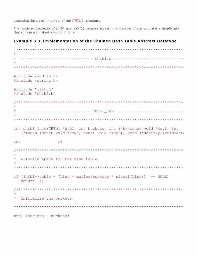
accessing the size member of the CHTbl structure.
The runtime complexity of chtbl_size is O (1) because accessing a member of a structure is a simple taskthat runs in a constant amount of time.
Example 8.3. Implementation of the Chained Hash Table Abstract Datatype
/****************************************************************************** ** ------------------------------- chtbl.c -------------------------------- ** ******************************************************************************/
#include <stdlib.h>#include <string.h>
#include "list.h"#include "chtbl.h"
/****************************************************************************** ** ------------------------------ chtbl_init ------------------------------ ** ******************************************************************************/
int chtbl_init(CHTbl *htbl, int buckets, int (*h)(const void *key), int (*match)(const void *key1, const void *key2), void (*destroy)(void*data)) {
int i;
/****************************************************************************** ** Allocate space for the hash table. ** ******************************************************************************/
if ((htbl->table = (List *)malloc(buckets * sizeof(List))) == NULL) return -1;
/****************************************************************************** ** Initialize the buckets. ** ******************************************************************************/
htbl->buckets = buckets;

for (i = 0; i < htbl->buckets; i++) list_init(&htbl->table[i], destroy);
/****************************************************************************** ** Encapsulate the functions. ** ******************************************************************************/
htbl->h = h;htbl->match = match;htbl->destroy = destroy;
/****************************************************************************** ** Initialize the number of elements in the table. ** ******************************************************************************/
htbl->size = 0;
return 0;
}
/****************************************************************************** ** ---------------------------- chtbl_destroy ----------------------------- ** ******************************************************************************/
void chtbl_destroy(CHTbl *htbl) {
int i; /****************************************************************************** ** Destroy each bucket. ** ******************************************************************************/
for (i = 0; i < htbl->buckets; i++) {
list_destroy(&htbl->table[i]);
}
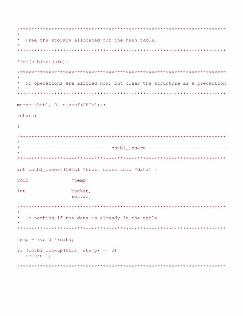
/****************************************************************************** ** Free the storage allocated for the hash table. ** ******************************************************************************/
free(htbl->table);
/****************************************************************************** ** No operations are allowed now, but clear the structure as a precaution. ** ******************************************************************************/
memset(htbl, 0, sizeof(CHTbl));
return;
}
/****************************************************************************** ** ----------------------------- chtbl_insert ----------------------------- ** ******************************************************************************/
int chtbl_insert(CHTbl *htbl, const void *data) {
void *temp;
int bucket, retval; /****************************************************************************** ** Do nothing if the data is already in the table. ** ******************************************************************************/
temp = (void *)data;
if (chtbl_lookup(htbl, &temp) == 0) return 1;
/*****************************************************************************

* ** Hash the key. ** ******************************************************************************/
bucket = htbl->h(data) % htbl->buckets;
/****************************************************************************** ** Insert the data into the bucket. ** ******************************************************************************/
if ((retval = list_ins_next(&htbl->table[bucket], NULL, data)) == 0) htbl->size++;
return retval;
}
/****************************************************************************** ** ----------------------------- chtbl_remove ----------------------------- ** ******************************************************************************/
int chtbl_remove(CHTbl *htbl, void **data) {
ListElmt *element, *prev;
int bucket; /****************************************************************************** ** Hash the key. ** ******************************************************************************/
bucket = htbl->h(*data) % htbl->buckets;
/****************************************************************************** ** Search for the data in the bucket. ** ******************************************************************************/

prev = NULL;
for (element = list_head(&htbl->table[bucket]); element != NULL; element = list_next(element)) {
if (htbl->match(*data, list_data(element))) {
/*********************************************************************** * * * Remove the data from the bucket. * * * ***********************************************************************/
if (list_rem_next(&htbl->table[bucket], prev, data) == 0) {
htbl->size--; return 0;
}
else {
return -1;
}
}
prev = element;
}
/****************************************************************************** ** Return that the data was not found. ** ******************************************************************************/
return -1;
}
/****************************************************************************** ** ----------------------------- chtbl_lookup ----------------------------- ** *

*****************************************************************************/
int chtbl_lookup(const CHTbl *htbl, void **data) {
ListElmt *element;
int bucket; /****************************************************************************** ** Hash the key. ** ******************************************************************************/
bucket = htbl->h(*data) % htbl->buckets;
/****************************************************************************** ** Search for the data in the bucket. ** ******************************************************************************/
for (element = list_head(&htbl->table[bucket]); element != NULL; element = list_next(element)) {
if (htbl->match(*data, list_data(element))) {
/*********************************************************************** * * * Pass back the data from the table. * * * ***********************************************************************/
*data = list_data(element); return 0;
}
}
/****************************************************************************** ** Return that the data was not found. ** ******************************************************************************/
return -1;
}
Top

Mastering Algorithms with CBy Kyle LoudonSlots : 1Table of ContentsChapter 8. Hash Tables
Content
8.4 Chained Hash Table Example: Symbol Tables
An important application of hash tables is the way compilers maintain information about symbolsencountered in a program. Formally, a compiler translates a program written in one language, a sourcelanguage such as C, into another language, which is a set of instructions for the machine on which theprogram will run. In order to maintain information about the symbols in a program, compilers make use ofa data structure called a symbol table . Symbol tables are often implemented as hash tables because acompiler must be able to store and retrieve information about symbols very quickly.
Several parts of a compiler access the symbol table during various phases of the compilation process. Onepart, the lexical analyzer , inserts symbols. The lexical analyzer is the part of a compiler charged withgrouping characters from the source code into meaningful strings, called lexemes. These are translated intosyntactic elements, called tokens , that are passed on to the parser . The parser performs syntacticalanalysis. As the lexical analyzer encounters symbols in its input stream, it stores information about theminto the symbol table. Two important attributes stored by the lexical analyzer are a symbol's lexeme andthe type of token the lexeme constitutes (e.g., an identifier or an operator).
The example presented here is a very simple lexical analyzer that analyzes a string of characters and thengroups the characters into one of two types of tokens: a token consisting only of digits or a token consistingof something other than digits alone. For simplicity, we assume that tokens are separated in the inputstream by a single blank. The lexical analyzer is implemented as a function, lex (see Examples Example 8.4and Example 8.5 ), which a parser calls each time it requires another token.
The function works by first calling the next_token function (whose implementation is not shown) to get the
next blank-delimited string from the input stream istream . If next_token returns NULL, there are no
more tokens in the input stream. In this case, the function returns lexit , which tells the parser that
there are no more tokens to be processed. If next_token finds a string, some simple analysis is performedto determine what type of token the string represents. Next, the function inserts the lexeme and token type
together as a Symbol structure into the symbol table, symtbl , and returns the token type to the
parser. The type Symbol is defined in symbol.h , which is not included in this example.
A chained hash table is a good way to implement a symbol table because, in addition to being an efficientway to store and retrieve information, we can use it to store a virtually unlimited amount of data. This is

important for a compiler since it is difficult to know how many symbols a program will contain before lexicalanalysis.
The runtime complexity of lex is O (1), assuming next_token runs in a constant amount of time. This isbecause lex simply calls chtbl_insert , which is an O (1) operation.
Example 8.4. Header for a Simple Lexical Analyzer
/****************************************************************************** ** --------------------------------- lex.h -------------------------------- ** ******************************************************************************/
#ifndef LEX_H#define LEX_H
#include "chtbl.h"
/****************************************************************************** ** Define the token types recognized by the lexical analyzer. ** ******************************************************************************/
typedef enum Token_ {lexit, error, digit, other} Token;
/****************************************************************************** ** --------------------------- Public Interface --------------------------- ** ******************************************************************************/
Token lex(const char *istream, CHTbl *symtbl);
#endif
Example 8.5. Implementation of a Simple Lexical Analyzer
/****************************************************************************** ** --------------------------------- lex.c -------------------------------- ** ******************************************************************************/
#include <ctype.h>

#include <stdlib.h>#include <string.h>
#include "chtbl.h"#include "lex.h"#include "symbol.h"
/****************************************************************************** ** ---------------------------------- lex --------------------------------- ** ******************************************************************************/
Token lex(const char *istream, CHTbl *symtbl) {
Token token;
Symbol *symbol;
int length, retval, i;
/****************************************************************************** ** Allocate space for a symbol. ** ******************************************************************************/
if ((symbol = (Symbol *)malloc(sizeof(Symbol))) == NULL) return error;
/****************************************************************************** ** Process the next token. ** ******************************************************************************/
if ((symbol->lexeme = next_token(istream)) == NULL) {
/************************************************************************** * * * Return that there is no more input. * * * **************************************************************************/

free(symbol); return lexit;
}
else {
/************************************************************************** * * * Determine the token type. * * * **************************************************************************/
symbol->token = digit; length = strlen(symbol->lexeme);
for (i = 0; i < length; i++) {
if (!isdigit(symbol->lexeme[i])) symbol->token = other;
}
memcpy(&token, &symbol->token, sizeof(Token));
/************************************************************************** * * * Insert the symbol into the symbol table. * * * **************************************************************************/
if ((retval = chtbl_insert(symtbl, symbol)) < 0) {
free(symbol); return error;
}
else if (retval == 1) {
/*********************************************************************** * * * The symbol is already in the symbol table. * * * ***********************************************************************/
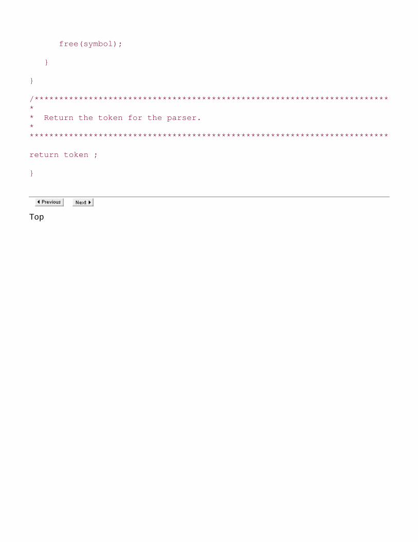
free(symbol);
}
}
/****************************************************************************** ** Return the token for the parser. ** ******************************************************************************/
return token ;
}
Top

Mastering Algorithms with CBy Kyle Loudon
Slots : 1
Table of Contents
Chapter 8. Hash Tables
Content
8.5 Description of Open-Addressed Hash Tables
In a chained hash table, elements reside in buckets extending from each position. In an open-addressed hash table, on the other hand, all elements reside in the table itself. This may beimportant for some applications that rely on the table being a fixed size. Without a way to extend thenumber of elements at each position, however, an open-addressed hash table needs another way toresolve collisions.
8.5.1 Collision Resolution
Whereas chained hash tables have an inherent means of resolving collisions, open-addressed hashtables must handle them in a different way. The way to resolve collisions in an open-addressed hashtable is to probe the table. To insert an element, for example, we probe positions until we find anunoccupied one, and insert the element there. To remove or look up an element, we probe positionsuntil the element is located or until we encounter an unoccupied position. If we encounter anunoccupied position before finding the element, or if we end up traversing all of the positions, theelement is not in the table.
Of course, the goal is to minimize how many probes we have to perform. Exactly how many positionswe end up probing depends primarily on two things: the load factor of the hash table and the degreeto which elements are distributed uniformly. Recall that the load factor of a hash table is a = n/m,where n is the number of elements and m is the number of positions into which the elements may behashed. Notice that since an open-addressed hash table cannot contain more elements than thenumber of positions in the table (n > m), its load factor is always less than or equal to 1. This makessense, since no position can ever contain more than one element.
Assuming uniform hashing, the number of positions we can expect to probe in an open-addressedhash table is:
For an open-addressed hash table that is half full (whose load factor is 0.5), for example, the numberof positions we can expect to probe is 1/(1 - 0.5) = 2. Table 8.1 illustrates how dramatically theexpected number of probes increases as the load factor of an open-addressed hash table approaches1 (or 100%), at which point the table is completely full. In a particularly time-sensitive application, itmay be advantageous to increase the size of the hash table to allow extra space for probing.
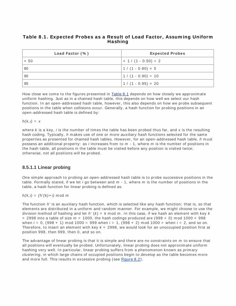
Table 8.1. Expected Probes as a Result of Load Factor, Assuming UniformHashing
Load Factor (%) Expected Probes
< 50 < 1 / (1 - 0.50) = 2
80 1 / (1 - 0.80) = 5
90 1 / (1 - 0.90) = 10
95 1 / (1 - 0.95) = 20
How close we come to the figures presented in Table 8.1 depends on how closely we approximateuniform hashing. Just as in a chained hash table, this depends on how well we select our hashfunction. In an open-addressed hash table, however, this also depends on how we probe subsequentpositions in the table when collisions occur. Generally, a hash function for probing positions in anopen-addressed hash table is defined by:
h(k,i) = x
where k is a key, i is the number of times the table has been probed thus far, and x is the resultinghash coding. Typically, h makes use of one or more auxiliary hash functions selected for the sameproperties as presented for chained hash tables. However, for an open-addressed hash table, h mustpossess an additional property: as i increases from to m - 1, where m is the number of positions inthe hash table, all positions in the table must be visited before any position is visited twice;otherwise, not all positions will be probed.
8.5.1.1 Linear probing
One simple approach to probing an open-addressed hash table is to probe successive positions in thetable. Formally stated, if we let i go between and m - 1, where m is the number of positions in thetable, a hash function for linear probing is defined as:
h(k,i) = (h'(k)+i) mod m
The function h' is an auxiliary hash function, which is selected like any hash function; that is, so thatelements are distributed in a uniform and random manner. For example, we might choose to use thedivision method of hashing and let h' (k) = k mod m. In this case, if we hash an element with key k= 2998 into a table of size m = 1000, the hash codings produced are (998 + 0) mod 1000 = 998when i = 0, (998 + 1) mod 1000 = 999 when i = 1, (998 + 2) mod 1000 = when i = 2, and so on.Therefore, to insert an element with key k = 2998, we would look for an unoccupied position first atposition 998, then 999, then 0, and so on.
The advantage of linear probing is that it is simple and there are no constraints on m to ensure thatall positions will eventually be probed. Unfortunately, linear probing does not approximate uniformhashing very well. In particular, linear probing suffers from a phenomenon known as primaryclustering, in which large chains of occupied positions begin to develop as the table becomes moreand more full. This results in excessive probing (see Figure 8.2).

Figure 8.2. Linear probing with h(k, i) = (k mod 11 + i) mod 11
8.5.1.2 Double hashing
One of the most effective approaches for probing an open-addressed hash table focuses on addingthe hash codings of two auxiliary hash functions. Formally stated, if we let i go between and m - 1,where m is the number of positions in the table, a hash function for double hashing is defined as:
h(k,i) = (h1(k)+ih2(k)) mod m
The functions h1 and h2 are auxiliary hash functions, which are selected like any hash function: sothat elements are distributed in a uniform and random manner. However, in order to ensure that allpositions in the table are visited before any position is visited twice, we must adhere to one of thefollowing procedures: we must select m to be a power of 2 and make h2 always return an odd value,or we must make m prime and design h2 so that it always returns a positive integer less than m.
Typically, we let h1 (k) = k mod m and h2 (k) = 1 + (k mod m' ), where m' is slightly less than m,say, m - 1 or m - 2. Using this approach, for example, if the hash table contains m = 1699 positions(a prime number) and we hash the key k = 15,385, the positions probed are (94 + (0)(113)) mod1699 = 94 when i = 0, and every 113th position after this as i increases.
The advantage of double hashing is that it is one of the best forms of probing, producing a gooddistribution of elements throughout a hash table (see Figure 8.3). The disadvantage is that m isconstrained in order to ensure that all positions in the table will be visited in a series of probes beforeany position is probed twice.
Figure 8.3. Hashing the same keys as Figure 8.2 but with double hashing,where h(k, i) = (k mod 11 + i(1 + k mod 9)) mod 11

Top

Mastering Algorithms with CBy Kyle Loudon
Slots : 1
Table of Contents
Chapter 8. Hash Tables
Content
8.6 Interface for Open-Addressed Hash Tables
ohtbl_init
int ohtbl_init(OHTbl *htbl, int positions, int (*h1)(const void *key) int (*h2)(const void *key), int (*match)(const void *key1 const void *key2), void (*destroy)(void *data));
Return Value
0if initializing the hash table is successful, or -1 otherwise.
Description
Initializes the open-addressed hash table specified by htbl. This operation must be called for an open-addressed hash table before the hash table can be used with any other operation. The number ofpositions to be allocated in the hash table is specified by positions. The function pointers h1 and h2specify user-defined auxiliary hash functions for double hashing. The function pointer match specifies auser-defined function to determine if two keys match. It should perform in a manner similar to thatdescribed for chtbl_init. The destroy argument provides a way to free dynamically allocated datawhen ohtbl_destroy is called. It works in a manner similar to that described for chtbl_destroy. For anopen-addressed hash table containing data that should not be freed, destroy should be set to NULL.
Complexity
O (m), where m is the number of positions in the hash table.
ohtbl_destroy
void ohtbl_destroy(OHTbl *htbl);

Return Value
None.
Description
Destroys the open-addressed hash table specified by htbl. No other operations are permitted aftercalling ohtbl_destroy unless ohtbl_init is called again. The ohtbl_destroy operation removes all elementsfrom a hash table and calls the function passed as destroy to ohtbl_init once for each element as it isremoved, provided destroy was not set to NULL.
Complexity
O (m), where m is the number of positions in the hash table.
ohtbl_insert
int ohtbl_insert(OHTbl *htbl, const void *data);
Return Value
0if inserting the element is successful, 1 if the element is already in the hash table, or -1 otherwise.
Description
Inserts an element into the open-addressed hash table specified by htbl. The new element contains apointer to data, so the memory referenced by data should remain valid as long as the elementremains in the hash table. It is the responsibility of the caller to manage the storage associated withdata.
Complexity
O (1)
ohtbl_remove
int ohtbl_remove(OHTbl *htbl, void **data);
Return Value
0if removing the element is successful, or -1 otherwise.

Description
Removes the element matching data from the open-addressed hash table specified by htbl. Uponreturn, data points to the data stored in the element that was removed. It is the responsibility of thecaller to manage the storage associated with the data.
Complexity
O (1)
ohtbl_lookup
int ohtbl_lookup(const OHTbl *htbl, void **data);
Return Value
0if the element is found in the hash table, or -1 otherwise.
Description
Determines whether an element matches data in the open-addressed hash table specified by htbl. Ifa match is found, upon return data points to the matching data in the hash table.
Complexity
O (1)
ohtbl_size
int ohtbl_size(const OHTbl *htbl);
Return Value
Number of elements in the hash table.
Description
Macro that evaluates to the number of elements in the open-addressed hash table specified by htbl.

Complexity
O (1)
Top

Mastering Algorithms with CBy Kyle LoudonSlots : 1Table of ContentsChapter 8. Hash Tables
Content
8.7 Implementation and Analysisof Open Addressed HashTables
An open-addressed hash table fundamentally consists of a single array. The structure OHTbl is the open-
addressed hash table data structure (see Example 8.6 ). This structure consists of eight members:
positions is the number of positions allocated in the hash table; vacated is a pointer that will be
initialized to a special storage location to indicate that a particular position in the table has had an element
removed from it; h1 , h2 , match , and destroy are members used to encapsulate the functions
passed to ohtbl_init ; size is the number of elements currently in the table; and table is the array in
which the elements are stored.
The vacated member requires a bit of discussion. Its purpose is to support the removal of elements. An
unoccupied position in an open-addressed hash table usually contains a NULL pointer. However, when weremove an element, we cannot set its data pointer back to NULL because when probing to look up asubsequent element, NULL would indicate that the position is unoccupied and no more probes should beperformed. In actuality, one or more elements may have been inserted by probing past the removedelement while it was still in the table.
Considering this, we set the data pointer to the vacated member of the hash table data structure when
we remove an element. The address of vacated serves as a special sentinel to indicate that a new
element may be inserted at the position. This way, when probing to look up an element, we are assuredthat a NULL really means to stop probing.
Example 8.6. Header for the Open-Addressed Hash Table Abstract Datatype
/****************************************************************************** ** ------------------------------- ohtbl.h -------------------------------- ** ******************************************************************************/

#ifndef OHTBL_H#define OHTBL_H
#include <stdlib.h>
/****************************************************************************** ** Define a structure for open-addressed hash tables. ** ******************************************************************************/
typedef struct OHTbl_ {
int positions;void *vacated;
int (*h1)(const void *key);int (*h2)(const void *key);int (*match)(const void *key1, const void *key2);void (*destroy)(void *data);
int size;void **table;
} OHTbl;
/****************************************************************************** ** --------------------------- Public Interface --------------------------- ** ******************************************************************************/
int ohtbl_init(OHTbl *htbl, int positions, int (*h1)(const void *key), int (*h2)(const void *key), int (*match)(const void *key1, const void *key2), void (*destroy)(void *data));
void ohtbl_destroy(OHTbl *htbl);
int ohtbl_insert(OHTbl *htbl, const void *data);
int ohtbl_remove(OHTbl *htbl, void **data);
int ohtbl_lookup(const OHTbl *htbl, void **data);
#define ohtbl_size(htbl) ((htbl)->size)

#endif
8.7.1 ohtbl_init
The ohtbl_init operation initializes an open-addressed hash table so that it can be used in other operations(see Example 8.7 ). Initializing an open-addressed hash table is a simple operation in which we allocate
space for the table; initialize the pointer in each position to NULL; encapsulate the h1 , h2 , match and
destroy functions; initialize vacated to its sentinel address; and set the size member to 0.
The runtime complexity of ohtbl_init is O (m ), where m is the number of positions in the table. This isbecause the data pointer in each of the m positions must be initialized to NULL, and all other parts of theoperation run in a constant amount of time.
8.7.2 ohtbl_destroy
The ohtbl_destroy operation destroys an open-addressed hash table (see Example 8.7 ). Primarily this
means freeing the memory ohtbl_init allocated for the table. The function passed as destroy to
ohtbl_init is called once for each element as it is removed, provided destroy was not set to NULL.
The runtime complexity of ohtbl_destroy is O (m ), where m is the number of positions in the hash table.This is because we must traverse all positions in the hash table to determine which are occupied. If
destroy is NULL, ohtbl_destroy runs in O (1) time.
8.7.3 ohtbl_insert
The ohtbl_insert operation inserts an element into an open-addressed hash table (see Example 8.7 ). Sincean open-addressed hash table has a fixed size, we first ensure that there is room for the new element to beinserted. Also, since a key is not allowed to be inserted into the hash table more than once, we callohtbl_lookup to make sure the table does not already contain the new element.
Once these conditions are met, we use double hashing to probe the table for an unoccupied position. A
position in the table is unoccupied if it points either to NULL or the address in vacated , a special
member of the hash table data structure that indicates that a position has had an element removed from it.Once we find an unoccupied position in the table, we set the pointer at that position to point to the data wewish to insert. After this, we increment the table size.
Assuming we approximate uniform hashing well and the load factor of the hash table is relatively small, theruntime complexity of ohtbl_insert is O (1). This is because in order to find an unoccupied position at whichto insert the element, we expect to probe 1/(1 - a ) positions, a number treated as a small constant, wherea is the load factor of the hash table.
8.7.4 ohtbl_remove
The ohtbl_remove operation removes an element from an open-addressed hash table (see Example 8.7 ).To remove the element, we use double hashing as in ohtbl_insert to locate the position at which theelement resides. We continue searching until we locate the element or NULL is found. If we find the
element, we set data to the data being removed and decrease the table size by 1. Also, we set the

position in the table to the vacated member of the hash table data structure.
Assuming we approximate uniform hashing well, the runtime complexity of ohtbl_remove is O (1). This isbecause we expect to probe 1/(1 - a ) positions, a number treated as a small constant, where a is thelargest load factor of the hash table since calling ohtbl_init . The reason that the performance of thisoperation depends on the largest load factor and thus does not improve as elements are removed is that
we must still probe past vacated positions. The use of the vacated member only improves the
performance of ohtbl_insert .
8.7.5 ohtbl_lookup
The ohtbl_lookup operation searches for an element in an open-addressed hash table and returns a pointerto it (see Example 8.7 ). This operation works similarly to ohtbl_remove , except that the element is notremoved from the table.
Assuming we approximate uniform hashing well, the runtime complexity of ohtbl_lookup is the same asohtbl_remove , or O (1). This is because we expect to probe 1/(1 - a ) positions, a number treated as asmall constant, where a is the largest load factor of the hash table since calling ohtbl_init . The reason thatperformance depends on the largest load factor since calling ohtbl_init is the same as described forohtbl_remove .
8.7.6 ohtbl_size
This macro evaluates to the number of elements in an open-addressed hash table (see Example 8.6 ). It
works by accessing the size member of the OHTbl structure.
The runtime complexity of ohtbl_size is O (1) because accessing a member of a structure is a simple taskthat runs in a constant amount of time.
Example 8.7. Implementation of the Open-Addressed Hash Table AbstractDatatype
/****************************************************************************** ** ------------------------------- ohtbl.c -------------------------------- ** ******************************************************************************/
#include <stdlib.h>#include <string.h>
#include "ohtbl.h"
/****************************************************************************** ** Reserve a sentinel memory address for vacated elements. ** *
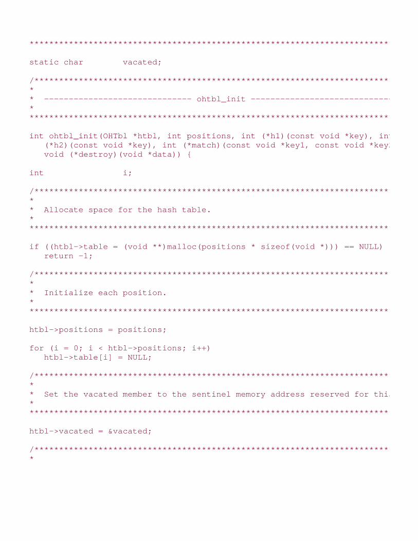
*****************************************************************************/
static char vacated;
/****************************************************************************** ** ------------------------------ ohtbl_init ------------------------------ ** ******************************************************************************/
int ohtbl_init(OHTbl *htbl, int positions, int (*h1)(const void *key), int (*h2)(const void *key), int (*match)(const void *key1, const void *key2), void (*destroy)(void *data)) {
int i;
/****************************************************************************** ** Allocate space for the hash table. ** ******************************************************************************/
if ((htbl->table = (void **)malloc(positions * sizeof(void *))) == NULL) return -1;
/****************************************************************************** ** Initialize each position. ** ******************************************************************************/
htbl->positions = positions;
for (i = 0; i < htbl->positions; i++) htbl->table[i] = NULL;
/****************************************************************************** ** Set the vacated member to the sentinel memory address reserved for this. ** ******************************************************************************/
htbl->vacated = &vacated;
/****************************************************************************** *

* Encapsulate the functions. ** ******************************************************************************/
htbl->h1 = h1;htbl->h2 = h2;htbl->match = match;htbl->destroy = destroy;
/****************************************************************************** ** Initialize the number of elements in the table. ** ******************************************************************************/
htbl->size = 0;
return 0;
}
/****************************************************************************** ** ---------------------------- ohtbl_destroy ----------------------------- ** ******************************************************************************/
void ohtbl_destroy(OHTbl *htbl) {
int i; if (htbl->destroy != NULL) {
/************************************************************************** * * * Call a user-defined function to free dynamically allocated data. * * * **************************************************************************/
for (i = 0; i < htbl->positions; i++) {
if (htbl->table[i] != NULL && htbl->table[i] != htbl->vacated) htbl->destroy(htbl->table[i]);
}

}
/****************************************************************************** ** Free the storage allocated for the hash table. ** ******************************************************************************/
free(htbl->table);
/****************************************************************************** ** No operations are allowed now, but clear the structure as a precaution. ** ******************************************************************************/
memset(htbl, 0, sizeof(OHTbl));
return;
}
/****************************************************************************** ** ----------------------------- ohtbl_insert ----------------------------- ** ******************************************************************************/
int ohtbl_insert(OHTbl *htbl, const void *data) {
void *temp;
int position, i; /****************************************************************************** ** Do not exceed the number of positions in the table. ** ******************************************************************************/
if (htbl->size == htbl->positions) return -1;
/****************************************************************************** *

* Do nothing if the data is already in the table. ** ******************************************************************************/
temp = (void *)data;
if (ohtbl_lookup(htbl, &temp) == 0) return 1;
/****************************************************************************** ** Use double hashing to hash the key. ** ******************************************************************************/
for (i = 0; i < htbl->positions; i++) {
position = (htbl->h1(data) + (i * htbl->h2(data))) % htbl->positions;
if (htbl->table[position] == NULL || htbl->table[position] == htbl-> vacated) {
/*********************************************************************** * * * Insert the data into the table. * * * ***********************************************************************/
htbl->table[position] = (void *)data; htbl->size++; return 0;
}
}
/****************************************************************************** ** Return that the hash functions were selected incorrectly. ** ******************************************************************************/
return -1;
}

/****************************************************************************** ** ----------------------------- ohtbl_remove ----------------------------- ** ******************************************************************************/
int ohtbl_remove(OHTbl *htbl, void **data) {
int position, i; /****************************************************************************** ** Use double hashing to hash the key. ** ******************************************************************************/
for (i = 0; i < htbl->positions; i++) {
position = (htbl->h1(*data) + (i * htbl->h2(*data))) % htbl->positions;
if (htbl->table[position] == NULL) {
/*********************************************************************** * * * Return that the data was not found. * * * ***********************************************************************/
return -1;
}
else if (htbl->table[position] == htbl->vacated) {
/*********************************************************************** * * * Search beyond vacated positions. * * * ***********************************************************************/
continue;
}
else if (htbl->match(htbl->table[position], *data)) {

/*********************************************************************** * * * Pass back the data from the table. * * * ***********************************************************************/
*data = htbl->table[position]; htbl->table[position] = htbl->vacated; htbl->size--; return 0;
}
}
/****************************************************************************** ** Return that the data was not found. ** ******************************************************************************/
return -1;
}
/****************************************************************************** ** ----------------------------- ohtbl_lookup ----------------------------- ** ******************************************************************************/
int ohtbl_lookup(const OHTbl *htbl, void **data) {
int position, i; /****************************************************************************** ** Use double hashing to hash the key. ** ******************************************************************************/
for (i = 0; i < htbl->positions; i++) {
position = (htbl->h1(*data) + (i * htbl->h2(*data))) % htbl->positions;

if (htbl->table[position] == NULL) {
/*********************************************************************** * * * Return that the data was not found. * * * ***********************************************************************/
return -1;
}
else if (htbl->match(htbl->table[position], *data)) {
/*********************************************************************** * * * Pass back the data from the table. * * * ***********************************************************************/
*data = htbl->table[position]; return 0;
}
}
/****************************************************************************** ** Return that the data was not found. ** ******************************************************************************/
return -1;
}
Top

Mastering Algorithms with CBy Kyle Loudon
Slots : 1
Table of Contents
Chapter 8. Hash Tables
Content
8.8 Questions and Answers
Q: In the implementation of chained hash tables presented in this chapter, the actual hash code usedfor accessing the table is the hash code modulo the table size. Why is this?
A: This transformation ensures that the hash coding does not position us past the end of the table.Although the hash function should ensure this itself, it is worthwhile for the hash tableimplementation to provide the guarantee as well, especially since the hash function is provided by thecaller. However, this is not the same reason that the modulo is performed when double hashing akey in an open-addressed hash table. In this case, the process of double hashing may produce ahash coding that falls outside of the bounds of the table, even for two auxiliary hash functions eachproducing hash codings within the table. This is because the two hash codings are added together.
Q: Why are hash tables good for random access but not sequential access? For example, in adatabase system in which records are to be accessed in a sequential fashion, what is the problemwith hashing?
A: Hash tables are excellent for random access because each key hashes us precisely to where weneed to be in the table to access the data, or at least within a few steps when a collision occurs.However, hash tables do not support sequential access. After hashing to some position, we have noway to determine where the next smallest or largest key resides. Compare this with a linked listcontaining elements that are sorted. Assuming some initial position in the list, the next key is easy todetermine: we simply look at the next element in the list.
Q: What is the worst-case performance of searching for an element in a chained hash table? How dowe ensure that this case will not occur?
A: A chained hash table performs the worst when all elements hash into a single bucket. In this case,searching for an element is O (n), where n is the number of elements in the table. A ridiculous hashfunction that would result in this performance is h (k) = c, where c is some constant within thebounds of the hash table. Selecting a good hash function ensures that this case will not occur. If thehash function approximates uniform hashing well, we can expect to locate an element in constanttime.
Q: What is the worst-case performance of searching for an element in an open-addressed hashtable? How do we ensure that this case will not occur?
A: The worst-case performance of searching for an element in an open-addressed hash table occurs

once the hash table is completely full and the element we are searching for is not in the table. In thiscase, searching for an element is an O (m) operation, where m is the number of positions in thetable. This case can occur with any hash function. To ensure reasonable performance in an open-addressed hash table, we should not let the table become more than 80% full. If we choose a hashfunction that approximates uniform hashing well, we can expect performance consistent with what ispresented in Table 8.1.
Top

Mastering Algorithms with CBy Kyle Loudon
Slots : 1
Table of Contents
Chapter 8. Hash Tables
Content
8.9 Related Topics
Direct-address tables
A simple type of hash table in which there is a one-to-one mapping between all possible keysand positions in the table. Since no two keys map to the same position, there is no need forcollision resolution. However, if there are many possible keys, the table will be large. Generally,direct addressing works well when the universe of possible keys is small.
Linear congruential generators
A common class of random number generators. Understanding the principles behind randomnumber generators can help in devising good hash functions.
Quadratic probing
An alternative to linear probing and double hashing for probing an open-addressed hash table.In quadratic probing, the sequence of positions probed is determined using a quadratic-formhash function. In general, quadratic probing performs better than linear probing, but it doesnot perform as well as double hashing. Quadratic probing results in secondary clustering, aform of clustering that is less severe than the primary clustering of linear probing.
Universal hashing
A hashing method in which hashing functions are generated randomly at runtime so that noparticular set of keys is likely to produce a bad distribution of elements in the hash table.Because the hash functions are generated randomly, even hashing the same set of keys duringdifferent executions may result in different measures of performance.
Top

Mastering Algorithms with CBy Kyle Loudon
Slots : 1
Table of Contents
Part II: Data Structures
Content
Chapter 9. TreesPicture a family tree, the draw sheet of a tournament, or the roots of a plant; these are all goodexamples of a tree's organization as a data structure. In computing, a tree consists of elementscalled nodes organized in a hierarchical arrangement. The node at the top of the hierarchy is calledthe root. The nodes directly below the root are its children, which in turn usually have children oftheir own. With the exception of the root, each node in the hierarchy has exactly one parent, which isthe node directly above it. The number of children a node may parent depends on the type of tree.This number is a tree's branching factor, which dictates how fast the tree will branch out as nodesare inserted. This chapter focuses on the binary tree, a relatively simple but powerful tree with abranching factor of 2. It also explores binary search trees, binary trees organized specifically forsearching.
This chapter covers:
Binary trees
Trees containing nodes with up to two children. The binary tree is a very popular type of treeutilized in a wide variety of problems. It provides the foundation for more sophisticated treestructures as well.
Traversal methods
Techniques for visiting the nodes of a tree in a specific order. Because the nodes of a tree areorganized in a hierarchical fashion, there are several options for traversing them.
Tree balancing
A process used to keep a tree as short as possible for a given number of nodes. This isespecially important in search trees, wherein height influences the overall performance of thetree a great deal.
Binary search trees
Binary trees organized specifically for searching. Binary search trees are good for searchingdata in which we expect to perform insertions and deletions.
Rotations
Methods for keeping binary search trees balanced. Specifically, this chapter explores AVLrotations, the rotations applied to AVL (Adel'son-Vel'skii and Landis) trees. An AVL tree is onetype of balanced binary search tree.

Some applications of trees are:
Huffman coding
A method of data compression that uses a Huffman tree to compress a set of data (seeChapter 14). A Huffman tree is a binary tree that determines the best way to assign codes tosymbols in the data. Symbols occurring frequently are assigned short codes, whereas symbolsoccurring less frequently are assigned longer ones.
User interfaces
Examples are graphical user interfaces and interfaces to file systems. In graphical userinterfaces, windows take on a hierarchical arrangement forming a tree. Every window, exceptthe top-level window, has one parent from which it is started, and each window may haveseveral children launched from it. Directories in hierarchical file systems have a similarorganization.
Database systems
In particular, those that require both efficient sequential and random access while performingfrequent insertions and deletions. The B-tree, a tree characterized generally as a balancedsearch tree with a large branching factor, is especially good in this situation (see the relatedtopics at the end of the chapter). Typically the branching factor of a B-tree is optimized so thatdisk I/O is minimized when accessing records in the database.
Expression processing (illustrated in this chapter)
A task performed frequently by compilers and hand-held calculators. One intuitive way toprocess arithmetic expressions is with an expression tree, a binary tree containing ahierarchical arrangement of an expression's operators and operands.
Artificial intelligence
A discipline that addresses many problems traditionally difficult for computers, such as logic-based games like chess. Many AI problems are solved using decision trees. A decision treeconsists of nodes that represent states in a problem. Each node is a point at which a decisionmust be made to continue. Each branch represents a conclusion derived from a series ofdecisions. Using various rules of logic, branches that cannot possibly contain desiredconclusions are pruned, thus decreasing the time to a solution.
Event schedulers
Applications for scheduling and triggering real-time events. Often real-time systems requirelooking up and retrieving the latest information associated with events as they are triggered. Abinary search tree can help make looking up information efficient.
Priority queues
Data structures that use a binary tree to keep track of which element in a set has the nexthighest priority (see Chapter 10). Priority queues offer a better solution than having to keep aset completely sorted.
Top

Mastering Algorithms with CBy Kyle Loudon
Slots : 1
Table of Contents
Chapter 9. Trees
Content
9.1 Description of Binary Trees
A binary tree is a hierarchical arrangement of nodes, each having up to two nodes immediately belowit. The nodes immediately below a node are called its children. The node above each child is called itsparent. Nodes can also have siblings, descendants, and ancestors. As you might expect, the siblingsof a node are the other children of its parent. The descendants of a node are all of the nodesbranching out below it. The ancestors of a node are all the nodes along the path between it and theroot. The performance associated with a tree often is discussed in terms of its height, the number oflevels in which nodes reside. As we will see, tree terminology is as much familial as it is arboreal (seeFigure 9.1).
Each node in a binary tree contains three parts: a data member and two pointers called the left andright pointers. Using this three-member structure, we form a binary tree by setting the left and rightpointers of each node to point to its children (see Figure 9.2). If a node does not have a child to itsleft or right, we set the appropriate pointer to NULL, a convenient sentinel that marks the end of abranch. A branch is a series of nodes beginning at the root and ending at a leaf node. Leaf nodes arethe nodes along the fringe of the tree that have no children. Sometimes when working with severaltrees at once, the trees are said to form a forest.
Figure 9.1. Common tree terminology illustrated with a four-level binarytree

Figure 9.2. Nodes linked together to form a binary tree
9.1.1 Traversal Methods
Traversing a binary tree means visiting its nodes one at a time in a specific order. Compared withsome linked data structures, such as linked lists, how to traverse the nodes of a binary tree may notbe immediately apparent. In fact, there are many ways in which we can proceed. Typically, one offour types of traversals is used: preorder, inorder, postorder, or level order. The example ofexpression trees later in this chapter presents recursive implementations of the preorder, inorder,and postorder traversals. For now, let's look at how each traversal works.
Traversing a tree is particularly simple if we think of the tree recursively as being composed of manysmaller subtrees. Figure 9.3 illustrates each traversal. Although these traversals are presented in thecontext of binary trees, each can be generalized to other types of trees as well.

9.1.1.1 Preorder traversal
In a preorder traversal for a given subtree, we first traverse its root, then to the left, and then to theright. As we explore subtrees to the left and right, we proceed in a similar manner using the left orright node as the root of the new subtree. The preorder traversal is a depth-first exploration, like thatpresented for graphs in Chapter 11.
9.1.1.2 Inorder traversal
In an inorder traversal for a given subtree, we first traverse to the left, then to the root, and then tothe right. As we explore subtrees to the left and right, we proceed in a similar manner using the leftor right node as the root of the new subtree.
9.1.1.3 Postorder traversal
In a postorder traversal for a given subtree, we first traverse to the left, then to the right, and thento the root. As we explore subtrees to the left and right, we proceed in a similar manner using theleft or right node as the root of the new subtree.
9.1.1.4 Level-order traversal
To traverse a binary tree in a level-order fashion, visit its nodes beginning at the root and proceeddownward, visiting the nodes at each level from left to right. The level-order traversal is a breadth-first exploration, like that presented for graphs in Chapter 11.
Figure 9.3. Traversing a binary tree in (a) preorder, (b) inorder, (c)postorder, and (d) level order

9.1.2 Tree Balancing
Balancing a tree is the process of keeping it as short as possible for a given number of nodes. Thismeans making sure that one level of the tree is completely full before allowing a node to exist at thenext level. Formally, a tree is balanced if all leaf nodes are at the same level or, if not, all leaf nodesare in the last two levels and the second-to-last level is full. For example, the tree in Figure 9.1 isbalanced because all leaf nodes are in the third and fourth levels, and the third level is full. On theother hand, the tree in Figure 9.3 is not balanced. A balanced tree is left-balanced if all leaves occupyonly the leftmost positions in the last level. The tree in Figure 9.4 is a left-balanced tree. We will seeone important application of balanced trees when binary search trees are discussed later in thischapter. In Chapter 10 we will see how a left-balanced binary tree helps to implement a heap andpriority queue.
Figure 9.4. A left-balanced binary tree

Top

Mastering Algorithms with CBy Kyle LoudonSlots : 1Table of ContentsChapter 9. Trees
Content
9.2 Interface for Binary Trees
This interface provides basic operations for manipulating binary trees. However, it does not provideoperations for inserting and removing individual nodes that are not leaves, because these operationsrequire adjusting other nodes in the tree in some application-specific way to accommodate the node that isinserted or removed.
bitree_init
void bitree_init(BiTree *tree, void (*destroy)(void *data));
Return Value
None.
Description
Initializes the binary tree specified by tree . This operation must be called for a binary tree before the
tree can be used with any other operation. The destroy argument provides a way to free dynamically
allocated data when bitree_destroy is called. For example, if the tree contains data dynamically allocated
using malloc , destroy should be set to free to free the data as the binary tree is destroyed. For
structured data containing several dynamically allocated members, destroy should be set to a user-
defined function that calls free for each dynamically allocated member as well as for the structure itself. For
a binary tree containing data that should not be freed, destroy should be set to NULL.
Complexity
O (1)
bitree_destroy

void bitree_destroy(BiTree *tree);
Return Value
None.
Description
Destroys the binary tree specified by tree . No other operations are permitted after calling bitree_destroy
unless bitree_init is called again. The bitree_destroy operation removes all nodes from a binary tree and
calls the function passed as destroy to bitree_init once for each node as it is removed, provided
destroy was not set to NULL.
Complexity
O (n ), where n is the number of nodes in the binary tree.
bitree_ins_left
int bitree_ins_left(BiTree *tree, BiTreeNode *node, const void *data);
Return Value
0if inserting the node is successful, or -1 otherwise.
Description
Inserts a node as the left child of node in the binary tree specified by tree . If node already has a left
child, bitree_ins_left returns -1. If node is NULL, the new node is inserted as the root node. The tree must
be empty to insert a node as the root node; otherwise, bitree_ins_left returns -1. When successful, the new
node contains a pointer to data , so the memory referenced by data should remain valid as long as the
node remains in the binary tree. It is the responsibility of the caller to manage the storage associated with
data .
Complexity
O (1)
bitree_ins_right
int bitree_ins_right(BiTree *tree, BiTreeNode *node, const void *data);

Return Value
0if inserting the node is successful, or -1 otherwise.
Description
This operation is similar to bitree_ins_left , except that it inserts a node as the right child of node in the
binary tree specified by tree .
Complexity
O (1)
bitree_rem_left
void bitree_rem_left(BiTree *tree, BiTreeNode *node);
Return Value
None.
Description
Removes the subtree rooted at the left child of node from the binary tree specified by tree . If node is
NULL, all nodes in the tree are removed. The function passed as destroy to bitree_init is called once for
each node as it is removed, provided destroy was not set to NULL.
Complexity
O (n ), where n is the number of nodes in the subtree.
bitree_rem_right
void bitree_rem_right(BiTree *tree, BiTreeNode *node);
Return Value
None.
Description
This operation is similar to bitree_rem_left , except that it removes the subtree rooted at the right child of
node from the binary tree specified by tree .

Complexity
O (n ), where n is the number of nodes in the subtree.
bitree_merge
int bitree_merge(BiTree *merge, BiTree *left, BiTree *right, const void *data);
Return Value
0if merging the trees is successful, or -1 otherwise.
Description
Merges the two binary trees specified by left and right into the single binary tree merge . After
merging is complete, merge contains data in its root node, and left and right are the left and
right subtrees of its root. Once the trees have been merged, left and right are as if bitree_destroy
had been called on them.
Complexity
O (1)
bitree_size
int bitree_size(const BiTree *tree);
Return Value
Number of nodes in the tree.
Description
Macro that evaluates to the number of nodes in the binary tree specified by tree .
Complexity
O (1)
bitree_root
BiTreeNode *bitree_root(const BiTree *tree);
Return Value

Node at the root of the tree.
Description
Macro that evaluates to the node at the root of the binary tree specified by tree .
Complexity
O (1)
bitree_is_eob
int bitree_is_eob(const BiTreeNode *node);
Return Value
1 if the node marks the end of a branch, or otherwise.
Description
Macro that determines whether the node specified as node marks the end of a branch in a binary tree.
Complexity
O (1)
bitree_is_leaf
int bitree_isleaf(const BiTreeNode *node);
Return Value
1 if the node is a leaf node, or otherwise.
Description
Macro that determines whether the node specified as node is a leaf node in a binary tree.
Complexity
O (1)
bitree_data

void *bitree_data(const BiTreeNode *node);
Return Value
Data stored in the node.
Description
Macro that evaluates to the data stored in the node of a binary tree specified by node .
Complexity
O (1)
bitree_left
BiTreeNode *bitree_left(const BiTreeNode *node);
Return Value
Left child of the specified node.
Description
Macro that evaluates to the node of a binary tree that is the left child of the node specified by node .
Complexity
O (1)
bitree_right
BiTreeNode *bitree_right(const BiTreeNode *node);
Return Value
Right child of the specified node.
Description
Macro that evaluates to the node of a binary tree that is the right child of the node specified by node .
Complexity

O (1)
Top

Mastering Algorithms with CBy Kyle LoudonSlots : 1Table of ContentsChapter 9. Trees
Content
9.3 Implementation and Analysis of Binary Trees
Recall that each node of a binary tree consists of three parts: a data member and two pointers to its
children. The structure BiTreeNode represents an individual node of a binary tree (see Example 9.1 ).
As you would expect, this structure has three members that correspond to those just mentioned. The
structure BiTree is the binary tree data structure (see Example 9.1 ). This structure consists of four
members: size is the number of nodes in the tree, compare is a member not used by binary trees but
by datatypes that will be derived later from binary trees, destroy is the encapsulated destroy function
passed to bitree_init , and root is a pointer to the top of the node hierarchy.
Example 9.1. Header for the Binary Tree Abstract Datatype
/****************************************************************************** ** ------------------------------- bitree.h ------------------------------- ** ******************************************************************************/
#ifndef BITREE_H#define BITREE_H
#include <stdlib.h>
/****************************************************************************** ** Define a structure for binary tree nodes. ** ******************************************************************************/

typedef struct BiTreeNode_ {
void *data;struct BiTreeNode_ *left;struct BiTreeNode_ *right; } BiTreeNode;
/****************************************************************************** ** Define a structure for binary trees. ** ******************************************************************************/
typedef struct BiTree_ {
int size;
int (*compare)(const void *key1, const void *key2);void (*destroy)(void *data);
BiTreeNode *root;
} BiTree;
/****************************************************************************** ** --------------------------- Public Interface --------------------------- ** ******************************************************************************/
void bitree_init(BiTree *tree, void (*destroy)(void *data));
void bitree_destroy(BiTree *tree);
int bitree_ins_left(BiTree *tree, BiTreeNode *node, const void *data);
int bitree_ins_right(BiTree *tree, BiTreeNode *node, const void *data);
void bitree_rem_left(BiTree *tree, BiTreeNode *node);
void bitree_rem_right(BiTree *tree, BiTreeNode *node);
int bitree_merge(BiTree *merge, BiTree *left, BiTree *right, const void *data);
#define bitree_size(tree) ((tree)->size)

#define bitree_root(tree) ((tree)->root)
#define bitree_is_eob(node) ((node) == NULL)
#define bitree_is_leaf(node) ((node)->left == NULL && (node)->right == NULL)
#define bitree_data(node) ((node)->data)
#define bitree_left(node) ((node)->left)
#define bitree_right(node) ((node)->right)
#endif
9.3.1 bitree_init
The bitree_init operation initializes a binary tree so that it can be used in other operations (see Example 9.2
). Initializing a binary tree is a simple operation in which we set the size member of the tree to 0, the
destroy member to destroy , and the root pointer to NULL.
The runtime complexity of bitree_init is O (1) because all of the steps in initializing a binary tree run in aconstant amount of time.
9.3.2 bitree_destroy
The bitree_destroy operation destroys a binary tree (see Example 9.2 ). Primarily this means removing all
nodes from the tree. The function passed as destroy to bitree_init is called once for each node as it is
removed, provided destroy was not set to NULL.
The runtime complexity of bitree_destroy is O (n ), where n is the number of nodes in the binary tree. Thisis because bitree_destroy simply calls bitree_rem_left , which runs in O (n ) time, where n is the number ofnodes in the tree.
9.3.3 bitree_ins_left
The bitree_ins_left operation inserts a node into a binary tree as the left child of a specified node (seeExample 9.2 ). The call sets the new node to point to the data passed by the caller. Linking the new node
into the tree is accomplished by setting the left pointer of node to point to the new node. If node is
NULL and the tree is empty, we set the root member of the tree data structure to the new node. We
update the size of the tree by incrementing the size member.
The runtime complexity of bitree_ins_left is O (1) because all of the steps in inserting a node into a binarytree run in a constant amount of time.
9.3.4 bitree_ins_right

The bitree_ins_right operation inserts a node into a binary tree as the right child of a specified node (seeExample 9.2 ). This operation works similarly to bitree_ins_left , except that linking the new node into the
tree is accomplished by setting the right pointer of node to point to the new node.
The runtime complexity of bitree_ins_right is O (1) because all of the steps in inserting a node into a binarytree run in a constant amount of time.
9.3.5 bitree_rem_left
The bitree_rem_left operation removes the subtree rooted at the left child of a specified node (see Example
9.2 ). Nodes are removed by performing a postorder traversal beginning at the left child of node . If
node is NULL, we begin the traversal at the root node. The function passed as destroy to bitree_init is
called once for each node as it is removed, provided destroy was not set to NULL. As each node is
removed, we update the size member of the tree data structure as well.
The runtime complexity of bitree_rem_left is O (n ), where n is the number of nodes in the subtree rooted
at the left child of node . This is because bitree_rem_left performs a postorder traversal to visit each of
the nodes in the subtree while all other parts of the operation run in a constant amount of time.
9.3.6 bitree_rem_right
The bitree_rem_right operation removes the subtree rooted at the right child of a specified node (seeExample 9.2 ). This operation works much like bitree_rem_left , except that nodes are removed by
performing a postorder traversal beginning at the right child of node .
The runtime complexity of bitree_rem_right is O (n ), where n is the number of nodes in the subtree rooted
at the right child of node . This is because bitree_rem_right performs a postorder traversal to visit each of
the nodes in the subtree while all other parts of the operation run in a constant amount of time.
9.3.7 bitree_merge
The bitree_merge operation merges two binary trees into a single binary tree (see Example 9.2 ). First, we
initialize merge by calling bitree_init . Next, we insert data into the merged tree at its root. The merged
tree's left and right children are then set to be the root nodes of left and right , and the size of the
tree is adjusted to reflect the sizes of the subtrees. Last, we detach the nodes now in the merged tree fromthe original trees and set the size of each tree to 0.
The runtime complexity of bitree_merge is O (1) because all of the steps in merging two binary trees run ina constant amount of time.
9.3.8 bitree_size, bitree_root, bitree_is_eob, bitree_is_leaf, bitree_data,bitree_left, bitree_right
These macros implement some of the simpler binary tree operations (see Example 9.1 ). Generally, they
provide an interface for accessing and testing members of the BiTree and BiTreeNode structures.
The runtime complexity of these operations is O (1) because accessing and testing members of a structure

are simple tasks that run in a constant amount of time.
Example 9.2. Implementation of the Binary Tree Abstract Datatype
/****************************************************************************** ** ------------------------------- bitree.c ------------------------------- ** ******************************************************************************/
#include <stdlib.h>#include <string.h>
#include "bitree.h"
/****************************************************************************** ** ------------------------------ bitree_init ----------------------------- ** ******************************************************************************/
void bitree_init(BiTree *tree, void (*destroy)(void *data)) {
/****************************************************************************** ** Initialize the binary tree. ** ******************************************************************************/
tree->size = 0;tree->destroy = destroy;tree->root = NULL;
return;
}
/****************************************************************************** ** ---------------------------- bitree_destroy ---------------------------- ** ******************************************************************************/
void bitree_destroy(BiTree *tree) {
/*****************************************************************************
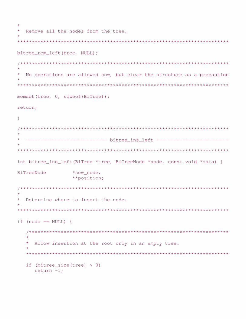
* ** Remove all the nodes from the tree. ** ******************************************************************************/
bitree_rem_left(tree, NULL);
/****************************************************************************** ** No operations are allowed now, but clear the structure as a precaution. ** ******************************************************************************/
memset(tree, 0, sizeof(BiTree));
return;
}
/****************************************************************************** ** ---------------------------- bitree_ins_left --------------------------- ** ******************************************************************************/
int bitree_ins_left(BiTree *tree, BiTreeNode *node, const void *data) {
BiTreeNode *new_node, **position;
/****************************************************************************** ** Determine where to insert the node. ** ******************************************************************************/
if (node == NULL) {
/************************************************************************** * * * Allow insertion at the root only in an empty tree. * * * **************************************************************************/
if (bitree_size(tree) > 0) return -1;

position = &tree->root;
}
else {
/************************************************************************** * * * Normally allow insertion only at the end of a branch. * * * **************************************************************************/
if (bitree_left(node) != NULL) return -1;
position = &node->left;
}
/****************************************************************************** ** Allocate storage for the node. ** ******************************************************************************/
if ((new_node = (BiTreeNode *)malloc(sizeof(BiTreeNode))) == NULL) return -1;
/****************************************************************************** ** Insert the node into the tree. ** ******************************************************************************/
new_node->data = (void *)data;new_node->left = NULL;new_node->right = NULL;*position = new_node;
/****************************************************************************** ** Adjust the size of the tree to account for the inserted node. ** ******************************************************************************/
tree->size++;

return 0;
}
/****************************************************************************** ** --------------------------- bitree_ins_right --------------------------- ** ******************************************************************************/
int bitree_ins_right(BiTree *tree, BiTreeNode *node, const void *data) {
BiTreeNode *new_node, **position;
/****************************************************************************** ** Determine where to insert the node. ** ******************************************************************************/
if (node == NULL) {
/************************************************************************** * * * Allow insertion at the root only in an empty tree. * * * **************************************************************************/
if (bitree_size(tree) > 0) return -1;
position = &tree->root;
}
else {
/************************************************************************** * * * Normally allow insertion only at the end of a branch. * * * **************************************************************************/
if (bitree_right(node) != NULL)

return -1;
position = &node->right;
}
/****************************************************************************** ** Allocate storage for the node. ** ******************************************************************************/
if ((new_node = (BiTreeNode *)malloc(sizeof(BiTreeNode))) == NULL) return -1;
/****************************************************************************** ** Insert the node into the tree. ** ******************************************************************************/
new_node->data = (void *)data;new_node->left = NULL;new_node->right = NULL;*position = new_node;
/****************************************************************************** ** Adjust the size of the tree to account for the inserted node. ** ******************************************************************************/
tree->size++;
return 0;
}
/****************************************************************************** ** ---------------------------- bitree_rem_left --------------------------- ** ******************************************************************************/
void bitree_rem_left(BiTree *tree, BiTreeNode *node) {
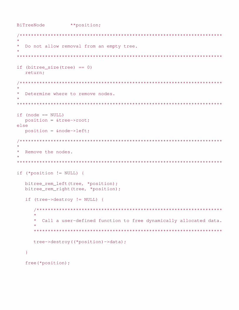
BiTreeNode **position;
/****************************************************************************** ** Do not allow removal from an empty tree. ** ******************************************************************************/
if (bitree_size(tree) == 0) return;
/****************************************************************************** ** Determine where to remove nodes. ** ******************************************************************************/
if (node == NULL) position = &tree->root;else position = &node->left;
/****************************************************************************** ** Remove the nodes. ** ******************************************************************************/
if (*position != NULL) {
bitree_rem_left(tree, *position); bitree_rem_right(tree, *position);
if (tree->destroy != NULL) {
/*********************************************************************** * * * Call a user-defined function to free dynamically allocated data. * * * ***********************************************************************/
tree->destroy((*position)->data);
}
free(*position);

*position = NULL;
/************************************************************************** * * * Adjust the size of the tree to account for the removed node. * * * **************************************************************************/
tree->size--;
}
return;
}
/****************************************************************************** ** --------------------------- bitree_rem_right --------------------------- ** ******************************************************************************/
void bitree_rem_right(BiTree *tree, BiTreeNode *node) {
BiTreeNode **position;
/****************************************************************************** ** Do not allow removal from an empty tree. ** ******************************************************************************/
if (bitree_size(tree) == 0) return;
/****************************************************************************** ** Determine where to remove nodes. ** ******************************************************************************/
if (node == NULL) position = &tree->root;else position = &node->right;

/****************************************************************************** ** Remove the nodes. ** ******************************************************************************/
if (*position != NULL) {
bitree_rem_left(tree, *position); bitree_rem_right(tree, *position);
if (tree->destroy != NULL) {
/*********************************************************************** * * * Call a user-defined function to free dynamically allocated data. * * * ***********************************************************************/
tree->destroy((*position)->data);
}
free(*position); *position = NULL;
/************************************************************************** * * * Adjust the size of the tree to account for the removed node. * * * **************************************************************************/
tree->size--;
}
return;
}
/****************************************************************************** ** ----------------------------- bitree_merge ----------------------------- ** ******************************************************************************/

int bitree_merge(BiTree *merge, BiTree *left, BiTree *right, const void *data) {
/****************************************************************************** ** Initialize the merged tree. ** ******************************************************************************/
bitree_init(merge, left->destroy);
/****************************************************************************** ** Insert the data for the root node of the merged tree. ** ******************************************************************************/
if (bitree_ins_left(merge, NULL, data) != 0) {
bitree_destroy(merge); return -1;
}
/****************************************************************************** ** Merge the two binary trees into a single binary tree. ** ******************************************************************************/
bitree_root(merge)->left = bitree_root(left);bitree_root(merge)->right = bitree_root(right);
/****************************************************************************** ** Adjust the size of the new binary tree. ** ******************************************************************************/
merge->size = merge->size + bitree_size(left) + bitree_size(right);
/****************************************************************************** ** Do not let the original trees access the merged nodes. ** ******************************************************************************/

left->root = NULL;left->size = 0;right->root = NULL;right->size = 0;
return 0;
}
Top

Mastering Algorithms with CBy Kyle LoudonSlots : 1Table of ContentsChapter 9. Trees
Content
9.4 Binary Tree Example: Expression Processing
One intuitive way to process arithmetic expressions with a computer is using an expression tree . Anexpression tree is a binary tree consisting of nodes containing two types of objects: operators and terminalvalues . Operators are objects that have operands; terminal values are objects that have no operands.
The idea behind an expression tree is simple: the subtrees rooted at the children of each node are theoperands of the operator stored in the parent (see Figure 9.5 ). Operands may be terminal values, or theymay be other expressions themselves. Expressions are expanded in subtrees; terminal values reside in leafnodes. One of the nice things about this idea is how easily an expression tree allows us to translate anexpression into one of three common representations: prefix , infix , and postfix . To obtain theserepresentations, we simply traverse the tree using a preorder, inorder, or postorder traversal.
Traversing the tree in Figure 9.5 in preorder, for example, yields the prefix expression x / - 74 10 32 + 2317. To evaluate a prefix expression, we apply each operator to the two operands that immediately follow it.Thus, the prefix expression just given is evaluated as:
( x ( / ( - 74 10 ) 32 ) ( + 23 17 ) ) = 80
Infix expressions are the expressions we are most familiar with from mathematics, but they are not wellsuited to processing by a computer. If we traverse the tree of Figure 9.5 using an inorder traversal, we getthe infix expression 74 - 10 / 32 x 23 + 17. Notice that one of the difficulties with infix expressions is thatthey do not inherently identify in which order operations should be performed, whereas prefix and postfixexpressions do. However, we can remedy this situation in an infix expression by parenthesizing each part ofthe expression as we traverse it in the tree. Fully parenthesized, the previous infix expression is evaluatedas:
( ( ( 74 - 10 ) / 32 ) x ( 23 + 17 ) ) = 80
Postfix expressions are well suited to processing by a computer. If we traverse the tree of Figure 9.5 inpostorder, we get the postfix expression 74 10 - 32 / 23 17 + x. To evaluate a postfix expression, we applyeach operator to the two operands immediately preceding it. Thus, the postfix expression just given isevaluated as:

( ( ( 74 10 - ) 32 /) ( 23 17 + ) x ) = 80
Figure 9.5. An expression tree for the expression ((74 - 10) / 32) x (23 + 17)
One reason postfix expressions are well suited to computers is that they are easy to evaluate with anabstract stack machine , an abstraction used by compilers and hand-held calculators. To process a postfixexpression using an abstract stack machine, we proceed as follows. First, we move from left to rightthrough the expression, pushing values onto the stack until an operator is encountered. Next, the operandsrequired by the operator are popped, the operator is applied to them, and the result is pushed back on thestack. This procedure is repeated until the entire expression has been processed, at which point the valueof the expression is the lone item remaining on the stack (see Figure 9.6 ).
Figure 9.6. An abstract stack machine processing the postfix expression 7410 - 32 / 23 17 + x
Example 9.3 illustrates how to produce the prefix, infix, and postfix representations of an expression storedin an expression tree. For this, three functions are provided, preorder , inorder , and postorder , whichtraverse a binary tree in preorder, inorder, and postorder, respectively. Each function accepts two
arguments: node and list .
To begin a traversal, we set node to the root node of the expression tree we wish to traverse. Successive
recursive calls set node to the node at the top of the subtree about to be traversed. On the initial call to
each function, we also pass into list an empty linked list already initialized with list_init . For each of the
traversals, nodes are placed into the list in the order they are encountered. When the initial call in the

recursion returns, list contains the preorder, inorder, or postorder listing of the nodes, as appropriate.
Notice how a recursive implementation of these traversals nicely models the definitions presented earlier inthe chapter.
Example 9.3. Implementation of Functions for Traversing a Binary Tree
/****************************************************************************** ** ------------------------------ traverse.c ------------------------------ ** ******************************************************************************/
#include "list.h"#include "traverse.h"
/****************************************************************************** ** ------------------------------- preorder ------------------------------- ** ******************************************************************************/
int preorder(const BiTreeNode *node, List *list) {
/****************************************************************************** ** Load the list with a preorder listing of the tree. ** ******************************************************************************/
if (!bitree_is_eob(node)) {
if (list_ins_next(list, list_tail(list), bitree_data(node)) != 0) return -1;
if (!bitree_is_eob(bitree_left(node))) if (preorder(bitree_left(node), list) != 0) return -1;
if (!bitree_is_eob(bitree_right(node))) if (preorder(bitree_right(node), list) != 0) return -1;
}
return 0;

}
/****************************************************************************** ** -------------------------------- inorder ------------------------------- ** ******************************************************************************/
int inorder(const BiTreeNode *node, List *list) {
/****************************************************************************** ** Load the list with an inorder listing of the tree. ** ******************************************************************************/
if (!bitree_is_eob(node)) {
if (!bitree_is_eob(bitree_left(node))) if (inorder(bitree_left(node), list) != 0) return -1;
if (list_ins_next(list, list_tail(list), bitree_data(node)) != 0) return -1;
if (!bitree_is_eob(bitree_right(node))) if (inorder(bitree_right(node), list) != 0) return -1;
}
return 0;
}
/****************************************************************************** ** ------------------------------- postorder ------------------------------ ** ******************************************************************************/
int postorder(const BiTreeNode *node, List *list) {
/****************************************************************************** ** Load the list with a postorder listing of the tree. *

* ******************************************************************************/
if (!bitree_is_eob(node)) {
if (!bitree_is_eob(bitree_left(node))) if (postorder(bitree_left(node), list) != 0) return -1;
if (!bitree_is_eob(bitree_right(node))) if (postorder(bitree_right(node), list) != 0) return -1;
if (list_ins_next(list, list_tail(list), bitree_data(node)) != 0) return -1;
}
return 0;
}
Top

Mastering Algorithms with CBy Kyle Loudon
Slots : 1
Table of Contents
Chapter 9. Trees
Content
9.5 Description of Binary Search Trees
Binary search trees are binary trees organized specifically for searching. To search for a node in abinary search tree, we start at the root of the tree and descend level by level until we find the nodewe are looking for. When we encounter a node greater than the desired node, we follow its leftpointer. When we encounter a node that is less, we follow its right pointer. For example, to locate 15in the tree of Figure 9.7, start at the root and move to the left since 15 is less than 20, then to theright since 15 is greater than 09, at which point we find 15. If we reach the end of a branch beforelocating the desired node, it does not exist.
Of course, the process of searching a binary tree depends on nodes having been inserted in a similarway. Thus, to insert a node, we start at the root of the tree and descend level by level, moving left orright as appropriate. When we reach the end of a branch, we make the insertion. For example, toinsert 65 into the tree of Figure 9.7, we start at the root and move to the right since 65 is greaterthan 20, then to the right again since 65 is greater than 53, and then to the left since 65 is less than79. This point is the end of a branch, so we insert the key as the left child of 79. Duplicate keys arenot allowed.
Figure 9.7. A binary search tree, including the paths traced while locating15 and inserting 65
Binary search trees are efficient structures for searching because in the worst case, we only end upsearching the data in one branch, instead of having to search every piece of data. Thus, searching

becomes an O (lg n) operation, where n is the number of nodes in the tree, provided the tree is keptbalanced. Recall that keeping a tree balanced means that it will be as short as possible for a givennumber of nodes. Keeping a binary search tree balanced is important because it means that nobranch we search will be exceptionally long.
To understand further the importance of keeping a binary search tree balanced, consider whathappens as a binary search tree becomes more and more unbalanced. As this occurs, searching for anode approaches O (n), which is no better than searching from one end of the data to the next. Forexample, imagine a binary search tree containing 216 words from a dictionary inserted inalphabetical order (see Figure 9.8). In this case, the tree consists of a single branch to the right, andsearching for a word could require inspecting as many as 216 words. However, if we insert the wordsin a random fashion, the tree should end up at least somewhat balanced, and we can expect totraverse closer to lg 216 = 16 words in the worst case. Since normally the order in which nodes areinserted and removed is not something we can control, we cannot rely on this method to keep a treebalanced. Instead, we must take a more proactive approach.
Figure 9.8. A poorly balanced binary search tree consisting of a singlebranch to the right
Top

Mastering Algorithms with CBy Kyle Loudon
Slots : 1
Table of Contents
Chapter 9. Trees
Content
9.6 Interface for Binary Search Trees
bistree_init
void bistree_init(BisTree *tree, void (*compare)(const void *key1, const void *key2), void (*destroy)(void *data));
Return Value
None.
Description
Initializes the binary search tree specified by tree. This operation must be called for a binary searchtree before the tree can be used with any other operation. The function pointer compare specifies auser-defined function to compare elements. This function should return 1 if key1 > key2, if key1 =key2, and -1 if key1 < key2. The destroy argument provides a way to free dynamicallyallocated data when bistree_destroy is called. It works in a manner similar to that described forbitree_destroy. For a binary search tree containing data that should not be freed, destroy shouldbe set to NULL.
Complexity
O (1)
bistree_destroy
void bistree_destroy(BisTree *tree);
Return Value

None.
Description
Destroys the binary search tree specified by tree. No other operations are permitted after callingbistree_destroy unless bistree_init is called again. The bistree_destroy operation removes all nodesfrom a binary search tree and calls the function passed as destroy to bistree_init once for eachnode as it is removed, provided destroy was not set to NULL.
Complexity
O (n), where n is the number of nodes in the binary search tree.
bistree_insert
int bistree_insert(BisTree *tree, const void *data);
Return Value
0 if inserting the node is successful, 1 if the node is already in the tree, or -1 otherwise.
Description
Inserts a node into the binary search tree specified by tree. The new node contains a pointer todata, so the memory referenced by data should remain valid as long as the node remains in thebinary search tree. It is the responsibility of the caller to manage the storage associated with data.
Complexity
O (lg n), where n is the number of nodes in the binary search tree.
bistree_remove
int bistree_remove(BisTree *tree, const void *data);
Return Value
0if removing the node is successful, or -1 otherwise.
Description

Removes the node matching data from the binary search tree specified by tree. In actuality, thisoperation only performs a lazy removal, in which the node is simply marked as hidden. Thus, nopointer is returned to the data matching data. Furthermore, the data in the tree must remain valideven after it has been removed. Consequently, the size of the binary search tree, as returned bybistree_size, does not decrease after removing a node. This approach is explained further in theimplementation and analysis section.
Complexity
O (lg n), where n is the number of nodes in the binary search tree.
bistree_lookup
int bistree_lookup(const BisTree *tree, void **data);
Return Value
0if the data is found in the binary search tree, or -1 otherwise.
Description
Determines whether a node matches data in the binary search tree specified as tree. If a match isfound, data points to the matching data in the binary search tree upon return.
Complexity
O (lg n), where n is the number of nodes in the binary search tree.
bistree_size
int bistree_size(const BisTree *tree);
Return Value
Number of nodes in the tree.
Description
Macro that evaluates to the number of nodes in the binary search tree specified by tree.

Complexity
O (1)
Top

Mastering Algorithms with CBy Kyle LoudonSlots : 1Table of ContentsChapter 9. Trees
Content
9.7 Implementation and Analysis of Binary Search Trees
As described earlier, binary search trees perform well only if the tree remains balanced. Unfortunately,keeping a binary search tree balanced is a more difficult problem than it may at first appear. Nevertheless,there are a few clever approaches one can take. One of the best approaches is to implement the tree as anAVL tree .
An AVL (Adel'son-Vel'skii and Landis) tree is a special type of binary tree that stores an extra piece ofinformation with each node: its balance factor . The balance factor of a node is the height of the subtreerooted at its left child minus the height of the subtree rooted at its right child (see Figure 9.9 ). As nodesare inserted, an AVL tree adjusts itself so that all balance factors stay +1, -1, or 0. A subtree whose rootnode has a balance factor of +1 is said to be left-heavy . A subtree whose root node has a balance factor of-1 is said to be right-heavy . A subtree whose root node has a balance factor of is considered balanced. Bykeeping its subtrees nearly balanced, an AVL tree stays approximately balanced overall.
Figure 9.9. An AVL tree, including balance factors
The basic means of searching and inserting nodes in an AVL tree is the same as described earlier. However,when we insert a node into an AVL tree, we have some additional work to do after the node descends to its

appropriate position. First, we must account for the change in balance factors that occurs as a result of theinsertion. Also, if any balance factor becomes ±2, we must rebalance the tree from that point down, whichis done by performing an operation called a rotation .
9.7.1 Rotations in AVL Trees
A rotation rebalances part of an AVL tree by rearranging nodes while preserving the relationship whereinthe left is smaller than the parent and the parent is smaller than the right, which must be maintained forthe tree to remain a binary search tree. After the rotation, the balance factors of all nodes in the rotatedsubtree are +1, -1, or 0.
There are only four types of rotations that ever have to be performed. These are the LL (left-left ), LR (left-right ), RR (right-right ), and RL (right-left ) rotations. The functions rotate_left and rotate_right ,presented later in Example 9.5 , implement each of these rotations. To understand when we need to applyeach rotation, let x represent the node we have just inserted into its proper location in an AVL tree, and letA be the nearest ancestor of x whose balance factor has changed to ±2.
9.7.1.1 LL rotation
We perform an LL, or left-left, rotation when x lies in the left subtree of the left subtree of A (see Figure9.10 ). Let left be the left child of A . To perform an LL rotation, we set the left pointer of A to the rightchild of left , the right pointer of left to A , and the pointer referencing A to left . After the rotation, we setthe balance factors of both A and left to 0. All other balance factors do not change.
Figure 9.10. An LL rotation in an AVL tree
9.7.1.2 LR rotation

We perform an LR, or left-right, rotation when x lies in the right subtree of the left subtree of A (see Figure9.11 ). Let left be the left child of A and grandchild be the right child of left . To perform an LR rotation, weset the right child of left to the left child of grandchild , the left child of grandchild to left , the left child of Ato the right child of grandchild , the right child of grandchild to A , and finally the pointer referencing A tograndchild .
Figure 9.11. An LR rotation in an AVL tree
Adjusting the balance factors of nodes after an LR rotation depends on the original balance factor ofgrandchild . Figure 9.12 illustrates the three cases to consider. If the original balance factor of grandchildwas +1, we set the balance factor of A to -1 and left to 0. If the original balance factor of grandchild was 0,we set the balance factors of both A and left to 0. If the original balance factor of grandchild was -1, we setthe balance factor of A to and that of left to +1. In all cases, we set the new balance factor of grandchild to0. All other balance factors do not change.
Figure 9.12. Updating balance factors after an LR rotation in an AVL tree

9.7.1.3 RR rotation
We perform an RR, or right-right, rotation when x lies in the right subtree of the right subtree of A . The RRrotation is symmetric to the LL rotation. Let right be the right child of A . To perform an RR rotation, we setthe right pointer of A to the left child of right , the left pointer of right to A , and the pointer referencing A toright . After the rotation, we set the balance factors of both A and left to 0. All other balance factors do notchange.
9.7.1.4 RL rotation
We perform an RL, or right-left, rotation when x lies in the left subtree of the right subtree of A . The RLrotation is symmetric to the LR rotation. Let right be the right child of A and grandchild be the left child ofright . To perform an RL rotation, we set the left child of right to the right child of grandchild , the rightchild of grandchild to right , the right child of A to the left child of grandchild , the left child of grandchild to

A , and finally the pointer referencing A to grandchild .
Adjusting the balance factors of nodes after an RL rotation depends on the original balance factor ofgrandchild . There are three cases to consider. If the original balance factor of grandchild was +1, we setthe balance factor of A to and that of right to -1. If the original balance factor of grandchild was 0, we setthe balance factors of both A and left to 0. If the original balance factor of grandchild was -1, we set thebalance factor of A to +1 and that of left to 0. In all cases, we set the new balance factor of grandchild to0. All other balance factors do not change. These adjustments are symmetric to those shown in Figure 9.12for an LR rotation.
The structure BisTree is the binary search tree data structure. A good way to implement a binary
search tree is to use the binary tree abstract datatype discussed earlier. Thus, BisTree is implemented
as a typedef to BiTree (see Example 9.4 ). In addition to simplicity, using a typedef has the benefit of
making the binary search tree somewhat polymorphic, just as described for stacks and queues (seeChapter 6 ). This means that we can use binary tree operations on a binary search tree in addition to thoseoperations defined specifically for binary search trees.
Since keeping a binary search tree balanced requires that each node store more than just the data placed
in the tree, a structure, AvlNode , is defined for each node to contain (see Example 9.4 ). An AvlNodestructure consists of three members: data is the data stored in the node, hidden is a member used to
mark a node when it is removed, and factor is the node's balance factor. The implementation presented
here also uses identifiers to represent the possible values for balance factors. Example 9.4 equates
AVL_LEFT_HEAVY to 1, AVL_BALANCED to 0, and AVL_RGT_HEAVY to -1.
Example 9.4. Header for the Binary Search Tree Abstract Datatype
/****************************************************************************** ** ------------------------------- bistree.h ------------------------------ ** ******************************************************************************/
#ifndef BISTREE_H#define BISTREE_H
#include "bitree.h"
/****************************************************************************** ** Define balance factors for AVL trees. ** ******************************************************************************/
#define AVL_LFT_HEAVY 1#define AVL_BALANCED 0#define AVL_RGT_HEAVY -1
/*****************************************************************************

* ** Define a structure for nodes in AVL trees. ** ******************************************************************************/
typedef struct AvlNode_ {
void *data;int hidden;int factor;
} AvlNode;
/****************************************************************************** ** Implement binary search trees as binary trees. ** ******************************************************************************/
typedef BiTree BisTree;
/****************************************************************************** ** --------------------------- Public Interface --------------------------- ** ******************************************************************************/
void bistree_init(BisTree *tree, int (*compare)(const void *key1, const void *key2), void (*destroy)(void *data));
void bistree_destroy(BisTree *tree);
int bistree_insert(BisTree *tree, const void *data);
int bistree_remove(BisTree *tree, const void *data);
int bistree_lookup(BisTree *tree, void **data);
#define bistree_size(tree) ((tree)->size)
#endif
9.7.2 bistree_init
The bistree_init operation initializes a binary search tree so that it can be used in other operations (see
Example 9.5 ). Since a binary search tree is a binary tree, we call bitree_init to initialize it. The compare

member is set to compare by hand because this member is not used by binary trees and therefore is not
set by bitree_init .
The runtime complexity of bistree_init is the same as bitree_init , or O (1).
9.7.3 bistree_destroy
The bistree_destroy operation destroys a binary search tree (see Example 9.5 ). To do this, we employ thesupport of two additional functions, destroy_left and destroy_right , which recursively destroy the left andright subtrees beneath a node. These functions work similarly to the bitree_rem_left and bitree_rem_rightfunctions defined previously for binary trees. Separate functions are required for binary search trees so that
we can destroy the data referenced by a node's AvlNode structure as well as free the AvlNodestructure itself.
The runtime complexity of bistree_destroy is the same as bitree_destroy , or O (n ), where n is the numberof nodes in the tree.
9.7.4 bistree_insert
The bistree_insert operation inserts a node into a binary search tree (see Example 9.5 ). The operationworks by recursively calling insert to descend to the point at which the actual insertion should be made.Once we insert the node, we update balance factors on our way back up the tree as the recursion unwinds.If, in so doing, any balance factor reaches ±2, we perform a rotation.
We begin by checking whether we are inserting a node into an empty tree. If this is the case, we simply
insert the node and set its balance factor to AVL_BALANCED . Otherwise, we compare the data to be
inserted with that of the current node to determine the direction in which to move. We proceed as wedescribed earlier for inserting a node into a binary search tree. When the data we are inserting is less thanthat of the current node we are traversing, we make a recursive call that moves us to the left. When thedata is greater, we make a recursive call that moves us to the right. Once we locate the point at which to
make the insertion, we allocate an AvlNode structure and insert it into the tree as the appropriate child
of the current node. If the data to be inserted matches that of a node hidden as a result of being removed,we destroy the data currently in the node, insert the new data in its place, and mark the node as no longerhidden. In this case, rebalancing is not required.
Except after replacing a previously hidden node, we next determine how the balance of the tree has beenaffected so that we can make repairs if necessary. Whether we have inserted the node to the left or right,
we set balanced to to indicate that the insertion may have upset the balance of the tree. This causes a
switch statement to be executed that adjusts the balance factor of the current node. Adjusting the balancefactor of the current node may, in turn, upset the balance factors of nodes higher in the tree. Thus, as wereenter each activation of insert , we update the balance factor of the node traversed at that level, provided
balanced is still 0. Once we determine that no more updates are required, we set balanced to to
inform previous activations of this decision.
The switch statements that determine how to update balance factors also determine when rotations shouldbe performed. The actual function we call to perform the rotation, either rotate_left or rotate_right ,determines the type of rotation to apply: either LL or LR if we call rotate_left , or RR or RL if we callrotate_right . Since rotations change the balance factors of nodes, each rotation function also adjustsbalance factors. The best way to understand the process of updating balance factors and performingrotations is to trace through the example in Figure 9.13 .
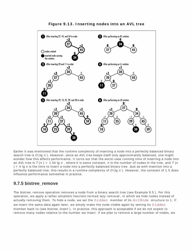
Figure 9.13. Inserting nodes into an AVL tree
Earlier it was mentioned that the runtime complexity of inserting a node into a perfectly balanced binarysearch tree is O (lg n ). However, since an AVL tree keeps itself only approximately balanced, one mightwonder how this affects performance. It turns out that the worst-case running time of inserting a node intoan AVL tree is T (n ) = 1.5k lg n , where k is some constant, n is the number of nodes in the tree, and T (n) = k lg n is the time to insert a node into a perfectly balanced binary tree. Just as with insertion into aperfectly balanced tree, this results in a runtime complexity of O (lg n ). However, the constant of 1.5 doesinfluence performance somewhat in practice.
9.7.5 bistree_remove
The bistree_remove operation removes a node from a binary search tree (see Example 9.5 ). For thisoperation, we apply a rather simplistic heuristic termed lazy removal , in which we hide nodes instead of
actually removing them. To hide a node, we set the hidden member of its AvlNode structure to 1. If
we insert the same data again later, we simply make the node visible again by setting its hiddenmember back to (see bistree_insert ). In practice, this approach is acceptable if we do not expect toremove many nodes relative to the number we insert. If we plan to remove a large number of nodes, we

might consider actually removing the node and adjusting the tree. To locate the node to hide, werecursively call hide until we reach the node we are looking for. Once we hide the node, there is no need to
rebalance the tree because we did not change its structure. Thus, we set balanced to 1.
The analysis of removing a node from an AVL tree is the same as for inserting a node. Thus, the runtimecomplexity of bistree_remove is O (lg n ).
9.7.6 bistree_lookup
The bistree_lookup operation searches for a node within a binary search tree and returns a pointer to the
data member of its AvlNode structure (see Example 9.5 ). The operation works by calling lookup
recursively to descend through the tree until the desired node is found. At each level, we first check if wehave reached the end of a branch. If we reach the end of a branch, the node we are looking for does notexist. Otherwise, we move to either the left or right in the same manner as described for bistree_insert .The recursion terminates once we encounter the desired node, at which point we return 0.
The analysis of searching an AVL tree is the same as for inserting a node. Thus, the runtime complexity ofbistree_lookup is O (lg n ).
9.7.7 bistree_size
This macro evaluates to the size of a set (see Example 9.4 ). It works by accessing the size member of
the BisTree structure.
The runtime complexity of bistree_size is O (1) because accessing a member of a structure is a simple taskthat runs in a constant amount of time.
Example 9.5. Implementation of the Binary Search Tree Abstract Datatype
/****************************************************************************** ** ------------------------------- bistree.c ------------------------------ ** ******************************************************************************/
#include <stdlib.h>#include <string.h>
#include "bistree.h"static void destroy_right(BisTree *tree, BiTreeNode *node);/****************************************************************************** ** ------------------------------ rotate_left ----------------------------- ** ******************************************************************************/
static void rotate_left(BiTreeNode **node) {
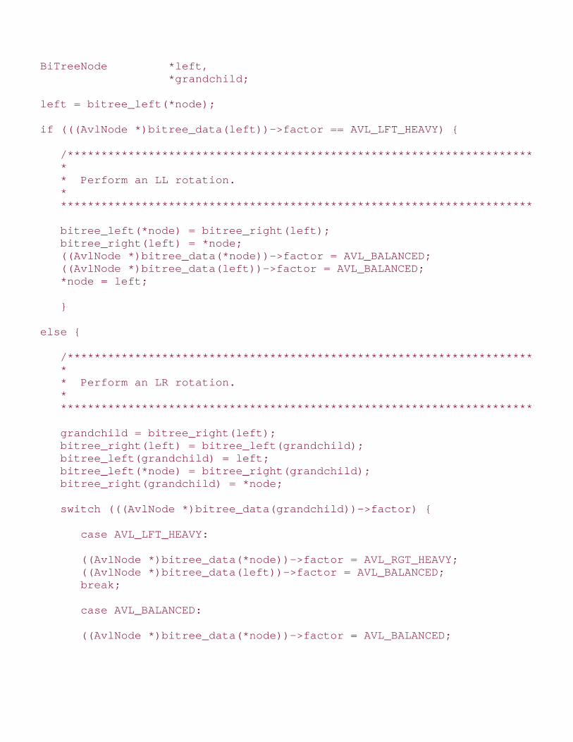
BiTreeNode *left, *grandchild;
left = bitree_left(*node);
if (((AvlNode *)bitree_data(left))->factor == AVL_LFT_HEAVY) {
/************************************************************************** * * * Perform an LL rotation. * * * **************************************************************************/
bitree_left(*node) = bitree_right(left); bitree_right(left) = *node; ((AvlNode *)bitree_data(*node))->factor = AVL_BALANCED; ((AvlNode *)bitree_data(left))->factor = AVL_BALANCED; *node = left;
}
else {
/************************************************************************** * * * Perform an LR rotation. * * * **************************************************************************/
grandchild = bitree_right(left); bitree_right(left) = bitree_left(grandchild); bitree_left(grandchild) = left; bitree_left(*node) = bitree_right(grandchild); bitree_right(grandchild) = *node;
switch (((AvlNode *)bitree_data(grandchild))->factor) {
case AVL_LFT_HEAVY:
((AvlNode *)bitree_data(*node))->factor = AVL_RGT_HEAVY; ((AvlNode *)bitree_data(left))->factor = AVL_BALANCED; break;
case AVL_BALANCED:
((AvlNode *)bitree_data(*node))->factor = AVL_BALANCED;
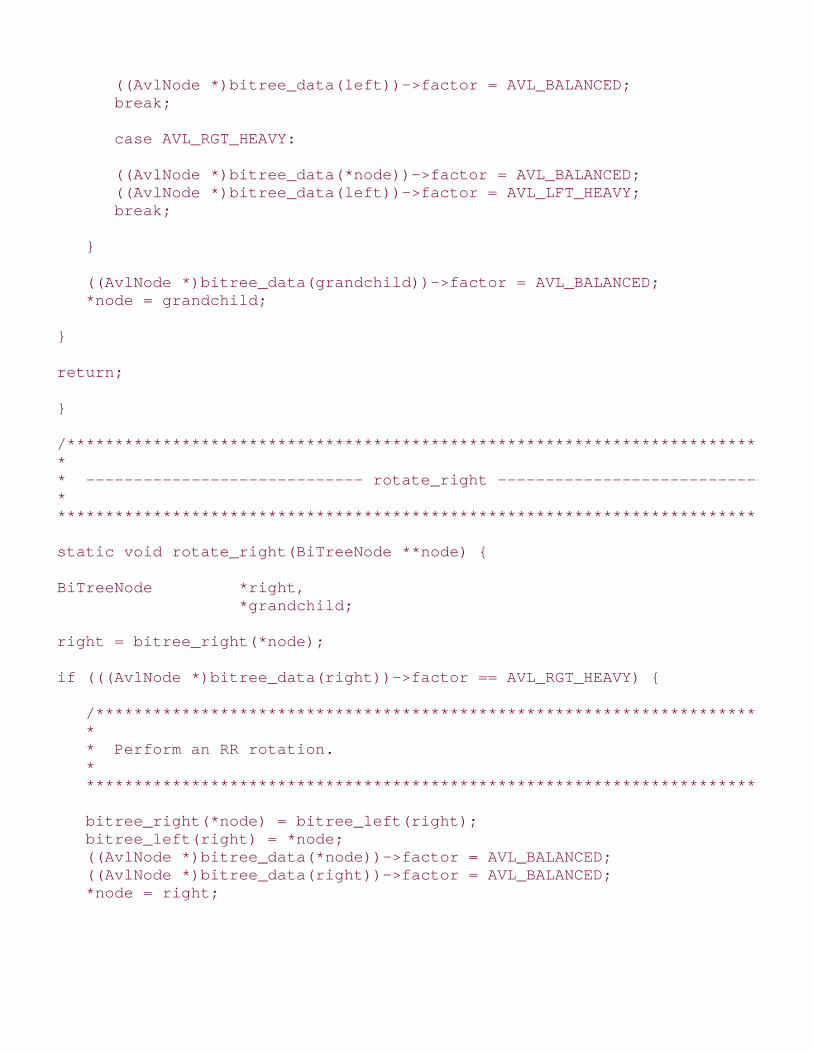
((AvlNode *)bitree_data(left))->factor = AVL_BALANCED; break;
case AVL_RGT_HEAVY:
((AvlNode *)bitree_data(*node))->factor = AVL_BALANCED; ((AvlNode *)bitree_data(left))->factor = AVL_LFT_HEAVY; break;
}
((AvlNode *)bitree_data(grandchild))->factor = AVL_BALANCED; *node = grandchild;
}
return;
}
/****************************************************************************** ** ----------------------------- rotate_right ----------------------------- ** ******************************************************************************/
static void rotate_right(BiTreeNode **node) {
BiTreeNode *right, *grandchild;
right = bitree_right(*node);
if (((AvlNode *)bitree_data(right))->factor == AVL_RGT_HEAVY) {
/************************************************************************** * * * Perform an RR rotation. * * * **************************************************************************/
bitree_right(*node) = bitree_left(right); bitree_left(right) = *node; ((AvlNode *)bitree_data(*node))->factor = AVL_BALANCED; ((AvlNode *)bitree_data(right))->factor = AVL_BALANCED; *node = right;
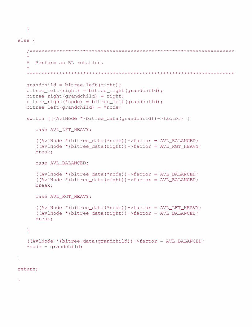
}
else {
/************************************************************************** * * * Perform an RL rotation. * * * **************************************************************************/
grandchild = bitree_left(right); bitree_left(right) = bitree_right(grandchild); bitree_right(grandchild) = right; bitree_right(*node) = bitree_left(grandchild); bitree_left(grandchild) = *node;
switch (((AvlNode *)bitree_data(grandchild))->factor) {
case AVL_LFT_HEAVY:
((AvlNode *)bitree_data(*node))->factor = AVL_BALANCED; ((AvlNode *)bitree_data(right))->factor = AVL_RGT_HEAVY; break;
case AVL_BALANCED:
((AvlNode *)bitree_data(*node))->factor = AVL_BALANCED; ((AvlNode *)bitree_data(right))->factor = AVL_BALANCED; break;
case AVL_RGT_HEAVY:
((AvlNode *)bitree_data(*node))->factor = AVL_LFT_HEAVY; ((AvlNode *)bitree_data(right))->factor = AVL_BALANCED; break;
}
((AvlNode *)bitree_data(grandchild))->factor = AVL_BALANCED; *node = grandchild;
}
return;
}

/****************************************************************************** ** ----------------------------- destroy_left ----------------------------- ** ******************************************************************************/
static void destroy_left(BisTree *tree, BiTreeNode *node) {
BiTreeNode **position;
/****************************************************************************** ** Do not allow destruction of an empty tree. ** ******************************************************************************/
if (bitree_size(tree) == 0) return;
/****************************************************************************** ** Determine where to destroy nodes. * * ******************************************************************************/
if (node == NULL) position = &tree->root;else position = &node->left;
/****************************************************************************** ** Destroy the nodes. ** ******************************************************************************/
if (*position != NULL) {
destroy_left(tree, *position); destroy_right(tree, *position);
if (tree->destroy != NULL) {
/*********************************************************************** * *

* Call a user-defined function to free dynamically allocated data. * * * ***********************************************************************/
tree->destroy(((AvlNode *)(*position)->data)->data);
}
/************************************************************************** * * * Free the AVL data in the node, then free the node itself. * * * **************************************************************************/
free((*position)->data); free(*position); *position = NULL;
/************************************************************************** * * * Adjust the size of the tree to account for the destroyed node. * * * **************************************************************************/
tree->size--;
}
return;
}
/****************************************************************************** ** ----------------------------- destroy_right ---------------------------- ** ******************************************************************************/
static void destroy_right(BisTree *tree, BiTreeNode *node) {
BiTreeNode **position;
/****************************************************************************** ** Do not allow destruction of an empty tree. ** *

*****************************************************************************/
if (bitree_size(tree) == 0) return;
/****************************************************************************** ** Determine where to destroy nodes. ** ******************************************************************************/
if (node == NULL) position = &tree->root;else position = &node->right;
/****************************************************************************** ** Destroy the nodes. ** ******************************************************************************/
if (*position != NULL) {
destroy_left(tree, *position); destroy_right(tree, *position);
if (tree->destroy != NULL) {
/*********************************************************************** * * * Call a user-defined function to free dynamically allocated data. * * * ***********************************************************************/
tree->destroy(((AvlNode *)(*position)->data)->data);
}
/************************************************************************** * * * Free the AVL data in the node, then free the node itself. * * * **************************************************************************/
free((*position)->data);

free(*position); *position = NULL;
/************************************************************************** * * * Adjust the size of the tree to account for the destroyed node. * * * **************************************************************************/
tree->size--;
}
return;
}
/****************************************************************************** ** -------------------------------- insert -------------------------------- ** ******************************************************************************/
static int insert(BisTree *tree, BiTreeNode **node, const void *data, int *balanced) {
AvlNode *avl_data;
int cmpval, retval;
/****************************************************************************** ** Insert the data into the tree. ** ******************************************************************************/
if (bitree_is_eob(*node)) {
/************************************************************************** * * * Handle insertion into an empty tree. * * * **************************************************************************/
if ((avl_data = (AvlNode *)malloc(sizeof(AvlNode))) == NULL)

return -1;
avl_data->factor = AVL_BALANCED; avl_data->hidden = 0; avl_data->data = (void *)data;
return bitree_ins_left(tree, *node, avl_data);
}
else {
/************************************************************************** * * * Handle insertion into a tree that is not empty. * * * **************************************************************************/
cmpval = tree->compare(data, ((AvlNode *)bitree_data(*node))->data);
if (cmpval < 0) {
/*********************************************************************** * * * Move to the left. * * * ***********************************************************************/
if (bitree_is_eob(bitree_left(*node))) {
if ((avl_data = (AvlNode *)malloc(sizeof(AvlNode))) == NULL) return -1;
avl_data->factor = AVL_BALANCED; avl_data->hidden = 0; avl_data->data = (void *)data;
if (bitree_ins_left(tree, *node, avl_data) != 0) return -1;
*balanced = 0;
}
else {

if ((retval = insert(tree, &bitree_left(*node), data, balanced)) != 0) {
return retval;
}
}
/*********************************************************************** * * * Ensure that the tree remains balanced. * * * ***********************************************************************/
if (!(*balanced)) {
switch (((AvlNode *)bitree_data(*node))->factor) {
case AVL_LFT_HEAVY:
rotate_left(node); *balanced = 1; break;
case AVL_BALANCED:
((AvlNode *)bitree_data(*node))->factor = AVL_LFT_HEAVY; break;
case AVL_RGT_HEAVY:
((AvlNode *)bitree_data(*node))->factor = AVL_BALANCED; *balanced = 1;
}
}
} /* if (cmpval < 0) */
else if (cmpval > 0) {
/*********************************************************************** * * * Move to the right. *

* * ***********************************************************************/
if (bitree_is_eob(bitree_right(*node))) {
if ((avl_data = (AvlNode *)malloc(sizeof(AvlNode))) == NULL) return -1;
avl_data->factor = AVL_BALANCED; avl_data->hidden = 0; avl_data->data = (void *)data;
if (bitree_ins_right(tree, *node, avl_data) != 0) return -1;
*balanced = 0;
}
else {
if ((retval = insert(tree, &bitree_right(*node), data, balanced)) != 0) {
return retval;
}
}
/*********************************************************************** * * * Ensure that the tree remains balanced. * * * ***********************************************************************/
if (!(*balanced)) {
switch (((AvlNode *)bitree_data(*node))->factor) {
case AVL_LFT_HEAVY:
((AvlNode *)bitree_data(*node))->factor = AVL_BALANCED; *balanced = 1; break;

case AVL_BALANCED:
((AvlNode *)bitree_data(*node))->factor = AVL_RGT_HEAVY; break;
case AVL_RGT_HEAVY:
rotate_right(node); *balanced = 1;
}
}
} /* if (cmpval > 0) */
else {
/************************************************************************* * * * Handle finding a copy of the data. * * * *************************************************************************/
if (!((AvlNode *)bitree_data(*node))->hidden) {
/******************************************************************** * * * Do nothing since the data is in the tree and not hidden. * * *
return 1;
}
else {
/******************************************************************** * * * Insert the new data and mark it as not hidden. * * * ********************************************************************/
if (tree->destroy != NULL) {
/*****************************************************************

* * * Destroy the hidden data since it is being replaced. * * * *****************************************************************/
tree->destroy(((AvlNode *)bitree_data(*node))->data);
}
((AvlNode *)bitree_data(*node))->data = (void *)data; ((AvlNode *)bitree_data(*node))->hidden = 0;
/******************************************************************** * * * Do not rebalance because the tree structure is unchanged. * * * ********************************************************************/
*balanced = 1;
}
}
}
return 0;
}
/***************************************************************************** ** --------------------------------- hide -------------------------------- ** *****************************************************************************/
static int hide(BisTree *tree, BiTreeNode *node, const void *data) {
int cmpval, retval;
if (bitree_is_eob(node)) {
/************************************************************************** * * * Return that the data was not found. *

* * **************************************************************************/
return -1;
}
cmpval = tree->compare(data, ((AvlNode *)bitree_data(node))->data);
if (cmpval < 0) {
/************************************************************************** * * * Move to the left. * * * **************************************************************************/
retval = hide(tree, bitree_left(node), data);
}
else if (cmpval > 0) {
/************************************************************************** * * * Move to the right. * * * **************************************************************************/
retval = hide(tree, bitree_right(node), data);
}
else {
/************************************************************************** * * * Mark the node as hidden. * * * **************************************************************************/
((AvlNode *)bitree_data(node))->hidden = 1; retval = 0;
}

return retval;
}/***************************************************************************** ** -------------------------------- lookup ------------------------------- ** *****************************************************************************/
static int lookup(BisTree *tree, BiTreeNode *node, void **data) {
int cmpval, retval;
if (bitree_is_eob(node)) {
/************************************************************************** * * * Return that the data was not found. * * * **************************************************************************/
return -1;
}
cmpval = tree->compare(*data, ((AvlNode *)bitree_data(node))->data);
if (cmpval < 0) {
/************************************************************************** * * * Move to the left. *
retval = lookup(tree, bitree_left(node), data);
}
else if (cmpval > 0) {
/************************************************************************** * * * Move to the right. * * * **************************************************************************/

retval = lookup(tree, bitree_right(node), data);
}
else {
if (!((AvlNode *)bitree_data(node))->hidden) {
/*********************************************************************** * * * Pass back the data from the tree. * * * ***********************************************************************/
*data = ((AvlNode *)bitree_data(node))->data; retval = 0;
}
else {
/*********************************************************************** * * * Return that the data was not found. * * * ***********************************************************************/
return -1;
}
}
return retval;
}
/***************************************************************************** ** ----------------------------- bistree_init ---------------------------- ** *****************************************************************************/
void bistree_init(BisTree *tree, int (*compare)(const void *key1, const void *key2), void (*destroy)(void *data)) {

/***************************************************************************** ** Initialize the tree. ** *****************************************************************************/
bitree_init(tree, destroy);tree->compare = compare;
return;
}
/***************************************************************************** ** ---------------------------- bistree_destroy -------------------------- ** *****************************************************************************/
void bistree_destroy(BisTree *tree) {
/***************************************************************************** ** Destroy all nodes in the tree. ** *****************************************************************************/
destroy_left(tree, NULL);
/***************************************************************************** ** No operations are allowed now, but clear the structure as a precaution. ** *****************************************************************************/
memset(tree, 0, sizeof(BisTree));
return;
}
/***************************************************************************** ** ---------------------------- bistree_insert --------------------------- ** *****************************************************************************/

int bistree_insert(BisTree *tree, const void *data) {
int balanced = 0;
return insert(tree, &bitree_root(tree), data, &balanced);
}
/***************************************************************************** ** ---------------------------- bistree_remove --------------------------- ** *****************************************************************************/
int bistree_remove(BisTree *tree, const void *data) {
return hide(tree, bitree_root(tree), data);
}
/***************************************************************************** ** ---------------------------- bistree_lookup --------------------------- ** *****************************************************************************/
int bistree_lookup(BisTree *tree, void **data) {
return lookup(tree, bitree_root(tree), data);
}
Top

Mastering Algorithms with CBy Kyle Loudon
Slots : 1
Table of Contents
Chapter 9. Trees
Content
9.8 Questions and Answers
Q: Akin to doubly-linked lists, some trees maintain pointers from child nodes back to their parents inaddition to the normal pointers from parents to their children. Some trees maintain pointers betweensibling nodes as well. Why might we do this?
A: In general, maintaining additional pointers gives us greater flexibility in how we traverse a tree.For example, maintaining pointers from a parent to its children and from a child to its parent lets usmove both up and down through a tree. Maintaining pointers between siblings gives us an easy wayto traverse through a node's children without accessing the parent. One benefit of linked siblings isfound in B +-trees, a type of balanced search tree in which pointers are used to link leaf nodestogether. By linking leaf nodes, we effectively form a linked list at the bottom of the tree. Thisprovides an efficient means of looking up a particular key and then retrieving others that eitherprecede or follow it in a sequence. Database systems do this to support efficient random andsequential access simultaneously. Of course, the disadvantage is some overhead and complication inmanaging the sibling pointers as children are inserted and removed.
Q: Recall that the example on expression processing used a linked list to return the appropriateordering of the nodes to the caller. This example illustrates two data structures pointing to the samedata. What precautions would we need to take in destroying each instance of these datatypes?
A: All of the data structures presented in this book follow the convention that only a pointer ismaintained to the data inserted into the data structure. Therefore, it is the responsibility of the callerto manage the storage associated with the data itself. In the case of a binary tree and a linked listpointing to the same physical data in memory, it is important that we pass a function to free the dataonly to one of the initialization operations. The other operation must set destroy to NULL. Ofcourse, this approach assumes that the data being shared was dynamically allocated in the firstplace. If the data structures point to data that was not dynamically allocated, destroy should beset to NULL in both initialization operations since there is nothing to free.
Q: In bitree_rem_left and bitree_rem_right, why was a postorder traversal used to remove theappropriate subtree? Could a preorder or inorder traversal have been used instead?
A: It is essential to use a postorder traversal here because a subtree must be removed in its entiretybefore removing its parent. A preorder traversal ends up removing the parent first, thus freeing theparent and making it impossible to access its children. An inorder traversal also does not workbecause we still end up removing the parent before its right subtree.

Q: How do we find the smallest node in a binary search tree? What is the runtime complexity to dothis in both an unbalanced and balanced binary search tree, in the worst case? How do we find thelargest node in a binary search tree? What are the runtime complexities for this?
A: The smallest node in a binary search tree is the node that is the furthest to the left. To locate thisnode, we descend through the tree by following left pointers until reaching the end of the branch. Inan unbalanced binary search tree, this requires O (n) time in the worst case, where n is the numberof nodes in the tree. This occurs when the tree consists of a single branch to the left, for example.However, if we keep the tree balanced, no branch will be longer than lg n nodes. Thus, the runtimecomplexity of searching for the smallest node in this case is O (lg n). Finding the largest node is asimilar process, except that the largest node is the one that is the furthest to the right in the tree.The runtime complexities for this are the same as for locating the smallest node. If we are interestedonly in determining the smallest (or largest) element in a set of data repeatedly, we use a priorityqueue (see Chapter 10).
Q: When might we choose to make use of a tree with a relatively large branching factor, instead of abinary tree, for example?
A: Larger branching factors keep a tree shorter for a given number of nodes, provided the treeremains relatively balanced. Therefore, a large branching factor is desirable when an application isparticularly sensitive to the height of the tree. Search trees are a good example, although typicallythe difference in performance attributed to larger branching factors is not that significant when thetree resides in memory. This is one reason that binary trees are most common for searching inmemory. However, when searching in the considerably slower world of secondary storage, a largerbranching factor can make a substantial difference. In this situation, typically some type of B-tree isused (see the related topics at the end of the chapter).
Q: In a binary search tree, the successor of some node x is the next largest node after x. Forexample, in a binary search tree containing the keys 24, 39, 41, 55, 87, 92, the successor of 41 is55. How do we find the successor of a node in a binary search tree? What is the runtime complexityof this operation?
A: To determine the successor of some node x in a binary search tree, first we locate x. Next, wefollow its right pointer, and then from this node, follow as many left pointers as possible until the endof the branch is reached. The node at the end of this branch is the successor of x. The runtimecomplexity of locating either x or its successor is O (lg n).
Q: In a binary search tree, recall that to insert a node, we trace a specific path to determine theproper point at which to actually insert it. As more and more nodes are inserted into a tree, certainareas within the tree become restricted to certain values. Ultimately, this is why a tree falls out ofbalance and rotations are performed. In the binary search tree of Figure 9.14, what are the possiblevalues for a node inserted at x?
A: In Figure 9.14, any node we insert at x must contain a value greater than 44 and less than 49because any node to the left of 49 must be less than 49. On the other hand, the only way for a nodeto end up in the right subtree of 44 is to be greater than 44.
Figure 9.14. A balanced binary search tree

Top

Mastering Algorithms with CBy Kyle Loudon
Slots : 1
Table of Contents
Chapter 9. Trees
Content
9.9 Related Topics
k-ary trees
Trees that have a branching factor of k. Branching factors of more than two children per nodeare useful when modeling certain situations, such as the 1-to-n relationship of a parent windowand its children in a graphical windowing system, or a directory structure in a file system.
Red-black trees
Binary search trees that keep themselves approximately balanced by maintaining a color witheach node, which is either red or black. By enforcing a policy about how nodes can be coloredalong a branch, red-black trees ensure that no branch will ever become more than twice aslong as any other. The worst-case running time of searching a red-black tree is T (n) = 2k lg n,where n is the number of nodes in the tree, k is some constant, and T (n) = k lg n is the timeto search a perfectly balanced tree.
Tries
Search trees used primarily to search sets of variable-length strings. Conceptually, the nodesat each level in a trie (pronounced "try") represent all characters found at a particular positionin the strings being searched. For example, the nodes immediately below the root represent allpossible characters in position 1 of the strings, the next level represents all possible charactersin position 2, and so forth. Thus, to look up a string, we start at the root and at each levelfollow the pointer to the node containing the next character in the string we are searching for.This procedure results in search times that are dependent on the size of the search stringrather than the number of strings being searched.
B-trees, B+-trees, and B*-trees
Search trees typically used by database systems to improve the performance of accessing datastored on secondary storage devices. Generally, node size is optimized to coincide with theblock size of the secondary storage device. All types of B-trees are balanced and typically havea large branching factor. This reduces the number of levels that must be traversed to get at aparticular record, thus saving costly accesses to I/O.
Top

Mastering Algorithms with CBy Kyle Loudon
Slots : 1
Table of Contents
Part II: Data Structures
Content
Chapter 10. Heaps and Priority QueuesMany problems rely on being able to determine quickly the largest or smallest element from a setthat is undergoing frequent insertions and deletions. One way to approach this problem is to keep aset sorted. This way, the largest or smallest element, depending on whether we sort the data inascending or descending order, is always the one at the beginning of the set. However, sorting a setover and over again is costly. In addition, because it is not our goal to keep every element in order,we end up doing more work than we really need to. To quickly determine only the largest or smallestelement, we need only keep this element where we can find it. Heaps and priority queues let us dothis in an efficient way.
This chapter covers:
Heaps
Trees organized so that we can determine the node with the largest value quickly. The cost topreserve this property is less than that of keeping the data sorted. We can also organize aheap so that we can determine the smallest value just as easily.
Priority queues
Data structures naturally derived from heaps. In a priority queue, data is organized in a heapso that we can determine the node with the next highest priority quickly. The "priority" of anelement can mean different things in different problems.
Some applications of heaps and priority queues are:
Sorting
Specifically, an algorithm called heapsort. In heapsort, the data to be sorted begins in a heap.Nodes are extracted from the heap one at a time and placed at the end of a sorted set. Aseach node is extracted, the next node for the sorted set percolates to the top of the heap.Heapsort has the same runtime complexity as quicksort (see Chapter 12 ), but a goodimplementation of quicksort usually beats it by a small constant factor in practice.
Task scheduling
For example, that performed by operating systems to determine which process is next to runon a CPU. Operating systems continually change the priorities of processes. A priority queue isan efficient way to ensure that the highest-priority process is next to get the CPU.

Parcel sorting (illustrated in this chapter)
A process used by delivery companies to prioritize the routing of parcels. As parcels arescanned, high priorities are assigned to those requiring urgent delivery. Parcels that are lessurgent are assigned lower priorities. A computer system might use a priority queue as anefficient means of ensuring that the highest priority parcels move through the system thefastest.
Huffman coding
A method of data compression that uses a Huffman tree to assign codes to symbols in the data(see Chapter 14). Frequently occurring symbols are assigned short codes, whereas symbolsoccuring less frequently are assigned longer ones. The Huffman tree is built by merging smallerbinary trees two by two. The two trees merged at each step are extracted from a priorityqueue because we merge the two with the smallest key values.
Load balancing
Often usage statistics are maintained about a number of servers handling similar tasks. Asconnection requests arrive, a priority queue can be used to determine which server is best ableto accommodate a new request.
Top

Mastering Algorithms with CBy Kyle Loudon
Slots : 1
Table of Contents
Chapter 10. Heaps and Priority Queues
Content
10.1 Description of Heaps
A heap is a tree, usually a binary tree, in which each child node has a smaller value than its parent.Thus, the root node is the largest node in the tree. We may also choose to orient a heap so that eachchild node has a larger value than its parent. In this case, the root node is the smallest node. Treeslike these are partially ordered because, although the nodes along every branch have a specific orderto them, the nodes at one level are not necessarily ordered with respect to the nodes at another. Aheap in which each child is smaller than its parent is top-heavy. This is because the largest node ison top (see Figure 10.1). A heap in which each child is larger than its parent is bottom-heavy .
Heaps are left-balanced (see Chapter 9), so as nodes are added, the tree grows level by level fromleft to right. A particularly good way to represent left-balanced binary trees, and therefore heaps, isto store nodes contiguously in an array in the order we would encounter them in a level traversal(see Chapter 9). Assuming a zero-indexed array, this means that the parent of each node at someposition i in the array is located at position (i - 1)/2 , where means to ignore the fractionalpart of (i - 1)/2. The left and right children of a node are located at positions 2i + 1 and 2i + 2. Thisorganization is especially important for heaps because it allows us to locate a heap's last nodequickly: the last node is the rightmost node at the deepest level. This is important in implementingcertain heap operations.
Figure 10.1. A top-heavy heap (a) conceptually and (b) represented in anarray

Top

Mastering Algorithms with CBy Kyle LoudonSlots : 1Table of ContentsChapter 10. Heaps and Priority Queues
Content
10.2 Interface for Heapsheap_init
void heap_init(Heap *heap, int (*compare)(const void *key1, const void *key2) void (*destroy)(void *data));
Return Value
None.
Description
Initializes the heap specified by heap . This operation must be called for a heap before the heap can be
used with any other operation. The compare argument is a function used by various heap operations to
compare nodes when fixing the heap. This function should return 1 if key1 > key2 , if key1 = key2 ,
and -1 if key1 < key2 for a top-heavy heap. For a bottom-heavy heap, compare should reverse the
cases that return 1 and -1. The destroy argument provides a way to free dynamically allocated data
when heap_destroy is called. For example, if the heap contains data dynamically allocated using malloc ,
destroy should be set to free to free the data as the heap is destroyed. For structured data containing
several dynamically allocated members, destroy should be set to a user-defined function that calls free
for each dynamically allocated member as well as for the structure itself. For a heap containing data that
should not be freed, destroy should be set to NULL.
Complexity
O (1)
heap_destroy

void heap_destroy(Heap *heap);
Return Value
None.
Description
Destroys the heap specified by heap . No other operations are permitted after calling heap_destroy unless
heap_init is called again. The heap_destroy operation removes all nodes from a heap and calls the function
passed as destroy to heap_init once for each node as it is removed, provided destroy was not set to
NULL.
Complexity
O (n ), where n is the number of nodes in the heap.
heap_insert
int heap_insert(Heap *heap, const void *data);
Return Value
0if inserting the node is successful, or -1 otherwise.
Description
Inserts a node into the heap specified by heap . The new node contains a pointer to data , so the
memory referenced by data should remain valid as long as the node remains in the heap. It is the
responsibility of the caller to manage the storage associated with data .
Complexity
O (lg n ), where n is the number of nodes in the heap.
heap_extract
int heap_extract(Heap *heap, void **data);
Return Value
0if extracting the node is successful, or -1 otherwise.

Description
Extracts the node at the top of the heap specified by heap . Upon return, data points to the data stored
in the node that was extracted. It is the responsibility of the caller to manage the storage associated withthe data.
Complexity
O (lg n ), where n is the number of nodes in the heap.
heap_size
int heap_size(const Heap *heap);
Return Value
Number of nodes in the heap.
Description
Macro that evaluates to the number of nodes in the heap specified by heap .
Complexity
O (1)
Top

Mastering Algorithms with CBy Kyle LoudonSlots : 1Table of ContentsChapter 10. Heaps and Priority Queues
Content
10.3 Implementation and Analysis of Heaps
The heap implemented here is a binary tree whose nodes are arranged hierarchically in an array. The
structure Heap is the heap data structure (see Example 10.1 ). This structure consists of four members:
size is the number of nodes in the heap, compare and destroy are members used to encapsulate
the functions passed to heap_init , and tree is the array of nodes in the heap.
Example 10.1. Header for the Heap Abstract Datatype
/****************************************************************************** ** -------------------------------- heap.h -------------------------------- ** ******************************************************************************/
#ifndef HEAP_H#define HEAP_H
/****************************************************************************** ** Define a structure for heaps. ** ******************************************************************************/
typedef struct Heap_ {
int size;
int (*compare)(const void *key1, const void *key2);

void (*destroy)(void *data);
void **tree;
} Heap;
/****************************************************************************** ** --------------------------- Public Interface --------------------------- ** ******************************************************************************/
void heap_init(Heap *heap, int (*compare)(const void *key1, const void *key2), void (*destroy)(void *data));
void heap_destroy(Heap *heap);
int heap_insert(Heap *heap, const void *data);
int heap_extract(Heap *heap, void **data);
#define heap_size(heap) ((heap)->size)
#endif
10.3.1 heap_init
The heap_init operation initializes a heap so that it can be used in other operations (see Example 10.2 ).
Initializing a heap is a simple operation in which we set the size member of the heap to 0, the destroymember to destroy , and the tree pointer to NULL.
The runtime complexity of heap_init is O (1) because all of the steps in initializing a heap run in a constantamount of time.
10.3.2 heap_destroy
The heap_destroy operation destroys a heap (see Example 10.2 ). Primarily this means removing all nodes
from the heap. The function passed as destroy to heap_init is called once for each node as it is
removed, provided destroy was not set to NULL.
The runtime complexity of heap_destroy is O (n ), where n is the number of nodes in the heap. This is
because we must traverse all nodes in the heap in order to free the data they contain. If destroy is
NULL, heap_destroy runs in O (1) time.
10.3.3 heap_insert

The heap_insert operation inserts a node into a heap (see Example 10.2 ). The call sets the new node topoint to the data passed by the caller. To begin, we reallocate storage to enable the tree to accommodatethe new node. The actual process of inserting the new node initially places it into the last position in thearray. When this causes the heap property to be violated, we must reheapify the tree (see Figure 10.2 ).
Figure 10.2. Inserting 24 into a top-heavy heap
To reheapify a tree after inserting a node, we need only consider the branch in which the new node hasbeen inserted, since the tree was a heap to begin with. Starting at the new node, we move up the tree levelby level, comparing each child with its parent. At each level, if a parent and child are in the wrong order,

we swap their contents. This process continues until we reach a level at which no swap is required, or we
reach the top of the tree. Last, we update the size of the heap by incrementing the size member of the
heap data structure.
The runtime complexity of heap_insert is O (lg n ), where n is the number of nodes in the tree. This isbecause heapification requires moving the contents of the new node from the lowest level of the tree to thetop in the worst case, a traversal of lg n levels. All other parts of the operation run in a constant amount oftime.
10.3.4 heap_extract
The heap_extract operation extracts the node at the top of a heap (see Example 10.2 ). To begin, we set
data to point to the data stored in the node being extracted. Next, we save the contents of the last node,
reallocate a smaller amount of storage for the tree, and decrease the tree size by 1. After we are certainthis has succeeded, we copy the contents of the saved last node to the root node. When this causes theheap property to be violated, we must reheapify the tree (see Figure 10.3 ).
To reheapify a tree after extracting a node, we start at the root node and move down the tree level bylevel, comparing each node with its two children. At each level, if a parent and its children are in the wrongorder, we swap their contents and move to the child that was the most out of order. This process continuesuntil we reach a level at which no swap is required, or we reach a leaf node. Last, we update the size of the
heap by decreasing the size member of the heap data structure by 1.
The runtime complexity of heap_extract is O (lg n ), where n is the number of nodes in the tree. This isbecause heapification requires moving the contents of the root node from the top of the tree to a leaf nodein the worst case, a traversal of lg n levels. All other parts of the operation run in a constant amount oftime.
10.3.5 heap_size
This macro evaluates to the number of nodes in a heap (see Example 10.1 ). It works by accessing the
size member of the Heap structure.
Figure 10.3. Extracting 25 from a top-heavy heap
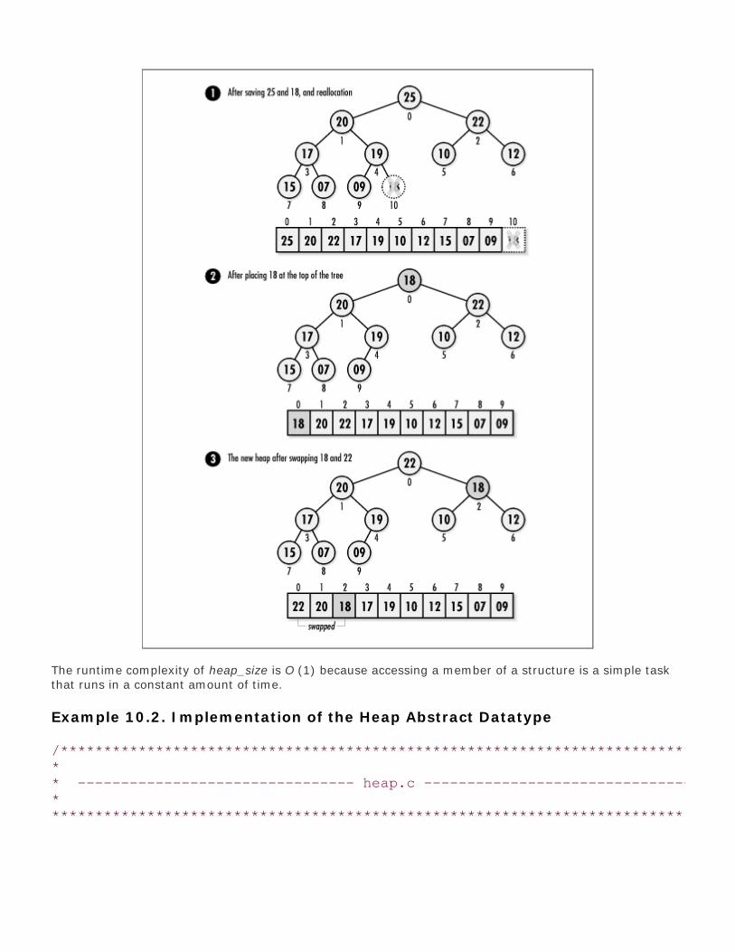
The runtime complexity of heap_size is O (1) because accessing a member of a structure is a simple taskthat runs in a constant amount of time.
Example 10.2. Implementation of the Heap Abstract Datatype
/****************************************************************************** ** -------------------------------- heap.c -------------------------------- ** ******************************************************************************/

#include <stdlib.h>#include <string.h>
#include "heap.h"
/****************************************************************************** ** Define private macros used by the heap implementation. ** ******************************************************************************/
#define heap_parent(npos) ((int)(((npos) - 1) / 2))
#define heap_left(npos) (((npos) * 2) + 1)
#define heap_right(npos) (((npos) * 2) + 2)
/****************************************************************************** ** ------------------------------- heap_init ------------------------------ ** ******************************************************************************/
void heap_init(Heap *heap, int (*compare)(const void *key1, const void *key2), void (*destroy)(void *data)) {
/****************************************************************************** ** Initialize the heap. ** ******************************************************************************/
heap->size = 0;heap->compare = compare;heap->destroy = destroy;heap->tree = NULL;
return;
}
/****************************************************************************** ** ----------------------------- heap_destroy ----------------------------- ** *

*****************************************************************************/
void heap_destroy(Heap *heap) {
int i;
/****************************************************************************** ** Remove all the nodes from the heap. ** ******************************************************************************/
if (heap->destroy != NULL) {
for (i = 0; i < heap_size(heap); i++) {
/*********************************************************************** * * * Call a user-defined function to free dynamically allocated data. * * * ***********************************************************************/
heap->destroy(heap->tree[i]);
}
}
/****************************************************************************** ** Free the storage allocated for the heap. ** ******************************************************************************/
free(heap->tree);
/****************************************************************************** ** No operations are allowed now, but clear the structure as a precaution. ** ******************************************************************************/
memset(heap, 0, sizeof(Heap));
return;
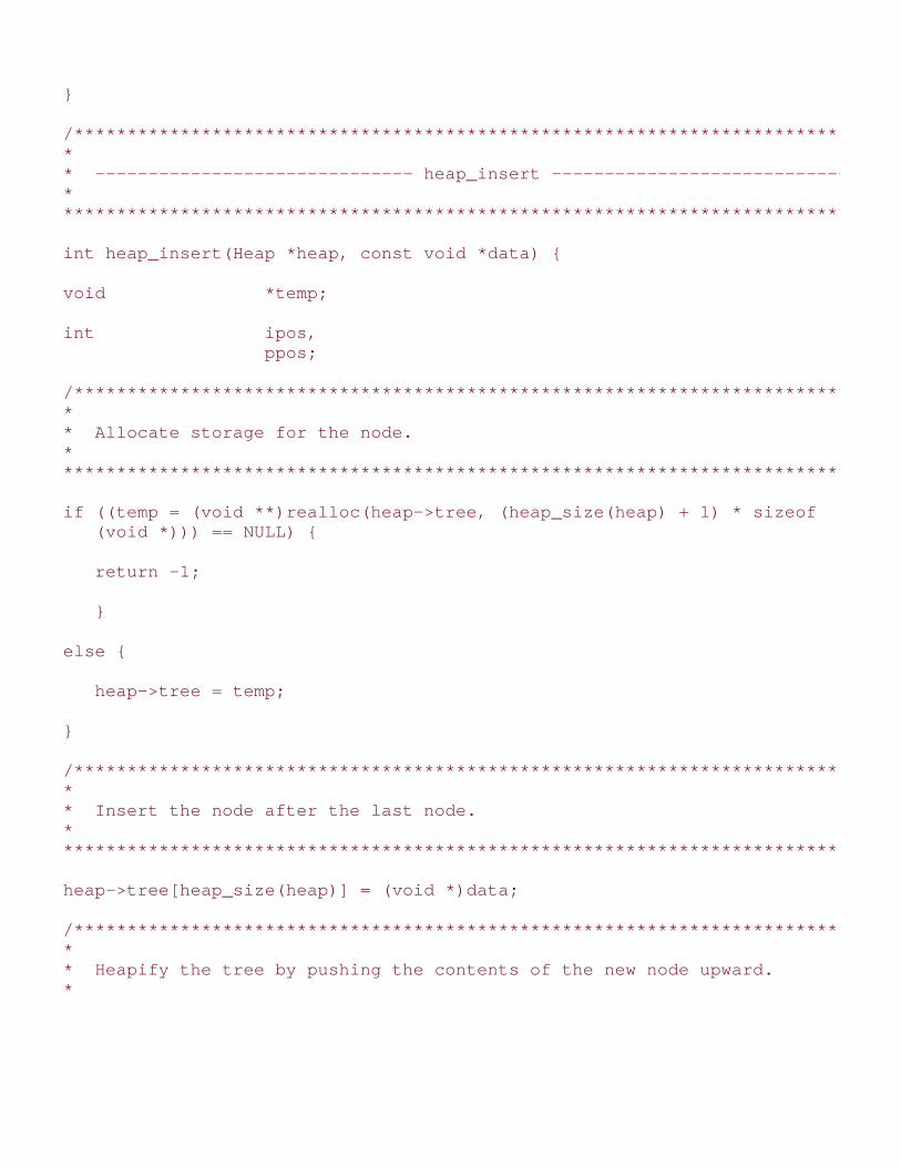
}
/****************************************************************************** ** ------------------------------ heap_insert ----------------------------- ** ******************************************************************************/
int heap_insert(Heap *heap, const void *data) {
void *temp;
int ipos, ppos;
/****************************************************************************** ** Allocate storage for the node. ** ******************************************************************************/
if ((temp = (void **)realloc(heap->tree, (heap_size(heap) + 1) * sizeof (void *))) == NULL) {
return -1;
}
else {
heap->tree = temp;
}
/****************************************************************************** ** Insert the node after the last node. ** ******************************************************************************/
heap->tree[heap_size(heap)] = (void *)data;
/****************************************************************************** ** Heapify the tree by pushing the contents of the new node upward. ** *

*****************************************************************************/
ipos = heap_size(heap);ppos = heap_parent(ipos);
while (ipos > 0 && heap->compare(heap->tree[ppos], heap->tree[ipos]) < 0) {
/************************************************************************** * * * Swap the contents of the current node and its parent. * * * **************************************************************************/
temp = heap->tree[ppos]; heap->tree[ppos] = heap->tree[ipos]; heap->tree[ipos] = temp;
/************************************************************************** * * * Move up one level in the tree to continue heapifying. * * * **************************************************************************/
ipos = ppos; ppos = heap_parent(ipos);
}
/****************************************************************************** ** Adjust the size of the heap to account for the inserted node. ** ******************************************************************************/
heap->size++;
return 0;
}
/****************************************************************************** ** ----------------------------- heap_extract ----------------------------- ** ******************************************************************************/

int heap_extract(Heap *heap, void **data) {
void *save, *temp;
int ipos, lpos, rpos, mpos;
/****************************************************************************** ** Do not allow extraction from an empty heap. ** ******************************************************************************/
if (heap_size(heap) == 0) return -1;
/****************************************************************************** ** Extract the node at the top of the heap. ** ******************************************************************************/
*data = heap->tree[0];
/****************************************************************************** ** Adjust the storage used by the heap. ** ******************************************************************************/
save = heap->tree[heap_size(heap) - 1];
if (heap_size(heap) - 1 > 0) {
if ((temp = (void **)realloc(heap->tree, (heap_size(heap) - 1) * sizeof (void *))) == NULL) {
return -1;
}
else {

heap->tree = temp;
}
/************************************************************************** * * * Adjust the size of the heap to account for the extracted node. * * * **************************************************************************/
heap->size--;
}
else {
/************************************************************************** * * * Manage the heap when extracting the last node. * * * **************************************************************************/
free(heap->tree); heap->tree = NULL; heap->size = 0; return 0;
}
/****************************************************************************** ** Copy the last node to the top. ** ******************************************************************************/
heap->tree[0] = save;
/****************************************************************************** ** Heapify the tree by pushing the contents of the new top downward. ** ******************************************************************************/
ipos = 0;lpos = heap_left(ipos);rpos = heap_right(ipos);

while (1) {
/************************************************************************** * * * Select the child to swap with the current node. * * * **************************************************************************/
lpos = heap_left(ipos); rpos = heap_right(ipos);
if (lpos < heap_size(heap) && heap->compare(heap->tree[lpos], heap-> tree[ipos]) > 0) {
mpos = lpos;
}
else {
mpos = ipos;
}
if (rpos < heap_size(heap) && heap->compare(heap->tree[rpos], heap-> tree[mpos]) > 0) {
mpos = rpos;
}
/************************************************************************** * * * When mpos is ipos, the heap property has been restored. * * * **************************************************************************/
if (mpos == ipos) {
break;
}
else {
/***********************************************************************

* * * Swap the contents of the current node and the selected child. * * * ***********************************************************************/
temp = heap->tree[mpos]; heap->tree[mpos] = heap->tree[ipos]; heap->tree[ipos] = temp;
/*********************************************************************** * * * Move down one level in the tree to continue heapifying. * * * ***********************************************************************/
ipos = mpos;
}
}
return 0;
}
Top

Mastering Algorithms with CBy Kyle Loudon
Slots : 1
Table of Contents
Chapter 10. Heaps and Priority Queues
Content
10.4 Description of Priority Queues
Priority queues are used to prioritize data. A priority queue consists of elements organized so that thehighest priority element can be ascertained efficiently. For example, consider maintaining usagestatistics about a number of servers for which you are trying to do load balancing. As connectionrequests arrive, a priority queue can be used to determine which server is best able to accommodatethe new request. In this scenario, the server with least usage is the one that gets the highest prioritybecause it is the best one to service the request.
Top

Mastering Algorithms with CBy Kyle Loudon
Slots : 1
Table of Contents
Chapter 10. Heaps and Priority Queues
Content
10.5 Interface for Priority Queues
pqueue_init
void pqueue_init(PQueue *pqueue, int (*compare)(const void *key1, const void *key2), void (*destroy)(void *data));
Return Value
None.
Description
Initializes the priority queue specified by pqueue. This operation must be called for a priority queuebefore it can be used with any other operation. The compare argument is a function used byvarious priority queue operations in maintaining the priority queue's heap property. This functionshould return 1 if key1 > key2, if key1 = key2, and -1 if key1 < key2 for a priority queue inwhich large keys have a higher priority. For a priority queue in which smaller keys have a higherpriority, compare should reverse the cases that return 1 and -1. The destroy argument providesa way to free dynamically allocated data when pqueue_destroy is called. For example, if the priorityqueue contains data dynamically allocated using malloc, destroy should be set to free to free thedata as the priority queue is destroyed. For structured data containing several dynamically allocatedmembers, destroy should be set to a user-defined function that calls free for each dynamicallyallocated member as well as for the structure itself. For a priority queue containing data that shouldnot be freed, destroy should be set to NULL.
Complexity
O (1)
pqueue_destroy
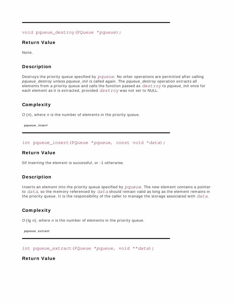
void pqueue_destroy(PQueue *pqueue);
Return Value
None.
Description
Destroys the priority queue specified by pqueue. No other operations are permitted after callingpqueue_destroy unless pqueue_init is called again. The pqueue_destroy operation extracts allelements from a priority queue and calls the function passed as destroy to pqueue_init once foreach element as it is extracted, provided destroy was not set to NULL.
Complexity
O (n), where n is the number of elements in the priority queue.
pqueue_insert
int pqueue_insert(PQueue *pqueue, const void *data);
Return Value
0if inserting the element is successful, or -1 otherwise.
Description
Inserts an element into the priority queue specified by pqueue. The new element contains a pointerto data, so the memory referenced by data should remain valid as long as the element remains inthe priority queue. It is the responsibility of the caller to manage the storage associated with data.
Complexity
O (lg n), where n is the number of elements in the priority queue.
pqueue_extract
int pqueue_extract(PQueue *pqueue, void **data);
Return Value

0if extracting the element is successful, or -1 otherwise.
Description
Extracts the element at the top of the priority queue specified by pqueue. Upon return, data pointsto the data stored in the element that was extracted. It is the responsibility of the caller to managethe storage associated with the data.
Complexity
O (lg n), where n is the number of elements in the priority queue.
pqueue_ peek
void *pqueue_peek(const PQueue *pqueue);
Return Value
Highest priority element in the priority queue, or NULL if the priority queue is empty.
Description
Macro that evaluates to the highest priority element in the priority queue specified by pqueue.
Complexity
O (1)
pqueue_size
int pqueue_size(const PQueue *pqueue);
Return Value
Number of elements in the priority queue.
Description
Macro that evaluates to the number of elements in the priority queue specified by pqueue.

Complexity
O (1)
Top

Mastering Algorithms with CBy Kyle LoudonSlots : 1Table of ContentsChapter 10. Heaps and Priority Queues
Content
10.6 Implementation and Analysis of Priority Queues
There are several ways to implement a priority queue. Perhaps the most intuitive approach is simply tomaintain a sorted set of data. In this approach, the element at the beginning of the sorted set is the onewith the highest priority. However, inserting and extracting elements require resorting the set, which is anO (n ) process in the worst case, where n is the number of elements. Therefore, a better solution is to keepthe set partially ordered using a heap . Recall that the node at the top of a heap is always the one with thehighest priority, however this is defined, and that repairing the heap after inserting and extracting datarequires only O (lg n ) time.
A simple way to implement a priority queue as a heap is to typedef PQueue to Heap (see Example 10.3
). Since the operations of a priority queue are identical to those of a heap, only an interface is designed forpriority queues and the heap datatype serves as the implementation (see Examples Example 10.2 andExample 10.3 ). To do this, each priority queue operation is simply defined to its heap counterpart. The oneexception to this is pqueue_ peek , which has no heap equivalent. This operation works just likepqueue_extract , except that the highest priority element is only returned, not removed.
Example 10.3. Header for the Priority Queue Abstract Datatype
/****************************************************************************** ** ------------------------------- pqueue.h ------------------------------- ** ******************************************************************************/
#ifndef PQUEUE_H#define PQUEUE_H
#include "heap.h"
/*****************************************************************************

* ** Implement priority queues as heaps. ** ******************************************************************************/
typedef Heap PQueue;
/****************************************************************************** ** --------------------------- Public Interface --------------------------- ** ******************************************************************************/
#define pqueue_init heap_init
#define pqueue_destroy heap_destroy
#define pqueue_insert heap_insert
#define pqueue_extract heap_extract
#define pqueue_peek(pqueue) ((pqueue)->tree == NULL ? NULL : (pqueue)->tree[0])
#define pqueue_size heap_size
#endif
Top

Mastering Algorithms with CBy Kyle LoudonSlots : 1Table of ContentsChapter 10. Heaps and Priority Queues
Content
10.7 Priority Queue Example: Parcel Sorting
Most delivery services offer several options for how fast a parcel can be delivered. Generally, the more aperson is willing to pay, the faster the parcel is guaranteed to arrive. Since large delivery services handlemillions of parcels each day, prioritizing parcels during the sorting process is important. This is especiallytrue when space associated with a delivery mechanism becomes limited. In this case, parcels with thehighest priority must go first. For example, if an airplane is making only one more trip for the day back to acentral hub from a busy metropolitan area, all parcels requiring delivery the next day had better be onboard.
One way to ensure that parcels heading to a certain destination are processed according to the correctprioritization is to store information about them in a priority queue. The sorting process begins by scanningparcels into the system. As each parcel is scanned, its information is prioritized in the queue so that whenparcels begin to move through the system, those with the highest priority will go first.
Example 10.4 presents two functions, get_ parcel and put_ parcel , both of which operate on a priority
queue containing parcel records of type Parcel . Parcel is defined in parcel.h , which is not shown. A
sorter calls put_ parcel to load information about a parcel into the system. One member of the Parcelstructure passed to put_ parcel is a priority code. The put_ parcel function inserts a parcel into the priorityqueue, which prioritizes the parcel among the others. When the sorter is ready to move the next parcelthrough the system, it calls get_ parcel . The get_ parcel function fetches the parcel with the next-highestpriority so that parcels are processed in the correct order.
A priority queue is a good way to manage parcels because at any moment, we are interested only in theparcel with the next highest priority. Therefore, we can avoid the overhead of keeping parcels completelysorted. The runtime complexities of get_ parcel and put_ parcel are both O (lg n ) because the twofunctions simply call pqueue_extract and pqueue_insert respectively, which are both O (lg n ) operations.
Example 10.4. Implementation of Functions for Sorting Parcels
/****************************************************************************** *

* ------------------------------- parcels.c ------------------------------ ** ******************************************************************************/
#include <stdlib.h>#include <string.h>
#include "parcel.h"#include "parcels.h"#include "pqueue.h"
/****************************************************************************** ** ------------------------------ get_parcel ------------------------------ ** ******************************************************************************/
int get_parcel(PQueue *parcels, Parcel *parcel) {
Parcel *data;
if (pqueue_size(parcels) == 0)
/************************************************************************** * * * Return that there are no parcels. * * * **************************************************************************/
return -1;
else {
if (pqueue_extract(parcels, (void **)&data) != 0)
/*********************************************************************** * * * Return that a parcel could not be retrieved. * * * ***********************************************************************/
return -1;
else {
/***********************************************************************

* * * Pass back the highest-priority parcel. * * * ***********************************************************************/
memcpy(parcel, data, sizeof(Parcel)); free(data);
}
}
return 0;
}
/****************************************************************************** ** ------------------------------ put_parcel ------------------------------ ** ******************************************************************************/
int put_parcel(PQueue *parcels, const Parcel *parcel) {
Parcel *data;
/****************************************************************************** ** Allocate storage for the parcel. ** ******************************************************************************/
if ((data = (Parcel *)malloc(sizeof(Parcel))) == NULL) return -1;
/****************************************************************************** ** Insert the parcel into the priority queue. ** ******************************************************************************/
memcpy(data, parcel, sizeof(Parcel));
if (pqueue_insert(parcels, data) != 0) return -1;

return 0;
}
Top

Mastering Algorithms with CBy Kyle Loudon
Slots : 1
Table of Contents
Chapter 10. Heaps and Priority Queues
Content
10.8 Questions and Answers
Q: To build a heap from a set of data using the interface presented in this chapter, we callheap_insert once for each element in the set. Since heap_insert runs in O (lg n) time, building a heapof n nodes requires O (n lg n) time. What is an alternative to this approach that runs in O (n) time?
A: An alternative to calling heap_insert repeatedly is to start with an array of nodes that we heapifyby pushing data downward just as is done in heap_insert. In this approach, we first heapify the treewhose root is at position n/2 - 1, then heapify the tree whose root is at position n/2 - 2, andcontinue this process until we heapify the tree rooted at position 0. This approach relies on theobservation that the nodes at n/2 to n - 1 (in a zero-indexed array) are one-node heapsthemselves because they are the leaf nodes. Building a heap in this way is efficient because althoughthere are n/2 - 1 operations that run in O (lg n) time, a tighter analysis reveals that even in theworst case only half the heapifications require comparing data at more than one level. This results inan O (n) running time overall. On the other hand, when calling heap_insert repeatedly, half theheapifications could require traversing all lg n levels in the worst case. Thus, building a heap in thisway runs in O (n lg n) time.
Q: Why are heap_ parent, heap_left, and heap_right defined in heap.c, whereas the other heapmacro, heap_size, is defined in heap.h?
A: The macros heap_ parent, heap_left, and heap_right quickly determine the position of a node'sparent, left child, and right child in a tree represented in an array. The reason these macros are notdefined in heap.h is that they are not a part of the public heap interface. That is, a developer using aheap should not be permitted to traverse a heap's nodes indiscriminately. Instead, access to theheap is restricted to those operations defined by the interface published in heap.h.
Q: Recall that left-balanced binary trees are particularly well-suited to arrays. Why is this not true ofall binary trees?
A: Left-balanced binary trees are particularly well-suited to arrays because no nodes go unusedbetween positions and n - 1, where n is the number of nodes in the tree. Array representations ofbinary trees that are not left-balanced, on the other hand, contain gaps of unused nodes. Forexample, suppose a binary tree of 10 levels is completely full through 9 levels, but in the tenth levelonly 1 node resides at the far right. In contiguous storage, the node at the far right of the tenth levelresides at position 210 - 2 = 1022 (in a zero-indexed array). The node at the far right of the ninthlevel resides at position 29 - 2 = 510. This results in (1022 - 510) - 1= 511 empty positions out ofthe total 1023 positions required to represent the tree. Thus, only 50% of the array is being used.

Q: Suppose we are using a priority queue to prioritize the order in which tasks are scheduled by anapplication. If the system continually processes a large number of high-priority tasks, what problemsmight the system exhibit? How can we correct this?
A: When high-priority elements are continually being inserted into a priority queue, lower-priorityelements may never rise to the top. In a task scheduler, for example, the lower-priority tasks aresaid to be experiencing starvation. To manage this, typically a system employs some mechanism toincrease a task's priority gradually as its time in the queue grows. Thus, even in a busy systemflooded by high-priority tasks, a low-priority task eventually will obtain a high enough priority to riseto the top. Operating systems frequently use an approach like this to ensure that lower-priorityprocesses are not completely starved of CPU time.
Top

Mastering Algorithms with CBy Kyle Loudon
Slots : 1
Table of Contents
Chapter 10. Heaps and Priority Queues
Content
10.9 Related Topics
Fibonacci heaps
Collections of heap-ordered trees. Fibonacci heaps are used sometimes in computing minimumspanning trees and finding single-source shortest paths (see Chapter 17).
k-ary heaps
Heaps built from trees with a branching factor of k. Although not as common as heaps that arebinary trees, a k -ary heap may be worth considering for some problems.
Top

Mastering Algorithms with CBy Kyle Loudon
Slots : 1
Table of Contents
Part II: Data Structures
Content
Chapter 11. GraphsGraphs are some of the most flexible data structures in computing. In fact, most other datastructures can be represented as graphs, although representing them in this way is usually morecomplicated. Generally, graphs are used to model problems defined in terms of relationships orconnections between objects. Objects in a graph may be tangible entities such as nodes in a networkor islands in a river, but they need not be. Often objects are less concrete, such as states in a systemor transactions in a database. The same is true for connections and relationships among the objects.Nodes in a network are physically connected, but the connections between states in a system maysimply indicate a decision made to get from one state to the next. Whatever the case, graphs modelmany useful and interesting computational problems.
This chapter covers:
Graphs
Flexible data structures typically used to model problems defined in terms of relationships orconnections between objects. Objects are represented by vertices, and the relationships orconnections between the objects are represented by edges between the vertices.
Search methods
Techniques for visiting the vertices of a graph in a specific order. Generally, either breadth-firstor depth-first searches are used. Many graph algorithms are based on these basic methods ofsystematically exploring a graph's vertices.
Some applications of graphs are:
Graph algorithms
Algorithms that solve problems modeled by graphs (see Chapter 16). Many graph algorithmssolve problems related to connectivity and routing optimization. For example, Chapter 16explores algorithms for computing minimum spanning trees, finding shortest paths, and solvingthe traveling-salesman problem.
Counting network hops (illustrated in this chapter)
Counting the smallest number of nodes that must be traversed from one node to reach othernodes in an internet. This information is useful in internets in which the most significant costsare directly related to the number of nodes traversed.

Topological sorting (illustrated in this chapter)
A linear ordering of vertices in a directed acyclic graph so that all edges go from left to right.One of the most common uses of topological sorting is in determining an acceptable order inwhich to carry out a number of tasks that depend on one another.
Graph coloring
A process in which we try to color the vertices of a graph so that no two vertices joined by anedge have the same color. Sometimes we are interested only in determining the minimumnumber of colors required to meet this criterion, which is called the graph's chromatic number.
Hamiltonian-cycle problems
Problems in which one works with hamiltonian cycles, paths that pass through every vertex ina graph exactly once before returning to the original vertex. The traveling-salesman problem(see Chapter 16) is a special case of hamiltonian-cycle problem. In the traveling-salesmanproblem, we look for the hamiltonian cycle with the minimum cost.
Clique problems
Problems in which one works with regions of a graph where every vertex is connectedsomehow to every other. Regions with this property are called cliques. Some clique problemsfocus on determining the largest clique that a graph contains. Other clique problems focus ondetermining whether a graph contains a clique of a certain size at all.
Conflict serializability
A significant aspect of database optimization. Rather than executing the instructions oftransactions one transaction after another, database systems typically try to reorder aschedule of instructions to obtain a higher degree of concurrency. However, a serial schedule ofinstructions cannot be reordered arbitrarily; a database system must find a schedule that isconflict serializable. A conflict serializable schedule produces the same results as a serialschedule. To determine if a schedule is conflict serializable, a precedence graph is used todefine relationships among transactions. If the graph does not contain a cycle, the schedule isconflict serializable.
Top

Mastering Algorithms with CBy Kyle Loudon
Slots : 1
Table of Contents
Chapter 11. Graphs
Content
11.1 Description of Graphs
Graphs are composed of two types of elements: vertices and edges. Vertices represent objects, andedges establish relationships or connections between the objects. In many problems, values, orweights, are associated with a graph's edges; however, such problems will not be considered furtheruntil Chapter 16.
Graphs may be either directed or undirected . In a directed graph, edges go from one vertex toanother in a specific direction. Pictorially, a directed graph is drawn with circles for its vertices andarrows for its edges (see Figure 11.1a). Sometimes the edges of a directed graph are referred to asarcs. In an undirected graph, edges have no direction; thus, its edges are depicted using linesinstead of arrows (see Figure 11.1b).
Figure 11.1. Two graphs: (a) a directed graph and (b) an undirectedgraph
Formally, a graph is a pair G = (V, E ), where V is a set of vertices and E is a binary relation on V. Ina directed graph, if an edge goes from vertex u to vertex v, E contains the ordered pair (u, v). Forexample, in Figure 11.1a, V = {1, 2, 3, 4} and E = {(1, 2), (1, 3), (1, 4), (2, 3), (2, 4), (3, 2), (3,4)}. By convention, parentheses are used instead of braces for sets that represent edges in a graph.In an undirected graph, because an edge (u, v) is the same as (v, u), either edge is listed in E, butnot both. Thus, in Figure 11.1b, V = {1, 2, 3, 4} and E = {(1, 2), (1, 3), (1, 4), (2, 3), (2, 4), (3,4)}. Edges may point back to the same vertex in a directed graph, but not in an undirected graph.
Two important relations in graphs are adjacency and incidence. Adjacency is a relation between two
vertices. If a graph contains the edge (u, v), vertex v is said to be adjacent to vertex u. In anundirected graph, this implies that vertex u is also adjacent to vertex v. In other words, theadjacency relation is symmetric in an undirected graph. This is not necessarily true in a directedgraph. For example, in Figure 11.1a, vertex 2 is adjacent to vertex 1, but vertex 1 is not adjacent tovertex 2. On the other hand, vertices 2 and 3 are adjacent to each other. A graph in which everyvertex is adjacent to each other is called complete.
Incidence is a relation between a vertex and an edge. In a directed graph, the edge (u, v) is incidentfrom or leaves vertex u and is incident to or enters vertex v. Thus, in Figure 11.1a, edge (1, 2) isincident from vertex 1 and incident to vertex 2. In a directed graph, the in-degree of a vertex is thenumber of edges incident to it. Its out-degree is the number of edges incident from it. In anundirected graph, the edge (u, v) is incident on vertices u and v. In an undirected graph, the degreeof a vertex is the number of edges incident on it.
Often one talks about paths in a graph. A path is a sequence of vertices traversed by following theedges between them. Formally, a path from one vertex u to another vertex u ' is a sequence ofvertices <v0, v1, v2, . . ., vk > in which u = v0 and u ' = vk , and all (vi - 1, vi ) are in E for i = 1, 2, .. ., k. Such a path contains the edges (v0, v1), (v1, v2), . . ., (vk - 1, vk ) and has a length of k. If apath exists from u to u ', u ' is reachable from u. A path is simple if it has no repeated vertices.
A cycle is a path that includes the same vertex two or more times. That is, in a directed graph, apath is a cycle if one of its edges leaves a vertex and another enters it. Thus, Figure 11.2a containsthe cycle {1, 2, 4, 1}. Formally, in a directed graph, a path forms a cycle if v0 = vk and the pathcontains at least one edge. In an undirected graph, a path <v0, v1, v2, ..., vk > forms a cycle if v0 =vk and no vertices are repeated from v1 to vk . Graphs without cycles are acyclic. Directed acyclicgraphs are given the special name dag (see Figure 11.2b).
Connectivity is another important concept in graphs. An undirected graph is connected if every vertexis reachable from each other by following some path. If this is true in a directed graph, we say thegraph is strongly connected . Although an undirected graph may not be connected, it still maycontain certain sections that are connected, called connected components . If only parts of a directedgraph are strongly connected, the parts are strongly connected components (see Figure 11.3).
Certain vertices have special significance in keeping a graph or connected component connected. Ifremoving a vertex disconnects a graph or component, the vertex is an articulation point . Forexample, in Figure 11.4, vertices 4 and 5 are articulation points because if either of them is removed,the graph becomes disconnected. Upon removing these vertices, the graph has two connectedcomponents, {1, 2, 3} and {6, 7, 8}. Any edge whose removal disconnects a graph is called abridge. A connected graph with no articulation points is biconnected. Although a graph may not bebiconnected, it still may contain biconnected components.
Figure 11.2. Two graphs: (a) a directed graph containing the cycle {1, 2,4, 1}, and (b) a directed acyclic graph, or dag

Figure 11.3. A directed graph with two strongly connected components,{1, 2, 3} and {4, 5, 6}
Figure 11.4. An undirected graph with articulation points 4 and 5, andthe bridge (4, 5)
The most common way to represent a graph in a computer is using an adjacency-list representation.This consists of a linked list of adjacency-list structures. Each structure in the list contains twomembers: a vertex and a list of vertices adjacent to the vertex (see Figure 11.5).
In a graph G = (V, E ), if two vertices u and v in V form an edge (u, v) in E, vertex v is included inthe adjacency list of vertex u. Thus, in a directed graph, the total number of vertices in all adjacencylists is the same as the total number of edges. In an undirected graph, since an edge (u, v) impliesan edge (v, u), vertex v is included in the adjacency list of vertex u, and vertex u is included in the

adjacency list of vertex v. Thus, the total number of vertices in all adjacency lists in this case is twicethe total number of edges.
Figure 11.5. An adjacency-list representation of the directed graph fromFigure 11.3
Typically, adjacency lists are used for graphs that are sparse, that is, graphs in which the number ofedges is less than the number of vertices squared. Sparse graphs are common. However, if a graphis dense , we may choose to represent it using an adjacency-matrix representation (see the relatedtopics at the end of the chapter). Adjacency-matrix representations require O (VE ) space.
11.1.1 Search Methods
Searching a graph means visiting its vertices one at a time in a specific order. There are twoimportant search methods from which many important graph algorithms are derived: breadth-firstsearch and depth-first search.
11.1.1.1 Breadth-first search
Breadth-first search (see Figure 11.6) explores a graph by visiting all vertices adjacent to a vertexbefore exploring the graph further. This search is useful in a number of applications, including findingminimum spanning trees and shortest paths (see Chapter 16 and the first example in this chapter).
Figure 11.6. Breadth-first search starting at vertex 1; vertex 5 isunreachable from 1

To begin, we select a start vertex and color it gray. We color all other vertices in the graph white.The start vertex is also placed alone in a queue. The algorithm then proceeds as follows: for eachvertex in the queue (initially only the start vertex), we peek at the vertex at the front of the queueand explore each vertex adjacent to it. As each adjacent vertex is explored, its color will be white if ithas not been discovered yet. In this case, we color the vertex gray, indicating it has been discovered,and enqueue it at the end of the queue. If its color is not white, it has already been discovered, andthe search proceeds to the next adjacent vertex.
Once all adjacent vertices have been explored, we dequeue the vertex at the front of the queue andcolor it black, indicating we are finished with it. We continue this process until the queue is empty, atwhich point all vertices reachable from the start vertex are black. Figure 11.6 illustrates breadth-firstsearch with a directed graph. Breadth-first search works with undirected graphs as well.
In addition to simply visiting vertices, breadth-first search can be used to keep track of usefulinformation. For example, we can record the number of vertices traversed before reaching eachvertex, which turns out to be the shortest path to each vertex in graphs whose edges are notweighted. In Figure 11.6, the shortest path from vertex 1 to either vertex 2 or 3 consists of one hop,recorded when we first discover vertex 2 and 3. The shortest path from vertex 1 to vertex 4 consistsof two hops: one hop is recorded as we discover vertex 2 from 1, and another is recorded when wediscover vertex 4 from 2. We can also use breadth-first search to generate a breadth-first tree. Abreadth-first tree is the tree formed by maintaining the predecessor of each vertex as we discover it.

Since a vertex is discovered only once (when we color it gray), it has exactly one predecessor, orparent. In Figure 11.6, the edges highlighted in gray are branches of the tree.
11.1.1.2 Depth-first search
Depth-first search (see Figure 11.7) explores a graph by first visiting undiscovered vertices adjacentto the vertex most recently discovered. Thus, the search continually tries to explore as deep as itcan. This makes depth-first search useful in a number of applications, including cycle detection andtopological sorting (see the second example in this chapter).
To begin, we color every vertex white and select a vertex at which to start. The algorithm thenproceeds as follows: first, we color the selected vertex gray to indicate it has been discovered. Then,we select a new vertex from the set of undiscovered vertices adjacent to it, which are white, andrepeat the process. When there are no white vertices adjacent to the currently selected vertex, wehave searched as deep as possible. Thus, we color the currently selected vertex black to indicate thatwe are finished with it, and we backtrack to explore the white vertices adjacent to the previouslyselected vertex.
We continue this process until the vertex we selected as the start vertex has no more white verticesadjacent to it. This process visits only the vertices reachable from the vertex at which we start.Therefore, the entire process must be repeated for each vertex in the graph. For example, in Figure11.7, vertex 4 would not get visited without this step. When we restart at a vertex that is alreadyblack, the search stops immediately, and we move on to the next vertex. Figure 11.7 illustratesdepth-first search with a directed graph. Depth-first search works with undirected graphs as well.
In addition to simply visiting vertices, a depth-first search can be used to keep track of some usefulinformation. For example, we can record the times at which each vertex is discovered and finished.Depth-first search also can be used to produce a depth-first forest. A depth-first forest is a set oftrees, each formed by maintaining the predecessor of each vertex as it is discovered. Since a vertexis discovered only once (when we color it gray), it has exactly one predecessor, or parent. Each treecontains the vertices discovered in searching exactly one connected component. In Figure 11.7, theedges highlighted in gray are branches in the trees.
Figure 11.7. Depth-first search starting at vertex 1

Top

Mastering Algorithms with CBy Kyle LoudonSlots : 1Table of ContentsChapter 11. Graphs
Content
11.2 Interface for Graphsgraph_init
void graph_init(Graph *graph, int (*match)(const void *key1, const void *key2), void (*destroy)(void *data));
Return Value
None.
Description
Initializes the graph specified by graph . This operation must be called for a graph before the graph can
be used with any other operation. The match argument is a function used by various graph operations to
determine if two vertices match. It should return 1 if key1 is equal to key2 , and otherwise. The
destroy argument provides a way to free dynamically allocated data when graph_destroy is called. For
example, if the graph contains data dynamically allocated using malloc , destroy should be set to free to
free the data as the graph is destroyed. For structured data containing several dynamically allocated
members, destroy should be set to a user-defined function that calls free for each dynamically allocated
member as well as for the structure itself. For a graph containing data that should not be freed, destroyshould be set to NULL.
Complexity
O (1)
graph_destroy

void graph_destroy(Graph *graph);
Return Value
None.
Description
Destroys the graph specified by graph . No other operations are permitted after calling graph_destroy
unless graph_init is called again. The graph_destroy operation removes all vertices and edges from a graph
and calls the function passed as destroy to graph_init once for each vertex or edge as it is removed,
provided destroy was not set to NULL.
Complexity
O (V +E ), where V is the number of vertices in the graph and E is the number of edges.
graph_ins_vertex
int graph_ins_vertex(Graph *graph, const void *data);
Return Value
0if inserting the vertex is successful, 1 if the vertex already exists, or -1 otherwise.
Description
Inserts a vertex into the graph specified by graph . The new vertex contains a pointer to data , so the
memory referenced by data should remain valid as long as the vertex remains in the graph. It is the
responsibility of the caller to manage the storage associated with data .
Complexity
O (V ) , where V is the number of vertices in the graph.
graph_ins_edge
int graph_ins_edge(Graph *graph, const void *data1, const void *data2);
Return Value
0if inserting the edge is successful, 1 if the edge already exists, or -1 otherwise.
Description

Inserts an edge from the vertex specified by data1 to the vertex specified by data2 in the graph
specified by graph . Both vertices must have been inserted previously using graph_ins_vertex . The new
edge is represented with a pointer to data2 in the adjacency list of the vertex specified by data1 , so
the memory referenced by data2 should remain valid as long as the edge remains in the graph. It is the
responsibility of the caller to manage the storage associated with data2 . To enter an edge (u , v ) in an
undirected graph, call this operation twice: once to insert an edge from u to v , and again to insert theimplied edge from v to u . This type of representation is common for undirected graphs.
Complexity
O (V ), where V is the number of vertices in the graph.
graph_rem_vertex
int graph_rem_vertex(Graph *graph, void **data);
Return Value
0if removing the vertex is successful, or -1 otherwise.
Description
Removes the vertex matching data from the graph specified by graph . All edges incident to and from
the vertex must have been removed previously using graph_rem_edge . Upon return, data points to the
data stored in the vertex that was removed. It is the responsibility of the caller to manage the storageassociated with the data.
Complexity
O (V + E ), where V is the number of vertices in the graph and E is the number of edges.
graph_rem_edge
int graph_rem_edge(Graph *graph, const void *data1, void **data2);
Return Value
0if removing the edge is successful, or -1 otherwise.
Description
Removes the edge from data1 to data2 in the graph specified by graph . Upon return, data2points to the data stored in the adjacency list of the vertex specified by data1 . It is the responsibility of
the caller to manage the storage associated with the data.

Complexity
O (V ), where V is the number of vertices in the graph.
graph_adjlist
int graph_adjlist(const Graph *graph, const void *data, AdjList **adjlist);
Return Value
0if retrieving the adjacency list is successful, or -1 otherwise.
Description
Retrieves vertices that are adjacent to the vertex specified by data in graph . The adjacent vertices are
returned in the form of an AdjList structure, a structure containing the vertex matching data and a
set of vertices adjacent to it. A pointer to the actual adjacency list in the graph is returned, so it must notbe manipulated by the caller.
Complexity
O (V ), where V is the number of vertices in the graph.
graph_is_adjacent
int graph_is_adjacent(const Graph *graph, const void *data1, const void *data2);
Return Value
1 if the second vertex is adjacent to the first vertex, or otherwise.
Description
Determines whether the vertex specified by data2 is adjacent to the vertex specified by data1 in
graph .
Complexity
O (V ), where V is the number of vertices in the graph.
graph_adjlists
List graph_adjlists(const Graph *graph);

Return Value
List of adjacency-list structures.
Description
Macro that evaluates to the list of adjacency-list structures in graph . Each element in the list is an
AdjList structure. The actual list of adjacency-list structures in the graph is returned, so it must not be
manipulated by the caller.
Complexity
O (1)
graph_vcount
int graph_vcount(const Graph *graph);
Return Value
Number of vertices in the graph.
Description
Macro that evaluates to the number of vertices in the graph specified by graph .
Complexity
O (1)
graph_ecount
int graph_ecount(const Graph *graph);
Return Value
Number of edges in the graph.
Description
Macro that evaluates to the number of edges in the graph specified by graph .
Complexity

O (1)
Top

Mastering Algorithms with CBy Kyle LoudonSlots : 1Table of ContentsChapter 11. Graphs
Content
11.3 Implementation and Analysis of Graphs
An adjacency-list representation of a graph primarily consists of a linked list of adjacency-list structures.Each structure in the list contains two members: a vertex and a list of vertices adjacent to the vertex. In
the implementation presented here, an individual adjacency list is represented by the structure AdjList(see Example 11.1 ). As you would expect, this structure has two members that correspond to those justmentioned. Each adjacency list is implemented as a set (see Chapter 7 ) for reasons discussed in the
questions and answers at the end of the chapter. The structure Graph is the graph data structure (see
Example 11.1 ). This structure consists of five members: vcount is the number of vertices in the graph,
ecount is the number of edges, match and destroy are members used to encapsulate the functions
passed to graph_init , and adjlists is the linked list of adjacency-list structures. Example 11.1 also
defines an enumerated type for vertex colors, which are often used when working with graphs.
Example 11.1. Header for the Graph Abstract Datatype
/****************************************************************************** ** -------------------------------- graph.h ------------------------------- ** ******************************************************************************/
#ifndef GRAPH_H#define GRAPH_H
#include <stdlib.h>
#include "list.h"#include "set.h"
/*****************************************************************************
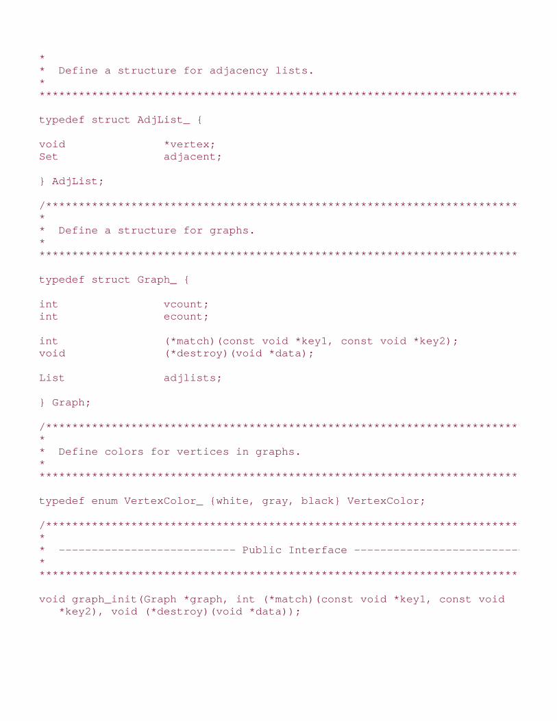
* ** Define a structure for adjacency lists. ** ******************************************************************************/
typedef struct AdjList_ {
void *vertex;Set adjacent;
} AdjList;
/****************************************************************************** ** Define a structure for graphs. ** ******************************************************************************/
typedef struct Graph_ {
int vcount;int ecount;
int (*match)(const void *key1, const void *key2);void (*destroy)(void *data);
List adjlists;
} Graph;
/****************************************************************************** ** Define colors for vertices in graphs. ** ******************************************************************************/
typedef enum VertexColor_ {white, gray, black} VertexColor;
/****************************************************************************** ** --------------------------- Public Interface --------------------------- ** ******************************************************************************/
void graph_init(Graph *graph, int (*match)(const void *key1, const void *key2), void (*destroy)(void *data));

void graph_destroy(Graph *graph);
int graph_ins_vertex(Graph *graph, const void *data);
int graph_ins_edge(Graph *graph, const void *data1, const void *data2);
int graph_rem_vertex(Graph *graph, void **data);
int graph_rem_edge(Graph *graph, void *data1, void **data2);
int graph_adjlist(const Graph *graph, const void *data, AdjList **adjlist);
int graph_is_adjacent(const Graph *graph, const void *data1, const void *data2);
#define graph_adjlists(graph) ((graph)->adjlists)
#define graph_vcount(graph) ((graph)->vcount)
#define graph_ecount(graph) ((graph)->ecount)
#endif
11.3.1 graph_init
The graph_init operation initializes a graph so that it can be used in other operations (see Example 11.2 ).
Initializing a graph is a simple operation in which we set the vcount and ecount members of the graph
to 0, encapsulate the match and destroy functions, and initialize the list of adjacency-list structures.
The runtime complexity of graph_init is O (1) because all of the steps in initializing a graph run in aconstant amount of time.
11.3.2 graph_destroy
The graph_destroy operation destroys a graph (see Example 11.2 ). Primarily this means removing eachadjacency-list structure, destroying the set of vertices it contains, and freeing the memory allocated to its
vertex member by calling the function passed as destroy to graph_init , provided destroy was
not set to NULL.
The runtime complexity of graph_destroy is O (V + E ), where V is the number of vertices in the graph andE is the number of edges. This is because we make V calls to the O (1) operation list_rem_next , and thetotal running time of all calls to set_destroy is O (E ).
11.3.3 graph_ins_vertex
The graph_ins_vertex operation inserts a vertex into a graph (see Example 11.2 ). Specifically, the call

inserts an AdjList structure into the list of adjacency-list structures and sets its vertex member to
point to the data passed by the caller. We begin by ensuring that the vertex does not already exist in the
list. After this, we insert the vertex by calling list_ins_next to insert the AdjList structure at the tail of
the list. Last, we update the count of vertices in the graph by incrementing the vcount member of the
graph data structure.
The runtime complexity of graph_ins_vertex is O (V ), where V is the number of vertices in the graph. Thisis because searching the list of vertices for a duplicate is an O (V ) operation. The call to list_ins_next is O(1).
11.3.4 graph_ins_edge
The graph_ins_edge operation inserts an edge into a graph (see Example 11.2 ). To insert an edge from
the vertex specified by data1 to the vertex specified by data2 , we insert data2 into the adjacency
list of data1 . We begin by ensuring that both vertices exist in the graph. After this, we insert the vertex
specified by data2 into the adjacency list of data1 by calling set_insert . The call to set_insert returns
an error if the edge already exists. Last, we update the count of edges in the graph by incrementing the
ecount member of the graph data structure.
The runtime complexity of graph_ins_edge is O (V ), where V is the number of vertices in the graph. This isbecause searching the list of adjacency-list structures and calling set_insert are both O (V ) operations.
11.3.5 graph_rem_vertex
The graph_rem_vertex operation removes a vertex from a graph (see Example 11.2 ). Specifically, the call
removes an AdjList structure from the list of adjacency-list structures. We begin by ensuring that the
vertex does not exist in any adjacency list, that the vertex does exist in the list of adjacency-list structures,and that the adjacency list of the vertex is empty. After this, we remove the vertex by calling
list_rem_next to remove the appropriate AdjList structure from the list. Last, we update the
count of vertices in the graph by decreasing its vcount member of the graph data structure by 1.
The runtime complexity of graph_rem_vertex is O (V + E ), where V is the number of vertices in the graphand E is the number of edges. This is because searching every adjacency list is O (V + E ), searching the listof adjacency-list structures is O (V ), and calling list_rem_next is O (1).
11.3.6 graph_rem_edge
The graph_rem_edge operation removes an edge from a graph (see Example 11.2 ). Specifically, the call
removes the vertex specified by data2 from the adjacency list of data1 . We begin by ensuring that
the first vertex exists in the graph. Once this has been verified, we remove the edge by calling set_remove
to remove the vertex specified by data2 from the adjacency list of data1 . The call to set_remove
returns an error if data2 is not in the adjacency list of data1 . Last, we update the count of edges in
the graph by decreasing the ecount member of the graph data structure by 1.
The runtime complexity of graph_rem_edge is O (V ), where V is the number of vertices in the graph. Thisis because searching the list of adjacency-list structures and calling set_remove are both O (V ) operations.

11.3.7 graph_adjlist
The graph_adjlist operation returns the AdjList structure containing the set of vertices adjacent to a
specified vertex (see Example 11.2 ). To do this, we search the list of adjacency-list structures until we findthe one that contains the specified vertex.
The runtime complexity of graph_adjlist is O (V ), where V is the number of vertices in the graph. This isbecause searching the list of adjacency-list structures runs in O (V ) time.
11.3.8 graph_is_adjacent
The graph_is_adjacent operation determines whether a specified vertex is adjacent to another (see
Example 11.2 ). To do this, we locate the adjacency-list structure of the vertex specified by data1 and
call set_is_member to determine if data2 is in its adjacency list.
The runtime complexity of graph_adjlist is O (V ), where V is the number of vertices in the graph. This isbecause searching the list of adjacency-list structures and calling set_is_member are both O (V )operations.
11.3.9 graph_adjlists, graph_vcount, graph_ecount
These macros implement some of the simpler graph operations (see Example 11.1 ). Generally, they
provide an interface for accessing and testing members of the Graph structure.
The runtime complexity of these operations is O (1) because accessing members of a structure is a simpletask that runs in a constant amount of time.
Example 11.2. Implementation of the Graph Abstract Datatype
/****************************************************************************** ** -------------------------------- graph.c ------------------------------- ** ******************************************************************************/
#include <stdlib.h>#include <string.h>
#include "graph.h"#include "list.h"#include "set.h"
/****************************************************************************** ** ------------------------------ graph_init ------------------------------ ** *
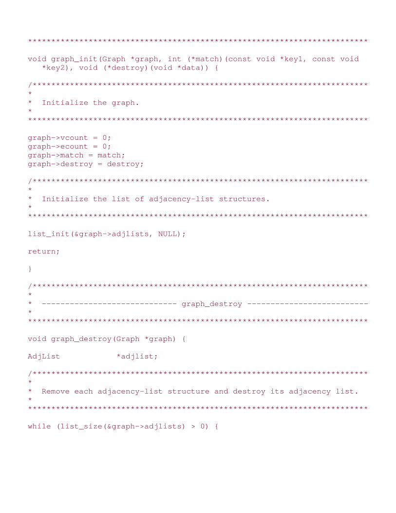
*****************************************************************************/
void graph_init(Graph *graph, int (*match)(const void *key1, const void *key2), void (*destroy)(void *data)) {
/****************************************************************************** ** Initialize the graph. ** ******************************************************************************/
graph->vcount = 0;graph->ecount = 0;graph->match = match;graph->destroy = destroy;
/****************************************************************************** ** Initialize the list of adjacency-list structures. ** ******************************************************************************/
list_init(&graph->adjlists, NULL);
return;
}
/****************************************************************************** ** ----------------------------- graph_destroy ---------------------------- ** ******************************************************************************/
void graph_destroy(Graph *graph) {
AdjList *adjlist;
/****************************************************************************** ** Remove each adjacency-list structure and destroy its adjacency list. ** ******************************************************************************/
while (list_size(&graph->adjlists) > 0) {

if (list_rem_next(&graph->adjlists, NULL, (void **)&adjlist) == 0) {
set_destroy(&adjlist->adjacent);
if (graph->destroy != NULL) graph->destroy(adjlist->vertex);
free(adjlist);
}
}
/****************************************************************************** ** Destroy the list of adjacency-list structures, which is now empty. ** ******************************************************************************/
list_destroy(&graph->adjlists);
/****************************************************************************** ** No operations are allowed now, but clear the structure as a precaution. ** ******************************************************************************/
memset(graph, 0, sizeof(Graph));
return;
}
/****************************************************************************** ** --------------------------- graph_ins_vertex --------------------------- ** ******************************************************************************/
int graph_ins_vertex(Graph *graph, const void *data) {
ListElmt *element;
AdjList *adjlist;
int retval;

/****************************************************************************** ** Do not allow the insertion of duplicate vertices. ** ******************************************************************************/
for (element = list_head(&graph->adjlists); element != NULL; element = list_next(element)) {
if (graph->match(data, ((AdjList *)list_data(element))->vertex)) return 1;
}
/****************************************************************************** ** Insert the vertex. ** ******************************************************************************/
if ((adjlist = (AdjList *)malloc(sizeof(AdjList))) == NULL) return -1;
adjlist->vertex = (void *)data;set_init(&adjlist->adjacent, graph->match, NULL);
if ((retval = list_ins_next(&graph->adjlists, list_tail(&graph->adjlists), adjlist)) != 0) {
return retval;
}
/****************************************************************************** ** Adjust the vertex count to account for the inserted vertex. ** ******************************************************************************/
graph->vcount++;
return 0;
}
/*****************************************************************************

* ** ---------------------------- graph_ins_edge ---------------------------- ** ******************************************************************************/
int graph_ins_edge(Graph *graph, const void *data1, const void *data2) {
ListElmt *element;
int retval;
/****************************************************************************** ** Do not allow insertion of an edge without both its vertices in the graph. ** ******************************************************************************/
for (element = list_head(&graph->adjlists); element != NULL; element = list_next(element)) {
if (graph->match(data2, ((AdjList *)list_data(element))->vertex)) break;
}
if (element == NULL) return -1;
for (element = list_head(&graph->adjlists); element != NULL; element = list_next(element)) {
if (graph->match(data1, ((AdjList *)list_data(element))->vertex)) break;
}
if (element == NULL) return -1;
/****************************************************************************** ** Insert the second vertex into the adjacency list of the first vertex. ** ******************************************************************************/
if ((retval = set_insert(&((AdjList *)list_data(element))->adjacent, data2))

!= 0) {
return retval;
}
/****************************************************************************** ** Adjust the edge count to account for the inserted edge. ** ******************************************************************************/
graph->ecount++;
return 0;
}
/****************************************************************************** ** --------------------------- graph_rem_vertex --------------------------- ** ******************************************************************************/
int graph_rem_vertex(Graph *graph, void **data) {
ListElmt *element, *temp, *prev;
AdjList *adjlist;
int found;
/****************************************************************************** ** Traverse each adjacency list and the vertices it contains. ** ******************************************************************************/
prev = NULL;found = 0;
for (element = list_head(&graph->adjlists); element != NULL; element = list_next(element)) {

/************************************************************************** * * * Do not allow removal of the vertex if it is in an adjacency list. * * * **************************************************************************/
if (set_is_member(&((AdjList *)list_data(element))->adjacent, *data)) return -1;
/************************************************************************** * * * Keep a pointer to the vertex to be removed. * * * **************************************************************************/
if (graph->match(*data, ((AdjList *)list_data(element))->vertex)) { temp = element; found = 1;
}
/************************************************************************** * * * Keep a pointer to the vertex before the vertex to be removed. * * * **************************************************************************/
if (!found) prev = element;
} /****************************************************************************** ** Return if the vertex was not found. ** ******************************************************************************/
if (!found) return -1;
/****************************************************************************** ** Do not allow removal of the vertex if its adjacency list is not empty. ** *
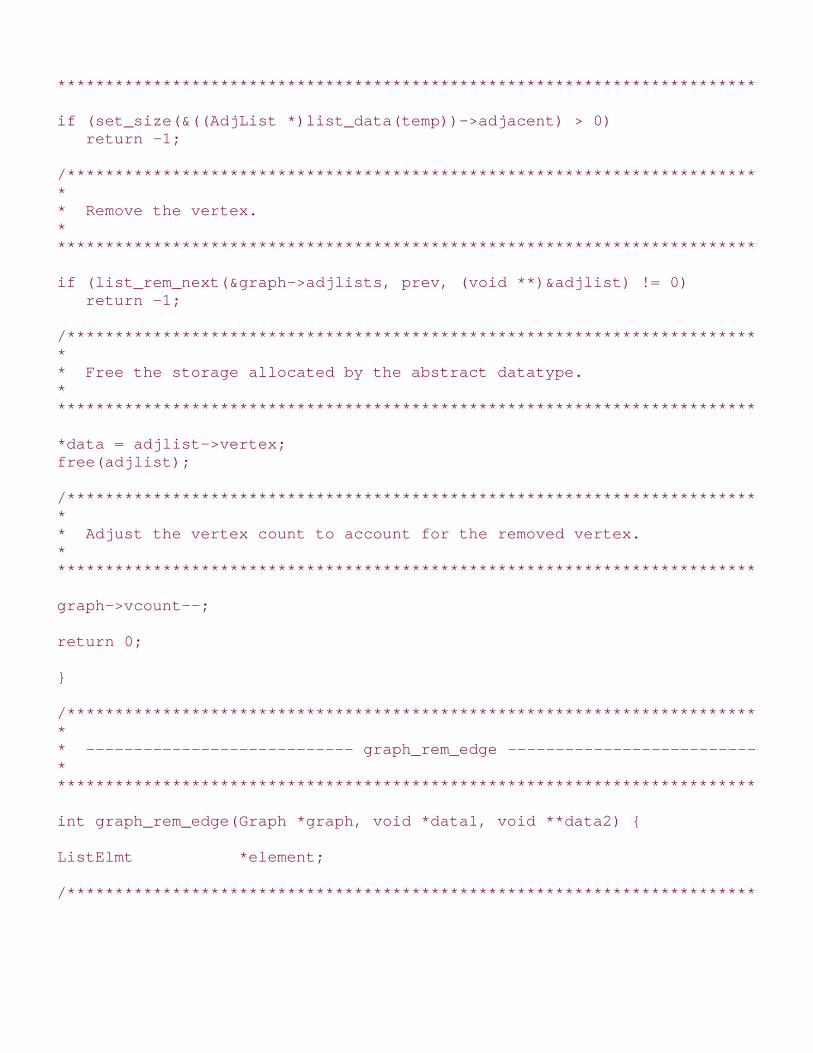
*****************************************************************************/
if (set_size(&((AdjList *)list_data(temp))->adjacent) > 0) return -1;
/****************************************************************************** ** Remove the vertex. ** ******************************************************************************/
if (list_rem_next(&graph->adjlists, prev, (void **)&adjlist) != 0) return -1;
/****************************************************************************** ** Free the storage allocated by the abstract datatype. ** ******************************************************************************/
*data = adjlist->vertex;free(adjlist);
/****************************************************************************** ** Adjust the vertex count to account for the removed vertex. ** ******************************************************************************/
graph->vcount--;
return 0;
}
/****************************************************************************** ** ---------------------------- graph_rem_edge ---------------------------- ** ******************************************************************************/
int graph_rem_edge(Graph *graph, void *data1, void **data2) {
ListElmt *element;
/*****************************************************************************

* ** Locate the adjacency list for the first vertex. ** ******************************************************************************/
for (element = list_head(&graph->adjlists); element != NULL; element = list_next(element)) {
if (graph->match(data1, ((AdjList *)list_data(element))->vertex)) break;
}
if (element == NULL) return -1;
/****************************************************************************** ** Remove the second vertex from the adjacency list of the first vertex. ** ******************************************************************************/
if (set_remove(&((AdjList *)list_data(element))->adjacent, data2) != 0) return -1;
/****************************************************************************** ** Adjust the edge count to account for the removed edge. ** ******************************************************************************/
graph->ecount--;
return 0;
}
/****************************************************************************** ** ----------------------------- graph_adjlist ---------------------------- ** ******************************************************************************/
int graph_adjlist(const Graph *graph, const void *data, AdjList **adjlist) {
ListElmt *element,

*prev;
/****************************************************************************** ** Locate the adjacency list for the vertex. ** ******************************************************************************/
prev = NULL;
for (element = list_head(&graph->adjlists); element != NULL; element = list_next(element)) {
if (graph->match(data, ((AdjList *)list_data(element))->vertex)) break;
prev = element;
}
/****************************************************************************** ** Return if the vertex was not found. ** ******************************************************************************/
if (element == NULL) return -1;
/****************************************************************************** ** Pass back the adjacency list for the vertex. ** ******************************************************************************/
*adjlist = list_data(element);
return 0;
}
/****************************************************************************** ** --------------------------- graph_is_adjacent -------------------------- ** ******************************************************************************/

int graph_is_adjacent(const Graph *graph, const void *data1, const void *data2) {
ListElmt *element, *prev;
/****************************************************************************** ** Locate the adjacency list of the first vertex. ** ******************************************************************************/
prev = NULL;
for (element = list_head(&graph->adjlists); element != NULL; element = list_next(element)) {
if (graph->match(data1, ((AdjList *)list_data(element))->vertex)) break;
prev = element;
}
/****************************************************************************** ** Return if the first vertex was not found. ** ******************************************************************************/
if (element == NULL) return 0;
/****************************************************************************** ** Return whether the second vertex is in the adjacency list of the first. ** ******************************************************************************/
return set_is_member(&((AdjList *)list_data(element))->adjacent, data2);
}

Top

Mastering Algorithms with CBy Kyle LoudonSlots : 1Table of ContentsChapter 11. Graphs
Content
11.4 Graph Example: Counting Network Hops
Graphs play an important part in solving many networking problems . One problem, for example, isdetermining the best way to get from one node to another in an internet , a network of gateways into othernetworks. One way to model an internet is using an undirected graph in which vertices represent nodes,and edges represent connections between the nodes. With this model, we can use breadth-first search tohelp determine the smallest number of traversals, or hops , between various nodes.
For example, consider the graph in Figure 11.8 , which represents an internet of six nodes. Starting atnode1, there is more than one way we can reach node4. The paths <node1, node2, node4>, <node1,node3, node2, node4>, and <node1, node3, node5, node4> are all acceptable. Breadth-first searchdetermines the shortest path, <node1, node2, node4>, which requires two hops.
Figure 11.8. Hop counts after performing a breadth-first search on aninternet of six nodes
This example presents a function, bfs (see Examples Example 11.3 and Example 11.4 ), that implementsbreadth-first search. It is used here to determine the smallest number of hops between nodes in an

internet. The function has three arguments: graph is a graph, which in this problem represents the
internet; start is the vertex representing the starting point; and hops is the list of hop counts that is
returned. The function modifies graph , so a copy should be made before calling the function, if
necessary. Also, vertices returned in hops are pointers to the actual vertices from graph , so the caller
must ensure that the storage in graph remains valid as long as hops is being accessed. Each vertex in
graph is a BfsVertex structure (see Example 11.3 ), which has three members: data is a pointer to
the data associated with the vertex, color maintains the color of the vertex during the search, and
hops maintains the number of hops to the vertex from the start node. The match function for graph ,
which is set by the caller when initializing the graph with graph_init , should compare only the datamembers of BfsVertex structures.
The bfs function performs breadth-first search as described earlier in this chapter. To keep track of theminimum number of hops to each vertex, we set the hop count of each vertex to the hop count of thevertex to which it is adjacent plus 1. We do this for each vertex as we discover it, and color it gray. Colors
and hop counts for each vertex are maintained by the BfsVertex structures in the list of adjacency-list
structures. At the end, we load hops with all vertices whose hop counts are not -1. These are the vertices
that were reachable from the start node.
The runtime complexity of bfs is O (V + E ), where V is the number of vertices in the graph and E is thenumber of edges. This is because initializing the colors of the vertices and ensuring that the start nodeexists both run in O (V ) time, the loop in which the breadth-first search is performed in O (V + E ) time,and loading the list of hop counts is O (V ).
Example 11.3. Header for Breadth-First Search
/****************************************************************************** ** --------------------------------- bfs.h -------------------------------- ** ******************************************************************************/
#ifndef BFS_H#define BFS_H
#include "graph.h"#include "list.h"
/****************************************************************************** ** Define a structure for vertices in a breadth-first search. ** ******************************************************************************/
typedef struct BfsVertex_ {
void *data;

VertexColor color;int hops;
} BfsVertex;
/****************************************************************************** ** --------------------------- Public Interface --------------------------- ** ******************************************************************************/
int bfs(Graph *graph, BfsVertex *start, List *hops);
#endif
Example 11.4. Implementation of a Function for Breadth-First Search
/****************************************************************************** ** -------------------------------- bfs.c --------------------------------- ** ******************************************************************************/
#include <stdlib.h>
#include "bfs.h"#include "graph.h"#include "list.h"#include "queue.h"
/****************************************************************************** ** --------------------------------- bfs ---------------------------------- ** ******************************************************************************/
int bfs(Graph *graph, BfsVertex *start, List *hops) {
Queue queue;
AdjList *adjlist, *clr_adjlist;
BfsVertex *clr_vertex, *adj_vertex;

ListElmt *element, *member;
/****************************************************************************** ** Initialize all of the vertices in the graph. ** ******************************************************************************/
for (element = list_head(&graph_adjlists(graph)); element != NULL; element = list_next(element)) {
clr_vertex = ((AdjList *)list_data(element))->vertex;
if (graph->match(clr_vertex, start)) {
/*********************************************************************** * * * Initialize the start vertex. * * * ***********************************************************************/
clr_vertex->color = gray; clr_vertex->hops = 0;
}
else {
/*********************************************************************** * * * Initialize vertices other than the start vertex. * * * ***********************************************************************/
clr_vertex->color = white; clr_vertex->hops = -1;
}
}
/****************************************************************************** ** Initialize the queue with the adjacency list of the start vertex. ** *

*****************************************************************************/
queue_init(&queue, NULL);
if (graph_adjlist(graph, start, &clr_adjlist) != 0) {
queue_destroy(&queue); return -1;
}
if (queue_enqueue(&queue, clr_adjlist) != 0) {
queue_destroy(&queue); return -1;
}
/****************************************************************************** ** Perform breadth-first search. ** ******************************************************************************/
while (queue_size(&queue) > 0) {
adjlist = queue_peek(&queue);
/************************************************************************** * * * Traverse each vertex in the current adjacency list. * * * **************************************************************************/
for (member = list_head(&adjlist->adjacent); member != NULL; member = list_next(member)) {
adj_vertex = list_data(member);
/*********************************************************************** * * * Determine the color of the next adjacent vertex. * * * ***********************************************************************/
if (graph_adjlist(graph, adj_vertex, &clr_adjlist) != 0) {

queue_destroy(&queue); return -1;
}
clr_vertex = clr_adjlist->vertex;
/*********************************************************************** * * * Color each white vertex gray and enqueue its adjacency list. * * * ***********************************************************************/
if (clr_vertex->color == white) {
clr_vertex->color = gray; clr_vertex->hops = ((BfsVertex *)adjlist->vertex)->hops + 1;
if (queue_enqueue(&queue, clr_adjlist) != 0) {
queue_destroy(&queue); return -1;
}
}
}
/************************************************************************** * * * Dequeue the current adjacency list and color its vertex black. * * * **************************************************************************/
if (queue_dequeue(&queue, (void **)&adjlist) == 0) {
((BfsVertex *)adjlist->vertex)->color = black;
}
else {
queue_destroy(&queue); return -1;

}
}
queue_destroy(&queue);
/****************************************************************************** ** Pass back the hop count for each vertex in a list. ** ******************************************************************************/
list_init(hops, NULL);
for (element = list_head(&graph_adjlists(graph)); element != NULL; element = list_next(element)) {
/************************************************************************** * * * Skip vertices that were not visited (those with hop counts of -1). * * * **************************************************************************/
clr_vertex = ((AdjList *)list_data(element))->vertex;
if (clr_vertex->hops != -1) {
if (list_ins_next(hops, list_tail(hops), clr_vertex) != 0) {
list_destroy(hops); return -1;
}
}
}
return, 0;
}

Top

Mastering Algorithms with CBy Kyle LoudonSlots : 1Table of ContentsChapter 11. Graphs
Content
11.5 Graph Example: Topological Sorting
Sometimes we encounter problems in which we must determine an acceptable ordering by which to carryout tasks that depend on one another. Imagine a set of classes at a university that have prerequisites, or acomplicated project in which certain phases must be completed before other phases can begin. To modelproblems like these, we use a directed graph, called a precedence graph , in which vertices represent tasksand edges represent dependencies between them. To show a dependency, we draw an edge from the taskthat must be completed first to the task that depends on it.
For example, consider the directed acyclic graph in Figure 11.9 a, which represents a curriculum of sevencourses and their prerequisites: CS100 has no prerequisites, CS200 requires CS100, CS300 requires CS200and MA100, MA100 has no prerequisites, MA200 requires MA100, MA300 requires CS300 and MA200, andCS150 has no prerequisites and is not a prerequisite itself.
Figure 11.9. Courses and their prerequisites (a) in a directed acrylic graphand (b) in one topological sorting
Depth-first search helps to determine an acceptable ordering by performing a topological sort on the

courses. Topological sorting orders the vertices in a directed acyclic graph so that all edges go from left toright. In the problem involving course prerequisites, this means that all prerequisites will appear to the leftof the courses that require them (see Figure 11.9 b). Formally, a topological sort of a directed acyclic graphG = (V , E ) is a linear ordering of its vertices so that if an edge (u , v ) exists in G , then u appears beforev in the linear ordering. In many cases, there is more than one ordering that satisfies this.
This example presents a function, dfs (see Examples Example 11.5 and Example 11.6 ), that implementsdepth-first search. It is used here to sort a number of tasks topologically. The function has two arguments:
graph is a graph, which in this problem represents the tasks to be ordered, and ordered is the list of
topologically sorted vertices that is returned. The function modifies graph , so a copy should be made
before calling the function, if necessary. Also, vertices returned in ordered are pointers to the actual
vertices from graph , so the caller must ensure that the storage in graph remains valid as long as
ordered is being accessed. Each vertex in graph is a DfsVertex structure (see Example 11.5 ),
which has two members: data is a pointer to the data associated with the vertex, and color maintains
the color of the vertex during the search. The match function for graph , which is set by the caller
when initializing the graph with graph_init , should compare only the data members of DfsVertexstructures.
The dfs function performs depth-first search as described earlier in this chapter. The function dfs_main isthe actual function that executes the search. The last loop in dfs ensures that we end up searching allcomponents of graphs that are not connected, such as the one in Figure 11.9 a. As each vertex is finished
and colored black in dfs_main , it is inserted at the head of ordered . At the end, ordered contains
the topologically sorted list of vertices.
The runtime complexity of dfs is O (V + E ), where V is the number of vertices in the graph and E is thenumber of edges. This is because initializing the colors of the vertices runs in O (V ) time, and the calls todfs_main run in O (V + E ) overall.
Example 11.5. Header for Depth-First Search
/****************************************************************************** ** -------------------------------- dfs.h --------------------------------- ** ******************************************************************************/
#ifndef DFS_H#define DFS_H
#include "graph.h"#include "list.h"
/****************************************************************************** ** Define a structure for vertices in a depth-first search. ** ******************************************************************************/

typedef struct DfsVertex_ {
void *data;
VertexColor color;
} DfsVertex;
/****************************************************************************** ** --------------------------- Public Interface --------------------------- ** ******************************************************************************/
int dfs(Graph *graph, List *ordered);
#endif
Example 11.6. Implementation of a Function for Depth-First Search
/****************************************************************************** ** -------------------------------- dfs.c --------------------------------- ** ******************************************************************************/
#include <stdlib.h>
#include "dfs.h"#include "graph.h"#include "list.h"
/****************************************************************************** ** ------------------------------- dfs_main ------------------------------- ** ******************************************************************************/
static int dfs_main(Graph *graph, AdjList *adjlist, List *ordered) {
AdjList *clr_adjlist;
DfsVertex *clr_vertex, *adj_vertex;
ListElmt *member;

/****************************************************************************** ** Color the vertex gray and traverse its adjacency list. ** ******************************************************************************/
((DfsVertex *)adjlist->vertex)->color = gray;
for (member = list_head(&adjlist->adjacent); member != NULL; member = list_next(member)) {
/************************************************************************** * * * Determine the color of the next adjacent vertex. * * * **************************************************************************/
adj_vertex = list_data(member);
if (graph_adjlist(graph, adj_vertex, &clr_adjlist) != 0) return -1;
clr_vertex = clr_adjlist->vertex;
/************************************************************************** * * * Move one vertex deeper when the next adjacent vertex is white. * * * **************************************************************************/
if (clr_vertex->color == white) {
if (dfs_main(graph, clr_adjlist, ordered) != 0) return -1;
}
}
/****************************************************************************** ** Color the current vertex black and make it first in the list. ** ******************************************************************************/

((DfsVertex *)adjlist->vertex)->color = black;
if (list_ins_next(ordered, NULL, (DfsVertex *)adjlist->vertex) != 0) return -1;
return 0;
}
/****************************************************************************** ** ---------------------------------- dfs --------------------------------- ** ******************************************************************************/
int dfs(Graph *graph, List *ordered) {
DfsVertex *vertex;
ListElmt *element;
/****************************************************************************** ** Initialize all of the vertices in the graph. ** ******************************************************************************/
for (element = list_head(&graph_adjlists(graph)); element != NULL; element = list_next(element)) {
vertex = ((AdjList *)list_data(element))->vertex; vertex->color = white;
}
/****************************************************************************** ** Perform depth-first search. ** ******************************************************************************/
list_init(ordered, NULL);
for (element = list_head(&graph_adjlists(graph)); element != NULL; element = list_next(element)) {

/************************************************************************** * * * Ensure that every component of unconnected graphs is searched. * * * **************************************************************************/
vertex = ((AdjList *)list_data(element))->vertex;
if (vertex->color == white) {
if (dfs_main(graph, (AdjList *)list_data(element), ordered) != 0) {
list_destroy(ordered); return -1;
}
}
}
return 0;
}
Top

Mastering Algorithms with CBy Kyle Loudon
Slots : 1
Table of Contents
Chapter 11. Graphs
Content
11.6 Questions and Answers
Q: In the graph implementation presented in this chapter, why is a linked list used for the list ofadjacency-list structures but sets are used for the adjacency lists?
A: Many adjacency-list representations of graphs consist of an array of adjacency lists, with eachelement in the array corresponding to one vertex in the graph. The implementation in this chapterdeviates from this model. First, it uses a linked list in place of the array because the list candynamically expand and contract as we insert and remove vertices. Second, it uses sets for theadjacency lists because the vertices they contain are not ordered, and the primary operationsassociated with adjacency lists (inserting and removing vertices, and testing for membership) arewell-suited to the set abstract datatype presented earlier. Perhaps the list of adjacency-list structurescould have been implemented using a set as well, but this was ruled out because the primaryoperation here is to locate the adjacency lists of specific vertices. A linked list is better suited to thisthan a set.
Q: Suppose we model an internet using a graph (as shown earlier in this chapter) and we determinethat the graph contains an articulation point. What are the implications of this?
A: Graphs have many important uses in network problems. If in a graph modeling an internet wedetermine that there is an articulation point, the articulation point represents a single point of failure.Thus, if a system residing at an articulation point goes down, other systems are forced into differentconnected components and as a result will no longer be able to communicate with each other.Therefore, in designing large networks in which connectivity is required at all times, it is importantthat there be no articulation points. We can curb this problem by placing redundancies in thenetwork.
Q: Consider a graph that models a structure of airways, highways in the sky on which airplanes areoften required to fly. The structure consists of two types of elements: navigational facilities, callednavaids for short, and airways that connect navaids, which are typically within a hundred miles ofeach other. Airways may be bidirectional or one-way. At certain times some airways are not availablefor use. Suppose during one of these times we would like to determine whether we can still reach aparticular destination. How can we determine this? What is the runtime complexity of solving thisproblem?
A: If we perform breadth-first search from our starting point in the airway structure, we can reachany destination if we discover it during the search. Otherwise, the destination must reside in acomponent of the graph that became unreachable when an airway was made unavailable. The closed

airway constitutes a bridge in the graph. This problem can be solved in O (V + E ) time, where V isthe number of navaids and E is the number of airways in the structure. This is the runtimecomplexity of breadth-first search.
Q: Suppose we would like to use a computer to model states in a system. For example, imagine thevarious states of a traffic-light system at an intersection and the decisions the system has to make.How can we use a graph to model this?
A: Directed graphs are good for modeling state machines, such as the traffic-light system mentionedhere. In a directed graph, we let vertices represent the various states, and edges represent thedecisions made to get from one state to another. Edges in the graph are directed because a decisionmade to get from one state to the next does not imply that the decision can be reversed.
Q: When discussing depth-first search, it was mentioned that sometimes it is useful to keep track ofdiscovery and finishing times for each vertex. The start time of a vertex is a sequence numberrecorded when the vertex is discovered for the first time and we color it gray. The finishing time of avertex is a sequence number recorded when we are finished with the vertex and color it black. In theimplementation of depth-first search presented in this chapter, these times were not recorded. Howcould we modify the implementation to record them?
A: Discovery and finishing times recorded during depth-first search are important to somealgorithms. To record these times, we use a counter that increments itself each time we color avertex either gray or black. As a vertex is colored gray, we record the current value of the counter asits discovery time. As a vertex is colored black, we record the current value of the counter as itsfinishing time. In the implementation presented in this chapter, we could add two members to theDfsVertex structure to keep track of these times for each vertex.
Q: The transpose of a directed graph is a graph with the direction of its edges reversed. Formally, fora directed graph G = (V, E ), its transpose is indicated as G T. How could we form the transpose of agraph assuming an adjacency-list representation? What is the runtime complexity of this?
A: To form the transpose G T of a graph G = (V, E ), we traverse the adjacency list of each vertex uin V. As we traverse each list, we make sure that vertex v and u have both been inserted into G T bycalling graph_ins_vertex for each vertex. Next, we call graph_ins_edge to insert an edge from v to uinto G T. Each call to graph_ins_vertex runs in O (V ) time. This operation is called 2E times, where Eis the number of edges in G. Of course, some of these calls will not actually insert the vertex if it wasinserted previously. Each call to graph_ins_edge runs in O (V ) time. This operation is called once foreach edge in G as well. Thus, using this approach, the overall time to transpose a graph is O (V E ).
Q: At the start of this chapter, it was mentioned that many data structures can be represented asgraphs. How might we think of a binary tree as a graph?
A: A binary tree is a directed acyclic graph with the following characteristics. Each node has up to twoedges incident from it and one edge incident to it, except for the root node, which has only the twoedges incident from it. Edges incident from a vertex connect it with its children. The edge incident toa vertex connects its parent to it. Thus, the adjacency list of each vertex contains its children.
Top

Mastering Algorithms with CBy Kyle Loudon
Slots : 1
Table of Contents
Chapter 11. Graphs
Content
11.7 Related Topics
Hypergraphs
Graphs similar to undirected graphs but which contain hyperedges. Hyperedges are edges thatconnect an arbitrary number of vertices. In general, most operations and algorithms forgraphs, such as the ones described in this chapter, can be adapted to work with hypergraphsas well.
Multigraphs
Graphs similar to undirected graphs but which allow multiple edges between the same twovertices. As with hypergraphs, in general, most operations and algorithms for graphs can beadapted to work with multigraphs as well.
Adjacency-matrix representation
A graph representation that consists of a V x V matrix, where V is the number of vertices in thegraph. If an edge exists between two vertices u and v, we set a flag in position [u, v ] in thematrix. An adjacency-matrix representation is typically used for dense graphs, in which thenumber of edges is close to the number of vertices squared. Although the interface presentedin this chapter may appear to reflect the specifics of an adjacency-list representation, there arethings we could do to support this interface for an adjacency-matrix representation as well,thus keeping the details of the actual implementation hidden.
Top

Mastering Algorithms with CBy Kyle Loudon
Slots : 1
Table of Contents
Content
Part III: AlgorithmsThis part of the book contains six chapters on algorithms. Chapter 12, covers various algorithmsfor sorting, including insertion sort, quicksort, merge sort, counting sort, and radix sort.Chapter 12 also presents binary search. Chapter 13, covers numerical methods, includingalgorithms for polynomial interpolation, least-squares estimation, and the solution of equationsusing Newton's method. Chapter 14, presents algorithms for data compression, includingHuffman coding and LZ77. Chapter 15, presents algorithms for DES and RSA encryption.Chapter 16, covers graph algorithms, including Prim's algorithm for minimum spanning trees,Dijkstra's algorithm for shortest paths, and an algorithm for solving the traveling-salesmanproblem. Chapter 17, presents geometric algorithms, including methods for testing whether linesegments intersect, computing convex hulls, and computing arc lengths on spherical surfaces.
Top

Mastering Algorithms with CBy Kyle Loudon
Slots : 1
Table of Contents
Part III: Algorithms
Content
Chapter 12. Sorting and SearchingSorting means arranging a set of elements in a prescribed order. Normally a sort is thought of aseither ascending or descending. An ascending sort of the integers {5, 2, 7, 1}, for example, produces{1, 2, 5, 7}, whereas a descending sort produces {7, 5, 2, 1}. In general, sorting serves to organizedata so that it is more meaningful. Although the most visible application of sorting is sorting data todisplay it, often sorting is used to organize data in solving other problems, sometimes as a part ofother formal algorithms.
In general, sorting algorithms are divided into two classes: comparison sorts and linear-time sorts.Comparison sorts rely on comparing elements to place them in the correct order. Surprisingly, not allsorting algorithms rely on making comparisons. For those that do, it is not possible to sort fasterthan in O (n lg n) time. Linear-time sorts get their name from sorting in a time proportional to thenumber of elements being sorted, or O (n). Unfortunately, linear-time sorts rely on certaincharacteristics in the data, so we cannot always apply them. Some sorts use the same storage thatcontains the data to store output as the sort proceeds; these are called in-place sorts. Others requireextra storage for the output data, although they may copy the results back over the original data atthe end.
Searching is the ubiquitous task of locating an element in a set of data. The simplest approach tolocating an element takes very little thought: we simply scan the set from one end to the other. Thisis called linear search . Generally, it is used with data structures that do not support random accessvery well, such as linked lists (see Chapter 5). An alternative approach is to use binary search, whichis presented in this chapter. Other approaches rely on data structures developed specifically forsearching, such as hash tables (see Chapter 8) and binary search trees (see Chapter 9). This chaptercovers:
Insertion sort
Although not the most efficient sorting algorithm, insertion sort has the virtue of simplicity andthe ability to sort in place. Its best application is for incremental sorting on small sets of data.
Quicksort
An in-place sorting algorithm widely regarded as the best for sorting in the general case. Itsbest application is for medium to large sets of data.
Merge sort
An algorithm with essentially the same performance as quicksort, but with twice its storage

requirements. Ironically, its best application is for very large sets of data because it inherentlyfacilitates working with divisions of the original unsorted set.
Counting sort
A stable, linear-time sorting algorithm that works with integers for which we know the largestvalue. Its primary use is in implementing radix sort.
Radix sort
A linear-time sorting algorithm that sorts elements digit by digit. Radix sort is well suited toelements of a fixed size that can be conveniently broken into pieces, expressible as integers.
Binary search
An effective way to search sorted data in which we do not expect frequent insertions ordeletions. Since resorting a set of data is expensive relative to searching it, binary search isbest when the data does not change.
Some applications of sorting and searching algorithms are:
Order statistics
Finding the i th smallest element in a set. One simplistic approach is to select the i th elementout of the set once it has been sorted.
Binary search
An efficient search method that relies on sorted data. Binary search works fundamentally bydividing a sorted set of data repeatedly and inspecting the element in the middle of eachdivision.
Directory listings (illustrated in this chapter)
Listings of files in a file system that have been organized into groups. Generally, an operatingsystem will sort a directory listing in some manner before displaying it.
Database systems
Typically, large systems containing vast amounts of data that must be stored and retrievedquickly. The amount of data generally stored in databases makes an efficient and flexibleapproach to searching the data essential.
Spell checkers (illustrated in this chapter)
Programs that check the spelling of words in text. Validation is performed against words in adictionary. Since spell checkers frequently deal with long strings of text containing manythousands of words, they must be able to search the set of acceptable words efficiently.
Spreadsheets
An important part of most businesses for managing inventory and financial data. Spreadsheetstypically contain diverse data that is more meaningful when sorted.
Top

Mastering Algorithms with CBy Kyle Loudon
Slots : 1
Table of Contents
Chapter 12. Sorting and Searching
Content
12.1 Description of Insertion Sort
Insertion sort is one of the simplest sorting algorithms. It works like the approach we might use tosystematically sort a pile of canceled checks by hand. We begin with a pile of unsorted checks andspace for a sorted pile, which initially contains no checks. One at a time, we remove a check from theunsorted pile and, considering its number, insert it at the proper position among the sorted checks.More formally, insertion sort takes one element at a time from an unsorted set and inserts it into asorted one by scanning the set of sorted elements to determine where the new element belongs.Although at first it may seem that insertion sort would require space for both the sorted and unsortedsets of data independently, it actually sorts in place.
Insertion sort is a simple algorithm, but it is inefficient for large sets of data. This is becausedetermining where each element belongs in the sorted set potentially requires comparing it withevery other element in the sorted set thus far. An important virtue of insertion sort, however, is thatinserting a single element into a set that is already sorted requires only one scan of the sortedelements, as opposed to a complete run of the algorithm. This makes insertion sort efficient forincremental sorting. This situation might occur, for example, in a reservation system of a large hotel.Suppose one display in the system lists all guests, sorted by name, and is updated in real time asnew guests check in. Using insertion sort, resorting requires only a single sweep of the data to inserta new name into the list.
Top

Mastering Algorithms with CBy Kyle LoudonSlots : 1Table of ContentsChapter 12. Sorting and Searching
Content
12.2 Interface for Insertion Sortissort
int issort(void *data, int size, int esize, int (*compare)(const void *key1, const void *key2));
Return Value
0 if sorting is successful, or -1 otherwise.
Description
Uses insertion sort to sort the array of elements in data . The number of elements in data is specified
by size . The size of each element is specified by esize . The function pointer compare specifies a
user-defined function to compare elements. This function should return 1 if key1 > key2 , if key1 =
key2 , and -1 if key1 < key2 for an ascending sort. For a descending sort, compare should reverse
the cases returning 1 and -1. When issort returns, data contains the sorted elements.
Complexity
O (n 2 ), where n is the number of elements to be sorted.
Top

Mastering Algorithms with CBy Kyle LoudonSlots : 1Table of ContentsChapter 12. Sorting and Searching
Content
12.3 Implementation and Analysis of Insertion Sort
Insertion sort works fundamentally by inserting elements from an unsorted set one at a time into a sorted
set. In the implementation presented here, both of these sets reside in data , a single block of contiguous
storage. Initially, data contains the unsorted set consisting of size elements. As issort runs, datagradually becomes consumed by the sorted set until when issort returns, data is completely sorted.
Although this implementation uses contiguous storage, insertion sort can easily be adapted to work withlinked lists efficiently, something not all sorts can claim.
Insertion sort revolves around a single nested loop (see Example 12.1 ). The outer loop, j , controls which
element from the unsorted set is currently being inserted among the sorted elements. Since the element
just to the right of the sorted set is always the next to be inserted, we can also think of j as the position
dividing the sorted and unsorted sets in data . For each element at position j , an inner loop, i , is
used to cycle backward through the set of sorted elements until the proper position for the element is
found. As we move backward through the set, each element at position i is copied one position to the
right to make room for the insertion. Once j reaches the end of the unsorted set, data is sorted (see
Figure 12.1 ).
Figure 12.1. Sorting with insertion sort
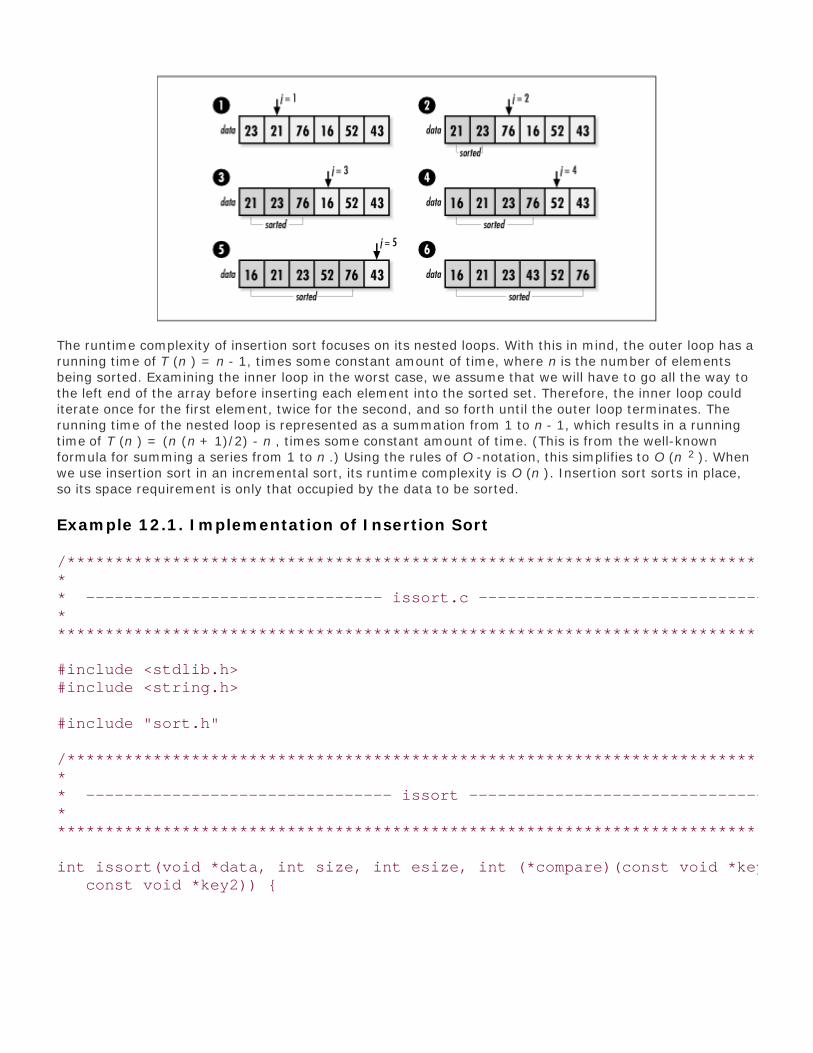
The runtime complexity of insertion sort focuses on its nested loops. With this in mind, the outer loop has arunning time of T (n ) = n - 1, times some constant amount of time, where n is the number of elementsbeing sorted. Examining the inner loop in the worst case, we assume that we will have to go all the way tothe left end of the array before inserting each element into the sorted set. Therefore, the inner loop coulditerate once for the first element, twice for the second, and so forth until the outer loop terminates. Therunning time of the nested loop is represented as a summation from 1 to n - 1, which results in a runningtime of T (n ) = (n (n + 1)/2) - n , times some constant amount of time. (This is from the well-knownformula for summing a series from 1 to n .) Using the rules of O -notation, this simplifies to O (n 2 ). Whenwe use insertion sort in an incremental sort, its runtime complexity is O (n ). Insertion sort sorts in place,so its space requirement is only that occupied by the data to be sorted.
Example 12.1. Implementation of Insertion Sort
/****************************************************************************** ** ------------------------------- issort.c ------------------------------- ** ******************************************************************************/
#include <stdlib.h>#include <string.h>
#include "sort.h"
/****************************************************************************** ** -------------------------------- issort -------------------------------- ** ******************************************************************************/
int issort(void *data, int size, int esize, int (*compare)(const void *key1, const void *key2)) {

char *a = data;
void *key;
int i, j;
/****************************************************************************** ** Allocate storage for the key element. ** ******************************************************************************/
if ((key = (char *)malloc(esize)) == NULL) return -1;
/****************************************************************************** ** Repeatedly insert a key element among the sorted elements. ** ******************************************************************************/
for (j = 1; j < size; j++) {
memcpy(key, &a[j * esize], esize); i = j - 1;
/************************************************************************** * * * Determine the position at which to insert the key element. * * * **************************************************************************/
while (i >= 0 && compare(&a[i * esize], key) > 0) {
memcpy(&a[(i + 1) * esize], &a[i * esize], esize); i--;
}
memcpy(&a[(i + 1) * esize], key, esize);
}
/****************************************************************************** *

* Free the storage allocated for sorting. ** ******************************************************************************/
free(key);
return 0;
}
Top

Mastering Algorithms with CBy Kyle Loudon
Slots : 1
Table of Contents
Chapter 12. Sorting and Searching
Content
12.4 Description of Quicksort
Quicksort is a divide-and-conquer sorting algorithm (see Chapter 1). It is widely regarded as the bestfor general use. Like insertion sort, it is a comparison sort that sorts in place, but its efficiency makesit a better choice for medium to large sets of data.
Returning to the example of sorting a pile of canceled checks by hand, we begin with an unsorted pilethat we partition in two. In one pile we place all checks numbered less than or equal to what we thinkmay be the median value, and in the other pile we place the checks greater than this. Once we havethe two piles, we divide each of them in the same manner, and we repeat the process until we endup with one check in every pile. At this point, the checks are sorted.
Since quicksort is a divide-and-conquer algorithm, it is helpful to consider it more formally in terms ofthe three steps common to all divide-and-conquer algorithms:
Divide: partition the data into two partitions around a partition value.1.Conquer: sort the two partitions by recursively applying quicksort to them.2.Combine: do nothing since the partitions are sorted after the previous step.3.
Considering its popularity, it may be surprising that the worst case of quicksort is no better than theworst case of insertion sort. However, with a little care we can make the worst case of quicksort sounlikely that we can actually count on the algorithm performing to its average case, which isconsiderably better. The key to reliably achieving quicksort's average-case performance lies in howwe choose the partition value in the divide step.
Quicksort performs badly when we choose partition values that continually force the majority of theelements into one partition. Instead, we need to partition the elements in as balanced a manner aspossible. For example, partitioning around 10 in the set {15, 20, 18, 51, 36, 10, 77, 43} results inthe unbalanced partitions of {10} and {20, 18, 51, 36, 15, 77, 43}. On the other hand, partitioningaround 36 results in the more balanced partitions of {15, 20, 18, 10} and {36, 51, 77, 43}.
One approach that works well in choosing partition values is to select them randomly. Statistically,this prevents any particular set of data from eliciting bad behavior, even if we try to bog down thealgorithm intentionally. We can improve partitioning further by randomly choosing three elementsand selecting their median as the partition value. This is called the median-of-three method, whichvirtually guarantees average-case performance. Because this approach to partitioning relies on thestatistical properties of random numbers to help the performance of quicksort overall, quicksort is agood example of a randomized algorithm (see Chapter 1).

Top

Mastering Algorithms with CBy Kyle LoudonSlots : 1Table of ContentsChapter 12. Sorting and Searching
Content
12.5 Interface for Quicksortqksort
int qksort(void *data, int size, int esize, int i, int k, int (*compare) (const void *key1, const void *key2));
Return Value
0 if sorting is successful, or -1 otherwise.
Description
Uses quicksort to sort the array of elements in data . The number of elements in data is specified by
size . The size of each element is specified by esize . The arguments i and k define the current
partition being sorted and initially should be and size - 1, respectively. The function pointer comparespecifies a user-defined function to compare elements. It should perform in a manner similar to that
described for issort . When qksort returns, data contains the sorted elements.
Complexity
O (n lg n ), where n is the number of elements to be sorted.
Top

Mastering Algorithms with CBy Kyle LoudonSlots : 1Table of ContentsChapter 12. Sorting and Searching
Content
12.6 Implementation and Analysis of Quicksort
Quicksort works fundamentally by recursively partitioning an unsorted set of elements until all partitions
contain a single element. In the implementation presented here, data initially contains the unsorted set
of size elements stored in a single block of contiguous storage. Quicksort sorts in place, so all
partitioning is performed in data as well. When qksort returns, data is completely sorted.
As we have seen, an important part of quicksort is how we partition the data. This task is performed in the
function partition (see Example 12.2 ) . This function partitions the elements between positions i and k in
data , where i is less than k .
We begin by selecting a partition value using the median-of-three method mentioned earlier. Once the
partition value has been selected, we move from k to the left in data until we find an element that is
less than or equal to it. This element belongs in the left partition. Next, we move from i to the right until
we find an element that is greater than or equal to the partition value. This element belongs in the rightpartition. Once two elements are found in the wrong partition, they are swapped. We continue in this way
until i and k cross. (You may want to consider how we know that if any one element is in the wrong
partition, there is always one that can be swapped with it.) Once i and k cross, all elements to the left of
the partition value are less than or equal to it, and all elements to the right are greater (see Figure 12.2 ).
Figure 12.2. Partitioning around 28

Now we look at how the recursion proceeds in qksort (see Example 12.2 ). On the initial call to qksort , iis set to and k is set to size - 1. We begin by calling partition to partition data between positions iand k . When partition returns, j is assigned the position of the element that defines where the elements
between i and k are partitioned. Next, we call qksort recursively for the left partition, which is from
position i to j . Sorting left partitions continues recursively until an activation of qksort is passed a
partition containing a single element. In this activation, i will not be less than k , so the call terminates.
In the previous activation of qksort , this causes an iteration to the right partition, from position j + 1 to k. Overall, we continue in this way until the first activation of qksort terminates, at which point the data iscompletely sorted (see Figure 12.3 ).
The analysis of quicksort centers around its average-case performance, which is widely accepted as itsmetric. Even though the worst case of quicksort is no better than that of insertion sort, O (n 2 ), quicksortreliably performs much closer to its average-case running time, O (n lg n ), where n is the number ofelements being sorted.
Figure 12.3. Sorting with quicksort assuming optimal partitioning

Determining the runtime complexity for the average case of quicksort depends on the assumption thatthere will be an even distribution of balanced and unbalanced partitions. This assumption is reasonable ifthe median-of-three method for partitioning is used. In this case, as we repeatedly partition the array, it ishelpful to picture the tree shown in Figure 12.3 , which has a height of (lg n ) + 1. Since for the top lg nlevels of the tree, we must traverse all n elements in order to form the partitions of the next level,quicksort runs in time O (n lg n ). Quicksort sorts in place, so its space requirement is only that occupied bythe data to be sorted.
Example 12.2. Implementation of Quicksort
/****************************************************************************** ** ------------------------------- qksort.c ------------------------------- ** ******************************************************************************/
#include <stdlib.h>#include <string.h>
#include "sort.h"
/****************************************************************************** ** ------------------------------ compare_int ----------------------------- ** ******************************************************************************/
static int compare_int(const void *int1, const void *int2) {
/****************************************************************************** ** Compare two integers (used during median-of-three partitioning). ** ******************************************************************************/
if (*(const int *)int1 > *(const int *)int2) return 1;else if (*(const int *)int1 < *(const int *)int2) return -1;else return 0;
}
/****************************************************************************** ** ------------------------------- partition ------------------------------ *

* ******************************************************************************/
static int partition(void *data, int esize, int i, int k, int (*compare) (const void *key1, const void *key2)) {
char *a = data;
void *pval, *temp;
int r[3];
/****************************************************************************** ** Allocate storage for the partition value and swapping. ** ******************************************************************************/
if ((pval = malloc(esize)) == NULL) return -1;
if ((temp = malloc(esize)) == NULL) {
free(pval); return -1;
}
/****************************************************************************** ** Use the median-of-three method to find the partition value. ** ******************************************************************************/
r[0] = (rand() % (k - i + 1)) + i;r[1] = (rand() % (k - i + 1)) + i;r[2] = (rand() % (k - i + 1)) + i;issort(r, 3, sizeof(int), compare_int);memcpy(pval, &a[r[1] * esize], esize);
/****************************************************************************** ** Create two partitions around the partition value. ** ******************************************************************************/

i--;k++;
while (1) {
/************************************************************************** * * * Move left until an element is found in the wrong partition. * * * **************************************************************************/
do {
k--;
} while (compare(&a[k * esize], pval) > 0);
/************************************************************************** * * * Move right until an element is found in the wrong partition. * * * **************************************************************************/
do {
i++;
} while (compare(&a[i * esize], pval) < 0);
if (i >= k) {
/*********************************************************************** * * * Stop partitioning when the left and right counters cross. * * * ***********************************************************************/
break;
}
else {
/*********************************************************************** * * * Swap the elements now under the left and right counters. *

* * ***********************************************************************/
memcpy(temp, &a[i * esize], esize); memcpy(&a[i * esize], &a[k * esize], esize); memcpy(&a[k * esize], temp, esize);
}
}
/****************************************************************************** ** Free the storage allocated for partitioning. ** ******************************************************************************/
free(pval);free(temp);
/****************************************************************************** ** Return the position dividing the two partitions. ** ******************************************************************************/
return k;
}
/****************************************************************************** ** -------------------------------- qksort -------------------------------- ** ******************************************************************************/
int qksort(void *data, int size, int esize, int i, int k, int (*compare) (const void *key1, const void *key2)) {
int j;
/****************************************************************************** ** Stop the recursion when it is not possible to partition further. ** ******************************************************************************/

while (i < k) {
/************************************************************************** * * * Determine where to partition the elements. * * * **************************************************************************/
if ((j = partition(data, esize, i, k, compare)) < 0) return -1;
/************************************************************************** * * * Recursively sort the left partition. * * * **************************************************************************/
if (qksort(data, size, esize, i, j, compare) < 0) return -1;
/************************************************************************** * * * Iterate and sort the right partition. * * * **************************************************************************/
i = j + 1;
}
return 0;
}
Top

Mastering Algorithms with CBy Kyle LoudonSlots : 1Table of ContentsChapter 12. Sorting and Searching
Content
12.7 Quicksort Example: Directory Listings
In a hierarchical file system , files are typically organized conceptually into directories. For any directory, wemay want to see a list of the files and subdirectories the directory contains. In Unix, we do this with the lscommand, for example. At the command prompt in Windows, we do this with the dir command.
This section presents a function called directls , which implements the same basic functionality that ls
provides. It uses the system call readdir to create a listing of the directory specified in path (see
Examples Example 12.3 and Example 12.4 ). Just as ls does in the default case, directls sorts the listing byname. Because we allocate the listing using realloc as we build it, it is the responsibility of the caller to freeit with free once it is no longer needed.
The runtime complexity of directls is O (n lg n ), where n is the number of entries in the directory beinglisted. This is because retrieving n directory entries is an operation that runs in O (n ) time overall, whilethe subsequent call to qksort sorts the entries in O (n lg n ) time.
Example 12.3. Header for Getting Directory Listings
/****************************************************************************** ** ------------------------------ directls.h ------------------------------ ** ******************************************************************************/
#ifndef DIRECTLS_H#define DIRECTLS_H
#include <dirent.h>
/****************************************************************************** *

* Define a structure for directory entries. ** ******************************************************************************/
typedef struct Directory_ {
char name[MAXNAMLEN + 1];
} Directory;
/****************************************************************************** ** --------------------------- Public Interface --------------------------- ** ******************************************************************************/
int directory(const char *path, Directory **dir);
#endif
Example 12.4. Implementation of a Function for Getting Directory Listings
/****************************************************************************** ** ------------------------------ directls.c ------------------------------ ** ******************************************************************************/
#include <dirent.h>#include <stdio.h>#include <stdlib.h>#include <string.h>
#include "directls.h"#include "sort.h"
/****************************************************************************** ** ------------------------------ compare_dir ----------------------------- ** ******************************************************************************/
static int compare_dir(const void *key1, const void *key2) {
int retval;

if ((retval = strcmp(((const Directory *)key1)->name, ((const Directory *) key2)->name)) > 0) return 1;else if (retval < 0) return -1;else return 0;
}
/****************************************************************************** ** ------------------------------- directls ------------------------------ ** ******************************************************************************/
int directls(const char *path, Directory **dir) {
DIR *dirptr;
Directory *temp;
struct dirent *curdir;
int count, i;
/****************************************************************************** ** Open the directory. ** ******************************************************************************/
if ((dirptr = opendir(path)) == NULL) return -1;
/****************************************************************************** ** Get the directory entries. ** ******************************************************************************/
*dir = NULL;count = 0;
while ((curdir = readdir(dirptr)) != NULL) {

count++;
if ((temp = (Directory *)realloc(*dir, count * sizeof(Directory))) == NULL) {
free(*dir); return -1;
}
else {
*dir = temp;
}
strcpy(((*dir)[count - 1]).name, curdir->d_name);
}
closedir(dirptr);
/****************************************************************************** ** Sort the directory entries by name. ** ******************************************************************************/
if (qksort(*dir, count, sizeof(Directory), 0, count - 1, compare_dir) != 0) return -1;
/****************************************************************************** ** Return the number of directory entries. ** ******************************************************************************/
return count;
}
Top

Mastering Algorithms with CBy Kyle Loudon
Slots : 1
Table of Contents
Chapter 12. Sorting and Searching
Content
12.8 Description of Merge Sort
Merge sort is another example of a divide-and-conquer sorting algorithm (see Chapter 1). Likequicksort, it relies on making comparisons between elements to sort them. However, it does not sortin place.
Returning once again to the example of sorting a pile of canceled checks by hand, we begin with anunsorted pile that we divide in half. Next, we divide each of the resulting two piles in half andcontinue this process until we end up with one check in every pile. Once all piles contain a singlecheck, we merge the piles two by two so that each new pile is a sorted combination of the two thatwere merged. Merging continues until we end up with one big pile again. At this point, the checks aresorted.
As with quicksort, since merge sort is a divide-and-conquer algorithm, it is helpful to consider it moreformally in terms of the three steps common to all divide-and-conquer algorithms:
Divide: we divide the data in half.1.Conquer: we sort the two divisions by recursively applying merge sort to them.2.Combine: we merge the two divisions into a single sorted set.3.
The distinguishing component of merge sort is its merging process. This is the process that takes twosorted sets and merges them into a single sorted one. As we will see, merging two sorted sets isefficient because we need only make one pass through each set. This fact, combined with thepredictable way the algorithm divides the data, makes merge sort in all cases as good as the averagecase of quicksort.
Unfortunately, the space requirement of merge sort presents a drawback. Because merging cannotbe performed in place, merge sort requires twice the space of the unsorted data. This significantlyreduces its desirability in the general case since we can expect to sort just as fast using quicksort,without the extra storage requirement. However, merge sort is nevertheless valuable for very largesets of data because it divides the data in predictable ways. This allows us to divide the data intomore manageable pieces ourselves, use merge sort to sort them, and then perform as many mergesas necessary without having to keep the entire set of data in memory all at once.
Top

Mastering Algorithms with CBy Kyle LoudonSlots : 1Table of ContentsChapter 12. Sorting and Searching
Content
12.9 Interface for Merge Sortmgsort
int mgsort(void *data, int size, int esize, int i, int k, int (*compare) (const void *key1, const void *key2));
Return Value
0 if sorting is successful, or -1 otherwise.
Description
Uses merge sort to sort the array of elements in data . The number of elements in data is specified by
size . The size of each element is specified by esize . The arguments i and k define the current
division being sorted and initially should be and size - 1, respectively. The function pointer comparespecifies a user-defined function to compare elements. It should perform in a manner similar to that
described for issort . When mgsort returns, data contains the sorted elements.
Complexity
O (n lg n ), where n is the number of elements to be sorted.
Top

Mastering Algorithms with CBy Kyle LoudonSlots : 1Table of ContentsChapter 12. Sorting and Searching
Content
12.10 Implementation and Analysis of Merge Sort
Merge sort works fundamentally by recursively dividing an unsorted set of elements into single-elementdivisions and merging the divisions repeatedly until a single set is reproduced. In the implementation
presented here, data initially contains the unsorted set of size elements stored in a single block of
contiguous storage. Since merging is not performed in place, mgsort allocates additional storage for the
merges. Before mgsort returns, the final merged set is copied back into data .
As we have seen, an important part of merge sort is the process of merging two sorted sets into a singlesorted one. This task is performed by the function merge (see Example 12.5 ), which merges the sets
defined from position i to j and from j + 1 to k in data into a single sorted one from i to k .
Initially, ipos and jpos point to the beginning of each sorted set. Merging continues as long as there
are still elements in at least one of the sets. While this is true, we proceed as follows. If one set has noelements remaining to be merged, we place all elements remaining in the other set into the merged set.Otherwise, we look at which set contains the next element that should be placed in the merged set to keep
it properly ordered, place that element in the merged set, and increment ipos or jpos to the next
element depending on from which set the element came (see Figure 12.4 ).
Figure 12.4. Merging two sorted sets

Now we look at how the recursion proceeds in mgsort (see Example 12.5 ). On the initial call to mgsort , iis set to and k is set to size - 1. We begin by dividing data so that j is set to the position of the
middle element. Next, we call mgsort for the left division, which is from position i to j . We continue
dividing left divisions recursively until an activation of mgsort is passed a division containing a single
element. In this activation, i will not be less than k , so the call terminates. In the previous activation of
mgsort , this causes mgsort to be invoked on the right division of the data, from position j + 1 to k .
Once this call returns, we merge the two sets. Overall, we continue in this way until the last activation ofmgsort performs its merge, at which point the data is completely sorted (see Figure 12.5 ).
Figure 12.5. Sorting with merge sort

An analysis of merge sort is simplified when we realize that the algorithm is very predictable. If we divide aset of data repeatedly in half as shown in Figure 12.5 , lg n levels of divisions are required before all setscontain one element, where n is the number of elements being sorted. For two sorted sets of p and qelements, merging runs in O (p + q ) time because a single pass must be made through each set toproduce a merged one. Since for each of the lg n levels of divisions we end up traversing all n elements tomerge the sets at that level, merge sort runs in time O (n lg n ). Because we cannot merge elements inplace, merge sort requires twice the space occupied by the data to be sorted.
Example 12.5. Implementation of Merge Sort
/****************************************************************************** ** ------------------------------- mgsort.c ------------------------------- ** ******************************************************************************/
#include <stdlib.h>#include <string.h>
#include "sort.h"
/*****************************************************************************

* ** --------------------------------- merge -------------------------------- ** ******************************************************************************/
static int merge(void *data, int esize, int i, int j, int k, int (*compare) (const void *key1, const void *key2)) {
char *a = data, *m;
int ipos, jpos, mpos;
/****************************************************************************** ** Initialize the counters used in merging. ** ******************************************************************************/
ipos = i;jpos = j + 1;mpos = 0;
/****************************************************************************** ** Allocate storage for the merged elements. ** ******************************************************************************/
if ((m = (char *)malloc(esize * ((k - i) + 1))) == NULL) return -1;
/****************************************************************************** ** Continue while either division has elements to merge. ** ******************************************************************************/
while (ipos <= j || jpos <= k) {
if (ipos > j) {
/*********************************************************************** * *

* The left division has no more elements to merge. * * * ***********************************************************************/
while (jpos <= k) {
memcpy(&m[mpos * esize], &a[jpos * esize], esize); jpos++; mpos++;
}
continue;
}
else if (jpos > k) {
/*********************************************************************** * * * The right division has no more elements to merge. * * * ***********************************************************************/
while (ipos <= j) {
memcpy(&m[mpos * esize], &a[ipos * esize], esize); ipos++; mpos++;
}
continue;
}
/************************************************************************** * * * Append the next ordered element to the merged elements. * * * **************************************************************************/
if (compare(&a[ipos * esize], &a[jpos * esize]) < 0) {
memcpy(&m[mpos * esize], &a[ipos * esize], esize); ipos++;

mpos++;
}
else {
memcpy(&m[mpos * esize], &a[jpos * esize], esize); jpos++; mpos++;
}
}
/****************************************************************************** ** Prepare to pass back the merged data. ** ******************************************************************************/
memcpy(&a[i * esize], m, esize * ((k - i) + 1));
/****************************************************************************** ** Free the storage allocated for merging. ** ******************************************************************************/
free(m);
return 0;
}
/****************************************************************************** ** -------------------------------- mgsort -------------------------------- ** ******************************************************************************/
int mgsort(void *data, int size, int esize, int i, int k, int (*compare) (const void *key1, const void *key2)) {
int j;
/*****************************************************************************

* ** Stop the recursion when no more divisions can be made. ** ******************************************************************************/
if (i < k) {
/************************************************************************** * * * Determine where to divide the elements. * * * **************************************************************************/
j = (int)(((i + k - 1)) / 2);
/************************************************************************** * * * Recursively sort the two divisions. * * * **************************************************************************/
if (mgsort(data, size, esize, i, j, compare) < 0) return -1;
if (mgsort(data, size, esize, j + 1, k, compare) < 0) return -1;
/************************************************************************** * * * Merge the two sorted divisions into a single sorted set. * * * **************************************************************************/
if (merge(data, esize, i, j, k, compare) < 0) return -1;
}
return 0;
}

Top

Mastering Algorithms with CBy Kyle Loudon
Slots : 1
Table of Contents
Chapter 12. Sorting and Searching
Content
12.11 Description of Counting Sort
Counting sort is an efficient, linear-time sorting algorithm that works by counting how many timeseach element of a set occurs to determine how the set should be ordered. By avoiding thecomparisons that have been a part of the sorting methods presented thus far, counting sort improveson the O (n lg n) runtime bound of comparison sorts.
Counting sort does have some limitations. The most significant is that it works only with integers ordata that can be expressed in some integer form. This is because counting sort makes use of anarray of counts indexed by the integer elements themselves to keep track of how many times eachone occurs. For example, if the integer 3 occurs in the data four times, 4 will be stored initially atposition 3 in the array of counts. Also, we must know the largest integer in the set in order toallocate enough space for the counts.
Aside from being fast, an important virtue of counting sort is that it is stable. Stable sorts leaveelements that have equal values in the same order as they appear in the original set. This is animportant attribute in some cases, as we will see with radix sort.
Top

Mastering Algorithms with CBy Kyle Loudon
Slots : 1
Table of Contents
Chapter 12. Sorting and Searching
Content
12.12 Interface for Counting Sort
ctsort
int ctsort(int *data, int size, int k);
Return Value
0 if sorting is successful, or -1 otherwise.
Description
Uses counting sort to sort the array of integers in data. The number of integers in data is specifiedby size. The argument k specifies the maximum integer in data, plus 1. When ctsort returns,data contains the sorted integers.
Complexity
O (n + k), where n is the number of integers to be sorted and k is the maximum integer in theunsorted set, plus 1.
Top

Mastering Algorithms with CBy Kyle LoudonSlots : 1Table of ContentsChapter 12. Sorting and Searching
Content
12.13 Implementation and Analysis of Counting Sort
Counting sort works fundamentally by counting how many times integer elements occur in an unsorted set
to determine how the set should be ordered. In the implementation presented here, data initially contains
the unsorted set of size integer elements stored in a single block of contiguous storage. Additional
storage is allocated to store the sorted data temporarily. Before ctsort returns, the sorted set is copied back
into data .
After allocating storage, we begin by counting the occurrences of each element in data (see Example
12.6 ). These are placed in an array of counts, counts , indexed by the integer elements themselves
(see Figure 12.6 , step 1b). Once the occurrences of each element in data have been counted, we adjust
the counts to reflect the number of elements that will come before each element in the sorted set. We dothis by adding the count of each element in the array to the count of the element that follows it (see Figure
12.6 , step 1c). Effectively, counts then contains the offsets at which each element belongs in the sorted
set, temp .
To complete the sort, we place each element in temp at its designated offset (see Figure 12.6 , steps 2a- f
). The count for each element is decreased by 1 as temp is updated so that integers appearing more than
once in data appear more than once in temp as well.
Figure 12.6. Sorting with counting sort

The runtime complexity of counting sort is O (n + k ), where n is the number of integers in the data and kis the largest integer value in the set being sorted, plus 1. This is because counting sort consists of threeloops, two that run in time proportional to n , and one that runs in time proportional to k . For space,counting sort requires two arrays of size n and an array of size k .
Example 12.6. Implementation of Counting Sort
/****************************************************************************** ** ------------------------------- ctsort.c ------------------------------- *

* ******************************************************************************/
#include <stdlib.h>#include <string.h>
#include "sort.h"
/****************************************************************************** ** -------------------------------- ctsort -------------------------------- ** ******************************************************************************/
int ctsort(int *data, int size, int k) {
int *counts, *temp;
int i, j;
/****************************************************************************** ** Allocate storage for the counts. ** ******************************************************************************/
if ((counts = (int *)malloc(k * sizeof(int))) == NULL) return -1;
/****************************************************************************** ** Allocate storage for the sorted elements. ** ******************************************************************************/
if ((temp = (int *)malloc(size * sizeof(int))) == NULL) return -1;
/****************************************************************************** ** Initialize the counts. ** ******************************************************************************/

for (i = 0; i < k; i++) counts[i] = 0;
/****************************************************************************** ** Count the occurrences of each element. ** ******************************************************************************/
for (j = 0; j < size; j++) counts[data[j]] = counts[data[j]] + 1;
/****************************************************************************** ** Adjust each count to reflect the counts before it. ** ******************************************************************************/
for (i = 1; i < k; i++) counts[i] = counts[i] + counts[i - 1];
/****************************************************************************** ** Use the counts to position each element where it belongs. ** ******************************************************************************/
for (j = size - 1; j >= 0; j--) {
temp[counts[data[j]] - 1] = data[j]; counts[data[j]] = counts[data[j]] - 1;
}
/****************************************************************************** ** Prepare to pass back the sorted data. ** ******************************************************************************/
memcpy(data, temp, size * sizeof(int));
/****************************************************************************** ** Free the storage allocated for sorting. ** *

*****************************************************************************/
free(counts);free(temp);
return 0;
}
Top

Mastering Algorithms with CBy Kyle Loudon
Slots : 1
Table of Contents
Chapter 12. Sorting and Searching
Content
12.14 Description of Radix Sort
Radix sort is another efficient, linear-time sorting algorithm. It works by sorting data in pieces calleddigits, one digit at a time, from the digit in the least significant position to the most significant. Usingradix sort to sort the set of radix-10 numbers {15, 12, 49, 16, 36, 40}, for example, produces {40,12, 15, 16, 36, 49} after sorting on the least significant digit, and {12, 15, 16, 36, 40, 49} aftersorting on the most significant digit.
It is very important that radix sort use a stable sort for sorting on the digit values in each position.This is because once an element has been assigned a place according to the digit value in a lesssignificant position, its place must not change unless sorting on one of the more significant digitsrequires it. For example, in the set given earlier, when 12 and 15 were sorted on the digits in themost significant position, since both integers contained a "1," a nonstable sort may not have leftthem in the order they were placed when sorted by their least significant digit. A stable sort ensuresthat these two are not reordered. Radix sort uses counting sort because, aside from being stable, itruns in linear time, and for any radix, we know the largest integer any digit may be.
Radix sort is not limited to sorting data keyed by integers, as long as we can divide the elements intointeger pieces. For example, we might sort a set of strings as radix-28 values. Or we might sort a setof 64-bit integers as four-digit, radix-216 values. Exactly what value we choose as a radix depends onthe data itself and minimizing pn + pk considering space constraints, where p is the number of digitpositions in each element, n is the number of elements, and k is the radix (the number of possibledigit values in any position). Generally, we try to keep k close to and no more than n.
Top

Mastering Algorithms with CBy Kyle Loudon
Slots : 1
Table of Contents
Chapter 12. Sorting and Searching
Content
12.15 Interface for Radix Sort
rxsort
int rxsort(int *data, int size, int p, int k);
Return Value
0 if sorting is successful, or -1 otherwise.
Description
Uses radix sort to sort the array of integers in data. The number of integers in data is specified bysize. The argument p specifies the number of digit positions in each integer. The argument kspecifies the radix. When rxsort returns, data contains the sorted integers.
Complexity
O (pn + pk), where n is the number of integers to be sorted, k is the radix, and p is the number ofdigit positions.
Top

Mastering Algorithms with CBy Kyle LoudonSlots : 1Table of ContentsChapter 12. Sorting and Searching
Content
12.16 Implementation and Analysis of Radix Sort
Radix sort works fundamentally by applying counting sort one position at a time to a set of data. In the
implementation presented here, data initially contains the unsorted set of size integer elements stored
in a single block of contiguous storage. When rxsort returns, data is completely sorted.
If we understand counting sort, the operation of radix sort is simple. A single loop governs the position onwhich we are currently sorting (see Example 12.7 ). Position by position, we apply counting sort to shuffleand reshuffle the elements, beginning with the least significant position. Once we have shuffled theelements by the digits in the most significant position, sorting is complete (see Figure 12.7 ). A simpleapproach involving exponentiation and modular arithmetic is used to obtain each digit value. This workswell for integers. Different types of data require different approaches. Some approaches may requireconsidering machine-specific details, such as byte ordering and word alignment.
Figure 12.7. Sorting integers as radix-10 numbers with radix sort
Not surprisingly, the runtime complexity of radix sort depends on the stable sorting algorithm chosen tosort the digits. Because radix sort applies counting sort once for each of the p positions of digits in the data,

radix sort runs in p times the runtime complexity of counting sort, or O (pn + pk ). Its space requirement isthe same as for counting sort: two arrays of size n and an array of size k .
Example 12.7. Implementation of Radix Sort
/****************************************************************************** ** ------------------------------- rxsort.c ------------------------------- ** ******************************************************************************/
#include <limits.h>#include <math.h>#include <stdlib.h>#include <string.h>
#include "sort.h"
/****************************************************************************** ** -------------------------------- rxsort -------------------------------- ** ******************************************************************************/
int rxsort(int *data, int size, int p, int k) {
int *counts, *temp;
int index, pval, i, j, n;
/****************************************************************************** ** Allocate storage for the counts. ** ******************************************************************************/
if ((counts = (int *)malloc(k * sizeof(int))) == NULL) return -1;
/****************************************************************************** *

* Allocate storage for the sorted elements. ** ******************************************************************************/
if ((temp = (int *)malloc(size * sizeof(int))) == NULL) return -1;
/****************************************************************************** ** Sort from the least significant position to the most significant. ** ******************************************************************************/
for (n = 0; n < p; n++) {
/************************************************************************** * * * Initialize the counts. * * * **************************************************************************/
for (i = 0; i < k; i++) counts[i] = 0;
/************************************************************************** * * * Calculate the position value. * * * **************************************************************************/
pval = (int)pow((double)k, (double)n);
/************************************************************************** * * * Count the occurrences of each digit value. * * * **************************************************************************/
for (j = 0; j < size; j++) {
index = (int)(data[j] / pval) % k; counts[index] = counts[index] + 1;
}
/**************************************************************************

* * * Adjust each count to reflect the counts before it. * * * **************************************************************************/
for (i = 1; i < k; i++) counts[i] = counts[i] + counts[i - 1];
/************************************************************************** * * * Use the counts to position each element where it belongs. * * * **************************************************************************/
for (j = size - 1; j >= 0; j--) {
index = (int)(data[j] / pval) % k; temp[counts[index] - 1] = data[j]; counts[index] = counts[index] - 1;
}
/************************************************************************** * * * Prepare to pass back the data as sorted thus far. * * * **************************************************************************/
memcpy(data, temp, size * sizeof(int));
}
/****************************************************************************** ** Free the storage allocated for sorting. ** ******************************************************************************/
free(counts);free(temp);
return 0;
}

Top

Mastering Algorithms with CBy Kyle Loudon
Slots : 1
Table of Contents
Chapter 12. Sorting and Searching
Content
12.17 Description of Binary Search
Binary search is a technique for searching that works similarly to how we might systematically guessnumbers in a guessing game. For example, suppose someone tells us to guess a number betweenand 99. The consistently best approach is to begin with 49, the number in the middle of and 99. If 49is too high, we try 24, the number in the middle of the lower half of to 99 (0 to 48). Otherwise, if 49is too low, we try 74, the number in the middle of the upper half of to 99 (50 to 99). We repeat thisprocess for each narrowed range until we guess right.
Binary search begins with a set of data that is sorted. To start the search, we inspect the middleelement of the sorted set. If the element is greater than the one we are looking for, we let the lowerhalf of the set be the new set to search. Otherwise, if the element is less, we let the upper half be thenew set. We repeat this process on each smaller set until we either locate the element we are lookingfor or cannot divide the set any further.
Binary search works with any type of data provided we can establish an ordering among theelements. It is a simple algorithm, but as you might suspect, its reliance on sorted data makes itinefficient for sets in which there are frequent insertions and deletions. This is because for eachinsertion or deletion, we must ensure that the set stays sorted for the search to work properly.Keeping a set sorted is expensive relative to searching it. Also, elements must be in contiguousstorage. Thus, binary search is best utilized when the set to be searched is relatively static.
Top

Mastering Algorithms with CBy Kyle Loudon
Slots : 1
Table of Contents
Chapter 12. Sorting and Searching
Content
12.18 Interface for Binary Search
bisearch
int bisearch(void *sorted, void *target, int size, int esize, int (*compare)(const void *key1, const void *key2);
Return Value
Index of the target if found, or -1 otherwise.
Description
Uses binary search to locate target in sorted, a sorted array of elements. The number ofelements in sorted is specified by size. The size of each element is specified by esize. Thefunction pointer compare specifies a user-defined function to compare elements. This functionshould return 1 if key1 > key2, if key1 = key2, and -1 if key1 < key2.
Complexity
O (lg n), where n is the number of elements to be searched.
Top

Mastering Algorithms with CBy Kyle LoudonSlots : 1Table of ContentsChapter 12. Sorting and Searching
Content
12.19 Implementation and Analysis of Binary Search
Binary search works fundamentally by dividing a sorted set of data repeatedly and inspecting the elementin the middle of each division. In the implementation presented here, the sorted set of data resides in
sorted , a single block of contiguous storage. The argument target is the data we are searching for.
This implementation revolves around a single loop controlled by the variables left and right , which
define the boundaries of the current set in which we are focusing our search (see Example 12.8 ). Initially,
we set left and right to and size - 1, respectively. During each iteration of the loop, we set
middle to the middle element of the set defined by left and right . If the element at middle is
less than the target, we move the left index to one element after middle . Thus, the next set searched is
the upper half of the current set. If the element at middle is greater than the target, we move the right
index to one element before middle . Thus, the next set searched is the lower half of the current set. As
the search continues, left moves from left to right, and right moves from right to left. The search
terminates once we encounter the target at middle , or when left and right cross, if the target is
not found. Figure 12.8 illustrates this process.
Figure 12.8. Searching for 47 using binary search

The runtime complexity of binary search depends on the maximum number of divisions possible during thesearching process. For a set of n elements, we can perform up to lg n divisions. For binary search, thisrepresents the number of inspections that we could end up performing in the worst case: when the target isnot found, for example. Therefore, the runtime complexity of binary search is O (lg n ).
Example 12.8. Implementation of Binary Search
/****************************************************************************** ** ------------------------------ bisearch.c ------------------------------ ** ******************************************************************************/
#include <stdlib.h>#include <string.h>
#include "search.h"
/****************************************************************************** *

* ------------------------------- bisearch ------------------------------- ** ******************************************************************************/
int bisearch(void *sorted, const void *target, int size, int esize, int (*compare)(const void *key1, const void *key2)) {
int left, middle, right;
/****************************************************************************** ** Continue searching until the left and right indices cross. ** ******************************************************************************/
left = 0;right = size - 1;
while (left <= right) {
middle = (left + right) / 2;
switch (compare(((char *)sorted + (esize * middle)), target)) {
case -1:
/*********************************************************************** * * * Prepare to search to the right of the middle index. * * * ***********************************************************************/
left = middle + 1; break;
case 1:
/*********************************************************************** * * * Prepare to search to the left of the middle index. * * * ***********************************************************************/
right = middle - 1;

break;
case 0:
/*********************************************************************** * * * Return the exact index where the data has been found. * * * ***********************************************************************/
return middle;
}
}
/****************************************************************************** ** Return that the data was not found. ** ******************************************************************************/
return -1;
}
Top

Mastering Algorithms with CBy Kyle LoudonSlots : 1Table of ContentsChapter 12. Sorting and Searching
Content
12.20 Binary Search Example: Spell Checking
Using spell checkers has become an expected part of preparing all types of documents. From a computingstandpoint, a basic spell checker works simply by checking words in a string of text against a dictionary.The dictionary contains the set of acceptable words.
The example presented here consists of a function, spell (see Examples Example 12.9 and Example 12.10 ),that checks the spelling of words from a string of text one word at a time. The function accepts three
arguments: dictionary is a sorted array of acceptable strings, size is the number of strings in the
dictionary, and word is the word to check. The function calls bisearch to look up word in dictionary. If it finds the word, it is spelled correctly.
The runtime complexity of spell is O (lg n ), the same time as bisearch , where n is the number of words in
dictionary . The runtime complexity of checking an entire document is O (m lg n ), where m is the
number of words in the text to validate and n is the number of words in the dictionary.
Example 12.9. Header for Spell Checking
/****************************************************************************** ** -------------------------------- spell.h ------------------------------- ** ******************************************************************************/
#ifndef SPELL_H#define SPELL_H
/****************************************************************************** ** Define the maximum size for words in the dictionary. *

* ******************************************************************************/
#define SPELL_SIZE 31
/****************************************************************************** ** --------------------------- Public Interface --------------------------- ** ******************************************************************************/
int spell(char (*dictionary)[SPELL_SIZE], int size, const char *word);
#endif
Example 12.10. Implementation of a Function for Spell Checking
/****************************************************************************** ** -------------------------------- spell.c ------------------------------- ** ******************************************************************************/
#include <string.h>
#include "search.h"#include "spell.h"
/****************************************************************************** ** ------------------------------ compare_str ----------------------------- ** ******************************************************************************/
static int compare_str(const void *str1, const void *str2) {
int retval;
if ((retval = strcmp((const char *)str1, (const char *)str2)) > 0) return 1;else if (retval < 0) return -1;else return 0;
}

/****************************************************************************** ** --------------------------------- spell -------------------------------- ** ******************************************************************************/
int spell(char (*dictionary)[SPELL_SIZE], int size, const char *word) {
/****************************************************************************** ** Look up the word. ** ******************************************************************************/
if (bisearch(dictionary, word, size, SPELL_SIZE, compare_str) >= 0) return 1;else return 0;
}
Top

Mastering Algorithms with CBy Kyle LoudonSlots : 1Table of ContentsChapter 12. Sorting and Searching
Content
12.21 Questions and Answers
Q: Suppose we need to sort all of the customer records for a worldwide investment firm by name. The datais so large it cannot be fit into memory all at once. Which sorting algorithm should we use?
A: Merge sort. Aside from running efficiently in O (n lg n ) time, the predictable way that merge sort dividesand merges the data lets us easily manage the data ourselves to efficiently bring it in and out of secondarystorage.
Q: Suppose we are maintaining a list of sorted elements in a user interface. The list is relatively small andthe elements are being entered by a user one at a time. Which sorting algorithm should we use?
A: Insertion sort. The runtime complexity of insertion sort when inserting a single element into a list that isalready sorted is O (n ).
Q: Suppose we need to sort 10 million 80-character strings representing DNA information from a biologicalstudy. Which sorting algorithm should we use?
A: Radix sort. However, precisely how radix sort performs in relation to other sorting algorithms dependson the radix value we choose and our space constraints. An important consideration in selecting radix sortis that the elements in the data are a fixed size and can be broken into integer pieces.
Q: Suppose we need to sort 10,000 C structures containing information about the flight schedule for anairline. Which sorting algorithm should we use?
A: Quicksort. It is the best general-case sorting algorithm and is excellent for medium to large sets of data.
Q: Recall that the interfaces to qksort and mgsort require that i and k be passed by the caller. Why is
this, and how could we avoid it in practice?
A: The arguments i and k are necessary to define smaller and smaller subsets of the data while
recursing. An alternative to the caller providing these is to place each function in a wrapper . Wrappersgenerally provide cleaner public interfaces to functions that are otherwise cumbersome to call directly.

Wrapping qksort , for example, gives us the opportunity to alleviate making the caller pass i and k ,
since we know that initially these always should be set to and size - 1. Wrapping qksort also gives us the
opportunity to encapsulate a call to srand , which seeds the random number generator and prevents certaininputs from consistently eliciting bad behavior. This is something like what the standard library functionqsort actually does. A wrapper might be implemented for qksort in Unix as shown below:
#include <unistd.h>#include <stdlib.h>
#include "sort.h"
int qsrt(void *data, int size, int esize, int (*compare)(const void *key1, const void *key2)) {
srand(getpid());
return qksort(data, size, esize, 0, size - 1, compare);
}
Q: In rxsort , recall that counting sort is implemented explicitly rather than by calling ctsort . Why mightthis have been done?
A: Because radix sort works by considering only a single digit of the elements at a time, our counting sortimplementation would have had to accept additional parameters to tell it which digit to consider as well ashow to obtain each digit value. Recall that modular arithmetic was used in the implementation presented inthis chapter, but other techniques might be more appropriate for some data. For example, for long stringswe might choose to offset two bytes at a time into the string to form digits. Accounting for theseapplication-specific considerations in counting sort would have complicated it substantially. Therefore, aslightly modified form of counting sort was included in the radix sort implementation.
Q: Suppose we have 220 128-bit elements that we would like to sort. What would be the efficiency ofsorting these using quicksort? What would be the efficiency of sorting these as radix-216 numbers usingradix sort? Which approach would be better? Suppose we have 210 128-bit elements rather than 220
elements. How do quicksort and radix sort compare in this case?
A: Sorting with quicksort requires O (n lg n ) = (220 )(20) = (2.10)(107 ) times some constant amount oftime. Considering the elements as radix-216 numbers, the number of digit positions, p , is 8, and thenumber of possible digit values, k , is 216 . Therefore, sorting with radix sort requires O (pn + pk ) =(8)(220 ) + (8)(216 ) = (8.91)(106 ) times some constant amount of time. If the space requirements ofradix sort are acceptable, radix sort is more than twice as efficient as quicksort. In the second case, sortingwith quicksort requires O (n lg n ) = (210 )(10) = 10,240 times some constant amount of time. Radix sortrequires O (pn + pk ) = (8)(210 ) + (8)(216 ) = 532,480 times some constant amount of time, or 50 timesas much time as quicksort! Here is an example of why k is typically chosen to be close to and no more thann . Had we used a radix of 28 , radix sort would have required O (pn + pk ) = (16)(28 ) + (16)(28 ) = 8160times some constant amount of time, and would have been slightly better than quicksort. However, it isworth noting that the space requirement of radix sort may negate small benefits in time in many cases.
Q: In a sorted set, the successor of some node x is the next largest node after x . For example, in a sortedset containing the keys 24, 39, 41, 55, 87, 92, the successor of 41 is 55. How do we find the successor ofan element x using binary search? What is the runtime complexity of this operation?

A: In a sorted set, to determine the successor of some element x using binary search, first we locate x .Next, we simply move one element to the right. The runtime complexity of locating either x or its successoris O (lg n ).
Top

Mastering Algorithms with CBy Kyle Loudon
Slots : 1
Table of Contents
Chapter 12. Sorting and Searching
Content
12.22 Related Topics
Bubble sort
An inefficient O (n2) sorting algorithm that works by exchanging neighboring elements topropagate one element at a time to its correct position in the sorted set.
Tournament sort
An O (n lg n) algorithm that requires three times the space of the data. It works by pairing upelements to promote a "winner" as the next element to be placed in the sorted set.
Heapsort
An efficient sorting algorithm that uses a heap (see Chapter 10) to build a sorted set. Heapsortruns in O (n lg n) and sorts in place. However, a good implementation of quicksort generallybeats it by a small constant factor.
Introsort
A sorting algorithm that behaves like quicksort, but detects when it would be better to switchto heapsort. By doing this, in some cases it gains a slight performance advantage overquicksort.
Bucket sort
A linear-time sorting algorithm on average for data that is uniformly randomly distributed. Itworks by distributing the data into several buckets and sorting the buckets to produce a sortedset.
Top

Mastering Algorithms with CBy Kyle Loudon
Slots : 1
Table of Contents
Part III: Algorithms
Content
Chapter 13. Numerical MethodsNumerical methods are algorithms in numerical analysis. Numerical analysis is the study of problemsin which numbers and approximation play an especially significant role. Computers are particularlywell-suited to problems in numerical analysis because many such problems, while essentiallyinvolving common mathematical operations, require a lot of them. In the early days of computing,scientists monopolized computers with problems like this, which were far too intensive to be carriedout by hand. Even today, problems in numerical analysis still occupy a good part of the cycles ofsome of the largest computers in the world. Hence, numerical analysis is a vast subject, and manynumerical methods are as complicated and specific as the mathematical problems they solve. Thischapter presents three numerical methods that are relatively simple but applicable to a wide varietyof problems.This chapter covers:
Polynomial interpolation
A method of approximating values of a function for which values are known at only a fewpoints. Fundamental to this method is the construction of an interpolating polynomial pn(z) of
degree n, where n + 1 is the number of points for which values are known.Least-squares estimation
A method of determining estimators b1 and b0 for a function y (x) = b1x + b0 so that y (x) is abest-fit line through a set of n points (x0, y0), . . ., (xn - 1, yn - 1). A best-fit line using least-squares estimation minimizes the sum of squared vertical distances between each point (xi , yi), i = 0, . . ., n - 1, and a corresponding point (xi , y (xi ) ) along y (x).
Solution of equations
The process of finding roots of equations having the form f (x) = 0. Whereas for someequations it is possible to determine exact roots, a great deal of the time a method ofapproximation must be used.
Some applications of numerical methods are:
Linear regression models
Statistical models in which there is a linear-form relationship between an independent variablex and a variable y that depends on it. Least-squares estimators help to predict values of y forvalues of x we have not observed experimentally.
Curve fitting

The process of fitting a curve to a number of points. If the points for which we have values arelocated at meaningful places on the curve we are trying to fit, and we know values at enoughpoints, interpolation helps us draw a smooth curve.
Scatter plots
Statistical tools that help ascertain the relationship between an independent variable x and avariable y that depends on it. Using least-squares estimators to draw a best-fit line through alinear-form scatter plot helps with this.
Approximating functions
The process of determining the value of a function at points for which exact values are notknown. This can be done by constructing an interpolating polynomial of the appropriate degree.
Function tables
Tables containing values of computationally expensive functions or models of complicatedphysical phenomena. Often it is too costly to compute and store values of a function with thegranularity required at some later time. Thus, we store a limited number of points andinterpolate between them.
Scientific computing
An area in which solving equations is one of the most fundamental problems routinelyperformed.
Top

Mastering Algorithms with CBy Kyle Loudon
Slots : 1
Table of Contents
Chapter 13. Numerical Methods
Content
13.1 Description of Polynomial Interpolation
There are many problems that can be described in terms of a function. However, often this functionis not known, and we must infer what we can about it from only a small number of points. To do this,we interpolate between the points. For example, in Figure 13.1, the known points along f (x) are x0, .. ., x8, shown by circular black dots. Interpolation helps us get a good idea of the value of thefunction at points z0, z1, and z2, shown by white squares. This section presents polynomialinterpolation.
Figure 13.1. Interpolation with nine points to find the value of a functionat other points
Fundamental to polynomial interpolation is the construction of a special polynomial called aninterpolating polynomial. To appreciate the significance of this polynomial, let's look at someprinciples of polynomials in general. First, a polynomial is a function of the form:
p(x) = a0+a1x+a2x2+. . . +anxn
where a0, . . ., an are coefficients. Polynomials of this form are said to have degree n, provided an isnonzero. This is the power form of a polynomial, which is especially common in mathematicaldiscussions. However, other forms of polynomials are more convenient in certain contexts. Forexample, a form particularly relevant to polynomial interpolation is the Newton form:

p(x) = a0+a1(x-c1)+a2(x-c1)(x-c2)+ . . . +an(x-c1)(x-c2). . . (x-cn)
where a0, . . ., an are coefficients and c1, . . ., cn are centers. Notice how when c1, . . ., cn are all 0,the Newton form of a polynomial reduces to the power form above.
13.1.1 Constructing an Interpolating Polynomial
Now that we understand a bit about polynomials, let's look at how to construct the polynomial that
interpolates a function f (x). To interpolate f (x), a polynomial pn(z) of degree n is constructedusing n + 1 points, x0, . . ., xn, known along f (x). The points x0, . . ., xn are called interpolationpoints. Using pn(z), we approximate the value of f (x) at x=z. Interpolation requires that point z beon the interval [x0, xn]. pn(z) is constructed using the formula:
where x0, . . ., xn are the points along f (x) for which values are known, and f [ x0], . . ., f [x0, . . .,xn] are divided differences, which are derived from x0, . . ., xn and the values of f (x) at thesepoints. This is called the Newton formula for interpolating polynomials. Notice its similarities with theNewton form of polynomials in general. Divided differences are computed using the formula:
Notice that this formula shows that for divided differences when i < j we must have computed otherdivided differences beforehand. For example, to compute f [x0, x1, x2, x3], values are required for f[x1, x2, x3] and f [x0, x1, x2] in the numerator. Fortunately, we can use a divided-difference table tohelp compute divided differences in a systematic manner (see Figure 13.2).
A divided-difference table consists of several rows. The top row stores x0, . . ., xn. The second rowstores values for f [x0], . . ., f [xn]. To compute each divided difference in the remainder of the table,we draw a diagonal from each divided difference back to f [xi ] and f [xj ] (shown as dotted lines for f[x1, x2, x3] in Figure 13.2). To get xi and xj in the denominator, we then proceed straight up from f[xi ] and f [xj ]. The two divided differences in the numerator are those immediately above the onebeing computed. When the table is complete, the coefficients for the interpolating polynomial are thedivided differences at the far left of each row, beginning with the second row (shown in light gray inFigure 13.2).
Figure 13.2. A divided-difference table for determining the coefficients ofan interpolating polynomial of degree 3

13.1.2 Evaluating an Interpolating Polynomial
Once we have determined the coefficients of the interpolating polynomial pn(z), we evaluate thepolynomial once for each point at which we would like to know the value of f. For example, say weknow the values of f at four points: x0 = -3.0, f (x0) = -5.0; x1 = -2.0, f (x1) = -1.1; x2 = 2.0, f (x2)= 1.9; and x3 = 3.0, f (x3) = 4.8; and we would like to know the value of f at z0 = -2.5, z1 = 0.0, z2
= 1.0, and z3 = 2.5. Since we know four points along f, the interpolating polynomial will have adegree of 3. Figure 13.3 is the divided-difference table for determining the coefficients of p3(z).
Figure 13.3. A divided-difference table producing the coefficients -5.0,3.9, -0.63, and 0.1767

Once we have obtained the coefficients from the divided-difference table, we construct p3(z) usingthe Newton formula for interpolating polynomials presented earlier. Using the coefficients from Figure13.3, the interpolating polynomial is:
p3(z) = -5.0+3.9(z+3.0)+(-0.63)(z+3.0)(z+2.0)+0.1767(z+3.0)(z+2.0)(z-2.0)
Next, we evaluate this polynomial once at each point z. For example, at z0 = -2.5 we perform thefollowing calculation:
p3(-2.5) = -5.0+3.9(0.5)+(-0.63)(0.5)(-0.5)+0.1767(0.5)(-0.5)(-4.5) = -2.694
The value of f at z1, z2, and z3 is determined in a similar manner. The results are tabulated andplotted in Figure 13.4.
Figure 13.4. Interpolating a function f (x) using the polynomial p3(z)presented in the text

Now that we have an understanding of how to interpolate a function, it is important to brieflymention the subject of error. As with any approximation method, it is important to understand thatan interpolating polynomial usually has some amount of error associated with it. To minimize thiserror, qualitatively speaking, we must construct an interpolating polynomial using enough pointsalong f (x), and ones properly spaced, so that the resulting polynomial gives an accurate impressionof the function's character. Naturally, quantitative methods do exist for bounding the error associatedwith interpolation, but this book will not address them (see the related topics at the end of thechapter).
Top

Mastering Algorithms with CBy Kyle LoudonSlots : 1Table of ContentsChapter 13. Numerical Methods
Content
13.2 Interface for Polynomial Interpolationinterpol
int interpol (const double *x, const double *fx, int n, double *z, double *pz, int m);
Return Value
0 if interpolating is successful, or -1 otherwise.
Description
Determines the value of a function at specified points using polynomial interpolation. Points at which values
are known are specified by the caller in x . The known values of the function at each point in x are
specified in fx . Points at which values are to be determined are specified in z . The values calculated for
the points passed in z are returned in pz . The number of values in x and fx is specified as n . The
number of points in z (and thus returned in pz ) is specified as m . It is the responsibility of the caller to
manage the storage associated with x , fx , z , and pz .
Complexity
O (mn 2 ), where m is the number of values to determine and n is the number of points at which values areknown.
Top

Mastering Algorithms with CBy Kyle LoudonSlots : 1Table of ContentsChapter 13. Numerical Methods
Content
13.3 Implementation and Analysis of Polynomial Interpolation
Polynomial interpolation works fundamentally by determining the value of an interpolating polynomial at anumber of desired points. To obtain this polynomial, first we must determine its coefficients by computingdivided differences.
The interpol operation begins by allocating space for the divided differences as well as for the coefficients tobe determined (see Example 13-1 ). Note that since the entries in each row in a divided-difference tabledepend only on the entries computed in the row before it (see Figure 13.2 and Figure 13.3 ), we do not
have to keep all of the table around at once. Thus, we allocate space only for the largest row, which has nentries. Next, we initialize the first row in the table with the values in fx . This is so that we are ready to
compute what equates to the third row of the divided-difference table. (Nothing needs to be done for the
first two rows because these entries are already stored in x and fx .) The final initialization step is to
store the value of fx[0] in coeff[0] since this is the first coefficient of the interpolating polynomial.
The process of computing divided differences revolves around a single nested loop, which uses the formulafor divided differences discussed earlier in the chapter. In terms of Figure 13.2 and Figure 13.3 , the outer
loop, k , counts the number of rows for which entries must be computed (excluding the rows for x and
fx ). The inner loop, i , controls which entry is being computed in the current row. As we complete the
entries in each row, the value in table [0] becomes the next coefficient for the interpolating
polynomial. Thus, we store this value in coeff[k] . Once we have determined all coefficients for the
interpolating polynomial, we evaluate the polynomial at each point in z . The results are stored in pz .
The runtime complexity of interpol is O (mn 2 ), where m is the number of values in z (and values
returned in pz ), and n is the number of values in x (and fx ). The factor n 2 comes from the following.
For each iteration of the loop controlled by j , we multiply one factor more than the previous term into the
current term. Thus, when j is 1, term requires one multiplication; when j is 2, term requires two
multiplications, and so forth until when j is n - 1, term requires n - 1 multiplications. Effectively, this
becomes a summation from 1 to n - 1, which results in a running time of T (n ) = (n (n + 1)/2) - n , timessome constant amount of time. (This is from the well-known formula for summing an arithmetic series from1 to n .) In O -notation, this simplifies to O (n 2 ). The factor m in O (mn 2 ) comes from evaluating the
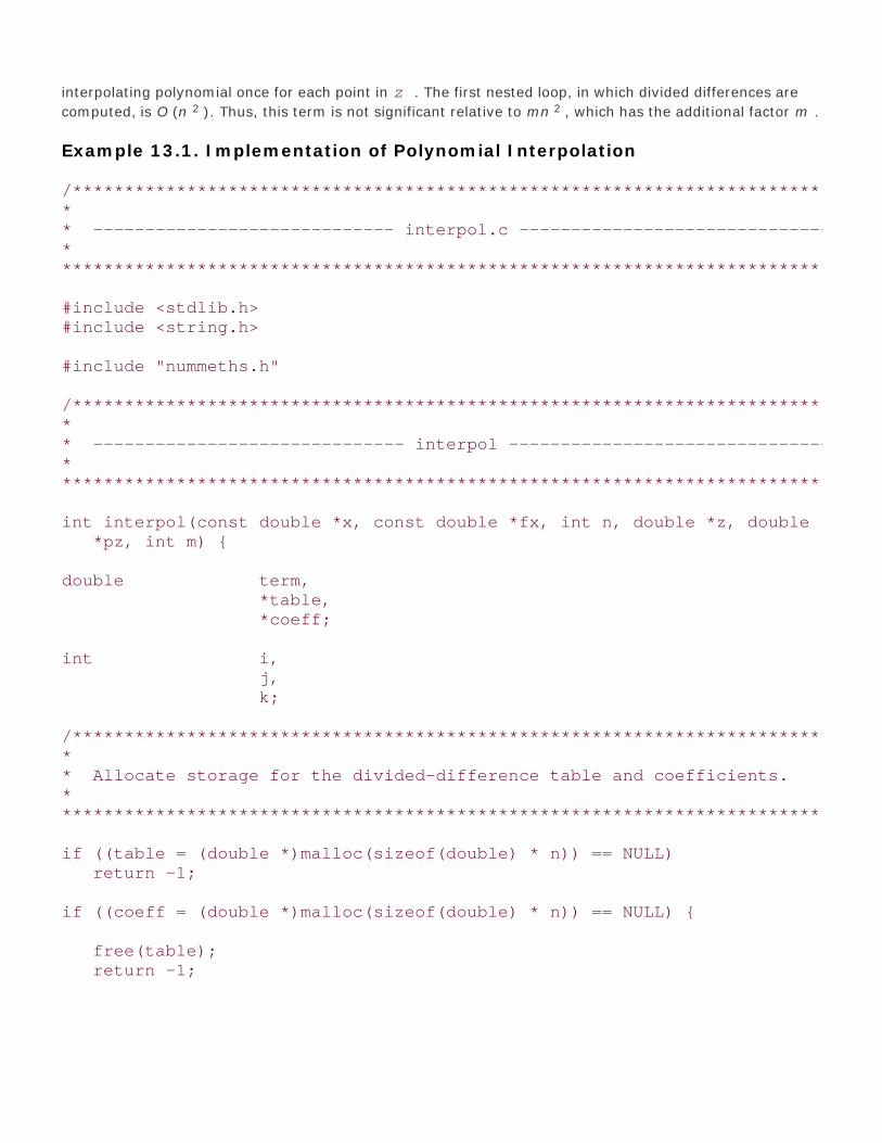
interpolating polynomial once for each point in z . The first nested loop, in which divided differences are
computed, is O (n 2 ). Thus, this term is not significant relative to mn 2 , which has the additional factor m .
Example 13.1. Implementation of Polynomial Interpolation
/****************************************************************************** ** ----------------------------- interpol.c ---------------------------------** ******************************************************************************/
#include <stdlib.h>#include <string.h>
#include "nummeths.h"
/****************************************************************************** ** ------------------------------ interpol -------------------------------- ** ******************************************************************************/
int interpol(const double *x, const double *fx, int n, double *z, double *pz, int m) {
double term, *table, *coeff;
int i, j, k;
/****************************************************************************** ** Allocate storage for the divided-difference table and coefficients. ** ******************************************************************************/
if ((table = (double *)malloc(sizeof(double) * n)) == NULL) return -1;
if ((coeff = (double *)malloc(sizeof(double) * n)) == NULL) {
free(table); return -1;

}
/****************************************************************************** ** Initialize the coefficients. ** ******************************************************************************/
memcpy(table, fx, sizeof(double) * n);
/****************************************************************************** ** Determine the coefficients of the interpolating polynomial. ** ******************************************************************************/
coeff[0] = table[0];
for (k = 1; k < n; k++) {
for (i = 0; i < n - k; i++) {
j = i + k; table[i] = (table[i + 1] - table[i]) / (x[j] - x[i]);
}
coeff[k] = table[0];
}
free(table);
/****************************************************************************** ** Evaluate the interpolating polynomial at the specified points. ** ******************************************************************************/
for (k = 0; k < m; k++) {
pz[k] = coeff[0];
for (j = 1; j < n; j++) {

term = coeff[j];
for (i = 0; i < j; i++) term = term * (z[k] - x[i]);
pz[k] = pz[k] + term;
}
}
free(coeff);
return 0;
}
Top

Mastering Algorithms with CBy Kyle Loudon
Slots : 1
Table of Contents
Chapter 13. Numerical Methods
Content
13.4 Description of Least-Squares Estimation
Least-squares estimation determines estimators b1 and b0 for a function y (x) = b1x + b0 so that y(x) is a best-fit line through a set of n points (x0, y0 ), . . ., (xn - 1, yn - 1). A best-fit line using least-squares estimation minimizes the sum of squared vertical distances between each point (xi, yi ), i =0, . . ., n - 1 and a corresponding point (xi, y (xi )) along y (x). This is one way of defining a line sothat each point (xi, yi ) is as close as possible to it.
Perhaps the most important application of least-squares estimation is to make inferences about alinear-form relationship between two variables. Given an independent variable x and a variable y thatdepends on it, estimators b1 and b0 allow us to calculate the expected value of y at values of x forwhich we have not actually observed y. This is particularly meaningful when x and y are related by astatistical relationship , which is an inexact relationship. For example, imagine how the number ofnew employees hired each month at a consulting firm is related to the number of hours the firm bills.Generally, as the firm hires more employees, it will bill more hours. However, there is not an exactnumber of hours it bills for a given number of employees. Contrast this with a functional relationship,which is exact. For example, a functional relationship might be one between the amount of moneythe firm charges for a project and the time the project requires. This relationship is exact if weassume that given a project of a certain length, there is an exact amount of money the firm willcharge.
To understand how least-squares estimation works, recall that the distance r between two points (x1,y1) and (x2, y2) is defined as:
Since the points (xi, yi ) and (xi, y (xi )) have the same x-coordinate, the line between them isvertical. Consequently, this formula tells us that the distance between these points is simply thedifference in y-coordinates, or |yi - y (xi )|. This difference is called the deviation of yi at xi.
Consider for a moment why the squared deviations are used to compute b1 and b0 , and not simplythe deviations themselves. The reason is primarily anachronistic. When we minimize the sum of theerrors, we end up with simultaneous equations that are linear. Before computers, these were theeasiest to solve. Another justification can be made on the basis of probability theory. Simply stated,the probability that b1 and b0 are optimal for the observed values of (xi, yi ) is proportional to anegative exponential containing the sum of all (yi - y (xi ))2. Thus, when we minimize the summationof squared deviations, we maximize the probability that b1 and b0 are good estimators as well. Yet

another justification is that by squaring the deviations, more emphasis is given to larger deviations.Since in a normal distribution there are fewer instances of large deviations, this gives more weight tothe deviations that occur less frequently.
To compute b1 and b0, we use the following formulas, where x and y are the coordinates of n points.These are derived from the simultaneous equations we mentioned above but did not show. The S(sigma) symbol in the formulas is used as a concise way of saying "sum all."
Figure 13.5 illustrates computing b1 and b0 for a set of n = 9 points (x0, y0 ), . . ., (x8, y8 ). Theresults of the calculations that need to be performed appear in the table. Using the values from thetable, b1 and b0 are calculated using:
Figure 13.5. Least-squares estimation and the best-fit line that results
Substituting these values into y (x) = b1x + b0 yields y (x) = 0.5519x - 0.0249. Figure 13.5 plots thisline with the points used to determine it. From the standpoint of least-squares estimation, no otherline is a better fit for the data than this one.
Top

Mastering Algorithms with CBy Kyle LoudonSlots : 1Table of ContentsChapter 13. Numerical Methods
Content
13.5 Interface for Least-Squares Estimationlsqe
void lsqe(const double *x, const double *y, int n, double *b1, double *b0);
Return Value
None.
Description
Uses least-squares estimation to obtain b 1 and b 0 in y (x ) = b 1 x + b 0 so that y (x ) is a best-fit line
through a set of points. The x -coordinates of the points are specified in x . The y -coordinates are
specified in y . The number of points is specified in n . The operation returns the appropriate values in b1and b0 .
Complexity
O (n ), where n is the number of points used in determining b 1 and b 0 .
Top

Mastering Algorithms with CBy Kyle LoudonSlots : 1Table of ContentsChapter 13. Numerical Methods
Content
13.6 Implementation and Analysis of Least-SquaresEstimation
The implementation of least-squares estimation presented here requires us to do little more than computea few summations and apply the results to the formulas presented earlier. The operation begins by
summing all values for xi in sumx , all values for yi in sumy , all values of xi 2 in sumx2 , and all values
of xi yi in sumxy (see Example 13-2 ). Once we have completed this, we compute b 1 and b 0 using the
formulas presented earlier.
The runtime complexity of lsqe is O (n ), where n is the number of points used to determine b 1 and b 0 .This is because a single loop that iterates n times is used to compute the summations.
Example 13.2. Implementation of Least-Squares Estimation
/****************************************************************************** ** -------------------------------- lsqe.c -------------------------------- ** ******************************************************************************/
#include <math.h>
#include "nummeths.h"
/****************************************************************************** ** --------------------------------- lsqe --------------------------------- ** ******************************************************************************/
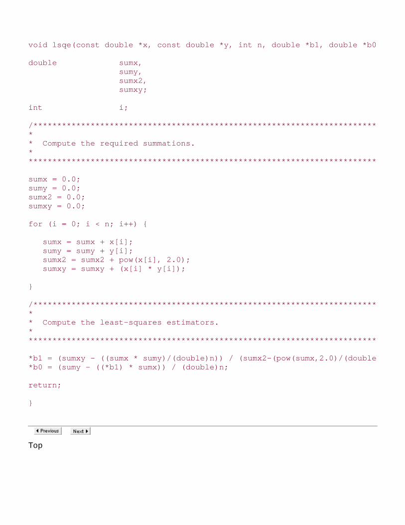
void lsqe(const double *x, const double *y, int n, double *b1, double *b0) {
double sumx, sumy, sumx2, sumxy;
int i;
/****************************************************************************** ** Compute the required summations. ** ******************************************************************************/
sumx = 0.0;sumy = 0.0;sumx2 = 0.0;sumxy = 0.0;
for (i = 0; i < n; i++) {
sumx = sumx + x[i]; sumy = sumy + y[i]; sumx2 = sumx2 + pow(x[i], 2.0); sumxy = sumxy + (x[i] * y[i]);
}
/****************************************************************************** ** Compute the least-squares estimators. ** ******************************************************************************/
*b1 = (sumxy - ((sumx * sumy)/(double)n)) / (sumx2-(pow(sumx,2.0)/(double)n));*b0 = (sumy - ((*b1) * sumx)) / (double)n;
return;
}
Top

Mastering Algorithms with CBy Kyle Loudon
Slots : 1
Table of Contents
Chapter 13. Numerical Methods
Content
13.7 Description of the Solution of Equations
One of the most fundamental problems in scientific computing is solving equations of the form f (x) =0. This is often referred to as finding the roots, or zeros, of f (x). Here, we are interested in the realroots of f (x), as opposed to any complex roots it might have. Specifically, we will focus on findingreal roots when f (x) is a polynomial.
13.7.1 Finding Roots with Newton's Method
Although factoring and applying formulas are simple ways to determine the roots of polynomialequations, a great majority of the time polynomials are of a large enough degree and sufficientlycomplicated that we must turn to some method of approximation. One of the best approaches isNewton's method. Fundamentally, Newton's method looks for a root of f (x) by moving closer andcloser to it through a series of iterations. We begin by choosing an initial value x = x0 that we think isnear the root we are interested in. Then, we iterate using the formula:
until xi + 1 is a satisfactory approximation. In this formula, f (x) is the polynomial for which we aretrying to find a root, and f ' (x) is the derivative of f (x).
13.7.2 Computing the Derivative of a Polynomial
The derivative of a function is fundamental to calculus and can be described in many ways. For now,let's simply look at a formulaic description, specifically for polynomials. To compute the derivative ofa polynomial, we apply to each of its terms one of two formulas:
where k is a constant, r is a rational number, and x is an unknown. The symbol d /dx means"derivative of," where x is the variable in the polynomial. For each term that is a constant, we applythe first formula; otherwise, we apply the second. For example, suppose we have the function:

In order to compute f ' (x), the derivative of f (x), we apply the second formula to the first threeterms of the polynomial, and the first formula to the last term, as follows:
Sometimes it is necessary to compute higher-order derivatives as well, which are derivatives ofderivatives. For example, the second derivative of f (x), written f '' (x), is the derivative of f ' (x).Similarly, the third derivative of f (x), written f ''' (x), is the derivative of f '' (x), and so forth. Thus,to compute the second derivative of f (x) in the previous equation, we compute the derivative of f '(x), as follows:
13.7.3 Understanding the First and Second Derivative
Now let's look at what derivatives really mean. To use Newton's method properly, it is important tounderstand the meaning of the first and second derivative in particular.
The value of the first derivative of f (x) at some point x = x0 indicates the slope of f (x) at point x0;that is, whether f (x) is increasing (sloping upward from left to right) or decreasing (slopingdownward). If the value of the derivative is positive, f (x) is increasing; if the value is negative, f (x)is decreasing; if the value is zero, f (x) is neither increasing nor decreasing. The magnitude of thevalue indicates how fast f (x) is increasing or decreasing. For example, Figure 13.6, example a,depicts a function whose value increases within the shaded regions; thus, these are the regionswhere the first derivative is positive. The plot of the first derivative crosses the x-axis at the pointswhere the slope of f (x) changes sign.
The value of the second derivative of f (x) at some point x = x0 indicates the concavity of f (x) atpoint x0, that is, whether the function is opening upward or downward. The magnitude of the valueindicates how extreme the concavity is. In Figures 13-6a and 13-6c, the dotted line indicates thepoint at which the concavity of the function changes sign. This is the point at which the plot of thesecond derivative crosses the x-axis.
Another way to think of the value of the derivative of f (x) at some point x = c is as the slope of theline tangent to f (x) at c, expressed in point-slope form. The point-slope form of a line is:
Thus, if f (x) = x 3 - x 2 - 3x + 1.8 as shown in Figure 13.6, example a, the equation of the linetangent to f (x) at c = 1.5 as can be determined as follows. Figure 13.6, example d, is a plot of thisline along with f (x).

Figure 13.6. The meaning of the first and second derivatives of f (x)
13.7.4 Selecting an Initial Point for Newton's Method
Now that we understand a little about derivatives, let's return to Newton's method. Paramount toNewton's method is the proper selection of an initial iteration point x0. In order for Newton's methodto converge to the root we are looking for, the initial iteration point must be "near enough" and onthe correct side of the root we are seeking. There are two rules that must be followed to achieve this:
Determine an interval [a, b ] for x0 where one and only one root exists. To do this, choose aand b so that the signs of f (a) and f (b) are not the same and f ' (x) does not change sign. If f(a) and f (b) have different signs, the interval contains at least one root. If the sign of f ' (x)does not change on [a, b ], the interval contains only one root because the function can onlyincrease or decrease on the interval.
1.
Choose either x0 = a or x0 = b so that f (x0) has the same sign as f '' (x) on the interval [a, b ].This also implies that f '' (x) does not change sign on the interval. Recall that the secondderivative of f (x) is an indication of concavity. If f '' (x) does not change sign and x0 is chosenso that f (x0) has the same sign as f '' (x), each successive iteration of Newton's method willconverge closer to the root on the interval [a, b ] (see Figure 13.7).
2.
In each of the four parts of Figure 13.7, f (x) is shown as a heavy line, and a and b are shown asvertical dotted lines. If f (a) matches the criteria just given, iteration begins at a and tangent linesslope from a toward the root to which we would like to converge. If f (b) matches the criteria above,iteration begins at b and tangent lines slope from b toward the root to which we would like to

converge.
Figure 13.7. Convergence of Newton's method
13.7.5 How Newton's Method Works
As an example, suppose we would like to find the roots of f (x) = x 3 - x2 - 3x + 1.8. Figure 13-8illustrates that this function appears to have three roots: one on the interval [-2, -1], another on theinterval [0, -1], and a third on the interval [2, 3]. Once we have an idea of the number and locationof a function's roots, we test each interval against the rules for selecting an initial iteration point. Todo this, we need to know the following:
Using this information, we see that the interval [-2, -1] satisfies the first rule because f (-2) = -4.2and f (-1) = 2.8, and f ' (x) does not change sign on the interval: it is always positive. Consideringthis, we know there is, in fact, one and only one root on the interval [-2, -1]. To satisfy the secondrule, we see that f '' (x) does not change sign on the interval: it is negative. We select x0 = -2 as theinitial iteration point since f (-2) = -4.2 is also negative. Figure 13.8 illustrates calculating the root onthis interval to within 0.0001 of its actual value. We end up iterating five times to obtain thisapproximation.
Figure 13.8. Calculating the three real roots of f (x) = x3 - x2 - 3x + 1.8 =0 to within 0.0001 of their actual values

Moving to the root on the interval [0, 1], we see that the first rule is satisfied just as for the previousinterval. However, the sign of f '' (x) is not constant on this interval; therefore, the interval does notsatisfy the second rule. Suspecting that the root is closer to 1 than 0, we try the interval [0.5, 1]next, which corrects the problem. The first rule is satisfied because f (0.5) = 0.175 and f (1) = -1.2,and f ' (x) does not change sign on the interval: it is negative. To complete the second rule, we selectx0 = 0.5 since f (0.5) = 0.175 is positive and has the same sign as f '' (x) over the interval [0.5, 1].Figure 13.8 illustrates calculating the root on this interval to within 0.0001 of its actual value. We endup iterating four times to obtain this approximation. Calculating the third root proceeds in a similarmanner.
Top

Mastering Algorithms with CBy Kyle LoudonSlots : 1Table of ContentsChapter 13. Numerical Methods
Content
13.8 Interface for the Solution of Equationsroot
int root(double (*f)(double x), double (*g)(double x), double *x, int *n, double delta)
Return Value
0if a root is found, -1 otherwise.
Description
Computes the root of f to which Newton's method converges given an initial iteration point. This point is
specified in x[0] . The derivative of f is specified in g . The argument n is the maximum number of
iterations to perform. The argument delta is the difference between successive approximations at which
to stop iterating. Upon return, successive values of x calculated during the iteration process are returned
in the x array. Upon return, n contains the number of values in array x . It is the responsibility of the
caller to manage the storage associated with x .
Complexity
O (n ), where n is the maximum number of iterations the caller wishes to perform.
Top

Mastering Algorithms with CBy Kyle LoudonSlots : 1Table of ContentsChapter 13. Numerical Methods
Content
13.9 Implementation and Analysis of the Solution ofEquations
Recall that solving an equation of the form f (x ) = means finding its roots. The root operation locates thereal root to which Newton's method converges given an initial iteration point.
The root operation revolves around a single loop (see Example 13-3 ), which calculates successive
approximations using the Newton iteration formula. In the implementation presented here, f is the
function for which we are approximating the root, and g is the derivative of f . After each iteration, we
determine whether the current approximation of the root is satisfactory. An approximation is deemed
satisfactory when the difference between it and that of the previous iteration is less than delta . If after
n iterations a satisfactory root still has not been found, root terminates.
The runtime complexity of root is O (n ), where n is the maximum number of iterations the caller wishes toperform. The worst case occurs when we do not find the root we are looking for.
Example 13.3. Implementation for the Solution of Equations
/****************************************************************************** ** -------------------------------- root.c -------------------------------- ** ******************************************************************************/
#include <math.h>
#include "nummeths.h"
/*****************************************************************************

* ** --------------------------------- root --------------------------------- ** ******************************************************************************/
int root(double (*f)(double x), double (*g)(double x), double *x, int *n, double delta) {
int satisfied, i;
/****************************************************************************** ** Use Newton's method to find a root of f. ** ******************************************************************************/
i = 0;satisfied = 0;
while (!satisfied && i + 1 < *n) {
/************************************************************************** * * * Determine the next iteration of x. * * * **************************************************************************/
x[i + 1] = x[i] - (f(x[i]) / g(x[i]));
/************************************************************************** * * * Determine whether the desired approximation has been obtained. * * * **************************************************************************/
if (fabs(x[i + 1] - x[i]) < delta) satisfied = 1;
/************************************************************************** * * * Prepare for the next iteration. * * * **************************************************************************/
i++;

}
/****************************************************************************** ** Even without iterating, indicate that one value has been stored in x. ** ******************************************************************************/
if (i == 0) *n = 1;else *n = i + 1;
/****************************************************************************** ** Return whether a root was found or the maximum iterations were reached. ** ******************************************************************************/
if (satisfied) return 0;else return -1;
}
Top

Mastering Algorithms with CBy Kyle Loudon
Slots : 1
Table of Contents
Chapter 13. Numerical Methods
Content
13.10 Questions and Answers
Q: In the discussion of polynomial interpolation, we stated that we need to choose enough points togive an accurate impression of the function we are interpolating. What happens if we do not useenough points?
A: Interpolating a function with not enough points, or poorly placed points, leads to an interpolatingpolynomial that does not accurately reflect the function we think we are interpolating. A simpleexample is interpolating a quadratic polynomial (a parabola when plotted) with only two points.Interpolation with two points results in a line, which is far from a parabola!
Q: Using the guidelines presented in this chapter, how many interpolation points should we use tointerpolate the function f (x) = x 5 + 2.8x 3 - 3.3x 2 - x + 4.1?
A: When interpolating a function that we know is a polynomial itself, we can get a good impression ofthe function by using n + 1 well-placed points, where n is the degree of the polynomial. In thisexample, the polynomial has a degree of 5, so we should use six well-placed interpolation points. Thisresults in an interpolating polynomial that has the same degree as f (x).
Q: Recall that to approximate a root of an equation using Newton's method, we select an interval [a,b] on which the root exists and iterate closer and closer to it. What if we choose this interval muchlarger than needed, but in such a way that both rules mentioned in this chapter are still satisfied?
A: The discussion of Newton's method mentioned two rules that must be satisfied in order toguarantee the algorithm's success: we need to determine an interval [a, b ] where one and only oneroot exists; and we need to choose x0, the initial iteration point, so that f (x0) has the same sign as f'' (x) over the interval. Provided these rules are satisfied, the interval [a, b ] can be as large as wewould like to make it. However, Newton's method will require more iterations to converge if we usean interval that is excessively large. Therefore, typically a relatively small interval convenient to theproblem should be chosen.
Q: In the implementation of root, what symptoms might we notice if we have violated one the rulesof Newton's method that guarantee convergence?
A: If we follow the rules presented in this chapter, Newton's method guarantees convergence to theroot that exists on the interval [a, b ] containing the initial iteration point, x0. Various symptoms helpto determine when we have violated these rules. For example, successive approximations thatappear to be diverging instead of converging indicate a problem. Another symptom is convergence to

a root other than the one we expect. For example, suppose we think there is a root near -2 (perhapsby plotting the function), but we end up finding a root near 9. In order to relay these symptoms backto the caller, root returns both an array of the approximations obtained in successive iterations ofNewton's method and an array of values for f (x) computed using the approximations. Normally,successive values for f (x) should approach 0. The parameter n of the root operation provides a wayto keep a divergent series from running too long.
Top

Mastering Algorithms with CBy Kyle Loudon
Slots : 1
Table of Contents
Chapter 13. Numerical Methods
Content
13.11 Related Topics
Error approximation
An important part of more substantial work with numerical methods. Numerical analysis isreplete with approximation methods, and inherent in any approximation is some amount oferror. Often it is important to quantify this.
Derivatives of functions
A fundamental part of calculus. The numerical methods presented in this chapter required onlya primitive understanding of derivatives. However, for many numerical methods, a morecomplete understanding of derivatives and calculus is essential.
Muller's method
An algorithm for finding both the real and complex roots of equations. Complex roots arecomplex numbers, which result from taking the square root of negative numbers. This chapterfocused on finding real roots.
Top

Mastering Algorithms with CBy Kyle LoudonSlots : 1Table of ContentsPart III: Algorithms
Content
Chapter 14. Data CompressionData compression is the process of reducing the number of bits used to represent data. It is one of themost significant results of information theory , an area of mathematics that addresses various ways tomanage and manipulate information. Data compression entails two processes: in one process the data iscompressed, or encoded , to reduce its size; in a second process it is uncompressed, or decoded , to returnit to its original state.
To understand why data compression is possible, we must first understand that all data can becharacterized by some informational content, called its entropy (a term borrowed from thermodynamics) .Compression is possible because most data is represented with more bits than its entropy suggests isoptimal. To gauge the effectiveness of compression, we look at the ratio of the size of the compressed datadivided by its original size, and subtract this from 1. This value is known as the data's compression ratio .
In the broadest sense, data compression methods are divided into two classes: lossy and lossless . In lossycompression we accept a certain loss of accuracy in exchange for greater compression ratios. This isacceptable in some applications, such as graphics and sound processing, provided the degradation ismanaged carefully. However, frequently we use lossless compression, which ensures that an exact copy ofthe original data is reproduced when uncompressed.
This chapter focuses on lossless compression, for which there are two general approaches: minimumredundancy coding and dictionary-based methods . Minimum redundancy coding achieves compression byencoding symbols that occur with great frequency using fewer bits than for those that occur less often.Dictionary-based methods encode data in terms of tokens that take the place of redundant phrases.Example 14.1 is a header for the compression methods presented in this chapter.
This chapter covers:
Bit operations
An important part of data compression because most methods require operating on data one bit at atime to some degree. C provides a number of bitwise operators that can be used to implement anextended class of bit operations.

Huffman coding
One of the oldest and most elegant forms of compression based on minimum redundancy coding.Fundamental to Huffman coding is the construction of a Huffman tree, which is used both to encodeand decode the data. Huffman coding is not the most effective form of compression, but it runs fastboth when compressing and uncompressing data.
LZ77 (Lempel-Ziv-1977)
One of the fundamental methods of dictionary-based compression. LZ77 uses a sliding window and alook-ahead buffer to encode symbols in terms of phrases encountered earlier in the data. LZ77generally results in better compression ratios than Huffman coding, but with longer compressiontimes. However, uncompressing data is generally very fast.
Some applications of lossless data compression are :
Software distribution
The process of delivering software on various media. When distributing software on physical media,such as compact discs or magnetic tapes and diskettes, reducing the amount of storage required canproduce considerable cost savings in mass distributions.
Archiving
Collecting groups of files into organized libraries. Typically, archives contain large amounts of data.Thus, after creating archives, frequently we compress them.
Mobile computing
An area of computing in which devices typically have limited amounts of memory and secondarystorage. Mobile computing generally refers to computing with small, portable devices such asadvanced programmable calculators, electronic organizers, and other personal computing devices.
Optimized networking (illustrated in this chapter)
Compression is used especially when sending large amounts of data across wide-area networks.Bandwidth at certain points along wide-area networks is often limited. Although compressing anduncompressing data does require time, in many network applications the cost is well justified.
Embedded applications
An area of computing similar to mobile computing in that devices typically have somewhat limitedamounts of memory and secondary storage. Examples of embedded applications are lab instruments,avionics (aircraft electronics), VCRs, home stereos, and other pieces of equipment built aroundmicrocontrollers.
Database systems
Typically, large systems that can be optimized by reducing their size to some extent. Databases maybe compressed at the record or file level.
Online manuals
Manuals that are accessed directly on a computer. Online manuals are typically of considerable size,but many sections are not accessed on a regular basis. Therefore, it is common to store them in acompressed form and uncompress sections only as they are needed.
Example 14.1. Header for Data Compression
/*****************************************************************************

* ** ------------------------------ compress.h ------------------------------ ** ******************************************************************************/
#ifndef COMPRESS_H#define COMPRESS_H
#include "bitree.h"
/****************************************************************************** ** Define a structure for nodes of Huffman trees. ** ******************************************************************************/
typedef struct HuffNode_ {
unsigned char symbol;int freq;
} HuffNode;
/****************************************************************************** ** Define a structure for entries in Huffman code tables. ** ******************************************************************************/
typedef struct HuffCode_ {
unsigned char used;unsigned short code;unsigned char size;
} HuffCode;
/****************************************************************************** ** Define the number of bits required for LZ77 token members. ** ******************************************************************************/
#define LZ77_TYPE_BITS 1#define LZ77_WINOFF_BITS 12#define LZ77_BUFLEN_BITS 5
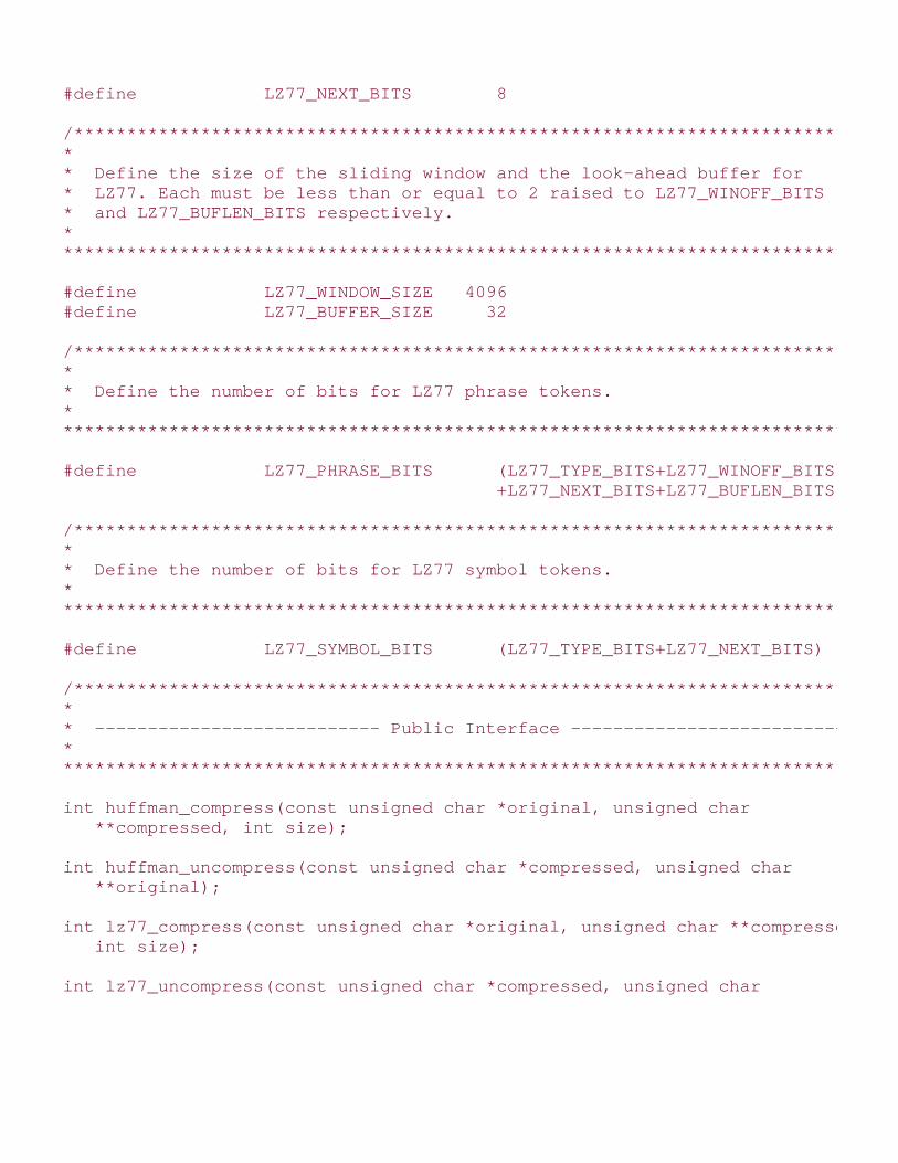
#define LZ77_NEXT_BITS 8
/****************************************************************************** ** Define the size of the sliding window and the look-ahead buffer for ** LZ77. Each must be less than or equal to 2 raised to LZ77_WINOFF_BITS ** and LZ77_BUFLEN_BITS respectively. ** ******************************************************************************/
#define LZ77_WINDOW_SIZE 4096#define LZ77_BUFFER_SIZE 32
/****************************************************************************** ** Define the number of bits for LZ77 phrase tokens. ** ******************************************************************************/
#define LZ77_PHRASE_BITS (LZ77_TYPE_BITS+LZ77_WINOFF_BITS\ +LZ77_NEXT_BITS+LZ77_BUFLEN_BITS)
/****************************************************************************** ** Define the number of bits for LZ77 symbol tokens. ** ******************************************************************************/
#define LZ77_SYMBOL_BITS (LZ77_TYPE_BITS+LZ77_NEXT_BITS)
/****************************************************************************** ** --------------------------- Public Interface --------------------------- ** ******************************************************************************/
int huffman_compress(const unsigned char *original, unsigned char **compressed, int size);
int huffman_uncompress(const unsigned char *compressed, unsigned char **original);
int lz77_compress(const unsigned char *original, unsigned char **compressed, int size);
int lz77_uncompress(const unsigned char *compressed, unsigned char

**original);
#endif
Top

Mastering Algorithms with CBy Kyle Loudon
Slots : 1
Table of Contents
Chapter 14. Data Compression
Content
14.1 Description of Bit Operations
When compressing and uncompressing data, often we need to perform operations on less than asingle byte. Therefore, before discussing various methods of data compression, it is important tobecome familiar with some basic operations for working with data one bit at a time. These operationsare necessary because bit operators in C work only with intrinsic integral operands, which are small.The operations presented in this section work with buffers containing any number of bits. Note thatthe set of operations presented here is rather incomplete. Specifically, only those that are used inthis chapter and in Chapter 15, are defined.
Top

Mastering Algorithms with CBy Kyle Loudon
Slots : 1
Table of Contents
Chapter 14. Data Compression
Content
14.2 Interface for Bit Operations
bit_ get
int bit_get(const unsigned char *bits, int pos);
Return Value
State of the desired bit: 1 or 0.
Description
Gets the state of the bit at position pos in the buffer bits. The leftmost position in the buffer is 0.The state returned is either 1 or 0.
Complexity
O (1)
bit_set
void bit_set(unsigned char *bits, int pos, int state);
Return Value
None.
Description

Sets the state of the bit at position pos in the buffer bits to the value specified by state. Theleftmost position in the buffer is 0. The state must be 1 or 0.
Complexity
O (1)
bit_xor
void bit_xor(const unsigned char *bits1, const unsigned char *bits2, unsigned char *bitsx, int size);
Return Value
None.
Description
Computes the bitwise XOR (exclusive OR) of the two buffers bits1 and bits2, each containingsize bits, and returns the result in bitsx. The bitwise XOR of two binary operands yields in eachposition i of the result where in position i of the operands the bits are the same, and 1 in each position
where the bits are different. For example, 11010 01011 = 10001 ( denotes XOR). It is theresponsibility of the caller to manage the storage required by bitsx.
Complexity
O (b), where b is the number of bits in each buffer.
bit_rot_left
void bit_rot_left(unsigned char *bits, int size, int count);
Return Value
None.
Description
Rotates the buffer bits, containing size bits, to the left count bits. After the operation, theleftmost count bits become the count rightmost bits in the buffer, and all other bits are shiftedaccordingly.

Complexity
O (n b), where n is the number of bits rotated to the left and b is the number of bits in the buffer.
Top

Mastering Algorithms with CBy Kyle LoudonSlots : 1Table of ContentsChapter 14. Data Compression
Content
14.3 Implementation and Analysis of Bit Operations
Each bit operation works with a buffer of data defined as a pointer to an unsigned character. This pointerpoints to as many bytes as are required to represent the number of bits in the buffer. If the number of bitsin the buffer is not a multiple of 8, some bits in the final byte are not used.
14.3.1 bit_ get
The bit_ get operation gets the state of a bit in a buffer (see Example 14.2 ). To do this, we determine inwhich byte the desired bit resides and then use a mask to get the specific bit from that byte. The bit set to
1 in mask determines which bit will be read from the byte. We use a loop to shift this bit into the proper
position. We fetch the desired bit by indexing to the appropriate byte in bits and applying the mask.
The runtime complexity of bit_ get is O (1). This is because all of the steps in getting the state of a bit in abuffer run in a constant amount of time.
14.3.2 bit_set
The bit_set operation sets the state of a bit in a buffer (see Example 14.2 ). This operation works similarlyto bit_ get , except that it uses the mask to set the state of the specified bit rather than to get it.
The runtime complexity of bit_set is O (1). This is because all of the steps in getting the state of a bit in abuffer run in a constant amount of time.
14.3.3 bit_xor
The bit_xor operation computes the bitwise XOR (exclusive OR) of two buffers, bits1 and bits2 , and
places the result in another buffer, bitsx (see Example 14.2 ). To do this, we compare the bit in position
i of bits1 with the bit in position i of bits2 . If the bits are the same, we set the bit in position iof bitsx to 0; otherwise, we set the bit in position i of bitsx to 1. This process continues for as

many bits are in each buffer, as specified by size .
The runtime complexity of bit_xor is O (b ), where b is the number of bits in each buffer. This is becausethe loop in the operation iterates once for each bit.
14.3.4 bit_rot_left
The bit_rot_left operation rotates a buffer a specified number of bits to the left (see Example 14.2 ). Webegin by saving the leftmost bit of the leftmost byte and then shifting each byte one bit to the left. As weshift each byte, we set the rightmost bit of the preceding byte to the bit shifted off the left of the currentbyte. Once we have shifted the last byte, we set its rightmost bit to the bit shifted off the first byte. Thisprocess is repeated as many times as the number of bits to be rotated.
The runtime complexity of bit_rot_left is O (n b ), where n is the number of bits rotated to the left and b isthe number of bits in the buffer. This is because for each rotation, (b /8) + 1 shifts are performed to theleft.
Example 14.2. Implementation of Bit Operations
/****************************************************************************** ** --------------------------------- bit.c -------------------------------- ** ******************************************************************************/
#include <string.h>
#include "bit.h"
/****************************************************************************** ** -------------------------------- bit_get ------------------------------- ** ******************************************************************************/
int bit_get(const unsigned char *bits, int pos) {
unsigned char mask;
int i;
/****************************************************************************** ** Set a mask for the bit to get. ** ******************************************************************************/

mask = 0x80;
for (i = 0; i < (pos % 8); i++) mask = mask >> 1;
/****************************************************************************** ** Get the bit. ** ******************************************************************************/
return (((mask & bits[(int)(pos / 8)]) == mask) ? 1 : 0);
}
/****************************************************************************** ** -------------------------------- bit_set ------------------------------- ** ******************************************************************************/
void bit_set(unsigned char *bits, int pos, int state) {
unsigned char mask;
int i;
/****************************************************************************** ** Set a mask for the bit to set. ** ******************************************************************************/
mask = 0x80;
for (i = 0; i < (pos % 8); i++) mask = mask >> 1;
/****************************************************************************** ** Set the bit. ** ******************************************************************************/
if (state) bits[pos / 8] = bits[pos / 8] | mask;

else bits[pos / 8] = bits[pos / 8] & (~mask);
return;
}
/****************************************************************************** ** -------------------------------- bit_xor ------------------------------- ** ******************************************************************************/
void bit_xor(const unsigned char *bits1, const unsigned char *bits2, unsigned char *bitsx, int size) {
int i;
/****************************************************************************** ** Compute the bitwise XOR (exclusive OR) of the two buffers. ** ******************************************************************************/
for (i = 0; i < size; i++) {
if (bit_ get(bits1, i) != bit_ get(bits2, i)) bit_set(bitsx, i, 1); else bit_set(bitsx, i, 0);
}
return;
}
/****************************************************************************** ** ----------------------------- bit_rot_left ----------------------------- ** ******************************************************************************/
void bit_rot_left(unsigned char *bits, int size, int count) {
int fbit,

lbit, i, j;
/****************************************************************************** ** Rotate the buffer to the left the specified number of bits. ** ******************************************************************************/
if (size > 0) {
for (j = 0; j < count; j++) {
for (i = 0; i <= ((size - 1) / 8); i++) {
/******************************************************************** * * * Get the bit about to be shifted off the current byte. * * * ********************************************************************/
lbit = bit_get(&bits[i], 0);
if (i == 0) {
/***************************************************************** * * * Save the bit shifted off the first byte for later. * * * *****************************************************************/
fbit = lbit;
}
else {
/***************************************************************** * * * Set the rightmost bit of the previous byte to the leftmost * * bit about to be shifted off the current byte. * * * *****************************************************************/
bit_set(&bits[i - 1], 7, lbit);
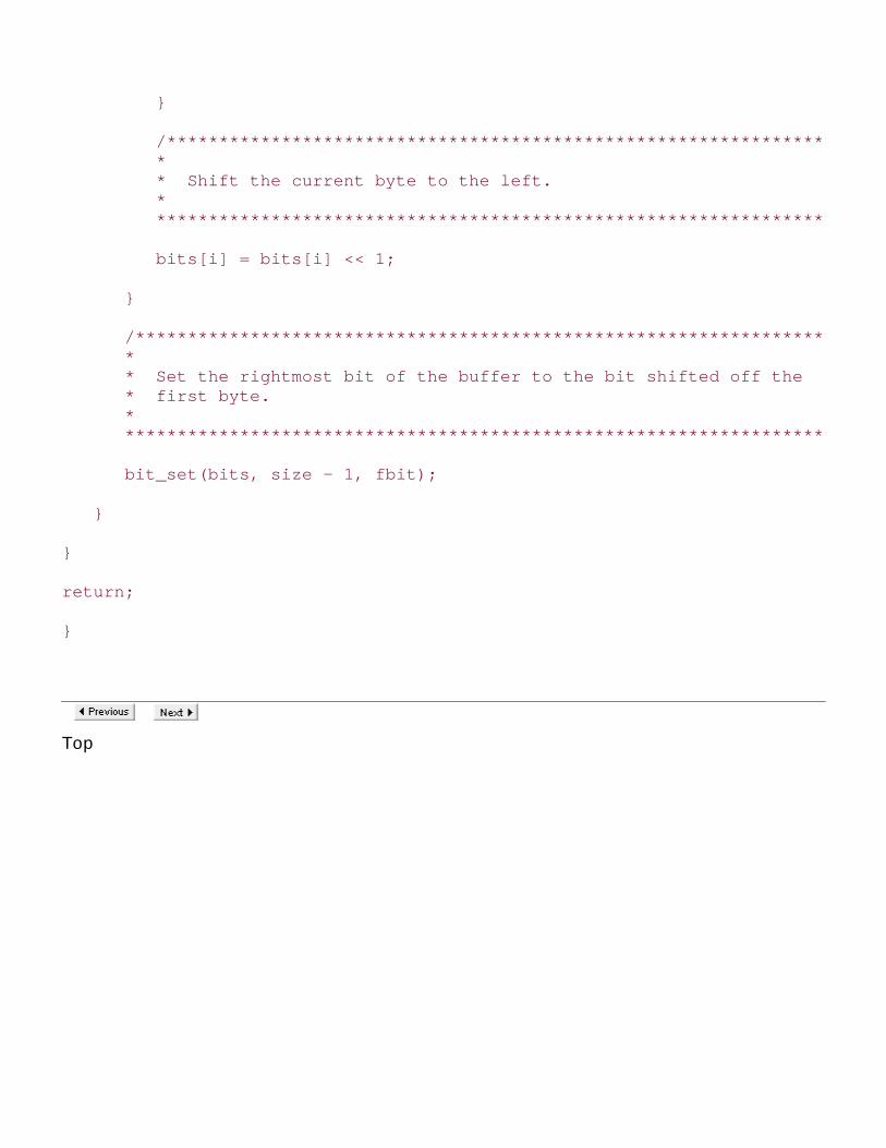
}
/******************************************************************** * * * Shift the current byte to the left. * * * ********************************************************************/
bits[i] = bits[i] << 1;
}
/*********************************************************************** * * * Set the rightmost bit of the buffer to the bit shifted off the * * first byte. * * * ***********************************************************************/
bit_set(bits, size - 1, fbit);
}
}
return;
}
Top

Mastering Algorithms with CBy Kyle Loudon
Slots : 1
Table of Contents
Chapter 14. Data Compression
Content
14.4 Description of Huffman Coding
One of the oldest and most elegant forms of data compression is Huffman coding, an algorithm basedon minimum redundancy coding. Minimum redundancy coding suggests that if we know how oftendifferent symbols occur in a set of data, we can represent the symbols in a way that makes the datarequire less space. The idea is to encode symbols that occur more frequently with fewer bits thanthose that occur less frequently. It is important to realize that a symbol is not necessarily a characterof text: a symbol can be any amount of data we choose, but it is often one byte's worth.
14.4.1 Entropy and Minimum Redundancy
To begin, let's revisit the concept of entropy introduced at the beginning of the chapter. Recall thatevery set of data has some informational content, which is called its entropy. The entropy of a set ofdata is the sum of the entropies of each of its symbols. The entropy S of a symbol z is defined as:
Sz = -lgPz
where Pz is the probability of z being found in the data. If it is known exactly how many times zoccurs, Pz is referred to as the frequency of z. As an example, if z occurs 8 times in 32 symbols, orone-fourth of the time, the entropy of z is:
-lg(1/4) = 2 bits
This means that using any more than two bits to represent z is more than we need. If we considerthat normally we represent a symbol using eight bits (one byte), we see that compression here hasthe potential to improve the representation a great deal.
Table 14.1 presents an example of calculating the entropy of some data containing 72 instances offive different symbols. To do this, we sum the entropies contributed by each symbol. Using "U" as anexample, the total entropy for a symbol is computed as follows. Since "U" occurs 12 times out of the72 total, each instance of "U" has an entropy that is calculated as:
-lg(12/72) = 2.584963 bits
Consequently, because "U" occurs 12 times in the data, its contribution to the entropy of the data iscalculated as:

(2.584963)(12) = 31.01955 bits
In order to calculate the overall entropy of the data, we sum the total entropies contributed by eachsymbol. To do this for the data in Table 14.1, we have:
31.01955+36.000000+23.53799+33.94552+36.95994 = 161.46300 bits
If using 8 bits to represent each symbol yields a data size of (72)(8) = 576 bits, we should be able tocompress this data, in theory, by up to:
1-(161.463000/576) = 72.0%
Table 14.1. The Entropy of a Set of Data Containing 72 Instances of 5Different Symbols
Symbol Probability Entropy of Each Instance Total Entropy
U 12/72 2.584963 31.01955
V 18/72 2.000000 36.00000
W 7/72 3.362570 23.53799
X 15/72 2.263034 33.94552
Y 20/72 1.847997 36.95994
14.4.2 Building a Huffman Tree
Huffman coding presents a way to approximate the optimal representation of data based on itsentropy. It works by building a data structure called a Huffman tree, which is a binary tree (seeChapter 9) organized to generate Huffman codes. Huffman codes are the codes assigned to symbolsin the data to achieve compression. However, Huffman codes result in compression that onlyapproximates the data's entropy because, as you may have noticed in Table 14.1, the entropies ofsymbols often come out to be fractions of bits. Since the actual number of bits used in Huffmancodes cannot be fractions in practice, some codes end up with slightly too many bits to be optimal.
Figure 14.1 illustrates the process of building a Huffman tree from the data in Table 14.1. Building aHuffman tree proceeds from its leaf nodes upward. To begin, we place each symbol and its frequencyin its own tree (see Figure 14.1, step 1). Next, we merge the two trees whose root nodes have thesmallest frequencies and store the sum of the frequencies in the new tree's root (see Figure 14.1,step 2). This process is then repeated until we end up with a single tree (see Figure 14.1, step 5),which is the final Huffman tree. The root node of this tree contains the total number of symbols in thedata, and its leaf nodes contain the original symbols and their frequencies. Because Huffman codingcontinually seeks out the two trees that appear to be the best to merge at any given time, it is agood example of a greedy algorithm (see Chapter 1).
Figure 14.1. Building a Huffman tree from the symbols and frequencies inTable 14.1

14.4.3 Compressing and Uncompressing Data
Building a Huffman tree is part of both compressing and uncompressing data. To compress datausing a Huffman tree, given a specific symbol, we start at the root of the tree and trace a path to thesymbol's leaf. As we descend along the path, whenever we move to the left, we append to thecurrent code; whenever we move to the right, we append 1. Thus, in Figure 14.1, step 6, todetermine the Huffman code for "U" we move to the right (1), then to the left (10), and then to theright again (101). The Huffman codes for all of the symbols in the figure are:
U = 101, V = 01, W = 100, X = 00, Y = 11
To uncompress data using a Huffman tree, we read the compressed data bit by bit. Starting at thetree's root, whenever we encounter in the data, we move to the left in the tree; whenever weencounter 1, we move to the right. Once we reach a leaf node, we generate the symbol it contains,move back to the root of the tree, and repeat the process until we exhaust the compressed data.Uncompressing data in this manner is possible because Huffman codes are prefix free, which meansthat no code is a prefix of any other. This ensures that once we encounter a sequence of bits thatmatches a code, there is no ambiguity as to the symbol it represents. For example, notice that 01,the code for "V," is not a prefix of any of the other codes. Thus, as soon as we encounter 01 in thecompressed data, we know that the code must represent "V."

14.4.4 Effectiveness of Huffman Coding
To determine the reduced size of data compressed using Huffman coding, we calculate the product ofeach symbol's frequency times the number of bits in its Huffman code, then add them together.Thus, to calculate the compressed size of the data presented in Table 14.1 and Figure 14.1, we have:
(12)(3)+(18)(2)+(7)(3)+(15)(2)+(20)(2) = 163 bits
Assuming that without compression each of the 72 symbols would be represented with 8 bits, for atotal data size of 576 bits, we end up with the following compression ratio:
1-(163/576)=71.7%
Once again, considering the fact that we cannot take into account fractional bits in Huffman coding,in many cases this value will not be quite as good as the data's entropy suggests, although in thiscase it is very close.
In general, Huffman coding is not the most effective form of compression, but it runs fast both whencompressing and uncompressing data. Generally, the most time-consuming aspect of compressingdata with Huffman coding is the need to scan the data twice: once to gather frequencies, and asecond time actually to compress the data. Uncompressing the data is particularly efficient becausedecoding the sequence of bits for each symbol requires only a brief scan of the Huffman tree, whichis bounded.
Top

Mastering Algorithms with CBy Kyle LoudonSlots : 1Table of ContentsChapter 14. Data Compression
Content
14.5 Interface for Huffman Codinghuffman_compress
int huffman_compress(const unsigned char *original, unsigned char **compressed, int size);
Return Value
Number of bytes in the compressed data if compressing the data is successful, or -1 otherwise.
Description
Uses Huffman coding to compress a buffer of data specified by original , which contains size bytes.
The compressed data is written to a buffer returned in compressed . Since the amount of storage
required in compressed is unknown to the caller, huffman_compress dynamically allocates the
necessary storage using malloc . It is the responsibility of the caller to free this storage using free when it isno longer needed.
Complexity
O (n ), where n is the number of symbols in the original data.
huffman_uncompress
int huffman_uncompress(const unsigned char *compressed, unsigned char **original);

Return Value
Number of bytes in the restored data if uncompressing the data is successful, or -1 otherwise.
Description
Uses Huffman coding to uncompress a buffer of data specified by compressed . It is assumed that the
buffer contains data previously compressed with huffman_compress . The restored data is written to a
buffer returned in original . Since the amount of storage required in original may not be known
to the caller, huffman_uncompress dynamically allocates the necessary storage using malloc . It is theresponsibility of the caller to free this storage using free when it is no longer needed.
Complexity
O (n ), where n is the number of symbols in the original data.
Top

Mastering Algorithms with CBy Kyle LoudonSlots : 1Table of ContentsChapter 14. Data Compression
Content
14.6 Implementation and Analysis of Huffman Coding
With Huffman coding, we try to compress data by encoding symbols as Huffman codes generated in aHuffman tree. To uncompress the data, we rebuild the Huffman tree used in the compression process andconvert each code back to the symbol it represents. In the implementation presented here, a symbol in theoriginal data is one byte.
14.6.1 huffman_compress
The huffman_compress operation (see Example 14.3 ) compresses data using Huffman coding. It begins byscanning the data to determine the frequency of each symbol. The frequencies are placed in an array,
freqs . After scanning the data, the frequencies are scaled so that each can be represented in a single
byte. This is done by determining the maximum number of times any symbol occurs in the data andadjusting the other frequencies accordingly. Since symbols that do not occur in the data should be the onlyones with frequencies of 0, we perform a simple test to ensure that any nonzero frequencies that scale toless than 1 end up being set to 1 instead of 0.
Once we have determined and scaled the frequencies, we call build_tree to build the Huffman tree. Thebuild_tree function begins by inserting into a priority queue one binary tree for each symbol occurring at
least once in the data. Nodes in the trees are HuffNode structures (see Example 14.1 ). This structure
consists of two members: symbol is a symbol from the data (used only in leaf nodes), and freq is a
frequency. Each tree initially contains only a single node, which stores one symbol and its scaled frequency
as recorded and scaled in the freqs array.
To build the Huffman tree, we use a loop to perform size - 1 merges of the trees within the priority
queue. On each iteration, we call pqueue_extract twice to extract the two binary trees whose root nodeshave the smallest frequencies. We then sum the frequencies, merge the trees into a new one, store thesum of the frequencies in the new tree's root, and insert the new tree back into the priority queue. We
continue this process until, after size - 1 iterations, the only tree remaining in the priority queue is the
final Huffman tree.
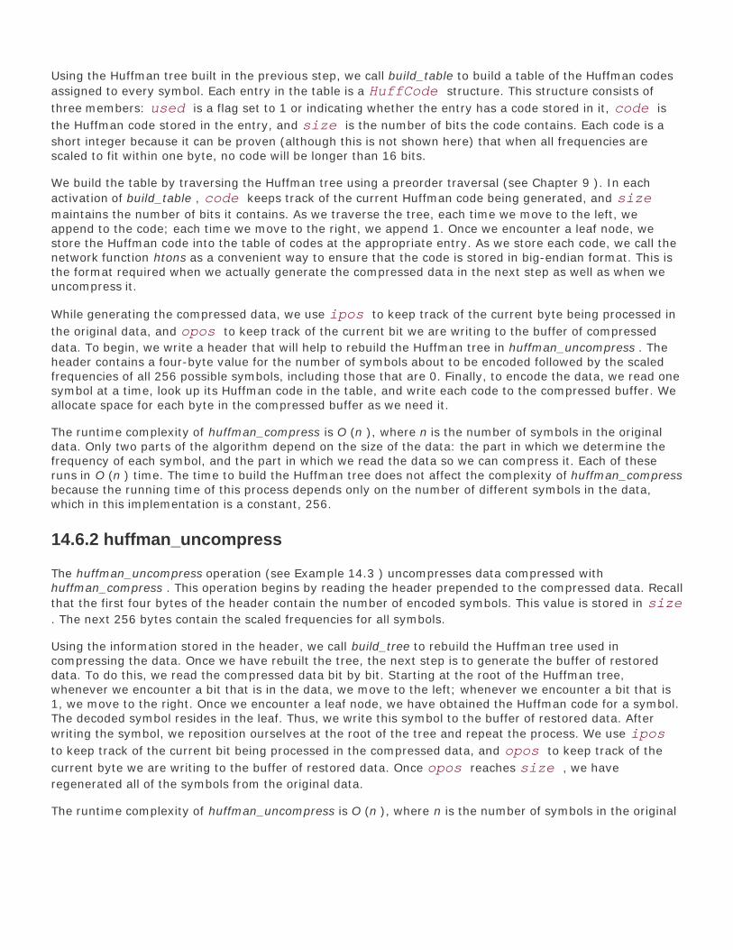
Using the Huffman tree built in the previous step, we call build_table to build a table of the Huffman codes
assigned to every symbol. Each entry in the table is a HuffCode structure. This structure consists of
three members: used is a flag set to 1 or indicating whether the entry has a code stored in it, code is
the Huffman code stored in the entry, and size is the number of bits the code contains. Each code is a
short integer because it can be proven (although this is not shown here) that when all frequencies arescaled to fit within one byte, no code will be longer than 16 bits.
We build the table by traversing the Huffman tree using a preorder traversal (see Chapter 9 ). In each
activation of build_table , code keeps track of the current Huffman code being generated, and sizemaintains the number of bits it contains. As we traverse the tree, each time we move to the left, weappend to the code; each time we move to the right, we append 1. Once we encounter a leaf node, westore the Huffman code into the table of codes at the appropriate entry. As we store each code, we call thenetwork function htons as a convenient way to ensure that the code is stored in big-endian format. This isthe format required when we actually generate the compressed data in the next step as well as when weuncompress it.
While generating the compressed data, we use ipos to keep track of the current byte being processed in
the original data, and opos to keep track of the current bit we are writing to the buffer of compressed
data. To begin, we write a header that will help to rebuild the Huffman tree in huffman_uncompress . Theheader contains a four-byte value for the number of symbols about to be encoded followed by the scaledfrequencies of all 256 possible symbols, including those that are 0. Finally, to encode the data, we read onesymbol at a time, look up its Huffman code in the table, and write each code to the compressed buffer. Weallocate space for each byte in the compressed buffer as we need it.
The runtime complexity of huffman_compress is O (n ), where n is the number of symbols in the originaldata. Only two parts of the algorithm depend on the size of the data: the part in which we determine thefrequency of each symbol, and the part in which we read the data so we can compress it. Each of theseruns in O (n ) time. The time to build the Huffman tree does not affect the complexity of huffman_compressbecause the running time of this process depends only on the number of different symbols in the data,which in this implementation is a constant, 256.
14.6.2 huffman_uncompress
The huffman_uncompress operation (see Example 14.3 ) uncompresses data compressed withhuffman_compress . This operation begins by reading the header prepended to the compressed data. Recall
that the first four bytes of the header contain the number of encoded symbols. This value is stored in size. The next 256 bytes contain the scaled frequencies for all symbols.
Using the information stored in the header, we call build_tree to rebuild the Huffman tree used incompressing the data. Once we have rebuilt the tree, the next step is to generate the buffer of restoreddata. To do this, we read the compressed data bit by bit. Starting at the root of the Huffman tree,whenever we encounter a bit that is in the data, we move to the left; whenever we encounter a bit that is1, we move to the right. Once we encounter a leaf node, we have obtained the Huffman code for a symbol.The decoded symbol resides in the leaf. Thus, we write this symbol to the buffer of restored data. After
writing the symbol, we reposition ourselves at the root of the tree and repeat the process. We use iposto keep track of the current bit being processed in the compressed data, and opos to keep track of the
current byte we are writing to the buffer of restored data. Once opos reaches size , we have
regenerated all of the symbols from the original data.
The runtime complexity of huffman_uncompress is O (n ), where n is the number of symbols in the original

data. This is because for each of the n symbols we decode, the number of levels we must descend in theHuffman tree is a bounded constant that depends on the number of different symbols in the data: in thisimplementation, 256. The time to build the Huffman tree does not affect the complexity ofhuffman_uncompress because this process depends only on the number of different symbols in the data.
Example 14.3. Implementation of Huffman Coding
/****************************************************************************** ** ------------------------------- huffman.c ------------------------------ ** ******************************************************************************/
#include <limits.h>#include <netinet/in.h>#include <stdlib.h>#include <string.h>
#include "bit.h"#include "bitree.h"#include "compress.h"#include "pqueue.h"
/****************************************************************************** ** ----------------------------- compare_freq ----------------------------- ** ******************************************************************************/
static int compare_freq(const void *tree1, const void *tree2) {
HuffNode *root1, *root2;
/****************************************************************************** ** Compare the frequencies stored in the root nodes of two binary trees. ** ******************************************************************************/
root1 = (HuffNode *)bitree_data(bitree_root((const BiTree *)tree1));root2 = (HuffNode *)bitree_data(bitree_root((const BiTree *)tree2));
if (root1->freq < root2->freq) return 1;else if (root1->freq > root2->freq)

return -1;else return 0;
}
/****************************************************************************** ** ----------------------------- destroy_tree ----------------------------- ** ******************************************************************************/
static void destroy_tree(void *tree) {
/****************************************************************************** ** Destroy and free one binary tree from the priority queue of trees. ** ******************************************************************************/
bitree_destroy(tree);free(tree);
return;
}
/****************************************************************************** ** ------------------------------ build_tree ------------------------------ ** ******************************************************************************/
static int build_tree(int *freqs, BiTree **tree) {
BiTree *init, *merge, *left, *right;
PQueue pqueue;
HuffNode *data;
int size, c;

/****************************************************************************** ** Initialize the priority queue of binary trees. ** ******************************************************************************/
*tree = NULL;
pqueue_init(&pqueue, compare_freq, destroy_tree);
for (c = 0; c <= UCHAR_MAX; c++) {
if (freqs[c] != 0) {
/*********************************************************************** * * * Set up a binary tree for the current symbol and its frequency. * * * ***********************************************************************/
if ((init = (BiTree *)malloc(sizeof(BiTree))) == NULL) {
pqueue_destroy(&pqueue); return -1;
}
bitree_init(init, free);
if ((data = (HuffNode *)malloc(sizeof(HuffNode))) == NULL) {
pqueue_destroy(&pqueue); return -1;
}
data->symbol = c; data->freq = freqs[c];
if (bitree_ins_left(init, NULL, data) != 0) {
free(data); bitree_destroy(init); free(init); pqueue_destroy(&pqueue); return -1;
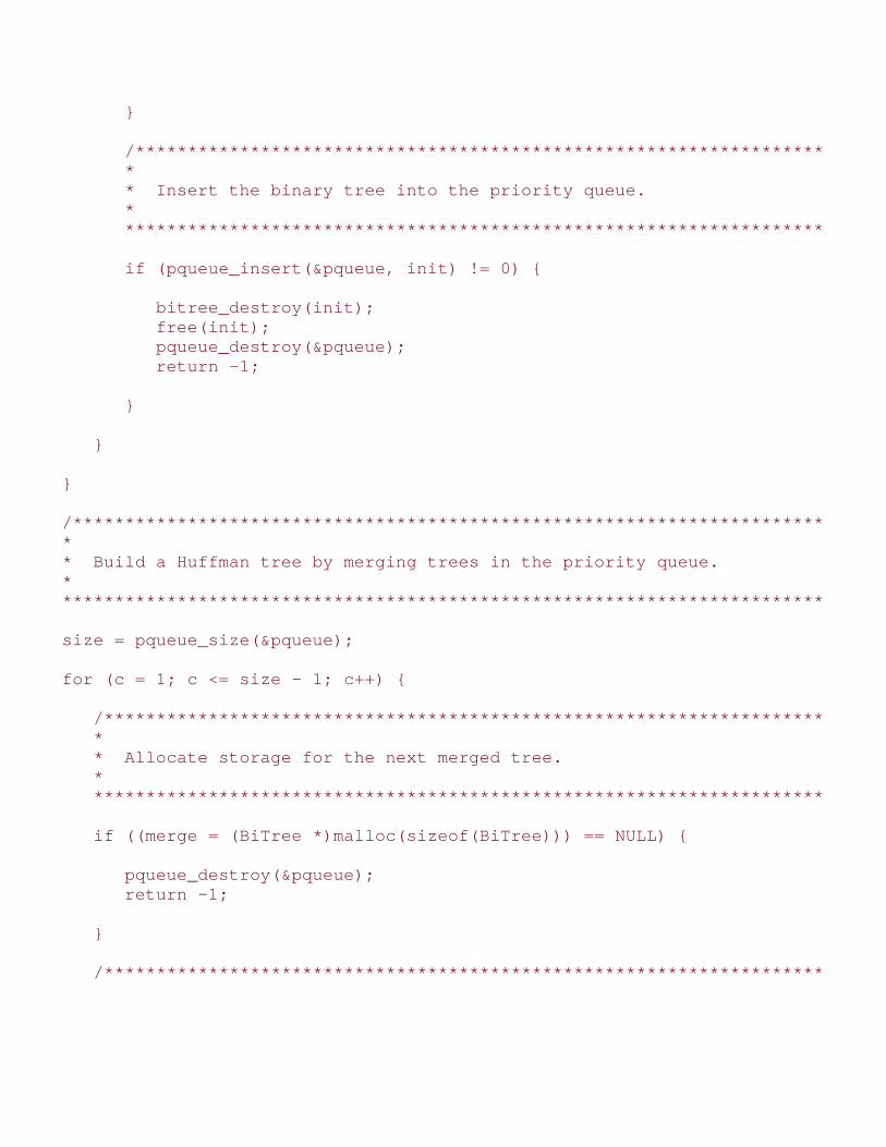
}
/*********************************************************************** * * * Insert the binary tree into the priority queue. * * * ***********************************************************************/
if (pqueue_insert(&pqueue, init) != 0) {
bitree_destroy(init); free(init); pqueue_destroy(&pqueue); return -1;
}
}
}
/****************************************************************************** ** Build a Huffman tree by merging trees in the priority queue. ** ******************************************************************************/
size = pqueue_size(&pqueue);
for (c = 1; c <= size - 1; c++) {
/************************************************************************** * * * Allocate storage for the next merged tree. * * * **************************************************************************/
if ((merge = (BiTree *)malloc(sizeof(BiTree))) == NULL) {
pqueue_destroy(&pqueue); return -1;
}
/**************************************************************************

* * * Extract the two trees whose root nodes have the smallest frequencies. * * * **************************************************************************/
if (pqueue_extract(&pqueue, (void **)&left) != 0) {
pqueue_destroy(&pqueue); free(merge); return -1;
}
if (pqueue_extract(&pqueue, (void **)&right) != 0) {
pqueue_destroy(&pqueue); free(merge); return -1;
}
/************************************************************************** * * * Allocate storage for the data in the root node of the merged tree. * * * **************************************************************************/
if ((data = (HuffNode *)malloc(sizeof(HuffNode))) == NULL) {
pqueue_destroy(&pqueue); free(merge); return -1;
}
memset(data, 0, sizeof(HuffNode));
/************************************************************************** * * * Sum the frequencies in the root nodes of the trees being merged. * * * **************************************************************************/
data->freq = ((HuffNode *)bitree_data(bitree_root(left)))->freq + ((HuffNode *)bitree_data(bitree_root(right)))->freq;

/************************************************************************** * * * Merge the two trees. * * * **************************************************************************/
if (bitree_merge(merge, left, right, data) != 0) {
pqueue_destroy(&pqueue); free(merge); return -1;
}
/************************************************************************** * * * Insert the merged tree into the priority queue and free the others. * * * **************************************************************************/
if (pqueue_insert(&pqueue, merge) != 0) {
pqueue_destroy(&pqueue); bitree_destroy(merge); free(merge); return -1;
}
free(left); free(right);
}
/****************************************************************************** ** The last tree in the priority queue is the Huffman tree. ** ******************************************************************************/
if (pqueue_extract(&pqueue, (void **)tree) != 0) {
pqueue_destroy(&pqueue); return -1;
}

else {
pqueue_destroy(&pqueue);
}
return 0;
}
/****************************************************************************** ** ------------------------------ build_table ----------------------------- ** ******************************************************************************/
static void build_table(BiTreeNode *node, unsigned short code, unsigned char size, HuffCode *table) {
if (!bitree_is_eob(node)) {
if (!bitree_is_eob(bitree_left(node))) {
/*********************************************************************** * * * Move to the left and append 0 to the current code. * * * ***********************************************************************/
build_table(bitree_left(node), code << 1, size + 1, table);
}
if (!bitree_is_eob(bitree_right(node))) {
/*********************************************************************** * * * Move to the right and append 1 to the current code. * * * ***********************************************************************/
build_table(bitree_right(node), (code << 1) | 0x0001, size + 1, table);
}
if (bitree_is_eob(bitree_left(node))&&bitree_is_eob(bitree_right(node))) {

/*********************************************************************** * * * Ensure that the current code is in big-endian format. * * * ***********************************************************************/
code = htons(code);
/*********************************************************************** * * * Assign the current code to the symbol in the leaf node. * * * ***********************************************************************/
table[((HuffNode *)bitree_data(node))->symbol].used = 1; table[((HuffNode *)bitree_data(node))->symbol].code = code; table[((HuffNode *)bitree_data(node))->symbol].size = size;
}
}
return;
}
/****************************************************************************** ** --------------------------- huffman_compress --------------------------- ** ******************************************************************************/
int huffman_compress(const unsigned char *original, unsigned char **compressed, int size) {
BiTree *tree;HuffCode table[UCHAR_MAX + 1];
int freqs[UCHAR_MAX + 1], max, scale, hsize, ipos, opos, cpos,

c, i;
unsigned char *comp, *temp;
/****************************************************************************** ** Initially, there is no buffer of compressed data. ** ******************************************************************************/
*compressed = NULL;
/****************************************************************************** ** Get the frequency of each symbol in the original data. ** ******************************************************************************/
for (c = 0; c <= UCHAR_MAX; c++) freqs[c] = 0;
ipos = 0;
if (size > 0) {
while (ipos < size) {
freqs[original[ipos]]++; ipos++;
}
}
/****************************************************************************** ** Scale the frequencies to fit into one byte. ** ******************************************************************************/
max = UCHAR_MAX;
for (c = 0; c <= UCHAR_MAX; c++) {

if (freqs[c] > max) max = freqs[c];
}
for (c = 0; c <= UCHAR_MAX; c++) {
scale = (int)(freqs[c] / ((double)max / (double)UCHAR_MAX));
if (scale == 0 && freqs[c] != 0) freqs[c] = 1; else freqs[c] = scale;
}
/****************************************************************************** ** Build the Huffman tree and table of codes for the data. ** ******************************************************************************/
if (build_tree(freqs, &tree) != 0) return -1;
for (c = 0; c <= UCHAR_MAX; c++) memset(&table[c], 0, sizeof(HuffCode));
build_table(bitree_root(tree), 0x0000, 0, table);
bitree_destroy(tree);free(tree);
/****************************************************************************** ** Write the header information. ** ******************************************************************************/
hsize = sizeof(int) + (UCHAR_MAX + 1);
if ((comp = (unsigned char *)malloc(hsize)) == NULL) return -1;
memcpy(comp, &size, sizeof(int));

for (c = 0; c <= UCHAR_MAX; c++) comp[sizeof(int) + c] = (unsigned char)freqs[c];
/****************************************************************************** ** Compress the data. ** ******************************************************************************/
ipos = 0;opos = hsize * 8;
while (ipos < size) {
/************************************************************************** * * * Get the next symbol in the original data. * * * **************************************************************************/
c = original[ipos];
/************************************************************************** * * * Write the code for the symbol to the buffer of compressed data. * * * **************************************************************************/
for (i = 0; i < table[c].size; i++) {
if (opos % 8 == 0) {
/******************************************************************** * * * Allocate another byte for the buffer of compressed data. * * * ********************************************************************/
if ((temp = (unsigned char *)realloc(comp,(opos / 8) + 1)) == NULL) {
free(comp); return -1;
}

comp = temp;
}
cpos = (sizeof(short) * 8) - table[c].size + i; bit_set(comp, opos, bit_get((unsigned char *)&table[c].code, cpos)); opos++;
}
ipos++;
}
/****************************************************************************** ** Point to the buffer of compressed data. ** ******************************************************************************/
*compressed = comp;
/****************************************************************************** ** Return the number of bytes in the compressed data. ** ******************************************************************************/
return ((opos - 1) / 8) + 1;
}
/****************************************************************************** ** -------------------------- huffman_uncompress -------------------------- ** ******************************************************************************/
int huffman_uncompress(const unsigned char *compressed, unsigned char **original) {
BiTree *tree;BiTreeNode *node;
int freqs[UCHAR_MAX + 1], hsize,

size, ipos, opos, state, c;
unsigned char *orig, *temp;
/****************************************************************************** ** Initially there is no buffer of original data. ** ******************************************************************************/
*original = orig = NULL;
/****************************************************************************** ** Get the header information from the buffer of compressed data. ** ******************************************************************************/
hsize = sizeof(int) + (UCHAR_MAX + 1);memcpy(&size, compressed, sizeof(int));
for (c = 0; c <= UCHAR_MAX; c++) freqs[c] = compressed[sizeof(int) + c];
/****************************************************************************** ** Rebuild the Huffman tree used previously to compress the data. ** ******************************************************************************/
if (build_tree(freqs, &tree) != 0) return -1;
/****************************************************************************** ** Uncompress the data. ** ******************************************************************************/
ipos = hsize * 8;opos = 0;

node = bitree_root(tree);
while (opos < size) {
/************************************************************************** * * * Get the next bit in the compressed data. * * * **************************************************************************/
state = bit_get(compressed, ipos); ipos++;
if (state == 0) {
/*********************************************************************** * * * Move to the left. * * * ***********************************************************************/
if (bitree_is_eob(node) || bitree_is_eob(bitree_left(node))) {
bitree_destroy(tree); free(tree); return -1;
}
else node = bitree_left(node);
}
else {
/*********************************************************************** * * * Move to the right. * * * ***********************************************************************/
if (bitree_is_eob(node) || bitree_is_eob(bitree_right(node))) {
bitree_destroy(tree); free(tree);

return -1;
}
else node = bitree_right(node);
}
if (bitree_is_eob(bitree_left(node))&&bitree_is_eob(bitree_right(node))) {
/*********************************************************************** * * * Write the symbol in the leaf node to the buffer of original data. * * * ***********************************************************************/
if (opos > 0) {
if ((temp = (unsigned char *)realloc(orig, opos + 1)) == NULL) {
bitree_destroy(tree); free(tree); free(orig); return -1;
}
orig = temp;
}
else {
if ((orig = (unsigned char *)malloc(1)) == NULL) {
bitree_destroy(tree); free(tree); return -1;
}
}
orig[opos] = ((HuffNode *)bitree_data(node))->symbol; opos++;

/*********************************************************************** * * * Move back to the top of the tree. * * * ***********************************************************************/
node = bitree_root(tree);
}
}
bitree_destroy(tree);free(tree);
/****************************************************************************** ** Point to the buffer of original data. ** ******************************************************************************/
*original = orig;
/****************************************************************************** ** Return the number of bytes in the original data. ** ******************************************************************************/
return opos;
}
Top

Mastering Algorithms with CBy Kyle LoudonSlots : 1Table of ContentsChapter 14. Data Compression
Content
14.7 Huffman Coding Example: Optimized Networking
Transferring data across a network can be a time-consuming process, particularly across slow wide-areanetworks. One approach to managing this problem is to compress the data before sending it and thenuncompress it when it is received. Although sometimes the time spent compressing and uncompressingdata may not be worth the savings in time across the network, in many network applications this cost iswell justified. This example presents two functions, send_comp and recv_comp (see Example 14.4 ), thatsend and receive data in a compressed format.
The send_comp function sends data by first compressing it and then calling the standard socket function
send . To send the data, send_comp requires four arguments: s is a socket descriptor for which a
connection has already been established, data is the buffer of data to send, size is the size of the data,
and flags is the normal flags argument passed to send . To begin the sending process, we compress
the data in data by calling huffman_compress . Next, we send the size of the compressed data, as
returned by huffman_compress , so that space can be allocated on the receiving end. This is part of asimple protocol we establish with the receiver. Last, we send the compressed data itself and then free it asthe interface to huffman_compress suggests.
The recv_comp function uses the standard socket function recv to receive data sent by send_comp . To
receive the data, recv_comp requires four arguments: s is a socket descriptor for which a connection has
already been established, data is a pointer that recv_comp will set to the uncompressed data, size is
the size of the data as set by recv_comp on return, and flags is the normal flags argument passed to
recv . To begin the receiving process, we receive the size of the data and allocate a buffer. Next, we receivethe compressed data and call huffman_uncompress to uncompress it. Since huffman_uncompressdynamically allocates space for the uncompressed data using malloc , and recv_comp returns this pointer,it is the responsibility of the caller of recv_comp to call free when the data is no longer needed. Last, wefree the buffer we allocated to receive the data.
The runtime complexities of send_comp and recv_comp are both O (n ), where n is the number of symbolssent or received. These complexities are both O (n ) because the two functions call huffman_compress andhuffman_uncompress respectively, which are both O (n ) operations.

Example 14.4. Implementation of Functions for Optimized Networking
/****************************************************************************** ** ------------------------------ transfer.c ------------------------------ ** ******************************************************************************/
#include <sys/types.h>#include <sys/socket.h>
#include "compress.h"#include "transfer.h"
/****************************************************************************** ** ------------------------------- send_comp ------------------------------ ** ******************************************************************************/
int send_comp(int s, const unsigned char *data, int size, int flags) {
unsigned char *compressed;
int size_comp;
/****************************************************************************** ** Compress the data. ** ******************************************************************************/
if ((size_comp = huffman_compress(data, &compressed, size)) < 0) return -1;
/****************************************************************************** ** Send the compressed data preceded by its size. ** ******************************************************************************/
if (send(s, (char *)&size_comp, sizeof(int), flags) != sizeof(int)) return -1;
if (send(s, (char *)compressed, size_comp, flags) != size_comp) return -1;

/****************************************************************************** ** Free the buffer of compressed data. ** ******************************************************************************/
free(compressed);
return 0;
}
/****************************************************************************** ** ------------------------------- recv_comp ------------------------------ ** ******************************************************************************/
int recv_comp(int s, unsigned char **data, int *size, int flags) {
unsigned char *compressed;
int size_comp;
/****************************************************************************** ** Receive the compressed data preceded by its size. ** ******************************************************************************/
if (recv(s, (char *)&size_comp, sizeof(int), flags) != sizeof(int)) return -1;
if ((compressed = (unsigned char *)malloc(size_comp)) == NULL) return -1;
if (recv(s, (char *)compressed, size_comp, flags) != size_comp) {
free(compressed); return -1;
}
/****************************************************************************** *

* Uncompress the data. ** ******************************************************************************/
if ((*size = huffman_uncompress(compressed, data)) < 0) return -1;
/****************************************************************************** ** Free the buffer of compressed data. ** ******************************************************************************/
free(compressed);
return 0;
}
Top

Mastering Algorithms with CBy Kyle Loudon
Slots : 1
Table of Contents
Chapter 14. Data Compression
Content
14.8 Description of LZ77
LZ77 ( Lempel-Ziv-1977) is a simple but surprisingly effective form of data compression that takesan entirely different approach from Huffman coding. LZ77 is a dictionary-based method, which meansthat it tries to compress data by encoding long strings of symbols, called phrases, as small tokensthat reference entries in a dictionary. Compression is achieved by using relatively small tokens inplace of longer phrases that appear several times in the data. As with Huffman coding, it is importantto realize that a symbol is not necessarily a character of text: a symbol can be any amount of datawe choose, but it is often one byte's worth.
14.8.1 Maintaining a Dictionary of Phrases
Different dictionary-based compression methods use various approaches for maintaining theirdictionaries. LZ77 uses a look-ahead buffer and a sliding window. LZ77 works by first loading aportion of the data into the look-ahead buffer. To understand how the look-ahead buffer storesphrases that effectively form a dictionary, picture the buffer as a sequence of symbols s1, . . . , sn,and Pb as a set of phrases constructed from the symbols. From the sequence s1, . . . , sn, we form nphrases, defined as:
Pb = {(s1), (s1, s2), . . . ,(s1, . . . ,sn)}
This means that if the look-ahead buffer contains the symbols (A, B, D), for example, the phrases inthe buffer are {(A), (A, B), (A, B, D)}. Once data passes through the look-ahead buffer, it movesinto the sliding window and becomes part of the dictionary. To understand how phrases arerepresented in the sliding window, consider the window to be a sequence of symbols s1, . . ., sm, andPw to be a set of phrases constructed from these symbols. From the sequence s1, . . ., sm, we formthe set of phrases as follows:
Pw = {p1, p2, . . . , pm}, where pi = {(si), (si, si+1), . . . , si, si+1, . . . , sm)}
Thus, if the sliding window contains the symbols (A, B, C), the phrases in the window, and hence thedictionary, are {(A), (A, B), (A, B, C), (B), (B, C), (C)}. The main idea behind LZ77 is to lookcontinually for the longest phrase in the look-ahead buffer that matches a phrase currently in thedictionary. In the look-ahead buffer and sliding window just described, the longest match is the two-symbol phrase (A, B).

14.8.2 Compressing and Uncompressing Data
As we compress the data, two situations can exist between the look-ahead buffer and the slidingwindow at any given moment: there can either be a phrase of some length that matches, or theremay be no match at all. When there is at least one match, we encode the longest match as a phrasetoken. Phrase tokens contain three pieces of information: the offset in the sliding window where thematch begins, the number of symbols in the match, and the first symbol in the look-ahead bufferafter the match. When there is no match, we encode the unmatched symbol as a symbol token.Symbol tokens simply contain the unmatched symbol itself, so no compression is accomplished. Infact, we will see that symbol tokens actually contain one bit more than the symbol itself, so a slightexpansion occurs.
Once the appropriate token has been generated that encodes some number of symbols n, we shift nsymbols out one end of the sliding window and replace them at the other end by the same number ofsymbols shifted out of the look-ahead buffer. Next, we refill the look-ahead buffer. This processkeeps the sliding window up to date with only the most recent phrases. The exact number of phrasesmaintained by the sliding window and look-ahead buffer depends on their size.
Figure 14.2 illustrates the compression of a string using LZ77 with a sliding window of 8 bytes and alook-ahead buffer of 4 bytes. In practice, typical sizes for sliding windows are around 4K (4096bytes). Look-ahead buffers are generally less than 100 bytes.
Figure 14.2. Compressing the string ABABCBABABCAD using LZ77
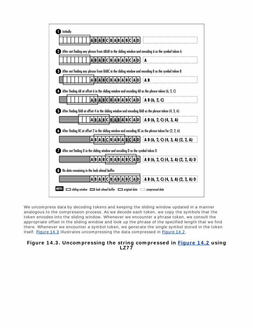
We uncompress data by decoding tokens and keeping the sliding window updated in a manneranalogous to the compression process. As we decode each token, we copy the symbols that thetoken encodes into the sliding window. Whenever we encounter a phrase token, we consult theappropriate offset in the sliding window and look up the phrase of the specified length that we findthere. Whenever we encounter a symbol token, we generate the single symbol stored in the tokenitself. Figure 14.3 illustrates uncompressing the data compressed in Figure 14.2.
Figure 14.3. Uncompressing the string compressed in Figure 14.2 usingLZ77

14.8.3 Effectiveness of LZ77
The amount of compression achieved using LZ77 depends on a number of factors, such as the sizechosen for the sliding window, the size set for the look-ahead buffer, and the entropy of the dataitself. Ultimately, the amount of compression depends on the number of phrases we are able tomatch and their lengths. In most cases, LZ77 results in better compression ratios than Huffmancoding, but compression times are considerably slower.
Compressing data with LZ77 is time-consuming because we spend a lot of time searching the slidingwindow for matching phrases. However, in general, uncompressing data with LZ77 is even fasterthan ucompressing data with Huffman coding. Uncompressing data with LZ77 is fast because eachtoken tells us exactly where to read symbols out of the buffer. In fact, we end up reading from thesliding window only as many symbols as in the original data.
Top

Mastering Algorithms with CBy Kyle LoudonSlots : 1Table of ContentsChapter 14. Data Compression
Content
14.9 Interface for LZ77lz77_compress
int lz77_compress(const unsigned char *original, unsigned char **compressed, int size);
Return Value
Number of bytes in the compressed data if compressing the data is successful, or -1 otherwise.
Description
Uses LZ77 to compress a buffer of data specified by original , which contains size bytes. The
compressed data is written to a buffer returned in compressed . Since the amount of storage required in
compressed is unknown to the caller, lz77_compress dynamically allocates the necessary storage using
malloc . It is the responsibility of the caller to free this storage using free when it is no longer needed.
Complexity
O (n ), where n is the number of symbols in the original data.
lz77_uncompress
int lz77_uncompress(const unsigned char *compressed, unsigned char **original);
Return Value

Number of bytes in the restored data if uncompressing the data is successful, or -1 otherwise.
Description
Uses LZ77 to uncompress a buffer of data specified by compressed . It is assumed that the buffer
contains data previously compressed with lz77_compress . The restored data is written to a buffer returned
in original . Since the amount of storage required in original may not be known to the caller,
lz77_uncompress dynamically allocates the necessary storage using malloc . It is the responsibility of thecaller to free this storage using free when it is no longer needed.
Complexity
O (n ), where n is the number of symbols in the original data.
Top

Mastering Algorithms with CBy Kyle LoudonSlots : 1Table of ContentsChapter 14. Data Compression
Content
14.10 Implementation and Analysis of LZ77
With LZ77, we try to compress data by encoding phrases from a look-ahead buffer as tokens referencingphrases in a sliding window. To uncompress the data, we decode each token into the phrase or symbol itrepresents. To do this, we must continually update the sliding window so that at any one time it looks thesame as it did during the compression process. In the implementation presented here, a symbol in theoriginal data is one byte.
14.10.1 lz77_compress
The lz77_compress operation (see Example 14.5 ) compresses data using LZ77. It begins by writing thenumber of symbols in the data to the buffer of compressed data and initializing the sliding window andlook-ahead buffer. The look-ahead buffer is then loaded with symbols.
Compression takes place inside of a loop that iterates until there are no more symbols to process. We use
ipos to keep track of the current byte being processed in the original data, and opos to keep track of
the current bit we are writing to the buffer of compressed data. During each iteration of the loop, we callcompare_win to determine the longest phrase in the look-ahead buffer that matches one in the slidingwindow. The compare_win function returns the length of the longest match.
When a match is found, compare_win sets offset to the position of the match in the sliding window and
next to the symbol in the look-ahead buffer immediately after the match. In this case, we write a phrase
token to the compressed data (see Figure 14.4 a). Phrase tokens in the implementation presented hererequire 12 bits for offsets because the size of the sliding window is 4K (4096 bytes). Phrase tokens require5 bits for lengths because no match will exceed the length of the look-ahead buffer, which is 32 bytes. If a
match is not found, compare_win returns and sets next to the unmatched symbol at the start of the
look-ahead buffer. In this case, we write a symbol token to the compressed data (see Figure 14.4 b).Whether we write a phrase or symbol token to the compressed data, before actually writing the token, wecall the network function htonl as a convenient way to ensure that the token is in big-endian format. This isthe format required when we actually store the compressed data as well as when we uncompress it.

Figure 14.4. The structure of (a) a phrase token and (b) a symbol token inLZ77
Once we write the appropriate token to the buffer of compressed data, we adjust the sliding window andthe look-ahead buffer. To move the data through the sliding window, we shift data in from the right side ofthe window and out the left. We do the same for the look-ahead buffer. The number of bytes we move isequal to the number of symbols we encode in the token.
The runtime complexity of lz77_compress is O (n ), where n is the number of symbols in the original data.This is because for each of the n /c tokens in which the data is encoded, where 1/c is a constant factor thatrepresents how efficiently symbols are encoded in phrase tokens, we call compare_win once. Thecompare_win function runs in a constant amount of time because the size of the sliding window and look-ahead buffer are both constant. However, these constants are large and contribute significantly to theoverall running time of lz77_compress . Thus, the runtime complexity of lz77_compress is O (n ), but itsactual running time is greatly affected by constant factors. This explains the generally slow performance ofLZ77 when compressing data.
14.10.2 lz77_uncompress
The lz77_uncompress operation (see Figure 14.4 ) uncompresses data previously compressed withlz77_compress . It begins by reading the number of symbols in the compressed data and initializing thesliding window and look-ahead buffer.
Uncompressing the data takes place inside a loop that iterates until there are no more symbols to process.
We use ipos to keep track of the current bit being processed in the compressed data, and opos to keep
track of the current byte we are writing to the buffer of restored data. During each iteration of the loop, wefirst read one bit from the compressed data to determine the type of token we are about to decode.
At the start of interpreting a token, if the first bit read is 1, we have encountered a phrase token . Thus, weread each of its members, look up the phrase in the sliding window, and write the phrase to the buffer ofrestored data. As we look up each phrase, we call the network function ntohl to ensure that the byteordering of its offset and length in the window are correct for the system. This step is required becauseboth the offset and length are in big-endian format when read from the compressed data. The look-aheadbuffer is used as a convenient place to temporarily store the data before copying it into the sliding window.Last, we write the unmatched symbol encoded by the token. If the first bit read for the token is 0, we haveencountered a symbol token. In this case, we write the one unmatched symbol it encodes to the buffer ofrestored data.
Once we write the decoded data to the buffer of restored data, we adjust the sliding window. To move thedata through the sliding window, we shift the decoded data in from the right side of the window and out the

left. The number of bytes we move is equal to the number of symbols we decode from the token.
The runtime complexity of lz77_uncompress is O (n ), where n is the number of symbols in the originaldata. This is because for each of the n /c tokens in which the data is encoded, where 1/c is a constantfactor that represents how efficiently symbols are encoded in phrase tokens , we perform the constant-timeoperation of copying symbols from the sliding window to the buffer of restored data. Thus, the runtimecomplexity of lz77_uncompress is O (n ). Its lack of significant constant factors explains its generallysuperior performance to huffman_uncompress and its vast improvement in actual running time overlz77_compress .
Example 14.5. Implementation of LZ77
/****************************************************************************** ** -------------------------------- lz77.c -------------------------------- ** ******************************************************************************/
#include <netinet/in.h>#include <stdlib.h>#include <string.h>
#include "bit.h"#include "compress.h"
/****************************************************************************** ** ------------------------------ compare_win ----------------------------- ** ******************************************************************************/
static int compare_win(const unsigned char *window, const unsigned char *buffer, int *offset, unsigned char *next) {
int match, longest, i, j, k;
/****************************************************************************** ** Initialize the offset, although it is valid only once a match is found. ** ******************************************************************************/
*offset = 0;

/****************************************************************************** ** If no match is found, prepare to return 0 and the next symbol in the ** look-ahead buffer. ** ******************************************************************************/
longest = 0;*next = buffer[0];
/****************************************************************************** ** Look for the best match in the look-ahead buffer and sliding window. ** ******************************************************************************/
for (k = 0; k < LZ77_WINDOW_SIZE; k++) {
i = k; j = 0; match = 0;
/************************************************************************** * * * Determine how many symbols match in the sliding window at offset k. * * * **************************************************************************/
while (i < LZ77_WINDOW_SIZE && j < LZ77_BUFFER_SIZE - 1) {
if (window[i] != buffer[j]) break;
match++; i++; j++;
}
/************************************************************************** * * * Keep track of the offset, length, and next symbol for the best match. * * * **************************************************************************/
if (match > longest) {

*offset = k; longest = match; *next = buffer[j];
}
}
return longest;
}
/****************************************************************************** ** ----------------------------- lz77_compress ---------------------------- ** ******************************************************************************/
int lz77_compress(const unsigned char *original, unsigned char **compressed, int size) {
unsigned char window[LZ77_WINDOW_SIZE], buffer[LZ77_BUFFER_SIZE], *comp, *temp, next;
int offset, length, remaining, hsize, ipos, opos, tpos, i;
/****************************************************************************** ** Make the pointer to the compressed data not valid until later. ** ******************************************************************************/
*compressed = NULL;
/*****************************************************************************
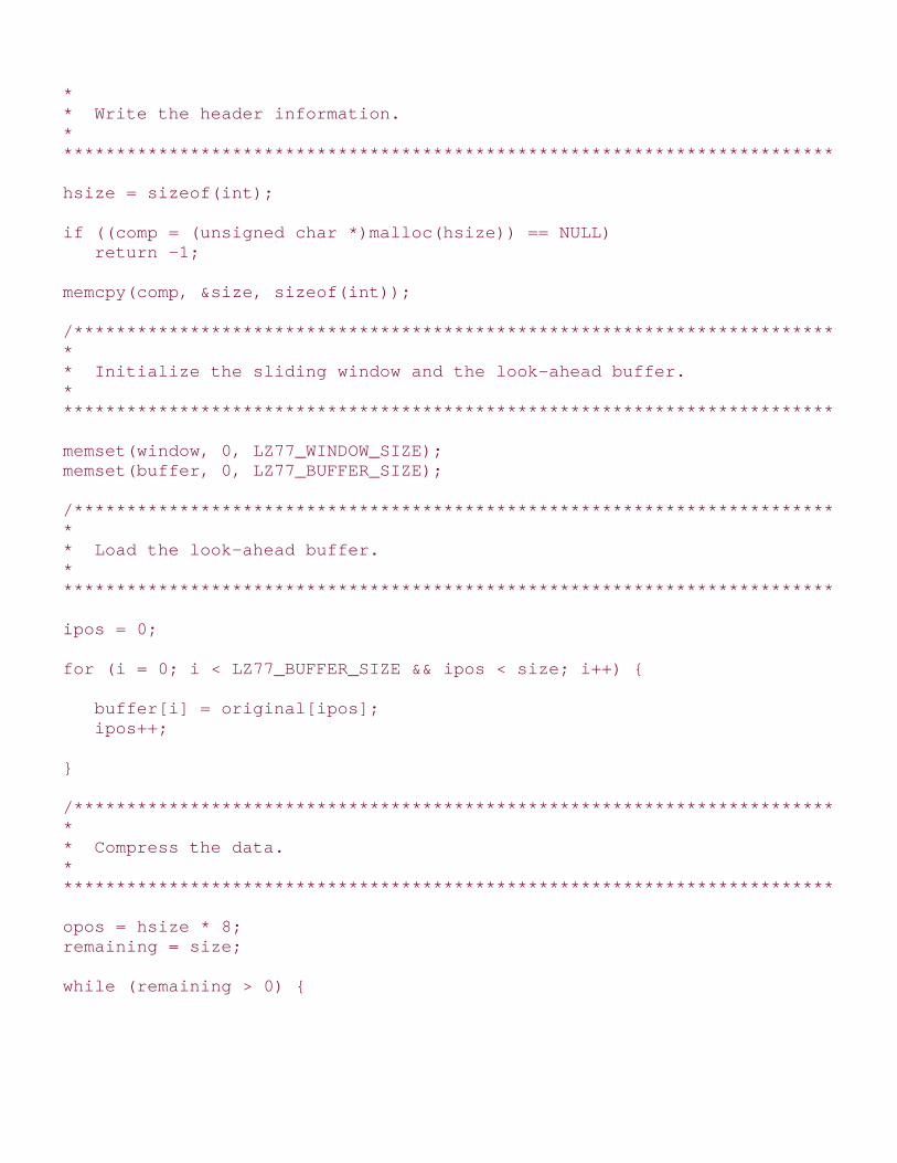
* ** Write the header information. ** ******************************************************************************/
hsize = sizeof(int);
if ((comp = (unsigned char *)malloc(hsize)) == NULL) return -1;
memcpy(comp, &size, sizeof(int));
/****************************************************************************** ** Initialize the sliding window and the look-ahead buffer. ** ******************************************************************************/
memset(window, 0, LZ77_WINDOW_SIZE);memset(buffer, 0, LZ77_BUFFER_SIZE);
/****************************************************************************** ** Load the look-ahead buffer. ** ******************************************************************************/
ipos = 0;
for (i = 0; i < LZ77_BUFFER_SIZE && ipos < size; i++) {
buffer[i] = original[ipos]; ipos++;
}
/****************************************************************************** ** Compress the data. ** ******************************************************************************/
opos = hsize * 8;remaining = size;
while (remaining > 0) {
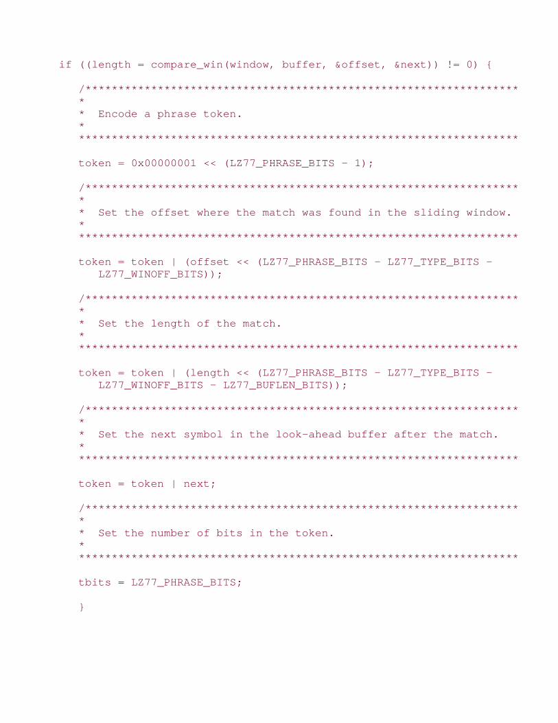
if ((length = compare_win(window, buffer, &offset, &next)) != 0) {
/*********************************************************************** * * * Encode a phrase token. * * * ***********************************************************************/
token = 0x00000001 << (LZ77_PHRASE_BITS - 1);
/*********************************************************************** * * * Set the offset where the match was found in the sliding window. * * * ***********************************************************************/
token = token | (offset << (LZ77_PHRASE_BITS - LZ77_TYPE_BITS - LZ77_WINOFF_BITS));
/*********************************************************************** * * * Set the length of the match. * * * ***********************************************************************/
token = token | (length << (LZ77_PHRASE_BITS - LZ77_TYPE_BITS - LZ77_WINOFF_BITS - LZ77_BUFLEN_BITS));
/*********************************************************************** * * * Set the next symbol in the look-ahead buffer after the match. * * * ***********************************************************************/
token = token | next;
/*********************************************************************** * * * Set the number of bits in the token. * * * ***********************************************************************/
tbits = LZ77_PHRASE_BITS; }
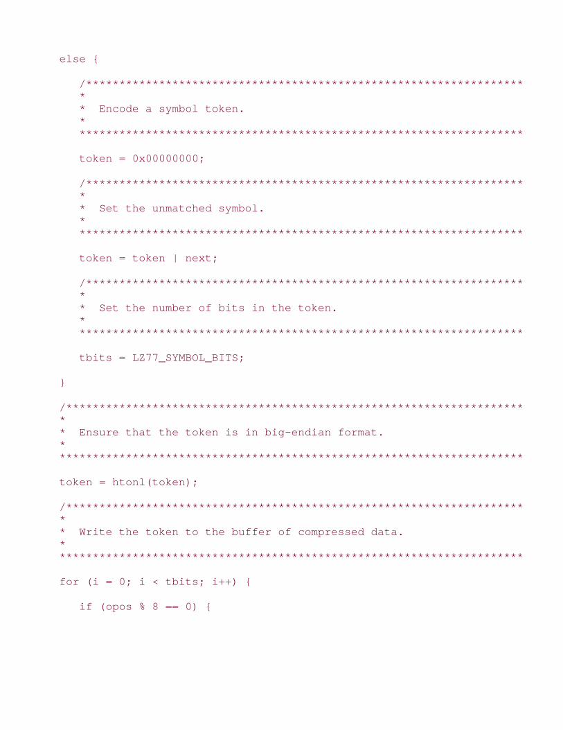
else {
/*********************************************************************** * * * Encode a symbol token. * * * ***********************************************************************/
token = 0x00000000;
/*********************************************************************** * * * Set the unmatched symbol. * * * ***********************************************************************/
token = token | next;
/*********************************************************************** * * * Set the number of bits in the token. * * * ***********************************************************************/
tbits = LZ77_SYMBOL_BITS;
}
/************************************************************************** * * * Ensure that the token is in big-endian format. * * * **************************************************************************/
token = htonl(token);
/************************************************************************** * * * Write the token to the buffer of compressed data. * * * **************************************************************************/
for (i = 0; i < tbits; i++) {
if (opos % 8 == 0) {

/******************************************************************** * * * Allocate another byte for the buffer of compressed data. * * * ********************************************************************/
if ((temp = (unsigned char *)realloc(comp,(opos / 8) + 1)) == NULL) {
free(comp); return -1;
}
comp = temp;
}
tpos = (sizeof(unsigned long) * 8) - tbits + i; bit_set(comp, opos, bit_get((unsigned char *)&token, tpos)); opos++;
}
/************************************************************************** * * * Adjust the phrase length to account for the unmatched symbol. * * * **************************************************************************/
length++; /************************************************************************** * * * Copy data from the look-ahead buffer to the sliding window. * * * **************************************************************************/
memmove(&window[0], &window[length], LZ77_WINDOW_SIZE - length); memmove(&window[LZ77_WINDOW_SIZE - length], &buffer[0], length);
/************************************************************************** * * * Read more data into the look-ahead buffer. * * * **************************************************************************/

memmove(&buffer[0], &buffer[length], LZ77_BUFFER_SIZE - length);
for (i = LZ77_BUFFER_SIZE - length; i<LZ77_BUFFER_SIZE && ipos<size; i++) {
buffer[i] = original[ipos]; ipos++;
}
/************************************************************************** * * * Adjust the total symbols remaining by the phrase length. * * * **************************************************************************/
remaining = remaining - length;
}
/****************************************************************************** ** Point to the buffer of compressed data. ** ******************************************************************************/
*compressed = comp;
/****************************************************************************** ** Return the number of bytes in the compressed data. ** ******************************************************************************/
return ((opos - 1) / 8) + 1;
}
/****************************************************************************** ** ---------------------------- lz77_uncompress --------------------------- ** ******************************************************************************/
int lz77_uncompress(const unsigned char *compressed, unsigned char **original) {

unsigned char window[LZ77_WINDOW_SIZE], buffer[LZ77_BUFFER_SIZE], *orig, *temp, next;
int offset, length, remaining, hsize, size, ipos, opos, tpos, state, i;
/****************************************************************************** ** Make the pointer to the original data not valid until later. ** ******************************************************************************/
*original = orig = NULL;
/****************************************************************************** ** Get the header information. ** ******************************************************************************/
hsize = sizeof(int);memcpy(&size, compressed, sizeof(int));
/****************************************************************************** ** Initialize the sliding window and the look-ahead buffer. ** ******************************************************************************/
memset(window, 0, LZ77_WINDOW_SIZE);memset(buffer, 0, LZ77_BUFFER_SIZE);
/****************************************************************************** ** Uncompress the data. *

* ******************************************************************************/
ipos = hsize * 8;opos = 0;remaining = size;
while (remaining > 0) {
/************************************************************************** * * * Get the next bit in the compressed data. * * * **************************************************************************/
state = bit_get(compressed, ipos); ipos++;
if (state == 1) {
/*********************************************************************** * * * Handle processing a phrase token. * * * ***********************************************************************/
memset(&offset, 0, sizeof(int));
for (i = 0; i < LZ77_WINOFF_BITS; i++) {
tpos = (sizeof(int) * 8) - LZ77_WINOFF_BITS + i; bit_set((unsigned char *)&offset, tpos, bit_get(compressed, ipos)); ipos++;
}
memset(&length, 0, sizeof(int));
for (i = 0; i < LZ77_BUFLEN_BITS; i++) {
tpos = (sizeof(int) * 8) - LZ77_BUFLEN_BITS + i; bit_set((unsigned char *)&length, tpos, bit_get(compressed, ipos)); ipos++;
}

next = 0x00;
for (i = 0; i < LZ77_NEXT_BITS; i++) {
tpos = (sizeof(unsigned char) * 8) - LZ77_NEXT_BITS + i; bit_set((unsigned char *)&next, tpos, bit_get(compressed, ipos)); ipos++;
}
/*********************************************************************** * * * Ensure that the offset and length have the correct byte ordering * * for the system. * * * ***********************************************************************/
offset = ntohl(offset); length = ntohl(length);
/*********************************************************************** * * * Write the phrase from the window to the buffer of original data. * * * ***********************************************************************/
i = 0;
if (opos > 0) {
if ((temp = (unsigned char *)realloc(orig, opos+length+1)) == NULL) {
free(orig); return -1;
}
orig = temp;
}
else {
if ((orig = (unsigned char *)malloc(length + 1)) == NULL) return -1;

}
while (i < length && remaining > 0) {
orig[opos] = window[offset + i]; opos++;
/******************************************************************** * * * Record each symbol in the look-ahead buffer until ready to * * update the sliding window. * * * ********************************************************************/
buffer[i] = window[offset + i]; i++;
/******************************************************************** * * * Adjust the total symbols remaining to account for each symbol * * consumed. * * * ********************************************************************/
remaining--;
}
/*********************************************************************** * * * Write the unmatched symbol to the buffer of original data. * * * ***********************************************************************/
if (remaining > 0) {
orig[opos] = next; opos++;
/******************************************************************** * * * Also record this symbol in the look-ahead buffer. * * * ********************************************************************/
buffer[i] = next;

/******************************************************************** * * * Adjust the total symbols remaining to account for the unmatched * * symbol. * * * ********************************************************************/
remaining--;
}
/*********************************************************************** * * * Adjust the phrase length to account for the unmatched symbol. * * * ***********************************************************************/
length++;
}
else {
/*********************************************************************** * * * Handle processing a symbol token. * * * ***********************************************************************/
next = 0x00;
for (i = 0; i < LZ77_NEXT_BITS; i++) {
tpos = (sizeof(unsigned char) * 8) - LZ77_NEXT_BITS + i; bit_set((unsigned char *)&next, tpos, bit_get(compressed, ipos)); ipos++;
}
/*********************************************************************** * * * Write the symbol to the buffer of original data. * * * ***********************************************************************/

if (opos > 0) {
if ((temp = (unsigned char *)realloc(orig, opos + 1)) == NULL) {
free(orig); return -1;
}
orig = temp;
}
else {
if ((orig = (unsigned char *)malloc(1)) == NULL) return -1;
}
orig[opos] = next; opos++;
/*********************************************************************** * * * Record the symbol in the look-ahead buffer until ready to update * * the sliding window. * * * ***********************************************************************/
if (remaining > 0) buffer[0] = next;
/*********************************************************************** * * * Adjust the total symbols remaining to account for the unmatched * * symbol. * * * ***********************************************************************/
remaining--;
/*********************************************************************** * * * Set the phrase length to account for the unmatched symbol. * * *

***********************************************************************/
length = 1;
}
/************************************************************************** * * * Copy the look-ahead buffer into the sliding window. * * * **************************************************************************/
memmove(&window[0], &window[length], LZ77_WINDOW_SIZE - length); memmove(&window[LZ77_WINDOW_SIZE - length], &buffer[0], length);
}
/****************************************************************************** ** Point to the buffer of original data. ** ******************************************************************************/
*original = orig;
/****************************************************************************** ** Return the number of bytes in the original data. ** ******************************************************************************/
return opos;
}
Top

Mastering Algorithms with CBy Kyle Loudon
Slots : 1
Table of Contents
Chapter 14. Data Compression
Content
14.11 Questions and Answers
Q: There are certain cases where compressing data may generate poor results. When might weencounter this with Huffman coding?
A: Effective compression with Huffman coding depends on symbols occurring in the data at varyingfrequencies. If all possible symbols occur at nearly the same frequency, poor compression results.Huffman coding also performs poorly when used to compress small amounts of data. In this case, thespace required by the table in the header negates the compression achieved in the data. Fortunately,these limitations are not normally a problem because the symbols in most data are not uniformlydistributed, and we are usually not interested in compressing small amounts of data.
Q: Just as with Huffman coding, there are certain cases in which LZ77 achieves poor compression.What are some of these cases?
A: Effective compression with LZ77 depends on being able to encode many sequences of symbolsusing phrase tokens. If we generate a large number of symbol tokens and only a few phrase tokensrepresenting predominantly short phrases, poor compression results. An excessive number of symboltokens may even cause the compressed data to be larger than the original data itself. This occurswhen the sliding window is made too small to take advantage of recurring phrases effectively.
Q: In the implementation of both Huffman coding and LZ77 presented in this chapter, the end of thecompressed data is recognized by counting symbols. This means we must store a symbol count alongwith the compressed data itself. What is another approach to recognizing the end of the data? Whatimpact would this have on each implementation?
A: When uncompressing data, we must have a way to determine exactly where the data ends. Analternative to storing a symbol count is to encode a special end-of-data symbol. In theimplementations in this chapter, this would mean encoding 257 symbols instead of 256. To accountfor this with Huffman coding, we need only make the symbol member of the HuffNode structure ashort integer instead of an unsigned character. Thus, the size of the compressed data is affected verylittle. On the other hand, in the implementation of LZ77, without substantial changes to the way weinterpret tokens, we would need to store an extra bit with each token to represent the 257 possiblesymbols. Thus, the size of the compressed data would increase, making this method less effectivethan simply counting symbols.
Q: With LZ77, what factors must be balanced in selecting the size of the sliding window? What factorsmust be balanced in selecting the size of the look-ahead buffer?

A: Recall that the implementation of LZ77 presented in this chapter used a sliding window 4K (4096bytes) in size and a look-ahead buffer of 32 bytes, which are common choices. The size of the slidingwindow determines how far back in the data we search for matching phrases. Generally, it is a goodidea to search quite far back to allow a good opportunity for matches. However, we must balance thisagainst the time it takes to search through the sliding window. Also, we must balance this against thespace penalty of using more bits for offsets in phrase tokens. The size we choose for the look-aheadbuffer determines the maximum length of phrases we can match. If the data has many long phrasesthat are duplicated, choosing a buffer size that is too small results in multiple phrase tokens wherewe might otherwise get just one. However, we must balance this against the space penalty of usingmore bits for lengths in phrase tokens.
Q: In Huffman coding, how might we decrease the space required by the header at the front ofcompressed data? Are there any problems associated with this?
A: Recall that in the implementation of Huffman coding presented in this chapter a header wasprepended to the compressed data. This header contained a table of 256 entries, one entry for eachpossible symbol. If several symbols have frequencies of 0, this is somewhat wasteful. For example,when compressing ASCII text, many symbols are not used, so their frequencies are 0. A betterapproach to storing the table in this case is to use count runs. A count run consists of the value of astarting symbol c followed by a length l. It tells us that the next l entries in the table will be entriesfor the symbols c, c + 1, . . ., c + l - 1. In many cases, this reduces the size of the table. However,when the table is nearly full to begin with, it actually increases the table size slightly.
Q: One of the most costly aspects of LZ77 is scanning the sliding window for matching phrases. Howcan we improve the performance of this?
A: LZ77 looks for matching phrases by comparing portions of the sliding window to portions of thelook-ahead buffer essentially symbol by symbol. A more effective approach is to replace the slidingwindow with some type of data structure for efficient searching. For example, we might use a hashtable (see Chapter 8) or a binary search tree (see Chapter 9) to store phrases encountered earlier.In fact, this is the approach employed by several more efficient variations of LZ77 (see the relatedtopics at the end of the chapter).
Q: Considering the performance differences and compression normally achieved by Huffman codingand LZ77, when might we use one over the other?
A: LZ77 generally results in better compression than Huffman coding, but with a significantperformance penalty during the compression process. One situation in which this might not pose aproblem is the distribution of large software packages. LZ77 works well here because the data onlyneeds to be compressed once (at the production facility), and clients benefit from the considerablyfaster operation of uncompressing the data. On the other hand, suppose we are sending largeamounts of data across a network interactively and would like to compress it before eachtransmission. In this case, for every transmission, we must compress data on one end of theconnection and uncompress it on the other. Therefore, it is best to use Huffman coding. We may notachieve as much compression as with LZ77, but compressing and uncompressing together are faster.
Top

Mastering Algorithms with CBy Kyle Loudon
Slots : 1
Table of Contents
Chapter 14. Data Compression
Content
14.12 Related Topics
Lossy compression
A broad class of approaches to data compression that do not produce an exact copy of theoriginal data when the data is uncompressed. Lossy compression is useful primarily in graphicsand sound applications, where a certain loss of accuracy is acceptable in exchange for greatercompression ratios, provided the degradation is carefully managed.
Statistical modeling
The engine behind data compression methods based on minimum redundancy coding. Thischapter worked with an order-0 model, which simply determines the probability of any onesymbol occurring in the data. Higher-order models look at the probabilities associated withcombinations of symbols to get a more accurate determination of the data's entropy. Forexample, if we encounter the symbol "Q" in text data, in many languages the probability ishigh that the next symbol will be "U." Higher-order models take considerations like this intoaccount.
Shannon-Fano coding
The first form of minimum redundancy coding. Interestingly, it came about in the 1940s, apartfrom computers, as a result of experiments in information theory during World War II.Shannon-Fano coding is similar to Huffman coding, but it builds its tree from the top downinstead of the bottom up.
Adaptive Huffman coding
A variation of Huffman coding that does not require that the table of frequencies be passedalong with the compressed data. Instead, a statistical model is adapted as the data iscompressed and uncompressed. The main benefit of adaptive Huffman coding is in usingstatistical models greater than the order-0 model described earlier. An order-0 model does notrequire much space, but the substantial space requirements of higher-order models makeprepending a table impractical.
Arithmetic coding
A popular method of data compression that addresses the inaccuracies in Huffman codingbrought about by entropies that are fractional values of bits. Arithmetic coding avoids this byencoding data as a single, very long floating-point value that can be uniquely decoded.
LZ78 ( Lempel-Ziv-1978) and LZW (Lempel-Ziv-Welch) compression

Variations of LZ77 that use more effective methods than a sliding window to keep track ofpreviously seen phrases. Generally, each method uses some type of data structure for efficientsearching, such as a hash table (Chapter 8), a binary tree (see Chapter 9), or a trie (see therelated topics at the end of Chapter 9), and applies some unique approach to optimizing theprocess of encoding and decoding phrases.
Top

Mastering Algorithms with CBy Kyle LoudonSlots : 1Table of ContentsPart III: Algorithms
Content
Chapter 15. Data EncryptionData encryption, or cryptography , is the science of secrecy. Its purpose is to keep information in the handsof those who should have it and out of the hands of those who should not. Considering such a statement, itprobably comes as no surprise that cryptographic algorithms, called ciphers , historically have had profoundpolitical, social, and ethical implications. Data encryption, like data compression, is another product ofinformation theory , an area of mathematics that addresses various ways to manage and manipulateinformation. Data encryption entails two processes: in one process we encipher recognizable data, calledplaintext , into an unrecognizable form, called ciphertext ; in a second process we decipher the ciphertextback into the original plaintext. The main idea behind a cipher is that the transformation from ciphertext toplaintext should be easy if we are allowed to read the data, yet impractical if we are not.
Ciphers use a special piece of information, called a key , for security. Once a key has been used to enciphersome data, only someone who knows the correct key can decipher it. In fact, a fundamental characteristicof any good cipher is that its security revolves around a key, or even several. Furthermore, the security ofa good cipher does not rely on keeping the cipher's algorithm a secret. This idea is similar to the securityoffered by a safe: even though everyone knows how a safe works, we cannot get inside without thecombination that opens the door.
One way to classify modern ciphers is by how they use keys. In this regard, a cipher is either symmetric orasymmetric . In symmetric ciphers, the same key is used both to encipher and decipher data.Consequently, anyone who knows the key is able to encipher data as well as decipher it. In asymmetricciphers, usually called public-key ciphers , the key used to encipher data is different from the key used todecipher it. The key used to encipher data is called the public key ; the key used to decipher data is calledthe private key . The public and private keys work together so that only a specific private key deciphers thedata enciphered using a specific public key. Thus, just because a party knows how to encipher data doesnot necessarily mean it can decipher data; it must possess the correct private key. Example 15.1 is aheader for the ciphers presented in this chapter.
This chapter covers:
DES (Data Encryption Standard)

One of the most popular symmetric ciphers. Today it is considered reasonably secure, but increasesin the speed of computers continue to make this method less and less secure over time. DES isconsidered a very efficient cipher, even when implemented in software.
RSA (Rivest-Shamir-Adleman)
One of the most popular public-key ciphers. RSA is considered very secure. However, it is muchslower than DES. Thus, it is often used to encrypt smaller amounts of data, such as keys for othertypes of encryption, and digital signatures.
Some applications of data encryption are:
Digital cash
A means of conducting financial transactions so that they can be authenticated but not traced.Transactions must be authenticated so that parties involved in the transaction are not cheated. Theymust be untraceable so that the privacy of each party is protected. In practice, these are difficultrequirements to support in tandem without special protocols.
Authentication servers
Servers charged with solving the problem of two parties at different ends of a network talkingsecurely. The parties must be able to exchange keys while at the same time being sure that they aretalking to one another rather than an impostor. Authentication servers accomplish this with a varietyof protocols that rely on encryption.
Electronic mail
Data in email is typically sent across insecure channels, such as the Internet. The widespread use andabuse of the Internet has made encrypting sensitive electronic messages especially important inrecent years.
National security
Matters of diplomacy and national defense. Historically, encryption has played a critical role in a greatnumber of military matters. Embassies constantly transmit and receive sensitive diplomaticinformation, which must be kept secret, using encryption. National security has long been the mainargument cited by the U.S. government for treating encryption technologies much like munitions,with strict controls over exportation.
Digital signatures
A method of validating to whom data really belongs, much like signing a name to a document. Onemethod of creating a digital signature is with a public-key cipher. To do this, party A enciphers somedata using its private key and sends it to another party B . B , thinking the data is from A , validatesthis by deciphering the data with A 's public key. If this deciphers the data, the data must be from A .
Computerized elections
A futuristic concept in which voting must be secure. Secure voting has several interestingrequirements, many of which require varying degrees of secrecy. For example, no one should be ableto determine for whom someone else voted, but it may be important to know whether someonevoted at all.
Smart cards
Small plastic cards containing miniature computers and small amounts of memory. Typically, smartcards are used for various forms of credit, such as in paying for phone calls, train rides, or postagestamps. Other smart cards provide access to computers and open doors to buildings. Smart cardsuse encryption because they can do potentially powerful things like alter bank accounts and provide

access to secure environments.
Example 15.1. Header for Data Encryption
/****************************************************************************** ** ------------------------------- encrypt.h ------------------------------ ** ******************************************************************************/
#ifndef ENCRYPT_H#define ENCRYPT_H
/****************************************************************************** ** In a secure implementation, Huge should be at least 400 decimal digits, ** instead of the 10 below (ULONG_MAX = 4294967295). ** ******************************************************************************/
typedef unsigned long Huge;
/****************************************************************************** ** Define a structure for RSA public keys. ** ******************************************************************************/
typedef struct RsaPubKey_ {
Huge e;Huge n;
} RsaPubKey;
/****************************************************************************** ** Define a structure for RSA private keys. ** ******************************************************************************/
typedef struct RsaPriKey_ {
Huge d;Huge n;

} RsaPriKey;
/****************************************************************************** ** --------------------------- Public Interface --------------------------- ** ******************************************************************************/
void des_encipher(const unsigned char *plaintext, unsigned char *ciphertext, const unsigned char *key);
void des_decipher(const unsigned char *ciphertext, unsigned char *plaintext, const unsigned char *key);
void rsa_encipher(Huge plaintext, Huge *ciphertext, RsaPubKey pubkey);
void rsa_decipher(Huge ciphertext, Huge *plaintext, RsaPriKey prikey);
#endif
Top

Mastering Algorithms with CBy Kyle Loudon
Slots : 1
Table of Contents
Chapter 15. Data Encryption
Content
15.1 Description of DES
DES (Data Encryption Standard) is one of the most popular symmetric ciphers. DES is symmetricbecause it uses a single key both to encipher and decipher data. This is useful in situations in whichparties that encipher data are allowed to decipher data as well. DES is a block cipher, which meansthat it processes data in fixed-size sections called blocks. The block size of DES is 64 bits. If theamount of data to be encrypted is not an even multiple of 64 bits, it is padded in some application-specific way.
DES is considered reasonably secure, and it runs fast, even in software. However, as with manyciphers, the security of DES has never been proven publicly. Nevertheless, the algorithm has stoodup to years of cryptanalysis, which does suggest a certain level of confidence. Even so, as computingspeeds continue to increase, DES becomes less and less secure. Today, its security is challengedregularly in contests that offer cash prizes to those who can crack messages encrypted with DES thefastest.
At its essence, the security of DES revolves around smoke and mirrors, or in cryptographic lingo, theprinciples of confusion and diffusion. The goal of confusion is to hide any relationship between theplaintext, the ciphertext, and the key. The goal of diffusion is to spread the effect of bits in theplaintext and the key over as much of the ciphertext as possible. Together, these make cryptanalysisvery difficult.
With DES, we encipher a block of plaintext by performing a series of permutations and substitutionson it. Exactly how the permutations and substitutions affect the original plaintext is essentially afunction of 16 subkeys, K1, K2, . . ., K16, derived from a starting key, K0, which is the key weprovide. To encipher a block of plaintext, each subkey is applied to the data in order (K1, K2, . . ., K16
) using a series of operations repeated 16 times, once for each key. Each iteration is called a round.Deciphering a block of ciphertext uses the same process but with the keys applied in reverse order(K16, K15, . . ., K1).
15.1.1 Computing Subkeys
The first step in DES is to compute the 16 subkeys from the initial key. Figure 15.1 illustrates thisprocess. DES uses a key that is 56 bits; however, the key we provide is a 64-bit value. This is so thatin hardware implementations every eighth bit can be used for parity checking. In software, the extrabits are simply ignored. To obtain the 56-bit key, we perform a key transformation as shown in Table

15.1. To interpret this table, read from left to right, top to bottom. Each position p in the tablecontains the position of the bit from the initial key that occupies position p in the transformed key.For example, using Table 15.1, bit 57 of the initial key becomes bit 1 of the transformed key, bit 49becomes bit 2, and so forth. The convention is to number bits from left to right starting at 1.
Figure 15.1. Computing subkeys in DES
Table 15.1. The Key Transformation in DES
57, 49, 41, 33, 25, 17, 9, 1, 58, 50, 42, 34, 26, 18,
10, 2, 59, 51, 43, 35, 27, 19, 11, 3, 60, 52, 44, 36,
63, 55, 47, 39, 31, 23, 15, 7, 62, 54, 46, 38, 30, 22,
14, 6, 61, 53, 45, 37, 29, 21, 13, 5, 28, 20, 12, 4

After transforming the key to 56 bits, we compute the subkeys. To do this, we first divide the 56-bitkey into two 28-bit blocks. Next, for each subkey, we rotate both blocks an amount that depends onthe round in which the subkey will be used (see Table 15.2), then rejoin the blocks. After this, wereduce the 56-bit subkey formed from the rejoined blocks to 48 bits by permuting it as shown inTable 15.3. (This table is read like Table 15.1.) Note that Table 15.3 contains two fewer columnsbecause 8 bits are discarded. This permutation is called the permuted choice. This process isrepeated once for each of the 16 subkeys. All together, the goal here is to ensure that we applydifferent bits from the initial key to the data in each round.
Table 15.2. The Number of Rotations per Round for DES Subkeys
Round 1 2 3 4 5 6 7 8 9 10 11 12 13 14 15 16
Rotations 1 1 2 2 2 2 2 2 1 2 2 2 2 2 2 1
Table 15.3. The Permuted Choice for DES Subkeys
14, 17, 11, 24, 1, 5, 3, 28, 15, 6, 21, 10,
23, 19, 12, 4, 26, 8, 16, 7, 27, 20, 13, 2,
41, 52, 31, 37, 47, 55, 30, 40, 51, 45, 33, 48,
44, 49, 39, 56, 34, 53, 46, 42, 50, 36, 29, 32
15.1.2 Enciphering and Deciphering Data Blocks
Once we have prepared the subkeys, we are ready to encipher or decipher data blocks. Figure 15.2illustrates this process. We begin by permuting the 64-bit data block as shown in Table 15.4. (Thistable is read like Table 15.1.) This permutation is aptly named the initial permutation. It does notenhance the security of DES, but is believed to have been added to make data easier to load intoDES chips before the advent of 16-bit and 32-bit buses. Although anachronistic, the permutationshould still be performed in order to comply with the DES standard. After the initial permutation, the64-bit data block is divided into two 32-bit blocks, L 0 and R 0.
Figure 15.2. Enciphering and deciphering data blocks in DES

Table 15.4. The Initial Permutation for Data Blocks in DES
58, 50, 42, 34, 26, 18, 10, 2, 60, 52, 44, 36, 28, 20, 12, 4,
62, 54, 46, 38, 30, 22, 14, 6, 64, 56, 48, 40, 32, 24, 16, 8,
57, 49, 41, 33, 25, 17, 9, 1, 59, 51, 43, 35, 27, 19, 11, 3,
61, 53, 45, 37, 29, 21, 13, 5, 63, 55, 47, 39, 31, 23, 15, 7

After completing the initial permutation, the data block moves through a series of operations that arerepeated for 16 rounds. The goal of each round i is to compute Li and Ri , which are used by the nextround, until we finally end up with the data block R16L16. We begin each round with Li - 1 and Ri - 1,and expand Ri - 1 from 32 to 48 bits using the expansion permutation, as shown in Table 15.5. (Thistable is read like Table 15.1.) The primary purpose of this permutation is to create an avalancheeffect when enciphering data. This makes one bit in the data block affect more bits in the step tofollow, and thus produces diffusion. Once the expansion permutation is complete, we compute the
XOR (denoted ) of the 48-bit result and Ki , the subkey for the round. This produces anintermediate 48-bit result, which is called R int. If we let E be the expansion permutation, theoperations thus far in the round can be expressed as:
Table 15.5. The Expansion Permutation for Data Blocks in DES
32, 1, 2, 3, 4, 5, 4, 5, 6, 7, 8, 9,
8, 9, 10, 11, 12, 13, 12, 13, 14, 15, 16, 17,
16, 17, 18, 19, 20, 21, 20, 21, 22, 23, 24, 25,
24, 25, 26, 27, 28, 29, 28, 29, 30, 31, 32, 1
Next, Rint undergoes eight substitutions performed using eight separate S-boxes. Each S-box j takesa six-bit block from position 6j to 6j + 6 in Rint and looks up a four-bit value for it in a table (seeTable 15.6). This value is written to a buffer at position 4j (see Figure 15.3).
Figure 15.3. Eight S-box substitutions for a data block in DES
To read Table 15.6, find S-box j, look up the row number having the two-bit value formed by the firstand last bit of the six-bit block, and find the column having the four-bit value formed by the middlebits of the six-bit block (both zero-indexed). For example, in Figure 15.2, the third six-bit block inRint is 101011. Therefore, we consult the third S-box in Table 15.6 to find 9, the four-bit value foundin row 112 = 3 and column 01012 = 5 (both zero-indexed). S-boxes add confusion to the data, andmore than anything else give DES its security. Consequently, they have also long been the source ofgreat scrutiny. Some groups even suspect that they may include a back door by their designers. Noone knows, or at least admits to knowing.

Table 15.6. The S-Box Substitutions for Data Blocks in DES
S-Box 1
14, 4, 13, 1, 2, 15, 11, 8, 3, 10, 6, 12, 5, 9, 0, 7,
0, 15, 7, 4, 14, 2, 13, 1, 10, 6, 12, 11, 9, 5, 3, 8,
4, 1, 14, 8, 13, 6, 2, 11, 15, 12, 9, 7, 3, 10, 5, 0,
15, 12, 8, 2, 4, 9, 1, 7, 5, 11, 3, 14, 10, 0, 6, 13
S-Box 2
15, 1, 8, 14, 6, 11, 3, 4, 9, 7, 2, 13, 12, 0, 5, 10,
3, 13, 4, 7, 15, 2, 8, 14, 12, 0, 1, 10, 6, 9, 11, 5,
0, 14, 7, 11, 10, 4, 13, 1, 5, 8, 12, 6, 9, 3, 2, 15,
13, 8, 10, 1, 3, 15, 4, 2, 11, 6, 7, 12, 0, 5, 14, 9
S-Box 3
10, 0, 9, 14, 6, 3, 15, 5, 1, 13, 12, 7, 11, 4, 2, 8,
13, 7, 0, 9, 3, 4, 6, 10, 2, 8, 5, 14, 12, 11, 15, 1,
13, 6, 4, 9, 8, 15, 3, 0, 11, 1, 2, 12, 5, 10, 14, 7,
1, 10, 13, 0, 6, 9, 8, 7, 4, 15, 14, 3, 11, 5, 2, 12
S-Box 4
7, 13, 14, 3, 0, 6, 9, 10, 1, 2, 8, 5, 11, 12, 4, 15,
13, 8, 11, 5, 6, 15, 0, 3, 4, 7, 2, 12, 1, 10, 14, 9,
10, 6, 9, 0, 12, 11, 7, 13, 15, 1, 3, 14, 5, 2, 8, 4,
3, 15, 0, 6, 10, 1, 13, 8, 9, 4, 5, 11, 12, 7, 2, 14
S-Box 5
2, 12, 4, 1, 7, 10, 11, 6, 8, 5, 3, 15, 13, 0, 14, 9,
14, 11, 2, 12, 4, 7, 13, 1, 5, 0, 15, 10, 3, 9, 8, 6,
4, 2, 1, 11, 10, 13, 7, 8, 15, 9, 12, 5, 6, 3, 0, 14,
11, 8, 12, 7, 1, 14, 2, 13, 6, 15, 0, 9, 10, 4, 5, 3
S-Box 6
12, 1, 10, 15, 9, 2, 6, 8, 0, 13, 3, 4, 14, 7, 5, 11,
10, 15, 4, 2, 7, 12, 9, 5, 6, 1, 13, 14, 0, 11, 3, 8,
9, 14, 15, 5, 2, 8, 12, 3, 7, 0, 4, 10, 1, 13, 11, 6,

4, 3, 2, 12, 9, 5, 15, 10, 11, 14, 1, 7, 6, 0, 8, 13
S-Box 7
4, 11, 2, 14, 15, 0, 8, 13, 3, 12, 9, 7, 5, 10, 6, 1,
13, 0, 11, 7, 4, 9, 1, 10, 14, 3, 5, 12, 2, 15, 8, 6,
1, 4, 11, 13, 12, 3, 7, 14, 10, 15, 6, 8, 0, 5, 9, 2,
6, 11, 13, 8, 1, 4, 10, 7, 9, 5, 0, 15, 14, 2, 3, 12
S-Box 8
13, 2, 8, 4, 6, 15, 11, 1, 10, 9, 3, 14, 5, 0, 12, 7,
1, 15, 13, 8, 10, 3, 7, 4, 12, 5, 6, 11, 0, 14, 9, 2,
7, 11, 4, 1, 9, 12, 14, 2, 0, 6, 10, 13, 15, 3, 5, 8,
2, 1, 14, 7, 4, 10, 8, 13, 15, 12, 9, 0, 3, 5, 6, 11
Once we have completed the S-box substitutions, the result is a 32-bit value that we permute usinga P-box, as shown in Table 15.7. (This table is read like Table 15.1.)
Table 15.7. The P-Box Permutation for Data Blocks in DES
16, 7, 20, 21, 29, 12, 28, 17, 1, 15, 23, 26, 5, 18, 31, 10,
2, 8, 24, 14, 32, 27, 3, 9, 19, 13, 30, 6, 22, 11, 4, 25
At this point, it is convenient to think of the operations in the round as a function, typically denotedas f. If bj is the j th six-bit block of Rint , Sj is the j th S-box, and P is the P-box permutation, thisfunction is defined as:
f = P(S1(b1), S2(b2),. . ., S8(b8))
The last operation in each round is to compute the XOR of the 32-bit result of f and the original leftblock passed into the round, Li - 1. Once this is complete, we swap the left and right blocks and beginthe next round. In the last round, however, we do not swap the left and right blocks. All together, thecomputations for Li and Ri in each round can be concisely expressed as follows:
When all 16 rounds have been completed, we concatenate the final right block, R16, with the final leftblock, L16, to produce the 64-bit block R16L16. (Recall that the left and right blocks are not swappedin the final round; thus, we have the last right block on the left and the last left block on the right.)The final step is to permute R16L16 as shown in Table 15.8. This permutation is aptly named the finalpermutation. It simply undoes what the initial permutation did earlier. When enciphering data, theresult is a 64-bit block of ciphertext; when deciphering data, it is the original 64-bit block of plaintext.

Table 15.8. The Final Permutation for Data Blocks in DES
40, 8, 48, 16, 56, 24, 64, 32, 39, 7, 47, 15, 55, 23, 63, 31,
38, 6, 46, 14, 54, 22, 62, 30, 37, 5, 45, 13, 53, 21, 61, 29,
36, 4, 44, 12, 52, 20, 60, 28, 35, 3, 43, 11, 51, 19, 59, 27,
34, 2, 42, 10, 50, 18, 58, 26, 33, 1, 41, 9, 49, 17, 57, 25
Top

Mastering Algorithms with CBy Kyle LoudonSlots : 1Table of ContentsChapter 15. Data Encryption
Content
15.2 Interface for DESdes_encipher
void des_encipher(const unsigned char *plaintext, unsigned char *ciphertext, unsigned char *key);
Return Value
None.
Description
Uses DES to encipher one 64-bit block of plaintext specified by plaintext . Specify the 64-bit key in
key . (Recall that every eighth bit of this key is ignored, resulting in a 56-bit key.) The 64-bit block of
ciphertext is returned in ciphertext . It is the responsibility of the caller to manage the storage
required in ciphertext . To encipher a large buffer of data, call des_encipher in accordance with a
block cipher mode (see the example later in this chapter). For efficiency, des_encipher can reuse the
subkeys computed during a previous call. To enable this, set key to NULL in subsequent calls.
Complexity
O (1)
des_decipher
void des_decipher(const unsigned char *ciphertext, unsigned char *plaintext, unsigned char *key);

Return Value
None.
Description
Uses DES to decipher one 64-bit block of ciphertext specified by ciphertext . It is assumed that
ciphertext contains data previously enciphered with des_encipher . Specify the 64-bit key in key .
(Recall that every eighth bit of this key is ignored, resulting in a 56-bit key.) The 64-bit block of plaintext is
returned in plaintext . It is the responsibility of the caller to manage the storage required in
plaintext . To decipher a large buffer of data, call des_decipher in accordance with the block cipher
mode used to encipher the data. For efficiency, des_decipher can reuse the subkeys computed during a
previous call. To enable this, set key to NULL in subsequent calls.
Complexity
O (1)
Top
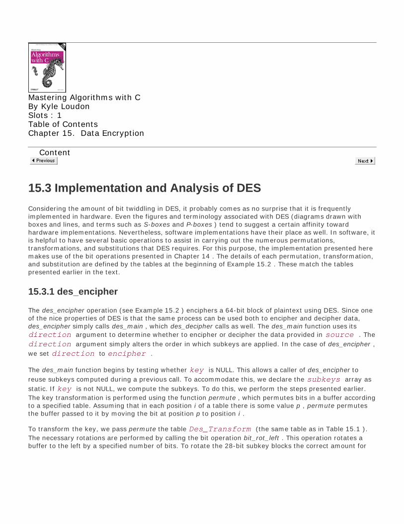
Mastering Algorithms with CBy Kyle LoudonSlots : 1Table of ContentsChapter 15. Data Encryption
Content
15.3 Implementation and Analysis of DES
Considering the amount of bit twiddling in DES, it probably comes as no surprise that it is frequentlyimplemented in hardware. Even the figures and terminology associated with DES (diagrams drawn withboxes and lines, and terms such as S-boxes and P-boxes ) tend to suggest a certain affinity towardhardware implementations. Nevertheless, software implementations have their place as well. In software, itis helpful to have several basic operations to assist in carrying out the numerous permutations,transformations, and substitutions that DES requires. For this purpose, the implementation presented heremakes use of the bit operations presented in Chapter 14 . The details of each permutation, transformation,and substitution are defined by the tables at the beginning of Example 15.2 . These match the tablespresented earlier in the text.
15.3.1 des_encipher
The des_encipher operation (see Example 15.2 ) enciphers a 64-bit block of plaintext using DES. Since oneof the nice properties of DES is that the same process can be used both to encipher and decipher data,des_encipher simply calls des_main , which des_decipher calls as well. The des_main function uses its
direction argument to determine whether to encipher or decipher the data provided in source . The
direction argument simply alters the order in which subkeys are applied. In the case of des_encipher ,
we set direction to encipher .
The des_main function begins by testing whether key is NULL. This allows a caller of des_encipher to
reuse subkeys computed during a previous call. To accommodate this, we declare the subkeys array as
static. If key is not NULL, we compute the subkeys. To do this, we perform the steps presented earlier.
The key transformation is performed using the function permute , which permutes bits in a buffer accordingto a specified table. Assuming that in each position i of a table there is some value p , permute permutesthe buffer passed to it by moving the bit at position p to position i .
To transform the key, we pass permute the table Des_Transform (the same table as in Table 15.1 ).
The necessary rotations are performed by calling the bit operation bit_rot_left . This operation rotates abuffer to the left by a specified number of bits. To rotate the 28-bit subkey blocks the correct amount for
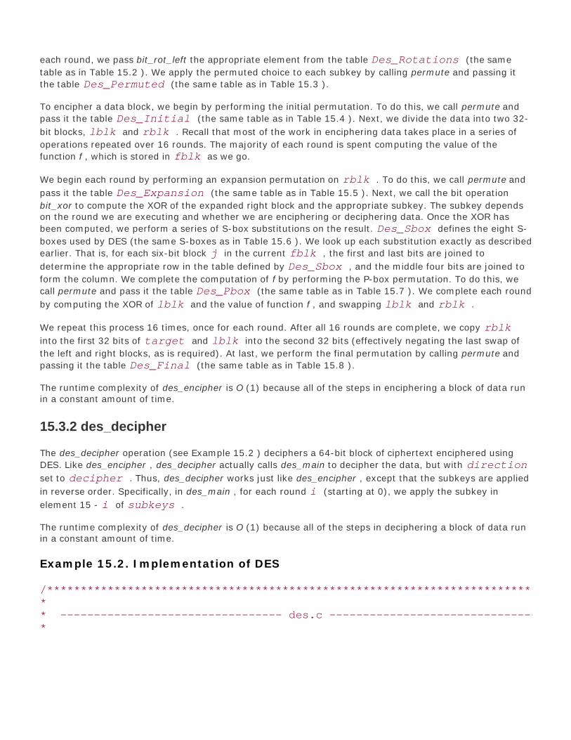
each round, we pass bit_rot_left the appropriate element from the table Des_Rotations (the same
table as in Table 15.2 ). We apply the permuted choice to each subkey by calling permute and passing it
the table Des_Permuted (the same table as in Table 15.3 ).
To encipher a data block, we begin by performing the initial permutation. To do this, we call permute and
pass it the table Des_Initial (the same table as in Table 15.4 ). Next, we divide the data into two 32-
bit blocks, lblk and rblk . Recall that most of the work in enciphering data takes place in a series of
operations repeated over 16 rounds. The majority of each round is spent computing the value of the
function f , which is stored in fblk as we go.
We begin each round by performing an expansion permutation on rblk . To do this, we call permute and
pass it the table Des_Expansion (the same table as in Table 15.5 ). Next, we call the bit operation
bit_xor to compute the XOR of the expanded right block and the appropriate subkey. The subkey dependson the round we are executing and whether we are enciphering or deciphering data. Once the XOR has
been computed, we perform a series of S-box substitutions on the result. Des_Sbox defines the eight S-
boxes used by DES (the same S-boxes as in Table 15.6 ). We look up each substitution exactly as described
earlier. That is, for each six-bit block j in the current fblk , the first and last bits are joined to
determine the appropriate row in the table defined by Des_Sbox , and the middle four bits are joined to
form the column. We complete the computation of f by performing the P-box permutation. To do this, we
call permute and pass it the table Des_Pbox (the same table as in Table 15.7 ). We complete each round
by computing the XOR of lblk and the value of function f , and swapping lblk and rblk .
We repeat this process 16 times, once for each round. After all 16 rounds are complete, we copy rblkinto the first 32 bits of target and lblk into the second 32 bits (effectively negating the last swap of
the left and right blocks, as is required). At last, we perform the final permutation by calling permute and
passing it the table Des_Final (the same table as in Table 15.8 ).
The runtime complexity of des_encipher is O (1) because all of the steps in enciphering a block of data runin a constant amount of time.
15.3.2 des_decipher
The des_decipher operation (see Example 15.2 ) deciphers a 64-bit block of ciphertext enciphered using
DES. Like des_encipher , des_decipher actually calls des_main to decipher the data, but with directionset to decipher . Thus, des_decipher works just like des_encipher , except that the subkeys are applied
in reverse order. Specifically, in des_main , for each round i (starting at 0), we apply the subkey in
element 15 - i of subkeys .
The runtime complexity of des_decipher is O (1) because all of the steps in deciphering a block of data runin a constant amount of time.
Example 15.2. Implementation of DES
/****************************************************************************** ** --------------------------------- des.c -------------------------------- ** *

*****************************************************************************/
#include <math.h>#include <stdlib.h>#include <string.h>
#include "bit.h"#include "encrypt.h"
/****************************************************************************** ** Define a mapping for the key transformation. ** ******************************************************************************/
static const int DesTransform[56] = {
57, 49, 41, 33, 25, 17, 9, 1, 58, 50, 42, 34, 26, 18, 10, 2, 59, 51, 43, 35, 27, 19, 11, 3, 60, 52, 44, 36, 63, 55, 47, 39, 31, 23, 15, 7, 62, 54, 46, 38, 30, 22, 14, 6, 61, 53, 45, 37, 29, 21, 13, 5, 28, 20, 12, 4
};
/****************************************************************************** ** Define the number of rotations for computing subkeys. ** ******************************************************************************/
static const int DesRotations[16] = {
1, 1, 2, 2, 2, 2, 2, 2, 1, 2, 2, 2, 2, 2, 2, 1
};
/****************************************************************************** ** Define a mapping for the permuted choice for subkeys. ** ******************************************************************************/
static const int DesPermuted[48] = {
14, 17, 11, 24, 1, 5, 3, 28, 15, 6, 21, 10, 23, 19, 12, 4, 26, 8, 16, 7, 27, 20, 13, 2,

41, 52, 31, 37, 47, 55, 30, 40, 51, 45, 33, 48, 44, 49, 39, 56, 34, 53, 46, 42, 50, 36, 29, 32
};
/****************************************************************************** ** Define a mapping for the initial permutation of data blocks. ** ******************************************************************************/
static const int DesInitial[64] = {
58, 50, 42, 34, 26, 18, 10, 2, 60, 52, 44, 36, 28, 20, 12, 4, 62, 54, 46, 38, 30, 22, 14, 6, 64, 56, 48, 40, 32, 24, 16, 8, 57, 49, 41, 33, 25, 17, 9, 1, 59, 51, 43, 35, 27, 19, 11, 3, 61, 53, 45, 37, 29, 21, 13, 5, 63, 55, 47, 39, 31, 23, 15, 7
};
/****************************************************************************** ** Define a mapping for the expansion permutation of data blocks. ** ******************************************************************************/
static const int DesExpansion[48] = {
32, 1, 2, 3, 4, 5, 4, 5, 6, 7, 8, 9, 8, 9, 10, 11, 12, 13, 12, 13, 14, 15, 16, 17, 16, 17, 18, 19, 20, 21, 20, 21, 22, 23, 24, 25, 24, 25, 26, 27, 28, 29, 28, 29, 30, 31, 32, 1
};
/****************************************************************************** ** Define tables for the S-box substitutions performed for data blocks. ** ******************************************************************************/
static const int DesSbox[8][4][16] = {
{ {14, 4, 13, 1, 2, 15, 11, 8, 3, 10, 6, 12, 5, 9, 0, 7}, { 0, 15, 7, 4, 14, 2, 13, 1, 10, 6, 12, 11, 9, 5, 3, 8},

{ 4, 1, 14, 8, 13, 6, 2, 11, 15, 12, 9, 7, 3, 10, 5, 0}, {15, 12, 8, 2, 4, 9, 1, 7, 5, 11, 3, 14, 10, 0, 6, 13}, },
{ {15, 1, 8, 14, 6, 11, 3, 4, 9, 7, 2, 13, 12, 0, 5, 10}, { 3, 13, 4, 7, 15, 2, 8, 14, 12, 0, 1, 10, 6, 9, 11, 5}, { 0, 14, 7, 11, 10, 4, 13, 1, 5, 8, 12, 6, 9, 3, 2, 15}, {13, 8, 10, 1, 3, 15, 4, 2, 11, 6, 7, 12, 0, 5, 14, 9}, },
{ {10, 0, 9, 14, 6, 3, 15, 5, 1, 13, 12, 7, 11, 4, 2, 8}, {13, 7, 0, 9, 3, 4, 6, 10, 2, 8, 5, 14, 12, 11, 15, 1}, {13, 6, 4, 9, 8, 15, 3, 0, 11, 1, 2, 12, 5, 10, 14, 7}, { 1, 10, 13, 0, 6, 9, 8, 7, 4, 15, 14, 3, 11, 5, 2, 12}, },
{ { 7, 13, 14, 3, 0, 6, 9, 10, 1, 2, 8, 5, 11, 12, 4, 15}, {13, 8, 11, 5, 6, 15, 0, 3, 4, 7, 2, 12, 1, 10, 14, 9}, {10, 6, 9, 0, 12, 11, 7, 13, 15, 1, 3, 14, 5, 2, 8, 4}, { 3, 15, 0, 6, 10, 1, 13, 8, 9, 4, 5, 11, 12, 7, 2, 14}, },
{ { 2, 12, 4, 1, 7, 10, 11, 6, 8, 5, 3, 15, 13, 0, 14, 9}, {14, 11, 2, 12, 4, 7, 13, 1, 5, 0, 15, 10, 3, 9, 8, 6}, { 4, 2, 1, 11, 10, 13, 7, 8, 15, 9, 12, 5, 6, 3, 0, 14}, {11, 8, 12, 7, 1, 14, 2, 13, 6, 15, 0, 9, 10, 4, 5, 3}, },
{ {12, 1, 10, 15, 9, 2, 6, 8, 0, 13, 3, 4, 14, 7, 5, 11}, {10, 15, 4, 2, 7, 12, 9, 5, 6, 1, 13, 14, 0, 11, 3, 8}, { 9, 14, 15, 5, 2, 8, 12, 3, 7, 0, 4, 10, 1, 13, 11, 6}, { 4, 3, 2, 12, 9, 5, 15, 10, 11, 14, 1, 7, 6, 0, 8, 13}, },
{ { 4, 11, 2, 14, 15, 0, 8, 13, 3, 12, 9, 7, 5, 10, 6, 1}, {13, 0, 11, 7, 4, 9, 1, 10, 14, 3, 5, 12, 2, 15, 8, 6}, { 1, 4, 11, 13, 12, 3, 7, 14, 10, 15, 6, 8, 0, 5, 9, 2}, { 6, 11, 13, 8, 1, 4, 10, 7, 9, 5, 0, 15, 14, 2, 3, 12}, },

{ {13, 2, 8, 4, 6, 15, 11, 1, 10, 9, 3, 14, 5, 0, 12, 7}, { 1, 15, 13, 8, 10, 3, 7, 4, 12, 5, 6, 11, 0, 14, 9, 2}, { 7, 11, 4, 1, 9, 12, 14, 2, 0, 6, 10, 13, 15, 3, 5, 8}, { 2, 1, 14, 7, 4, 10, 8, 13, 15, 12, 9, 0, 3, 5, 6, 11}, },
};
/****************************************************************************** ** Define a mapping for the P-box permutation of data blocks. ** ******************************************************************************/
static const int DesPbox[32] = {
16, 7, 20, 21, 29, 12, 28, 17, 1, 15, 23, 26, 5, 18, 31, 10, 2, 8, 24, 14, 32, 27, 3, 9, 19, 13, 30, 6, 22, 11, 4, 25
};
/****************************************************************************** ** Define a mapping for the final permutation of data blocks. ** ******************************************************************************/
static const int DesFinal[64] = {
40, 8, 48, 16, 56, 24, 64, 32, 39, 7, 47, 15, 55, 23, 63, 31, 38, 6, 46, 14, 54, 22, 62, 30, 37, 5, 45, 13, 53, 21, 61, 29, 36, 4, 44, 12, 52, 20, 60, 28, 35, 3, 43, 11, 51, 19, 59, 27, 34, 2, 42, 10, 50, 18, 58, 26, 33, 1, 41, 9, 49, 17, 57, 25
};
/****************************************************************************** ** Define a type for whether to encipher or decipher data. ** ******************************************************************************/
typedef enum DesEorD_ {encipher, decipher} DesEorD;
/*****************************************************************************
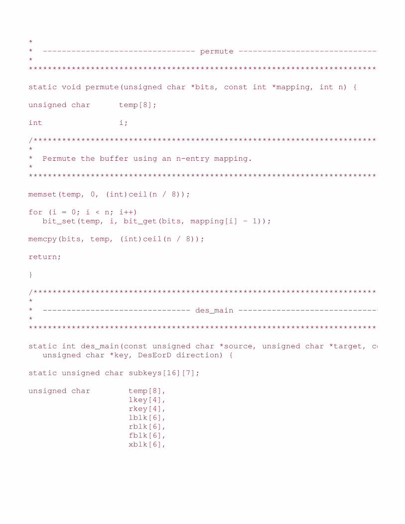
* ** -------------------------------- permute ------------------------------- ** ******************************************************************************/
static void permute(unsigned char *bits, const int *mapping, int n) {
unsigned char temp[8];
int i;
/****************************************************************************** ** Permute the buffer using an n-entry mapping. ** ******************************************************************************/
memset(temp, 0, (int)ceil(n / 8));
for (i = 0; i < n; i++) bit_set(temp, i, bit_get(bits, mapping[i] - 1));
memcpy(bits, temp, (int)ceil(n / 8));
return;
}
/****************************************************************************** ** ------------------------------- des_main ------------------------------- ** ******************************************************************************/
static int des_main(const unsigned char *source, unsigned char *target, const unsigned char *key, DesEorD direction) {
static unsigned char subkeys[16][7];
unsigned char temp[8], lkey[4], rkey[4], lblk[6], rblk[6], fblk[6], xblk[6],

sblk;
int row, col, i, j, k, p;
/****************************************************************************** ** If key is NULL, use the subkeys as computed in a previous call. ** ******************************************************************************/
if (key != NULL) {
/************************************************************************** * * * Make a local copy of the key. * * * **************************************************************************/
memcpy(temp, key, 8);
/************************************************************************** * * * Permute and compress the key into 56 bits. * * * **************************************************************************/
permute(temp, DesTransform, 56);
/************************************************************************** * * * Split the key into two 28-bit blocks. * * * **************************************************************************/
memset(lkey, 0, 4); memset(rkey, 0, 4);
for (j = 0; j < 28; j++) bit_set(lkey, j, bit_get(temp, j));
for (j = 0; j < 28; j++)

bit_set(rkey, j, bit_get(temp, j + 28));
/************************************************************************** * * * Compute the subkeys for each round. * * * **************************************************************************/
for (i = 0; i < 16; i++) {
/*********************************************************************** * * * Rotate each block according to its round. * * * ***********************************************************************/
bit_rot_left(lkey, 28, DesRotations[i]); bit_rot_left(rkey, 28, DesRotations[i]);
/*********************************************************************** * * * Concatenate the blocks into a single subkey. * * * ***********************************************************************/
for (j = 0; j < 28; j++) bit_set(subkeys[i], j, bit_get(lkey, j));
for (j = 0; j < 28; j++) bit_set(subkeys[i], j + 28, bit_get(rkey, j));
/*********************************************************************** * * * Do the permuted choice permutation. * * * ***********************************************************************/
permute(subkeys[i], DesPermuted, 48);
}
}
/****************************************************************************** ** Make a local copy of the source text. *

* ******************************************************************************/
memcpy(temp, source, 8);
/****************************************************************************** ** Do the initial permutation. ** ******************************************************************************/
permute(temp, DesInitial, 64);
/****************************************************************************** ** Split the source text into a left and right block of 32 bits. ** ******************************************************************************/
memcpy(lblk, &temp[0], 4);memcpy(rblk, &temp[4], 4);
/****************************************************************************** ** Encipher or decipher the source text. ** ******************************************************************************/
for (i = 0; i < 16; i++) {
/************************************************************************** * * * Begin the computation of f. * * * **************************************************************************/
memcpy(fblk, rblk, 4);
/************************************************************************** * * * Permute and expand the copy of the right block into 48 bits. * * * **************************************************************************/
permute(fblk, DesExpansion, 48);

/************************************************************************** * * * Apply the appropriate subkey for the round. * * * **************************************************************************/
if (direction == encipher) {
/*********************************************************************** * * * For enciphering, subkeys are applied in increasing order. * * * ***********************************************************************/
bit_xor(fblk, subkeys[i], xblk, 48); memcpy(fblk, xblk, 6);
}
else {
/*********************************************************************** * * * For deciphering, subkeys are applied in decreasing order. * * * ***********************************************************************/
bit_xor(fblk, subkeys[15 - i], xblk, 48); memcpy(fblk, xblk, 6);
}
/************************************************************************** * * * Do the S-box substitutions. * * * **************************************************************************/
p = 0;
for (j = 0; j < 8; j++) {
/*********************************************************************** * * * Compute a row and column into the S-box tables. * * *

***********************************************************************/
row = (bit_get(fblk, (j * 6)+0) * 2) + (bit_get(fblk, (j * 6)+5) * 1); col = (bit_get(fblk, (j * 6)+1) * 8) + (bit_get(fblk, (j * 6)+2) * 4) + (bit_get(fblk, (j * 6)+3) * 2) + (bit_get(fblk, (j * 6)+4) * 1);
/*********************************************************************** * * * Do the S-box substitution for the current six-bit block. * * * ***********************************************************************/
sblk = (unsigned char)DesSbox[j][row][col];
for (k = 4; k < 8; k++) {
bit_set(fblk, p, bit_get(&sblk, k)); p++;
}
}
/************************************************************************** * * * Do the P-box permutation to complete f. * * * **************************************************************************/
permute(fblk, DesPbox, 32);
/************************************************************************** * * * Compute the XOR of the left block and f. * * * **************************************************************************/
bit_xor(lblk, fblk, xblk, 32);
/************************************************************************** * * * Set the left block for the round. * * * **************************************************************************/
memcpy(lblk, rblk, 4);

/************************************************************************** * * * Set the right block for the round. * * * **************************************************************************/
memcpy(rblk, xblk, 4);
}
/****************************************************************************** ** Set the target text to the rejoined final right and left blocks. ** ******************************************************************************/
memcpy(&target[0], rblk, 4);memcpy(&target[4], lblk, 4);
/****************************************************************************** ** Do the final permutation. ** ******************************************************************************/
permute(target, DesFinal, 64);
return 0;
}
/****************************************************************************** ** ----------------------------- des_encipher ----------------------------- ** ******************************************************************************/
void des_encipher(const unsigned char *plaintext, unsigned char *ciphertext, const unsigned char *key) {
des_main(plaintext, ciphertext, key, encipher);
return;
}

/****************************************************************************** ** ----------------------------- des_decipher ----------------------------- ** ******************************************************************************/
void des_decipher(const unsigned char *ciphertext, unsigned char *plaintext, const unsigned char *key) {
des_main(ciphertext, plaintext, key, decipher);
return;
}
Top

Mastering Algorithms with CBy Kyle LoudonSlots : 1Table of ContentsChapter 15. Data Encryption
Content
15.4 DES Example: Block Cipher Modes
Most block ciphers, such as DES, encipher and decipher data in 64-bit blocks. Since nearly all of the workdone with ciphers involves more data than this, we end up invoking the cipher over and over again toprocess all of the blocks. The specific manner in which a block cipher is invoked repeatedly is called a blockcipher mode .
The simplest way to process several blocks of data is to append each block of ciphertext we generate toothers generated before it. This primitive approach is called ECB , or electronic code book . Its simplicitymakes it very popular, but it is relatively insecure. Its main problem is that for any given key, a specificblock of plaintext always enciphers to the same block of ciphertext wherever it appears in the data. Thismeans that if an adversary cracks even a small section of the data, he can begin to develop a code book forcracking other sections as well. A better approach is CBC , or cipher block chaining .
CBC mode avoids the problems of ECB by augmenting a block cipher with simple operations and feedback .Feedback makes each block of ciphertext depend in some way on actions performed earlier. In CBC mode,previous blocks of ciphertext serve as feedback so that even the same block of plaintext is likely to encipherinto a different block of ciphertext each time it appears.
For previous blocks of ciphertext to serve as feedback, before we encipher a block of plaintext, we XOR itwith the block of ciphertext generated before it. When we decipher the ciphertext, we XOR each decipheredblock back with the block of ciphertext it follows. Simply stated:
where Ci and Pi are the i th blocks of ciphertext and plaintext from buffers C and P , and EK and DK are theencipher and decipher operations using key K .
Usually we add one random block of data to the beginning of the plaintext. This is so that even when anadversary has some idea what the first block of plaintext contains, it cannot be used to start replicating thechaining sequence. This block is called the initialization vector . We encipher it normally, without anyfeedback, then use it as the feedback when enciphering and deciphering the first real block of plaintext.

Example 15.3 presents an implementation of two functions, cbc_encipher and cbc_decipher , that encipherand decipher a buffer of data using DES in CBC mode. The cbc_encipher function takes a buffer of plaintext
containing size bytes and enciphers it using key as the key. It assumes that the first block of plaintext
is actually the 64-bit initialization vector. The cbc_decipher function takes a buffer of ciphertext containing
size bytes and deciphers it using key as the key. For symmetry, the initialization vector is deciphered
as well and is returned as the first block of plaintext.
The runtime complexities of cbc_encipher and cbc_decipher are both O (n ), where n is the number ofblocks enciphered or deciphered. This is because the two functions simply call the O (1) operationsdes_encipher and des_decipher , respectively, once for each block.
Example 15.3. Implementation of Functions for DES in CBC Mode
/****************************************************************************** ** --------------------------------- cbc.c -------------------------------- ** ******************************************************************************/
#include <stdlib.h>
#include "bit.h"#include "cbc.h"#include "encrypt.h"
/****************************************************************************** ** ----------------------------- cbc_encipher ----------------------------- ** ******************************************************************************/
void cbc_encipher(const unsigned char *plaintext, unsigned char *ciphertext, const unsigned char *key, int size) {
unsigned char temp[8];
int i;
/****************************************************************************** ** Encipher the initialization vector. ** ******************************************************************************/
des_encipher(&plaintext[0], &ciphertext[0], key);

/****************************************************************************** ** Encipher the buffer using DES in CBC mode. ** ******************************************************************************/
i = 8;
while (i < size) {
bit_xor(&plaintext[i], &ciphertext[i - 8], temp, 64); des_encipher(temp, &ciphertext[i], NULL); i = i + 8;
}
return;
}
/****************************************************************************** ** ----------------------------- cbc_decipher ----------------------------- ** ******************************************************************************/
void cbc_decipher(const unsigned char *ciphertext, unsigned char *plaintext, const unsigned char *key, int size) {
unsigned char temp[8];
int i;
/****************************************************************************** ** Decipher the initialization vector. ** ******************************************************************************/
des_decipher(&ciphertext[0], &plaintext[0], key);
/****************************************************************************** ** Decipher the buffer using DES in CBC mode. ** ******************************************************************************/

i = 8;
while (i < size) {
des_decipher(&ciphertext[i], temp, NULL); bit_xor(&ciphertext[i - 8], temp, &plaintext[i], 64); i = i + 8;
}
return;
}
Top

Mastering Algorithms with CBy Kyle Loudon
Slots : 1
Table of Contents
Chapter 15. Data Encryption
Content
15.5 Description of RSA
RSA (Rivest-Shamir-Adleman) is one of the most popular asymmetric, or public-key, ciphers. RSA isasymmetric because the key used to encipher data is not the same key used to decipher it. Like DES,RSA is a block cipher, but the block size varies depending on the size of the keys. If the amount ofdata to be encrypted is not an even multiple of this size, it is padded in some application-specificway.
One important implication of RSA being an asymmetric cipher is that when transmitting data across anetwork, the key used to encipher the data does not have to be transmitted with the data itself.Thus, there is less chance of having the key compromised. RSA is also useful when partiesenciphering data are not allowed to decipher the data of others. Parties who wish to encipher datause one key, which is considered public, while parties allowed to decipher the data use a second key,which they keep private.
RSA is considered very secure, but it runs considerably slower than DES. As with DES, the security ofRSA has never been proven, but it is related to the difficult problem of factoring large numbers(numbers containing at least 200 decimal digits). Since no efficient solutions are known for thisproblem, it is conjectured that there are no efficient ways to crack RSA.
RSA is based on principles that are less obtuse than the numerous permutations and substitutionsperformed in DES. Fundamentally, enciphering and deciphering data revolves around modularexponentiation, an operation in modular arithmetic. Modular arithmetic is integer arithmetic as usualexcept that when we work modulo n, every result x is replaced with a member of {0, 1, . . . , n - 1}so that x mod n is the remainder of x /n. For example, 40 mod 11 = 7 because 40/11 = 3 with aremainder of 7. Modular exponentiation is the process of computing ab mod n.
15.5.1 Computing Public and Private Keys
In RSA, the public key and private key work together as a pair. The public key is used to encipher ablock of data, after which only the corresponding private key can be used to decipher it. Whengenerating keys, we follow a few steps to ensure that this marriage works. These steps also ensurethat there is no practical way to determine one key from the other.
To begin, we select two large prime numbers, which are called p and q (see the related topics at theend of the chapter). Considering today's factoring technology, these each should be at least 200

decimal digits to be considered secure in practice. We then compute n, the product of thesenumbers:
n = pq
Next, we choose a small odd integer e, which will become part of the public key. The most importantconsideration in choosing e is that it should have no factors in common with (p - 1)(q - 1). In otherwords, e is relatively prime with (p - 1) (q - 1). For example, if p = 11 and q = 19, then n = (11)(19)= 209. Here we might choose e = 17 because (p - 1)(q - 1) = (10)(18) = 180, and 17 and 180 haveno common factors. Common choices for e are 3, 17, and 65,537. Using one of these values does notjeopardize the security of RSA because deciphering data is a function of the private key.
Once we have chosen a value for e, we compute a corresponding value d, which will become part ofthe private key. To do this, we compute the multiplicative inverse of e, modulo (p - 1)(q - 1), asfollows:
d = e-1 mod (p-1)(q-1)
The way to think of this is: what value of d satisfies ed mod (p - 1)(q - 1) = 1? For example, in theequation 17d mod 180 = 1, one possible value for d is 53. Other possibilities are 233, 413, 593, andso forth. An extension of Euclid's algorithm is used to compute multiplicative modular inverses inpractice (see the related topics at the end of the chapter). In this book, code is provided for using dand e but not for deriving them.
Now that we have values for both e and d, we publish (e, n) as the public key P and keep (d, n)secret as the private key S, as shown:
p = (e, n)
S = (d,n)
Parties who encipher data use P. Those who decipher data use S. To ensure that even someone whoknows P cannot compute S, the values used for p and q must never be revealed.
The security offered by P and S together comes from the fact that multiplication is a good one-wayfunction. One-way functions are fundamental to cryptography. Simply stated, a one-way function is afunction that is relatively easy to compute in one direction but impractical to reverse. For example, inRSA, multiplying p and q is a one-way function because although multiplying p and q is easy,factoring n back into p and q is extremely time-consuming, provided the values chosen for p and qare large enough.
The steps performed to compute P and S have their origin in some interesting properties of Euler'sfunction (pronounced "oiler"). In particular, these properties allow us to do useful things withmodular exponentiation. Euler's function, denoted f (n), defines how many numbers less than n arerelatively prime with n. Two numbers are said to be relatively prime if their only common factor is 1.As an example of Euler's function, f (8) = 4 because there are four numbers less than 8 that arerelatively prime with 8, namely 1, 3, 5, and 7.
Euler's function has two properties that are particularly relevant to RSA. First, when n is prime, f (n)= n - 1. This is because the only factors of n are 1 and n; thus, n is relatively prime with all of the n -1 numbers before it. Another interesting property is that f (n) is the exponential period modulo n fornumbers relatively prime with n. This means that for any number a < n relatively prime with n, a f(n) mod n = 1. For example, 14 mod 8 = 1, 34 mod 8 = 1, 54 mod 8 = 1, and 74 mod 8 = 1.

Multiplying both sides of this equation by a yields:
Hence, 15 mod 8 = 1, 35 mod 8 = 3, 55 mod 8 = 5, and 75 mod 8 = 7. This algebraic adjustment ispowerful because for some equation c = me mod n, it lets us find a value d so that c d mod n = m.This is the identity that allows us to encipher data in RSA and then decipher the data back as shownbelow:
The relationship of Euler's function with exponential periods guarantees that any block of data weencipher will decipher again uniquely. To find d, we solve the equation d = e - 1f (n) + 1.Unfortunately, there is not always an integer solution to d = e - 1f (n) + 1. For example, consider if e= 5 and n = 13. In this case, d = (1/5)((13 - 1) + 1) = (1/5)(13). To deal with this, we compute dmodulo f (n). In other words, d = (e - 1f (n) + 1) mod f (n), which can be simplified to:
We can make this simplification because (f (n) + 1) mod f (n) = (f (n) + 1) - f (n) = 1. We canverify this by inserting any number in place of f (n). Notice the similarity between this equation andthe one used for d earlier in the steps for computing keys. This provides a way to compute d from eand n. Of course, since e and n are public and potentially known to an adversary, one might ask:doesn't this give an adversary the same opportunity to compute the private key? At this point it isworth examining where RSA's security comes from.
RSA gets its security from the critical fact that Euler's function is multiplicative. This means that if pand q are relatively prime (which they are if we choose them both to be prime), then f (pq) = f (p)f(q). Thus, if we have two primes p and q, and n = pq, then f (n) = (p - 1)(q - 1), and mostimportantly:
d = e-1 mod (p-1)(q-1)
Therefore, even though an adversary might know both e and n, in order to compute d, she wouldhave to know f (n), which can only be determined in a practical manner by knowing both p and q.Since these are not known, the adversary is left to factor n, an extremely time-consuming process,provided the values chosen for p and q are large enough.
15.5.2 Enciphering and Deciphering Data Blocks
To encipher and decipher data with RSA, we first need to choose a block size. To do this, we mustensure that the largest value that the block can store, considering its total number of bits, is lessthan n. For example, if p and q are primes containing 200 decimal digits, n will be just under 400decimal digits. Therefore, we should choose a block size small enough to store only those numberswith less than this many decimal digits. In practice, we often choose the block size in bits to be thelargest power of 2 less than n. For example, if n were 209, we would choose a block size of 7 bitsbecause 27 = 128 is less than 209, but 28 = 256 is greater.
To encipher a block of plaintext Mi, the i th block of data from a buffer M, we use the public key (e,

n) to take the numerical value of Mi, raise it to the power of e, and take the result modulo n. Thisyields a block of ciphertext Ci. The modulo n operation ensures that Ci will fit into the same size blockas the plaintext. Thus, to encipher a block of plaintext:
It was mentioned earlier that Euler's function is the basis for using modular exponentiation toencipher data using this equation and, in the equation that follows, for being able to get the originalplaintext back. To decipher a block of ciphertext Ci, the i th block of ciphertext from a buffer C, weuse the private key (d, n) to take the numeric value of Ci , raise it to the power of d, and take theresult modulo n. This yields the original block of plaintext Mi. Thus, to decipher a block of ciphertext:
Top

Mastering Algorithms with CBy Kyle Loudon
Slots : 1
Table of Contents
Chapter 15. Data Encryption
Content
15.6 Interface for RSA
rsa_encipher
void rsa_encipher(Huge plaintext, Huge *ciphertext, RsaPubKey pubkey);
Return Value
None.
Description
Uses RSA to encipher one block of plaintext specified by plaintext. Specify the public key (e, n) inthe RsaPubKey structure pubkey. A block the same size as plaintext is returned inciphertext. It is the responsibility of the caller to manage the storage required in ciphertext. Toencipher a large buffer of data, call rsa_encipher in accordance with a block cipher mode (see theexample earlier in this chapter).
Complexity
O (1)
rsa_decipher
void rsa_decipher(Huge ciphertext, Huge *plaintext, RsaPriKey prikey);
Return Value
None.

Description
Uses RSA to decipher one block of ciphertext specified by ciphertext. Specify the private key (d, n)in the RsaPriKey structure prikey. A block the same size as ciphertext is returned inplaintext. It is the responsibility of the caller to manage the storage required in plaintext. Todecipher a large buffer of data, call rsa_decipher in accordance with the block cipher mode used todecipher the data.
Complexity
O (1)
Top

Mastering Algorithms with CBy Kyle LoudonSlots : 1Table of ContentsChapter 15. Data Encryption
Content
15.7 Implementation and Analysis of RSA
Because encryption with RSA requires little more than computing ab mod n , a basic implementation isrelatively simple: all we need is a function to perform modular exponentiation. However, to make RSAsecure, recall that we must use large integers. This complicates things. Specifically, all arithmetic must beperformed with integers that are twice the size of the keys. (We will see in a moment that this doubling isrequired for the modular exponentiation process.) Thus, if the keys are 200 decimal digits, we need anabstract datatype that supports integers with at least 400 decimal digits.
Since support for large-integer arithmetic is not provided in this book, the RSA implementation presentedhere must depend on another library. Several are available. Instead of providing this support, the datatype
Huge has been defined (see Example 15.1 ). In a secure implementation we can typedef this to a large-
integer abstract datatype of our choice. The only other requirement is that we replace each operator in
expressions containing Huge integers with operations defined for the type. For purposes of illustration in
the implementation presented here, Huge is made a typedef to an unsigned long integer, an intrinsic type
that usually offers 10 decimal digits. This means that the implementation as it exists in Example 15.4supports keys up to only 5 decimal digits. Thus, the implementation is functional, but it would not be
considered secure without redefining Huge to a larger type.
15.7.1 rsa_encipher
The rsa_encipher operation (see Example 15.4 ) enciphers a block of plaintext using RSA. It does this bycalling the function modexp , which computes ab mod n , where a is the block of plaintext, and b and n aremembers e and n of the public key. For efficiency, modexp uses a method called binary square and multiplyto perform modular exponentiation .
The binary square and multiply method avoids the huge intermediate result produced by ab when a and bare both large. For example, imagine computing ab mod n when a , b , and n are all integers containing200 decimal digits. The result is a 40,000-digit integer modulo a 200-digit integer! Since this eventuallyyields an integer of 200 decimal digits, the goal is to avoid the 40,000-digit intermediate result.
The binary square and multiply method computes ab mod n primarily as the product of several squares

(see Figure 15.4 ). We start with the binary representation of b and process bits from the right. For each bitin b , we square a , take the result modulo n , and store this value back into a . Each time we encounter abit in b that is 1, we multiply the current value of a times another register y (initially 1) and store the resultback into y . Once we reach the most significant bit in b , y contains the value of ab mod n . Throughoutthe process, the largest value ever computed is a 2 . Therefore, if a is an integer containing 200 decimaldigits, we never have to deal with integers larger than 400 digits, which is a considerable improvement overthe 40,000-digit number mentioned a moment ago. The shaded areas of Figure 15.4 illustrate this processfor 511 mod 53 = 48,828,125 mod 53 = 20. In this calculation, the largest value we end up handling is 422
= 1764, as opposed to 511 = 48,828,125.
The runtime complexity of rsa_encipher is O (1) because all of the steps in enciphering a block of data runin a constant amount of time. Since the block size is constant, the loop in modexp runs in a constantamount of time.
Figure 15.4. Modular exponentiation using the binary square and multiplymethod
15.7.2 rsa_decipher
The rsa_decipher operation (see Example 15.4 ) deciphers a block of ciphertext enciphered using RSA. Itdoes this by calling the function modexp , which computes ab mod n , where a is the block of ciphertext,and b and n are members d and n of the private key. This proceeds in the same manner as described forrsa_encipher .
The runtime complexity of rsa_decipher is O (1) because all of the steps in deciphering a block of data runin a constant amount of time. Since the block size is constant, the loop in modexp runs in a constantamount of time.
Example 15.4. Implementation of RSA
/****************************************************************************** ** --------------------------------- rsa.c -------------------------------- ** ******************************************************************************/

#include "encrypt.h"
/****************************************************************************** ** -------------------------------- modexp -------------------------------- ** ******************************************************************************/
static Huge modexp(Huge a, Huge b, Huge n) {
Huge y;
/****************************************************************************** ** Compute pow(a, b) % n using the binary square and multiply method. ** ******************************************************************************/
y = 1;
while (b != 0) {
/************************************************************************** * * * For each 1 in b, accumulate y. * * * **************************************************************************/
if (b & 1) y = (y * a) % n;
/************************************************************************** * * * Square a for each bit in b. * * * **************************************************************************/
a = (a * a) % n;
/************************************************************************** * * * Prepare for the next bit in b. * * * **************************************************************************/
b = b >> 1;

}
return y;
}
/****************************************************************************** ** ----------------------------- rsa_encipher ----------------------------- ** ******************************************************************************/
void rsa_encipher(Huge plaintext, Huge *ciphertext, RsaPubKey pubkey) {
*ciphertext = modexp(plaintext, pubkey.e, pubkey.n);
return;
}
/****************************************************************************** ** ----------------------------- rsa_decipher ----------------------------- ** ******************************************************************************/
void rsa_decipher(Huge ciphertext, Huge *plaintext, RsaPriKey prikey) {
*plaintext = modexp(ciphertext, prikey.d, prikey.n);
return;
}
Top

Mastering Algorithms with CBy Kyle Loudon
Slots : 1
Table of Contents
Chapter 15. Data Encryption
Content
15.8 Questions and Answers
Q: Suppose we would like to encrypt a file containing flags that enable or disable certain attributes inan application based on the features a customer has paid for. Which method of encryption presentedin this chapter would be best suited to this scenario?
A: Since in this scenario only one party, the application itself, needs to read the file, it makes senseto use a symmetric cipher such as DES. Before installing the file, we encipher it with a key that onlythe application knows about. Whenever the application needs to read the file, it deciphers it using thesame key.
Q: Suppose a party A is making sensitive requests for data across the Internet to another party B. Bis the only one who should be able to decipher the data enciphered by A, and A is the only one whoshould be able to decipher data enciphered by B specifically for A. B also receives requests fromseveral other parties, all of whom should not be able to hear what each other is saying. Whichmethod of encryption from this chapter would be best in this scenario?
A: Since all parties must be able to communicate with B but without anyone else being able todecipher the communications, we should use a public-key cipher such as RSA. Consider the case of Amaking a request to B. A makes his request to B by enciphering the request with B 's public key.When B receives the request, B deciphers it using her own private key. Once B has validated that Asent the request (perhaps using a digital signature), she enciphers a reply using A's public key. OnceA receives the reply from B, A deciphers the message using his own private key.
Q: With DES, we encipher and decipher data by performing a series of permutations andsubstitutions. Exactly how these permutations and substitutions affect the data is essentially afunction of 16 subkeys, derived from an initial key that we provide. In general, the security of DES isgreatest when most of the subkeys differ from one another. Unfortunately, certain initial keys lead tosituations in which all subkeys are identical. These initial keys are called weak keys. DES has fourweak keys. What are they?
A: To generate subkeys in DES, we first transform the key from 64 bits to 56 bits. Once the key hasbeen transformed, we divide it into two 28-bit blocks and perform a number of other operations thatare repeated during each round. If either of the two 28-bit blocks contains bits that are all the same,these operations have no effect. Thus, we end up with subkeys that are identical for every round,and the initial key is considered weak. The four weak keys of DES and what they become are shownin Table 15.9.

Table 15.9. Weak Keys in DES Before and After the Key Transformation
Key Becomes
0101 0101 0101 0101 0000000 0000000
1F1F 1F1F 1F1F 1F1F 0000000 FFFFFFF
E0E0 E0E0 F1F1 F1F1 FFFFFFF 0000000
FEFE FEFE FEFE FEFE FFFFFFF FFFFFFF
Q: Avoiding weak keys is one security issue in DES. Another issue is avoiding semiweak keys.Semiweak keys come in pairs. Two keys form a semiweak key pair if the subkeys they produce are inthe opposite order. This means that if we use one key from the pair to re-encipher the ciphertextgenerated using the other key, we effectively get the same result as deciphering the ciphertext withthe original key. DES has six semiweak key pairs. What are they? Why are semiweak keys aproblem?
A: The problem with semiweak key pairs in DES is that by re-enciphering the ciphertext with one keyin the pair we essentially end up performing the same operation as deciphering the ciphertext withthe other key. Thus, effectively we have two keys that can decipher the data, which makes semiweakkeys undesirable. The six semiweak key pairs of DES are shown in Table 15.10.
Table 15.10. Semiweak Key Pairs in DES
Key 1 Key 2
01FE 01FE 01FE 01FE FE01 FE01 FE01 FE01
1FE0 1FE0 0EF1 0EF1 E01F E01F F10E F10E
01E0 01E0 01F1 01F1 E001 E001 F101 F101
1EFE 1EFE 0EFE 0EFE FE1F FE1F FE0E FE0E
011F 011F 010E 010E 1F01 1F01 0E01 0E01
E0FE E0FE F1FE F1FE FEE0 FEE0 FEF1 FEF1
Q: Some applications of DES use keys that are generated randomly. In applications like this, whatprecautions might we take against the use of weak and semiweak keys, if any?
A: Considering the number of keys listed in Tables Table 15.9 and Table 15.10 combined, it's evidentthat out of 256 possible keys in DES, weak and semiweak keys are rare. Nevertheless, applicationsthat use randomly generated keys often check to make sure a candidate key is not weak orsemiweak before using it. On the other hand, since checking every key is somewhat wastefulconsidering how infrequent weak and semiweak keys are, many applications simply don't worryabout them.

Q: RSA is a block cipher, which means that it processes data one block at a time. Whereas DESalways uses a block size of 64 bits, the block size of RSA varies depending on the value of n, where n= pq. What happens if we mistakenly choose the block size so that some blocks of plaintext containvalues greater than or equal to n?
A: The problem with a block of plaintext containing a value greater than or equal to n is that whenwe encipher and decipher blocks, the modular exponentiation operation is modulo n. This means thatall blocks generated as either ciphertext or plaintext contain values less than n. Therefore, if theoriginal block of plaintext contains a value greater than or equal to n, after enciphering anddeciphering the block, we will not end up with the plaintext we started with.
Q: This chapter discussed two common block cipher modes, ECB and CBC. What are some of theadvantages each offers? What are some of the drawbacks?
A: ECB and CBC both have advantages and disadvantages. ECB is simple, but its lack of feedbackmakes it considerably less secure than CBC. However, by not using feedback, ECB has someflexibilities. For example, with ECB, since no block depends on any other block having been processedbefore it, we can process blocks out of sequence or in parallel. The most significant advantage of CBCis that it conceals patterns in the plaintext well. However, its use of feedback means that we mustencipher blocks in order. On the other hand, deciphering data in CBC mode does not have thisrestriction. To decipher data, we require feedback only from the ciphertext itself, not any of theblocks deciphered previously.
Top

Mastering Algorithms with CBy Kyle Loudon
Slots : 1
Table of Contents
Chapter 15. Data Encryption
Content
15.9 Related Topics
Finding large prime numbers
An essential part of computing secure keys for RSA. One of the best methods for doing this isthe Miller-Rabin algorithm, which also makes use of Euclid's algorithm. Miller-Rabin isprobabilistic, so on rare occasions it may yield a number that is in fact composite (in fact, thisis extremely rare, but nevertheless possible). For this reason, primes generated in this fashionare sometimes called industrial-grade primes.
Modular arithmetic
A type of arithmetic particularly useful in encryption as well as other areas of computerscience. Modular arithmetic is integer arithmetic as usual except that when we are workingmodulo n, every result x is replaced with a member of {0, 1, . . . , n - 1} so that x mod n is theremainder of x/n.
Arithmetic with large integers
An essential part of secure implementations of RSA. In RSA, to be secure considering currentfactoring technology, we must choose keys that have at least 200 decimal digits. This meansthat all integer arithmetic must be performed with integers of at least 400 digits.
Euclid's greatest common divisor algorithm
A method of computing greatest common divisors, and one of the oldest known algorithms.The algorithm is particularly relevant to RSA because we can extend it to help computemultiplicative modular inverses.
CFB (cipher feedback) and OFB (output feedback)
Common block cipher modes in addition to the ECB and CBC modes presented in this chapter.CFB uses ciphertext for feedback in such a way that a block cipher appears more like a streamcipher. Stream ciphers process data in continuous streams instead of one block at a time. Thiscan be useful in network applications, where data often arrives in bursts that are not alignedwith the block size. OFB is another method of running a block cipher as a stream cipher, butthe feedback is independent of both the plaintext and ciphertext.
Cryptographic protocols
Step-by-step procedures executed by two or more parties in order to communicate with eachother in a secure manner. It is important to realize that many problems in data security requiremore than just simply enciphering and deciphering data. Often we need to establish secure

protocols, of which ciphers are only a part.
Top

Mastering Algorithms with CBy Kyle LoudonSlots : 1Table of ContentsPart III: Algorithms
Content
Chapter 16. Graph AlgorithmsGraphs are flexible data structures that model problems defined in terms of relationships or connectionsbetween objects (see Chapter 11 ). This chapter presents algorithms that work with graphs. As we will see,many graph algorithms resemble the fundamental ones for breadth-first and depth-first search introducedin Chapter 11 . Breadth-first and depth-first search are important to many other graph algorithms becausethey offer good ways of exploring the structure of a graph in a systematic manner.
One significant difference between the algorithms of Chapter 11 and the ones in this chapter, however, isthat the algorithms here work with weighted graphs . In a weighted graph , each edge is assigned a value,or weight , which is represented pictorially as a small number beside the edge. Although weights can meanmany things, in general they represent a cost associated with traversing an edge. Weighted graphs andtheir algorithms have an enormous capacity to model real problems. Example 16.1 is a header for thegraph algorithms presented in this chapter.
This chapter covers:
Minimum spanning trees
Trees that serve as abstractions of many connectivity problems. A minimum spanning tree is a treethat connects all vertices in an undirected, weighted graph at a minimum cost.
Shortest paths
The result of solving various types of shortest-path problems. A shortest path is a path that connectsone vertex to another in a directed, weighted graph at a minimum cost.
Traveling-salesman problem
A surprisingly difficult problem in which we look for the shortest tour that visits every vertex in acomplete, undirected, weighted graph exactly once before returning to the first vertex.
Some applications of graph algorithms are :
Efficient pipelines

A practical concern in transporting water, oil, and other liquids. If distribution points for the pipelineare represented as vertices in a graph, and candidate connections between the points as edges areweighted by the cost to connect the points, a minimum spanning tree gives us the best way to lay apipeline that connects all of the distribution points.
Routing tables (illustrated in this chapter)
Tables used by routers to help direct data through an internet. The purpose of a router is to movedata closer to its final destination. In one type of routing, routers periodically compute shortest pathsto one another so each knows the best next step for sending data to certain destinations.
Delivery services
Services that typically visit numerous locations to pick up and deliver packages. Solving the traveling-salesman problem can indicate the most efficient way for a vehicle operated by a service to visitevery location exactly once before returning to its starting point.
Communication networks
Networks containing many different types of equipment including telephone lines, relay stations, andsatellite systems, all of which must be located in an optimal manner. An optimal arrangement can bedetermined by computing a minimum spanning tree for the weighted graph that models the network.
Routing airplanes
An optimization problem particularly important to airlines and air traffic control agencies. Oftenairplanes cannot fly directly from one point to another. Instead, they weave their way through airwaystructures, or highways in the sky, considering winds, monetary charges for traversing airspace, andair traffic control restrictions. The best route between two points is the path with the minimum weightdefined in terms of factors like these.
Closed transport systems
Systems in which railroad cars or conveyor carts repeatedly tour several points. Systems like thesemight be used to deliver parts in a factory or to move inventory in and out of a warehouse. Solvingthe traveling-salesman problem can indicate the best way to construct the system.
Wiring circuit boards
An optimization problem in electronics manufacturing. Often it is necessary to make the pins ofseveral components on a circuit board electrically equivalent by establishing a connection betweenthem. If each pin is represented as a vertex in a graph, and candidate connections as edges weightedby the amount of wire required for the connection, a minimum spanning tree gives us the best way toconnect the pins.
Traffic monitoring
The process of watching changes in traffic flow to determine the best route between two points in acity. To avoid excessive traffic delays, we can use a weighted graph to model the flow of traffic alongroadways and look for the path from intersection to intersection with the minimum traffic.
Example 16.1. Header for Graph Algorithms
/****************************************************************************** ** ------------------------------ graphalg.h ------------------------------ ** ******************************************************************************/

#ifndef GRAPHALG_H#define GRAPHALG_H
#include "graph.h"#include "list.h"
/****************************************************************************** ** Define a structure for vertices in minimum spanning trees. ** ******************************************************************************/
typedef struct MstVertex_ {
void *data;double weight;
VertexColor color;double key;
struct MstVertex_ *parent;
} MstVertex;
/****************************************************************************** ** Define a structure for vertices in shortest-path problems. ** ******************************************************************************/
typedef struct PathVertex_ {
void *data;double weight;
VertexColor color;double d;
struct PathVertex_ *parent;
} PathVertex;
/****************************************************************************** ** Define a structure for vertices in traveling-salesman problems. ** *

*****************************************************************************/
typedef struct TspVertex_ {
void *data;
double x, y;
VertexColor color;
} TspVertex;
/****************************************************************************** ** --------------------------- Public Interface --------------------------- ** ******************************************************************************/
int mst(Graph *graph, const MstVertex *start, List *span, int (*match)(const void *key1, const void *key2));
int shortest(Graph *graph, const PathVertex *start, List *paths, int (*match) (const void *key1, const void *key2));
int tsp(List *vertices, const TspVertex *start, List *tour, int (*match) (const void *key1, const void *key2));
#endif
Top

Mastering Algorithms with CBy Kyle Loudon
Slots : 1
Table of Contents
Chapter 16. Graph Algorithms
Content
16.1 Description of Minimum Spanning Trees
Picture a number of pegs on a board connected by pieces of string. Assuming that every peg isreachable from any other by traveling along one or more strings, imagine a game in which the objectis to remove some of the strings until all of the pegs remain connected using the least amount ofstring. This is the idea behind a minimum spanning tree. Formally stated, given an undirected,weighted graph G = (V, E ), a minimum spanning tree is the set T of edges in E that connect allvertices in V at a minimum cost. The edges in T form a tree because each vertex ends up withexactly one parent that precedes it in the span, with the exception of the first vertex, which is theroot of the tree.
16.1.1 Prim's Algorithm
One approach to computing a minimum spanning tree is Prim's algorithm. Prim's algorithm grows aminimum spanning tree by adding edges one at a time based on which looks best at the moment.The fact that Prim's algorithm adds edges using this approach makes it greedy (see Chapter 1).Although greedy algorithms often yield approximations rather than optimal solutions, Prim'salgorithm actually provides an optimal result.
Fundamentally, the algorithm works by repeatedly selecting a vertex and exploring the edgesincident on it to determine if there is a more effective way to span the vertices explored thus far. Thealgorithm resembles breadth-first search because it explores all edges incident on a vertex beforemoving deeper in the graph. To determine the vertex to select at each stage, we maintain a colorand a key value with every vertex.
Initially, we set all colors to white and we set all key values to , which represents an arbitrarilylarge value greater than the weight of any edge in the graph. We set the key value of the vertex atwhich to start the span to 0. As the algorithm progresses, we assign to all vertices except the startvertex a parent in the minimum spanning tree. A vertex is part of the minimum spanning tree onlyafter it is colored black. Before this time, its parent can fluctuate.
Prim's algorithm proceeds as follows. First, from among all white vertices in the graph, we select thevertex u with the smallest key value. Initially, this will be the start vertex since its key value is 0.After we select the vertex, we color it black. Next, for each white vertex v adjacent to u, if the weightof the edge (u, v) is less than the key value of v, we set the key value of v to the weight of (u, v)and we set the parent of v to u. We then repeat this process until all vertices have been colored

black. As the minimum spanning tree grows, it consists of all edges in the graph that have a blackvertex on either end.
Figure 16.1 illustrates the computation of a minimum spanning tree using Prim's algorithm. In thefigure, the key value and parent of each vertex are displayed beside the vertex. The key value is tothe left of the slash, and the parent is to the right. The edges shaded in light gray are the edges inthe minimum spanning tree as it grows. The minimum spanning tree computed in the figure has atotal weight of 17.
Figure 16.1. Computing a minimum spanning tree using Prim's algorithm
Top

Mastering Algorithms with CBy Kyle Loudon
Slots : 1
Table of Contents
Chapter 16. Graph Algorithms
Content
16.2 Interface for Minimum Spanning Trees
mst
int mst(Graph *graph, const MstVertex *start, List *span, int (*match) (const void *key1, const void *key2));
Return Value
0if computing the minimum spanning tree is successful, or -1 otherwise.
Description
Computes a minimum spanning tree for an undirected, weighted graph specified by graph. The minimumspanning tree is computed starting from the vertex specified by start. The operation modifies graph,so a copy should be made before calling the operation, if necessary. Each vertex in graph must containdata of type MstVertex. Assign a weight to each edge by setting the weight member of theMstVertex structure passed as data2 to graph_ins_edge. Use the data member of eachMstVertex structure to store data associated with the vertex, such as an identifier. The match functionfor graph, which is set by the caller when initializing the graph with graph_init, should compare only thedata members of MstVertex structures. This is the same function that should be passed as thematch argument to mst. Once computed, information about the minimum spanning tree is returned inspan, which is a list of MstVertex structures. In span, the vertex whose parent is set to NULL is thevertex at the root of the minimum spanning tree. The parent member of every other vertex points tothe vertex that precedes it in the span. The vertices in span point to actual vertices in graph, so thecaller must ensure that the storage in graph remains valid as long as span is being accessed. Uselist_destroy to destroy span once it is no longer needed.
Complexity
O (EV 2), where V is the number of vertices in the graph and E is the number of edges. However, with alittle improvement to the implementation presented here, Prim's algorithm runs in O (E lg V ) time (see

the related topics at the end of the chapter).
Top

Mastering Algorithms with CBy Kyle LoudonSlots : 1Table of ContentsChapter 16. Graph Algorithms
Content
16.3 Implementation and Analysis of Minimum SpanningTrees
To compute a minimum spanning tree for an undirected, weighted graph, we first need a way to representweighted graphs using the basic abstract datatype for graphs presented in Chapter 11 . We also need away to keep track of the information that Prim's algorithm requires for vertices and edges. This is the point
of the MstVertex structure; it is used for vertices in graphs for which we plan to compute minimum
spanning trees (see Example 16.2 ). The structure consists of five members: data is the data associated
with the vertex, weight is the weight of the edge incident to the vertex, color is the color of the
vertex, key is the key value of the vertex, and parent is the parent of the vertex in the minimum
spanning tree.
Building a graph of MstVertex structures is nearly the same as building a graph containing other types
of data. To insert a vertex into the graph, we call graph_ins_vertex and pass an MstVertex structure for
data . Similarly, to insert an edge, we call graph_ins_edge and pass MstVertex structures for data1and data2 . When we insert a vertex, we set only the data member of the MstVertex structure.
When we insert an edge, we set the data member of data1 , and the data and weight members
of data2 . In data2 , the weight member is the weight of the edge from the vertex represented by
data1 to the vertex represented by data2 . In practice, weights are usually computed and stored as
floating-point numbers. Since key values are computed from the weights, these are floating-point numbersas well.
The mst operation begins by initializing every vertex in the list of adjacency-list structures. We set the
initial key value of each vertex to DBL_MAX , except the start vertex, whose key value is set to 0.0. Recall
that in the graph abstract datatype, a graph was represented as a list of adjacency-list structures, each ofwhich contained one vertex and a set of vertices adjacent to it (see Chapter 11 ). We use the vertex storedin each adjacency-list structure to maintain the color, key value, and parent of the vertex. The point ofmaintaining this information in the list of adjacency-list structures, as opposed to vertices in the adjacencylists themselves, is that we can keep it in one place. Whereas a single vertex may appear in numerousadjacency lists, each vertex appears in the list of adjacency-list structures exactly once.

At the center of Prim's algorithm is a single loop that iterates once for each vertex in the graph. We begineach iteration by selecting the vertex that has the smallest key value among the white vertices. We colorthis vertex black where it resides in the list of adjacency-list structures. Next, we traverse the verticesadjacent to the selected vertex. As we traverse each vertex, we look up its color and key value in the list ofadjacency-list structures. Once we have located this information, we compare it with the color and keyvalue of the selected vertex. If the adjacent vertex is white and its key value is less than that of theselected vertex, we set the key value of the adjacent vertex to the weight of the edge between the selectedvertex and the adjacent vertex; we also set the parent of the adjacent vertex to the selected vertex. Weupdate this information for the adjacent vertex where it resides in the list of adjacency-list structures. Wethen repeat this process until all vertices have been colored black.
Once the main loop in Prim's algorithm terminates, we are finished computing the minimum spanning tree.
At this point, we insert each black MstVertex structure from the list of adjacency-list structures into the
linked list span . In span , the vertex whose parent is set to NULL is the vertex at the root of the
minimum spanning tree. The parent member of every other vertex points to the vertex that precedes it
in the span. The weight member of each MstVertex structure is not populated because it is needed
only for storing weights in adjacency lists. Figure 16.2 shows the list of MstVertex structures returned
for the minimum spanning tree computed in Figure 16.1 .
Figure 16.2. The list returned by mst for the minimum spanning treecomputed in Figure 16.1
The runtime complexity of mst is O (EV 2 ), where V is the number of vertices in the graph and E is thenumber of edges. This comes from the main loop, in which we select vertices and compare weights and keyvalues. For each of the V vertices we select, we first traverse V elements in the list of adjacency-liststructures to determine which white vertex has the smallest key value. This part of the main loop is O (V 2 )overall. Next, for each vertex adjacent to the vertex we select, we consult the list of adjacency-liststructures for information about whether to change its key value and parent. Over all V vertices, the list isconsulted E times, once for each of the E edges in all of the adjacency lists together. Each of theseconsultations requires O (V ) time to search the list. Therefore, for all V vertices that we select, an O (V )operation is performed E times. Consequently, this part of the loop is O (EV 2 ), and the main loop overall isO (V 2 + EV 2 ), or O (EV 2 ). Since the loops before and after the main loop are O (V ), the runtimecomplexity of mst is O (EV 2 ). However, recall that with a little improvement (discussed at the end of thechapter), Prim's algorithm runs in O (E lg V ) time.
Example 16.2. Implementation for Computing Minimum Spanning Trees
/****************************************************************************** ** --------------------------------- mst.c -------------------------------- *

* ******************************************************************************/
#include <float.h>#include <stdlib.h>
#include "graph.h"#include "graphalg.h"#include "list.h"
/****************************************************************************** ** ---------------------------------- mst --------------------------------- ** ******************************************************************************/
int mst(Graph *graph, const MstVertex *start, List *span, int (*match)(const void *key1, const void *key2)) {
AdjList *adjlist;
MstVertex *mst_vertex, *adj_vertex;
ListElmt *element, *member;
double minimum;
int found, i;
/****************************************************************************** ** Initialize all of the vertices in the graph. ** ******************************************************************************/
found = 0;
for (element = list_head(&graph_adjlists(graph)); element != NULL; element = list_next(element)) {
mst_vertex = ((AdjList *)list_data(element))->vertex;
if (match(mst_vertex, start)) {

/*********************************************************************** * * * Initialize the start vertex. * * * ***********************************************************************/
mst_vertex->color = white; mst_vertex->key = 0; mst_vertex->parent = NULL; found = 1;
}
else {
/*********************************************************************** * * * Initialize vertices other than the start vertex. * * * ***********************************************************************/
mst_vertex->color = white; mst_vertex->key = DBL_MAX; mst_vertex->parent = NULL;
}
}
/****************************************************************************** ** Return if the start vertex was not found. ** ******************************************************************************/
if (!found) return -1;
/****************************************************************************** ** Use Prim's algorithm to compute a minimum spanning tree. ** ******************************************************************************/
i = 0;

while (i < graph_vcount(graph)) {
/************************************************************************** * * * Select the white vertex with the smallest key value. * * * **************************************************************************/
minimum = DBL_MAX;
for (element = list_head(&graph_adjlists(graph)); element != NULL; element = list_next(element)) {
mst_vertex = ((AdjList *)list_data(element))->vertex;
if (mst_vertex->color == white && mst_vertex->key < minimum) {
minimum = mst_vertex->key; adjlist = list_data(element);
}
}
/************************************************************************** * * * Color the selected vertex black. * * * **************************************************************************/
((MstVertex *)adjlist->vertex)->color = black;
/************************************************************************** * * * Traverse each vertex adjacent to the selected vertex. * * * **************************************************************************/
for (member = list_head(&adjlist->adjacent); member != NULL; member = list_next(member)) {
adj_vertex = list_data(member);
/*********************************************************************** * * * Find the adjacent vertex in the list of adjacency-list structures. *

* * ***********************************************************************/
for (element = list_head(&graph_adjlists(graph)); element != NULL; element = list_next(element)) {
mst_vertex = ((AdjList *)list_data(element))->vertex;
if (match(mst_vertex, adj_vertex)) {
/***************************************************************** * * * Decide whether to change the key value and parent of the * * adjacent vertex in the list of adjacency-list structures. * * * *****************************************************************/
if (mst_vertex->color == white && adj_vertex->weight < mst_vertex->key) {
mst_vertex->key = adj_vertex->weight; mst_vertex->parent = adjlist->vertex;
}
break;
}
}
}
/************************************************************************** * * * Prepare to select the next vertex. * * * **************************************************************************/
i++;
}
/****************************************************************************** ** Load the minimum spanning tree into a list. *

* ******************************************************************************/
list_init(span, NULL);
for (element = list_head(&graph_adjlists(graph)); element != NULL; element = list_next(element)) {
/************************************************************************** * * * Load each black vertex from the list of adjacency-list structures. * * * **************************************************************************/
mst_vertex = ((AdjList *)list_data(element))->vertex;
if (mst_vertex->color == black) {
if (list_ins_next(span, list_tail(span), mst_vertex) != 0) {
list_destroy(span); return -1;
}
}
}
return 0;
}
Top

Mastering Algorithms with CBy Kyle Loudon
Slots : 1
Table of Contents
Chapter 16. Graph Algorithms
Content
16.4 Description of Shortest Paths
Finding the shortest path, or minimum-weight path, from one vertex to another in a graph is animportant distillation of many routing problems. Formally stated, given a directed, weighted graph G= (V, E ), the shortest path from vertex s to t in V is the set S of edges in E that connect s to t at aminimum cost.
When we find S, we are solving the single-pair shortest-path problem. To do this, in actuality wesolve the more general single-source shortest-paths problem , which solves the single-pair shortest-path problem in the process. In the single-source shortest-paths problem, we compute the shortestpaths from a start vertex s to all other vertices reachable from it. We solve this problem because noalgorithm is known to solve the single-pair shortest-path problem any faster.
16.4.1 Dijkstra's Algorithm
One approach to solving the single-source shortest-paths problem is Dijkstra's algorithm(pronounced "Dikestra"). Dijkstra's algorithm grows a shortest-paths tree, whose root is the startvertex s and whose branches are the shortest paths from s to all other vertices in G. The algorithmrequires that all weights in the graph be nonnegative. Like Prim's algorithm, Dijkstra's algorithm isanother example of a greedy algorithm that happens to produce an optimal result. The algorithm isgreedy because it adds edges to the shortest-paths tree based on which looks best at the moment.
Fundamentally, Dijkstra's algorithm works by repeatedly selecting a vertex and exploring the edgesincident from it to determine whether the shortest path to each vertex can be improved. Thealgorithm resembles a breadth-first search because it explores all edges incident from a vertexbefore moving deeper in the graph. To compute the shortest paths between s and all other vertices,Dijkstra's algorithm requires that a color and shortest-path estimate be maintained with everyvertex. Typically, shortest-path estimates are represented by the variable d.
Initially, we set all colors to white, and we set all shortest-path estimates to , which represents anarbitrarily large value greater than the weight of any edge in the graph. We set the shortest-pathestimate of the start vertex to 0. As the algorithm progresses, we assign to all vertices except thestart vertex a parent in the shortest-paths tree. The parent of a vertex may change several timesbefore the algorithm terminates.
Dijkstra's algorithm proceeds as follows. First, from among all white vertices in the graph, we select

the vertex u with the smallest shortest-path estimate. Initially, this will be the start vertex since itsshortest-path estimate is 0. After we select the vertex, we color it black. Next, for each white vertexv adjacent to u, we relax the edge (u, v). When we relax an edge, we determine whether goingthrough u improves the shortest path computed thus far to v. To make this decision, we add theweight of (u, v) to the shortest-path estimate for u. If this value is less than or equal to the shortest-path estimate for v, we assign the value to v as its new shortest-path estimate, and we set theparent of v to u. We then repeat this process until all vertices have been colored black. Once we havecomputed the shortest-paths tree, the shortest path from s to another vertex t can be determined bystarting at t in the tree and following successive parents until we reach s. The path in reverse is theshortest path from s to t.
Figure 16.3 illustrates the computation of the shortest paths between a and all other vertices in thegraph. The shortest path from a to b, for example, is <a, c, f, b>, which has a total weight of 7. Theshortest-path estimate and parent of each vertex are displayed beside the vertex. The shortest-pathestimate is to the left of the slash, and the parent is to the right. The edges shaded in light gray arethe edges in the shortest-paths tree as it changes.
Figure 16.3. Computing shortest paths using Dijkstra's algorithm

Top
Mastering Algorithms with CBy Kyle LoudonSlots : 1Table of ContentsChapter 16. Graph Algorithms
Content
16.5 Interface for Shortest Pathsshortest
int shortest(Graph *graph, const PathVertex *start, List *paths, int (*match) (const void *key1, const void *key2));
Return Value
0 if computing the shortest paths is successful, or -1 otherwise.
Description
Computes shortest paths between start and all other vertices in a directed, weighted graph specified by
graph . The operation modifies graph , so a copy should be made before calling the operation, if
necessary. Each vertex in graph must contain data of type PathVertex . Assign a weight to each
edge by setting the weight member of the PathVertex structure passed as data2 to
graph_ins_edge . Use the data member of each PathVertex structure to store data associated with
the vertex, such as an identifier. The match function for graph , which is set by the caller when
initializing the graph with graph_init , should compare only the data members of PathVertexstructures. This is the same function that should be passed as the match argument to shortest . Once
computed, information about the shortest paths is returned in paths , which is a list of PathVertexstructures. In paths , the parent of the start vertex is set to NULL. The parent member of every other
vertex points to the vertex that precedes it in the shortest path from the start vertex. The vertices in
paths point to actual vertices in graph , so the caller must ensure that the storage in graph remains
valid as long as paths is being accessed. Use list_destroy to destroy paths once it is no longer needed.
Complexity

O (EV 2 ), where V is the number of vertices in the graph and E is the number of edges. However, with alittle improvement (similar to that discussed for Prim's algorithm at the end of the chapter), Dijkstra'salgorithm can run in O (E lg V ) time.
Top

Mastering Algorithms with CBy Kyle LoudonSlots : 1Table of ContentsChapter 16. Graph Algorithms
Content
16.6 Implementation and Analysis of Shortest Paths
To compute the shortest paths from a vertex to all others reachable from it in a directed, weighted graph,the graph is represented in the same manner as described for minimum spanning trees. However, we use
the PathVertex structure instead of MstVertex for vertices (see Example 16.3 ). The PathVertexstructure allows us to represent weighted graphs as well as keep track of the information that Dijkstra's
algorithm requires for vertices and edges. The structure consists of five members: data is the data
associated with the vertex, weight is the weight of the edge incident to the vertex, color is the color
of the vertex, d is the shortest-path estimate for the vertex, and parent is the parent of the vertex in
the shortest-paths tree. We build a graph consisting of PathVertex structures in the same manner as
described for building graphs with MstVertex structures.
The shortest operation begins by initializing every vertex in the list of adjacency-list structures. We set the
initial shortest-path estimate for each vertex to DBL_MAX , except the start vertex, whose estimate is set
to 0.0. The vertex stored in each adjacency-list structure is used to maintain the color, shortest-pathestimate, and parent of the vertex, for the same reasons as mentioned for computing minimum spanningtrees.
At the center of Dijkstra's algorithm is a single loop that iterates once for each vertex in the graph. Webegin each iteration by selecting the vertex that has the smallest shortest-path estimate among the whitevertices. We color this vertex black where it resides in the list of adjacency-list structures. Next, wetraverse the vertices adjacent to the selected vertex. As we traverse each vertex, we look up its color andshortest-path estimate in the list of adjacency-list structures. Once we have located this information, wecall relax to relax the edge between the selected vertex and the adjacent vertex. If relax needs to updatethe shortest-path estimate and parent of the adjacent vertex, it does so where the adjacent vertex residesin the list of adjacency-list structures. We then repeat this process until all vertices have been coloredblack.
Once the main loop in Dijkstra's algorithm terminates, we are finished computing the shortest paths fromthe start vertex to all other vertices reachable from it in the graph. At this point, we insert each black
PathVertex structure from the list of adjacency-list structures into the linked list paths . In paths ,
the parent of the start vertex is set to NULL. The parent member of every other vertex points to the

vertex that precedes it in the shortest path from the start vertex. The weight member of each
PathVertex structure is not populated because it is needed only for storing weights in adjacency lists.
Figure 16.4 shows the list of PathVertex structures returned for the shortest paths computed in Figure
16.3 .
Figure 16.4. The list returned by the operation shortest for the shortest pathscomputed in Figure 16.3
The runtime complexity of shortest is O (EV 2 ), where V is the number of vertices in the graph and E is thenumber of edges. This comes from the main loop, in which we select vertices and relax edges. For each ofthe V vertices we select, we first traverse V elements in the list of adjacency-list structures to determinewhich white vertex has the smallest shortest-path estimate. This part of the main loop is O (V 2 ) overall.Next, for each vertex adjacent to the vertex we select, the list of adjacency-list structures is consulted forthe information needed to relax the edge between the two vertices. Over all V vertices that we select, thelist is consulted E times, once for each of the E edges in all of the adjacency lists together. Each of theseconsultations requires O (V ) time to search the list. Therefore, for all V vertices that we select, an O (V )operation is performed E times. Consequently, this part of the loop is O (EV 2 ), and the main loop overall isO (V 2 + EV 2 ), or O (EV 2 ). Since the loops before and after the main loop are O (V ), the runtimecomplexity of shortest is O (EV 2 ). However, recall that with a little improvement (similar to that discussedfor Prim's algorithm at the end of the chapter), Dijkstra's algorithm can run in O (E lg V ) time.
Example 16.3. Implementation for Computing Shortest Paths
/***************************************************************************** ** ----------------------------- shortest.c ------------------------------ ** *****************************************************************************/
#include <float.h>#include <stdlib.h>
#include "graph.h"#include "graphalg.h"#include "list.h"#include "set.h"
/****************************************************************************** *
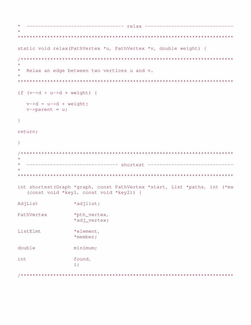
* --------------------------------- relax -------------------------------- ** ******************************************************************************/
static void relax(PathVertex *u, PathVertex *v, double weight) {
/****************************************************************************** ** Relax an edge between two vertices u and v. ** ******************************************************************************/
if (v->d > u->d + weight) {
v->d = u->d + weight; v->parent = u;
}
return;
}
/****************************************************************************** ** ------------------------------- shortest ------------------------------- ** ******************************************************************************/
int shortest(Graph *graph, const PathVertex *start, List *paths, int (*match) (const void *key1, const void *key2)) {
AdjList *adjlist;
PathVertex *pth_vertex, *adj_vertex;
ListElmt *element, *member;
double minimum;
int found, i;
/*****************************************************************************

* ** Initialize all of the vertices in the graph. ** ******************************************************************************/
found = 0;
for (element = list_head(&graph_adjlists(graph)); element != NULL; element = list_next(element)) {
pth_vertex = ((AdjList *)list_data(element))->vertex;
if (match(pth_vertex, start)) {
/*********************************************************************** * * * Initialize the start vertex. * * * ***********************************************************************/
pth_vertex->color = white; pth_vertex->d = 0; pth_vertex->parent = NULL; found = 1;
}
else {
/*********************************************************************** * * * Initialize vertices other than the start vertex. * * * ***********************************************************************/
pth_vertex->color = white; pth_vertex->d = DBL_MAX; pth_vertex->parent = NULL;
}
}
/****************************************************************************** ** Return if the start vertex was not found. *

* ******************************************************************************/
if (!found) return -1;
/****************************************************************************** ** Use Dijkstra's algorithm to compute shortest paths from the start vertex. ** ******************************************************************************/
i = 0;
while (i < graph_vcount(graph)) {
/************************************************************************** * * * Select the white vertex with the smallest shortest-path estimate. * * * **************************************************************************/
minimum = DBL_MAX;
for (element = list_head(&graph_adjlists(graph)); element != NULL; element = list_next(element)) {
pth_vertex = ((AdjList *)list_data(element))->vertex;
if (pth_vertex->color == white && pth_vertex->d < minimum) {
minimum = pth_vertex->d; adjlist = list_data(element);
}
}
/************************************************************************** * * * Color the selected vertex black. * * * **************************************************************************/
((PathVertex *)adjlist->vertex)->color = black;

/************************************************************************** * * * Traverse each vertex adjacent to the selected vertex. * * * **************************************************************************/
for (member = list_head(&adjlist->adjacent); member != NULL; member = list_next(member)) {
adj_vertex = list_data(member);
/*********************************************************************** * * * Find the adjacent vertex in the list of adjacency-list structures. * * * ***********************************************************************/
for (element = list_head(&graph_adjlists(graph)); element != NULL; element = list_next(element)) {
pth_vertex = ((AdjList *)list_data(element))->vertex;
if (match(pth_vertex, adj_vertex)) {
/***************************************************************** * * * Relax the adjacent vertex in the list of adjacency-list * * structures. * * * *****************************************************************/
relax(adjlist->vertex, pth_vertex, adj_vertex->weight);
}
}
}
/************************************************************************** * * * Prepare to select the next vertex. * * * **************************************************************************/
i++;

}
/****************************************************************************** ** Load the vertices with their path information into a list. ** ******************************************************************************/
list_init(paths, NULL);
for (element = list_head(&graph_adjlists(graph)); element != NULL; element = list_next(element)) {
/************************************************************************** * * * Load each black vertex from the list of adjacency-list structures. * * * **************************************************************************/
pth_vertex = ((AdjList *)list_data(element))->vertex;
if (pth_vertex->color == black) {
if (list_ins_next(paths, list_tail(paths), pth_vertex) != 0) {
list_destroy(paths); return -1;
}
}
}
return 0;
}
Top
Mastering Algorithms with CBy Kyle LoudonSlots : 1Table of ContentsChapter 16. Graph Algorithms
Content
16.7 Shortest Paths Example: Routing Tables
One application in which shortest paths play an important role is routing data between networks in aninternet. Routing is the process of making informed decisions about how to move data from one point toanother. In an internet, this is accomplished by propagating small sections of the data, or packets , alonginterconnected points called gateways . As each packet passes through a gateway, a router looks at wherethe packet eventually needs to go and decides to which gateway it should be sent next. The goal of eachrouter is to propagate a packet closer and closer to its final destination.
In order to propagate a packet closer to its destination, each router maintains information about thestructure, or topology , of the internet. It stores this information in a routing table . A routing table containsone entry for each gateway the router knows how to reach. Each entry specifies the next gateway to whichpackets destined for another gateway should be sent.
So that packets are continually sent along the best route possible, routers periodically update their routingtables to reflect changes in the internet. In one type of routing, called shortest path first routing , or SPFrouting , every router maintains its own map of the internet so that it can update its routing table bycomputing shortest paths between itself and other destinations. Its map is a directed, weighted graphwhose vertices are gateways and whose edges are connections between the gateways. Each edge isweighted by the performance most recently observed for a connection. From time to time, routersexchange information about topology and performance using a protocol designed especially for thispurpose.
Example 16.4 is a function, route, that computes the information necessary to update one entry in a
routing table using SPF routing. The function accepts the list of path information returned in the pathsargument of shortest . It uses this information to determine to which gateway a router should send apacket next to reach its destination most effectively.
To complete an entire table for a specific gateway, we first call shortest with the gateway passed as start. Next, for each destination to be included in the routing table, we call route with the destination passed as
destination . We pass the same function for match as was provided to graph_init for the graph
from which paths was generated. The route function follows parent pointers in paths from the
destination back to the gateway and returns the best choice for moving a packet closer to its destination in

next . The vertex returned in next points to the actual vertex in paths , so the storage in pathsmust remain valid as long as next is being accessed.
Figure 16.5 a illustrates the computation of a routing table for a router at gw1 i n the internet shown(modeled using a graph similar to the one in Figure 16.3 ). Figure 16.5 b illustrates the computation of therouting table for a router at gw2 . Notice how the shortest paths are different depending on where we startin the internet. Also, notice that in Figure 16.5 b there is no way to reach gw1 , so there is no entry for it inthe table.
Figure 16.5. Routing tables computed for gateways (a) gw1 and (b) gw2 , inan internet
The runtime complexity of route is O (n 2 ), where n is the number of gateways in paths . This is because
we look up in paths the parent of each vertex between the destination we are interested in and the
starting point in the internet. If the shortest path between us and the destination contains every gateway in
paths , in the worst case we may have to search the list of gateways n times to find every parent.
Example 16.4. Implementation of a Function for Updating Entries in RoutingTables
/****************************************************************************** ** -------------------------------- route.c ------------------------------- ** ******************************************************************************/
#include <stdlib.h>
#include "graphalg.h"#include "list.h"#include "route.h"
/*****************************************************************************

* ** --------------------------------- route -------------------------------- ** ******************************************************************************/
int route(List *paths, PathVertex *destination, PathVertex **next, int (*match)(const void *key1, const void *key2)) {
PathVertex *temp, *parent;
ListElmt *element;
int found;
/****************************************************************************** ** Locate the destination in the list of gateways. ** ******************************************************************************/
found = 0;
for (element = list_head(paths); element != NULL; element = list_next(element)) {
if (match(list_data(element), destination)) {
temp = list_data(element); parent = ((PathVertex *)list_data(element))->parent; found = 1; break;
}
}
/****************************************************************************** ** Return if the destination is not reachable. ** ******************************************************************************/
if (!found) return -1;

/****************************************************************************** ** Compute the next gateway in the shortest path to the destination. ** ******************************************************************************/
while (parent != NULL) {
temp = list_data(element); found = 0;
for (element = list_head(paths); element != NULL; element = list_next(element)) {
if (match(list_data(element), parent)) {
parent = ((PathVertex *)list_data(element))->parent; found = 1; break;
}
}
/************************************************************************** * * * Return if the destination is not reachable. * * * **************************************************************************/
if (!found) return -1;
}
*next = temp;
return 0;
}
Top

Mastering Algorithms with CBy Kyle Loudon
Slots : 1
Table of Contents
Chapter 16. Graph Algorithms
Content
16.8 Description of the Traveling-Salesman Problem
Imagine a salesman who needs to visit a number of cities as part of the route he works. His goal is totravel the shortest possible distance while visiting every city exactly once before returning to thepoint at which he starts. This is the idea behind the traveling-salesman problem.
In a graph, a tour in which we visit every other vertex exactly once before returning to the vertex atwhich we started is called a hamiltonian cycle. To solve the traveling-salesman problem, we use agraph G = (V, E ) as a model and look for the hamiltonian cycle with the shortest length. G is acomplete, undirected, weighted graph, wherein V is a set of vertices representing the points we wishto visit and E is a set of edges representing connections between the points. Each edge in E isweighted by the distance between the vertices that define it. Since G is complete and undirected, Econtains V (V - 1)/2 edges.
One way to solve the traveling-salesman problem is by exploring all possible permutations of thevertices in G. Using this approach, since each permutation represents one possible tour, we simplydetermine which one results in the tour that is the shortest. Unfortunately, this approach is not at allpractical because it does not run in polynomial time. A polynomial-time algorithm is one whosecomplexity is less than or equal to O (nk), where k is some constant. This approach does not run inpolynomial time because for a set of V vertices, there are V ! possible permutations; thus, exploringthem all requires O (V !) time, where V ! is the factorial of V, which is the product of all numbersfrom V down to 1.
In general, nonpolynomial-time algorithms are avoided because even for small inputs, problemsquickly become intractable. Actually, the traveling-salesman problem is a special type ofnonpolynomial-time problem called NP-complete. NP-complete problems are those for which nopolynomial-time algorithms are known, but for which no proof refutes the possibility either; even so,the likelihood of finding such an algorithm is extremely slim. With this in mind, normally thetraveling-salesman problem is solved using an approximation algorithm (see Chapter 1).
16.8.1 Applying the Nearest-Neighbor Heuristic
One way to compute an approximate traveling-salesman tour is to apply the nearest-neighborheuristic. This works as follows. We begin with a tour consisting of only the vertex at the start of thetour. We color this vertex black. All other vertices are white until added to the tour, at which point wecolor them black as well. Next, for each vertex v not already in the tour, we compute a weight for the

edge between the last vertex u added to the tour and v. Recall that the weight of an edge from u to vin the traveling-salesman problem is the distance between u and v. We compute this using thecoordinates of the points that each vertex represents. The distance r between two points (x1, y1) and(x2, y2) is defined by the formula:
Using this formula, we select the vertex closest to u, color it black, and add it to the tour. We thenrepeat this process until all vertices have been colored black. At this point, we add the start vertex tothe tour again to form a complete cycle.
Figure 16.6 illustrates a solution to the traveling-salesman problem using the nearest-neighborheuristic. Normally when a graph is drawn for the traveling-salesman problem, the edges connectingevery vertex to each other are not explicitly shown since the edges are understood. In the figure,each vertex is displayed along with the coordinates of the point it represents. The dashed lines ateach stage show the edges whose distances are being compared. The darkest line is the edge addedto the tour. The tour obtained using the nearest-neighbor heuristic has a length of 15.95. Theoptimal tour has a length of 14.71, which is about 8% shorter.
Figure 16.6. Solving the traveling-salesman problem using the nearest-neighbor heuristic

The nearest-neighbor heuristic has some interesting properties. Like the other algorithms in thischapter, it resembles breadth-first search because it explores all of the vertices adjacent to the lastvertex in the tour before exploring deeper in the graph. The heuristic is also greedy because eachtime it adds a vertex to the tour, it does so based on which looks best at the moment. Unfortunately,the nearest neighbor added at one point may affect the tour in a negative way later. Nevertheless,the heuristic always returns a tour whose length is within a factor of 2 of the optimal tour length, andin many cases it does better than this. Other techniques exist to improve a tour once we havecomputed it. One technique is to apply an exchange heuristic (see the related topics at the end of thechapter).
Top

Mastering Algorithms with CBy Kyle LoudonSlots : 1Table of ContentsChapter 16. Graph Algorithms
Content
16.9 Interface for the Traveling-Salesman Problemtsp
int tsp(List *vertices, const TspVertex *start, List *tour, int (*match) (const void *key1, const void *key2))
Return Value
0if computing the approximate traveling-salesman tour is successful, or -1 otherwise.
Description
Computes an approximate traveling-salesman tour of the points specified as vertices in vertices . The
tour begins at the vertex specified by start . The operation modifies vertices , so a copy should be
made before calling the operation, if necessary. Each element in vertices must be of type TspVertex. Use the data member of each TspVertex structure to store data associated with the vertex, such as
an identifier. Use the x and y members of the structure to specify the coordinates associated with the
vertex. The function specified by match determines whether two vertices match. It should only compare
the data members of TspVertex structures. The tour is returned in tour , which is a list of
TspVertex structures. Each vertex appears in tour in the order it would be encountered during the
tour. The elements in tour point to the actual vertices in vertices , so the caller must ensure that the
storage in vertices remains valid as long as tour is being accessed. Use list_destroy to destroy
tour once it is no longer needed.
Complexity
O (V 2 ), where V is the number of vertices to visit in the tour.

Top

Mastering Algorithms with CBy Kyle LoudonSlots : 1Table of ContentsChapter 16. Graph Algorithms
Content
16.10 Implementation and Analysis of the Traveling-SalesmanProblem
To solve the traveling-salesman problem, we begin with a graph that is represented simply as a list ofvertices. In this representation, an edge connecting every pair of vertices is implied. Each vertex in the list
is a TspVertex structure (see Example 16.5 ). This structure consists of four members: data is the
data associated with the vertex, x and y are coordinates for the point the vertex represents, and coloris the color of the vertex.
The tsp operation begins by coloring every vertex white, except the start vertex, which is colored black andadded to the tour immediately. The coordinates of the start vertex are also recorded so that we cancompute distances between it and every other vertex during the first iteration of the main loop. In the mainloop, we add all of the remaining vertices to the tour. During each iteration, we look for the white vertexclosest to the last vertex. Each time we add a vertex, we record its coordinates for the next iteration andcolor the vertex black. After the loop terminates, we add the start vertex again to complete the tour.
The runtime complexity of tsp is O (V 2 ), where V is the number of vertices to visit in the tour. This isbecause for each of the V - 1 iterations of the main loop, we search the vertices in the graph to determinewhich is white and needs a distance computed to it. Notice that O (V 2 ) is quite an improvement over theruntime complexity for computing an optimal tour, which was O (V !).
Example 16.5. Implementation for Solving the Traveling-Salesman Problem
/****************************************************************************** ** --------------------------------- tsp.c -------------------------------- ** ******************************************************************************/
#include <float.h>
#include <math.h>#include <stdlib.h>
#include "graph.h"#include "graphalg.h"#include "list.h"
/****************************************************************************** ** ---------------------------------- tsp --------------------------------- ** ******************************************************************************/
int tsp(List *vertices, const TspVertex *start, List *tour, int (*match) (const void *key1, const void *key2)) {
TspVertex *tsp_vertex, *tsp_start, *selection;
ListElmt *element;
double minimum, distance, x, y;
int found, i;
/****************************************************************************** ** Initialize the list for the tour. ** ******************************************************************************/
list_init(tour, NULL);
/****************************************************************************** ** Initialize all of the vertices in the graph. ** ******************************************************************************/
found = 0;

for (element = list_head(vertices); element != NULL; element = list_next(element)) {
tsp_vertex = list_data(element);
if (match(tsp_vertex, start)) {
/*********************************************************************** * * * Start the tour at the start vertex. * * * ***********************************************************************/
if (list_ins_next(tour, list_tail(tour), tsp_vertex) != 0) {
list_destroy(tour); return -1;
}
/*********************************************************************** * * * Save the start vertex and its coordinates. * * * ***********************************************************************/
tsp_start = tsp_vertex; x = tsp_vertex->x; y = tsp_vertex->y;
/*********************************************************************** * * * Color the start vertex black. * * * ***********************************************************************/
tsp_vertex->color = black; found = 1;
}
else {
/*********************************************************************** * * * Color all other vertices white. *

* * ***********************************************************************/
tsp_vertex->color = white;
}
}
/****************************************************************************** ** Return if the start vertex was not found. ** ******************************************************************************/
if (!found) {
list_destroy(tour); return -1;
}
/****************************************************************************** ** Use the nearest-neighbor heuristic to compute the tour. ** ******************************************************************************/
i = 0;
while (i < list_size(vertices) - 1) {
/************************************************************************** * * * Select the white vertex closest to the previous vertex in the tour. * * * **************************************************************************/
minimum = DBL_MAX;
for (element = list_head(vertices); element != NULL; element = list_next(element)) {
tsp_vertex = list_data(element);
if (tsp_vertex->color == white) {

distance = sqrt(pow(tsp_vertex->x-x,2.0) + pow(tsp_vertex->y-y,2.0));
if (distance < minimum) {
minimum = distance; selection = tsp_vertex;
}
}
}
/************************************************************************** * * * Save the coordinates of the selected vertex. * * * **************************************************************************/
x = selection->x; y = selection->y;
/************************************************************************** * * * Color the selected vertex black. * * * **************************************************************************/
selection->color = black;
/************************************************************************** * * * Insert the selected vertex into the tour. * * * **************************************************************************/
if (list_ins_next(tour, list_tail(tour), selection) != 0) {
list_destroy(tour); return -1;
}
/************************************************************************** * * * Prepare to select the next vertex. *

* * **************************************************************************/
i++;
}
/****************************************************************************** ** Insert the start vertex again to complete the tour. ** ******************************************************************************/
if (list_ins_next(tour, list_tail(tour), tsp_start) != 0) {
list_destroy(tour); return -1;
}
return 0;
}
Top

Mastering Algorithms with CBy Kyle Loudon
Slots : 1
Table of Contents
Chapter 16. Graph Algorithms
Content
16.11 Questions and Answers
Q: In the implementations presented for computing minimum spanning trees and shortest paths,weighted graphs are represented by storing the weights of edges in the graphs themselves. What isan alternative to this?
A: For graphs containing edges weighted by factors that do not change frequently, the approachused in this chapter works well. However, a more general way to think of an edge's weight is as afunction w (u, v), where u and v are the vertices that define the edge to which the weight functionapplies. To determine the weight of an edge, we simply call the function as needed. An advantage tothis approach is that it lets us compute weights dynamically in applications where we expect weightsto change frequently. On the other hand, a disadvantage is that if the weight function is complicated,it may be inefficient to compute over and over again.
Q: When solving the traveling-salesman problem, we saw that computing an optimal tour isintractable except when the tour contains very few points. Thus, an approximation algorithm basedon the nearest-neighbor heuristic was used. What is another way to approximate a traveling-salesman tour? What is the running time of the approach? How close does the approach come to anoptimal tour?
A: Another approach to solving the traveling-salesman problem using an approximation algorithm isto compute a minimum spanning tree, then traverse the tree using a preorder traversal (see Chapter9). The running time of this approach is O (EV 2), assuming we use the mst operation provided in thischapter. As with the nearest-neighbor heuristic, this approach always produces a tour that has alength within a factor of 2 of the optimal tour length. To verify this, let TMST be the length of theminimum spanning tree, TAPP be the length of any approximate tour we compute, and TOPT be thelength of the optimal tour. Since both the minimum spanning tree and the optimal tour span all
vertices in the tree, and no span is shorter than the minimum spanning tree, TMST TOPT . Also,
TAPP 2TMST because only in the worst case does an approximate tour trace every edge of the
minimum spanning tree twice. Therefore, TAPP 2TOPT . This is summarized as follows:
Q: When computing a minimum spanning tree using Prim's algorithm, if we start the algorithm at adifferent vertex, is it possible to obtain a different tree for the same graph?

A: Especially in large graphs, as Prim's algorithm runs, it is not uncommon to find several whitevertices with the same key value when looking for the one that is the smallest. In this case, we canselect any of the choices since all are equally small. Depending on the vertex we select, we end upexploring a different set of edges incident from the vertex. Thus, we can get different edges in theminimum spanning tree. However, although the edges in the minimum spanning tree may vary, thetotal weight of the tree is always the same, which is the minimum for the graph.
Q: Recall that when we solve the traveling-salesman problem, we use a graph whose structure isinspected for the hamiltonian cycle with the shortest length. Do all graphs contain hamiltoniancycles?
Q: Not all graphs contain hamiltonian cycles. This is easy to verify in a simple graph that is notconnected, or in a directed acyclic graph. However, we never have to worry about this with completegraphs. Complete graphs contain many hamiltonian cycles. Determining whether a graph contains ahamiltonian cycle is another problem that, like the traveling-salesman problem, is NP-complete. Infact, many graph problems fall into this class of difficult problems.
A: The implementation of Prim's algorithm presented in this chapter runs in O(EV2) time. However, abetter implementation runs in O(E lg V). How could we improve the implementation presented hereto achieve this?
A: The implementation of Prim's algorithm in this chapter runs in O (EV 2) time because for eachvertex in the graph, we scan the list of vertices to determine which is white and has the minimumkey value. We can improve this part of the algorithm dramatically by using a priority queue (seeChapter 10). Recall that extracting the minimum value from a priority queue is an O (1) operation,and maintaining the heap property of the priority queue is O ( lg n), where n is the number ofelements. This results in a runtime complexity of O (E lg V ) for Prim's algorithm overall. However,the priority queue must support operations for decreasing values already in the queue and forlocating a particular value efficiently so that it can be modified. Since the priority queue presented inChapter 10 does not support these operations, Prim's algorithm was implemented here without thisimprovement.
Q: Normally when we compute a minimum spanning tree, we do so for a connected graph. Whathappens if we try computing a minimum spanning tree for a graph that is not connected?
A: Recall that a graph is connected if every vertex is reachable from each other by following somepath. If we try to compute a minimum spanning tree for a graph that is not connected, we simply geta minimum spanning tree for the connected component in which the start vertex lies.
Top

Mastering Algorithms with CBy Kyle Loudon
Slots : 1
Table of Contents
Chapter 16. Graph Algorithms
Content
16.12 Related Topics
Bellman-Ford algorithm
Another approach to solving the single-source shortest-paths problem. Unlike Dijkstra'salgorithm, the Bellman-Ford algorithm supports graphs whose edges have negative weights.Its runtime complexity is O (V E ), where V is the number of vertices in the graph and E is thenumber of edges.
Kruskal's algorithm
Another approach to computing minimum spanning trees. The algorithm works as follows. Tobegin, we place every vertex in its own set. Next, we select edges in order of increasingweight. As we select each edge, we determine whether the vertices that define it are indifferent sets. If this is the case, we insert the edge into a set that is the minimum spanningtree and take the union of the sets containing each vertex; otherwise, we simply move on tothe next edge. We repeat this process until all edges have been explored. Kruskal's algorithmhas a runtime complexity of O (E lg E ), assuming we use a priority queue to manage theedges, where E is the number of edges in the graph.
All-pairs shortest-paths problem
An additional type of shortest-path problem in which we find the shortest paths between everypair of vertices in a graph. One way to solve this problem is to solve the single-source shortest-paths problem once for each vertex in the graph. However, it can be solved faster using adedicated approach.
Exchange heuristics
Heuristics designed to help improve approximate traveling-salesman tours that are reasonableto begin with, such as a tour computed using the nearest-neighbor heuristic. Generally, anexchange heuristic works by repeatedly trying to exchange edges already in the tour withothers that may be better. As each exchange is made, the length of the tour is recalculated tosee if the tour has been improved.
Top

Mastering Algorithms with CBy Kyle LoudonSlots : 1Table of ContentsPart III: Algorithms
Content
Chapter 17. Geometric AlgorithmsGeometric algorithms solve problems in computational geometry . Computational geometry is an area ofmathematics in which we perform calculations related to geometric objects, such as points, lines, polygons,and the like. One interesting characteristic of problems in computational geometry is that many have adistinctly visual quality about them. In fact, for many problems we can find solutions simply by looking atvisual representations of them. For example, how difficult is it visually to determine whether two linesegments intersect? On the other hand, because computing requires more of a computational approach,even coming up with solutions for seemingly simple problems like this can be deceptively challenging. Thischapter presents three fundamental geometric algorithms. The first two perform basic operations that areused frequently in solving more complicated problems in computational geometry. The third is a relativelysimple example of a three-dimensional geometric algorithm. Example 17.1 is a header for the algorithmspresented in this chapter. This chapter covers:
Testing whether line segments intersect
Using a simple algorithm consisting of two steps: first, we test whether the bounding boxes of the linesegments intersect, and then we test whether the line segments straddle each other. If both testsare successful, the two line segments intersect.
Convex hulls
Minimum-size convex polygons that enclose sets of points. A polygon is convex if any line segmentconnecting two points inside the polygon lies completely inside the polygon itself.
Arc length on spherical surfaces
The distance along an arc between two points on the surface of a sphere. Specifically, we calculatethe length of the arc that lies in the same plane as imaginary lines drawn from the center of thesphere to either endpoint of the arc on the sphere's surface.
Some applications of geometric algorithms are:
Farthest-pair problems

Problems in which we determine which two points in a set are located the farthest apart. It can beshown that these points must lie on the convex hull enclosing all of the points. Thus, the number ofpairs whose distances are compared can be greatly reduced by first computing a convex hull.
Approximating distances on Earth (illustrated in this chapter)
An interesting application of arc lengths on spherical surfaces. However, since the Earth is not aperfect sphere but an ellipsoid, the distance computed is only an approximation.
Restricted regions
Polygons that enclose areas not to be entered from outside. For example, military organizationsdefine restricted regions in which unauthorized aircraft are not permitted to fly. If the track of anaircraft consists of a series of line segments beginning outside of the region, a simple way todetermine whether a proposed route of flight transgresses the region is to test whether any segmenton the track intersects with any segment defining the region.
Physical enclosures
Structures that surround a number of objects, such as buildings or natural phenomena. Often one ofthe requirements in constructing a large enclosure is to build it using the least amount of materials.To do this, we can model the objects as points and compute the convex hull around them.
Robotics
An exciting area of research in which automated, artificially intelligent devices use geometricalgorithms for vision and control. For example, a robot with navigational capabilities must be able tomove around objects that get in its way and analyze various shapes to recognize where it is.
Cartographic information systems
Database systems containing geographical data generally used for mapping. Often this information ismanipulated using geometric algorithms. For example, we might want to compute the distancebetween two geographical points stored in the system.
Virtual reality systems
Examples are flight simulators, systems for architectural visualization, and systems for molecularmodeling. One important aspect of virtual reality systems is their use of computer graphics involvinggeometric algorithms.
Example 17.1. Header for Geometric Algorithms
/****************************************************************************** ** ------------------------------ geometry.h ------------------------------ ** ******************************************************************************/
#ifndef GEOMETRY_H#define GEOMETRY_H
#include "list.h"
/****************************************************************************** *

* Define an approximation for Pi. ** ******************************************************************************/
#ifndef PI#define PI 3.14159#endif
/****************************************************************************** ** Define macros for comparisons. ** ******************************************************************************/
#define MIN(x, y) (((x) < (y)) ? (x) : (y))#define MAX(x, y) (((x) > (y)) ? (x) : (y))
/****************************************************************************** ** Define macros for converting between degrees and radians. ** ******************************************************************************/
#define DEGTORAD(deg) (((deg) * 2.0 * PI) / 360.0)#define RADTODEG(rad) (((rad) * 360.0) / (2.0 * PI))
/****************************************************************************** ** Define a structure for points in rectilinear coordinates. ** ******************************************************************************/
typedef struct Point_ {
double x, y, z;
} Point;
/****************************************************************************** ** Define a structure for points in spherical coordinates. ** ******************************************************************************/

typedef struct SPoint_ {
double rho, theta, phi;
} SPoint;
/****************************************************************************** ** --------------------------- Public Interface --------------------------- ** ******************************************************************************/
int lint(Point p1, Point p2, Point p3, Point p4);
int cvxhull(const List *P, List *polygon);
void arclen(SPoint p1, SPoint p2, double *length);
#endif
Top

Mastering Algorithms with CBy Kyle Loudon
Slots : 1
Table of Contents
Chapter 17. Geometric Algorithms
Content
17.1 Description of Testing Whether Line SegmentsIntersect
One fundamental problem in computational geometry is determining whether two line segmentsintersect. Line segments are lines that have a beginning and an end. The points that define eitherend are a line segment's endpoints. To determine whether two line segments intersect, we first needto understand a little about lines and line segments in general.
One representation of a line is point-intercept form , or y = mx + b, where m is the line's slope and bis where the line crosses the y-axis. Using this, for any value of x, we can compute a correspondingvalue for y (see Figure 17.1a). For a line segment with endpoints p1 = (x1, y1) and p2 = (x2, y2), theslope m and y-intercept b are calculated by applying the following formulas:
Using m and b, the line segment is represented as a line in point-intercept form with endpoints p1
and p 2 understood (see Figure 17.1b).
Figure 17.1. (a) A line and (b) a line segment with endpoints p1 and p2

17.1.1 Standard Test for Intersecting Line Segments
One way to determine whether two line segments intersect is first to determine the intersection pointpi = (xi , y i ) of the two lines on which each segment lies, then determine whether pi is on bothsegments. If pi is on both segments, the line segments intersect. We start with the point-interceptrepresentations of the two lines on which the segments lie, which are:
The following formulas are used to compute pi = (xi , y i ). Notice that one special case we mustavoid when computing xi is two lines with slopes that are equal. In this case, the denominator in theexpression for xi becomes 0. This occurs when two lines are parallel, in which case the segments willnot intersect unless they lie on top of one another to some extent.
Once we've computed pi, we perform the following tests to determine whether the point is actuallyon both line segments. In these tests, p1 = (x1, y1) and p2 = (x2, y2) are the endpoints of one linesegment, and p3 = (x3, y3) and p4 = (x4, y4 ) are the endpoints of the other. If each of the tests istrue, the line segments intersect.
This approach is common for determining whether line segments intersect. However, because thedivision required while calculating xi is prone to round-off error and precision problems, in computingwe take a different approach.
17.1.2 Computer Test for Intersecting Line Segments
In computing, to determine whether two lines intersect, a two-step process is used: first, we performa quick rejection test. If this test succeeds, we then perform a straddle test. Two line segmentsintersect only when the quick rejection test and straddle test both succeed.
We begin the quick rejection test by constructing a bounding box around each line segment. Thebounding box of a line segment is the smallest rectangle that surrounds the segment and has sidesthat are parallel to the x-axis and y-axis. For a line segment with endpoints p1 = (x1, y1) and p2 =(x2, y2), the bounding box is the rectangle with lower left point (min(x1, x2), min(y1, y2)) and upperright point (max(x1, x2), max(y1, y2)) (see Figure 17.2). The bounding boxes of two line segmentsintersect if all of the following tests are true:

Figure 17.2. Testing whether line segments intersect using the quickrejection test (step 1) and straddle test (step 2)
If the bounding boxes of the line segments intersect, we proceed with the straddle test. To determinewhether one segment with endpoints p1 and p 2 straddles another with endpoints p 3 and p 4, wecompare the orientation of p 3 relative to p 2 with that of p4 relative to p 2 (see Figure 17.2). Eachpoint's orientation conveys whether the point is clockwise or counterclockwise from p 2 with respectto p1. To determine the orientation of p 3 relative to p 2 with respect to p1, we look at the sign of:
z1 = ( x3 - x1 ) ( y2 - y1 ) - ( y3 - y1 ) ( x2 - x1 )
If z1 is positive, p 3 is clockwise from p 2. If z1 is negative, p 3 is counterclockwise from p 2. If it is 0,the points are on the same imaginary line extending from p1. In this case, the points are said to becollinear. To determine the orientation of p4 relative to p 2 with respect to p1, we look at the sign of:
z2 = ( x4 - x1 ) ( y2 - y1 ) - ( y4 - y1 ) ( x2 - x1 )

If the signs of z1 and z2 are different, or if either is 0, the line segments straddle each other. Since ifwe perform this test, we have already shown that the bounding boxes intersect, the line segmentsintersect as well.
Figure 17.2 illustrates testing whether various pairs of line segments intersect using the quickrejection and straddle tests. The equations just given come from representing the line segments fromp1 to p 3, p1 to p 2, and p1 to p4 as vectors U, V, and W (see the related topics at the end of thechapter) and using the signs of the z-components of the cross products U x V and W x V as gaugesof orientation.
Top

Mastering Algorithms with CBy Kyle Loudon
Slots : 1
Table of Contents
Chapter 17. Geometric Algorithms
Content
17.2 Interface for Testing Whether Line SegmentsIntersect
lint
int lint(Point p1, Point p2, Point p3, Point p4);
Return Value
1 if the two line segments intersect, or otherwise.
Description
Tests whether two line segments intersect. Specify one line segment using its endpoints as p0 andp1. Specify the second line segment using its endpoints as p3 and p4. Each point is a structure oftype Point. Although Point has three members for representing points in three dimensions, wecan use it to represent points in two dimensions by setting z to 0. Since the lint operation works intwo dimensions, it ignores the z-coordinate of each point.
Complexity
O (1)
Top

Mastering Algorithms with CBy Kyle LoudonSlots : 1Table of ContentsChapter 17. Geometric Algorithms
Content
17.3 Implementation and Analysis of Testing Whether LineSegments Intersect
To test whether two line segments intersect, we first must have a way to represent each segment. Let p1and p2 define the endpoints of one of the segments and p3 and p4 define the endpoints of the other.
Each endpoint is a Point structure. This structure consists of three members, x , y , and z , that are
the coordinates of a point. Recall that we ignore all z -coordinates since lint works in two dimensions.
The lint operation (see Example 17.2 ) begins by performing the quick rejection test. This test uses twomacros, MIN and MAX (see Example 17.1 ). These return the minimum and maximum of two values,respectively. The quick rejection test determines whether the bounding boxes of two line segmentsintersect. If this test succeeds, the algorithm continues with the straddle test; otherwise, it returns
immediately that the line segments do not intersect. The straddle test determines the orientation of p3relative to p2 and of p4 relative to p2 with respect to p1 . If the orientations are different, or if either
orientation is 0, the straddle test succeeds, and the algorithm returns that the line segments intersect;otherwise, the line segments do not intersect. The quick rejection and straddle tests are performed usingthe methods described earlier.
The runtime complexity of lint is O (1) because all of the steps in testing whether two line segmentsintersect run in a constant amount of time.
Example 17.2. Implementation for Testing Whether Line Segments Intersect
/****************************************************************************** ** -------------------------------- lint.c -------------------------------- ** ******************************************************************************/
#include "geometry.h"

/****************************************************************************** ** --------------------------------- lint --------------------------------- ** ******************************************************************************/
int lint(Point p1, Point p2, Point p3, Point p4) {
double z1, z2; z3, z4
int s1, s2; s3, s4;
/****************************************************************************** ** Perform the quick rejection test. ** ******************************************************************************/
if (!(MAX(p1.x, p2.x) >= MIN(p3.x, p4.x) && MAX(p3.x, p4.x) >= MIN(p1.x, p2.x) && MAX(p1.y, p2.y) >= MIN(p3.y, p4.y) && MAX(p3.y, p4.y) >= MIN(p1.y, p2.y))) {
return 0;
}
/****************************************************************************** ** Determine whether the line segments straddle each other. ** ******************************************************************************/
if ((z1 = ((p3.x - p1.x)*(p2.y - p1.y)) - ((p3.y - p1.y)*(p2.x - p1.x))) < 0) s1 = -1;else if (z1 > 0) s1 = 1;else s1 = 0;

if ((z2 = ((p4.x - p1.x)*(p2.y - p1.y)) - ((p4.y - p1.y)*(p2.x - p1.x))) < 0) s2 = -1;else if (z2 > 0) s2 = 1;else s2 = 0;
if ((s1 == 0 || s2 == 0) || (s1 != s2)) return 1;
/****************************************************************************** ** Return that the line segments do not intersect. ** ******************************************************************************/
return 0;
}
Top

Mastering Algorithms with CBy Kyle Loudon
Slots : 1
Table of Contents
Chapter 17. Geometric Algorithms
Content
17.4 Description of Convex Hulls
The convex hull of a set of points is the smallest convex polygon that encloses all points in the set. Apolygon is convex if any line segment connecting two points inside the polygon lies completely insidethe polygon itself (see Figure 17.3a); otherwise, the polygon is concave (see Figure 17.3b). Topicture the convex hull for a set of points, imagine a series of pegs on a board. If we wrap a stringtightly around the outermost pegs, the shape of the string is the convex hull.
Figure 17.3. (a) A convex polygon and (b) a concave polygon
17.4.1 Jarvis's March
One way to construct the convex hull for a set of points P is to use a method called Jarvis's march.Jarvis's march constructs a convex hull in two sections, called the right chain and left chain. The rightchain consists of all points in the convex hull from the lowest point (the one with the smallest y-coordinate) to the highest. If two points are equally low, the lowest point is considered to be the onethat is also the furthest to the left (the one with the smallest x-coordinate). The left chain consists ofall points from the highest point back to the lowest. If two points are equally high, the highest pointis considered to be the one that is also the furthest to the right.
We begin by finding the lowest point in P (as described a moment ago), adding it to the convex hull,and initializing another variable, p0, to it. Next, we look at each point pi in P, excluding p0, and locate

the point pc that is clockwise from all others with respect to p0. Picture a clock face centered on p0.In the right chain, we start at the 3 o'clock position and sweep counterclockwise until we encounter apoint. In the left chain, we start at 9 o'clock and sweep counterclockwise. Once we find pc , we add itto the convex hull, we set p0 to pc , and repeat the process until p0 is the point at which we started.
Returning to the peg analogy, in the right chain, selecting each point pc is similar to tying a string tothe current p0, pulling it taut to the right, and then advancing the string counterclockwise until ittouches another point. In the left chain, the process is similar to pulling the string taut to the leftbefore advancing it counterclockwise. Figure 17.4 illustrates this process.
Figure 17.4. Computing the convex hull for a set of 10 points
Computationally, to determine the point clockwise from all other points with respect to p0, wetraverse each point pi in P, except p0, and keep track of the best choice for pc as we go. For each piin P, we compare the orientation of pi relative to the pc we have found thus far using the expressionfor z that follows. If z is greater than 0, pi is clockwise from pc with respect to p0, and we reset pc tothe current pi. One nice thing about this approach is that we do not need to worry about whether weare computing the right or left chain, as the mathematics handles this for us.
z = ( xi - x 0 ) ( yc - y0 ) - ( yi - y0 ) ( xc - x0 )
One special case occurs when z is 0. This means that pi and pc are collinear with respect to p0. Inthis case, the most clockwise point is considered to be the one furthest from p0 (in Figure 17.4, see

the computation of z where p0 = (-2, -4), pi = (0, -2), and pc = (2, 0) in step 1, and where p0 = (-3,4), pi = (-3, 2), and pc = (-3, -1) in step 3). To determine the distance r between p0 = (x0, y0 ) anda point p j = (x j , y j ), where p j is either p i or pc, we use the following equation:
Top

Mastering Algorithms with CBy Kyle Loudon
Slots : 1
Table of Contents
Chapter 17. Geometric Algorithms
Content
17.5 Interface for Convex Hulls
cvxhull
int cvxhull(const List *P, List *polygon);
Return Value
0 if computing the convex hull is successful, or -1 otherwise.
Description
Computes the convex hull for a list of points specified in P. Each element in P must be of typePoint. Since the cvxhull operation works in two dimensions, like lint, it ignores the z-coordinate ineach Point structure. The convex hull is returned in polygon, which is a list of Point structures.The elements in polygon point to the actual points in P, so the caller must ensure that the storagein P remains valid as long as polygon is being accessed. Use list_destroy to destroy polygononce it is no longer needed.
Complexity
O (nh), where n is the total number of points, and h is the number of points in the convex hull.
Top

Mastering Algorithms with CBy Kyle LoudonSlots : 1Table of ContentsChapter 17. Geometric Algorithms
Content
17.6 Implementation and Analysis of Convex Hulls
To compute the convex hull of a set of points, we begin with a list containing each point. Each point in the
list is a Point structure. This structure consists of three members, x , y , and z , which are the
coordinates of a point. Recall that we ignore all z -coordinates since the operation works in two dimensions.
The cvxhull operation (see Example 17.3 ) begins by locating the lowest point passed to it in P . To
determine this, we traverse all points while keeping track of which has the smallest y -coordinate. If twopoints share the smallest y -coordinate, we choose the point that has the smallest x -coordinate. This
results in the lowest and leftmost point. Once we have identified this point, we set p0 to it.
The actual process of constructing the convex hull takes place within a nested loop. At the start of the outer
loop, we insert p0 into the convex hull. On the first iteration of the loop, p0 is the lowest point. As the
algorithm progresses, each successive iteration of the outer loop yields a new p0 . Within the inner loop,
we traverse each point pi in P to determine the next p0 . Specifically, as we traverse each point, pcmaintains the point determined to be clockwise from all others thus far with respect to the current p0 . To
determine whether a given pi is clockwise from the current pc , we use the method presented earlier.
That is, if z is greater than 0, pi is clockwise from pc , in which case we reset pc to pi . If pi and
pc are collinear, we set pc to pi only if pi is further from p0 than pc . Thus, once we have
traversed all of the points in the list, pc is the point that is clockwise to all others with respect to p0 . At
this point, we reset p0 to pc and repeat the process until p0 is the point at which we started. Once we
reach this point, all points in the convex hull have been inserted into polygon at the top of the outer
loop.
The runtime complexity of cvxhull is O (nh ), where n is the total number of points, and h is the number ofpoints in the convex hull. The loop in which the lowest point is determined runs in O (n ) time because wemust traverse all points to determine which is the lowest. The nested loops together are O (nh ) becausefor each point inserted into the convex hull, we must traverse all other points to determine which is next toinsert. Since locating the lowest point and constructing the convex hull are carried out sequentially, theruntime complexity of cvxhull is O (nh ).

Example 17.3. Implementation for Computing Convex Hulls
/****************************************************************************** ** ------------------------------- cvxhull.c ------------------------------ ** ******************************************************************************/
#include <math.h>#include <stdlib.h>
#include "geometry.h"#include "list.h"
/****************************************************************************** ** -------------------------------- cvxhull ------------------------------- ** ******************************************************************************/
int cvxhull(const List *P, List *polygon) {
ListElmt *element;
Point *min, *low, *p0, *pi, *pc;
double z, length1, length2;
int count;
/****************************************************************************** ** Find the lowest point in the list of points. ** ******************************************************************************/
min = list_data(list_head(P));
for (element = list_head(P); element != NULL; element = list_next(element)) {
p0 = list_data(element);
/************************************************************************** * * * Keep track of the lowest point thus far. * * * **************************************************************************/
if (p0->y < min->y) {
min = p0; low = list_data(element);
}
else {
/*********************************************************************** * * * If a tie occurs, use the lowest and leftmost point. * * * ***********************************************************************/
if (p0->y == min->y && p0->x < min->x) {
min = p0; low = list_data(element);
}
}
}
/****************************************************************************** ** Initialize the list for the convex hull. ** ******************************************************************************/
list_init(polygon, NULL);
/****************************************************************************** ** Perform Jarvis's march to compute the convex hull. ** *

*****************************************************************************/
p0 = low;
do {
/************************************************************************** * * * Insert the new p0 into the convex hull. * * * **************************************************************************/
if (list_ins_next(polygon, list_tail(polygon), p0) != 0) {
list_destroy(polygon); return -1;
}
/************************************************************************** * * * Find the point pc that is clockwise from all others. * * * **************************************************************************/
count = 0;
for (element = list_head(P); element != NULL; element = list_next(element)) {
/*********************************************************************** * * * Skip p0 in the list of points. * * * ***********************************************************************/
if ((pi = list_data(element)) == p0) continue;
/*********************************************************************** * * * Count how many points have been explored. * * * ***********************************************************************/
count++;
/*********************************************************************** * * * Assume the first point to explore is clockwise from all others * * until proven otherwise. * * * ***********************************************************************/
if (count == 1) {
pc = list_data(element); continue;
}
/*********************************************************************** * * * Determine whether pi is clockwise from pc. * * * ***********************************************************************/
if ((z = ((pi->x - p0->x) * (pc->y - p0->y)) - ((pi->y - p0->y) * (pc->x - p0->x))) > 0) {
/******************************************************************** * * * The point pi is clockwise from pc. * * * ********************************************************************/
pc = pi;
}
else if (z == 0) {
/******************************************************************** * * * If pi and pc are collinear, select the point furthest from p0. * * * ********************************************************************/
length1 = sqrt(pow(pi->x - p0->x, 2.0) + pow(pi->y - p0->y, 2.0)); length2 = sqrt(pow(pc->x - p0->x, 2.0) + pow(pc->y - p0->y, 2.0));
if (length1 > length2) {

/***************************************************************** * * * The point pi is further from p0 than pc. * * * *****************************************************************/
pc = pi;
}
}
}
/************************************************************************** * * * Prepare to find the next point for the convex hull. * * * **************************************************************************/
p0 = pc;
/************************************************************************** * * * Continue until reaching the lowest point again. * * * **************************************************************************/
} while (p0 != low);
return 0;
}
Top

Mastering Algorithms with CBy Kyle Loudon
Slots : 1
Table of Contents
Chapter 17. Geometric Algorithms
Content
17.7 Description of Arc Length on Spherical Surfaces
Many problems require computing the distance between two points. When we are interested in thedistance between points along a straight line, we apply the well-known distance formula derived fromthe Pythagorean theorem. However, if we are interested in the distance between points along acurved surface, the problem becomes more difficult. Fortunately, computing the minimum distance,or arc length, between two points on a spherical surface is a special case that is relatively simple. Tobegin, let's look at two different coordinate systems, rectilinear coordinates and sphericalcoordinates.
17.7.1 Rectilinear and Spherical Coordinates
The rectilinear coordinate system is the coordinate system that is most familiar to us. In rectilinearcoordinates, a point's location is specified using three values, x, y, z, which are its positions along thex-axis, y-axis, and z-axis. Referring to Figure 17.5, the z-axis is positive going upward. Standing atthe arrow looking forward, the x-axis is positive to the right, and the y-axis is positive straightahead. From this vantage point, the positive directions for x and y look the same as in twodimensions. Thus, to locate (3, 4, 5), for example, we move three units to the right along the x-axis,four units ahead parallel to the y-axis, and five units up parallel to the z-axis (see Figure 17.5).
Figure 17.5. Locating the point (3, 4, 5) in a rectilinear coordinatesystem

In spherical coordinates, a point's location is specified in terms of a distance r (rho) and two angles,(theta) and f (phi): r is the distance along an imaginary line from the origin to the point (a radius), isthe angle the point forms from the positive x-axis toward the positive y-axis, and f is the angle thepoint forms from the positive z-axis heading toward the positive x-axis. To locate (5, 30, 45), forexample, we move five units up the z-axis, sweep 45 degrees from the positive z-axis toward thepositive x-axis, and spin 30 degrees from the positive x-axis toward the positive y-axis (see Figure17.6). (Notice that it is easier to visualize f before even though precedes f in the triple.)
Figure 17.6. Locating the point (5, 30, 45) in a spherical coordinatesystem
17.7.2 Converting Between Coordinate Systems
When speaking about an arc on a spherical surface, it is often convenient to have its endpointsspecified in spherical coordinates. Therefore, the algorithm presented here assumes thisrepresentation to begin with. However, to compute an arc's length, we will need its endpoints inrectilinear coordinates. Consequently, the first step is to convert the points p1 = (r, 1, f1) and p2 =(r, 2, f2) to the rectilinear equivalents p1 = (x1, y1, z1) and p2 = (x2, y2, z2). To do this, we start withthe following equations. Of course, the locations of the points do not change, only theirrepresentations.

Another relationship between r and the rectilinear coordinates x, y, and z is:
This formula calculates the distance from a point to the origin in three dimensions.
17.7.3 Computing the Length of an Arc
Now we are ready to compute the length of the arc between p1 and p 2 on the sphere. First, wepicture two imaginary lines extending from the center of the sphere to each of the points (see Figure17.7a) and calculate a, the angle between them. To do this, we use the formula:
where cos -1 is the inverse cosine of the argument in parentheses. Think of an inverse cosine thisway: the cosine of what angle gives us the value of the argument in parentheses? The expression inthe numerator of the argument comes from treating the imaginary line segments from the center ofthe sphere to p1 and p 2 as vectors U and V (see the related topics at the end of the chapter) and
computing the dot product U V.
Figure 17.7. The length of an arc as viewed (a) on a sphere and (b) in theplane containing the lines from the center of the sphere to each point
The lines that form a lie in a plane that slices across the sphere. The importance of a is that wherethe sphere and this plane intersect, a circle is projected onto the plane with the same radius as thesphere (see Figure 17.7b). Since the arc between points p1 and p 2 lies along a section of this circle, ahelps to determine how much of the circle's perimeter the arc covers. This is determined from thepercentage a /2, since there are 2 radians in a circle. Using this and the circumference of the circle,2r, we see that the length s of the arc between p1 and p2 is (a/2)(2r), which simplifies to the

equation that follows. This is the equation that is used in the implementation presented later:
Top

Mastering Algorithms with CBy Kyle Loudon
Slots : 1
Table of Contents
Chapter 17. Geometric Algorithms
Content
17.8 Interface for Arc Length on Spherical Surfaces
arclen
void arclen(SPoint p1, SPoint p2, double *length)
Return Value
None.
Description
Computes the length of an arc between points p1 and p2 on a spherical surface. Each point is astructure of type Spoint, a point in spherical coordinates. Specify the radius of the sphere as therho member of each SPoint structure. Specify the theta and phi members of each SPointstructure in radians. The length of the arc is returned in length.
Complexity
O (1)
Top

Mastering Algorithms with CBy Kyle LoudonSlots : 1Table of ContentsChapter 17. Geometric Algorithms
Content
17.9 Implementation and Analysis of Arc Length on SphericalSurfaces
To compute the length of an arc on a spherical surface, we first must have a way to define the arc's
endpoints. For this, arclen accepts the two points p1 and p2 . Each endpoint is an SPoint structure.
This structure consists of three members, rho , theta , and phi , which are the spherical coordinates
for a point expressed in radian measure.
The arclen operation (see Example 17.4 ) begins by converting spherical coordinates into rectilinearcoordinates using the equations presented earlier. Recall that this allows us to calculate the angle betweenthe lines extending from the center of the sphere to either point on its surface. Next, we simply multiply
this angle by the radius of the sphere to obtain the length of the arc from p1 to p2 .
The runtime complexity of arclen is O (1) because all of the steps in computing the length of an arc on aspherical surface run in a constant amount of time.
Example 17.4. Implementation for Computing Arc Length on SphericalSurfaces
/****************************************************************************** ** ------------------------------- arclen.c ------------------------------- ** ******************************************************************************/
#include <math.h>
#include "geometry.h"
/*****************************************************************************

* ** -------------------------------- arclen -------------------------------- ** ******************************************************************************/
void arclen(SPoint p1, SPoint p2, double *length) {
Point p1_rct, p2_rct;
double alpha, dot;
/****************************************************************************** ** Convert the spherical coordinates to rectilinear coordinates. ** ******************************************************************************/
p1_rct.x = p1.rho * sin(p1.phi) * cos(p1.theta);p1_rct.y = p1.rho * sin(p1.phi) * sin(p1.theta);p1_rct.z = p1.rho * cos(p1.phi);
p2_rct.x = p2.rho * sin(p2.phi) * cos(p2.theta);p2_rct.y = p2.rho * sin(p2.phi) * sin(p2.theta);p2_rct.z = p2.rho * cos(p2.phi);
/****************************************************************************** ** Get the angle between the line segments from the origin to each point. ** ******************************************************************************/
dot = (p1_rct.x * p2_rct.x) + (p1_rct.y * p2_rct.y) + (p1_rct.z * p2_rct.z);alpha = acos(dot / pow(p1.rho, 2.0));
/****************************************************************************** ** Compute the length of the arc along the spherical surface. ** ******************************************************************************/
*length = alpha * p1.rho;
return;

}
Top

Mastering Algorithms with CBy Kyle LoudonSlots : 1Table of ContentsChapter 17. Geometric Algorithms
Content
17.10 Arc Length Example: Approximating Distances onEarth
One application of computing arc lengths on spherical surfaces is approximating distances between pointson Earth. Sometimes these are called great-circle distances . Of course, the earth is not a perfect spherebut an ellipsoid slightly squatter from north to south than east to west. That is, if we were to orbit the earthalong the prime meridian, we would find the distance traveled to be less than that of orbiting the earthalong the equator. Still, treating the earth as a sphere usually gives reasonable approximations.
To compute the distance between two points on Earth, we first need a way to locate each point. Ingeography, points are usually located in terms of latitude and longitude . Latitudes sweep from at theequator to 90 degrees at either pole. For points north of the equator, the letter "N" is appended to thelatitude, and for points south, an "S" is appended. Often, degrees north of the equator are thought of aspositive and degrees south of the equator as negative. Longitudes sweep from at the prime meridian to 180degrees in either direction. For points to the west of the prime meridian, the letter "W" is appended to thelongitude, and for points to the east, an "E" is appended. Often, degrees west of the prime meridian arethought of as positive and degrees east of the prime meridian as negative. For example, Paris isapproximately 49.010 degrees to the north of the equator and 2.548 degrees to the east of the primemeridian. Therefore, its position is 49.010N, 2.548E, or 49.010, -2.548 (see Figure 17.8 a).
To approximate the distance between two points on Earth given their latitude and longitude, we firsttranslate each point into spherical coordinates and convert all angles from degrees to radians. Then, wesimply compute the length of the arc between the points. Recall that a point in spherical coordinates isgiven by the triple (r , , f ). In terms of the earth, r is the distance along an imaginary line from the earth'scenter to a point on its surface; that is, r is the earth's radius, which is 3440.065 nautical miles. Thecoordinate is the angle the point forms with the prime meridian. Thus, corresponds to longitude. However,since positive longitudes are to the west and positive values of are the opposite direction, to obtain fromdegrees longitude, we reverse the sign of the longitude. The coordinate f is the angle a point forms with animaginary line extending vertically from the center of the earth to the north pole. Thus, f corresponds tolatitude. However, since latitudes are relative to the equator and not the north pole, to obtain f fromdegrees latitude, we reverse the sign of the latitude and add 90 degrees.

As an example, to compute the distance between Paris, France (49.010N, 2.548E) and Perth, Australia(31.940S, 115.967E), we begin by converting their latitudes and longitudes to spherical equivalents:(3440.065, 2.548, 40.990) for Paris and (3440.065, 115.967, 121.940) for Perth. Next, we convert theangles in each point to radians. Last, we compute the length of the arc between the points, which is 7706nautical miles (see Figure 17.8 b).
Figure 17.8. Computing the distance between (a) Paris and (b) Perth
This example presents a function, geodist (see Examples Example 17.5 and Example 17.6 ), thatapproximates the distance between two points on Earth using the method just described. The function
accepts the latitude and longitude for each point as lat1 and lon1 , and lat2 and lon2 . It returns
the distance between the points in d . After performing some initial validation of the latitudes and
longitudes, geodist converts the latitude and longitude representations into spherical coordinates, stores
each representation in p1 and p2 with all angles converted to radians, and calls arclen to compute the
distance.
The runtime complexity of geodist is O (1) because all of the steps in computing a great-circle distance runin a constant amount of time.
Example 17.5. Header for a Function for Approximating Distances on Earth
/****************************************************************************** ** ------------------------------- geodist.h ------------------------------ ** ******************************************************************************/
#ifndef GEODIST_H#define GEODIST_H
/****************************************************************************** ** Define the radius of the earth in nautical miles. ** ******************************************************************************/
#define EARTH_RADIUS 3440.065
/****************************************************************************** ** --------------------------- Public Interface --------------------------- ** ******************************************************************************/
int geodist(double lat1, double lon1, double lat2, double lon2, double *d);
#endif
Example 17.6. Implementation of a Function for Approximating Distances onEarth
/****************************************************************************** ** ------------------------------- geodist.c ------------------------------ ** ******************************************************************************/
#include "geodist.h"#include "geometry.h"
/****************************************************************************** ** -------------------------------- geodist ------------------------------- ** ******************************************************************************/
int geodist(double lat1, double lon1, double lat2, double lon2, double *d) {
SPoint p1, p2;
/****************************************************************************** ** Validate the coordinates. ** ******************************************************************************/
if (lat1 < -90.0 || lat1 > 90.0 || lat2 < -90.0 || lat2 > 90.0) return -1;
if (lon1 < -180.0 || lon1 > 180.0 || lon2 < -180.0 || lon2 > 180.0) return -1;
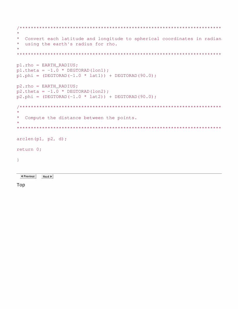
/****************************************************************************** ** Convert each latitude and longitude to spherical coordinates in radians ** using the earth's radius for rho. ** ******************************************************************************/
p1.rho = EARTH_RADIUS;p1.theta = -1.0 * DEGTORAD(lon1);p1.phi = (DEGTORAD(-1.0 * lat1)) + DEGTORAD(90.0);
p2.rho = EARTH_RADIUS;p2.theta = -1.0 * DEGTORAD(lon2);p2.phi = (DEGTORAD(-1.0 * lat2)) + DEGTORAD(90.0);
/****************************************************************************** ** Compute the distance between the points. ** ******************************************************************************/
arclen(p1, p2, d);
return 0;
}
Top

Mastering Algorithms with CBy Kyle Loudon
Slots : 1
Table of Contents
Chapter 17. Geometric Algorithms
Content
17.11 Questions and Answers
Q: One application of geometric algorithms mentioned at the start of this chapter was determiningwhether the track of an object transgresses a restricted region. If we assume that the track we followbegins outside of the restricted region, a simple approach to this problem is to determine whetherany line segment in the track intersects with any line segment defining the restricted region. What isthe running time of this approach if we use the lint operation presented in this chapter?
A: The runtime complexity of this approach is O (nm), where n is the number of line segments in thetrack and m is the number of line segments defining the restricted region. This is because for each ofthe n line segments in the track, we call lint once for each of the m line segments in the restrictedregion. Since lint runs in a constant amount of time, the runtime complexity of the solution overall isO (nm).
Q: Determining the orientation of two points with respect to a third is an important part of thealgorithms presented for determining whether line segments intersect and computing convex hulls.Formally, given points p1 , p2, and p3, we determine the orientation of p3 relative to p2 with respectto p1 by treating the line segments from p1 to p2 and p1 to p3 as vectors U and V. We then use thesign of the z-component of the cross product U x V as a gauge of orientation. What is the orientationof the points if we compute the cross product V x U? In other words, given a specific orientation of p3
relative to p2, what is the orientation of p2 relative to p3?
A: The answer to this question is a matter of perspective. Imagine two people facing forward in aroom with a door behind them. Unless the two individuals line up perfectly with the door (one in frontof the other), person A will see person B to his left, whereas person B will see person A to his right,and vice versa. The neat thing about cross products is that they reflect this perspectivemathematically. When we compute the orientation of p 3 relative to p 2 with respect to p1, we get anindication of where p 3 is from the perspective of p 2. For example, p 3 may be clockwise from p 2.When we compute the orientation of p 2 relative to p 3, we get an indication of where p 2 is from theperspective of p 3. These perspectives are always equal but opposite to one another (except in theboundary case when p 2 and p 3 form a straight line with p1). That is, U x V is always equal to but ofopposite sign as V x U (if p 2 and p 3 form a straight line with p 1, U x V and V x U are both 0, andthe line segments from p1 to p 2 and p1 to p 3 are collinear). The formula given earlier in the chapterfor z1 when testing for intersecting line segments comes from U x V. To compute V x U, weexchange the positions of x2 and x3 and of y2 and y3 in the formula. This yields an equivalent resultbut with the sign reversed. Therefore, if p 3 is clockwise from p 2, for example, this tells us that p 2 iscounterclockwise from p 3, as we would expect.

Q: To test whether two line segments from points p1 to p2 and p3 to p4 intersect, we first examinewhether the bounding boxes of the line segments intersect and then compare the orientation of p3
relative to p2 with that of p4 relative to p2. In what situation do the bounding boxes intersect whenthe orientations of both p3 and p4 are 0? Is it possible to have bounding boxes that do not intersectwhen the orientations of p3 and p4 are both 0?
A: Recall that when the orientation of either p 3 or p4 is 0, it means that the line segment from eitherp1 to p 3 or p1 to p4 is collinear with the line segment from p1 to p 2. If the bounding boxes of the twoline segments intersect as well, this tells us that at least some parts of the segments overlay eachother (see Figure 17.9a). Therefore, the line segments intersect. On the other hand, it is possible tohave two line segments that are collinear without intersecting. This occurs when the segments wouldoverlay each other if either were long enough, but neither has the length necessary to do so (seeFigure 17.9b).
Figure 17.9. Collinear line segments whose bounding boxes (a) intersectand (b) do not intersect
Q: In this chapter we learned that the smallest polygon surrounding a set of points is called a convexhull. This name implies that the polygon is always convex. Why is this?
A: Recall that a polygon is convex if any line segment connecting two points inside the polygon liescompletely inside the polygon itself; otherwise, the polygon is concave. To understand why a convexhull is always convex, consider a concave polygon that surrounds a set of points. For any sequence ofthree points p1, p 2, and p 3 defining a concave region, if we replace the edges from p1 to p 2 and p 2to p 3 with a single edge from p1 to p 3, we can reduce the size of the polygon while keeping p 2enclosed. We know that the size of the polygon will be reduced because it is always shorter to gofrom one point to another than through a third point first. We know that p 2 will still be enclosed bythe resulting polygon because the angle from p 2 to p 3 is less than the angle from p1 to p 2.Therefore, since a convex polygon will always be shorter than any concave one that encloses thesame points, a convex hull must be convex (see Figure 17.10).
Figure 17.10. Showing that the smallest polygon enclosing a set of pointsis always convex

Q: Suppose in the approximation for distances on Earth presented in this chapter we would like toimprove the method used in the function geodist. Specifically, we would like to do something to takeinto account the change in the Earth's radius at different latitudes and longitudes. How can we dothis?
A: One way to make this improvement is to use the fact that both points passed into geodist havetheir own value for the spherical coordinate r. When we treat the Earth as a perfect sphere, we setthe rho member of each point to the same value since we are considering the distance from theEarth's center to the surface to be the same everywhere. However, a better approach would be toset rho for each point to the actual distance from the center of the Earth to the point and thencompute an average of the two rho members for the radius of the arc. Although this does notperfect the distance computation, it does generally improve it.
Top

Mastering Algorithms with CBy Kyle Loudon
Slots : 1
Table of Contents
Chapter 17. Geometric Algorithms
Content
17.12 Related Topics
Vectors
Mathematical quantities having both magnitude and direction. A vector consists of severalcomponents , one for each axis of the coordinate system. If we draw a vector as a linesegment starting at the origin, a vector's components are values that describe how far wemust move along each axis to reach the point at which the vector ends. Some operations withvectors include addition, subtraction, dot products, cross products, and magnitudes.
Testing whether any two line segments intersect
A generalization of the test provided earlier in this chapter for determining whether two linesegments intersect. However, rather than simply applying this test over and over again to testwhether any line segments in a set intersect, it is best to use a dedicated approach. Using adedicated approach, the problem can be solved in O (n lg n) time, where n is the number ofline segments.
Graham's scan
An alternative approach to Jarvis's march for computing convex hulls. Graham's scan works bymaintaining a stack of candidate points for the convex hull. Each point is pushed onto the stackonce. All points not in the convex hull are eventually popped off the stack so that when thealgorithm terminates, the stack contains only the points in the convex hull. Graham's scan hasa runtime complexity of O (n lg n), where n is the number of points in the set to enclose.
Top

Mastering Algorithms with CBy Kyle Loudon
Slots : 1
Table of Contents
Content
Colophon
Our look is the result of reader comments, our own experimentation, and feedback from distributionchannels. Distinctive covers complement our distinctive approach to technical topics, breathingpersonality and life into potentially dry subjects.
The animals on the cover of Mastering Algorithms with C are sea horses. Sea horses are of the familySyngnathidae, genus Hippocampus. The word "hippocampus" comes from the Greek for "bent horse."The sea horse's unusual-looking body is formed by 50 or so bony plates that encircle the body tocreate rings of armor. Within their narrow snouts are tubes through which they feed, sucking inplankton and tiny fish larvae. The male sea horse has a pouch in his belly, into which a female lays100 or more eggs at a time. The male fertilizes the eggs in the pouch and carries them until theyhatch, ten days to six weeks later, depending on the sea horse species.
Sea horses are found mostly in shallow tropical and subtropical waters, although there are someocean-dwelling sea horse species. All sea horses use their pelvic and pectoral fins for steering. Theyswim slowly, in an upright position, and take frequent breaks. During these breaks they wrap theirprehensile tails around a piece of seaweed or coral to anchor themselves. In addition to providing aresting place, the seaweed and coral provide good camouflage for the sea horse.
The largest sea horse species is the Pacific sea horse, measuring approximately 12 inches long. Thesmallest is the dwarf sea horse, which measures only an inch and a half long.
Jeffrey Liggett was the production editor for Mastering Algorithms with C; Cindy Kogut was thecopyeditor; Ellie Fountain Maden was the proofreader; Sebastian Banker provided productionassistance; Claire Cloutier LeBlanc, Nancy Wolfe Kotary, and Melanie Wang provided quality control.Robert Romano and Rhon Porter created the illustrations using Adobe Photoshop 5 and MacromediaFreeHand 8. Mike Sierra provided FrameMaker technical support. William Meyers wrote the indexwith production assistance by Seth Maislin and Brenda Miller.
Hanna Dyer designed the cover of this book based on a series design by Edie Freedman. Theillustration is by Lorrie LeJeune. The cover layout was produced by Kathleen Wilson with QuarkXPress3.32 using the ITC Garamond font. Kathleen Wilson designed the diskette label.
The inside layout was designed by Alicia Cech based on a series design by Nancy Priest. The insidelayout was implemented in FrameMaker 5.5.6 by Mike Sierra. The text and heading fonts are ITCGaramond Light and Garamond Book. This colophon was written by Clairemarie Fisher O'Leary.
The online edition of this book was created by the Safari production group (John Chodacki, Becki

Maisch, and Madeleine Newell) using a set of Frame-to-XML conversion and cleanup tools written andmaintained by Erik Ray, Benn Salter, John Chodacki, and Jeff Liggett.
Top

Mastering Algorithms with C
By Kyle Loudon
Slots : 1
Table of Contents
[SYMBOL] [A] [B] [C] [D] [E] [F] [G] [H] [I] [J] [K] [L] [M] [N] [O] [P] [Q] [R] [S] [T] [U] [V] [W] [X]
Top