This is an Open Access document downloaded from ORCA, Cardiff University's institutional

repository: http://orca.cf.ac.uk/80519/

This is the author’s version of a work that was submitted to / accepted for publication.

Citation for final published version:

Yokoi, Kensuke, Onishi, Ryo, Deng, Xiao-Long and Sussman, Mark 2016. Density-scaled balanced

continuum surface force model with a level set based curvature interpolation technique.

International Journal of Computational Methods 13 (4) 10.1142/S0219876216410048 file

Publishers page: http://dx.doi.org/10.1142/S0219876216410048

<http://dx.doi.org/10.1142/S0219876216410048>

Please note:

Changes made as a result of publishing processes such as copy-editing, formatting and page

numbers may not be reflected in this version. For the definitive version of this publication, please

refer to the published source. You are advised to consult the publisher’s version if you wish to cite

this paper.

This version is being made available in accordance with publisher policies. See

http://orca.cf.ac.uk/policies.html for usage policies. Copyright and moral rights for publications

made available in ORCA are retained by the copyright holders.

Density-scaled balanced continuum surface force model with a level

set based curvature interpolation technique

Kensuke Yokoi1∗, Ryo Onishi2, Xiao-Long Deng3, Mark Sussman4

1School of Engineering, Cardiff University, The Parade, Cardiff, CF24 3AA, UK2Center for Earth Information Science and Technology,

Japan Agency for Marine-Earth Science and Technology, Yokohama, 236-0001, Japan3Beijing Computational Science Research Center, Beijing, China

4Department of Mathematics, Florida State University, Tallahassee, FL, USA

September 23, 2015

Abstract

We examine the recently-proposed density-scaled balanced CSF (continuum surface force) model with a level

set based curvature interpolation technique. The density-scaled balanced CSF model is combined with a numerical

framework which is based on the CLSVOF (coupled level set and volume-of-fluid) method, the THINC/WLIC (tangent

of hyperbola for interface capturing/weighted line interface calculation) scheme, multi-moment methods (CIP-CSLR

and VSIAM3). The present CSF model is examined for various bench mark problems such as drop-drop collisions

and drop splashing. Comparisons of the present model results with experimental observations and those from the

other CSF models show that the present CSF model can minimize spurious current and capture complicated fluid

phenomena with minimizing floatsam.

keywords: CSF model; density-scaling; CLSVOF method; surface tension; drop splashing

1 Introduction

Various surface tension force models have been proposed [3, 12, 11, 16, 13, 7, 19, 20, 15, 2] for a wide variety

of scientific and industrial applications. Examples are drop-drop collisional breakups and sea spray generations for

geoscience; fuel atomizations and bubble column reactors for industries. The CSF model by Brackbill et al. [3] has

widely been used as a surface tension model. A density scaling of the CSF model has also been proposed in the

original CSF model paper [3] and detailed in a following paper [12]. The density scaling improves stability of surface

tension force computations [4, 7, 40]. Recently the balanced force algorithm [7, 2] has gained a popularity because

the algorithm can reduce spurious currents. The ghost fluid or sharp interface approaches [11, 13, 19, 5, 42] have also

widely been used in surface tension force computations. However if the ghost fluid or sharp interface approaches are

used on a regular Cartesian grid, the numerical results have relatively strong influences by the grid geometry. Therefore,

we focus only on CSF formulations in this paper.

A numerical framework which can simulate drop splashing has been proposed in [40]. The framework employs

the density-scaled CSF model as the surface tension force model. However the framework has a crucial issue that it

generates relatively large spurious currents that cause unphysical behaviors in some parameter ranges and situations

(e.g., for very low Bond number). Although it is well known that the balanced CSF formulation can minimize spurious

∗Corresponding author: School of Engineering, Cardiff University, The Parade, Cardiff, CF24 3AA, UK. Tel: +44 (0)29 20870844, Fax: +44

(0)29 20874716, email:YokoiK@cardiff.ac.uk.

1

currents [7, 2], the conventional balanced CSF model, without using the density-scaling, cannot well capture drop

splashing (satellite droplets) as will be discussed in [40]. Therefore, in this paper, we employ a density-scaled CSF

model within the balanced force formulation (hereafter refereed to as density-scaled balanced CSF model) which can

possibly take both advantages of the density-scaling and balanced force formulation. A preliminary result of the

proposed numerical algorithm has already been published in [41] as a short note. In this paper, we report further details

of numerical results. Although a density-scaled balanced CSF model was discussed in the original paper of the balanced

force formulation [7], the model was examined in a limited situation (when the exact curvature is given and very small

pressure tolerance is used). Consequently it was concluded that the density-scaled balanced CSF model would be less

capable than the standard balanced CSF model. In this paper, we further examine the details of the density-scaled

balanced CSF model and show that the density-scaled balanced CSF model actually can reduce spurious currents more

than the standard balanced CSF model when the exact curvature is not give (this is, in fact, the common practical

situation).

The density-scaled balanced CSF model is combined with a fluid framework which consists of the CLSVOF

method, THINC/WLIC scheme, CIP-CSLR (constrained interpolation profile conservative semi-Lagrangian with ra-

tional function) method [23, 33, 26] and VSIAM3 (volume/surface integrated average based multi-moment method)

[27, 29]. The fluid framework has been validated through various test problems and applications in [36, 37, 38, 39, 40].

The proposed CSF model is validated through two benchmark problems (equilibrium drop and single bubble rising).

We also conduct numerical simulations of binary drop collisions and drop splashing on a superhydrophobic substrate,

and compare the results with experimental observations. The comparisons show that the numerical framework can

minimize spurious currents, and also well capture the physics of binary drop collisions and drop splashing.

2 Numerical method

2.1 Numerical framework for free surface flows

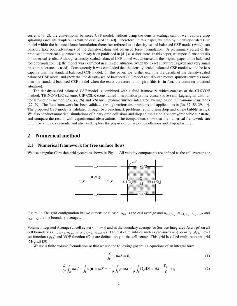
We use a regular Cartesian grid system as shown in Fig. 1. All velocity components are defined as the cell average (or

u ,v ,pu,v

Ω

Γ

i,ji-1/2,j i+1/2,j

i,j+1/2

i,j-1/2

u,v

u,v

u,v

Figure 1: The grid configuration in two dimensional case. ui, j is the cell average and ui−1/2, j, ui+1/2, j, vi, j−1/2 and

vi, j+1/2 are the boundary averages.

Volume Integrated Average) at cell center (ui, j,vi, j) and as the boundary average (or Surface Integrated Average) on all

cell boundaries (ui−1/2, j, ui, j−1/2 ,vi−1/2, j, vi, j−1/2). The rest of quantities such as pressure (pi, j), density (ρi, j), level

set function (ψi, j) and VOF function (Ci, j) are defined only at the cell center. This grid is called multi-moment grid

(M-grid) [30].

We use a finite volume formulation so that we use the following governing equations of an integral form,

∫

Γu ·ndS = 0, (1)

∂

∂ t

∫

ΩudV +

∫

Γu(u ·n)dS =−

1

ρ

∫

ΓpndS+

1

ρ

∫

Γ(2µD) ·ndS+

Fs f

ρ+g (2)

2

where u is the velocity, n the outgoing normal vector for the control volume Ω with its surface denoted by Γ (see Fig.

1), ρ the density, p the pressure, D the deformation tensor (D = 0.5(∇u+(∇u)T )), Fs f the surface tension force and g

the acceleration due to the gravity. Equations (1) and (2) are solved by a multi-moment method based on the CIP-CSLR

method [26] and VSIAM3 [27, 29]. For interface capturing, we use the CLSVOF method [21] with the THINC/WLIC

method [28, 36, 37]. For more details including the contact angle implementation, see [37, 38, 40, 22].

2.2 Surface tension force model

The surface tension force, Fs f , appears as the surface force

Fs f = σκns, (3)

where σ is the fluid surface tension coefficient, κ the local mean curvature and ns is the unit vector normal to the liquid

interface. In the CSF formulation [3], the surface tension force is modeled as a body force associated by a smoothed

delta function δα

Fs f = σκδα ns. (4)

2.2.1 Level set based, not density-scaled, delta function, CSF model

In the level set formulation [17], the gradient of the level set function ψ is used as the surface normal

Fs f = σκδα(ψ)nls. (5)

with

nls =∇ψ

|∇ψ|. (6)

The curvature κ is computed as

κ =−∇ ·nls. (7)

The smoothed delta function δα(ψ) can also be obtained from the level set function as

δα(ψ) =

12α [1+ cos(πψ

α )] if |ψ|< α0 else .

(8)

The corresponding smoothed Heaviside function of (8) is

Hα(ψ) =

0 if ψ <−α12[1+ ψ

α + 1π sin(πψ

α )] if |ψ| ≤ α1 if ψ > α.

(9)

and satisfies the relationdHα (ψ)

dψ = δα(ψ). The smoothed Heaviside function (9) is the same with the smoothed Heavi-

side function to generate the density function φ :

φi, j = Hα(ψi, j). (10)

The x-component of acceleration due to (5) is discretized as

(Fs f

ρ)i−1/2, j =

σκi−1/2, j

ρi−1/2, jδα(ψi−1/2, j)nls,x,i−1/2, j, (11)

here

nls,x,i−1/2, j =1

2(nls,x,i−1/2, j−1/2 +nls,x,i−1/2, j+1/2), (12)

nls,x,i−1/2, j−1/2 =ψx,i−1/2, j−1/2

√

ψ2x,i−1/2, j−1/2

+ψ2y,i−1/2, j−1/2

, (13)

ψx,i−1/2, j−1/2 =1

2(

ψi, j −ψi−1, j

∆x+

ψi, j−1 −ψi−1, j−1

∆x). (14)

This is the standard CSF model based on the level set method [17].

3

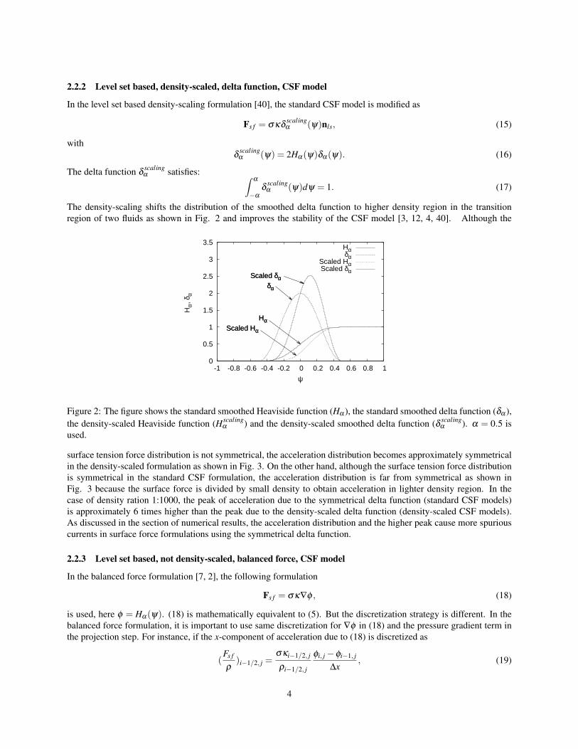
2.2.2 Level set based, density-scaled, delta function, CSF model

In the level set based density-scaling formulation [40], the standard CSF model is modified as

Fs f = σκδscalingα (ψ)nls, (15)

with

δscalingα (ψ) = 2Hα(ψ)δα(ψ). (16)

The delta function δscalingα satisfies:

∫ α

−αδ scaling

α (ψ)dψ = 1. (17)

The density-scaling shifts the distribution of the smoothed delta function to higher density region in the transition

region of two fluids as shown in Fig. 2 and improves the stability of the CSF model [3, 12, 4, 40]. Although the

0

0.5

1

1.5

2

2.5

3

3.5

-1 -0.8 -0.6 -0.4 -0.2 0 0.2 0.4 0.6 0.8 1

Hα,

δα

ψ

δα

Scaled δα

HαScaled Hα

δα

Scaled δα

HαScaled Hα

Hαδα

Scaled HαScaled δα

Figure 2: The figure shows the standard smoothed Heaviside function (Hα ), the standard smoothed delta function (δα ),

the density-scaled Heaviside function (Hscalingα ) and the density-scaled smoothed delta function (δ

scalingα ). α = 0.5 is

used.

surface tension force distribution is not symmetrical, the acceleration distribution becomes approximately symmetrical

in the density-scaled formulation as shown in Fig. 3. On the other hand, although the surface tension force distribution

is symmetrical in the standard CSF formulation, the acceleration distribution is far from symmetrical as shown in

Fig. 3 because the surface force is divided by small density to obtain acceleration in lighter density region. In the

case of density ration 1:1000, the peak of acceleration due to the symmetrical delta function (standard CSF models)

is approximately 6 times higher than the peak due to the density-scaled delta function (density-scaled CSF models).

As discussed in the section of numerical results, the acceleration distribution and the higher peak cause more spurious

currents in surface force formulations using the symmetrical delta function.

2.2.3 Level set based, not density-scaled, balanced force, CSF model

In the balanced force formulation [7, 2], the following formulation

Fs f = σκ∇φ , (18)

is used, here φ = Hα(ψ). (18) is mathematically equivalent to (5). But the discretization strategy is different. In the

balanced force formulation, it is important to use same discretization for ∇φ in (18) and the pressure gradient term in

the projection step. For instance, if the x-component of acceleration due to (18) is discretized as

(Fs f

ρ)i−1/2, j =

σκi−1/2, j

ρi−1/2, j

φi, j −φi−1, j

∆x, (19)

4

0

5

10

15

20

25

30

-1 -0.5 0 0.5 1

Acc

eler

atio

n du

e to

sur

face

forc

e

ψ

Density-scaled CSFStandard CSF

Figure 3: The figure shows the magnitudes of acceleration due to the standard CSF model and density-scaled CSF

model, when r = 1, κ = 1, α = 0.5 and the density ratio 1:1000.

the x-component of acceleration due to the pressure gradient must be discretized as

(∂u

∂ t)i−1/2, j =−

1

ρi−1/2, j

pn+1i, j − pn+1

i−1, j

∆x, (20)

here ρi−1/2, j ≡12(ρi−1, j +ρi, j). Hereafter the level set based standard balanced CSF model is refereed to as balanced

CSF model.

2.2.4 Level set based, density-scaled, balanced force, CSF model

In the density-scaled balanced CSF model, we define a non-symmetrical smoothed Heaviside function Hscalingα (ψ)

Hscalingα (ψ) =

0 if ψ <−α12[ 1

2+ ψ

α + ψ2

2α2 −1

4π2 (cos( 2πψα )−1)+ α+ψ

απ sin(πψα )] if |ψ| ≤ α

1 if ψ > α,

(21)

as shown in Fig. 2. Here Hscalingα (ψ) satisfies the relation

dHscalingα (ψ)

dψ = δscalingα (ψ). Therefore the formulation is math-

ematically identical to the density-scaled CSF model. However the discretization strategy is different. The acceleration

due to the surface tension force is calculated by taking the gradient of the density function φscalingi, j which is generated

by using Hscalingα (ψi, j) as

(Fs f

ρ)i−1/2, j =

σκi−1/2, j

ρi−1/2, j

φscalingi, j −φ

scalingi−1, j

∆x, (22)

here

φscalingi, j = H

scalingα (ψi, j). (23)

The discretization of (22) is still consistent with (20). That is, this formulation is a balanced force formulation. The

implementation of the density-scaled balanced CSF model is simple and compact. We just need to create a function

(subroutine) to generate φscalingi, j from ψi, j using H

scalingα (ψi, j) and calculate the gradient of φ

scalingi, j as (22).

2.3 Level set based curvature interpolation

Curvature of the interface is typically calculated at cell center. Therefore curvature must be interpolated at cell faces

when updating all the velocity components. In this paper, we use a methodology which interpolates curvature at the

5

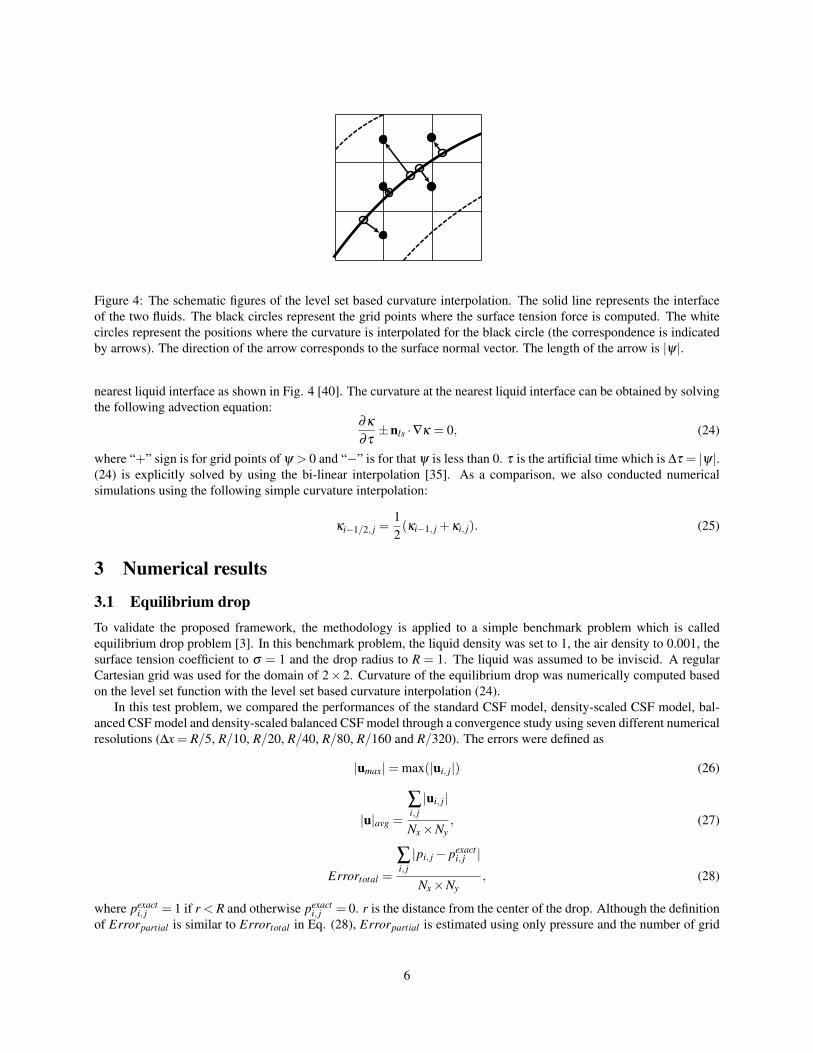
Figure 4: The schematic figures of the level set based curvature interpolation. The solid line represents the interface

of the two fluids. The black circles represent the grid points where the surface tension force is computed. The white

circles represent the positions where the curvature is interpolated for the black circle (the correspondence is indicated

by arrows). The direction of the arrow corresponds to the surface normal vector. The length of the arrow is |ψ|.

nearest liquid interface as shown in Fig. 4 [40]. The curvature at the nearest liquid interface can be obtained by solving

the following advection equation:∂κ

∂τ±nls ·∇κ = 0, (24)

where “+” sign is for grid points of ψ > 0 and “−” is for that ψ is less than 0. τ is the artificial time which is ∆τ = |ψ|.(24) is explicitly solved by using the bi-linear interpolation [35]. As a comparison, we also conducted numerical

simulations using the following simple curvature interpolation:

κi−1/2, j =1

2(κi−1, j +κi, j). (25)

3 Numerical results

3.1 Equilibrium drop

To validate the proposed framework, the methodology is applied to a simple benchmark problem which is called

equilibrium drop problem [3]. In this benchmark problem, the liquid density was set to 1, the air density to 0.001, the

surface tension coefficient to σ = 1 and the drop radius to R = 1. The liquid was assumed to be inviscid. A regular

Cartesian grid was used for the domain of 2×2. Curvature of the equilibrium drop was numerically computed based

on the level set function with the level set based curvature interpolation (24).

In this test problem, we compared the performances of the standard CSF model, density-scaled CSF model, bal-

anced CSF model and density-scaled balanced CSF model through a convergence study using seven different numerical

resolutions (∆x = R/5, R/10, R/20, R/40, R/80, R/160 and R/320). The errors were defined as

|umax|= max(|ui, j|) (26)

|u|avg =

∑i, j

|ui, j|

Nx ×Ny

, (27)

Errortotal =

∑i, j

|pi, j − pexacti, j |

Nx ×Ny

, (28)

where pexacti, j = 1 if r < R and otherwise pexact

i, j = 0. r is the distance from the center of the drop. Although the definition

of Errorpartial is similar to Errortotal in Eq. (28), Errorpartial is estimated using only pressure and the number of grid

6

points, in areas of r < R/2 and r > 3R/2. Errorpartial measures the pressure errors without including errors around the

smoothed interface.

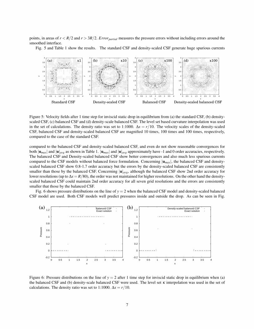
Fig. 5 and Table 1 show the results. The standard CSF and density-scaled CSF generate huge spurious currents

0

0.5

1

1.5

2

2.5

3

3.5

4

0 0.5 1 1.5 2 2.5 3 3.5 4

y

x

0

0.5

1

1.5

2

2.5

3

3.5

4

0 0.5 1 1.5 2 2.5 3 3.5 4

y

x

0

0.5

1

1.5

2

2.5

3

3.5

4

0 0.5 1 1.5 2 2.5 3 3.5 4

y

x

Density-scaled CSF Balanced CSF Density-scaled balanced CSF

x100 x100

0

0.5

1

1.5

2

2.5

3

3.5

4

0 0.5 1 1.5 2 2.5 3 3.5 4

y

x

Standard CSF

x10x1(a) (b) (c) (d)

Figure 5: Velocity fields after 1 time step for inviscid static drop in equilibrium from (a) the standard CSF, (b) density-

scaled CSF, (c) balanced CSF and (d) density-scale balanced CSF. The level set based curvature interpolation was used

in the set of calculations. The density ratio was set to 1:1000. ∆x = r/10. The velocity scales of the density-scaled

CSF, balanced CSF and density-scaled balanced CSF are magnified 10 times, 100 times and 100 times, respectively,

compared to the case of the standard CSF.

compared to the balanced CSF and density-scaled balanced CSF, and even do not show reasonable convergences for

both |umax| and |u|avg as shown in Table 1. |umax| and |u|avg approximately have -1 and 0 order accuracies, respectively.

The balanced CSF and Density-scaled balanced CSF show better convergences and also much less spurious currents

compared to the CSF models without balanced force formulation. Concerning |umax|, the balanced CSF and density-

scaled balanced CSF show 0.8-1.7 order accuracy but the errors by the density-scaled balanced CSF are consistently

smaller than those by the balanced CSF. Concerning |u|avg, although the balanced CSF show 2nd order accuracy for

lower resolutions (up to ∆x=R/80), the order was not maintained for higher resolutions. On the other hand the density-

scaled balanced CSF could maintain 2nd order accuracy for all seven grid resolutions and the errors are consistently

smaller that those by the balanced CSF.

Fig. 6 shows pressure distributions on the line of y = 2 when the balanced CSF model and density-scaled balanced

CSF model are used. Both CSF models well predict pressures inside and outside the drop. As can be seen in Fig.

-0.2

0

0.2

0.4

0.6

0.8

1

1.2

0 0.5 1 1.5 2 2.5 3 3.5 4

Pre

ssur

e

x

Balanced CSFExact solution

-0.2

0

0.2

0.4

0.6

0.8

1

1.2

0 0.5 1 1.5 2 2.5 3 3.5 4

Pre

ssur

e

x

Density-scaled balanced CSFExact solution

(a) (b)

Figure 6: Pressure distributions on the line of y = 2 after 1 time step for inviscid static drop in equilibrium when (a)

the balanced CSF and (b) density-scale balanced CSF were used. The level set κ interpolation was used in the set of

calculations. The density ratio was set to 1:1000. ∆x = r/10.

7

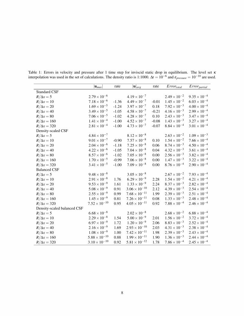
Table 1: Errors in velocity and pressure after 1 time step for inviscid static drop in equilibrium. The level set κinterpolation was used in the set of calculations. The density ratio is 1:1000. ∆t = 10−6 and εpressure = 10−10 are used.

|umax| rate |u|avg rate Errortotal Errorpartial

Standard CSF

R/∆x = 5 2.79×10−6 4.19×10−7 2.49×10−2 9.35×10−4

R/∆x = 10 7.18×10−6 -1.36 4.49×10−7 -0.01 1.45×10−2 6.03×10−4

R/∆x = 20 1.69×10−5 -1.24 3.97×10−7 0.18 7.92×10−3 4.00×10−4

R/∆x = 40 3.49×10−5 -1.05 4.58×10−7 -0.21 4.16×10−3 2.99×10−4

R/∆x = 80 7.06×10−5 -1.02 4.28×10−7 0.10 2.43×10−3 3.47×10−4

R/∆x = 160 1.41×10−4 -1.00 4.52×10−7 -0.08 1.43×10−3 3.27×10−4

R/∆x = 320 2.81×10−4 -1.00 4.73×10−7 -0.07 8.84×10−4 3.01×10−4

Density-scaled CSF

R/∆x = 5 4.84×10−7 8.12×10−8 2.63×10−2 1.09×10−3

R/∆x = 10 9.01×10−7 -0.90 7.57×10−8 0.10 1.54×10−2 7.66×10−4

R/∆x = 20 2.04×10−6 -1.18 7.25×10−8 0.06 8.74×10−3 4.50×10−4

R/∆x = 40 4.22×10−6 -1.05 7.04×10−8 0.04 4.32×10−3 3.61×10−4

R/∆x = 80 8.57×10−6 -1.02 7.05×10−8 0.00 2.56×10−3 3.82×10−4

R/∆x = 160 1.70×10−5 -0.99 7.06×10−8 0.00 1.47×10−3 3.22×10−4

R/∆x = 320 3.41×10−5 -1.00 7.09×10−8 0.00 8.76×10−4 2.90×10−4

Balanced CSF

R/∆x = 5 9.48×10−8 3.05×10−8 2.67×10−2 7.93×10−4

R/∆x = 10 2.91×10−8 1.76 6.29×10−9 2.28 1.54×10−2 4.21×10−4

R/∆x = 20 9.53×10−9 1.61 1.33×10−9 2.24 8.37×10−3 2.82×10−4

R/∆x = 40 5.08×10−9 0.91 3.06×10−10 2.12 4.39×10−3 2.54×10−4

R/∆x = 80 2.55×10−9 0.99 7.68×10−11 1.99 2.39×10−3 2.51×10−4

R/∆x = 160 1.45×10−9 0.81 7.26×10−11 0.08 1.33×10−3 2.48×10−4

R/∆x = 320 7.52×10−10 0.95 4.05×10−11 0.92 7.88×10−4 2.46×10−4

Density-scaled balanced CSF

R/∆x = 5 6.68×10−8 2.02×10−8 2.68×10−2 6.88×10−4

R/∆x = 10 2.29×10−8 1.54 5.00×10−9 2.01 1.56×10−2 3.72×10−4

R/∆x = 20 6.97×10−9 1.72 1.20×10−9 2.06 8.83×10−3 2.52×10−4

R/∆x = 40 2.16×10−9 1.69 2.93×10−10 2.03 4.31×10−3 2.38×10−4

R/∆x = 80 1.08×10−9 1.00 7.42×10−11 1.98 2.39×10−3 2.43×10−4

R/∆x = 160 5.88×10−10 0.88 1.99×10−11 1.90 1.36×10−3 2.44×10−4

R/∆x = 320 3.10×10−10 0.92 5.81×10−12 1.78 7.86×10−4 2.45×10−4

8

Table 2: Errors in velocity and pressure after 1 time step for inviscid static drop in equilibrium. The simple κ interpo-

lation was used in the set of calculations. The density ratio was set to 1:1000. ∆t = 10−6 is used.

|umax| rate |u|avg rate Errortotal Errorpartial

Balanced CSF

R/∆x = 5 1.41×10−7 2.28×10−8 2.82×10−2 2.44×10−2

R/∆x = 10 2.31×10−7 -0.71 1.46×10−8 0.64 1.59×10−2 5.83×10−3

R/∆x = 20 2.96×10−7 -0.36 9.30×10−9 0.65 8.54×10−3 1.33×10−3

R/∆x = 40 3.23×10−7 -0.13 5.14×10−9 0.86 4.39×10−3 1.85×10−4

Density-scaled balanced CSF

R/∆x = 5 8.88×10−8 2.08×10−8 3.45×10−2 8.94×10−2

R/∆x = 10 5.15×10−8 0.79 4.80×10−9 2.12 2.01×10−2 3.72×10−2

R/∆x = 20 5.70×10−8 -0.15 1.96×10−9 1.29 1.14×10−2 1.67×10−2

R/∆x = 40 6.04×10−8 -0.08 1.08×10−9 0.86 5.66×10−3 7.85×10−3

6, pressure distributions by these CSF models in the transition region are different because surface force distributions

by these CSF models in the transition region are different. Concerning errors in pressure (Errortotal), all four CSF

models generate similar errors as shown in Table 1 because the smoothed interfaces generate large errors in pressure

calculations due to the nature of CSF models. Therefore it is difficult to see differences among these four CSF models

based on Errortotal . Therefore we defined Errorpartial which does not involve errors in pressure around the smoothed

interfaces. As shown in Table 1, Errorpartial by the density-scaled balanced CSF model is smaller than that by the

balanced CSF model. The standard CSF model and density-scaled CSF model generate larger Errorpartial than the

balanced CSF model and density-scaled balanced CSF model.

We also examine performances of two curvature interpolation strategies, i.e. the level set based curvature inter-

polation (Eq. 24) and simple curvature interpolation (Eq. 25). In previous numerical simulations, the level set based

curvature interpolation (Eq. 24) was used. Table 2 and Fig. 7 show the results when the simple curvature interpolation

(25) was used. If the simple curvature interpolation is used, most of the errors are increased as shown in Table 2.

-0.2

0

0.2

0.4

0.6

0.8

1

1.2

0 0.5 1 1.5 2 2.5 3 3.5 4

Pre

ssur

e

x

Balanced CSFExact solution

(a)

-0.2

0

0.2

0.4

0.6

0.8

1

1.2

0 0.5 1 1.5 2 2.5 3 3.5 4

Pre

ssur

e

x

Density-scaled balanced CSFExact solution

(b)

Figure 7: Pressure distributions on the line of y = 2 when the balanced CSF and density-scaled balanced CSF were

used with the standard κ interpolation for the static drop problem.

If the simple curvature interpolation is used, |umax| do not show convergence even though the balanced CSF model

and density-scaled balanced CSF model are used. Errorpartial by the density-scaled CSF model becomes significantly

larger as also shown in Fig. 7. This is because, in the density-scaled formulation, the surface tension force distribution

is shifted to the higher density region (i.e. the surface force distribution is slightly shifted to inside of the drop in this

9

test problem). Then, if the simple curvature interpolation technique (25) is used, curvature slightly inside the drop

interface is used for the surface tension force computation and the error in the curvature calculation causes overesti-

mation of pressure inside the drop. This may be a reason why the density-scaling has not been paid much attention

for a long time. Thus an appropriate curvature interpolation technique must be used for CSF models, particularly for

density-scaled CSF models.

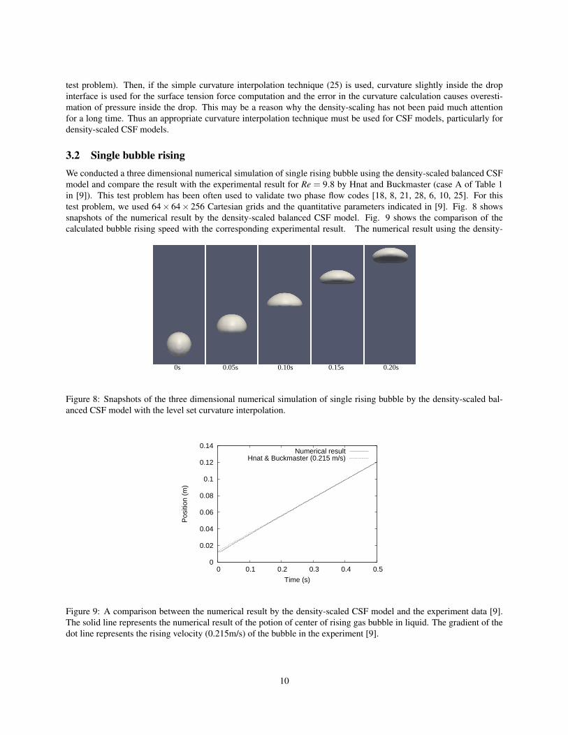
3.2 Single bubble rising

We conducted a three dimensional numerical simulation of single rising bubble using the density-scaled balanced CSF

model and compare the result with the experimental result for Re = 9.8 by Hnat and Buckmaster (case A of Table 1

in [9]). This test problem has been often used to validate two phase flow codes [18, 8, 21, 28, 6, 10, 25]. For this

test problem, we used 64× 64× 256 Cartesian grids and the quantitative parameters indicated in [9]. Fig. 8 shows

snapshots of the numerical result by the density-scaled balanced CSF model. Fig. 9 shows the comparison of the

calculated bubble rising speed with the corresponding experimental result. The numerical result using the density-

0s 0.05s 0.10s 0.15s 0.20s

Figure 8: Snapshots of the three dimensional numerical simulation of single rising bubble by the density-scaled bal-

anced CSF model with the level set curvature interpolation.

0

0.02

0.04

0.06

0.08

0.1

0.12

0.14

0 0.1 0.2 0.3 0.4 0.5

Pos

ition

(m

)

Time (s)

Numerical resultHnat & Buckmaster (0.215 m/s)

Figure 9: A comparison between the numerical result by the density-scaled CSF model and the experiment data [9].

The solid line represents the numerical result of the potion of center of rising gas bubble in liquid. The gradient of the

dot line represents the rising velocity (0.215m/s) of the bubble in the experiment [9].

10

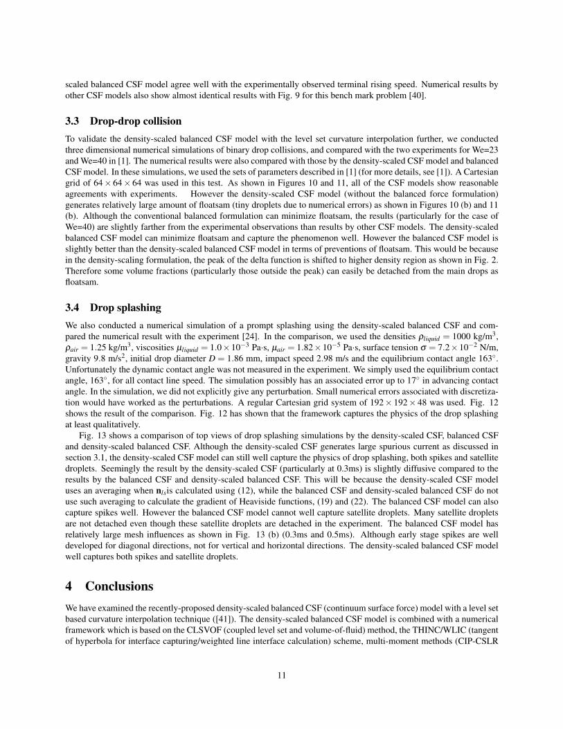
scaled balanced CSF model agree well with the experimentally observed terminal rising speed. Numerical results by

other CSF models also show almost identical results with Fig. 9 for this bench mark problem [40].

3.3 Drop-drop collision

To validate the density-scaled balanced CSF model with the level set curvature interpolation further, we conducted

three dimensional numerical simulations of binary drop collisions, and compared with the two experiments for We=23

and We=40 in [1]. The numerical results were also compared with those by the density-scaled CSF model and balanced

CSF model. In these simulations, we used the sets of parameters described in [1] (for more details, see [1]). A Cartesian

grid of 64× 64× 64 was used in this test. As shown in Figures 10 and 11, all of the CSF models show reasonable

agreements with experiments. However the density-scaled CSF model (without the balanced force formulation)

generates relatively large amount of floatsam (tiny droplets due to numerical errors) as shown in Figures 10 (b) and 11

(b). Although the conventional balanced formulation can minimize floatsam, the results (particularly for the case of

We=40) are slightly farther from the experimental observations than results by other CSF models. The density-scaled

balanced CSF model can minimize floatsam and capture the phenomenon well. However the balanced CSF model is

slightly better than the density-scaled balanced CSF model in terms of preventions of floatsam. This would be because

in the density-scaling formulation, the peak of the delta function is shifted to higher density region as shown in Fig. 2.

Therefore some volume fractions (particularly those outside the peak) can easily be detached from the main drops as

floatsam.

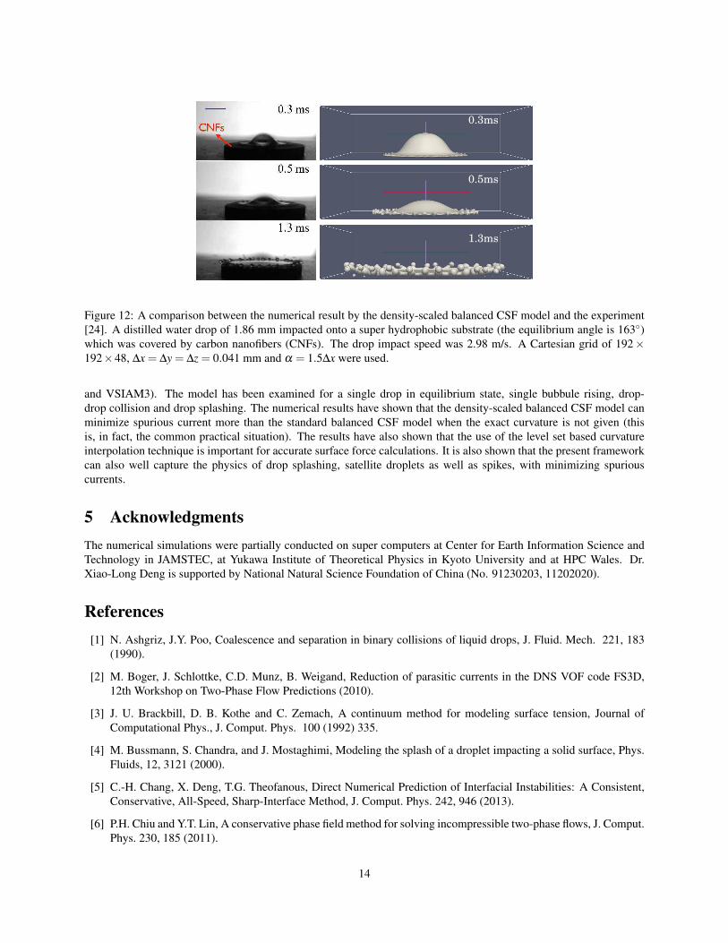
3.4 Drop splashing

We also conducted a numerical simulation of a prompt splashing using the density-scaled balanced CSF and com-

pared the numerical result with the experiment [24]. In the comparison, we used the densities ρliquid = 1000 kg/m3,

ρair = 1.25 kg/m3, viscosities µliquid = 1.0×10−3 Pa·s, µair = 1.82×10−5 Pa·s, surface tension σ = 7.2×10−2 N/m,

gravity 9.8 m/s2, initial drop diameter D = 1.86 mm, impact speed 2.98 m/s and the equilibrium contact angle 163.

Unfortunately the dynamic contact angle was not measured in the experiment. We simply used the equilibrium contact

angle, 163, for all contact line speed. The simulation possibly has an associated error up to 17 in advancing contact

angle. In the simulation, we did not explicitly give any perturbation. Small numerical errors associated with discretiza-

tion would have worked as the perturbations. A regular Cartesian grid system of 192× 192× 48 was used. Fig. 12

shows the result of the comparison. Fig. 12 has shown that the framework captures the physics of the drop splashing

at least qualitatively.

Fig. 13 shows a comparison of top views of drop splashing simulations by the density-scaled CSF, balanced CSF

and density-scaled balanced CSF. Although the density-scaled CSF generates large spurious current as discussed in

section 3.1, the density-scaled CSF model can still well capture the physics of drop splashing, both spikes and satellite

droplets. Seemingly the result by the density-scaled CSF (particularly at 0.3ms) is slightly diffusive compared to the

results by the balanced CSF and density-scaled balanced CSF. This will be because the density-scaled CSF model

uses an averaging when nlsis calculated using (12), while the balanced CSF and density-scaled balanced CSF do not

use such averaging to calculate the gradient of Heaviside functions, (19) and (22). The balanced CSF model can also

capture spikes well. However the balanced CSF model cannot well capture satellite droplets. Many satellite droplets

are not detached even though these satellite droplets are detached in the experiment. The balanced CSF model has

relatively large mesh influences as shown in Fig. 13 (b) (0.3ms and 0.5ms). Although early stage spikes are well

developed for diagonal directions, not for vertical and horizontal directions. The density-scaled balanced CSF model

well captures both spikes and satellite droplets.

4 Conclusions

We have examined the recently-proposed density-scaled balanced CSF (continuum surface force) model with a level set

based curvature interpolation technique ([41]). The density-scaled balanced CSF model is combined with a numerical

framework which is based on the CLSVOF (coupled level set and volume-of-fluid) method, the THINC/WLIC (tangent

of hyperbola for interface capturing/weighted line interface calculation) scheme, multi-moment methods (CIP-CSLR

11

Figure 10: Comparisons among numerical results of binary drop collision (We=23) by the CSF models and the ex-

periment by Ashgriz and Poo [1]. (a) is the experimental result, and (b), (c) and (d) are numerical results by the

density-scaled CSF model, balanced CSF model and density-scaled balanced CSF model, respectively. A Cartesian

grid of 64×64×64 and ∆x = ∆y = ∆z = D/15 (D is the diameter of the initial drops) were used.

12

Figure 11: Comparisons among numerical results of binary drop collision (We=40) by CSF models and the experiment

by Ashgriz and Poo [1]. (a) is the experimental result, and (b), (c) and (d) are numerical results by the density-

scaled CSF model, balanced CSF model and density-scaled balanced CSF model, respectively. A Cartesian grid of

64×64×64 and ∆x = ∆y = ∆z = D/15 were used.

13

0.3ms

0.5ms

1.3ms

Figure 12: A comparison between the numerical result by the density-scaled balanced CSF model and the experiment

[24]. A distilled water drop of 1.86 mm impacted onto a super hydrophobic substrate (the equilibrium angle is 163)

which was covered by carbon nanofibers (CNFs). The drop impact speed was 2.98 m/s. A Cartesian grid of 192×192×48, ∆x = ∆y = ∆z = 0.041 mm and α = 1.5∆x were used.

and VSIAM3). The model has been examined for a single drop in equilibrium state, single bubbule rising, drop-

drop collision and drop splashing. The numerical results have shown that the density-scaled balanced CSF model can

minimize spurious current more than the standard balanced CSF model when the exact curvature is not given (this

is, in fact, the common practical situation). The results have also shown that the use of the level set based curvature

interpolation technique is important for accurate surface force calculations. It is also shown that the present framework

can also well capture the physics of drop splashing, satellite droplets as well as spikes, with minimizing spurious

currents.

5 Acknowledgments

The numerical simulations were partially conducted on super computers at Center for Earth Information Science and

Technology in JAMSTEC, at Yukawa Institute of Theoretical Physics in Kyoto University and at HPC Wales. Dr.

Xiao-Long Deng is supported by National Natural Science Foundation of China (No. 91230203, 11202020).

References

[1] N. Ashgriz, J.Y. Poo, Coalescence and separation in binary collisions of liquid drops, J. Fluid. Mech. 221, 183

(1990).

[2] M. Boger, J. Schlottke, C.D. Munz, B. Weigand, Reduction of parasitic currents in the DNS VOF code FS3D,

12th Workshop on Two-Phase Flow Predictions (2010).

[3] J. U. Brackbill, D. B. Kothe and C. Zemach, A continuum method for modeling surface tension, Journal of

Computational Phys., J. Comput. Phys. 100 (1992) 335.

[4] M. Bussmann, S. Chandra, and J. Mostaghimi, Modeling the splash of a droplet impacting a solid surface, Phys.

Fluids, 12, 3121 (2000).

[5] C.-H. Chang, X. Deng, T.G. Theofanous, Direct Numerical Prediction of Interfacial Instabilities: A Consistent,

Conservative, All-Speed, Sharp-Interface Method, J. Comput. Phys. 242, 946 (2013).

[6] P.H. Chiu and Y.T. Lin, A conservative phase field method for solving incompressible two-phase flows, J. Comput.

Phys. 230, 185 (2011).

14

1.3ms0.5ms0.3ms

1.3ms0.5ms0.3ms

1.3ms0.5ms0.3ms

(a)Density-scaled CSF

(b)Balanced CSF

(c)Density-scaled balanced CSF

Figure 13: A comparison between the numerical results by the density-scaled CSF model, balanced CSF model and

density-scaled balanced CSF model. A Cartesian grid of 192× 192× 48, ∆x = ∆y = ∆z = 0.041 mm and α = 1.5∆x

are used.

15

[7] M.M. Francois, S.J. Cummins, E.D. Dendy, D. B. Kothe, J. M. Sicilian, M. W. Williams, A balanced-force

algorithm for continuous and sharp interfacial surface tension models within a volume tracking framework, J.

Comput. Phys. 213, 141 (2006).

[8] D. Gueyffier, J. Li, A. Nadim, S. Scardovelli, S. Zaleski, Volume of Fluid interface tracking with smoothed surface

stress methods for three-dimensional flows, J. Comput Phys., 152, 423 (1999).

[9] J. G. Hnat and J. D. Buckmaster, Spherical cap bubbles and skirt formation, Phys. Fluids, 19, 182 (1976).

[10] S. Ii, K. Sugiyama, S. Takeuchi, S. Takagi, Y. Matsumoto, F. Xiao, An interface capturing method with a contin-

uous function: The THINC method with multi-dimensional reconstruction, J. Comput. Phys. 231, 2328 (2012).

[11] M. Kang, R.P. Fedkiw, X.D. Liu, A boundary condition capturing method for multiphase incompressible flow, J.

Sci. Comput. 15, 323 (2000).

[12] D. B. Kothe , W.J. Rider , S. J. Mosso , J. S. Brock , J. I. Hochstein, Volume Tracking of Interfaces Having Surface

Tension in Two and Three Dimensions, Technical Report AIAA 96-0859, in: Proceedings of the 34th Aerospace

Sciences Meeting and Exhibit, January 1518, Reno, NV, 1996.

[13] H. Liu, S. Krishnan, S. Marella and H.S. Udaykumar, Sharp interface Cartesian grid method II: A technique for

simulating droplet interactions with surfaces of arbitrary shape J. Comput. Phys. 210, 32 (2005).

[14] S. Osher and J.A. Sethian, Front propagating with curvature-dependent speed: Algorithms based on Hamilton-

Jacobi formulation, J. Comput. Phys. 79, 12 (1988).

[15] M. Raessi, M. Bussmann, and J. Mostaghimi, A semi-implicit finite volume implementation of the CSF method

for treating surface tension in interfacial flows, Int. J. Numer. Meth. Fluid. 59, 1093 (2009).

[16] Y. Renardy and M. Renardy, PROST: A Parabolic Reconstruction of Surface Tension for the Volume-of-Fluid

Method, J. Comput. Phys., 183 400 (2002).

[17] M. Sussman, P. Smereka and S. Osher, A level set approach for capturing solution to incompressible two-phase

flow, J. Comput. Phys. 114, 146 (1994).

[18] M. Sussman and P. Smereka, Axisymmetric free boundary problems, Journal of Fluid Mechanics 341, 269 (1997).

[19] M. Sussman, K.M. Smith, M.Y. Hussaini, M. Ohta, R. Zhi-Wei, A sharp interface method for incompressible

two-phase flows, J. Comput. Phys. 221, 469 (2007).

[20] M. Sussman and M. Ohta, A Stable and Efficient Method for Treating Surface Tension in Incompressible Two-

Phase Flow, SIAM J. Sci. Comput. 31, 2447 (2009).

[21] M. Sussman, E.G. Puckett. ”A coupled level set and volume-of-fluid method for computing 3D and axisymmetric

incompressible two-phase flows”, J. Comput. Phys. 162 301-337 (2000).

[22] M. Sussman, An adaptive mesh algorithm for free surface flows in general geometries, in Adaptive Method of

Lines, (Chapman & Hall/CRC, Boca Raton, 2002).

[23] R. Tanaka, T. Nakamura and T. Yabe, Constructing exactly conservative scheme in a non-conservative form,

Comput. Phys. Commun. 126, 232 (2000).

[24] P. Tsai, S. Pacheco, C. Pirat, L. Lefferts, and D. Lohse, Drop Impact upon Micro- and Nanostructured Superhy-

drophobic Surfaces Langmuir, 25, 12293 (2009).

[25] Y. Wang, S. Simakhina, M. Sussman, A hybrid level set-volume constraint method for incompressible two-phase

flow, J. Comput. Phys. 231, 6438 (2012).

[26] F. Xiao, T. Yabe, X. Peng and H. Kobayashi, Conservative and oscillation-less atmospheric transport schemes

based on rational functions. J. Geophys. Res. 107, 4609 (2002).

16

[27] F. Xiao, A. Ikebata and T. Hasegawa: Numerical simulations of free-interface fluids by a multi integrated moment

method. Computers & Structures, 83, 409-423 (2005).

[28] F. Xiao, Y Honma and T. Kono, A simple algebraic interface capturing scheme using hyperbolic tangent function,

Int. J. Numer. Meth. Fluid. 48, 1023 (2005).

[29] F. Xiao, R. Akoh and S. Ii: Unified formulation for compressible and incompressible flows by using multi inte-

grated moments II: multi-dimensional version for compressible and incompressible flows. J. Comput. Phys., 213,

31-56 (2006).

[30] F. Xiao, X.D. Peng, X.S. Shen, A finite-volume grid using multimoments for geostrophic adjustment, Mon. Wea.

Rev. 134, 2515 (2006).

[31] F. Xiao, S. Ii and C. Chen, Revisit to the THINC scheme: A simple algebraic VOF algorithm, J. Comput. Phys.,

230, 7086 (2011).

[32] T. Yabe, R. Tanaka, T. Nakamura and F. Xiao, An Exactly Conservative Semi-Lagrangian Scheme (CIP-CSL) In

One Dimension Mon. Wea. Rev. 129, 332 (2001).

[33] T. Yabe, F. Xiao and T. Utsumi, Constrained interpolation profile method for multiphase analysis, J Comput.

Phys. 169, 556 (2001).

[34] K. Yokoi, Numerical method for complex moving boundary problems in a Cartesian fixed grid, Phys. Rev. E, 65,

055701(R) (2002).

[35] K. Yokoi, Numerical method for moving solid object in flows, Phys. Rev. E, 67, 045701(R) (2003).

[36] K. Yokoi, Efficient implementation of THINC scheme: a simple and practical smoothed VOF algorithm, J. Comp.

Phys. 226, 1985 (2007).

[37] K. Yokoi, A numerical method for free-surface flows and its application to droplet impact on a thin liquid layer,

J. Sci. Comp., 35, 372 (2008).

[38] K. Yokoi, D. Vadillo, J. Hinch, I. Hutchings, Numerical studies of the influence of the dynamic contact angle on

a droplet impacting on a dry surface, Phys. Fluids, 21, 072102 (2009).

[39] K. Yokoi, Numerical studies of droplet splashing on a dry surface: triggering a splash with the dynamic contact

angle, Soft Matter, 7, 5120 (2011).

[40] K. Yokoi, A practical numerical framework for free surface flows based on CLSVOF method, multi-moment

methods and density-scaled CSF model: Numerical simulations of droplet splashing, J. Comput. Phys., 232, 252

(2013).

[41] K. Yokoi, A density-scaled continuum surface force model within a balanced force formulation, Journal of Com-

putational Physics, J. Comput. Phys., 278, 221 (2014).

[42] M. Zhang, X. Deng, A sharp interface method for SPH, J. Comput. Phys. (doi:10.1016/j.jcp.2015.09.015).

17