Embed Size (px)
Citation preview

This is the author version of an article published as: Hibiki, Takashi and Situ, Rong and Mi, Ye and Ishii, Mamoru (2003) Local Flow Measurements of Vertical Upward Bubbly Flow in an Annulus . International Journal of Heat and Mass Transfer 46(8):pp. 1479-1496. Copyright 2003 Elsevier Accessed from http://eprints.qut.edu.au
T. Hibiki et al. / Local Flow Measurements of Vertical Upward Bubbly Flow in an Annulus
1
Local Flow Measurements of Vertical
Upward Bubbly Flow in an Annulus
Takashi Hibiki a, b, *
, Rong Situ b, Ye Mi
b, Mamoru Ishii
b
a Research Reactor Institute, Kyoto University, Kumatori, Sennan, Osaka 590-0494, Japan
b School of Nuclear Engineering, Purdue University, West Lafayette, IN 47907-1290, USA
* Tel: +81-724-51-2373, Fax.: +81-724-51-2461, Email: [email protected]
Abstract
Local measurements of flow parameters were performed for vertical upward bubbly
flows in an annulus. The annulus channel consisted of an inner rod with a diameter of 19.1
mm and an outer round tube with an inner diameter of 38.1 mm, and the hydraulic equivalent
diameter was 19.1 mm. Double-sensor conductivity probe was used for measuring void
fraction, interfacial area concentration, and interfacial velocity, and Laser Doppler
anemometer was utilized for measuring liquid velocity and turbulence intensity. A total of
20 data sets for void fraction, interfacial area concentration, and interfacial velocity were
acquired consisting of five void fractions, about 0.050, 0.10, 0.15, 0.20, and 0.25, and four
superficial liquid velocities, 0.272, 0.516, 1.03, and 2.08 m/s. A total of 8 data sets for liquid
velocity and turbulence intensity were acquired consisting of five void fractions, about 0.050,
and 0.10, and four superficial liquid velocities, 0.272, 0.516, 1.03, and 2.08 m/s. The
constitutive equations for distribution parameter and drift velocity in the drift-flux model, and
the semi-theoretical correlation for Sauter mean diameter namely interfacial area
T. Hibiki et al. / Local Flow Measurements of Vertical Upward Bubbly Flow in an Annulus
2
concentration, which were proposed previously, were validated by local flow parameters
obtained in the experiment using the annulus.
Key Words: Void fraction, Interfacial area concentration; Bubble size; Liquid velocity;
Turbulence intensity; Double-sensor conductivity probe; Laser Doppler anemometer;
Drift-flux model; Gas-liquid bubbly flow; Multiphase flow; Annulus
T. Hibiki et al. / Local Flow Measurements of Vertical Upward Bubbly Flow in an Annulus
3
Nomenclature
A coefficient
ai interfacial area concentration
ai,c interfacial area concentration of cap bubble
C0 distribution parameter
C0∞ asymptotic value of C0
CD drag coefficient for a multi-particle system
CD∞ drag coefficient for a single particle
D diameter of round tube
Db bubble diameter or diameter of small bubbles
Dc diameter of cap bubbles
DH hydraulic equivalent diameter
DSm Sauter mean diameter
Sm
~D non-dimensional Sauter mean diameter
df fringe spacing
ftotal calibration factor
g gravitational acceleration
j mixture volumetric flux
jg superficial gas velocity
jg,N superficial gas velocity reduced at normal condition (atmospheric pressure
and 20°C)
jf superficial liquid velocity
Lo Laplace length
T. Hibiki et al. / Local Flow Measurements of Vertical Upward Bubbly Flow in an Annulus
4
oL~
non-dimensional Laplace length
Nb number of total bubbles detected
Nmiss number of missing bubbles
n exponent
P pressure
R radius of outer round tube
R0 radius of inner rod
Re Reynolds number
Ref Reynolds number of liquid phase
r radial coordinate
rP radial coordinate at the void peak
ux fluid velocity
Vgj void fraction-weighted mean drift velocity
vg interfacial velocity obtained by effective signals
vgj local drift velocity
v’g fluctuation of interfacial velocity
vf liquid velocity
vf,max maximum liquid velocity
x beam direction
y coordinate normal to beam direction
z axial coordinate
Greek symbols
α void fraction
αC void fraction at the channel center

T. Hibiki et al. / Local Flow Measurements of Vertical Upward Bubbly Flow in an Annulus
5
αc void fraction of cap bubble
αP void fraction at the void peak
∆d probe traversing distance
∆r actual location change of measurement volume
∆s distance between two tips of sensors
∆T total sampling time at a local point
∆tj time delay obtained by effective signals for j-th bubble interface
∆ρ density difference
ε energy dissipation rate per unit mass
ε~ non-dimensional energy dissipation rate per unit mass
κ half of angle between the dual beams
λ wavelength of laser beam
µf liquid viscosity
µg gas viscosity
νf kinematic liquid viscosity
ρg gas density
ρf liquid density
ρm mixture density
σ interfacial tension
Subscripts
calc. calculated value
meas. measured value
γ-densitometer quantity measured by a γ-densitometer
T. Hibiki et al. / Local Flow Measurements of Vertical Upward Bubbly Flow in an Annulus
6
Mathematical symbols
< > area-averaged quantity
<< >> void fraction weighted cross-sectional area-averaged quantity
T. Hibiki et al. / Local Flow Measurements of Vertical Upward Bubbly Flow in an Annulus
7
1. Introduction
The range of two-phase flow applications in today’s technology is immense.
State-of-the-art computer systems demand high-heat flux, low temperature gradient cooling of
electronic circuits which can only be satisfied by boiling systems. Chemical engineering
applications desire optimization of chemical processes when bubbling gases into liquid
solutions. In these situations knowledge of the gas-liquid interface conditions is paramount
for determining their reaction kinetics. In this case, the necessary transport of the gas into a
liquid phase can limit the productivity of a process. Advanced nuclear reactor concepts rely
on the extremely high heat removal only possible through liquid boiling. Since small
changes in local parameters such as flow quality can drastically change the flow conditions in
steam-water systems, it is indispensable to understand two-phase flow behavior in order to
produce reliable accident-safety calculations. In addition, all large-scale power production
facilities rely on steam production for driving steam turbine generators. For all of the above
situations, an uncertainty in design arises from the lack of fundamental understanding of the
hydrodynamics and processes which determine critical parameters such as fluid particle sizes
and interfacial areas. Therefore, future technology has clearly presented the need for a better
understanding of the nature of two-phase flows.
The basic structure of a bubbly two-phase flow can be characterized by two
fundamental geometrical parameters. These are the void fraction and interfacial area
concentration. The void fraction expresses the phase distribution and is a required parameter
for hydrodynamic and thermal design in various industrial processes. On the other hand, the
interfacial area describes available area for the interfacial transfer of mass, momentum and
energy, and is a required parameter for a two-fluid model formulation. Various transfer
mechanisms between phases depend on the two-phase interfacial structures. Therefore, an
T. Hibiki et al. / Local Flow Measurements of Vertical Upward Bubbly Flow in an Annulus
8
accurate knowledge of these parameters is necessary for any two-phase flow analyses. This
fact can be further substantiated with respect to two-phase flow formulation.
In view of the great importance to two-fluid model, local measurement of these flow
parameters such as void fraction and interfacial area concentration have been performed in a
bubbly flow intensively over the past 10 years [1-12]. However, most of experiments were
performed in round tubes. In relation to the core cooling of a light water reactor (LWR),
critical heat flux in an internally heated annulus has been investigated by many researchers
[13], but very little data base is available for local flow parameters of two-phase bubbly flow
in an annulus. From this point of view, this study aims at measuring local flow parameters
of vertical upward air-water bubbly flows in an annulus. The annulus test loop is scaled to a
prototypic BWR based on scaling criteria for geometric, hydrodynamic, and thermal
similarities [14]. It consists of an inner rod with a diameter of 19.1 mm and an outer round
tube with an inner diameter of 38.1 mm, and the hydraulic equivalent diameter is 19.1 mm.
Measured flow parameters include void fraction, interfacial area concentration, interfacial
velocity, liquid velocity and turbulence intensity. Double-sensor conductivity probe, and
Laser Doppler anemometer are used for measuring local flow parameters of gas and liquid
flows, respectively. A total of 20 data sets for local flow parameters of the gas phase are
acquired consisting of five void fractions, about 0.050, 0.10, 0.15, 0.20, and 0.25, and four
superficial liquid velocities, 0.272, 0.516, 1.03, and 2.08 m/s. A total of 8 data sets for local
flow parameters of the liquid phase are acquired consisting of five void fractions, about 0.050
and 0.10, and four superficial liquid velocities, 0.272, 0.516, 1.03, and 2.08 m/s. The
constitutive equations for distribution parameter and drift velocity in the drift-flux model, and
the semi-theoretical correlation for Sauter mean diameter namely interfacial area
concentration, which were previously proposed by the present authors, are validated by local
flow parameters obtained in this experiment using the annulus.
T. Hibiki et al. / Local Flow Measurements of Vertical Upward Bubbly Flow in an Annulus
9
2. Experimental
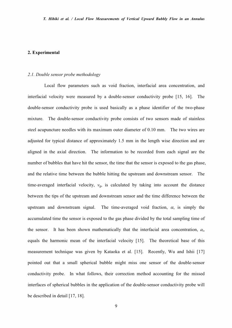
2.1. Double sensor probe methodology
Local flow parameters such as void fraction, interfacial area concentration, and
interfacial velocity were measured by a double-sensor conductivity probe [15, 16]. The
double-sensor conductivity probe is used basically as a phase identifier of the two-phase
mixture. The double-sensor conductivity probe consists of two sensors made of stainless
steel acupuncture needles with its maximum outer diameter of 0.10 mm. The two wires are
adjusted for typical distance of approximately 1.5 mm in the length wise direction and are
aligned in the axial direction. The information to be recorded from each signal are the
number of bubbles that have hit the sensor, the time that the sensor is exposed to the gas phase,
and the relative time between the bubble hitting the upstream and downstream sensor. The
time-averaged interfacial velocity, vg, is calculated by taking into account the distance
between the tips of the upstream and downstream sensor and the time difference between the
upstream and downstream signal. The time-averaged void fraction, α, is simply the
accumulated time the sensor is exposed to the gas phase divided by the total sampling time of
the sensor. It has been shown mathematically that the interfacial area concentration, ai,
equals the harmonic mean of the interfacial velocity [15]. The theoretical base of this
measurement technique was given by Kataoka et al. [15]. Recently, Wu and Ishii [17]
pointed out that a small spherical bubble might miss one sensor of the double-sensor
conductivity probe. In what follows, their correction method accounting for the missed
interfaces of spherical bubbles in the application of the double-sensor conductivity probe will
be described in detail [17, 18].
T. Hibiki et al. / Local Flow Measurements of Vertical Upward Bubbly Flow in an Annulus
10
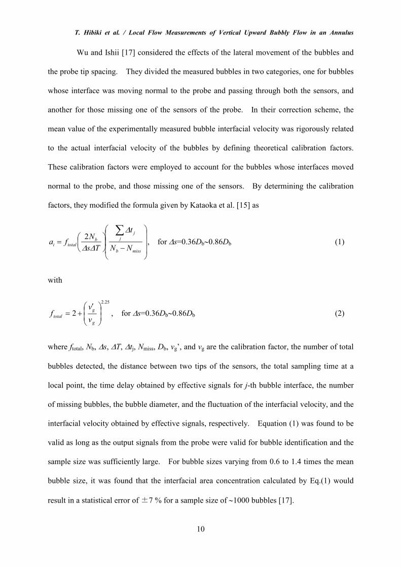
Wu and Ishii [17] considered the effects of the lateral movement of the bubbles and
the probe tip spacing. They divided the measured bubbles in two categories, one for bubbles
whose interface was moving normal to the probe and passing through both the sensors, and
another for those missing one of the sensors of the probe. In their correction scheme, the
mean value of the experimentally measured bubble interfacial velocity was rigorously related
to the actual interfacial velocity of the bubbles by defining theoretical calibration factors.
These calibration factors were employed to account for the bubbles whose interfaces moved
normal to the probe, and those missing one of the sensors. By determining the calibration
factors, they modified the formula given by Kataoka et al. [15] as
−
=∑
missb
j
j
btotali
NN
t
Ts
Nfa
∆
∆∆2
, for ∆s=0.36Db∼0.86Db (1)
with
25.2
2
′+=
g
g
totalv
vf , for ∆s=0.36Db∼0.86Db (2)
where ftotal, Nb, ∆s, ∆T, ∆tj, Nmiss, Db, vg’, and vg are the calibration factor, the number of total
bubbles detected, the distance between two tips of the sensors, the total sampling time at a
local point, the time delay obtained by effective signals for j-th bubble interface, the number
of missing bubbles, the bubble diameter, and the fluctuation of the interfacial velocity, and the
interfacial velocity obtained by effective signals, respectively. Equation (1) was found to be
valid as long as the output signals from the probe were valid for bubble identification and the
sample size was sufficiently large. For bubble sizes varying from 0.6 to 1.4 times the mean
bubble size, it was found that the interfacial area concentration calculated by Eq.(1) would
result in a statistical error of ±7 % for a sample size of ∼1000 bubbles [17].
T. Hibiki et al. / Local Flow Measurements of Vertical Upward Bubbly Flow in an Annulus
11
In the strict sense, the assumption of spherical bubbles may not be valid for any
bubbly flow systems. Bubble shapes in the present experiment may be ellipsoidal with
wobbling interfaces. However, it is considered that the assumption of spherical bubbles
would practically work for the interfacial area concentration measurement on the following
grounds. In the previous study [10], the area-averaged interfacial area concentrations
measured by the double-sensor conductivity probe method were compared with those
measured by a photographic method in relatively low void fraction (<α>≤8 %) and wide
superficial liquid velocity (0.262 m/s ≤<jf>≤3.49 m/s) conditions where the photographic
method could be applied. Here, < > indicates the area-averaged quantity. Good agreement
was obtained between them with an averaged relative deviation of ±6.95 % [11]. In addition
to this, when a spherical bubble is transformed into an ellipsoidal bubble with the aspect ratio
of 2, the resulting increase of the interfacial area is estimated mathematically to be less than
10 % [19].
Using a fast A/D converter Keithly-Metrabyte DAS-1801HC board, local flow
measurements were conducted in a data acquisition program. The acquisition board has a
maximum sampling rate of 333,000 cycles per second. For the data sets measured with the
double-sensor conductivity probe, a minimum of 2000 bubbles were sampled to maintain
similar statistics between the different combinations of gas flow rates. Here, in the void
fraction measurement at bubbly-to-slug flow transition, bubbles can be separated into either a
cap bubble or a small bubble based on the double-sensor conductivity probe signals [12, 20].
The determination whether detected bubbles are cap bubbles is performed based upon the
chord length of bubbles. According to Ishii and Zuber [21], the boundary between distorted
and spherical-cap bubbles is given by 4(σ/g∆ρ)0.5, which corresponds to the bubble diameter
of 10.9 mm in an air-water system at 20 °C. In the present experiment, when local bubble
chord length exceeded this value, bubbles were considered as cap bubbles. Thus, the void
T. Hibiki et al. / Local Flow Measurements of Vertical Upward Bubbly Flow in an Annulus
12
fraction for each category was obtained by the double-sensor conductivity probe separately.
It should be noted here that the signals for cap bubbles were not acquired in the measurement
of the interfacial area concentration, ai,c, as well as the Sauter mean diameter, Dc, but the void
fraction, αc. The Sauter mean diameter in the high void fraction region where cap bubbles
appeared was calculated from DSm=6α/ai≈6α/(ai-ai,c), since the contribution of cap bubbles to
total interfacial area concentration would be relatively small; for example, ai,c/ai=4.76 % for
αc/α=0.2 and Dc/Db=5 [11]. In the present experiment, the number of cap bubbles was not
significant even for high void fraction region. Thus, even Sauter mean diameter might be
able to be approximated by 6(α-αc)/(ai-ai,c). The double-sensor conductivity probe
methodology was detailed in the previous paper [10, 11, 16, 19, 20].
It should be noted here that the double-sensor conductivity probe method may not
work in the vicinity of a wall. The presence of the wall doesn’t allow a bubble to pass the
probe randomly as in the other positions in the channel. This fact will cause a measurement
error in the interfacial area concentration, and interfacial velocity in the vicinity of the wall.
The detailed discussion was given by Kalkach-Navarro [4]. The range where the
double-sensor conductivity probe method can work may roughly be estimated as
Db/DH≤r/(R-R0)≤1-Db/DH, where r, R, R0, and DH are the radial distance measured from the
inner rod surface, the inner radius of the outer round tube, the radius of the inner rod, and the
hydraulic equivalent diameter, respectively. In this experiment (DH=19.1 mm), the effective
range of the double-sensor conductivity probe may roughly be estimated to be
0.10≤r/(R-R0)≤0.90 or 0.16≤r/(R-R0)≤0.84 for Db=2 or 3 mm, respectively. However, the
upstream probe can work well for the measurement of the void fraction and the number of
bubbles which pass the point per unit time. As will be explained later, the local interfacial
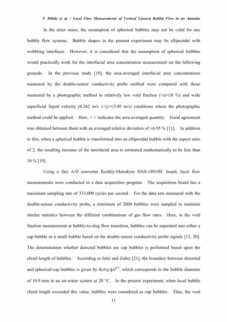
velocities can be fitted by the following function.
T. Hibiki et al. / Local Flow Measurements of Vertical Upward Bubbly Flow in an Annulus
13
( )n
ggRR
RRrv
n
nv
1
0
021
1
−−−
−+
= , (3)
where n is the exponent. For most of bubbly flows [10], the calibration factor, ftotal, can be
approximated to be 2. Therefore, some data of the interfacial area concentration close to the
wall where the double-sensor conductivity probe may not work well were calculated from the
void fraction and the number of bubbles which passed the point per unit time measured by the
front probe, the interfacial velocity estimated by Eq.(3), and Eq.(1).
2.2. Laser Doppler anemometer methodology
Local flow parameters such as liquid velocity, and turbulence intensity were
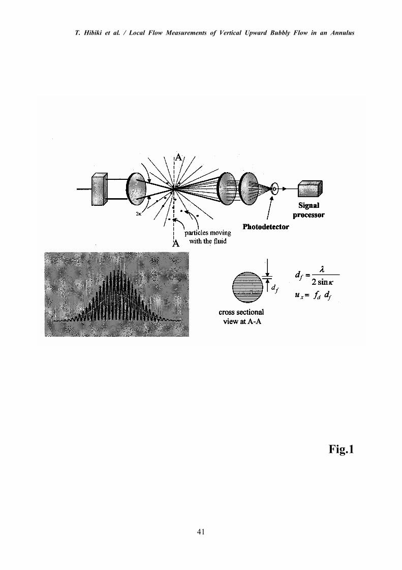
measured by Laser Doppler anemometer (LDA) [22,23]. LDA is one of the most productive
instruments for flow velocity measurements. The dual-beam approach is the most common
optical arrangement used for an LDA system. The intersection of two laser beams from a
common source defines the region from which measurements can be conducted. The actual
measurement region may be a subset of the beam intersection reduced by the field of view of
the receiver optics and the detection limits of the signal processor. Particles crossing the
measurement region scatter light that is collected by a receiver probe. The light signal is
converted to an electrical “Doppler burst” signal with a frequency related to the particle
velocity. The method is shown in Fig.1, where λ, κ, and df are the wavelength of the laser
beam, half of the angle between the dual beams, and the fringe spacing, respectively. The
fluid velocity, ux, is the product of df and the frequency of the proto-detector signal.
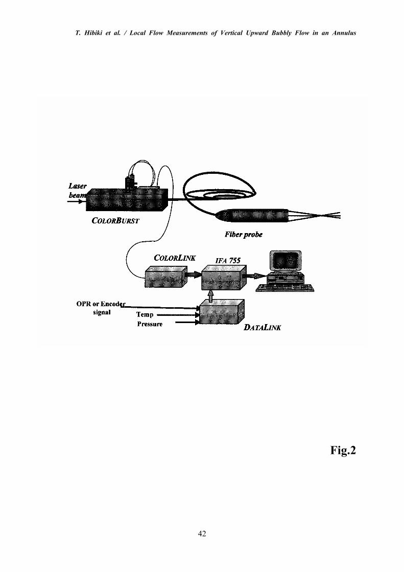
As shown in Fig.2, an integrated LDA system, consisting of an argon-ion laser, a
multicolor beam separator (Model 9201 ColourBurst), a multicolor receiver (Model 9230
ColorLink), a signal processor (IFA 550), a fiberoptic probe (Model 9253-350), a personal
T. Hibiki et al. / Local Flow Measurements of Vertical Upward Bubbly Flow in an Annulus
14
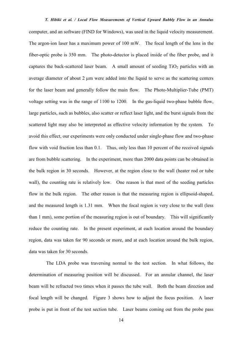
computer, and an software (FIND for Windows), was used in the liquid velocity measurement.
The argon-ion laser has a maximum power of 100 mW. The focal length of the lens in the
fiber-optic probe is 350 mm. The photo-detector is placed inside of the fiber probe, and it
captures the back-scattered laser beam. A small amount of seeding TiO2 particles with an
average diameter of about 2 µm were added into the liquid to serve as the scattering centers
for the laser beam and generally follow the main flow. The Photo-Multiplier-Tube (PMT)
voltage setting was in the range of 1100 to 1200. In the gas-liquid two-phase bubble flow,
large particles, such as bubbles, also scatter or reflect laser light, and the burst signals from the
scattered light may also be interpreted as effective velocity information by the system. To
avoid this effect, our experiments were only conducted under single-phase flow and two-phase
flow with void fraction less than 0.1. Thus, only less than 10 percent of the received signals
are from bubble scattering. In the experiment, more than 2000 data points can be obtained in
the bulk region in 30 seconds. However, at the region close to the wall (heater rod or tube
wall), the counting rate is relatively low. One reason is that most of the seeding particles
flow in the bulk region. The other reason is that the measuring region is ellipsoid-shaped,
and the measured length is 1.31 mm. When the focal region is very close to the wall (less
than 1 mm), some portion of the measuring region is out of boundary. This will significantly
reduce the counting rate. In the present experiment, at each location around the boundary
region, data was taken for 90 seconds or more, and at each location around the bulk region,
data was taken for 30 seconds.
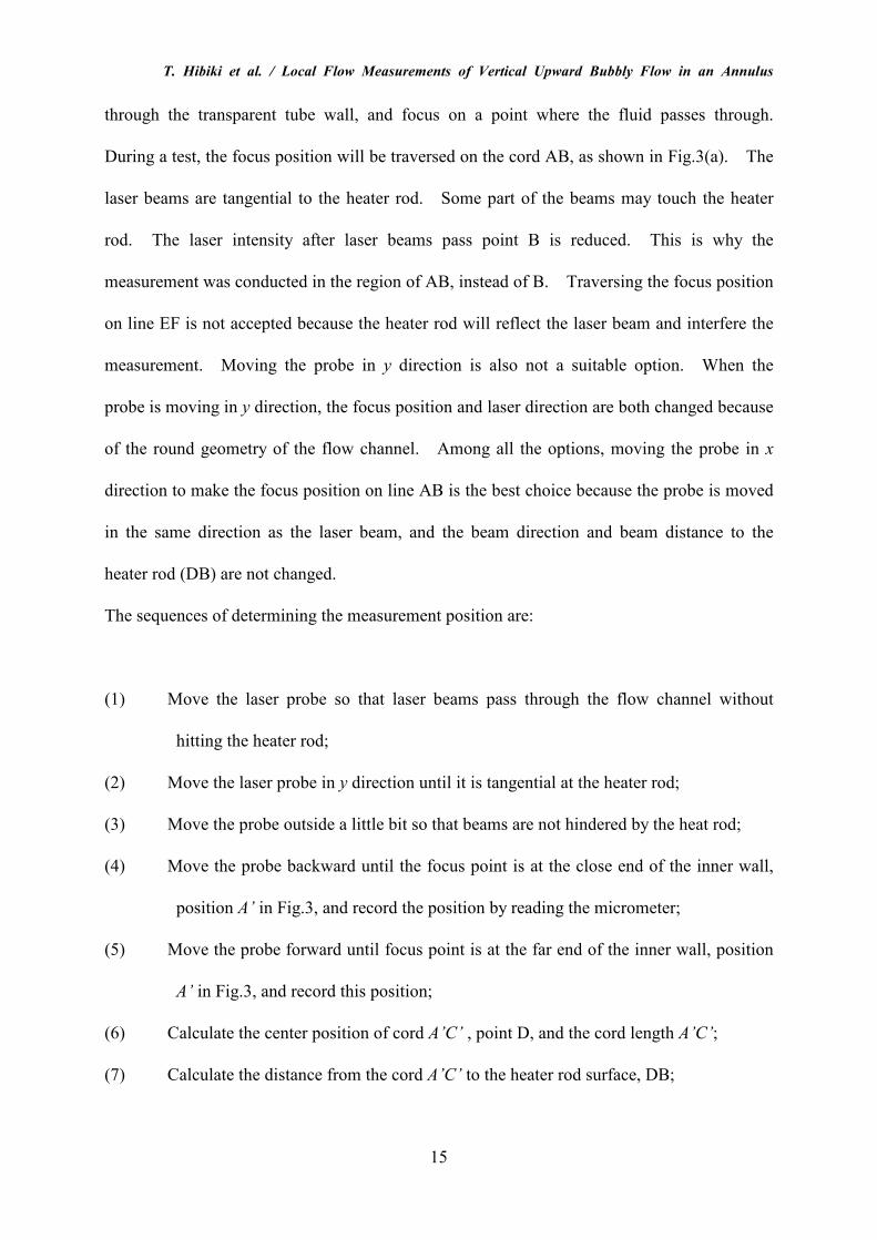
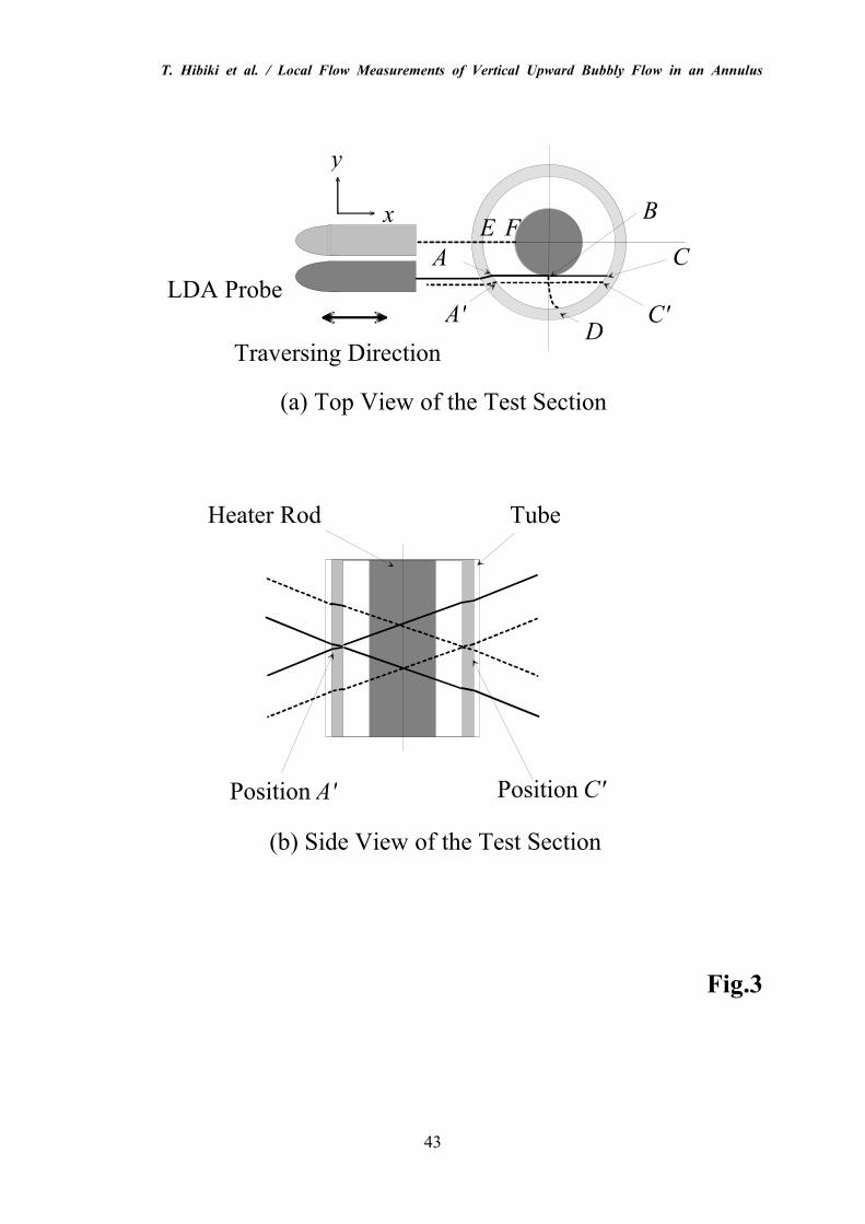
The LDA probe was traversing normal to the test section. In what follows, the
determination of measuring position will be discussed. For an annular channel, the laser
beam will be refracted two times when it passes the tube wall. Both the beam direction and
focal length will be changed. Figure 3 shows how to adjust the focus position. A laser
probe is put in front of the test section tube. Laser beams coming out from the probe pass
T. Hibiki et al. / Local Flow Measurements of Vertical Upward Bubbly Flow in an Annulus
15
through the transparent tube wall, and focus on a point where the fluid passes through.
During a test, the focus position will be traversed on the cord AB, as shown in Fig.3(a). The
laser beams are tangential to the heater rod. Some part of the beams may touch the heater
rod. The laser intensity after laser beams pass point B is reduced. This is why the
measurement was conducted in the region of AB, instead of B. Traversing the focus position
on line EF is not accepted because the heater rod will reflect the laser beam and interfere the
measurement. Moving the probe in y direction is also not a suitable option. When the
probe is moving in y direction, the focus position and laser direction are both changed because
of the round geometry of the flow channel. Among all the options, moving the probe in x
direction to make the focus position on line AB is the best choice because the probe is moved
in the same direction as the laser beam, and the beam direction and beam distance to the
heater rod (DB) are not changed.
The sequences of determining the measurement position are:
(1) Move the laser probe so that laser beams pass through the flow channel without
hitting the heater rod;
(2) Move the laser probe in y direction until it is tangential at the heater rod;
(3) Move the probe outside a little bit so that beams are not hindered by the heat rod;
(4) Move the probe backward until the focus point is at the close end of the inner wall,
position A’ in Fig.3, and record the position by reading the micrometer;
(5) Move the probe forward until focus point is at the far end of the inner wall, position
A’ in Fig.3, and record this position;
(6) Calculate the center position of cord A’C’ , point D, and the cord length A’C’;
(7) Calculate the distance from the cord A’C’ to the heater rod surface, DB;
T. Hibiki et al. / Local Flow Measurements of Vertical Upward Bubbly Flow in an Annulus
16
(8) Move the probe in y direction toward the heat rod with the distance of DB so that the
beams are tangential to the heater rod at point B;
(9) Calculate the cord length AC;
(10) Calculate the positions of the probe corresponding to the certain non-dimensional
radius of focus points. It should be noted here that because the refractive index
difference between water and air, the actual location change of measurement
volume, ∆r, is not same as the probe traversing distance ∆d. The refractive index
of water and the polycarbonate tube are 1.33 and 1.66, respectively.
During the test, a very small angle between the direction of the probe and the traverse
system were found. In order to deal with this problem, first, the probe was moved backward
or forward to find the actual locations of heater boundary and tube boundary by checking the
LDA signal. Second, assuming that the focus position is traversing on the line between these
two boundaries, the angle between beam and traverse direction was calculated, and the real
non-dimensional radius was also calculated. The LDA methodology was detailed in the
previous paper [22,23].
2.3. Two-phase flow experiment
An experimental facility was designed to measure the relevant two-phase parameters
necessary for developing constitutive models for the two-fluid model in subcooled boiling.
It was scaled to a prototypic BWR based on scaling criteria for geometric, hydrodynamic, and
thermal similarities [14]. The experimental facility, instrumentation, and data acquisition
system are briefly described in this section [14].
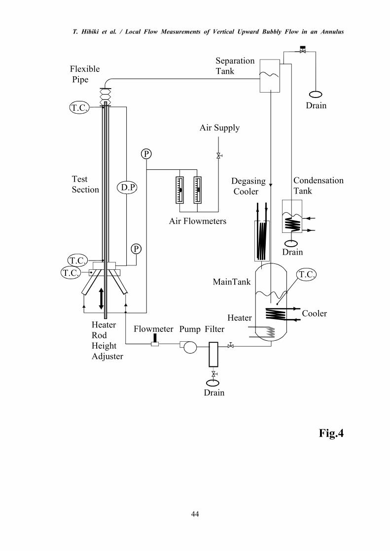
The two-phase flow experiment was performed by using a flow loop constructed at
Thermal-Hydraulics and Reactor Safety Laboratory in Purdue University. Figure 4 shows
T. Hibiki et al. / Local Flow Measurements of Vertical Upward Bubbly Flow in an Annulus
17
the experimental facility layout. The water supply is held in the holding tank. The tank is
open to the atmosphere through a heat exchanger mounted to the top to prevent explosion or
collapse and to degas from the water. There is a cartridge heater inside the tank to heat the
water and maintain the inlet water temperature. A cooling line runs inside the tank to
provide control of the inlet water temperature and post-experimental cooling of the tank.
Water is pumped with a positive displacement, eccentric screw pump, capable of providing a
constant head with minimum pressure oscillation. The water, which flows through a
magnetic flow meter, is divided into four separate flows and can then be mixed with air before
it is injected into the test section to study adiabatic air-water bubbly flow. For the adiabatic
air-water flow experiment, porous spargers with the pore size of 10 µm are used as air
injectors. The test section is an annular geometry that is formed by a clear polycarbonate
tube on the outside and a cartridge heater on the inside. The test section is 38.1 mm inner
diameter and has a 3.18 mm wall thickness. The overall length of the heater is 2670 mm and
has a 19.1 mm outer diameter. The heated section of the heater rod is 1730 mm long. The
maximum power of the heater is 20 kW and has a maximum surface heat flux of 0.193
MW/m2. The heater rod has one thermocouple that is connected to the process controller to
provide feedback control. The heater rod can be traversed vertically to allow many axial
locations to be studied with four instrument ports attached to the test section. At each port
there is an electrical conductivity probe. A pressure tap and thermocouple are placed at the
inlet and exit of the test section. A differential pressure cell is connected between the inlet
and outlet pressure taps. The loop can also be operated with a diabatic steam-water flow in a
future study. The two-phase mixture flows out of the test section to a separator tank and the
gas phase is piped away and the water is returned to the holding tank.
The flow rates of the air and water were measured with a rotameter and a magnetic
flow meter, respectively. The loop temperature was kept at a constant temperature (20 °C)
T. Hibiki et al. / Local Flow Measurements of Vertical Upward Bubbly Flow in an Annulus
18
within the deviation of ±0.2 °C by a heat exchanger installed in a water reservoir. The local
flow measurements using the LDA were performed at an axial location of z/DH=49.8 and
thirteen radial locations from r/(R-R0)=0.025 to 0.975. The local flow measurements using
the double-sensor conductivity probe were performed at two axial locations of z/DH=40.3 and
61.7 and ten radial locations from r/(R-R0)=0.05 to 0.9. To compare the gas flow
measurements with the liquid flow measurements, flow parameters for the gas phase
measured at z/DH=40.3 and 61.7 were averaged to estimate those at z/DH=51.0, where was
very close to the axial position for liquid flow measurements (z/DH=49.8). A γ–densitometer
was installed at z/DH=51.1 in the loop to measure the area-averaged void fraction. The flow
conditions in this experiment are tabulated in Table 1. The area-averaged superficial gas
velocities in this experiment were roughly determined so as to provide the same area-averaged
void fractions among different conditions of superficial liquid velocity, namely <α>=0.050,
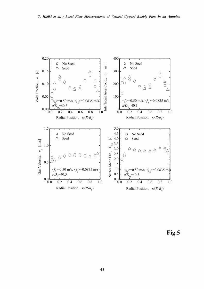
0.10, 0.15, 0.20, and 0.25. As explained in section 2.2, a small amount of seeding TiO2
particles with an average diameter of about 2 µm were added into the liquid to serve as the
scattering centers for the laser beam. However, as shown in Fig.5, the seeding particles did
not affect the local flow measurements.
In order to verify the accuracy of local measurements, the area-averaged quantities
obtained by integrating the local flow parameters over the flow channel were compared with
those measured by other cross-calibration methods such as a γ-densitometer for void fraction,
a photographic method for interfacial area concentration, a rotameter for superficial gas
velocity, and a magnetic flow meter for superficial liquid velocity. Area-averaged superficial
gas velocity was obtained from local void fraction and gas velocity measured by the
double-sensor conductivity probe, whereas area-averaged superficial liquid velocity was
obtained from local void fraction measured by the double-sensor conductivity probe and local
liquid velocity measured by the LDA. Good agreements were obtained between the
T. Hibiki et al. / Local Flow Measurements of Vertical Upward Bubbly Flow in an Annulus
19
area-averaged void fraction, interfacial area concentration, superficial gas velocity, and
superficial liquid velocity obtained from the local measurements and those measured by the
γ-densitometer, the photographic method, the rotameter, and the magnetic flow meter with
averaged relative deviations of ±12.8 [24], ±6.95 [11], ±12.9 %, and ±15.5 %,
respectively.
3. Results and discussion
3.1. Local flow parameters
3.1.1. Local flow parameters in gas phase
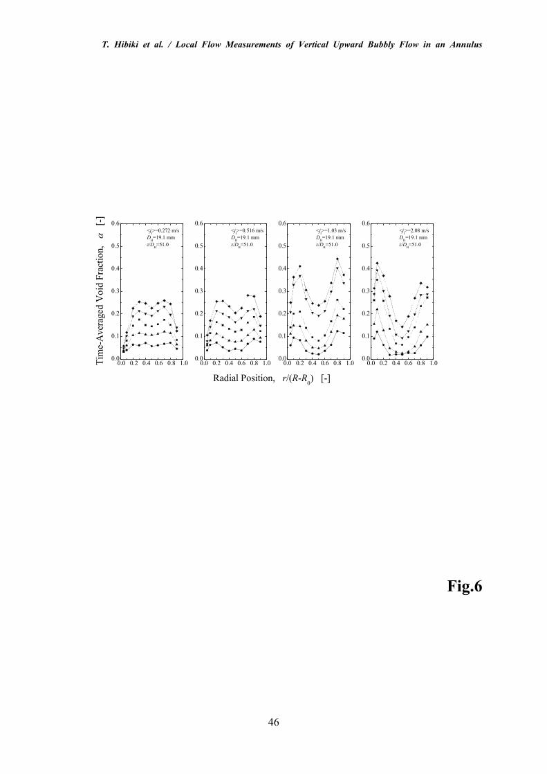
Figures 6, 7, 8, and 9 show the behavior of void fraction, interfacial area
concentration, interfacial velocity, and Sauter mean diameter profiles measured in this
experiment. The meanings of the symbols in these figures are found in Table 1. As can be
seen from Fig.6, various phase distribution patterns similar to those in round tubes were
observed in the present experiment, and void fraction profiles were found to be almost
symmetrical with respect to the channel center, r/(R-R0)=0.5. Serizawa and Kataoka
classified the phase distribution pattern into four basic types of the distributions, that is, “wall
peak”, “intermediate peak”, “core peak”, and “transition” [1]. The wall peak is characterized
as sharp peak with relatively high void fraction near the channel wall and plateau with very
low void fraction around the channel center. The intermediate peak is explained as broad
peak in void fraction near the channel wall and plateau with medium void fraction around the
channel center. The core peak is defined as broad peak around the channel center and no
peak near the channel wall. The transition is described as two broad peaks around the
channel wall and center. In Fig.10, non-dimensional peak void fraction (upper figures) and
T. Hibiki et al. / Local Flow Measurements of Vertical Upward Bubbly Flow in an Annulus
20
peak radial position (lower figures) are plotted against the area-averaged void fraction as a
parameter of the superficial liquid velocity. The non-dimensional void fraction at the peak is
defined as (αP-αC)/αP, where αP and αC are the void fraction at the peak and the channel
center, respectively. (αP-αC)/αP=0 and 1 indicate no wall peak and very sharp wall peak,
respectively. The non-dimensional radial position at the peak is defined as rP/(R-R0), where
rP is the peak radial position. The left and right figures are the data measured for peaks
appeared at inner and outer sides of the channel, respectively.
As the superficial liquid velocity increased, the radial position at the void fraction
peak was moved towards the channel wall. The increase in the superficial liquid velocity
also augmented the void fraction at the peak and made the void fraction peak sharp. On the
other hand, in the present experimental condition, the increase in the void fraction did not
change the radial position at the void fraction peak significantly, and decreased the
non-dimensional void fraction at the peak, resulting in the broad void fraction peak. As
general trends observed in the present experiment, the increase in the superficial liquid
velocity decreased the bubble size, whereas the increase in the void fraction increased the
bubble size. It was pointed out that the bubble size and liquid velocity profile would affect
the void fraction distribution. Similar phenomena were also observed by Sekoguchi et al.
[25], Zun [26], and Serizawa and Kataoka [1]. Sekoguchi et al. [25] observed the behaviors
of isolated bubbles, which were introduced into vertical water flow in a 25 mm × 50 mm
rectangular channel through a single nozzle. Based on their observations, they found that the
bubble behaviors in dilute suspension flow might depend on the bubble size and the bubble
shape. In their experiment, only distorted ellipsoidal bubbles with a diameter smaller than
nearly 5 mm tended to migrate toward the wall, whereas distorted ellipsoidal bubbles with a
diameter larger than 5 mm and spherical bubbles rose in the channel center. On the other
hand, for the water velocity lower than 0.3 m/s, no bubbles were observed in the wall region.
T. Hibiki et al. / Local Flow Measurements of Vertical Upward Bubbly Flow in an Annulus
21
Zun [26] also obtained a similar result. Zun performed an experiment to study void fraction
radial profiles in upward vertical bubbly flow at very low average void fractions, around
0.5 %. In his experiment, the wall void peaking flow regime existed both in laminar and
turbulent bulk liquid flow. The experimental results on turbulent bulk liquid flow at
Reynolds number near 1000 showed distinctive higher bubble concentration at the wall region
if the bubble equivalent sphere diameter appeared in the range of 0.8 and 3.6 mm.
Intermediate void profiles were observed at bubble sizes either between 0.6 and 0.8 mm or 3.6
and 5.1 mm. Bubbles smaller than 0.6 mm or larger than 5.1 mm tended to migrate towards
at the channel center. Thus, these experimental results suggested that the bubble size would
play a dominant role in void fraction profiles. Serizawa and Kataoka [1] also gave an
extensive review on the bubble behaviors in bubbly-flow regime.
Figure 11 shows a map of phase distribution patterns observed in this experiment.
The open symbols of circle, triangle, and square in Fig.11 indicate the wall peak, the
intermediate peak, and the core peak, respectively. The transition was not observed in this
experiment. Since Serizawa and Kataoka [1] did not give the quantitative definitions of the
wall and intermediate peaks, the classification between the wall and intermediate peaks in the
present study were performed as the wall peak for (αP-αC)/αP≥0.5 and the intermediate peak
for (αP-αC)/αP<0.5. For <jf>=0.272 m/s and void fraction lower than 0.10, the void fraction
profiles were almost uniform along the channel radius with some decrease in size near the
wall, and such void fraction profiles were categorized as the core peak in this experiment.
The solid and broken lines in Fig.11 are, respectively, the flow regime transition boundaries
predicted by the model of Taitel et al. [27] and the phase distribution pattern transition
boundaries, which were developed by Serizawa and Kataoka [1] based on experiments
performed by different researchers with different types of bubble injections in round tubes (20
mm ≤ D ≤ 86.4 mm). A fairly good agreement was obtained between the
T. Hibiki et al. / Local Flow Measurements of Vertical Upward Bubbly Flow in an Annulus
22
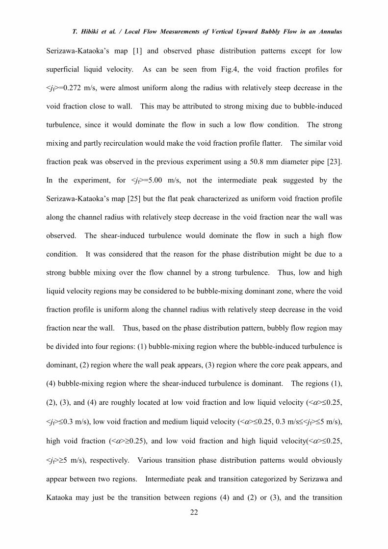
Serizawa-Kataoka’s map [1] and observed phase distribution patterns except for low
superficial liquid velocity. As can be seen from Fig.4, the void fraction profiles for
<jf>=0.272 m/s, were almost uniform along the radius with relatively steep decrease in the
void fraction close to wall. This may be attributed to strong mixing due to bubble-induced
turbulence, since it would dominate the flow in such a low flow condition. The strong
mixing and partly recirculation would make the void fraction profile flatter. The similar void
fraction peak was observed in the previous experiment using a 50.8 mm diameter pipe [23].
In the experiment, for <jf>=5.00 m/s, not the intermediate peak suggested by the
Serizawa-Kataoka’s map [25] but the flat peak characterized as uniform void fraction profile
along the channel radius with relatively steep decrease in the void fraction near the wall was
observed. The shear-induced turbulence would dominate the flow in such a high flow
condition. It was considered that the reason for the phase distribution might be due to a
strong bubble mixing over the flow channel by a strong turbulence. Thus, low and high
liquid velocity regions may be considered to be bubble-mixing dominant zone, where the void
fraction profile is uniform along the channel radius with relatively steep decrease in the void
fraction near the wall. Thus, based on the phase distribution pattern, bubbly flow region may
be divided into four regions: (1) bubble-mixing region where the bubble-induced turbulence is
dominant, (2) region where the wall peak appears, (3) region where the core peak appears, and
(4) bubble-mixing region where the shear-induced turbulence is dominant. The regions (1),
(2), (3), and (4) are roughly located at low void fraction and low liquid velocity (<α>≤0.25,
<jf>≤0.3 m/s), low void fraction and medium liquid velocity (<α>≤0.25, 0.3 m/s≤<jf>≤5 m/s),
high void fraction (<α>≥0.25), and low void fraction and high liquid velocity(<α>≤0.25,
<jf>≥5 m/s), respectively. Various transition phase distribution patterns would obviously
appear between two regions. Intermediate peak and transition categorized by Serizawa and
Kataoka may just be the transition between regions (4) and (2) or (3), and the transition
T. Hibiki et al. / Local Flow Measurements of Vertical Upward Bubbly Flow in an Annulus
23
between regions (1) and (2) or (3), respectively.
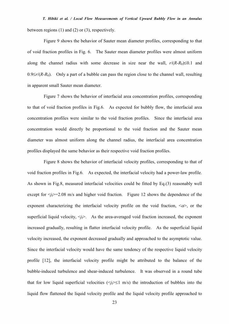
Figure 9 shows the behavior of Sauter mean diameter profiles, corresponding to that
of void fraction profiles in Fig. 6. The Sauter mean diameter profiles were almost uniform
along the channel radius with some decrease in size near the wall, r/(R-R0)≤0.1 and
0.9≤r/(R-R0). Only a part of a bubble can pass the region close to the channel wall, resulting
in apparent small Sauter mean diameter.
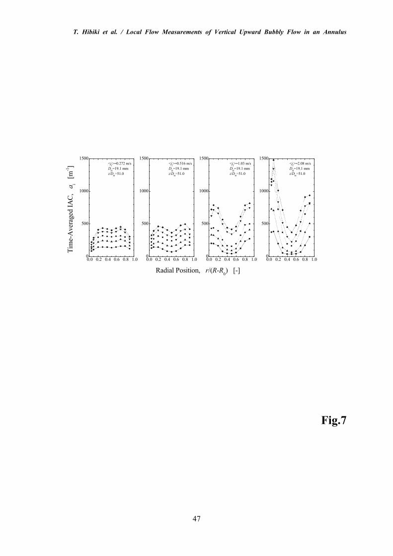
Figure 7 shows the behavior of interfacial area concentration profiles, corresponding
to that of void fraction profiles in Fig.6. As expected for bubbly flow, the interfacial area
concentration profiles were similar to the void fraction profiles. Since the interfacial area
concentration would directly be proportional to the void fraction and the Sauter mean
diameter was almost uniform along the channel radius, the interfacial area concentration
profiles displayed the same behavior as their respective void fraction profiles.
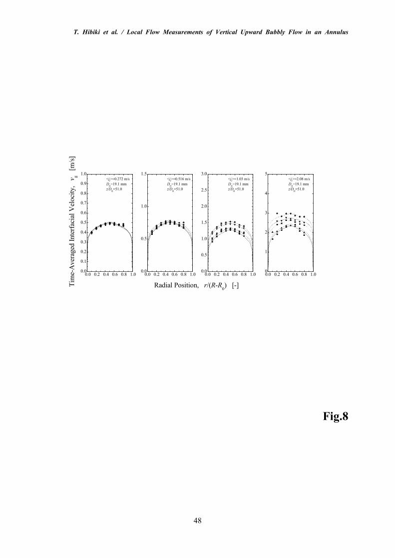
Figure 8 shows the behavior of interfacial velocity profiles, corresponding to that of
void fraction profiles in Fig.6. As expected, the interfacial velocity had a power-law profile.
As shown in Fig.8, measured interfacial velocities could be fitted by Eq.(3) reasonably well
except for <jf>=2.08 m/s and higher void fraction. Figure 12 shows the dependence of the
exponent characterizing the interfacial velocity profile on the void fraction, <α>, or the
superficial liquid velocity, <jf>. As the area-averaged void fraction increased, the exponent
increased gradually, resulting in flatter interfacial velocity profile. As the superficial liquid
velocity increased, the exponent decreased gradually and approached to the asymptotic value.
Since the interfacial velocity would have the same tendency of the respective liquid velocity
profile [12], the interfacial velocity profile might be attributed to the balance of the
bubble-induced turbulence and shear-induced turbulence. It was observed in a round tube
that for low liquid superficial velocities (<jf>≤1 m/s) the introduction of bubbles into the
liquid flow flattened the liquid velocity profile and the liquid velocity profile approached to
T. Hibiki et al. / Local Flow Measurements of Vertical Upward Bubbly Flow in an Annulus
24
that of developed single-phase flow with the increase of void fraction [12]. It was also
reported that the effect of the bubble introduction into the liquid on the liquid velocity profile
was diminishing with increasing gas and liquid velocities and for high liquid velocities
(<jf>≥1 m/s) the liquid velocity profile came to be the power law profile as the flow developed.
Thus, for low or high liquid velocity, the bubble-induced or shear-induced turbulence would
play an important role in determining the liquid velocity profile, respectively.
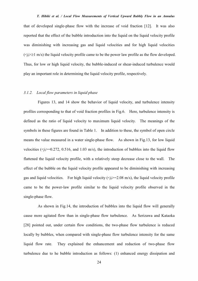
3.1.2. Local flow parameters in liquid phase
Figures 13, and 14 show the behavior of liquid velocity, and turbulence intensity
profiles corresponding to that of void fraction profiles in Fig.6. Here, turbulence intensity is
defined as the ratio of liquid velocity to maximum liquid velocity. The meanings of the
symbols in these figures are found in Table 1. In addition to these, the symbol of open circle
means the value measured in a water single-phase flow. As shown in Fig.13, for low liquid
velocities (<jf>=0.272, 0.516, and 1.03 m/s), the introduction of bubbles into the liquid flow
flattened the liquid velocity profile, with a relatively steep decrease close to the wall. The
effect of the bubble on the liquid velocity profile appeared to be diminishing with increasing
gas and liquid velocities. For high liquid velocity (<jf>=2.08 m/s), the liquid velocity profile
came to be the power-law profile similar to the liquid velocity profile observed in the
single-phase flow.
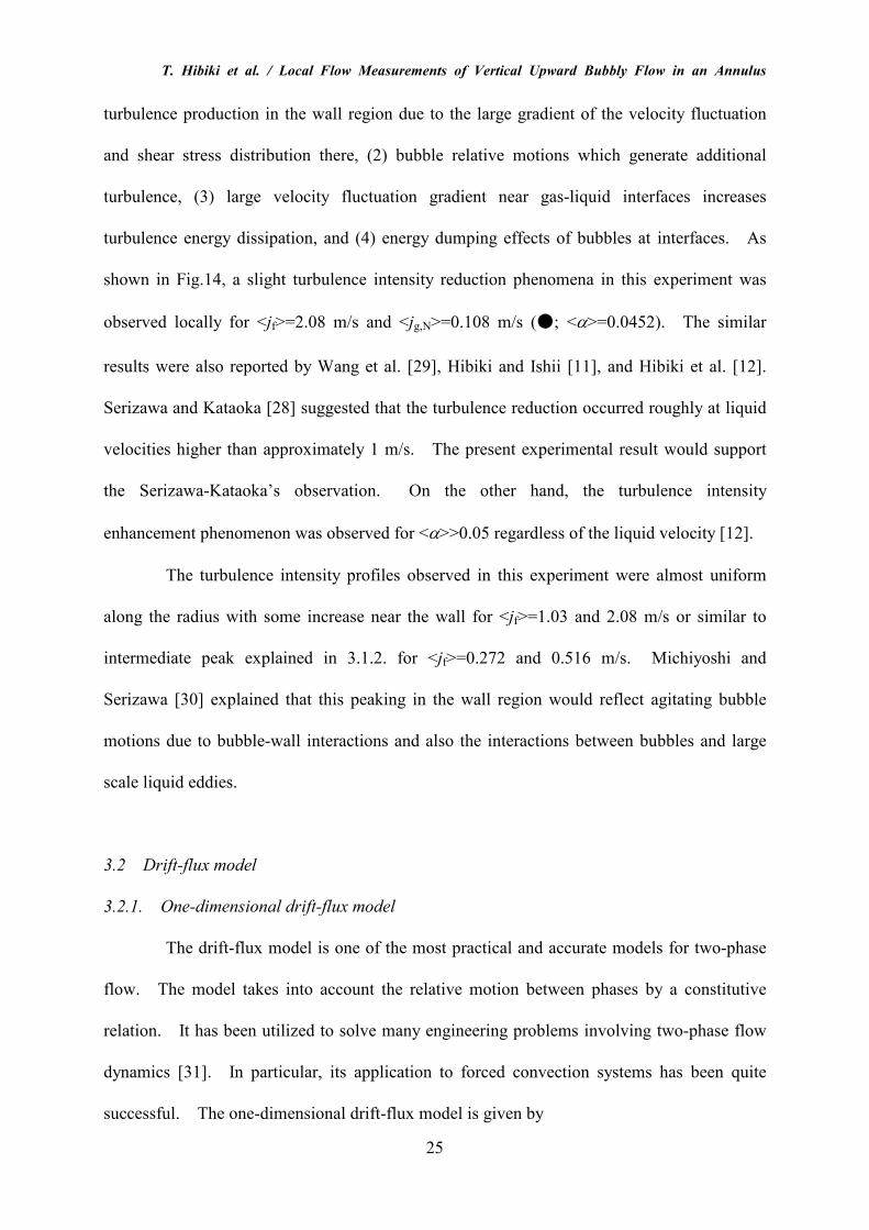
As shown in Fig.14, the introduction of bubbles into the liquid flow will generally
cause more agitated flow than in single-phase flow turbulence. As Serizawa and Kataoka
[28] pointed out, under certain flow conditions, the two-phase flow turbulence is reduced
locally by bubbles, when compared with single-phase flow turbulence intensity for the same
liquid flow rate. They explained the enhancement and reduction of two-phase flow
turbulence due to he bubble introduction as follows: (1) enhanced energy dissipation and
T. Hibiki et al. / Local Flow Measurements of Vertical Upward Bubbly Flow in an Annulus
25
turbulence production in the wall region due to the large gradient of the velocity fluctuation
and shear stress distribution there, (2) bubble relative motions which generate additional
turbulence, (3) large velocity fluctuation gradient near gas-liquid interfaces increases
turbulence energy dissipation, and (4) energy dumping effects of bubbles at interfaces. As
shown in Fig.14, a slight turbulence intensity reduction phenomena in this experiment was
observed locally for <jf>=2.08 m/s and <jg,N>=0.108 m/s (●; <α>=0.0452). The similar
results were also reported by Wang et al. [29], Hibiki and Ishii [11], and Hibiki et al. [12].
Serizawa and Kataoka [28] suggested that the turbulence reduction occurred roughly at liquid
velocities higher than approximately 1 m/s. The present experimental result would support
the Serizawa-Kataoka’s observation. On the other hand, the turbulence intensity
enhancement phenomenon was observed for <α>>0.05 regardless of the liquid velocity [12].
The turbulence intensity profiles observed in this experiment were almost uniform
along the radius with some increase near the wall for <jf>=1.03 and 2.08 m/s or similar to
intermediate peak explained in 3.1.2. for <jf>=0.272 and 0.516 m/s. Michiyoshi and
Serizawa [30] explained that this peaking in the wall region would reflect agitating bubble
motions due to bubble-wall interactions and also the interactions between bubbles and large
scale liquid eddies.
3.2 Drift-flux model
3.2.1. One-dimensional drift-flux model
The drift-flux model is one of the most practical and accurate models for two-phase
flow. The model takes into account the relative motion between phases by a constitutive
relation. It has been utilized to solve many engineering problems involving two-phase flow
dynamics [31]. In particular, its application to forced convection systems has been quite
successful. The one-dimensional drift-flux model is given by
T. Hibiki et al. / Local Flow Measurements of Vertical Upward Bubbly Flow in an Annulus
26
gj
gjg
g VjCv
jj
jjv +=+== 0α
α
αα
α, (4)
where vgj, C0 and Vgj are the drift velocity of a gas phase defined as the velocity of the gas
phase with respect to the volume center to the mixture, j, the distribution parameter defined by
Eq.(5) and the void-fraction-weighted mean drift velocity defined by Eq.(6), respectively.
<< >> means the void-fraction-weighted mean value.
j
jC
αα
≡0 , (5)
and
α
α gj
gj
vV = . (6)
The void-fraction-weighted mean gas velocity, <jg>/<α>, and the cross-sectional mean
mixture volumetric flux, <j>, are easily obtainable parameters in experiments. Therefore,
Eq.(4) suggests a plot of <jg>/<α> versus <j>. An important characteristic of such a plot is
that, for two-phase flow regimes with fully-developed void and velocity profiles, the data
points cluster around a straight line. The value of the distribution parameter, C0, has been
obtained indirectly from the slope of the line, whereas the intercept of this line with the
void-fraction-weighted mean gas velocity axis can be interpreted as the
void-fraction-weighted mean local drift velocity, Vgj. As recent development of local sensor
techniques enables the measurement of the local flow parameters in a bubbly flow such as
void fraction, and gas and liquid velocities, the values of C0 and Vgj in a bubbly flow can be
determined directly by Eqs.(5) and (6) from experimental data of the local flow parameters.
3.2.2. Constitutive equation of distribution parameter
Ishii [31] developed a simple correlation for the distribution parameter in

T. Hibiki et al. / Local Flow Measurements of Vertical Upward Bubbly Flow in an Annulus
27
bubbly-flow regime. Ishii first considered a fully-developed bubbly flow and assumed that
C0 would depend on the density ratio, ρg/ρf, and on the Reynolds number, Re. As the density
ratio approaches the unity, the distribution parameter, C0, should become unity. Based on
the limit and various experimental data in fully-developed flows, the distribution parameter
was given approximately by
( ) ( ){ } fgReCReCC ρρ10 −−= ∞∞ , (7)
where C∞ is the asymptotic value of C0. Here, the density group scales the inertia effects of
each phase in a transverse void distribution. Physically, Eq.(7) models the tendency of the
lighter phase to migrate into a higher-velocity region, thus resulting in a higher void
concentration in the central region [31]. For a laminar flow, C∞ is 2, but due to the large
velocity gradient, C0 is very sensitive to <α> at low void fractions [31].
Based on a wide range of Reynolds number, Ishii [31] approximated C∞ to be 1.2 for
a flow in a round tube [31]. Thus, for a fully-developed turbulent bubbly flow in a round
tube,
fgC ρρ2.02.10 −≅ . (8)
Recently, Hibiki and Ishii [32] suggested that the constitutive equation for the
distribution parameter given by Eq.(8) might not give a good prediction in the bubbly-flow
regime. Wall peaking in void fraction distribution tends to decrease the distribution
parameter considerably. In the mid-1970s, very few databases on local flow parameters were
available and, therefore, it might be very difficult to include such local phenomena in the final
constitutive equation. As local flow measurement techniques such as double-sensor
conductivity probe method and hotfilm anemometry have been developed, databases of local
flow parameters for gas and liquid phases in the bubbly flow have been developed extensively.
T. Hibiki et al. / Local Flow Measurements of Vertical Upward Bubbly Flow in an Annulus
28
This enabled reassessment of the constitutive equations for the distribution parameter and the
drift velocity by using the local flow parameters such as void fraction, gas velocity, and liquid
velocity. Hibiki and Ishii [32] modified the constitutive equation for the distribution
parameter, Eq.(8), based on bubble migration dynamics in a flow field. Detailed discussion
on the bubbly dynamics suggested that a key parameter determining the phase distribution
pattern would be a bubble diameter, and Hibiki and Ishii [32] proposed the following simple
correlation as:
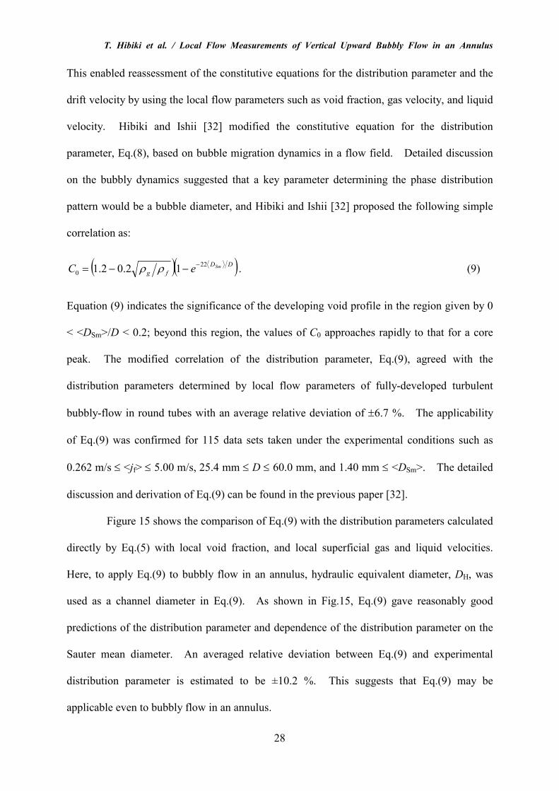
( )( )DD
fgSmeC
22
0 12.02.1−−−= ρρ . (9)
Equation (9) indicates the significance of the developing void profile in the region given by 0
< <DSm>/D < 0.2; beyond this region, the values of C0 approaches rapidly to that for a core
peak. The modified correlation of the distribution parameter, Eq.(9), agreed with the
distribution parameters determined by local flow parameters of fully-developed turbulent
bubbly-flow in round tubes with an average relative deviation of ±6.7 %. The applicability
of Eq.(9) was confirmed for 115 data sets taken under the experimental conditions such as
0.262 m/s ≤ <jf> ≤ 5.00 m/s, 25.4 mm ≤ D ≤ 60.0 mm, and 1.40 mm ≤ <DSm>. The detailed
discussion and derivation of Eq.(9) can be found in the previous paper [32].
Figure 15 shows the comparison of Eq.(9) with the distribution parameters calculated
directly by Eq.(5) with local void fraction, and local superficial gas and liquid velocities.
Here, to apply Eq.(9) to bubbly flow in an annulus, hydraulic equivalent diameter, DH, was
used as a channel diameter in Eq.(9). As shown in Fig.15, Eq.(9) gave reasonably good
predictions of the distribution parameter and dependence of the distribution parameter on the
Sauter mean diameter. An averaged relative deviation between Eq.(9) and experimental
distribution parameter is estimated to be ±10.2 %. This suggests that Eq.(9) may be
applicable even to bubbly flow in an annulus.
T. Hibiki et al. / Local Flow Measurements of Vertical Upward Bubbly Flow in an Annulus
29
For a practical use, the Sauter mean diameter in Eq.(9) should be correlated with
easily measurable quantities such as superficial gas and liquid velocities. Recently, Hibiki
and Ishii [33] developed new correlation of the interfacial area concentration under steady
fully-developed bubbly flow conditions based on the interfacial area transport equation as
follows:
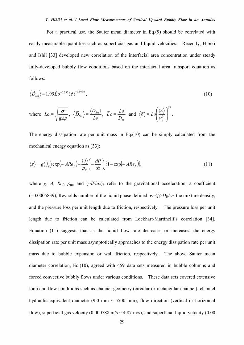
0796.0335.0 ~~99.1
~ −−= εoLDSm , (10)
where ρ∆
σg
Lo ≡ , Lo
DD Sm
Sm ≡~
, HD
LooL ≡
~ and
41
3
~
≡
f
Loν
εε .
The energy dissipation rate per unit mass in Eq.(10) can be simply calculated from the
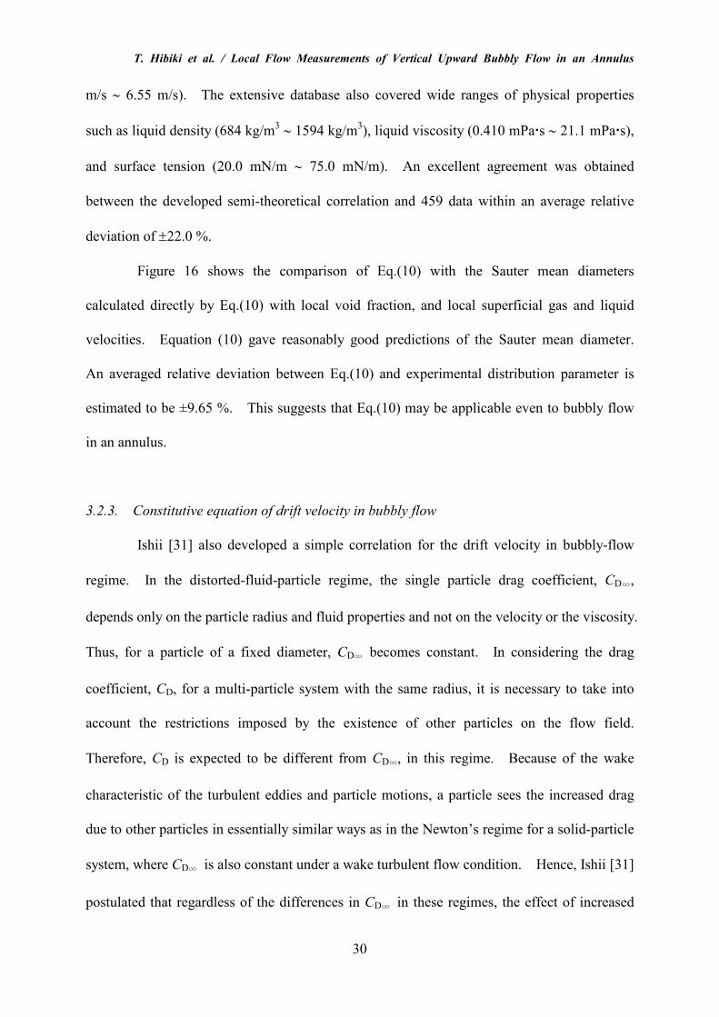
mechanical energy equation as [33]:
( ) ( ){ }f
Fm
fg ARedz
dPjARejg −−
−+−= exp1expρ
ε , (11)
where g, A, Ref, ρm, and (-dP/dz)F refer to the gravitational acceleration, a coefficient
(=0.0005839), Reynolds number of the liquid phase defined by <jf>DH/νf, the mixture density,
and the pressure loss per unit length due to friction, respectively. The pressure loss per unit
length due to friction can be calculated from Lockhart-Martinelli’s correlation [34].
Equation (11) suggests that as the liquid flow rate decreases or increases, the energy
dissipation rate per unit mass asymptotically approaches to the energy dissipation rate per unit
mass due to bubble expansion or wall friction, respectively. The above Sauter mean
diameter correlation, Eq.(10), agreed with 459 data sets measured in bubble columns and
forced convective bubbly flows under various conditions. These data sets covered extensive
loop and flow conditions such as channel geometry (circular or rectangular channel), channel
hydraulic equivalent diameter (9.0 mm ∼ 5500 mm), flow direction (vertical or horizontal
flow), superficial gas velocity (0.000788 m/s ∼ 4.87 m/s), and superficial liquid velocity (0.00
T. Hibiki et al. / Local Flow Measurements of Vertical Upward Bubbly Flow in an Annulus
30
m/s ∼ 6.55 m/s). The extensive database also covered wide ranges of physical properties
such as liquid density (684 kg/m3 ∼ 1594 kg/m3
), liquid viscosity (0.410 mPa�s ∼ 21.1 mPa�s),
and surface tension (20.0 mN/m ∼ 75.0 mN/m). An excellent agreement was obtained
between the developed semi-theoretical correlation and 459 data within an average relative
deviation of ±22.0 %.
Figure 16 shows the comparison of Eq.(10) with the Sauter mean diameters
calculated directly by Eq.(10) with local void fraction, and local superficial gas and liquid
velocities. Equation (10) gave reasonably good predictions of the Sauter mean diameter.
An averaged relative deviation between Eq.(10) and experimental distribution parameter is
estimated to be ±9.65 %. This suggests that Eq.(10) may be applicable even to bubbly flow
in an annulus.
3.2.3. Constitutive equation of drift velocity in bubbly flow
Ishii [31] also developed a simple correlation for the drift velocity in bubbly-flow
regime. In the distorted-fluid-particle regime, the single particle drag coefficient, CD∞,
depends only on the particle radius and fluid properties and not on the velocity or the viscosity.
Thus, for a particle of a fixed diameter, CD∞ becomes constant. In considering the drag
coefficient, CD, for a multi-particle system with the same radius, it is necessary to take into
account the restrictions imposed by the existence of other particles on the flow field.
Therefore, CD is expected to be different from CD∞, in this regime. Because of the wake
characteristic of the turbulent eddies and particle motions, a particle sees the increased drag
due to other particles in essentially similar ways as in the Newton’s regime for a solid-particle
system, where CD∞ is also constant under a wake turbulent flow condition. Hence, Ishii [31]
postulated that regardless of the differences in CD∞ in these regimes, the effect of increased
T. Hibiki et al. / Local Flow Measurements of Vertical Upward Bubbly Flow in an Annulus
31
drag in the distorted-fluid-particle regime could be predicted by the similar expression as that
in the Newton’s regime. In other words, Ishii [31] assumed that CD/CD∞ for the distorted
particle regime would be the same as that in the Newton’s regime. Under this assumption,
local drift velocity, vgj, for the distorted-fluid-particle or bubbly flow can be obtained as [31]:
( ) gf
f
gj
gv µµα
ρρ∆σ
>>−
= for12
75.1
41
2. (12)
where σ, ∆ρ, µf and µg are the surface tension, the density difference between phases, the
liquid viscosity and the gas viscosity, respectively. The calculation of
void-fraction-weighted mean of local drift velocity, Vgj, based on the local constitutive
equation is the integral transformation; Eq.(6); thus it will require additional information on
the void profile. Since this profile is not known in general, we make the following
simplifying approximations. The average drift velocity Vgj due to the local slip can be
predicted by the same expression as the local constitutive relation [31], provided the local
void fraction and the non-dimensional difference of the stress gradient are replaced by average
values. These approximations are good for flows with a relatively flat void fraction profile;
also, they can be considered acceptable from the overall simplicity of the one-dimensional
model.
For a fully-developed vertical flow, the stress distribution in the fluid and in the
dispersed phase should be similar; thus the effect of shear gradient on the mean local drift
velocity can be neglected. Under these conditions we obtain the following results:
( ) gf
f
gj
gV µµα
ρρ∆σ
>>−
= for12
75.1
41
2. (13)
The contribution of the drift velocity to the gas velocity would be rather small for
flow regimes such as slug, churn, and annular flow regimes, whereas it would be significant
T. Hibiki et al. / Local Flow Measurements of Vertical Upward Bubbly Flow in an Annulus
32
for bubbly flow regime. Thus, it may be important to reevaluate the constitutive equation for
drift velocity in the bubbly flow given by Ishii [31], Eq.(13), with the drift velocities
determined from local flow parameters measured in this experiment. Figure 17 shows the
comparison of Eq.(13) with the drift velocities determined directly from local flow parameters
measured in the experiment. In this figure, solid line indicates the drift velocities calculated
by Eq.(6). The estimation error of the void-fraction-weighted mean drift velocity would
mainly be attributed to the measurement error of the relative velocity between phases, which
can be calculated by subtracting the liquid velocity from the gas velocity. When the
measurement errors for gas and liquid velocities are ±10 %, the uncertainty in the
void-fraction-weighted mean drift velocity can roughly be estimated to be ±40 % and ±80 %
for the gas velocities of 0.50 and 1.0 m/s, respectively, from the error propagation. Here, the
void-fraction-weighted drift velocity is assumed to be 0.25 m/s in the error estimation by
conservative estimate. Thus, it would be very difficult to make a quantitative discussion
based on the data for <jf>≥1.0 m/s due to considerably large error. Therefore, the data for
<jf>≥1.0 m/s are not shown in the figure.
As can be clearly seen from Fig.17, the void-fraction-weighted mean drift velocity
appears to decrease with the increase in void fraction. The drift velocity correlation
developed by Ishii [31], Eq.(13), can represent this tendency marvelously. Taking account of
large error in experimental drift velocity, it can be concluded that Eq.(13) can give the proper
trend of the drift velocity of bubbly flow regime against the void fraction as well as good
predictions of the values of the drift velocities in bubbly flow regime. Thus, Eq.(13) can be
applicable to bubbly flow in an annulus.
4. Conclusions
T. Hibiki et al. / Local Flow Measurements of Vertical Upward Bubbly Flow in an Annulus
33
Local measurements of flow parameters were performed for vertical upward bubbly
flows in an annulus. The annulus channel consisted of an inner rod with a diameter of 19.1
mm and an outer round tube with an inner diameter of 38.1 mm, and the hydraulic equivalent
diameter was 19.1 mm. Double-sensor conductivity probe was used for measuring void
fraction, interfacial area concentration, and interfacial velocity, and Laser Doppler
anemometer was utilized for measuring liquid velocity and turbulence intensity. A total of
20 data sets for void fraction, interfacial area concentration, and interfacial velocity were
acquired consisting of five void fractions, about 0.050, 0.10, 0.15, 0.20, and 0.25, and four
superficial liquid velocities, 0.272, 0.516, 1.03, and 2.08 m/s. A total of 8 data sets for liquid
velocity and turbulence intensity were acquired consisting of five void fractions, about 0.050,
and 0.10, and four superficial liquid velocities, 0.272, 0.516, 1.03, and 2.08 m/s. The
mechanisms to form the radial profiles of local flow parameters were discussed in detail.
The constitutive equations for distribution parameter and drift velocity in the drift-flux model,
and the semi-theoretical correlation for Sauter mean diameter namely interfacial area
concentration, which were proposed previously, were validated by local flow parameters
obtained in the experiment using the annulus.
Acknowledgments
The authors wish to thank Dr. Sun (Purdue University, USA) for his devoted
assistance and discussion in the LDA measurement. The research project was supported by
the Tokyo Electric Power Company (TEPCO). The authors would like to express their
sincere appreciation for the support and guidance from Dr. Mori of the TEPCO.
T. Hibiki et al. / Local Flow Measurements of Vertical Upward Bubbly Flow in an Annulus
34
References
[1] A. Serizawa, I. Kataoka, 1988. Phase distribution in two-phase flow, Transient
Phenomena in Multiphase Flow, Hemisphere Publishing Corporation (1988)
pp.179-224.
[2] T. J. Liu, Experimental investigation of turbulence structure in two-phase bubbly
flow, Ph D. Thesis, Northwestern University, USA (1989).
[3] A. Serizawa, I. Kataoka, I. Michiyoshi, Phase distribution in bubbly flow, Multiphase
Science and Technology (Eds. G. F. Hewitt, J. M. Delhaye, and N. Zuber),
Hemisphere Publishing Corporation, vol.6 (1991) pp.257-301.
[4] S. Kalkach-Navarro, The mathematical modeling of flow regime transition in bubbly
two-phase flow. Ph D. Thesis, Rensselaer Polytechnic Institute, USA (1992).
[5] G. Kocamustafaogullari, W. D. Huang, J. Razi, Measurement of modeling of average
void fraction, bubble size and interfacial area, Nuclear Engineering and Design 148
(1994) 437-453.
[6] W. H. Leung, S. T. Revankar, Y. Ishii, M. Ishii, Axial development of interfacial area
and void concentration profiles measured by double-sensor probe method,
International Journal of Heat and Mass Transfer 38 (1995) 445-453.
[7] C. Grossetete, Caracterisation experimentale et simulations de l’evolution d’un
ecoulement diphasique a bulles ascendant dans une conduite verticale, Ph D. Thesis,
Ecole Centrale Paris, France (1995).
[8] B. J. Yun, Measurement of two-phase flow parameters in the subcooled boiling, Ph
D. Thesis, Seoul national University, Korea (1996).
T. Hibiki et al. / Local Flow Measurements of Vertical Upward Bubbly Flow in an Annulus
35
[9] S. Hogsett, M. Ishii, Local two-phase flow measurements using sensor techniques,
Nuclear Engineering and Design 175 (1997) 15-24.
[10] T. Hibiki, S. Hogsett, M. Ishii, Local measurement of interfacial area, interfacial
velocity and liquid turbulence in two-phase flow, Nuclear Engineering and Design
184 (1998) 287-304.
[11] T. Hibiki, M. Ishii, Experimental study on interfacial area transport in bubbly
two-phase flows, International Journal of Heat and Mass Transfer 42 (1999)
3019-3035.
[12] T. Hibiki, M. Ishii, Z. Xiao, Axial interfacial area transport of vertical bubbly flows,
International Journal of Heat and Mass Transfer 44 (2001) 1869-1888.
[13] K. Mishima, T. Hibiki, H. Nishihara, Effect of pressure on critical heat flux for water
in an internally heated annulus, Nuclear Science Journal 32 (1995) 34-41.
[14] M. D. Bartel, M. Ishii, T. Masukawa, Y. Mi, R. Situ, Interfacial area measurements
in subcooled flow boiling, Nuclear Engineering and Design 210 (2001) 135-155.
[15] I. Kataoka, M. Ishii, A. Serizawa, Local formulation and measurements of interfacial
area concentration in two-phase flow, International Journal of Multiphase Flow 12
(1986) 505-529.
[16] S. T. Revankar, M. Ishii, Local interfacial area measurement in bubbly flow,
International Journal of Heat and Mass Transfer 35 (1992) 913-925.
[17] Q. Wu, M. Ishii, Sensitivity study on double-sensor conductivity probe for the
measurement of interfacial area concentration in bubbly flow, International Journal of
Multiphase Flow 25 (1999) 155-173.
[18] S. Kim, X. Y. Fu, X. Wang, M. Ishii, Development of the miniaturized four-sensor
conductivity probe and the signal processing scheme, International Journal of Heat
and Mass Transfer 43 (2000) 4101-4118.
T. Hibiki et al. / Local Flow Measurements of Vertical Upward Bubbly Flow in an Annulus
36
[19] T. Hibiki, W. H. Leung, M. Ishii, Measurement method of local interfacial area in
two-phase flow using a double sensor probe, Technical report, PU-NE-97/5, School
of Nuclear Engineering, Purdue University, West Lafayette, IN, USA, 1997.
[20] W. H. Leung, C. S. Eberle, Q. Wu, T. Ueno, M. Ishii, Quantitative characterizations
of phasic structure developments by local measurement methods in two-phase flow,
Proceedings of the 2nd International Conference on Multiphase Flow ’95 – Kyoto,
Japan (1995) pp.IN2-17-IN2-25.
[21] M. Ishii, N. Zuber, Drag coefficient and relative velocity in bubbly, droplet or
particulate flows, AIChE Journal 25 (1979) 843-855.
[22] X. Sun, T. Smith, S. Kim, M. Ishii, Local measurement of liquid velocity in bubbly
flow, Proceedings of the 8th International Conference on Nuclear Engineering, No.
ICONE-8476, (2000).
[23] M. Ishii, Y. Mi, R. Situ, T. Hibiki, Experimental and theoretical investigation of
subcooled boiling for numerical simulation Progress report 4, Technical report,
PU-NE-01/7, School of Nuclear Engineering, Purdue University, West Lafayette, IN,
USA, 2001.
[24] M. Ishii, Y. Mi, R. Situ, T. Masukawa, Experimental and theoretical investigation of
subcooled boiling for numerical simulation Progress report 1, Technical report,
PU-NE-00/6, School of Nuclear Engineering, Purdue University, West Lafayette, IN,
USA, 2000.
[25] K. Sekoguchi, T. Sato, T. Honda, Two-phase bubbly flow (first report), Transactions
of JSME 40 (1974) 1395-1403 (in Japanese).
[26] I. Zun, Transition from wall void peaking to core void peaking in turbulent bubbly
flow, in : N. H. Afgan (Ed.), Transient Phenomena in Multiphase Flow, Hemisphere,
Washington, DC, 1988, pp.225-245.
T. Hibiki et al. / Local Flow Measurements of Vertical Upward Bubbly Flow in an Annulus
37
[27] Y. Taitel, D. Bornea, E. A. Dukler, Modelling flow pattern transitions for steady
upward gas-liquid flow in vertical tubes, AIChE Journal 26 (1980) 345-354.
[28] A. Serizawa, I. Kataoka, Turbulence suppression in bubbly two-phase flow, Nuclear
Engineering and Design 122 (1990) 1-16.
[29] S. Wang, S. Lee, O. C. Jones, Jr., R. T. Lahey, Jr., 3-D turbulence structure and phase
distribution measurements in bubbly two-phase flows, International Journal of
Multiphase Flow 13 (1987) 327-343.
[30] I. Michiyoshi, A. Serizawa, Turbulence in two-phase bubbly flow, Nuclear
Engineering and Design 95 (1986) 253-257.
[31] M. Ishii, One-dimensional drift-flux model and constitutive equations for relative
motion between phases in various two-phase flow regimes, ANL-77-47, USA, 1977.
[32] T. Hibiki, M. Ishii, Distribution parameter and drift velocity of drift-flux model in
bubbly flow, International Journal of Heat and Mass Transfer 45 (2002) 707-721.
[33] T. Hibiki, M. Ishii, Interfacial area concentration of bubbly flow systems, Chemical
Engineering Science (accepted).
[34] R. W. Lockhart, R. C. Martinelli, Proposed correlation of data for isothermal
two-phase two-component flow in pipes, Chemical Engineering Progress 5 (1949)
39-48.
T. Hibiki et al. / Local Flow Measurements of Vertical Upward Bubbly Flow in an Annulus
38
Local Flow Measurements of Vertical
Upward Bubbly Flow in an Annulus
Takashi Hibiki, Rong Situ, Ye Mi, Mamoru Ishii
Caption of Table
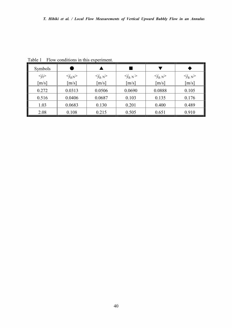
Table 1. Flow conditions in this experiment.
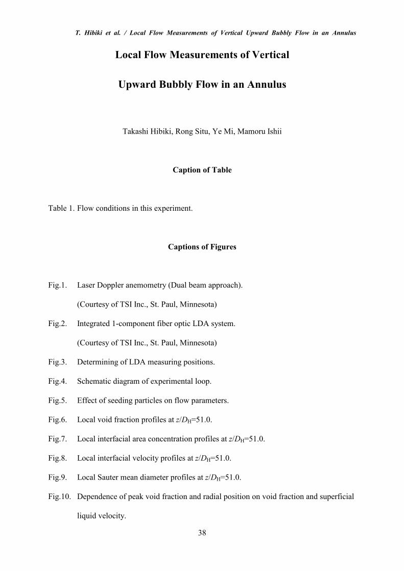
Captions of Figures
Fig.1. Laser Doppler anemometry (Dual beam approach).
(Courtesy of TSI Inc., St. Paul, Minnesota)
Fig.2. Integrated 1-component fiber optic LDA system.
(Courtesy of TSI Inc., St. Paul, Minnesota)
Fig.3. Determining of LDA measuring positions.
Fig.4. Schematic diagram of experimental loop.
Fig.5. Effect of seeding particles on flow parameters.
Fig.6. Local void fraction profiles at z/DH=51.0.
Fig.7. Local interfacial area concentration profiles at z/DH=51.0.
Fig.8. Local interfacial velocity profiles at z/DH=51.0.
Fig.9. Local Sauter mean diameter profiles at z/DH=51.0.
Fig.10. Dependence of peak void fraction and radial position on void fraction and superficial
liquid velocity.
T. Hibiki et al. / Local Flow Measurements of Vertical Upward Bubbly Flow in an Annulus
39
Fig.11. Maps of phase distribution patterns.
Fig.12. Dependence of interfacial velocity profile on void fraction and superficial liquid
velocity.
Fig.13. Local liquid velocity profiles at z/DH=51.0.
Fig.14. Local turbulence intensity profiles at z/DH=51.0.
Fig.15 Comparison of constitutive equation for distribution parameter in bubbly flow regime
with distribution parameters determined experimentally.
Fig.16 Comparison of semi-theoretical correlation for Sauter mean diameter with Sauter
mean diameters determined experimentally.
Fig.17 Comparison of constitutive equation for drift velocity in bubbly flow regime with
drift velocities determined experimentally.
T. Hibiki et al. / Local Flow Measurements of Vertical Upward Bubbly Flow in an Annulus
40
Table 1 Flow conditions in this experiment.
Symbols ● ▲ ■ ▼ ◆
<jf>
[m/s]
<jg,N>
[m/s]
<jg, N>
[m/s]
<jg, N >
[m/s]
<jg, N>
[m/s]
<jg, N>
[m/s]
0.272 0.0313 0.0506 0.0690 0.0888 0.105
0.516 0.0406 0.0687 0.103 0.135 0.176
1.03 0.0683 0.130 0.201 0.400 0.489
2.08 0.108 0.215 0.505 0.651 0.910
T. Hibiki et al. / Local Flow Measurements of Vertical Upward Bubbly Flow in an Annulus
41
Fig.1
T. Hibiki et al. / Local Flow Measurements of Vertical Upward Bubbly Flow in an Annulus
42
Fig.2
T. Hibiki et al. / Local Flow Measurements of Vertical Upward Bubbly Flow in an Annulus
43
Fig.3
Position A' Position C'
LDA Probe
Heater Rod Tube
Traversing Direction
A
B
C
D A' C'
E F x
y
(a) Top View of the Test Section
(b) Side View of the Test Section
T. Hibiki et al. / Local Flow Measurements of Vertical Upward Bubbly Flow in an Annulus
44
HeaterCooler
Flexible
Pipe
Separation
Tank
MainTank
Flowmeter PumpHeater
Rod
Height
Adjuster
Test
Section
Air Supply
T.C.
Filter
Drain
Degasing
Cooler
Drain
Drain
T.C.
T.C. T.C.
Condensation
TankD.P.
Air Flowmeters
P
P
Fig.4
T. Hibiki et al. / Local Flow Measurements of Vertical Upward Bubbly Flow in an Annulus
45
Fig.5
0.0 0.2 0.4 0.6 0.8 1.00.00
0.05
0.10
0.15
0.20
<jf>=0.50 m/s, <j
g>=0.0835 m/s
z/DH=40.3
No Seed
Seed
Void Fraction, α [-]
Radial Position, r/(R-R0)
0.0 0.2 0.4 0.6 0.8 1.00
100
200
300
400
<jf>=0.50 m/s, <j
g>=0.0835 m/s
z/DH=40.3
No Seed
Seed
Interfacial Area Conc., ai [m
-1]
Radial Position, r/(R-R0)
0.0 0.2 0.4 0.6 0.8 1.00.0
0.5
1.0
1.5
<jf>=0.50 m/s, <j
g>=0.0835 m/s
z/DH=40.3
No Seed
Seed
Gas Velocity, v g [m/s]
Radial Position, r/(R-R0)
0.0 0.2 0.4 0.6 0.8 1.00.0
0.5
1.0
1.5
2.0
2.5
3.0
3.5
4.0
4.5
5.0
<jf>=0.50 m/s, <j
g>=0.0835 m/s
z/DH=40.3
No Seed
Seed
Sauter Mean Dia., D
Sm [-]
Radial Position, r/(R-R0)
T. Hibiki et al. / Local Flow Measurements of Vertical Upward Bubbly Flow in an Annulus
46
Fig.6
0.0 0.2 0.4 0.6 0.8 1.00.0
0.1
0.2
0.3
0.4
0.5
0.6
<jf>=0.272 m/s
DH=19.1 mm
z/DH=51.0
Tim
e-Averaged Void Fraction, α [-]
0.0 0.2 0.4 0.6 0.8 1.00.0
0.1
0.2
0.3
0.4
0.5
0.6
<jf>=0.516 m/s
DH=19.1 mm
z/DH=51.0
0.0 0.2 0.4 0.6 0.8 1.00.0
0.1
0.2
0.3
0.4
0.5
0.6
<jf>=1.03 m/s
DH=19.1 mm
z/DH=51.0
Radial Position, r/(R-R0) [-]
0.0 0.2 0.4 0.6 0.8 1.00.0
0.1
0.2
0.3
0.4
0.5
0.6
<jf>=2.08 m/s
DH=19.1 mm
z/DH=51.0
T. Hibiki et al. / Local Flow Measurements of Vertical Upward Bubbly Flow in an Annulus
47
Fig.7
0.0 0.2 0.4 0.6 0.8 1.00
500
1000
1500
<jf>=0.272 m/s
DH=19.1 mm
z/DH=51.0
Tim
e-Averaged IAC, ai [m
-1]
0.0 0.2 0.4 0.6 0.8 1.00
500
1000
1500
<jf>=0.516 m/s
DH=19.1 mm
z/DH=51.0
0.0 0.2 0.4 0.6 0.8 1.00
500
1000
1500
<jf>=1.03 m/s
DH=19.1 mm
z/DH=51.0
Radial Position, r/(R-R0) [-]
0.0 0.2 0.4 0.6 0.8 1.00
500
1000
1500
<jf>=2.08 m/s
DH=19.1 mm
z/DH=51.0
T. Hibiki et al. / Local Flow Measurements of Vertical Upward Bubbly Flow in an Annulus
48
Fig.8
0.0 0.2 0.4 0.6 0.8 1.00.0
0.1
0.2
0.3
0.4
0.5
0.6
0.7
0.8
0.9
1.0
<jf>=0.272 m/s
DH=19.1 mm
z/DH=51.0
Tim
e-Averaged Interfacial Velocity, v g [m/s]
0.0 0.2 0.4 0.6 0.8 1.00.0
0.5
1.0
1.5
<jf>=0.516 m/s
DH=19.1 mm
z/DH=51.0
0.0 0.2 0.4 0.6 0.8 1.00.0
0.5
1.0
1.5
2.0
2.5
3.0
<jf>=1.03 m/s
DH=19.1 mm
z/DH=51.0
Radial Position, r/(R-R0) [-]
0.0 0.2 0.4 0.6 0.8 1.00
1
2
3
4
5
<jf>=2.08 m/s
DH=19.1 mm
z/DH=51.0
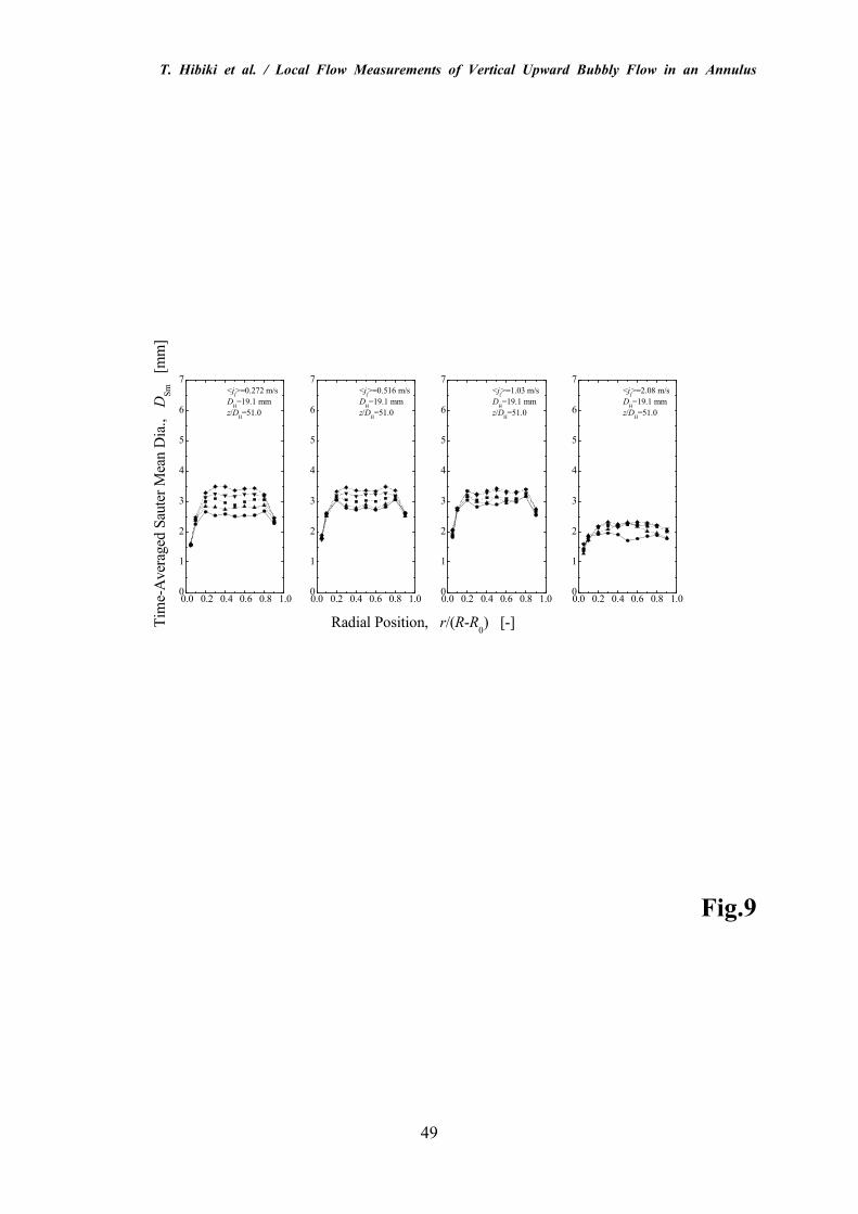
T. Hibiki et al. / Local Flow Measurements of Vertical Upward Bubbly Flow in an Annulus
49
Fig.9
0.0 0.2 0.4 0.6 0.8 1.00
1
2
3
4
5
6
7
<jf>=0.272 m/s
DH=19.1 mm
z/DH=51.0
Tim
e-Averaged Sauter Mean Dia., D
Sm [mm]
0.0 0.2 0.4 0.6 0.8 1.00
1
2
3
4
5
6
7
<jf>=0.516 m/s
DH=19.1 mm
z/DH=51.0
0.0 0.2 0.4 0.6 0.8 1.00
1
2
3
4
5
6
7
<jf>=1.03 m/s
DH=19.1 mm
z/DH=51.0
Radial Position, r/(R-R0) [-]
0.0 0.2 0.4 0.6 0.8 1.00
1
2
3
4
5
6
7
<jf>=2.08 m/s
DH=19.1 mm
z/DH=51.0
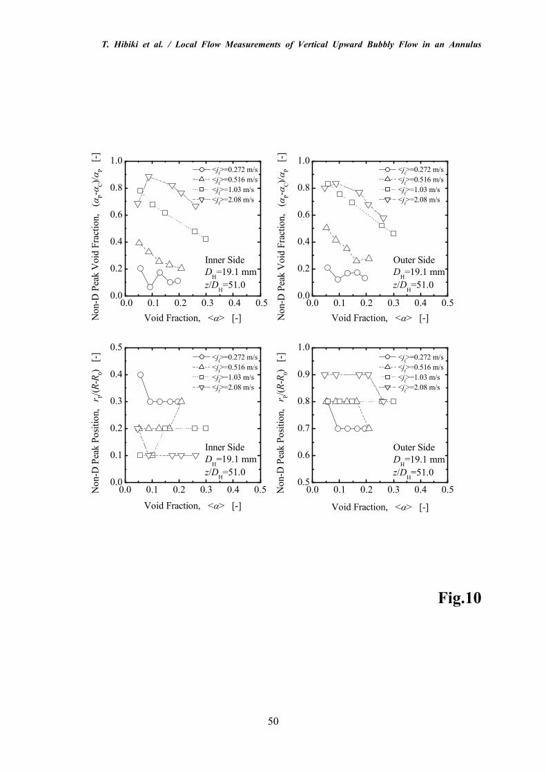
T. Hibiki et al. / Local Flow Measurements of Vertical Upward Bubbly Flow in an Annulus
50
Fig.10
0.0 0.1 0.2 0.3 0.4 0.50.0
0.2
0.4
0.6
0.8
1.0
Inner Side
DH=19.1 mm
z/DH=51.0
<jf>=0.272 m/s
<jf>=0.516 m/s
<jf>=1.03 m/s
<jf>=2.08 m/s
Non-D
Peak Void Fraction, (α
P-α
C)/αP [-]
Void Fraction, <α> [-]
0.0 0.1 0.2 0.3 0.4 0.50.0
0.2
0.4
0.6
0.8
1.0
Outer Side
DH=19.1 mm
z/DH=51.0
Outer Side
DH=19.1 mm
z/DH=51.0
<jf>=0.272 m/s
<jf>=0.516 m/s
<jf>=1.03 m/s
<jf>=2.08 m/s
Non-D
Peak Void Fraction, (α
P-α
C)/αP [-]
Void Fraction, <α> [-]
0.0 0.1 0.2 0.3 0.4 0.50.0
0.1
0.2
0.3
0.4
0.5
Inner Side
DH=19.1 mm
z/DH=51.0
<jf>=0.272 m/s
<jf>=0.516 m/s
<jf>=1.03 m/s
<jf>=2.08 m/s
Non-D
Peak Position, r P/(
R-R
0) [-]
Void Fraction, <α> [-]
0.0 0.1 0.2 0.3 0.4 0.50.5
0.6
0.7
0.8
0.9
1.0 <j
f>=0.272 m/s
<jf>=0.516 m/s
<jf>=1.03 m/s
<jf>=2.08 m/s
Non-D
Peak Position, r P/(
R-R
0) [-]
Void Fraction, <α> [-]
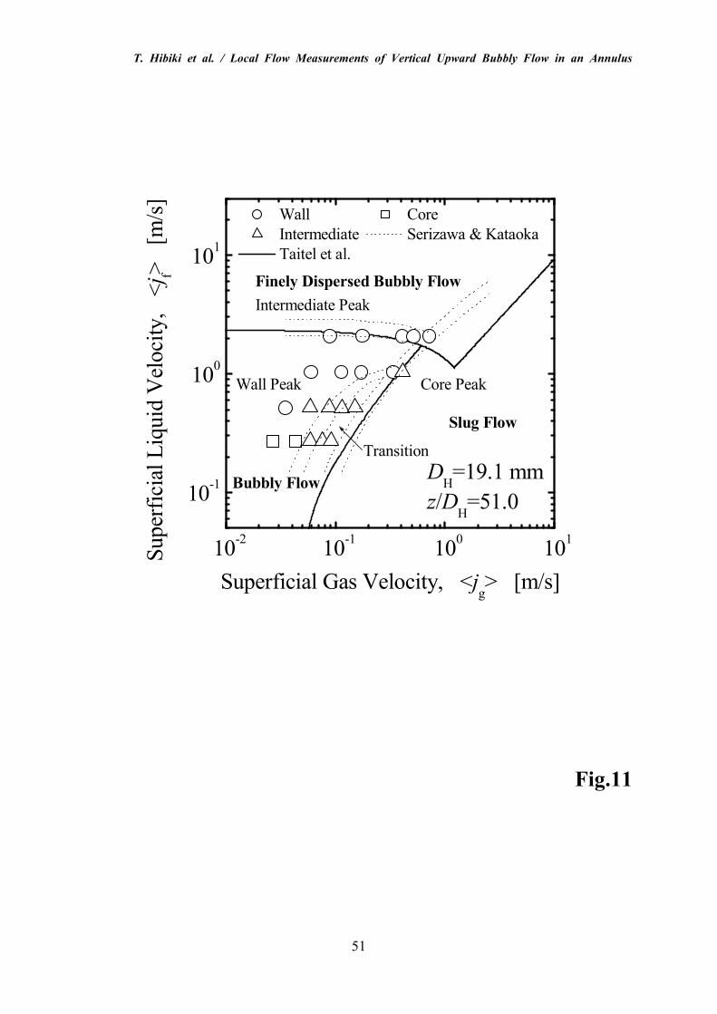
T. Hibiki et al. / Local Flow Measurements of Vertical Upward Bubbly Flow in an Annulus
51
Fig.11
10-2
10-1
100
101
10-1
100
101
Core Peak
Intermediate Peak
Wall Peak
Transition
Slug Flow
Bubbly Flow
Finely Dispersed Bubbly Flow
DH=19.1 mm
z/DH=51.0
Core
Serizawa & Kataoka
Wall
Intermediate
Taitel et al.
Superficial Liquid Velocity, <j f> [m/s]
Superficial Gas Velocity, <jg> [m/s]

T. Hibiki et al. / Local Flow Measurements of Vertical Upward Bubbly Flow in an Annulus
52
Fig.12
0.0 0.1 0.2 0.3 0.40
5
10
15
z/DH=51.0
DH=19.1 mm
<jf>=0.272 m/s
<jf>=0.516 m/s
<jf>=1.03 m/s
<jf>=2.08 m/s
Exponent, n [-]
Void Fraction, <α> [-]
0.0 0.5 1.0 1.5 2.0 2.50
5
10
15
z/DH=51.0
DH=19.1 mm
<α>=0.050 <α>=0.10 <α>=0.15
Exponent, n [-]
Superficial Liquid Velocity, <jf> [m/s]
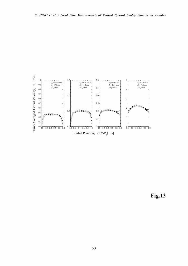
T. Hibiki et al. / Local Flow Measurements of Vertical Upward Bubbly Flow in an Annulus
53
Fig.13
0.0 0.2 0.4 0.6 0.8 1.00.0
0.1
0.2
0.3
0.4
0.5
0.6
0.7
0.8
0.9
1.0
<jf>=0.272 m/s
DH=19.1 mm
z/DH=49.8
Tim
e-Averaged Liquid Velocity, v f [m/s]
0.0 0.2 0.4 0.6 0.8 1.00.0
0.5
1.0
1.5
<jf>=0.516 m/s
DH=19.1 mm
z/DH=49.8
0.0 0.2 0.4 0.6 0.8 1.00.0
0.5
1.0
1.5
2.0
2.5
3.0
<jf>=1.03 m/s
DH=19.1 mm
z/DH=49.8
Radial Position, r/(R-R0) [-]
0.0 0.2 0.4 0.6 0.8 1.00
1
2
3
4
5
<jf>=2.08 m/s
DH=19.1 mm
z/DH=49.8
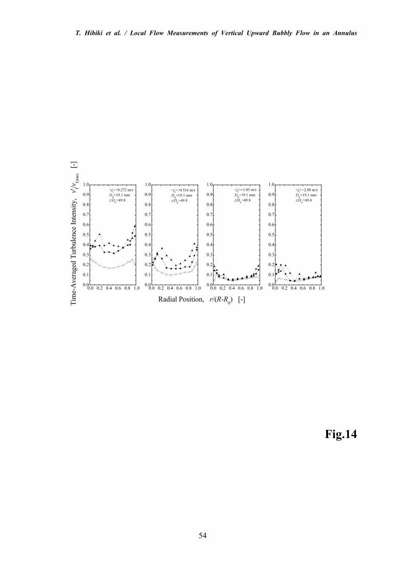
T. Hibiki et al. / Local Flow Measurements of Vertical Upward Bubbly Flow in an Annulus
54
Fig.14
0.0 0.2 0.4 0.6 0.8 1.00.0
0.1
0.2
0.3
0.4
0.5
0.6
0.7
0.8
0.9
1.0
<jf>=0.272 m/s
DH=19.1 mm
z/DH=49.8
Tim
e-Averaged Turbulence Intensity, v'f/v
f,max [-]
0.0 0.2 0.4 0.6 0.8 1.00.0
0.1
0.2
0.3
0.4
0.5
0.6
0.7
0.8
0.9
1.0
<jf>=0.516 m/s
DH=19.1 mm
z/DH=49.8
0.0 0.2 0.4 0.6 0.8 1.00.0
0.1
0.2
0.3
0.4
0.5
0.6
0.7
0.8
0.9
1.0
<jf>=1.03 m/s
DH=19.1 mm
z/DH=49.8
Radial Position, r/(R-R0) [-]
0.0 0.2 0.4 0.6 0.8 1.00.0
0.1
0.2
0.3
0.4
0.5
0.6
0.7
0.8
0.9
1.0
<jf>=2.08 m/s
DH=19.1 mm
z/DH=49.8
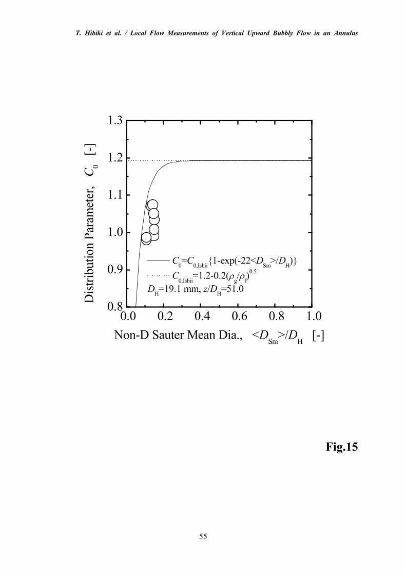
T. Hibiki et al. / Local Flow Measurements of Vertical Upward Bubbly Flow in an Annulus
55
Fig.15
0.0 0.2 0.4 0.6 0.8 1.00.8
0.9
1.0
1.1
1.2
1.3
C0=C
0,Ishii{1-exp(-22<D
Sm>/D
H)}
C0,Ishii
=1.2-0.2(ρg/ρ
f)0.5
DH=19.1 mm, z/D
H=51.0
Distribution Param
eter, C
0 [-]
Non-D Sauter Mean Dia., <DSm>/D
H [-]
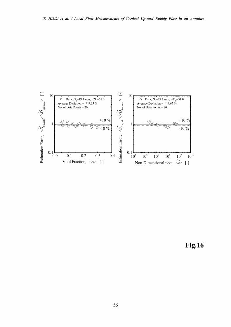
T. Hibiki et al. / Local Flow Measurements of Vertical Upward Bubbly Flow in an Annulus
56
Fig.16
0.0 0.1 0.2 0.3 0.40.1
1
10
~~~
~
Data, DH=19.1 mm, z/D
H=51.0
Average Deviation = ±9.65 %
No. of Data Points = 20
-10 %
+10 %
Estim
ation Error, <
DSm,calc.>/<
DSm,meas.> [-]
Void Fraction, <α> [-]10
510
610
710
810
910
100.1
1
10
~
Data, DH=19.1 mm, z/D
H=51.0
Average Deviation = ±9.65 %
No. of Data Points = 20
-10 %
+10 %Estim
ation Error, <
DSm,calc.>/<
DSm,meas.> [-]
Non-Dimensional <ε>, <ε> [-]
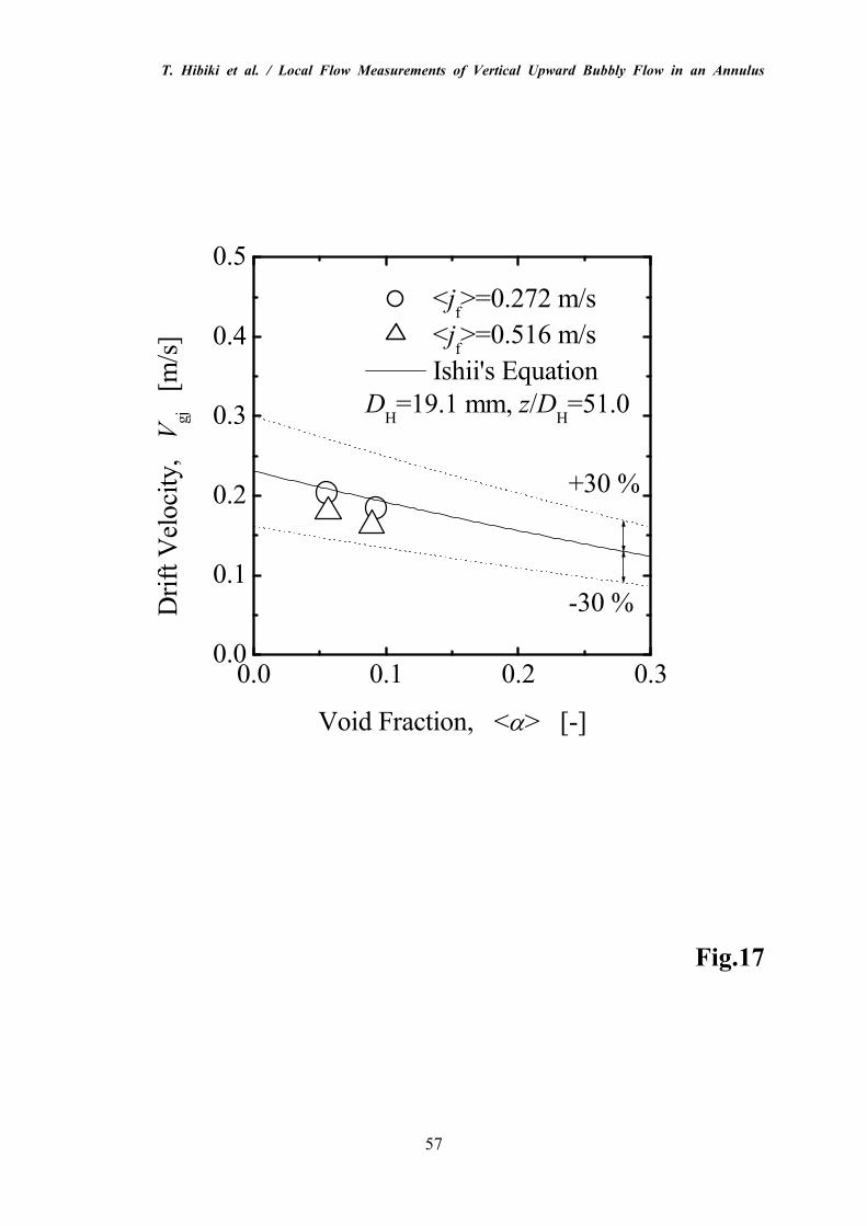
T. Hibiki et al. / Local Flow Measurements of Vertical Upward Bubbly Flow in an Annulus
57
Fig.17
0.0 0.1 0.2 0.30.0
0.1
0.2
0.3
0.4
0.5
<jf>=0.272 m/s
<jf>=0.516 m/s
Ishii's Equation
DH=19.1 mm, z/D
H=51.0
-30 %
+30 %
Drift Velocity, Vgj [m/s]
Void Fraction, <α> [-]