1

Three-dimensional numerical model of heat losses from district heating network pre-insulated pipes

buried in the ground

J. Danielewicz1, B. Śniechowska

1, M.A. Sayegh

1, N. Fidorów

1, H. Jouhara

2*

1Institute of Air Conditioning and District Heating, Faculty of Environmental Engineering, Wrocław University of Technology, C. K. Norwida St. 4/6, 50-

373 Wrocław, Poland

2Institute of Energy Futures, RCUK Centre for Sustainable Energy Use in Food Chains (CSEF), Brunel University, Uxbridge, Middlesex UB8 3PH, UK,

E-mail: hussam.jouhara@brunel.ac.uk , Tel: +44 (0) 1895267805; Fax: +44 (0) 1895 269777.

*Corresponding Author

ABSTRACT

The purpose of the paper is to investigate the challenges in modeling the energy losses of heating networks and to

analyse the factors that influence them. The verification of the simulation was conducted on a test stand in-situ and based

on the measurements of the testing station, a database for the final version of the numerical model was developed and a

series of simulations were performed. Examples of the calculated results are shown in the graphs. The paper presents an

innovative method of identify the energy losses of underground heating network pipelines and quantify the temperature

distribution around them, in transient working conditions. The presented method makes use of numerical models and

measured data of actual objects.

The dimensions of the pipelines used were six meters wide, eight meters high and one meter in depth, while they were

simulated under conditions of zero heat flow in the ground, in the perpendicular to the sides direction of the calculated

area and considering the effects of ground’s thermal conductivity. The mesh was developed using advanced functions,

which resulted its high quality with the average orthogonal quality of 0.99 (close to 1.00) and Skewness of 0.05 (between

0.00 and 0.25). To achieve better accuracy of the simulation model, the initial conditions were determined based on the

numerical results of a three-dimensional analysis of heat losses, in steady state conditions in a single moment. The

validation process confirmed the high quality of the model, as the differences between the ground temperatures were

approximately 0.1 °C.

Nomenclature

c specific heat kJ/(kg·K)

dwt pipe wall thickness m

DN nominal diameter m

Di outer diameter of insulation m

Do outer diameter of pipe casing m

Dinn inner diameter of the pipe m

Dout outer diameter of the pipe m

S distance m

T, t Temperature °C

Ts network supply water temperature °C

Tr network return water temperature °C

to outside air temperature °C

ta ambient pipeline temperature °C

Tgs ground surface temperature °C

tgr ground temperature °C

w soil moisture %

wv volumetric soil moisture kg/m3

nV network water volume flow m3/s

vw wind velocity at the ground surface m/s

*

2

ΔX length of the pitch element m

Greek symbols

ρ Density kg/m3

α convective heat transfer coefficient W/(m2·K)

λ thermal conductivity coefficient W/(m·K)

1 INTRODUCTION

1.1 District heating and district heating networks characteristics

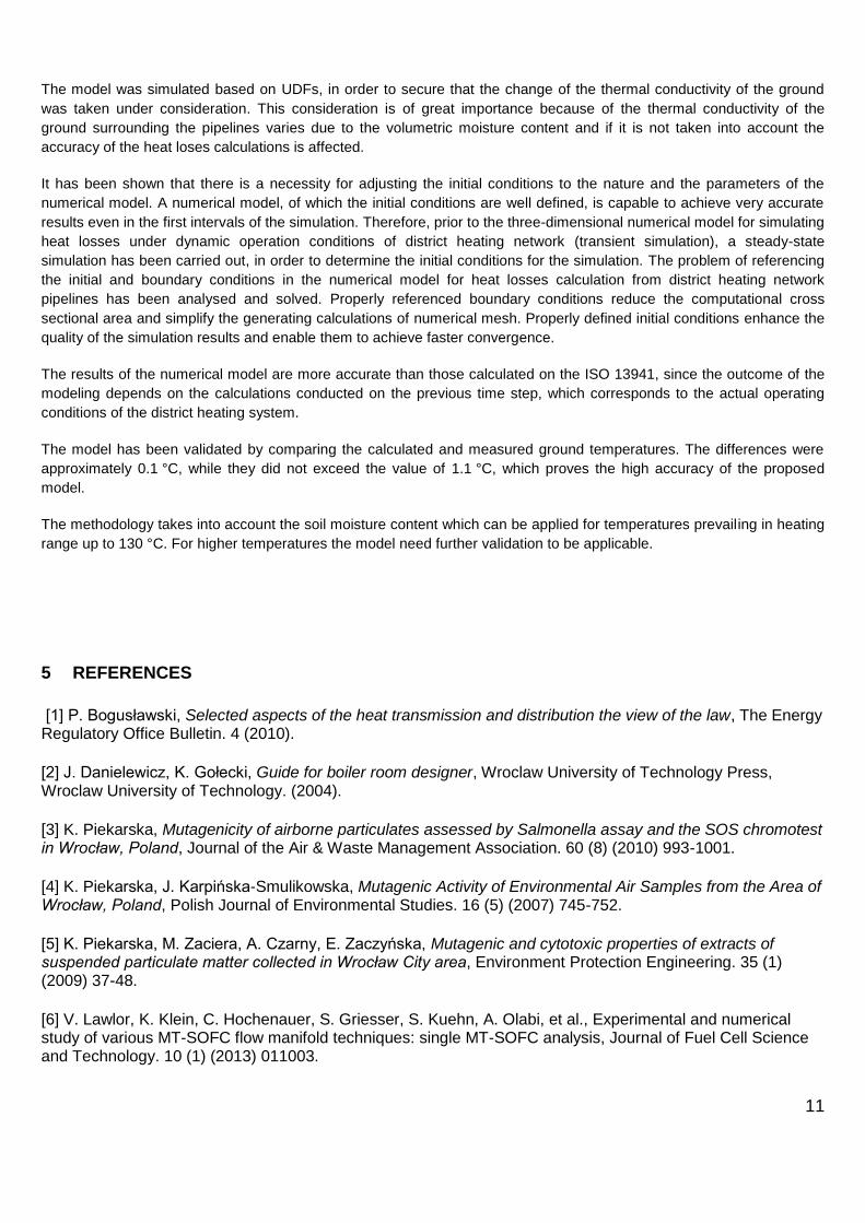
The heating network of Poland provides centralised district heating to more than 300 cities and 15 million residents [1,2].

Figure 1 shows the percentage use of district heating systems for the heating needs supplement in selected countries.

According to the figure, the production and distribution of heat in centralised heating systems cover 95%, 60% and 52%

of the needs in Iceland, Denmark and Poland, respectively [1].

In Poland, the vast majority of district heating systems use coal as an energy source, despite the fact that the process of

its combustion generates air pollution; however, it should be mentioned that such systems confer the possibility of

exhaust gases purification. In addition, gases and dusts emitted to the atmosphere have adverse effects on living

organisms. Furthermore, the surface of the suspended particulates can adsorb organic compounds of different chemical

classes forming a complex mixture of unknown biological properties [3-9]. Even so, for many years to come coal will be

one of the basic energy sources for the production of electricity and heat.

The network transmission and distribution of heat loss is one of the key factors in the optimal design of district heating

systems, which includes various pipe configurations, like flexible pre-insulated twin pipes with symmetrical or

asymmetrical insulation, double pipes, triple pipes and a 2D-modeling analysis of pipes in computer software with the use

of the finite element method (FEM) [10-12].

One of the means to improve the energy efficiency of district heating is to reduce the heat losses at the transmission

(distribution), which will lead to a more sustainable and efficient designs of district heating networks [13-17]. For district

heating application the following types of construction may be distinguished [18,19]:

overhead – located above the ground on poles or any other supporting structures,

aboveground – arranged on the foundations, directly on the ground surface,

underground – located in the ground and arranged in the tunnels or district heating channels, and placed directly

in the ground (such as pre-insulated pipe technologies).

Currently, the most common configuration of placing pipelines is their direct placement in the ground. In contrast, above-

ground systems are implemented only in exceptional cases, when underground systems show lack of technical feasibility

or their operating cost is considered to be unaffordable.

1.2 Heat losses in district heating networks

The main factor influencing the energy losses of heating networks is network leakages, which cause the water to diverge

from its channel and to transfer the heat from the interior of pipelines to the environment.

Heat losses occurring as a result of network water losses refer to both network and heat distribution units, as well as

internal central heating systems supplied directly from the network. The main cause of network water loss can be "micro-

damages" in the pipelines; leakages of the heat sources, the heat distribution units or the main pipelines, as well as

leakages of working fluid caused by a breakdown removal or planned repairs [20].

3

Based on the presented data of figure 3, the average rate of heat losses lies within the range of 7.6% to 27.8%. On the

basis of references and conducted analysis, it was found that [21]:

Due to simplified assumptions concerning the input data, the theoretical calculations may not reflect the real heat

losses occurring in the operated district heating systems.

Due to the lack of clear opinion concerning the temperature of the piping surrounding used in the calculations of

the heat loss, the problem of reference temperature of the ground should be solved.

The thermal conductivity of the soil, surrounding the pre-insulated piping, may have a significant impact on the

results of the heat loss calculation; for this reason, the calculations should take into account the correct thermal

conductivity around the pipe buried in the ground. This is particularly important in the case of modeling the

dynamic working conditions of the district heating network.

The steady state analysis does not reflect the actual working conditions of district heating network; it represents

only the state, which occurs under certain conditions.

The described analytical methods determine the heat losses, do not provide accurate results in the case of the

transient heat transfer [21]; to compensate any discrepancies between the theoretical and the actual heat losses,

the application of numerical computational methods and the use of actual data should be examined.

The accuracy of numerical methods varies and depends on the method of calculations and the boundary and

initial conditions of the model.

Based on previous studies, it was found that the fulfillment of the main objective of the work described in the paper

requires the implementation of the following tasks:

Design, construction and commission of the research measuring stand in the real district heating system.

Development of a numerical model, taking into account the measurement data, for analysing the heat transfer in

pre-insulated district heating pipelines buried in the ground.

Identification and justification of the proposed boundary and initial conditions for the numerical model.

Verification of the numerical model based on experimental studies.

2 MATERIALS AND METHODS

2.1 Test facility design

Figure 4 shows the schematic diagram of the measuring station, located in the lecture building of Wroclaw University of

Technology, which consists of the following elements:

The measuring and collection system for the ground temperature,

The measuring and collection system for the outdoor air temperature,

The measuring and collection system for the volumetric humidity of the soil around the pipeline,

The measuring system in the heat transfer station (for the district heating water temperature and flow).

The district heating of the building includes two pre-insulated pipes with nominal diameter of DN 40, which consists of a

steel carrier pipe, thermal insulated with rigid polyurethane foam (PUR) and an outer pipe jacket of high density

polyethylene (PE-HD). The dimensions of each component of the pipes are given in Table 1. The distance between the

pipes’ outer coats equals to 19 cm.

The temperature measurement in the ground takes into account only the ground area that surrounds the pipelines. The

sensors have been installed in the soil, which can be characterized as a uniform environment along the whole district

heating network. The temperature measurement around the pipes was carried out by the temperature sensors IT-CF1

with the transduction element (thermo resistor) Pt100, connected to four channels of the Smart Reader Plus 10 recorder.

Three Pt100 sensors were used for measuring the temperature in the ground, while the fourth sensor was used to

4

measure the outdoor air temperature. The outside air temperature sensor was located approximately 15 cm above the

ground surface in the same vertical plane, where in the ground temperature sensors were located. Measurements were

taken every 10 minutes, saved in the internal Smart Reader Plus 10 memory logger and later on they were imported to

the computer.

For the recording of the volumetric soil moisture around the pre-insulated district heating pipelines, six ECHO 5-TM

probes, and two EM-50 data recorders were used, along with the Echo2 Utility PC software of Decagon Devices Inc. for

configuring the data. The measurements of the volumetric soil moisture were programmed with an interval of 10 minutes.

After reaching the measurement time, the registration system calculated the average of the readings performed every 60

seconds.

The heat transfer station, located in the Kamstrup Multical Building, was implemented with a 601- type heat meter,

equipped with a pair of Pt 500 temperature sensors and an Ultra flow 65-S/R flow sensor. The registration system used

for the data recording had two carriers, one on the hard disk of the microcomputer and one on the SD memory card. For

reading and recording the data, the software "Rejestrator LC" was used.

The heating operation monitoring system has been used for recording and archiving the following data:

The district heating network supply water temperature (Ts)

The district heating network return water temperature (Tr)

Network water volume flow ( )

Data were collected and recorded continuously with a time step of 10 minutes.

2.2 The three-dimensional numerical model

CFD modelling of pre-insulated pipes in the ground is a multistage process requiring a number of operations. Numerical

modeling was performed using ANSYS 14.5 [22,23] package, with the FLUENT computational software (solver).

Elaboration of the numerical model in ANSYS/Fluent environment required to complete the following steps [21]:

Elaboration of computational geometry, including the definition of proper dimensions and boundary conditions.

Constructing a numerical mesh (discretization of the geometric area) using advanced options (Fixed, Mapped,

Sizing) for the mesh construction. The mesh quality has been checked using two parameters Orthogonal Quality

and Skewness.

Preparation and characterisation of all calculation domains by defining the thermal and physical properties of all

materials used in the model.

Introduction of additional user defined algorithms in ANSYS/ developed in C++ programing environment and

afterwards connected to the FLUENT solver.

Elaboration of input database using some of the data obtained from the test stand.

Selection of boundary and initial conditions: the ground temperature or thermodynamic behavior on the edges

and fluid temperature and velocity in the pipelines.

Implementation of numerical calculations with an appropriate time step and correct number of iterations.

Elaboration of computational simulation results.

Verification of the results obtained from the numerical model.

5

3 RESULTS AND DISCUSSION

Network transmission and distribution heat loss estimation is a key factor in the design optemisation process of district

heating systems. The reported work addresses this by the development of a 3D computer model that will precisely predict

such losses from the district heating network’s pre-insulated pipes. The developed methodology enables the selection of

the impact area’s temperature of pipelines and takes into account the temperature field variations of the ground that

surrounds the pipelines.

The main purpose of this paper is to show the process and the results of developing a three-dimentional model, which

simulates the heat losses of a district heating network with pre-insulated pipes burried in the ground. Therefore, the

results section is divided into three parts concerning the development of the model, the simulation results and the model

validation.

3.1 Model development

3.1.1 Geometry area sizing analysis

The selection of the appropriate pipes’ cross sectional area is one of the main factors that influence the profile of

temperature distribution of the ground around the district heating network. The difficulty related to the geometrical

dimensions of the pipes’ area, is also related to the choice of the proper boundary conditions on the lateral surfaces

(edges) of their area. Two stages analysis facilitates procedure of geometry size selection.

The first stage of the analysis refers to the selection of appropriate boundary conditions and matching geometrical

dimensions; areas of different widths are analysed assuming boundary condition of first kind. The rate of network supply

and return water temperatures was set as follow: Ts/Tr = 130/70°C. The temperature distribution around the pre-insulated

district heating pipes have been calculated for an exemplary diameter of DN 40 and constant values of soil temperature at

the lateral edges (tgr = 10°C).

Figure 5 presents the graphical results of numerical calculations for exemplary geometric area of four meters high and

two meters wide. Based on the results, it can be concluded that the fixed temperature at the side edges of the area

interferes with the temperature distribution in the ground. However, these surfaces do not show such temperature

distribution in real conditions, due to the fact that the ground temperature changes with the increase of depth, and

stabilises after a certain point [24,25]. Moreover, constant temperature at the side edges of the area with too narrow

geometrical area contributes to fluctuations of the temperature distribution in the soil.

With the proposed approach, proper temperature distribution profiles are obtained as long as one of the initial boundary

conditions of the numerical model considers the temperature distribution of the ground and the width of the pipes is big

enough. However, the implementation of large geometry dimensions (100 or 200 m) may cause difficulties in the

discretization stage of the geometrical area and in the generation of high quality mesh, resulting increase of the

simulation time. This problem can be solved by changing the boundary condition from first to second kind. One of the

assumptions of the new approach is zero heat flow in the ground in the direction perpendicular to the sides of the

calculation area. Thus, the significant reduction of the distance of lateral surfaces of the geometrical area from the

pipelines is possible.

Based on the simulations, the geometry dimensions of the computational model have been estimated using the second

approach to the boundary conditions. Initially, three different values were adopted for the geometrical width (2, 5 and

10 m) for the given boundary condition of the second kind on the lateral edges of the geometrical area. Depth of eight

meters of the ground has been assumed in all cases. This approach allowed the assumption of constant temperature for

the bottom edge of computing area (tgr = 8 °C) [19,26,27]. The input data was assumed as exemplary values of the

external temperature (to = -15.7 °C) and network temperatures (Ts/Tr = 125.2/66.4 °C), which have been registered on the

test stand during heating season. Figure 6 presents the results of the temperature distribution analysis of the ground

around the district heating networks.

6

On figures 8, 9 and 10, it can be seen that in the models of 5 and 10 meters the isothermal lines have similar distribution.

Models with two meters width may be too narrow. The calculation results presented in Figure 6 are only the graphical

representation of the performed simulations. For this reason, the charts are additionally supplemented with vertical

temperature profiles situated in different distances in relation to the district heating network (the distribution of profiles is

presented on the diagram in Figure 7).

The discrepancies in the results of the temperature distribution are particularly evident in the geometric model with the

two meters width rather than the models of five and ten meters wide. Between the models of five and ten meters wide, the

differences are considerably small. The mean percentage error for models of five and ten meters wide is approximately

1.5%, while for models of two and ten meters wide is about 21%. In order to reduce the impact of errors on the results,

and maintain small geometric dimensions, the specifications of the five meters model have been increased by 1 meter.

The obtained temperature profiles were compared and the results of this comparison are shown in Figures 8 and 10. The

temperature distribution of the six meters wide model perfectly coincides with the distribution of the ten meters model. On

this basis, ultimately it has been assumed that the width of the area will be equal to 6 meters.

Based on the previous analysis, the numerical calculations will be carried out in the model of six meters width, eight

meters high and one meter depth.

3.1.2 Discretization

The development of computational mesh is a crucial task before define the boundary conditions and start the calculation

process. The stage of discretization is of great importance and the success of the whole computational procedure

depends on it. In ANSYS 14.5 PC application, it is possible to generate the mesh automatically or developing it

independently based on available advanced auxiliary options offered by the program.

Due to the low quality of the mesh generated by the program, it has been decided to use the advanced options for the

mesh construction.

Numerical mesh can be created from various kinds of computational cells. Most frequently used are the following types

[28,29]:

"Tetra" – tetrahedral, in the form of pyramid with a triangle base.

"Hexa" - hexahedral, in the form of a prism with quadrilateral base.

"Pyramid"/"Penta" – in the form of pyramid with quadrilateral base.

"Prism"/"Wedge" – in the form of a prism with triangle base (so called Prism).

In discretization the most often chosen element is the simplest one with four nodes (“Tetra”), however it is not

recommended [29]. "Tetra" elements are not adaptable, and using them for discrete models can increase the level of

errors [29]. The best results can be obtained by subdividing the space into six-sided blocks, with hexahedral cells

("Hexa"). Each mesh needs a quality check, because it can affect the accuracy and stability of the subsequent numerical

calculations. The mesh can be considered as correct when the calculated results do not depend on it. The calculation

mesh has been selected based on performed convergence test. Six different numerical meshes with various size and

number of computational cells were analysed. Finally, the mesh with the minimum effect on the calculated results was

selected, which consists of 2,847,777 nodes and 2,770,800 computational "Hexa" type cells, as shown in Figure 11.

Fixed option, allows the user to define his own values of the mesh parameters and this method was firstly used.

Therefore, the following parameters of the mesh have been assumed:

Max face sizing (the preferred size of a single computational cell in the mesh) is equal to 0.05 m.

Max size (the maximum size of a single computational cell in the mesh) is equal to 0.1 m.

7

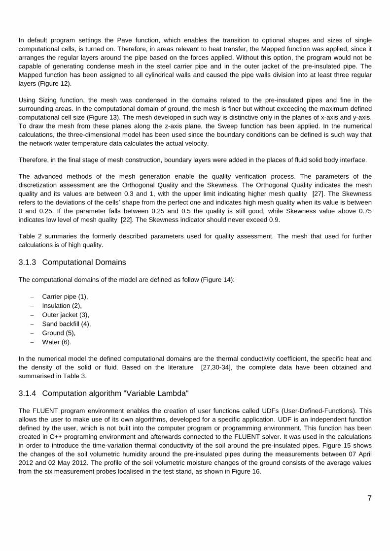
In default program settings the Pave function, which enables the transition to optional shapes and sizes of single

computational cells, is turned on. Therefore, in areas relevant to heat transfer, the Mapped function was applied, since it

arranges the regular layers around the pipe based on the forces applied. Without this option, the program would not be

capable of generating condense mesh in the steel carrier pipe and in the outer jacket of the pre-insulated pipe. The

Mapped function has been assigned to all cylindrical walls and caused the pipe walls division into at least three regular

layers (Figure 12).

Using Sizing function, the mesh was condensed in the domains related to the pre-insulated pipes and fine in the

surrounding areas. In the computational domain of ground, the mesh is finer but without exceeding the maximum defined

computational cell size (Figure 13). The mesh developed in such way is distinctive only in the planes of x-axis and y-axis.

To draw the mesh from these planes along the z-axis plane, the Sweep function has been applied. In the numerical

calculations, the three-dimensional model has been used since the boundary conditions can be defined is such way that

the network water temperature data calculates the actual velocity.

Therefore, in the final stage of mesh construction, boundary layers were added in the places of fluid solid body interface.

The advanced methods of the mesh generation enable the quality verification process. The parameters of the

discretization assessment are the Orthogonal Quality and the Skewness. The Orthogonal Quality indicates the mesh

quality and its values are between 0.3 and 1, with the upper limit indicating higher mesh quality [27]. The Skewness

refers to the deviations of the cells’ shape from the perfect one and indicates high mesh quality when its value is between

0 and 0.25. If the parameter falls between 0.25 and 0.5 the quality is still good, while Skewness value above 0.75

indicates low level of mesh quality [22]. The Skewness indicator should never exceed 0.9.

Table 2 summaries the formerly described parameters used for quality assessment. The mesh that used for further

calculations is of high quality.

3.1.3 Computational Domains

The computational domains of the model are defined as follow (Figure 14):

Carrier pipe (1),

Insulation (2),

Outer jacket (3),

Sand backfill (4),

Ground (5),

Water (6).

In the numerical model the defined computational domains are the thermal conductivity coefficient, the specific heat and

the density of the solid or fluid. Based on the literature [27,30-34], the complete data have been obtained and

summarised in Table 3.

3.1.4 Computation algorithm "Variable Lambda"

The FLUENT program environment enables the creation of user functions called UDFs (User-Defined-Functions). This

allows the user to make use of its own algorithms, developed for a specific application. UDF is an independent function

defined by the user, which is not built into the computer program or programming environment. This function has been

created in C++ programing environment and afterwards connected to the FLUENT solver. It was used in the calculations

in order to introduce the time-variation thermal conductivity of the soil around the pre-insulated pipes. Figure 15 shows

the changes of the soil volumetric humidity around the pre-insulated pipes during the measurements between 07 April

2012 and 02 May 2012. The profile of the soil volumetric moisture changes of the ground consists of the average values

from the six measurement probes localised in the test stand, as shown in Figure 16.

8

The average values of the ground volumetric moisture around the pre-insulated pipes were in the range of 14.9 - 17.8%.

Based on measurements, the approximation function describing the dependence of the ground thermal conductivity and

ground volumetric moisture was in the range of 10 % to 20 % (Figure 17).

Based on the measurements of ground volumetric moisture and the approximation function, the average values of ground

thermal conductivity around the pipes were calculated (Figure 18). These values were introduced using the “Variable

Lambda” software, written in C++ programing language, and assigned to the “sand backfill” computational domain.

3.1.5 Development of input database

The heat losses in district heating network connections were determined based on the assumptions made, regarding the

boundary conditions of the model (Section 3.1.6) and the parameters measured in the test stand, based on which the

input database was built. The database contains the following parameters:

Time.

Outside air temperature.

Supply water temperature.

Return water temperature.

Circulating water velocity calculated on the basis of the measured volumetric flow of network water.

Volumetric moisture of the soil around the pipeline.

The calculations were performed for the selected time period (19/04/2012 - 02/05/2012) with a single time step of Δt =

3600 second. On this basis, 1480 time steps were obtained and 20 iterations were carried out for each one of them.

Figuer 19 represents the measured network water temperature and the outside air temperature on the test stand within

the time period assumed for the analysis. Figure 20 shows the circulating water velocity in district heating network

connection, which has been calculated based on measurements registered by measuring system.

3.1.6 Boundary and initial conditions in the numerical model

Proper development of boundary and initial conditions is essential for the proper operation of the numerical model. Figure

21 represents the scheme, based on which the various types of boundary conditions of the computational model were

characterised.

According to the literature research [27,28], and on the outcomes of the simulation calculations at eight meters depth, the

ground temperature is constant during the whole year in Poland and is equal to 8 °C. Therefore, the first boundary

condition refers to the bottom plane of the model (4 - 3 - 7 - 8) and indicates that the temperature is constant on this

surface (t4-3-7-8 = 8°C). There is no reason for substantial incensement of the depth of ground in the model, because below

20 meters the ground temperature increases with the depth due to the thermal impact of earth’s core [35].

Another boundary condition is set on the sides, front and rear planes of the calculation area (1 - 2 - 3 - 4), (5 - 6 - 7 - 8), (1

- 3 - 7 - 5), (2 - 4 - 8 - 6), respectively. In CFD models based on numerical fluid mechanics, this type of condition is called

symmetry surfaces. These surfaces are characterised by zero momentum, mass and energy transfer towards orthogonal

direction.

On the upper surface of the ground (1 - 2 - 5 - 6), a heat transfer between the outdoor air and the ground occurs.

Because of that, a third boundary condition is implemented, which cause the dependency of the provision of the heat

transfer coefficient on the type of heat transfer which is occurring on the surface of the given body, the type of fluid, the

velocity and direction of fluid flow in relation to the surface of the body. Literature describes various approaches of the

heat transfer coefficient adoption in this case. Convection heat transfer coefficient can be calculated using so-called

Jürgers calculation formulas, depending on the wind velocity at the surface of the ground vw [34].

9

for

vw > 5 m/s (1)

for vw < 5 m/s (2)

According to the literature research, the values of heat transfer coefficient may be assumed depending on the wind

velocity. For a range of wind velocity values vw= 3.6 – 4.6 m/s, the heat transfer coefficient can be equal to αe = 13 – 14

W/(m2.K). Kvisgaard and Bøhm in their works assumed constant value of the heat transfer coefficient equal to αe = 14.6

W/(m2·K) [25,30,34,36]. In the calculation model, a constant value of heat transfer coefficient αe = 14.6 W/(m

2·K) has

been assumed [30,34,37,38].

The computational model requires also the introduction of boundary conditions on the inlets (9) and outlets (10) of two

carrier pipes. The "inlet" boundary condition requires defining the values of velocity and temperature. The temperature

profiles for inlets of network water were introduced based on the constructed input database. A developed velocity profile

of installation water on the supply and return pipeline has been assumed.

For the "outlet" boundary condition, constant static pressure and zero gradients of all dependent variables for

perpendicular direction to this border has been assumed in accordance to the guidelines for the adaptation of the

boundary conditions for CFD codes users [28].

Initial conditions are substantial in time transient analysis and refer to the distribution parameters at the beginning of the

process. The initial conditions for three-dimensional numerical model, which are used for heat loss calculations under

dynamic operation conditions of district heating network, has been determined based on the results obtained from three-

dimensional simulation model of the heat loss for steady state conditions in a single moment (time step 1). The results

obtained from the calculations of the model represent the steady-state conditions based on which the initial conditions of

three-dimensional model were defined. Based on the analysis performed below, it was found that the developed

initialization procedure of the numerical model calculations beneficially affect the time needed to achieve the convergence

of the model. In order to illustrate the consequences of the adoption of the default initial conditions, an exemplary analysis

has been performed. Figure 22 presents the exemplary results of unitary heat loss calculations obtained on the basis of

the numerical model by adopting two types of initial conditions – default and user developed procedure of numerical

model calculation initialization.

Based on the results presented in Figure 22, it has been shown that there is a necessity for adjusting the initial conditions

to the nature and the parameters of the numerical model (e.g. temperature). Well defined initial conditions enable to

achieve correct results even in the first steps of the simulation. This reduces the time required for the calculations and on

the errors occurring due to the results from the first period of simulation. Leaving the standard (default) initial conditions of

the model results with large discrepancies in the first stage of the simulation requires performance of the additional

analysis to eliminate the incorrect series of the results. Therefore, it is recommended to determine the initial conditions

independently as calculation results of the first time step, before switching to the transient calculations.

3.2 Numerical calculations and simulation results

The method selected for heat loss modeling was RANS (Reynolds Averaged Navier-Stokes Equations), based on

statistically averaged equations of motion. Turbulence models using Reynold’s concept of the averaged Navier-Stokes

equations, offer the possibility of finding the approximate numerical solution of turbulent flow and relatively good modeling

results [39]. The results of numerical calculations presented in this paper have been obtained on the basis of half

empirical SST (Shear Stress Transport) turbulence model for RANS methods. SST turbulence model is a hybrid model

which combines the advantages of the k-ε and k–ω models. The k–ω model is used when the calculations refer to the

boundary layers near the wall.

The results of the heat loss calculations based on the numerical model are presented in Figure 23 and Figure 24. These

results were compared with the results of the analytical procedure analysis from ISO 13941 (assuming a constant ground

10

temperature surrounding the pipelines). The results of the numerical model are more accurate, since the outcome of the

modeling depends on the situation of the previous time step, which definitely corresponds to the actual operating

conditions of the district heating system. This is particularly evident in the case of the transitional period, where the

dynamics of the changes of the temperature and the network water velocity is large (the start and end of building

heating).

3.3 Verification of the numerical model

The ground temperature changes in time as simulation results have been compared with the temperature values

measured during research (Figure 23 and 24). Figure 25 indicates the points where the temperature sensors were

installed.

The first sensor have been located approximately 1 cm under the outer jacket of the supply pipeline, the second one

along with the pipeline axis between supply and return pipe, while the third one approximately 1cm under the outer jacket

of the return pipeline.

In Figures 26 to 28, the average prediction uncertainty ME (Mean Error), which indicates how much the actual values

differ from the estimated values, based on the simulation model, have also been shown. The discrepancy between the

simulation and measured values is approximately 0.1 °C (at the maximum error equals to 1.1 °C). On this basis, it is safe

to conclude that the developed numerical model reflects very accurately the nature and the dynamics of temperature

changes in the ground. The consistent trend of temperature profiles confirms the accuracy of the proposed computational

method.

4 CONCLUSION

An innovative method for heat loss calculation in pre-insulated district heating network pipes buried in the ground based

on a numerical model and measured data has been developed.

This method can be used for the simultaneously monitoring of heat losses and as a tool to determine the instantaneous

temperature distribution in the ground around the district heating networks.

The geometry characteristics have great influence on the outcomes of temperature distribution calculations. The choice of

first kind boundary conditions is not convenient, due to the fact that the temperature distribution calculations around the

district heating networks have been conducted based on the applied forces of the geometry resulting discontinuities in the

mesh construction. Assuming that the second kind boundary condition are zero, the heat flow in the ground in the

perpendicular to the sides direction of the calculation area allows to reduce the width of the pipes from hundreds of

meters to six meters. Thus, the appropriate pipe dimensions for the simulation are 6 m wide, 8 meters high and 1 m

depth.

It has been shown that considering the temperature of the ground as constant provides only rough estimations of the heat

losses of the pre-insulated district heating networks and does not reflect the dynamic operation conditions of the district

heating system.

The mesh generated automatically by the ANSYS 14.5 PC application had low quality. The development of proper mesh

demanded use of advanced functions. Fixed option has been used to ensure the proper cell dimensions, the Mapped

function was implemented to arrange the regular layers around the pipe and the Sizing function to make the mesh more

condense in the domain of the pre-insulated pipes. After checking the quality of mesh, the average orthogonal quality was

equal to 0.99 (close to 1.00) and the Skewness was 0.05 (between 0.00 and 0.25), indicating that way that the mesh is of

high quality.

11

The model was simulated based on UDFs, in order to secure that the change of the thermal conductivity of the ground

was taken under consideration. This consideration is of great importance because of the thermal conductivity of the

ground surrounding the pipelines varies due to the volumetric moisture content and if it is not taken into account the

accuracy of the heat loses calculations is affected.

It has been shown that there is a necessity for adjusting the initial conditions to the nature and the parameters of the

numerical model. A numerical model, of which the initial conditions are well defined, is capable to achieve very accurate

results even in the first intervals of the simulation. Therefore, prior to the three-dimensional numerical model for simulating

heat losses under dynamic operation conditions of district heating network (transient simulation), a steady-state

simulation has been carried out, in order to determine the initial conditions for the simulation. The problem of referencing

the initial and boundary conditions in the numerical model for heat losses calculation from district heating network

pipelines has been analysed and solved. Properly referenced boundary conditions reduce the computational cross

sectional area and simplify the generating calculations of numerical mesh. Properly defined initial conditions enhance the

quality of the simulation results and enable them to achieve faster convergence.

The results of the numerical model are more accurate than those calculated on the ISO 13941, since the outcome of the

modeling depends on the calculations conducted on the previous time step, which corresponds to the actual operating

conditions of the district heating system.

The model has been validated by comparing the calculated and measured ground temperatures. The differences were

approximately 0.1 °C, while they did not exceed the value of 1.1 °C, which proves the high accuracy of the proposed

model.

The methodology takes into account the soil moisture content which can be applied for temperatures prevailing in heating

range up to 130 °C. For higher temperatures the model need further validation to be applicable.

5 REFERENCES

[1] P. Bogusławski, Selected aspects of the heat transmission and distribution the view of the law, The Energy Regulatory Office Bulletin. 4 (2010).

[2] J. Danielewicz, K. Gołecki, Guide for boiler room designer, Wroclaw University of Technology Press, Wroclaw University of Technology. (2004).

[3] K. Piekarska, Mutagenicity of airborne particulates assessed by Salmonella assay and the SOS chromotest in Wrocław, Poland, Journal of the Air & Waste Management Association. 60 (8) (2010) 993-1001.

[4] K. Piekarska, J. Karpińska-Smulikowska, Mutagenic Activity of Environmental Air Samples from the Area of Wrocław, Poland, Polish Journal of Environmental Studies. 16 (5) (2007) 745-752.

[5] K. Piekarska, M. Zaciera, A. Czarny, E. Zaczyńska, Mutagenic and cytotoxic properties of extracts of suspended particulate matter collected in Wrocław City area, Environment Protection Engineering. 35 (1) (2009) 37-48.

[6] V. Lawlor, K. Klein, C. Hochenauer, S. Griesser, S. Kuehn, A. Olabi, et al., Experimental and numerical study of various MT-SOFC flow manifold techniques: single MT-SOFC analysis, Journal of Fuel Cell Science and Technology. 10 (1) (2013) 011003.

12

[7] S. Tedesco, K.Y. Benyounis, A.G. Olabi, Mechanical pretreatment effects on macroalgae-derived biogas production in co-digestion with sludge in Ireland, Energy. 61 (0) (2013) 27-33.

[8] J.G. Carton, V. Lawlor, A.G. Olabi, C. Hochenauer, G. Zauner, Water droplet accumulation and motion in PEM (Proton Exchange Membrane) fuel cell mini-channels, Energy. 39 (1) (2012) 63-73.

[9] J.G. Carton, A.G. Olabi, Design of experiment study of the parameters that affect performance of three flow plate configurations of a proton exchange membrane fuel cell, Energy. 35 (7) (2010) 2796-2806.

[10] A. Dalla Rosa, H. Li, S. Svendsen, Method for optimal design of pipes for low-energy district heating, with focus on heat losses, Energy. 36 (5) (2011) 2407-2418.

[11] H. Lund, S. Werner, R. Wiltshire, S. Svendsen, J.E. Thorsen, F. Hvelplund, et al., 4th Generation District Heating (4GDH): Integrating smart thermal grids into future sustainable energy systems, Energy. 68 (0) (2014) 1-11.

[12] M. Pirouti, A. Bagdanavicius, J. Ekanayake, J. Wu, N. Jenkins, Energy consumption and economic analyses of a district heating network, Energy. 57 (0) (2013) 149-159.

[13] A.G. Olabi, 100% sustainable energy, Energy. 77 (0) (2014) 1-5.

[14] A.G. Olabi, State of the art on renewable and sustainable energy, Energy. 61 (0) (2013) 2-5.

[15] A.G. Olabi, Developments in sustainable energy and environmental protection, Energy. 39 (1) (2012) 2-5.

[16] A.G. Olabi, Developments in sustainable energy and environmental protection, Simulation Modelling Practice and Theory. 19 (4) (2011) 1139-1142.

[17] A.G. Olabi, The 3rd international conference on sustainable energy and environmental protection SEEP 2009 – Guest Editor’s Introduction, Energy. 35 (12) (2010) 4508-4509.

[18] W. Kamler, District Heating. Part II-District Heating Networks, The Polish Scientific Publishers, Issue IV, Warsaw. (1974).

[19] W. Szuman, CHP plants and district heating, PWN, Lodz-Warsaw. (2) (1963).

[20] M. Chorzelski, K. Wojdyga, The tightness of heating systems. Causes and effects of the lack of tightness, Modern District Heating. 12 (207) (2009).

[21] B. Śniechowska, Numerical modeling of heat losses in pre-insulated district heating network pipes buried in the ground, Wroclaw. (2014).

[22] Software ANSYS® Academic Research, Release 14.5, Help System, Coupled Field Analysis Guide, ANSYS, Inc.

[23] S. Anisimov, D. Pandelidis, J. Danielewicz, Numerical analysis of selected evaporative exchangers with the Maisotsenko cycle, Energy Conversion and Management. 88 (0) (2014) 426-441.

[24] B. Biernacka, The study of temperature distribution in the soil at the different depths, District Heating, Ventilation. 9 (2012).

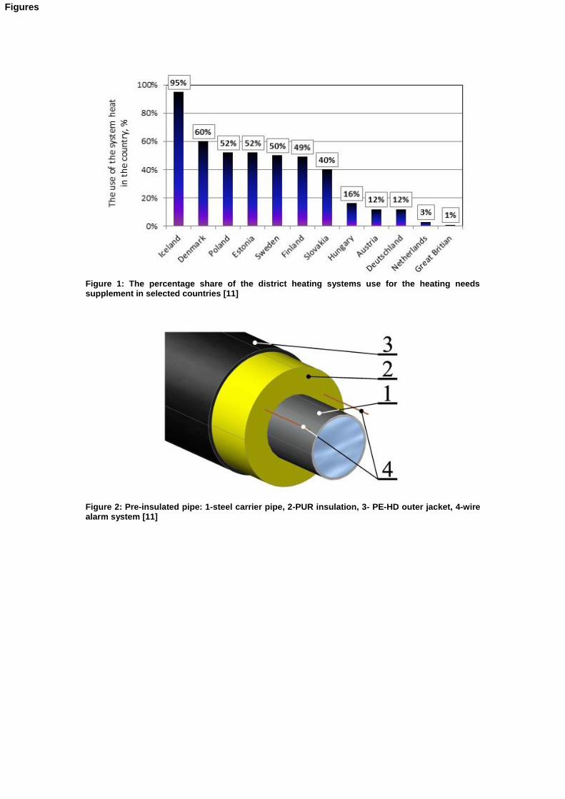
Figure 1: The percentage share of the district heating systems use for the heating needs supplement in selected countries [11]

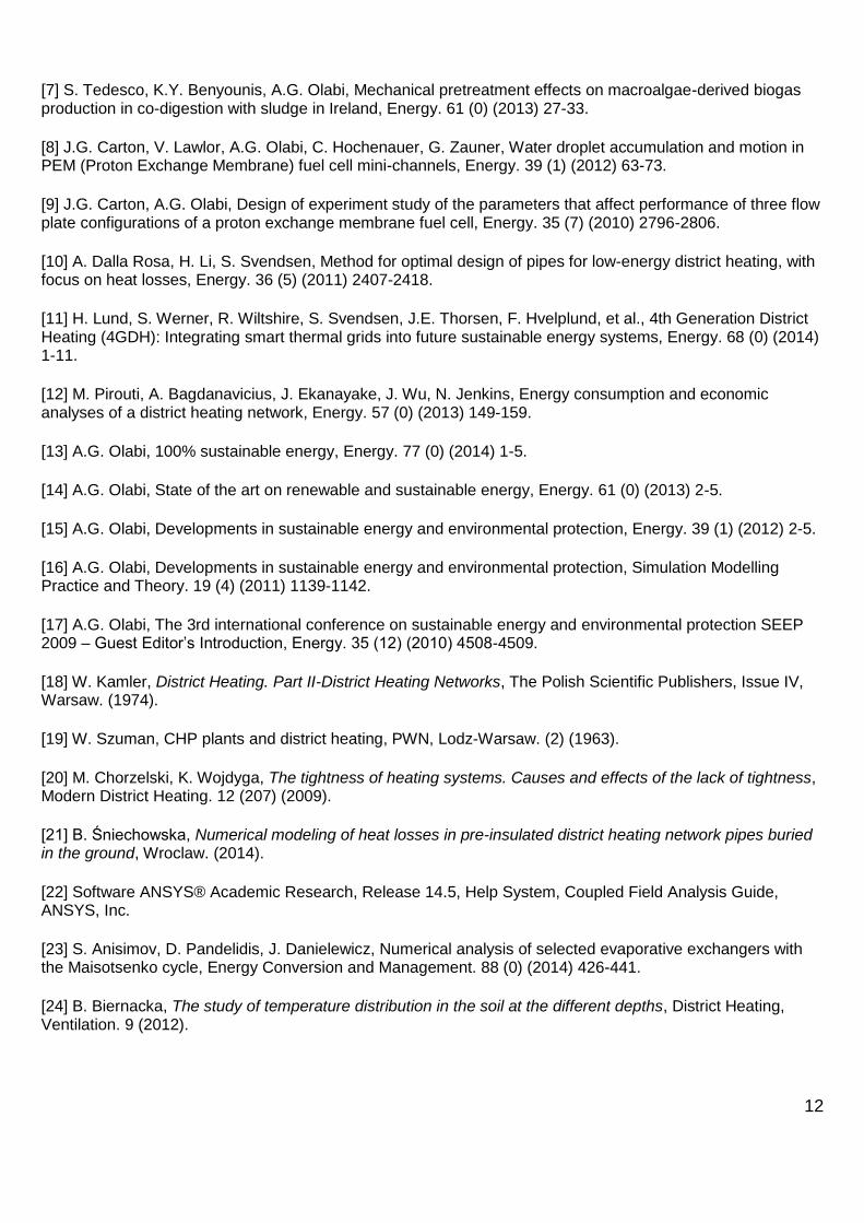
Figure 2: Pre-insulated pipe: 1-steel carrier pipe, 2-PUR insulation, 3- PE-HD outer jacket, 4-wire alarm system [11]

Figures

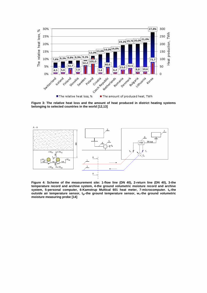
Figure 3: The relative heat loss and the amount of heat produced in district heating systems belonging to selected countries in the world [12,13]

Figure 4: Scheme of the measurement site: 1-flow line (DN 40), 2-return line (DN 40), 3-the temperature record and archive system, 4-the ground volumetric moisture record and archive system, 5-personal computer, 6-Kamstrup Multical 601 heat meter, 7-microcomputer. to-the outside air temperature sensor, tgr-the ground temperature sensor, wv-the ground volumetric moisture measuring probe [14]

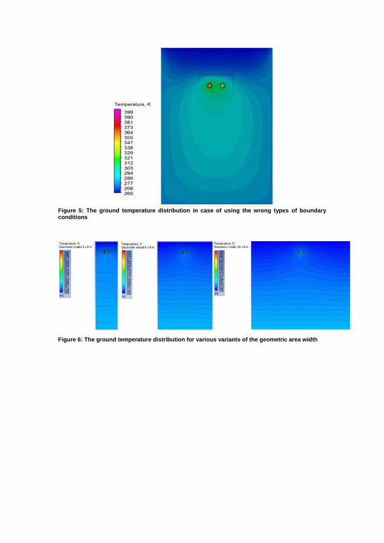
Figure 5: The ground temperature distribution in case of using the wrong types of boundary conditions

Figure 6: The ground temperature distribution for various variants of the geometric area width

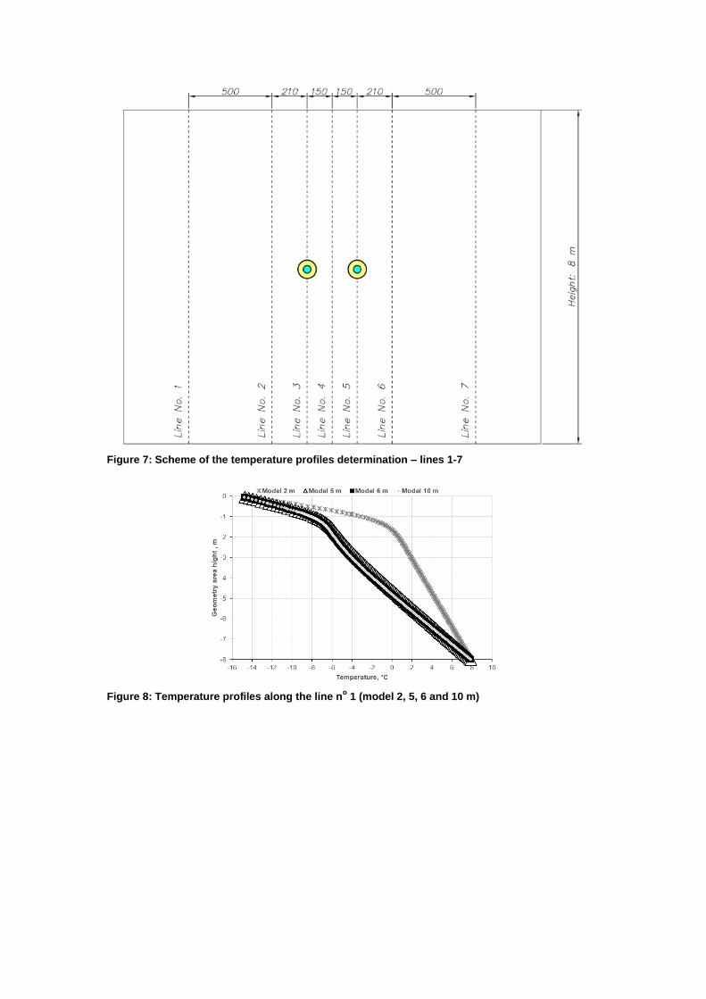
Figure 7: Scheme of the temperature profiles determination – lines 1-7

Figure 8: Temperature profiles along the line n

o 1 (model 2, 5, 6 and 10 m)

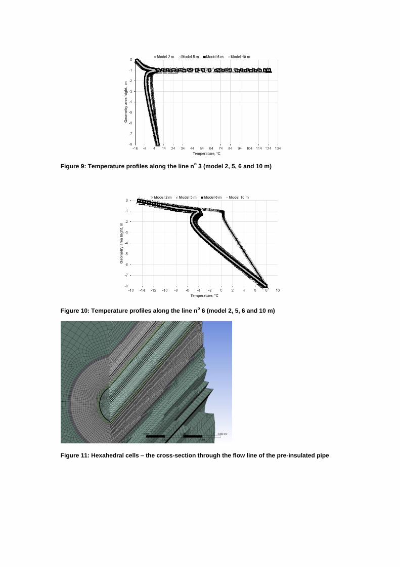
Figure 9: Temperature profiles along the line n

o 3 (model 2, 5, 6 and 10 m)

Figure 10: Temperature profiles along the line n

o 6 (model 2, 5, 6 and 10 m)

Figure 11: Hexahedral cells – the cross-section through the flow line of the pre-insulated pipe

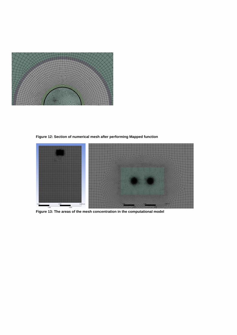
Figure 12: Section of numerical mesh after performing Mapped function

Figure 13: The areas of the mesh concentration in the computational model

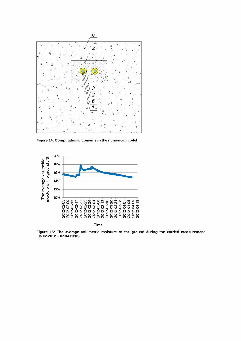
Figure 14: Computational domains in the numerical model

Figure 15: The average volumetric moisture of the ground during the carried measurement (05.02.2012 – 07.04.2012)

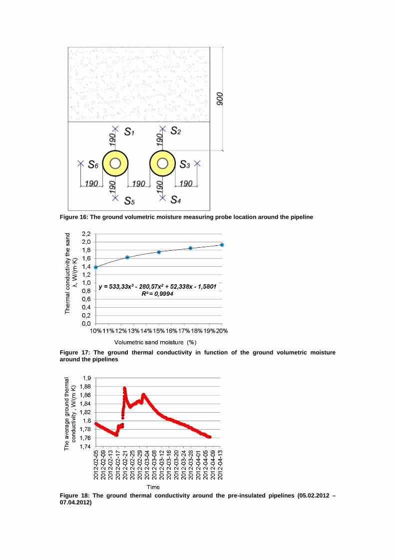
Figure 16: The ground volumetric moisture measuring probe location around the pipeline

Figure 17: The ground thermal conductivity in function of the ground volumetric moisture around the pipelines

Figure 18: The ground thermal conductivity around the pre-insulated pipelines (05.02.2012 – 07.04.2012)

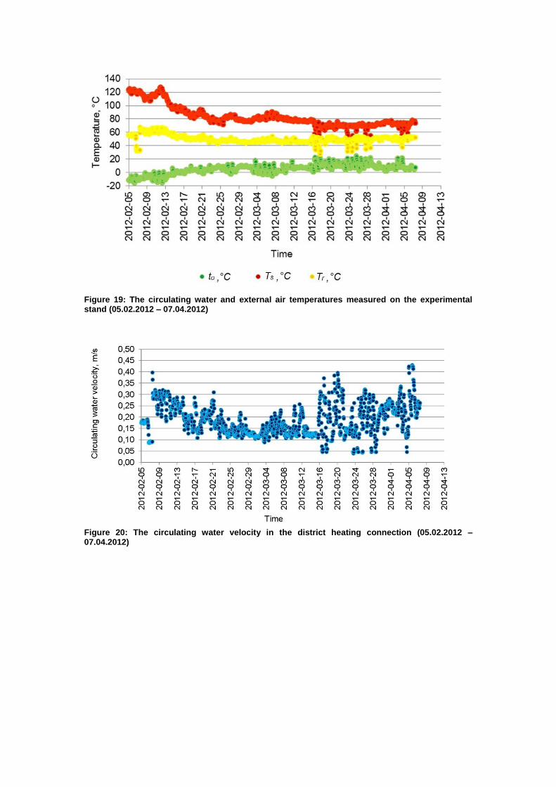
Figure 19: The circulating water and external air temperatures measured on the experimental stand (05.02.2012 – 07.04.2012)

Figure 20: The circulating water velocity in the district heating connection (05.02.2012 – 07.04.2012)

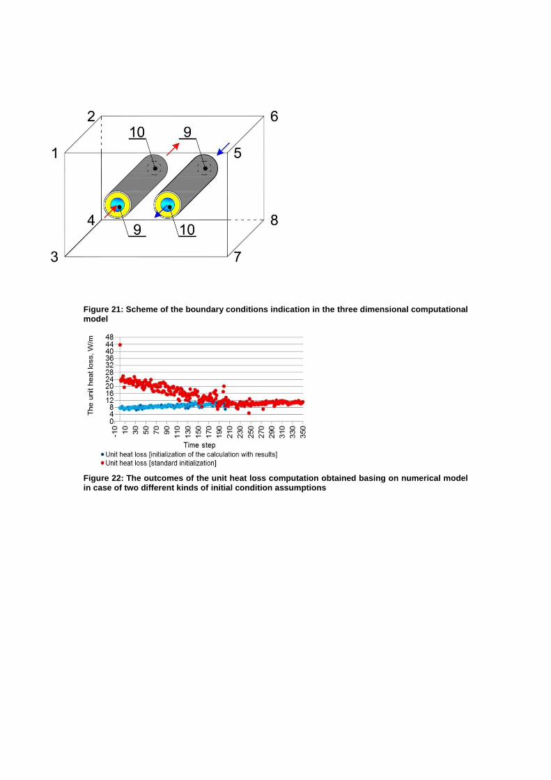
Figure 21: Scheme of the boundary conditions indication in the three dimensional computational model

Figure 22: The outcomes of the unit heat loss computation obtained basing on numerical model in case of two different kinds of initial condition assumptions

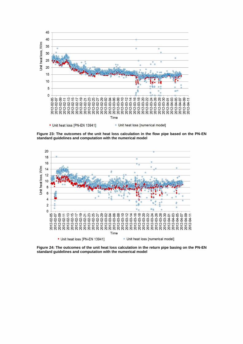
Figure 23: The outcomes of the unit heat loss calculation in the flow pipe based on the PN-EN standard guidelines and computation with the numerical model

Figure 24: The outcomes of the unit heat loss calculation in the return pipe basing on the PN-EN standard guidelines and computation with the numerical model

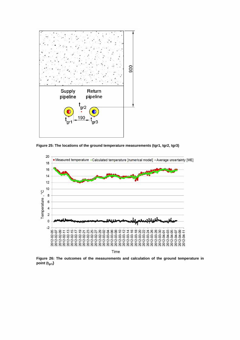
Figure 25: The locations of the ground temperature measurements (tgr1, tgr2, tgr3)

Figure 26: The outcomes of the measurements and calculation of the ground temperature in

point (tgr1)

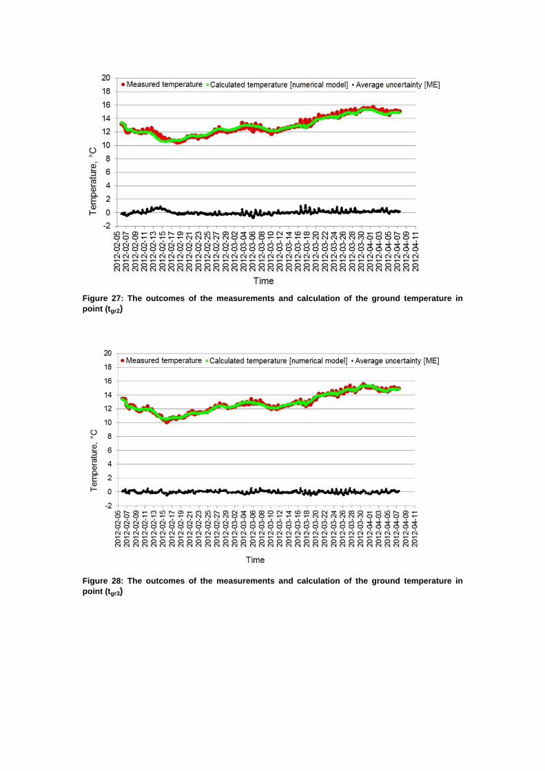
Figure 27: The outcomes of the measurements and calculation of the ground temperature in

point (tgr2)

Figure 28: The outcomes of the measurements and calculation of the ground temperature in

point (tgr3)

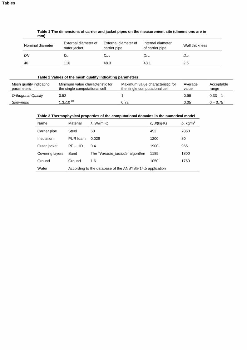
Table 1 The dimensions of carrier and jacket pipes on the measurement site (dimensions are in mm)

Nominal diameter External diameter of

outer jacket

External diameter of

carrier pipe

Internal diameter

of carrier pipe Wall thickness

DN Do Dout Dinn Dwt

40 110 48.3 43.1 2.6

Table 2 Values of the mesh quality indicating parameters

Mesh quality indicating parameters

Minimum value characteristic for the single computational cell

Maximum value characteristic for the single computational cell

Average value

Acceptable range

Orthogonal Quality 0.52 1 0.99 0.33 – 1

Skewness 1.3x10-10

0.72 0.05 0 – 0.75

Table 3 Thermophysical properties of the computational domains in the numerical model

Name Material λ, W/(m·K) c, J/(kg·K) ρ, kg/m3

Carrier pipe Steel 60 452 7860

Insulation PUR foam 0.029 1200 80

Outer jacket PE – HD 0.4 1900 965

Covering layers Sand The “Variable_lambda” algorithm 1185 1800

Ground Ground 1.6 1050 1760

Water According to the database of the ANSYS® 14.5 application

Tables