HAL Id: tel-01130838https://pastel.archives-ouvertes.fr/tel-01130838

Submitted on 12 Mar 2015

HAL is a multi-disciplinary open accessarchive for the deposit and dissemination of sci-entific research documents, whether they are pub-lished or not. The documents may come fromteaching and research institutions in France orabroad, or from public or private research centers.

L’archive ouverte pluridisciplinaire HAL, estdestinée au dépôt et à la diffusion de documentsscientifiques de niveau recherche, publiés ou non,émanant des établissements d’enseignement et derecherche français ou étrangers, des laboratoirespublics ou privés.

Three Essays on Financial InnovationBoris Vallée

To cite this version:Boris Vallée. Three Essays on Financial Innovation. Business administration. HEC, 2014. English.�NNT : 2014EHEC0008�. �tel-01130838�

! ! ! !! !! ! !

ECOLE%DES%HAUTES%ETUDES%COMMERCIALES%DE%PARIS%Ecole%Doctorale%«%Sciences%du%Management/GODI%»%B%ED%533%

Gestion%Organisation%%Décision%Information%

"Three%Essays%on%Financial%Innovation.”%THESE%

présentée%et%soutenue%publiquement%le%25%juin%2014%en%vue%de%l’obtention%du%

DOCTORAT%EN%SCIENCES%DE%GESTION%Par%

Boris%VALLEE%

JURY%

Président%du%Jury%:% % Monsieur%Marcin%KACPERCZYK%Professeur%Imperial%College,%Londres%–%UK%

%%Directeur%de%Recherche%: Monsieur%Ulrich%HEGE%%%% % % % Professeur%% % % % HEC%%Paris%–%France%%CoBDirecteur%de%Recherche%: % Monsieur%Christophe%PERIGNON%%%% % % % Professeur%Associé,%HDR%% % % % HEC%%Paris%–%France%%% % % % %Rapporteurs%: Monsieur%JeanBCharles%ROCHET%% % % % Professeur%

Université%de%Zurich%–%Suisse%%Madame%Paola%Sapienza%!

% % % % Professeur%%%% % % % Kellogg%School%of%Management,%%

Northwestern%University,%Illinois%–%USA%%% % % % %Suffragants%: Monsieur%Laurent%CALVET%

Professeur%HEC%%Paris%–%France%

% % % %Monsieur%Guillaume%PLANTIN%

% % % % Professeur%%Université%de%Toulouse%Capitole%1–%France%%%Monsieur%David%THESMAR%Professeur,%HDR%HEC%%Paris%–%France%

%%

%%%%%%%%%%%%%%%%%%

% %

%%%

Ecole%des%Hautes%Etudes%Commerciales%

Le%Groupe%HEC%Paris%n’entend%donner%aucune%approbation%ni%improbation%aux%%

opinions%émises%dans%les%thèses%;%ces%opinions%doivent%être%considérées%%

comme%propres%à%leurs%auteurs.%

Three Essays on Financial

Innovation

Ph.D. dissertation submitted by:

Boris Vallee

Committee Members:

Advisors:

Laurent Calvet

Ulrich Hege, Research Director

Christophe Perignon, Co-Director

David Thesmar

External Members:

Marcin Kacperczyk (Imperial College)

Guillaume Plantin (Toulouse School of Economics)

Jean-Charles Rochet (University of Zurich)

Paola Sapienza (Northwestern University)

To Anna

ii

Acknowledgements

It is not so much our friends’ help that helps us as the confident knowledge that they will

help us. (Epicurus)

Writing this dissertation has been a tremendous educational experience and a reward-

ing chapter in my professional development. This success would by no mean have been

possible without the help and support of all the people around me during these five years,

both in my professional and personal sphere. Now is the time to thank them!

First let me thank the members of my committee, who greatly contributed to the suc-

cess of this dissertation. I am forever endebted to Ulrich Hege for his attentive guidance

and encouragements, and for advising me to do a Ph.D. in the first place. I am deeply

thankful to David Thesmar, who was always available and helped me raise the bar every

time we met. I warmly thank Laurent Calvet for his help and advice, and look forward to

working on our future common project. Last but not least, I am grateful to Christophe

Perignon for educating me about how the academic world works.

I am thankful to Marcin Kasperczyk, Guillaume Plantin, Jean-Charles Rochet and

Paola Sapienza for accepting to take part in my dissertation committee. I look forward to

hearing their feedback and hope to continue having fruitful exchanges with them in the

future. I am grateful to all the members of the Finance department at HEC Paris for their

generous feedback (with a special thank you to Thierry Foucault and Johan Hombert),

and to Josh Rauh and Manju Puri for welcoming me at Northwestern University and

Duke University. I enjoyed the companionship of my fellow Ph.D. candidates along the

five years in HEC: Michael, Hedi, Olivier, Jerome, Jean-Noel, Adrien and Alina, to name

only a few. I will miss our tiny o�ce and discussions! I also thank the HEC Foundation

for funding my scholarship, Lexifi and Jean-Marc Eber for his interest in my research,

and Europlace and IFSID for their research grant.

I also want to warmly thank Claire Celerier, my friend and co-author, for our pro-

iii

ductive collaboration that played a key role in the success of my PhD. Two papers so far

and counting!

My most sincere gratitude goes to my family, who instilled in me a love of knowledge

and a penchant for analytical thought: my parents Anne-Marie and Serge, my sister

Axelle, and my brother Gildas. I also thank my friends, who sometimes teased me, of-

ten helped me, and always encouraged me: Antoine, Clement, Fabrice, Francois, Julien,

Vanessa and Vince, to name only a few.

I dedicate this thesis to Anna, who brought a superior meaning to my visiting schol-

arship in Chicago, and to all the e↵orts made in general.

Thank you everyone!

iv

Introduction

I cannot understand why people are frightened of new ideas. I’m frightened of the old

ones. [John Cage, Composer]

Innovation is the introduction and development of new ideas, devices or methods.

As in other fields, innovation in finance has been questioned on whether it represents

progress. Warren Bu↵et, in the Berkshire Hathaway annual report for 2002, famously

declared: ”Derivatives are financial weapons of mass destruction.” Analyzing both the

motives and e↵ects of financial innovation is key for gaining a better understanding of its

role in our society, and whether financial innovation can help improving welfare (Allen

(2011)).

Financial innovation has been a fundamental companion of economic development

over the centuries, under many di↵erent forms. The introduction of new payment meth-

ods (from the invention of coins in the seventh century BC, to mobile phone payment

in the 21st century), new asset classes (from stocks to cat bonds or Exchange Traded

Funds), new services (from the deposit bank in the 16th century to online banking and

crowdfunding), new processes (credit scoring, asset structuring and pricing), or new play-

ers (Venture Capital, Shadow banks, Hedge Funds) have fundamentally changed the role

and the scope of the finance sector. These innovations have therefore had a profound

impact on our economies and societies. The invention of currency, for instance, led to

the development of cities and the division of labor in the Mesopotamia of the 7th century

before JC. In 13th century China, economy and war funding was eased by the inven-

tion of paper money, or banknotes. The invention of banks allowed the development of

v

Florence and Genova during the 17th century. More recently, micro-credit, invented by

Peace Nobel Laureate Mohammed Yunus, has made it possible for millions of people to

borrow and develop an economic activity.

Despite these examples, the strict identification of financial innovation presents a chal-

lenge, as patents are almost non-existent in an industry that works on an intangible good:

money. It is di�cult to measure to what extent a new type of contract or idea corre-

sponds to a breakthrough or merely represents a marginal change. Despite this challenge,

academics have pointed to an acceleration of financial innovation in the last decades and

have subsequently sought to understand its impact. Tufano (2003) identifies the intro-

duction of 1,836 distinct financial assets from 1980 to 2001. These introductions have

come with a general suspicion towards financial innovation since the 2008 financial crisis.

Innovative financial instruments such as Credit Default Swaps or mortgages securitization

have indeed been pointed out as one of the main drivers of the crisis. More generally,

the utility of financial innovation is being questioned, as illustrated by Paul Volcker’s fa-

mous quote in 2009: “The only thing useful banks have invented in 20 years is the ATM.”

Empirically Investigating Financial Innovation

My dissertation studies recent episodes of financial innovation, with the ambition of

understanding their motives and e↵ects. This research thread has led me to go beyond

the methods and insights of a single subfield of finance, and to relate methods of cor-

porate finance and banking with other fields including household finance, public finance,

political economy, and industrial organization. Generally, no readily available datasets

existed that allowed me to analyze the considered innovative financial products, so in

each chapter the research design involves the construction of new datasets and of original

variables measuring the scope and use of innovation.

Financial Complexity

vi

A frequently debated consequence of financial innovation is the increasing complexity of

financial instruments. Financial complexity may be used as a strategic tool by firms to

increase search costs (Carlin (2009)), or to intentionally reset investors’ learning (Carlin

and Manso (2011)). This chapter, entitled What Drives Financial Complexity? A Look

into the Retail Market for Structured Products, empirically investigates these theoreti-

cal insights on financial complexity in a competitive environment. Claire Celerier and

I focus on the highly innovative retail market for structured products. We perform a

lexicographic analysis of the term sheets of 55,000 retail structured products issued in

Europe since 2002 and construct three indexes measuring complexity. These measures al-

low us to observe that financial complexity has been steadily increasing, even during and

after the recent financial crisis. We show that financial complexity is most prominently

used by banks with the least sophisticated client base, and provide empirical evidence

that intermediaries strategically use complexity to mitigate competitive pressure. First,

complex products exhibit higher mark-ups and lower ex post performance than simpler

products. Second, using issuance level data spanning 15 countries over the 2002-2010

period, we find that financial complexity increases when competition intensifies.

Innovative Borrowing Instruments in Public Finance

In 2001, to comply with Eurozone requirements, Greece entered into an OTC cross-

currency swap transaction to hide a significant amount of its debt. In the chapter entitled

Political Incentives and Financial Innovation: The Strategic Use of Toxic Loans by Local

Authorities, Christophe Perignon and I evidence the use of another form of hidden public

debt by local governments: toxic loans. Using proprietary data, we show that politicians

strategically use these products to increase chances of being re-elected. Consistent with

greater incentives to hide the actual cost of debt, toxic loans are utilized at a signifi-

cantly higher frequency within highly indebted local governments. Incumbent politicians

from politically contested areas are also more likely to turn to toxic loans. Using a

di↵erence-in-di↵erences methodology, we show that politicians time the election cycle by

vii

implementing more transactions immediately before an election than after. Politicians

are also found to exhibit herding behavior in this process. Our findings for the market of

municipal financial products o↵er an example of a strategic use of financial innovation.

Financial Institutions and Contingent Capital

As part of the debate on bank leverage, Bolton and Samama (2012) propose an innova-

tive solution to decrease financial distress costs associated with high leverage of financial

institutions: Contingent Capital with an Option to Convert. In a third chapter entitled

Call Me Maybe? The E↵ects of Exercising Contingent Capital, I study the market reac-

tion and economic performance following the exercise of comparable contingent capital

options embedded in bank capital instruments. During the financial crisis, European

banks massively triggered option features of hybrid bonds they had issued in response

to regulatory capital requirements in order to reduce their debt burden. This episode

constitutes the first ”real-world” experiment of the use of contingent capital features. I

find that these trigger events are positively received by credit markets, while stockholders

discriminate according to the type of resulting debt relief and the financial institution

leverage. Moreover, I document that banks that obtain regulatory debt relief by using the

embedded trigger option exhibit higher economic performance than similar banks that do

not. These findings point to the possible constructive role of innovative debt instruments

as an e↵ective solution to the dilemma of bank capital regulation.

viii

Introduction (En Francais)

Chapitre I

La complexite des produits financiers o↵erts aux menages a augmente de facon spec-

taculaire au cours des vingt dernieres annees. Des produits innovants ont ete developpes

pour l’actif et le passif -par exemple les fonds communs de placement, les cartes de credit

et les prets immobilier, bien que la sophistication financiere des menages reste faible

(Lusardi and Tufano (2009b), Lusardi et al. (2010)). Y a-t-il une tendance actuelle a

l’augmentation de la complexite financiere des produits de detail? Le cas echeant, quelles

sont les raisons de cette augmentation?

Pour repondre a ces questions, nous nous concentrons sur un marche specifique qui a

connu une forte croissance dans la derniere decennie: le marche des produits structures

pour particuliers. Nous developpons un indice de la complexite de ces produits, que nous

appliquons a une base de donnees couvrant 55.000 produits structures pour particuliers

vendus en Europe. A l’aide de cet indice, nous observons que la complexite financiere

a augmente au fil du temps. Nous etudions plusieurs explications d’un point de vue

de la demande pour ce fait stylise: une evolution des besoins et des preferences, une

tendance a un plus grand partage des risques au sein des marches financiers, et un motif

de ”lotterie”. Nos observations ne corroborent que peu ces explications. Nous nous

concentrons donc sur des explications du cote de l’o↵re, en particulier sur l’utilisation

strategique de la complexite qui a ete recemment etudiee theoriquement (par exemple,

Carlin (2009) et Carlin and Manso (2011)) et en organisation industrielle (Ellison (2005)

ix

et Gabaix and Laibson (2006)). Nous trouvons des preuves coherentes avec les predictions

theoriques des modeles supposant une intention d’augmentation des couts de recherche ou

de discrimination par les prix. Tout d’abord, nous montrons que la complexite elevee des

produits est associee a une plus grande rentabilite pour les banques, et des performances

plus faibles pour les investisseurs. Deuxiemement, en utilisant des donnees d’emissions

couvrant 15 pays sur la periode 2002-2010, nous constatons que la complexite des produits

financiers augmente lorsque la concurrence s’intensifie. Notre papier fournit le premier

test empirique de la relation positive entre concurrence accrue et complexite croissante

sur les marches financiers, qui a ete identifiee dans la litterature theorique (Carlin (2009)).

Le premier objectif de cette etude est de mesurer l’augmentation de la complexite

financiere aussi precisement que possible. Nous observons une tendance a l’augmentation

de la complexite financiere en examinant les prospectus de tous les produits structures

pour particuliers emis en Europe depuis 2002 a l’aide d’une analyse textuelle. Nous con-

statons que cette tendance haussiere se poursuit meme apres la crise financiere. Mesurer

la complexite des produits d’une maniere precise et pertinente sur le marche tres diver-

sifie des produits structures pour particuliers represente le premier defi de notre analyse

empirique. Pour ce faire, nous developpons un algorithme qui balaie pour chaque pro-

duit la description du calcul des flux, et identifie les caracteristiques de ces formules.

Nous definissons le niveau de complexite d’un produit donne comme le nombre des car-

acteristiques definissant cette formule. La logique de notre approche est que plus une

formule comprend de caracteristiques distinctes, plus elle est di�cile a comprendre et a

comparer pour l’investisseur. Nous utilisons aussi le nombre de caracteres utilises dans

la description de la formule des flux, ainsi que le nombre de scenarios possibles, comme

des tests de robustesse de notre mesure de complexite. L’observation de la hausse de la

complexite au fil du temps est commune a ces trois mesures de complexite.

Le deuxieme objectif de l’etude est d’explorer les explications possibles de cette com-

plexite croissante dans le marche des produits structures pour particuliers. Nous com-

mencons par explorer les raisons du cote de la demande. Tout d’abord, nous envisageons

x

que cette hausse puisse provenir de l’evolution des preferences ou des besoins des con-

sommateurs. Cependant, nous constatons qu’aucune des nombreuses variables et des

controles que nous utilisons dans notre analyse ne detecte de changements dans la com-

position du marche des produits structures. Deuxiemement, nous analysons si la hausse

de la complexite financiere peut etre liee a l’augmentation de la completude du marche

ou a un meilleur partage des risques. Cependant, cette hypothese devrait impliquer

que la complexite est plus repandue parmi les produits pour investisseurs avertis et for-

tunes, qui devraient obtenir le plus grand avantage de ces opportunites. Cependant, nos

donnees indiquent le contraire: les institutions qui ciblent les clients moins sophistiques,

comme les caisses d’epargne, o↵rent des produits plus complexes. En outre, certaines

caracteristiques specifiques - par exemple, la monetisation d’un plafond sur la hausse de

l’indice sous-jacent - et la monetisation de la possibilite de subir une perte si l’indice

sous-jacent tombe en dessous d’un certain seuil - sont plus frequents lorsque la volatilite

implicite est elevee, ce qui est di�cile a expliquer par des facteurs de demande. En e↵et,

l’aversion au risque des investisseurs est plus faible lors des periodes de crise.

Par consequent, dans notre tentative de comprehension de la hausse de la com-

plexite, nous nous tournons vers des hypotheses d’utilisation strategique de celle-ci. Nous

testons en particulier deux hypotheses decoulant directement de predictions theoriques:

la rentabilite des produits complexes doit etre relativement elevee et la complexite devrait

augmenter lorsque la concurrence s’intensifie. Nous etablissons d’abord une relation entre

la complexite financiere et la rentabilite des produits. Nous calculons la marge realisee

pour un sous-ensemble homogene en terme d’actif sous-jacent de produits structures pour

particuliers, a l’aide d’une methodologie Least Square Monte Carlo. Nous contrastons

ensuite le niveau de rentabilite avec celui de complexite du produit. Nous constatons que

plus un produit est complexe, plus il est rentable. Base sur la performance realisee de 48

% des produits qui sont arrives a terme, nous montrons egalement que plus un produit

est complexe, plus sa performance finale est faible. Deuxiemement, nous etudions em-

piriquement l’e↵et d’un choc de concurrence sur la complexite financiere. Nous utilisons

xi

une methodologie de di↵erence de di↵erences afin d’evaluer l’impact de l’entree des Ex-

change Traded Funds (ETF) sur la complexite des produits structures pour particuliers.

Ce choc a ete utilise par Sun (2014) aux Etats-Unis pour etudier l’impact de la concur-

rence sur les frais des fonds de placement communs. L’entree des ETF represente en e↵et

une augmentation de la concurrence pour les produits structures pour particuliers, car ils

representent un substitut possible a ces produits. Nous constatons que le meme distribu-

teur propose des produits plus complexes dans les pays ou les ETF ont ete introduits que

dans les pays ou ils n’ont pas ete introduits. Nous evaluons egalement l’impact du nombre

de concurrents dans le marche des produits structures pour particuliers sur la complexite

moyenne, explorant ainsi une autre dimension de concurrence. Nous montrons que la

complexite moyenne de l’o↵re de produits du meme distributeur est plus elevee dans les

marches ou le nombre de concurrents a augmente. Ce resultat est robuste au controle

par le niveau de rentabilite du secteur financier au niveau national.

Pour notre etude, nous utilisons une nouvelle base de donnees qui contient des infor-

mations detaillees sur tous les produits structures pour particuliers qui ont ete vendus

en Europe de 2002 a 2011. Cette base de donnees presente des caracteristiques cles qui

facilitent l’analyse textuelle, ainsi que la strategie d’identification propre a une etude

d’organisation industrielle empirique. Elle couvre 17 pays, 9 ans de donnees et plus de

400 concurrents. Pour chaque emission, une description detaillee de la formule de calcul

de performance, de nombreuses autres informations sur le produit et son distributeur,

ainsi que le volume vendu, sont disponibles.

En termes d’implications reglementaires, notre travail souligne la necessite d’evaluer

la complexite des produits independamment de leur risque. Une etape supplementaire

pourrait etre d’imposer un plafond sur la complexite, ou de favoriser la standardisation

des produits financiers pour particuliers afin de limiter la dynamique de complexification

que nous observons. Ces mesures supposent pour le regulateur de developper et d’utiliser

une mesure globale et homogene de la complexite des produits.

xii

Chapitre II

L’innovation financiere vise a ameliorer le partage des risques en parvenant a la

completude des marches financiers. Cependant, les innovations financieres peuvent etre

utilisees a d’autres fins, notamment par les politiciens soucieux de leurs propres interets.

Ainsi, en 2001, afin de se conformer aux exigences de la zone euro, la Grece a mis en

place une transaction de swap de devises de gre a gre avec Goldman Sachs dans le but

de cacher une part importante de sa dette. Aux Etats-Unis, les municipalites utilisent

regulierement une forme de remboursement anticipe qui leur fournit une amelioration

budgetaire a court terme, mais a un cout total eleve ((Ang et al., 2013)).

L’innovation financiere facilite-t-elle les strategies personnelles des politiciens aux frais

du contribuable? Pour repondre a cette question, nous etudions l’utilisation de produits

financiers innovants par les collectivites locales. Nous nous concentrons sur un type de

pret structures, surnommes emprunts toxiques par la presse en raison de leur profil a

haut risque ((Erel et al., 2013). Nous emettons l’hypothese que ces produits sont utilises

comme leviers de strategies deliberees de la part des elus. Comme les utilisateurs de

prets immobiliers complexes etudies par Amromin et al. (2013), les politiciens exploitent-

ils deliberement certaines caracteristiques de ces prets a leur propre avantage, malgre les

risques a long terme encourus?

Pour tester empiriquement cette hypothese, nous exploitons une base de donnees

unique qui inclut les portefeuilles d’emprunts toxiques de pres de 3000 collectivites locales

francaises. En utilisant des analyses transversales et une methodologie de di↵erence des

di↵erences, nous montrons que les politiciens utilisent ces produits plus frequemment et

dans une large mesure lorsque leurs incitations pour cacher le cout de la dette est eleve,

lorsque ils sont les elus d’une zone sujette a l’alternance, et lorsque leur confreres mettent

en œuvre des operations similaires.

Au cours de la recente crise financiere, du fait de la hausse de la volatilite, les frais

d’interet des utilisateurs de prets toxiques ont atteint des niveaux tres eleves. Un exemple

xiii

interessant est la ville de Saint-Etienne, qui poursuit actuellement en justice ses banques

pour avoir vendu des produits financiers accuses d’etre trop risque. En 2010, le taux

d’interet annuel facture sur l’un de ses principaux prets a augmente de 4 % a 24 %,

car il etait indexe sur le taux de change livre / franc suisse (Business Week, 2010). Les

moins-values latentes totales de Saint-Etienne sur les emprunts toxiques ont atteint 120

millions d’euros en 2009, soit presque le niveau de la dette nominale de cette ville : 125

millions d’euros (Cour des comptes, 2011).

Bien que tres repandu, le phenomene des prets toxiques reste peu etudie academiquement.1

Cette absence de recherche sur le sujet resulte principalement d’un manque de donnees

utilisables. Nous nous appuyons sur deux ensembles de donnees inedits qui se completent

mutuellement. Le premier jeu de donnees contient le portefeuille complet de la dette pour

un echantillon d’environ 300 grandes collectivites locales francaises a fin 2007 pour chaque

instrument de la dette. Il contient le montant nominal, la maturite, le taux du coupon

moyen, le type de produit, de l’indice financier, et le preteur identite. Le deuxieme ensem-

ble de donnees comprend toutes les operations d’emprunts structurees faites par Dexia,

la banque leader sur le marche francais pour les prets aux collectivites locales, entre 2000

et 2009. Cette base de donnees fournit des informations au niveau du pret, y compris

la valeur latente de la transaction, et la date de la transaction. Cette derniere variable

est cruciale pour notre strategie d’identification. Contrairement aux etats financiers des

gouvernements locaux qui ne distinguent pas entre prets structures et pret classique, ces

bases de donnees fournissent des informations detaillees sur les types de prets qui sont

utilises par chaque administration locale.

Nous apportons la preuve empirique de l’utilisation strategique de prets toxiques par

les decideurs publics. Nous commencons par montrer que les prets structures representent

plus de 20% de l’ensemble des encours de dette. Plus de 72% des gouvernements locaux

de notre premier echantillon utilisent des prets structures. Parmi ces prets structures,

40% sont toxiques. Une analyse transversale de nos donnees montre que les elus des

1Capriglione (2014) etudie l’utilisation des instruments derives par les gouvernements locaux italiens.

xiv

gouvernements locaux en di�culte financiere sont nettement plus enclins a se tourner

vers ce type de pret, attestant de leur incitation elevee a cacher le cout reel de la dette

contractee. En e↵et, les gouvernements locaux du quartile superieur du point de vue de

l’endettement sont deux fois plus susceptibles d’avoir des prets toxiques par rapport a

ceux du quartile inferieur. Nous constatons egalement que les politiciens elus dans les

zones a alternance frequente sont plus enclins a utiliser les prets toxiques, ce qui suggere

une motivation de leur part a obtenir des economies a court terme pour se faire reelire.

Nous exploitons egalement la dimension temporelle de nos donnees. Nous identifions

un groupe de traitement dont l’election coıncide avec la periode de notre l’echantillon, par

opposition a un groupe de controle qui n’a pas d’elections pour cette periode (par exemple,

les regions, dont le calendrier electoral di↵ere, et les aeroports, les ports, et les hopitaux,

qui n’ont jamais d’elections). En utilisant une methodologie de di↵erence des di↵erences

sur ces deux groupes, nous constatons que le calendrier des elections joue un role impor-

tant: pour le groupe ayant une election, les transactions sont plus frequentes peu avant

les elections que peu apres. L’utilisation d’emprunts toxiques s’appuie egalement sur un

comportement gregaire : les politiciens sont plus susceptibles de contracter des emprunts

toxiques si leurs voisins l’ont fait recemment. Ce comportement gregaire reduit le risque

de reputation, tout en augmentant la probabilite d’un sauvetage collectif en cas de sce-

nario negatif.

Chapitre III

Le levier excessif des institutions financieres a ete un catalyseur important de la

recente crise financiere, ce qui a conduit les regulateurs et les politiciens a blamer les

regles de capital reglementaire comme responsables du niveau d’endettement atteint par

les grandes institutions financieres en amont de la crise. Le debat sur la reglementation

des fonds propres des banques, cependant, a revele un dilemme fondamental. Comme

preconise par les regulateurs (Rapport de la Commission independante des banques dirige

xv

par Sir John Vickers (2013)) et universitaires (Admati et al. (2011)), une augmenta-

tion significative du montant de capital requis pour les banques represente la reponse

logique au risque de faillite financiere devenu manifeste dans les annees 2007 - 2009,

et aidera a eviter de futurs sauvetages bancaires par les gouvernements. L’application

de ces reglements plus contraignants, cependant, est susceptible d’avoir des e↵ets reels

indesirables tels que la contraction du credit, car les investisseurs sont reticents a fournir

aux banques ces fonds propres supplementaires (Jimenez et al. (2013)). Cette reticence

est partagee par les leaders de l’industrie bancaire (Ackermann (2010)). Par consequent,

les instruments de capital contingent, qui combinent les avantages de la dette et des cap-

itaux propres, et representent une solution possible a ce dilemme, semblent etre une voie

prometteuse (Flannery (2005); Brunnermeier et al. (2009); Kashyap et al. (2008), French

et al. (2010)). En principe, la reduction de la dette et l’amelioration de capitalisation

peuvent egalement etre obtenus par des restructurations de la dette a posteriori, par

exemple a l’aide d’echanges de dettes en actions. Les instruments de capital contingent

peuvent, cependant, etre plus e�cace pour eviter le couteux renflouement des banques

par les Etats, ainsi qu’aider a resoudre les problemes de surendettement (Du�e (2010))

sans encourir de risque de defaut ou de l’echec d’un plan de restructuration de la dette.

La substitution d’une partie du capital reglementaire traditionnel en instrument de cap-

ital contingent pourrait permettre aux banques d’ameliorer leur resilience en limitant les

surcouts lies a l’emission de capital supplementaires.2

Le but de cet article est d’evaluer l’e�cacite des instruments de capital contingent

pour resoudre les situations de detresse financiere des institutions financieres. Plus

precisement, cet article repond aux questions suivantes: lorsque la decision d’exercice

du capital contingent est laissee a l’emetteur, celui-ci l’utilise-t-il cet outil adequatement,

c’est- a -dire en periode de stress? Comment les creanciers et actionnaires reagissent-

ils a ces exercices? Quel est l’impact des exercices d’instrument de capital contingent

2La litterature fournit plusieurs exemples de deviation de Modigliani-Miller tels que: les couts degarantie d’operation par les banques, la sous-evaluation des actions emises en raison de l’asymetrie del’information, et la reaction negative du cours des actions a l’annonce d’une nouvelle emission. Pour plusde details, voir Eckbo et al. (2007).

xvi

sur la performance economique des institutions financieres? La litterature sur l’analyse

theorique des instruments de capital contingent est actuellement en plein essor, avec un

volet important sur les incitations d’exercice et leurs e↵ets (Sundaresan and Wang (2013),

Pennacchi et al. (2011), Martynova and Perotti (2012), Zeng (2012), Flannery (2010)).

Cependant, il n’existe aucune etude empirique sur ce sujet a ma connaissance.

Pour repondre a ces questions, cet article s’appuie sur l’emission d’obligations hybrides

de premiere generation en Europe et l’utilisation massive de leurs possibilites d’exercice

par les institutions financieres europeennes pendant la crise financiere recente. Les instru-

ments de capital contingent sont des hybrides entre dette et fonds propres: ils sont emis

sous forme d’obligations, avec paiements de coupons et echeance stipulee, mais compor-

tent des clauses qui permettent leur conversion discretionnaire ou automatique pendant

les periodes de stress en instruments de capital a maturite illimitee. Le capital contin-

gent est moins cher que le capital traditionnel en raison du bouclier fiscal qu’il procure,

et parce qu’il permet de lever des fonds propres que lorsque cela est necessaire. Ces

instruments limitent donc les couts associes a l’emission d’actions a certains etats de la

nature (Bolton and Samama (2012)). Les obligations dites ”hybrides” sont la premiere

generation d’instruments de fonds propres conditionnels, et sont connus comme des ”Trust

Preferred Securities” (TPS) aux Etats-Unis.

La premiere contribution de cet article est de montrer que les banques europeennes

ont massivement utilises les possibilites d’exercice de leurs obligations hybrides au cours

de la periode 2009 - 2012, a l’aide de deux mecanismes: l’extension de leur maturite, et

des o↵res publiques de rachat a des niveaux inferieur au pair. De nombreux emetteurs

ont etendu la maturite de leurs obligations hybrides, en ne procedant pas a leur rappel

lors de leur premiere date de remboursement possible. Dans mes donnees, je trouve

que les banques europeennes n’ont pas rappele a la premiere date de call un total de

200 milliards d’euros d’obligations hybrides. Ce montant represente 30 pour cent des

obligations hybrides en circulation sur la periode, ou 11 % du capital total des banques

europeennes. Les institutions financieres avec les ratios de capital les plus bas, qui sont

xvii

donc les plus susceptibles de sou↵rir d’une contrainte sur leur capital reglementaire, sont

plus enclines a cette action. Cette constatation minimise la crainte que le caractere

discretionnaire des exercices puisse conduire a des comportements de risk-shifting, puisque

que les institutions financieres ne renoncent pas a la reduction de leur dette comme cela

serait le cas si cette hypothese s’averait valide.

Parmi les emetteurs qui etendent la maturite de leurs obligations hybrides, cer-

tains lancent simultanement une o↵re publique d’achat sur celles-ci. L’o↵re d’achat est

generalement mise en œuvre avec une decote importante, inherente au changement de

maturite du titre super-subordonne. Ces actions combinees permettent a l’institution

financiere d’obtenir la decote comme injection de capital Core Tier 1, car elle correspond

a une plus-value.3 Les investisseurs ont apporte plus de 87 milliards d’euros d’obligations

hybrides a ces o↵res de rachat sur la periode, qui ont permis aux banques d’obtenir 22

milliards d’euros de plus-value, et donc d’injection de capital Core Tier 1.

La deuxieme contribution du papier correspond a l’etude de la reaction des investis-

seurs aux exercices de la contingence. Ces evenements sont accueillis favorablement par

les creanciers, alors que la reaction des actionnaires est plus mitigee. La reaction du

marche est plus prononcee pour les extensions de maturite couplees avec des o↵res de

rachat, ce qui est coherent avec leur e↵et sur le Core Tier 1, un indicateur cle pour le

regulateur pendant la crise. En outre, les o↵res d’echange en actions, qui reduisent le

plus l’endettement, sont recus positivement a la fois par les creanciers et les actionnaires.

La troisieme contribution du chapitre consiste a fournir des preuves empiriques des

e↵ets economiques positifs et persistants pour les banques de l’exercice du capital contin-

gent. Les institutions financieres qui obtiennent un allegement permanent de leur dette

par ce moyen obtiennent un rendement sur actifs plus eleves, et cette amelioration relative

est proportionnelle a l’augmentation des fonds propres Core Tier 1 lors de l’operation.

Cet e↵et est robuste au controle des renflouements des Etats, ainsi que des augmentations

de capital. De plus, l’activite de pret demeure plus soutenue pour ces institutions.

3Le Core Tier 1, ou Common Equity Tier 1, represente la plus haute qualite de capital, et n’inclutpas le goodwill et les instruments hybrides.

xviii

Les extensions de maturite, couplees avec des o↵res de rachat ont des e↵ets economiques

similaires a l’exercice des instruments de capital contingent actuellement emis : Obliga-

tions Write-O↵ et CoCos : un gain en capital immediat, combine dans certains cas a

une emission d’actions. Puisque les regulateurs et les analystes financiers se concentrent

sur le capital reglementaire, l’impact des allegements de la dette sur les ratios de fonds

propres reglementaires est essentiel pour l’emetteur. Le caractere discretionnaire des ex-

ercices etudies dans ce chapitre les rend encore plus comparable a la forme de capital

contingent propose par Bolton and Samama (2012), Capital contingent avec option de

conversion. 4 Par consequent, mes resultats illustrent comment des produits innovants

au passif peuvent aider ex ante a diminuer les couts de detresse financiere associes a un

fort e↵et de levier.

4Ces instruments sont des obligations convertibles en actions, ou la possibilite de convertir appartienta l’emetteur.

1

Contents

1 What Drives Financial Complexity? 5

1.1 Introduction . . . . . . . . . . . . . . . . . . . . . . . . . . . . . . . . . . 7

1.2 The Retail Market for Structured Products . . . . . . . . . . . . . . . . . 11

1.2.1 Background . . . . . . . . . . . . . . . . . . . . . . . . . . . . . . 11

1.2.2 Data . . . . . . . . . . . . . . . . . . . . . . . . . . . . . . . . . . 13

1.3 Measuring Financial Complexity . . . . . . . . . . . . . . . . . . . . . . . 15

1.3.1 Classifying Payo↵s . . . . . . . . . . . . . . . . . . . . . . . . . . 15

1.3.2 Results . . . . . . . . . . . . . . . . . . . . . . . . . . . . . . . . . 16

1.3.3 Robustness Checks . . . . . . . . . . . . . . . . . . . . . . . . . . 17

1.4 Demand-Side Explanations of Financial Complexity . . . . . . . . . . . . 18

1.4.1 Catering to Changing Needs and Preferences . . . . . . . . . . . . 18

1.4.2 Risk Sharing and Increasing Completeness . . . . . . . . . . . . . 19

1.4.3 Gambling Products . . . . . . . . . . . . . . . . . . . . . . . . . . 20

1.5 The Strategic Use of Financial Complexity . . . . . . . . . . . . . . . . . 21

1.5.1 Theoretical Considerations . . . . . . . . . . . . . . . . . . . . . . 21

1.5.2 Financial Complexity and Product Profitability . . . . . . . . . . 23

1.5.3 Complexity and Competition: The impact of ETF entry on com-

plexity . . . . . . . . . . . . . . . . . . . . . . . . . . . . . . . . . 27

1.5.4 Complexity and Competition: Number of Competitors in the Retail

Market for Structured Products . . . . . . . . . . . . . . . . . . . 29

1.6 Conclusion . . . . . . . . . . . . . . . . . . . . . . . . . . . . . . . . . . . 31

2

1.7 Figures and Tables . . . . . . . . . . . . . . . . . . . . . . . . . . . . . . 33

2 Political Incentives and Financial Innovation 49

2.1 Introduction . . . . . . . . . . . . . . . . . . . . . . . . . . . . . . . . . . 51

2.2 The Toxic Loan Market . . . . . . . . . . . . . . . . . . . . . . . . . . . 54

2.2.1 Common Characteristics of Structured Loans . . . . . . . . . . . 54

2.2.2 Which Structured Loans Are Toxic? . . . . . . . . . . . . . . . . . 55

2.2.3 Example of a Toxic Loan . . . . . . . . . . . . . . . . . . . . . . . 56

2.2.4 Local Government Rationale . . . . . . . . . . . . . . . . . . . . . 56

2.2.5 Post-crisis developments . . . . . . . . . . . . . . . . . . . . . . . 57

2.3 Data . . . . . . . . . . . . . . . . . . . . . . . . . . . . . . . . . . . . . . 57

2.3.1 Local Government-Level Data from a Leading Consulting Firm

(Dataset A) . . . . . . . . . . . . . . . . . . . . . . . . . . . . . . 57

2.3.2 Bank-Level Data on Structured Transactions from Dexia (Dataset

B) . . . . . . . . . . . . . . . . . . . . . . . . . . . . . . . . . . . 59

2.4 Empirical Analysis . . . . . . . . . . . . . . . . . . . . . . . . . . . . . . 60

2.4.1 Incentives to Hide the Cost of Debt . . . . . . . . . . . . . . . . . 60

2.4.2 Political Cycle . . . . . . . . . . . . . . . . . . . . . . . . . . . . . 63

2.4.3 Herding . . . . . . . . . . . . . . . . . . . . . . . . . . . . . . . . 65

2.4.4 Political A�liation and Fiscal Policy . . . . . . . . . . . . . . . . 67

2.4.5 Alternative Motive: Hedging . . . . . . . . . . . . . . . . . . . . . 67

2.5 Conclusion . . . . . . . . . . . . . . . . . . . . . . . . . . . . . . . . . . . 68

2.6 Figures and Tables . . . . . . . . . . . . . . . . . . . . . . . . . . . . . . 70

3 Call Me Maybe? 80

3.1 Introduction . . . . . . . . . . . . . . . . . . . . . . . . . . . . . . . . . . 82

3.2 Background and Debt Relief Mechanisms . . . . . . . . . . . . . . . . . . 86

3.2.1 The European Hybrid Bond Market in the Run-up to the Crisis . 86

3.2.2 The Contingent Nature and Regulatory Treatment of Hybrid Bonds 88

3

3.2.3 Contingent Debt Relief Events . . . . . . . . . . . . . . . . . . . . 89

3.3 Data . . . . . . . . . . . . . . . . . . . . . . . . . . . . . . . . . . . . . . 90

3.4 Contingent Debt Relief Use . . . . . . . . . . . . . . . . . . . . . . . . . 91

3.5 Market Reaction to Contingent Debt Relief Events . . . . . . . . . . . . 93

3.5.1 Hypotheses . . . . . . . . . . . . . . . . . . . . . . . . . . . . . . 93

3.5.2 Event Study . . . . . . . . . . . . . . . . . . . . . . . . . . . . . . 95

3.6 Economic E↵ects of Contingent Debt Relief . . . . . . . . . . . . . . . . 99

3.6.1 Impact on Economic Performance . . . . . . . . . . . . . . . . . . 99

3.6.2 Inspecting the Transmission Mechanism . . . . . . . . . . . . . . 100

3.7 Discussion . . . . . . . . . . . . . . . . . . . . . . . . . . . . . . . . . . . 101

3.7.1 Alternative Hypotheses . . . . . . . . . . . . . . . . . . . . . . . . 101

3.7.2 Comparison with Second-Generation Contingent Capital Instruments104

3.7.3 Comparing Europe and the United States . . . . . . . . . . . . . 105

3.8 Conclusion . . . . . . . . . . . . . . . . . . . . . . . . . . . . . . . . . . . 105

3.9 Figures and Tables . . . . . . . . . . . . . . . . . . . . . . . . . . . . . . 107

4 Conclusion 122

5 Appendices 123

Appendix A Chapter 1 . . . . . . . . . . . . . . . . . . . . . . . . 124

Appendix A.1Typology of Retail Structured Products . . . . . . . . . . . 124

Appendix A.2- Figures. . . . . . . . . . . . . . . . . . . . . . . . . 126

Appendix A.3- Tables . . . . . . . . . . . . . . . . . . . . . . . . . 127

Appendix A.4- Theoretical Framework (Model) . . . . . . . . . . . . . . 132

Appendix B Chapter 2 . . . . . . . . . . . . . . . . . . . . . . . . 135

Appendix B.1Types of Structured Debt Products and Risk Classification . . . 135

Appendix B.2Tables . . . . . . . . . . . . . . . . . . . . . . . . . . 138

Appendix C Chapter 3 . . . . . . . . . . . . . . . . . . . . . . . . 140

4

Chapter 1

What Drives Financial Complexity?

A Look into the Retail Market for Structured Products

Joint work with Claire Celerier (University of Zurich)

KISS: Keep It Simple, Stupid.

[US Navy Motto in the 1960s]

6

1.1 Introduction

Abundant anecdotal evidence suggests that the complexity of household financial prod-

ucts has dramatically increased over the last twenty years. Innovative products have been

introduced continuously on the asset and liability sides -for example for mutual funds,

credit cards, and mortgages -while financial literacy and sophistication seem to remain

low (Lusardi and Tufano (2009b), Lusardi et al. (2010)). Is there an actual trend towards

increasing financial complexity in retail products? If so, what drives this increase?

To answer these questions, we focus on a specific market that has been experienc-

ing sustained growth and innovation in the last decade: the retail market for structured

products. We first develop an index of product complexity, which we apply to a compre-

hensive dataset of 55,000 retail structured products sold in Europe. We observe through

this index that financial complexity has been increasing over time. We consider several

demand-side explanations for this stylized fact: catering to changing needs and prefer-

ences, a trend to more risk sharing and better market completeness, and a gambling

motive. Observations from our data do not corroborate the first three explanations.

We therefore focus on supply side based explanations, specifically on the strategic use

of complexity that has been stipulated in various theoretical contributions in finance

(e.g., Carlin (2009) and Carlin and Manso (2011)) and in industrial organization (Ellison

(2005) and Gabaix and Laibson (2006)). We find evidence consistent with the theoretical

explanations that emphasize motives such as increasing search costs or price discrimi-

nation. First, we document that product complexity is associated with higher product

profitability for banks and lower performance for investors. Second, using issuance level

data spanning 15 countries over the period 2002-2010, we find that product financial

complexity increases when competition intensifies. Our paper provides the first empirical

test of the positive relationship between heightened competition and increasing financial

complexity, which has been postulated in the theoretical literature (Carlin (2009)).

The first objective of this paper is to measure the possible increase in financial com-

plexity as accurately as possible. We document a trend of increasing financial complexity

by examining the product term sheets of all the retail structured products issued in Eu-

rope since 2002 through a lexicographic analysis. We find that this trend continues even

after the financial crisis. A major empirical challenge of our analysis lies in measuring

product complexity in an accurate and relevant way in the highly diverse market of retail

structured products. To do so, we develop an algorithm that precisely strips and identifies

each feature embedded in the payo↵ formula of all the past and currently existing struc-

tured products in the retail market. We define the complexity level of a given product

as its total number of features. The rationale of our approach is that the more features

7

a product has, the more complex it is for the investor to understand and compare. We

also use the number of characters used in the pay-o↵ formula description, as well as the

number of potential scenarios, as robustness checks for our measure of complexity. The

finding of increasing financial complexity over time is robust to any of these complexity

measures.

The second objective of the paper is to explore possible explanations for this increas-

ing complexity in the retail market for structured products. We begin by investigating

demand side explanations. First, we examine whether this observation results from cater-

ing to changing preferences or consumer needs. However, we find that none of the many

variables and controls we use detects any time trends or shifts in the composition of

the market for structured products. Second, we analyze whether rising financial com-

plexity is linked to increasing market completeness or better risk sharing opportunities.

However, this hypothesis should imply that complexity is more prevalent among prod-

ucts for sophisticated and a✏uent investors, who should obtain the largest benefit from

such opportunities. However, our data indicate the opposite: institutions that target

unsophisticated clients, such as savings banks, o↵er relatively more complex products.

Additionally, specific product features - e.g., monetizing a cap on the rise of the under-

lying index above a certain threshold - and more surprisingly monetizing the possibility

to take a loss if the underlying index drops below a certain threshold - are more frequent

when implied volatility is high, potentially driving up the average product complexity

during these periods.

Therefore, in our attempt to understand the origins of increasing complexity, we turn

to arguments explaining the use of financial complexity as a strategic tool to mitigate

competitive pressure. Based on ample theoretical literature, we test in particular two

hypotheses: markup of complex products should be relatively higher, and complexity

should increase when competition intensifies. We first establish a relationship between

financial complexity and product profitability. We price a subset of very homogenous

retail structured products based on liquid underlying assets with Least Square Monte

Carlo and then examine the explanatory power of product complexity for markups. We

find that the more complex a product is, the more profitable it becomes. Based on the

realized ex-post performance of 48% of the products that have matured, we also show

that the more complex a product is, the lower its final performance. These findings are

consistent with higher complexity being associated with a higher profit for the distributing

intermediaries. Second, we empirically investigate the e↵ect of a competition shock on

financial complexity. We implement a di↵erence-in-di↵erences methodology to assess the

impact of Exchange Trading Fund (ETF) entries, on complexity. This instrument has

first been used by Sun (2014) in the US to study the price impact of competition on

8

active management investment products. The entry of ETFs represents an increase of

competition for retail structured products, as ETFs can be o↵ered as a substitute to these

products. We find that the same distributor o↵ers more complex products in countries

where ETFs have been introduced than in countries where they have not been introduced.

A specification with bank-year fixed e↵ects further mitigates potential concerns over

reverse causality between ETF entries and financial complexity. We also assess the impact

of the number of competitors in the retail market for structured products on complexity,

thus exploring another dimension of competition. We show that the average complexity

of the product o↵er from the same distributor is higher in markets where the number

of competitors has increased, which is again consistent with distributors adapting to the

competitive environment. This result is robust to controlling for country level financial

sector profitability, which could drive endogenously the number of competitors.

We use a new dataset that contains detailed information on all the retail structured

products that have been sold in Europe since 2002. This database has key characteristics

that facilitate text analysis, as well as a clean identification strategy in an empirical

industrial organization study. It covers 17 countries and 9 years of data, with both strong

inter-country and inter-temporal heterogeneity. It includes more than 300 competitors.

At the issuance level, a detailed description of payo↵s, information on distributors, and

volume sold are available.

There are several reasons to study the financial complexity dynamics in the retail

market for structured products; one of them is the sheer size of the market. In Europe

alone, outstanding volumes of retail structured products add up to more than EUR 700bn,

which is equivalent to 12% of the mutual fund industry. Assets under management have

been steadily growing, despite the financial crisis, with the US market exhibiting USD

160bn of retail structured product issuance since 2010. As direct participation in financial

markets has been structurally decreasing in Europe, structured products often represent a

privileged way of getting exposure to stock markets. In addition, information asymmetry

is high between innovators, investment banks structuring the products, and the final

consumer: the mass-market retail investor. We find many examples of products that

pile up many complex features which are then marketed to savings bank customers, who

are less likely to be sophisticated.1 This finding illustrates the gap between supply-side

complexity and demand-side sophistication. In this study, we define financial complexity

from the investor’s point of view, meaning how di�cult it is for him or her to understand

a product and compare it with possible alternatives.2

1See section 3 for an example.2We do not take the structuring bank point of view: how di�cult it is to create a given product. A

product simple to understand can be challenging to structure. For instance, derivatives on real estate,although easily understood by retail investors are extremely di�cult to structure for banks, mainly for

9

Our work contributes to several fields of the literature. First, our paper builds on

the theoretical literature on financial complexity. Ellison (2005) and Gabaix and Laibson

(2006) describe how ine�cient product complexity emerges in a competitive equilibrium.

To account for the complexity increase in financial products, Carlin (2009) and Carlin

and Manso (2011) develop models in which the fraction of unsophisticated investors is

endogenous and increases with product complexity. Carlin (2009) shows that as compe-

tition intensifies, product complexity increases. Our paper tests direct implications from

these models by empirically assessing the role of competition in the evolution of financial

complexity. Sun (2014) tests empirically the e↵ect of competition on price discrimination

against consumers with low price sensitivity. More specifically, our work contributes to

the emerging field on complex securities (Gri�n et al. (2013), Ghent et al. (2013), Carlin

et al. (2013), Amromin et al. (2011), Sato (2013)).

Our project also complements the literature on the role of financial literacy and limited

cognition in consumer financial choices and bank strategies. Bucks and Pence (2008) and

Bergstresser and Beshears (2010) explore the relationship between cognitive ability and

mortgage choice. Lusardi and Tufano (2009a) find that people with low financial literacy

are more likely to take poor financial decisions. Complexity might amplify these issues.

This paper also relates to the recent interest in the role of financial intermediaries in

providing product recommendations to potentially uninformed consumers (Anagol and

Cole (2013)).

Our paper also adds to the literature on structured products. Hens and Rieger (2008)

theoretically reject completing markets as a motive for complexity by showing that the

most represented structured products do not bring additional utility to investors in a

rational framework. Empirical papers on the retail market for structured products have

focused on the pricing of specific types of products. Henderson and Pearson (2011)

estimate overpricing by banks to be almost 8%, on the basis of a detailed analysis of

64 issues of a popular type of retail structured products. This result challenges the

completeness motive, as it will come at too high a cost.

In terms of policy implications, our work stresses the need to assess product complexity

independently from risk. An additional step may be to impose a cap on complexity or to

foster the standardization of retail structured products to limit the competition dynamics

we observe. Such measures suppose for the regulator to develop and use a comprehensive

and homogenous measure of product complexity beforehand.

Our paper is organized as follows: we begin in section 2 by providing background

information on the retail market for structured products. Our methodology for building

liquidity reasons. The incentive is clear for a structuring bank to be the only one to price a product asit allows charging the monopolistic price.

10

a complexity index is described in section 3, as well as the trend towards increasing

complexity. Section 4 considers possible demand-side explanations for the increase in

financial complexity. Section 5 explores the strategic use of financial complexity. Finally,

section 6 concludes.

1.2 The Retail Market for Structured Products

1.2.1 Background

Retail structured products regroup any investment products marketed to retail investors

with a payo↵ that is determined following a formula defined ex-ante. They leave no

place for discretionary investment decisions along the life of the investment.3 Our study

excludes products with pay-o↵s that are a linear function of a given underlying perfor-

mance, e.g., ETFs. Retail structured products are typically structured with embedded

options. Although these products largely rely on equities, the exposure one can achieve

with them is very broad: commodities, fixed income or other alternative underlyings,

with some example of products even linked to the Soccer World Cup results.

Below is an example of a product commercialized by Banque Postale (French Post

O�ce Bank) in 2010:

Vivango is a 6-year maturity product whose final payo↵ is linked to a basket of

18 shares (largest companies by market capitalization within the Eurostoxx50).

Every year, the average performance of the three best-performing shares in

the basket, compared to their initial levels is recorded. These three shares are

then removed from the basket for subsequent calculations. At maturity, the

product o↵ers guaranteed capital of 100%, plus 70% of the average of these

performances recorded annually throughout the investment period.

This example illustrates the complexity of a popular structured product, which contrasts

with the likely level of financial sophistication of the average client of Banque Postale.

The biased underlying dynamic selection and the averaging of performance across time

makes the product complex to assess in terms of expected performance.

The retail market for structured products has emerged in 1996 and has been steadily

growing from then on. In 2011, assets under management of retail structured products

amount to about 700 billion euros in Europe, which amounts to nearly 3% of all Euro-

pean financial savings, or 12% of mutual funds’ asset under management. Europe, with

3Retail structured product do not give any discretion to the investor in terms of exercising options,which is done automatically, as opposed to mortgages.

11

a market share of 64%, and 357 distributors in 2010 is by far the largest market for

these products. However, the US and Asia are catching are growing quickly. The US

market has met USD160bn of retail structured product issuance since 2010.4 Regulation,

both in terms of consumer protection and bank perimeter is the main explanation for the

di↵erence in size between the European and the US markets. Consumer protection im-

poses retail structured products to have a high minimum investment in the US, typically

USD250,000. Furthermore, the Glass Steagall Act limited internal structuring of these

products until its repeal in 1999. The predominant role of personal brokers as financial

advisers in the US, as opposed to bank employees, may also have played a role.

The growth of this market has been fostered by an increasing demand for passive

products, as the added value of active management has become more and more challenged

(Jensen (1968) or Grinblatt and Titman (1994)). Structured product profitability for the

banks structuring and distributing them also plays an important role (Henderson and

Pearson (2011)). Indeed, on top of disclosed fees, some profits are hidden in the payo↵

structure that is hedged at better conditions than o↵ered to investor. The incentive to

hide markup within the product has been increased in Europe by recent MiFID regulation

that requires distributors to disclose commercial and management fees. In addition,

retail structured products, when packaged as securities or deposits, can o↵er a funding

alternative for banks, and a possible way of transferring some specific risks to retail

investors.5

The organization of the retail market for structured products is largely explained by

the nature of the structuring process. Since these products are very complex to structure,

only large investment banks have the exotic trading platform required to create them.

But no equivalent barriers of scale exist on the distribution side, and distribution channels

are more dispersed. Consequently, entities distributing the products to retail investors

are often, but not necessarily, distinct from investment banks that structure them. These

products have been marketed by a large range of financial institutions, from commercial

banks, savings banks and insurance, to organizations active in wealth management and

private banking. Many providers emphasize in their marketing e↵orts their expertise in

structuring even when they do not actually structure the products, but only select them

and implement a back-to-back transaction with an entity that can manage the market

risk. Therefore, competition is playing out at two levels: between structuring entities,

which sell to distributors, and between distributors, which sell to retail investors. Our

analysis focuses on the latter, as we are interested in the dynamics of financial complexity

in retail markets.4Source: Euromoney Structured Retail Products.5Recent issuances often allow bank to transfer tail risk to retail investors, as product will incur losses

only in case of a strong decrease of the underlying, such as a 30% decrease in the index.

12

The regulatory framework is a key determinant of the development and structure of

this market, in which both bank supervision and investor protection exist. European

national regulators, which are subordinated to a supranational regulator since 2011, the

European Securities and Markets Authority (ESMA), have been increasingly attentive to

protecting retail investors. The European Commission has developed a single Europe-

wide regulatory framework defined by the UCITS Directive. However, until 2010, na-

tional regulators mainly focused on disclosure requirements, which may have amplified

issues of an asymmetric relationship between intermediaries and clients by mandating

information requirements that were too abundant or too technical for clients, such as

backtesting. MiFID regulation introduced client classification and corresponding prod-

ucts appropriateness. Investors are warned when they choose a product deemed unusual

or inappropriate. However, some national regulators appear to mix complexity with risk,

and focus on the latter. For instance, in his latest guidelines about structured products

(REF 2010), the French regulator limits product complexity if and only if investor capital

is at risk.

1.2.2 Data

Our original data stems from a commercial database, called Euromoney Structured Retail

Products, which collects detailed information on all the retail structured products that

have been sold in Europe since the market inception (1996). As no benchmark data source

exists, it is di�cult to determine the exact market coverage of the database. However,

some country-comparisons suggest that the database provides a comprehensive repository

of the industry.6

The retail market for retail structured products is divided into three categories: flow

products, leverage products, and tranche products. We focus on tranche products, which

are non-standardized products with a limited o↵er period, usually 4 to 8 weeks, and a

maturity date. These products have the largest investor base, the highest amount of

assets under management (they stand for 90% of total volumes), the highest average

volumes, and exhibit the largest heterogeneity in terms of pay-o↵s. We therefore exclude

flow products, which are highly standardized and frequently issued products, as they rep-

resent a high number of issuances with very low volumes (sometimes even null).7 We also

exclude leverage products, which are short term and open-ended products. In tranche

6For instance, the coverage on Danish products is 10% larger than that of a hand collected data onthe same market in Jorgensen et al. (2011)

7These products, for instance bonus and discount certificates, are very popular in Germany. Indeed,hundreds of flow products are issued every day and 825,063 of them have been issued from 2002 to 2010.However, their size is only 20,000 Euros on average, against 8.8 million euros for the core market thatwe consider.

13

products, investors typically implement a buy and hold strategy, because there are signif-

icant penalties for exiting before the maturity of the product. As of December 2010, the

total volume (number) of outstanding structured tranche products was respectively EUR

704bn (41,277) in Europe.8 Data are available for 17 countries in Europe, and cumulated

volumes per country since the market inception are given in Table 1.1. Italy, Spain,

Germany, and France dominate the market in terms of volume sold, making up for 60%

of the total. We match this data with additional information on providers (Bankscope

and hand-collected data), market conditions (Datastream) and macro-economic country

variables (World Bank) at the time of issuance.

INSERT TABLE 1.1

Since 2002, the retail market for structured products has seen the emergence of two

major trends: both the volume sold (Figure 1.1) and the number of distributors have

significantly increased (from 144 in 2002 to 357 in 2010), with a slight decrease since the

financial crisis (Table 1.2). The market is divided between commercial banks, private

banks, saving banks and insurance companies, implying a heterogeneous investor base.

INSERT FIGURE 1.1

Table 1.2 provides summary statistics on the underlying type, distributor type, mar-

keting format, volume and design of the products in our dataset. We observe that equity

is the most widespread exposure, either through single shares, basket of shares or equity

indices. Although slightly decreasing over time, the fraction of products with an equity

underlying represent 77% of products from our sample. In terms of format, structured

notes are becoming increasingly popular, as opposed to collateralized fund type product.

This trend is likely to be motivated by banks trying to raise funding through these in-

struments. With the number of products increasing, the average volume per product has

been decreasing over the last ten years. Finally, products where the investor is guaran-

teed to receive at least her initial investment, which were dominant at the beginning of

the period, are becoming less popular and represent around half of the products in the

recent years.

INSERT TABLE 1.28If we include leverage and flow products, the number of outstanding structured products are 406,037

products and volumes are EUR 822bn.

14

1.3 Measuring Financial Complexity

1.3.1 Classifying Payo↵s

This subsection describes how we measure product complexity in the retail market for

structured products. We develop an algorithm that converts the text description of 55,000

potentially unique products into a quantitative measure of complexity in a robust and

replicable manner. This algorithm identifies features embedded in each payo↵ formula

and counts them. The rationale of our approach is that the more features a product has,

the more complex it is for the investor to understand and compare.

We first develop a typology of all the features retail structured products may be

composed of. This typology classifies the features along a tree-like structure. The eight

nodes of the tree represent the steps that an investor may face to understand the final

payo↵ formula of a retail structured product. Only the first node, the main pay-o↵

formula, is compulsory. The following nodes cover facultative features. Example of

features are: reverse convertible, which increases the investor exposition to a negative

performance of the underlying, or Asian option, where the value of the payo↵ depends

on the average price of the underlying asset over a certain period of time. Each one

of the eight nodes of our typology includes on average five features. Therefore, our

methodology covers more than 70,000 combinations of features and hence di↵erentiated

products. Table 1.3 displays the structure of our typology by representing each node of

the tree. We provide the description for each node and definition for each pay-o↵ feature

in the appendix. Our typology covers exhaustively the features that presently exist in

the market.

INSERT TABLE 1.3

In a second stage, an algorithm scans the text description of the final payo↵ formula of

all the 55,000 products and counts the number of features they contain.9 This algorithm

first runs a lexicographic analysis by looking for specific word combinations in the text

description that pinpoint each feature we have defined in our typology. The algorithm

identifies more than 1,500 di↵erent pay-o↵ features combinations in our data. Then we

simply count the number of features to measure complexity. This approach assumes that

all the features defined in our typology are equally complex. Like for any index, the equal

weighting is a simplification, but it avoids subjective weighting biases. Given the depth of

the breakdown we develop, the potential error introduced by equal weighting is probably

a minor concern when compared to indexes built on a small number of components.

9Each formula description has been translated by the data provider, and only contains the necessaryinformation to calculate the performance of the product.

15

Table 1.4 shows how our methodology applies to two existing products. While the first

product is only made of one feature at the compulsory node: Call, the second exhibits

three distinct features: Call, Himalaya, and Asian option, indicating a higher level of

complexity. The length of the product descriptions also appears to be an increasing

function of the number of features.

INSERT TABLE 1.4

Our methodology allows us to identify and measure the complexity of the payo↵

formula of all the past and currently existing retail structured products, but also that of

virtually any new products that might be invented and marketed in the future. A simple

typology based on the final product formula with corresponding levels of complexity would

indeed not have been satisfying given the high diversity we observe. Our methodology

is especially appropriate as far as it allows us to capture the piling up of features we

observe in the market. Furthermore, our algorithm can easily be updated to take into

account future developments of the market. Updating our algorithm only requires adding

a branch to the feature tree when some new features are created.

1.3.2 Results

Figure 1.2 shows the unconditional average complexity of products from our sample by

year. Complexity appears to be an increasing function of time, with almost no decrease

in its growth trend following the financial crisis.

INSERT FIGURE 1.2

To examine this graphical evidence more formally, we regress our complexity measures

on a linear time trend, as well as year fixed e↵ects in a second specification. We control

for a battery of products characteristics, such as underlying type, distributor, format,

country, volume and maturity. Results are shown in Table 1.5. Both specifications

indicate that complexity has been steadily and significantly increasing over time. The

coe�cient of the linear trend is positive and highly significant. Coe�cients on the year

fixed e↵ects are increasing with time.

INSERT TABLE 1.5

Despite the widespread view that the financial crisis has driven down the complexity

of financial instruments, we find that this is not the case for products targeted to retail

investors. This fact points towards product structuring being driven by the supply side

16

of the market, not the demand side.10 This result is robust to the measure of complexity

we use. In section 5 and 6, we explore an industrial organization explanation for this

increase in complexity.

We then look into the evolution of the distribution of complexity. Figure 1.3 plots

the distribution of products from our sample along our complexity index, for three sub-

periods. The increase of complexity is not driven only by a fraction of the distribution of

complexity, but instead increases across all complexity quartiles. Over time, we observe

a decrease in the share of simple products, as well as an increase in the share of the most

complex products. This empirical fact is consistent with banks piling up new features on

existing pay-o↵ combinations.

INSERT FIGURE 1.3

1.3.3 Robustness Checks

As a first robustness check for our measure of complexity, we use the length of the formula

description, measured by the number of characters. Table 1.4 illustrates that the more

complex a product is, the higher the number of words needed to describe its payo↵.

As a second robustness check, we consider the number of di↵erent scenarios that

impact the final return formula. The same product formula can indeed vary depending

on one or several conditions at maturity or along the life of the product. This measure is

close to counting the number of kinks in the final payo↵ curves, as a change of scenario

translates into a point of non-linearity for the pay-o↵ function.11 We quantify the number

of scenarios by identifying conditional subordinating conjunctions such as “if”, “when”

and “whether” in the text description of the payo↵ formula. Overall, we observe a

correlation around 0.6 between our three di↵erent complexity measures, which illustrates

that they are coherent and still complementary.

We observe the same increasing trend over the year when using the length of descrip-

tions or the number of scenarios as a complexity measure. Figure A.0 in the appendix

provides graphical evidence for this result.

We also consider the possibility that a change in regulation, more specifically the

implementation of the MiFID directive on November 1st, 2007, might have led to a

di↵erent methodology for describing pay-o↵s, therefore creating a measurement error.

10The rise in complexity does not appear to be driven by banks providing additional insurance in theproducts. On the contrary, reverse convertible features, that expose investors to downside, are morefrequent after the crisis than before. This increased popularity is likely to relate to a higher volatilitythat increases the value of selling options. We discuss further this point in the next session.

11However this measure also accounts for path dependency that is not captured by the number of kinksof the final pay-o↵ function.

17

Our result are robust to this regulation shock for the following reasons. First, the text

description we use is extracted from the prospectus and translated by our data-provider

based on the same and stable methodology. This description is therefore not impacted by

the requirement of additional disclosures, such as backtesting and warnings. In addition,

the most significant yearly increase in complexity we observe is anterior to this regulatory

change. Finally, we control the time-consistency of the text description by identifying

manually products with identical pay-o↵s features, before and after the MiFID directive

was implemented. We find that payo↵ descriptions remain very similar, and include

around the same number of characters.

1.4 Demand-Side Explanations of Financial Complex-

ity

This section discusses possible explanations for the increase in complexity we observe

that are based on various aspect of the demand side and their possible evolution.

1.4.1 Catering to Changing Needs and Preferences

A first potential explanation for the increase in complexity that we document is that it is

driven by changing consumer preferences or investor needs and a desire of intermediaries

to cater to these varying patterns by o↵ering a di↵erent portfolio of products. If some

product formats or underlying assets require a relatively high complexity, and become

popular for instance for tax e�ciency reasons, a change in the product mix to cater to

such changes could explain the evolution of complexity. Also, assuming that only sophis-

ticated investors use complex products, if unsophisticated investors leave the market, we

would observe a rise in average complexity. These explanations have in common that

they predict a time-varying composition of the portfolio of structured products that are

available and marketed.

Evidence from data goes against this potential explanation. First, as shown in Table

1.5, this trend of increasing complexity is robust to conditioning on format, underlying,

distributor and country fixed e↵ects, as well as maturity changes. Therefore our stylized

fact cannot be explained by hypotheses that imply a time-varying composition of the

market for structured products in terms of product and distributor mix.

Second, volume appears to be a poor predictor of complexity. Total issuance volume

follows a hump shape over our sample period, while complexity has been increasing over

the whole period. Whereas volumes in 2011 are close to the 2006 level, complexity is

significantly higher. Moreover, conditioning on product issuance volume does not remove

18

the significance of the year fixed e↵ects in column 2 of Table 1.5. Also, the decrease in

issuance volume after 2007 is in line with other risky products such as ETFs, and does

not suggest a massive flee from these types of products vs. simpler ones within the risky

financial assets. Overall, change in the composition of the population of retail investors

is likely to be low.

1.4.2 Risk Sharing and Increasing Completeness

A second potential explanation for the increase in complexity is that banks are progres-

sively o↵ering products that better suit retail investor demand for risk sharing oppor-

tunities and increasingly complete markets. However, several stylized facts in our data

appear inconsistent with this explanation.

First, we find that the most complex products are not o↵ered to the most sophisticated

and a✏uent investors, who should possess both the skills required to apprehend these

products and the diversified portfolio that these products could complement.

We use the type of the investor’s financial institution to proxy for investor sophisti-

cation and wealth. Savings banks provide financial services mainly to rural and low to

middle class households, whereas private banks mainly focus on high-income individu-

als. Hence, we group distributors into four categories: savings banks, commercial banks,

insurance, and private banks / wealth managers.12 Table A.1 in the appendix describes

the 20 main distributor groups in 2010 and their type. Among them, three are savings

banks (the Deutsche Volksbanken and Rai↵eisenbanken, the Deutsche Sparkassen and

the Spanish Caja de Ahorros), 12 are commercial banks (Deutsche Bank, RBS, KBC

etc.) and 2 are private banks or wealth managers (Garantum and J.P.Morgan).

INSERT TABLE 1.6

Table 1.6 displays statistics on the level of complexity per type of distributor. We ob-

serve that savings banks, while targeting unsophisticated investors, distribute on average

more complex products than the other types of distributors: commercial banks, insurance

companies, and private banks/wealth managers. We confirm this unconditional statis-

tics by regressing the product complexity on distributor type dummies, controlling for

product characteristics. The second panel in Table 1.6 shows that savings bank products

are significantly more complex than the products of the control group, which consists of

commercial banks. Moreover, the coe�cient on the savings bank dummy is higher than

the one on private banks, which target more sophisticated investors.

12For example, in Germany, savings banks include Sparkassen (31% market share in 2010) and Volks-banken/Rai↵eisenbanken (27% market share), the main commercial banks are Deutsche Bank (5%) andCommerzbank (3%), private banks include Sal. Oppenheim (<1% market share in 2010).

19

Second, market conditions appear as an important driver of structuring choices.

While, under the reasonable assumption that retail investors are more risk averse than fi-

nancial institutions, the demand for protection should increase with market volatility, we

observe the opposite: the share of products exposed to tail risk increases with volatility.

INSERT FIGURE 1.4

Figure 1.4 illustrates the evolution of both short volatility products - products that

perform well if volatility decreases during the life of the product - and the implied volatility

index on European stock markets (VSTOXX).13 14 We observe that the ratio of short

volatility products increases when implicit volatility is high, an e↵ect that is observable

even after the financial crisis. This finding suggests that instead of matching investors’

needs, financial institutions exploit market conditions to inflate investor expectations,

as products including selling options can o↵er higher returns, although at a higher risk,

when volatility is high.

Finally, if complex products indeed better match demand of retail investors, they

should have been marketed as soon as they were invented. Although research and devel-

opment of financial products is costly and therefore can take some time to implement,

innovations we observe in the retail market for structured products are minor and could

have been quickly disseminated.

1.4.3 Gambling Products

A third explanation for complex products is that these products would represent gam-

bling opportunities. Gambling within financial markets is a documented behavior in the

literature (Kumar (2009)). Although this hypothesis can hardly account for the increase

in complexity unless there would be an increasing appetite for gambling, it is worth con-

sidering as an explanation for the existence of complex products. First, a large fraction of

the products in our sample presents the opposite payo↵ of a lottery: they provide a small

gain with a high probability, and a large loss with a small probability, as they are implic-

itly selling options. These pay-o↵s could however be consistent with prospect theory, if

retail investors underweight the real probability of extreme events. Second, our analysis

does not cover the type of products that would be most amenable to gambling motives,

namely pure optional products, such as turbos and warrants, which present lottery like

pay-o↵s (low probability of a very high gain). These products appeal to a small investor

13The most popular underlying in the market is the Eurostoxx 50.14Features corresponding to a short volatility exposures are: reverse convertible, cap, knock out, and

callable products. Reverse convertible products are implicitly selling a put option, leading to downsideexposure to the underlying. On the opposite, cap, knock-out and callable features limit the productupside when market volatility is high.

20

base that is not representative for the retail structured market. Another problem for the

gambling hypothesis is that some households invest a significant fraction of their financial

wealth into these products, for instance through life insurance products. For example, life

insurance contracts, where investments are concentrated and these products are popular,

constitute more than 26% of household financial wealth in Europe.15 In addition, the

numerous examples of households suing banks in the UK, France, Germany, Switzerland

and Spain, due to poor product performance, seem to contradict the hypothesis that this

market essentially exists for households that want to gamble. For example, in Septem-

ber 2008 CHF700 million invested in capital guaranteed products structured by Lehman

Brothers were lost, which led to litigation.

All these potential explanations for the increasing complexity in retail financial prod-

ucts appear to not withstand the stylized facts we observe in our data. A final possible

explanation is that in the retail market for structured products banks compete through

complexity. The next section details a relevant theoretical framework and provide evi-

dence consistent with this hypothesis.

1.5 The Strategic Use of Financial Complexity

1.5.1 Theoretical Considerations

Our research hypothesis is that firms use complexity to mitigate competitive pressure.

This section discusses theoretical models on product complexity in competitive markets

that support this hypothesis. There are two main rationales for consumer obfuscation,

which is a purposeful increase in complexity to make a product pricing or design harder

to understand. One rationale is to increase search costs, which leads to oligopoly pricing

(e.g., Salop and Stiglitz (1977); Varian (1980); Stahl (1989)) or even monopoly pric-

ing (Diamond (1971)). Another rationale is to price discriminate between sophisticated

and unsophisticated consumers by adding expensive facultative “add-ons” or “shrouded

attributes” to a base good (Ellison (2005) and Gabaix and Laibson (2006)). When ap-

plied to financial markets, this price discrimination strategy translates into making price

disclosure more complex (Carlin (2009), Carlin and Manso (2011)). In the following

subsections, we discuss the theoretical literature and develop two testable implications.

First, complex products should be more profitable than simpler ones. Second, when the

level of complexity is endogenously determined by firms, complexity should increase along

with competition to preserve markups.

15Source: Household Finance and Consumption Survey, available at www.ecb.europa.eu.

21

A. Increasing Search Costs to Charge Oligopoly Prices

Consumer search costs impact markups, as they allow firms to charge oligopoly prices

(see Diamond (1971); Salop and Stiglitz (1977); Varian (1980); Stahl (1989)). Stahl

(1989) considers a model of search with perfect recall in which only a fraction of consumers

incur a search cost. The model produces price dispersion. As search costs increase, price

dispersion changes smoothly from marginal cost prices to monopoly prices, and firm

profits increase.

Product complexity in retail finance is likely to increase search costs. Indeed, it takes

more e↵ort to compare the pricing of financial products with three payo↵ features than

products with only one feature, as there are more dimensions to simultaneously compare

on. An alternative approach that links search costs with product di↵erentiation is the

model from Hortacsu and Syverson (2004) in the index mutual fund industry. Their

model incorporates investors’ taste for specific attributes, and search frictions that deter

investors from finding the fund o↵ering them the highest utility.16 This theoretical back-

ground leads to our first empirical prediction that more complex product should exhibit

higher markups.17

B. Price discriminating through complexity

In Ellison (2005), and Gabaix and Laibson (2006), firms o↵er a base good that can

be coupled with “add-ons”, or “shrouded attributes” that are more profitable. Firms sell

products to two categories of investors: sophisticated and unsophisticated ones. Sophis-

ticated consumers observe the price of the shrouded attributes, whereas unsophisticated

consumers do not. In equilibrium, only unsophisticated investors buy shrouded attributes

in addition to the base good. By providing clear information on shrouded attributes a

firm would only attract sophisticated consumers who pay less (Ellison (2005)), or decrease

the fraction of unsophisticated consumers (Gabaix and Laibson (2006)) and therefore re-

duce profits. Consequently, firms o↵er complex products at equilibrium and make large

profit despite the competitive pressure.

The discrimination strategy between sophisticated and unsophisticated consumers

16Products from our study are likely to simultaneously appeal to some taste and increase searchfrictions.

17Robert and Stahl (1993) in a search cost model with perfect recall show that as competition in-creases, firms decrease the level of information they disseminate in the market. Consumers are ex anteidentical and firms can inform some of them through advertising at a cost increasing and convex in thefraction of informed consumers. As competition increases, the incentive to inform consumers decreasessince the chance to capture informed consumers decreases. Rational firms tend to withdraw from the ad-vertising competition and content themselves with their local monopoly of uninformed consumers. Onecould regard advertising as an action that educate investors about the price structure of retail financialproducts and hence reduce their complexity. However the assumption on advertising cost is not directlytransposable to the market of this analysis.

22

applies well to retail market for structured products. In this market, financial firms can

sell a base good, for instance a call-type product, to which they add facultative payo↵

features, such as a cap on the gain at maturity, or an Asian option feature.18

When applying price discrimination to financial products, Carlin (2009) develops a

model in which the share of unsophisticated/uninformed consumers is endogenous and

results from the level of complexity chosen by the financial firms o↵ering the products.

Financial firms create ignorance by making price disclosure more complex. Sophisticated

investors or experts are fully informed about prices independent from the level of complex-

ity, and buy from the firm o↵ering the lowest price, while uninformed investors purchase

the good from a randomly chosen firm. Hence, each firm both captures a fraction of the

unsophisticated consumers, and can win demand from the experts. When competition

intensifies, the chance to obtain a share of the experts decreases. To compensate for this

decrease in potential profits, each firm increases product complexity and therefore the

fraction of unsophisticated investors they capture. Firms increase strategically product

complexity to preserve profits in the face of a higher competition.

Finally, we write a simple model presented in the appendix. This toy model is derived

from Carlin (2009), but di↵ers in that consumers are heterogeneously distributed across

firms and may face switching costs. Therefore, the price and complexity strategy of

firms depends on the fraction of consumers they capture ex-ante. With two categories

of investors, experts and uninformed consumers, and the presence of switch costs, this

model is at the intersection of the two strands of theoretical literature we have explored.

Firms’ tradeo↵ is between o↵ering a complex product at a high price to the fraction of

uninformed consumers they capture or competing for experts. This tractable model leads

to three results we observe in our data: first, firms targeting unsophisticated consumers

o↵er relatively complex products, second, complex products are more profitable than

simple ones, and third, firm entry leads to increasing complexity.

1.5.2 Financial Complexity and Product Profitability

This section presents calculations of the markups of the 101 retail structured products

that were issued in Europe in July 2009 with the Euro Stoxx 50 index as an underlying.

We define markup as the di↵erence between the o↵ering price and the fair market value

we calculate through a local volatility model. We find that markups are increasing with

product complexity.

We focus on a restricted sample in terms of period and underlying in order to maximize

accuracy and within sample comparability. First, opting for a sample of products with

18In an asian option, the value of the payo↵ depends on the average price of the underlying asset overa certain period of time as opposed to at maturity.

23

the same underlying ensures that heterogeneity in complexity only comes from the pay-o↵

formula, and not from the underlying assets. In addition, the choice of a single index as an

underlying allows us to discard any measurement errors in terms of implied correlation,

as opposed to products linked on a basket of stocks. Second, the Eurostoxx 50 index

is one of the most liquid financial indexes, and is the most frequent underlying asset

for the products in our total sample. Eurostoxx 50 options with various moneyness and

maturities trade daily on several exchanges with tight bid-ask spreads. High quality and

detailed volatility data is therefore available from the market places, which is key for

pricing accurately these complex products.

Third, by focusing on a short time window we ensure comparability of market con-

ditions. We choose July 2009 as the number of issuances and heterogeneity of products

linked to Euro Stoxx 50 during this month was the highest recorded since market incep-

tion. Focusing on a specific month and estimating all the products issued during this

month is a consistent first step of our analysis.19 The next step of our analysis will be to

do the same exercise for July 2007 and July 2011, to confirm that our results are robust

when we expand the estimation period. We could also test whether the relationship be-

tween markup and complexity varies across time.

A. Methodology

We estimate the fair value of our sample of retail structured products based on a local

volatility di↵usion model in which the underlying asset follows the following di↵usion:

dSt

St

= rt

dt+ � (t;St

) dWt

(1.1)

where St

is the price of the underlying, �(t;St

) is the volatility surface as a function of

maturity and underlying spot price, Wt

is a Brownian motion, and r(t) is the interest

rate yield.

Using a local volatility specification, in contrast to a simple Black and Scholes formula,

is key for pricing the considered products since they frequently possess deeply out of the

money embedded options, such as an implicit sale of put options, or a cap on the final pay-

o↵.20 Models of stochastic volatility may improve the accuracy of the pricing (Dumas

et al. (1998)) but are challenging to calibrate. Moreover, the purpose of our pricing

exercise is to identify at which price structuring banks can hedge the pay-o↵, which they

assess using local volatility models. Retail structured products pay-o↵s are largely path

19This methodology is more rigorous than choosing products randomly over di↵erent dates, as wecould not e�ciently control for time fixed e↵ects due to the small size of the sample.

20Henderson and Pearson (2011), or Jorgensen et al. (2011) use constant volatility but look mainly atproducts with at the money options.

24

dependent. To account for this specificity, we use the Least Square Monte Carlo (LSM)

methodology (Longsta↵ and Schwartz (2001)), which is well recognized and implemented

by both academics and professionals. Performing accurately this calculation-intensive

methodology that includes both volatility surface and path dependence was helped by

the use of the Lexifi pricing tool.

Our implied volatility data is from Eurex, the largest European derivative exchange.

We use the EUR swap rate curve to discount cashflows, which we obtain from Datastream.

The daily stock prices and the historical values of the interbank rates (Euribor) are

collected from Bloomberg. We finally compute a constant dividend yield from future

prices that are also extracted from Bloomberg.

We estimate the hidden markup of the products as the di↵erence between the issuance

price, which is typically indicated on the prospectus of the product, and the fair price we

calculate with our asset pricing methodology. Appendix B provides detailed information

on each product we price, as well as the corresponding hidden markup we calculate.

B. Results

We find an average markup of 2.4% without including disclosed entry and manage-

ment fees. Our estimates are lower than in Henderson and Pearson (2011), and we obtain

27 products with negative markups. All these negative markups correspond to products

that provide funding to the bank issuing them, as they are not collateralized. Therefore,

we should discount the fair value by the funding cost of the bank for these products.

When discounting, we do not observe anymore negative markups, except for two cases.

Additionally, when we add disclosed fees to hidden markups, we obtain an average prof-

itability of 6.0%.

The purpose of our pricing exercise is to identify a relationship between product com-

plexity and profitability. Thus, the cross section of markups within our sample matters

the most, while a systematic error would not bias our analysis. We estimate the following

cross-sectional regression of product markups on our main complexity proxy:

Y earlyMarkupi

= ↵⇥ NbPayo↵si

+ � ⇥Xi

+ ✏i

(1.2)

where Y earlyMarkup is the di↵erence between the issuance value and the fair value

we estimate, normalized by the product maturity, NbPayo↵s is the number of payo↵s

embedded in the structured product formula as a measure for its complexity, and Xi

is

a vector of product level controls. As discussed earlier, we include a dummy Credit Risk

for products that are non-collateralized, as they provide funding to the issuer.

INSERT TABLE 1.7

25

Table 1.7 presents the results. We find a statistically and economically significant

relationship between complexity and profitability. This result is highly significant despite

the small sample size. One additional feature in a payo↵ formula translates into an in-

crease in the yearly markup by 0.28 percent of the notional. With an average maturity of

5.5 years it corresponds to an increase of around 1.5 percent of the notional of the total

markup, or half of the average markup. This result does not depend on the complexity

measure we use: an additional scenario and a one standard deviation variation in the

length of the description leads to an increase in the yearly markup of respectively 0.27

and 0.24 percent (see appendix). To address composition e↵ect concerns, we add addi-

tional controls to our baseline specification. Column 2 of Table 1.7 shows the coe�cients

when we control for distributor fixed e↵ects.21 In column 3, we control for the primary

feature fixed e↵ects, to ensure that our result is not driven by some specific types of

products. Column 4 adds fixed e↵ects for the 4 most frequent facultative features.22 In

column 5, we add disclosed fees to the hidden markup, and use this total profitability

measure as the dependent variable. Finally, column 6 shows an additional robustness

check: we use markup calculated with a Partial Di↵erential Equation methodology as

a left-hand side variable.23 For all these specifications, we find a significant and robust

positive relationship between product complexity and markups. These results show that

the more complex a product is, the more profitable it is for the bank to structure it. The

economic significance of this result is high, explaining the strong incentives banks have

to issue complex products.

C. Ex post performance

Finally we test whether the relatively high level of ex ante markup at the issuance

of more complex products translates into relatively low ex post performance. We find a

negative relationship between product complexity and performance, which is consistent

with higher complexity being associated with higher profits that are absorbed by the

banks.

Performance is an important criterion to analyze the impact of financial complexity on

investor surplus, as higher hidden fees could be o↵set by superior product performance.

Our database includes the final performance for 48% of the growth products that ma-

tured before 2011.24 We substitute yearly performance to yearly markup in the previous

21There are 35 di↵erent issuers in our sample.22Among them, we find that the reverse convertible feature implies significantly higher markup of 0.7

percentage points.23We obtain a smaller number of observations as some products present a computational challenge due

to their path-dependent nature.24Germany and Austria are excluded from this analysis as the performance ex post is not available for

these countries. We only include growth products, as they o↵er a unique flow at maturity, and therefore

26

specification:

Y earlyPerfi

= ↵⇥ NbPayo↵si

+ � ⇥Xi

+ ✏i

(1.3)

Where YearlyPerf is the ratio of the final pay-o↵ minus the issuance price, over the is-

suance price, which is then normalized by the product maturity, NbPayo↵s is the number

of payo↵s embedded in the structured product formula as a measure of its complexity

and Xi

is a vector of product level controls. Because our sample covers around 7,500

products and spans over several years, we are able to include underlying and year fixed

e↵ects.

INSERT TABLE 1.8

Table 1.8 presents the OLS regression coe�cients of the annualized performance on

product complexity. We observe a significant negative correlation between a product com-

plexity and its performance, despite our battery of controls. Complexity seems therefore

to reduce investor surplus ex-post. To ensure that di↵erent levels of risk related to the

levels of complexity do not drive our results, we control for feature fixed e↵ects, which

for instance capture whether the initial capital invested is guaranteed at maturity. Our

results hold for each of the three measures of complexity. We also restrict the sample

to Eurostoxx 50 products in columns (2), (4), and (6) to maximize comparability of

performance, but the result does not change.

1.5.3 Complexity and Competition: The impact of ETF entry

on complexity

In this subsection, we exploit the staggered entry of a new but simple product across

European countries - Exchange Traded Funds or ETFs - as an exogenous shock to the

competition environment of the retail market for structured products. This shock has

first been used by Sun (2014) in the US to study the price impact of competition on

active management investment products.

The entry of ETFs represents an increase of competition for retail structured products,

as ETFs can be o↵ered as a substitute to these products. Both ETFs and retail struc-

tured products belong to the segment of passive management funds. Additionally, ETFs

are simple products whose price is easily observable by sophisticated investors. Their

linear pay-o↵s make them easy to comprehend for an investor and their cost - which con-

sists in disclosed management fees -is also easy to observe and low. These characteristics

do not pay any coupon during the life of the product.

27

make ETFs an excellent fit for the theoretical framework we previously described. The

prediction is that entries of simple products should help banks to discriminate between

sophisticated and unsophisticated investors.

A. Measuring ETF entries

The first challenge of using ETF entries in Europe lies in the identification of the

date when ETFs were first commercialized across European countries. Even more rele-

vant to our analysis is the date when investors’ attention turned to these products. We

use Google Trend, focusing on the use of the search-term ”ETF”, to accurately capture

this timing. The country-level time series provided by this tool allows us to identify in

which month ”ETF” started being used as a search-term by Internet users. This time

corresponds to when the ETF asset class starts drawing interest from potential investors

in the considered country. To avoid measurement errors, we check that ”ETF” does not

mean anything other than ”Exchange Traded Fund” in the di↵erent languages of our

sample countries. We also check in Factiva that this first occurrence in Google Trend

is contemporary to media coverage. This analysis reveals that ETF entries have been

staggered across European countries, with entry years spanning from before 2004 (when

Google Trend starts) for Italy to 2010 for Poland.

B. Di↵erence in di↵erences on the impact on complexity

We exploit the staggered nature of ETF entries to implement a di↵erence-in-di↵erences

methodology, allowing a clean identification of the impact of the competition shock on

complexity.

INSERT FIGURE 1.6

Figure 1.6 plots the average evolution of complexity before and after ETF entry in

each country. While there is no clear trend prior to the entry, the average complexity in

the retail market for structured products rises significantly after ETF entry.

We confirm this graphical evidence by estimating the following model, at the country-

year and distributor-country-year level:

Yd,c,y

= ↵ + � ⇥ Treated⇥ post+ �y

+ ✓c

+ �d

+ ✏d,c,y

where Yd,c,y

is the average complexity for distributor d, in country c and in year y.

Treated is a dummy equal to one for the countries where ETFs have been introduced, and

post is a dummy equal to one for the years after the first occurrence of ETF as a search-

term. As more than half of the product distributors are present in several countries, we

put distributor fixed e↵ects (�d

) in addition to year (�y

) and country fixed e↵ects (✓c

).

28

Thus, we e↵ectively identify the di↵erence in o↵er for the same distributor when ETFs

are available as potential substitutes to structured products and when they are not.

INSERT TABLE 1.9

Results are shown in Table 1.9. We find a positive and significant impact of ETF

entries on the aggregate level of complexity, both at the country level (Panel A) and

distributor-country level (Panel B). As we are using distributor fixed e↵ects for Panel

B, we show that the same distributors o↵er more complex products in countries where

ETFs are available than in countries where they are not. This result is even robust to

distributor-year fixed e↵ects, which minimizes concerns over the potential self-selection

of the distributors active in a given year.

We also find that the e↵ect of ETF entry on product complexity is robust when ex-

cluding the most simple products of our analysis, i.e. the products with only one pay-o↵

(see columns 4 and 5 of Panel A). This result shows that ETF entries do not only create

a substitution e↵ect, but that they actually contribute to an aggregate increase in com-

plexity.

C. Endogeneity Concerns for ETF Entries

Quantitatively, we also re-run our di↵erence-in-di↵erences methodology, including in-

teraction terms between treated and a dummy equal to one for the year preceding the

ETF entries. While we find that the initial interaction term is still statistically significant,

this additional term is not significant, which points toward the absence of a pre-existing

increasing trend of complexity prior to the ETF entry. Moreover, discussions with prac-

titioners point towards ETF entries being mainly driven by institutional details at the

country level. One of the main drivers is the obtention of eligibility for tax-e�cient

schemes, such as life-insurance.

1.5.4 Complexity and Competition: Number of Competitors in

the Retail Market for Structured Products

As a final step, we assess the impact of the number of competitors in the retail market for

structured products on complexity, thus exploring a complementary dimension of com-

petition.

A. Methodology

We use panel data at the country and distributor level spanning respectively 15 coun-

tries and 486 distributors to empirically test our theoretical framework.25

25Two countries are excluded due to low representativeness: Hungary and Poland. Volume sold since

29

We measure competition intensity by computing the number of competitors in the

retail market for structured products per year in each country. This measure corresponds

to our theoretical framework that focuses on market entries, as opposed to distribution of

market share. To ensure that the distributors we identify are independent competitors,

we match our data with Bankscope and regroup distributors by holding companies. We

regroup savings banks of the same network, such as Sparkassen in Germany or Cajas

in Spain into the same provider group as their geographical coverage does not overlap

nationally. Hence, we identify 471 competitors that have been active one or more years

over the period 2002-2010 in the retail market for structured products.

We measure average financial complexity with two di↵erent panels: one at the country-

year level and another one at the distributor-country-year level. For each panel we com-

pute a volume weighted average of the previously described complexity indexes: number

of payo↵ features, description length and number of scenarios.

B. Country Panel

We estimate the following panel data regression, at the country level:

Yc,y

= ↵ + � ⇤ Competitionc,y

+ �y

+ ✓c

+ ✏c,y

(1.4)

where Yc,y

is the average complexity in country c in year y. Competitionc,y

is the

number of distributors active in the retail market for structured products in country c

and year y. Country fixed e↵ects ✓c

control for time invariant determinants of product

diversity, such as the size of the market for example. Year fixed e↵ects �y

control for

aggregate shocks or common trend in the retail market for structured products. We

compute robust standard errors. The parameter of interest is �, which measures the

impact of an increase in the number of competitors on product diversity. We observe

in column 1 that the level of financial complexity increases as competition intensifies.

This result is consistent with our theoretical framework. We substitute the number of

distinct product types sold in country c in year y as a dependent variable in column 2,

and find that this increase in complexity is concomitant with a higher di↵erentiation of

the product o↵er at the country level. We find that the number of product types also

increases when competition intensifies.

INSERT TABLE 1.10

C. Distributor-Country Panel

inception has been lower than 10 million euros in these countries. Norway is not taken into account overthe period 2008-2010 due to a ban on selling structured products to retail investors.

30

To deepen our analysis, we conduct a similar estimation at the distributor-country

level. This level of analysis allows us to put distributor fixed e↵ects and absorb unobserved

variables that are unvarying at the distributor level. More precisely, we estimate the

following model:

Yd,c,y

= ↵ + � ⇤ Competitionc,y

+ �y

+ ✓c

+ �d

+ ✏d,c,y

(1.5)

This specification partially addresses endogeneity concerns. Indeed, we look at how

distributors adapt depending on the level of competition of the market in which they

participate. We exploit the fact that 51% of the providers participate in more than

one market. Sources of endogeneity at the country and distributor level are therefore

addressed by our fixed e↵ects.

We observe that distributors adapt indeed their o↵er to the level of complexity: the

same distributor will o↵er relatively more complex products in a relatively more compet-

itive national market. This result is consistent with competition having a causal e↵ect

on financial complexity.

D. Robustness

To ensure that our results are not driven by a systematic measurement error in our

complexity index, we implement robustness checks for each of our results, using both the

number of scenarios and the length of the description. These tests reinforce our results

as the coe�cients remain of the same sign and significant in almost all our specifications.

Results are displayed in the online appendix.

1.6 Conclusion

Identifying the drivers of financial complexity is key to our understanding of financial

markets. We use unique data on the European retail market for structured products to

study financial complexity, allowing a neat identification of its location and drivers. In

this paper, we first develop an innovative measure of the complexity of retail structured

products based on a lexicographic analysis of the prospectus of 55,000 products. This

measure shows that complexity has been significantly increasing in this sizable market.

We then consider several explanations for this increase. Composition e↵ects, or increas-

ingly complete markets for retail investors, do not appear as satisfactory explanations

when analyzing our data.

We therefore focus on the hypothesis that distributors use complexity to mitigate

competitive pressure. Our theoretical framework, which includes a toy model in the

appendix, yields two main empirical implications that we test using our dataset. Unin-

31

formed consumers tend to overpay products when they cannot observe their prices, as

documented by several papers (Anagol and Cole (2013), Anagol and Kim (2012), Choi

et al. (2010)). We calculate the fair-value and markup of a representative sub-sample of

our products using Monte-Carlo simulations with local volatility di↵usions. We find that

the more complex a retail structured product is, the more profitable it is for the bank.

An ex-post performance measure of retail structured products confirms that these rela-

tively high level of markup translates into relatively low performance for more complex

products.

Finally, when investigating the relationship between complexity and competition in

our data, we find evidence of a causal relationship. We find that the average complexity

increases when a simple substitute product enters the market, or when the number of

competitors increases. In combination with our results on product performance, this

finding represents evidence of a potentially pernicious e↵ect of competition and raises the

question of regulation and investor protection in retail finance.

32

1.7 Figures and Tables

050

100

150

200

96 97 98 99 00 01 02 03 04 05 06 07 08 09 10

Figure 1.1: Volume Sold per Year, in billion euros

This figure shows volume issuance of tranche retail structured products over the period 1996-2011 inthe European market, in billion Euros. Included countries are the following: Austria, Belgium, CzechRepublic, Denmark, Finland, France, Germany, Hungary, Ireland, Italy, Netherlands, Norway, Poland,Portugal, Spain, Sweden, UK. Source: Euromoney SRP

33

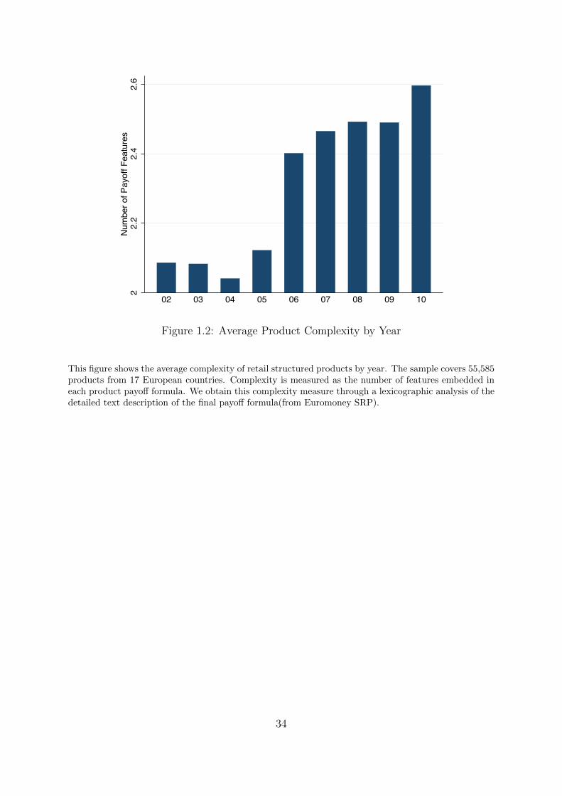
22.

22.

42.

6N

umbe

r of P

ayof

f Fea

ture

s

02 03 04 05 06 07 08 09 10

Figure 1.2: Average Product Complexity by Year

This figure shows the average complexity of retail structured products by year. The sample covers 55,585products from 17 European countries. Complexity is measured as the number of features embedded ineach product payo↵ formula. We obtain this complexity measure through a lexicographic analysis of thedetailed text description of the final payo↵ formula(from Euromoney SRP).

34

010

2030

40Fr

eque

ncy,

in %

2002-2004 2005-2007 2008-20101 2 3 4 5 1 2 3 4 5 1 2 3 4 5

Figure 1.3: Evolution of the Distribution of Product Complexity

This figure shows the evolution of the distribution of our complexity variable over three periods: 2002-2004, 2005-2007 and 2008-2010. The sample covers 55,585 products from 17 European countries. Com-plexity is measured as the number of features embedded in each product payo↵ formula. We obtain thiscomplexity measure through a lexicographic analysis of the text description of the final payo↵ formula(Source: Euromoney SRP).

35

10

20

30

40

50

60

Share

of P

roducts

in %

10

20

30

40

50

60

Implic

it V

ola

tilit

y

2002 2003 2004 2005 2006 2007 2008 2009 2010Offer Month

Implicit Volatility Ratio of Short Volatility Products

Figure 1.4: Ratio of Short Volatility Products and Implicit Volatility

This figure shows the share of short volatility products issued each month and the level of the implicitvolatility index over the 2002-2011 period. Short volatility products include products with one or severalfeatures that induce either a loss when the underlying index drops below a certain threshold or a cap onthe final payo↵ when the underlying index is above a certain threshold. These features are defined inthe Appendix. Implicit volatility is measured by the implied volatility index on European stock markets(VSTOXX, Source: Datastream).

36

5

10

15Pr

oduc

t Mar

k-up

s, in

%

-10

-5

00 200 400 600 800 1000 1200

Prod

uct M

ark

Product Complexity (Length of the Payoff Description, number of characters)

Figure 1.5: Description Length and Product Markups

This figure plots the markup of a product over its level of complexity for 101 products issued in July2009 and indexed to the Eurostoxx 50. Complexity is measured by the number of characters used intext description of the payo↵ formula of each product. We define markup as the di↵erence betweenthe o↵ering price and the fair market value we calculate through a local volatility model. We use theLongsta↵ and Schwartz OLS MonteCarlo pricing methodology in order to account for path dependence(Longsta↵ and Schwartz (2001)). Markups are expressed in % of notional, length in number of characters.Pay-o↵ descriptions are from Euromoney SRP.

37

2.1

2.2

2.3

2.4

2.5

2.6

Ave

rag

e N

b o

f F

ea

ture

s

-3 -2 -1 0 1 2Year to ETF Entry

Figure 1.6: ETF Entry and Financial Complexity

This figure plots the average product complexity as a function to the distance to ETF entry. Thecomplexity is defined as the number of payo↵ features as developed in section 3. The ETF entry ismeasured by the appearance of the search-term ”ETF” in Google Trend.

38

Table 1.1: Country-Level Summary Statistics

Country Total Issue Number of Number of % of % ofProducts Distributors Fin. Savings Mutual Funds

Since 2002 Since 2002 Since 2002 2010 2010(Billion Euros) (Percent) (Percent)

(1) (2) (3) (4) (5)

Italy 343 5,724 79 2.8 28Spain 204 4,734 60 2.8 37Germany 162 14,861 43 2.3 22France 158 1,801 73 2 12Belgium 135 4,021 46 8.5 69UK 110 6,135 141 1.1 8.3Netherlands 37 2,741 36 1.1 30Sweden 34 4,529 31 2 9Portugal 24 928 24 3.2 73Austria 20 3,275 42 3.3 28Denmark 17 563 31 .82 7.2Ireland 16 1,075 40 2.1 .91Norway 15 1,288 25 .28 1.6Finland 9 1,251 25 2.1 9.3Poland 8 1,518 45 1.5 19Czech Rep. 6 939 24 2.8 45Hungary 2 202 15 1.9 22

European Market 1,300 55,585 - 3 12.9

This table reports the aggregated volume of retail structured product issuance (column (1)), the totalnumber of products sold since inception (column (2)) and the number of distributors in each nationalmarkets (column (3)). Column (4) shows the penetration rate of retail structured products defined asthe share of household financial savings and column (5) compares the size of assets under management ofretail structured products to the one of the mutual fund industry. Retail structured products can take theform of a structured note, which is not included in the mutual fund industry. Figures in the table onlyinclude tranche products which are non-standardized structured products, with a limited o↵er period anda maturity date and which stand for 90% of the market in terms of volume. Flow products (e.g. bonus anddiscount certificates) and leverage products (e.g. warrants and turbos) are excluded (they stand for morethan 1 million issues since 2002 but only 10% of the market in terms of volume). Data is from EuromoneyStructured Retail Products.

39

Table 1.2: Product and Distributor Summary Statistics

Variable 2002-2004 2005-2007 2008-2010 Full Sample

(1) (2) (3) (4)

Underlying Type (in %)

Equity 82.1 77.5 70.5 76.6

Single Index 36.2 35.9 36.9 36.1

Single Share 2.9 9.5 7.5 8.1

Basket 42.9 32.1 26.1 32.3

Interest Rate 5.1 4.5 13.9 6.6

Commodity 0.6 5.5 4.0 4.5

FX Rate 1.8 3.1 4.6 3.2

Other 10.4 9.5 6.9 9.1

Distributor Type, Number (Market Share, in%)

Commercial Banks 102 (40.8) 132 (41.0 ) 133 (37.4 ) 172 (36.7)

Saving Banks 21 (8.4) 20 (6.2) 24 (6.7) 28 (6.0)

Private Banks 94 (37.6) 123 (38.2) 152 (42.7) 202 (43.1)

Insurance 23 (9.2) 30 (9.3) 31 (8.7) 40 (8.5)

Other 10 (4.0) 17 (5.3) 16 (4.5) 27 (5.8)

Total 250 324 357 471

Product Format (in %)

Non Collateralised Assets 61.0 83.9 88.4 81.7

Security 44.6 69.7 76.6 67.7

Deposit 16.5 14.2 11.8 14.0

Collateralised Assets 39.0 16.1 11.6 18.3

Life Insurance Product 6.9 6.3 4.6 6.0

Fund 31.8 9.6 7.0 12.1

Pension 0.3 0.2 0.1 0.2

Volume (in million Euros)

Mean 38.6 18.6 14.9 20.5

10th percentile 5.9 3.5 2.0 3.2

90th percentile 84.0 30.0 27.0 40.0

Product Design

Capital Guarantee (in %) 82.3 62.0 55.4 60.9

Average Maturity (in years) 5.0 4.3 4.0 4.2

This table reports summary statistics of characteristics of retail structured products in terms of underlyingasset, distributor type, format, volume and design. The sample covers 55,585 products from the 17 Europeancountries listed in Table 1, and data is from Euromoney SRP.

40

Table 1.3: Typology of Retail Structured Product Features

Families of Facultative Features

(1) (2) (3) (4) (5) (6) (7)

InitialSubsidy

Underly-ingSelection

ExposureModula-tion,Downside

ExposureModula-tion,Upside

PathDepen-dance

Exoticcondi-tion

EarlyRedemp-tion

# # # # # # #

Main Feature

1. Call ! Final Product:

2. Put! Each product includes one main feature

3. Spread! and 0 to 7 facultative features

4. Pure Income! with a maximum of 1 per family

5. Digital!6. Floater!

This table describes how a pay-o↵ formula is broken down into distinct features. Each family of facultativefeatures contains features that are mutually exclusive. A structured product possesses exactly one mainfeature, which defines the primary structure of the product. Details of each feature are provided in appendix.

41

Table 1.4: Measuring Complexity

Example 1: Example 2:Unigarant: Euro Stoxx 50 2007 Vivango Actions Mars 2017

DetailsYear 2002 2010Country Germany FranceProvider Volksbanken Rai↵eisenbanken La Banque Postale

Description This is a growth product linked to theperformance of the DJ Eurostoxx50.The product o↵ers [100% capital guar-antee at maturity ](1) along with a [pre-determined participation in the rise ofthe underlying ](1) over the investmentperiod

This is a growth product linked to abasket of 18 shares selected as beingthe largest companies by market cap-italization from within the eurostoxx50at the time the product was launched.Every year, the average performance of[the three best-performing shares ](2) inthe basket compared to their initial lev-els is recorded. These three shares [arethen removed ](2) from the basket. Atmaturity, the product o↵ers [a mini-mum capital return of 100%, plus 70%of the average of these performances ](1)

[recorded annually throughout the in-vestment period ](3).

[...](x): Text identifying Payo↵ x

Payo↵ Features Call Call - Himalaya - Asian Option

Complexity MeasuresNb Payo↵s 1 3Nb Scenarios 1 1Length 226 537

This table displays two real-life examples of product description, and shows how we convert these textdescriptions into quantitative measures of complexity.

42

Table 1.5: Increasing Complexity

Nb Payo↵s Nb Scenarios Length

(1) (2) (3) (4)

Specification 1

Year Trend 0.057*** 0.053*** 0.059*** 14.71***(0.015) (0.011) (0.013) (3.16)

Specification 2

2003 0.078 0.161 0.180 10.43(0.088) (0.097) (0.047) (9.50)

2004 0.049 0.103 0.172 29.58(0.089) (0.096) (0.039) (8.54)

2005 0.121 0.105 0.275 56.67(0.106) (0.114) (0.051) (11.17)

2006 0.271 0.294 0.371 87.33(0.100) (0.087) (0.064) (12.83)

2007 0.292 0.342 0.426 103.09(0.094) (0.086) (0.061) (12.41)

2008 0.337 0.380 0.366 100.36(0.088) (0.084) (0.060) (12.52)

2009 0.378 0.384 0.451 110.42(0.111) (0.083) (0.076) (17.22)

2010 0.453 0.434 0.613 129.34(0.106) (0.084) (0.072) (15.45)

Underlying FE Yes Yes Yes YesDistributor FE Yes Yes Yes YesProduct Format FE Yes Yes Yes YesCountry FE Yes Yes Yes YesVolume Weight No Yes No NoMaturity Yes Yes Yes Yes

Observations 54,716 52,478 54,716 54,716

This table displays the coe�cient of OLS regressions in which the dependent variables are our complexitymeasures, i.e. the number of pay-o↵s, the number of scenarios, and the length of the descriptive. Theexplanatory variables are respectively a year linear trend and year dummies in first and second specification.Number of payo↵s features is obtained through a lexicographic analysis of the detailed pay-o↵ descriptives.Number of scenarios is constructed by counting the number of conditions in the product descriptives. Lengthis the number of characters of the payo↵ descriptives. Standard errors are clustered at the distributor level.Data is from Euromoney SRP.

43

Table 1.6: Complexity Measures and Financial Sophistication

Nb Payo↵s Nb Scenarios Description Length(1) (2) (3)

Summary Statistics

Savings BankMean 2.7 2.7 533Standard Deviation 1.1 1.6 227Max 8 16 2,595

Private BankingMean 2.5 2.2 503.9Standard Deviation 1.1 1.5 213Max 7 9 2,102

Commercial BankMean 2.3 2.0 472.8Standard Deviation 1.1 1.4 206Max 7 11 2,203

OtherMean 2.5 2.2 503.9Standard Deviation 1.1 1.5 213Max 7 9 2,102

OLS Estimation

Savings Bank 0.168** 0.217** 46.840**(0.082) (0.103) (23.375)

Private Bank 0.126* -0.014 4.537(0.068) (0.085) (12.543)

Controls

Underlying FE Yes Yes YesProduct format FE Yes Yes YesYear FE Yes Yes YesVolume Yes Yes YesMaturity Yes Yes Yes

Observations 54,716 52,416 54,716

The upper half of the table displays summary statistics of our three measures of complexity by distributortype. The bottom half of the table displays OLS regressions in which the dependent variables are ourthree measures of complexity. The explanatory variables are dummy variables indicating the type of thedistributor. Number of payo↵ features is obtained through a lexicographic analysis of the detailed pay-o↵descriptive. Number of scenarios is constructed by counting the number of conditions in the product de-scriptive. Length is the number of characters of the payo↵ descriptive. Data is from Euromoney StructuredRetail Products.

44

Table 1.7: Product Complexity and Profitability

Product Yearly Markup, in %

Disclosed PDEFees Incl. Pricing

(1) (2) (3) (4) (5) (6)

# Payo↵s 0.33*** 0.30** 0.36*** 0.28* 0.36** 0.41**(0.11) (0.12) (0.11) (0.18) (0.15) (0.20)

Credit Risk Dummy -0.36 -0.14 -0.35 -0.43 -1.64*** -0.34(0.27) (0.54) (0.27) (0.31) (0.44) (0.43)

ControlsCountry FE Yes Yes Yes Yes Yes YesYear FE Yes Yes Yes Yes Yes YesDistributor FE - Yes - - - -Main Feature FE - - Yes Yes - -Facultative Feature FE (Main) - - - Yes - -

Observations 148 148 148 148 148 108R2 0.240 0.547 0.332 0.402 0.458 0.078

This table displays coe�cients of OLS regressions, in which the dependent variable is the yearly markup inpercent of product notional for all the products indexed to the Eurostoxx 50 sold in Europe in July 2009(101 products), as well as a random sample of 47 products indexed to the Eurostoxx in 2010. Markupsare computed as the di↵erence between the o↵ering price and the product calculated fair value, which weobtain by using Longsta↵ and Schwartz OLS MonteCarlo pricing methodology (Longsta↵ and Schwartz(2001)) with a local volatility di↵usion. Volatility surface data is from Eurex. The explanatory variableis the number of payo↵ features. Control variables include country fixed e↵ects, distributor fixed e↵ects,as well as main and facultative feature fixed e↵ect. Standard errors are clustered at the distributor grouplevel (30 clusters), and reported into brackets.

45

Table 1.8: Product Complexity and Ex-post Performance

Product Yearly Return, in %

All ESTX50 All ESTX50 All ESTX50(1) (2) (3) (4) (5) (6)

# Payo↵s -0.290* -0.273(0.175) (0.362)

# Scenarios -0.444** -0.207(0.212) (0.228)

Description -0.002** -0.003Length (0.001) (0.003)

ControlsCountry FE Yes - Yes - Yes -Distributor FE - Yes - Yes - YesUnderlying FE Yes - Yes - Yes -Year FE Yes Yes Yes Yes Yes YesCredit Risk Dummy Yes Yes Yes Yes Yes YesCapital Protection FE Yes Yes Yes Yes Yes Yes

Observations 7,467 968 7,467 968 7,467 968R2 0.415 0.209 0.417 0.211 0.417 0.216

This table displays coe�cients of OLS regressions, in which the dependent variable is the yearly rate ofreturn for growth products that have reached their term. Growth products only have one final pay-o↵.Columns (2), (4) and (6) restrict the sample on products indexed to the Eurostoxx 50. The explanatoryvariables are our complexity measures: number of pay-o↵ features (columns (1) and (2)), number of scenar-ios (columns (3) and (4)), and the length of the pay-o↵ description (columns (5) and (6)). Control variablesinclude country, year, distributor, underlying asset, and capital protection fixed e↵ects and a credit riskdummy for products that are non-collateralized. Standard errors are clustered at the distributor level, andreported into brackets. Performance data is from Euromoney SRP.

46

Table 1.9: The Impact of ETF Introduction on Complexity

Panel A Country Level

Nb Payo↵s Nb Payo↵s (> 1)(1) (2) (3) (4) (5)

ETF entry ⇥ Year � t 0.279*** 0.305*** 0.251***(0.087) (0.092) (0.087)

ETF entry ⇥ Year = t� 1 -0.045 0.012(0.107) (0.083)

ETF entry ⇥ Year = t 0.146 0.177(0.117) (0.115)

ETF entry ⇥ Year > t 0.331** 0.421***(0.166) (0.157)

ControlsCountry FE Yes Yes Yes Yes YesYear FE Yes Yes Yes Yes YesBanking Sector Profitability - Yes - - -

Observations 112 83 105 112 105R2 0.650 0.725 0.669 0.457 0.493

Panel B Distributor Level

Nb Payo↵s(1) (2) (3) (4) (5)

ETF entry ⇥ Year � t 0.108*** 0.095*** 0.032(0.018) (0.022) (0.036)

ETF entry ⇥ Year = t� 1 -0.010 -0.009(0.023) (0.044)

ETF entry ⇥ Year = t 0.078*** 0.008(0.028) (0.053)

ETF entry ⇥ Year > t 0.277*** 0.165**(0.039) (0.077)

ControlsCountry FE Yes Yes Yes Yes YesYear FE Yes Yes Yes Yes YesDistributor FE Yes Yes Yes Yes YesDistributor-Year FE - - - Yes YesIssued Volumes Yes Yes Yes Yes YesBanking Sector Profitability - Yes - - -

Observations 2,479 1,639 2,479 2,479 2,479R2 0.809 0.838 0.821 0.930 0.933

This table displays coe�cient of OLS regressions on unbalanced panel data at the distributor-country levelover the period 2002-2010. All countries are included except Norway over the 2008-2010 period due to a banon structured products, and Hungary and Poland due to insu�cient volumes. The dependent variable isthe average complexity of products for a given country in a given year (Panel A), and for a given distributorin a given country and for a given year (Panel B). The di↵erence-in-di↵erences methodology is based onthe staggered entries of ETF across European countries. ETF is a dummy which is equal to one onceETFs have been introduced in a given country, as measured by the appearance of the search-term ”ETF”in Google Trend. Standard errors are clustered at the distributor level, and reported into brackets.

Table 1.10: Competition and Complexity: Number of Competitors

Panel A Country Level Distributor Level

# Payo↵s # Types # Payo↵s(1) (2) (3) (4) (5) (6)

# Competitors 0.012** 0.019** 2.338*** 4.139*** 0.009* 0.016***

(0.005) (0.009) (0.818) (0.789) (0.005) (0.006)

Controls

Country FE Yes Yes Yes Yes Yes YesYear FE Yes Yes Yes Yes Yes YesDistributor FE - - - - Yes YesBanking Sector Profitability - Yes - Yes - Yes

Observations 132 101 132 101 2,507 1,682R2 0.553 0.578 0.812 0.854 0.444 0.462

Panel B Country Level Distributor Level

# Payo↵s # Types # Payo↵s(Change) (Change) (Change)

(1) (2) (3) (4) (5) (6)

� # Competitors -0.001 -0.008 1.499*** 2.072*** 0.010** 0.010*

(0.004) (0.007) (0.558) (0.525) (0.005) (0.006)

Controls

Year FE Yes Yes Yes Yes Yes YesBanking Sector Profitability - Yes - Yes - Yes

Observations 117 88 117 88 1,822 1,183R2 0.001 0.017 0.204 0.382 0.005 0.009

This table displays coe�cient of OLS regressions on unbalanced panel data at the country and distributorlevel over the period 2002-2010. All countries are included except Norway over the 2008-2010 period due toa ban on structured products, and Hungary and Poland due to low representativeness. Volume sold sinceinception has been lower than 10 million euros in these countries standing for less than 2% of financialsavings. In panel A, the dependent variable is the average complexity of products, measured at the countryx year level for columns 1 and 2, and at the distributor level for column 4 and 5. The dependent variableof column 3 is the number of product varieties o↵ered in a country a given year. The explanatory variablefor all columns is the number of competitors in the retail market for structured products at the country xyear level. In panel B, the dependent variables are the yearly absolute change of the previously describedvariables. Banking sector profitability represents the aggregate amount of profit by bank in a given countryand a given year. Standard errors are robust to heteroskedasticity in columns 1 to 3, and clustered at thedistributor level in columns 4 and 5, and reported into brackets.

48

Chapter 2

Political Incentives and Financial

Innovation

The Strategic Use of Toxic Loans by Local Govern-

ments

Joint work with Christophe Perignon (HEC Paris)

Everything is possible, from angels to demons to economists and politicians. [Paulo

Coelho]

50

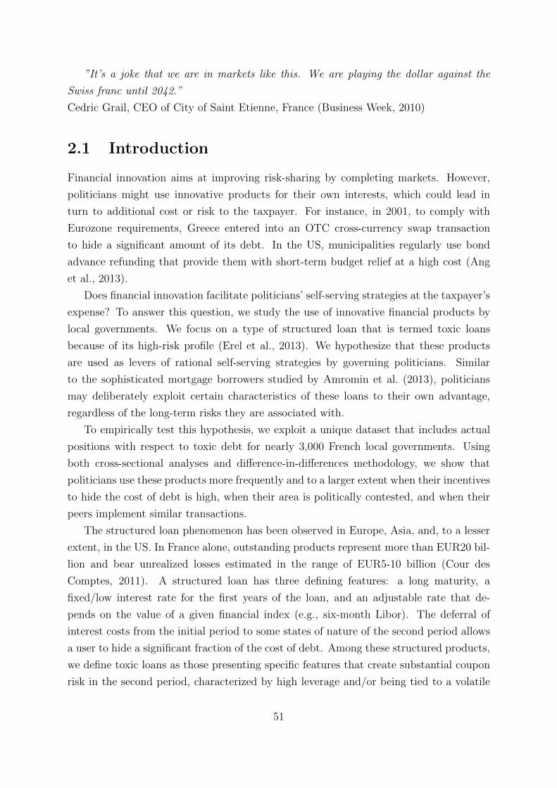
”It’s a joke that we are in markets like this. We are playing the dollar against the

Swiss franc until 2042.”

Cedric Grail, CEO of City of Saint Etienne, France (Business Week, 2010)

2.1 Introduction

Financial innovation aims at improving risk-sharing by completing markets. However,

politicians might use innovative products for their own interests, which could lead in

turn to additional cost or risk to the taxpayer. For instance, in 2001, to comply with

Eurozone requirements, Greece entered into an OTC cross-currency swap transaction

to hide a significant amount of its debt. In the US, municipalities regularly use bond

advance refunding that provide them with short-term budget relief at a high cost (Ang

et al., 2013).

Does financial innovation facilitate politicians’ self-serving strategies at the taxpayer’s

expense? To answer this question, we study the use of innovative financial products by

local governments. We focus on a type of structured loan that is termed toxic loans

because of its high-risk profile (Erel et al., 2013). We hypothesize that these products

are used as levers of rational self-serving strategies by governing politicians. Similar

to the sophisticated mortgage borrowers studied by Amromin et al. (2013), politicians

may deliberately exploit certain characteristics of these loans to their own advantage,

regardless of the long-term risks they are associated with.

To empirically test this hypothesis, we exploit a unique dataset that includes actual

positions with respect to toxic debt for nearly 3,000 French local governments. Using

both cross-sectional analyses and di↵erence-in-di↵erences methodology, we show that

politicians use these products more frequently and to a larger extent when their incentives

to hide the cost of debt is high, when their area is politically contested, and when their

peers implement similar transactions.

The structured loan phenomenon has been observed in Europe, Asia, and, to a lesser

extent, in the US. In France alone, outstanding products represent more than EUR20 bil-

lion and bear unrealized losses estimated in the range of EUR5-10 billion (Cour des

Comptes, 2011). A structured loan has three defining features: a long maturity, a

fixed/low interest rate for the first years of the loan, and an adjustable rate that de-

pends on the value of a given financial index (e.g., six-month Libor). The deferral of

interest costs from the initial period to some states of nature of the second period allows

a user to hide a significant fraction of the cost of debt. Among these structured products,

we define toxic loans as those presenting specific features that create substantial coupon

risk in the second period, characterized by high leverage and/or being tied to a volatile

51

underlying index (e.g., foreign exchange rate). Such loans typically o↵er low initial rates.

During the recent financial crisis, as volatility spiked, the interest costs of toxic loan

users increased to historically high levels and may even remain high for the remainder

of their lifetimes. An interesting example is the City of Saint-Etienne, the 14th largest

French city, which is currently suing its banks for pushing financial products that were

alleged to be excessively risky. In 2010, the annual interest rate charged to one of its

major loans increased from 4% to 24% as it was indexed on the British pound/Swiss franc

exchange rate (Business Week, 2010). The total unrealized losses on Saint-Etienne toxic

products reached EUR120 million in 2009, nearly doubling the city’s nominal debt level

of EUR125 million (Cour des Comptes, 2011). To obtain a sense of the geographic spread

of structured debt among French local governments, Figure 2.1 displays an activity map

for the second quarters of four consecutive years (2004-2007). The onset of toxic loans

occurred around 2000; the market, which was largely developed by 2005, peaked in 2007.

INSERT FIGURE 2.1

Although both global and severe, the toxic loan phenomenon remains underinvesti-

gated.1 This lack of research primarily results from a lack of comprehensive data. We rely

on two proprietary datasets that adequately complement one another. The first dataset

contains the entire debt portfolio for a sample of large French local governments as of the

end of 2007. For each debt instrument, we access information pertaining to the notional

amount, maturity, coupon rate, type of product, underlying financial index, and lender

identity. The second dataset includes all of the structured transactions made by Dexia,

the leading bank on the French market for local government loans, between 2000 and

2009. This dataset provides loan-level information, including the mark to market and

transaction date. This latter variable is critical for our identification strategy. Unlike the

financial statements of local governments that do not distinguish structured loans from

standard borrowing, these datasets provide detailed information on the types of loans

that are used by each local government. In turn, these data allow us to address whether

agency conflicts a↵ect the financial decisions of politicians.

We provide empirical evidence of the self-serving use of toxic loans by politicians. We

begin by showing that structured loans account for more than 20% of all outstanding debt.

More than 72% of the local governments in our sample use structured loans. Among these

structured loans, 40% are toxic. A cross-section of our data illustrates how politicians

in financially distressed local governments are significantly more likely to turn to this

type of loan, evidencing their higher incentive to hide the cost of debt. Indeed, local

governments in the top quartile of indebtedness are more than twice as likely to have

1Capriglione (2014) studies the use of derivatives by Italian Local Governments.

52

toxic loans compared with those in the bottom quartile. We also find that incumbent

politicians running in politically contested areas are more inclined to use toxic loans,

which is consistent with the greater incentives to benefit from immediate savings to aid

them in being re-elected.

We then exploit the time dimension of our data. We identify a treatment group that

confronts elections during the sample period, as opposed to a control group that does not

appoint management through elections (e.g., airports, harbors, and hospitals). Using a

di↵erence-in-di↵erences methodology on these two subsamples, we find that the election

timing plays a significant role: for the with-election group, transactions are more frequent

shortly before elections than after them. Toxic loan usage also exhibits a herding pattern;

politicians are more likely to enter into toxic loans if some of their neighbors have done

so recently. This herding behavior reduces reputation concerns, while increasing the

likelihood of a collective bail-out. Finally, we find that right-wing political parties are

more likely to engage in structured loans to cater to the fiscal expectations of their voters

while hiding the real costs of their strategy in some states of nature. Although measuring

the exact role and extent of financial sophistication (Lusardi and Tufano, 2009b) is beyond

the scope of this study, we control for this factor in our analysis to ensure that it is not

driving our results. We also empirically eliminate the possibility of hedging as a motive

for these transactions.

Our paper relates to several streams of literature. First, our work complements studies

of the political agency problems (Besley and Case, 1995), political incentives (Rajan,

2010), their influence on financial decisions (Butler et al., 2009), and more generally on

the political economy of finance: Dinc (2005) shows that government banks lend more in

election years, and (Bertrand et al., 2007) document that politicians avoid layo↵s prior

to French elections. The main contribution of the paper is to show how politicians use

innovative financial products for their own interests, and (Behn et al., 2014) investigate

the e↵ects of political determinants on bank bailouts.

Because toxic loans allow local governments to hide a significant fraction of the cost

of debt, our work directly relates to the o↵-balance sheet borrowing of local governments

(Novy Marx and Rauh, 2011). This study also adds to the abundant literature on peer

e↵ects and herding behavior in financial markets (Hong et al., 2005). Unlike previous

studies on herding, we focus on the economic decisions of politicians. Finally, our paper

addresses financial innovation and the associated risks (Rajan (2006), Gennaioli et al.

(2012)). The paper proceeds as follows. In Section 2, we present the main types of

structured loans and identify the toxic types. We describe our datasets in Section 3 and

present our empirical analysis in Section 4. We conclude our study in Section 5.

53

2.2 The Toxic Loan Market

This section explains the specifications and functioning of structured debt, defines toxic

loans, and provides a real-life example of a toxic loan. These characteristics were identified

from product term sheets and abundant discussions with professionals from both buy and

sell sides.

2.2.1 Common Characteristics of Structured Loans

Structured loans typically o↵er an initial period with a guaranteed low interest rate and

a second period during which the interest rate may increase according to an explicit

pre-specified formula. The loan structuring relies on an implicit sale of options by the

borrowing local government. The options premium is initially subtracted from the interest

cost. The risk of a structured product increases with its maturity, the volatility of the

underlying financial index, the leverage in the coupon formula, and the cap level. We

provide a real-life example at the end of this section and detail how toxic loans translate

into hiding the actual cost of debt.

Under most government accounting standards, derivatives (either stand-alone swaps

or those embedded within a structured loan) are not accounted for at fair value. In many

countries, accounting standards do not even require the structured transactions to be

disclosed. Only the interests that are actually paid must appear in financial statements;

thus, a derivative, regardless of the evolution of its fair value and future cash flows, will

generate accounting revenues as long as the flows that it creates in a given accounting

year favor the local government. By construction, this situation always occurs during the

initial low-interest period of three to five years, regardless of the market evolution during

that time. Losses can appear in financial statements only when the guaranteed period is

over.

Long-maturity debt is a prerequisite for structuring products with initial periods

of low interest rates. Local governments are among the issuers that have the longest

horizon. Furthermore, only local governments have the credit quality that is necessary

for banks to accept such long credit exposure, which cannot be perfectly hedged. In

discussions with practitioners, we learned that these transactions are also significantly

more profitable than vanilla loans (approximately 5% of mark-up for toxic loans vs. less

than 1% for vanilla loans). Counterparty risk is likely to be underestimated because

of the widespread view that the state is implicitly guaranteeing local governments. As

opposed to corporate clients, no collateral is required. Such requirements would jeopardize

structured transactions, as the negative fair value of a derivative position would lead to

immediate margin calls.

54

Structured products are easily transposable from one country to another. The legal

documentation is limited to a three- or four-page contract. Structuring mechanics rely

on worldwide known indices, such as the US Libor or EURUSD exchange rate. As

global players, financial institutions simultaneously market the same products in di↵erent

countries. Even if their di↵usion is global, market penetration is higher in Europe than in

the US, partly because cities and regional governments in Europe receive their financing

primarily from banks whereas those in the US primarily raise funds by issuing bonds.

Therefore, local governments in Europe may be more easily persuaded to use structured

products. Another critical di↵erence between Europe and the US concerns the level of

complexity of the products. Indeed, local governments in Europe use much more complex

products. Complexity often increases each time a product class must be restructured.

2.2.2 Which Structured Loans Are Toxic?

While some structured loans appear as toxic in the sense that local government are

currently paying double-digit coupon rates, classifying their risk objectively ex ante is not

trivial. We rely on the classification established by the French Government following the

first legal actions: the Gissler Chart. Indeed, although they rely on the same mechanism

(an implicit sale of options, the premium of which is subtracted from the initial coupon

rate), structured loans exhibit diverse risk profiles, which correspond to di↵erent level of

short term budget relief: the riskier a product, the higher the initial savings. The Gissler

Chart classifies structured loans along two dimensions: the underlying asset, and the pay-

o↵ structure. This scale ranges from Eurozone interest rate (minimum risk), to foreign

exchange (maximum risk), and is based on the volatility of these underlying. For more

details regarding the di↵erent types of structured loans, and the Gissler Classification,

see the appendix.

We classify a structured product as toxic if it ranks higher than 3 on the Gissler Chart

underlying risk table. Given this definition, loans that are indexed on the interest rate

curve slope, foreign interest rates or on a foreign exchange rate are classified as toxic.

Products that are linked to domestic interest rates or inflation are not considered toxic.

We also use the full granularity of this risk classification.

This classification is ex ante based on the characteristics of a product at inception and

is independent from the market conditions that prevail during the life of the product. A

toxic product may have o↵ered a low coupon level to its user ex post; nevertheless, the

borrower entered into a high-risk transaction that would have created massive losses had

the market situation been reversed. Furthermore, toxic products often exhibit swings

in their mark to market. Structured products that are not classified as toxic still bear

more risk than vanilla financing. The subsidy that such products o↵er in the favorable

55

state of the world is financed by a higher coupon than in the unfavorable state. The

nonlinear payo↵s of such loans are also challenging to manage in practice, as they can

create moderate but sudden increases in the cost of debt. Importantly,

2.2.3 Example of a Toxic Loan

Below, we present an actual toxic loan subscribed by the Rhone, the French county that

comprises the city of Lyon. We observe an eight-year initial period with a low guaranteed

coupon of 1.75%, which is significantly lower than the interest rate on an equivalent vanilla

loan (slightly higher than Euribor or 4.50%). This initial fixed low rate is followed by

a 12-month Euribor floating rate, coupled with uncapped exposure to CHF appreciation

against EUR for the remaining 17 years. At today’s levels (as of May 2014), the interest

rate on this loan is more than 16%. Similar products with higher leverage or strikes have

led some local governments to pay more than a 50% interest rate per year.

Amount : EUR 80 million

Trade Y ear : 2006

Loan Maturity : 2031

Y ear 2006� 2013 : Coupon(t) = 1.75%

Y ear 2014� 2031 : Coupon(t) = EURIBOR 12M(t)� 0.80%⇥Max(1.40/EURCHF (t)� 1, 0%)

2.2.4 Local Government Rationale

Toxic loans allow local governments to hide a significant fraction of the cost of their debt,

and to provide with a secure budget relief for the period where the coupon is guaranteed.

By deferring the payment of most of the interest of this period to a later date and only

in certain states of nature, a local government cosmetically decreases its current cost

of debt when entering into a toxic loan. Returning to the example in Section 2.3, the

product provides a 2.75% annual subsidy, which is the di↵erence between the rates on

an equivalent vanilla loan and those on a toxic loan. If the entire debt of the local

government consists in this type of financing, the cost of debt appear less than half than

what it should be. This hidden cost of debt is repaid in the future in certain states of

nature, namely, when the options embedded in the derivative component of the loan end

up in the money. The details of structured loans do not appear in public filings; only

their current interest rates appear. This lack of disclosure makes toxic loans di�cult to

detect for voters and therefore permits local governments to cosmetically reduce their

cost of debt.

56

2.2.5 Post-crisis developments

The spike in market volatility triggered by the financial crisis drove the derivative mark-

to-markets up, and often led the options to get in the money. Starting in 2010, local

governments have been unwilling to pay two digit interest rates, and have been suing

banks for mis-advice and questioned the validity of the transactions. They try to obtain

the cancellation of the toxic loans, or to negotiate an exit at better terms. Court out-

comes have been mixed, but led to the cancellation of the structured loans that had not

stipulated an actuarial rate when implemented.

A nationwide solution has however been implemented in 2014, in the form of a 50%

participation of the central government in the unwinding costs. This spending is financed

by a new tax on banks, which exact amount has still to be fixed. This development

represents a partial bail-out, and exhibit a trade-o↵ between having only local taxpayers

pay for the toxic loans, or sharing it over the entire French population. An additional

issue facing the central government is that the main player in the market, Dexia, has

been nationalized during the crisis. Therefore forfeiting all the mark-to-markets would

be extremely costly for the French Government.

2.3 Data

Our unique datasets allow us to provide new insight into the e↵ect of political incentives

on the borrowing choices of local governments. Indeed, these data enable us to analyze

risky strategies that are hidden from the public view. In most countries, the financial

statements of local governments do not present the precise breakdown of debt by instru-

ment. In particular, structured loans and swaps are not distinguished from vanilla loans.

Whereas aggregate debt analysis can be conducted using public information only, our

analysis of toxic loans requires that we know the exact composition of the debt portfolio

of each local government. This requirement can be met using two proprietary datasets.

The first dataset contains the entire debt portfolio for a sample of large French local

governments (Dataset A) as of December 31, 2007. The second set includes all of the

outstanding structured transactions of the leading bank on the market (Dataset B) as of

December 31, 2009.

2.3.1 Local Government-Level Data from a Leading Consulting

Firm (Dataset A)

A leading European financial consulting firm for local governments provided us with a

detailed proprietary dataset for a sample of 293 French local governments. As shown in

57

Table 2.1, our dataset includes nearly all French regions (25) and French counties (96)

as well as a number of intercity associations (76) and the largest cities (96). Collectively,

these local governments have a total debt of EUR52 billion. Although our sample covers

only a fraction of the French local governments, the overall debt coverage is extensive,

as it includes the largest entities. Indeed, the sample aggregate debt represents 38.2%

of the total debt of all French local governments and more than 52% of their structured

debt (Fitch Ratings, 2008).

INSERT TABLE 2.1

We observe that virtually all local governments (95.6%) have some type of debt, and

this fraction remains high for all types of local governments. However, the standard

deviations and min-max ranges indicate that there are some large di↵erences in the levels

of indebtedness across local governments. The lower panel of Table 2.1 indicates that the

maturity of the debt is on the long side (in the range of 12-15 years).

INSERT TABLE 2.2

Table 2.2 presents the breakdown by type of debt. Funding is achieved through the

following channels: vanilla bank loans, bonds, revolving facilities, and structured debt.

Overall, we find vast di↵erences across local governments in terms of debt instruments.

Some municipalities borrow through a single source (e.g., fixed rate loans, floating rate

loans, structured debt, or revolving facilities), whereas others follow a more diversified

financing strategy. Bank loans are by far the main source of financing for local gov-

ernments (constituting 62.9% of outstanding debt and being used by more than 90% of

local governments), with an approximately 50/50 breakdown between fixed and floating

rates. Bonds account for a surprisingly low percentage of total debt: 3.3% of outstanding

debt. Bonds are used by only 7.5% of local governments, likely because of the relatively

higher cost for bonds and the numerous constraints that issuers encounter (rating re-

quirements, the legal framework, and constraints on maturity) and that are not o↵set by

tax breaks, as is the case in the US. It is interesting to compare the debt composition of

local governments with that of the French Central Government, which comprises almost

only bonds and bills. Finally, structured debt represents a significant share of the total

debt of local governments, accounting for 20.1% of all outstanding debt and being used

by more than 72% of the local governments in our sample. These ratios are particularly

high for counties and cities. The fraction of structured debt varies extensively across local

governments. Interestingly, we observe that 100% of the debt of some local governments

is in structured products.

58

We now examine the specific composition of the structured debt of local governments.

It is important to di↵erentiate between the di↵erent types of structured products because

they convey di↵erent levels of risk and because some structured products should not

be considered toxic. A detailed breakdown of structured debt by type of structured

product can be found in the appendix. The most popular products are those linked to

domestic interest rates, which account for nearly half of the outstanding structured debt

(47.7%). Other underlying indices (sorted by decreasing popularity) include the interest

rate curve slope (26.8%), foreign exchange (14.8%), inflation (3.4%), and foreign interest

rates (2.4%). Despite this overall range of products, there is significant heterogeneity

among local governments. Some of these governments are massively exposed to toxic

loans, with up to 70.5% of their total debt being exposed to the interest rate curve slope

or 66.7% of the total debt to foreign exchange rate variations.

2.3.2 Bank-Level Data on Structured Transactions from Dexia

(Dataset B)

Our second dataset is 10 times larger than the first set and contains detailed informa-

tion on the structured products themselves. This internal risk management data were

made public by the French newspaper Liberation on its website and, to the best of our

knowledge, have not yet been used in academia. The dataset contains information on

structured transactions from only one bank (i.e., Dexia), but this bank has a 70% mar-

ket share for public sector-structured loans (French National Assembly, 2011) and an

extremely diverse customer base. Moreover, the data covers structured transactions over

the period 2000-2009, which allows time-series analysis.

This dataset contains 2,741 di↵erent public sector entities: 16 regions (vs. 25 in

Dataset A); 66 counties (vs. 96); 539 intercities (vs. 76); 1,588 municipalities (vs. 96);

288 hospitals (vs. zero); 115 social housing entities (vs. zero); and 129 other borrowers, in-

cluding airports, harbors, chambers of commerce, healthcare cooperatives, public-private

joint ventures, schools, research institutes, nursing homes, fair organizers, and charities.

The local governments in our sample vary significantly in terms of size; for instance, 37

cities have fewer than 1,000 inhabitants, and 29 cities have more than 100,000 inhabitants.

INSERT TABLE 2.3

Table 2.3 provides summary statistics on the number of trades, notional amounts

of structured products, associated mark to market, and foreign exchange-linked toxic

products. The average number of structured transactions is approximately two, but 163

entities have more than five structured loans in their debt portfolio. On average, counties,

59

regions, and social housing entities engage in more structured loans than other entities,

likely because of the size of their total debt, as they are the largest entities. The notional

amounts of structured products exhibit the same pattern but with greater dispersion

across various types of borrowers.

Some mark to market figures are surprisingly high: 72 entities have more than EUR10

million of mark to market, with additional products potentially booked in other banks.

Therefore, it would be extremely costly for these entities to convert their structured

debt into vanilla debt. Counties are again the most strongly a↵ected local governments

according to this indicator, followed by regions. The mark to market scaled by notional

amounts illustrate products’ relative risk ex post and expected future losses to bear on

top of principal repayment. Although these losses should be absorbable on average, as

they represent approximately 10% of the borrowed amount through structured products,

a fat tail of aggressive products with mark to market greater than 30% of the underlying

notional amount increases the risk of default for some entities.

This tail risk largely results from foreign exchange products. Their frequency appears

to be consistent with our observation from the previous dataset, in which 20% of the local

governments using structured debt had foreign exchange products in their portfolios.

These figures indicate that the level of contamination is severe for some entities, as

their mark to market values sometimes reach record levels of 80% of the underlying

loan notional amount. The data also include information on trade initiation dates. The

aggregated numbers of transactions per quarter are plotted in Figure 2.2. We observe

the rapid expansion of the market followed by a sharp contraction after 2007. The latter

was exacerbated by media coverage of distressed local governments and by banks’ own

di�culties in 2008Q4.

INSERT FIGURE 2.2

2.4 Empirical Analysis

In this section, we study the role of political incentives in fostering the use of structured

and toxic loans among local governments.

2.4.1 Incentives to Hide the Cost of Debt

Given their accounting treatment, structured products can be considered hiding a sig-

nificant fraction of the cost of debt, which will be repaid only in some specific states of

nature. Politicians have an incentive to hide the actual cost of debt and to spend money

today while shifting the tax burden onto future generations (Novy Marx and Rauh, 2011).

60

We hypothesize that the incentive to hide a fraction of the cost of debt will be greater

for highly indebted local governments, as monitoring by voters and other stakeholders is

likely to be closer.

INSERT TABLE 2.4

Panel A in Table 2.4 provides an initial overview of the popularity of toxic loan usage

for the top and bottom indebtedness quartiles of the local governments in Dataset A. The

panel shows unconditional statistics that suggest that highly indebted local governments

use structured and toxic loans more frequently and to a greater extent.

We extend the analysis in Table 2.5 and run several probit regressions on the use

of structured and toxic loans by local governments based on Dataset A. In columns 1

and 2 (3 and 4), the explained variable is an indicator variable that is equal to one if

the local government has some structured (toxic) products in its debt portfolio and zero

otherwise. Columns 5 and 6 present the coe�cients from an ordered probit regression in

which the dependent variable is equal to the sum of the two previous dummies; namely,

the dependent variable takes a value of two if toxic loans are used, one if structured but

not toxic loans are used, and zero otherwise. For each specification, we assess the robust-

ness of our conclusions using a set of extra control variables, including the debt average

maturity, population, banking relationships (indicator variables for lending relationships

with Dexia, Credit Agricole, Societe Generale, and others), and territory characteristics

(unemployment rate, share of agriculture, and industry in the active population). Fur-

thermore, we control for several other economic variables and for fixed e↵ects by local

government types (regions, counties, intercities, and cities) in each regression and cluster

standard errors by local government types.

INSERT TABLE 2.5

The results from Table 2.5 are consistent with the existence of greater incentives to

hide the actual cost of debt for local governments that are swamped with debt. Such

governments tend to use structured and toxic loans more frequently. Indeed the esti-

mated coe�cient on the debt/population is positive and statistically significant in all

specifications. Because the level of debt will be more closely monitored in these local

governments, they have stronger incentives to enter into such transactions. In a further

robustness check (not presented), we also include the operating income per inhabitant

and central government subsidy per inhabitant. Because regression coe�cients are not

statistically significant, we conclude that the debt burden dominates the e↵ects of rev-

enues or dependence on the central government. Another possible explanation for these

61

empirical results would be that indebted local governments turn to toxic loans as last-

resort financing when other means of financing are unavailable to them. However, our

data are inconsistent with this alternative hypothesis, as some highly indebted local gov-

ernments have no structured debt at all (thus, even these local governments can access

standard financing).

We also report a negative relationship between the use of structured products and

investments (measured by equipment expenditure per inhabitant). If we consider high

investment expenditure, as opposed to operating expenditure, to be a signal of sound

management, then it is reasonable to believe that well-managed local governments that

are concerned about the future are more reluctant to take unnecessary risks in the financial

markets. We believe that this negative coe�cient is not due to reverse causality. In

2007, most products were in their guaranteed coupon period; thus, it is unlikely that

local governments had to decrease their investments because of ballooning interest rates.

However, the absence of satisfying instruments for the use of these products prevents us

from using investments as a left-hand-side variable and being able to neatly identify the

real e↵ects of toxic loans. Oversta�ng, which signals short-term spending and is measured

through wages over operating costs, also shows a significant positive correlation with the

use of toxic loans.

Debt average maturity provides us with another important control, as toxic loans re-

quire long-maturity debt (recall that these loans rely on an implicit sale of options). The

type of banking relationship is also a critical driving factor for toxic loan usage. The pres-

ence of banks having a broad structured loan o↵ering in their financing pool significantly

increases the likelihood of a local government eventually using these products. The e↵ect

is greater for banks that specialize in loans to local governments, such as Dexia or Depfa,

than for universal banks.

To complement our analysis, in columns 7 and 8 of Table 2.5, we conduct additional

regressions to measure the extent to which the level of indebtedness influences borrowing

choices. We analyze the structured debt/total debt ratio, the toxic loans/total debt

ratio, and the foreign exchange loans/total debt ratio using OLS, thereby capturing the

extent to which these products have been used. We control for the exact same variables

as in Table 5. These additional regressions confirm our previous results regarding the

importance of the level of indebtedness. Thus, a per capita debt increase of EUR1,000

leads to an increase of more than 12.8% of the share of structured loans in the total debt

and 4.2% of the share of toxic loans. Table 6 also underlines the role of debt maturity,

especially for foreign exchange-linked toxic loans that exploit the long end of the FX

forward curves. Longer maturities also allow higher subsidies in a manner that is more

than proportional and thus magnify the temptation to hide the cost of debt.

62

2.4.2 Political Cycle

Toxic loans represent a way of hiding the real cost of debt. We hypothesize that the po-

litical cycle interacts with incentives to hide the cost of debt, thus creating cross-sectional

and time-series variations according to each local government’s political situation. When

their re-elections are likely to be contested or when the next election draws closer, in-

cumbent politicians may desperately seek immediate savings for a limited time, possibly

corresponding to their political mandate period. One means of achieving this short-term

financial release without raising the suspicion of voters is the use of structured financial

instruments. Toxic loans allow budget window dressing as a result of their initial low-

coupon guaranteed period, as mentioned previously. This hidden characteristic and the

accompanying short-term financial release may cause structured loans to be used more

frequently in politically contested areas, whereas strongholds should exhibit lower usage.

The timing of these transactions should also depend on the date of the next election in

a local government; incumbent politicians have an incentive to implement transactions

before the election to benefit from the immediate savings that they provide.

Politically contested areas

For a subsample of local governments in Dataset B for which past elections results are

available, we proxy political stability by the number of years for which the party of the

incumbent mayor (or its equivalent) has been in power. Toxic loans may catalyze agency

problems, as they allow politicians to implement hidden self-serving strategies. The data

appear to be consistent with this hypothesis. Indeed, Panel B in Table 4 illustrates

how politically contested local governments make more important use of structured loans

compared with political strongholds. We also conduct OLS regressions on three di↵erent

measures of the usage intensity of structured loans: (1) structured debt/total debt ratio,

(2) mark to market/total debt ratio, and (3) toxic debt/total debt ratio. The results are

presented in Table 2.6.

INSERT TABLE 2.6

The results in Table 2.6 provide further favorable evidence for a positive e↵ect of

political uncertainty on the use of toxic loans: strongholds are less inclined to enter into

these transactions. All of the estimated coe�cients on the number of years in power are

indeed significantly negative. This finding indicates the increased incentives for politi-

cians with challenging re-elections to enter into risky transactions, which can be either

a form of risk-shifting strategy or a poison pill for the next government because losses

require several years to materialize. It has been shown that political uncertainty reduces

firm investment (Julio and Yook, 2012), and we complement this stream of literature by

63

demonstrating the influence of this uncertainty on the economic decisions of politicians.

We control for political a�liations and the size of local authorities. The latter proxies

for financial sophistication, as larger local governments devote more sta↵ and resources

(e.g., consulting and software) to the management of their debt and thus have greater

expertise in this area.

Finally, our results indicate that small local governments use more structured prod-

ucts than large governments do. All three measures of the relative use of structured and

toxic loans are significantly negatively correlated with the log of the population. This

finding suggests that banks have more successfully marketed these products to clients

that are less likely to possess the su�cient financial knowledge to fully understand and

adequately monitor them. Small local governments appear to use structured loans in

larger quantities and to be more inclined to enter into the riskiest transactions; this

finding is consistent with overindebtedness patterns in households with low debt literacy

(Lusardi and Tufano, 2009b).

E↵ect of election timing

We use a di↵erence-in-di↵erences approach to test whether local governments engage

more frequently in structured debt prior to an election. We compare a treatment group

that includes counties, municipalities, and intercities that hold elections at the end of

2008Q1, with a control group consisting of public entities with no elections (e.g., hospitals,

social housing entities, and airports). The management teams of the entities from the

treatment group are chosen simultaneously following the same election cycle. Those

from the control group have management renewals according to individual and random

timing. The control group also includes political entities that have electoral cycles but no

election during that particular year (regions). We implement a di↵erence-in-di↵erences

methodology by comparing the di↵erence of the probability of implementing a trade

before and after the election between the two groups. The purpose of this approach is

to be able to precisely identify the influence of election timing on structured transaction

implementation. Using panel conditional logit regressions, we examine the likelihood of

implementing a structured transaction in a given quarter before and after the election

(for periods of 12 and 18 months before and after the election) by controlling for quarter

fixed e↵ects. The model specification is as follows:

Pr(Transaction)i,t

= Qt

+ ↵i

+ � ⇥ I{Treatment Group = 1 \ Pre Treatment = 1} + "i,t

where the dependent variable is the probability that local government i conducts a

transaction in quarter t, Qt

are the time fixed e↵ects for each quarter, ↵i

are individual

64

fixed e↵ects, and the I{Treatment Group = 1 \ Pre Treatment = 1} variable is an interaction term

between a dummy variable that is equal to one if local government i is in the treatment

group and a dummy variable that is equal to one if quarter t is before the election. The

results are shown in Table 2.7.

INSERT TABLE 2.7

When comparing to the control group with no elections, we observe that the local

governments in the treatment group are significantly more likely to implement structured

and toxic transactions in the period preceding the election than in the period following

it. The results are robust to the time window under consideration. We also conduct a

placebo analysis in which we randomly select a sample of the same size as our initial

treatment group and use it for the interaction term. The coe�cients obtained are smaller

in magnitude and statistically insignificant, which is consistent with our results being

driven by the election cycle.

2.4.3 Herding

Local government members and civil servants belong to strong local and political net-

works that facilitate word-of-mouth di↵usion. This channel of communication is critical

for triggering herding, as structured transactions typically remain private. Therefore,

peer e↵ects should play an important role in terms of both ignoring personal beliefs and

managing one’s reputation (Scharfstein and Stein, 1990) to create a cascade e↵ect. Fol-

lowing the crowd can indeed be a rational strategy. First, when structured products

perform well, structured loan users benefit from a low interest rate on their debt. Sec-

ond, when structured products perform poorly, all structured loan users confront the

same turmoil, and a collective solution must be found. This “risk taking from the herd”

also relates to models of collective moral hazard, as it increases the likelihood of being

bailed out if risk materializes (Farhi and Tirole, 2012). Therefore, the propensity of a

given local government to use structured loans increases with the number of contaminated

local governments in the same geographical zone.

To identify this behavior, we again exploit the time dimension of Dataset B. Although

the majority of the variables studied in the previous section exhibit low time variation,

the number of trades in a given geographical zone shows both time-varying and cross-

sectional heterogeneity, which calls for a panel data identification strategy that controls

for individual fixed e↵ects.

INSERT TABLE 2.8

65

We construct an explanatory variable that is equal to the number of active local

governments from the same geographical zone (county level). An active local government

is defined as a local government that entered into at least one structured transaction in

the previous quarter (or the previous two quarters). We again use a panel conditional

logit model to estimate the e↵ect of the number of active neighbors of a local government

on its likelihood of entering into a similar trade in the current period. We also run a panel

OLS regression to explain how large the new transactions are. The model specification

is as follows:

Pr(Transaction)i,t

= Qt

+ ↵i

+X

k2J(i)

Ik,t�1,{Active = 1} + "

i,t

where the explained variable is the probability that local government i conducts a

transaction in quarter t, Qt

are quarterly fixed e↵ects, ↵i

are individual fixed e↵ects,

J(i) is the set of local governments from the same county as local government i, and

the Ik,t�1,{Active = 1} variable is a dummy that is equal to one if local government k was

active in quarter t � 1. In the OLS specification, the left-hand-side variable is replaced

by the aggregated notional amount of transactions implemented by local government i in

quarter t.

Table 2.8 shows the conditional logit and OLS regression coe�cients. We show that

the number of active neighbors in the previous quarter and semester appears to signifi-

cantly increase both the likelihood and the extent to which a local government enters into

structured debt transactions. Note that this result cannot be caused by a time trend,

as we use quarter fixed e↵ects. Because time lags alleviate endogeneity concerns, we

conclude that this market exhibits herding behavior. This e↵ect shows low persistence,

as the estimated coe�cients decrease when we consider two quarters. To the best of our

knowledge, this finding is the first empirical evidence of the peer e↵ects for liability-side

decisions and the first illustration of herding in the economic decisions of politicians.

An alternative explanation for this correlation in borrowing choices would be the

existence of regional shocks on the supply side. However, as Dexia covered the entire

French territory before the inception of the structured debt market, this finding is unlikely

to be driven by new branch openings. The arrival of a highly convincing salesperson in

a given region could also create such local shock. However, because of the long-term

relationships within this industry and the low employee turnover thus implied, e↵ects are

unlikely to occur at quarterly frequency or simultaneously in di↵erent geographic zones.

66

2.4.4 Political A�liation and Fiscal Policy

Political a�liations play an important role in financial decisions (Bonaparte et al. (2012),

Hong and Kostovetsky (2012)). Belonging to a right- or left-wing political party can

influence the economic opinions of leaders, optimism, and relationships with banks, which

may in turn a↵ect the appetite of politicians for risky loans. More specifically, right-wing

politicians typically implement tighter fiscal policy (Hibbs, 1977). Structured loans are

consistent with this purpose because they reduce the cost of debt in the short term without

increasing nominal value - an indicator that is closely monitored by voters. Pressure has

increased on the budgets of local governments. Therefore, local governments that are

controlled by a right-wing party should more heavily rely on structured loans, as their

incentives to lower the debt nominal level and balance the budget are higher. Right-

wing voters are typically more sensitive to these aspects, as evidenced by recent polls on

partisan issues. Right-wing politicians may use toxic loans to cater to voter expectations,

if only for the short term.

Panel C in Table 2.4 shows that local governments that are managed by right-wing

parties tend to exhibit greater and more widespread use of structured loans, especially

toxic loans. Thus, such governments hold 50% more toxic debt in their balance sheets than

authorities under left-wing control. Moreover, the regressions in Tables 5 and 6 include

an indicator variable of right-wing-managed local authorities, which shows significant

explanatory power for the use of structured and toxic products. This result supports our

hypothesis that right-wing politicians aim to minimize public spending and may have

a less defensive posture toward financial markets and innovation (Kaustia and Torstila,

2011). The economic significance of this result is confirmed by the estimated coe�cients

for the right-wing dummy with di↵erent model specifications in Table 2.5, which are

based on a di↵erent and larger dataset.

2.4.5 Alternative Motive: Hedging

One may wonder whether structured loans have been used as hedging devices. From a

theoretical perspective, it appears unlikely that toxic loans are used for hedging purposes.

Indeed, as shown in Section 2.2, the payo↵s of structured products are typically nonlinear

and convex because of the embedded sale of out-of-the-money options. Therefore, a local

government would benefit from hedging through these instruments only if its operational

cash flows presented a strong surplus in some tail events. To rule out this alternative

explanation, we examine the correlation between French local government revenues and

the main indices that are used in structured products: Euribor 3 months, CMS 10Y -

CMS 2Y, EURCHF, and EURUSD. Our analysis is based on all French regions, French

67

counties, and the 100 largest cities, and it covers the 1999-2010 period. Overall, we find

little correlation between revenues and financial indices (all results are available in Table

A2 in the appendix). We also run a pooled regression of the change in operating revenues

for all local governments on the change in the financial indices used to structure the loans

while controlling for inflation. The estimated parameters that are associated with the

financial indices also remain insignificant. We also perform similar regressions at the local

government level and again find no significant results. This additional analysis suggests

that structured debt is unlikely to serve as a hedging device for local governments. This

conclusion is consistent with empirical evidence of corporations using ”hedging policies”

to make directional bets (Baker et al., 2005). Finally, the hedging motive was never

suggested during our conversations with buy-side and sell-side practitioners.

2.5 Conclusion

In this paper, we present an empirical investigation of the role of political incentives

in the use of complex financial products. Although it is commonly believed that users

of complex products do not have su�cient information or understanding of the risks

involved, we show in this paper that local governments make strategic use of complex

debt products.

We find that most local governments use structured loans and that these types of loans

account for a surprisingly high 20% of their total outstanding debt. Furthermore, such

loans are utilized significantly more frequently within local governments that are highly

indebted, which is consistent with their greater incentives to hide the actual cost of debt.

Incumbent politicians from politically contested areas are more likely to use structured

debts, and transactions are more frequent before elections than after elections. Toxic

loan users appear to exhibit herding behavior. Participation in structured transactions

by one’s neighbor during the previous period significantly increases the likelihood of

behaving similarly. Moreover, right-wing politicians are more inclined to use structured

loans than their counterparts from the left.

During the subprime crisis, securitization facilitated a political agenda of easy ac-

cess to home ownership. Similarly, we show that financial institutions have innovated

to design financial securities that are aligned with the political incentives of local gov-

ernment members. Our results convey potential regulatory implications. Rather than

banning structured loans, we suggest imposing strict public disclosure requirements on

transactions by local governments to increase reputation risk and facilitate monitoring

by voters. Furthermore, changing public accounting standards to account for mark to

market losses and gains should curb the incentives at play by increasing transparency, as

68

observed in comparable markets (Jenter et al., 2011). Such changes would limit the use

of toxic loans while maintaining the autonomy of local governments in terms of financial

decisions. However, the greatest risk of toxic loans likely lies in outstanding transactions

and the accompanying non-realized losses. The recent bailout answer only partially to

this challenge.

69

2.6 Figures and Tables

43

F igure 1: Geographical Evolution of Structured Debt Activity

Year 2004 Y ear 2005

Year 2006 Y ear 2007

Notes: This figure displays the number of active local governments, which are defined as those that have

implemented at least one structured debt transaction in the second quarter of the displayed years (from 2004 to

2007). Q2 is the period in which the recently voted budget is financed. Map division is at the department level.

The data are obtained from Dexia!" client portfolio (Dataset B).

Figure 2.1: Geographical Evolution of Structured Debt Activity

This figure displays the number of active local governments, which are defined as those that have imple-mented at least one structured debt transaction in the second quarter of the displayed years (from 2004to 2007). Q2 is the period in which the recently voted budget is financed. Map division is at the Frenchcounty level. The data are obtained from Dexia’s client portfolio (Dataset B).

70

Figure 2.2: Number of Structured Debt Transactions per Quarter

This figure displays the number of structured loans initiated during a given quarter by local governmentsin France for the 2000-2009 period. The data are obtained from Dexia’s client portfolio (Dataset B).

71

Table 2.1: Debt Profile of Local Governments

All Regions Counties Intercities Cities

Sample observations 293 25 96 76 96% of Total - 92.60% 96.00% 42.50% 10.10%

Total DebtAmount 51994.7 10369.9 21162.4 7874.6 12587.7Mean 177.5 414.8 220.4 103.6 131.1Stdev 248.5 375.5 178.7 194.4 263.8Min 0 0 0 0 0Max 1850.5 1405.3 834 1013.8 1850.5% of use 95.60% 96.00% 99.00% 89.50% 96.90%

Average MaturityMean 12.9 14.6 12.4 14 12.3Stdev 4.3 3.9 3.6 5.4 3.8Min 0 5.8 4 1.9 0Max 32 22.8 22.3 32 21.9

Note: This table contains summary statistics on the total debt and average debt maturity for a sampleof French local governments. The data are obtained from a survey conducted by a specialized consultingfirm as of December 31, 2007 (Dataset A). All debt figures are expressed in millions of euros, and maturityfigures are expressed in years. Maturity figures are calculated by excluding local governments that haveno debt. Including overseas territories, France is divided into 27 regions, 100 departments, and 36,700municipalities. Each of these divisions possesses a governing body that is elected by its population. Citiesare defined as municipalities with a population exceeding 10,000 inhabitants. France contains a total of 950cities. Intercities are associations of cities and surrounding municipalities that share some common expenses,such as transport or sports equipment. The mayors of the associated municipalities elect the president ofthe intercity. The sample aggregated total debt represents 38% of all-local-government aggregated totaldebt. Source: “Conseil des Communes et Regions d’Europe” (2007)

72

Table 2.2: Local Government Debt Breakdown by Types of Instruments

All Regions Counties Intercities Cities

1.Vanilla FinancingAggregate 34611.5 7831.4 13100 5780.1 7900.1Share in % 66.60% 75.50% 61.90% 73.40% 62.80%Mean 118.1 313.3 136.5 76.05 82.3Stdev 182.9 308.9 123 159.1 174.8Max 1265.6 1081.2 608.3 888.7 1265.6% of use 94.90% 96.00% 97.90% 88.20% 96.90%

2. Revolving FacilitiesAggregate 6953.2 1410.1 3260.6 759.8 1522.7Share in % 13.40% 13.60% 15.40% 9.60% 12.10%Mean 23.7 56.4 34 10 15.9Stdev 55.2 77.5 48.4 22.6 67.1Max 646.2 308.4 282 110 646.2% of use 58.40% 64.00% 74.00% 40.80% 55.20%

3. Structured DebtAggregate 10429.9 1128.5 4801.9 1334.7 3164.9Share in % 20.10% 10.90% 22.70% 16.90% 25.10%Mean 35.6 45.1 50 17.6 33Stdev 70.2 59.1 92.8 35.9 64.3Max 648.3 215.3 648.3 241.5 501.7% of use 72.40% 72.00% 74.00% 63.20% 78.10%

Of Which Toxic LoansAggregate 4372 401.3 2393.2 481.9 1095.6Share in % 8.40% 3.90% 11.30% 6.10% 8.70%Mean 14.9 16.1 24.9 6.3 11.4Stdev 44.4 44.4 65.1 15.6 30.7Max 509.9 215.2 509.9 92.4 218.7% of use 43.00% 36.00% 52.10% 35.50% 41.70%

Note: This table contains summary statistics on the di↵erent types of debt for a sample of French local gov-ernments. The data are obtained from a survey conducted by a specialized consulting firm as of December31, 2007 (Dataset A). Aggregate denotes the sum of the debt notional amount over all local governments.Total debt is the sum of all debt instruments for a given local government. This table displays statistics onaggregated and local government-level amounts of debt. Notional figures are in millions of euros, exceptfor share in % and % of use. Share in % represents the aggregated amount of a given debt instrument inthe sample divided by the aggregated total debt of the sample. Vanilla financing includes fixed rate andfloating rate loans as well as bonds. A revolving facility is a credit line that allows a borrower to flexiblydraw down, repay, and redraw loans advanced to it.

73

Table 2.3: Structured Transactions

All Regions Depart. Intercit. Muni. Hospit. Social Housing Others

Number of TradesMean 1.9 2.8 3.4 1.8 1.9 1.8 2.7 1.7Stdev 1.6 3.3 2.5 1.5 1.3 1.3 2.7 2.1Max 20 14 11 12 13 9 16 20

Structured NotionalMean 8.6 37.2 50.6 7.8 5.6 11.2 15.3 11.9Stdev 22.6 46.3 82.1 19 12.9 24.4 19.1 30.9Max 459.3 175.5 459.3 282.1 271.6 219.5 135.6 214.9

Mark to MarketMean 1.4 4.7 8.5 1.3 0.9 1.7 2.4 2.3Stdev 5.1 7.2 22 3.8 2.8 3.9 4.1 9Max 147.4 23 147.4 49.2 54 31.7 18.5 75.3

Mark to Market/NotionalMean 11.80% 9.00% 10.90% 11.60% 11.50% 13.20% 13.10% 12.50%Stdev 8.90% 5.10% 8.10% 8.20% 8.60% 9.10% 13.60% 9.00%Max 79.30% 21.40% 40.90% 51.00% 79.30% 50.40% 59.70% 53.80%

FX Products% of use 17.70% 25.00% 36.40% 17.80% 16.20% 22.20% 21.40% 10.10%Max notional 400 91.7 400 232.7 70.1 104.2 68.9 94.4Max mtm 134.1 16.1 134.1 43.8 23.4 36 14.8 38.6Max ratio 86.80% 45.90% 45.40% 59.00% 86.80% 61.10% 75.50% 61.30%

Note: This table contains summary statistics regarding the number of structured transactions, the totalstructured notional amount, the total mark to market, and the use of FX products at the local governmentlevel of the entire client portfolio of Dexia as of December 31, 2009 (Dataset B). The table includes thefollowing types of public entities: regions, counties, intercities, municipalities, hospitals, social housingentities, and others (airports, harbors, chambers of commerce, healthcare cooperatives, public-private jointventures, schools, research institutes, nursing homes, fair organizers, and charities). All notional and mark-to-market figures are expressed in millions of euros. Mark to market represents the amount that a localgovernment should pay to the bank to unwind the derivative component of a structured debt (i.e., toconvert it into vanilla debt).

74

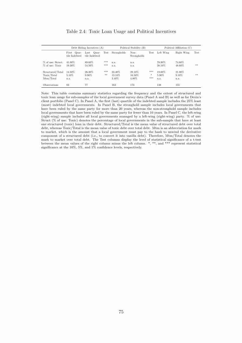
Table 2.4: Toxic Loan Usage and Political Incentives

Debt Hiding Incentives (A) Political Stability (B) Political A�liation (C)

First Quar-tile Indebted

Last Quar-tile Indebted

Test Strongholds Non-Strongholds

Test Left Wing Right Wing Test

% of use: Struct. 41.00% 89.60% *** n.a. n.a. 70.30% 74.60%% of use: Toxic 19.30% 54.50% *** n.a. n.a. 38.10% 48.60% **

Structured/Total 14.50% 26.30% *** 23.40% 29.10% *** 19.00% 21.00%Toxic/Total 5.10% 9.90% ** 13.10% 16.50% * 5.90% 9.10% **Mtm/Total n.a. n.a. 3.40% 4.80% *** n.a. n.a.

Observations 83 77 163 173 138 155

Note: This table contains summary statistics regarding the frequency and the extent of structured andtoxic loan usage for sub-samples of the local government survey data (Panel A and B) as well as for Dexia’sclient portfolio (Panel C). In Panel A, the first (last) quartile of the indebted sample includes the 25% least(most) indebted local governments. In Panel B, the stronghold sample includes local governments thathave been ruled by the same party for more than 20 years, whereas the non-stronghold sample includeslocal governments that have been ruled by the same party for fewer than 10 years. In Panel C, the left-wing(right-wing) sample includes all local governments managed by a left-wing (right-wing) party. % of use:Struct (% of use: Toxic) denotes the percentage of local governments in the sub-sample that have at leastone structured (toxic) loan in their debt. Structured/Total is the mean value of structured debt over totaldebt, whereas Toxic/Total is the mean value of toxic debt over total debt. Mtm is an abbreviation for markto market, which is the amount that a local government must pay to the bank to unwind the derivativecomponent of a structured debt (i.e., to convert it into vanilla debt). Therefore, Mtm/Total denotes themark to market over total debt. The Test columns display the level of statistical significance of a t-testbetween the mean values of the right column minus the left column. *, **, and *** represent statisticalsignificance at the 10%, 5%, and 1% confidence levels, respectively.

75

Table 2.5: Incentives to Hide Cost of Debt

Probit Ordered Probit Magnitude

Structured Structured Toxic Toxic Structured Toxic(1) (2) (3) (4) (5) (6) (7) (8)

Debt/Population 1.564*** 2.081*** 0.751*** 0.679*** 0.812*** 0.817*** 12.831*** 0.021**4.28 4.29 5.07 7.53 4.55 8.07 7.71 4.32

Right-Wing Dummy 0.226*** 0.364 0.223** 0.365*** 0.210** 0.323*** 2.317 0.018*3.56 1.47 2.15 8.05 2.44 3.27 0.79 2.62

Equipment Expenditure/Pop. -0.004*** -0.001* -0.002*** -0.02 -0.000**-3.71 -1.67 -2.88 -2.08 -3.29

Wages/Operating Expenditure 3.809*** 0.965 2.350*** -0.592 0.0065.51 0.94 4.38 -0.04 0.23

Debt Average Maturity 0.075*** 0.057*** 0.083*** 1.204** 0.004**2.99 3.05 4.94 3.65 3.75

Log (Population) 0.070*** 0.085*** 0.082*** 1.110** 0.003**3.56 8.13 18.87 5.5 4.97

Unemployment 0.019 0.046* 0.030* -0.239 0.001**0.84 1.65 1.66 -1.14 3.42

Agriculture 0.003 0.076** 0.039*** -0.914 0.002**0.09 2.33 2.71 -2.19 4.29

Industry 0.047** 0.025 0.039 0.309 0.0021.98 1.53 1.45 0.89 1.83

Lender Relationship FE NO YES NO YES NO YES YES YES

Local Government Type FE YES YES YES YES YES YES YES YES

Pseudo R2 / R2 0.135 0.304 0.065 0.181 0.04 0.129 0.243 0.259

Number of Observations 293 275 293 275 293 275 263 263

Note: This table contains the probit regression coe�cients using debt portfolio data from a sample of localgovernments (Dataset A). The dependent variable is a dummy variable for the use of structured productsfor the first two columns, a dummy variable for the use of toxic loans (as defined in section 2) for columns3 and 4, and a variable covering the 6 levels of underlying risk for columns 5 and 6. Standard errors of thecoe�cients are clustered by types of local governments, and Z-statistics are reported in brackets. *, **,and *** represent statistical significance at the 10%, 5%, and 1% confidence levels, respectively.

76

Table 2.6: Politically Contested Areas

Structured Debt Structured Debt Mark to Market Mark to Market Toxic Debt Toxic Debt/Total Debt /Total Debt /Total Debt /Total Debt /Total Debt /Total Debt

(1) (2) (3) (4) (5) (6)

Years in Power -0.1683* -0.1761** -0.0401** -0.0373** -0.0785* -0.1245***-2.97 -4.94 -5.37 -6.9 -3.1 -9.91

Right-Wing Dummy 1.5221*** 0.0204 2.8585**9.52 0.48 7.3

Log (Population) -5.9739* -0.8441* -3.2835*-3.42 -2.91 -3.37

Local Gov. Type FE YES YES YES YES YES YES

R2 / Pseudo R2 0.1267 0.1603 0.0513 0.0614 0.0507 0.0665

Observations 389 389 389 389 389 389

Note: This table contains cross-sectional OLS regression coe�cients using data from Dexia’s client portfolio(Dataset B). The dependent variable is the measure of structured loan use intensity as indicated in thecolumn header. Years in power refers to the number of years during which the political party of theincumbent (as of December 31, 2009) has been managing the local government. Standard errors of thecoe�cients are clustered by types of local governments, and t-statistics are reported in brackets. *, **, and*** represent statistical significance at the 10%, 5%, and 1% confidence levels, respectively.

77

Table 2.7: Di↵erence-in-Di↵erences Estimation of Election Timing E↵ects

C-logit Structured Trade Placebo C-logit Structured Trade+\- 18 months + \- 12 months + \- 18 months + \- 12 months

(1) (2) (3) (4)

Interaction Pre-Election/Treatment 0.3522*** 0.3350*** 0.0275 0.02622.88 3.28 0.39 0.26

Quarter Fixed E↵ects YES YES YES YES

Regression Type PANEL PANEL PANEL PANELR2 / Pseudo R2 0.0815 0.0545 0.0805 0.0534Number of Periods 12 8 12 8Observations 2741 2741 2741 2741

Note: This table contains the conditional logit (C-logit) regression coe�cients that are estimated using datafrom Dexia’s client portfolio (Dataset B). The dependent variable is an indicator variable of a structuredtrade for a given local government in a given quarter. In columns 1 and 2, the explanatory variable is aninteraction variable between a dummy for the treatment group (local governments having an election atthe end of 2008Q1) and a dummy for the pre-election period. Columns 3 and 4 present a placebo analysisin which the treatment group dummy that is used in the interaction term has been replaced by a dummyon a random sample of similar size; the regressions include individual public entity fixed e↵ects. Standarderrors are clustered by type of public entity. Z statistics are reported into brackets. The time window is18 months before and after the election (the end of March 2008) for columns 1 and 3, and the window is12 months for columns 2 and 4. *, **, and *** represent statistical significance at the 10%, 5%, and 1%confidence levels, respectively.

78

Table 2.8: Herding Behavior in the Borrowing Choices of Politicians

C-logit Structured Trade OLS � (Structured Debt Notional)(1) (2) (3) (4)

# of Active Public Entity in Same Zonethe Previous Quarter

0.0183*** 10.3991***

5.53 3.03

# of Active Public Entity in Same Zonethe Previous Two Quarters

0.0064** 4.3144*

1.91 1.81

Quarter Fixed E↵ects YES YES YES YES

Regression Type PANEL PANEL PANEL PANELR2 / Pseudo R2 0.155 0.1486 0.0101 0.0098Number of Periods 40 39 40 39Number of Public Entities 2741 2741 2741 2741

Note: This table contains the conditional logit (C-logit) and OLS panel data regression coe�cients thatare estimated using data from Dexia’s client portfolio (Dataset B). The dependent variable is an indicatorvariable of a structured trade for a given local government in a given quarter (or semester) for the conditionallogit regressions and the incremental exposure on structured debt entered into by a public entity in a givenquarter (or semester) for the OLS regressions. The explanatory variable is the number of active publicentities in the same geographical zone (county level), which is defined as the number of public entities thathave implemented at least one structured transaction in the previous quarter (or semester). The regressionsinclude individual public entity fixed e↵ects. Standard errors are clustered by type of public entity. *, **,and *** represent statistical significance at the 10%, 5%, and 1% confidence levels, respectively.

79

Chapter 3

Call Me Maybe?

The E↵ects of Exercising Contingent Capital

Adventure is just bad planning. [Roal Admunsen, Explorer]

81

3.1 Introduction

Excess leverage of financial institutions has been a major catalyst of the recent financial

crisis, leading regulators and politicians to largely blame lenient bank capital rules for the

level of leverage achieved by major financial institutions when entering the crisis. The

debate on bank capital regulation, however, has revealed a fundamental policy dilemma.

As advocated by both regulators (Report of the Independent Commission on Banking

headed by Sir John Vickers (2013)) and academics (Admati et al. (2011)), a mandated

drastic increase in bank common equity capital represents the logical answer to the risk of

financial distress that became evident in the years 2007 - 2009, and will help prevent future

bank bailouts by governments. Enforcing these higher requirements, however, is likely to

have unwanted real e↵ects such as credit contraction, as investors are reluctant to provide

banks with additional equity (Jimenez et al. (2013)).1 This reluctance translates also into

industry practitioners fighting against tighter capital regulation (Ackermann (2010)).

Therefore, contingent capital instruments that combine the advantages of both debt and

equity appear as an attractive solution to this dilemna (Flannery (2005); Brunnermeier

et al. (2009); Kashyap et al. (2008), French et al. (2010)). In principle, debt reductions and

improvement in capitalization can also be achieved through ex post debt restructuring,

for instance via debt-for-equity swaps. Contingent capital securities may, however, be

more e�cient at avoiding expensive bank bail-outs from states and help solving debt

overhang issues (Du�e (2010)) without incurring any risk of default or failure of a debt

restructuring plan. Substituting contingent capital to traditional common equity might

allow banks to improve their resilience without incurring the costs of raising additional

equity.2

The purpose of this paper is to assess how e↵ective contingent capital instruments

are in solving financial distress in financial institutions. More specifically, I address the

following questions: When given discretion over the trigger, do financial institutions

use the contingency o↵ered by such instruments in times of stress? How do debt and

equity investors react to contingent capital trigger events? What is the impact of such

contingent capital triggers on the economic performance of financial institutions? A

burgeoning literature on the theoretical analysis of contingent capital instruments has

emerged, with an important focus on trigger incentives and e↵ects (Sundaresan and Wang

(2013), Pennacchi et al. (2011), Martynova and Perotti (2012), Zeng (2012), Flannery

(2010)). To the best of my knowledge there is no empirical study on this topic yet.

1They find that when capital constraints become tighter banks respond by cutting back lending andnot by relaxing the constraint through a new equity issue.

2The literature documents several deviation from Modigliani-Miller such as: equity underwriter‘s fees,under-pricing of the equity issue due to asymmetry of information, and the negative stock price reactionto the announcement of a new issue. For more details, see Eckbo et al. (2007).

82

To answer these questions, I use the widespread issuance of first generation hybrid

bonds and the massive use of their contingent features by European financial institutions

during the financial crisis. Contingent capital instruments are hybrids between debt and

equity: they are issued as debt securities, with coupon payments and stated maturity,

but include clauses that allow their discretionary or automatic conversion into equity-like

claims during periods of stress. Contingent capital is cheaper than equity because of the

tax shield it provides, and because it allows to raise equity only when needed. These

instruments therefore limit the costs associated with equity issuance to certain states of

nature (Bolton and Samama (2012)). Hybrid Bonds are the first generation of contingent

capital instruments, and are known as Trust Preferred Securities (TPS) in the US. These

debt-like securities give the issuer the option to postpone their repayment, potentially for-

ever, therefore removing any roll-over risk. This contingent feature explains the eligibility

of such instruments as regulatory capital, while the interests they bear are tax-deductible.

Hybrid bonds proved to be very popular: worldwide, they amounted to more than USD 1

trillion in 2008. Under the new Basel III standards, regulators are encouraging financial

institutions to issue new forms of contingent instruments such as Contingent Convertibles

(CoCos), with the Swiss and British national regulators even giving specific targets to

their financial institutions. This regulatory stance has led to a recent surge in contingent

capital issuance. Under Basel III standards, total new contingent capital issuance can

represent up to 3.5% of bank risk weighted assets, or around EUR 400bn only for the

largest European banks.

I focus on the European Hybrid Bond market for two main reasons. First, the Euro-

pean market is by far the largest. In 2008, European Hybrid Bonds amounted to EUR

701bn, or 38.3% of European banks’ regulatory capital. More than 80 percent of banks

subject to the EU stress test have issued such hybrid bonds.3 This amount compares to

USD120bn (EUR86bn) of outstanding TPS that year, or 8.7% of US banks total capi-

tal in 2008.4 The di↵erence in market size follows from the larger size of the European

banking sector, as well as the di↵erent regulatory frameworks.5 The second and most

important reason I focus on Europe is because this is where the triggers occurred. While

European financial institutions have massively used the contingent debt relief o↵ered by

their hybrid bonds, American banks hardly, if ever, exercised options embedded in TPS

during the financial crisis. This deviation is likely to come from contractual and institu-

tional characteristics between the two markets.6 Banks such as Citigroup and JP Morgan

3This perimeter includes 91 banks that contribute to systemic risk according to the European BankingAuthority.

4Amount of total capital are from OECD and The Banker.5The US did not apply Basel II standards, whereas European countries did.6Cf. Section 7 for more details.

83

have been using the contingency of their European hybrid bonds, but not the one of their

Trust Preferred Securities.

The paper’s first contribution is to show that European banks have massively taken

advantage of the contingent features of their hybrid bonds during the period 2009 - 2012.

I find that banks used mainly two trigger mechanisms to obtain a contingent debt relief:

maturity extension, and tender o↵er at a discount. Many issuers extended the maturity

of hybrid bonds by not calling them at their first call date. Non-calls lead to an economic

debt relief for issuers who wish to avoid refinancing at a higher cost, or cannot roll-over

due to a liquidity dry-up. In my data, I find that European banks have not called at first

call date a total of EUR 200bn of hybrid bonds. This amount represents 30 percent of

outstanding hybrid bonds, or 11% of European banks’ total capital. Financial institutions

with the lowest capital ratios, who are therefore most likely to su↵er from a binding

regulatory capital constraint, are more inclined to this action. This finding mitigates

the concern that the discretionary nature of the instruments may lead to risk-shifting

behaviors, because financial institutions would renounce to reducing their debt under this

hypothesis. Among the issuers that did not call, some launched simultaneously a tender

o↵er on the hybrid bonds. The tender o↵er is typically implemented at a significant

discount inherent to the change of maturity on a deeply subordinated claim. These

combined actions allow the financial institution to immediately book the o↵er discount

as a capital gain that increases permanently Core Tier 1 capital by the same amount,

leading to a regulatory debt relief.7 Investors have tendered more than EUR 87bn of

hybrid bonds, which allowed banks to book EUR 22bn of capital gain.

The second contribution of the paper deals with investors’ reaction to triggers. Con-

tingent debt relief is, for the most part, received positively by regular debt holders, while

reactions from shareholders are more mixed. The market reaction is more pronounced

for non-calls coupled with tender o↵ers, which is consistent with their e↵ect on Core Tier

1 capital, a key indicator for the regulator during the crisis. Moreover, exchange o↵ers

into equity, which bring the largest e↵ect on debt reduction, are received positively by

both debtors and shareholders.

The third contribution consists in providing empirical evidence of positive and persis-

tent economic e↵ects for banks using contingent capital features. Financial institutions

that obtain permanent debt relief through the exercise of contingent capital provisions

show significantly higher returns on assets, and this relative improvement is proportional

to the increase in Core Tier 1. This e↵ect is robust to controlling for government bail-outs

and seasonal equity o↵erings, and is driven by a more preserved lending activity.

7Core Tier 1 capital, or Common Equity Tier 1 capital, represents the highest quality of Tier 1 capital,meaning that it does not include goodwill and hybrid Tier 1 instruments.

84

Non-calls coupled with tender o↵ers have similar economic e↵ects as recently issued

Write-O↵ Bonds and CoCos : an immediate gain, combined in some cases with an is-

suance of equity. Since regulators and financial analysts focus on regulatory capital, the

impact of debt reliefs on regulatory capital ratios is key for the issuer. The discretionary

nature of the events studied in this paper makes them even more comparable to the form

of contingent capital proposed by Bolton and Samama (2012), Contingent Capital with an

Option to Convert.8 Therefore, my results illustrate how innovative liabilities products

can help ex ante to decrease financial distress costs associated with high leverage.

For the purpose of my analysis, I build a unique and comprehensive database of

European hybrid bond issuances and contingent debt reliefs from 1998 to 2012. I con-

sider as contingent capital instruments any hybrid security classified as Tier 1 or Tier

2 under Basel II that is issued with default debt-like payo↵ terms and includes explicit

option features that allow for an out-of-court transformation of these securities into more

equity-like claims. I hand collect data on debt relief events at the bond level from issuer

announcements and broker coverage reports and match this data with issuer financials,

as well as CDS and share prices. In terms of methodology, I use logit regressions on con-

tingent debt reliefs to identify the type of financial institutions that use the optionality

o↵ered by these instruments. I then implement an event study methodology on hybrid

bond issuer stock and CDS prices to identify the market reaction to contingent debt relief

trigger. I calculate abnormal returns associated to these events for both CDS and stock

price. I explain the cross-section of market reaction through OLS regressions on the type

of contingent debt relief and issuer capitalization. In a following step, I use the same

data on contingent debt reliefs matched with bank financial statements. I implement a

di↵erence-in-di↵erences analysis for measuring the impact of such actions on economic

performance, as measured by return on assets. Although contingent debt relief is discre-

tionary, I limit potential self-selection biases for my treatment group by using a control

group obtained through propensity score matching. The propensity score is calculated

on variables that capture the exposure to regulatory capital constraint.

This paper relates to several fields of the literature. First, this work addresses the

question of bank capital structure (Admati et al. (2011), DeAngelo and Stulz (2013)),

related bank debt overhang (Admati et al. (2012)), and behavior of distressed financial

institutions (Acharya et al. (2013b)). This paper supports contingent capital instruments

as an e↵ective alternative to raising common equity requirements (Du�e (2010)), while

addressing some of the concerns over potential pernicious e↵ects (Sundaresan and Wang

(2013)). Second, this study builds on the knowledge of subordinated debt and Trust Pre-

8These instruments are bonds convertible into shares, where the option to convert belongs to theissuer.

85

ferred Securities in the US (Krishnan and Laux (2005), Benston et al. (2003)), and provide

insights on how contingent capital instruments perform well in practice. Therefore, my

paper suggests another potential interpretation of the results of Boyson et al. (2013):

the lower resilience during the crisis of TPS issuers might come from American banks

not using the contingent features o↵ered by these instruments. Third, my work relates

broadly to financial innovation. An established literature studies the impact of innova-

tive assets such as securitization on bank balance sheets (Loutskina (2011)), but my work

underlines the importance of innovative liabilities. Although some financial innovation

may be driven by adverse incentives (Perignon and Vallee (2014)), contingent capital in-

struments illustrate how more financial innovation can create value (Perez-Gonzalez and

Yun (2013)), and how more innovation on the liabilities side of the balance sheet may

help prevent future financial crises (Haliassos (2012)). In addition, innovative liabilities

can also complement lines of credit to help solving corporate roll-over risk (Acharya et al.

(2013a)).

This paper is organized as follows: Section 2 provides background on the European

market for hybrid bonds and the mechanisms of debt relief, and Section 3 presents the

dataset built for the empirical analysis. Section 4 documents the magnitude of contingent

debt relief and identifies the characteristics of contingent debt relief users. Section 5

provides hypotheses, methodology and results for the study of market reaction to debt

relief, while Section 6 analyses the economic performance of issuers that have triggered

permanent debt reliefs. Section 7 o↵ers a discussion on validity and implications of my

results, and Section 8 concludes.

3.2 Background and Debt Relief Mechanisms

3.2.1 The European Hybrid Bond Market in the Run-up to the

Crisis

In 1998, the Basel committee modified its bank capital rules by clarifying its position con-

cerning hybrid instruments and their eligibility as regulatory capital.9 This announcement

followed an increasing number of innovative hybrid instrument issuances: fixed income

instruments with repayment in 5 to 10 years, which granted them coupon tax deductibil-

ity, but embedding an option to postpone repayment for a very long horizon or even

until perpetuity. This option allows to transform debt-like security into loss absorbing

claims quasi-similar to preferred shares: non-compulsory coupon payments, infinite ma-

turity and no voting rights. The tax deductibility, the absence of covenants, and the

9Source: www.bis.org/press/p981027.htm.

86

non-dilutive nature of these instruments made them an attractive alternative to equity

for banks.

When marketing the hybrid bonds to investors, issuers strongly hinted at their deter-

mination to always honor the call option and to repay the bond in full as soon as the first

call date would be reached. Around 40% of the hybrid bonds also include a commitment

device in the form of a step-up clause: the coupon increases by a pre-determined margin

when the repayment is postponed.10 Calling hybrid bonds at the first call date was the

standard practice before the financial crisis. No exception occurred until the end of 2008,

nor was there any expectation of non-calls, as can be inferred from security prices at

issuance. Thus, Moody’s (2009) writes: “Prior to the financial crisis, there was a tacit

agreement between an issuer and investors that hybrid and subordinated debt would be

called at the first call date”.

Hybrid bonds gained investor interest as they o↵ered higher yields than senior bonds,

due to their junior status that rank them senior only to equity. Fixed income funds were

allowed to invest in hybrid bonds, and hybrid bonds became a popular investment among

fixed income asset managers seeking to increase funds performance.11 Retail investors are

also increasingly attracted to these types of subordinated instruments, as they appreci-

ate the fixed coupon format and the issuers’ reputation. The development of EUR 1,000

denominated bonds, vs. EUR 50,000 and EUR 100,000 denominations targeted at insti-

tutional investors, made it easier for retail investors to access the hybrid bond market.

When assessing financial institutions’ creditworthiness, rating agencies classified hybrid

bonds as equity, which also fostered hybrid bond market development. The market has

met a strong growth since its inception, with issuances rising from EUR2bn in 1998 to

EUR105bn in 2008. Figure 3.1 shows the number of hybrid bond issues by quarter, as

well as their initial maturities if bonds are called at first call date.

INSERT FIG 3.1

However, when the crisis hit and refinancing cost surged for financial institutions,

banks reconsidered their call strategy. The watershed event was on December 16, 2008,

in the midst of the financial turmoil: Deutsche Bank announced that it was not calling

its Lower-Tier II Notes with first call date on January 2009. This first announcement

of a non-call of a hybrid bond took many investors by surprise, and was poorly received

by market operators, with some investors threatening to cease subscription to any future

10A step-up clause typically switch the coupon from fixed rate to variable rate and increases the couponcredit margin by 100 bps after the first call date, which often led to lower coupons than the initial onesduring the financial crisis.

11Deutsche Bank research desk writes “Real money managers are the largest buyers of T1[bonds]”(Bhimalingam and Burns (2011)).

87

debt and equity issuance from Deutsche Bank.12 Following this announcement by one of

Europe’s leading banks, not calling hybrid bonds became increasingly frequent in 2009

and the following years. Despite the initial threats from investors, banks that have chosen

not to call were not sanctioned when raising new debt, as illustrated by Deutsche Bank

following issuance being oversubscribed. Starting in summer 2009, many banks coupled

non-call with tender o↵ers, naming this type of o↵er a Liabilities Management Exer-

cise. By making explicit reference to an impending non-call, banks ensured that bonds

trade at a significant discount, allowing them to make a capital gain on the tender o↵er.13

3.2.2 The Contingent Nature and Regulatory Treatment of Hy-

brid Bonds

Hybrid bonds exhibit a contingent dimension in the sense that the issuer has the option

after the initial non-call period to postpone repayment for a long to infinite amount of

time. The issuer also has the right to defer their coupon without creating an event of

default.14 Both decisions lead to a temporary debt relief, as long as the bond is not

repaid. Appendix A provides an example of hybrid bond terms.

The optional nature of hybrid bonds allows them to gain regulatory treatment as

capital under Basel II. Indeed hybrid bonds account for either Tier I or Tier II capital,

depending on their legal maturity and conditions on coupon payments. Figure 3.2 illus-

trates where hybrid bonds stand in a financial institution balance sheet. For the same

reason hybrid bonds are allowed capital regulatory treatment, they are also considered as

capital by rating agencies, typically with a weight of 50% for Tier 2 securities and 100%

for Tier 1 securities. Under Basel II, banks must hold at least 4% (respectively 8%) of

their risk-weighted assets as Tier I capital (respectively Total Capital, including Tier II

capital). National regulators put a limit on the use of hybrid bonds as part of Tier I

capital, while the Basel Committee puts a 50 % cap on Tier II hybrid bonds as a share

of total regulatory capital. Hybrid capital allows the issuer to meet regulatory capital

ratios at a lower cost than equity for two main reasons. First, hybrid bonds increase the

tax shield as their interests are tax deductible, which represents an important di↵erence

12For instance, Bank of China writes in a letter to every European bank following DeutscheBank decision: “any non-call by a given institution will result in that institution’s debt (not justlower tier 2 but senior and tier 1 as well) being ineligible for future investment consideration”. Source: http://www.independent.co.uk/news/business/news/bank-of-china-furious-at-deutsche-debt-move-1207511.html.

13Explicit reference to non call policy appears in the majority of o↵er announcement. Source: BarclaysResearch.

14For non cumulative securities, issuer has even the right not to pay the coupons without creating anydefault, also such decisions have been extremely rare and typically imposed by the regulator.

88

with preference shares. Second, hybrid bonds are priced ex ante with a high likelihood

of a redemption at first call date, and not priced to their maximum possible maturity, as

would be the case with preference shares. The economic rationale is therefore to provide

capital only when needed, therefore saving the cost of raising equity in the other states

of nature. Additionally, these instruments allow issuers to diversify their investor base,

by tapping institutional and retail bond investors without any voting right dilution.

INSERT FIG 3.2

3.2.3 Contingent Debt Relief Events

Hybrid bonds contains embedded contingent triggers that can be used to provide debt

relief in times of stress. Figure 3.3 displays the di↵erent types of debt relief allowed by

hybrid bonds, and Table 3.1 summarizes the consequent accounting e↵ects.

INSERT FIG 3.3 & TABLE 3.1

Non-Call

Postponing the repayment of a hybrid bond is the simplest way for a financial in-

stitution to reduce debt service. To do so, the issuer only needs to announce that it is

not calling the security at the first call date, and consequently extending it to its legal

maturity, typically perpetual. The issuer can, however, call back every year the hybrid

bond. A non-call represents an economic debt relief, because it reduces the value of debt

while leaving the regulatory capital unchanged.

The numerical example provided in Table 3.1 is based on a EUR1bn Hybrid bond

with 4% coupon and current refinancing cost at 7%. Postponing repayment of this bond

allows savings of (7%�4%)⇥EUR1bn = EUR30m per year, which impacts the Products

and Losses statement. The balance sheet is left unchanged by this debt relief.

Coupling non-call with a tender o↵er

European financial institutions also implement permanent debt relief by simultane-

ously not calling hybrid bonds and launching tender o↵ers on them. The non-call, whether

anticipated or not, typically leads the bond to trade at a significant discount, as investors

become the holder of a deeply subordinated perpetual bond with non compulsory coupons

during a time of stress. The tender o↵er is thus realized at a significant discount which

allows the financial institution to book the di↵erence between nominal and tender price

as a capital gain. The tender gain feeds into Core Tier 1 capital, and transfers wealth

from a↵ected hybrid bond holders to other debtors and shareholders. Precisely measur-

ing the magnitude of this transfer is possible as it corresponds to the accounting gain

89

booked by the issuer as a result of the debt relief. The issuer can o↵er payment in cash

through a cash tender, or in new securities through an exchange o↵er for either senior

notes, stocks or new hybrid bonds. The mode of payment impacts the leverage of the

financial institutions and therefore matters for regulatory capital constraint as detailed

in Table 3.1.

When looking again at our numerical example in Table 3.1, current refinancing cost

value a perpetuity of EUR 4 at 57 cents per euros of nominal, allowing the issuer to rea-

sonably o↵er a tender price of 60 percent of the nominal. Issuer can launch a cash tender

at this price. Then, if fully subscribed, the capital gain is: (100% � 60%) ⇥ EUR1bn =

EUR 400m. The core Tier 1 capital increases by this same amount. However, as the notes

were part of the total capital, their repayment simultaneously decreases total capital by

EUR 1bn, leading to a net e↵ect on total capital of + EUR 400m - EUR 1bn = - EUR

600m. Another possibility for the issuer is to launch an exchange o↵er, for instance into

equity. The exchange is proposed so that it is economically equivalent for the investor to

a cash o↵er at 60 percent of the nominal. Thus, if the issuer’s share is worth EUR 10, the

issuer will propose to give 60 shares for each EUR 1000 nominal bond. In that case, the

capital gain and core Tier I increase is also of EUR 400m, but the action simultaneously

creates EUR 600m of common equity, leaving total capital unchanged.

3.3 Data

For the purpose of my empirical analysis, I build a comprehensive dataset that covers

financial institutions financial statements, CDS, and share prices, hybrid bond issuances,

and contingent debt relief triggers.

I start by compiling a dataset of the whole universe of hybrid issuances in Europe

over the period 1998 to 2012.15 I extract the characteristics of every hybrid bond is-

suance over the sample period from Dealogic DCM Analytics and Bloomberg. I merge

these two sources using each bond unique ISIN identifier. I complement this data with

handcollected information from issuers website and broker reports. I eliminate dupli-

cates and standardize issuance characteristics variables across the di↵erent sources. I

also convert all amounts into Euros. The cumulated volume of issuance in my database

is EUR826bn. The dataset represents an extensive coverage of the market with for in-

stance a scope of more than 90% of all outstanding hybrid bonds in 2007, as reported by

15European countries included in the analysis: Austria, Belgium, Cyprus, Denmark, Finland, France,Germany, Greece, Hungary, Iceland, Ireland, Italy, Luxembourg, Netherlands, Norway, Portugal, Slove-nia, Spain, Sweden, Switzerland, United Kingdom.

90

the Committee of European Bank Supervisors (CEBS) in 2007. Key issuance variables

includes issuer name, country, security issue date, maturity, coupon, date of repayment

postponement option, and Basel II tier of capital.

I then hand collect press releases from issuers and reports from bank research desks

indicating that issuers have not called at first date a given hybrid bond issue. I also

compile cash and exchange tender o↵er announcement and result releases. For each

o↵er, I collect from these public releases the o↵er date, price, payment type (cash, senior

debt, subordinated debt, new hybrid or equity), the amount tendered, and calculate the

consequent accounting gain. I merge this information with the issuance characteristics

using each hybrid bond ISIN code. I also merge this issuance level dataset with hybrid

bond secondary trading prices with the same identifier. Some non-call events and tender

o↵ers may not be included in this study. I limit this concern by comparing my events list

with the ones published by bank research teams, and typically have a larger sample.16

Furthermore, not including some events can only bias against finding treatment e↵ects,

as some treated financial institutions would be mistakenly included in the control group.

As required for my event study and economic performance analysis, I associate the

issuance level data gathered in the previously described steps with issuer level data. I

proceed as follows. I manually identify subsidiaries and SPV issuers with their holding

company. I then collapse key hybrid bond and debt relief data at the holding company-

year level, using name and country as an identifier.

I then merge manually by name and country the contingent debt relief data with

issuer senior and subordinated CDS spreads and stock prices from Datastream. Finally, I

integrate balance sheet information from Bankscope through another manual merger by

name of holding company. I convert variables of interest of Bankscope into euros.17 This

process results in a unique and reliable dataset that covers debt relief events, issuance

characteristics, issuer financials, as well as related security prices.

3.4 Contingent Debt Relief Use

Gauging the Use of Contingent Debt Reliefs

Both hybrid bond issuance and recourse to contingent debt reliefs have been widespread

during the sample period. Table 3.2 presents summary statistics on these two phenom-

ena. Column I provides summary statistics on the use of hybrid bonds in Europe. The

sample includes all Tier 1 and Tier 2 hybrid issuances between 1998 and 2012. I exclude

16For instance, Morgan Stanley (2012) lists 25 large European institutions that have not called someof their hybrid bonds.

17I only keep variables from Bankscope with a su�cient coverage and reliability, which I cross-checkon a subsample of annual reports.

91

bullet Lower Tier 2 instruments from the study as they do not embed any optionality.18

The European cumulated issuance amount of EUR826bn compares to issuances of TPS of

USD185bn in the US over the 1996 - 2012 period (Boyson et al. (2013)), making Europe a

much larger hybrid bond market. In my sample, 454 issuers use contingent hybrid instru-

ments. Out of these 454 issuers, 167 have exploited the contingency of these instruments

over the sample period by not calling them at first call date, while 85 issuers implemented

permanent debt relief by coupling non-calls with tender o↵ers. In total, non-calls cover

more than EUR210bn in notional amount, while related tender o↵ers have allowed issuers

to book more than EUR22bn of immediate profit. These figures illustrate how European

financial institutions have been making significant use of the possibility of debt relief of-

fered by these instruments. Issuers have used the di↵erent debt relief mechanisms, some

choosing not to call, some not to call and tender for cash, and some not to call and

tender for other securities. The exact list of debt relief events and summary statistics for

security prices and issuer financials is available in the online appendix.

INSERT TABLE 3.2

Characteristics of Contingent Debt Relief Users

Table 3.3 presents the result of logit regressions on implementing contingent debt

reliefs, for both non-call and tender o↵ers. The left hand side variable in the regressions

is a dummy equal to one if the issuer has implemented during the sample period: a non

call for columns (A) to (C); a non call coupled with a tender for columns (D) to (F). The

analysis is conducted on a single cross-section, with financial data as of 2008, immediately

prior to the first occurrence of contingent debt relief. These regression coe�cients show

that Tier 1 ratio, the most scrutinized regulatory capital ratio, is negatively correlated

with the likelihood of implementing both types of debt reliefs: non call and tender o↵ers.

Contingent debt relief is therefore more widespread among under-capitalized financial

institutions. These banks thus try to maintain or increase their amount of capital. This

points towards financial institutions not engaging in risk-shifting when taking the decision

to, or not to, implement a debt relief. Another important driver of the contingent debt

relief decision is to be under fair value accounting for liabilities. The sign of the coe�cient

on the dummy for using this accounting choice di↵ers according to the type of debt relief.

Having liabilities fair value accounting increases the likelihood of not calling hybrid bonds,

but decreases the likelihood of implementing tender o↵ers. An immediate explanation

is that institutions that have made this accounting choice at issuance do not need to

launch a tender o↵er to book the decrease in value from their hybrid bonds as Core Tier

18So-called bullet Lower Tier 2 are subordinated bonds without any call feature.

92

1. Overall, these results suggest that risk-shifting does not play a dominant role in the

financial institutions decisions regarding contingent debt reliefs. The possible negative

signal of triggers, as well as fear of reputation damage resulting in a higher cost for future

issuances, are likely candidates for explaining that a large share of banks still called their

hybrid bonds at first call date.

INSERT TABLE 3.3

Figure 3.4 compares the amount of issuance and triggered securities by sector. This

comparison helps understanding the motivation for two reasons. First insurance compa-

nies have similar regulatory capital constraints as banks, but have low need of funding.

Insurers traditionally have a long position in cash due to the collection of insurance pre-

mia, and are even forbidden to borrow in some countries. Corporates on the other side,

have funding needs but no regulatory constraints. Figure 3.4 shows that while hybrid

bond issuances have been significantly larger for banks than for insurance and especially

corporate, the fraction of triggered instrument is also much higher than for any of the

other two categories. Trigger are almost non existent for corporation. This graphic

evidence is consistent with regulatory capital being an important driver of the trigger

decision.

INSERT FIG 3.4

3.5 Market Reaction to Contingent Debt Relief Events

3.5.1 Hypotheses

I consider three main frameworks to analyze market reaction to contingent debt relief

triggers: Regulatory Capital Constraint, Signaling, and Risk-Shifting. Table 3.4 summa-

rizes the predictions on debt and equity value for the three hypotheses developed below.

A. Regulatory Capital Constraint: A contingent capital trigger helps releasing a

binding regulatory capital constraint, and hence may allow to finance additional projects

with a positive net present value.

Banks need a minimum of book capital ratio to be able to conduct risky lending and

investing. When undercapitalized, financial institutions can be forced by the regulator

to forego positive NPV projects. Financial analysts also focus on these indicators when

assessing the strength of a bank. As seen in Section 2, triggering contingent debt re-

liefs answers this issue by providing banks with additional regulatory capital. Bolton

93

and Samama (2012) considers contingent capital instruments that provide financial in-

stitutions with an insurance on regulatory capital to limit financial distress costs. This

form of contingent capital is highly comparable to the debt reliefs event of this study,

as its trigger is also discretionary to the issuer. Contingent capital increases firm value

by releasing the capital constraint at a cheaper cost than equity, as the cost of raising

equity is born only when needed. Furthermore, underpricing due to information asym-

metry is limited as the issuance occurs several years before the potential distress. The

increase in firm value obtained thanks to the trigger should translate into a tighter CDS

spread and an increase in the stock price. In the case of equity issuance, the positive

stock price reaction also illustrates that new equity is issued at a price below market

price. Finally, the reduction of regulatory capital constraint should facilitate the funding

of risky activities such as lending, which should be observable through an expansion or a

lower reduction of the balance sheet compared to non treated financial institutions. This

improvement should translate into a relatively higher economic performance after banks

trigger contingent capital. Although economic debt overhang may also be at play, and

should be impacted by non-calls, which decrease the market value of hybrid debt, I focus

on the regulatory capital constraint for two main reasons. First, the discussion about

regulatory capital is at the heart of this study. Second, non-calls typically occur for one

issue at a time, whereas a tender o↵er covers multiple issues at the same time, making

the potential e↵ect larger and therefore easier to identify.

B. Signaling: The use of a contingent capital trigger may act as a negative signal by

revealing bad private information about the bank’s financial situation.

Markets may interpret debt relief announcement as a negative signal on bank financial

health and balance sheet quality. Investors can infer from the use of contingent capital

options that managers have negative private information that was not yet incorporated

in the market prices. The overall e↵ect on the bank value is then expected to be negative,

leading Credit Default Swaps spreads to widen and stock prices to decrease. Current and

future economic performance measures should then be negatively correlated with debt

relief, identifying a strong selection e↵ect.

C. Risk Shifting: The use of a contingent capital trigger may decrease risk-shifting

incentives by realigning shareholder incentives with the ones of debtholders.

Due to their high leverage, financial institutions are inclined to risk-shifting (Acharya

et al. (2013b), Landier et al. (2011)). Under this framework, managers have an incentive

to implement high risk projects with negative present value, as long as their pay-o↵s are

su�ciently increased in some states of nature. Exercising a contingent debt relief, when

94

it leads to a decrease in leverage, decreases future risk-shifting incentives. Managers

of highly levered financial institutions may therefore forego the use of contingent debt

relief triggers, despite the increase in firm value it would allow. If risk-shifting is not

at play, discretionary and automatic contingent capital instruments should yield similar

e↵ects: the trigger of a contingent debt relief may lead to a decrease in equity value,

that corresponds to a drop in future risk-shifting opportunities. On the other hand, debt

value should increase as the likelihood of default decreases.

INSERT TABLE 3.4

Type of Contingent Debt Relief

Finally, the type of contingent debt relief should also matter for the valuation e↵ects.

When compared to all types of debt relief, market reaction and economic performance

should be more positive for a debt relief that is permanent, cash neutral, and associated

with equity issuance. First, tender o↵ers should have a more pronounced e↵ect than

non-calls, as permanent debt reliefs allow issuers to gain the cumulated present value

of refinancing savings and directly impact the capital ratios. Moreover, a change in

market conditions or regulatory treatment might a↵ect the value of non-called hybrid

bonds and might lead issuers to end them, making their total benefit uncertain. Second,

leverage neutral or improving transactions, such as exchange o↵ers into equity or hybrid

bonds, should lead to more positive e↵ects than the ones that increase leverage and

regulatory capital constraint, such as cash tenders or exchange into senior debt. These

e↵ects may vary according to the level of leverage of the considered financial institution.

Third, exchanges into equity should better solve the regulatory capital constraint: by

simultaneously transferring value from hybrid debt holders while raising capital, these

transactions improve the most Core Tier 1 capital, while limiting dilution costs.

3.5.2 Event Study

I study the market reaction for both bondholders and shareholders by implementing an

event-study methodology (Brown and Warner (1985) and MacKinlay (1997)). I analyze

the impact of all debt relief, and then focus on permanent debt relief only. I use CDS

spreads to measure debt value reaction because CDS are more liquid than bonds. For the

equity value reaction, I examine stock prices.19 If assuming semi-strong form e�ciency,

market reaction is only driven by information made public at the time of the debt relief

announcement. Although a small number of debt relief announcements were made in con-

junction with other issuer specific news, the large majority of debt reliefs was announced

independently from any other corporate events, as observed on issuer press releases.

19This methodology is used for instance in Jorion and Zhang (2007).

95

Table 3.5 presents the mean cumulative adjusted returns of CDS and the mean cu-

mulative abnormal returns of stock price to debt relief events. Panel A covers all non-call

events, Panel B shows non-calls coupled with tender o↵ers, and Panel C focuses on non-

calls coupled with exchange o↵ers only. I calculate adjusted returns of CDS as the change

in a given issuer spread minus the change in its benchmark index. The benchmark index

is the iTraxx Financial Senior for the senior CDS and the iTraxx Financial Sub for the

subordinated CDS. This adjustement is comparable with the rating adjusted spread used

in Jorion and Zhang (2007). Stock abnormal returns are calculated based on the CAPM

model, using Eurostoxx 50 as the market index. Stock betas are estimated prior to the

debt relief events, over a window of 200 days starting on the January 1, 2008.20 Cumu-

lative abnormal returns are the sum of abnormal returns over the considered windows:

daily, over -1/+1 days, and over -2/+2 days. Panel A presents the results for senior CDS,

Panel B for Subordinated CDS, and Panel C for stock prices.

INSERT TABLE 3.5

Positive Credit Market Reaction

Table 3.5 shows that debt relief events have a tightening e↵ect on issuer CDS spreads,

meaning investors perceive issuer credit quality to be improved. The e↵ect on issuer CDS

spread is statistically and economically significant for the subordinated CDS. Senior CDS

spreads present the same tightening reaction, but results are not significantly di↵erent

from zero. The larger magnitude of subordinated CDS reaction is consistent with these

securities being more information sensitive than senior CDS, and less influenced by too-

big-to-fail government put options. The tightening e↵ect is stronger when restricting

the sample to non-calls associated with tender o↵ers, with a significant decrease in the

spread of 9 bps on the announcement day. These results are robust to the time window

considered, with the coe�cient having the same sign and magnitude for 3 and 5 days

windows. These e↵ects are unlikely to be driven by liquidity, as bank CDS are typically

more liquid than corporate CDS. Tender o↵ers might however decrease the liquidity of

some underlying bonds. Such an e↵ect would bias against finding a tightening reaction, as

a decrease in liquidity would widen the CDS spreads. This positive credit market reaction

is consistent with both hypotheses of regulatory capital or risk shifting reduction, but

not with a negative signaling e↵ect.

Panel A of Table 3.6 examines the reaction by type of contingent debt relief: a non-

call, a permanent relief through a cash tender o↵er, or a permanent relief through an

exchange o↵er. I estimate the following model:

20Results detailed below are robust to using stock adjusted returns, calculated by subtracting thebenchmark index performance to the stock performance.

96

Adj CDS Deltai,t

= a + b.Type of Debt Reliefi,t

+ c. Bank Characteristicsi,t

+

Subordinated CDS Dummyi

+ Quarter FEt

+ ei,t

where Adj CDS Delta is the CDS adjusted return, and Type of Debt Relief are dummy

variables for permanent debt relief, cash tender, and exchange o↵er. The control group

therefore comprises non-call-only events, on the day of notice of the decision. Standard

errors are clustered by issuer.

Results are shown in columns (A) to (C) of Panel A in Table 3.6. Among all debt

reliefs, permanent debt reliefs have a strong tightening e↵ect on the CDS spreads. Cash

tenders have the same tightening e↵ect on CDS spreads. The situation is more heteroge-

nous for exchange o↵ers. I use leverage defined as total assets over total regulatory capital

as an empirical proxy for regulatory capital constraint. By interacting the exchange o↵er

dummy with leverage, I find that exchange o↵ers lead to spread tightening in general,

but to a CDS spread widening for highly levered institutions. To interpret this result, I

need to discriminate by the type of security provided in the exchange, as the e↵ect on

leverage varies according to the type of exchange o↵er.

INSERT TABLE 3.6

Therefore in a next step, I restrict the sample to exchange o↵ers, and study the

reaction by type of securities o↵ered in the exchange. I use exchange into hybrid debt

as a control group. These regressions include controls for o↵er price and size. Standard

errors are again clustered by issuer. The precise specification of the regressions conducted

on the small subset of exchange o↵ers is:

Adj CDS Deltai,t

= a + b.Type of Security exchanged intoi,t

+ c. Bank Characteristicsi,t

+ Subordinated CDS Dummyi

+ O↵er Characteristic Controlsi,t

+ Quarter FEt

+ ei,t

Results are displayed in columns A and B of Panel B in Table 3.6. An exchange into

equity leads to the stronger tightening e↵ect, while the impact of an exchange into senior

is not significantly di↵erent from zero. However, when interacting with leverage, I find

that exchange into senior debt leads to a tightening of the CDS spread for low leverage

institutions, but to a widening of CDS spreads for highly levered institutions. This credit

investor reaction is consistent with a poor perception of triggers that actually increase

leverage for highly levered financial institutions, as it potentially drives up regulatory

capital constraint or risk-shifting incentives.

Overall, the CDS spread reaction is consistent with the hypotheses that debt relief

helps reduce both regulatory capital constraint and risk-shifting incentives, as credit qual-

ity is perceived as improved by market participants. More specifically, markets seem to

97

validate transactions that have permanent e↵ects. Consistent with reducing regulatory

capital constraint, exchange into equity is positively received by debtors. In the next

subsection, I study equity reaction to disentangle regulatory capital constraint from risk-

shifting.

Reaction of Stock Prices

Stock market reaction to a contingent debt relief trigger di↵ers according to the type

of the debt relief. Overall, share prices appear to react negatively to the trigger events,

as illustrated by Panel C of Table 3.5. However when looking at the cross-section of stock

reaction by type of debt relief in Table 3.6, I observe that exchange o↵ers receive a more

negative reaction than non-calls and cash tender. When adding an interaction between

the type of debt relief and the level of leverage, I observe the following. First, cash tender

o↵ers are positively received for low leverage financial institutions. When implementing

these transactions, issuers face the following trade-o↵: improving their Core Tier 1 capital

at the cost of decreasing their total regulatory capital. Negative stock market reaction

for high levered issuers points towards the decrease in total regulatory capital being too

costly for this type of issuer. Second, the level of leverage does not seem to impact the

reaction to exchange o↵ers, as interacting the exchange o↵er dummy with the level of

leverage does not yield significant results.

As I did for CDS spreads, I restrict my event sample to exchange o↵ers in panel

B of Table 3.6. Similar to CDS spread reaction, stock price reaction is significantly

higher for exchange into stocks, when compared to exchange into subordinated securities.

Exchanges into senior debt do not yield an e↵ect significantly di↵erent. It is unusual

to observe a positive reaction to equity issue, as it typically leads to dilution. The

specific design of this contingent debt relief, that allows to simultaneously book a capital

gain, might explain this result. Economic magnitude of this result is high, but must

be interpreted with caution due to the limited number of observations. Also, I cannot

interact with leverage in this specification due to the size of the considered subset.

Overall, the stock price reaction is consistent with contingent debt relief decreasing

risk-shifting incentives, and therefore decreasing equity value. Exchanges into equity,

however, lead to an increase in both debt and equity value, which suggests that this relief

helps relax the regulatory capital constraint. This result validates the relevance of an

instrument that o↵ers simultaneously an immediate gain in time of distress while raising

some additional capital, and represents a rare occurrence of well received equity issuance.

98

3.6 Economic E↵ects of Contingent Debt Relief

3.6.1 Impact on Economic Performance

I estimate the e↵ects of debt relief events on economic performance in a di↵erence-in-

di↵erences set up. I focus on permanent debt reliefs as their e↵ect on the P&L statement

and balance sheet is larger and more persistent. However, I also control for temporary

debt reliefs in my analysis. The treatment consists of permanent debt reliefs that oc-

curred between 2009 and 2011. I use three di↵erent control groups of untreated financial

institutions: first, all hybrid bond users for which financial data is available in Bankscope,

which corresponds to financial institutions that were in a position to implement perma-

nent debt reliefs, second, all financial institutions that used non-calls, and finally the

financial institutions that have implemented permanent debt reliefs in 2012, but not be-

fore. Summary statistics of key financial variables are presented for the di↵erent subsets

in the Appendix.21 I estimate the following model on yearly financial data ranging from

2007 to 2011:

Return on Assetsi,t

= a + b. Post⇥ Treatedi,t

+ c. Treatedi

+ d. Bank

Characteristicsi,t

+ Year FEt

+ ei,t

where Treated is a dummy variable for having a debt relief in any year, Post⇥ Treated

a dummy variable for having a debt relief during this given year or a previous year. I

control for not calling hybrid bonds and seasonal equity o↵ering with dummies for such

events. Regressions also include controls for previous accounting exercise total assets,

Tier 1 capital ratio, impaired loans over equity, amount of hybrid bond, client deposits

over total funding, risk weigthed assets over total assets, and yearly change in total assets,

as well as a dummy variable for being publicly listed, and year fixed e↵ects. Standard

errors are clustered by issuers.

Results are presented in Table 3.7. Permanent debt relief is associated with a higher

economic performance. The positive and significant coe�cient on the dummy for per-

manent debt relief shows that these actions have a positive impact on return on assets

(ROA). This result is robust to a battery of controls, and holds for all three control groups.

This e↵ect is economically significant: regression coe�cients indicate an improvement of

ROA between 0.6% and 1.0% according to the control group.

To confirm the validity of this result and limit concerns over unobserved variables to

factors correlated with the size of the relief, I then interact post⇥treated with the capital

gain obtained through the debt relief, as a percentage of total assets:

21Banks from the treatment group are on average larger and more frequently listed than for the controlgroup

99

Return on Assetsi,t

= a + b1. post⇥ treatedi,t

+ b2. post⇥ treated⇥ gaini,t

+ c.

treatedi

+ d. Bank characteristicsi,t

+ Year FEt

+ ei,t

Results appear in columns (B), (D) and (F) of Table 3.7 for the three control groups.

The larger a permanent debt relief, the more it impacts the ROA of the a↵ected financial

institution. Again, a battery of controls, year fixed e↵ect for example, also leaves the

coe�cients of interest significant. This coe�cient mitigates concerns that unobserved

variables are driving the previous results, as these variables need to be correlated with

the size of the capital gain obtained through the contingent debt relief.

This higher economic performance for financial institutions that implemented per-

manent debt relief is consistent with the initial hypothesis that these actions help relax

the regulatory capital constraint. By providing a gain in di�cult times and allowing

financial institutions get adequate capitalization when needed, debt relief can help avoid

discounted fire sales or renouncing to positive NPV projects.

Moreover, the positive correlation between debt relief and economic performance

makes reverse causality unlikely to drive the result. If at play, potential endogeneity

would go against finding positive e↵ects of debt relief, as the capital gain relates to how

discounted hybrid bonds are, and therefore to how distressed the financial institution is.

Therefore, potential self-selection would bias the treatment group towards having more

banks in financial trouble than in the control group, which makes them consequently un-

likely to exhibit relatively higher economic performance. Controls for key financial ratios

should also limit this concern to unobserved variables. I further address and discuss the

self-selection issue in the next section.

The coe�cient on the dummy for hybrid bond non-call is negative and highly signif-

icant. Here this result is likely to be driven by a reverse causality e↵ect: as shown in

section 4, financial institutions use their temporary contingency when distressed, which

makes it challenging to identify the real e↵ects of this action. A potential treatment e↵ect

of non-call does not seem to dominate the selection e↵ect. Seasonal equity o↵erings do

not appear to be significantly correlated with economic performance measured as return

on assets. Controlling for the change in balance sheet size is important to make sure

that the improved economic performance is robust to asset sales, and does not come from

concentrating operating income on a smaller asset base.

INSERT TABLE 3.7

3.6.2 Inspecting the Transmission Mechanism

Understanding the channel through which contingent instruments improve economic per-

formance is key for assessing their relevance and e�ciency. If these instruments help

100

reduce regulatory capital constraint, financial institutions that have triggered debt reliefs

should exhibit a smaller decrease in lending, as well as a higher performance of this ac-

tivity. Reducing the regulatory capital constraint should allow financial institutions to

finance relatively more positive-NPV projects. Using the same set up as in Table 3.7, I

test these predictions by looking at the impact of contingent debt reliefs on the asset side

of the balance sheet and on interest income. I estimate the following specification:

Y(i,t) = a + b. post⇥ treated + c. treated + other events control + Bank

characteristics(i,t) + year FE (t) + e(i,t)

where Y(i,t) is successively log(Loans), Risk-Weigthed Assets over Total Assets, and

Interest Income over Total Assets. I consider two control groups: hybrid bond issuers,

and non-call users.

Table 3.8 displays the results. Contingent debt relief appears to impact the quan-

tity of loans retained. When looking at asset composition, I find that treated financial

institutions keep a higher ratio of risk weighted assets over assets. These results show

that, on average, treated financial institutions stay more invested in risky assets during

the financial crisis. This di↵erence in asset composition translates into higher interest

income, as exhibited by the positive and significant coe�cient on Post ⇥ Treated in

columns (C) and (F). These e↵ects are robust to restricting the control group to non-call

users. Altogether, these results corroborate the role of contingent debt relief in relaxing

the regulatory capital constraint and its pernicious e↵ects on lending in times of distress.

INSERT TABLE 3.8

3.7 Discussion

3.7.1 Alternative Hypotheses

Self-selection

A natural concern about comparing the economic performance of contingent debt relief

users with the one of a control group is the self-selection bias. Conditionally on hav-

ing issued hybrid bonds, financial institutions decide themselves to be treated due to

the discretionary design of the trigger. This decision might be correlated with impor-

tant variables that drive economic performance. To address this concern, I implement a

propensity score matching to alleviate self-selection concerns. This high comparability

comes however at a cost of a somewhat lower statistical power, as it decreases the sample

size. The propensity score matching methodology allows to rule out endogeneity on past

101

observable variables included in the logit analysis of the propensity score. This set-up

therefore restricts endogeneity concern to unobserved time-varying variables.

Table 3.9 presents the same specifications as Table 3.7 and Table 3.8, with the control

group built by using propensity score matching. The propensity score is calculated on the

following variables with their 2008 value: total assets, Tier 1 capital ratio, client deposits

over total funding, impaired loans over assets, risk weigthed assets over total assets, yearly

change in total assets, as well as a dummy variable for being publicly listed. I take the

closest five non-treated financial institutions for each treated financial institution, with

possible replacement to maximize comparability. These replacements happen frequently,

which explains the small size of the control group.

Both economic performance and balance sheet composition e↵ects are confirmed by

this additional robustness test. I use return on assets, log(Loans) and Risk Weighted

Assets over Total Assets as left hand-side variables. The coe�cient on the interaction

dummy Post⇥Treated is significantly positive in all three specifications. The coe�cient

on the triple interaction terms post⇥ treated⇥ gain in column (B) also bears a positive

coe�cient, which reinforces the validity of the result, as unobservable variables need to

be correlated both with treatment timing and size to create endogeneity.

INSERT TABLE 3.9

A change in regulatory framework that fostered tender o↵ers from mid 2010 mitigates

endogeneity concerns on unobserved variables. As part of the Basel III standards im-

plementation, the Basel Committee on Banking Supervision’s announced on September

10, 2010 new standards for hybrid instrument to be included in regulatory capital.22 For

the vast majority, existing hybrid bonds did not comply with these new standards. This

regulatory change led to an increase in the incentive to repurchase or exchange existing

bonds for issuers, as opposed to only postponing their repayment. When a hybrid bond

loses regulatory capital classification, it becomes less attractive for the issuer. This shock

covers all financial institutions and therefore cannot be convincingly used in a di↵erence-

in-di↵erence setting or an instrument variable analysis. However, its regulatory nature

supports a significant exogeneity of the trigger for permanent debt relief to the bank

unobservable characteristics. Tender o↵ers are significantly more frequent after the reg-

ulatory change than before.

22The main requirement announced was to increase the loss absorption mechanism of hybrid instru-ments, namely by making nominal write-o↵ or conversion into equity automatic below a pre-specifiedtrigger, and to avoid any incentive to redeem the securities prior to their maximum maturity.

102

Government Bail-Outs

Several financial institutions that implemented contingent debt relief also benefited from

government bail-outs. An alternative hypothesis is therefore that the observed positive

e↵ects of debt contingent relief on economic performance may be driven by the subsam-

ple of banks that benefited from government bail-outs. A capital injection from taxpayer

money, while potentially creating governance issues, may help reduce the regulatory cap-

ital constraint.

To rule out this alternative explanation, I conduct the same OLS analysis as in Table

3.7, keeping the variables related to contingent debt relief, but I add a dummy for banks

that were beneficiaries of a government-sponsored bail-out (henceforth, the bailed-out

banks), as well as an interaction between being a bailed-out bank and being post bail-

out. The online appendix shows the list of bailed out banks obtained from the European

Commission website, that includes all financial institutions that have been the object of

an individual aid. 23

Table 3.10 shows that the positive e↵ect of debt relief is robust to this additional

control. I use the same control groups as in section 6. Column A corresponds to the

control group of hybrid bond user, column B to non-call users and column C to the

control group that implemented contingent debt relief post sample period. While the

selection e↵ect appears to be strong for bailed out banks, with a significant negative

coe�cient on the dummy for bail-out, the treatment e↵ect identified on the interaction

term is not significantly di↵erent from zero. This compares to the opposite results for

contingent debt relief: no apparent selection e↵ect, but a significant treatment e↵ect. The

association of improved economic performance with contingent debt relief is therefore

robust to controlling for government bail-outs.

INSERT TABLE 3.10

Country e↵ects

Debt reliefs are more frequent in some countries than others. The positive e↵ect of debt

relief triggers may come from di↵erence in trends between countries within Europe, which

are unrelated to the events I am studying. Sovereign risk and state of the economy are the

usual suspects. Countries from the periphery of the Euro-zone, such as Portugal, Italy,

Ireland, Greece and Spain have been facing both an important risk of default from their

central government and a fragile health of their economy. Scandinavian countries, on the

other side, have been partly immune to the economic crisis and the related sovereign debt

turmoil. To rule out this explanation, I include in the main specification of my analysis

of economic performance dummies for these two geographic zones, that I interact with

23Source: http://ec.europa.eu/competition.

103

year fixed e↵ects. Table 3.11 shows that the positive impact of debt relief remains valid

in this robustness check.

INSERT TABLE 3.11

3.7.2 Comparison with Second-Generation Contingent Capital

Instruments

A parallel can be drawn between the two types of permanent debt relief and the two

most discussed forms of contingent liabilities. Cash consuming debt relief is economically

similar to write-o↵ bonds, as it allows to book an immediate gain while having to provide

only a fraction of bond nominal in cash to investors.

Permanent debt reliefs through an exchange o↵er are comparable to Contingent Con-

vertibles (CoCos), as the immediate gain at trigger comes with the remaining fraction

of nominal being exchanged into new securities, possibly stocks. On top of their dis-

cretionary nature, permanent debt reliefs di↵er from write-o↵ bonds and CoCos to the

extent that the investor can choose not to subscribe to the o↵er. Except for certain o↵ers

under Dutch auction format where it was not possible to infer the o↵er price, investors

have largely subscribed to tender o↵ers. A likely explanation is that investors were eager

to use the liquidity they provided. Indeed, another important di↵erence between the

first-generation instruments, hybrid bonds and TPS, and the second generation is one

of investor perception: while post-crisis investors cannot be mistaken about the bail-

in design of their contracts, investors buying hybrid bonds prior to the crisis arguably

may have been under the impression that they had bought plain-vanilla bonds. Retail

investors in Spain and UK are currently suing banks for product mis-sellling, following

investor losses due to non-calls and tender o↵ers at a discount.24 Finally, the main dif-

ference with CoCos lies in the discretionary nature of the studied debt reliefs. However,

the results of section 4 indicates that risk-shifting is a limited concern. Therefore, the

conclusion of this study should hold for automatic instruments when regulatory capital

constraint, and validates the regulator positive stance towards CoCos. Furthermore, the

results of this paper are supportive of the contingent capital design proposed by Bolton

and Samama (2012). Multiple equilibria issues and external manipulation are less of a

concern for discretionary instruments.

24Source: http://nyti.ms/14Z08ke.

104

3.7.3 Comparing Europe and the United States

During the recent financial crisis, American banks triggered significantly less debt relief

than European ones. Trust Preferred Securities have been largely called at first possible

date despite the di�culties of American financial institutions. In contrast to European

hybrid bonds, many US hybrid bonds were trading above par, fostering issuers to use the

regulatory call clause to call these bonds at par and refinance with cheaper securities.25

The regulatory calls were made possible by the implementation of the Dodd Frank Act,

which changed the regulatory treatment of TPS securities. The majority of US bank trust

preferred securities traded above par due to bail-out guarantees and a more protective

legal documentation. TPS are cumulative and include a dividend stopper clause, meaning

that US investors are better protected against non payment of coupon and principal

than European ones.26 This e↵ect, combined with a sharper decrease in interest rates is

likely to have limited TPS trading discounts. Although permanent debt relief through

extension coupled with tender o↵ers seems very limited (Boyson et al. (2013)), there exists

evidence of some use of open market purchase, as well as extension of a minority of trust

preferred securities.27 American banks such as JPMorgan or Citigroup have been steadily

calling their USD denominated Trust Preferred Securities, while not calling their EUR

denominated hybrid bonds. This decoupled strategy could also be driven by reputation

concerns.

New TPS in the US are non-cumulative and should therefore behave more similarly

to European ones. Would a su�cient amount of debt relief be identified in the US, the

results of the paper should also hold for the US market.

3.8 Conclusion

This paper explores the European hybrid bond market to analyze the market reactions

and economic e↵ects of contingent capital triggers by financial institutions. While the Eu-

ropean Sovereign Crisis and its e↵ect on the banking sector has been under the spotlight

for several years, the episode of non-calls and tender o↵ers by European banks has drawn

little attention. I document that financial institutions largely triggered the contingent

features embedded into their hybrid bonds during the financial crisis, by not calling their

25The regulatory call clause allows issuer to call at any time at par if the instrument loses regulatorycapital treatment. This clause is present in the documentation of all Trust Preferred Securities andhybrid bonds.

26Cumulative coupons means that any skipped coupons are accumulated to be paid in the future, atthe latest at redemption date. Under a dividend stopper, the issuer cannot for a specified period of time,usually known as the stopper period, pay a coupon on another security or class of securities, typicallystocks, if it does not pay a coupon on the security in question.

27http://seekingalpha.com/article/515731-is-your-preferred-stock-about-to-be-called

105

hybrid bonds at first call dates, and by simultaneously launching tender o↵ers at a dis-

counted price. The likelihood of using their contingent capital discretion appears higher

for highly levered financial institutions, which makes risk-shifting behavior on that aspect

unlikely. When conducting an event study on the dates of announcement of contingent

debt relief, I find that CDS spreads tighten significantly. This increase in debt value is

likely to be driven by a reduction of regulatory capital constraint. The reaction of stock

prices is more mixed depending on the type of relief, but is consistent with a reduction in

risk-shifting incentives. Exchanges into equity, however, are positively received by both

debtors and shareholders, which is again consistent with reducing the regulatory capital

contraint.

Moreover, contingent debt reliefs are associated with higher economic performance,

and better preserved lending activity from their users. This result is robust to controlling

for government bail-out and seasonal equity o↵ering. I address potential endogeneity

concerns due to self-selection of the treated group by using a propensity score matching

on bank financials to constitute the control group.

My results empirically validate contingent capital as an e↵ective solution to the

dilemma of financial institutions leverage. By limiting financial distress costs in times

of stress, contingent capital can replace higher capital requirement at a cheaper cost for

the economy. In terms of security design, this paper supports the relevance of the form

of contingent capital advocated by Bolton and Samama (2012). Giving the discretion of

contingent capital to the issuer does not seem to lead to pernicious e↵ects, while limit-

ing the risk of manipulation by outsiders, which is a concern for CoCos currently being

issued.

106

3.9 Figures and Tables0

2040

6080

100

Num

ber

of H

ybrid

Bon

d Is

sues

2000 2005 2010 2015 2020Year

First Call Date Issue Date

Figure 3.1: Issue Dates and Postponement Options of Hybrid Bonds

Note: This figure exhibits the number of hybrid bond issues and the number of postponement optionsby quarter. Source: Dealogic, Bloomberg, and company websites.

107

Equity

Tier 1 Hybrid Bonds

Tier 2 Hybrid Bonds

Senior Debt

Risk-weighted

Assets

Deposits

Tier 1 Total

Regulatory Capital

Sovereign Bonds: 0%

Mortgages: 50%

Corporate Bonds: 100%

Reserves Tier 2

Figure 3.2: Financial Institutions Regulatory Balance Sheet

Note: This figure displays a stylized balance sheet under the Basel II framework. Banks must hold aminimum 4% Tier 1 ratio, and a 8% Total Capital Ratio. Tier 2 capital cannot be larger than Tier 1capital. To qualify as Tier 1 capital, a hybrid bond needs to have a perpetual maturity if not called, andnon-cumulative coupons.

108

Non-Call

Call

No Tender

Tender

Cash

Payment

Exchange

Into Senior Debt

Into New Hybrid

Into Equity

Economic

Debt Relief

Regulatory Debt Relief

Figure 3.3: Types of Debt Relief

Note: This figure exhibits the di↵erent choices o↵ered to an hybrid bond issuer to trigger a debt relief.

109

02

.0e

+11

4.0

e+

11

6.0

e+

11

8.0

e+

11

Am

ou

nt

in E

UR

Bank Insurance Corporate

Issue Non-Call

Tender

Figure 3.4: Share of Triggered Securities by Sector

Note: This figure exhibits total amounts of issuance, non call and tender o↵ers by issuer industry sector.Tender o↵ers include all o↵ers for cash, equity, senior debt, or new hybrid bonds (see Figure 1.3). Source:DCM Analytics, Bloomberg, Company websites.

110

Table 3.1: Type of Debt Relief

Non-Call Cash Tender Exchangeinto Senior

Exchangeinto Hybrid

Exchangeinto Equity

Panel A: Economic E↵ects

Refinancing need NO YES NO NO NO

P&L Impact LowerFundingCost

Capital Gain Capital Gain Capital Gain Capital Gain

Impact on Total Capital None Decrease Decrease None None

Panel B: Regulatory E↵ects

Impact on Core Tier 1 None Increase Increase Increase Increase

Relaxing E↵ect on Regu-latory Capital Constraint

None + + + ++

Panel C: Numerical Example

P&L Impact +EUR30m(yearly)

+EUR400m +EUR400m +EUR400m +EUR400m

Total Capital Impact 0 - EUR600m -EUR600m 0 0

Core Tier 1 Impact 0 +EUR400m +EUR400m +EUR400m EUR1bn

Note: This Table details the di↵erent type of debt relief with their e↵ect on liabilities. Cash and ExchangeTender o↵ers coincide with the postponement of bond repayment. The numerical example is based on ahybrid bond with a EUR1bn notional amount, a 4% yearly coupon and a current refinancing cost of 7%

111

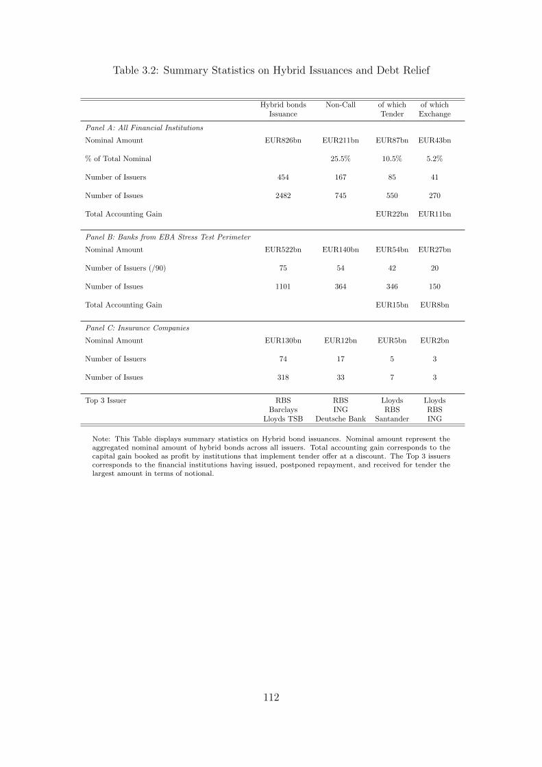
Table 3.2: Summary Statistics on Hybrid Issuances and Debt Relief

Hybrid bonds Non-Call of which of whichIssuance Tender Exchange

Panel A: All Financial Institutions

Nominal Amount EUR826bn EUR211bn EUR87bn EUR43bn

% of Total Nominal 25.5% 10.5% 5.2%

Number of Issuers 454 167 85 41

Number of Issues 2482 745 550 270

Total Accounting Gain EUR22bn EUR11bn

Panel B: Banks from EBA Stress Test Perimeter

Nominal Amount EUR522bn EUR140bn EUR54bn EUR27bn

Number of Issuers (/90) 75 54 42 20

Number of Issues 1101 364 346 150

Total Accounting Gain EUR15bn EUR8bn

Panel C: Insurance Companies

Nominal Amount EUR130bn EUR12bn EUR5bn EUR2bn

Number of Issuers 74 17 5 3

Number of Issues 318 33 7 3

Top 3 Issuer RBS RBS Lloyds LloydsBarclays ING RBS RBS

Lloyds TSB Deutsche Bank Santander ING

Note: This Table displays summary statistics on Hybrid bond issuances. Nominal amount represent theaggregated nominal amount of hybrid bonds across all issuers. Total accounting gain corresponds to thecapital gain booked as profit by institutions that implement tender o↵er at a discount. The Top 3 issuerscorresponds to the financial institutions having issued, postponed repayment, and received for tender thelargest amount in terms of notional.

112

Table 3.3: Contingent Debt Relief Users

Logit Non-Call User Logit Tender User

(A) (B) (C) (D) (E) (F)Tier 1 Ratio -0.143** -0.151** -0.314** -0.219

(-2.16) (-2.17) (-2.14) (-1.41)

RWA / Assets 408.791*** 1152.144**(2.85) (2.46)

Liabilities in Fair Value 1.039*** 0.820** -2.383** -3.077**(2.87) (2.34) (-2.02) (-1.97)

Log(Assets) 0.296** 0.240* 0.561*** 1.209*** 1.509*** 2.980***(2.28) (1.94) (4.58) (4.28) (4.51) (4.10)

Deposits / Total Debt 0.020 0.016 0.005 -0.010 -0.009 -0.053(1.63) (1.17) (0.37) ( -0.61) (-0.61) (-1.60)

Listed Dummy 0.055 0.086 -0.167 1.655* 2.515*** 3.678***(0.14) (0.21) (-0.46) (1.79) (3.08) (4.55)

Bank Type FE Yes Yes Yes Yes Yes YesCluster Country Country Country Country Country CountryPseudo R2 0.2090 0.2348 0.2519 0.4039 0.4662 0.5425N 179 179 171 162 162 154

Note: This Table presents logit regression coe�cients on the use of contingent debt reliefs. The left handsidevariable is a dummy variable equal to one if the financial institution has implemented at least one non-call on hybrid bonds over the period 2009-2011 for column (A) to (C), and equal to one if the financialinstitution has implemented at least one tender on hybrid bonds over the period 2009-2011 for column (D)to (E). Financial data is as per 2008. Liabilities in Fair Value is a dummy variable equal to one if the bankis using fair value accounting for its liabilities. Bank type is defined as per Bankscope. Standard errors areclustered at the country level. T-statistics are displayed below their coe�cient of interest.

113

Table 3.4: Predictions of Contingent Debt Relief Value E↵ects

RelaxingRegulatory Capital

Constraint

Negative SignalingE↵ect

ReducingRisk-ShiftingIncentives

Debt Value + - +

Equity Value + - -

Note: This Table presents the predictions on debt and equity value for the three hypotheses developed inSection 5.

114

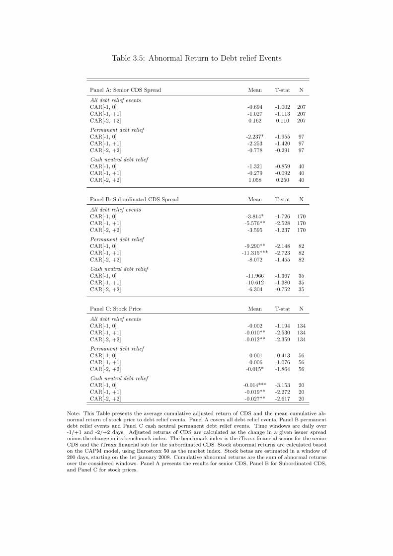
Table 3.5: Abnormal Return to Debt relief Events

Panel A: Senior CDS Spread Mean T-stat N

All debt relief eventsCAR[-1, 0] -0.694 -1.002 207CAR[-1, +1] -1.027 -1.113 207CAR[-2, +2] 0.162 0.110 207

Permanent debt reliefCAR[-1, 0] -2.237* -1.955 97CAR[-1, +1] -2.253 -1.420 97CAR[-2, +2] -0.778 -0.291 97

Cash neutral debt reliefCAR[-1, 0] -1.321 -0.859 40CAR[-1, +1] -0.279 -0.092 40CAR[-2, +2] 1.058 0.250 40

Panel B: Subordinated CDS Spread Mean T-stat N

All debt relief eventsCAR[-1, 0] -3.814* -1.726 170CAR[-1, +1] -5.576** -2.528 170CAR[-2, +2] -3.595 -1.237 170

Permanent debt reliefCAR[-1, 0] -9.290** -2.148 82CAR[-1, +1] -11.315*** -2.723 82CAR[-2, +2] -8.072 -1.455 82

Cash neutral debt reliefCAR[-1, 0] -11.966 -1.367 35CAR[-1, +1] -10.612 -1.380 35CAR[-2, +2] -6.304 -0.752 35

Panel C: Stock Price Mean T-stat N

All debt relief eventsCAR[-1, 0] -0.002 -1.194 134CAR[-1, +1] -0.010** -2.530 134CAR[-2, +2] -0.012** -2.359 134

Permanent debt reliefCAR[-1, 0] -0.001 -0.413 56CAR[-1, +1] -0.006 -1.076 56CAR[-2, +2] -0.015* -1.864 56

Cash neutral debt reliefCAR[-1, 0] -0.014*** -3.153 20CAR[-1, +1] -0.019** -2.272 20CAR[-2, +2] -0.027** -2.617 20

Note: This Table presents the average cumulative adjusted return of CDS and the mean cumulative ab-normal return of stock price to debt relief events. Panel A covers all debt relief events, Panel B permanentdebt relief events and Panel C cash neutral permanent debt relief events. Time windows are daily over-1/+1 and -2/+2 days. Adjusted returns of CDS are calculated as the change in a given issuer spreadminus the change in its benchmark index. The benchmark index is the iTraxx financial senior for the seniorCDS and the iTraxx financial sub for the subordinated CDS. Stock abnormal returns are calculated basedon the CAPM model, using Eurostoxx 50 as the market index. Stock betas are estimated in a window of200 days, starting on the 1st january 2008. Cumulative abnormal returns are the sum of abnormal returnsover the considered windows. Panel A presents the results for senior CDS, Panel B for Subordinated CDS,and Panel C for stock prices.

Table 3.6: Cross-section of CDS spread and Stock price reaction

CDS adjusted return Stock abnormal return

(A) (B) (C) (D) (E) (F)

Panel A: All Debt Relief Events

Tender O↵er -6.915* 0.001(-1.83) (0.17)

Cash Tender -6.843** -2.345 0.008 0.053***(-2.05) (-0.30) (1.22) (3.36)

Cash Tender * Leverage -0.245 -0.002***(-0.79) (-3.19)

Exchange O↵er -6.994 -31.515* -0.011* 0.016(-1.35) (-1.71) (-1.92) (0.83)

Exchange O↵er * Leverage 1.320* -0.001(1.68) (-1.08)

Leverage -0.396* -0.000(-1.87) (-0.60)

Log(Assets) 0.684 0.690 2.023 -0.003 -0.003 0.001(0.65) (0.66) (1.22) (-1.40) (-1.51) (0.53)

Quarter FE Yes Yes Yes Yes Yes YesCluster Issuer Issuer Issuer Issuer Issuer IssuerR2 0.1348 0.1348 0.1799 0.0887 0.133 0.2705N 373 373 351 137 137 118

Panel B: Exchange O↵ers Only

Exchange into Senior -15.031 -318.256* 0.008(-0.70) (-1.88) (0.75)

Exc. Senior * Leverage 14.849*(1.99)

Exchange into Equity -19.697* -57.741** 0.052***(-1.90) (-2.32) (3.71)

Exc. Equity * Leverage 2.203(1.67)

Log(Assets) 3.879* 0.305 -0.008(2.03) (0.15) (-1.58)

Leverage 0.132(0.92)

Quarter FE Yes Yes YesCluster Issuer Issuer IssuerR2 0.473 0.5186 0.7183N 91 89 26

Note: This table displays OLS regression coe�cients where the left hand side variable is CDS adjustedchange in columns (A) to (C), and stock price abnormal return in columns (D) to (E). Regressions (A) to(C) include controls for ranking and level of CDS spread. Tender O↵er, Cash Tender, Exchange O↵er aredummies variables indicating a debt relief of this type. Exchange into Senior and Exchange into Equityare dummy variables indicating an exchange o↵er into senior notes and equity, as opposed to an exchangeinto subordinated / hybrid debt. Leverage is defined as total assets over total regulatory capital. Standarderrors are clustered at the issuer level. T-statistics are displayed below their coe�cient of interest.

116

Table 3.7: Impact of Debt Relief on Economic Performance (ROA)

Hybrid User Non Call User Tender User

(A) (B) (C) (D) (E) (F)Post x Treated 0.838*** 0.551* 1.002** 0.736* 0.596* 0.352

(2.66) (1.66) (2.46) (1.68) (1.83) (0.95)

Post x Treated x Capital Gain 140.316** 114.121 114.406*(% Assets) (2.14) (1.28) (1.79)

Non-Call -0.633** -0.645** -0.772** -0.778** -0.548** -0.573**(-2.05) (-2.07) (-2.42) (-2.42) (-2.37) (-2.47)

Seasonal Equity O↵ering -0.192 -0.216 -0.153 -0.188 0.035 -0.010(-1.01) (-1.09) (-0.50) (-0.58) (0.22) (-0.05)

Change in Assets 1.807*** 1.807*** 1.730** 1.728** 0.369 0.373(3.11) (3.10) (2.05) (2.04) (1.34) (1.32)

Treated 0.025 0.033 0.071 0.087 -0.182 -0.166(0.15) (0.20) (0.32) (0.38) (-1.08) (-0.96)

Other Controls Yes Yes Yes Yes Yes YesYear FE Yes Yes Yes Yes Yes YesCluster Issuer Issuer Issuer Issuer Issuer IssuerR2 0.1478 0.1484 0.137 0.1375 0.3875 0.3949N 684 684 318 318 126 126

Note: This table displays OLS regression coe�cients where the left handside variable is Return On Assets(ROA) over the period 2007 - 2011. Treated is a dummy variable for having a debt relief in any year,post ⇥ treated a dummy variable for having a debt relief during this given year or a previous year, andpost⇥treated⇥CapitalGain the interaction term with the size of capital gain from the debt relief, expressedin % of total assets. I control for repayment postponement of hybrid bonds and seasonal equity o↵eringwith dummies for such events in a given year. Columns (A) to (D) present OLS regression analysis, whilecolumns (E) and (F) present an IV analysis, where post⇥ treated is the endogenous regressor. Regressionsinclude controls for previous accounting exercise total assets, Tier 1 capital ratio, client deposits over totalfunding, impaired loans over assets, risk weigthed assets over total assets, and yearly change in total assets,as well as a dummy variable for being publicly listed. Standard errors are clustered at the issuer level.T-statistics are displayed below their coe�cient of interest.

117

Table 3.8: The Lending Channel

OLS Hybrid User OLS Non Call User

Log(Loans) RWA/ Int. Income/ Log(Loans) RWA/ Int. Income/Assets Assets Assets Assets

(A) (B) (C) (D) (E) (F)Post x Treated 0.167* 0.001** 0.003** 0.181** 0.001*** 0.005***

(1.91) (2.16) (2.03) (2.62) (3.03) (2.75)

Non-Call -0.067 0.000 0.002 -0.110** 0.000 -0.002(-0.70) (0.82) (0.92) (-2.17) (-0.24) (-1.36)

Seasonal Equity O↵ering -0.170 0.000 -0.000 -0.036 0.000 0.002(-1.42) (0.65) (-0.23) (-0.29) (1.50) (1.04)

Change in Assets 1.491*** -0.000 0.003 0.994*** -0.001** 0.001(3.46) (-0.69) (0.92) (3.11) (-2.00) (0.28)

Treated -0.106 0.000 -0.001 -0.092 0.000 -0.002(-1.02) (0.09) (-0.50) (-0.79) (0.15) (-1.21)

Other Controls YES YES YES YES YES YESYear FE Yes Yes Yes Yes Yes YesCluster Issuer Issuer Issuer Issuer Issuer IssuerR2 0.7003 0.5003 0.1407 0.8004 0.5329 0.222N 710 678 710 329 316 330

Note: This table displays the coe�cients of OLS regression, where the left handside variable is indicatedin the column title. Non Op. Income / Assets means non operating income divided by total assets. OpIncome / Assets means operating income divided by total assets. Int. Income / Assets is for interest incomeover total assets, and RWA / Assets stands for Risk Weighted Assets over total assets. Standard errors areclustered at the issuer level. T-statistics are displayed below their coe�cient of interest.

118

Table 3.9: Robustness with Propensity Score Matching

Panel A: Economic Performance

ROA

(A) (B)Post x Treated 0.383* 0.153

(1.81) (0.66)

Post x Treated x Capital Gain 114.849**(2.35)

Non-Call -0.650** -0.660**(-2.08) (-2.11)

Seasonal Equity O↵ering -0.052 -0.084(-0.35) (-0.54)

Change in Assets 0.504 0.511(1.52) (1.52)

Treated 0.074 0.068(0.40) (0.37)

Other Controls Yes YesYear FE Yes YesCluster Issuer IssuerR2 0.2502 0.2569N 167 167

Panel B: Lending Channel

Log(Loans) RWA/ Int. Income/Assets Assets

(A) (B) (C)Post x Treated 0.142* 0.001* 0.001

(1.91) (1.73) (0.59)

Non-Call -0.157 -0.000 0.001(-1.07) (-0.24) (0.87)

Seasonal Equity O↵ering -0.091 0.000 -0.001(-0.91) (-0.18) (-0.96)

Change in Assets 0.588*** 0.000 -0.002(3.37) (0.21) (-1.09)

Treated 0.100 0.001 0.002(0.73) (1.45) (0.96)

Other Controls Yes Yes YesYear FE Yes Yes YesCluster Issuer Issuer IssuerR2 0.8617 0.5853 0.5157N 169 166 170

Note: This table displays the coe�cients of OLS regressions, where the left hand side variables are Returnon Assets (ROA), Log(Loans) and Risk Weighted Assets over Total Assets. Variables are as per Table 8 and9. The control group is constituted using a propensity score matching methodology on using a contingentdebt relief. The control group includes the five closest matches, with possible replacements. Standarderrors are clustered at the issuer level. T-statistics are displayed below their coe�cient of interest.

119

Table 3.10: Government Bail out e↵ects vs. Contingent Debt reliefs

Hybrid User Non Call User Tender User(A) (B) (C)

Post x Treated 0.702** 0.883** 0.563*(2.20) (2.14) (1.73)

Treated 0.481 0.621 -0.100(1.51) (1.60) (-0.51)

Post b x Treated b -0.806 -0.824 0.500(-0.75) (-0.61) (1.48)

Treated b -0.703** -1.171** -0.570**(-2.51) (-2.55) (-2.27)

Non Call -0.507* -0.726** -0.592**(-1.93) (-2.52) (-2.40)

Seasonal Equity O↵ering -0.195 -0.080 0.029(-1.08) (-0.31) (0.17)

Other Controls Yes Yes YesYear FE Yes Yes YesCluster Issuer Issuer IssuerR2 0.1828 0.201 0.4224N 684 318 126

Note: This table displays the coe�cients of OLS regressions, where the left handside variable is ReturnOn Assets (ROA) over the period 2007 - 2011. Treated is a dummy variable for having a debt relief inany year, post ⇥ treated a dummy variable for having a debt relief during this given year or a previousyear. Treated b is a dummy variable for having benefited from a government bail out in any year, andpost b⇥ treated b a dummy variable for having a debt relief during this given year or a previous year. Allother controls are the same as in Table 6, namely: previous accounting exercise total assets, Tier 1 capitalratio, client deposits over total funding, impaired loans over assets, risk weigthed assets over total assets,and yearly change in total assets, as well as a dummy variable for being publicly listed. Standard errorsare clustered at the issuer level. T-statistics are displayed below their coe�cient of interest.

120

Table 3.11: Country Group Trends

Hybrid User Non Call User Tender User(A) (B) (C)

Post x Treated 0.850** 0.986** 0.579*(2.57) (2.23) (1.73)

Non-Call -0.638** -0.817** -0.556**(-2.00) (-2.40) (-2.29)

Seasonal Equity O↵ering -0.263 -0.2767 -0.0883(-1.28) (-0.80) (-0.64)

Change in Assets 1.957*** 1.819** 0.546*(3.02) (2.01) (1.92)

Treated 0.065 0.228 -0.113(0.41) (1.07) (-0.60)

Scandinavia*Year FE Yes Yes YesPeriphery*Year FE Yes Yes YesRest of Europe Control Control ControlYear FE Yes Yes Yes

Other Controls Yes Yes YesCluster Issuer Issuer IssuerR2 0.1688 0.1599 0.4409N 684 318 126

Note: This table displays the coe�cients of OLS regressions with the same specification as Table 3.7.Regression also includes dummies variables for Eurozone periphery countries (Portugal, Italy, Ireland,Greece and Spain), as well as Scandinavian countries, interacted with year fixed e↵ects. Standard errorsare clustered at the issuer level. T-statistics are displayed below their coe�cient of interest.

121

Chapter 4

Conclusion

The three chapters of this dissertation studies the retail market for structured products,

the use of toxic loans by local governments, and the development of contingent capi-

tal instruments for financial institutions. This dissertation gives an overview of possible

motives for financial innovation: obfuscation, political agenda, or strengthening of bank

balance sheets. All three of these possible motives illustrate the ambivalence of financial

innovation. Innovative financial products can not only be a powerful tool for a sound

financial sector, but also an instrument of rent extraction from less sophisticated stake-

holders. This dual nature of financial innovation raises the question, among others, of

its regulation. Innovation and regulation often come hand in hand, but the question of

regulating financial innovation itself raises challenges di�cult to overcome, if only due to

the diversity of the fields in which it plays a role. Developing an approval process as for

the pharmaceutical industry, in the line of the proposition by Posner and Weyl (2013),

is consistent with the potential damage that innovative financial products can cause, but

seems di�cult to implement. To specialize a watchdog on financial innovation could also

be a promising road, but this option will need to be insulated from lobbying influences.

This dissertation is a first step towards better understanding financial innovation. The

next steps of my research agenda will lead me towards two other fields: education and

entrepreneurship. Income contingent loans, and crowdfunding are two promising forms

of financial innovation that deserve a thorough analysis.

122

Chapter 5

Appendices

123

Appendix A Chapter 1

Appendix A.1 Typology of Retail Structured Products

Product Underlying

Asset Name Description (in frequency order)

Equity (Single Index) Eurostoxx50, FTSE100, SP500, DAX, Ibex35, OMSX30, Nikkei225, CAC40, BRIC40Equity (Single Stock) Deutsche Bank, Credit Suisse, Daimler, Zurich Finance, Roche, Abb, BASF, UBS, Siemens,

Allianz, NestleCommodity Gold, brent, electricity, silver, cornForeign Exchange Euro/USD, PLN/Euro, CSK/Euro, CHF/EuroCredit Default The risk of default of a company or a countryInterest Rates Euribor, Libor, Swap rateOther Inflation, Funds

Main Feature (Primary Structure)

Structure Name Definition

Altiplano The product o↵ers a capital return of 100%, plus a series of fixed coupons on each sub periodsif the underlying is above a predefined barrier.

Floater The product o↵ers a capital return of 100% plus a series of coupons that rise when theunderlying reference rate rises.

Pure Income The product o↵ers a capital return of 100% plus a series of fixed coupons.Digital The product o↵ers a capital return of 100%, plus a fixed coupon paid at maturity if the

underlying is above a predefined barrier.Call The product o↵ers a capital return of 100% plus a fixed participation in the rise of the

underlying.Put The product o↵ers a capital return of 100% plus a fixed participation in the absolute value

of the fall of the underlying.Spread The product o↵ers a capital return of 100% plus a participation related to the spread between

the performances of di↵erent underlyings (shares, rates.).Bull Bear The final return is based on a percentage of the absolute performance of the underlying at

maturity.

Feature Type 1: Initial Subsidy (facultative)

Feature Name Definition

DiscountGuaranteed RateBonus

Feature Type 2: Underlying Selection (facultative)

Feature Name Definition

Best of Option The return is based on the performance of the best performing underlying assets.Worst of Option The return is based on the participation in the performance of the worst performing under-

lying assets.Himalaya A pre-selected number of best-performing assets are permanently removed from the basket,

or frozen at their performance level, at the end of each period until the end of the investment.Kilimanjaro The lowest performing assets as well as the best performing assets have been progressively

eliminated, or ignored from subsequent calculations, during the investment period.Rainbow Best performing assets are weighted more heavily than those which perform less well.

Feature Type 3: Exposure Modulation, Increased Downside (facultative)

Feature Name Definition

Reverse Convertible The product is capital guaranteed unless a performance criterion is not satisfied. In this case,the capital return is reduced by the percentage fall in the underlying, or the product paysback a predefined number of shares/bonds.

Precipice The product is capital guaranteed unless a performance criterion is not satisfied.

124

Feature Type 4: Exposure Modulation, Limited Upside (facultative)

Feature Name Definition

Cap The return is based on the participation in the performance of the worst performing under-lying assets.

Fixed Upside The best performances of a basket of stocks or of a set of subperiod returns are replaced bya predetermined fixed return.

Flip Flop The coupons are fixed in the first periods, and the distributor has the right to switch youinto floating.

Feature Type 5: Path Dependence (facultative)

Feature Name Definition

Cliquet The final return is determined by the sum of returns over some pre-set periods.Asian Option The final return is determined by the average underlying returns over some pre-set periods.Parisian Option The value of the return depends on the number of days in the period in which the conditions

are satisfied.Averaging The final index level is calculated as the average of the last readings over a given period

(more than one month).Delay Coupons are rolled up and paid only at maturity.Catch-up If a coupon is not attributed in a given period because the condition required for the payment

is not met, then that missed coupon and any subsequently missed coupon will be rolled-upand attributed the next period when the condition is met.

Lookback The initial/final index level is replaced by the lowest/highest level over the period.

Feature Type 6: Exotic Condition (facultative)

Feature Name Definition

American Option The conditions must be satisfied during the whole considered period.Range The performance of the underlying is within a range.Target The sum of the coupon reaches a predefined level.Moving Strike The conditional levels are moving.Bunch The top barrier/cap concerns each asset whereas the bottom barrier concerns the whole

basket.Podium The underlying is a basket and the final returns depend on the number of shares satisfying

the conditions.Annapurna The condition must be satisfied for any security in the underlying basket.

Feature Type 7: Early Redemption (facultative)

Feature Name Definition

Knockout The product matures early if specific conditions are satisfied.Callable The issuer can terminate the product on any coupon date.Puttable The investor can terminate the product on any coupon date.

This table describes how a pay-o↵ formula is broken down into distinct features. Each family of facultativefeatures contains features that are mutually exclusive. A structured product possesses exactly one mainfeature, which defines the primary structure of the product.

125

Appendix A.2 - Figures

Figure A.0: . Average Product Complexity by Year

This figure shows the average of our robustness checks proxies for complexity by year. Number ofScenarios measures the number of conditions embedded in the final payo↵ formula, and DescriptionLength the number of characters in the standardized text description of the payo↵ formula.

126

Appendix A.3 - Tables

Table A.1: . The 20 Main Distributors in terms of Market Share in 2010

Name Country Market N. of Type Distribution Countriesof Origin Share in % Payo↵s

Deutsche Volks & Rai↵eisenb. DE 11.6 2.8 Savings B AT DE IT PL

Deutsche Sparkassen DE 10.6 2.7 Savings B AT CZ DE

Deutsche Bank DE 4.8 3.2 Commercial B AT BE DE IT NLPL PT ES UK

UBS CH 4.1 2.3 Private B AT BE FR DE ITNL NO ES

RBS UK 3.9 2.1 Commercial B AT BE DK FI FR DE IEIT NL PT ES SE UK

KBC BE 2.8 2.8 Commercial B BE CZ FR HU IE NL PLUK

Santander ES 2.7 2.4 Commercial B PL PT ES UK

Unicredit IT 2.7 2.7 Commercial B AT CZ DE HU IT PL ES

Commerzbank DE 2.5 2.8 Commercial B AT BE FR DE HUIT NL NO PL ES

Barclays UK 2.5 2.5 Commercial B AT BE CZ FR DE IEIT NL PT ES UK

Bnp Paribas FR 2.4 3.1 Commercial B AT BE FR DE HU ITNL PL PT ES UK

Nordea SE 2.3 2.0 Commercial B DK FI IT NO PL SE

Garantum FI 2.1 3.5 Private B FI SE

Societe Generale FR 2.1 3.2 Commercial B AT BE CZ FR DEIT NL PL ES UK

Caja De Ahorros ES 2.0 2.1 Savings B PT ES

Investec ZA 1.9 2.5 Private B IE UK

Seb SE 1.4 2.1 Commercial B DK FI DE NO PL SE

Osterreichische Volksbanken AU 1.4 1.5 Commercial B AT DE HU

ING NL 1.4 2.7 Commercial B AT BE CZ FR DE IT NLPL ES UK

Jp Morgan US 1.1 3.2 Private B AT BE FR DE IT NL PLES UK

Market shares are computed in terms of number of product issued in Europe in 2010. Countries of distri-bution are idicated with their ISO 3166 code

127

Tab

leA.2:.Detailsof

theretailstructuredproduct

issued

inJu

ly2009

(1/4)

Pro

duct

Name

Pro

vider

Name

Country

Cre

dit

Matu

rity

Number

Marku

pEntryfees

Man

a.fees

Risk

inyears

Payo↵

sin

%in

%in

%

Sprint

Zertifikat

Hyp

overeinsban

kGerman

yyes

4.4

1-8.0

2.0

0.0

Summer

Invest

AllianzBelgium

Belgium

no

4.9

1-4.6

4.0

0.0

Phoenix

2Ban

kof

Scotlan

dIrelan

dno

3.9

2-3.6

3.5

0.0

EuropaAnleihe10%

PlusIi08

/09-08/14

Barclays

Austria

yes

52

-3.6

5.0

0.0

EuropaAnleihe10%

Plus07/09-07/14

Barclay

sAustria

yes

52

-3.5

5.0

0.0

Eurostoxx50

ZinsAnleihe4

Barclays

Austria

yes

52

-2.9

2.5

0.0

4YEurMarketRecoveryNote

ING

Belgium

yes

41

-2.4

0.0

0.0

EurozoneCou

pon

Note

IngBan

kNetherlands

yes

52

-2.0

0.0

0.0

DzBan

kVrGaran

tieanleihe09/14

DzBan

kGerman

yyes

52

-1.9

2.0

0.0

3YMarketRecoveryNote

ING

Belgium

yes

31

-1.7

0.0

0.0

EuropaKupon

Anleihe

Lan

desban

kBerlin

German

yyes

51

-1.4

0.0

0.0

Seguro

Rentabilidad

Eurostoxx114Db

DeutscheBan

kSpain

no

3.4

2-1.1

0.0

1.4

Barrier

NoteDjEurostoxx5

0IN

GBelgium

yes

1.5

2-1.1

0.0

0.0

Seguro

Rentabilidad

Eurostoxx119Db

DeutscheBan

kSpain

no

3.9

2-1.1

0.0

1.4

CsGaran

t100Anleihe13

DjEuro

Stoxx

50CreditSuisse

Austria

yes

52

-1.1

2.0

0.0

EuropaProtect-A

nleihe07/09

WestLb

German

yyes

43

-1.1

2.0

0.0

Seguro

Rentabilidad

Eurostoxx122Db

DeutscheBan

kSpain

no

4.4

2-0.9

0.0

1.2

Euro

Boo

ster

200%

SwissLifeBan

quePrivee

France

yes

54

-0.9

0.0

0.0

Europa-Anleihe

Lan

desban

kBerlin

German

yyes

52

-0.8

0.0

0.0

Seguro

Rentabilidad

Eurostoxx110Db

DeutscheBan

kSpain

no

2.9

2-0.7

0.0

1.0

CsTop

Bon

us115200

Credit

Suisse

Austria

yes

52

-0.7

3.5

0.0

Partizipationsanleihe01/09

Nordlb

German

yyes

42

-0.4

0.0

0.0

Cp100Cap

-Perform

ancean

leihe

Sal.Oppenheim

Austria

yes

42

-0.4

1.5

0.0

Vital

Ibex

Bolsa

Garan

tizado

Caja

Vital

Kutxa

Spain

no

2.5

2-0.3

5.0

5.6

Lbbw

Safe-AnleiheMitCap

Lan

desban

kBw

German

yyes

42

-0.3

1.0

0.0

128

Tab

leA.3:.Detailsof

theretailstructuredproduct

issued

inJu

ly2009

(2/4)

Pro

duct

Name

Pro

vider

Name

Country

Cre

dit

Matu

rity

Number

Marku

pEntryfees

Man

a.fees

Risk

inyears

Payo↵

sin

%in

%in

%

IgcDjEurostoxx5

0-Ju

li2009

Van

Lan

schot

Ban

kiers

Netherlands

no

52

-0.1

2.0

3.3

Europa-Anleihe

Lan

desban

kBerlin

German

yyes

52

-0.0

2.0

0.0

DjEurostoxx5

0Partizipations-Anleihe

Lan

desban

kBerlin

German

yyes

53

0.2

1.5

0.0

Objectif7.5%

Juin

2009

SwissLifeBan

quePrivee

France

yes

84

0.3

0.0

0.0

EasyBon

us-Zertifikat

WestLb

German

yyes

4.3

20.3

1.0

0.0

Equ

ityProtectionSwitchab

leDeutscheBan

kItaly

yes

52

0.5

3.3

0.0

Objectif7,5%

Distribution

Juillet2009

SwissLifeBan

quePrivee

France

yes

84

0.6

0.0

0.0

BsGaran

tiaExtra

10Ban

coSab

adell

Spain

no

3.1

30.8

5.0

3.0

EuropaProtect-A

nleiheExtra

03/09

WestLb

German

yyes

62

0.8

2.5

0.0

VrExtrachan

ceIi

DzBan

kGerman

yyes

4.4

21.0

3.0

0.0

Bbv

aOportunidad

EuropaBp

Bbv

aSpain

no

2.9

21.1

5.0

6.8

Euro

Boo

ster

SwissLifeBan

quePrivee

France

yes

54

1.2

0.0

0.0

Ten

Pea

Barclays

France

no

16

1.2

2.0

3.0

DzBan

kBon

uschan

ceCon

trol

309/13

DzBan

kGerman

yyes

3.5

21.4

0.0

0.0

DzBan

kBon

uschan

ceCon

trol

Iii09/13

DzBan

kAustria

yes

3.5

21.4

0.0

0.0

Athena11%

Airbag

SwissLifeBan

quePrivee

France

yes

84

1.4

0.0

0.0

Bon

usPro

Zertifikat

Hyp

overeinsban

kGerman

yyes

4.4

11.5

2.0

0.0

Best-Entry

Garan

tV-A

nleihe

BayerischeLan

desban

kGerman

yyes

4.5

21.6

1.0

0.0

EuropaProtect

AnleihePlus

JpmorganChase

German

yyes

62

1.6

2.0

0.0

Bbv

aEuropaGaran

tizado

Bbv

aSpain

no

2.9

31.7

5.0

3.6

Kbc-LifeMiSecurity

Europe2

KbcVerzekeringen/CbcAssurance

Belgium

no

7.6

21.8

3.0

18.2

Callable

Boo

ster

Notes

Barclay

sBelgium

yes

63

1.9

0.0

0.0

EurostoxxSerenite2009

CreditSuisse

France

no

62

2.0

3.0

12.0

Dep

ositoIm

batible

8-5

Bbk

Spain

no

3.4

42.1

0.0

0.0

Rentenb

ankCap

ped

Cap

ital

Protected

Note

AbnAmro

Ban

kNetherlands

yes

72

2.1

0.0

0.0

129

Tab

leA.4:.Detailsof

theretailstructuredproduct

issued

inJu

ly2009

(3/4)

Pro

duct

Name

Pro

vider

Name

Country

Cre

dit

Matu

rity

Number

Marku

pEntryfees

Man

a.fees

Risk

inyears

Payo↵

sin

%in

%in

%

DzBan

kIndexklassikGaran

t509/13

DzBan

kGerman

yyes

4.4

22.1

2.5

0.0

DzBan

kIndexklassikGaran

tV

09/13

DzBan

kAustria

yes

4.4

22.1

2.5

0.0

DjEurostoxx50

Bon

usMinim

axLan

desban

kBerlin

German

yyes

33

2.4

0.5

0.0

Exp

ress

Zertifikat

DeutscheBan

kAustria

yes

24

2.4

1.0

0.0

Mes-R

endem

ents

10%

Finan

ceSelection

France

yes

55

2.6

0.0

0.0

EuropaCallable

Protect

Anleihe

JpmorganChase

German

yyes

54

2.6

1.5

0.0

CsMem

oryExp

ress

Zertifikat6

CreditSuisse

German

yyes

65

2.6

2.5

0.0

Autofocus9%

CreditMutuel

Arkea

France

no

53

2.6

2.0

3.5

EuropaGaran

tPlus-Anleihe

Lan

desban

kBerlin

German

yyes

62

2.7

1.0

3.0

Btv

EuropaBon

usGaran

tieanleihePlusIii2009

-2014/12

Btv

Ban

kAustria

yes

5.5

42.7

0.0

0.0

Dexia

Clickinvest

BIndex

Linked7

Dexia

Ban

kBelgium

no

5.1

22.8

2.5

11.9

CsTop

Bon

usChan

ce3

CreditSuisse

German

yyes

4.4

22.8

1.5

0.0

Eurostoxx50

Flex-Exp

ress

02/09

WestLb

German

yyes

31

3.0

1.0

0.0

CsTop

Mem

oryExp

ress

Credit

Suisse

German

yyes

46

3.1

1.0

0.0

Switch

ToBon

dNote

Fortis

Belgium

yes

54

3.1

0.0

0.0

Indexan

leihe

Nordlb

German

yyes

12

3.1

0.0

0.0

Dexia

Clickinvest

BIndex

Linked8

Dexia

Ban

kBelgium

no

5.1

23.3

2.5

11.9

Unigaran

t:Europa(2015)

UnionInvestment

German

yno

5.9

23.3

4.0

6.0

KbcClickplusEuropeBestOf42

KbcBan

kBelgium

no

8.6

33.8

2.5

19.1

CenteaFundClick

EuropeSurplus10

Centea

Belgium

no

8.6

33.8

2.5

17.0

Zan

onia-D

eep-Zertifikat

Lan

desban

kBw

German

yyes

43

3.8

1.0

0.0

Buon

oFruttiferoPostale

16D

Ban

coposta

Italy

yes

52

3.9

0.0

0.0

EurostoxxFast7%

SwissLifeBan

quePrivee

France

yes

84

4.0

0.0

0.0

DzBan

kExtrachan

cePro

V09/13

DzBan

kAustria

yes

42

4.3

2.3

0.0

DzBan

kExtrachan

cePro

509/13

DzBan

kGerman

yyes

42

4.3

2.3

0.0

130

Tab

leA.5:.Detailsof

theretailstructuredproduct

issued

inJu

ly2009

(4/4)

Pro

duct

Name

Pro

vider

Name

Country

Cre

dit

Matu

rity

Number

Marku

pEntryfees

Man

a.fees

Risk

inyears

Payo↵

sin

%in

%in

%

DzBan

kVrExtrachan

ceIii09/13

DzBan

kGerman

yyes

42

4.3

2.3

0.0

Exp

ress

Zertifikat

Hyp

overeinsban

kGerman

yyes

24

4.4

0.5

0.0

Bon

oAutocancelable

8%Cupon

Citi

Spain

yes

53

4.4

3.0

0.0

Wgz

Garan

t-Zertifikat22

Wgz

Ban

kGerman

yyes

62

4.5

2.0

0.0

Emtn

Mem

oryExp

ress-Zertifikat4

Societe

Generale

German

yyes

65

4.7

2.0

0.0

Bon

usCon

trol

IvDzBan

kAustria

yes

42

4.8

2.5

0.0

Seguro

RecuperacionEurostox

xDb

DeutscheBan

kSpain

no

31

5.3

0.0

1.0

Ban

kinter

Eurostox

x2012

Garan

tizado

Ban

kinter

Spain

no

33

5.4

5.0

6.8

Euro

Mem

ory

Nortia

France

yes

85

5.5

0.0

0.0

Reference

8,5%

Adequity

France

no

84

5.5

4.5

2.0

Optimiz

7%Societe

Generale

Italy

yes

8.2

25.6

0.0

0.0

StepDjEurostoxx50

Ban

caAletti

Italy

yes

33

5.8

0.0

0.0

Phoenix

Mem

ory

Adequity

Belgium

yes

45

5.8

0.0

0.0

Zan

onia-P

lus-Zertifikat

Lan

desban

kBw

German

yyes

44

6.0

1.0

0.0

Wgz

Airbag-ZertifikatMitCap

Wgz

Ban

kGerman

yyes

54

6.6

2.0

0.0

Wgz

Easyexp

ress-Zertifikat12

Wgz

Ban

kGerman

yyes

42

6.6

2.0

0.0

Buon

oFruttiferoPostale

P22

Ban

coposta

Italy

yes

52

7.2

0.0

0.0

FortisB

Fix

2009

BestOfClick

6BnpParibas

Fortis

Belgium

no

8.5

37.9

2.5

0.0

Elixis2

CreditAgricole

France

no

4.2

48.1

2.0

10.0

Cap

Garan

ti2015

CreditMutuel

France

no

5.9

28.1

3.0

2.5

Sevea

Gestion

PriveeIndosuez

France

no

54

8.8

2.5

12.5

Ing(L

)SelectisEuro

Equ

ity1

IngLuxembou

rgBelgium

no

4.5

39.2

3.0

6.8

BifCerti+

200

Alternea

Belgium

no

63

9.4

5.0

7.2

Orian

ceEpargn

e2

Credit

Agricole

France

no

6.8

211.8

0.0

0.0

Euro

Cap

2017

(EUro

Cap

2017)

HsbcAssurancesVie

France

no

63

11.9

0.0

0.0

RecoveryNote

AbnAmro

Ban

kNetherlands

yes

53

14.8

0.0

0.0

131

Appendix A.4 - Theoretical Framework (Model)

We develop a model in which firms strategically use financial complexity to mitigate competition. The

model is inspired by Carlin (2009), but di↵ers in that consumers are heterogeneously distributed across

firms and may face switching costs. For tractability purposes, the fraction of uninformed consumers is

taken as exogenous.

Model Setup

Consumers

Consider a market in which n firms produce a homogeneous retail financial product. In this market,

there is a unit mass of consumers M who each has a unit demand for the retail good. Each consumer i

maximizes the same utility function

Ui

= v � pi

where v is the fundamental value of the product and pi

its price.

Firms

Firms in this market face the same marginal production cost, which is fixed at zero, but di↵er in the

structure and level of the price that they charge. They can sell the financial product either in a simple

price structure, thereafter the ”package”, or in a complex one, implying no additive cost. In the complex

price structure, the price of the product is not observable by consumers.

Firms also di↵er in the fraction of consumers in their neighbor. A firm of rank j captures a fraction

↵j

of consumers, with 0 ↵j

1, ↵j+1 < ↵

j

andP

n

1 ↵j

= 1.

To simplify the analysis, we restrict the firms to choose prices in the interval [p;P ], with p > 0 and

P = v is the monopoly price.

Financial Sophistication

Consumers are divided into two groups: a fraction µ is uninformed, and a fraction 1 � µ is expert.

Expert consumers are knowledgeable about the price structure of a product and face no switching cost.

They consequently only buy simple products, whose prices they can observe, at the lowest price available.

In contrast, uninformed consumers are uneducated about prices even for a simple package, and face a

switching cost c > 0. As a result, uninformed consumers purchase the retail financial product from the

firm they are already on relationship with, independently of the price package.

Timing

The game is in two periods. In stage one, firms simultaneously set prices and decide if the price

structure is going to be complex or simple. In stage two, consumers buy the product with a strategy

based on their type.

Results

Consider the price of a simple product. There is free entry of firms. New entrants capture a fraction

↵ = 0 of consumers. Free entry implies that the price of a simply structured product is the minimum

price, p. If a firm j decides to sell the product with the simple price structure, it receives a fraction 1/ns

of the demand from experts - ns

denoting the number of firms with the same strategy - plus the demand

132

from the fraction ↵j

of captured uninformed consumers. Its profit is

⇧j,s

= p� µ

ns

+ ↵j

(1� µ)�

Consider now the price of a complex product. By selling the product in the complex package, a firm will

receive demand only from uninformed consumers who do not observe prices. It is optimal in this case to

sell the product at a maximum price P . The payo↵ of a firm selling the complex product is

⇧j,c

= ↵j

(1� µ)P

Firm j sells the product in a complex package if and only if

⇧j,c

� ⇧j,s

, ↵j

(1� µ)P � p� µ

ns

+ ↵j

(1� µ)�

, ↵j

� pµ

P (1� p)(1� µ)⇤ 1

ns

, ↵j

� A

ns

with A = pµ

P (1�p)(1�µ) This leads to the following proposition

Proposition 1 The tendency of a firm to sell a complex product increases with the share of uninformed

consumers it is initially in a relationship with.

We make the following assumption

Assumption 1

↵1 >A

n

Assumption 1 implies that it is optimal for the firm of rank 1, namely the one with the biggest

market share, to sell the product in the complex package if all other firms in the market choose to sell

the simple product.

Lemma 1 There exists a unique k such that:

• Firms of rank j, with 1 j k, choose to sell the product in the complex package

• Firms of rank j, with k < j n, choose to sell the product in the simple package

Proof.

Let denote f the function defined by:

f(k) = ↵k

� A

n� k + 1

By definition, ↵k

is a decreasing function of k, and � A

n�k+1 is also decreasing in k. In addition, Assump-

tion 1 implies that f(1) > 0 and f(n) < 0. Therefore, there exists a unique k such that for any j � k we

have f(j) � 0 whereas for any j < k we have f(j) 0.

133

Let �(n) define the fraction of complex products as a function of the number of competitors. We

have

�(n) =k

n

Now we make the assumption that we are in a neck-and-neck market, in which the distance between

two firms, measured by the di↵erence in market share ↵, is small. It implies

Assumption 2

↵k

� ↵k+1 <

A

n� k� A

n� k + 1

We obtain the following proposition

Proposition 2 In a neck-and-neck market, as competition increases, the fraction of complex products

increases as well (� increases).

Proof. By assumption, for any new entrant n+ 1 we have ↵n+1 = 0. We also have

8>>>>><

>>>>>:

↵k

� A

n� k + 1

↵k+1 <

A

n� k

↵k+1 < ↵

k

Since the market is neck-and-neck we have also

↵k

� ↵k+1 <

A

n� k� A

n� k + 1

implyingA

n� k + 1< ↵

k+1 <A

n� k< ↵

k

A new entrant will make the firm k+1 change its strategy and switch to a complex package. The fraction

of complex products increases

�(n+ 1) =k + 1

n+ 1

134

Appendix B Chapter 2

Appendix B.1 Types of Structured Debt Products and Risk

Classification

Products are presented by increasing level of risk according to the Gissler classification

(from ”Charte de bonne conduite entre les etablissements bancaires et les collectivites

locales”). For each type of products, summary statistics are provided in Table A2.

Barriers on Domestic Rate (Underlying Risk Level: 1)

These products lower cost of funding as long as the underlying index is above/under a

predefined barrier. Subsidy comes from the premium of the options sold, which could be

interest rate caps or floors. An example is the implicit sale of a floor:

coupon(t) =

8<

:US Libor(t)� x bps if US Libor(t) > 3%

3% otherwise.

The underlying index is a very liquid interest rate. Coupon structure does not include

any leverage e↵ect. Both the subsidy o↵ered to client and the bank margin are low

(<0.50% of notional). Barriers were the first products to enter the market in the late

1990s. Their coupon formula can be broken down into its vanilla loan component and an

embedded short put option:

V anilla loan coupon : US Libor(t)

Sale of a put

with a 3% strike :

8<

:� x bps if US Libor(t) > 3%

3% � US Libor(t) otherwise.

Inflation Products (Underlying Risk Level: 2):

This type of products is usually based on a barrier, or on an inflation spread. They often

include leverage to provide with su�cient subsidy, as inflation volatility is very low. A

standard payo↵ is:

Coupon(t) = Midswap(t) � 50 bps + 2 ⇥ Max(French Inflation(t) � Euro Inflation(t), 0%).

This illustrates the client’s view that the French inflation rate should remain below

the European inflation rate, which could be caused by entrance of new EU members from

135

Eastern Europe with historically higher inflation.

Steepeners (Underlying Risk Level: 3):

In a Steepener structure, the coupon is indexed to the Constant Maturity Swap (hereafter

CMS) curve slope and decreases the cost of funding when the slope of the curve is steep;

but increases the cost when the curve is flat or inverted. The CMS curve is built with the

equivalent fixed rates obtained when swapping Libor for all possible maturities. They

are based on di↵erent measures of the slope: [20-year swap rate - two-year swap rate],

[30-year swap rate - one-year swap rate], and in most cases [10-year swap rate - two-year

swap rate]. An example of payo↵ is:

Coupon(t) = 7%� 5⇥ (CMS 10Y (t)� CMS 2Y (t)).

Entering into a Steepener transaction represents a bet against the realization of for-

ward levels, which typically anticipate a flattening of the swap curve. The risk profile

of these products is higher than the one of Barrier products. This is mainly due to the

introduction of leverage in the coupon formula, usually without any cap.

Quantos (Underlying Risk Level: 4):

They represent variable interest rate products that are indexed on a foreign interest rate

with an a�ne formula. They exploit low spot rates and higher forward levels. Risk is

moderate as leverage is generally low and the underlying foreign interest rate has low

volatility. They are mainly structured on indices from countries with low interest rates,

such as Japan or Switzerland. A standard Quanto payo↵ is:

Coupon(t) = 2⇥ JPY Libor(t) or Coupon(t) = 1.5⇥ CHF Libor(t) + 1%.

FX Products (Underlying Risk Level: Out of Scale):

FX products are also based on an implicit sale of options. However FX options premiums

are much higher due to the high volatility of foreign exchange rates and remain high even

when strike levels are far from spot prices. This comes from the absence of mean-reversion

of foreign exchange rates in banks’ pricing models. This feature allows to structure

products with seemingly unreachable strikes, especially when historical levels bias the

client’s view. An example of payo↵ for an FX product is:

Coupon(t) = 3% + 50%⇥Max(1.44� EURCHF (t), 0%).

These products o↵er very strong coupon subsidy, especially on long maturity loans

136

when they bear no caps. One example is the 0% coupon loan by Depfa with Ville de Saint

Etienne on a 32-year maturity loan. The coupon is set at 0% for 9 years and remains at

this level afterwards as long as EURCHF is above EURUSD.

Cumulative Structures: (Underlying Risk Level: 1; Structure Risk Level: Out

of Scale)

Cumulative structures can be structured on any underlying: domestic/foreign interest

rates, FX rates, or inflation rates. They are based on an iterating coupon formula.

Coupon degradations therefore add up to each other. The formula often includes a

click feature that makes all degradations permanent; hence their nickname: snow balls.

Cumulative instrument structuring is based on selling a portfolio of forward-start options.

A typical coupon profile is:

Coupon(t) = Coupon(t� 1) + 2⇥Max(USD Libor 12M(t)� 6%, 0%).

Due to the iterating definition of the coupon, frequency of coupon payment is key

for the risk profile of the product. For a given leverage level, a quarterly cumulative

structure is four times more aggressive than an annual one. These products have been

dramatically impacted by the increase in volatility during the financial crisis, as they

bear no cap. They are usually more sensitive to volatility than to market direction (i.e.,

vega dominates delta).

137

Appendix B.2 Tables

Table B.6: Hedging

Pooled Regression Individual Regressions

Coe�cient St. Err. P-value Mean Coe↵. St. Dev. Co-e↵.

% Coe↵ > 0at 10% sig-nif.

% coe↵<0 at10% signif.

Euribor 3m -0.0162 0.0168 0.436 0.0122 0.047 3.98% 0.00%

CMS 10y - CMS 2y -0.0601 0.0504 0.355 -0.0193 0.0404 13.72% 1.33%

EURCHF -0.112 0.0963 0.364 0.237 0.3277 15.49% 3.54%

EURUSD 0.1681 0.1577 0.398 0.0982 0.2713 3.98% 0.00%

Note: This table contains summary statistics on regression coe�cients between the annual percentagechange in revenues and the percentage change in several financial indices. The pooled regression is runon the four indices, controlling for inflation and with local authorities type fixed e↵ects. Standard errorsof coe�cients are clustered by type of local authorities. Individual regressions are conducted for eachlocal government on each individual index, also controlling for inflation. Euribor 3m is the 3-month Eurointerbank o↵ered rate and CMS stands for Constant Maturity Swap and corresponds to the fixed rateobtained by swapping a Euribor coupon. For CMS 10y - CMS 2y, we use the first di↵erence. The sampleincludes all French regions, departments, as well as the 100 largest cities (226 French local authorities intotal) for which we have revenue data between 1999 and 2010. Index data are from Datastream and localauthorities’ revenues are from the French Finance Ministry.

138

Table B.7: Structured-Debt Breakdown

Notional Notional / Local Gov. Total Debt

All Regions Counties Intercities Cities All Regions Counties Intercities Cities

Aggregate 10429.9 1128.5 4801.9 1334.7 3164.91. BarriersAggregate 4970.7 532.3 1959.8 746.8 1731.8Share in % 47.70% 47.20% 40.80% 56.00% 54.70%Mean 17 21.3 20.4 9.8 18 10.20% 6.50% 8.80% 9.90% 12.70%Stdev 33.3 29.2 33.3 24 39.7 14.10% 8.70% 11.90% 17.20% 14.60%Max 342 99.2 161.7 167.9 342 95.50% 33.30% 67.90% 95.50% 69.90%% of use 57.70% 56.00% 60.40% 44.70% 65.60%2. SteepenersAggregate 2794.8 301.1 1417.5 329.4 746.7Share in % 26.80% 26.70% 29.50% 24.70% 23.60%Mean 9.5 12 14.8 4.3 7.8 5.20% 3.50% 5.80% 4.90% 5.30%Stdev 25.4 33.8 33.5 10.1 21 9.70% 11.20% 8.80% 9.30% 10.50%Max 275.8 162.4 275.8 54.4 151.4 70.50% 54.10% 41.60% 44.70% 70.50%% of use 39.90% 32.00% 51.00% 31.50% 37.50%3. FXAggregate 1543.9 87.2 968.3 152.5 335.8Share in % 14.80% 7.70% 20.20% 11.40% 10.60%Mean 5.3 3.5 10.1 2 3.5 2.10% 1.10% 2.50% 2.50% 1.80%Stdev 24.1 11.4 38.4 7.2 14.2 7.40% 3.80% 7.70% 9.40% 6.20%Max 240.8 52.9 240.8 47.4 112.6 66.70% 17.60% 44.00% 66.70% 36.80%% of use 14.00% 12.00% 18.80% 13.20% 10.40%4. InflationAggregate 357.8 102.3 120.2 30.7 104.5Share in % 3.40% 9.10% 2.50% 2.30% 3.30%Mean 1.2 4.1 1.3 0.4 1.1 0.60% 1.40% 0.40% 0.30% 0.70%Stdev 6.6 12.4 7 2.1 6.4 3.50% 5.50% 1.70% 1.50% 4.90%Max 64.4 49 64.4 12.9 60 46.10% 27.00% 11.90% 8.70% 46.10%% of use 7.20% 16.00% 8.30% 3.90% 6.30%5. QuantosAggregate 249.4 33.5 89.4 28.6 98Share in % 2.40% 3.00% 1.90% 2.10% 3.10%Mean 0.9 1.3 0.9 0.4 1 0.50% 0.40% 0.40% 0.30% 0.80%Stdev 3.5 4.2 3.4 2.4 4 1.90% 1.20% 1.30% 1.20% 2.70%Max 33.2 15.8 25.6 20.7 33.2 16.40% 1.20% 8.10% 7.80% 16.40%% of use 12.30% 12.00% 12.50% 6.60% 16.70%6. CumulativeAggregate 33.4 13 7.4 0 13Share in % 0.30% 1.20% 0.20% 0.00% 0.40%Mean 0.1 0.5 0.1 0 0.1 0.00% 0.10% 0.00% 0.00% 0.00%Stdev 1 2.6 0.8 0 0.8 0.30% 0.40% 0.30% 0.00% 0.30%Max 13 13 7.4 0 7.1 3.20% 2.00% 3.20% 0.00% 1.90%% of use 1.70% 4.00% 1.00% 0.00% 3.10%7. OthersAggregate 300.9 30 143.6 28.9 98.5Share in % 2.90% 2.70% 3.00% 2.20% 3.10%Mean 1 1.2 1.5 0.4 1 0.80% 0.30% 1.00% 0.50% 1.00%Stdev 4 4.4 4.6 2 4.5 3.70% 1.00% 3.70% 2.90% 4.50%Max 35.8 20 23.6 12.9 35.8 36.10% 3.40% 27.90% 22.10% 36.10%% of use 8.50% 8.00% 11.50% 3.90% 9.40%

Note: This table contains summary statistics on the di↵erent types of structured debt for a sample ofFrench local governments. The data are obtained from a survey conducted by a specialized consulting firmas of December 31, 2007 (Dataset A). The left panel of this table displays statistics on aggregated and localgovernment-level amounts of debt. Figures are in millions of euros, except for share in % and % of use.Aggregate denotes the sum of the debt notional amount over all local governments. Share in % representsaggregated amount of a given debt instrument in the sample divided by aggregated total structured debt ofthe sample. The right panel displays statistics on the relative breakdown by debt instruments at the localgovernment level. For instance, a local government whose debt consists in EUR70m of vanilla bank loansand EUR30m of FX linked debt will be considered as a local government with 30% of FX linked debt.

139

Appendix C Chapter 3

Product Example

The repayment postponement option is structured as a perpetual bond with call date

to the issuer. The hybrid bond is issued directly by the financial institution, or through

an o↵shore trust in a structure similar to the one used for Trust Preferred Securities in

the US. As an illustration, below are the characteristics of an existing hybrid bond.

Issuer: BNP Paribas

Issue amount: EUR750m

Issue date: April 11, 2006

Maturity: Perpetual

Basel II Tier of Capital: Tier 1

First call date: April 12, 2016

Call: at par

Notice Period: 30 business days

Coupon prior first call date: 4.73%

Coupon thereafter: Euribor 3m + 1.69%

Ranking: Deeply Subordinated

Coupon provision: Non Cumulative

Denomination: EUR50,000

Structure: Direct Issuance

140

Table C.8: Summary Statistics of Bank Financials

Total Sample Treatment Group Control Group

Hybrid User Non Call User Tender UserTotal Assets (in EUR m) 140,462 745,528 101,245 175,182 383,291

RWA / Assets 61.8% 49.0% 62.7% 64.5% 58.7%

Loans (in EUR m) 119,607 277,504 109,130 99,656 197,052

Hybrid Bonds (in EUR m) 2,390 17,100 1,450 2,780 6,570

Tier 1 Ratio 9.1% 7.5% 9.2% 8.2% 7.4%

Deposits / Total Debt 27.8% 23.8% 28.1% 33.0% 30.4%

Net Income (in EURm) 821 4,603 574 1,158 2,872

Return on Assets 1.0% 0.7% 1.0% 0.9% 0.8%

Return on Equity 13.0% 15.3% 12.9% 14.9% 21.0%

Listed 29.6% 78.6% 26.5% 36.5% 62.5%

N 233 16 217 74 16

Note: This table displays summary statistics for key financial variables of the banks analyzed in Section 6.Financials are as of end of 2007.

141

Bibliography

Acharya, V., Almeida, H., and Campello, M. (2013a). Aggregate Risk and the Choice

between Cash and Lines of Credit. The Journal of Finance, (June).

Acharya, V. V., Schnabl, P., and Suarez, G. (2013b). Securitization without risk transfer.

Journal of Financial Economics, 107(3):515–536.

Ackermann, J. (2010). The new architecture of financial regulation: Will it prevent

another crisis? LSE Financial Markets Group Paper Series.

Admati, A., DeMarzo, P., Hellwig, M., and Pfleiderer, P. (2012). Debt overhang and

capital regulation. (114).

Admati, A. R., Demarzo, P. M., Hellwig, M. F., and Pfleiderer, P. (2011). Fallacies ,

Irrelevant Facts , and Myths in the Discussion of Capital Regulation : Why Bank

Equity is Not Expensive. Stanford Working Paper.

Allen, F. (2011). Trends in Financial Innovation and Their Welfare Impact An Overview.

Welfare E↵ects of Financial Innovation Conference.

Amromin, G., Huang, J., Sialm, C., and Zhong, E. (2011). Complex Mortgages. NBER

Working Paper, (17315).

Amromin, G., Huang, J., Sialm, C., and Zhong, E. (2013). Complex Mortgages. Working

Paper.

Anagol, S. and Cole, S. (2013). Understanding the Advice of Commissions-Motivated

Agents: Evidence from the Indian Life Insurance Market. Harvard Business School

Working Paper, 12-055:1–31.

Anagol, S. and Kim, H. H. (2012). The Impact of Shrouded Fees: Evidence from a

Natural Experiment in the Indian Mutual Fund Market. American Economic Review,

102(1):576–593.

142

Ang, A., Green, R., and Xing, Y. (2013). Advance Refundings of Municipal Bonds.

Working Paper.

Baker, M., Ruback, R. S., and Wurgler, J. (2005). Behavioral Corporate Finance: A

Survey. Handbook in Corporate Finance: Empirical Corporate Finance.

Behn, M., Haselmann, R., Kick, T., and Vig, V. (2014). The Political Economy of Bank

Bailouts. Working Paper.

Benston, G., Irvine, P., Rosenfeld, J., and Sinkey, J. J. F. (2003). Bank Capital Structure,

Regulatory Capital, and Securities Innovations. Journal of Money Credit and Banking,

35(3):301–322.

Bergstresser, D. and Beshears, J. (2010). Who Selected Adjustable-Rate Mortgages?

Evidence from the 1989-2007 Surveys of Consumer Finance. Harvard Business School

Working Paper, 10-083.

Bertrand, M., Schoar, A., and Thesmar, D. (2007). Banking deregulation and industry

structure: Evidence from the French banking reforms of 1985. The Journal of Finance,

LXII(2):597–629.

Besley, T. and Case, A. (1995). Does Electoral Accountability A↵ect Economic Pol-

icy Choices? Evidence from Gubernatorial Term Limits. The Quarterly Journal of

Economics, (August):769–798.

Bhimalingam, M. D. B. and Burns, N. D. B. (2011). Fundamental Credit Special Basel

III and Solvency II - Impact on credit markets. (May).

Bolton, P. and Samama, F. (2012). Capital access bonds: contingent capital with an

option to convert. Economic Policy, (2010):1–46.

Bonaparte, Y., Kumar, A., and Page, J. (2012). Political Climate, Optimism, and In-

vestment Decisions. Working Paper.

Boyson, N. M., Fahlenbrach, R., and Stulz, R. M. (2013). Trust Preferred Securities and

Regulatory Arbitrage.

Brown, S. and Warner, J. (1985). Using daily stock returns: The case of event studies.

Journal of Financial Economics, 14:3–31.

Brunnermeier, M., Crocket, A., Goodhart, C., Persaud, A. D., and Shin, H. (2009). The

Fundamental Principles of Financial Regulation.

143

Bucks, B. and Pence, K. (2008). Do Borrowers Know Their Mortgage Terms? Journal

of Urban Economics, 64(2):218–233.

Butler, A. W., Fauver, L., and Mortal, S. (2009). Corruption, Political Connections, and

Municipal Finance. Review of Financial Studies, 22(7):2873–2905.

Capriglione, F. (2014). The Use of ’Derivatives’ by Italian Local Authorities in Public

Finance Management. Still an Issue. Working Paper.

Carlin, B. (2009). Strategic Price Complexity in Retail Financial Markets. Journal of

Financial Economics, 91(3):278–287.

Carlin, B., Kogan, S., and Lowery, R. (2013). Trading Complex Assets. Journal of

Finance, 68(5):1937–1960.

Carlin, B. and Manso, G. (2011). Obfuscation, Learning, and the Evolution of Investor

Sophistication. The Review of Financial Studies, 24(3):755–785.

Choi, J., Laibson, D., and Madrian, B. (2010). Why Does the Law of One Price Fail? An

Experiment on Index Mutual Funds. Review of Financial Studies, 23(4):1405–1432.

DeAngelo, H. and Stulz, R. (2013). Why High Leverage is Optimal for Banks. Fisher

College of Business Working Paper.

Diamond, P. A. (1971). A Model of Price Adjustment. Journal of Economic Theory,

3:156–168.

Dinc, S. (2005). Politicians and banks: Political influences on government-owned banks

in emerging markets. Journal of Financial Economics, 77(2):453–479.

Du�e, D. (2010). Financial Institutions. Ending Government Bailouts as We Know

Them, pages 109–124.

Dumas, B., Fleming, J., and Whaley, R. (1998). Implied Volatility Functions: Empirical

Tests. The Journal of Finance, 53(6):2059–2106.

Eckbo, B., Masulis, R., and Norli, O. (2007). Security o↵erings. Handbook of Corporate

Finance.

Ellison, G. (2005). A Model of Add-On Pricing. The Quarterly Journal of Economics,

120(2):585–637.

144

Erel, I., Nadauld, T., and Stulz, R. M. (2013). Why Did Holdings of Highly Rated

Securitization Tranches Di↵er So Much across Banks? Review of Financial Studies,

27(2):404–453.

Farhi, E. and Tirole, J. (2012). Collective Moral Hazard, Maturity Mismatch, and Sys-

temic Bailouts. American Economic Review, 102(1):60–93.

Flannery, M. (2005). No Pain , No Gain ? E↵ecting Market Discipline via Reverse

Convertible Debentures. Capital Adequacy Beyond Basel: Banking, Securities, and

Insurance.

Flannery, M. (2010). Stabilizing Large Financial Institutions with Contingent Capital

Certificates. CAREFIN Research Paper.

French, K., Baily, M., Campbell, J., Cochrane, J., Diamond, D., Du�e, D., Kashyap,

A., Mishkin, F., Rajan, R., Scharfstein, D., Shiller, R., Shin, H. S., Slaughter, M.,

Stein, J., and Stulz, R. (2010). Fixing the Financial System. The Squam Lake Report,

22(3):8–21.

Gabaix, X. and Laibson, D. (2006). Shrouded Attributes, Consumer Myopia, and In-

formation Suppression in Competitive Markets. The Quarterly Journal of Economics,

121(2):505–540.

Gennaioli, N., Shleifer, A., and Vishny, R. (2012). Neglected risks, financial innovation,

and financial fragility. Journal of Financial Economics, 104(3):452–468.

Ghent, A., Torous, W., and Valkanov, R. (2013). Complexity in Structured Finance:

Financial Wizardry or Smoke and Mirrors? Working Paper.

Gri�n, J., R., L., and A., S. (2013). Complex Securities and Underwriter Reputation:

Do Reputable Underwriters Produce Better Securities? Working Paper.

Grinblatt, M. and Titman, S. (1994). A Study of Monthly Mutual Funds Returns and

Performance Evaluation Techniques. Journal of Financial and Quantitative Analysis,

29(3):419–444.

Haliassos, M. (2012). Financial Innovation: Too Much or Too Little.

Henderson, B. J. and Pearson, N. D. (2011). The dark side of financial innovation: A

case study of the pricing of a retail financial product. Journal of Financial Economics,

100(2):227–247.

145

Hens, T. and Rieger, M. (2008). The Dark Side of the Moon: Structured Products from

the Customer’s Perspective. Working Paper.

Hibbs, D. (1977). Political Parties and Macroeconomic Policy. The American Political

Science Review.

Hong, H. and Kostovetsky, L. (2012). Red and blue investing: Values and finance. Journal

of Financial Economics, 103(1):1–19.

Hong, H., Kubik, J., and Stein, J. (2005). Thy neighbor’s portfolio: Word of mouth

e↵ects in the holdings and trades of money managers. The Journal of Finance, LX(6).

Hortacsu, A. and Syverson, C. (2004). Product Di↵erentiation, Search Costs, and Com-

petition in the Mutual Fund Industry: a Case Study of the S&P 500 Index Funds. The

Quarterly Journal of Economics, 119(2):403–456.

Jensen, M. (1968). The Performance of Mutual Funds in the Period 1945-1964. The

Journal of Finance, 23(2):389–416.

Jenter, D., Lewellen, K., and Warner, J. (2011). Security issue timing: What do managers

know, and when do they know it? The Journal of Finance, LXVI(2).

Jimenez, G., Ongena, S., Peydro, J.-L., and Saurina, J. (2013). Macroprudential policy,

countercyclical bank capital bu↵ers and credit supply: Evidence from the Spanish

dynamic provisioning experiments. Working Paper, (October).

Jorgensen, P., Norholm, H., and Skovmand, D. (2011). Overpricing and Hidden Costs of

Structured Bonds for Retail Investors: Evidence from the Danish Market for Principal

Protected Notes. Working Paper.

Jorion, P. and Zhang, G. (2007). Good and bad credit contagion: Evidence from credit

default swaps. Journal of Financial Economics, (949).

Julio, B. and Yook, Y. (2012). Political uncertainty and corporate investment cycles. The

Journal of Finance, LXVII(1):45–83.

Kashyap, A., Rajan, R., and Stein, J. (2008). Rethinking capital regulation. Federal

Bank of Kansas City Symposium, pages 431–471.

Kaustia, M. and Torstila, S. (2011). Stock market aversion? Political preferences and

stock market participation. Journal of Financial Economics, 100(1):98–112.

Krishnan, C. N. V. and Laux, P. A. (2005). Misreaction. Journal of Financial and

Quantitative Analysis, 40(2):403–434.

146

Kumar, A. (2009). Who Gambles in the Stock Market? The Journal of Finance,

64(4):1889–1933.

Landier, A., Sraer, D., and Thesmar, D. (2011). The Risk-Shifting Hypothesis: Evidence

from Subprime Originations. TSE Working Paper.

Longsta↵, F. A. and Schwartz, E. S. (2001). Valuing American Options by Simulation:

A Simple Least Square Approach. Review of Financial Studies, 14(1):113–147.

Loutskina, E. (2011). The role of securitization in bank liquidity and funding manage-

ment. Journal of Financial Economics, 100(3):663–684.

Lusardi, A., Mitchell, O., and Curto, V. (2010). Financial Literacy among the Young.

Journal of Consumer A↵airs, 44(2):358–380.

Lusardi, A. and Tufano, P. (2009a). Debt Literacy, Financial Experiences and Overindebt-

edness. NBER Working Paper, (14808).

Lusardi, A. and Tufano, P. (2009b). Debt Literacy, Financial Experiences, and

Overindebtness. NBER Working Paper.

MacKinlay, A. (1997). Event studies in economics and finance. Journal of Economic

Literature, XXXV(March):13–39.

Martynova, N. and Perotti, E. (2012). Convertible bonds and bank risk-taking. Available

at SSRN 2176191, 31(September):1–43.

Moody’s (2009). Moody’s Guidelines for Rating Bank Hybrid Securities and Subordinated

Debt. (November).

Morgan Stanley (2012). European Banks Creeping Non-Calls : Who’s Next ?

Novy Marx, R. and Rauh, J. (2011). Public pension promises: how big are they and

what are they worth? The Journal of Finance, LXVI(4).

Pennacchi, G., Vermaelen, T., and Wol↵, C. (2011). Contingent capital: the case for

COERCs. 33(February).

Perez-Gonzalez, F. and Yun, H. (2013). Risk management and firm value: Evidence from

weather derivatives. The Journal of Finance.

Perignon, C. and Vallee, B. (2014). Political Incentives and Financial Innovation : The

Strategic Use of Toxic Loans by Local Governments. Working Paper.

147

Posner, E. andWeyl, E. (2013). An FDA for Financial Innovation: Applying the Insurable

Interest Doctrine to 21st Century Financial Markets. Northwestern University Law

Review, 1307.

Rajan, R. G. (2006). Has Finance Made the World Riskier? European Financial Man-

agement, 12(4):499–533.

Robert, J. and Stahl, D. (1993). Informative Price Advertising in a Sequential Search

Model. Econometrica: Journal of the Econometric Society, 61(3):657–686.

Salop, S. and Stiglitz, J. (1977). Bargains and Ripo↵s: A Model of Monopolistically

Competitive Price Dispersion. The Review of Economic Studies, 44(3):493–510.

Sato, Y. (2013). Opacity in Financial Markets. Working Paper.

Scharfstein, D. and Stein, J. (1990). Herd Behavior and Investment. The American

Economic Review, (June):465–479.

Stahl, D. O. (1989). Oligopolistic Pricing with Sequential Consumer Search. The Amer-

ican Economic Review, 72(4):700–712.

Sun, Y. (2014). Investor Selection and the Asymmetric E↵ects of Index Fund and ETF

Innovations. Working Paper.

Sundaresan, S. and Wang, Z. (2013). On the design of contingent capital with market

trigger. Journal of Finance, Forthcoming.

Tufano, P. (2003). Financial Innovation. The Handbook of the Economics of Finance.

Varian, H. R. (1980). A model of sales. The American Economic Review, 70(4):651–659.

Zeng, J. (2012). Contingent Capital Structure. Working Paper, pages 1–34.

148

Abstract

Abstract

This dissertation is made of three distinct chapters that empirically investigate financial

innovation in di↵erent fields: household finance, public finance and financial institu-

tions. The first chapter presents a work joint with Claire Celerier, analyzing the growing

complexity of retail structured products, and how bank use complexity to mitigate com-

petitive pressure. The second chapter, joint with Christophe Perignon, studies how local

governments strategically use toxic loans according to their political incentives. The third

chapter explores the e↵ects of exercising contingent capital, and how these instruments

can contribute to solving the bank leverage dilemna.

Keywords: Financial Innovation, Financial Complexity, Household Finance, Deriva-

tives, Public Finance, Contingent Capital, Financial Institutions.

Resume

Cette dissertation est constituee de trois chapitres distincts, qui visent a analyser em-

piriquement l’innovation financiere dans des champs di↵erents: la finance des menages,

la finance publique, et le secteur financier. Le premier chapitre, e↵ectue en collaboration

avec Claire Celerier, analyse la complexite croissante des produits financiers o↵erts aux

investisseurs particuliers et suggere que cette complexite est utilisee par les banques pour

reduire la pression concurrencielle. Le deuxieme chapitre, ecrit avec Christophe Perignon,

porte sur les emprunts toxiques emis par les collectivites locales, et comment leur util-

isation s’inscrit dans un systeme d’incitation politique. Le troisieme chapitre etudie en

quoi l’adoption d’un type d’obligations innovantes representant un capital conditionnel,

peut contribuer a solutionner le dilemne sur le levier bancaire.

Mots-Clefs: Innovation Financiere, Complexite financiere, Finance des menages,

Produits derives, Finance publique, Capital Conditionnel, Institutions Financieres.

149