Embed Size (px)
Citation preview
THREE ESSAYS ON INVESTMENTS
AND TIME SERIES
ECONOMETRICS
by
JOSHUA ANDREW BROOKS
SHANE UNDERWOOD, COMMITTEE CHAIR
WALT ENDERS
ROBERT MCLEOD
SHAWN MOBBS
MICHAEL PORTER
A DISSERTATION
Submitted in partial fulfillment of the requirements for the
degree of Doctor of Philosophy in the Department
of Economics, Finance, and Legal Studies
in the Graduate School of
The University of Alabama
TUSCALOOSA, ALABAMA
2015

Copyright Joshua Andrew Brooks 2015
ALL RIGHTS RESERVED
ii
ABSTRACT
This dissertation includes three essays on investments and time series econometrics. This
work gives new insight into the behavior of implied marginal tax rates, implied volatility, and
option pricing models.
The first essay examines the movement of implied marginal tax rates. A body of research
points to the existence of implied marginal tax rates that can be extracted from security or
derivative prices. We use the LIBOR-based interest rate swap curve and the MSI-based interest
rate swap curve to examine changes in the implied tax rate. We document multiple statistically
and economically significant structural breaks in the long-run implied marginal tax rate that are
not exclusively located in the financial crisis (one as recent as October, 2010). These breaks
represent persistent divergence from long run averages and indicate that mean reversion models
may not accurately describe the stochastic processes of implied marginal tax rates.
In the second essay, I develop an asymmetric time series model of the VIX. I show that
the VIX and realized volatility display significant nonlinear effects which I approximate with a
smooth-transition autoregressive model. I find that under certain regimes the VIX depends
almost exclusively on previous realized volatility. Under other regimes, I find that the VIX
depends on both its lags and previous realized volatility. Since the VIX has become a popular
hedging instrument, this finding has important implications for risk managers who elect to use
the VIX and its related investment vehicles. It also has implications for the use of implied
volatility in value-at-risk forecasting.
iii
The third essay presents a new model for option pricing model selection. There is a
significant performativity issue intrinsic in much of the option pricing literature. Once an option-
pricing model (OPM) gains widespread acceptance, volatilities tend to move so that the OPM fits
well with observed prices. This often leads to systematic mispricing based purely on model
results. A number of systematic issues such as volatility smile are present in OPMs. To remedy
this issue, I propose a new method for ranking OPMs based on one step ahead forecasts. This
model transforms the data to build a distribution of the stochastic term present in OPM. This
sample distribution is then tested for normality so that OPMs can be ranked in a Bayesian-like
framework by their closeness to a normal distribution.

iv
DEDICATION
This dissertation is dedicated to my wife, Kaylee Taylor Brooks, who has been a faithful
source of support and encouragement throughout this long journey and to my son, Elijah. I am
also very grateful to my family and in-laws who have encouraged us throughout this process.
Soli Deo Gloria.

v
ACKNOWLEDGMENTS
There have been a number of people who have played important roles in the completion
of this work. I am thankful for Shane Underwood who was willing to be my dissertation chair.
His insight and coaching throughout the dissertation process has been invaluable. I deeply
appreciate the work and input of my committee members, Walt Enders, Robert McLeod, Shawn
Mobbs, and Michael Porter. They have opened my eyes to many interesting new ideas and
questions that I hope to wrestle with in my academic career. I am so thankful for their time and
participation. I would like to thank the following people for their comments and input on these
papers: Binay Adhikari, Robert Brooks, Doug Cook, Raymond Fishe, Junsoo Lee, Jim Ligon,
Forrest Stegelin, and an anonymous referee at the Journal of Empirical Finance. I am grateful to
the leadership of the late Billy Helms and Matt Holt who head the Department of Economics,
Finance, and Legal Studies. I have been fortunate to have been served by the truly, excellent
support staff of this department.
I am indebted to the excellent instruction of a number of professors at Union University
and The University of Alabama. I would also like to thank Coach Brown for giving me a love of
mathematics. I am thankful to my mom for all those many hours she spent teaching me. I am so
thankful for the love and support of my wife, Kaylee.

vi
CONTENTS
ABSTRACT .................................................................................................................................... ii
DEDICATION ............................................................................................................................... iv
ACKNOWLEDGMENTS .............................................................................................................. v
LIST OF TABLES ....................................................................................................................... viii
LIST OF FIGURES ........................................................................................................................ x
CHAPTER 1: INTRODUCTION ................................................................................................... 1
CHAPTER 2: STRUCTURAL CHANGES IN THE TAX-EXEMPT SWAP MARKET............. 4
2.1. Introduction ........................................................................................................................ 4
2.2. Literature Review............................................................................................................... 6
2.3. Methodology .................................................................................................................... 10
2.3.1 Models...................................................................................................................... 10
2.3.2. Data ......................................................................................................................... 16
2.4. Empirical Results ............................................................................................................. 17
2.4.1 Descriptive Statistics ................................................................................................ 17
2.4.2. Unit Root Testing .................................................................................................... 17
2.4.3. Cointegration Model ............................................................................................... 20
2.4.4. Structural Break Testing ......................................................................................... 23
2.5. Discussion ........................................................................................................................ 24
2.6. Conclusion ....................................................................................................................... 27
REFERENCES ....................................................................................................................... 28
2.A. APPENDIX ..................................................................................................................... 30
vii
2.A.1. GARCH Effects ..................................................................................................... 30
2.A.1. Structural Breaks Related to Tax Regime Changes ............................................... 31
CHAPTER 3: ASYMMETRIC RELATIONSHIPS BETWEEN IMPLIED AND REALIZED
VOLATILITY............................................................................................................................... 65
3.1. Introduction ...................................................................................................................... 65
3.2. Literature Review............................................................................................................. 69
3.3. Methodology .................................................................................................................... 72
3.4. Empirical Findings ........................................................................................................... 75
3.5. Implications...................................................................................................................... 82
3.6. Conclusions ...................................................................................................................... 83
REFERENCES ....................................................................................................................... 85
CHAPTER 4: PERFORMATIVITY-FREE OPTION PRICING MODEL RANKING ............ 103
4.1. Introduction .................................................................................................................... 103
4.2. Literature Review........................................................................................................... 104
4.3. Methodology .................................................................................................................. 109
4.3.1. Black-Scholes-Merton option pricing model ........................................................ 109
4.3.2. Brooks-Brooks option pricing model.................................................................... 110
4.3.3. Cox-Ingersoll-Ross model .................................................................................... 111
4.3.4. Empirical testing ................................................................................................... 112
4.4. Data ................................................................................................................................ 117
4.5. Empirical findings .......................................................................................................... 118
4.5.1. S&P 500 testing .................................................................................................... 118
4.5.2. VIX testing ............................................................................................................ 119
4.6. Conclusions .................................................................................................................... 119
REFERENCES ..................................................................................................................... 121

viii
LIST OF TABLES
2.1 Summary Statistics...........................................................................................33
2.2 Unit root testing ...............................................................................................36
2.3 Lee-Strazicich crash test ..................................................................................38
2.4 Lee-Strazicich both test....................................................................................39
2.5 Error correction vector .....................................................................................40
2.6 VAR EC model ................................................................................................41
2.7 Testing the number of breaks ...........................................................................43
2.8 Confidence interval of breaks ..........................................................................44
2.9 Magnitudes of breaks .......................................................................................46
2.10 Rated municipal defaults................................................................................51
2.11 Tax-exempt bond issuances ...........................................................................52
2.A.1 McLeod-Li test .............................................................................................53
2.A.2 Bush tax cut breaks ......................................................................................54
2.A.3 CI of Bush tax cuts .......................................................................................55
3.1 Summary statistics ...........................................................................................88
3.2 Augmented Dickey-Fuller test .........................................................................89
3.3 Enders-Granger unit root test ...........................................................................90
3.4 ESTAR unit root tests ......................................................................................91
3.5 Threshold testing ..............................................................................................92
3.6 Threshold testing ..............................................................................................93
ix
3.7 Initial ESTAR model .......................................................................................94
3.8 Comparison of similar ESTAR models ...........................................................96
3.9 ESTAR Model .................................................................................................98
3.10 Regional long-run means ...............................................................................99
4.1 Summary statistics .........................................................................................124
4.2 Testing the S&P 500 ......................................................................................125
4.3 Testing the VIX..............................................................................................126
x
LIST OF FIGURES
2.1 Time series of the fixed legs of the 1-year swaps ............................................57
2.2 Impulse response functions ..............................................................................58
2.3 Time series of money market accounts ............................................................62
2.4 Time series of the proportion of tax-exempt money market accounts.............63
2.A.1 Time series of taxproxy during the Bush Tax Cuts ......................................64
3.1 Day count methods ........................................................................................100
3.2 VIX and RV over time ...................................................................................101
3.3 Model long-run mean of the VIX ..................................................................102
4.1 Time series of the VIX ...................................................................................127
4.2 Time Series of the S&P 500...........................................................................128
4.3 Error Plots of the S&P 500 ............................................................................129
4.4 Error Distributions of the S&P 500 ...............................................................130
4.5 Error Plots of the VIX ....................................................................................131
4.6 Error Distributions of the VIX .......................................................................132

1
CHAPTER 1: INTRODUCTION
The three essays of this dissertation empirically examine the time series nature of several
well-known investments with emphasis on the derivatives market. The financial derivatives
market has a notional size of around $1.2 quadrillion. Many of these markets have unique and
complex time series features. Most of the research on derivatives pricing is done with a particular
model in mind. My research goes in the opposite direction by using time series econometrics to
empirically test the assumptions of several models.
These findings are interesting because they show several short-comings in well-known
pricing models. In the first essay, I show that many of the mean-reverting models used in the tax-
exempt swap market are not empirically justified. The second essay shows that a number of
common methods for forecasting volatility do not match the behavior of the volatility index. The
third essay puts forward a new methodology for selecting an option pricing model that avoids the
performativity problem intrinsic to research in the derivatives markets.
For several decades researchers have known about implied marginal tax rates. These tax
rates can be extracted from security or derivative prices. Individual investors primarily drive the
difference in prices between taxable and tax-exempt markets. Researchers have previously
concluded that only large changes in tax laws would change the trading behavior of investors
who switch between taxable and tax-exempt markets. The literature on pricing derivatives
between these models indicated that these implied marginal tax rates are mean-reverting. In order
to test this behavior, we use swaps that use a common taxable rate as the underlying and swaps
2
that use a common tax-exempt rate as the underlying. We document multiple, statistically and
economically significant structural breaks in the implied marginal tax rate. These breaks
represent persistent divergence from long run averages and indicate that mean reversion models
may not accurately describe the stochastic processes of implied marginal tax rates. This finding
has a number of implications for future research because changing investor characteristics.
The second essay examines the data generating process of the volatility index, VIX.
There seem to be at least two different states of the world for this index. One state is described as
when recent volatility is close to its long-run mean. The other is when recent volatility is very
high. I posit that the market moves smoothly between these states and test for the presence of
smooth threshold autoregressive, STAR, behaviors. The volatility index and realized volatility
display significant nonlinear effects which I approximate with a smooth-transition autoregressive
model. Under certain regimes the VIX depends almost exclusively on previous realized
volatility. Under other regimes, the VIX depends on both its lags and previous realized volatility.
Since the VIX has become a popular hedging instrument, this finding has important implications
for risk managers who elect to use the VIX and its related investment vehicles. The use of a
STAR model is also radically different than industry practice.
There is a significant performativity issue intrinsic in much of the option pricing
literature. Option prices and models often have variables that are jointly defined. Once an option-
pricing model (OPM) gains widespread acceptance, volatilities tend to move so that the OPM fits
well with observed prices. This often leads to systematic mispricing based purely on model
results. A number of systematic issues such as volatility smile are present in OPMs. To remedy
this issue I propose a new method for ranking OPMs based on one step ahead forecasts. This
model transforms the data to build a distribution of the stochastic term present in OPM. This

3
sample distribution is then tested for normality so that OPMs can be ranked in a Bayesian-like
framework by their closeness to a normal distribution. Since this methodology is simple to
deploy it is a useful first step in selecting the OPM that most appropriately matches a given
underlying. This dissertation is organized as follows: Chapter 2 contains the first essay on
implied marginal tax rates, Chapter 3 contains the second essay on the relationship between
implied and realized volatility, and Chapter 4 contains the third essay on my new option pricing
model methodology.
4
CHAPTER 21: STRUCTURAL CHANGES IN THE TAX-EXEMPT SWAP MARKET
2.1. Introduction
The modeling of financial instruments often contains implicit assumptions about
underlying processes, for example, the processes remain constant over time. This is not always
the case and our empirical work in finance must have some criteria for evaluating when the
underlying framework has changed. Many arbitrageurs are dedicated to finding new
opportunities to exploit. The history of derivatives valuation is filled with investors who have
developed a better model and were able to generate massive profits before revealing their
findings.2 There is reason to believe that financial markets are not the same as they were before
the recent financial crisis. One sign of this change is in the municipal swap market where in
several instances the tax-exempt municipal-based interest rate index has been at times higher
than its taxable counterparts. For example, on September 24, 2008, the Municipal Swap Index
(MSI) weekly reset annualized rate was 7.96% (tax-exempt) while the one week London
Interbank Offer Rate (LIBOR) rate was 3.94% annualized. MSI is comprised of tax-exempt
instruments and on this date was more than twice as high as the taxable rate. Several sources cite
auction failures in the market clearing mechanism on this day.
1 A working version of this chapter co-authored with Dr. Kent Zirlott exists and is being
circulated. 2 Sheen T. Kassouf and Edward O. Thorp (1967) discovered the empirical relationship for a risk-
free portfolio that has become the Black-Scholes-Merton option pricing model. They generated
20% annualized returns over 28 years.

5
The Securities Industry and Financial Markets Association reported that the total amount
of tax-exempt issuance for 2011 was $247.7 billion. For comparison, the total amount of
corporate debt issuance for the same year was $1.01 trillion. The market for tax-exempt bonds3 is
substantial and offers qualified entities the opportunity to issue debt in which some earnings are
not taxable for individual investors. This tax shielding lowers borrowing costs for municipalities.
Investors do not pay taxes on the coupon payments for bonds purchased in the primary market
and held to maturity. Bonds purchased in the secondary market selling above the revised price do
not incur taxes either if held to maturity. Given this tax structure, it seems reasonable that the
yield-to-maturity on a tax-exempt bond would be equal to the after tax return on an otherwise
equivalent taxable bond. The yield curves, however, do not behave this way. Historically, the
yield curve for tax-exempt bonds has had a steeper slope than the yield curve for taxable bonds
(e.g., Green, 1993; Longstaff, 2011). This anomaly is termed the “muni-puzzle” and has been
studied for decades. During times of economic downturn the ratio between taxable and tax-
exempt rates indicates a much lower implied marginal tax rate. These movements are
statistically and economically significant.
The remainder of the chapter is organized as follows. Section 2.2 discusses the relevant
literature. In section 2.3, we discuss our models, methodology, and data. Section 2.4 reports the
empirical findings, and sections 2.5 and 2.6 presents our discussion and conclusions.
3Debt instruments are defined in a variety of ways, such as notes, bonds, and warrants. The term
“bond” is used generally to include all forms of debt instruments.

6
2.2. Literature Review
One of the first known mentions of the tax-exempt status of municipal bonds is in 1895
when the Supreme Court ruled in Pollock v. Farmers' Loan & Trust Co. that municipal bonds
could not be taxed by the federal government. In recent times, there have been additional rulings
stating that the federal government could tax municipal securities if it passed legislation allowing
such a tax. No such legislation has yet been successfully passed. For many years, researchers
have considered the information that can be gleaned from the comparative yields between
taxable and tax-exempt bonds. In some of the earliest work on municipal bond pricing,
DeAngelo and Masulis (1980) show an alternative method of calculating the implied marginal
tax rate by using the holding period return on a taxable and tax-exempt bond. In their model,
comparing the after-tax holding period returns allows an investor or corporation to determine
which bond is more profitable. Empirical literature has found that as the investment horizon
increases, the implied marginal tax rate decreases. This anomaly is called the municipal yield
puzzle.
Since there are several stark differences between the taxable and tax-exempt markets,
some of the literature has focused on whether or not these structural differences explain the
municipal yield puzzle. The literature indicates that default risk and systematic risk are likely not
the causes of the puzzle. Chalmers (1998) uses a data set composed of defeased4 bonds to see if
differences in default risk between these markets explains the puzzle. Chalmers finds that
defeased bonds, which have essentially no default risk, still exhibit a more upward-sloping yield
4Municipalities can defease bonds by creating a special purpose vehicle that purchases special
U.S. Treasury securities that have maturities and notional amounts which exactly match the
obligations of the issued bonds. In this way all of the money needed to pay off the bondholders is
already set aside.

7
curve than their taxable counterparts. In a more recent paper, Chalmers (2006) shows that
differences in systematic risk also do not explain the muni-puzzle, but several other differences
between taxable and tax-exempt bonds show some promise.
Green (1993) demonstrates how the ability to write off investment losses allows investors
to construct artificial zero coupon portfolios. He uses this type of tax-advantaged portfolio when
comparing taxable and tax-exempt yield curves. His model does have good explanatory power
for why the yield curve is more upward-sloping for tax-exempt bonds. He notes that within
taxable or tax-exempt bond markets, institutions appear to dominate pricing; however, between
taxable and tax-exempt bond markets individuals seem to dominate pricing. Although his model
shows significant explanatory power over certain tax regimes, currently, it would be illegal for
an entity to try to replicate his trading strategy. Ang, Bhansali, and Xing (2010) provide
empirical evidence that individuals demand a higher yield on discounted municipal bonds which
are subject to taxes on the implied capital gains than a direct model of yields would indicate.
Yield-to-maturities observed are not consistent with tax law in the cross section of municipal
bonds which taxes some of these gains at the capital gains rate and some at the income tax rate.
Here again they conclude that individuals are dominating pricing between taxable and tax-
exempt bonds. In looking at the option structure of municipal securities, Brooks (2002) uses
Nelson and Siegle’s (1987) parsimonious level, slope, and curvature model of the yield curve for
a taxable swap rate, LIBOR, and a tax-exempt swap rate. Brooks suggests that a risk premium
must be paid by municipalities for the legislative risk that investors hold. Investors are short the
option that the federal government holds on tax laws, which is the possibility that legislators will
remove the tax-exemption. If municipalities lose their tax-exempt status, then they would have to
pay a much higher interest rate and investors would see the price of their bonds fall

8
precipitously. One critique of this methodology is the lack of a credit/liquidity spread between
taxable and tax-exempt instruments, but this can only be controlled for if numerous assumptions
are made about the stochastic processes of the implied tax rates. Furthermore, estimates of the
credit/liquidity spread show it to be over an order of magnitude smaller than the implied
marginal tax rate (Longstaff, 2011).
There has been research aimed at separating some of the confounding effects of the
structural differences between the tax-exempt and taxable markets. There is a relatively small
number of issuers in the corporate bond market compared to the number of issuers in the
municipal bond market (~60,000 issuers). This means dissimilar liquidity. Additionally,
municipal issuers may have credit risk that is not the same as the credit risk of a corporate entity;
historical default rates show that municipal bonds tend to default less than corporate bonds with
the same rating. Longstaff (2011) uses an affine term structure model that allows for a
credit/liquidity spread to be incorporated into his analysis. He makes a number of assumptions
about the stochastic processes of marginal tax rates and uses his model to solve for the
credit/liquidity spread and the implied marginal tax rate as well as the risk premium associated
with both of these measures. Using MSI for percentage of LIBOR basis swaps, he finds an
average implied marginal tax rate of 38% from August 1, 2001, to October 7, 2009. Our analysis
diverges from his in that we use a simplified model that does not use the short-term rate which is
only available weekly. Since we have daily data, we are able to get greater power for our tests.
Longstaff directly attributes changes in the credit/liquidity spread and the implied marginal tax
rate to co-movements in the shortest term rates. Towards the end of 2009 there is a large amount
of instability in his estimates of the implied marginal tax rate. This period of time is precisely
when we find a number of structural breaks. In stark contrast to previous studies, Longstaff finds
9
a negative tax risk premium which he attributes to the highly pro-cyclical nature of marginal tax
rates.
A literature has also been developed on the information contained in the yield spread
between taxable and tax-exempt yields on bonds that have the same maturity. This literature has
revealed the influence of tax expectations on the relative pricing between taxable and tax exempt
bonds. Greimel and Slemrod (1999) investigate whether or not the flat-tax proposed by Steve
Forbes moved rates in the municipal swap market. They examine the spread between taxable and
non-taxable bond yields at several different maturities. They find that the relationship at the 5-
year and 10-year maturities showed movements in the implied tax rates as Steve Forbes chances
of becoming president increased then decreased as his chances diminished. They did not find that
these changes had any effect on the 30-year yield spread indicating that investors did not expect
any long term effects. Upon taking first differences, the significance of their results disappeared
which casts doubt on the hypothesis that these movements were causal. For the time period that
they used there was essentially just one event that could drastically change the relationship
between the taxable and tax-exempt yields; Steve Forbes’ presidential campaign and his push for
a flat tax. We ask a similar question, “Were there major tax-related structural change events in
the post financial crisis?” In their study, implied tax rates had relatively smooth changes over
time, but other studies of interest rate movements and expectations have dealt with abrupt
structural changes. This paper improves on previous research through the use of the time-series
variation in the yield curves which gives greater insight into the nature of the tax risk premium.
This is not the first paper to apply structural breaks in bond/yield curve literature. The
Bai-Perron (2003) method for testing and identifying structural breaks is common because it
allows for both heteroskedasticity and autocorrelation. Brooks, Cline, and Enders (2012) use

10
structural breaks in interest-rate related behavior to re-examine of several of Fama’s (1984a &
1984b) papers on information contained in the term structure and the return premium. Brooks, et
al. update the observations through December 2009 to see if forward rates predict spot rates.
They find that the behavior between forward and spot rates has changed and that several
coefficients in their main regressions are no longer behaving as previous studies have found.
They locate multiple structural breaks and conclude that one of the core observations of Fama’s
work no longer holds in capital markets. Fama (1984a & 1984b) showed that current rates in the
term structure are the best indicator of future spot rates. Brooks, et al. find that several structural
breaks have occurred; and currently, forward rates are the best indicator of spot rates. Using this
type of analysis we show several large, persistent structural breaks the implied marginal tax rate.
2.3. Methodology
2.3.1 Models
There has been a large amount of previous research that considers the relationship
between taxes and investment valuation. The tax-exempt securities market presents a means for
calculating the specific value of being classified as tax-exempt. The yield to maturity on a bond
can be a useful tool for evaluating investment possibilities. To lay the groundwork for our
analysis we follow a section of DeAngelo and Masulis (1980). Consider two bonds that have the
same par value and maturity and that pay no coupon payments. Assume that one is tax-exempt
and the other is fully taxable and both bonds have no chance of default. In this world, the only
thing an investor must consider is his after-tax returns on the investment. For an investor who
pays no taxes, the bond that gives the higher return would be the better investment. If there was
an investor who has a marginal tax rate of 100% of his additional income, then he should invest
11
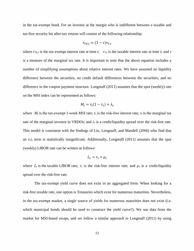
in the tax-exempt bond. For an investor at the margin who is indifferent between a taxable and
tax-free security his after-tax returns will consist of the following relationship:
𝑟𝑇𝐸,𝑡 = (1 − 𝜏)𝑟𝑇,𝑡
where rTE,t is the tax-exempt interest rate at time t; rT,t is the taxable interest rate at time t; and τ
is a measure of the marginal tax rate. It is important to note that the above equation includes a
number of simplifying assumptions about relative interest rates. We have assumed no liquidity
difference between the securities, no credit default differences between the securities, and no
difference in the coupon payment structure. Longstaff (2011) assumes that the spot (weekly) rate
on the MSI index can be represented as follows:
𝑀𝑡 = 𝑟𝑡(1 − 𝜏𝑡) + 𝜆𝑡
where Mt is the tax-exempt 1-week MSI rate; rt is the risk-free interest rate; τt is the marginal tax
rate of the marginal investor in VRDOs; and λt is a credit/liquidity spread over the risk-free rate.
This model is consistent with the findings of Liu, Longstaff, and Mandell (2006) who find that
an rtλt term is statistically insignificant. Additionally, Longstaff (2011) assumes that the spot
(weekly) LIBOR rate can be written as follows:
𝐿𝑡 = 𝑟𝑡 + 𝜇𝑡
where Lt is the taxable LIBOR rate; rt is the risk-free interest rate; and µt is a credit/liquidity
spread over the risk-free rate.
The tax-exempt yield curve does not exist in an aggregated form. When looking for a
risk-free taxable rate, one option is Treasuries which exist for numerous maturities. Nevertheless,
in the tax-exempt market, a single source of yields for numerous maturities does not exist (i.e.
which municipal bonds should be used to construct the yield curve?). We use data from the
market for MSI-based swaps, and we follow a similar approach to Longstaff (2011) by using

12
swaps where the percentage of floating LIBOR rate is exchanged for the floating MSI rate. Using
fixed-for-floating interest rate swaps based on LIBOR and MSI, we synthetically create the
LIBOR percentage basis swaps. Following the method outlined in Longstaff (2011), we create a
synthetic basis swap by using the percentage of a fixed leg of a LIBOR-based interest rate swap
required to pay the fixed leg amount of the fixed leg of a MSI-based interest rate swap. We end
up with a percentage-of-LIBOR for MSI swap. These interest rate basis swaps are generally
priced in the swap market based on the percentage of LIBOR paid/received. These swaps serve
as a direct proxy for one minus the marginal tax rate.
There are many reasons to assume that swaps offer a better measure of rates than bond
yields--particularly in the tax-exempt market. Since interest rate swaps are based on short-term
rates, the fixed leg of a swap tends to reflect the expected accumulation of realized short-term
rates. This avoids preferred habitat problems which may be embedded in the yield curve. This
also keeps embedded optionality from entering into pricing. Even if tax-exempt bonds are not
putable or callable, the issuer still holds the option of defeasance. Even for issuers of the highest
quality, defeased bonds have an altered set of risk characteristics. Swaps avoid this complication.
The swaps used here are widely traded in a standardized form so liquidity is not a problem.
We do not estimate the values of the credit/liquidity spreads shown above. Longstaff
(2011) finds the average credit/liquidity spread over the risk-free rate for the short-term MSI rate
of 0.00565 with a standard deviation of 0.00621. This is two orders of magnitude smaller than
numerous estimates of the implied tax rate. Structurally, there is far less default risk in swaps as
opposed to bonds. Bonds have a principal amount that is exchanged at maturity, but interest rate
swaps typically do not exchange the notional amount. The zero-sum game structure of interest
rate swaps makes them ideal for effective symmetric hedging. If these swaps are used for

13
hedging, then losses on the swaps should be offset by gains elsewhere on the entity’s balance
sheet. Interest rate swaps also tend to be over-collateralized further decreasing default risk.
Unlike municipal bonds which tend to be illiquid, swaps and the indices on which they are based
are widely traded in a standardized form reducing the liquidity portion of the spread.
We are primarily interested in the behavior of the proportion of tax-exempt to taxable
interest rate swaps as these give a proxy for the relative profitability of investing in taxable
versus tax-exempt markets (from here on we refer to this variable as the taxproxy).
𝑠𝑇𝐸;𝑡,𝑇
𝑠𝑇;𝑡,𝑇= 𝑡𝑎𝑥𝑝𝑟𝑜𝑥𝑦𝑡,𝑇 ≈ (1 − 𝜏)
where sTE,t,T is the swap fixed rate for a tax-exempt T-year swap at time t (MSI); sT,t,T is the swap
fixed rate for a taxable T-year swap at time t (LIBOR); taxproxyt,T is our primary variable of
interest which is derived as shown above; and τ is a measure of the marginal tax rate.
The method we use to test for the existence of structural breaks in this data is based on
Bai and Perron (2003). We use a minimum distance of 2 months between breaks. Comparing the
number of structural breaks is done through Bayesian (BIC) or modified Schwarz (LWZ)
information criteria for each number of breaks. Additionally, for each number of structural
breaks the algorithm generates F-statistics that can be compared to Bai and Perron’s asymptotic
critical values to determine model significance. Because we are testing for structural breaks, we
are limited in the types of models available.
We first test each of our variables for the presence of a unit root using the Augmented
Dickey-Fuller Test (1979) beginning with 20 lagged differences (almost an entire month). Since
there is no consensus on the data generating process for our taxproxy, we use the procedure for
determining the existence of constant and time-trend variables given by Dolado, Jenkinson, and
Sosvilla-Rivero (1990). In addition to this test, we also run Lee and Straczicich’s (2003) LM test

14
for unit root with two structural breaks. Once the order of the process is known, we can establish
the time series characteristics necessary to test for structural breaks. Since the Bai-Perron method
requires the use of only autoregressive (AR) terms, we select the best AR(p) model for each
tenor of the taxproxy.
The Bai-Perron method is computationally demanding for the number of possible breaks
in our data. Based on a recommendation from Bai and Perron’s paper, we limit the number of
structural breaks to five. Since the above set of tests relies on having non-constant means, it is
reasonable that the series may also have non-constant variance. If GARCH effects are present,
then they will reduce the power of structural break tests. However, all structural break tests had
p-values smaller than 1%. The tests for GARCH effects are included in the appendix.
Our dataset contains I(1) variables which can be combined in a way to form an I(0)
variable indicating the presence of cointegration. The presence of cointegration shows that rates
are related and driven to long run levels. To make the time series of swap rates compatible with
cointegration, a log transformation must be used. Recall that our model of the taxproxy is as
follows:
)1(,
,;
,; Tt
TtT
TtTEtaxproxy
s
s
We know that equilibrium swap rates individually are I(1) series, whereby they do not
have a mean and they are not covariance stationary over time. The time series of the taxproxy is
I(0) under the unit root test so we know that the above relationship between I(1) variables yields
a stationary series. Cointegration requires that some linear combination of less stationary series
yields a more stationary series. Taking the natural log of the above equation gives the vector:
TtTtTTtTE taxproxyss ,,;,; lnlnln

15
Implied tax rates are cyclical, so as rates decrease the implied marginal tax rates tend to
decrease. In order to allow our regression to incorporate these effects, we relax the above
restrictions on the swap rates and constraining the taxproxy to be a constant:
0lnln 0,;2,;1 TtTTtTE ss
In the above equation γi is the estimated coefficient. By using the above equation as the error
correction function, we can test for the level effects or arbitrage relationship between the
different swap rates. We follow the Engle-Granger methodology (1987) for identification and
testing. We test the natural logarithm of the fixed-leg swap rates for a unit root and confirm that
they are I(1). We solved for the coefficients in the above equation in order to determine the long
run relationship between the MSI-based swap rate and the LIBOR-based swap rate. Next, we test
for residual auto-correlation to confirm this long term relationship. We estimate a VAR type
model as shown below:
TtTE
n
i
TtT
n
i
TtTETtTTtTETETtTE
si
sisss
,;
1
,;12
1
,;110,;2,;1,;
)(
)()lnln(
TtT
n
i
TtT
n
i
TtTETtTTtTETTtT
si
sisss
,;
1
,;22
1
,;210,;2,;1,;
)(
)()lnln(
In the above equations αii is the estimated coefficient in the VAR EC model. Once the above
models are estimated the level of error correction can be calculated and checked for statistical
significance. Here again the presence of structural breaks will bias our results downward causing
the estimated level of mean reversion towards the error-correction vector to be attenuated.

16
2.3.2. Data
We obtain daily forward filled swap market data for the typically traded maturities (1, 2,
3, 4, 5, 7, 10, 15, 20, and 30-year maturities) of LIBOR (London Interbank Offer Rate) and MSI
(Securities Industry and Financial Markets Association’s Municipal Swaps Index). Weekend
observations are omitted for all of our work. A plain vanilla LIBOR swap is typically settled
semi-annually with the fixed leg being paid on a 30/360 day count convention so that each of the
payments is identical. The floating leg of the swap is paid based semiannually on an actual/360
day count convention.5 The rate used for the settlement of municipal swaps is the Municipal
Swap Index (MSI). This rate is developed by Municipal Market Data which is a subsidiary of
Thomson Financial Services. The MSI rate is based on high grade, 7-day-resettable, tax-exempt
variable rate demand obligations (VRDOs). The value of this index is determined by a market
clearing mechanism through a remarketing agent. To be included in this index, a VRDO must be
larger than $10 million. Its issuer must also have the highest short-term issuer credit rating
(VMIG1 by Moody’s or A-1+ by Standard and Poor’s). The VRDO must, also, be settled on
Wednesday. The primary owners of these securities are money market funds which are, in turn,
held by individuals (70% based on estimates by Criscuolo and Faloon, 2007). MSI is used as the
floating rate in the fixed-for-floating interest rate swaps representing tax-exempt rates. An
important note on these municipal swaps is that cash flows from these swaps are fully taxable but
the underlying rates are not.
5Although recently there have been accusations of fraud in the setting of LIBOR, these swaps are
still widely traded; and a replacement for the basis swaps has not appeared.

17
2.4. Empirical Results
2.4.1 Descriptive Statistics
The primary variables of interest for our study are the daily observations of the swap
curves for the commonly observed swap market quotations. It is important to note that our
taxproxy displays far more stationarity than either of the fixed-for-floating rates from which it is
derived. This can be seen in the serial correlations which are slightly lower for our proxy and the
variance, which is much smaller shown in Table 2.1. Our proxy follows the basis swaps in
Longstaff (2011). In results not shown, we compare descriptive statistics for the same time
period as Longstaff’s paper. They are almost exactly the same, but since he uses observed basis
swap rates some slight discrepancy is expected. For the time period used in our tests we observe
higher serial correlation and standard deviation. Both of which can be explained by structural
breaks that make an otherwise stationary series appear to be less stationary.
In order to look more specifically at the structural breaks not due to changing tax laws,
we use only prices after January 1, 2003 because previous years saw changes in the highest
marginal tax rate. Our data set covers more than seven years where the highest marginal tax rates
did not change, allowing for a test of structural breaks in the absence of tax law changes.
2.4.2. Unit Root Testing
The unit root testing was first done with the swap rates. We followed a general-to-
specific methodology by first identifying the appropriate number of differenced lag lengths as
follows:
t
n
i ititt yyy 11
Here γ is the key test statistic for our unit root test, the βi’s are the coefficients on the lagged first
differences, and yt is our variable of interest. We did not use a constant or a time term in these

18
regressions. The swap rates theoretically should not have any deterministic drift over time.
Starting with 20 lagged values, we narrowed our regressions down using t-tests until the longest
lag was significant at the 5% level. We then used the Dickey-Fuller critical values to evaluate the
existence of a unit root. In Table 2.2, we estimate the above regression for the optimum number
of coefficients and record the coefficients and their t-statistics.
We estimate these regressions over the entire sample period and identify the MSI series,
the ln(MSI) series, the LIBOR series, and the ln(LIBOR) series as containing a unit root because
we fail to reject the null hypothesis that the lag coefficient is zero. When using the first
difference of each series, we strongly reject the null hypothesis that the differenced series contain
a unit root. Together these results indicate that the MSI series, the ln(MSI) series, the LIBOR
series, and the ln(LIBOR) series are each I(1) series. We move next to the unit root testing of the
taxproxy.
There are several issues with testing the taxproxy for the presence of a unit root. Since the
presence of structural breaks can cause a stationary series to fail to reject the null hypothesis of a
unit root, the rejection of a unit root is a stronger test than required for the use of the Bai-Perron
procedure. Since there is no consensus in the literature on the characteristics of our data
generating function, taxproxy, we use the Dolado, et al. (1990) procedure that assumes that the
data generating process is completely unknown. This method begins by estimating the following
equation:
t
n
i ititt ytayay 1210
Here a0 is the constant term, and a2 is the drift coefficient. The optimum number of lags is found
in the same way as described above. In results not shown, we eliminate the presence of a
constant and time trend term. From 2003 to the end of our sample period, this tests also fails to

19
reject initially, then rejects at first differences, indicating that each tenor of the taxproxy is an I(1)
process. However, we later find that there are multiple significant structural breaks in this
variable. To incorporate the presence of structural breaks, we run the Lee-Strazicich’s (2003)
minimum LM unit root test with two structural breaks. The presence of structural breaks can
cause the Dickey-Fuller test to fail to reject, but “a rejection of the null unambiguously implies
trend stationarity” under Lee and Strazicich’s test. The results for a change in just the level are
shown in Table 2.3.
In a number of tenors, our results show that the series are stationary with structural
breaks. Additionally, each model selects the maximum two structural breaks allowed under this
model. Since more structural breaks are present, it is likely that the failure to reject in the longer
tenors is due to the need to include the additional breaks. To be thorough, we also test using a
model that allows for breaks in both the level and slope terms.
Later tests with the Bai-Perron methodology show that we have structural breaks in both
the level and AR terms, so we also run Lee and Strazicich’s Test with this specification. When
structural breaks are present, the Lee and Strazicich Test’s critical values are dependent on the
location of the breaks. The locations are given by the fraction of the time series’ data points that
have occurred before the break date for each break. Since all of our break locations with two
breaks are above 0.4 for the first break and 0.6 for the second break, we use the critical values,
from Table 2 in Lee and Strazicich’s paper, for the following break locations to create a plane:
(0.4, 0.6), (0.4, 0.8), and (0.6, 0.8). The plane that we create is in three dimensions, with the
locations of the first and second breaks being two dimensions, and the 1 or 10% critical values
being the third dimension. By doing this, we can linearly interpolate all of the necessary critical
values for our tests. The results from this test along with critical values are shown in Table 2.4.

20
Table 2.4 shows that over a number of shorter tenors, we reject the null hypothesis in
favor of a stationary series with structural breaks. Based on the reported critical values, we
cannot reject for the longer tenors, but two issues arise: the low n for our critical values and the
known presence of additional structural breaks. The critical values given in Lee and Strazicich’s
paper are for 100 observations, making them further from zero than if the critical values were for
the 2000 observations used in our analysis. Generating these new critical values is
computationally untenable because the LS test is quite computationally demanding.6 In our later
analysis, we find between 3 and 5 structural breaks in our series. The setup for the LS test does
allow for more than two structural breaks but the computational time required grows
exponentially with each additional break making this too unviable. The addition of these effects
will increase the likelihood that we select a model that is stationary with structural breaks
moving us toward our conclusion. We next move to see if the MSI-based fixed-leg rates and the
LIBOR-based fixed-leg rates move together.
2.4.3. Cointegration Model
One can argue that the co-movement of these rates is simply an artifact of each rate
having a similar tenor and that these rates are not in fact related. As a robustness test, we run a
cointegration model to see if these rates actually do move together in a statistically significant
way as previous theory indicates. The existence of a semi-arbitrage type relationship is ideal for
a cointegration model. A cointegration model is useful for considering two processes that are
each themselves unit root processes but have some relationship to each other (like never moving
too far apart from each other). Cointegration depends on a linear combination of variables. To
6We calculated that it would take 4.59 years to generate a single critical value for 2000
observations with one of our office computers.
21
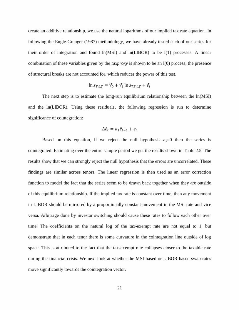
create an additive relationship, we use the natural logarithms of our implied tax rate equation. In
following the Engle-Granger (1987) methodology, we have already tested each of our series for
their order of integration and found ln(MSI) and ln(LIBOR) to be I(1) processes. A linear
combination of these variables given by the taxproxy is shown to be an I(0) process; the presence
of structural breaks are not accounted for, which reduces the power of this test.
ln 𝑠𝑇;𝑡,𝑇 = 𝛾0̂ + 𝛾1̂ ln 𝑠𝑇𝐸;𝑡,𝑇 + 𝑒�̂�
The next step is to estimate the long-run equilibrium relationship between the ln(MSI)
and the ln(LIBOR). Using these residuals, the following regression is run to determine
significance of cointegration:
∆�̂�𝑡 = 𝑎1�̂�𝑡−1 + 휀𝑡
Based on this equation, if we reject the null hypothesis a1=0 then the series is
cointegrated. Estimating over the entire sample period we get the results shown in Table 2.5. The
results show that we can strongly reject the null hypothesis that the errors are uncorrelated. These
findings are similar across tenors. The linear regression is then used as an error correction
function to model the fact that the series seem to be drawn back together when they are outside
of this equilibrium relationship. If the implied tax rate is constant over time, then any movement
in LIBOR should be mirrored by a proportionally constant movement in the MSI rate and vice
versa. Arbitrage done by investor switching should cause these rates to follow each other over
time. The coefficients on the natural log of the tax-exempt rate are not equal to 1, but
demonstrate that in each tenor there is some curvature in the cointegration line outside of log
space. This is attributed to the fact that the tax-exempt rate collapses closer to the taxable rate
during the financial crisis. We next look at whether the MSI-based or LIBOR-based swap rates
move significantly towards the cointegration vector.

22
We add error-correction behavior to a VAR model in order to see if divergence from
long-run behavior causes the series to move back together. Alternatively, we ask the question: is
the error correction vector significant in regressions with the taxable rate on the LHS, regressions
with the tax-exempt rate on the LHS, both regressions? Using the error correction vectors for
each tenor, we compute a VAR style model with lags of the natural logarithm of the first
difference of the MSI-based and LIBOR-based series. Lag lengths are found using the BIC.
In Table 2.6, we find that at the shortest tenors, the error correction vector coefficient is
significant only in the LIBOR equation. As we move past a four year tenor, the error correction
vector coefficient becomes significant, but only in the MSI equation. It seems that for short
tenors the LIBOR swap rates error correct towards the MSI swap rates, and for long tenors the
MSI moves towards the LIBOR. This error correction is of similar magnitude in both variables.
At higher magnitudes the error correction terms for the LIBOR are negative, which shows these
variables moving away from each other. However, these terms are also not statistically
significant so we cannot say that they are not zero. Even with significant structural breaks across
all tenors, the normal pattern for these markets is for them to error correct (significantly in one
market or the other except for the four year tenor). An examination of the t-statistics indicates
that in every case except for the thirty year tenor, these time series Granger-Cause each other. In
the thirty year tenor, the LIBOR Granger-Causes MSI but not vice versa. Here again we see
significant evidence that these rates are highly related. Each of these ECM implies an impulse
response function which we show in Figure 2.2.
The impulse responses show that these equations contain a small but long-run level of
persistence. This is also consistent with our knowledge of interest rates. Interest rates and related
instruments tend to display unit-root behavior in the short-term and mean-reversion over long
23
periods of time (Cochrane, 1991). Having shown that these rates are significantly cointegrated
even in the presence of structural breaks, we move to structural break testing.
2.4.4. Structural Break Testing
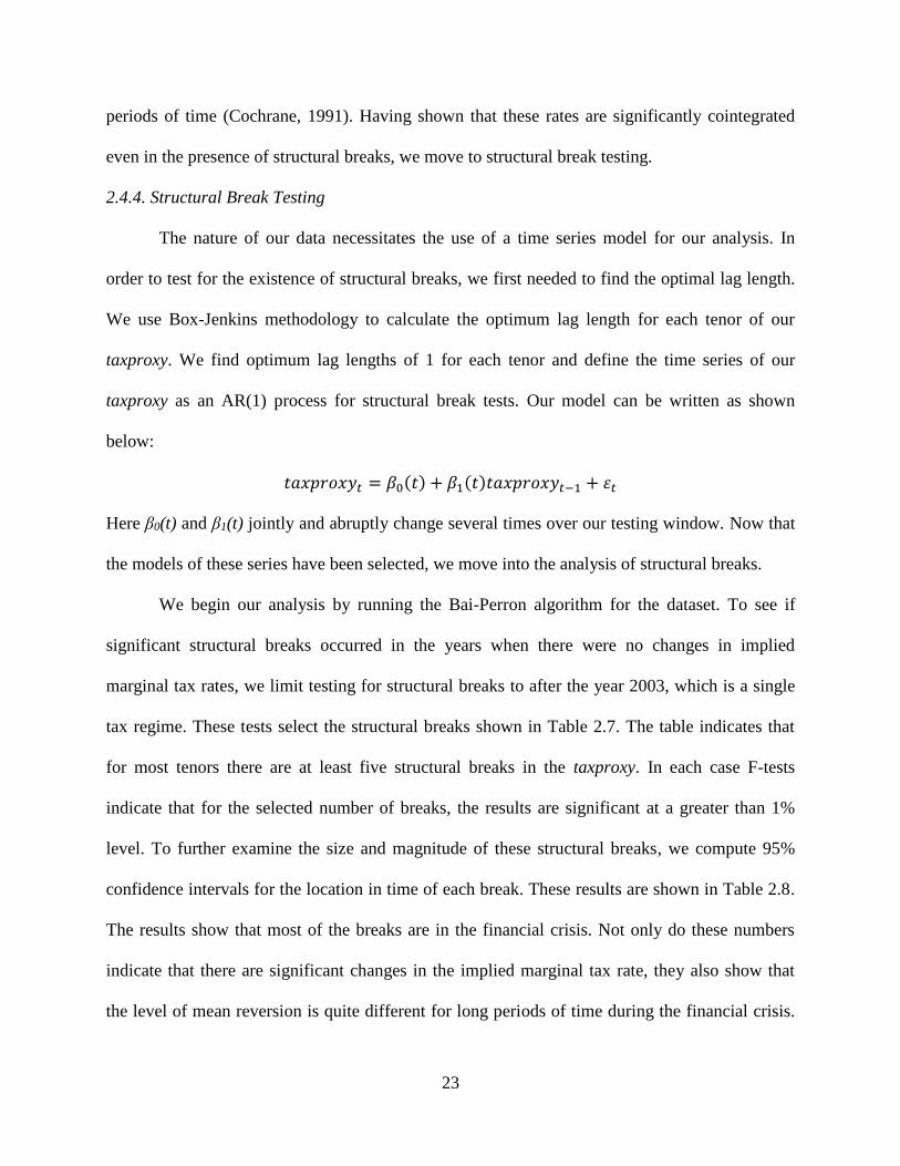
The nature of our data necessitates the use of a time series model for our analysis. In
order to test for the existence of structural breaks, we first needed to find the optimal lag length.
We use Box-Jenkins methodology to calculate the optimum lag length for each tenor of our
taxproxy. We find optimum lag lengths of 1 for each tenor and define the time series of our
taxproxy as an AR(1) process for structural break tests. Our model can be written as shown
below:
𝑡𝑎𝑥𝑝𝑟𝑜𝑥𝑦𝑡 = 𝛽0(𝑡) + 𝛽1(𝑡)𝑡𝑎𝑥𝑝𝑟𝑜𝑥𝑦𝑡−1 + 휀𝑡
Here β0(t) and β1(t) jointly and abruptly change several times over our testing window. Now that
the models of these series have been selected, we move into the analysis of structural breaks.
We begin our analysis by running the Bai-Perron algorithm for the dataset. To see if
significant structural breaks occurred in the years when there were no changes in implied
marginal tax rates, we limit testing for structural breaks to after the year 2003, which is a single
tax regime. These tests select the structural breaks shown in Table 2.7. The table indicates that
for most tenors there are at least five structural breaks in the taxproxy. In each case F-tests
indicate that for the selected number of breaks, the results are significant at a greater than 1%
level. To further examine the size and magnitude of these structural breaks, we compute 95%
confidence intervals for the location in time of each break. These results are shown in Table 2.8.
The results show that most of the breaks are in the financial crisis. Not only do these numbers
indicate that there are significant changes in the implied marginal tax rate, they also show that
the level of mean reversion is quite different for long periods of time during the financial crisis.

24
This evidence casts doubt on models that assume a single stable implied marginal tax rate for a
given tax regime and on models that assume a mean reverting implied marginal tax rate. To
quantify the economic significance of these structural breaks, we take the fixed leg values at each
side of the 95% confidence intervals shown in Table 2.9.
These structural breaks are statistically and economically significant given the large
notional value for this instrument. The statistical significance of these breaks has been
established through the use of Bai-Perron critical values so even though some of the taxproxy
changes are small, they are still significant at the 1% level. Looking at the 1-year tenor, we find
that multiple significant structural breaks have occurred within a single tax regime. This is
consistent with tax effects previously documented in the literature (i.e. the Steve Forbes effect on
implied tax rates). In contrast to Greimel and Slemrod (1999), who found no significant effects
on the long run implied tax rates, we find that the 30-year tenor shows statistically and
economically significant changes. These changes are in the absence of tax regime changes, and
they are quite large. In November 2008, the implied marginal tax rate dropped 15.3% and in
April 2009 the implied marginal tax rate rose 10.8%. We now outline several factors that may
have led to these structural breaks.
2.5. Discussion
The structural breaks happened for different reasons than those outlined in the previous
literature. These years did not see changing tax regimes. Outlined below are several explanations
for the changes found in this paper.
The flow of funds during the recent financial crisis is one possible explanation for the
significant structural breaks in the implied marginal tax rate. Since MSI is used for investment
25
purposes for individuals, those moving their funds out of tax-exempt investments would
influence prices. We expect to see funds move from tax-exempt to taxable as individuals change
their investment behavior due to lower expected tax liabilities. Suppose that a large number of
investors realize near the end of 2008 (or when they are filling their taxes) that their large losses
will materially affect their marginal tax rate. This change in individual marginal tax rates could
cause them to change their investment behavior to maximize their after tax returns, and could
account for the additional shifts observed in 2009 and 2010. In order to see if fund flows line up
with the structural breaks, a number of different transformations were tested. None of these
transformations, first differences, or proportional measures yielded any pattern consistent with
the structural breaks in the implied marginal tax rates which are shown in Figures 2.3 and 2.4.
Another potential argument for the observed structural breaks is changing credit
conditions. The frequency of many of these deviations indicates that this is unlikely to be the
case. Additionally, the underlying municipal swap rate is based on seven day resettable
securities. The short duration of these securities means that they can respond quickly to changing
credit conditions, but the fact that the index includes only issuers with the highest rating
available for short-term issuers casts doubt on this explanation. Appleson, et al. (2012) show in
Table 2.10 that although there have been a large number of defaults in the municipal bond
market, there are very few among rated issuers. Table 2.10 shows that there have been less than
118 municipal defaults from issues rated by S&P and Moody’s between 1970 and 2011. In a
larger sample of rated and unrated municipal issuers, there exists some clustering during the
recent financial crisis. During the recent financial crisis, a number of bond insuring agencies lost
their high credit ratings and some municipal issuers lost their credit guaranties. By definition, the
MSI adjusts for these effects by only including VRDOs with issuers that have the highest

26
possible short-term credit rating. The drop in available highly-rated issuers could explain some
of the variation, but we would expect movement in a single direction. The rare nature of rated
municipal default implies that a changing credit environment is unlikely to explain the observed
structural breaks.
There is also an argument that these results are driven by the supply of tax-exempt bonds.
In order to look at the supply effects, we pull IRS records for the number and mount of tax-
exempt governmental bonds each year which is shown in Table 2.11. Tax-exempt private
activity bonds are still subject to the AMT so they are not included in this number. The amount
of issuances is highest in 2003 and 2009. The IMTRs observed in 2003 are for many tenors some
of the highest IMTRs. The IMTRs observed in 2009 are some of the lowest observed in our
analysis. Hence, a supply side story does not fit our observed structural breaks. This additional
evidence is again consistent with changing investor tax situations through the financial crisis.
A recent paper by Mitchell and Pulvino (2012) shed light on fire sales done by
rehypothecation lenders during the recent financial crisis. They use a number of proprietary data
sources to illustrate the collapse of several different types of quasi-arbitrage trading strategies
often used by hedge funds. In the weeks following the Lehman Brothers’ bankruptcy, the market
for short term financing almost completely disappeared and at the same time lenders attempted to
liquidate their collateral holdings. This caused a number of quasi-arbitrage trades to diverge from
their long-run levels for months until new capital arrived to trade on almost certainly profitable
trading opportunities. In the same vein, there is an expected long-run mean for the implied
marginal tax rate. Figure 1 shows that in 2006 and most of 2007 the taxproxy is almost flat. In
2008 the taxproxy fluctuates wildly at around the same time the short term financing market

27
dried up. The limited leverage available to exploit arbitrage opportunities is one likely
explanation for the persistence observed structural breaks.
2.6. Conclusion
We document several structural breaks that have occurred in the implied marginal tax
rate as observed from MSI-based and LIBOR-based swap markets. These structural breaks are
statistically significant under Bai and Perron’s methodology and are also economically
significant. We trace major changes to both the taxable and tax-exempt markets. An important
consideration going forward is that these breaks tend to occur during times of economic
downturn.
This information could be used as a macroeconomic hedge. If these rates diverge away
from their long-run means in a predictable way, an entity that depends on taxes could enter into a
basis swap that increases in value during times of lower tax revenues and correspondingly lower
implied tax rates. Additionally, our results cast doubt on the use of numerous short-rate models.
Structural changes have been predicted in the previous literature between different tax regimes,
but we have shown that in the absence of tax regimes, structural breaks in the implied tax rate
have still occurred. This challenges the effectiveness of short-rate models in applications over
long periods of time. Our findings also indicate that future studies of asset pricing between
taxable and tax-exempt asset pricing must have some way of controlling for clientele changes
because the economic climate can significantly change the distribution of tax filers based on
where they are in different tax brackets.

28
REFERENCES
Appleson, J., Parsons, E., & Haughwout, A. (2012). The untold story of municipal bond defaults.
Liberty Street Economics, Federal Reserve Bank of New York.
Bai, J. & Perron, P. (2003). Computation and analysis of multiple structural change models.
Journal of Applied Econometrics 18, 1-22.
Brooks, R. (1999). Municipal bonds: a contingent claims perspective. Financial Services Review.
8(1), 71-85.
Brooks, R. (2002). The cost of tax policy uncertainty: evidence from the municipal swap market.
The Journal of Fixed Income 12, 71-87.
Brooks, R., Cline, B. N., & Enders, W. (2012). Information in the U.S. Treasury term structure
of interest rates. The Financial Review 47, 247–272.
Chalmers, J.M.R. (1998). Default risk cannot explain the muni puzzle: evidence from municipal
bonds that are secured by U.S. Treasury obligations. Review of Financial Studies 11(2), 281-
308.
Chalmers, J.M.R. (2006). Systematic risk and the muni puzzle. National Tax Journal 59(4), 833-
848.
Cochrane, J. H. (1991). Pitfalls and opportunities: what macroeconomists should know about
unit roots. NBER Macroeconomics Annual 6, 201-210.
Criscuolo, A. & Faloon, M. (2007). Variable rate demand obligations. Research Report, Standish
Mellon Asset Management.
DeAngelo, H. & Masulis, R. (1980). Optimal capital structure under corporate and personal
taxation. Journal of Financial Economics 8, 3-29.
Dickey, D. & Fuller, W. (1979). Distribution of the estimates for autoregressive time series with
a unit root. Journal of the American Statistical Association 74, 427-231.
Dolado, J., Jenkinson, T., & Sosvilla-Rivero, S. (1990). Cointegration and unit roots. Journal of
Economic Surveys 4, 249-273.

29
Engle, R. & Granger, C. (1987). Cointegration and error-correction: representation, estimation,
and testing. Econometrica 55, 251-276.
Fama, E. (1984a). The information in the term structure. Journal of Financial Economics 13,
509-528.
Fama, E. (1984b). Term premiums in bond returns. Journal of Financial Economics 13, 529-546.
Green, R. (1993). A simple model of taxable and tax-exempt yield curves. The Review of
Financial Studies 6(2), 233-264.
Greimel, T. & Slemrod, J. (1999). Did Steve Forbes scare the U.S. municipal bond market?
Journal of Public Economics 74(1), 81-96.
Johansen, S. (1988). Statistical analysis of cointegration vectors. Journal of Economic Dynamics
and Controls 12, 231-254.
Kassouf, S. & Thorp, E. (1990). Beat the Market. Random House, New York.
Lee, J. & Strazicich, M. (2003). Minimum Lagrange Multiplier Unit Root Test with Two
Structural Breaks. The Review of Economics and Statistics 85, 1082-1089.
Liu, J., Longstaff, F., & Mandell, R. (2006). The market price of risk in interest rate swaps: The
roles of default and liquidity risks. Journal of Business 79, 2337–2359.
Longstaff, F. (2011). Municipal debt and marginal tax rates: is there a tax premium in asset
prices? Journal of Finance 61(3), 721-751.
McLeod, A. & Li, W. (1983). Diagnostic checking ARMA time series models using squared
residual correlations. Journal of Time Series Analysis 4, 269-273.
McNulty, J. & Smith, S. (1998). Correlated interest rate risk and funding strategies for
nonfinancial firms. The Financial Review 33(1), 31-44.
Mitchell, M. & Pulvino, T. (2012). Arbitrage crashes and the speed of capital. Journal of
Financial Economics 104, 469-490.
Nelson, C. & Siegle, A. (1987). Parsimonious modeling of yield curves. Journal of Business 60,
473-489.
Perron, P. (1997). Further evidence on breaking trend functions in macroeconomic variables.
Journal of Econometrics 80(2), 355-385.

30
2.A. APPENDIX
2.A.1. GARCH Effects
There exist several ways to pretest for generalized autoregressive conditional
heteroskedasticity. The presence of non-constant variance is fairly common in financial variables
which generally behave as GARCH(1,1) processes. We take each of the variables and
individually test for these types of nonlinear effects. Then the best GARCH process for each
series is found by using as a starting point the best ARIMA process and then adding different
GARCH characteristics. Since their means move together, it is plausible that the variance of the
tax-exempt rate moves with the variance of the taxable rate. A multivariate GARCH model of
the lagged differenced tax-exempt series and the lagged differenced taxable series are used. We
show here some multivariate GARCH models of the 1-year maturity. If the differences move
together and the variances move together, then it is possible that the series are cointegrated. If
GARCH effects are present, then they will reduce the power of structural break testing.
However, since our tests for structural breaks resulted in highly statistically significant results,
we ignore these effects in the body of our paper.
The variables used to create the cointegration vector were also found to have GARCH
effects. Testing for different types of univariate GARCH effects indicated an IGARCH(1,1)
model for Δln(LIBOR) and Δln(MSI). Model selection was done using AIC and BIC. One
problem with the these observed effects is that under the arbitrage relationship described earlier,
there will be a group of investors who will have an incentive to switch their investments back
and forth depending on their expected marginal tax rate. The univariate GARCH models shown
below do not capture any type of volatility spillover, but multivariate GARCH models did show

31
significant spillover effects. Because we are primarily focused on the data generating process of
the means, we do not show the variance effects.
To give a description of the variance of the series in this study, we begin by pretesting
our series for nonlinear effects by using the McLeod-Li test (1983). Each of the tenors of the
taxproxy variables shows significant autocorrelation in the squared residuals indicating GARCH
effects. The presence of these effects reduces the power of structural break tests. Much of the
GARCH effects are concentrated in the fourth lag likely because the underlying rate on the
municipal swap, MSI, is settled weekly. These results are shown in Table 2.A.1. Since structural
break tests were highly statistically significant in the presence of GARCH effects, there is no
reason to try to control for them in our main results.
2.A.2. Structural Breaks Related to Tax Regime Changes
We have put forward that our work is the first to find structural breaks within a single tax
regime. This presupposes that a tax regime change will involve a structural break in implied tax
rates. In order to test this idea, we use several other datasets. The data set used for this paper goes
back to April 20, 2001. The “Bush Tax Cuts”7 caused the highest marginal tax rate to decline
over 3 years: 39.6% in 2000, 39.1% in 2001, 38.6% in 2002, and 35.0% in 2003. The first law in
this set had tax rates declining over a 5 year period, but the second law signed in 2003 had these
tax cuts completed in 2003. The turn of the century saw the collapse of the dot-com bubble,
which is a contravening effect present in this time period. Figure 2.A.1 gives an overview of our
taxproxy’s movements over these years. An upward movement on this graph is the same as a
lower implied marginal tax rate. Correspondingly, the shorter-term implied tax rate is lower in
7 The Economic Growth and Tax Relief Reconciliation Act signed in May 2001, and Jobs and
Growth Tax Relief Reconciliation Act signed in May 2003.
32
2003 than in the previous years. The results in Table 2.A.2 show structural breaks that are
significant at the 1% level except for the 5-year tenor which is significant at the 2.5% level. The
structural breaks and their corresponding AR(1) models are shown in Table 2.A.3.
The results show a number of significant changes in the model terms as well as long-run
means. The general trend is that our taxproxy’s long-run mean is higher in the later portion of the
time window. The chaos relating to the end of the dot-com bubble and the resultant losses in the
stock market would move many investors to a lower tax bracket. This change in investment
behavior could lead to a declining implied marginal tax rate (which in our framework would be
an increasing taxproxy). The other viewpoint is that investors, realizing that they would be
paying a lower marginal tax rate, required a higher return on their tax-exempt investments. The
results show evidence of both effects. Several spikes in the taxproxy are consistent with market
wide losses, and the overall upward trend is consistent with the predicted effects of a tax cut.
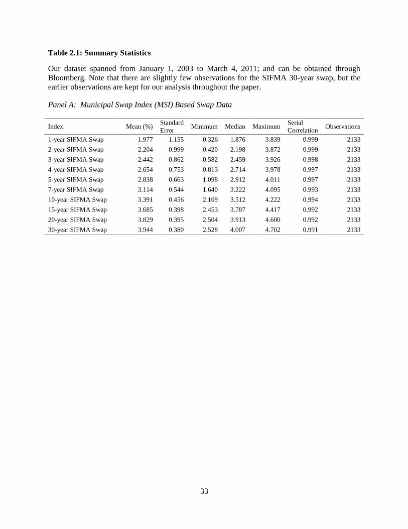
33
Table 2.1: Summary Statistics
Our dataset spanned from January 1, 2003 to March 4, 2011; and can be obtained through
Bloomberg. Note that there are slightly few observations for the SIFMA 30-year swap, but the
earlier observations are kept for our analysis throughout the paper.
Panel A: Municipal Swap Index (MSI) Based Swap Data
Index Mean (%) Standard
Error Minimum Median Maximum
Serial
Correlation Observations
1-year SIFMA Swap 1.977 1.155 0.326 1.876 3.839 0.999 2133
2-year SIFMA Swap 2.204 0.999 0.420 2.198 3.872 0.999 2133
3-year SIFMA Swap 2.442 0.862 0.582 2.459 3.926 0.998 2133
4-year SIFMA Swap 2.654 0.753 0.813 2.714 3.978 0.997 2133
5-year SIFMA Swap 2.838 0.663 1.098 2.912 4.011 0.997 2133
7-year SIFMA Swap 3.114 0.544 1.640 3.222 4.095 0.993 2133
10-year SIFMA Swap 3.391 0.456 2.109 3.512 4.222 0.994 2133
15-year SIFMA Swap 3.685 0.398 2.453 3.787 4.417 0.992 2133
20-year SIFMA Swap 3.829 0.395 2.504 3.913 4.600 0.992 2133
30-year SIFMA Swap 3.944 0.380 2.528 4.007 4.702 0.991 2133
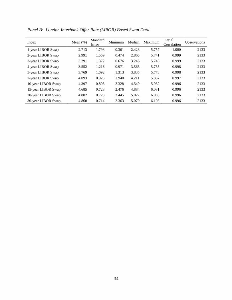
34
Panel B: London Interbank Offer Rate (LIBOR) Based Swap Data
Index Mean (%) Standard
Error Minimum Median Maximum
Serial
Correlation Observations
1-year LIBOR Swap 2.713 1.798 0.361 2.428 5.757 1.000 2133
2-year LIBOR Swap 2.991 1.569 0.474 2.865 5.741 0.999 2133
3-year LIBOR Swap 3.291 1.372 0.676 3.246 5.745 0.999 2133
4-year LIBOR Swap 3.552 1.216 0.971 3.565 5.755 0.998 2133
5-year LIBOR Swap 3.769 1.092 1.313 3.835 5.773 0.998 2133
7-year LIBOR Swap 4.093 0.925 1.940 4.211 5.837 0.997 2133
10-year LIBOR Swap 4.397 0.803 2.328 4.549 5.932 0.996 2133
15-year LIBOR Swap 4.685 0.728 2.476 4.884 6.031 0.996 2133
20-year LIBOR Swap 4.802 0.723 2.445 5.022 6.083 0.996 2133
30-year LIBOR Swap 4.860 0.714 2.363 5.079 6.108 0.996 2133
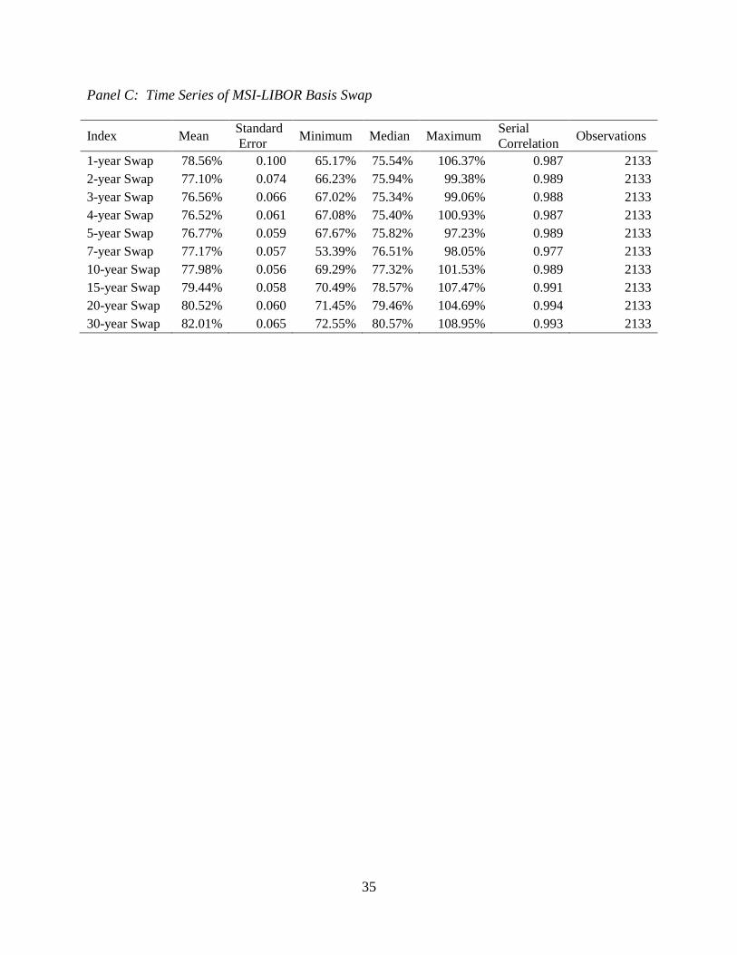
35
Panel C: Time Series of MSI-LIBOR Basis Swap
Index Mean Standard
Error Minimum Median Maximum
Serial
Correlation Observations
1-year Swap 78.56% 0.100 65.17% 75.54% 106.37% 0.987 2133
2-year Swap 77.10% 0.074 66.23% 75.94% 99.38% 0.989 2133
3-year Swap 76.56% 0.066 67.02% 75.34% 99.06% 0.988 2133
4-year Swap 76.52% 0.061 67.08% 75.40% 100.93% 0.987 2133
5-year Swap 76.77% 0.059 67.67% 75.82% 97.23% 0.989 2133
7-year Swap 77.17% 0.057 53.39% 76.51% 98.05% 0.977 2133
10-year Swap 77.98% 0.056 69.29% 77.32% 101.53% 0.989 2133
15-year Swap 79.44% 0.058 70.49% 78.57% 107.47% 0.991 2133
20-year Swap 80.52% 0.060 71.45% 79.46% 104.69% 0.994 2133
30-year Swap 82.01% 0.065 72.55% 80.57% 108.95% 0.993 2133
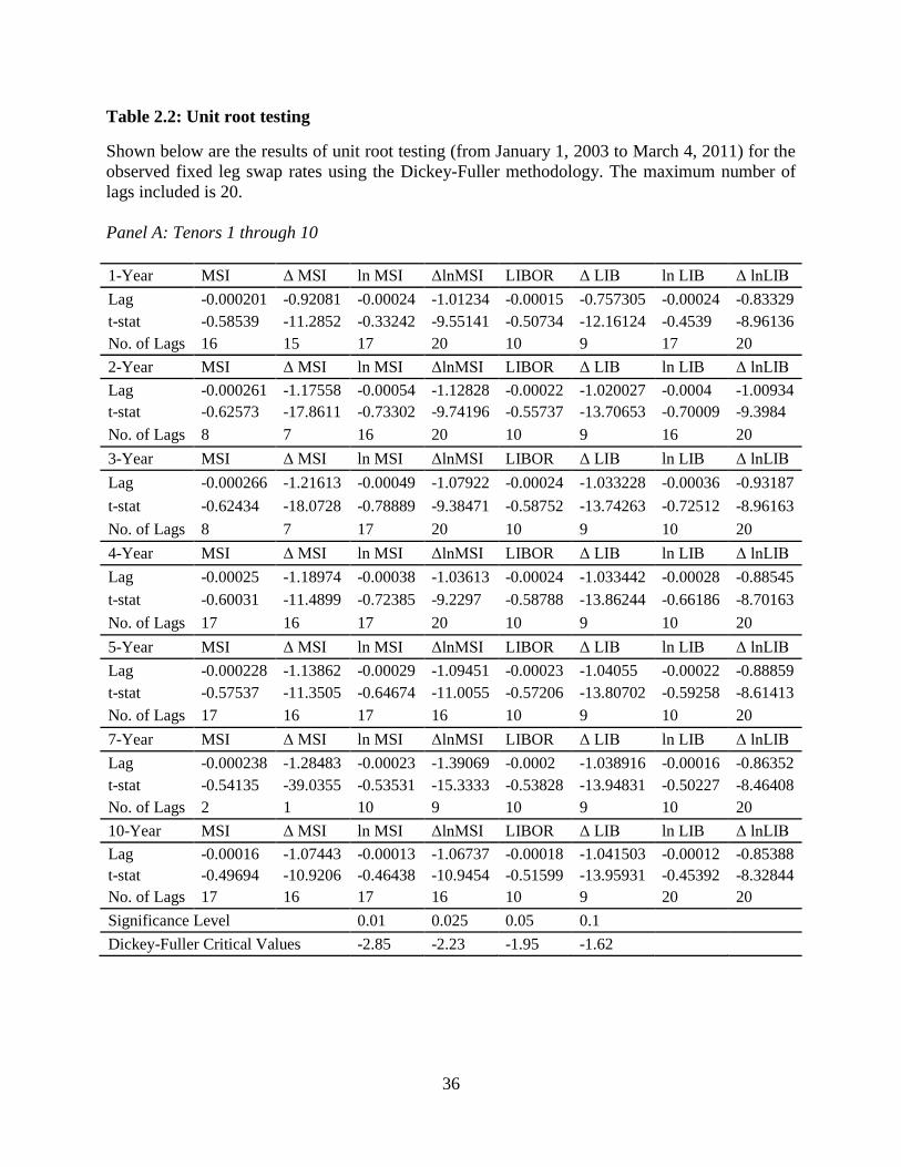
36
Table 2.2: Unit root testing
Shown below are the results of unit root testing (from January 1, 2003 to March 4, 2011) for the
observed fixed leg swap rates using the Dickey-Fuller methodology. The maximum number of
lags included is 20.
Panel A: Tenors 1 through 10
1-Year MSI Δ MSI ln MSI ΔlnMSI LIBOR Δ LIB ln LIB Δ lnLIB
Lag -0.000201 -0.92081 -0.00024 -1.01234 -0.00015 -0.757305 -0.00024 -0.83329
t-stat -0.58539 -11.2852 -0.33242 -9.55141 -0.50734 -12.16124 -0.4539 -8.96136
No. of Lags 16 15 17 20 10 9 17 20
2-Year MSI Δ MSI ln MSI ΔlnMSI LIBOR Δ LIB ln LIB Δ lnLIB
Lag -0.000261 -1.17558 -0.00054 -1.12828 -0.00022 -1.020027 -0.0004 -1.00934
t-stat -0.62573 -17.8611 -0.73302 -9.74196 -0.55737 -13.70653 -0.70009 -9.3984
No. of Lags 8 7 16 20 10 9 16 20
3-Year MSI Δ MSI ln MSI ΔlnMSI LIBOR Δ LIB ln LIB Δ lnLIB
Lag -0.000266 -1.21613 -0.00049 -1.07922 -0.00024 -1.033228 -0.00036 -0.93187
t-stat -0.62434 -18.0728 -0.78889 -9.38471 -0.58752 -13.74263 -0.72512 -8.96163
No. of Lags 8 7 17 20 10 9 10 20
4-Year MSI Δ MSI ln MSI ΔlnMSI LIBOR Δ LIB ln LIB Δ lnLIB
Lag -0.00025 -1.18974 -0.00038 -1.03613 -0.00024 -1.033442 -0.00028 -0.88545
t-stat -0.60031 -11.4899 -0.72385 -9.2297 -0.58788 -13.86244 -0.66186 -8.70163
No. of Lags 17 16 17 20 10 9 10 20
5-Year MSI Δ MSI ln MSI ΔlnMSI LIBOR Δ LIB ln LIB Δ lnLIB
Lag -0.000228 -1.13862 -0.00029 -1.09451 -0.00023 -1.04055 -0.00022 -0.88859
t-stat -0.57537 -11.3505 -0.64674 -11.0055 -0.57206 -13.80702 -0.59258 -8.61413
No. of Lags 17 16 17 16 10 9 10 20
7-Year MSI Δ MSI ln MSI ΔlnMSI LIBOR Δ LIB ln LIB Δ lnLIB
Lag -0.000238 -1.28483 -0.00023 -1.39069 -0.0002 -1.038916 -0.00016 -0.86352
t-stat -0.54135 -39.0355 -0.53531 -15.3333 -0.53828 -13.94831 -0.50227 -8.46408
No. of Lags 2 1 10 9 10 9 10 20
10-Year MSI Δ MSI ln MSI ΔlnMSI LIBOR Δ LIB ln LIB Δ lnLIB
Lag -0.00016 -1.07443 -0.00013 -1.06737 -0.00018 -1.041503 -0.00012 -0.85388
t-stat -0.49694 -10.9206 -0.46438 -10.9454 -0.51599 -13.95931 -0.45392 -8.32844
No. of Lags 17 16 17 16 10 9 20 20
Significance Level 0.01 0.025 0.05 0.1
Dickey-Fuller Critical Values -2.85 -2.23 -1.95 -1.62
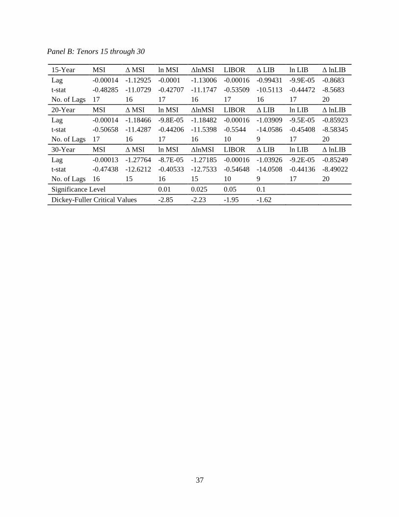
37
Panel B: Tenors 15 through 30
15-Year MSI Δ MSI ln MSI ΔlnMSI LIBOR Δ LIB ln LIB Δ lnLIB
Lag -0.00014 -1.12925 -0.0001 -1.13006 -0.00016 -0.99431 -9.9E-05 -0.8683
t-stat -0.48285 -11.0729 -0.42707 -11.1747 -0.53509 -10.5113 -0.44472 -8.5683
No. of Lags 17 16 17 16 17 16 17 20
20-Year MSI Δ MSI ln MSI ΔlnMSI LIBOR Δ LIB ln LIB Δ lnLIB
Lag -0.00014 -1.18466 -9.8E-05 -1.18482 -0.00016 -1.03909 -9.5E-05 -0.85923
t-stat -0.50658 -11.4287 -0.44206 -11.5398 -0.5544 -14.0586 -0.45408 -8.58345
No. of Lags 17 16 17 16 10 9 17 20
30-Year MSI Δ MSI ln MSI ΔlnMSI LIBOR Δ LIB ln LIB Δ lnLIB
Lag -0.00013 -1.27764 -8.7E-05 -1.27185 -0.00016 -1.03926 -9.2E-05 -0.85249
t-stat -0.47438 -12.6212 -0.40533 -12.7533 -0.54648 -14.0508 -0.44136 -8.49022
No. of Lags 16 15 16 15 10 9 17 20
Significance Level 0.01 0.025 0.05 0.1
Dickey-Fuller Critical Values -2.85 -2.23 -1.95 -1.62
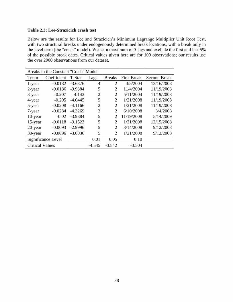
38
Table 2.3: Lee-Strazicich crash test
Below are the results for Lee and Strazicich’s Minimum Lagrange Multiplier Unit Root Test,
with two structural breaks under endogenously determined break locations, with a break only in
the level term (the “crash” model). We set a maximum of 5 lags and exclude the first and last 5%
of the possible break dates. Critical values given here are for 100 observations; our results use
the over 2000 observations from our dataset.
Breaks in the Constant "Crash" Model
Tenor Coefficient T-Stat Lags Breaks First Break Second Break
1-year -0.0182 -3.6376 4 2 3/5/2004 12/16/2008
2-year -0.0186 -3.9384 5 2 11/4/2004 11/19/2008
3-year -0.207 -4.143 2 2 5/11/2004 11/19/2008
4-year -0.205 -4.0445 5 2 1/21/2008 11/19/2008
5-year -0.0208 -4.1166 2 2 1/21/2008 11/19/2008
7-year -0.0284 -4.3269 3 2 6/10/2008 3/4/2008
10-year -0.02 -3.9884 5 2 11/19/2008 5/14/2009
15-year -0.0118 -3.1522 5 2 1/21/2008 12/15/2008
20-year -0.0093 -2.9996 5 2 3/14/2008 9/12/2008
30-year -0.0096 -3.0036 5 2 1/21/2008 9/12/2008
Significance Level 0.01 0.05 0.10
Critical Values -4.545 -3.842 -3.504
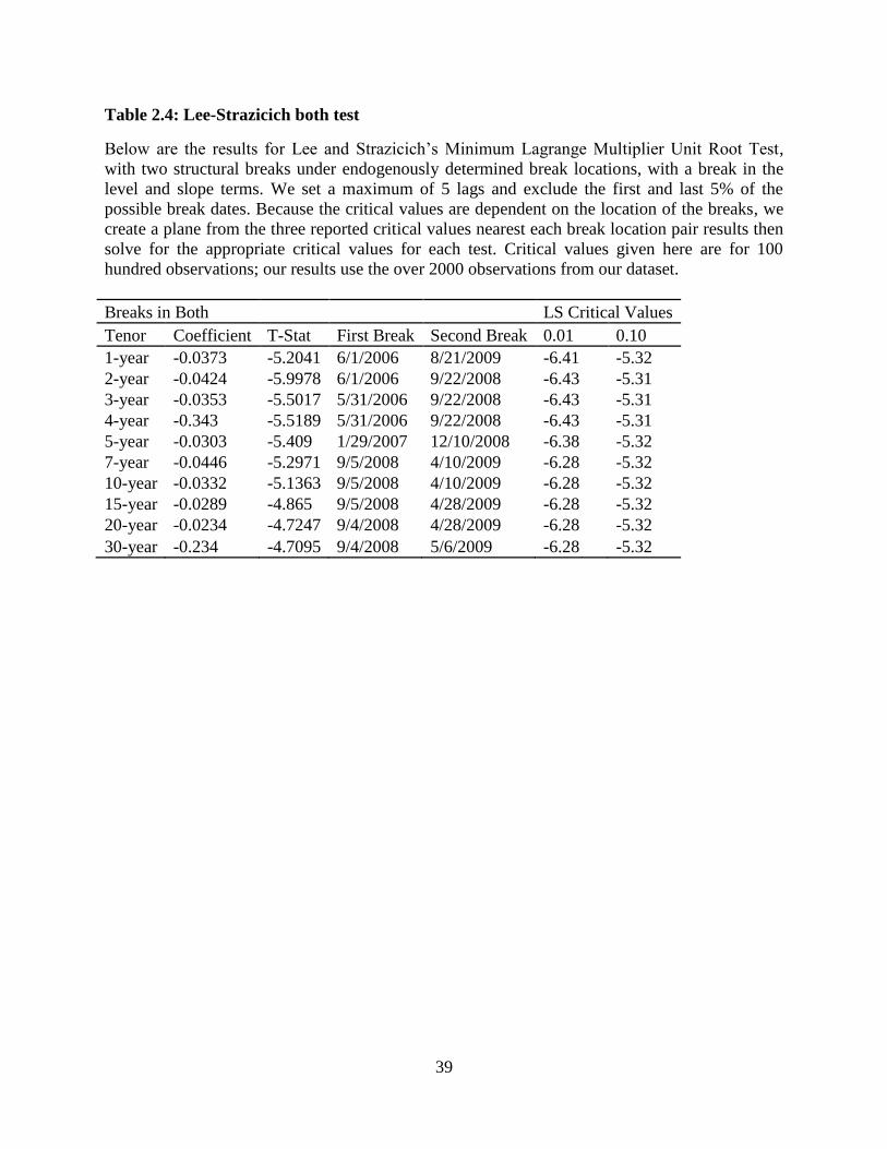
39
Table 2.4: Lee-Strazicich both test
Below are the results for Lee and Strazicich’s Minimum Lagrange Multiplier Unit Root Test,
with two structural breaks under endogenously determined break locations, with a break in the
level and slope terms. We set a maximum of 5 lags and exclude the first and last 5% of the
possible break dates. Because the critical values are dependent on the location of the breaks, we
create a plane from the three reported critical values nearest each break location pair results then
solve for the appropriate critical values for each test. Critical values given here are for 100
hundred observations; our results use the over 2000 observations from our dataset.
Breaks in Both LS Critical Values
Tenor Coefficient T-Stat First Break Second Break 0.01 0.10
1-year -0.0373 -5.2041 6/1/2006 8/21/2009 -6.41 -5.32
2-year -0.0424 -5.9978 6/1/2006 9/22/2008 -6.43 -5.31
3-year -0.0353 -5.5017 5/31/2006 9/22/2008 -6.43 -5.31
4-year -0.343 -5.5189 5/31/2006 9/22/2008 -6.43 -5.31
5-year -0.0303 -5.409 1/29/2007 12/10/2008 -6.38 -5.32
7-year -0.0446 -5.2971 9/5/2008 4/10/2009 -6.28 -5.32
10-year -0.0332 -5.1363 9/5/2008 4/10/2009 -6.28 -5.32
15-year -0.0289 -4.865 9/5/2008 4/28/2009 -6.28 -5.32
20-year -0.0234 -4.7247 9/4/2008 4/28/2009 -6.28 -5.32
30-year -0.234 -4.7095 9/4/2008 5/6/2009 -6.28 -5.32

40
Table 2.5: Error correction vector
The left side shows the linear regression of the error correction vector for the 1-year interest rate
swaps. The regression is done with ordinary least squares and variances are corrected for
heteroskedasticity and autocorrelation using White’s robust standard error from January 1, 2003
to March 3, 2011. This is the first part of the Engle-Granger Test for cointegration. The right side
shows the regression of the first difference of the residuals from the previous linear regression as
the dependent variable. The independent variable is the lagged residual. The null hypothesis of a
coefficient equal to zero means that there is not cointegration. We reject the null hypothesis in
favor of cointegration. ECV is defined as follows:
ln 𝑠𝑇;𝑡,𝑇 = 𝛾0̂ + 𝛾1̂ ln 𝑠𝑇𝐸;𝑡,𝑇 + 𝑒�̂�
Error Correction Vectors Cointegration Stat.
N-year Constant Ln(MSI) Coefficient T-statistic
1-year 0.1873 1.137 -0.0413 -6.762
Standard Error 0.0025 0.0025 0.0061
2-year 0.1743 1.1368 -0.031 -5.876
Standard Error 0.0023 0.0022 0.0053
3-year 0.1434 1.156 -0.0312 -5.842
Standard Error 0.0029 0.0028 0.0053
4-year 0.1032 1.1805 -0.0319 -5.883
Standard Error 0.0038 0.0035 0.0054
5-year 0.05 1.2148 -0.0278 -5.485
Standard Error 0.0048 0.0043 0.0051
7-year -0.0413 1.2709 -0.0857 -9.776
Standard Error 0.0075 0.0063 0.0088
10-year -0.1636 1.3424 -0.0291 -5.618
Standard Error 0.0095 0.0076 0.0052
15-year -0.3234 1.4284 -0.0261 -5.319
Standard Error 0.0137 0.0102 0.0049
20-year -0.3963 1.4605 -0.0214 -4.817
Standard Error 0.0156 0.0113 0.0044
30-year -0.5307 1.5353 -0.0241 -5.106
Standard Error 0.0174 0.0124 0.0047
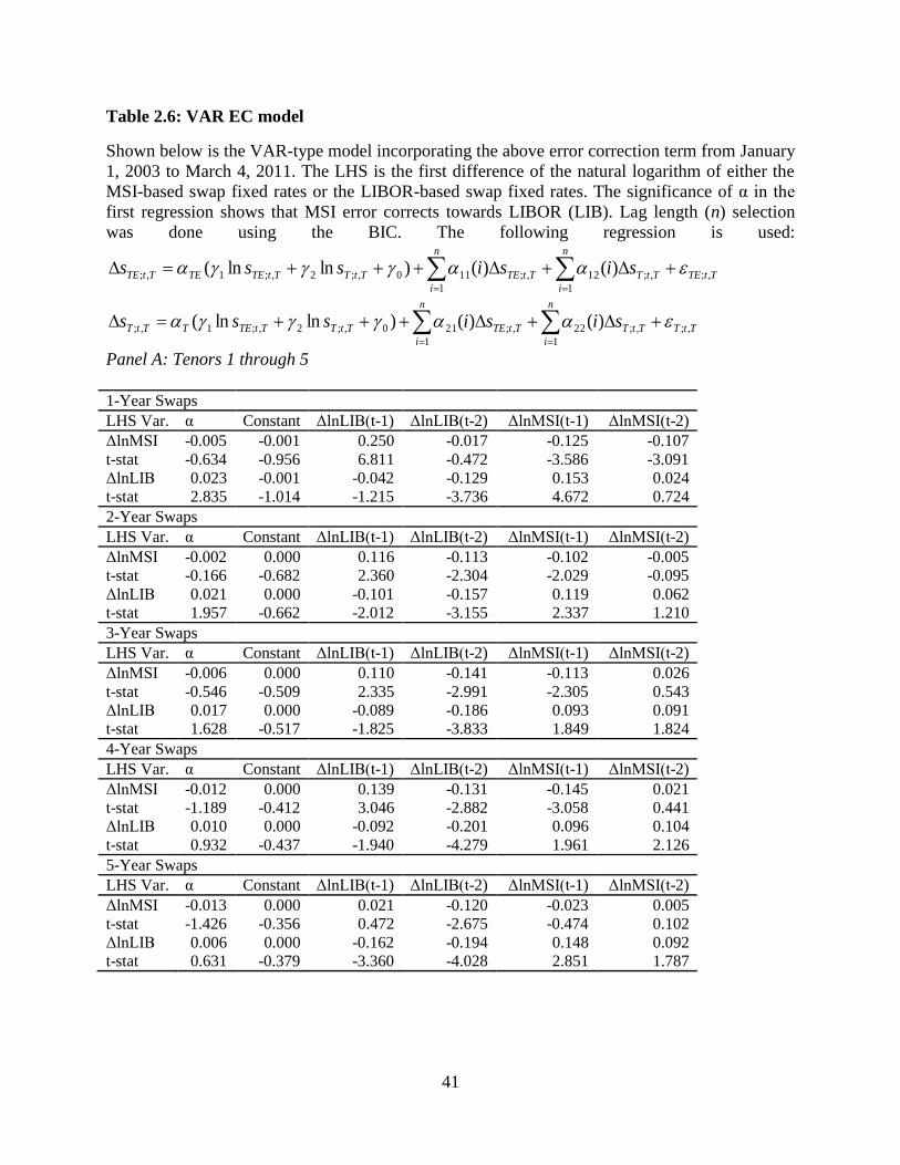
41
Table 2.6: VAR EC model
Shown below is the VAR-type model incorporating the above error correction term from January
1, 2003 to March 4, 2011. The LHS is the first difference of the natural logarithm of either the
MSI-based swap fixed rates or the LIBOR-based swap fixed rates. The significance of α in the
first regression shows that MSI error corrects towards LIBOR (LIB). Lag length (n) selection
was done using the BIC. The following regression is used:
TtTE
n
i
TtT
n
i
TtTETtTTtTETETtTE sisisss ,;
1
,;12
1
,;110,;2,;1,; )()()lnln(
TtT
n
i
TtT
n
i
TtTETtTTtTETTtT sisisss ,;
1
,;22
1
,;210,;2,;1,; )()()lnln(
Panel A: Tenors 1 through 5
1-Year Swaps
LHS Var. α Constant ΔlnLIB(t-1) ΔlnLIB(t-2) ΔlnMSI(t-1) ΔlnMSI(t-2)
ΔlnMSI -0.005 -0.001 0.250 -0.017 -0.125 -0.107
t-stat -0.634 -0.956 6.811 -0.472 -3.586 -3.091
ΔlnLIB 0.023 -0.001 -0.042 -0.129 0.153 0.024
t-stat 2.835 -1.014 -1.215 -3.736 4.672 0.724
2-Year Swaps
LHS Var. α Constant ΔlnLIB(t-1) ΔlnLIB(t-2) ΔlnMSI(t-1) ΔlnMSI(t-2)
ΔlnMSI -0.002 0.000 0.116 -0.113 -0.102 -0.005
t-stat -0.166 -0.682 2.360 -2.304 -2.029 -0.095
ΔlnLIB 0.021 0.000 -0.101 -0.157 0.119 0.062
t-stat 1.957 -0.662 -2.012 -3.155 2.337 1.210
3-Year Swaps
LHS Var. α Constant ΔlnLIB(t-1) ΔlnLIB(t-2) ΔlnMSI(t-1) ΔlnMSI(t-2)
ΔlnMSI -0.006 0.000 0.110 -0.141 -0.113 0.026
t-stat -0.546 -0.509 2.335 -2.991 -2.305 0.543
ΔlnLIB 0.017 0.000 -0.089 -0.186 0.093 0.091
t-stat 1.628 -0.517 -1.825 -3.833 1.849 1.824
4-Year Swaps
LHS Var. α Constant ΔlnLIB(t-1) ΔlnLIB(t-2) ΔlnMSI(t-1) ΔlnMSI(t-2)
ΔlnMSI -0.012 0.000 0.139 -0.131 -0.145 0.021
t-stat -1.189 -0.412 3.046 -2.882 -3.058 0.441
ΔlnLIB 0.010 0.000 -0.092 -0.201 0.096 0.104
t-stat 0.932 -0.437 -1.940 -4.279 1.961 2.126
5-Year Swaps
LHS Var. α Constant ΔlnLIB(t-1) ΔlnLIB(t-2) ΔlnMSI(t-1) ΔlnMSI(t-2)
ΔlnMSI -0.013 0.000 0.021 -0.120 -0.023 0.005
t-stat -1.426 -0.356 0.472 -2.675 -0.474 0.102
ΔlnLIB 0.006 0.000 -0.162 -0.194 0.148 0.092
t-stat 0.631 -0.379 -3.360 -4.028 2.851 1.787
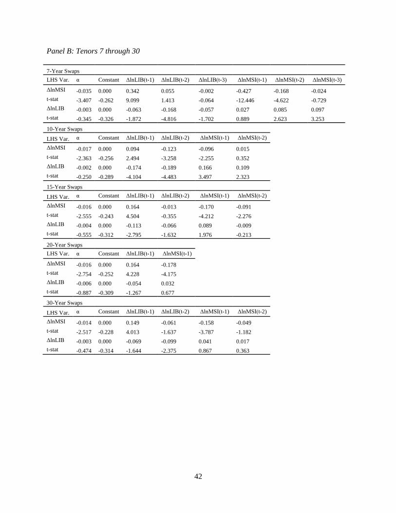
42
Panel B: Tenors 7 through 30
7-Year Swaps
LHS Var. α Constant ΔlnLIB(t-1) ΔlnLIB(t-2) ΔlnLIB(t-3) ΔlnMSI(t-1) ΔlnMSI(t-2) ΔlnMSI(t-3)
ΔlnMSI -0.035 0.000 0.342 0.055 -0.002 -0.427 -0.168 -0.024
t-stat -3.407 -0.262 9.099 1.413 -0.064 -12.446 -4.622 -0.729
ΔlnLIB -0.003 0.000 -0.063 -0.168 -0.057 0.027 0.085 0.097
t-stat -0.345 -0.326 -1.872 -4.816 -1.702 0.889 2.623 3.253
10-Year Swaps
LHS Var. α Constant ΔlnLIB(t-1) ΔlnLIB(t-2) ΔlnMSI(t-1) ΔlnMSI(t-2)
ΔlnMSI -0.017 0.000 0.094 -0.123 -0.096 0.015
t-stat -2.363 -0.256 2.494 -3.258 -2.255 0.352
ΔlnLIB -0.002 0.000 -0.174 -0.189 0.166 0.109
t-stat -0.250 -0.289 -4.104 -4.483 3.497 2.323
15-Year Swaps
LHS Var. α Constant ΔlnLIB(t-1) ΔlnLIB(t-2) ΔlnMSI(t-1) ΔlnMSI(t-2)
ΔlnMSI -0.016 0.000 0.164 -0.013 -0.170 -0.091
t-stat -2.555 -0.243 4.504 -0.355 -4.212 -2.276
ΔlnLIB -0.004 0.000 -0.113 -0.066 0.089 -0.009
t-stat -0.555 -0.312 -2.795 -1.632 1.976 -0.213
20-Year Swaps
LHS Var. α Constant ΔlnLIB(t-1) ΔlnMSI(t-1)
ΔlnMSI -0.016 0.000 0.164 -0.178
t-stat -2.754 -0.252 4.228 -4.175
ΔlnLIB -0.006 0.000 -0.054 0.032
t-stat -0.887 -0.309 -1.267 0.677
30-Year Swaps
LHS Var. α Constant ΔlnLIB(t-1) ΔlnLIB(t-2) ΔlnMSI(t-1) ΔlnMSI(t-2)
ΔlnMSI -0.014 0.000 0.149 -0.061 -0.158 -0.049
t-stat -2.517 -0.228 4.013 -1.637 -3.787 -1.182
ΔlnLIB -0.003 0.000 -0.069 -0.099 0.041 0.017
t-stat -0.474 -0.314 -1.644 -2.375 0.867 0.363
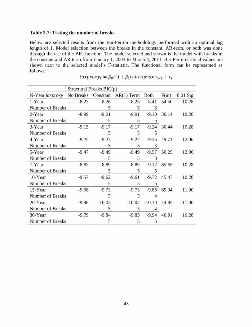
43
Table 2.7: Testing the number of breaks
Below are selected results from the Bai-Perron methodology performed with an optimal lag
length of 1. Model selection between the breaks in the constant, AR-term, or both was done
through the use of the BIC function. The model selected and shown is the model with breaks in
the constant and AR term from January 1, 2003 to March 4, 2011. Bai-Perron critical values are
shown next to the selected model’s F-statistic. The functional form can be represented as
follows:
𝑡𝑎𝑥𝑝𝑟𝑜𝑥𝑦𝑡 = 𝛽0(𝑡) + 𝛽1(𝑡)𝑡𝑎𝑥𝑝𝑟𝑜𝑥𝑦𝑡−1 + 휀𝑡
Structural Breaks BIC(p)
N-Year taxproxy No Breaks Constant AR(1) Term Both F(m) 0.01 Sig
1-Year -8.23 -8.26 -8.25 -8.41 54.50 10.28
Number of Breaks 5 5 5
2-Year -8.99 -9.01 -9.01 -9.10 36.14 10.28
Number of Breaks 5 5 5
3-Year -9.15 -9.17 -9.17 -9.24 30.44 10.28
Number of Breaks 5 5 5
4-Year -9.25 -9.27 -9.27 -9.35 49.71 12.06
Number of Breaks 5 5 3
5-Year -9.47 -9.49 -9.49 -9.57 50.25 12.06
Number of Breaks 5 5 3
7-Year -8.83 -8.89 -8.89 -9.12 85.65 10.28
Number of Breaks 5 5 5
10-Year -9.57 -9.62 -9.61 -9.72 45.47 10.28
Number of Breaks 5 5 5
15-Year -9.68 -9.73 -9.73 -9.86 65.04 11.00
Number of Breaks 5 5 4
20-Year -9.98 -10.03 -10.02 -10.10 44.95 11.00
Number of Breaks 5 5 4
30-Year -9.79 -9.84 -9.83 -9.94 46.91 10.28
Number of Breaks 5 5 5
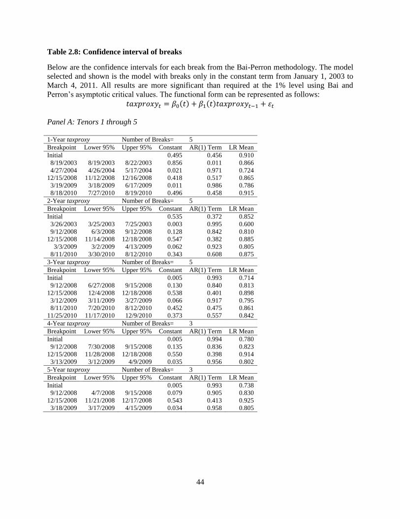
44
Table 2.8: Confidence interval of breaks
Below are the confidence intervals for each break from the Bai-Perron methodology. The model
selected and shown is the model with breaks only in the constant term from January 1, 2003 to
March 4, 2011. All results are more significant than required at the 1% level using Bai and
Perron’s asymptotic critical values. The functional form can be represented as follows:
𝑡𝑎𝑥𝑝𝑟𝑜𝑥𝑦𝑡 = 𝛽0(𝑡) + 𝛽1(𝑡)𝑡𝑎𝑥𝑝𝑟𝑜𝑥𝑦𝑡−1 + 휀𝑡
Panel A: Tenors 1 through 5
1-Year taxproxy Number of Breaks= 5
Breakpoint Lower 95% Upper 95% Constant AR(1) Term LR Mean
Initial
0.495 0.456 0.910
8/19/2003 8/19/2003 8/22/2003 0.856 0.011 0.866
4/27/2004 4/26/2004 5/17/2004 0.021 0.971 0.724
12/15/2008 11/12/2008 12/16/2008 0.418 0.517 0.865
3/19/2009 3/18/2009 6/17/2009 0.011 0.986 0.786
8/18/2010 7/27/2010 8/19/2010 0.496 0.458 0.915
2-Year taxproxy Number of Breaks= 5
Breakpoint Lower 95% Upper 95% Constant AR(1) Term LR Mean
Initial
0.535 0.372 0.852
3/26/2003 3/25/2003 7/25/2003 0.003 0.995 0.600
9/12/2008 6/3/2008 9/12/2008 0.128 0.842 0.810
12/15/2008 11/14/2008 12/18/2008 0.547 0.382 0.885
3/3/2009 3/2/2009 4/13/2009 0.062 0.923 0.805
8/11/2010 3/30/2010 8/12/2010 0.343 0.608 0.875
3-Year taxproxy Number of Breaks= 5
Breakpoint Lower 95% Upper 95% Constant AR(1) Term LR Mean
Initial
0.005 0.993 0.714
9/12/2008 6/27/2008 9/15/2008 0.130 0.840 0.813
12/15/2008 12/4/2008 12/18/2008 0.538 0.401 0.898
3/12/2009 3/11/2009 3/27/2009 0.066 0.917 0.795
8/11/2010 7/20/2010 8/12/2010 0.452 0.475 0.861
11/25/2010 11/17/2010 12/9/2010 0.373 0.557 0.842
4-Year taxproxy Number of Breaks= 3
Breakpoint Lower 95% Upper 95% Constant AR(1) Term LR Mean
Initial
0.005 0.994 0.780
9/12/2008 7/30/2008 9/15/2008 0.135 0.836 0.823
12/15/2008 11/28/2008 12/18/2008 0.550 0.398 0.914
3/13/2009 3/12/2009 4/9/2009 0.035 0.956 0.802
5-Year taxproxy Number of Breaks= 3
Breakpoint Lower 95% Upper 95% Constant AR(1) Term LR Mean
Initial
0.005 0.993 0.738
9/12/2008 4/7/2008 9/15/2008 0.079 0.905 0.830
12/15/2008 11/21/2008 12/17/2008 0.543 0.413 0.925
3/18/2009 3/17/2009 4/15/2009 0.034 0.958 0.805
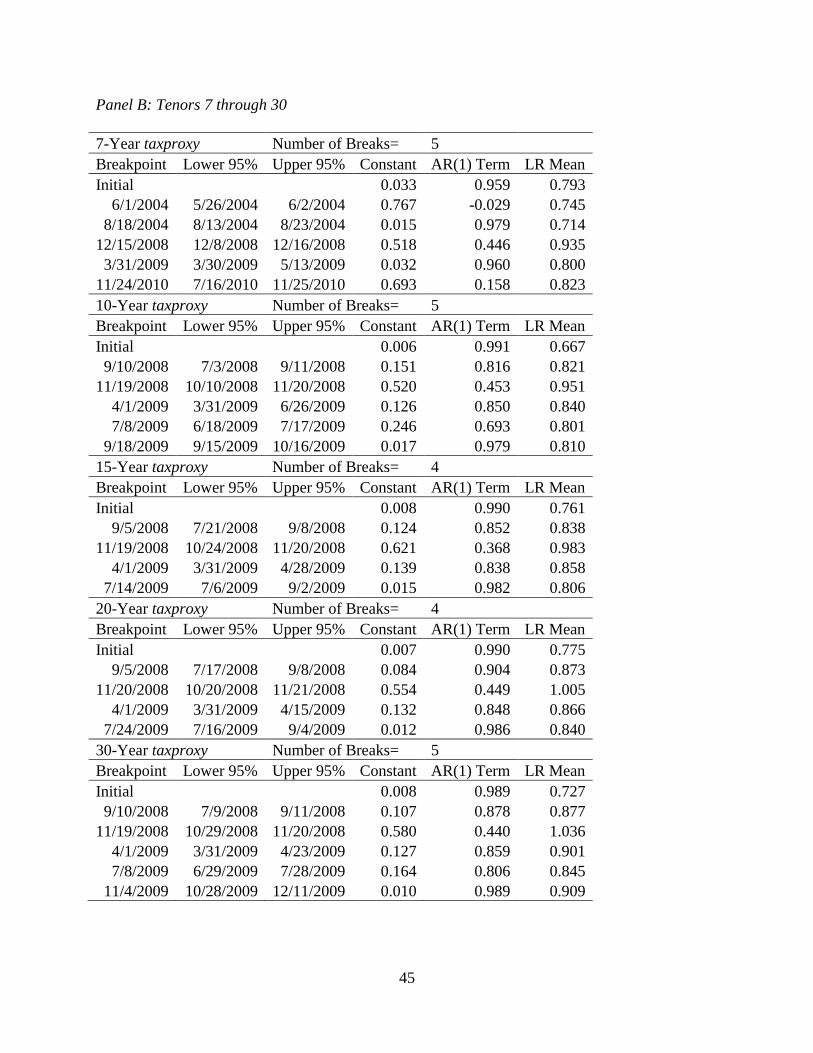
45
Panel B: Tenors 7 through 30
7-Year taxproxy Number of Breaks= 5
Breakpoint Lower 95% Upper 95% Constant AR(1) Term LR Mean
Initial
0.033 0.959 0.793
6/1/2004 5/26/2004 6/2/2004 0.767 -0.029 0.745
8/18/2004 8/13/2004 8/23/2004 0.015 0.979 0.714
12/15/2008 12/8/2008 12/16/2008 0.518 0.446 0.935
3/31/2009 3/30/2009 5/13/2009 0.032 0.960 0.800
11/24/2010 7/16/2010 11/25/2010 0.693 0.158 0.823
10-Year taxproxy Number of Breaks= 5
Breakpoint Lower 95% Upper 95% Constant AR(1) Term LR Mean
Initial
0.006 0.991 0.667
9/10/2008 7/3/2008 9/11/2008 0.151 0.816 0.821
11/19/2008 10/10/2008 11/20/2008 0.520 0.453 0.951
4/1/2009 3/31/2009 6/26/2009 0.126 0.850 0.840
7/8/2009 6/18/2009 7/17/2009 0.246 0.693 0.801
9/18/2009 9/15/2009 10/16/2009 0.017 0.979 0.810
15-Year taxproxy Number of Breaks= 4
Breakpoint Lower 95% Upper 95% Constant AR(1) Term LR Mean
Initial
0.008 0.990 0.761
9/5/2008 7/21/2008 9/8/2008 0.124 0.852 0.838
11/19/2008 10/24/2008 11/20/2008 0.621 0.368 0.983
4/1/2009 3/31/2009 4/28/2009 0.139 0.838 0.858
7/14/2009 7/6/2009 9/2/2009 0.015 0.982 0.806
20-Year taxproxy Number of Breaks= 4
Breakpoint Lower 95% Upper 95% Constant AR(1) Term LR Mean
Initial
0.007 0.990 0.775
9/5/2008 7/17/2008 9/8/2008 0.084 0.904 0.873
11/20/2008 10/20/2008 11/21/2008 0.554 0.449 1.005
4/1/2009 3/31/2009 4/15/2009 0.132 0.848 0.866
7/24/2009 7/16/2009 9/4/2009 0.012 0.986 0.840
30-Year taxproxy Number of Breaks= 5
Breakpoint Lower 95% Upper 95% Constant AR(1) Term LR Mean
Initial
0.008 0.989 0.727
9/10/2008 7/9/2008 9/11/2008 0.107 0.878 0.877
11/19/2008 10/29/2008 11/20/2008 0.580 0.440 1.036
4/1/2009 3/31/2009 4/23/2009 0.127 0.859 0.901
7/8/2009 6/29/2009 7/28/2009 0.164 0.806 0.845
11/4/2009 10/28/2009 12/11/2009 0.010 0.989 0.909
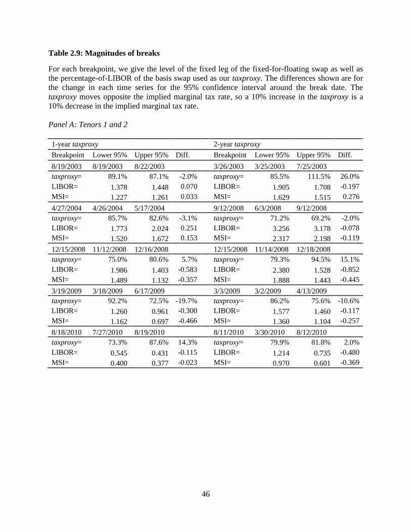
46
Table 2.9: Magnitudes of breaks
For each breakpoint, we give the level of the fixed leg of the fixed-for-floating swap as well as
the percentage-of-LIBOR of the basis swap used as our taxproxy. The differences shown are for
the change in each time series for the 95% confidence interval around the break date. The
taxproxy moves opposite the implied marginal tax rate, so a 10% increase in the taxproxy is a
10% decrease in the implied marginal tax rate.
Panel A: Tenors 1 and 2
1-year taxproxy 2-year taxproxy
Breakpoint Lower 95% Upper 95% Diff. Breakpoint Lower 95% Upper 95% Diff.
8/19/2003 8/19/2003 8/22/2003 3/26/2003 3/25/2003 7/25/2003
taxproxy= 89.1% 87.1% -2.0%
taxproxy= 85.5% 111.5% 26.0%
LIBOR= 1.378 1.448 0.070
LIBOR= 1.905 1.708 -0.197
MSI= 1.227 1.261 0.033
MSI= 1.629 1.515 0.276
4/27/2004 4/26/2004 5/17/2004 9/12/2008 6/3/2008 9/12/2008
taxproxy= 85.7% 82.6% -3.1%
taxproxy= 71.2% 69.2% -2.0%
LIBOR= 1.773 2.024 0.251
LIBOR= 3.256 3.178 -0.078
MSI= 1.520 1.672 0.153
MSI= 2.317 2.198 -0.119
12/15/2008 11/12/2008 12/16/2008 12/15/2008 11/14/2008 12/18/2008
taxproxy= 75.0% 80.6% 5.7%
taxproxy= 79.3% 94.5% 15.1%
LIBOR= 1.986 1.403 -0.583
LIBOR= 2.380 1.528 -0.852
MSI= 1.489 1.132 -0.357
MSI= 1.888 1.443 -0.445
3/19/2009 3/18/2009 6/17/2009 3/3/2009 3/2/2009 4/13/2009
taxproxy= 92.2% 72.5% -19.7%
taxproxy= 86.2% 75.6% -10.6%
LIBOR= 1.260 0.961 -0.300
LIBOR= 1.577 1.460 -0.117
MSI= 1.162 0.697 -0.466
MSI= 1.360 1.104 -0.257
8/18/2010 7/27/2010 8/19/2010 8/11/2010 3/30/2010 8/12/2010
taxproxy= 73.3% 87.6% 14.3%
taxproxy= 79.9% 81.8% 2.0%
LIBOR= 0.545 0.431 -0.115
LIBOR= 1.214 0.735 -0.480
MSI= 0.400 0.377 -0.023 MSI= 0.970 0.601 -0.369
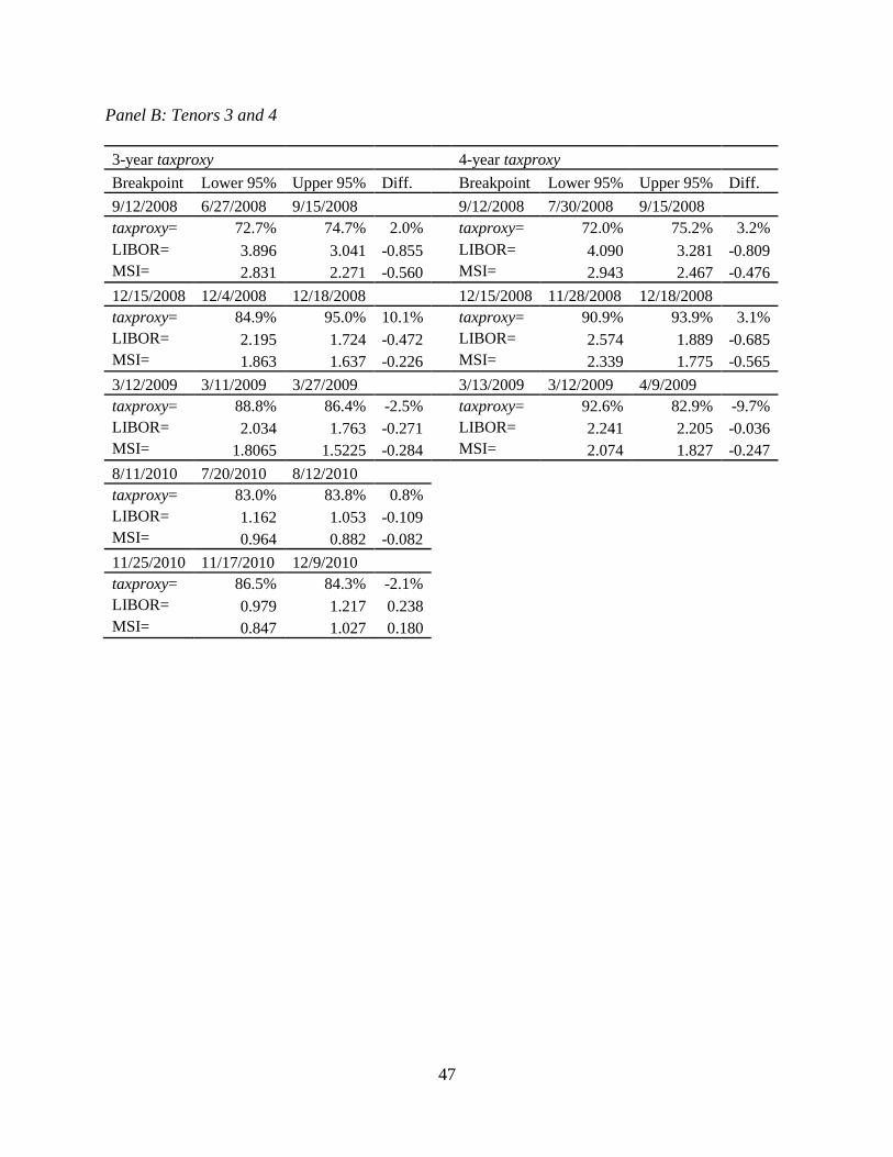
47
Panel B: Tenors 3 and 4
3-year taxproxy 4-year taxproxy
Breakpoint Lower 95% Upper 95% Diff. Breakpoint Lower 95% Upper 95% Diff.
9/12/2008 6/27/2008 9/15/2008 9/12/2008 7/30/2008 9/15/2008
taxproxy= 72.7% 74.7% 2.0%
taxproxy= 72.0% 75.2% 3.2%
LIBOR= 3.896 3.041 -0.855
LIBOR= 4.090 3.281 -0.809
MSI= 2.831 2.271 -0.560
MSI= 2.943 2.467 -0.476
12/15/2008 12/4/2008 12/18/2008 12/15/2008 11/28/2008 12/18/2008
taxproxy= 84.9% 95.0% 10.1%
taxproxy= 90.9% 93.9% 3.1%
LIBOR= 2.195 1.724 -0.472
LIBOR= 2.574 1.889 -0.685
MSI= 1.863 1.637 -0.226
MSI= 2.339 1.775 -0.565
3/12/2009 3/11/2009 3/27/2009 3/13/2009 3/12/2009 4/9/2009
taxproxy= 88.8% 86.4% -2.5%
taxproxy= 92.6% 82.9% -9.7%
LIBOR= 2.034 1.763 -0.271
LIBOR= 2.241 2.205 -0.036
MSI= 1.8065 1.5225 -0.284 MSI= 2.074 1.827 -0.247
8/11/2010 7/20/2010 8/12/2010
taxproxy= 83.0% 83.8% 0.8%
LIBOR= 1.162 1.053 -0.109
MSI= 0.964 0.882 -0.082
11/25/2010 11/17/2010 12/9/2010
taxproxy= 86.5% 84.3% -2.1%
LIBOR= 0.979 1.217 0.238
MSI= 0.847 1.027 0.180
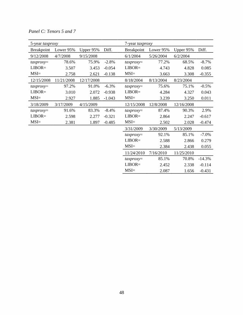
48
Panel C: Tenors 5 and 7
5-year taxproxy 7-year taxproxy
Breakpoint Lower 95% Upper 95% Diff. Breakpoint Lower 95% Upper 95% Diff.
9/12/2008 4/7/2008 9/15/2008 6/1/2004 5/26/2004 6/2/2004
taxproxy= 78.6% 75.9% -2.8%
taxproxy= 77.2% 68.5% -8.7%
LIBOR= 3.507 3.453 -0.054
LIBOR= 4.743 4.828 0.085
MSI= 2.758 2.621 -0.138
MSI= 3.663 3.308 -0.355
12/15/2008 11/21/2008 12/17/2008 8/18/2004 8/13/2004 8/23/2004
taxproxy= 97.2% 91.0% -6.3%
taxproxy= 75.6% 75.1% -0.5%
LIBOR= 3.010 2.072 -0.938
LIBOR= 4.284 4.327 0.043
MSI= 2.927 1.885 -1.043
MSI= 3.239 3.250 0.011
3/18/2009 3/17/2009 4/15/2009 12/15/2008 12/8/2008 12/16/2008
taxproxy= 91.6% 83.3% -8.4%
taxproxy= 87.4% 90.3% 2.9%
LIBOR= 2.598 2.277 -0.321
LIBOR= 2.864 2.247 -0.617
MSI= 2.381 1.897 -0.485 MSI= 2.502 2.028 -0.474
3/31/2009 3/30/2009 5/13/2009
taxproxy= 92.1% 85.1% -7.0%
LIBOR= 2.588 2.866 0.279
MSI= 2.384 2.438 0.055
11/24/2010 7/16/2010 11/25/2010
taxproxy= 85.1% 70.8% -14.3%
LIBOR= 2.452 2.338 -0.114
MSI= 2.087 1.656 -0.431
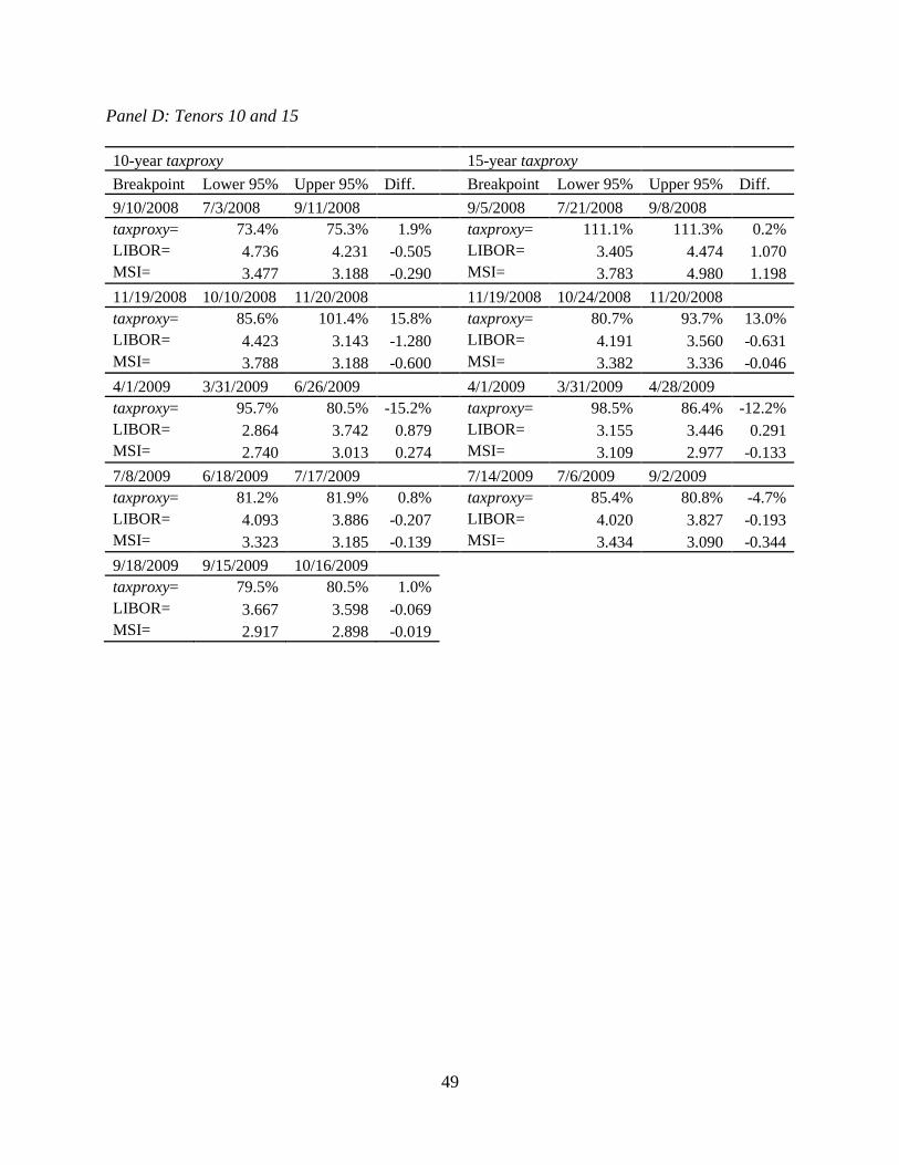
49
Panel D: Tenors 10 and 15
10-year taxproxy 15-year taxproxy
Breakpoint Lower 95% Upper 95% Diff. Breakpoint Lower 95% Upper 95% Diff.
9/10/2008 7/3/2008 9/11/2008 9/5/2008 7/21/2008 9/8/2008
taxproxy= 73.4% 75.3% 1.9%
taxproxy= 111.1% 111.3% 0.2%
LIBOR= 4.736 4.231 -0.505
LIBOR= 3.405 4.474 1.070
MSI= 3.477 3.188 -0.290
MSI= 3.783 4.980 1.198
11/19/2008 10/10/2008 11/20/2008 11/19/2008 10/24/2008 11/20/2008
taxproxy= 85.6% 101.4% 15.8%
taxproxy= 80.7% 93.7% 13.0%
LIBOR= 4.423 3.143 -1.280
LIBOR= 4.191 3.560 -0.631
MSI= 3.788 3.188 -0.600
MSI= 3.382 3.336 -0.046
4/1/2009 3/31/2009 6/26/2009 4/1/2009 3/31/2009 4/28/2009
taxproxy= 95.7% 80.5% -15.2%
taxproxy= 98.5% 86.4% -12.2%
LIBOR= 2.864 3.742 0.879
LIBOR= 3.155 3.446 0.291
MSI= 2.740 3.013 0.274
MSI= 3.109 2.977 -0.133
7/8/2009 6/18/2009 7/17/2009 7/14/2009 7/6/2009 9/2/2009
taxproxy= 81.2% 81.9% 0.8%
taxproxy= 85.4% 80.8% -4.7%
LIBOR= 4.093 3.886 -0.207
LIBOR= 4.020 3.827 -0.193
MSI= 3.323 3.185 -0.139 MSI= 3.434 3.090 -0.344
9/18/2009 9/15/2009 10/16/2009
taxproxy= 79.5% 80.5% 1.0%
LIBOR= 3.667 3.598 -0.069
MSI= 2.917 2.898 -0.019
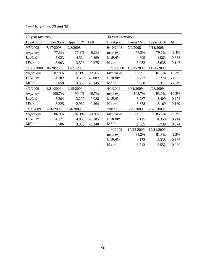
50
Panel E: Tenors 20 and 30
20-year taxproxy 30-year taxproxy
Breakpoint Lower 95% Upper 95% Diff. Breakpoint Lower 95% Upper 95% Diff.
9/5/2008 7/17/2008 9/8/2008 9/10/2008 7/9/2008 9/11/2008
taxproxy= 77.5% 77.3% -0.2%
taxproxy= 77.3% 79.7% 2.4%
LIBOR= 5.033 4.564 -0.469
LIBOR= 4.895 4.563 -0.332
MSI= 3.903 3.528 -0.375
MSI= 3.782 3.635 -0.147
11/20/2008 10/20/2008 11/21/2008 11/19/2008 10/29/2008 11/20/2008
taxproxy= 87.8% 100.1% 12.3%
taxproxy= 85.7% 101.0% 15.3%
LIBOR= 4.382 3.500 -0.882
LIBOR= 4.272 3.278 -0.995
MSI= 3.850 3.505 -0.345
MSI= 3.660 3.311 -0.349
4/1/2009 3/31/2009 4/15/2009 4/1/2009 3/31/2009 4/23/2009
taxproxy= 100.7% 90.0% -10.7%
taxproxy= 103.7% 93.0% -10.8%
LIBOR= 3.204 3.292 0.088
LIBOR= 3.237 3.409 0.172
MSI= 3.225 2.962 -0.264
MSI= 3.358 3.169 -0.189
7/24/2009 7/16/2009 9/4/2009 7/8/2009 6/29/2009 7/28/2009
taxproxy= 86.0% 82.1% -3.9%
taxproxy= 89.1% 85.8% -3.3%
LIBOR= 4.171 4.066 -0.105
LIBOR= 4.115 4.359 0.244
MSI= 3.586 3.338 -0.248 MSI= 3.665 3.739 0.074
11/4/2009 10/28/2009 12/11/2009
taxproxy= 84.2% 81.9% -2.3%
LIBOR= 4.172 4.338 0.166
MSI= 3.513 3.552 0.039
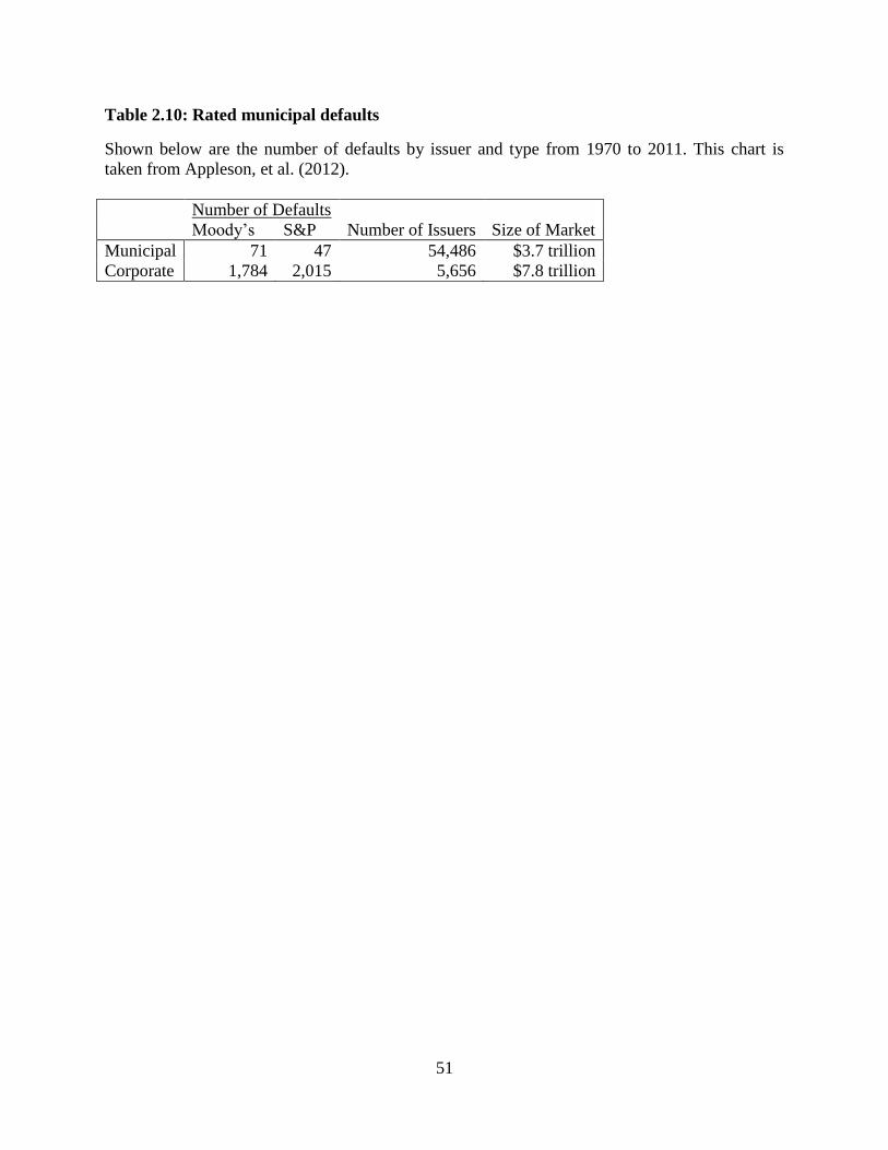
51
Table 2.10: Rated municipal defaults
Shown below are the number of defaults by issuer and type from 1970 to 2011. This chart is
taken from Appleson, et al. (2012).
Number of Defaults
Moody’s S&P Number of Issuers Size of Market
Municipal 71 47 54,486 $3.7 trillion
Corporate 1,784 2,015 5,656 $7.8 trillion
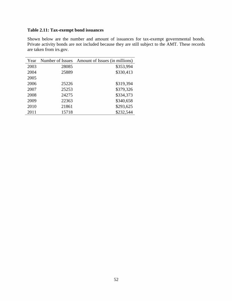
52
Table 2.11: Tax-exempt bond issuances
Shown below are the number and amount of issuances for tax-exempt governmental bonds.
Private activity bonds are not included because they are still subject to the AMT. These records
are taken from irs.gov.
Year Number of Issues Amount of Issues (in millions)
2003 28085 $353,994
2004 25889 $330,413
2005
2006 25226 $319,394
2007 25253 $379,326
2008 24275 $334,373
2009 22363 $340,658
2010 21861 $293,625
2011 15718 $232,544
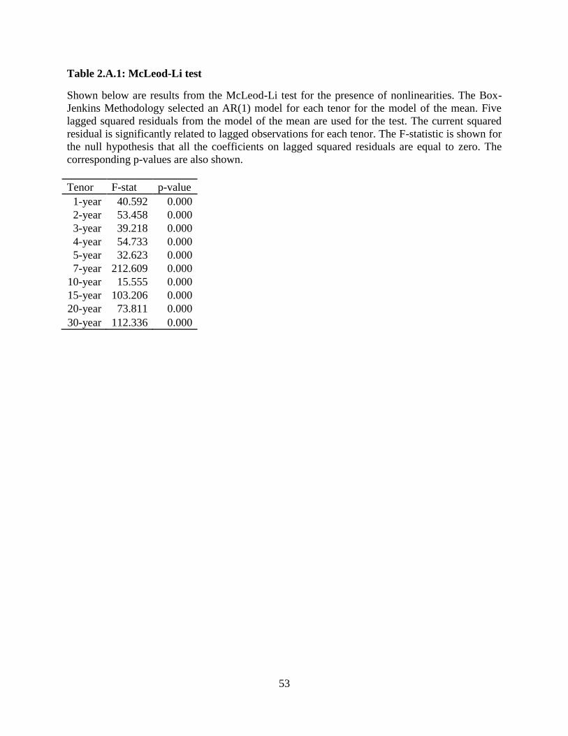
53
Table 2.A.1: McLeod-Li test
Shown below are results from the McLeod-Li test for the presence of nonlinearities. The Box-
Jenkins Methodology selected an AR(1) model for each tenor for the model of the mean. Five
lagged squared residuals from the model of the mean are used for the test. The current squared
residual is significantly related to lagged observations for each tenor. The F-statistic is shown for
the null hypothesis that all the coefficients on lagged squared residuals are equal to zero. The
corresponding p-values are also shown.
Tenor F-stat p-value
1-year 40.592 0.000
2-year 53.458 0.000
3-year 39.218 0.000
4-year 54.733 0.000
5-year 32.623 0.000
7-year 212.609 0.000
10-year 15.555 0.000
15-year 103.206 0.000
20-year 73.811 0.000
30-year 112.336 0.000
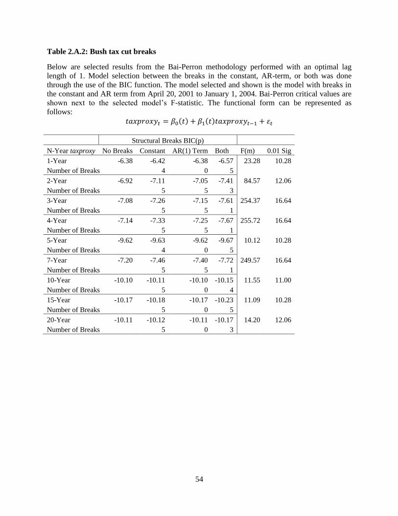
54
Table 2.A.2: Bush tax cut breaks
Below are selected results from the Bai-Perron methodology performed with an optimal lag
length of 1. Model selection between the breaks in the constant, AR-term, or both was done
through the use of the BIC function. The model selected and shown is the model with breaks in
the constant and AR term from April 20, 2001 to January 1, 2004. Bai-Perron critical values are
shown next to the selected model’s F-statistic. The functional form can be represented as
follows:
𝑡𝑎𝑥𝑝𝑟𝑜𝑥𝑦𝑡 = 𝛽0(𝑡) + 𝛽1(𝑡)𝑡𝑎𝑥𝑝𝑟𝑜𝑥𝑦𝑡−1 + 휀𝑡
Structural Breaks BIC(p)
N-Year taxproxy No Breaks Constant AR(1) Term Both F(m) 0.01 Sig
1-Year -6.38 -6.42 -6.38 -6.57 23.28 10.28
Number of Breaks 4 0 5
2-Year -6.92 -7.11 -7.05 -7.41 84.57 12.06
Number of Breaks 5 5 3
3-Year -7.08 -7.26 -7.15 -7.61 254.37 16.64
Number of Breaks 5 5 1
4-Year -7.14 -7.33 -7.25 -7.67 255.72 16.64
Number of Breaks 5 5 1
5-Year -9.62 -9.63 -9.62 -9.67 10.12 10.28
Number of Breaks 4 0 5
7-Year -7.20 -7.46 -7.40 -7.72 249.57 16.64
Number of Breaks 5 5 1
10-Year -10.10 -10.11 -10.10 -10.15 11.55 11.00
Number of Breaks 5 0 4
15-Year -10.17 -10.18 -10.17 -10.23 11.09 10.28
Number of Breaks 5 0 5
20-Year -10.11 -10.12 -10.11 -10.17 14.20 12.06
Number of Breaks 5 0 3
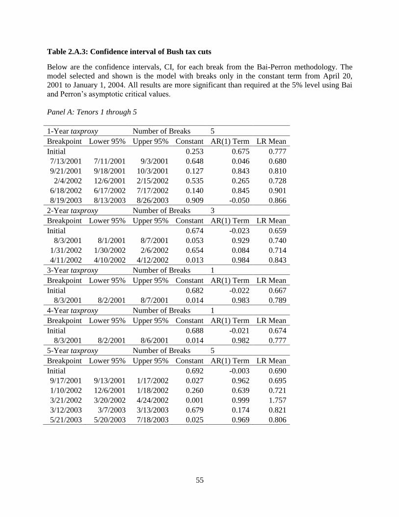
55
Table 2.A.3: Confidence interval of Bush tax cuts
Below are the confidence intervals, CI, for each break from the Bai-Perron methodology. The
model selected and shown is the model with breaks only in the constant term from April 20,
2001 to January 1, 2004. All results are more significant than required at the 5% level using Bai
and Perron’s asymptotic critical values.
Panel A: Tenors 1 through 5
1-Year taxproxy Number of Breaks 5
Breakpoint Lower 95% Upper 95% Constant AR(1) Term LR Mean
Initial
0.253 0.675 0.777
7/13/2001 7/11/2001 9/3/2001 0.648 0.046 0.680
9/21/2001 9/18/2001 10/3/2001 0.127 0.843 0.810
2/4/2002 12/6/2001 2/15/2002 0.535 0.265 0.728
6/18/2002 6/17/2002 7/17/2002 0.140 0.845 0.901
8/19/2003 8/13/2003 8/26/2003 0.909 -0.050 0.866
2-Year taxproxy Number of Breaks 3
Breakpoint Lower 95% Upper 95% Constant AR(1) Term LR Mean
Initial
0.674 -0.023 0.659
8/3/2001 8/1/2001 8/7/2001 0.053 0.929 0.740
1/31/2002 1/30/2002 2/6/2002 0.654 0.084 0.714
4/11/2002 4/10/2002 4/12/2002 0.013 0.984 0.843
3-Year taxproxy Number of Breaks 1
Breakpoint Lower 95% Upper 95% Constant AR(1) Term LR Mean
Initial
0.682 -0.022 0.667
8/3/2001 8/2/2001 8/7/2001 0.014 0.983 0.789
4-Year taxproxy Number of Breaks 1
Breakpoint Lower 95% Upper 95% Constant AR(1) Term LR Mean
Initial
0.688 -0.021 0.674
8/3/2001 8/2/2001 8/6/2001 0.014 0.982 0.777
5-Year taxproxy Number of Breaks 5
Breakpoint Lower 95% Upper 95% Constant AR(1) Term LR Mean
Initial
0.692 -0.003 0.690
9/17/2001 9/13/2001 1/17/2002 0.027 0.962 0.695
1/10/2002 12/6/2001 1/18/2002 0.260 0.639 0.721
3/21/2002 3/20/2002 4/24/2002 0.001 0.999 1.757
3/12/2003 3/7/2003 3/13/2003 0.679 0.174 0.821
5/21/2003 5/20/2003 7/18/2003 0.025 0.969 0.806
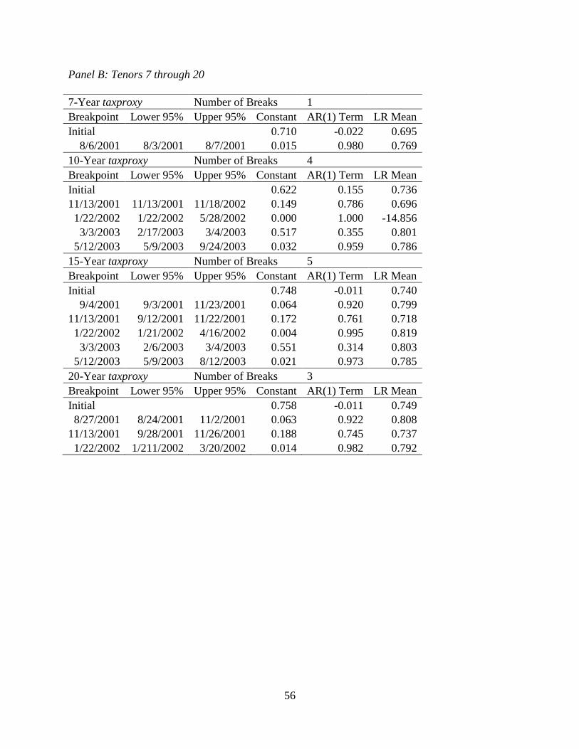
56
Panel B: Tenors 7 through 20
7-Year taxproxy Number of Breaks 1
Breakpoint Lower 95% Upper 95% Constant AR(1) Term LR Mean
Initial
0.710 -0.022 0.695
8/6/2001 8/3/2001 8/7/2001 0.015 0.980 0.769
10-Year taxproxy Number of Breaks 4
Breakpoint Lower 95% Upper 95% Constant AR(1) Term LR Mean
Initial
0.622 0.155 0.736
11/13/2001 11/13/2001 11/18/2002 0.149 0.786 0.696
1/22/2002 1/22/2002 5/28/2002 0.000 1.000 -14.856
3/3/2003 2/17/2003 3/4/2003 0.517 0.355 0.801
5/12/2003 5/9/2003 9/24/2003 0.032 0.959 0.786
15-Year taxproxy Number of Breaks 5
Breakpoint Lower 95% Upper 95% Constant AR(1) Term LR Mean
Initial
0.748 -0.011 0.740
9/4/2001 9/3/2001 11/23/2001 0.064 0.920 0.799
11/13/2001 9/12/2001 11/22/2001 0.172 0.761 0.718
1/22/2002 1/21/2002 4/16/2002 0.004 0.995 0.819
3/3/2003 2/6/2003 3/4/2003 0.551 0.314 0.803
5/12/2003 5/9/2003 8/12/2003 0.021 0.973 0.785
20-Year taxproxy Number of Breaks 3
Breakpoint Lower 95% Upper 95% Constant AR(1) Term LR Mean
Initial
0.758 -0.011 0.749
8/27/2001 8/24/2001 11/2/2001 0.063 0.922 0.808
11/13/2001 9/28/2001 11/26/2001 0.188 0.745 0.737
1/22/2002 1/211/2002 3/20/2002 0.014 0.982 0.792
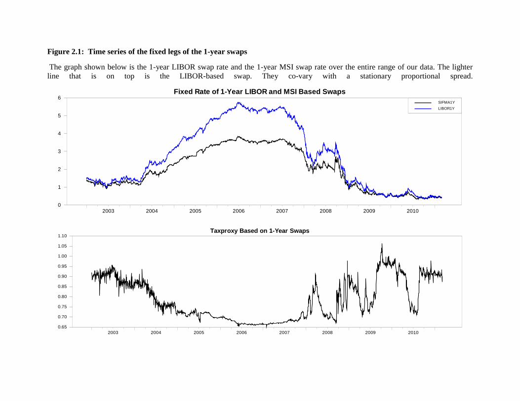
Figure 2.1: Time series of the fixed legs of the 1-year swaps
The graph shown below is the 1-year LIBOR swap rate and the 1-year MSI swap rate over the entire range of our data. The lighter
line that is on top is the LIBOR-based swap. They co-vary with a stationary proportional spread.
Fixed Rate of 1-Year LIBOR and MSI Based Swaps
2003 2004 2005 2006 2007 2008 2009 20100
1
2
3
4
5
6SIFMA1Y
LIBOR1Y
Taxproxy Based on 1-Year Swaps
2003 2004 2005 2006 2007 2008 2009 2010
0.65
0.70
0.75
0.80
0.85
0.90
0.95
1.00
1.05
1.10
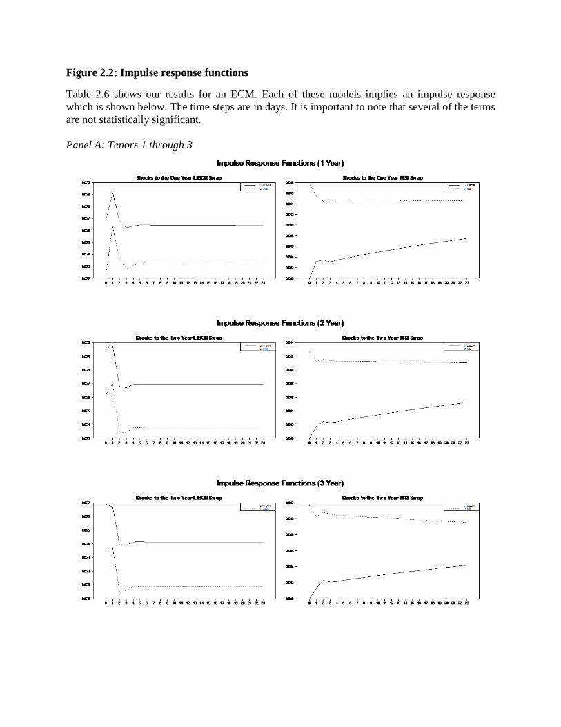
Figure 2.2: Impulse response functions
Table 2.6 shows our results for an ECM. Each of these models implies an impulse response
which is shown below. The time steps are in days. It is important to note that several of the terms
are not statistically significant.
Panel A: Tenors 1 through 3
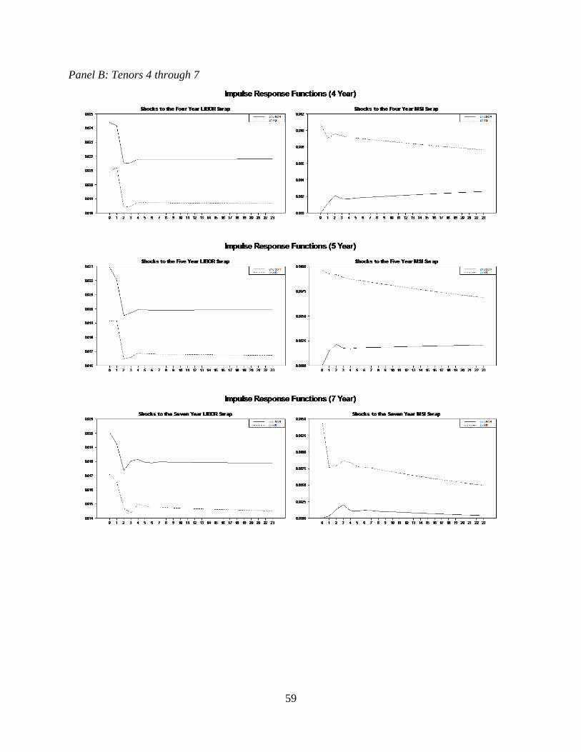
59
Panel B: Tenors 4 through 7
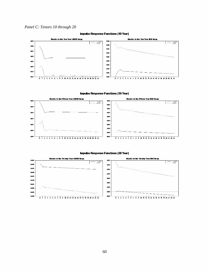
60
Panel C: Tenors 10 through 20
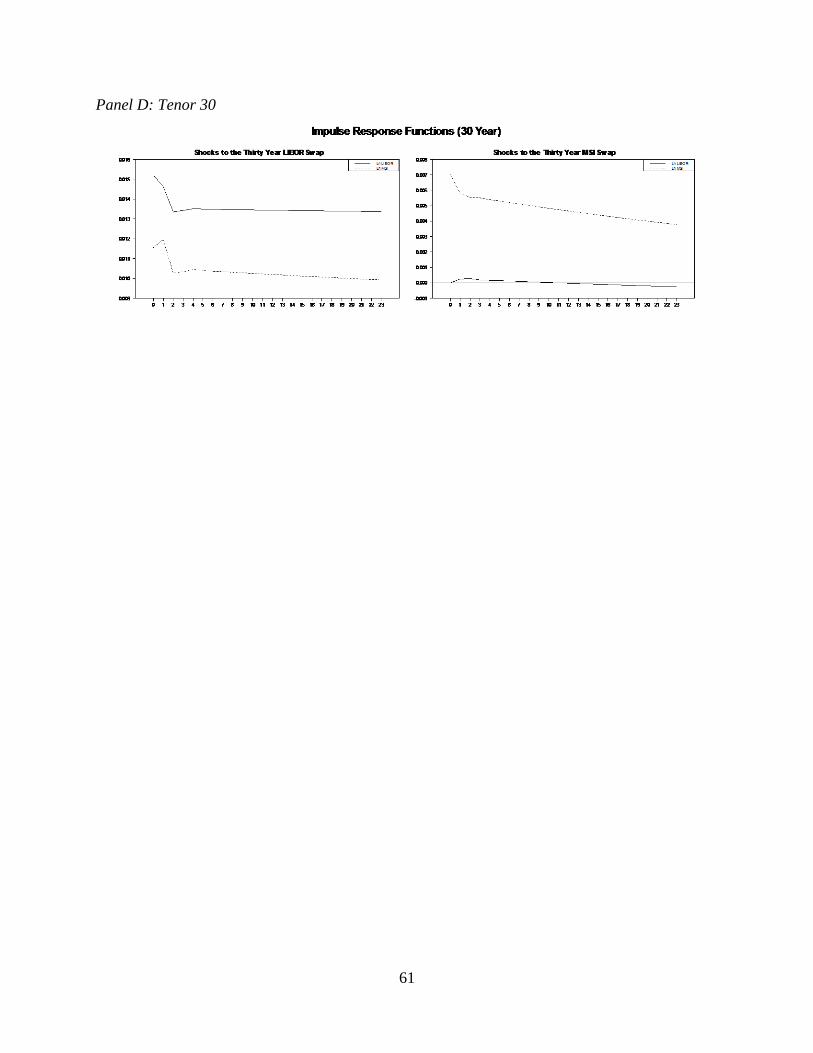
61
Panel D: Tenor 30
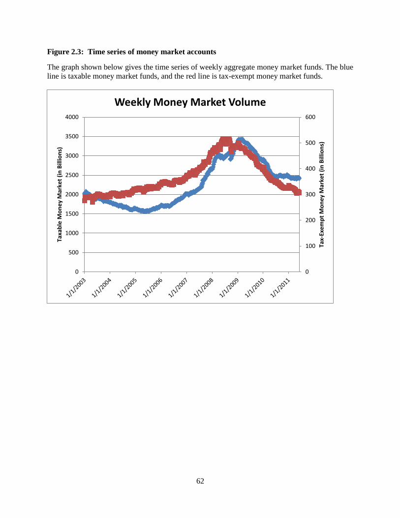
62
Figure 2.3: Time series of money market accounts
The graph shown below gives the time series of weekly aggregate money market funds. The blue
line is taxable money market funds, and the red line is tax-exempt money market funds.
0
100
200
300
400
500
600
0
500
1000
1500
2000
2500
3000
3500
4000
Tax-
Exe
mp
t M
on
ey
Mar
ket
(in
Bill
ion
s)
Taxa
ble
Mo
ne
y M
arke
t (i
n B
illio
ns)
Weekly Money Market Volume
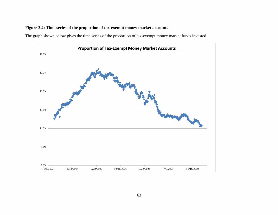
63
Figure 2.4: Time series of the proportion of tax-exempt money market accounts
The graph shown below gives the time series of the proportion of tax-exempt money market funds invested.
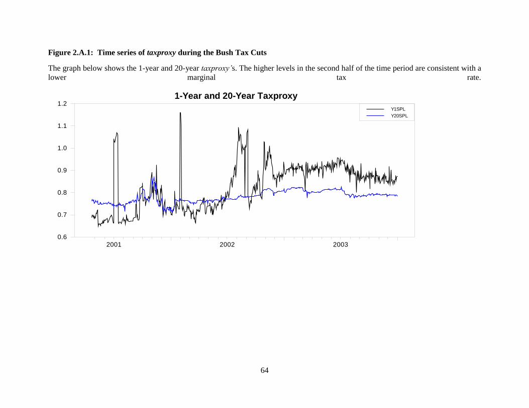
64
Figure 2.A.1: Time series of taxproxy during the Bush Tax Cuts
The graph below shows the 1-year and 20-year taxproxy’s. The higher levels in the second half of the time period are consistent with a
lower marginal tax rate.
1-Year and 20-Year Taxproxy
2001 2002 2003
0.6
0.7
0.8
0.9
1.0
1.1
1.2Y1SPL
Y20SPL
65
CHAPTER 3: ASYMMETRIC RELATIONSHIPS BETWEEN IMPLIED AND REALIZED
VOLATILITY
3.1. Introduction
There has always been a disconnect between expectations and reality. If unbiased, these
errors would be evenly distributed around implied expectations, but with a number of financial
time series this is not the case. This disconnect has implications about risk preferences.
Researchers have found a number of clever ways to get around this issue. For example, in much
of derivatives pricing, the endogenous relationship between risk and return is circumvented
through the use of risk-neutral space. Financial research has primarily focused on the first
statistical moment of datasets in the form of return, but there is evidence that the human
behaviors that price risk in returns also price risk in implied volatilities. Andersen and
Bondarenko (2007) find that implied volatility is almost always higher than realized volatility,
RV. In reference to this, Ang, et al. (2006) remarks that it is almost certainly the case that
implied and realized series behave differently--in this instance, because implied volatility will
have some risk premium embedded in it. The “Peso Problem” is another classic example of this
phenomenon. In order to gain deeper insight into the relationship between implied and realized
volatility, I use the CBOE Volatility Index, VIX, to proxy for implied volatility along with its
corresponding realized volatility.
There is a long and rich history of derivatives markets. Although forwards and futures
contracts have traded consistently for hundreds of years, options have had a more sporadic

66
history. Investors can easily trade on whether prices will go up or down, but sometimes investors
wish to trade on whether a series becomes more or less volatile. This trading could be
speculative or could represent a desire to hedge changes in volatility. A number of trading
strategies that provide liquidity are vulnerable to large price swings. In order to trade on
volatility, some type of asymmetric instrument must be trading. One of the earliest successful
options traders was Russell Sage who maintained a good-enough reputation to facilitate a well-
functioning options market. Since organized options exchanges did not exist, Sage could only
maintain his business by consistently honoring his financial contracts. He also developed one of
the most common volatility trading strategies the straddle8 (Jarrow and Chatterjea, 2013).
Although the options trading business was wildly profitable, only those with an enormous
amount of wealth and excellent reputations could facilitate this type of market. It wasn’t until
Black-Scholes-Merton that options trading once again became popular.
The advent of the Black-Scholes-Merton Option Pricing Model made option markets
viable. The Chicago Board Options Exchange opened on April 26, 1973, and trading on
volatility once again became a possibility for investors. A liquid options market allowed
investors to trade on a number of outcomes—including volatility. Cash settlement was also an
important innovation for these markets because it allowed investors to trade on an index without
needing the underlying. In 1983, cash settled options on stock indices began trading on the
CBOE. This allowed investors to easily trade on the volatility of large portions of the stock
market and paved the way for further innovation.
Brenner and Galai, in 1989, proposed the idea of an option that would allow investors to
hedge changes in volatility (formalized in a paper published in 1993). Whaley (1993), in that
8He even went by the nickname “Old Straddle”.
67
same issue of The Journal of Derivatives, laid out an argument for an index that would track
market volatility along with futures and options. He argued that this would allow option market
makers to hedge their volatility exposure much more cheaply than with options strategies. These
indices would allow futures contracts to be written on volatility, giving an almost costless means
for hedging volatility.
The original VIX, which is now called the VXO, was a weighted average of the one
month implied volatility taken from several at-the-money index options. These options were
written on the S&P 100 because, at the time, these index options were the most widely traded,
and, therefore, offered the most up-to-date price information. In order to better match recent
market conditions, the VIX was changed to be based on the S&P 500. Instead of a weighted
average, the VIX in its current form is designed to be a 30-day square root of an implied variance
swap to allow for a term structure of volatility9. The options used to compute this index have also
been changed to include a broader number of out-of-the-money options. These options are often
used by hedgers under widely used strategies like portfolio insurance.10 Not only has this index
provided a useful economic indicator and hedging instrument, the VIX and VXO have also
facilitated a number of studies on the dynamics of volatility.
The VIX index has provided an unprecedented way for investors to see the market’s
volatility expectations. As a measure of volatility, the VIX should have a number of unique
characteristics. The VIX and realized volatility are bounded from below by zero. Introspection
reveals that neither of these series should trend on towards infinity, but there is no upward bound
9 In the basic Black-Scholes-Merton Option Pricing Model the volatility increases by the square-
root of the time to maturity. The term structure of volatility allows for the influence of specific
events that are likely to affect volatility like Federal Reserve meetings. 10 Further details and arguments for this change can be found in Whaley (2009).
68
on their realizations. Although previous papers use a number of horse races to select among a
wide array of time series models (Chen, 2002; Christensen and Hansen, 2002; Ang et al., 2006;
Hung et al., 2009; and Kambourdis et al., 2013 among many others), I focus exclusively on a set
of threshold and smooth threshold autoregressive models to characterize these series.
My results reinforce several common findings in the literature. Although previous papers
have mixed results on the order of integration for the VIX, I find that the series is stationary
under a number of different specifications. The data does show a number of large positive spikes
that quickly revert back to normal levels indicating asymmetric behavior. My tests indicate that
the series has nonlinear and threshold effects. Though previous papers use basic threshold
effects, they do not test for a wide variety of threshold behaviors. This study is set apart because
I use a wide variety of STAR models to characterize the VIX in levels.
These findings present an important question for risk managers. Based on my results it is
not sufficient to use simply the most recent level of the VIX as a forward-looking indicator. My
results imply that there is a complex relationship between the VIX and realized volatility. Of the
information contained in the VIX, a large portion is derived from the previous 30 days’ realized
volatility. The presence of threshold effects also means that the normal approach is flawed. There
are times when almost all of the information necessary to forecast the VIX is contained in the
previous 30 days’ RV. Using the previous day’s VIX implies a unit root process. In stark contrast
to this common approach, I find that the VIX is stationary and follows an ESTAR process.
The remainder of this chapter is organized as follows: section 3.2 discusses the relevant
literature; in section 3.3, I discuss my data, hypothesis development, and methodology; section
3.4 reports the empirical findings; section 3.5 discusses several implications; and section 3.6
presents my conclusions.
69
3.2. Literature Review
There are two major lines of research that have characterized our understanding of
implied volatility series. The first is the research that looks at the time series behavior of implied
volatility and realized volatility. This research depends primarily on time series econometrics to
characterize these series. The second area of research develops option pricing models that use the
VIX or related index as the underlying. For these models some assumptions are made about the
stochastic process of the VIX. Empirical testing of these models and their correspondence, or
lack thereof, to observed prices reveals information about the underlying series.
Ang et al. (2006) mention that VIX should not be a perfect measure or forecast of
realized volatility because if it were, then it would need to have a zero risk premium. They also
use the VXO to examine the influence of aggregate risk on the cross-section of stock returns and
find that stocks with high sensitivity to the VXO have lower average returns. Several papers
point to the desire of investors to hedge volatility changes as they are related to investment
opportunities (Campbell, 1993; Campbell, 1996; Chen, 2002). These papers show that an
increase in volatility means that investment opportunities have declined. Under these models
risk-averse investors would prefer a hedging instrument that paid positive returns when volatility
increases.
Several assumptions lay the foundation for time series econometrics, the core of which is
that the data generating process is consistent over time (or for each sub period of time). Using
data that started before the US Civil War, Schwert and Pagan (1990) find that over several
distinct periods of time, the stock market is not covariance stationary. Correspondingly, Schwert
(1989) finds that de-monthly trended moving average models are not sufficient due to concerns
about covariance stationarity. I follow a number of papers that use nonlinear models to address
70
this issue. More recently, Schwert (2011) uses volatility data for a number of decades to put the
recent financial crisis in perspective. He argues that although there were long periods of
persistent high stock market volatility during the Great Depression, the pattern that appears since
then is strong mean reversion. This is consistent with my unit-root tests that find the VIX and its
corresponding realized volatility to be stationary.
The forecasting and, particularly, the prediction of increased stock market volatility have
attracted a lot of research. Christensen and Hansen (2002) use implied volatilities to construct a
forecasting series for realized return volatility. They use implied call, implied put, and historical
return volatility. They show that implied volatility is an efficient forecast of realized return
volatility. Hung, et al. (2009) use the asymmetric Glosten-Jagannathan-Runkle (1993) GARCH
model to compare one step ahead forecasts and find that combining the VIX with the GJR-
GARCH model was preferable for volatility forecasting. This is similar in form to the threshold
models I present.11 Similarly, Kambourdis, et al. (2013) use a number of GARCH and implied
volatility models to compare their ability to forecast stock market volatility. They find that
implied volatility models contain some additional information not found in GARCH models.
They also note that the presence of asymmetric effects significantly improves the performance of
their models.
Adhikari and Hilliard (2014) use the VIX and VXO to look at the Granger Causality
between each of these series and its corresponding realized volatility. They find that although
these series are designed to be forward looking, they depend substantially on the previous
11 The GJR-GARCH model can be represented as follows:
𝜎𝑡2 = 𝑘 + 𝛿𝜎𝑡−1
2 + 𝜎𝜖𝑡−12 + 𝜑𝜖𝑡−1
2 𝐼𝑡−1 + 𝑒𝑡
𝐼𝑡−1 {= 0 𝑖𝑓 𝜖𝑡−1 ≥ 0= 1 𝑖𝑓 𝜖𝑡−1 < 0

71
month’s realized volatility. Their data set ends right after the major volatility spike in October
2008. This spike seems to cause their unit root test to fail to reject the hypothesis of a unit root.
In addition to tests on the properties of the time series of the VIX, the VIX option pricing
literature gives insight into the stochastic properties of these second order moment series.
A recent literature has developed to price VIX derivatives. Since the VIX provides an
important market index for risk exposure, a number of derivatives that use it as the underlying
have started trading. Wang and Daigler (2009) do empirical testing of a number of option pricing
models by comparing their predicted option prices to the current option prices. They find that
simpler models work better, but no model is consistently accurate. A number of the stochastic
processes underlying these option pricing models are mean reverting, which is consistent with
my results.
Mencía and Sentana (2013) show the validity of a number of VIX option pricing models
by using VIX option and futures data. Because many of the models use a defined stochastic
process, they show a number of ways that the time series of VIX can be modeled. Many of their
models assume that the underlying series is stationary without a unit root; this is consistent with
my findings. My model of the VIX differs from theirs because instead of looking at the
nonlinearity present in the VIX data as long-run mean reversion to a changing long-run mean, I
use a threshold autoregressive setup. This allows me to model the VIX in several
characteristically different regions.
My research is set apart in several ways. Although a number of previous papers have
found evidence of nonlinear and threshold effects, I extend this approach to smooth transition
models. I also allow each of my series to have an independent smooth-transition autoregressive
(STAR) form, and I further show that this setup is statistically significant in pretesting.
72
Additionally, much of the previous literature has focused on our ability to predict future stock
market volatility. I look at predicting the VIX or future implied volatility. This is the cost of
purchasing options and is more applicable for risk managers as they consider the expected future
cost of short-term asymmetric hedging strategies.
3.3. Methodology
The historical VIX and VXO data is readily available online through the CBOE’s
website. I use daily closing prices to develop my testable dataset. The underlying for the VIX is
the S&P 500; the underlying for the older VXO is the S&P 100. Daily closing prices for these
two indices are readily available from a number of sources, and I pull them online from Yahoo!
Finance. Although the data is easy to get, there are some important sampling issues. In order to
model the influence of realized volatility on VIX, I use the realized volatility of the matching
forward-looking time period. The VIX is the square root of the fixed leg of a par variance swap
over the next 30 days as implied by a number of options assuming a term structure of volatility.
In order to appropriately match the realized volatility to the VIX, I take the VIX closing
price and label it VIX(t). Starting the next day, I calculate the realized return volatility using
closing prices going forward 30 calendar days. I label this RV(t). I then take the closing VIX on
the last trading day used in the realized volatility calculation and label this VIX(t+1). The next
trading day’s closing price is the first used in the calculation of RV(t+1). Since VIX is forward
looking, there is not an overlap in using the closing price and VIX measurement from the same
day. It is important to space out samples of the VIX to match my measure of realized volatility.

73
Even though the VIX has daily meaningful observations, the realized volatility measure does
not12.
The sample statistics are shown below. The mean and median of the volatility indices are
consistently higher than the realized volatility that they are designed to forecast, which is noted
by Andersen and Bondarenko (2007). The ranges of the volatility indices are smaller than their
corresponding realized volatility figures. This follows my observation that at the extremes, the
lagged VIX has little influence in forecasting itself. Correspondingly, the standard deviation for
the realized volatility measures is consistently higher for the volatility indices (this would be a
fourth order statistic in relation to stock returns). Each time series is positively skewed which
could be explained by each series being unbounded above. The series also show high levels of
excess kurtosis which is consistent with having a large number of small movements punctuated
by a few large movements.
The rejection of the Jarque-Bera statistic is similar to other financial datasets. A
decomposition of this measure (not shown) demonstrates that this rejection is not exclusively due
to just the skewness or kurtosis. Both statistics drive this measure to the rejection level. This also
gives further evidence for the Grünbichler and Longstaff (1996) derivatives pricing models
which use the CIR model for the stochastic process of VIX. The autocorrelations are low for
financial price data, and I test for the presence of a unit root as a robustness test. The cross
correlations indicate that these measures of volatility are not identical in their information
content.
12 Daily rolling windows would introduce tremendous false serial correlation because each day
one observation would change in my rolling sample at a time. This would be further exacerbated
by the presence of weekends.
74
The main hypothesis is that there are significant smooth threshold autoregressive effects
in the VIX and its related series. I begin by testing each series for stationarity using ADF tests
and Enders-Granger unit root tests to allow for asymmetric adjustment. I show that the model
specification for forecasting the VIX depends in large part on recent realized volatility and
lagged VIX. I test, initially, with a “sharp” threshold autoregressive test. Given the significance I
find, I use Teräsvirta’s (1994) test for delineating between an ESTAR and LSTAR models.
These pretests lay the foundation for the following model:
𝑉𝐼𝑋𝑡 = 𝛽0 + 𝛽1𝑉𝐼𝑋𝑡−1 + ⋯ + 𝛽𝑝𝑉𝐼𝑋𝑡−𝑝 + 𝛼1𝑅𝑉𝑡−1 + ⋯ + 𝛼𝑛𝑅𝑉𝑡−𝑝
+ 𝑔(𝑉𝐼𝑋𝑡−𝑑)[𝑏0 + 𝑏1𝑉𝐼𝑋𝑡−1 + ⋯ + 𝑏𝑝𝑉𝐼𝑋𝑡−𝑝 + 𝑎1𝑅𝑉𝑡−1 + ⋯ + 𝑎𝑝𝑅𝑉𝑡−𝑝] + 휀𝑡
where,
0 ≤ 𝑔(𝑉𝐼𝑋𝑡−𝑑) ≤ 1
The coefficients, αi, βi, ai, and bi are the coefficients estimated for the VIX. In the above equation
AR(p) models are present for the lagged VIX and lagged realized volatility, RV. The coefficients
are jointly estimated in each regime. Here g(VIXt-d) is the transition function, and d is the delay
parameter. I define the transition function in one of the following ways:
For an LSTAR model,
𝑔𝐿𝑆𝑇𝐴𝑅(𝑉𝐼𝑋𝑡−𝑑) = [1 + exp(−𝛾(𝑉𝐼𝑋𝑡−𝑑 − 𝑐))]−1
For an ESTAR model,
𝑔𝐸𝑆𝑇𝐴𝑅(𝑉𝐼𝑋𝑡−𝑑) = 1 − exp[−𝛾(𝑉𝐼𝑋𝑡−𝑑 − 𝑐)2]
Here γ is a measure of how fast the transition function moves between 0 and 1. The estimated
coefficient c is the center of the transition region. Introspection shows that even if the most
recent 30 day realized volatility is 0, the forward-looking market-driven VIX would certainly not
be 0. I also propose that the information contained in the VIX and recent RV depends on the
75
previous observations of the VIX and RV in the sense that the AR equation’s coefficients depend
on the previous observations of the VIX and RV. Congruous with this observation, I find that the
level of mean reversion for the VIX is regime dependent.
3.4. Empirical Findings
A number of previous papers have wrestled with the question of whether or not the time
series of VIX and realized volatility are stationary (Wang and Daigler, 2009). I use stationary as
oppose to trend stationary because there should not be any persistent long-term trends in either of
these terms13. Ang et al. (2006) argue that although the similar VXO series has high
autocorrelation, it is likely to be stationary. Adhikari and Hilliard (2014) find that the VIX time
series is not stationary in levels, but their dataset’s last several observations include the
beginning of the recent financial crisis. It is certainly not the case that the time series behavior of
the VIX is non-stationary in levels. This would mean that since the series is bounded from
below, we should expect it to trend on towards positive infinity. In the same way, I expect
realized volatility to be stationary. In order to have cohesive test conclusions later on (that are
based on levels), it is important to show that the underlying series are stationary, but there is
another contravening factor that clouds this type of testing.
The core hypothesis of this paper is the presence of nonlinear effects in levels.
Nonlinearity reduces the power of unit-root tests in the same way as structural breaks14. In order
13 Although the VIX is related to other economic variables that display a trend, a long term trend
would push the series either to 0 or ∞. Neither of these is viable given the underlying meaning of
the VIX. 14 Structural breaks are actually a special case of the threshold autoregressive model where time
is the threshold variable. The TAR model is itself a special case of smooth-transition threshold
autoregressive models.

76
to test for the presence of a unit-root, I begin with Augmented Dickey-Fuller, ADF, testing.
Since there are several large spikes in the later part of the time series, I allow for the presence of
deterministic trend terms and follow Dolado et al. (1990) to eliminate each drift term. The results
in Table 3.2 show that there is a significant constant drift term in each series, but in each case I
reject the null hypothesis of a unit-root. The large spikes in the second half of the dataset are
likely the cause of the significant trend term. I follow a general-to-specific methodology by
starting with 12 lags in each case, which is approximately one year of previous observations.
Since I show later that there are significant nonlinearity effects in the model, this is a stronger
result than necessary. In order to further see if nonlinearity is present in the series, I test for a unit
root in the presence of asymmetric adjustment.
Enders and Granger (1998) present an approach to unit root testing in the presence of
asymmetric adjustment. They show this in the context of threshold and momentum threshold
models, and I test under each structure. The threshold model uses a lagged observation of the
variable of interest; the momentum threshold model uses a lagged first difference. As the
attractor, they use zero, a constant, or a linear trend term. Since the realized volatility (and
correspondingly, VIX) is bounded from below at zero, I test only with the constant and linear
trend setups. The results for these tests are shown in Table 3.3. With the TAR model and a
constant attractor, the S&P 500 realized volatility is significant at the 5% level. In all other cases
I reject the presence of a unit root at a greater than 1% level. Kιlιҫ (2011) puts forward a unit-
root test in the presence of an ESTAR model. For an ESTAR model, a unit root in the internal
portion of the model is acceptable as long as it is mean-reverting in the outer region. In order to
test the outer region, Kιlιҫ puts forward the following model:
∆𝑦𝑡 = ∑ 𝛿𝑖∆𝑦𝑡−𝑖
𝑝
𝑡=1
+ 𝜙𝑦𝑡−1(1 − exp(−𝛾𝑧𝑡2)) + 𝑢𝑡
77
Here, y represents the demeaned, detrended VIX. Starting at p = 12, I select p based on the BIC.
The variable ϕ is the unit-root test coefficient. γ is the rate of conversion from one regime to
another. zt is set to Δyt-d. The delay parameter, d, is found using the smallest RSS. The results are
shown in Table 3.4. Similar to each of the other unit-root tests done so far, I strongly reject the
presence of a unit root. This is consistent with previous models that have assumed a stationary
model of the VIX and volatility (see Whaley’s, 1993, critique of his own model).
The Enders-Granger test also gives other useful statistics for characterizing the behavior
of the data. Once the presence of a unit root has been rejected, the equality statistic can be used
to test whether the adjustment is symmetrical. Here I find mixed results. Based on the RSS the
TAR model is a better fit for the VIX series; because under the TAR model, the VIX adjustment
terms are significantly different. This means that there may be a region where the VIX is much
closer to a unit-root relative to the other region. For the RV series, the momentum threshold
model gives a lower RSS. Here again the adjustment terms are significantly different from each
other indicating regional differences. Since I have found that there is evidence of threshold
effects, I move next to a set of pretests for threshold models.
I begin the identification of the nonlinearity by pretesting for threshold behavior using a
test that assumes an abrupt break between regimes based on a lagged term. I select an AR(p)
model by using the AIC and BIC. The best fit for the VIX is an AR(2) model, and the best fit for
the realized volatility series is an AR(1). Since I am moving towards a VAR model, I use an
AR(2) model in both cases for the threshold testing. In each case, p-values are generated from
1000 random draws. I also test each variable using the other variable as the threshold variable,
and I run the tests under the momentum threshold setup as well. The threshold testing in Table
78
3.5 shows a number of significant results. Since threshold effects are present, I move, next, to a
pretest that includes a broader range of threshold behaviors.
Teräsvirta (1994) develops a model that allows for testing between an LSTAR and an
ESTAR model. This test involves using the higher-order Taylor-Series coefficients and testing
several conditional hypotheses about these statistics. The preliminary test uses a null hypothesis
of linearity. As shown in Table 3.6, I reject linearity in several instances. Since financial markets
quickly incorporate information, I expect the delay parameter to be small for my STAR model.
For d equal to 1 or 2, I strongly reject the null hypothesis of a linear model. Once linearity is
rejected, the general rule for picking between an LSTAR and ESTAR model is to see whether
the rejection of H02 is stronger than the rejection of H01 or H03. When true, the ESTAR is
likely to be the best fit. An ESTAR model will also likely reject H12. This is precisely the
pattern given by the results for d=2. Unfortunately, the reliability of these tests is reduced by the
presence of data asymmetry. There are also several configurations where the LSTAR model is
approximated by part of an ESTAR model. To compare these models, I begin the estimation
process.
The data in Figure 3.2 shows signs of an ESTAR model visually and through testing.
Visually, there seems to be a greater disconnect between the VIX and RV when realized
volatility is very low or very high. I develop an ESTAR model and begin with lag length tests.
With an ESTAR model, there are two regions. One region is found where the transition function,
g, is zero (coefficients labeled 1). The other region is where the lagged VIX is far from the
threshold (the sum of coefficients 1 and 2). Between these regions the model smoothly
transitions from one to the other. Using log-likelihood tests I fail to reject the null hypothesis that
the third lag variables are zero. In order to select the correct delay parameter for the regime
79
switching, I use the lag length found earlier and vary the delay parameter. A delay parameter of 2
gave the lowest RSS. Once the delay parameter was selected, I recalculated the lag length tests to
get the lag length of 2. Iterating between each of these selection criteria gave a consistent model
of 2 lags with a delay parameter of 2, which is shown below. The regression results in Table 3.7
show starkly different characteristics for each region. Because I use a nonlinear model, the
statistical significance shown cannot be directly used for hypothesis testing, but the relative
magnitudes of the t-statistics do communicate something about the nature of the underlying
variables. Normally, one would expect the most recent observation to contain the most
information, but the VIX contains a number of significant, short-lived spikes. When VIXt is a
spike, both of the last two VIX observations fit poorly. When VIXt-1 is a spike, it is not as
informative as VIXt-2. Using a delay parameter of 2, meaning VIXt-2 is used in the transition
function, fits better because it solves this spiking issue. I, next, remove different parts from the
above model to see whether both series are statistically significant.
The most recent VIX and most recent RV both contain a lot of overlapping information
which can be seen in simple linear models. Within the ESTAR model that I develop, I remove all
the lags of each series to see if they are altogether statistically significant. I use likelihood ratio
tests which can be seen in Panel B of Table 3.7. I first exclude all the lags of RV. If it is not
valuable in forecasting the VIX, then I should fail to reject the null hypothesis that these
coefficients are zero. This is also a test of Granger Causality because a failure to reject would
mean that the lags of RV are not significantly useful in forecasting the VIX. I strongly reject the
null hypothesis meaning that the RV Granger Causes (or is useful in forecasting) the VIX.
Second, I exclude all of the lags of the VIX from the model. If a dominant amount of the useful
forecasting information is included in the RV and the VIX is not incrementally useful, then I

80
would expect to fail to reject for the VIX exclusion. I find the opposite and strongly reject that
the VIX terms are jointly not useful in forecasting. Typically, a general-to-specific method is
common practice for time series models, but in Table 3.7 there are a number of lags that seem to
be insignificant (once again the t-stats are not informative in nonlinear models). In order to
examine the significance of these lags further, I use log-likelihood tests to check each of the
second lags individually. I start with a single lag of each variable in each region. I then add a
single additional lag in each region and test this additional variable for significance. The results
are shown in Panel A of Table 3.8.
On the one hand, the results of the log-likelihood tests fail to reject that the additional lag
of realized volatility lag is zero. On the other hand, the tests strongly reject that the coefficients
on the additional lags of the VIX are zero. To further avoid over-fitting my model, I also
calculate the AIC and BIC for a number of different lag configurations which are shown in Panel
B of the aforementioned table. Although the log-likelihood tests indicate using two lags in each
region for the VIX and a single lag in each region for the RV, the AIC and BIC both select a
single lag for each variable in each region except for in region 2 for the VIX. Having selected a
more parsimonious model, I next move to estimation.
The previous tests have led to an ESTAR model that uses a single lag of the realized
volatility and 1 or 2 lags of the VIX depending on the region. In the region very close to the
threshold variable, I use a single lag of the VIX. I region 2, when the threshold variable is far
from the threshold variable, I use two lags of the VIX. The estimated model is shown in Table
3.9. Interestingly, the previous period’s RV is incorporated on a nearly one-to-one basis near to
the threshold value. Hence, in normal markets near the historical average, the VIX incorporates
almost all of the previous period’s realized volatility. As the threshold variable moves further
81
from this normal rage, a much smaller amount of the previous period’s realized volatility is
incorporated into the VIX. When volatilities are very high or very low, the VIX depends less on
RV. This is further explored in the model’s long-run means.
Since the models coefficients depend on the threshold variable, I use the average of
realized volatility and the model’s regional coefficients to develop a table of coefficients and
long-run means. The model’s long-run means are dependent on the threshold variable. This
pattern is shown in Figure 3.3. The results are also shown in Table 3.9.
The presence of ESTAR regions shows starkly different behaviors in each region. Near
the threshold value, the previous RV is almost entirely incorporated, but the previous lags of the
VIX have a very small influence on the one-step ahead forecasts. In the fringe region (at very
low or very high levels) a little over one third of the previous realized volatility is incorporated in
the VIX. This is a much smaller amount than in the middle region. In this fringe region, the VIX
also displays more persistence. This is consistent with the greater disconnect observed in the
fringe regions. Even if RV were to be nearly zero for several days, the VIX would remain higher.
This similar disconnect is observed when RV is spiking. Although the VIX is almost always
higher than RV, traders know that a large spike will quickly revert to normal levels.
There is an argument that suggests interest rates must be stationary because over the past
century they have been fairly similar to what they were in some of the most ancient cultures
(Cochrane, 1991). With time series modeling, each model implies a long-run mean (or lack of
one). Thus, similarly, I use the average of realized volatility and the ESTAR model to look at
how the long-run mean varies with the threshold value. The results below show that the series is
generally reverting towards a value of 13.5, but when the previous VIX observation is close to
18, this long-run reversion point increases. This also shows that the behavior of the VIX in each
82
extreme is fairly similar. Near the median, the forecasted VIX depends primarily on previous
RV, but in the extremes, the most recent value of the VIX has a greater impact on the one-step
ahead forecast. In these extremes, the previous RV has a smaller influence on the VIX. These
dynamics are consistent with previous literature that has said that indices like the VIX hold some
information that recent realized volatility does not.
The VIX and RV time series are based on the second order moments of returns. In order
to further characterize these series, I also pretested for the GARCH behaviors in these series.
Since this would be the standard deviation of a standard deviation, this is a fourth order
characteristic. In results not shown, I find GARCH effects similar to almost any other financial
variable. These fourth-order effects generally lower the power of tests in levels, but since my
tests still found significant effects I did not build the GARCH effects into my model.
3.5. Implications
There has been an extraordinary amount of capital invested into volatility tracking
indices. The presence of volatility speculation gives a unique window into how individuals view
volatility. Previous literature has found that the information contained in a volatility index is
likely not the same as the information contained in the most recent month’s realized volatility. I
show that in addition to the above effects, there are also marked differences that depend on the
region in which the recent VIX levels have occurred. This is important for anyone in the options
market and particularly important for those who are using or forecasting implied volatilities for
value-at-risk studies.
Financial firms direct a significant amount of resources to various risk management
measures. The implications of my findings are that using the VIX or realized volatility alone is
83
not sufficient for forecasting future volatility levels. Even using both these series is not sufficient
because they contain threshold effects; hence, in some regions only one of the above volatility
indicators is useful. Although the VIX is designed to be forward looking, a large portion of its
information is contained in the previous period’s realized volatility. Risk managers must use all
of the information contained in these series in order to accurately forecast volatility.
3.6. Conclusions
I have shown that the VIX is not only distributed asymmetrically, it also has nonlinear
threshold effects. In contrast to many previous studies, I have shown that the VIX is stationary
which is consistent with our theoretical understanding of the statistical moments of financial
data. The level of mean-reversion and, correspondingly, the ability to reject a unit-root process is
asymmetric in Enders-Granger tests. This indicates the presence of a nonlinear data generating
process. I pretest for both threshold and smooth threshold autoregressive effects and find
significant evidence for both. Using Teräsvirta’s (1994) pretest for picking a LSTAR or ESTAR
model, testing suggests an ESTAR model is a better fit. Harmoniously, I estimate an ESTAR
model that confirms my suspicions that there are economically and statistically significant
smooth threshold effects in the time series of the VIX. These findings are important for a number
of reasons. It can be argued that the VIX captures more about market psychology than recent
realized volatility. My model indicates that when recent VIX levels are far from their threshold
value the most recent VIX and RV observations have some level of influence on the predicted
next observation. Close to the threshold value, the VIX is not very influential for forecasting and
most of the next VIX comes from the recent RV. Throughout both regions the RV plays an
important part in predicting the VIX, but this influence is much smaller at the extremes. Standard

84
industry practice is to use some weighted average of implied volatilities for model calibration.
However, this approach ignores non-linear and regime switching possibilities which are clearly
present in these time series. Risk managers must take into account these effects when building
their term structure of volatility for pricing and forecasting.
85
REFERENCES
Adhikari, B. & Hilliard, J. (2014). The VIX, VXO and realized volatility: a test of lagged and
contemporaneous relationships. International Journal of Financial Markets and Derivatives 3,
222-240.
Andersen, T. & Bondarenko, O. (2007). Construction and interpretation of a model-free implied
volatility. Unpublished working paper. National Bureau of Economic Research.
Ang, A., Hodrick, R., Xing, Y., & Zhang, X. (2006). The cross-section of volatility and expected
returns. The Journal of Finance 61, 259-299.
Black, F. & Scholes, M. (1973). The pricing of options and corporate liabilities. Journal of
Political Economy 81, 637-659.
Brenner, M. & Galai, D. (1989). New financial instruments for hedging changes in volatility.
Financial Analysts Journal 45, 61-65.
Brenner, M. & Galai, D. (1993). Hedging volatility in foreign currencies. The Journal of
Derivatives 1, 53-58.
Campbell, J. (1993). Intertemporal asset pricing without consumption data. American Economic
Review 83, 298-345.
Campbell, J. (1996). Understanding risk and return. Journal of Political Economy 104, 298-345.
Chen, J. (2002). Intertemporal, CAPM and the cross-section of stock returns. Unpublished
working paper. University of Southern California.
Christensen, B. & Hansen, C. (2002). New evidence on the implied-realized volatility relation.
The European Journal of Finance 8, 187-205.
Cochrane, J. (1991). Pitfalls and opportunities: what macroeconomists should know about unit
roots. NBER Macroeconomics Annual 6, 201-210.
Detemple, J. & Osakwe, C. (2000). The valuation of volatility options. European Finance
Review 4, 21-50.
Dolado, J., Jenkinson, T., & Sosvilla-Rivero, S. (1990). Cointegration and unit roots. Journal of
Economic Surveys 4, 249-273.

86
Enders, W. & Granger, C. (1998). Unit-root tests and asymmetric adjustment with an example
using the term structure of interest rates. Journal of Business & Economic Statistics 16, 304-311.
Glosten, L., Jaganathan, R., & Runkle, D. (1993). On the relation between the expected value
and the volatility of nominal, excess return on stocks. The Journal of Finance 48, 1779-1801.
Grünbichler, A. & Longstaff, F. (1996). Valuing futures and options on volatility. Journal of
Banking & Finance 20, 985-1001.
Hung, J., Ni, R., & Chang, M. (2009). The information contents of VIX index and ranged-based
volatility on volatility forecasting performance of S&P 500. Economics Bulletin 29, 2596-2604.
Jarrow, R. & Chatterjea, A. (2013). An Introduction to Derivative Securities, Financial Markets,
and Risk Management. W. W. Norton and Company-New York, London.
Kambouroudis, D., McMillan, D., & Tsakou, K. (2013). Forecasting stock return volatility: a
comparison of GARCH models and implied volatility. Unpublished working paper. University of
Stirling.
Kιlιҫ, R.(2011). Testing for a unit root in a stationary ESTAR process. Econometric Reviews 30,
274-302.
Luukkonen, R., Saikkonen, P., & Teräsvirta, T. (1988). Testing linearity against smooth
transition autoregressive models. Biometrika 57, 491-499.
Mencía, J. & Sentana, E. (2013). Valuation of VIX derivatives. Journal of Financial Economics
108, 367-391.
Merton, R. (1973). Theory of rational call option pricing. Bell Journal of Economics and
Management Science 4, 141-183.
Pagan, A. & Schwert, G. (1990). Alternative models for conditional stock market volatility.
Journal of Econometrics 45, 267-290.
Schwert, G. (1989). Why does stock market volatility change over time? The Journal of Finance
44, 1115-1153.
Schwert, G. (2011). Stock volatility during the recent financial crisis. European Financial
Management 17, 789-805.
Skalin, J. & Teräsvirta, T. (1999). Another look at Swedish business cycles, 1861-1988. Journal
of Applied Econometrics 14, 359-378.
Teräsvirta, T. (1994). Specification, estimation, and evaluation of smooth transition
autoregressive models. Journal of the American Statistical Association 89, 208-218.

87
Wang, Z. & Daigler, R. (2009). The performance of VIX option pricing models: empirical
evidence beyond simulation. Unpublished working paper. Florida International University.
Whaley, R. (1993). Derivatives on market volatility. The Journal of Derivatives 1, 71-84.
Whaley, R. (2009). Understanding the VIX. Journal of Portfolio Management 35, 98-105.
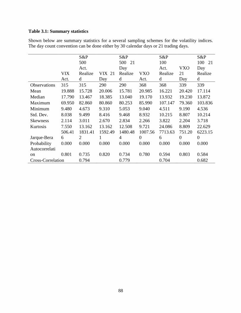
88
Table 3.1: Summary statistics
Shown below are summary statistics for a several sampling schemes for the volatility indices.
The day count convention can be done either by 30 calendar days or 21 trading days.
VIX
Act.
S&P
500
Act.
Realize
d
VIX 21
Day
S&P
500 21
Day
Realize
d
VXO
Act.
S&P
100
Act.
Realize
d
VXO
21
Day
S&P
100 21
Day
Realize
d
Observations 315 315 290 290 368 368 339 339
Mean 19.888 15.728 20.006 15.781 20.985 16.221 20.420 17.114
Median 17.790 13.467 18.385 13.040 19.170 13.932 19.230 13.872
Maximum 69.950 82.860 80.860 80.253 85.990 107.147 79.360 103.836
Minimum 9.480 4.673 9.310 5.053 9.040 4.511 9.190 4.536
Std. Dev. 8.038 9.499 8.416 9.468 8.932 10.215 8.807 10.214
Skewness 2.114 3.011 2.670 2.834 2.266 3.822 2.204 3.718
Kurtosis 7.550 13.162 13.162 12.508 9.721 24.086 8.809 22.629
Jarque-Bera
506.41
6
1831.41
2
1592.49
1
1480.48
4
1007.56
0
7713.63
6
751.20
0
6223.15
0
Probability 0.000 0.000 0.000 0.000 0.000 0.000 0.000 0.000
Autocorrelati
on 0.801 0.735 0.820 0.734 0.780 0.594 0.803 0.584
Cross-Correlation 0.794
0.779
0.704
0.682
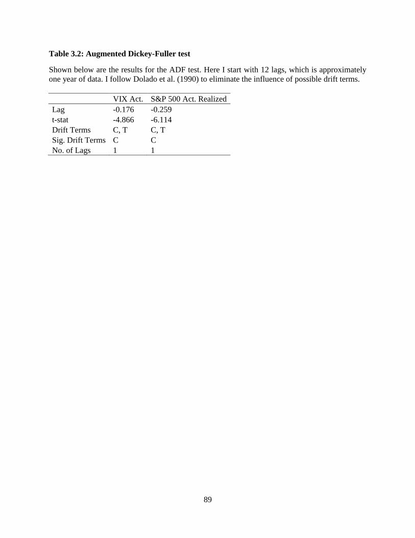
89
Table 3.2: Augmented Dickey-Fuller test
Shown below are the results for the ADF test. Here I start with 12 lags, which is approximately
one year of data. I follow Dolado et al. (1990) to eliminate the influence of possible drift terms.
VIX Act. S&P 500 Act. Realized
Lag -0.176 -0.259
t-stat -4.866 -6.114
Drift Terms C, T C, T
Sig. Drift Terms C C
No. of Lags 1 1
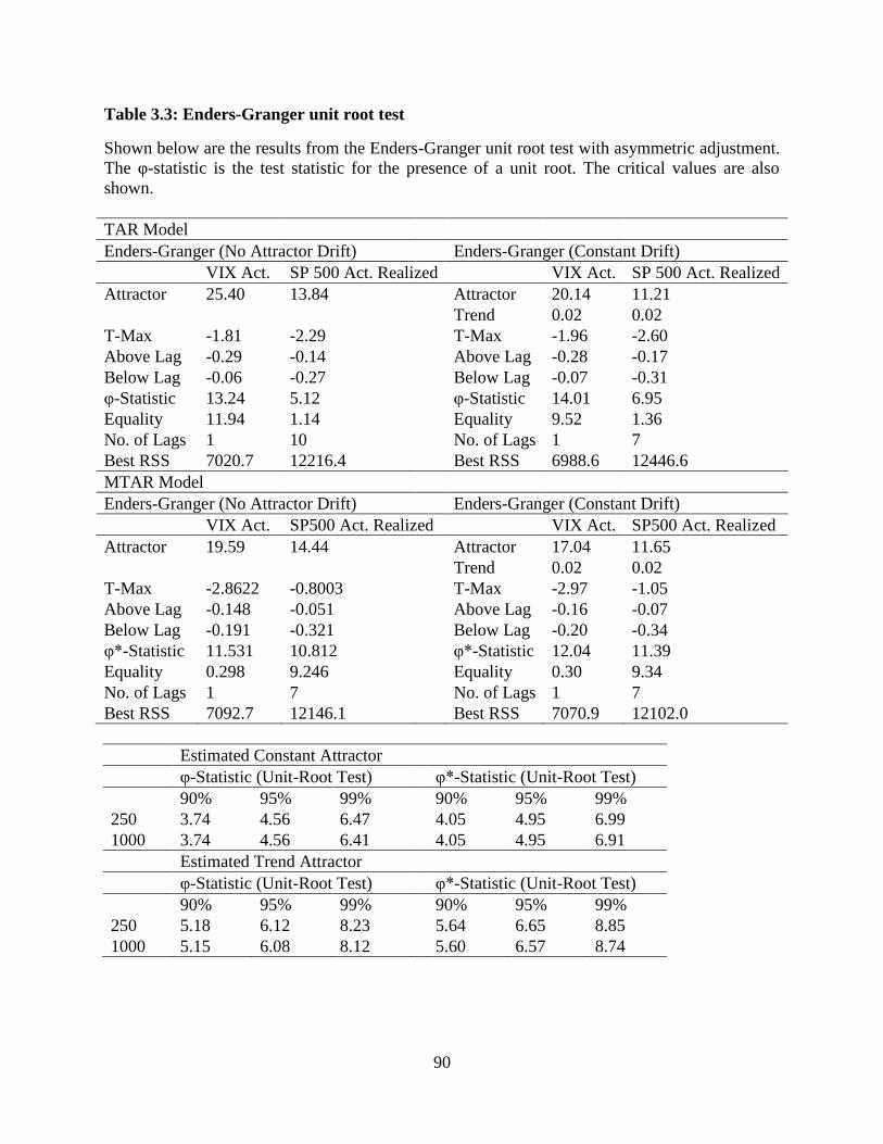
90
Table 3.3: Enders-Granger unit root test
Shown below are the results from the Enders-Granger unit root test with asymmetric adjustment.
The φ-statistic is the test statistic for the presence of a unit root. The critical values are also
shown.
TAR Model
Enders-Granger (No Attractor Drift)
Enders-Granger (Constant Drift)
VIX Act. SP 500 Act. Realized
VIX Act. SP 500 Act. Realized
Attractor 25.40 13.84
Attractor 20.14 11.21
Trend 0.02 0.02
T-Max -1.81 -2.29
T-Max -1.96 -2.60
Above Lag -0.29 -0.14
Above Lag -0.28 -0.17
Below Lag -0.06 -0.27
Below Lag -0.07 -0.31
φ-Statistic 13.24 5.12
φ-Statistic 14.01 6.95
Equality 11.94 1.14
Equality 9.52 1.36
No. of Lags 1 10
No. of Lags 1 7
Best RSS 7020.7 12216.4
Best RSS 6988.6 12446.6
MTAR Model
Enders-Granger (No Attractor Drift)
Enders-Granger (Constant Drift)
VIX Act. SP500 Act. Realized
VIX Act. SP500 Act. Realized
Attractor 19.59 14.44
Attractor 17.04 11.65
Trend 0.02 0.02
T-Max -2.8622 -0.8003
T-Max -2.97 -1.05
Above Lag -0.148 -0.051
Above Lag -0.16 -0.07
Below Lag -0.191 -0.321
Below Lag -0.20 -0.34
φ*-Statistic 11.531 10.812
φ*-Statistic 12.04 11.39
Equality 0.298 9.246
Equality 0.30 9.34
No. of Lags 1 7
No. of Lags 1 7
Best RSS 7092.7 12146.1
Best RSS 7070.9 12102.0
Estimated Constant Attractor
φ-Statistic (Unit-Root Test)
φ*-Statistic (Unit-Root Test)
90% 95% 99%
90% 95% 99%
250 3.74 4.56 6.47
4.05 4.95 6.99
1000 3.74 4.56 6.41
4.05 4.95 6.91
Estimated Trend Attractor
φ-Statistic (Unit-Root Test)
φ*-Statistic (Unit-Root Test)
90% 95% 99%
90% 95% 99%
250 5.18 6.12 8.23
5.64 6.65 8.85
1000 5.15 6.08 8.12
5.60 6.57 8.74
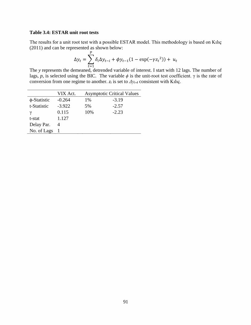
91
Table 3.4: ESTAR unit root tests
The results for a unit root test with a possible ESTAR model. This methodology is based on Kιlιҫ
(2011) and can be represented as shown below:
∆𝑦𝑡 = ∑ 𝛿𝑖∆𝑦𝑡−𝑖
𝑝
𝑡=1
+ 𝜙𝑦𝑡−1(1 − exp(−𝛾𝑧𝑡2)) + 𝑢𝑡
The y represents the demeaned, detrended variable of interest. I start with 12 lags. The number of
lags, p, is selected using the BIC. The variable ϕ is the unit-root test coefficient. γ is the rate of
conversion from one regime to another. zt is set to Δyt-4 consistent with Kιlιҫ.
VIX Act.
Asymptotic Critical Values
ϕ-Statistic -0.264
1% -3.19
t-Statistic -3.922
5% -2.57
γ 0.115
10% -2.23
t-stat 1.127
Delay Par. 4
No. of Lags 1
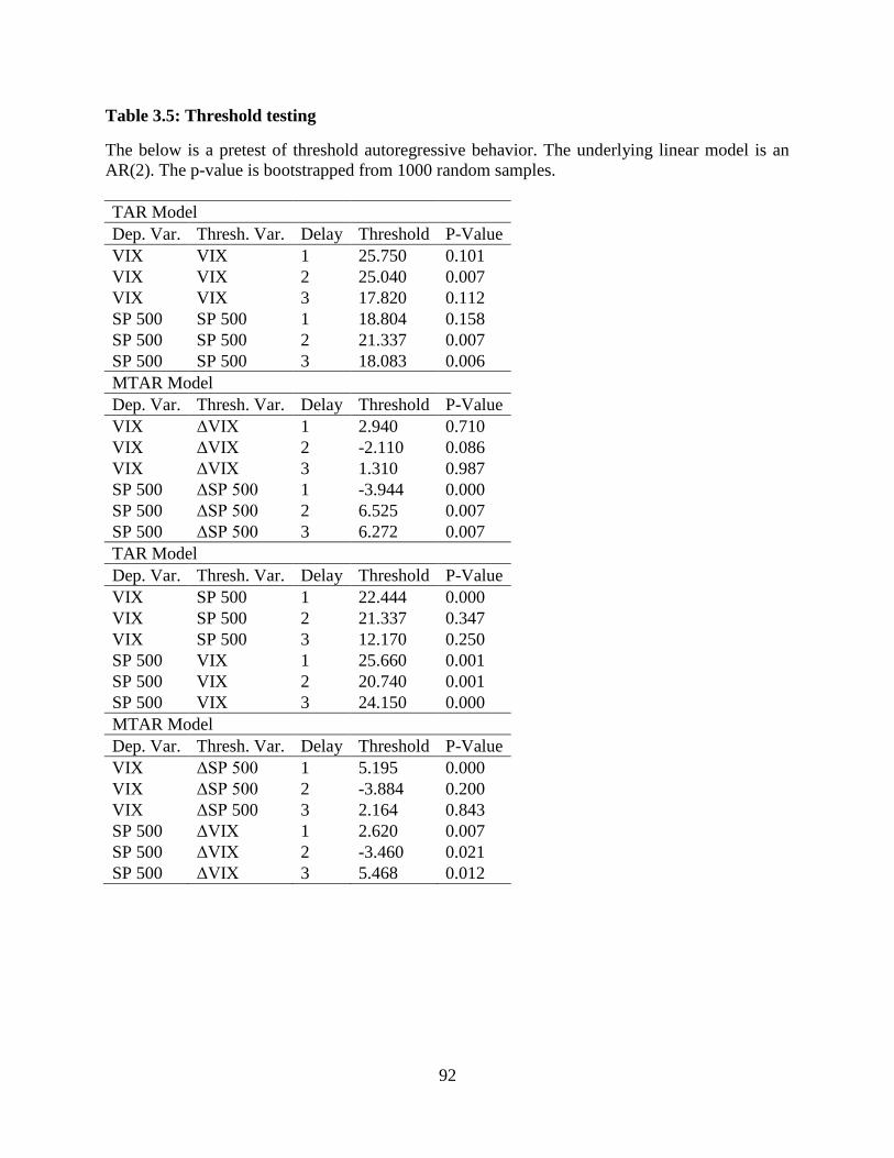
92
Table 3.5: Threshold testing
The below is a pretest of threshold autoregressive behavior. The underlying linear model is an
AR(2). The p-value is bootstrapped from 1000 random samples.
TAR Model
Dep. Var. Thresh. Var. Delay Threshold P-Value
VIX VIX 1 25.750 0.101
VIX VIX 2 25.040 0.007
VIX VIX 3 17.820 0.112
SP 500 SP 500 1 18.804 0.158
SP 500 SP 500 2 21.337 0.007
SP 500 SP 500 3 18.083 0.006
MTAR Model
Dep. Var. Thresh. Var. Delay Threshold P-Value
VIX ΔVIX 1 2.940 0.710
VIX ΔVIX 2 -2.110 0.086
VIX ΔVIX 3 1.310 0.987
SP 500 ΔSP 500 1 -3.944 0.000
SP 500 ΔSP 500 2 6.525 0.007
SP 500 ΔSP 500 3 6.272 0.007
TAR Model
Dep. Var. Thresh. Var. Delay Threshold P-Value
VIX SP 500 1 22.444 0.000
VIX SP 500 2 21.337 0.347
VIX SP 500 3 12.170 0.250
SP 500 VIX 1 25.660 0.001
SP 500 VIX 2 20.740 0.001
SP 500 VIX 3 24.150 0.000
MTAR Model
Dep. Var. Thresh. Var. Delay Threshold P-Value
VIX ΔSP 500 1 5.195 0.000
VIX ΔSP 500 2 -3.884 0.200
VIX ΔSP 500 3 2.164 0.843
SP 500 ΔVIX 1 2.620 0.007
SP 500 ΔVIX 2 -3.460 0.021
SP 500 ΔVIX 3 5.468 0.012
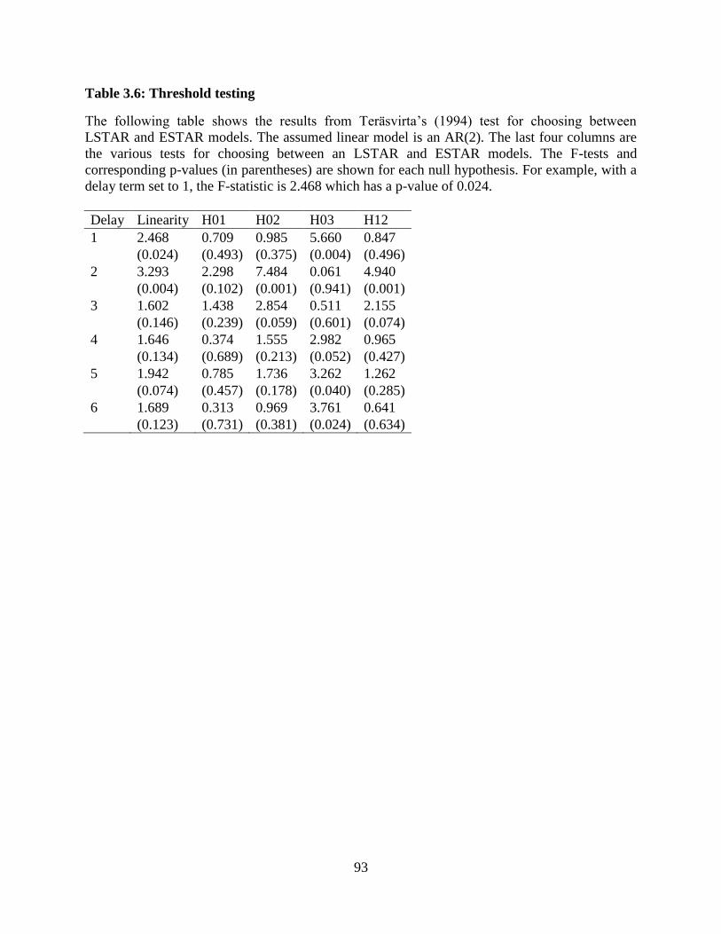
93
Table 3.6: Threshold testing
The following table shows the results from Teräsvirta’s (1994) test for choosing between
LSTAR and ESTAR models. The assumed linear model is an AR(2). The last four columns are
the various tests for choosing between an LSTAR and ESTAR models. The F-tests and
corresponding p-values (in parentheses) are shown for each null hypothesis. For example, with a
delay term set to 1, the F-statistic is 2.468 which has a p-value of 0.024.
Delay Linearity H01 H02 H03 H12
1 2.468 0.709 0.985 5.660 0.847
(0.024) (0.493) (0.375) (0.004) (0.496)
2 3.293 2.298 7.484 0.061 4.940
(0.004) (0.102) (0.001) (0.941) (0.001)
3 1.602 1.438 2.854 0.511 2.155
(0.146) (0.239) (0.059) (0.601) (0.074)
4 1.646 0.374 1.555 2.982 0.965
(0.134) (0.689) (0.213) (0.052) (0.427)
5 1.942 0.785 1.736 3.262 1.262
(0.074) (0.457) (0.178) (0.040) (0.285)
6 1.689 0.313 0.969 3.761 0.641
(0.123) (0.731) (0.381) (0.024) (0.634)
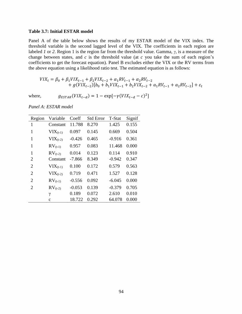
94
Table 3.7: Initial ESTAR model
Panel A of the table below shows the results of my ESTAR model of the VIX index. The
threshold variable is the second lagged level of the VIX. The coefficients in each region are
labeled 1 or 2. Region 1 is the region far from the threshold value. Gamma, γ, is a measure of the
change between states, and c is the threshold value (at c you take the sum of each region’s
coefficients to get the forecast equation). Panel B excludes either the VIX or the RV terms from
the above equation using a likelihood ratio test. The estimated equation is as follows:
𝑉𝐼𝑋𝑡 = 𝛽0 + 𝛽1𝑉𝐼𝑋𝑡−1 + 𝛽2𝑉𝐼𝑋𝑡−2 + 𝛼1𝑅𝑉𝑡−1 + 𝛼2𝑅𝑉𝑡−2
+ 𝑔(𝑉𝐼𝑋𝑡−2)[𝑏0 + 𝑏1𝑉𝐼𝑋𝑡−1 + 𝑏2𝑉𝐼𝑋𝑡−2 + 𝑎1𝑅𝑉𝑡−1 + 𝑎2𝑅𝑉𝑡−2] + 휀𝑡
where, 𝑔𝐸𝑆𝑇𝐴𝑅(𝑉𝐼𝑋𝑡−𝑑) = 1 − exp[−𝛾(𝑉𝐼𝑋𝑡−𝑑 − 𝑐)2]
Panel A: ESTAR model
Region Variable Coeff Std Error T-Stat Signif
1 Constant 11.788 8.270 1.425 0.155
1 VIX(t-1) 0.097 0.145 0.669 0.504
1 VIX(t-2) -0.426 0.465 -0.916 0.361
1 RV(t-1) 0.957 0.083 11.468 0.000
1 RV(t-2) 0.014 0.123 0.114 0.910
2 Constant -7.866 8.349 -0.942 0.347
2 VIX(t-1) 0.100 0.172 0.579 0.563
2 VIX(t-2) 0.719 0.471 1.527 0.128
2 RV(t-1) -0.556 0.092 -6.045 0.000
2 RV(t-2) -0.053 0.139 -0.379 0.705
γ 0.189 0.072 2.610 0.010
c 18.722 0.292 64.078 0.000

95
Panel B: Excluding each series
Variable Log Determinates χ2(n) n Signif
RV 2.256 3.049 238.732 4 0.000
VIX 2.256 2.497 72.712 4 0.000
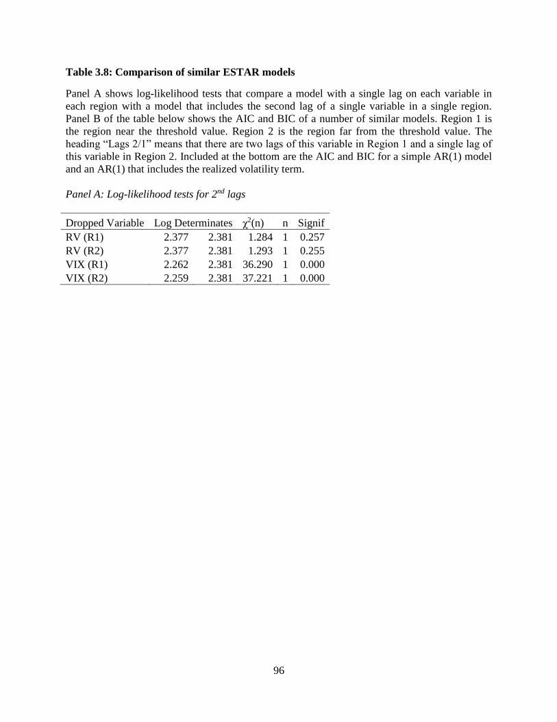
96
Table 3.8: Comparison of similar ESTAR models
Panel A shows log-likelihood tests that compare a model with a single lag on each variable in
each region with a model that includes the second lag of a single variable in a single region.
Panel B of the table below shows the AIC and BIC of a number of similar models. Region 1 is
the region near the threshold value. Region 2 is the region far from the threshold value. The
heading “Lags 2/1” means that there are two lags of this variable in Region 1 and a single lag of
this variable in Region 2. Included at the bottom are the AIC and BIC for a simple AR(1) model
and an AR(1) that includes the realized volatility term.
Panel A: Log-likelihood tests for 2nd lags
Dropped Variable Log Determinates χ2(n) n Signif
RV (R1) 2.377 2.381 1.284 1 0.257
RV (R2) 2.377 2.381 1.293 1 0.255
VIX (R1) 2.262 2.381 36.290 1 0.000
VIX (R2) 2.259 2.381 37.221 1 0.000
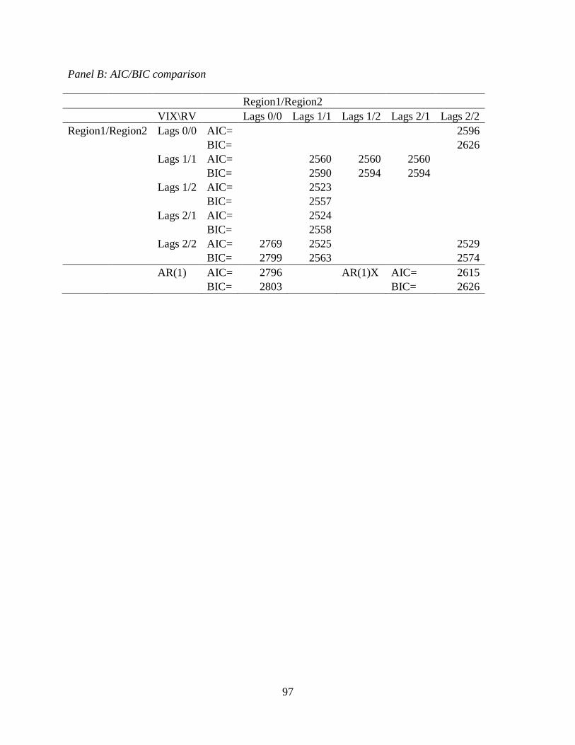
97
Panel B: AIC/BIC comparison
Region1/Region2
VIX\RV
Lags 0/0 Lags 1/1 Lags 1/2 Lags 2/1 Lags 2/2
Region1/Region2 Lags 0/0 AIC=
2596
BIC=
2626
Lags 1/1 AIC=
2560 2560 2560
BIC=
2590 2594 2594
Lags 1/2 AIC=
2523
BIC=
2557
Lags 2/1 AIC=
2524
BIC=
2558
Lags 2/2 AIC= 2769 2525
2529
BIC= 2799 2563
2574
AR(1) AIC= 2796
AR(1)X AIC= 2615
BIC= 2803
BIC= 2626
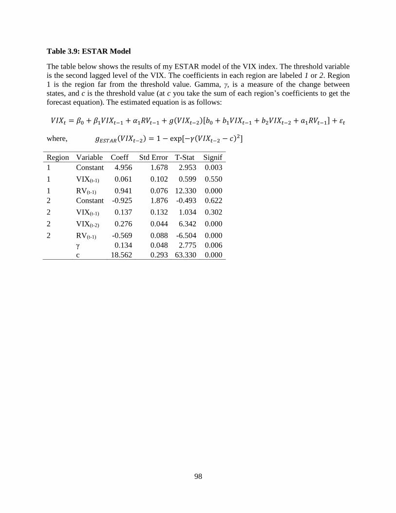
98
Table 3.9: ESTAR Model
The table below shows the results of my ESTAR model of the VIX index. The threshold variable
is the second lagged level of the VIX. The coefficients in each region are labeled 1 or 2. Region
1 is the region far from the threshold value. Gamma, γ, is a measure of the change between
states, and c is the threshold value (at c you take the sum of each region’s coefficients to get the
forecast equation). The estimated equation is as follows:
𝑉𝐼𝑋𝑡 = 𝛽0 + 𝛽1𝑉𝐼𝑋𝑡−1 + 𝛼1𝑅𝑉𝑡−1 + 𝑔(𝑉𝐼𝑋𝑡−2)[𝑏0 + 𝑏1𝑉𝐼𝑋𝑡−1 + 𝑏2𝑉𝐼𝑋𝑡−2 + 𝑎1𝑅𝑉𝑡−1] + 휀𝑡
where, 𝑔𝐸𝑆𝑇𝐴𝑅(𝑉𝐼𝑋𝑡−2) = 1 − exp[−𝛾(𝑉𝐼𝑋𝑡−2 − 𝑐)2]
Region Variable Coeff Std Error T-Stat Signif
1 Constant 4.956 1.678 2.953 0.003
1 VIX(t-1) 0.061 0.102 0.599 0.550
1 RV(t-1) 0.941 0.076 12.330 0.000
2 Constant -0.925 1.876 -0.493 0.622
2 VIX(t-1) 0.137 0.132 1.034 0.302
2 VIX(t-2) 0.276 0.044 6.342 0.000
2 RV(t-1) -0.569 0.088 -6.504 0.000
γ 0.134 0.048 2.775 0.006
c 18.562 0.293 63.330 0.000
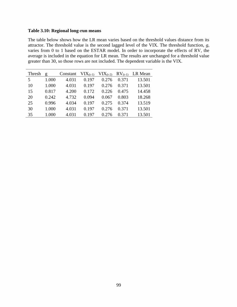
99
Table 3.10: Regional long-run means
The table below shows how the LR mean varies based on the threshold values distance from its
attractor. The threshold value is the second lagged level of the VIX. The threshold function, g,
varies from 0 to 1 based on the ESTAR model. In order to incorporate the effects of RV, the
average is included in the equation for LR mean. The results are unchanged for a threshold value
greater than 30, so those rows are not included. The dependent variable is the VIX.
Thresh g Constant VIX(t-1) VIX(t-2) RV(t-1) LR Mean
5 1.000 4.031 0.197 0.276 0.371 13.501
10 1.000 4.031 0.197 0.276 0.371 13.501
15 0.817 4.200 0.172 0.226 0.475 14.458
20 0.242 4.732 0.094 0.067 0.803 18.268
25 0.996 4.034 0.197 0.275 0.374 13.519
30 1.000 4.031 0.197 0.276 0.371 13.501
35 1.000 4.031 0.197 0.276 0.371 13.501
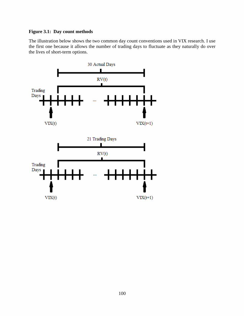
100
Figure 3.1: Day count methods
The illustration below shows the two common day count conventions used in VIX research. I use
the first one because it allows the number of trading days to fluctuate as they naturally do over
the lives of short-term options.
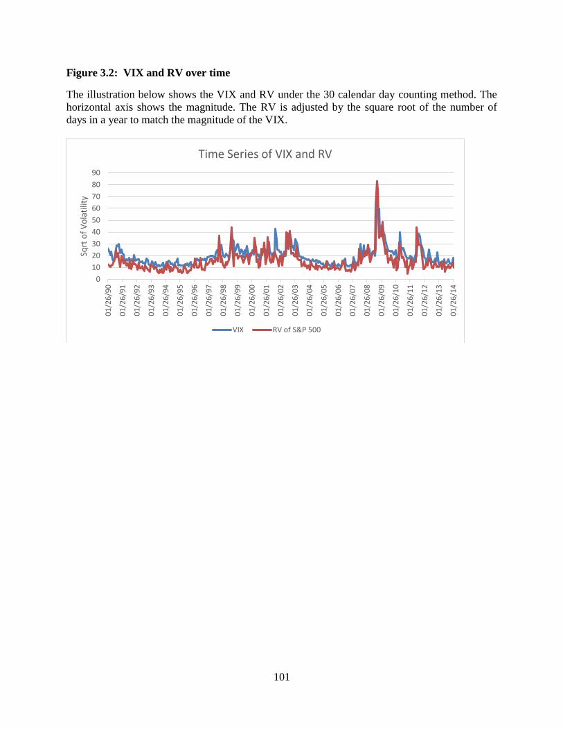
101
Figure 3.2: VIX and RV over time
The illustration below shows the VIX and RV under the 30 calendar day counting method. The
horizontal axis shows the magnitude. The RV is adjusted by the square root of the number of
days in a year to match the magnitude of the VIX.
0
10
20
30
40
50
60
70
80
90
01
/26
/90
01
/26
/91
01
/26
/92
01
/26
/93
01
/26
/94
01
/26
/95
01
/26
/96
01
/26
/97
01
/26
/98
01
/26
/99
01
/26
/00
01
/26
/01
01
/26
/02
01
/26
/03
01
/26
/04
01
/26
/05
01
/26
/06
01
/26
/07
01
/26
/08
01
/26
/09
01
/26
/10
01
/26
/11
01
/26
/12
01
/26
/13
01
/26
/14
Sqrt
of
Vo
lati
lity
Time Series of VIX and RV
VIX RV of S&P 500
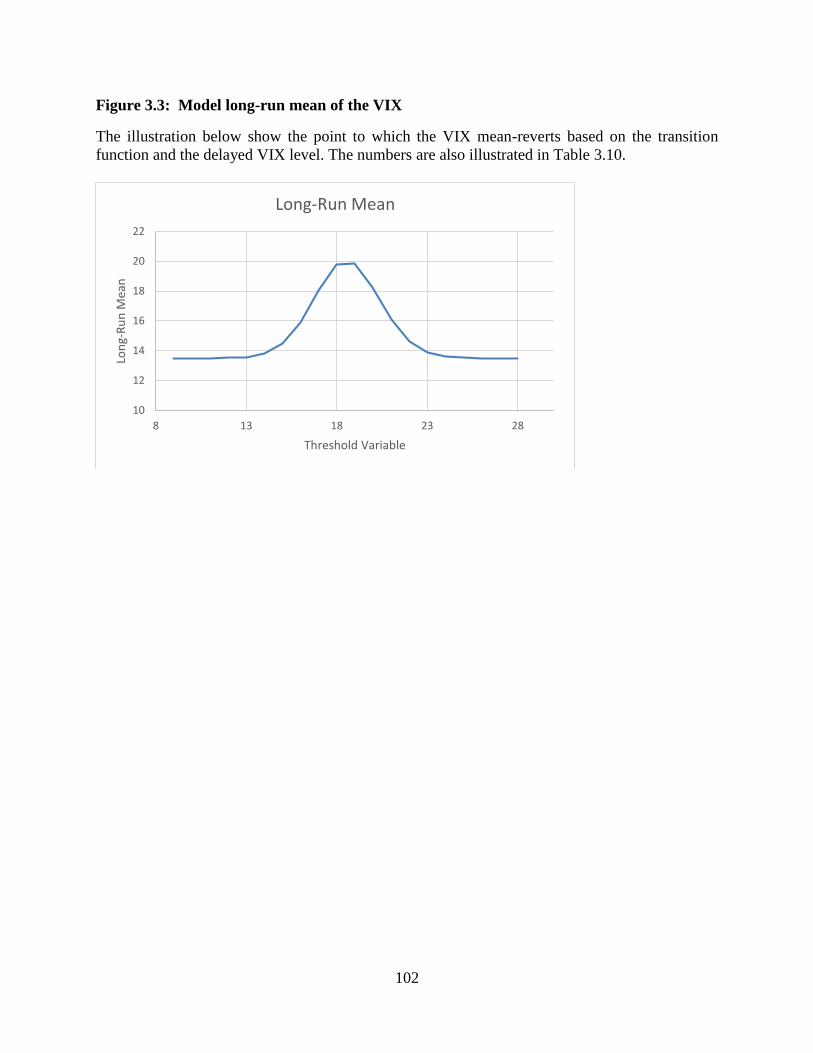
102
Figure 3.3: Model long-run mean of the VIX
The illustration below show the point to which the VIX mean-reverts based on the transition
function and the delayed VIX level. The numbers are also illustrated in Table 3.10.
10
12
14
16
18
20
22
8 13 18 23 28
Lon
g-R
un
Mea
n
Threshold Variable
Long-Run Mean
103
CHAPTER 4: PERFORMATIVITY-FREE OPTION PRICING MODEL RANKING
4.1. Introduction
Option pricing has developed an enormous literature over the past 50 years. One major
issue in derivatives pricing literature is that of performativity. Merriam-Webster’s Dictionary
defines performativity as follows: “being or relating to an expression that serves to effect a
transaction or that constitutes the performance of the specified act by virtue of its utterance.” As
models better capture the many eccentricities of financial markets, market prices tend to fit
models better. For example, when the Black-Scholes-Merton option pricing model first became
widely adopted by the market, it fit quite well because it was the model most traders used. If a
new model does actually fit the underlying better, empirical tests will be unlikely to agree
because the market itself is not using the new model. Since most OPMs have some form of
volatility term, the option price and the forward looking volatility are jointly unknown. Neither
can be directly computed without the other. To work around this issue, I propose a methodology
for ranking OPMs. A large number of OPMs use the normal distribution in some form because it
is tractable. OPMs also assume a specific stochastic process for the underlying. This
methodology is appropriate for OPMs that use some form of normal distribution and assume a
stochastic process for the underlying.
This chapter is organized as follows. Section 4.2 discusses the relevant literature. In
section 4.3, I introduce the three OPMs used in this paper and explain my new ranking

104
methodology. Section 3.4 gives the data sources. Section 4.5 discusses my empirical findings,
and section 4.6 presents the conclusions.
4.2. Literature Review
Our understanding of the nature of randomness predates almost all of modern science and
mathematics. The Roman philosopher, Lucretius (60 BC), gives one of the first known
descriptions of a mathematical process that has become known as Brownian motion. It is so
named for Robert Brown (1872) who observed the random movement of pollen particles.
Options trading has certainly been around for centuries. One of the first mathematically rigorous
papers on option pricing is Bachelier (1900) who developed an option pricing model based on
arithmetic Brownian motion, ABM. His line of inquiry lay dormant for decades until it was
“rediscovered” by Paul Samuelson in the 1950s.
Osborne (1959) did some of the earliest empirical work on the distributional
characteristics of stock prices. He uses the first and third quartiles of the distribution of stock
prices on a number of different days to establish the type of randomness in stock prices. He
concludes that geometric Brownian motion is the best fit. There are several issues with his use of
daily stock prices. There seems to be evidence that stock prices themselves are limited to a
particular range. I avoid this issue by using an index. His paper was groundbreaking in that it
expanded empirical testing methodologies to the stock market, but at the time there was some
controversy as to his actual contribution. In that same journal, Osborne (1962) expands upon his
initial approach by putting forward the log of the price relative as the best measure of the random
walk of stock prices. Interestingly, he also mentions that the outliers indicate a power distribution
with outliers playing a significant role in the overall process. Alexander (1961) also notes that

105
these “fat-tailed” distributions are a significant characteristic of economic statistics. This is
evidence against a normal distribution. Around this same time, there were a number of important
innovations on the theoretical side of option pricing.
Samuelson (1965) builds on several other earlier papers (including Sprenkle’s 1961
paper) that have used arithmetic and geometric Brownian motion. He lays out a number of
important boundary conditions for option pricing and even postulates that the direct equation for
a call price will be based on the heat equation in an appendix for his paper done by
mathematician Henry P. McKean, Jr. Concurrent with the aforementioned time period, Edward
Thorp and Sheen Kassouf (1967) began arbitraging the boundary conditions of warrants based
on their empirical observations. They both became wealthy and even published a book on their
system of trading in 1967. Samuelson and Merton (1969) use a utility framework to develop a
more generalized theory of warrant pricing. They also expand on the boundary conditions of
Samuelson’s previously mentioned paper. The reason that they resort to utility functions is that
they must use a general equilibrium model for pricing the warrant. Up until this time, there was
no profound agreement on the appropriate drift term or return on a particular stock, but there
should not be one because each individual’s required rate of return is intrinsic to their risk
preferences. This brings us to the remarkable innovations of Black, Scholes, and Merton.
There were three papers that have put forward the most ubiquitous OPM of our time. The
theoretical portion of the BSM OPM was put forward by Black and Scholes (1973). Sprenkle’s
(1961) model of warrants looks very similar to the BSM model except for the fact that the stock
price has an additional discount term k and the strike price is discounted by the term k*. Black
and Scholes note that researchers have not found an empirical solution to these terms. Black and
Scholes also borrow from Thorp and Kassouf who presented the idea of a hedge ratio. Using this

106
key observation, the heat transfer equation, and some difference equations they put forward their
iconic model. The only difference between their model and Sprenkle’s is that k = 1 and k* is
equal to the present value of $1 paid at expiration based on the risk-free rate. The big innovation
is that one only needs to know the risk-free rate not the appropriate required rate of return on the
stock. Merton (1973) expands on this model by simplifying it and re-deriving Black and Scholes’
difference equations in continuous time. He shows a proof of a continually rebalanced portfolio
and develops of the model’s underlying partial differential equation. In an interesting turn of fate
the empirical testing of the BSM model was published first.
Black and Scholes (1972) collected data on 2,039 calls and 3,052 straddles. They tested
their new model’s option pricing ability by comparing dollar returns on a hedged portfolio. They
also compare their model to market prices to see if trading on “overvalued” and “undervalued”
contracts leads to positive returns. They define “overvalued” as the market price being greater
than the model price. They do mention that if they trade based on their model, they lose a
significant amount of money each day. At this time option markets had not yet accepted the
BSM OPM15. The BSM OPM is based on geometric drift and geometric Brownian motion,
GBM. Since BSM, numerous extensions to their models have been formulated and tested.
As of the writing of this paper, SSRN lists over 2800 papers on option pricing. Much of
the empirical work seeks to find models that more closely match observed option prices. Some of
this has come in the form of allowing additional stochastic terms. Following many other
empirical investigations, Bakshi, Cao, and Chen (1997) develop an option pricing model that
uses stochastic volatility, stochastic interest rates, and stochastic jump processes. To test their
15 A more detailed history of the development of modern option pricing models can be found in
Chance (1995).
107
proposed model, they use observed option prices and compare them to their new models in three
ways: parameter consistency with observed data, out-of-sample pricing, and hedging.
Correspondingly, Carr and Wu (2004) propose a new framework for option pricing to address
jumps, stochastic volatility, and the leverage effect. To incorporate the leverage effect, their
model’s Brownian motion is negatively correlated with the Brownian motion driving their jump
process. In contrast to this approach, the ABM model address the leverage effect by assuming
that volatility remains unchanged even as the stock price decreases. This leads to price relative
volatilities that are negatively correlated with underlying returns.
Corsi, Fusari, and Vecchia (2013) propose an OPM that uses a long-memory stochastic
process in RV to proxy for unobserved option volatility. They test their model by using S&P 500
index futures and options. By estimating a stochastic drift term based on implied volatility, they
move their model closer to the standard normal distribution. Chambers, Foy, Liebner, and Lu
(2014) compare option models by computing historical option strategy returns. They then
compare these returns with returns derived from several well-known OPMs and show that for
out-of-the-money put options there seems to be a substantial premium. Here again the
methodology for comparing models uses option prices and underlying returns which introduces
performativity issues. Fulop, Li, and Yu (2015) develop a self-exciting model of return volatility
that includes Bayesian learning on the part of market participants. They use the S&P 500 index
to measure the effectiveness of their model. They find evidence that a single jump is likely to be
followed by other jumps as individuals adjust their beliefs about the underlying market. In
addition to more general OPMs that focus on stock prices, several researchers have proposed
particular models for certain underlyings.

108
The VIX is an index that measures overall market volatility by using the implied
volatilities in the equity options market. A literature has developed that seeks to predict stock
market volatility, and another literature looks at creating options on the VIX. Since it is often
used as a hedging instrument, it seems natural that investors would want to buy options on the
VIX. Wang and Daigler (2009) compare a number of different VIX option models. They find
that although a number of more complex models exist for modelling the VIX, the simpler models
perform better. They also mention some conversations with VIX options traders. These traders
use a BSM-style model instead of the more sophisticated models available. Mencía and Sentana
(2013) compare a number of different stochastic volatility models for the VIX. They use futures
and options over a number of time periods surrounding the recent financial crisis. They note that
there is a significant risk premium in the long-run volatility level. Their preferred model uses the
log of the VIX and incorporates stochastic volatility and mean reversion. This model is similar to
the CIR model tested below.
OPMs generally use the current price of the underlying, a current risk-free rate, the time-
to-maturity, the strike price, and a volatility term, but there are some complicating issues when it
comes to testing OPMs. The time to maturity and strike price are defined within the option
contract. The current underlying price and the risk-free rate can be observed in the marketplace.
The volatility is not and cannot be known with certainty. If the price is given, then volatility can
be solved for, or if the volatility is assumed, an option price can be computed. In the empirical
literature on option pricing, models are generally compared against the observed option prices.
Here I present a new method for ranking OPMs that circumvents this problem by relying
exclusively on the time series realizations of the underlying.

109
4.3. Methodology
There are an ever increasing number of stochastic processes that are commonly used in
option pricing. My goal is to simply compare several basic OPMs that are used for stock prices
and the VIX. By discretizing these stochastic processes, I get a simple approach that can be used
with almost any stochastic process. It turns out that discretization and numerical methods are
being used more and more often. Chen, Härkönen, and Newton (2014) demonstrate the use of
numerical integration to solve for a number of particularly intractable financial derivatives. To
provide a background, I will begin by briefly covering the several simple call option models and
their assumptions.
4.3.1. Black-Scholes-Merton option pricing model
The seminal papers of Black and Scholes (1973) and Merton (1973) put forward the
classic option pricing formula that bears their name. Writing their model in a way that
incorporates dividends, I get:
𝐶 = 𝑒−𝑟𝑇[𝑆0𝑒(𝑟−𝑞)𝑇𝑁(𝑑1) − 𝐾𝑁(𝑑2)]
where
𝑑1 =ln(𝑆0𝑒(𝑟−𝑞)𝑇 𝐾⁄ ) + 𝜎𝑔
2𝑇 2⁄
𝜎𝑔√𝑇
𝑑2 = 𝑑1 − 𝜎𝑔√𝑇
Here C is the call price, r is the risk-free rate, N(·) is the standard normal cumulative distribution
function, q is the dividend yield, T is the time to maturity, S0 is the current stock price, K is the
strike price, and σg is the annualized volatility defined in percentage terms. This model uses a
stochastic process of stock prices that can be written as follows:
𝑑𝑆 = 𝜇𝑔𝑆0𝑑𝑡 + 𝜎𝑔𝑆0𝑑𝑧

110
The stochastic process contains the volatility term and the drift term, μg. Here, the change in the
stock price follows some drift which can incorporate a dividend yield. The Wiener Process, dz, is
scaled by some relative volatility term and the current stock price. The distribution of the error
terms follows a log-normal distribution. One assumption of this model is that the stock price can
never be zero. Given limited liability, it follows that a stock price cannot be negative. However,
each year there is a small, but significant portion of the stock market that becomes totally
worthless through bankruptcy. The above model makes no allowance for this because under a
log-normal distribution, the price can never be zero. The drift term also has some curious
behavior.
The drift term is usually remapped to the risk-neutral world through the Radon-Nikodym
Derivative. Typically, the drift term is positive under the physical measure, but there are some
cases where a negative term is more appropriate (like derivatives based on the VIX). I next look
at a more recent model that is designed to be useful in the situations where the BSM OPM does
not work well.
4.3.2. Brooks-Brooks option pricing model
The recent paper of Brooks and Brooks (2013) pairs the properties of geometric drift with
arithmetic Brownian motion. Without geometric drift OPMs will be nonsensical because the drift
should increase with the price. There are several simple ways to exploit a process that does not
meet this process. Using the PDE, Brooks and Brooks find the following model for a call
option’s price under ABM:
𝐶 = 𝑒−𝑟𝑇[[𝑆0𝑒(𝑟−𝑞)𝑇 − 𝐾]𝑁(𝑑3) + 𝜎𝑎𝑛(𝑑3)]
where
𝑑3 =𝑆0𝑒𝑟𝑇 − 𝐾
𝜎𝑎
111
The volatility term, σa, is defined in absolute terms instead of percentage terms. Here the
stochastic process for the model can be written as follows:
𝑑𝑆 = 𝜇𝑎𝑆0𝑑𝑡 + 𝜎𝑎𝑑𝑧
The drift, μa, matches the previous BSM OPM, but will likely be different given the different
properties of the noise term. It is also important to note that the drift term is in dollar units not in
percentage units as in the BSM OPM. This model allows for a negative stock price, but the
boundary conditions are no longer violated when you include a zero strike put to include the
effects of limited liability.
4.3.3. Cox-Ingersoll-Ross model
The Cox-Ingersoll-Ross, CIR, model extends the Vasicek model by adding a volatility
term that depends on the underlying variable. It was originally used to model interest rates, and
Grünbichler and Longstaff (1996) use it to model the instantaneous behavior of the VIX. The
stochastic differential equation can be written as follows:
𝑑𝑉 = (𝛼 − 𝛽𝑉)𝑑𝑡 + 𝜎𝐶√𝑉𝑑𝑧
Here V is the underlying, α is some unknown parameter related to the long-run mean, β is the
speed of reversion towards this long-run level, and σc is the volatility term. Although incorrectly
specified for stock price movements, this model has gained popularity because it can be used to
model a number of mean-reverting variables that have increasing volatility in levels. The VIX
model presented by Grünbichler and Longstaff (1996) can be written as follows:
𝐶 = 𝑒−𝑟𝑇[𝑒−𝛽𝑇𝑉0𝑄(𝛾𝐾|𝜈 + 4, 𝜆) + (𝛼 𝛽⁄ )(1 − 𝑒−𝛽𝑇)𝑄(𝛾𝐾|𝜈 + 2, 𝜆) − 𝐾𝑄(𝛾𝐾|𝜈, 𝜆)]
where,
𝛾 =4𝛽
𝜎2(1 − 𝑒−𝛽𝑇) ,

112
𝜈 =4𝛼
𝜎2 ,
𝜆 = 𝛾𝑒−𝛽𝑇𝑉0
Here Q(·|ν + I, λ) is one minus the cumulative distribution function of a chi-squared distribution
with · as the random variable given (ν + I) degrees of freedom. The V0 is the initial price of the
underlying. The non-centrality parameter is represented by λ. They note that there is another
solution to this equation proposed by Sankaran (1963) that uses the normal distribution. This
model is also very similar in form to a previous model for the valuing options on yields by
Longstaff (1990).
4.3.4. Empirical testing
There is no way to observe a terminal distribution in markets. The market data we see is
only the realization of a near infinite number of random variables. As with many economic
questions, you cannot run a finely tuned series of experiments to create a terminal distribution to
test. A Monte Carlo style approach would simply confirm whichever model I put forward or use
to program the simulation. What we do have is a series of realized prices for the underlying.
With each of the above models the Weiner Process is the same, but it is scaled in different ways
with the underlying and different drift terms. A Weiner Process is equal to zero initially or is
equal to zero when no time has elapsed. It is also everywhere continuous and nowhere
differentiable. Additionally, it has the following property:
𝑊𝑡+∆𝑡 − 𝑊𝑡 ~ 𝑁(0, ∆𝑡)
Here N(0,Δt) is the normal distribution with a mean of zero and variance of Δt. The above
relationship holds for any t such that no matter where you start the variation is independent of
other time steps. I use daily data and constant time steps. Once I remove the effects of the drift
term and the terms that scale dz, I am left with a series of normally distributed error terms.

113
My method is formalized as follows: discretize each of the stochastic processes so that
the error terms are described only by a Weiner process, run a linear regression to get the error
terms, adjust the error terms for time and missing data effects, test the normality of each series,
and compare their distance to a normal distribution. Each of these steps has some assumptions
about the series and possible errors so I will describe each step in detail then give examples using
each of OPMs presented above.
All of the stochastic processes described above have a corresponding difference equation.
Writing the equation out is simple, but the coefficients are unknown. There is also an argument
that these coefficients cannot be known in the physical space. In its simplest form the drift term,
μ, and the volatility term, σ, are assumed to be constant. The drift term is based on an
unobservable risk premium so through the Girsanov Theorem the drift term is converted to the
risk-free rate. I do not change the measure; rather, I assume a constant drift term. This does not
mean that the drift term is always the same. As I note later on, options generally trade for
maturities of less than a year. Frequently, these derivatives have a maturity of around one month.
I assume that the drift term and volatility term are constant over a month. It is possible to use a
risk-free rate, but one which is appropriate. It is also possible to use some type of regression to
calculate daily or weekly risk premium, but any one of these adjustments will give a higher
variance than simply assuming a constant found with a linear regression. In order to get the
Weiner process as the last term, I use some algebra before or after discretization. Another
equally workable approach is to use the conditional distribution to project the current underlying
price one additional period forward. Both of these methods are illustrated below.
The next step is to calculate the coefficients through a regression. I use simple OLS.
Once the residuals are found they must be adjusted for differences in time steps. Here I use daily

114
data to calculate the series of error terms, but markets are not always open due to weekends and
holidays. To generalize volatility to any time-step, it is well-known that maturity dependent
volatility can be written as follows:
𝜎𝑇 = 𝜎√𝑇
I assume that trading day volatility is constant within each regression window. As a robustness
test later on, I count the days between observations and adjust the error terms accordingly. The
regression will yield error terms that can be written as follows:
�̂�𝑡 = 𝜎√𝑇휀𝑡
If all the time-steps were the same, the T term would have a simple scaling effect. Once the
error-terms are adjusted for missing values, they are tested for normality.
There are a number of tests for normality. Any of these will work in this methodology for
ranking OPMs. In the examples shown below, I use the Jarque-Bera test statistic. It uses the
skewness and kurtosis to test for normality. Another test that is useful in this context is the
Shapiro-Wilk test for normality. The Shapiro-Wilk test uses the difference between the ordered
sample terms and their order statistics to compare the series to the normal distribution. To
illustrate the initial step in this process I next show the discretization of each series.
The BSM OPM is based on the following stochastic process:
𝑑𝑆 = 𝜇𝑔𝑆0𝑑𝑡 + 𝜎𝑔𝑆0𝑑𝑧
To create a testable distribution I convert the above equation to a difference equation. For a
summary of the stochastic calculus involved, I would refer you to Mikosch (1999). The future
realization of the stock price under the above data generating process, DGP, is equal in
distribution to the following:
𝑆𝑡 =𝑑 𝑆𝑡−1𝑒𝑥𝑝 {(𝜇𝑔 −𝜎𝑔
2
2) ∆𝑡 + 𝜎𝑔√∆𝑡휀̃}

115
To create an empirical distribution of the stochastic term, I divide both sides by the initial stock
price and take the natural logarithm.
𝑙𝑛 (𝑆𝑡
𝑆𝑡−1) =𝑑 (𝜇𝑔 −
𝜎𝑔2
2) ∆𝑡 + 𝜎𝑔√∆𝑡휀̃
The BSM OPM assumes a constant risk-free rate and constant drift terms. The μ in the above
equation is not the risk-free rate but is a risk-adjusted return that is likely endogenously related to
the stock’s movements. The time intervals allow me to adjust for weekends and missing data
points. This simplifies the above equation to the following regression:
𝑙𝑛 (𝑆𝑡
𝑆𝑡−1) =𝑑 �̂�0∆𝑡 + √∆𝑡�̂�𝑔
By subtracting the estimated coefficient from the log of the price relative, I get a distribution of
error terms that, once adjusted for the time step, can be used for normality tests. Demeaning is
not necessary for testing the normality of the GBM distribution, but this setup matches well with
the ABM setup.
The ABM OPM is based on the following stochastic process:
𝑑𝑆 = 𝜇𝑎𝑆0𝑑𝑡 + 𝜎𝑎𝑑𝑧
The well-known conditional distribution for the above equation is shown below:
𝑆𝑡 =𝑑 𝑆𝑡−1𝑒𝑥𝑝(𝜇𝑎∆𝑡) + 𝜎𝑎√𝑒𝑥𝑝(2𝜇𝑎∆𝑡) − 1
2𝜇𝑎휀̃
Inserting constants as done previously gives,
𝑆𝑡 =𝑑 𝑆𝑡−1(𝑐0 + 1)∆𝑡 + 𝑐1√∆𝑡휀̃
Since the above equation has a constant of zero, we can use the first difference to put the above
equation in terms of returns. Rewriting gives the following regression,
∆𝑆𝑡 =𝑑 𝑆𝑡−1�̂�0∆𝑡 + √∆𝑡�̂�𝑎

116
The coefficient c0 is the same as simple return on the stock price for the given change in time.
Here the error term must be adjusted for the time step in the same way as the previous model.
The CIR model’s stochastic differential equation can be written as shown above:
𝑑𝑆 = 𝑎(𝑏 − 𝑆0)𝑑𝑡 + 𝜎𝑔√𝑆0𝑑𝑧
The CIR model can be discretized into the following well-known equation:
∆𝑆𝑡
√𝑆𝑡−1
=�̂��̂�∆𝑡
√𝑆𝑡−1
− �̂�√𝑆𝑡−1∆𝑡 + √∆𝑡�̂�𝑐
This setup allows once again for a simple linear regression to obtain the series of error
terms. The series of errors is then adjusted for different time steps to give the testable
distribution. The error terms for ABM, GBM, and CIR can be compared to test which one is a
better fit for option pricing.
Each of the presented OPMs has used properties of the normal distribution to give a
tractable model. The question of which model is a better fit for stock prices or any underlying
remains. I test each series of time-step corrected error terms for normality using the Jarque-Bera
Test. This test statistic is defined for use with regressions as follows:
𝐽𝐵 =𝑛 − 𝑘
6(𝑆𝑘2 +
1
4(𝐾𝑢 − 3)2)
Where, n is the number of observations, k is the number of regressors, Sk is the skewness of the
error terms, and Ku is the kurtosis of the error terms. The above statistic is compared to a χ2
distribution with two degrees of freedom16. If the given error terms are normal then they should
have a skewness equal to 0 and kurtosis equal to 3. It is highly unexpected to fail to reject the
null hypothesis of normality in any of our empirical setups because it is well known that stock
16 In small samples this is test has a high Type-I error rate. A table of p-value conversions is
available for hypothesis testing, but this is not the way that I use the test.

117
returns are negatively skewed and leptokurtic. Here the test statistic is used to measure which
model is closer to normal. Other methods will work equally as well to test normality of these
error terms.
4.4. Data
There are two data sets that I use to test this methodology: the S&P 500 and the VIX. For
the S&P 500, I use the daily closing prices without dividends. Dividends are not included in
option pricing unless an extraordinarily high dividend is paid. These closing prices are readily
available online from a large number of sources. The S&P 500 is an index based on the stock
price of just over 500 companies that are representative of major US industries. These companies
are chosen by committee and are also subject to several liquidity constraints. This index is a
widely-used measure of the US economy and the stock market as a whole.
The VIX is an index designed to track market volatility. It was originally based on the
S&P 100, but was redesigned to better match market conditions in 2003 (for a more detailed
explanation of this change see Whaley, 2009). The VIX in its current incarnation is the square
root of the fixed leg of a 30-day variance swap. The fixed leg of this swap is implied by a
number of implied volatilities in the options market. Since these options generally expire on the
third week of each month, the implied volatilities of the nearby and second nearby options are
used to build a term structure of volatility. This term structure is then used to compute the swap
price or fixed leg. The methodology for obtaining the VIX has been applied to historical data so
that the dataset begins before the new method for computing it was put forward. The daily VIX
data must be adjusted because it has an overlapping data issue.
118
The options used to compute the VIX are within 39 days of their expiration. Since the
method to compute the VIX uses a weighted average of the nearby and second nearby, using
daily data will introduce an enormous amount of false serial correlation into the data set. To
remedy this issue, I follow the 30-day calendar method put forward in Adhikari and Hillard
(2014). So, for my analysis the distance between any two observations is at least 30 calendar
days. Both data sets are included in the summary statistics shown in Table 4.1, Figure 4.1, and
Figure 4.2. The summary statistics show many commonly known attributes of financial market
data. The S&P 500 has a significant level of serial correlation which is consistent with the unit-
root often found in stock market data. The averages are only important for the VIX series which
tends to be mean-reverting. Once the 30 day count method is used, the serial correlation drops
noticeably.
4.5. Empirical findings
There is a wide range of applications for this testing methodology. It circumvents a major
issue in empirical option pricing literature. The results from applying this methodology to the
S&P 500 and the VIX are shown below.
4.5.1. S&P 500 testing
The S&P 500 is an index of many major stock prices. Although the CIR model is not
appropriate given its mean-reverting assumptions, I use it for illustrative purposes in testing the
S&P 500. I begin by using the entire series of data points in a single regression to get my
residuals. I will later add the monthly regression results. The results from my tests without
counting the extra time from weekends and missing days are shown in Table 4.2 and illustrated
in Figures 4.3 and 4.4. A lower Jarque-Bera Test statistic indicates that the error terms are closer

119
to the mean. As can be seen from the table above, the ABM model fits best. It is followed by the
CIR model, and the GBM model has the worst fit of the three models. Many of these differences
come from the kurtosis of each residual series. Although each series displays negative skewness,
the GBM model has a much higher level of kurtosis than the other models. This is due to the way
that the natural logarithm reshapes the distribution of error terms.
4.5.2. VIX testing
The 30 day count VIX data is tested using my methodology. The results shown in Table
4.3 indicate that the best fit is the GBM model. Econometrically, the Grünbichler and Longstaff
(1996) model gives the best setup to capture the empirically observed behaviors of the VIX. The
VIX is and must be mean-reverting because it is based on the standard deviation of an index. It is
sometimes termed the “fear index” because during times of economic turmoil it spikes to
significant heights. The CIR model accurately captures both of these characteristics. It allows for
mean-reversion through the drift term and scales the volatility so that the distribution is right
skewed. However, the GBM model still fits best. This is consistent with Wang and Daigler
(2009), who in empirical testing note that the Grünbichler and Longstaff model gives systematic
errors when compared to observed option prices. They also note that traders in VIX options tend
to use a form of the BSM model. My results reinforce the BSM model as the best fit for the VIX.
4.6. Conclusions
The preceding pages put forward a new empirical method for ranking OPMs. This
method does not use the option prices observed in the market and is thus free from the common
performativity problem in finance. Performativity is often an issue for economics and finance
researchers because the whole market can be wrong about a model, but if they are all in

120
agreement, then new or better models will not show empirical value until they are widely
implemented by the market. The methodology presented here makes several assumptions about
an OPMs drift terms and uses the properties of Brownian motion to create a testable vector of
error terms which can be compared by their distance to the normal distribution.
I have shown that in my initial testing of these models, the BSM OPM is the best fit for
options that use the VIX as the underlying. This is consistent with previous papers on VIX
option pricing. The ABM model is the best fit for the S&P 500 index. This is consistent with
Brooks and Brooks (2013) who put forward a new option pricing model that allows for stocks to
become worthless. Going forward, I intend to use a number of common option maturity windows
and use a rolling regression approach to see how this methodology matches different classes of
underlying securities with different classes of OPMs.
121
REFERENCES
Adhikari, B. & Hilliard, J. (2014). The VIX, VXO and realized volatility: a test of lagged and
contemporaneous relationships. International Journal of Financial Markets and Derivatives 3,
222-240.
Alexander, S.S. (1964). Price movements in speculative markets: trends or random walks, No. 2.
In Cootner, P.H., ed., 1964. The Random Character of Stock Market Prices. The M.I.T. Press,
Cambridge, MA, 338-375.
Bachelier, L. (1900). Théorie de la Spéculation. Annales de l’Ecole Normale Superieure 17 (3),
No. 1018 (Paris, Gauthier-Villars). Thesis at Academy of Paris, March 29, 1900. Translated by J.
Boness in Cootner, P., 1964. The Random Character of Stock Market Prices (Cambridge, MA:
MIT Press), 17-78.
Bakshi, G., Cao, C., & Chen, Z. (1997). Empirical performance of alternative option pricing
models. The Journal of Finance 52, 2003-2049.
Black, F. & Scholes, M. (1973). The pricing of options and corporate liabilities. Journal of
Political Economy 81, 637-659.
Black, F. & Scholes, M. (1972). The valuation of option contracts and a test of market efficiency.
The Journal of Finance 27, 399-417.
Brooks, R. & Brooks, J. (2013). Another look at option valuation based on arithmetic Brownian
motion. Unpublished working paper. The University of Alabama.
Carr, P. & Wu, L. (2004). Time-changed Lévy processes and option pricing. Journal of Financial
Economics 71, 113-141.
Chambers, D., Foy, M., Liebner, J., & Lu, Q. (2014). Index option returns: still puzzling. The
Review of Financial Studies 27, 1915-1928.
Chance, D.M. (1995). A chronology of derivatives. Derivatives Quarterly, 53-60.
Chen, D., Härkönen, H., & Newton, D. (2014). Advancing the universality of quadrature
methods to any underlying process for option pricing. Journal of Financial Economics 114, 600-
612.

122
Corsi, F., Fusari, N., & Vecchia, D. (2013). Realizing smiles: options pricing with realized
volatility. Journal of Financial Economics 107, 284-304.
Cox, J.C., Ingersoll, J.E., & Ross, S.A. (1985). A theory of the term structure of interest rates.
Econometrica 53, 385-408.
Fulop, A., Li, J., & Yu, J. (2015). Self-exciting jumps, learning, and asset pricing implications.
The Review of Financial Studies 28, 876-912.
Grünbichler, A. & Longstaff, F. (1996). Valuing futures and options on volatility. Journal of
Banking & Finance 20, 985-1001.
Kassouf, S. & Thorp, E. (1967). Beat the Market: A Scientific Stock Market System. Random
House, New York.
Longstaff, F. (1990). The valuation of options on yields. Journal of Fianncial Economics 26, 97-
121.
Lucretius, T.C. (60 BC). De rerum natura (On the Nature of Things).
Mencía, J. & Sentana, E. (2013). Valuation of VIX derivatives. Journal of Financial Economics
108, 367-391.
Merton, R. (1973). Theory of rational option pricing. Bell Journal of Economics and
Management Science 4, 141-183.
Mikosch, T. (1999). Elementary stochastic calculus with finance in view. In: Barndorff-Nielsen,
O.E., (Ed.), Advanced Series on Statistical Science and Applied Probability, Vol. 6. World
Scientific, Singapore.
Osborne, M. (1959). Brownian motion in the stock market. Operations Research 7, 143-173.
Osborne, M. (1962). Periodic structure in the Brownian motion of stock prices. Operations
Research 10, 345-379.
Samuelson, P., (1965). Rational theory of warrant pricing. Industrial Management Review 6, 13-
39.
Samuelson, P. & Merton, R. (1969). A complete model of warrant pricing that maximizes utility.
Industrial Management Review 10, 17-46.
Sankaran, M. (1963). Approximations to the non-central chi-squared distribution. Biometrika 50,
199-204.

123
Sprenkle, C. (1961). Warrant prices as indicators of expectations and preferences. Yale
Economic Essays 1, 178-231. In Cootner, P., ed., 1964. The Random Character of Stock Market
Prices. The M.I.T. Press, Cambridge, MA, 412-474.
Wang, Z. & Daigler, R. (2009). The performance of VIX option pricing models: empirical
evidence beyond simulation. Unpublished working paper. Florida International University.
Whaley, R. (1993). Derivatives on market volatility. The Journal of Derivatives 1, 71-84.
Whaley, R. (2009). Understanding the VIX. Journal of Portfolio Management 35, 98-105.
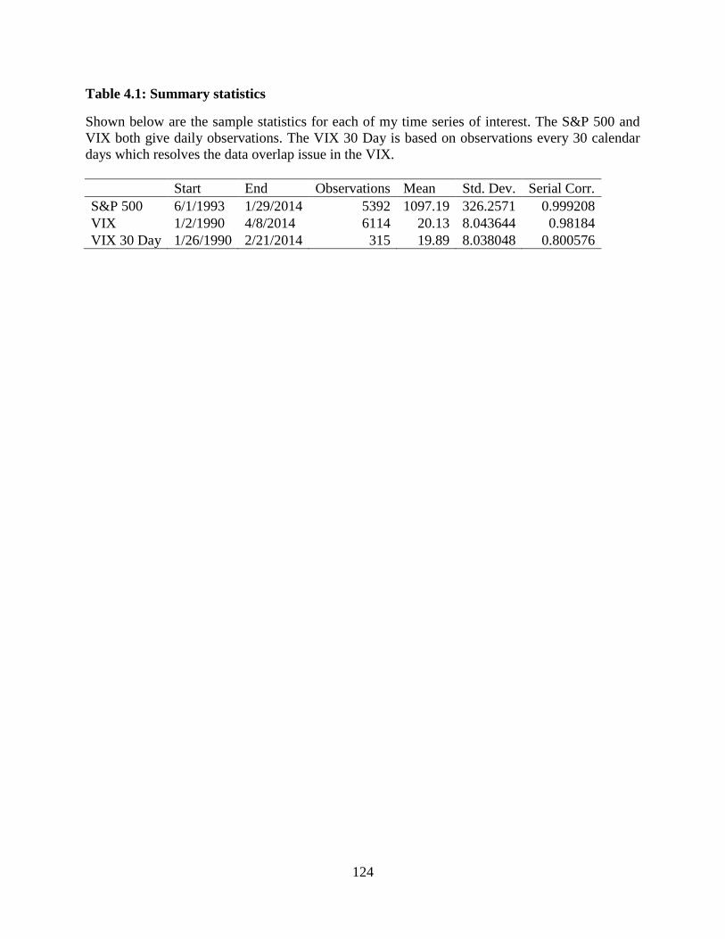
124
Table 4.1: Summary statistics
Shown below are the sample statistics for each of my time series of interest. The S&P 500 and
VIX both give daily observations. The VIX 30 Day is based on observations every 30 calendar
days which resolves the data overlap issue in the VIX.
Start End Observations Mean Std. Dev. Serial Corr.
S&P 500 6/1/1993 1/29/2014 5392 1097.19 326.2571 0.999208
VIX 1/2/1990 4/8/2014 6114 20.13 8.043644 0.98184
VIX 30 Day 1/26/1990 2/21/2014 315 19.89 8.038048 0.800576
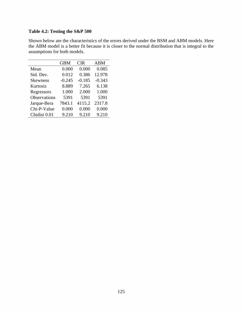
125
Table 4.2: Testing the S&P 500
Shown below are the characteristics of the errors derived under the BSM and ABM models. Here
the ABM model is a better fit because it is closer to the normal distribution that is integral to the
assumptions for both models.
GBM CIR ABM
Mean 0.000 0.000 0.085
Std. Dev. 0.012 0.386 12.978
Skewness -0.245 -0.185 -0.343
Kurtosis 8.889 7.265 6.138
Regressors 1.000 2.000 1.000
Observations 5391 5391 5391
Jarque-Bera 7843.1 4115.2 2317.8
Chi-P-Value 0.000 0.000 0.000
Chidist 0.01 9.210 9.210 9.210
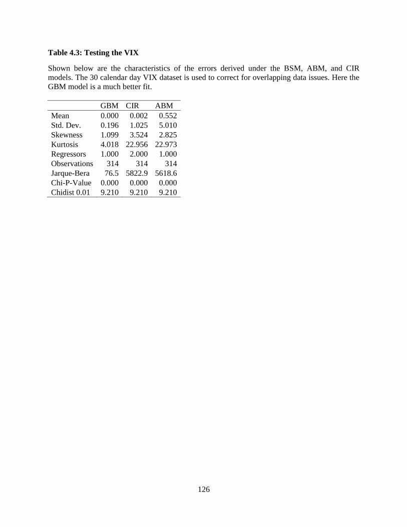
126
Table 4.3: Testing the VIX
Shown below are the characteristics of the errors derived under the BSM, ABM, and CIR
models. The 30 calendar day VIX dataset is used to correct for overlapping data issues. Here the
GBM model is a much better fit.
GBM CIR ABM
Mean 0.000 0.002 0.552
Std. Dev. 0.196 1.025 5.010
Skewness 1.099 3.524 2.825
Kurtosis 4.018 22.956 22.973
Regressors 1.000 2.000 1.000
Observations 314 314 314
Jarque-Bera 76.5 5822.9 5618.6
Chi-P-Value 0.000 0.000 0.000
Chidist 0.01 9.210 9.210 9.210
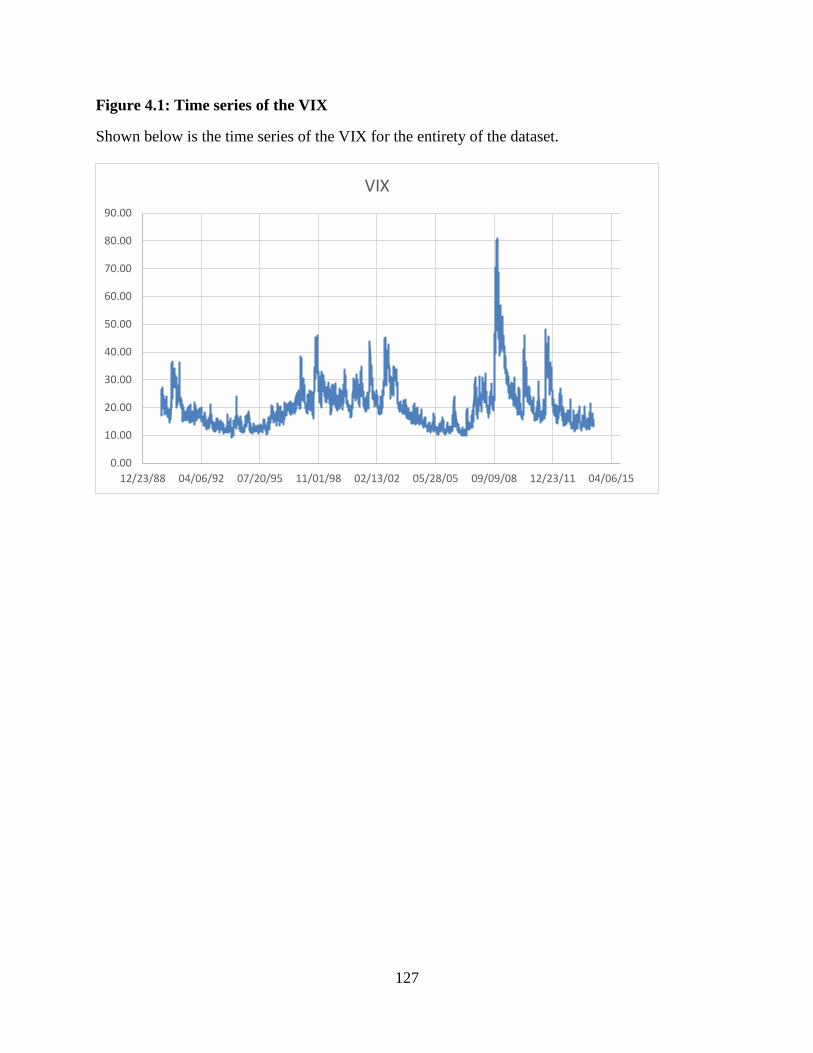
127
Figure 4.1: Time series of the VIX
Shown below is the time series of the VIX for the entirety of the dataset.
0.00
10.00
20.00
30.00
40.00
50.00
60.00
70.00
80.00
90.00
12/23/88 04/06/92 07/20/95 11/01/98 02/13/02 05/28/05 09/09/08 12/23/11 04/06/15
VIX
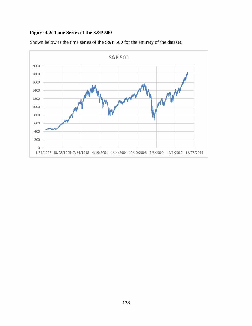
128
Figure 4.2: Time Series of the S&P 500
Shown below is the time series of the S&P 500 for the entirety of the dataset.
0
200
400
600
800
1000
1200
1400
1600
1800
2000
1/31/1993 10/28/1995 7/24/1998 4/19/2001 1/14/2004 10/10/2006 7/6/2009 4/1/2012 12/27/2014
S&P 500
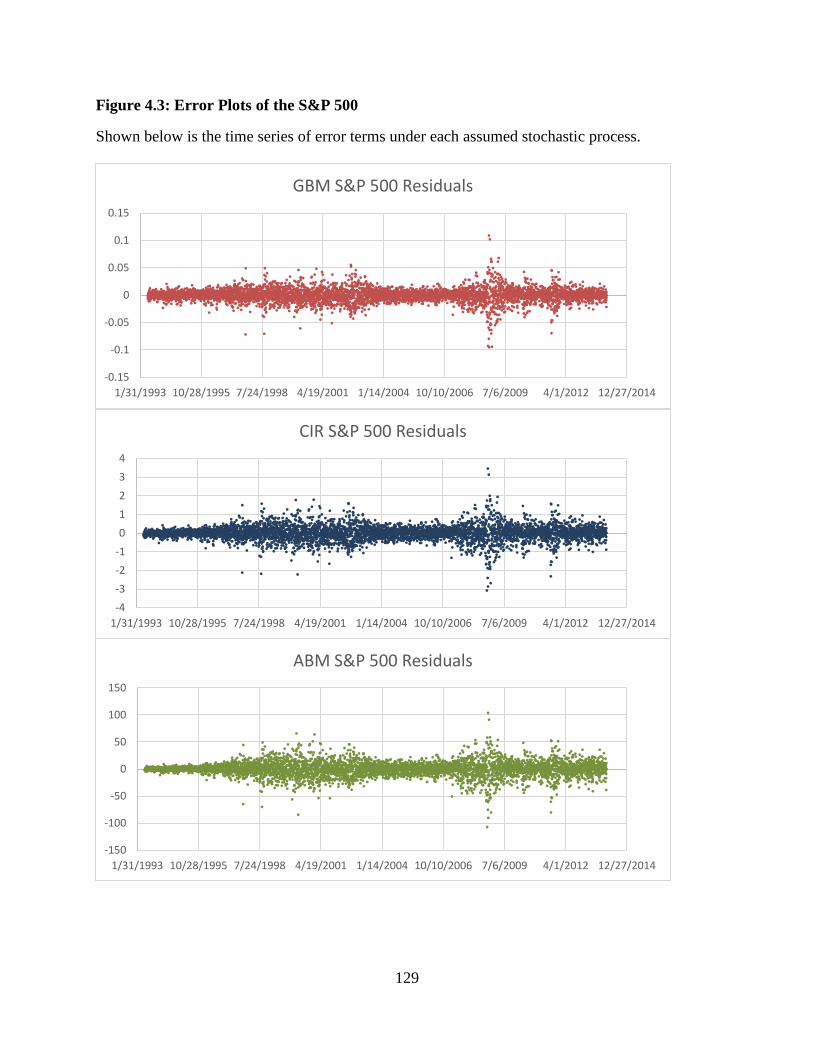
129
Figure 4.3: Error Plots of the S&P 500
Shown below is the time series of error terms under each assumed stochastic process.
-0.15
-0.1
-0.05
0
0.05
0.1
0.15
1/31/1993 10/28/1995 7/24/1998 4/19/2001 1/14/2004 10/10/2006 7/6/2009 4/1/2012 12/27/2014
GBM S&P 500 Residuals
-4
-3
-2
-1
0
1
2
3
4
1/31/1993 10/28/1995 7/24/1998 4/19/2001 1/14/2004 10/10/2006 7/6/2009 4/1/2012 12/27/2014
CIR S&P 500 Residuals
-150
-100
-50
0
50
100
150
1/31/1993 10/28/1995 7/24/1998 4/19/2001 1/14/2004 10/10/2006 7/6/2009 4/1/2012 12/27/2014
ABM S&P 500 Residuals
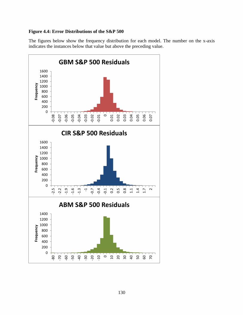
130
Figure 4.4: Error Distributions of the S&P 500
The figures below show the frequency distribution for each model. The number on the x-axis
indicates the instances below that value but above the preceding value.
0
200
400
600
800
1000
1200
1400
1600
-0.0
8
-0.0
7
-0.0
6
-0.0
5
-0.0
4
-0.0
3
-0.0
2
-0.0
1 0
0.0
1
0.0
2
0.0
3
0.0
4
0.0
5
0.0
6
0.0
7
Fre
qu
en
cy
GBM S&P 500 Residuals
0
200
400
600
800
1000
1200
1400
1600
-2.5
-2.2
-1.9
-1.6
-1.3 -1
-0.7
-0.4
-0.1
0.2
0.5
0.8
1.1
1.4
1.7 2
Fre
qu
en
cy
CIR S&P 500 Residuals
0
200
400
600
800
1000
1200
1400
-80
-70
-60
-50
-40
-30
-20
-10 0
10
20
30
40
50
60
70
Fre
qu
en
cy
ABM S&P 500 Residuals
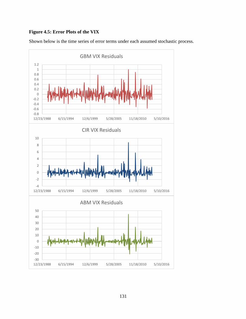
131
Figure 4.5: Error Plots of the VIX
Shown below is the time series of error terms under each assumed stochastic process.
-0.8
-0.6
-0.4
-0.2
0
0.2
0.4
0.6
0.8
1
1.2
12/23/1988 6/15/1994 12/6/1999 5/28/2005 11/18/2010 5/10/2016
GBM VIX Residuals
-4
-2
0
2
4
6
8
10
12/23/1988 6/15/1994 12/6/1999 5/28/2005 11/18/2010 5/10/2016
CIR VIX Residuals
-30
-20
-10
0
10
20
30
40
50
12/23/1988 6/15/1994 12/6/1999 5/28/2005 11/18/2010 5/10/2016
ABM VIX Residuals
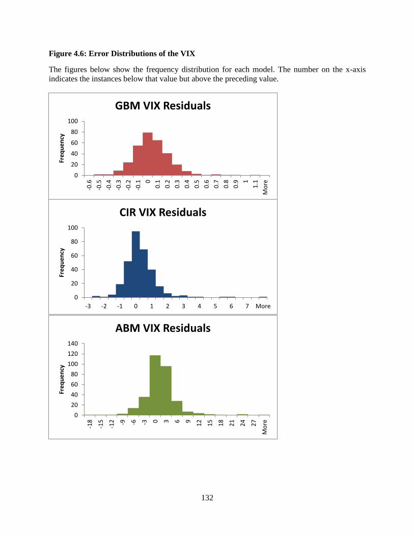
132
Figure 4.6: Error Distributions of the VIX
The figures below show the frequency distribution for each model. The number on the x-axis
indicates the instances below that value but above the preceding value.
0
20
40
60
80
100
-0.6
-0.5
-0.4
-0.3
-0.2
-0.1 0
0.1
0.2
0.3
0.4
0.5
0.6
0.7
0.8
0.9 1
1.1
Mo
re
Fre
qu
en
cy
GBM VIX Residuals
0
20
40
60
80
100
-3 -2 -1 0 1 2 3 4 5 6 7 More
Fre
qu
en
cy
CIR VIX Residuals
0
20
40
60
80
100
120
140
-18
-15
-12 -9 -6 -3 0 3 6 9
12
15
18
21
24
27
Mo
re
Fre
qu
en
cy
ABM VIX Residuals