Embed Size (px)
Citation preview
1
Three Monte Carlo programs of polarized light transport into scattering media: part I
Jessica C. Ramella-Roman, Scott A. Prahl, Steve L. Jacques
Johns Hopkins University Applied Physics Laboratory, Laurel MD, Oregon Medical Laser Center, Portland OR, Oregon Health & Science University, Portland, OR
[email protected], [email protected], [email protected]
Abstract: Propagation of light into scattering media is a complex problem that can be modeled using statistical methods such as Monte Carlo. Few Monte Carlo programs have so far included the information regarding the status of polarization of the photon before and after every scattering event. Different approaches have been followed and limited numerical values have been made available to the general public. In this paper, three different ways to build a Monte Carlo program for light propagation with polarization are given. Different groups have used the first two methods; the third method is original. Comparison in between Monte Carlo runs and Adding Doubling program yielded less than 1 % error. ©2005 Optical Society of America OCIScodes : (290.4020) Mie theory (290.4210) Multiple scattering
References and Links 1. S. Chandrasekhar, Radiative Transfer, Oxford Clarendon Press; (1950). 2. S. Chandrasekhar and D. Elbert, “The Illumination and polarization of the sunlight sky on Rayleigh
scattering,” Trans. Am. Phil. Soc., 44, 6, 1956. 3. K. F. Evans and G. L. Stephens, “A new polarized atmospheric radiative transfer model,” J. Quant.
Spectrosc. Radiat Transfer., 46, 5:413-423, 1991. 4. S. A. Prahl, M. J. C. van Gemert, A. J. Welch, “Determining the optical properties of turbid media by using
the adding-doubling method,” Applied Optics, 32:559-568, 1993. 5. G. W. Kattawar and G. N. Plass “Radiance and polarization of multiple scattered light from haze and
clouds,” Applied Optics, 7, 8:1519-1527, 1967. 6. G. W. Kattawar and G. N. Plass, “Degree and direction of polarization of multiple scattered light. 1:
Homogeneous cloud layers,” Applied Optics, 11, 12:2851-2865, 1972. 7. G. W. Kattawar and C. N. Adams “Stokes vector calculations of the submarine light field in an atmosphere-
ocean with scattering according to a Rayleigh phase matrix: effect of interface refractive index on radiance and polarization,” Limnol. Oceanogr., 34, 8:1453-1472, 1989.
8. P. Bruscaglione, G. Zaccanti, W. Qingnong “Transmission of a pulsed polarized light beam through thick turbid media: numerical results,” Applied Optics, 32, 30:6142-6150, 1993.
9. S. Bianchi, A. Ferrara, C. Giovannardi, “Monte Carlo simulations of dusty spiral galaxies: extinction and polarization properties,” American Astronomical Society, 465,1:137-144,1996.
10. S. Bianchi Estinzione e polarizzazione della radiazione nelle galassie a spirale, Tesi di Laura (in Italian), 1994.
11. A. Ambirajan and D.C. Look, “A backward Monte Carlo study of the multiple scattering of a polarized laser beam,” J. Quant. Spectrosc. Radiat. Transfer, 58, 2:171-192; 1997.
12. A. S. Martinez and R. Maynard “Polarization Statistics in Multiple Scattering of light: a Monte Carlo approach,” in Localization and Propagation of classical waves in random and periodic structures Plenum Publishing Corporation New York, 1993.
13. A. S. Martinez Statistique de polarization et effet Faraday en diffusion multiple de la lumiere Ph.D. Thesis (in French and English), 1984.
14. S. Bartel and A. Hielsher, “Monte Carlo simulations of the diffuse backscattering Mueller matrix for highly scattering media,” Applied Optics, 39, 10:1580:1588, 2000.
15. B. D. Cameron, M. J. Rakovic, M. Mehrubeoglu, G. Kattawar, S. Rastegar, L.-H. Wang, G. L. Cote, “Measurement and calculation of the two-dimensional backscattering Mueller matrix of a turbid medium,” Optics Letters, 23: 485-487, 1998.
16. M. J. Rakovic, G. W. Kattawar, M. Mehrubeoglu, B. D. Cameron, L.-H. Wang, S. Rastegar, G. L. Cote, “Light backscattering polarization patterns from turbid media: theory and experiment,” Applied Optics, 38:3399-3408, 1999.
2
17. Daniel Côté, I. Alex Vitkin “Robust concentration determination of optically active molecules in turbid media with validated three-dimensional polarization sensitive Monte Carlo calculations,” Optics Express, 13, 148-163, 2005.
18. N. Metropolis and S. Ulam, “The Monte Carlo method,” Journal of the American Statistical Association, 44:335-341, 1949.
19. S. A. Prahl, M. Keijzer, S. L. Jacques, A. J. Welch, “A Monte Carlo model of light propagation in tissue,” In Dosimetry of Laser Radiation in Medicine and Biology, G. Mueller, D. Sliney, Eds., SPIE Series 5: 102-111, 1989.
20. L. H Wang, S. L. Jacques, L-Q Zheng, “MCML – Monte Carlo modeling of photon transport in multi-layered tissues,” Computer Methods and Programs in Biomedicine, 47:131-146, 1995.
21. A. N. Witt, “Multiple scattering in reflection nebulae I: A Monte Carlo approach,” Astophys. J. Suppl. Ser., 35:1-6, 1977.
22. J. J. Craig, Introduction to robotics. Mechanics and controls, Addison-Weseley Publishing Company, 1986. 23. D. Benoit, D. Clary “Quaternion formulation of diffusion quantum Monte Carlo for the rotation of rigid
molecules in clusters,” Journal of chemical physics, 113, 12:5193-5202, 2000. 24. M. Richartz. and Y. Hsu, “Analysis of elliptical polarization,” J. Opt. Soc. Am. 39:136-157, 1949. 25. K. I. Hopcraft, P. C. Y. Chang, J. G. Walker, E. Jakeman, Properties of Polarized light-beam multiply
scattered by Rayleigh medium, F. Moreno and F. Gonzales (Eds.), Lectures 1998, Springer-Verlag, 534: 135-158, 2000.
26. W. H. Press, S. A. Teukolsky, W. T. Vetterling, B. P. Flannery, Numerical Recipes in C, the art of Scientific Computing, Cambridge University Press, 1992.
27. C. Bohren and D. R. Huffman, Absorption and scattering of light by small particles, Wiley Science Paperback Series,1998.
28. http://omlc.ogi.edu/software/mie/index.html 29. W. J. Wiscombe, “Improved Mie scattering algorithms,” Applied Optics, 19, 9:1505-1509, 1980. 30. J. W. Hovenier, “Symmetry Relationships for Scattering of Polarized Light in a Slab of Randomly Oriented
Particles,” Journal of the Atmospheric Sciences, 26:488-499, 1968. 31. http://omlc.ogi.edu/software/polarization/ 32. J. B. Kuipers, Quaternions and rotation sequences. A primer with applications to orbits, aerospace, and
virtual reality Princeton University Press, 1998 33. K. Shoemake, “Animating rotation with quaternion curves,” Computer Graphics 19, 3:245-254, 1985. 34. J.C. Ramella-Roman, S.A.Prahl, S.L. Jacques, “Three Monte Carlo programs of polarized light transport
into scattering media: part II,” Optics Express
1. Introduction
Over the last fifty years polarized light travel through scattering media has been studied by many groups and by the atmospheric optics and oceanography community in particular. An exact solution of the radiative transfer for a plane-parallel atmosphere with Rayleigh scattering was derived by Chandrasekhar in 1950 [1,2]. More complicated geometries proved too complex to be solved analytically. Adding-doubling methods were developed to handle the same kind of geometry for inhomogeneous atmosphere containing randomly oriented particles [3,4].
Kattawar and Plass [5] were the first to calculate the status of polarization of photons after multiple scattering using a Monte Carlo method. They later defined the degree of polarization for homogeneous layers for different solar zenith angles and optical thickness for haze and clouds [6]. Since then many papers have been published on Monte Carlo models and their applications. Kattawar and Adams used a Monte Carlo program to calculate the Stokes vector at any location in a fully inhomogeneous atmosphere-ocean system [7]. Other groups used Monte Carlo codes to analyze changes in polarization of light pulses transmitted through turbid media [8]. Monte Carlo programs were used to measure the polarization properties of dusty spiral galaxies by Bianchi et al. [9,10]; a detailed description of their Monte Carlo program was included. Ambirajan and Look [11] developed a backward Monte Carlo model for slab geometry with circularly polarized incident light. Martinez and Maynard [12] wrote a Monte Carlo program for the plane slab geometry and used it to study the Faraday-effect in an optically active medium [13].
Bartel and Hielsher [14] proposed a Monte Carlo model that differs from previous programs that used a local coordinate system to keep track of the polarization reference frame; the coordinate system is rotated with standard rotational matrices. They calculated the diffusely back-scattered Mueller Matrix for suspension of polystyrene spheres and their results where compared with experimental results. Cameron et al. showed similar images

3
both experimentally and numerically [15]. Finally Rakovic et al. [16] proposed a numerical method to simultaneously calculate all 16 elements of the two-dimensional Mueller matrix that compared favorably with their Monte Carlo program.
Unfortunately none of the Monte Carlo programs mentioned above were made freely available to the scientific community. Recently, Cote’ et al. released their polarized light Monte Carlo program [17]; they use two vectors to keep track of the polarization reference frame similarly to Bartel and Hielsher.
In this paper we want to illustrate three different way of implementing Monte Carlo programs that track the status of polarization of scattered photons as they propagate in solutions of Mie and Rayleigh scatterers. The results of these programs were compared with experimental measurements. Finally these codes are released under the GNU public license and are available for download.
The first Monte Carlo program follows the algorithm of Chandrasekhar and Kattawar and will be called “meridian plane MC” since the photon’s polarization reference plane is always relative to the meridian plane. The second Monte Carlo program uses the algorithm described by Bartel et al. and will be called “Euler MC” because it relies on Euler angles used in spherical rotation problems. The third Monte Carlo program propagates a local coordinate system that is used to define the polarization state. Quaternions are used to propagate the coordinate system, hence this Monte Carlo will be termed “quaternion MC”.
2. Standard Monte Carlo program
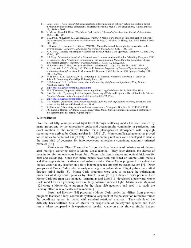
Monte Carlo programs are based on a technique proposed first by Metropolis and Ulam [18]. The main idea is the use of a stochastic approach to model a physical phenomenon. In the biomedical field, Monte Carlo programs have been used to model laser tissue interactions, fluorescence and many other phenomena [19,20]. In Standard Monte Carlo the user is interested only in the distribution of absorbed, transmitter or reflected photons; in the polarized Monte Carlo other parameters must be tracked. A flow-chart that includes both Standard and Polarized Monte Carlo main steps is shown in Figure 1. The gray boxes are necessary only in the Polarized Monte Carlo; all other steps must be included in both approaches.
A substantial difference between the polarized and standard Monte Carlo is the choice of the azimuthal and scattering angles. In the standard Monte Carlo the scattering angle α is chosen from a phase function, the most commonly used one is the Henyey-Greenstein phase function. Generally an azimuthal angle ψ is chosen uniformly between 0 and 2π . In the polarized Monte Carlo the scattering angle and the azimuth angle are chosen by a “rejection method” (STEP C) that will be discussed in section 9.
4
Fig. 1. - Flow chart of Polarized Monte Carlo program, the white cells are used in Standard Monte Carlo programs the gray cells are specific of Polarized Light Monte Carlo programs
An important feature of all polarization codes is tracking the reference plane used to describe the polarization of the photon. Since the status of polarization of a field is defined with respect to the reference plane, the reference plane must be defined (STEP A) and updated for each scattering event (STEP D). The different ways of tracking the reference plane account for the three different Monte Carlo programs described and are presented in detail in the next sections.
3. Method 1- Meridian Planes Monte Carlo
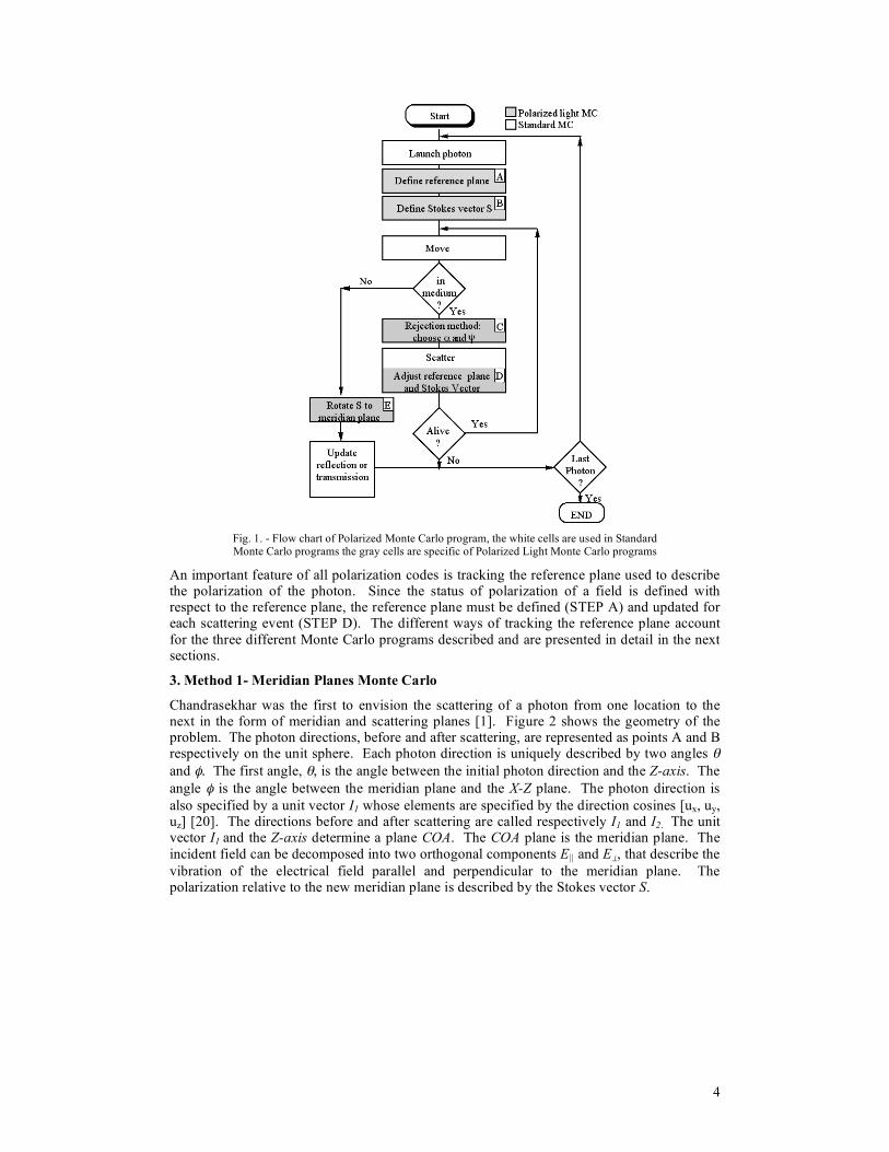
Chandrasekhar was the first to envision the scattering of a photon from one location to the next in the form of meridian and scattering planes [1]. Figure 2 shows the geometry of the problem. The photon directions, before and after scattering, are represented as points A and B respectively on the unit sphere. Each photon direction is uniquely described by two angles θ and φ. The first angle, θ, is the angle between the initial photon direction and the Z-axis. The angle φ is the angle between the meridian plane and the X-Z plane. The photon direction is also specified by a unit vector I1 whose elements are specified by the direction cosines [ux, uy, uz] [20]. The directions before and after scattering are called respectively I1 and I2. The unit vector I1 and the Z-axis determine a plane COA. The COA plane is the meridian plane. The incident field can be decomposed into two orthogonal components E|| and E⊥, that describe the vibration of the electrical field parallel and perpendicular to the meridian plane. The polarization relative to the new meridian plane is described by the Stokes vector S.
5
Fig. 2 - Meridian planes geometry. The photon’s direction of propagation before and after scattering is I1
, and I2 respectively. The plane COA defines the meridian plane before and after scattering.
When a scattering event occurs a new meridian plane is created by the new direction of propagation I2 and the Z-axis, the Stokes vector must be transformed so that the polarization is properly represented with respect to the new meridian plane. Two rotations of the Stokes vector, in and out of the scattering plane, are required by this method.
4. Method 2 –Euler Monte Carlo
The second method was developed by Bartel and Hielsher [14] and is based on the following idea: the photon polarization reference frame is tracked via a triplet of unit vectors that are rotated by an azimuth and scattering angle at each scattering step. The unit vectors are rotated using Euler angles by general transformation matrices [22]. In our implementation only two vectors are rotated for every scattering event v and u; the third unit vector is implicitly defined by the cross product of v and u and is calculated only when a photon reaches a boundary. The advantages of this method is that the Stokes vector is rotated only once for each scattering event instead of twice as in the meridian plane method. An added advantage is that the propagation of the unit vectors is straightforward and was easier to implement.
5. Method 3 –Quaternion Monte Carlo
The last method is based on quaternion algebra. Benoit and Clary [23] used a quaternion formulation to perform calculations on molecular clusters using quantum diffusion Monte Carlo. Richartz and Hsu [24] used quaternions to calculate the rotations and retardations of a polarized beam going through optical devices. We used quaternion algebra to track the polarization reference plane. Quaternions offer an elegant and intuitive way of handling rigid body rotations [22]. A quaternion is a 4-tuple of real numbers; it is an element of R4.
( )1 2 3, , ,oq q q q=q (1)
A quaternion can also be defined as the sum of a scalar part q0 and a vector part Γ in R3 of the form:
0 0 1 2 3q q q q q= + = + + +q i j k! (2)
6
Quaternions can be used as rotational operators. The vector part Γ is the rotational axis and the scalar part q0 is the angle of rotation. Multiplying a vector t by the quaternion q is equivalent to rotating the vector t around the vector Γ by the angle q0. To multiply a quaternion q by a vector t the latter must be converted into quaternion form. The vector t becomes a quaternion T whose scalar part is equal to 0 and whose vector part is equal to t:
1 2 30 0 t t t= + = + + +t i j k!
The quaternion product is defined as:
0
20 ( ) 2 ( ) 2 oq q= + ! " + " + #q t t t$ $ $ $ $ $ (3)
6. Polarized light Monte Carlo
We explain a Monte Carlo program in detail following the steps of the flowchart in figure 1. The steps for all three different methods will be described in parallel.
7. Launch
The first step in every Monte Carlo program is to launch one of several million photons in a media. Depending on the geometry of the beam (Gaussian or pencil beam are typical beam shapes) and the incident angle, different launching positions and photon directions cosines must be considered. When the polarization of the field is included some additional steps must be taken. The reference frame of the field must be defined and the Stokes vector describing the incident field polarization must be declared. For illumination perpendicular to the X-Y plane, the initial photon direction is defined by the following direction cosines [ux, uy, uz] = [0, 0, 1].
7.1 Launch - Meridian Planes Monte Carlo
The polarization of the photon is relative to the meridian plane.
Fig 1, STEP A: The meridian plane begins with φ=0, and the reference frame is initially equal to the x-z plane. The initial Stokes vector is relative to this meridian plane.
Fig 1, STEP B: The status of polarization of the launched photon S = [I Q U V] specified relative to the X-Z plane. For example, if the user selects a Stokes vector S=[1 1 0 0] the launched photon will be linearly polarized parallel to the X-Z plane.
7.2 Launch- Euler Monte Carlo and Quaternion Monte Carlo
For both the Euler Monte Carlo and the Quaternion Monte Carlo we may select the initial reference frame.
Fig 1, STEP A: We use two unit vectors v and u to define the E field reference frame.
[ ]
[ ]
, , 0, 1, 0
, , 0, 0, 1
x y z
x y z
v v v
u u u
! "= =# $
! "= =# $
v
u
Where the unit vector u represents the direction of photon propagation. Fig 1, STEP B: For any considered status of polarization of the incident field we define a Stokes vector S = [I Q U V] whose reference frame was established in step B; for example: if we want to model an incident field perpendicular to the reference plane we have to assume a Stokes vector S = [1 -1 0 0].
7
8 Move
The move step in polarized light Monte Carlo programs is executed as in a standard Monte Carlo program. The photon is moved a propagation distance Δs that is calculated based on pseudo random number
!
" generated in the interval (0,1].
!
"s = #ln($ )
µt
(4)
where µt = µa + µs, µa is the absorption coefficient, and µs is the scattering coefficient of the media. The mean free path between every scattering and absorption event is 1/µt. The trajectory of the photon is characterized by the direction cosines [ux, uy, uz]. Following Witt [21] the photon position is updated to a new position [x', y', z'] with the following equations:
'
'
'
x
y
z
x x u s
y y u s
z z u s
= + !
= + !
= + !
(5)
9 Drop
As in standard Monte Carlo code the absorption of light by a dye or an absorbing material present in the scattering media is tracked by giving a weight W to a photon and updating this weight after every absorption step according to the media albedo.
!
albedo =µs
µs+ µ
a
(6)
The albedo is the fractional probability of being scattered, 1-albedo is the fractional probability of being absorbed. The weight of the photon is initially equal to 1. The photon propagates through an absorbing media; after n steps the weight of the photon is equal to (albedo)n. In our Monte Carlo programs we use matched boundaries so we do not consider weight reduction due to the Fresnel interfaces as in standard Monte Carlo. When the weight of the photon reaches a threshold level the photon is terminated and is considered completely absorbed. If the photon exits the media with a certain weight W the corresponding Stokes vector is multiplied by W to keep in to account the photon attenuation.
out
I I W
Q Q W
U U W
V V W
!" # " #$ % $ %!$ % $ %=$ % $ %!$ % $ %
!& ' & '
(7)
10. Rejection Method
A fundamental problem in every Monte Carlo program with polarization information is the choice of the angles α (angle of scattering) and β (angle of rotation into the scattering plane), Figure 2. These angles are selected based on the phase function of the considered scatterers and a rejection method. A detailed description of how to implement a rejection method can be found in [16]. The phase function P(α,β) of spheres for incident light with a Stokes vector So= [Io, Qo, Uo, Vo] is
!
P ",#( ) = s11 "( )Io + s12 "( ) Qo cos 2#( ) +Uo sin 2#( )[ ] (8)
The parameters s11(α) and s12(α) are two elements of the scattering matrix M(α)
8
( ) ( )( ) ( )
( ) ( )( ) ( )
11 12
12 11
33 34
34 33
0 0
0 0( )
0 0
0 0
s s
s sM
s s
s s
! !
! !!
! !
! !
" #$ %$ %=$ %$ %
&$ %' (
(9)
The scattering matrix M(α) determines the polarization properties of the scattering element; we considered spheres. The matrix M(α) is symmetrical in the spherical case. The terms s11(α), s12(α), s34(α), and s33(α) are related to the scattered amplitudes S1 and S2 [27].
( )
( )
( )
( )
2 2
11 2 1
2 2
12 2 1
* *
33 2 1 2 1
* *
34 1 2 2 1
1
2
1
2
1
2
2
s S S
s S S
s S S S S
is S S S S
= +
= !
= +
= ! !
(10)
Where we omitted the angular α dependence. S1 and S2 depend from the size parameter x, the complex index of refraction of the particle nparticle, the Riccati-Bessel functions, the spherical Bessel functions, and the spherical Henkel functions; a more in depth explanation of these parameters can be found in reference [29]. In our Monte Carlo programs S1 and S2 for every scattering angle are obtained from a Mie scattering program [ 27,28].
The phase function P(α,β) has a bivariate dependence on angles α and β. For unpolarized light where So=[1, 0, 0, 0], the phase function becomes a function of just the single variable α,
!
P "( ) = s11"( ) (11)
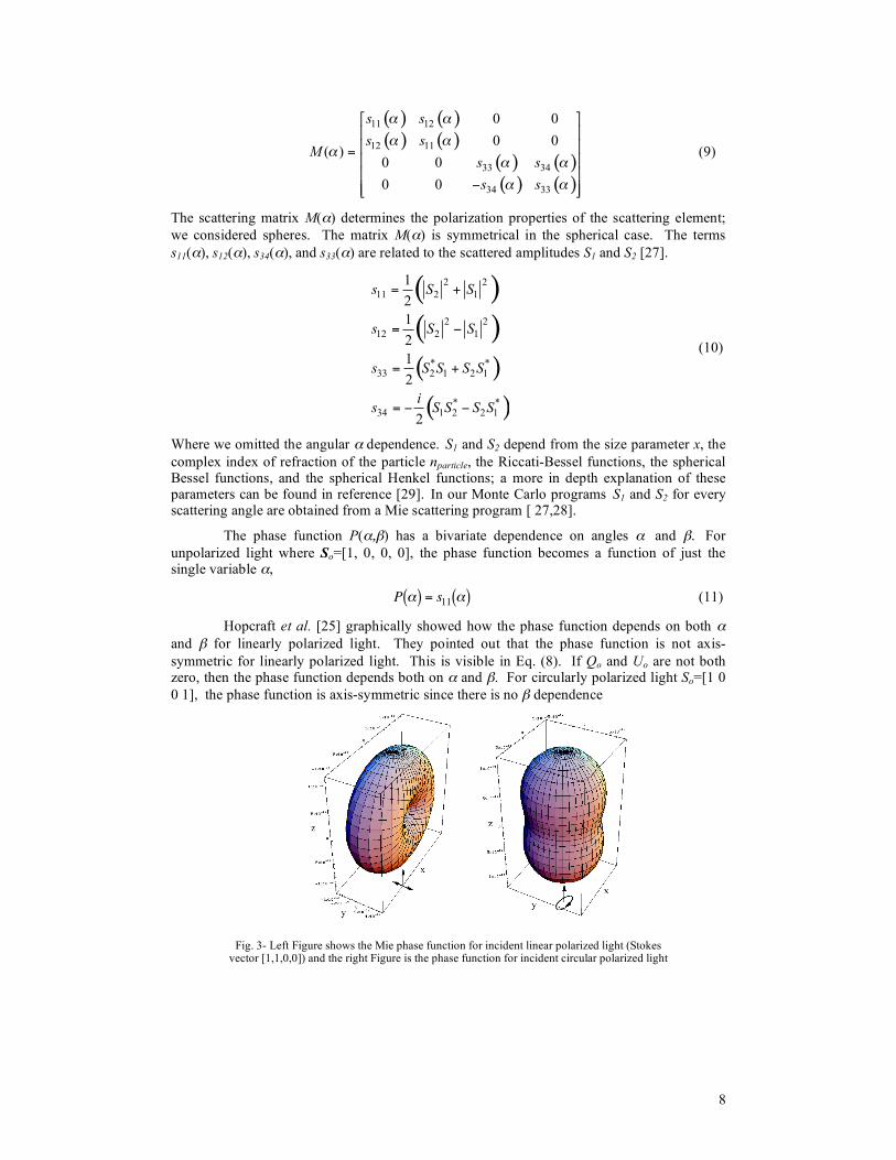
Hopcraft et al. [25] graphically showed how the phase function depends on both α and β for linearly polarized light. They pointed out that the phase function is not axis-symmetric for linearly polarized light. This is visible in Eq. (8). If Qo and Uo are not both zero, then the phase function depends both on α and β. For circularly polarized light So=[1 0 0 1], the phase function is axis-symmetric since there is no β dependence
Fig. 3- Left Figure shows the Mie phase function for incident linear polarized light (Stokes vector [1,1,0,0]) and the right Figure is the phase function for incident circular polarized light

9
(Stokes vector [1,0,0,1]). The sphere diameter is 10 nm in air, the incident wavelength is 543 nm, the index of refraction of the sphere is 1.59.
Our simulations of phase function intensities for linear and circular incidence agree with the simulations done by Hopcraft et al. and can be seen in Figure 3.
These simulations show the Mie phase function for linear polarized incidence and circular polarized incidence. The asymmetry of the phase function along the Z-axis for linear incidence is evident. In this figure, the phase function shows a strong dip at 90˚. A small sphere size (diameter = 10 nm) was used in both graphs with index of refraction 1.59.
Fig1, STEP C: The rejection method [26] may be used to generate random variables with a particular distribution. For functions of a single variable, two random numbers are generated. First, Prand is a uniform random deviate between 0 and 1. Second αrand is generated uniformly between 0 and π. The angle αrand is accepted as the new scattering angle if Prand ≤ P(αrand). If Prand>P(αrand) αrand and Prand are re-generated and the test is repeated.
When an angle αrand is accepted a similar process is implemented to calculate a new angle βrand. For a bivariate distribution like Eq. (7), three random numbers are generated αrand, Prand, and βrand. The angle β is uniformly distributed between 0 and 2π. If Prand ≤ P(αrand, βrand) then both αrand, ψrand are accepted as the new angles.
11 Scatter
Fig1 STEP D. The scattering step is significantly different in each of the three programs, but it always includes at least one rotation of the Stokes vector reference plane and one multiplication for the scattering matrix M(α).
11.1 Scatter - Meridian Planes Monte Carlo
Three operations are necessary to scatter a photon and track its polarization; these operations are graphically described in the Figures 4, 5, 6, and 7. The E field is originally defined with respect to a meridian plane COA. The field (visible in all Figures as blue lines) can be decomposed into its parallel and perpendicular components E|| and E⊥.
Fig. 4 -Visual description of the rotations necessary to transfer the reference frame from one meridian plane to the next. Initially the electrical field E is defined with respect to the meridian
plane COA.
Once the scattering angle α and azimuth angle β have been generated with the rejection method (section 9) the Stokes vector is manipulated three times, the three manipulation will be described in the next three paragraphs.
10
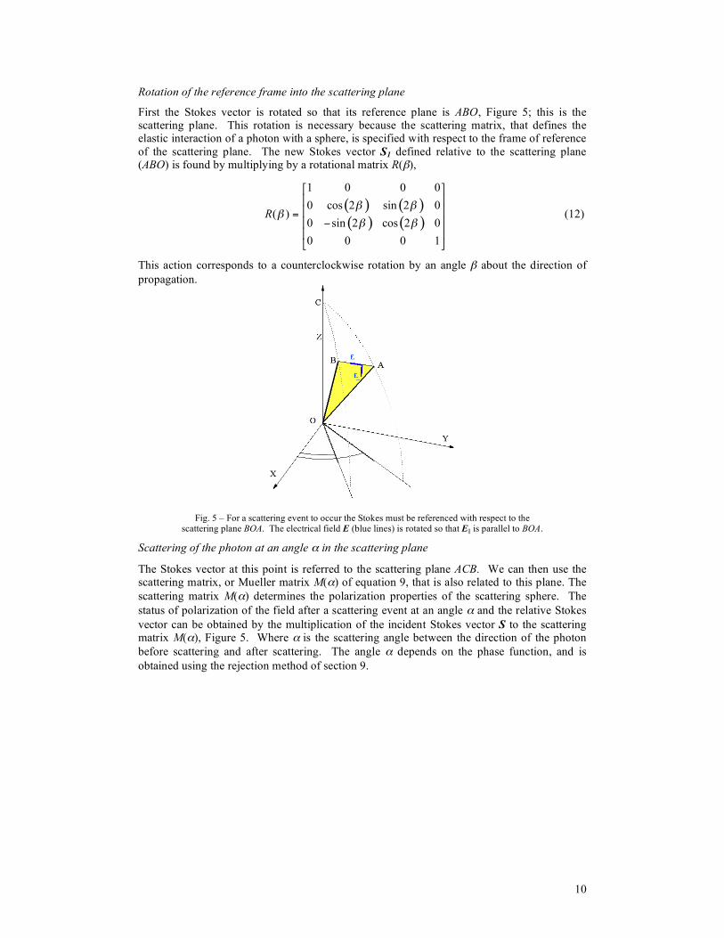
Rotation of the reference frame into the scattering plane
First the Stokes vector is rotated so that its reference plane is ABO, Figure 5; this is the scattering plane. This rotation is necessary because the scattering matrix, that defines the elastic interaction of a photon with a sphere, is specified with respect to the frame of reference of the scattering plane. The new Stokes vector S1 defined relative to the scattering plane (ABO) is found by multiplying by a rotational matrix R(β),
( ) ( )( ) ( )
1 0 0 0
0 cos 2 sin 2 0( )
0 sin 2 cos 2 0
0 0 0 1
R! !
!! !
" #$ %$ %=$ %&$ %' (
(12)
This action corresponds to a counterclockwise rotation by an angle β about the direction of propagation.
Fig. 5 – For a scattering event to occur the Stokes must be referenced with respect to the scattering plane BOA. The electrical field E (blue lines) is rotated so that E|| is parallel to BOA.
Scattering of the photon at an angle α in the scattering plane
The Stokes vector at this point is referred to the scattering plane ACB. We can then use the scattering matrix, or Mueller matrix M(α) of equation 9, that is also related to this plane. The scattering matrix M(α) determines the polarization properties of the scattering sphere. The status of polarization of the field after a scattering event at an angle α and the relative Stokes vector can be obtained by the multiplication of the incident Stokes vector S to the scattering matrix M(α), Figure 5. Where α is the scattering angle between the direction of the photon before scattering and after scattering. The angle α depends on the phase function, and is obtained using the rejection method of section 9.

11
Fig. 6– After a scattering event the Stokes vector is defined respect to the plane BOA.
The direction cosines are updated to take into account the new direction. The new direction cosines will be called û. The new trajectory [ûx, ûy, ûz] is calculated based on the angle α and β and on the current trajectory [ux, uy, uz].
If |uz| ≈ 1:
!
ˆ u x = sin "( ) cos #( )ˆ u y = sin "( ) sin 2#( )
ˆ u z = cos "( )uz
uz
(13)
for all other cases:
( ) ( ) ( ) ( )
( ) ( ) ( ) ( )
( ) ( ) ( ) ( ) ( )
2
2
2
1ˆ sin cos sin cos
1
1ˆ sin cos sin cos
1
ˆ 1 sin cos cos sin cos
z
z
z
x x y y x
y x z x y
z y z x z
u u u u u
u
u u u u u
u
u u u u u u
! " " !
! " " !
! " " " !
# $= % +& '%
# $= % +& '%
# $= % % +& '
(14)
Return the reference frame to a new meridian plane
The Stokes vector is multiplied by the rotational matrix R(-γ) so that it is referenced to the meridian plane COB (Figure 7). The angle γ was calculated by Hovenier [30],
( )( )2 2
ˆ coscos
ˆ1 cos 1
z z
z
u u
u
!"
!
# +=
± # #
(15)
where α is the scattering angle and the plus sign is taken when π <β <2π and the minus sign is taken when 0 <β <π. In summary the Stokes vector Snew after scattering is obtained from the Stokes vectors before the scattering event S using the following matrix multiplication:
( ) ( ) ( )new! " #= $S R M R S (16)
12
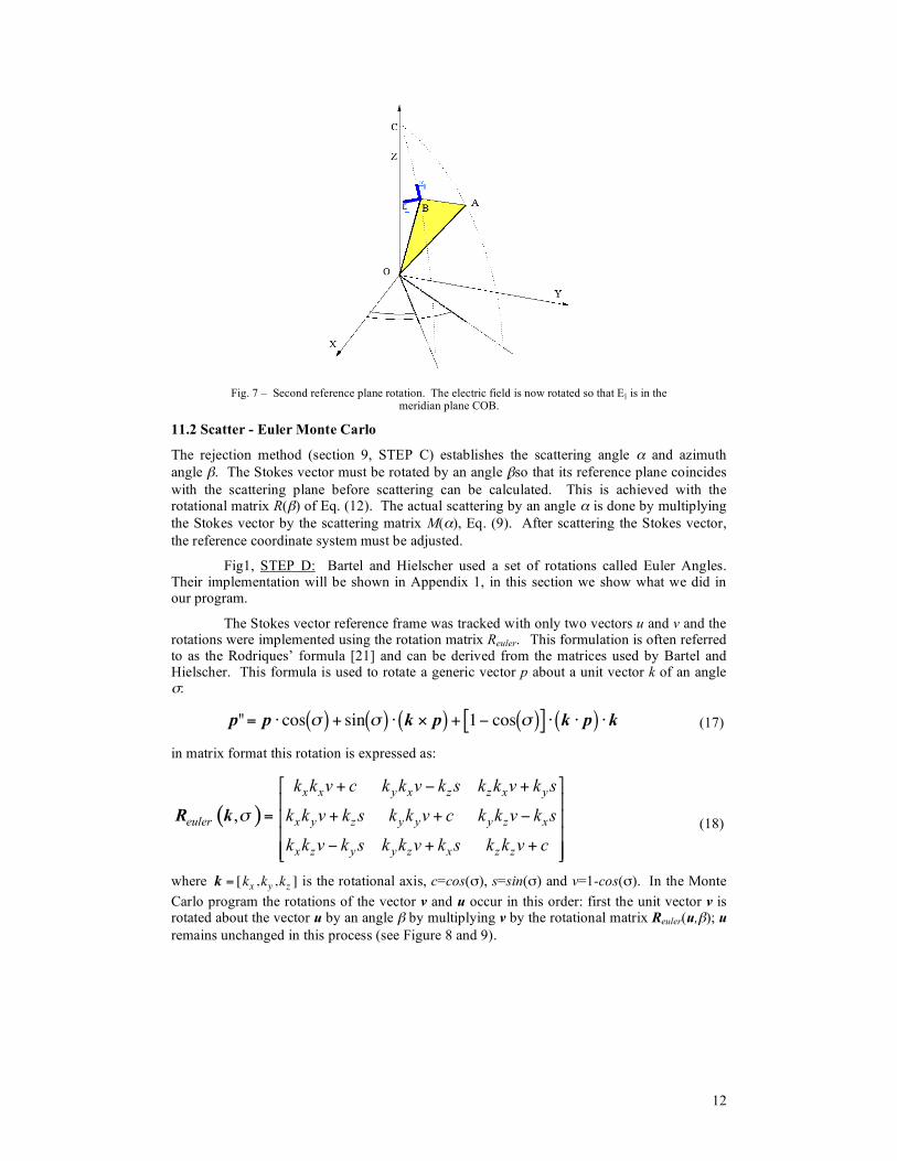
Fig. 7 – Second reference plane rotation. The electric field is now rotated so that E|| is in the meridian plane COB.
11.2 Scatter - Euler Monte Carlo
The rejection method (section 9, STEP C) establishes the scattering angle α and azimuth angle β. The Stokes vector must be rotated by an angle β so that its reference plane coincides with the scattering plane before scattering can be calculated. This is achieved with the rotational matrix R(β) of Eq. (12). The actual scattering by an angle α is done by multiplying the Stokes vector by the scattering matrix M(α), Eq. (9). After scattering the Stokes vector, the reference coordinate system must be adjusted.
Fig1, STEP D: Bartel and Hielscher used a set of rotations called Euler Angles. Their implementation will be shown in Appendix 1, in this section we show what we did in our program.
The Stokes vector reference frame was tracked with only two vectors u and v and the rotations were implemented using the rotation matrix Reuler. This formulation is often referred to as the Rodriques’ formula [21] and can be derived from the matrices used by Bartel and Hielscher. This formula is used to rotate a generic vector p about a unit vector k of an angle σ:
!
p"= p " cos #( ) + sin #( ) " k $ p( ) + 1% cos #( )[ ] " k " p( ) "k (17)
in matrix format this rotation is expressed as:
( ),x x y x z z x y
euler x y z y y y z x
x z y y z x z z
k k v c k k v k s k k v k s
k k v k s k k v c k k v k s
k k v k s k k v k s k k v c
!
" #+ $ +% &
= + + $% &% &
$ + +% &' (
R k (18)
where
!
k = [kx ,ky ,kz ] is the rotational axis, c=cos(σ), s=sin(σ) and v=1-cos(σ). In the Monte Carlo program the rotations of the vector v and u occur in this order: first the unit vector v is rotated about the vector u by an angle β by multiplying v by the rotational matrix Reuler(u,β); u remains unchanged in this process (see Figure 8 and 9).
13
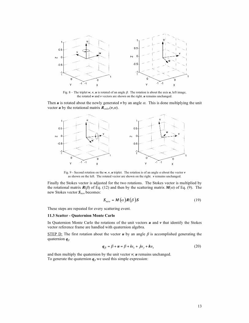
Fig. 8 – The triplet w, v, u is rotated of an angle β. The rotation is about the axis u, left image,
the rotated w and v vectors are shown on the right. u remains unchanged.
Then u is rotated about the newly generated v by an angle α. This is done multiplying the unit vector u by the rotational matrix Reuler(v,α).
Fig. 9 - Second rotation on the w, v, u triplet. The rotation is of an angle α about the vector v as shown on the left. The rotated vector are shown on the right. v remains unchanged.
Finally the Stokes vector is adjusted for the two rotations. The Stokes vector is multiplied by the rotational matrix R(β) of Eq. (12) and then by the scattering matrix M(α) of Eq. (9). The new Stokes vector Snew becomes:
( ) ( )new! "=S M R S (19)
These steps are repeated for every scattering event.
11.3 Scatter - Quaternion Monte Carlo
In Quaternion Monte Carlo the rotations of the unit vectors u and v that identify the Stokes vector reference frame are handled with quaternion algebra.
STEP D: The first rotation about the vector u by an angle β is accomplished generating the quaternion qβ
!
q" = " + u = " + iux + juy + kuz (20)
and then multiply the quaternion by the unit vector v; u remains unchanged. To generate the quaternion qβ we used this simple expression:

14
!
q"1 = ux sin"
2
#
$ %
&
' (
q" 2 = uy sin"
2
#
$ %
&
' (
q" 3 = uz sin"
2
#
$ %
&
' (
q" 4 = cos"
2
#
$ %
&
' (
(21)
The multiplication of the quaternion qβ by a vector v is obtained as in Eq. (20).
The second rotation is by an angle α about the axis v. This is done generating the quaternion qα
!
q" =" + v =" + ivx + jvy + kvz (22)
and multiplying it by the unit vector u. These steps are frequently optimized for speed and computational efficiency [32]; in our program we use the simplest and more intuitive implementation and not necessarily the fastest one. The Stokes vector is also adjusted for the two rotation as in Eq. (19).
11 Photon life and boundaries
The life of a photon ends when the photon passes through a boundary or when its weight W value falls below a threshold (typically 0.001) as in standard Monte Carlo.
11.1 Meridian Planes Monte Carlo
When the photon reaches one of the boundaries and is ready to be collected by a detector, one last rotation of the Stokes vector is necessary to put the photon polarization in the reference frame of the detector.
STEP E: For a photon backscattered from a slab, the last rotation to the meridian plane of the detector is by an angle ϕ
!
" = tan#1 uy
ux
$
% &
'
( ) (23)
The Stokes vector of the reflected photon is multiplied one final time by R(ϕ). For a transmitted photon the angle ϕ is:
!
" = # tan#1uy
ux
$
% &
'
( ) (24)
Since Stokes vectors can be superimposed, all photons reaching a boundary can be added once they have been rotated to the reference frame of the detector.
11.2 Euler and Quaternion Monte Carlo
When the photon has reached one of the boundaries and is ready to be collected by a detector two final rotations of the Stokes vector are necessary to put the photon status of polarization in the detector reference frame.
STEP E: The first rotation is needed to return the Stokes vector to the meridian plane. To do this w is reconstructed as the cross product of v and u.
= !w v u (26)
15
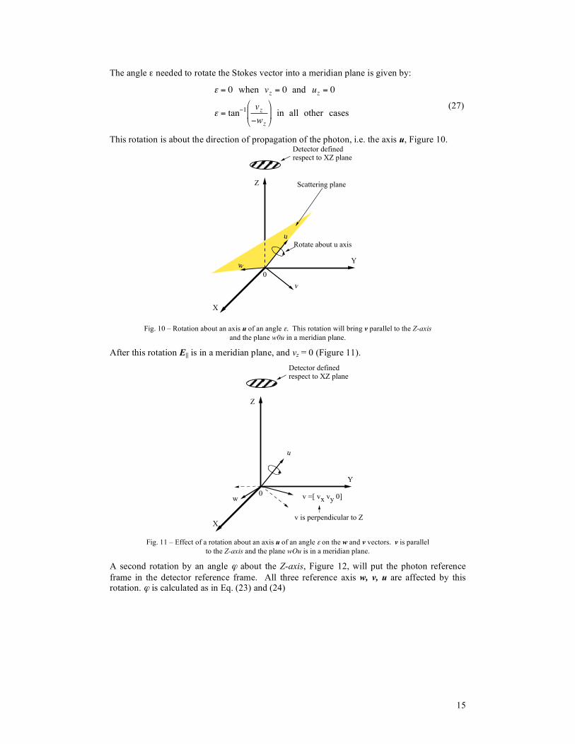
The angle ε needed to rotate the Stokes vector into a meridian plane is given by:
!
" = 0 when vz = 0 and uz = 0
" = tan#1 vz
#wz
$
% &
'
( ) in all other cases
(27)
This rotation is about the direction of propagation of the photon, i.e. the axis u, Figure 10.
X
Y
Z
w
0
Scattering plane
Rotate about u axis
Detector definedrespect to XZ plane
v
u
Fig. 10 – Rotation about an axis u of an angle ε. This rotation will bring v parallel to the Z-axis and the plane w0u in a meridian plane.
After this rotation E|| is in a meridian plane, and vz = 0 (Figure 11).
X
Y
Z
0
v is perpendicular to Z
Detector definedrespect to XZ plane
w v =[ vx vy 0]
u
Fig. 11 – Effect of a rotation about an axis u of an angle ε on the w and v vectors. v is parallel
to the Z-axis and the plane wOu is in a meridian plane.
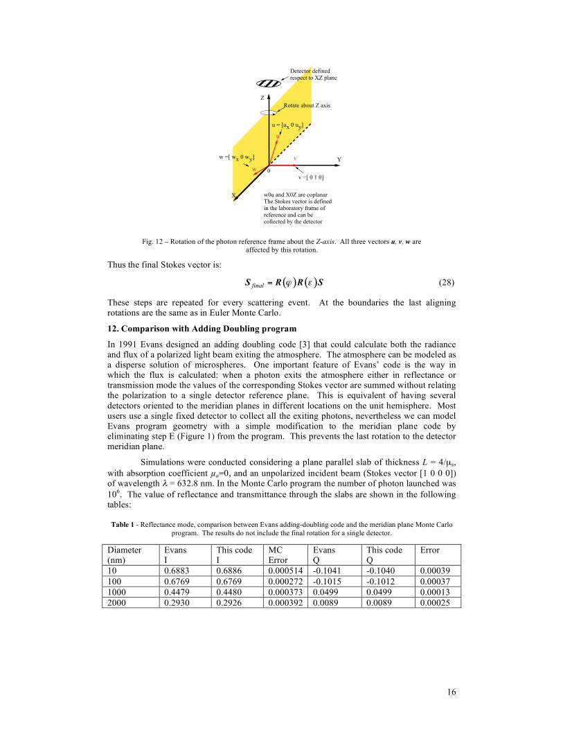
A second rotation by an angle ϕ about the Z-axis, Figure 12, will put the photon reference frame in the detector reference frame. All three reference axis w, v, u are affected by this rotation. ϕ is calculated as in Eq. (23) and (24)
16
X
Y
Z
0v =[ 0 1 0]
Rotate about Z axis
Detector definedrespect to XZ plane
v
u
w
w =[ wx 0 wy]
u = [ux 0 uy]
w0u and X0Z are coplanarThe Stokes vector is defined in the laboratory frame of reference and can be collected by the detector
Fig. 12 – Rotation of the photon reference frame about the Z-axis. All three vectors u, v, w are
affected by this rotation.
Thus the final Stokes vector is:
( ) ( )final ! "=S R R S (28)
These steps are repeated for every scattering event. At the boundaries the last aligning rotations are the same as in Euler Monte Carlo.
12. Comparison with Adding Doubling program
In 1991 Evans designed an adding doubling code [3] that could calculate both the radiance and flux of a polarized light beam exiting the atmosphere. The atmosphere can be modeled as a disperse solution of microspheres. One important feature of Evans’ code is the way in which the flux is calculated: when a photon exits the atmosphere either in reflectance or transmission mode the values of the corresponding Stokes vector are summed without relating the polarization to a single detector reference plane. This is equivalent of having several detectors oriented to the meridian planes in different locations on the unit hemisphere. Most users use a single fixed detector to collect all the exiting photons, nevertheless we can model Evans program geometry with a simple modification to the meridian plane code by eliminating step E (Figure 1) from the program. This prevents the last rotation to the detector meridian plane.
Simulations were conducted considering a plane parallel slab of thickness L = 4/µs, with absorption coefficient µa=0, and an unpolarized incident beam (Stokes vector [1 0 0 0]) of wavelength λ = 632.8 nm. In the Monte Carlo program the number of photon launched was 106. The value of reflectance and transmittance through the slabs are shown in the following tables:
Table 1 - Reflectance mode, comparison between Evans adding-doubling code and the meridian plane Monte Carlo program. The results do not include the final rotation for a single detector.
Diameter (nm)
Evans I
This code I
MC Error
Evans Q
This code Q
Error
10 0.6883 0.6886 0.000514 -0.1041 -0.1040 0.00039 100 0.6769 0.6769 0.000272 -0.1015 -0.1012 0.00037 1000 0.4479 0.4480 0.000373 0.0499 0.0499 0.00013 2000 0.2930 0.2926 0.000392 0.0089 0.0089 0.00025

17
Table 2 - Transmission mode, comparison between Evans adding doubling code and the meridian plane Monte Carlo program. The results are not corrected for a single detector.
Diameter (nm)
Evans I
This code I
MC Error
Evans Q
This code Q
MC Error
10 0.31167 0.3111 0.0005 -0.012281 -0.0121 0.0005 100 0.32301 0.3231 0.0003 -0.012844 -0.0126 0.0002 1000 0.55201 0.5520 0.0003 0.02340 0.0234 0.0005 2000 0.70698 0.7067 0.0004 0.01197 0.0119 0.0002
The error for the Monte Carlo runs was the standard deviation of five different runs where only the seed of the random generator was changed. The difference in between our code and Evans results is always less than 1%.
13. Conclusions
In this paper three different Monte Carlo programs that keep track of the status of polarization after every scattering event were described. The three programs are significantly different from each other yet they yield the same numerical results.
The programs were developed for Unix platform in C programming language. All three programs run at approximately the same speed. The three codes are available for download at [31].
The Euler’s angle Monte Carlo is easy to implement and intuitive, with a triplet of unit vectors following the photon reference frame after every scattering event. Euler’s rotational matrices are well known since they are often used in rigid body rotations. Moreover since for any scattering event only one rotation of the reference frame is necessary the program should in principle be faster that the meridian plane method.
The quaternion Monte Carlo is an elegant solution. Quaternion rotations are used more and more often in computer science to handle animations. Many improvements are available to simplify the generation of the quaternion plus the multiplicative step in order to make them faster [32,33]. Moreover Richartz and Hsu [24] demonstrated that quaternions can be used to simulate a material retardation, hence this methodology could be particularly useful in the modeling of polarized transfer in biological media, where birefringence and retardation play a large role. We intend to explore these algorithms in the future.
The compilation of these three models was lengthy, seemingly correct solutions were proven wrong by further testing. A key issue we identified during this process relates to the exiting routine and the backscattered reflection of photons. Many of the papers dealing with polarized Monte Carlo program use as proof of the goodness of their code the shapes of the backscattered Mueller matrix from a solution of microsphere. Since many of the elements of the Mueller matrix are axially symmetric an erroneous exiting routine could still generate apparently correct answers. The best way to test for this is to launch photons at a small angle to the normal (~30 degrees). This assures the breaking of symmetry, the backscattered pattern will be better suited for experimental comparison.
Another issue we encountered in the compilations of our Monte Carlo programs was related to the subdivision of the scattering function. Generally a subdivision of 180 angles is acceptable, in Henyey Greenstein based Monte Carlo programs. In our Mie theory based programs the subdivision of the scattering function had to be larger than 1000 angles to obtain accurate values of total reflectance and total transmittance.
In previous papers [14, 16] have discussed the correct implementation of the rejection function that chooses the scattering angle α and azimuth angle β. Some author such as Bartel and Hiescher, select first the azimuth angle uniformly between 0 and π and then enter the rejection method algorithm where the scattering angle is selected based on the
18
original choice of β. Rakovic et al. [16] showed that the correct choice of α and β is obtained selecting both angles in the loop of the rejection method. We implemented both method and realized that although Rakovic et al. are theoretically the two numerical implementation are numerically very similar. Moreover the rejection method is a bottleneck for the Monte Carlo program, optimizing this section of the program would improve dramatically their efficiency.
Significant experimental testing was performed on all three programs. The results of these tests will be shown in the next paper [34].
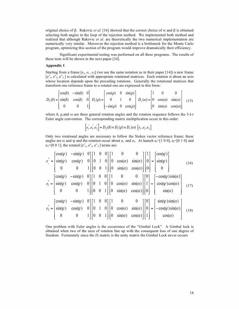
Appendix 1
Starting from a frame [er, el , e3] (we use the same notation as in their paper [14]) a new frame
[e″r, e″l, e″3 ] is calculated with appropriate rotational matrices. Each rotation is about an axis
whose location depends upon the preceding rotations. Generally the rotational matrices that transform one reference frame to a rotated one are expressed in this form:
!
D3 (") =
cos(") #sin(") 0
sin(") cos(") 0
0 0 1
$
%
& & &
'
(
) ) )
Dl(*) =
cos(*) 0 sin(*)
0 1 0
#sin(*) 0 cos(*)
$
%
& & &
'
(
) ) )
Dr(+) =
1 0 0
0 cos(+) sin(+)
0 sin(+) cos(+)
$
%
& & &
'
(
) ) )
(15)
where δ, ρ,and ω are three general rotation angles and the rotation sequence follows the 3-l-r Euler angle convention. The corresponding matrix multiplication occur in this order:
!
er
",el
",e3
"[ ] = D3 (") #Dl($) #D
r(%) e
r,el,e3[ ]
Only two rotational angles are necessary to follow the Stokes vector reference frame; these angles are α and ψ and the rotation occur about er and e3. At launch er=[1 0 0], el=[0 1 0] and e3=[0 0 1], the rotated [e″r, e″l, e″3
] terms are:
"
cos( ) sin( ) 0 1 0 0 1 0 0 1 cos( )
sin( ) cos( ) 0 0 1 0 0 cos( ) sin( ) 0 sin( )
0 0 1 0 0 1 0 sin( ) cos( ) 0 0r
e
! ! !
! ! " " !
" "
#$ % $ % $ % $ % $ %& ' & ' & ' & ' & '
= =& ' & ' & ' & ' & '& ' & ' & ' & ' & '( ) ( ) ( ) ( ) ( )
(16)
"
cos( ) sin( ) 0 1 0 0 1 0 0 0 cos( )sin( )
sin( ) cos( ) 0 0 1 0 0 cos( ) sin( ) 1 cos( ) cos( )
0 0 1 0 0 1 0 sin( ) cos( ) 0 sin( )
le
! ! ! "
! ! " " ! "
" " "
# #$ % $ % $ % $ % $ %& ' & ' & ' & ' & '
= =& ' & ' & ' & ' & '& ' & ' & ' & ' & '( ) ( ) ( ) ( ) ( )
(17)
"3
cos( ) sin( ) 0 1 0 0 1 0 0 0 sin( )sin( )
sin( ) cos( ) 0 0 1 0 0 cos( ) sin( ) 0 cos( )sin( )
0 0 1 0 0 1 0 sin( ) cos( ) 1 cos( )
e
! ! ! "
! ! " " ! "
" " "
#$ % $ % $ % $ % $ %& ' & ' & ' & ' & '
= = #& ' & ' & ' & ' & '& ' & ' & ' & ' & '( ) ( ) ( ) ( ) ( )
(18)
One problem with Euler angles is the occurrence of the “Gimbal Lock”. A Gimbal lock is obtained when two of the axes of rotation line up with the consequent loss of one degree of freedom. Fortunately since the Dl matrix is the unity matrix the Gimbal Lock never occurs