Through the Looking Glass: A WARPed Viewof Real Exchange Rate History∗

Douglas L. Campbell† Ju Hyun Pyun‡University of California, Davis The Korea University

May, 2014

AbstractCommonly used trade-weighted real exchange rate indices are computed as indices-of-indices, and thus do not adequately account for growth in trade with developing coun-tries. Weighted Average Relative Price (WARP) indices solve this problem but do notcontrol for productivity differences, as developing countries are observed to have lowerprice levels via the Balassa-Samuelson effect. In this paper, we remedy these problems intwo ways. First we propose a Balassa-Samuelson productivity adjustment to WeightedAverage Relative Price indices (BS-WARP). Secondly, we introduce a Weighted AverageRelative Unit Labor Cost index (WARULC) for manufacturing and show that this mea-sure does a much better job predicting trade imbalances and declines in manufacturingemployment than the IMF’s Relative ULC measure created as an index-of-indices. Ourseries reveal that for many countries currently mired in liquidity traps, relative pricesreached historic highs heading into the financial crisis of 2008. We document that in2002 – during the surprisingly sudden collapse in US manufacturing – US relative priceshad not been that high relative to trading partners since the worst year of the GreatDepression.

JEL Classification: F31, F32, N70, C43Keywords: Real Exchange Rate Indices, Relative Unit Labor Cost Indices,

Balassa-Samuelson, Trading Partner Substitution Bias∗We are indebted to comments received from seminar participants at UC Davis, Colby College, the

New Economic School, Santa Clara, and at the All-UC Economic History conference at Berkeley. Wewould also like to thank Paul Bergin, Robert Feenstra, Chris Meissner, Kim Ruhl, and John Devereuxfor their suggestions. Special thanks to Barry Eichengreen and the Berkeley Economic History Lab forproviding access to data resources. We would also like to thank the hardworking public servants at theBLS, the BEA, and the OECD for responding to data inquiries.†Visiting scholar, Berkeley Economic History Lab. UC Davis department address: Department

of Economics, One Shields Avenue, Davis, CA 95616, USA. Tel.: 1-812-679-8861, e-mail: dlcamp-bell@ucdavis.edu, Homepage: dougcampbell.weebly.com.‡Tel.: 82-2-3460-1190, e-mail: juhnpyun@gmail.com.

1 Introduction

One of the most important prices in any open economy is the real rate of exchange.Trade-weighted real exchange rate indices thus provide a useful guide to both policy-makers and academic economists as rough measures of the competiveness of a currencyin international trade.1 In this paper, we examine the methodology used to create theseindices, arguing that real exchange rate history needs to be viewed through the appro-priate looking glass. And what one finds there in this distorted world is that manykey events in economic history—the Asian Financial Crisis, the swift decline of Amer-ican manufacturing, the Great Depression, and the “Lesser Depression”, as well as theongoing structural US trade deficit—are cast in new light.

The most commonly used real exchange rate indices are constructed by the FederalReserve, the IMF, and the OECD as indices-of-indices. The levels of these series thusare not internationally comparable and they suffer from what we call a “trading partnersubstitution bias” problem, as they do not adequately account for growth in trade withdeveloping countries.2 India and China are assigned the same base value in these priceindices as are Switzerland and Germany, even though the latter have much higher pricesfor all years, which becomes problematic when trade increases with India and Chinarelative to countries with higher price levels. In a seminal contribution, Fahle, Marquez,and Thomas (2008) rewrote the prior 20 years of US real exchange rate history byshowing that a simple Weighted Average Relative Price (WARP) index implies that thedollar appreciated substantially more from 1990 to 2006 compared to “divisia” basedindices-of-indices produced by the Federal Reserve Board and the IMF. Fahle et al.(2008) also find that a geometric WARP index does a much better job of explaining

1We began this project while doing research on the impact of exchange rate movements on variouseconomic variables. We soon discovered, as Fahle et al. (2008) did, that the real exchange rate indicescreated by the Fed, the IMF, and the OECD, which have appeared widely in academic research, are notsuitable for many tasks for which they are often employed. In addition, there are no appropriate indiceswhich are publicly available for easy downloading, even for the modern era, much less historically.Any economist or policymaker who wants to consult a real exchange rate index must choose betweenplotting a series likely to mislead (often unwittingly), or else engage in the time-consuming task ofcreating a series from scratch. Thus most central bank presidents and heads of state, even in severelydepressed economies such as Ireland, have never seen a real exchange rate index for their own countrythat accounts for compositional changes in trade for the simple reason that none exist. Thus, part ofthe value-added of this paper is that we provide these indices for many countries on our website forfree, easy downloading.

2This problem is analagous to the “outlet substitution bias” problem with the CPI, and is alsoidentical to the index numbers problem highlighted by Houseman et al. (2011) and Inklaar (2013) inthe calculation of manufacturing productivity. Diewert et al. (2014) provide a nice overview of thegeneral issue, which they call “sourcing substitution bias” for the context of changing intermediateinput sources.

1

trade balances from the period 1970-2006 than divisia-based alternatives.First, we extend WARP to the period 1950-2011 using version 8.0 of the Penn World

Tables, which includes changes in terms of trade, and show that compared to WARPconstructed using version 7.1 of the PWT,WARP v8.0 implies that US prices appreciatednearly 16% more over the period 1990-2002 relative to trading partners. This featurecan help explain the rise in the structural current account deficit and sudden collapse intradables sector employment over that period. By 2011, according to the new version ofWARP the price level in the US was 10% higher than the price level of trading partners.In addition, compared to v7.1, v8.0 of the PWT implies lower US prices relative totrading partners in all periods but is much more pronounced before the late 1990s. Itshows less of a dollar appreciation in the 1980s, and for the Bretton Woods era, WARPlines up more closely with the Federal Reserve Board’s Broad Trade Weighted RealExchange Rate Index, which we also extend back to 1950 using the Fed’s methodology.

One problem with usingWARP as a measure of competitiveness is that poor countriesshould theoretically have lower price levels according to the Balassa-Samuelson effect.Having a price level twice that of Japan in 1946 has very different implications forbilateral competitiveness than having a price level twice that of Japan in 1986. Astraightforward resolution to this problem is to make a Balassa-Samuelson adjustmentto WARP (BS-WARP). Increased trade with less-developed countries will only resultin a stronger dollar index if these countries are undervalued relative to their level ofdevelopment. The index is conceptually similar to the Balassa-Samuelson residuals usedby Rodrik (2008) and many others in the literature on exchange rates and growth,except that the index proposed in this paper is a trade-weighted average of the differencebetween the US residual and the residuals of US trading partners.

The level of the BS-WARP index indicates a substantially more competitive dollarrelative to WARP for all years from 1950 to 2011, with the dollar actually 3% under-valued by 2011. This finding was not anticipated and is counterintuitive given the largestructural trade deficit. However, after the dollar’s dramatic rise in the 1980s, it alsotook several years after the dollar depreciated before trade was balanced, giving rise toan academic literature on hysteresis. The US BS-WARP index had fallen below unity be-cause the US Balassa-Samuelson residual had fallen close to zero by 2011 and US trade isbiased toward countries which also have richly-valued currencies such as Canada, Japan,and the Euro Area. That the US Balassa-Samuelson residual itself indicates that theUS price level is not overvalued (given US productivity) may in part be a function ofrelatively low US value-added taxes and tariffs, is distinct from the relative unit labor

2

cost data, and could be revised in the next round of revisions of the Penn World Tables.3

In the US case, directional changes in BS-WARP are broadly similar to the directionalchanges in WARP (the differences are far more pronounced for countries growing orcontracting quickly, such as Ireland, Korea, and Poland). The similarity between WARPand BS-WARP for the US after 2002 was not easily anticipated – the Balassa-Samuelsonadjustment lowers the RER for countries growing quickly, such as China, so it couldhave been expected that after 2002, the BS-WARP index would show a more moderatedepreciation as trade with fast-growing China increased. Using PWT v7.1, the BS-WARP index does show a more moderate depreciation after 2002, and was still 20%overvalued as of 2010. However, PWT version 8.0 marked up the growth in Chineseprices after 2005 and thus marked down the growth rate of Chinese GDP per capita by21% over this period, partly moderating the impact.

Of course, it has long been recognized that real exchange rate indices need to beadjusted for productivity. This is why economists have generally preferred to use realexchange rate indices computed using unit labor costs in manufacturing rather thanthose based on other measures, such as consumer prices. Commonly used real exchangerate indices computed by the IMF and the OECD using relative unit labor costs are alsocomputed as indices-of-indices and thus suffer from trading partner substitution bias. Inaddition, they use fixed trade weights and do not include China. We propose a simplegeometric Weighted Average Relative Unit Labor Cost index (WARULC), computed astotal labor income in manufacturing converted to the local currency at exchange ratesand total manufacturing output converted to the local currency at manufacturing PPP.We compute manufacturing PPP using PWT v8.0 methodology described in Feenstraet al. (2013), applying the Geary-Khamis indexing method to the manufacturing basicheadings of all six publicly available International Comparison Program (ICP) bench-mark years, and interpolating using manufacturing value-added growth rates reportedby country specific sources in between. The index we create shows a much greater dollarappreciation over time than the IMF or OECD indices, and by 2001 stood 32% higherthan the IMF’s index relative to 1975. Our index appears to do a superior job predict-ing trade imbalances and periods when relatively more import-competing manufacturingsectors experience relative declines in employment.

As of 2009, while China employed about 9 times as many man-hours in manufacturingthan did the US to produce slightly more, Chinese hourly wages in dollars were just $1.74

3The next version will include the 2011 ICP, and will be available in the fall of 2013. Subsequentdrafts of this paper after that time will update to the most recent version of the PWT.

3

compared to $35.18 for the US.4 Thus we calculate that Chinese unit labor costs wereabout 37% of US unit labor costs in 2009. Although full Chinese data on employmentand hours worked was unavailable through 2011, Chinese hourly wages went from being5% of US wages to 7% of US wages in those two years alone, while production rose24% in China versus just 10% for the US. Thus, while the gap appears to be closing,the picture that emerges of competitiveness from relative unit labor costs in the US vs.China is different from what emerges with the Balassa-Samuelson adjustment.

To the extent possible, we extend all indices over both space and time. For the US, weextend both “divisia” and WARP indices for the US historically for the period 1820-2010.The Thomas et al. WARP series spans 1970-2006, while the Fed’s broad trade-weightedreal exchange rate index starts in 1973. The Fed’s series commences at an inopportunetime as it misses the large depreciation at the end of the Bretton Woods period. Weextend both series back to 1950 using the same sample of countries, trade-weightingscheme and indexing methodology as the Federal Reserve. We also extend these seriesback to 1922 on a consistent sample of 30 countries, and back to 1820 for a sample offive countries. Compared to divisia, WARP implies a lower US price level in the periodbefore WWII relative to the Bretton Woods period and exhibits a slightly sharper dollarappreciation during the Great Depression, with a difference from 1928-1932 of 3%.

We also provide indices which adjust for domestic competition to allow compara-bility across different eras or countries. Firms located in large economies which tradelittle, such as the US in the 1950s, mostly compete domestically, while firms located insmall open economies largely compete internationally. Hence, the latter group will bemuch more affected by international competition. Indexes adjusted for domestic com-petition better match the stylized fact that the late 1990s and 2000s real exchange rateappreciation was a much larger shock to trade than the short spike in the dollar in the1980s. Additionally, we propose an improvement to the Federal Reserve Board’s tradeweights, but find that this leaves all indices little-changed, resulting in an increaseddollar appreciation from 1992-2002 of an additional 1%.

Internationally, we produce WARP, BS-WARP, and WARULC indices for majorEuropean nations in and out of the Euro zone. We find that for Italy, Greece, the UK,and the Russian Federation, the WARP and BS-WARP indices reveal a much greater

4These estimates use OECD data on US manufacturing employment and hours, which are basedon household survey data for the US which are used for international comparability, and governmentdata for Chinese employment. The better-known manufacturing employment numbers in the US comefrom the establishment survey, which shows 2 million workers in manufacturing. Chinese manufacturingoutput from the World Bank was converted into dollars at manufacturing PPP estimates, but wouldnot be substantially different in 2009 converting at exchange rates. The hourly wage data comes fromthe BLS.

4

real appreciation since 1990 than do the IMF’s divisia-based series. For example, in2010 the BS-WARP series for Italy stood more than 20% higher than the IMF’s seriesrelative to 1990, and in 2007, the UK’s WARP index also stood 20% higher relative to1990 than the IMF’s RER index. Conversely, Germany’s BS-WARP index is similarto its IMF CPI-based real effective exchange rate. This revision of relative prices isnot merely an academic curiosity given the economic problems now facing Europe. Itaccentuates the difficulties the European Central Bank faces in divising one monetarypolicy for countries with very disparate trends in relative prices measured relative totrading partners.

The Balassa-Samuelson adjusted index also reveals a substantial appreciation forthe relative price level of Greece, demonstrating that currency appreciation since 1990cannot merely be explained by Greece’s convergence in GDP as is often thought. Inaddition, we show that WARP and BS-WARP indices for Iceland appreciated muchmore rapidly than did the IMF’s measures leading up to the financial crises in 2008, andthat these measures have also depreciated more markedly since. By contrast, we findthat WARP and BS-WARP imply a more gradual appreciation for relative prices in theRussian Federation than the IMF’s REER index in the 2000s.

We provide WARP and BS-WARP series for China, Korea, and Japan. Once again,these indices are substantially different from commonly used divisia-based indices. Wefind that China’s real exchange rate was undervalued by 45% in 2005, but by 2011 it wasundervalued by just 21% on a Balassa-Samuelson-adjusted basis. In 2005 China’s pricelevel was nearly 60% lower than its trading partners, but by 2011 this difference hadfallen to just 35%. For Korea, the WARP index appreciated by roughly 14% more thanthe OECD’s divisia-based real exchange rate series from 1990 to 1996, the period leadingup to the Asian Financial Crisis. Since then, as Korea’s trade with China continued togrow, the WARP index continued to appreciate relative to “divisia” based series, andin 2010 stood 73% higher than the OECD’s index relative to 1990. As Korea has beengrowing fast during this period, the BS-WARP index for Korea shows a more muteddifference, as it was just 49% higher than the divisia series relative to 1990. Japan’s twodecades spent mired in a liquidity trap have been accompanied by a domestic price levelon average 95% higher than that of its trading partners, with an increase about 17%larger from 1990-2000 than the IMF’s divisia-based counterpart.

The rest of the paper proceeds as follows: First we extend the Divisia and WARPindices to 1820 for the US, and then we introduce a Balassa-Samuelson adjustment toWARP and a Weighted Average Relative Unit Labor Cost (WARULC) measure. Thenwe present adjustments for domestic competition and test these series with data for the

5

US. Lastly, we present our international indices.

2 Benchmarking the Fed, with Historical Extensions

2.1 Post-War Benchmark

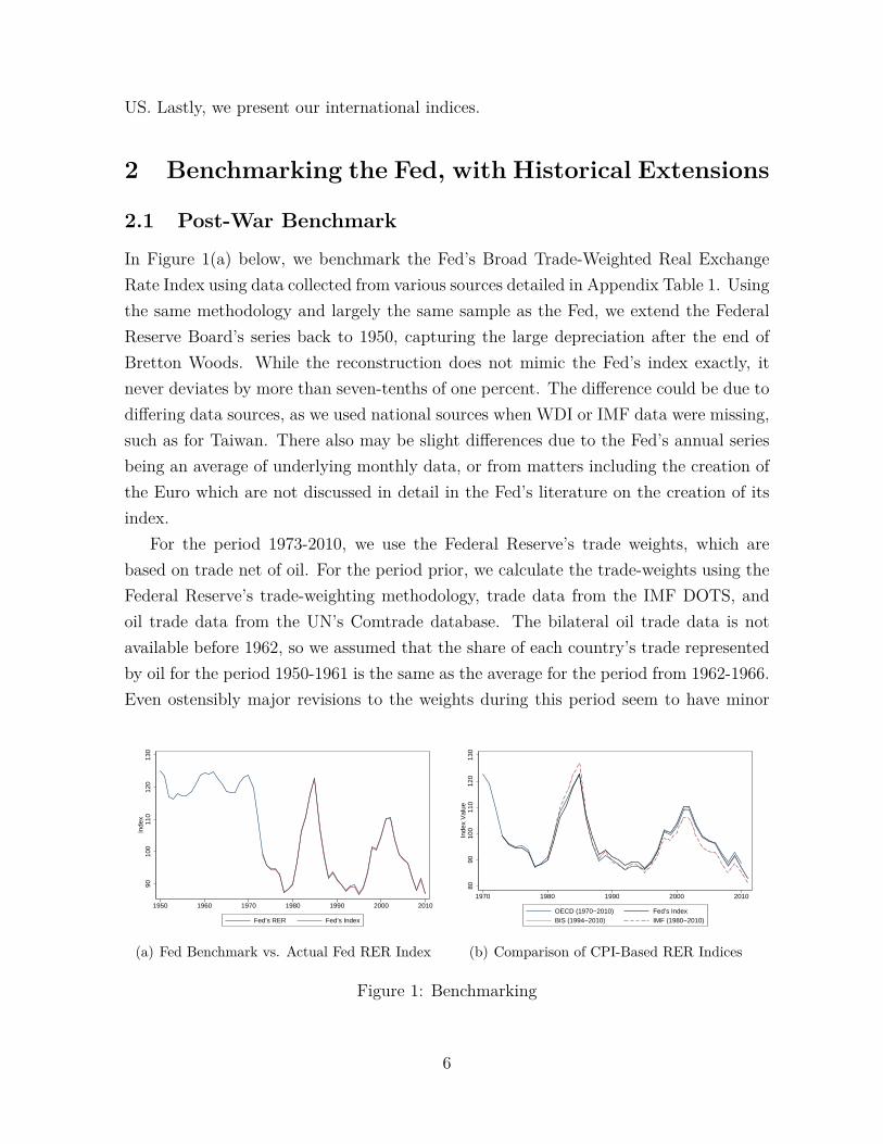
In Figure 1(a) below, we benchmark the Fed’s Broad Trade-Weighted Real ExchangeRate Index using data collected from various sources detailed in Appendix Table 1. Usingthe same methodology and largely the same sample as the Fed, we extend the FederalReserve Board’s series back to 1950, capturing the large depreciation after the end ofBretton Woods. While the reconstruction does not mimic the Fed’s index exactly, itnever deviates by more than seven-tenths of one percent. The difference could be due todiffering data sources, as we used national sources when WDI or IMF data were missing,such as for Taiwan. There also may be slight differences due to the Fed’s annual seriesbeing an average of underlying monthly data, or from matters including the creation ofthe Euro which are not discussed in detail in the Fed’s literature on the creation of itsindex.

For the period 1973-2010, we use the Federal Reserve’s trade weights, which arebased on trade net of oil. For the period prior, we calculate the trade-weights using theFederal Reserve’s trade-weighting methodology, trade data from the IMF DOTS, andoil trade data from the UN’s Comtrade database. The bilateral oil trade data is notavailable before 1962, so we assumed that the share of each country’s trade representedby oil for the period 1950-1961 is the same as the average for the period from 1962-1966.Even ostensibly major revisions to the weights during this period seem to have minor

9010

011

012

013

0In

dex

1950 1960 1970 1980 1990 2000 2010

Fed’s RER Fed’s Index

(a) Fed Benchmark vs. Actual Fed RER Index

8090

100

110

120

130

Inde

x V

alue

1970 1980 1990 2000 2010

OECD (1970−2010) Fed’s IndexBIS (1994−2010) IMF (1980−2010)

(b) Comparison of CPI-Based RER Indices

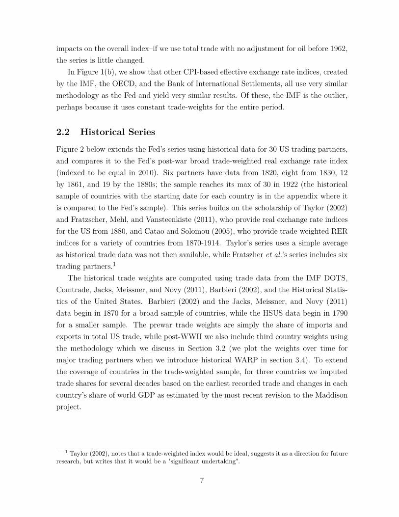
Figure 1: Benchmarking

6

impacts on the overall index–if we use total trade with no adjustment for oil before 1962,the series is little changed.

In Figure 1(b), we show that other CPI-based effective exchange rate indices, createdby the IMF, the OECD, and the Bank of International Settlements, all use very similarmethodology as the Fed and yield very similar results. Of these, the IMF is the outlier,perhaps because it uses constant trade-weights for the entire period.

2.2 Historical Series

Figure 2 below extends the Fed’s series using historical data for 30 US trading partners,and compares it to the Fed’s post-war broad trade-weighted real exchange rate index(indexed to be equal in 2010). Six partners have data from 1820, eight from 1830, 12by 1861, and 19 by the 1880s; the sample reaches its max of 30 in 1922 (the historicalsample of countries with the starting date for each country is in the appendix where itis compared to the Fed’s sample). This series builds on the scholarship of Taylor (2002)and Fratzscher, Mehl, and Vansteenkiste (2011), who provide real exchange rate indicesfor the US from 1880, and Catao and Solomou (2005), who provide trade-weighted RERindices for a variety of countries from 1870-1914. Taylor’s series uses a simple averageas historical trade data was not then available, while Fratszher et al.’s series includes sixtrading partners.1

The historical trade weights are computed using trade data from the IMF DOTS,Comtrade, Jacks, Meissner, and Novy (2011), Barbieri (2002), and the Historical Statis-tics of the United States. Barbieri (2002) and the Jacks, Meissner, and Novy (2011)data begin in 1870 for a broad sample of countries, while the HSUS data begin in 1790for a smaller sample. The prewar trade weights are simply the share of imports andexports in total US trade, while post-WWII we also include third country weights usingthe methodology which we discuss in Section 3.2 (we plot the weights over time formajor trading partners when we introduce historical WARP in section 3.4). To extendthe coverage of countries in the trade-weighted sample, for three countries we imputedtrade shares for several decades based on the earliest recorded trade and changes in eachcountry’s share of world GDP as estimated by the most recent revision to the Maddisonproject.

1 Taylor (2002), notes that a trade-weighted index would be ideal, suggests it as a direction for futureresearch, but writes that it would be a "significant undertaking".

7

100

120

140

160

180

200

1820 1830 1840 1850 1860 1870 1880 1890 1900 1910 1920 1930 1940 1950 1960 1970 1980 1990 2000 2010

Divisia Fed Broad Trade−Weighted RER

Figure 2: Historical Index Benchmarked to the Post-War Fed Index

3 Indexing Methods

3.1 A Review of Divisia vs. WARP

The Fed’s Broad Real Exchange Rate Index is computed as a weighted average of changesin underlying bilateral real exchange rate indices (this method is called “divisia”), wherethe base year value of each bilateral index is arbitrary. This is the appropriate con-struction of a nominal exchange rate index, as nominal exchange rates only containrelevant information when movements are plotted over time or when they are comparedto relative prices. Real exchange rates, however, do contain information, as they are anindication of the relative price of a basket of goods. As noted in Fahle, Marquez, andThomas (2008), this information is lost in the Fed’s approach, which is only informativewhen changes in the index values are plotted over time.

The Fed’s real exchange rate index is:

Idt = It−1 × ΠN(t)j=1 (

ej,tpt/pj,tej,t−1pt−1/pj,t−1

)wj,t . (3.1)

Where ej,t is the price of a dollar in terms of the currency of country j at time t,pt is the US consumer price index at time t, pj,t is the consumer price index of countryj at time t, N(t) is the number of countries in the basket, and wj,t is the trade weightof country j at time t. The base year is set at an arbitrary level, both for the indexand for each bilateral real exchange rate. The trade weight is a weighted average ofeach country’s share of imports, exports, and the degree of competition in third markets(trade weights are discussed later in this section).

8

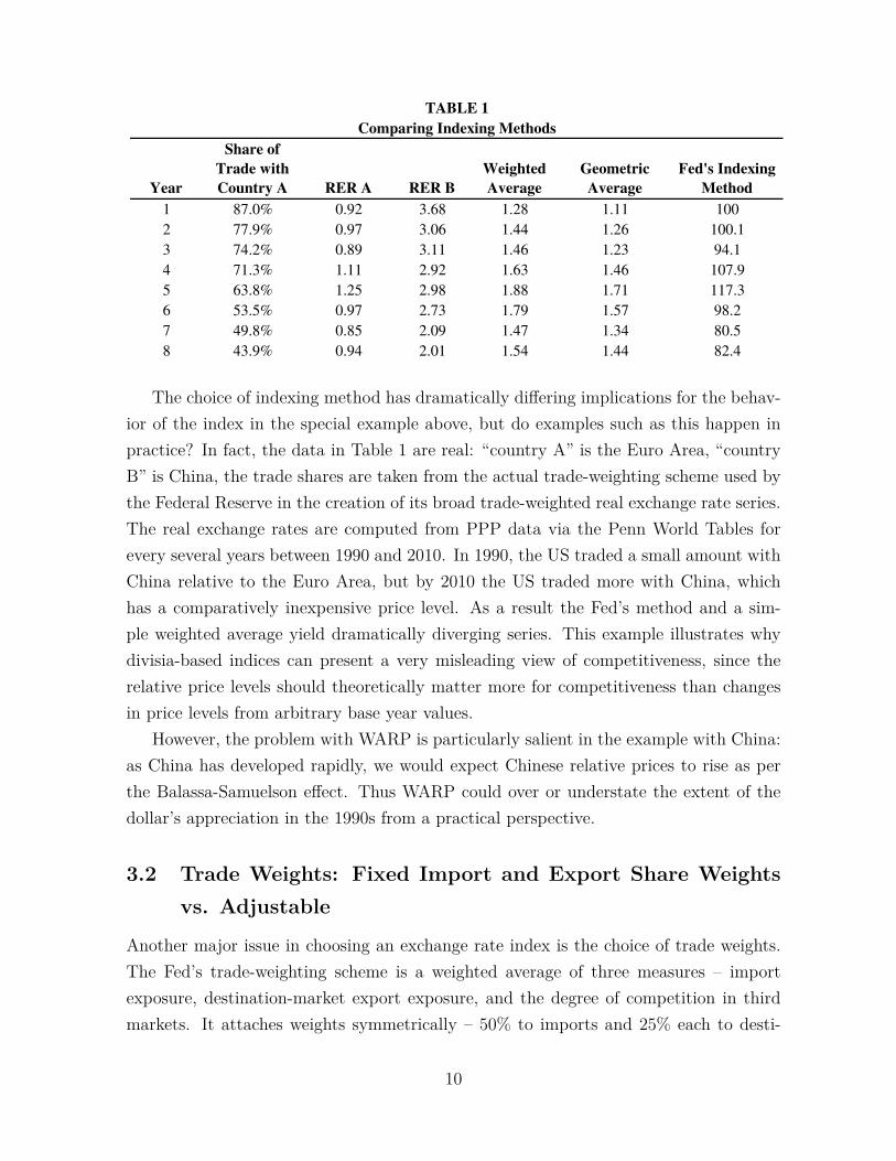
Note that while directional changes in real exchange rates will affect the index,changes in trade weights between countries with different levels of real exchange rateswill not. An issue arises when there is a shift in trade from countries with similar pricelevels to countries with very different price levels. Table 1 below describes a case inpoint. It compares several possible real exchange rate indices: a simple weighted av-erage, a geometric average (used by Fahle et. al. (2008)), and the Fed’s method. Inthis example, the bilateral real exchange rate for country A varies without trend, whilethe real exchange rate for country B appreciates substantially over the period relativeto the home country. Reflecting this, the Fed’s indexing method (also a geometric av-erage) reveals a substantial depreciation. However, at the beginning of the period, thehome country is trading mostly with country A (87% with country A implying 13% withcountry B), which has a similar price level, while at the end of the period a majority oftrade is with country B, which has a much lower price level. This is reflected in a simpleweighted average, or in the geometric average, which both show that by the end of theperiod the home country’s currency is much higher vs. a weighted average of its tradingpartners than it was at the beginning of the period.

In addition, the simple weighted average of real exchange rates has an intuitiveinterpration. For example, its value of 1.28 in the first year means that the price level is28% higher at home than in a weighted average of its trading partners, and about 20%lower than in the eighth year. By contrast, the value of 100 for year one using the Fed’smethod is just an arbitrary number with no economic meaning by itself.5

5Note that while the arithmetic average appears to be easier to intuit than the geometric average,which is less affected by extreme values, instead of using the price of goods in the US relative to countriesA and B, we could have used the prices of goods in those countries relative to the US. Inverting theresults using the arithmetic mean (which would also be the harmonic mean), and we would have verydifferent results. This is not an issue with the geometric mean. Otherwise we might favor the arithmeticmean, since from a competitive perspective, having a currency overvalued by 20% with respect to onetrading partner is probably more damaging than having your currency overvalued by 1% with respect to20 countries. The arithmetic average will yield the same results for these two cases, while the geometricaverage will yield a lower value for the first scenario.

9

Year

Share of

Trade with

Country A RER A RER B

Weighted

Average

Geometric

Average

Fed's Indexing

Method

1 87.0% 0.92 3.68 1.28 1.11 100

2 77.9% 0.97 3.06 1.44 1.26 100.1

3 74.2% 0.89 3.11 1.46 1.23 94.1

4 71.3% 1.11 2.92 1.63 1.46 107.9

5 63.8% 1.25 2.98 1.88 1.71 117.3

6 53.5% 0.97 2.73 1.79 1.57 98.2

7 49.8% 0.85 2.09 1.47 1.34 80.5

8 43.9% 0.94 2.01 1.54 1.44 82.4

Comparing Indexing Methods

TABLE 1

The choice of indexing method has dramatically differing implications for the behav-ior of the index in the special example above, but do examples such as this happen inpractice? In fact, the data in Table 1 are real: “country A” is the Euro Area, “countryB” is China, the trade shares are taken from the actual trade-weighting scheme used bythe Federal Reserve in the creation of its broad trade-weighted real exchange rate series.The real exchange rates are computed from PPP data via the Penn World Tables forevery several years between 1990 and 2010. In 1990, the US traded a small amount withChina relative to the Euro Area, but by 2010 the US traded more with China, whichhas a comparatively inexpensive price level. As a result the Fed’s method and a sim-ple weighted average yield dramatically diverging series. This example illustrates whydivisia-based indices can present a very misleading view of competitiveness, since therelative price levels should theoretically matter more for competitiveness than changesin price levels from arbitrary base year values.

However, the problem with WARP is particularly salient in the example with China:as China has developed rapidly, we would expect Chinese relative prices to rise as perthe Balassa-Samuelson effect. Thus WARP could over or understate the extent of thedollar’s appreciation in the 1990s from a practical perspective.

3.2 Trade Weights: Fixed Import and Export Share Weightsvs. Adjustable

Another major issue in choosing an exchange rate index is the choice of trade weights.The Fed’s trade-weighting scheme is a weighted average of three measures – importexposure, destination-market export exposure, and the degree of competition in thirdmarkets. It attaches weights symmetrically – 50% to imports and 25% each to desti-

10

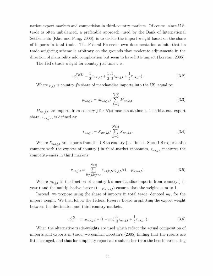
nation export markets and competition in third-country markets. Of course, since U.S.trade is often unbalanced, a preferable approach, used by the Bank of InternationalSettlements (Klau and Fung, 2006), is to decide the import weight based on the shareof imports in total trade. The Federal Reserve’s own documentation admits that itstrade-weighting scheme is arbitrary on the grounds that moderate adjustments in thedirection of plausibility add complication but seem to have little impact (Loretan, 2005).

The Fed’s trade weight for country j at time t is:

wFEDj,t = 12µus,j,t + 1

2(12εus,j,t + 1

2τus,j,t). (3.2)

Where µj,t is country j’s share of merchandise imports into the US, equal to:

µus,j,t = Mus,j,t/

N(t)∑k=1

Mus,k,t. (3.3)

Mus,j,t are imports from country j for N(t) markets at time t. The bilateral exportshare, εus,j,t, is defined as:

εus,j,t = Xus,j,t/

N(t)∑k=1

Xus,k,t. (3.4)

Where Xus,j,t are exports from the US to country j at time t. Since US exports alsocompete with the exports of country j in third-market economies, τus,j,t measures thecompetitiveness in third markets:

τus,j,t =N(t)∑

k 6=j,k 6=usεus,k,tµk,j,t/(1− µk,us,t). (3.5)

Where µk,j,t is the fraction of country k’s merchandise imports from country j inyear t and the multiplicative factor (1− µk,us,t) ensures that the weights sum to 1.

Instead, we propose using the share of imports in total trade, denoted mt, for theimport weight. We then follow the Federal Reserve Board in splitting the export weightbetween the destination and third-country markets.

wAltj,t = mtµus,j,t + (1−mt)(12εus,j,t + 1

2τus,j,t). (3.6)

When the alternative trade-weights are used which reflect the actual composition ofimports and exports in trade, we confirm Loretan’s (2005) finding that the results arelittle-changed, and thus for simplicity report all results other than the benchmarks using

11

these adjusted trade weights.A very prudent second critique is that the Fed’s trade-weights measure trade in

goods rather than trade in value-added. Bems and Johnson (2012) show that for theUS, the differences in trade shares using value-added seems to make little difference.6

For example, they find that the US trade share with China shrinks by just -.2% in 2005.A third critique was mounted by Ho (2012), who proposed using GDP weights instead

of trade weights, and found some support that in many cases (although not for the US),the GDP weights do a better job of explaining real exports using cointegration analysis.Thus, following Ho (2012), we also provide GDP-weighted versions of our index, whichactually differ more substantially than trade-weighted indices for the class of weighted-average relative indices proposed here.

3.3 Post-War WARP for the United States

Weighted average relative prices (WARP) are computed as a geometric weighted averageusing trade-weights, wj,t, of the nominal exchange rate, ej,t, divided by purchasing powerparity, PPPj,t:

IWARPt =

N(t)∏j=1

( ej,tPPPj,t

)wj,t =N(t)∏j=1

(RERj,t

)wj,t. (3.7)

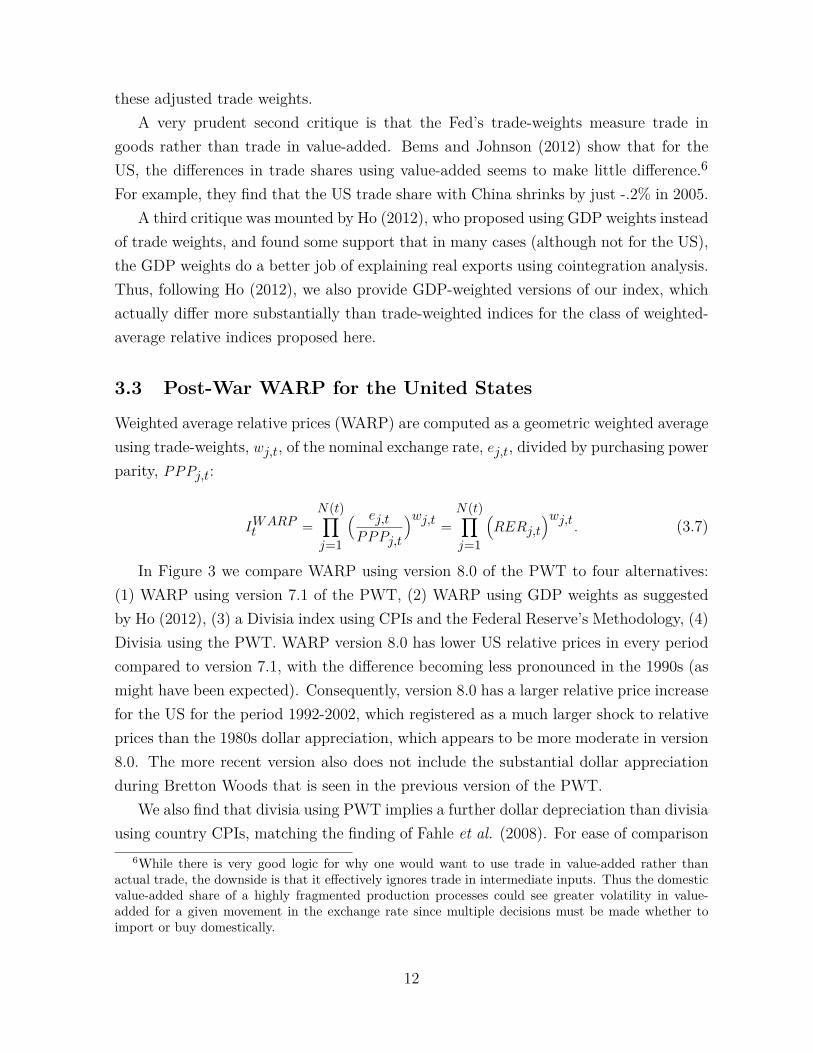
In Figure 3 we compare WARP using version 8.0 of the PWT to four alternatives:(1) WARP using version 7.1 of the PWT, (2) WARP using GDP weights as suggestedby Ho (2012), (3) a Divisia index using CPIs and the Federal Reserve’s Methodology, (4)Divisia using the PWT. WARP version 8.0 has lower US relative prices in every periodcompared to version 7.1, with the difference becoming less pronounced in the 1990s (asmight have been expected). Consequently, version 8.0 has a larger relative price increasefor the US for the period 1992-2002, which registered as a much larger shock to relativeprices than the 1980s dollar appreciation, which appears to be more moderate in version8.0. The more recent version also does not include the substantial dollar appreciationduring Bretton Woods that is seen in the previous version of the PWT.

We also find that divisia using PWT implies a further dollar depreciation than divisiausing country CPIs, matching the finding of Fahle et al. (2008). For ease of comparison

6While there is very good logic for why one would want to use trade in value-added rather thanactual trade, the downside is that it effectively ignores trade in intermediate inputs. Thus the domesticvalue-added share of a highly fragmented production processes could see greater volatility in value-added for a given movement in the exchange rate since multiple decisions must be made whether toimport or buy domestically.

12

.81

1.2

1.4

1.6

Inde

x

1950 1960 1970 1980 1990 2000 2010

WARP v8.0 Divisia using PWTWARP v7.1 GDP−Weighted WARPDivisia (CPI)

Figure 3: WARPs vs. Divisias

the Divisia using the CPI (essentially the Fed’s series) is multiplied by a scaling factor sothat it begins at the same level as the WARP in 1973, which gives the Fed’s series baseyear an intuitive economic meaning – in 1973, the U.S. price level was about 30% higherthan a (geometric) weighted average of U.S. trading partners. WARP v8.0 approximatesthe Fed’s index up until the dollar appreciation in the 1980s, when it shows less of anappreciation (this was much less apparent in version 7.1 of the PWT). Since the early1990s, the WARP index reveals a much larger appreciation relative to the Fed’s index,appreciating 26% more from 1990-2002. From 1990-2011 WARP appreciated by 12.9%versus a 9% depreciation according to divisia. The divisia index computed using thePPP of output from PWT v8.0 is very similar to that using expenditure-based PPP,and also very similar to using World Bank GDP deflators, as used in the constructionof value-added exchange rates (Bems and Johnson, 2012, and Bayoumi et al., 2013).

3.4 A WARPed View of US Real Exchange Rate History

This paper is the first to plot weighted average relative prices for the U.S. before 1970,adding 150 years of data to the Fahle et. al. (2008) series. How does WARP changeour view of history? The major difference is that in the WARP series, the price level

13

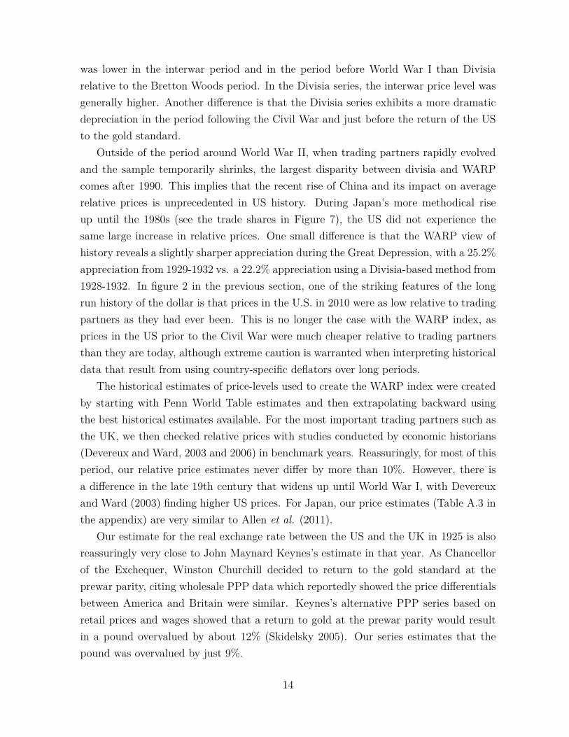
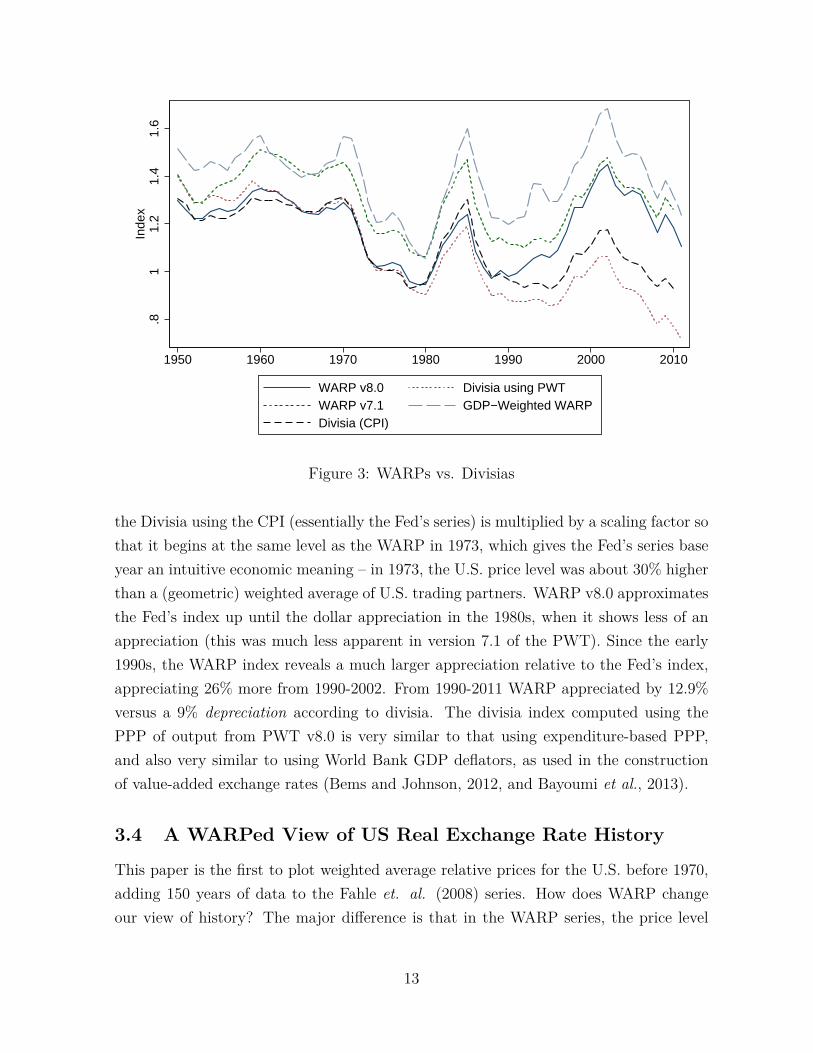
was lower in the interwar period and in the period before World War I than Divisiarelative to the Bretton Woods period. In the Divisia series, the interwar price level wasgenerally higher. Another difference is that the Divisia series exhibits a more dramaticdepreciation in the period following the Civil War and just before the return of the USto the gold standard.

Outside of the period around World War II, when trading partners rapidly evolvedand the sample temporarily shrinks, the largest disparity between divisia and WARPcomes after 1990. This implies that the recent rise of China and its impact on averagerelative prices is unprecedented in US history. During Japan’s more methodical riseup until the 1980s (see the trade shares in Figure 7), the US did not experience thesame large increase in relative prices. One small difference is that the WARP view ofhistory reveals a slightly sharper appreciation during the Great Depression, with a 25.2%appreciation from 1929-1932 vs. a 22.2% appreciation using a Divisia-based method from1928-1932. In figure 2 in the previous section, one of the striking features of the longrun history of the dollar is that prices in the U.S. in 2010 were as low relative to tradingpartners as they had ever been. This is no longer the case with the WARP index, asprices in the US prior to the Civil War were much cheaper relative to trading partnersthan they are today, although extreme caution is warranted when interpreting historicaldata that result from using country-specific deflators over long periods.

The historical estimates of price-levels used to create the WARP index were createdby starting with Penn World Table estimates and then extrapolating backward usingthe best historical estimates available. For the most important trading partners such asthe UK, we then checked relative prices with studies conducted by economic historians(Devereux and Ward, 2003 and 2006) in benchmark years. Reassuringly, for most of thisperiod, our relative price estimates never differ by more than 10%. However, there isa difference in the late 19th century that widens up until World War I, with Devereuxand Ward (2003) finding higher US prices. For Japan, our price estimates (Table A.3 inthe appendix) are very similar to Allen et al. (2011).

Our estimate for the real exchange rate between the US and the UK in 1925 is alsoreassuringly very close to John Maynard Keynes’s estimate in that year. As Chancellorof the Exchequer, Winston Churchill decided to return to the gold standard at theprewar parity, citing wholesale PPP data which reportedly showed the price differentialsbetween America and Britain were similar. Keynes’s alternative PPP series based onretail prices and wages showed that a return to gold at the prewar parity would resultin a pound overvalued by about 12% (Skidelsky 2005). Our series estimates that thepound was overvalued by just 9%.

14

.81

1.2

1.4

1.6

1.8

1820 1830 1840 1850 1860 1870 1880 1890 1900 1910 1920 1930 1940 1950 1960 1970 1980 1990 2000 2010

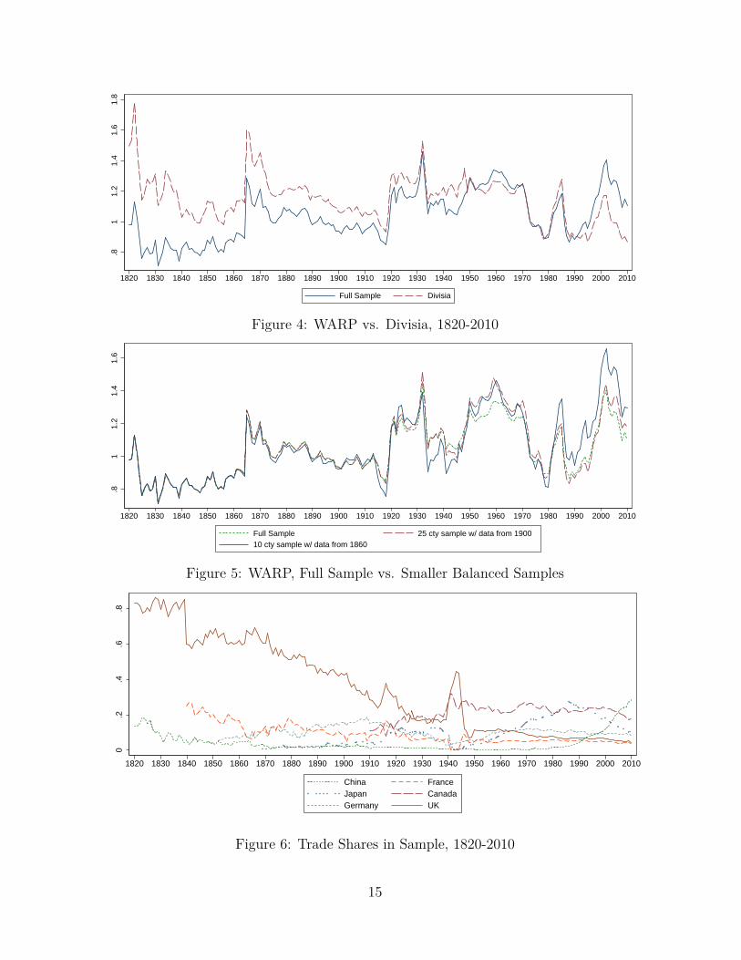
Full Sample Divisia

Figure 4: WARP vs. Divisia, 1820-2010

.81

1.2

1.4

1.6

1820 1830 1840 1850 1860 1870 1880 1890 1900 1910 1920 1930 1940 1950 1960 1970 1980 1990 2000 2010

Full Sample 25 cty sample w/ data from 190010 cty sample w/ data from 1860

Figure 5: WARP, Full Sample vs. Smaller Balanced Samples

0.2

.4.6

.8

1820 1830 1840 1850 1860 1870 1880 1890 1900 1910 1920 1930 1940 1950 1960 1970 1980 1990 2000 2010

China FranceJapan CanadaGermany UK

Figure 6: Trade Shares in Sample, 1820-2010

15

4 Balassa-Samuelson Productivity Adjustment

4.1 Constant Coefficient Balassa-Samuelson

TheWARP index, while likely preferable to the Fed’s series for the purposes of mesauringthe competitiveness of U.S. goods and services in international trade (Loretan, 2005),may not be the optimal method since it only factors in prices and not productivity.The Balassa-Samuelson (or the “Penn”) effect implies that if traded sectors have fasterproductivity growth, then the productivity differentials between rich and poor countrieswill be greater in the tradable sectors. In each country wages in the non-traded sectorwill be bid to equality with wages in the traded sector, and hence non-traded prices inless developed countries will be lower. What matters, then, is the level of real exchangerates relative to some measure of productivity, such as per capita GDP. To correct forthe Balassa-Samuelson effect, we propose the following index:

IBSWARPt =

N(t)∏j=1

(exp(εUS,t − εj,t))wj,t . (4.1)

Where wj,t are trade weights, and εUS,t and εj,t are the residuals for the US andcountry j from the Balassa-Samuelson regression (used by Rodrik, 2008):

lnRERj,t = α + β ∗ lnRGDPPCj,t +2010∑t=1950

ft + εj,t. (4.2)

Where RERj,t is the real exchange rate vs. the dollar for each country in the world(in this case, the RER is defined such that larger numbers indicate a higher price levelfor country j relative to the US), RGDPPCj,t is the real GDP per capita, and ft areyear fixed effects. The regression yields a coefficient on log GDP per capita of .133for 186 countries for the period 1973-2011 (a smaller, balanced sample yields a similarestimate). The residual εUS,t has a simple economic meaning – it tells us how over orunder-valued the dollar is relative to where it should be based on US GDP per capita.This number is then adjusted based on the relative valuation of US trading partners. Ifthe US and each of its trading partners were to lie on the Balassa-Samuelson regressionline, then the index would be zero, indicating that the dollar is fairly valued. Manypapers, such as Rodrik (2008), which study the impact of exchange rates on growth,use the Balassa-Samuelson residual rather than a trade-weighted average of a country’sresidual differenced with its trading partners.

One can see the relationship between Divisia, WARP, and BS-WARP by totally

16

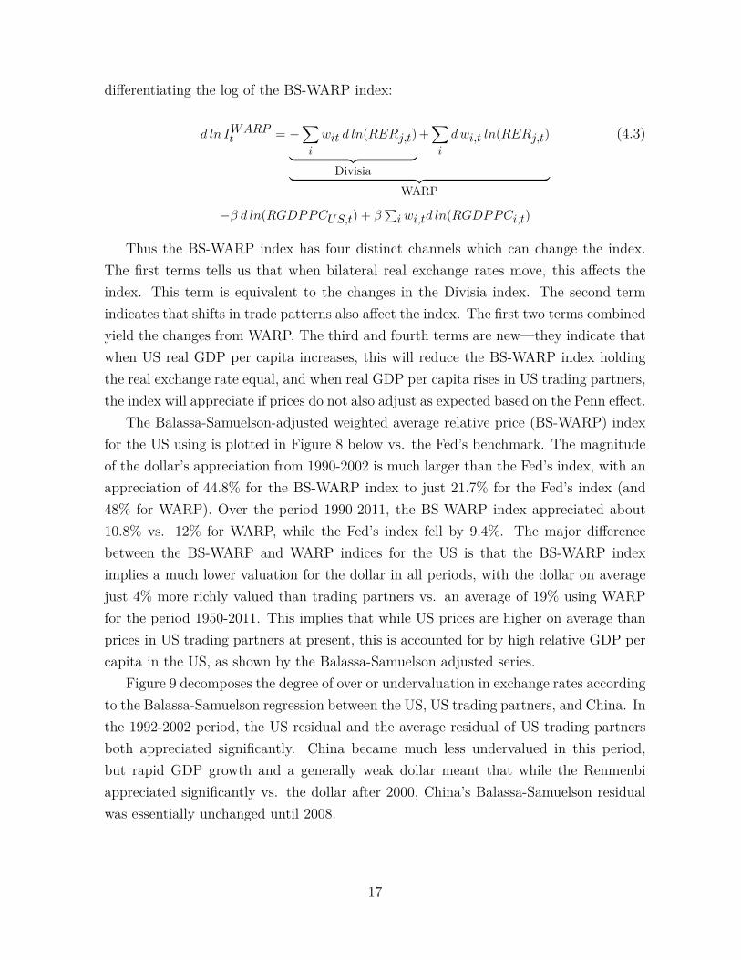
differentiating the log of the BS-WARP index:

d ln IWARPt = −

∑i

wit d ln(RERj,t)︸ ︷︷ ︸Divisia

+∑i

dwi,t ln(RERj,t)

︸ ︷︷ ︸WARP

(4.3)

−β d ln(RGDPPCUS,t) + β∑i wi,td ln(RGDPPCi,t)

Thus the BS-WARP index has four distinct channels which can change the index.The first terms tells us that when bilateral real exchange rates move, this affects theindex. This term is equivalent to the changes in the Divisia index. The second termindicates that shifts in trade patterns also affect the index. The first two terms combinedyield the changes from WARP. The third and fourth terms are new—they indicate thatwhen US real GDP per capita increases, this will reduce the BS-WARP index holdingthe real exchange rate equal, and when real GDP per capita rises in US trading partners,the index will appreciate if prices do not also adjust as expected based on the Penn effect.

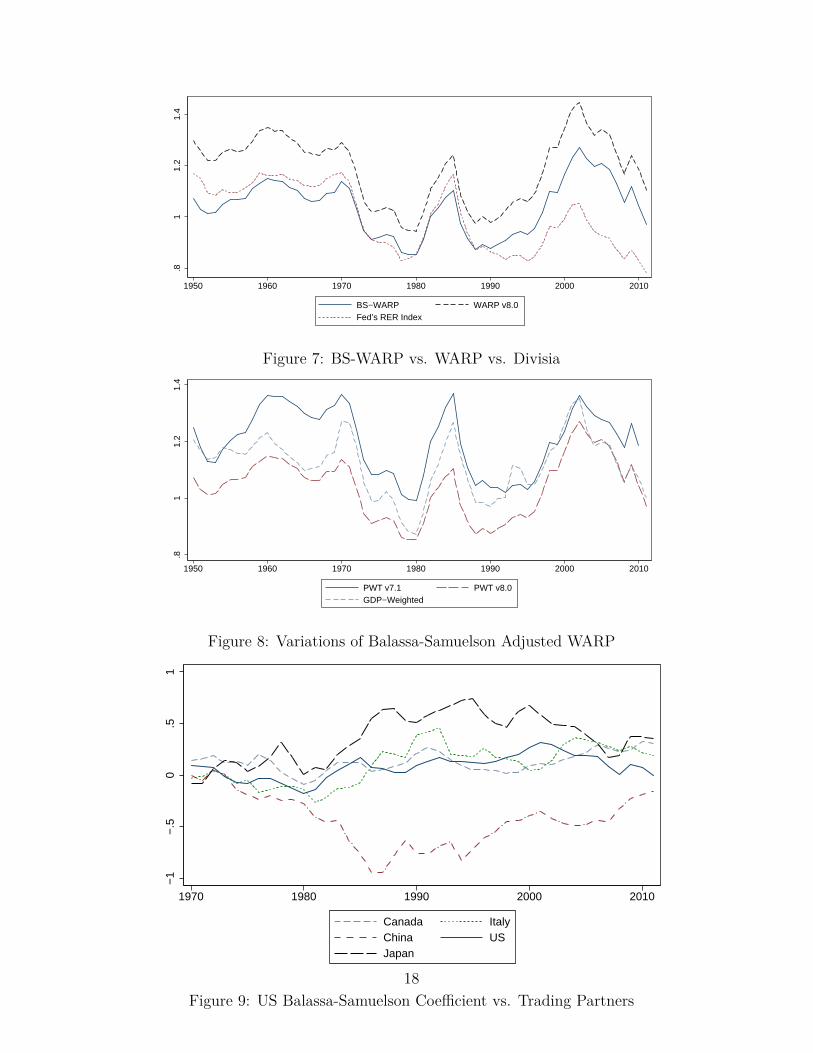
The Balassa-Samuelson-adjusted weighted average relative price (BS-WARP) indexfor the US using is plotted in Figure 8 below vs. the Fed’s benchmark. The magnitudeof the dollar’s appreciation from 1990-2002 is much larger than the Fed’s index, with anappreciation of 44.8% for the BS-WARP index to just 21.7% for the Fed’s index (and48% for WARP). Over the period 1990-2011, the BS-WARP index appreciated about10.8% vs. 12% for WARP, while the Fed’s index fell by 9.4%. The major differencebetween the BS-WARP and WARP indices for the US is that the BS-WARP indeximplies a much lower valuation for the dollar in all periods, with the dollar on averagejust 4% more richly valued than trading partners vs. an average of 19% using WARPfor the period 1950-2011. This implies that while US prices are higher on average thanprices in US trading partners at present, this is accounted for by high relative GDP percapita in the US, as shown by the Balassa-Samuelson adjusted series.

Figure 9 decomposes the degree of over or undervaluation in exchange rates accordingto the Balassa-Samuelson regression between the US, US trading partners, and China. Inthe 1992-2002 period, the US residual and the average residual of US trading partnersboth appreciated significantly. China became much less undervalued in this period,but rapid GDP growth and a generally weak dollar meant that while the Renmenbiappreciated significantly vs. the dollar after 2000, China’s Balassa-Samuelson residualwas essentially unchanged until 2008.

17

.81

1.2

1.4

1950 1960 1970 1980 1990 2000 2010

BS−WARP WARP v8.0Fed’s RER Index

Figure 7: BS-WARP vs. WARP vs. Divisia

.81

1.2

1.4

1950 1960 1970 1980 1990 2000 2010

PWT v7.1 PWT v8.0GDP−Weighted

Figure 8: Variations of Balassa-Samuelson Adjusted WARP

−1

−.5

0.5

1

1970 1980 1990 2000 2010

Canada ItalyChina USJapan

Figure 9: US Balassa-Samuelson Coefficient vs. Trading Partners18

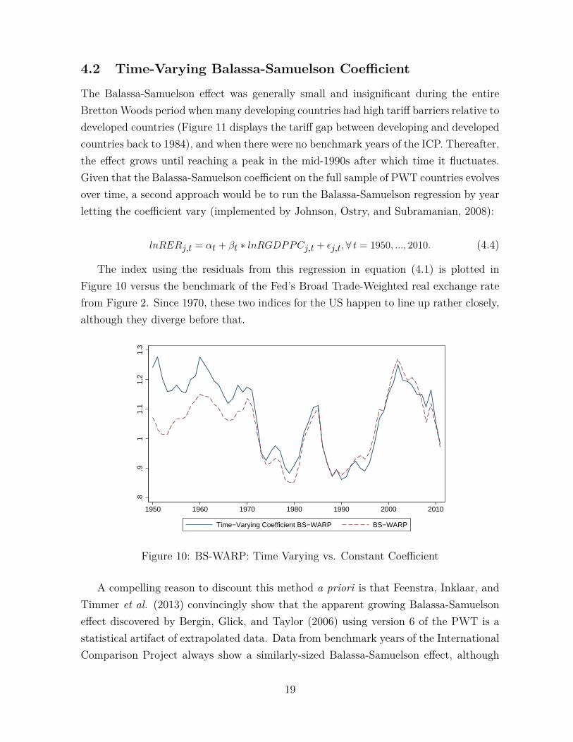
4.2 Time-Varying Balassa-Samuelson Coefficient

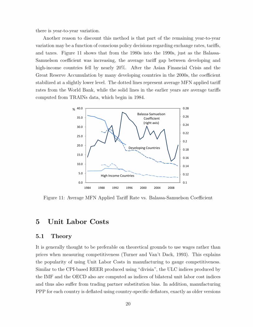
The Balassa-Samuelson effect was generally small and insignificant during the entireBrettonWoods period when many developing countries had high tariff barriers relative todeveloped countries (Figure 11 displays the tariff gap between developing and developedcountries back to 1984), and when there were no benchmark years of the ICP. Thereafter,the effect grows until reaching a peak in the mid-1990s after which time it fluctuates.Given that the Balassa-Samuelson coefficient on the full sample of PWT countries evolvesover time, a second approach would be to run the Balassa-Samuelson regression by yearletting the coefficient vary (implemented by Johnson, Ostry, and Subramanian, 2008):

lnRERj,t = αt + βt ∗ lnRGDPPCj,t + εj,t,∀ t = 1950, ..., 2010. (4.4)

The index using the residuals from this regression in equation (4.1) is plotted inFigure 10 versus the benchmark of the Fed’s Broad Trade-Weighted real exchange ratefrom Figure 2. Since 1970, these two indices for the US happen to line up rather closely,although they diverge before that.

.8.9

11.

11.

21.

3

1950 1960 1970 1980 1990 2000 2010

Time−Varying Coefficient BS−WARP BS−WARP

Figure 10: BS-WARP: Time Varying vs. Constant Coefficient

A compelling reason to discount this method a priori is that Feenstra, Inklaar, andTimmer et al. (2013) convincingly show that the apparent growing Balassa-Samuelsoneffect discovered by Bergin, Glick, and Taylor (2006) using version 6 of the PWT is astatistical artifact of extrapolated data. Data from benchmark years of the InternationalComparison Project always show a similarly-sized Balassa-Samuelson effect, although

19

there is year-to-year variation.Another reason to discount this method is that part of the remaining year-to-year

variation may be a function of conscious policy decisions regarding exchange rates, tariffs,and taxes. Figure 11 shows that from the 1980s into the 1990s, just as the Balassa-Samuelson coefficient was increasing, the average tariff gap between developing andhigh-income countries fell by nearly 20%. After the Asian Financial Crisis and theGreat Reserve Accumulation by many developing countries in the 2000s, the coefficientstabilized at a slightly lower level. The dotted lines represent average MFN applied tariffrates from the World Bank, while the solid lines in the earlier years are average tariffscomputed from TRAINs data, which begin in 1984.

0.2

0.22

0.24

0.26

0.28

25.0

30.0

35.0

40.0%

Balassa-Samuelson

Coefficient

(right axis)

0.1

0.12

0.14

0.16

0.18

0.2

0.0

5.0

10.0

15.0

20.0

1984 1988 1992 1996 2000 2004 2008

Developing Countries

High Income Countries

Figure 11: Average MFN Applied Tariff Rate vs. Balassa-Samuelson Coefficient

5 Unit Labor Costs

5.1 Theory

It is generally thought to be preferable on theoretical grounds to use wages rather thanprices when measuring competitiveness (Turner and Van’t Dack, 1993). This explainsthe popularity of using Unit Labor Costs in manufacturing to gauge competitiveness.Similar to the CPI-based REER produced using “divisia”, the ULC indices produced bythe IMF and the OECD also are computed as indices of bilateral unit labor cost indicesand thus also suffer from trading partner substitution bias. In addition, manufacturingPPP for each country is deflated using country-specific deflators, exactly as older versions

20

of the Penn World Tables, which predated version 8.0, were computed. The series wepropose is thus a simple Weighted Average of Relative Unit Labor Costs (WARULC)rather than of the unit labor cost indices – analagous to WARP. In our series, wecompute manufacturing PPP using PWT v8.0 methodology described in Feenstra etal. (2013). When we also expand the sample to include developing countries such asChina and time-varying trade-weights, the differences in the underlying index becomesubstantial. This is due to China’s systematically lower unit labor costs and growingweight in manufacturing trade over time.

The IMF’s RULC index, documented by Desruelle and Zanello (1997), is computedas:

IRULCUS,t =∏i=1

(CIUSRIUSCIi R

Ii

)wi (5.1)

Where CIi is the normalized unit labor cost index for country i, computed as theratio of nominal sectoral wages to real productivity, Ri is the nominal exchange rateindex, and wi are the time invariant trade weights. One intuitive proposed alternativespecification would be to replace the unit labor cost indices with the same unindexed unitlabor costs, and actual nominal exchange rates. However, the relative unit labor costsusing deflated real productivity will depend on the base year used to deflate productivity.To circumvent this problem, we convert nominal productivity into dollars using the PPPexchange rate conversion for the manufactuing sector, following the method Golub andCeglowski (2007) implement for just the US and China, while converting nominal wagesinto dollars at the nominal exchange rate.7

For this index, we used OECD data created specifically for the construction of ULCindices where available, and supplemented this with data from the BLS, the Chinesegovernment, the World Bank’s WDI, and UNIDOs. The manufacturing PPP data forbenchmark years come from the relevant ICP headings and were computed using PWTmethodology (described in Section 3 of Feenstra et al. 2013), and were interpolatedin the intervening years using country growth rates. The methodology and formulasfor the interpolation were also borrowed from Feenstra et al. (2013). E.g., after thelast benchmark year in 2005, the series are extended based on country growth rates for

7Since the index is of relative unit labor costs, and as Rudiger Dornbusch used to say, two nominalsmake a real, the use of nominal wages converted at exchange rates is not problematic.

21

country i:

Pi,2006 = P ICPi,2005 ∗Pi,deflatori,2006

Pi,deflatori,2005

, (5.2)

where P i,deflatori,t is the country-specific deflator at time t.For the years in between ICP benchmarks, a weighted average was used. For example,

for the years between 1996 and 2005, the formula is:

Pi,t = P ICPi,1996 ∗Pi,deflatori,t

Pi,deflatori,1996

( 2005− t2005− 1996

)+ P ICPi,2005 ∗

Pi,deflatori,t

Pi,deflatori,2005

( t− 19962005− 1996

). (5.3)

Data on manufacturing trade to create trade weights ωi,t is computed from bilateralmanufacturing data at the SITC 4 level from Feenstra et al. (2005), and with updateddata through 2008 via direct communication with Feenstra. Manufacturing trade datafrom 2009 and 2010 were taken from the OECD.

The weighted average relative unit labor cost index (WARULC) is computed as:

IWARULCUS,t =

∏i=1

(CUS,tCi,t

)ωi,t =∏i=1

( wUS,teUS,t/

YUS,tPPPUS,t

wi,tei,t

/Yi,t

PPPi,t

)ωi,t. (5.4)

Where wi,t are manufacturing wages of country i at time t, ei,t is the nominal ex-change rate to convert to dollars, Yi,t is manufacturing production, and is divided byPPP for the manufacturing sector. Thus the C’s here are unit labor costs rather thanindexes of unit labor costs.

5.2 Data

When the Weighted Average Relative Unit Labor Cost (WARULC) index is comparedwith the official IMF RULC index (indexed to start at the same value in 1975) and anindex using our data but the IMF’s index-of-indices method, the results are strikinglydifferent, with the difference much larger than the disparity between WARP and Divisiacomputed with CPIs. The series are roughly similarly until the late 1980s, but by 2001,the WARULC index is 32% higher than the IMF’s index, and 44% higher in 2008. TheIMF benchmark index constructed here using the IMF’s index-of-index method is similarto the IMF’s index, despite the fact that we used time-varying manufacturing tradeweights, a larger sample of countries (including China), and we compute manufacturing

22

value-added using PPP. The IMF instead uses an index of real output measured inthe home currency, and so it is striking that the benchmark is similar to both theIMF and the OECD indexes (the latter is not shown but also similar). We have alsoplotted a WARULC series which uses manufacturing PPP computed using only a singlebenchmark year and country deflators (short maroon dashes in figure 12). The serieswithout multiple benchmarks displays a downward trend relative to our preferred serieswith multiple benchmarks.

.51

1.5

2

1970 1975 1980 1985 1990 1995 2000 2005 2010

IMF RULC RULC, IMF BenchmarkWARULC WARULC (mult. benchmarks)

Figure 12: IMF Method vs. WARULC

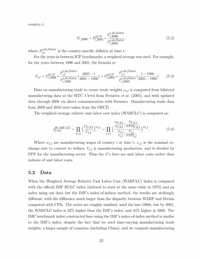
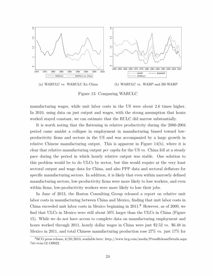
And, just as with WARP, the difference between WARULC and the IMF’s index islargely China, as evidenced in Figure 13(a). In 13(b) we compare WARP, BS-WARP,and WARULC, and find that they are all broadly similar, with the exception being thatthe WARULC index displays a sharper depreciation after 2001.

Figure 14 details estimates of relative hourly productivity, wages, and ULCs for theUS relative to China. These results are very similar to Golub and Ceglowski (2012) forthe 1998-2009 period. The ratio of hourly wages has indeed fallen dramatically since theearly 1990s, but not much more quickly than the convergence in productivity. Relativeunit labor costs spiked in the late 1990s and early 2000s, during the collapse of USmanufacturing employment concentrated heavily in China-competing industries. As of2009, US manufacturing wages were still approximately 20 times larger than Chinese

23

.81

1.2

1.4

1.6

1970 1975 1980 1985 1990 1995 2000 2005 2010

WARULC WARULC ex−China

(a) WARULC vs. WARULC Ex China

.81

1.2

1.4

1.6

1950 1955 1960 1965 1970 1975 1980 1985 1990 1995 2000 2005 2010

WARP BSWARPWARULC

(b) WARULC vs. WARP and BS-WARP

Figure 13: Comparing WARULC

manufacturing wages, while unit labor costs in the US were about 2.6 times higher.In 2010, using data on just output and wages, with the strong assumption that hoursworked stayed constant, we can estimate that the RULC did narrow substantially.

It is worth noting that the flattening in relative productivity during the 2000-2004period came amidst a collapse in employment in manufacturing biased toward low-productivity firms and sectors in the US and was accompanied by a large growth inrelative Chinese manufacturing output. This is apparent in Figure 14(b), where it isclear that relative manufacturing output per capita for the US vs. China fell at a steadypace during the period in which hourly relative output was stable. One solution tothis problem would be to do ULCs by sector, but this would require at the very leastsectoral output and wage data for China, and also PPP data and sectoral deflators forspecific manufacturing sectors. In addition, it is likely that even within narrowly definedmanufacturing sectors, low-productivity firms were more likely to lose workers, and evenwithin firms, low-productivity workers were more likely to lose their jobs.

In June of 2013, the Boston Consulting Group released a report on relative unitlabor costs in manufacturing between China and Mexico, finding that unit labor costs inChina exceeded unit labor costs in Mexico beginning in 2011.8 However, as of 2009, wefind that ULCs in Mexico were still about 50% larger than the ULCs in China (Figure15). While we do not have access to complete data on manufacturing employment andhours worked through 2011, hourly dollar wages in China were just $2.52 vs. $6.48 inMexico in 2011, and total Chinese manufacturing production rose 27% vs. just 17% for

8BCG press release, 6/28/2013, available here: http://www.bcg.com/media/PressReleaseDetails.aspx?id=tcm:12-139022.

24

22.

53

3.5

020

4060

8010

0

1975 1980 1985 1990 1995 2000 2005 2010

Extended Rel. Output US Rel. Hourly OutputRelative Hourly Wage Extended RULCRULC (right axis)

(a) Relative Wages and Productivity

510

1520

2530

1975 1980 1985 1990 1995 2000 2005 2010

Rel. Man. Output per capita Rel. Man. Output per hour

(b) Output vs. Productivity

Figure 14: US vs. China

.1.2

.3.4

.5

1970 1980 1990 2000 2010

Mexico ULC extension MexicoChina ULC extension China

Figure 15: ULCs, Mexico vs. China

Mexico from 2009-2011. If there was no change in relative hours worked, admittedlya very strong assumption, then ULCs did converge a bit between 2009 and 2011, butMexican ULCs were still roughly 33% higher than Chinese ULCs in 2011. Thus Mexicanmanufacturing workers, in the aggregate, are still substantially more productive thantheir Chinese counterparts, although also better paid relative to productivity.

6 Adjusting for Domestic Competition

In trying to take the indices computed in this paper to the data, or in order to makecomparisons over different countries (as in the next section) or over different epochs,another problem emerges. Any given producer of a tradable good would theoreticallybe more exposed to exchange rate movements if located in a small open economy versusa large economy with less trade exposure. A US manufacturer in 1950 mostly competed

25

with other manufacturers located in the US, was likely to export little, and on averagewould not have been much affected by a 10% appreciation of the dollar. Thus, an al-ternative index operating from the perspective of an individual firm should include aweight for home-country competition, for which the real exchange rate is always one.Firms located in countries with less trade as a share of output would thereby system-atically experience less variation in their real exchange rate indices. Thus since Italytrades much more than the US as a share of GDP, in large part because Italy is muchsmaller, we would expect its real exchange rate to rise by less due to increased tradewith China, since even if China traded as much with Italy as with the US as a share ofGDP, its share in Italian trade would be much smaller.

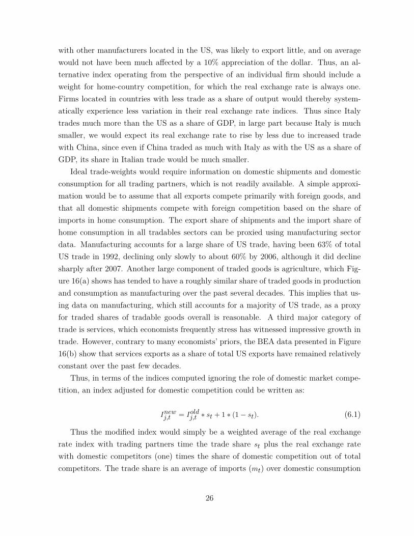
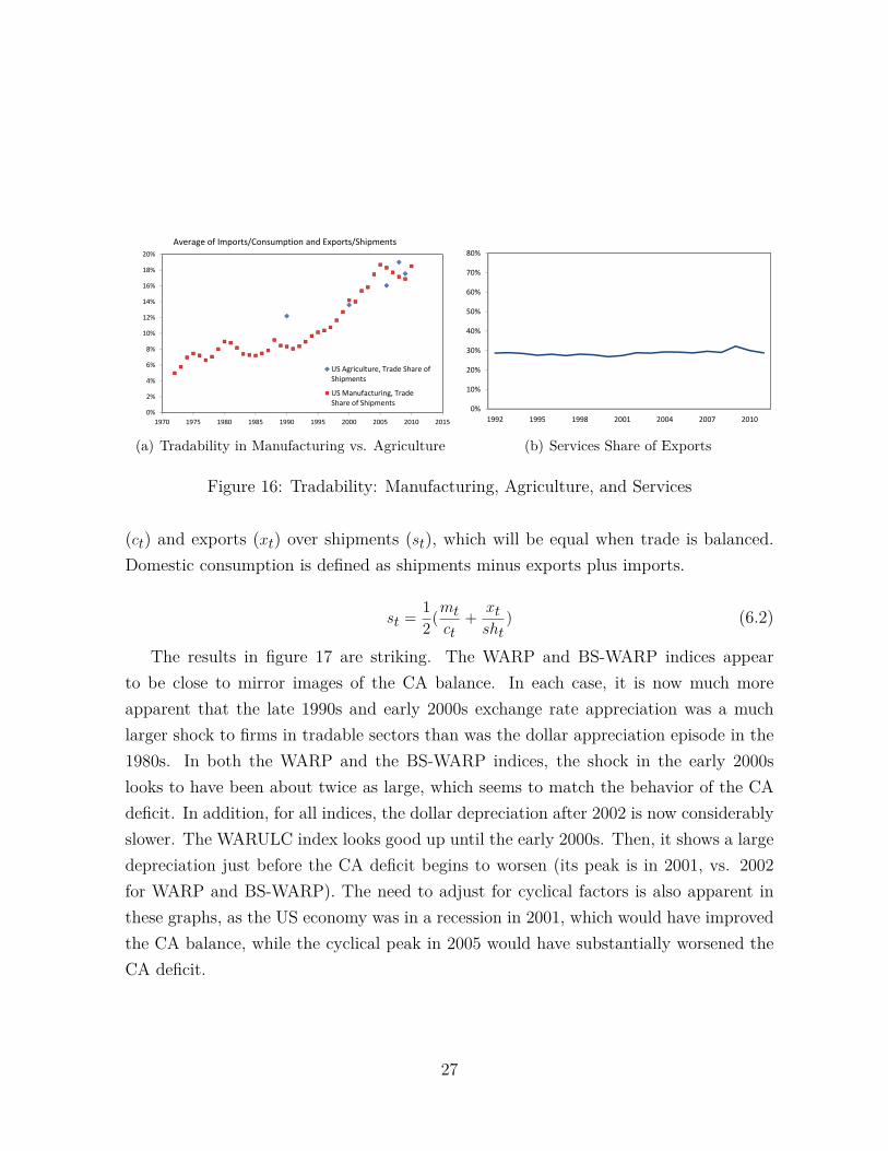
Ideal trade-weights would require information on domestic shipments and domesticconsumption for all trading partners, which is not readily available. A simple approxi-mation would be to assume that all exports compete primarily with foreign goods, andthat all domestic shipments compete with foreign competition based on the share ofimports in home consumption. The export share of shipments and the import share ofhome consumption in all tradables sectors can be proxied using manufacturing sectordata. Manufacturing accounts for a large share of US trade, having been 63% of totalUS trade in 1992, declining only slowly to about 60% by 2006, although it did declinesharply after 2007. Another large component of traded goods is agriculture, which Fig-ure 16(a) shows has tended to have a roughly similar share of traded goods in productionand consumption as manufacturing over the past several decades. This implies that us-ing data on manufacturing, which still accounts for a majority of US trade, as a proxyfor traded shares of tradable goods overall is reasonable. A third major category oftrade is services, which economists frequently stress has witnessed impressive growth intrade. However, contrary to many economists’ priors, the BEA data presented in Figure16(b) show that services exports as a share of total US exports have remained relativelyconstant over the past few decades.

Thus, in terms of the indices computed ignoring the role of domestic market compe-tition, an index adjusted for domestic competition could be written as:

Inewj,t = Ioldj,t ∗ st + 1 ∗ (1− st). (6.1)

Thus the modified index would simply be a weighted average of the real exchangerate index with trading partners time the trade share st plus the real exchange ratewith domestic competitors (one) times the share of domestic competition out of totalcompetitors. The trade share is an average of imports (mt) over domestic consumption

26

10%

12%

14%

16%

18%

20%

Average of Imports/Consumption and Exports/Shipments

0%

2%

4%

6%

8%

1970 1975 1980 1985 1990 1995 2000 2005 2010 2015

US Agriculture, Trade Share of

Shipments

US Manufacturing, Trade

Share of Shipments

(a) Tradability in Manufacturing vs. Agriculture

30%

40%

50%

60%

70%

80%

0%

10%

20%

30%

1992 1995 1998 2001 2004 2007 2010

(b) Services Share of Exports

Figure 16: Tradability: Manufacturing, Agriculture, and Services

(ct) and exports (xt) over shipments (st), which will be equal when trade is balanced.Domestic consumption is defined as shipments minus exports plus imports.

st = 12(mt

ct+ xtsht

) (6.2)

The results in figure 17 are striking. The WARP and BS-WARP indices appearto be close to mirror images of the CA balance. In each case, it is now much moreapparent that the late 1990s and early 2000s exchange rate appreciation was a muchlarger shock to firms in tradable sectors than was the dollar appreciation episode in the1980s. In both the WARP and the BS-WARP indices, the shock in the early 2000slooks to have been about twice as large, which seems to match the behavior of the CAdeficit. In addition, for all indices, the dollar depreciation after 2002 is now considerablyslower. The WARULC index looks good up until the early 2000s. Then, it shows a largedepreciation just before the CA deficit begins to worsen (its peak is in 2001, vs. 2002for WARP and BS-WARP). The need to adjust for cyclical factors is also apparent inthese graphs, as the US economy was in a recession in 2001, which would have improvedthe CA balance, while the cyclical peak in 2005 would have substantially worsened theCA deficit.

27

11.

051.

11.

15W

AR

P in

cl S

elf−

Com

petit

ion

.81

1.2

1.4

WA

RP

v8.

0

1970 1980 1990 2000 2010

WARP v8.0 WARP incl Self−Competition

(a) vs. WARP

11.

051.

11.

15W

AR

P in

cl S

elf−

Com

petit

ion

−6

−4

−2

0C

A B

alan

ce

1980 1990 2000 2010

CA Balance WARP incl Self−Competition

(b) vs. the US CA Balance.9

81

1.02

1.04

1.06

1.08

BS

−W

AR

P in

cl S

elf−

Com

petit

ion

.8.9

11.

11.

21.

3B

S−

WA

RP

1970 1980 1990 2000 2010

BS−WARP BS−WARP incl Self−Competition

(c) vs. BS-WARP

.98

11.

021.

041.

061.

08B

S−

WA

RP

incl

Sel

f−C

ompe

titio

n

−6

−4

−2

0C

A B

alan

ce

1980 1990 2000 2010

CA Balance BS−WARP incl Self−Competition

(d) vs. the US CA Balance

11.

051.

11.

15W

AR

ULC

incl

Sel

f−C

ompe

titio

n

11.

11.

21.

31.

41.

5W

AR

ULC

(m

ult.

benc

hmar

ks)

1970 1980 1990 2000 2010

WARULC (mult. benchmarks) WARULC incl Self−Competition

(e) vs. WARULC

11.

051.

11.

15W

AR

ULC

incl

Sel

f−C

ompe

titio

n

−6

−4

−2

0C

A B

alan

ce

1980 1990 2000 2010

CA Balance WARULC incl Self−Competition

(f) vs. the US CA Balance

Figure 17: Comparing Indices with Weights for Self-Competition

28

7 WARULC vs. IMF RULC: Empirical Tests

The main point of this paper is to introduce new and improved measures of relativeprices. Fahle et al. (2008) display that relative price indices based on WARP seems todo a better job predicting US trade imbalances than do divisia-based indices using CPIs.While it would be nice to extend this evidence using WARP for the period 1820 to 1970,most of the large movements in relative prices during this period were associated withmajor wars or the Great Depression, and so exchange rates were unlikely to be the majordeterminate of trade flows as they arguably were in the post-Bretton Woods period.Instead, in this section, we focus on our new relative unit labor cost index, presentingevidence that WARULC does a better job predicting aggregate manufacturing tradefor the US than does the IMF’s index, and also that it does a remarkably good jobpredicting the timing of the collapse of import-competing manufacturing sectors.

First, in Figure 18 we show that the level of WARULC seems to do a reasonably goodjob of predicting changes in the import share of manufacturing trade not due to changesin GDP.9 The IMF’s RULC index, by contrast, implies a steadily more competitive USmanufacturing sector over time, which seems to be at odds with the large import shareof trade the US has experienced since the late 1990s, and at odds with the realizedcollapse in US manufacturing in the early 2000s concentrated in sectors more-exposedto international trade (Campbell 2014) and Chinese import competition (Autor et al.2013).

Second, we postulate a simple model based on intuitive priors to predict the shareof manufactured imports of total manufacturing trade:

MUS,t = α + ρMUS,t−1 + β0ln∆RGDPOt + β1ln∆RGDPO∗t + β2Ijt−1 + εt, (7.1)

j = WARULC, IMF RULC Index.10

This equation supposes that the import share of manufacturing trade (MUS,t) growswhen home GDP growth is higher (RGDPOt), falls when foreign GDP growth is faster(RGDPO∗t ), and rises when the lagged level of the real exchange rate is higher (Ijt−1). Theresults are displayed in Table 1, which shows that each coefficient is of the theoretically

9I.e., they do a good job of explaining the residuals of regression: MUS,t = α + ρMUS,t−1 +β0ln∆RGDPOt + β1ln∆RGDPO∗t + β2I

jt−1 + εt, with the lagged value of WARULC times the co-

efficient on the lagged value of WARULC added back in.10We do not have enough observations in this case to do an error correction model. Note that we

start in 1975 because this is when the IMF’s index begins.

29

.81

1.2

1.4

1.6

.05

.1.1

5.2

Res

idua

ls: I

mpo

rt S

hare

of T

rade

1970 1980 1990 2000 2010

Residuals: Import Share of Trade WARULCIMF RULC

Figure 18: RULC Indices vs. Import Share of Manufacturing Trade

predicted sign. We find that the R-squared is higher using WARULC than it is using theIMF’s RULC index, and also more highly significant. This simple estimation strategybased on intuitive priors is not without trouble, as in the regression using the IMF’sindex, the coefficients on GDP and the lagged import share of trade likely change ina way that would be unlikely to hold out of sample, in order to counteract the strongnegative trend in the IMF’s index. An additional problem with using a lagged dependentvariable is Nickell (1981) bias, where the lagged dependent variable will be equal to(1+ρ)/(T-1), which should be on the order of 5% with t=33 in this case, which we argueis not material.

Campbell (2014) finds that the class of Weighted-Average Relative (WAR) price in-dices developed in this paper can predict declines in more open manufacturing sectorsrelative to less open manufacturing sectors, which, he argues, are less exposed to in-ternational trade. We confirm and strengthen this evidence, by showing (Figure 19)that our import-Weighted Average Relative Unit Labor Cost (iWARULC) index does aremarkably good job predicting years when manufacturing sectors with a higher shareof import-penetration suffered declines in employment. The coefficient on import pene-

30

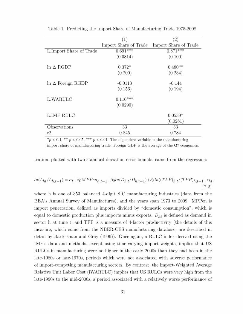
Table 1: Predicting the Import Share of Manufacturing Trade 1975-2008

(1) (2)Import Share of Trade Import Share of Trade

L.Import Share of Trade 0.691*** 0.871***(0.0814) (0.100)

ln ∆ RGDP 0.372* 0.480**(0.200) (0.234)

ln ∆ Foreign RGDP -0.0113 -0.144(0.156) (0.194)

L.WARULC 0.116***(0.0290)

L.IMF RULC 0.0539*(0.0281)

Observations 33 33r2 0.845 0.784*p < 0.1, ** p < 0.05, *** p < 0.01. The dependent variable is the manufacturingimport share of manufacturing trade. Foreign GDP is the average of the G7 economies.

tration, plotted with two standard deviation error bounds, came from the regression:

ln(Lht/Lh,t−1) = αt+β0MPPenh,t−1+β2ln(Dh,t/Dh,t−1)+β3ln((TFP )h,t/(TFP )h,t−1+εht,(7.2)

where h is one of 353 balanced 4-digit SIC manufacturing industries (data from theBEA’s Annual Survey of Manufactures), and the years span 1973 to 2009. MPPen isimport penetration, defined as imports divided by “domestic consumption”, which isequal to domestic production plus imports minus exports. Dht is defined as demand insector h at time t, and TFP is a measure of 4-factor productivity (the details of thismeasure, which come from the NBER-CES manufacturing database, are described indetail by Bartelsman and Gray (1996)). Once again, a RULC index derived using theIMF’s data and methods, except using time-varying import weights, implies that USRULCs in manufacturing were no higher in the early 2000s than they had been in thelate-1980s or late-1970s, periods which were not associated with adverse performanceof import-competing manufacturing sectors. By contrast, the import-Weighted AverageRelative Unit Labor Cost (iWARULC) implies that US RULCs were very high from thelate-1990s to the mid-2000s, a period associated with a relatively worse performance of

31

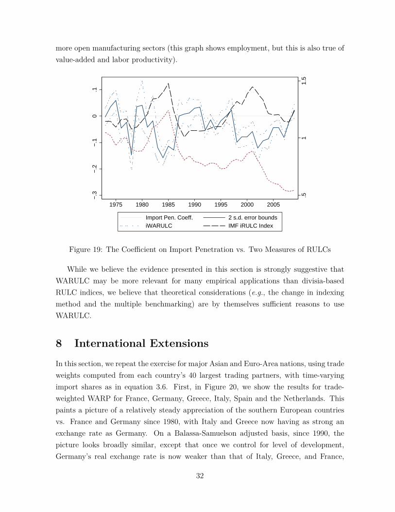
more open manufacturing sectors (this graph shows employment, but this is also true ofvalue-added and labor productivity).

.51

1.5

−.3

−.2

−.1

0.1

1975 1980 1985 1990 1995 2000 2005

Import Pen. Coeff. 2 s.d. error boundsiWARULC IMF iRULC Index

Figure 19: The Coefficient on Import Penetration vs. Two Measures of RULCs

While we believe the evidence presented in this section is strongly suggestive thatWARULC may be more relevant for many empirical applications than divisia-basedRULC indices, we believe that theoretical considerations (e.g., the change in indexingmethod and the multiple benchmarking) are by themselves sufficient reasons to useWARULC.

8 International Extensions

In this section, we repeat the exercise for major Asian and Euro-Area nations, using tradeweights computed from each country’s 40 largest trading partners, with time-varyingimport shares as in equation 3.6. First, in Figure 20, we show the results for trade-weighted WARP for France, Germany, Greece, Italy, Spain and the Netherlands. Thispaints a picture of a relatively steady appreciation of the southern European countriesvs. France and Germany since 1980, with Italy and Greece now having as strong anexchange rate as Germany. On a Balassa-Samuelson adjusted basis, since 1990, thepicture looks broadly similar, except that once we control for level of development,Germany’s real exchange rate is now weaker than that of Italy, Greece, and France,

32

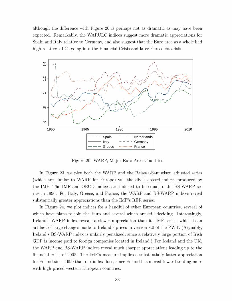
although the difference with Figure 20 is perhaps not as dramatic as may have beenexpected. Remarkably, the WARULC indices suggest more dramatic appreciations forSpain and Italy relative to Germany, and also suggest that the Euro area as a whole hadhigh relative ULCs going into the Financial Crisis and later Euro debt crisis.

.6.8

11.

21.

4

1950 1965 1980 1995 2010

Spain NetherlandsItaly GermanyGreece France

Figure 20: WARP, Major Euro Area Countries

In Figure 23, we plot both the WARP and the Balassa-Samuelson adjusted series(which are similar to WARP for Europe) vs. the divisia-based indices produced bythe IMF. The IMF and OECD indices are indexed to be equal to the BS-WARP se-ries in 1990. For Italy, Greece, and France, the WARP and BS-WARP indices revealsubstantially greater appreciations than the IMF’s RER series.

In Figure 24, we plot indices for a handful of other European countries, several ofwhich have plans to join the Euro and several which are still deciding. Interestingly,Ireland’s WARP index reveals a slower appreciation than its IMF series, which is anartifact of large changes made to Ireland’s prices in version 8.0 of the PWT. (Arguably,Ireland’s BS-WARP index is unfairly penalized, since a relatively large portion of IrishGDP is income paid to foreign companies located in Ireland.) For Iceland and the UK,the WARP and BS-WARP indices reveal much sharper appreciations leading up to thefinancial crisis of 2008. The IMF’s measure implies a substantially faster appreciationfor Poland since 1990 than our index does, since Poland has moved toward trading morewith high-priced western European countries.

33

.6.8

11.

21.

4

1970 1980 1990 2000 2010

Spain NetherlandsItaly GermanyGreece France

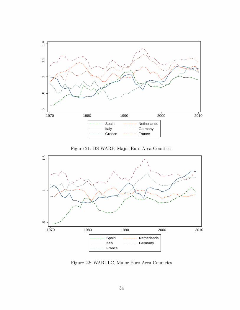
Figure 21: BS-WARP, Major Euro Area Countries

.51

1.5

1970 1980 1990 2000 2010

Spain NetherlandsItaly GermanyFrance

Figure 22: WARULC, Major Euro Area Countries

34

.85

.9.9

51

1.05

1.1

1990 1995 2000 2005 2010

Spain SpainIMF RER Index (set = to BS−WARP in 1990)

(a) Spain

.8.9

11.

11.

2

1990 1995 2000 2005 2010

Italy ItalyIMF RER Index (set = to BS−WARP in 1990)

(b) Italy

.7.8

.91

1.1

1990 1995 2000 2005 2010

Greece GreeceIMF RER Index (set = to BS−WARP in 1990)

(c) Greece

11.

11.

21.

31.

4

1990 1995 2000 2005 2010

Germany GermanyIMF RER Index (set = to BS−WARP in 1990)

(d) Germany

11.

11.

21.

3

1990 1995 2000 2005 2010

France FranceIMF RER Index (set = to BS−WARP in 1990)

(e) France

.91

1.1

1.2

1.3

1980 1990 2000 2010

Netherlands NetherlandsIMF RER Index (set = to BS−WARP in 1990)

(f) Netherlands

Figure 23: BS-WARP and WARP vs. IMF Divisia RER Index

35

.91

1.1

1.2

1980 1990 2000 2010

BS−WARP WARPIMF RER Index (set = to BS−WARP in 1990)

(a) Ireland

.51

1.5

2

1980 1990 2000 2010

BS−WARP WARPIMF RER Index (set = to BS−WARP in 1990)

(b) Iceland

.4.6

.81

1.2

1995 2000 2005 2010

BS−WARP WARPBIS RER Index (set = to BS−WARP in 1994)

(c) Latvia

.2.4

.6.8

1

1980 1990 2000 2010

BS−WARP WARPIMF RER Index (set = to BS−WARP in 1990)

(d) Romania

.81

1.2

1.4

1980 1990 2000 2010

BS−WARP WARPIMF RER Index (set = to BS−WARP in 1990)

(e) UK

.2.4

.6.8

11.

2

1990 1995 2000 2005 2010

BS−WARP WARPIMF RER Index (set = to BS−WARP in 1990)

(f) Poland

Figure 24: BS-WARP and WARP vs. IMF Divisia RER Index

36

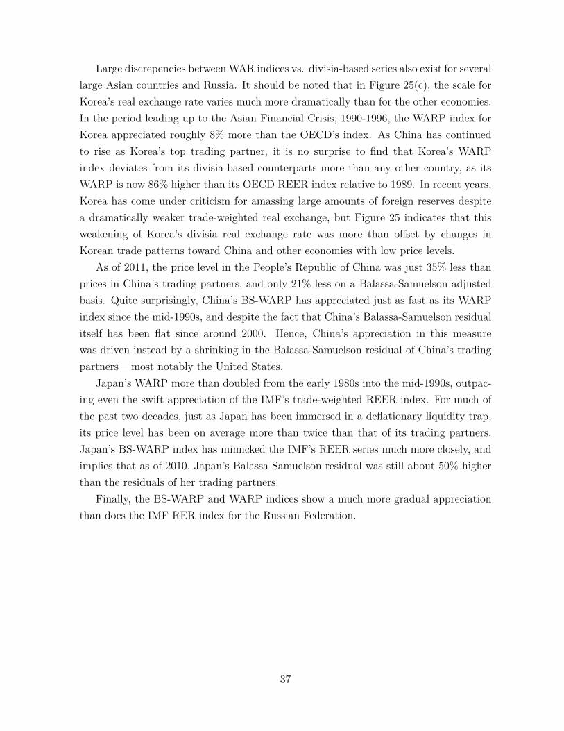
Large discrepencies betweenWAR indices vs. divisia-based series also exist for severallarge Asian countries and Russia. It should be noted that in Figure 25(c), the scale forKorea’s real exchange rate varies much more dramatically than for the other economies.In the period leading up to the Asian Financial Crisis, 1990-1996, the WARP index forKorea appreciated roughly 8% more than the OECD’s index. As China has continuedto rise as Korea’s top trading partner, it is no surprise to find that Korea’s WARPindex deviates from its divisia-based counterparts more than any other country, as itsWARP is now 86% higher than its OECD REER index relative to 1989. In recent years,Korea has come under criticism for amassing large amounts of foreign reserves despitea dramatically weaker trade-weighted real exchange, but Figure 25 indicates that thisweakening of Korea’s divisia real exchange rate was more than offset by changes inKorean trade patterns toward China and other economies with low price levels.

As of 2011, the price level in the People’s Republic of China was just 35% less thanprices in China’s trading partners, and only 21% less on a Balassa-Samuelson adjustedbasis. Quite surprisingly, China’s BS-WARP has appreciated just as fast as its WARPindex since the mid-1990s, and despite the fact that China’s Balassa-Samuelson residualitself has been flat since around 2000. Hence, China’s appreciation in this measurewas driven instead by a shrinking in the Balassa-Samuelson residual of China’s tradingpartners – most notably the United States.

Japan’s WARP more than doubled from the early 1980s into the mid-1990s, outpac-ing even the swift appreciation of the IMF’s trade-weighted REER index. For much ofthe past two decades, just as Japan has been immersed in a deflationary liquidity trap,its price level has been on average more than twice than that of its trading partners.Japan’s BS-WARP index has mimicked the IMF’s REER series much more closely, andimplies that as of 2010, Japan’s Balassa-Samuelson residual was still about 50% higherthan the residuals of her trading partners.

Finally, the BS-WARP and WARP indices show a much more gradual appreciationthan does the IMF RER index for the Russian Federation.

37

.2.4

.6.8

1

1980 1990 2000 2010

BS−WARP WARPIMF RER Index (set = to BS−WARP in 1990)

(a) People’s Republic of China

11.

52

2.5

1970 1980 1990 2000 2010

BS−WARP WARPIMF RER Index (set = to BS−WARP in 1990)

(b) Japan

.4.6

.81

1.2

1980 1990 2000 2010

BS−WARP WARPKorea OECD REER Index

(c) Korea

.2.4

.6.8

1

1990 1995 2000 2005 2010

BS−WARP WARPIMF RER Index (set = to BS−WARP in 1994)

(d) Russian Federation

Figure 25: BS-WARP and WARP vs. IMF Divisia RER Index

38

9 Conclusion

In this paper, we sought to improve the methodology used to create trade-weightedreal exchange rate indices, proposing several new series, including a Balassa-Samuelsonadjusted Weighted Average Relative Price index, and a Weighted Average Relative UnitLabor Cost index, which are designed to solve the trading partner substitution biasproblem and control for productivity as per the Penn Effect. Our new indices providea seriously warped view of recent economic history, both in the US and internationally.We demonstrate that, for many countries currently mired in liquidity traps, includingJapan, the US, and for the Euro area, prices and wages had grown to high levels relativeto trading partners heading into the financial crisis of 2008. For the US, we demonstratethat in 2002 – during the surprisingly swift collapse of US manufacturing – relative priceshad not been that high since the worst year of the Great Depression, when the goldenstraitjacket led to an appreciated currency, collapsing commodity prices, rising real debtlevels and a financial and economic crisis. We believe anyone wishing to understand thepast 20 years of economic history would do well to start with relative prices.

References

Allen, R. C., J.-P. Bassino, D. Ma, C. Moll-Murata and J. L. Van Zanden,“Wages, Prices, and Living Standards in China, 1738–1925: In Comparison withEurope, Japan, and India,” The Economic History Review 64 (2011), 8–38.

Autor, D., D. Dorn and G. H. Hanson, “The China Syndrome: The Local LaborMarket Effects of Import Competition in the US,” American Economic Review 103(2013), 2121–68.

Bai, C.-E. and Z. Qian, “The Factor Income Distribution in China: 1978–2007,”China Economic Review 21 (2010), 650–670.

Bai, R. R., Manyin and A. Szirmai, “Chinese Manufacturing Performance in Com-parative Perspective, 1980-2002,” Yale University Economic Growth Center Discus-sion Paper (2005).

Barbieri, K., The Liberal Illusion: Does Trade Promote Peace? (University of Michi-gan Press, 2002).

Bartlesman, E. and W. B. Gray, “The NBER Manufacturing ProductivityDatabase,” (1996).

39

Bayoumi, T., M. Saito and J. Turunen, “Measuring Competitiveness: Trade inGoods or Tasks?,” (2013).

Bayoumi, T. A., J. Lee, S. Jayanthi and G. M. Milesi-Ferretti, New RatesFrom New Weights, 5860 (International Monetary Fund, 2005).

Bems, R. and R. C. Johnson, “Value-Added Exchange Rates,” Working Paper 18498,National Bureau of Economic Research, October 2012.

Bergin, P. R., R. Glick and A. M. Taylor, “Productivity, Tradability, and theLong-Run Price Puzzle,” Journal of Monetary Economics 53 (2006), 2041–2066.

Campbell, D. L., “Relative Prices, Hysteresis, and the Decline of American Manufac-turing,” (2014).

Catao, L. and S. Solomou, “Effective exchange rates 1879–1913,” European Reviewof Economic History 4 (2000), 361–382.

Ceglowski, J. and S. S. Golub, “Does China Still Have a Labor Cost Advantage?,”Global Economy Journal 12 (2012).

Chinn, M. D., “Before the Fall: Were East Asian Currencies Overvalued?,” EmergingMarkets Review 1 (2000), 101–126.

———, “Incomes, Exchange Rates and the US Trade Deficit, Once Again*,” Interna-tional Finance 7 (2004), 451–469.

Desruelle, D. and A. Zanello, “A Primer on the IMFs Information Notice System,”IMF Working Paper No. 97/71 (1997).

Devereux, J. and M. Ward, “Measuring British Decline: Direct Versus Long-spanIncome Measures,” The Journal of Economic History 63 (2003), 826–851.

———, “Relative British and American Income Levels During the First Industrial Rev-olution,” Research in Economic History 23 (2006), 249–286.

Diewert, W. E., A. O. Nakamura, J. S. Greenlees, L. I. Nakamura andM. B. Reinsdorf, “Sourcing Substitution and Related Price Index Biases,” (2014).

Fahle, S., J. Marquez and C. Thomas, “Measuring US International RelativePrices: A WARP View of the World,” FRB International Finance Discussion Paper(2008).

40

———, “Measures of International Relative Prices for China and the USA,” PacificEconomic Review 14 (2009), 376–397.

Feenstra, R. C., R. Inklaar and M. Timmer, “The Next Generation of the PennWorld Table,” (2011).

Feenstra, R. C., R. E. Lipsey, H. Deng, A. C. Ma and H. Mo, “World TradeFlows: 1962-2000,” Technical Report, National Bureau of Economic Research, 2005.

Feenstra, R. C., H. Ma, J. Peter Neary and D. Prasada Rao, “Who ShrunkChina? Puzzles in the Measurement of Real GDP,” The Economic Journal (2012).

Fratzscher, M., A. Mehl and I. Vansteenkiste, “130 Years of Fiscal Deficitsand Currency Crashes in Advanced Economies,” (2011).

Golub, S. and J. Ceglowski, “Just How Low are China’s Labour Costs?,” TheWorld Economy 30 (2007), 597–617.

———, “Does China Still Have a Labor Cost Advantage?,” (2011).

Golub, S. S. and A. G. Turner, “Towards a System of Multilateral Unit Labor Cost-Based Competitiveness Indicators for Advanced, Developing, and Transition Coun-tries,” Technical Report, International Monetary Fund, 1997.

Ho, L. S., “Globalization, Exports, and Effective Exchange Rate Indices,” Journal ofInternational Money and Finance 31 (2012), 996–1007.

Houseman, S., C. Kurz, P. Lengermann and B. Mandel, “Offshoring Bias inU.S. Manufacturing,” Journal of Economic Perspectives 25 (Spring 2011), 111–32.

Inklaar, R., “Offshoring Bias in Manufacturing Growth Across Advanced and Emerg-ing Economies,” (2012).

Irwin, D. A., “Trade Restrictiveness and Deadweight Loses from US Tariffs, 1859-1961,” Technical Report, National Bureau of Economic Research, 2007.

Jacks, D., C. Meissner and D. Novy, “Trade Booms, Trade Busts, and TradeCosts,” Journal of International Economics (2006).

Johnson, S., J. D. Ostry and A. Subramanian, “Prospects for Sustained Growthin Africa: Benchmarking the Constraints.,” IMF Staff Papers 57 (2010).

41

Loretan, M., “Indexes of the Foreign Exchange Value of the Dollar,” Fed. Res. Bull.91 (2005), 1.

Nickell, S., “Biases in dynamic models with fixed effects,” Econometrica: Journal ofthe Econometric Society (1981), 1417–1426.

Rodrik, D., “The Real Exchange Rate and Economic Growth,” Brookings Papers onEconomic Activity 2008 (2008), 365–412.

Schmitz, M., M. De Clercq, M. Fidora, B. Lauro and C. Pinheiro, “Revistingthe Effective Exchange Rates of the Euro,” ECB Occasional Paper (2011).

Skidelsky, R., John Maynard Keynes: Volume 2: The Economist as Savior, 1920-1937, volume 2 (Penguin Books, 1995).

Taylor, A. M., “A Century of Purchasing-Power Parity,” Review of Economics andStatistics 84 (2002), 139–150.

Turner, P. and J. Van’t Dack, “Measuring International Price and Cost Compet-itiveness,” Bank for International Settlements, Monetary and Economic Department(1993).

42

10 Appendix

Year

Ward and

Devereux

Our

Estimates Allen et al .

Our

Estimates

1831 156 143.9

1839 122 134.6

1849 123 133.6

1859 112 124.7

1869 110 105.6

1872 108 105.8

1874 113 112.5

1878 112 110.3

1884* 94 106.6 200.5 194.2

1891* 99 113.0 147.3 147.3

1905 83 121.2 121.5 112.7

1930 83 95.5

1950 71 56.4

1955 82 64.5

1967 83 75.9

1970 72 67.2

1973 84 76.4

*For Japan, the comparisons are for 1886 and 1892.

UK Japan

Table A.1: Historical Relative Price Levels (vs. US)

43

Table A.2: Historical US vs. Federal Reserve Samples

Country Historical Sample Start Post-war Sample Start

1. China 1820 19502. Netherlands 1820 19503. Norway 1820 19504. Spain 1820 19505. Sweden 1820 19506. UK 1820 19507. Belgium 1830 19508. Brazil 1830 19509. France 1840 195010. Germany 1852 195011. Australia 1861 195012. Italy 1861 195013. Denmark 186414. Japan 1868 195015. India 1873 195016. Chile 1880 195017. Austria 1884 195018. Switzerland 1885 195019. Uruguay 188520. Egypt 189521. South Africa 189522. Peru 190023. Venezuela 1900 195024. Philippines 1902 195025. Canada 1910 195026. New Zealand 191427. Colombia 1919 195028. Finland 1920 195029. Greece 1922 200130. Turkey 192231. Hong Kong 195032. South Korea 195033. Singapore 195034. Russia 199335. Taiwan 195036. Malaysia 195037. Mexico 195038. Euro Area 199939. Israel 195040. Indonesia 195041. Saudi Arabia 1950

44

Data Source URL

Bilateral Trade Data (total flows) IMF Dots http://elibrary-data.imf.org/

Bilateral Trade in Oil UN Comtrade http://comtrade.un.org/

Federal Reserve Trade Weights Federal Reserve Board of Governors http://www.federalreserve.gov/releases/h10/weights/

Fed's Broad Trade-Weighted Real Exchange

Rate, Korean Inflation Federal Reserve Economic Data http://research.stlouisfed.org/fred2/

PPP, Real GDP, Exchange Rates Penn World Tables, v7.1 and v8.0 http://www.rug.nl/research/ggdc/data/penn-world-table

Historical Exchange Rates Bordo https://sites.google.com/site/michaelbordo/home4

Historical Inflation, Trade Data Historical Statistics of the United States http://hsus.cambridge.org/

Historical Trade Data Barbieri (2002) http://people.cas.sc.edu/barbierk/databases.html

Historical Trade and Tariff Data Jacks, Meissner, Novy (2009) N/A

World Bank http://econ.worldbank.org

Historical Tariff Data Irwin (2007) http://www.nber.org/papers/w13450

Post-war Taiwan Inflation Taiwanese Government http://eng.stat.gov.tw/mp.asp?mp=5

Post-War Tariff Data UN Comtrade http://comtrade.un.org/

Manufacturing Data (Employment, etc.) BEA, Annual Survey of Manufactures www.census.gov/manufacturing/asm

Historical Exchange Rates Historical Volumes of Mitchell N/A

Historical Exchange Rates Wahrungen der Welt , Vol. 1-10 N/A

Historical Price Indices

Lindert & Arroyo Abad, Global Price and

Income History Group gpih.ucdavis.edu

British Prices From 1750 Office for National Statistics (ONS) http://www.ons.gov.uk

Chinese Historical Prices Allen et al. (2011) via gpih.ucdavis.edu

IMF Trade Weights Bayoumi et al . (2006) http://www.imf.org/external/pubs/ft/wp/wp9771.pdf

Tariff Data, 1984-1995 UNCTAD -- TRAINS www.unctad.info/en

Trade Data by SITC4, 1962-2008 Feenstra, Lipsey et al. 2005 cid.econ.ucdavis.edu

Manufacturing Labor Costs, Productivity UNIDOs INDSTAT http://data.un.org/

Manufacturing Labor Costs, Productivity BLS http://www.bls.gov/fls/

Relative Price Levels in Manufacturing

World Bank, International Comparison

Project 2005http://databank.worldbank.org/data/databases.aspx

Relative Price Levels in Manufacturing

Groningen Growth and Development

Centre Productivity Level Databasehttp://www.rug.nl/research/ggdc/data/

Manufacturing Labor Costs, Productivity, Trade OECD http://stats.oecd.org/

Canada, Manufacturing Deflator Statistics Canada http://www.statcan.gc.ca

Table A.3

Data Sources

Average MFN Applied Tariff Rates in

Developing and Industrial Countries

45