Embed Size (px)
Citation preview
Time Dependent VirtualMachine Consolidation withSLA (Service LevelAgreement) considerationYadassa H. AllaMaster’s Thesis Spring 2015

Contents
1 Introduction 31.1 Motivation . . . . . . . . . . . . . . . . . . . . . . . . . . . . . 31.2 Overview . . . . . . . . . . . . . . . . . . . . . . . . . . . . . . 31.3 Problem statement . . . . . . . . . . . . . . . . . . . . . . . . 51.4 Challenges of VM consolidation . . . . . . . . . . . . . . . . . 51.5 Approach . . . . . . . . . . . . . . . . . . . . . . . . . . . . . . 61.6 The goal of the thesis . . . . . . . . . . . . . . . . . . . . . . . 61.7 The structure of the thesis . . . . . . . . . . . . . . . . . . . . 7
2 Background 92.1 Background . . . . . . . . . . . . . . . . . . . . . . . . . . . . 9
2.1.1 Cloud computing . . . . . . . . . . . . . . . . . . . . . 92.1.2 Virtualization . . . . . . . . . . . . . . . . . . . . . . . 112.1.3 Hypervisor . . . . . . . . . . . . . . . . . . . . . . . . 122.1.4 Virtual Machines . . . . . . . . . . . . . . . . . . . . . 132.1.5 Virtual Machine (VM) Consolidation . . . . . . . . . . 132.1.6 Bin Packing . . . . . . . . . . . . . . . . . . . . . . . . 162.1.7 Service Level Agreement . . . . . . . . . . . . . . . . 17
2.2 Auto-Scaling Techniques . . . . . . . . . . . . . . . . . . . . . 172.2.1 CPU Consumption and Power Relationship . . . . . 182.2.2 Dynamic Voltage and Frequency Scaling . . . . . . . 18
2.3 Data Center . . . . . . . . . . . . . . . . . . . . . . . . . . . . 182.4 Cloud Data Center . . . . . . . . . . . . . . . . . . . . . . . . 182.5 Covariance . . . . . . . . . . . . . . . . . . . . . . . . . . . . . 192.6 Correlation . . . . . . . . . . . . . . . . . . . . . . . . . . . . . 192.7 Related works . . . . . . . . . . . . . . . . . . . . . . . . . . . 20
3 Methodology 233.1 Objective of the experiment . . . . . . . . . . . . . . . . . . . 233.2 System Architecture . . . . . . . . . . . . . . . . . . . . . . . . 24
3.2.1 Description of the System architecture . . . . . . . . . 243.2.2 Assumptions . . . . . . . . . . . . . . . . . . . . . . . 243.2.3 Tools . . . . . . . . . . . . . . . . . . . . . . . . . . . . 25
3.3 Data . . . . . . . . . . . . . . . . . . . . . . . . . . . . . . . . . 253.3.1 Characteristics of the Data-set . . . . . . . . . . . . . . 26
3.4 Experimental Setup . . . . . . . . . . . . . . . . . . . . . . . . 273.4.1 Approaches for VM Consolidation . . . . . . . . . . 27
i
CONTENTS CONTENTS
3.5 Policies for SLA . . . . . . . . . . . . . . . . . . . . . . . . . . 33
4 Results 374.1 Evaluation Metrics . . . . . . . . . . . . . . . . . . . . . . . . 374.2 Number of utilized PMs . . . . . . . . . . . . . . . . . . . . . 38
4.2.1 Number of VMs on each PM . . . . . . . . . . . . . . 384.2.2 Diterministic Approach VM Location . . . . . . . . . 394.2.3 Stochastic approach I VM location . . . . . . . . . . . 394.2.4 Stochastic Approach II VM location . . . . . . . . . . 40
4.3 Total number of SLA Violations . . . . . . . . . . . . . . . . . 404.4 Description of Results . . . . . . . . . . . . . . . . . . . . . . 42
4.4.1 Observation on PMs utilization . . . . . . . . . . . . . 424.4.2 Observation on SLA violation . . . . . . . . . . . . . . 43
4.5 Evaluation Days Result . . . . . . . . . . . . . . . . . . . . . . 454.5.1 Number of utilized PMs . . . . . . . . . . . . . . . . . 454.5.2 Total number of SLA violations . . . . . . . . . . . . . 45
4.6 Description of Evaluation Days Result . . . . . . . . . . . . . 474.6.1 Observation on PM utilization . . . . . . . . . . . . . 474.6.2 Observation on SLA violation . . . . . . . . . . . . . . 47
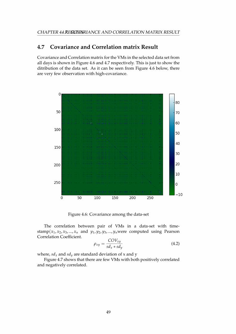
4.7 Covariance and Correlation matrix Result . . . . . . . . . . . 49
5 Discussion 535.1 Summary . . . . . . . . . . . . . . . . . . . . . . . . . . . . . . 55
6 Conclusion and Future work 57
Appendices 61.1 Appendix A: Main Script . . . . . . . . . . . . . . . . . . . . . 61.2 Appendix B: Bin Packing Script for Deterministic approach
script . . . . . . . . . . . . . . . . . . . . . . . . . . . . . . . . 66.3 Appendix C: Stochastic I approach bin packing script . . . . 67.4 Appendix D: Stochastic Approach II bin packing Script . . . 69.5 Appendix E: SLA Violatioin Counter and grapher . . . . . . 71.6 Appendix F: Miscellaneous Figures . . . . . . . . . . . . . . . 73
.6.1 Number of VMs on each PM . . . . . . . . . . . . . . 73
.6.2 Stochastic approach I VM location . . . . . . . . . . . 73
.6.3 Stochastic approach II VM location . . . . . . . . . . 76
ii
List of Figures
2.1 Service Layer . . . . . . . . . . . . . . . . . . . . . . . . . . . 102.2 Virtualization Layer . . . . . . . . . . . . . . . . . . . . . . . . 122.3 Type I and Type II hypervisors . . . . . . . . . . . . . . . . . 132.4 Live Migration of VMs . . . . . . . . . . . . . . . . . . . . . . 152.5 Bin Packing:First Fit Decreasing when large items are packed
first . . . . . . . . . . . . . . . . . . . . . . . . . . . . . . . . . 17
3.1 Architecture of the System Model . . . . . . . . . . . . . . . . 24
4.1 Number of VMs on each physical machine with capacity 120 394.2 Number of VMs on each physical machine with capacity 120
and α = 0.05 . . . . . . . . . . . . . . . . . . . . . . . . . . . . 394.3 Number of VMs on each physical machine with capacity 120
and α = 0.05 . . . . . . . . . . . . . . . . . . . . . . . . . . . . 404.4 Total SLA violation for Day1 to Day8 . . . . . . . . . . . . . . 444.5 Total SLA violation for Day9 and Day10 . . . . . . . . . . . . 484.6 Covariance among the data-set . . . . . . . . . . . . . . . . . 494.7 Correlation among the data-set . . . . . . . . . . . . . . . . . 50
.61 Number of VMs on each physical machine with capacity 140 73
.62 Number of VMs on each physical machine with capacity 120and α = 0.5 . . . . . . . . . . . . . . . . . . . . . . . . . . . . . 73
.63 Number of VMs on each physical machine with capacity 120and α = 0.95 . . . . . . . . . . . . . . . . . . . . . . . . . . . . 74
.64 Number of VMs on each physical machine with capacity 140and α = 0.05 . . . . . . . . . . . . . . . . . . . . . . . . . . . . 74
.65 Number of VMs on each physical machine with capacity 140and α = 0.5 . . . . . . . . . . . . . . . . . . . . . . . . . . . . . 75
.66 Number of VMs on each physical machine with capacity 140and α = 0.95 . . . . . . . . . . . . . . . . . . . . . . . . . . . . 75
.67 Number of VMs on each physical machine with capacity 120and α = 0.5 . . . . . . . . . . . . . . . . . . . . . . . . . . . . . 76
.68 Number of VMs on each physical machine with capacity 120and α = 0.95 . . . . . . . . . . . . . . . . . . . . . . . . . . . . 76
.69 Number of VMs on each physical machine with capacity 140and α = 0.05 . . . . . . . . . . . . . . . . . . . . . . . . . . . . 77
.610 Number of VMs on each physical machine with capacity 140and α = 0.5 . . . . . . . . . . . . . . . . . . . . . . . . . . . . . 77
iii
LIST OF FIGURES LIST OF FIGURES
.611 Number of VMs on each physical machine with capacity 140and α = 0.95 . . . . . . . . . . . . . . . . . . . . . . . . . . . . 78
iv
List of Tables
3.1 PlanetLab workload-traces collected in March and April 2011 263.2 Table showing how mean of a VM is calculated . . . . . . . . 28
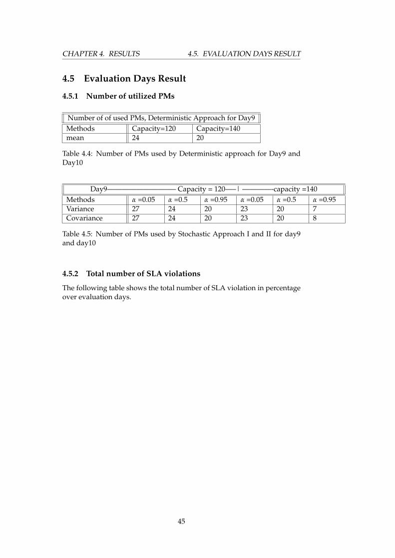
4.1 Number of PMs used, Out put from Deterministic approach 384.2 Number of PMs used by Stochastic Approach I and II . . . . 384.3 Total Number of SLA Violations in percentage . . . . . . . . 414.4 Number of PMs used by Deterministic approach for Day9
and Day10 . . . . . . . . . . . . . . . . . . . . . . . . . . . . . 454.5 Number of PMs used by Stochastic Approach I and II for
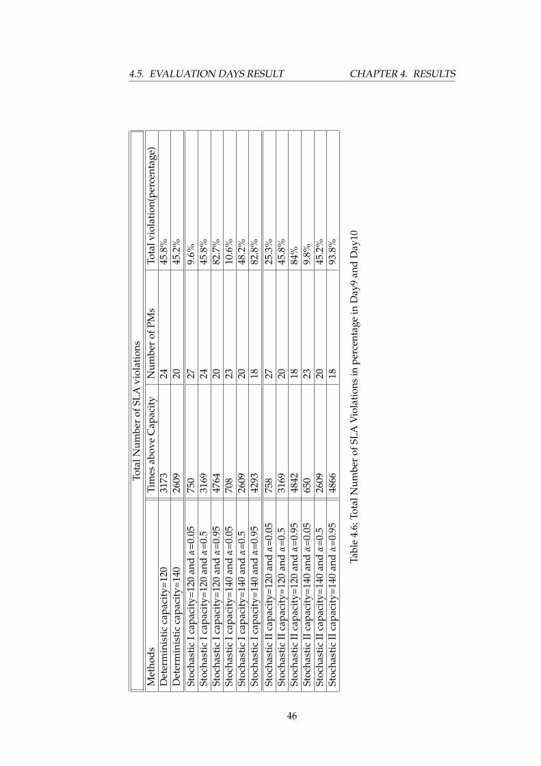
day9 and day10 . . . . . . . . . . . . . . . . . . . . . . . . . . 454.6 Total Number of SLA Violations in percentage in Day9 and
Day10 . . . . . . . . . . . . . . . . . . . . . . . . . . . . . . . . 46
5.1 Total Number of SLA Violations after introduction of 90% ofcapacity . . . . . . . . . . . . . . . . . . . . . . . . . . . . . . . 54
v

LIST OF TABLES LIST OF TABLES
vi
Acronyms
VM/s: Virtual Machine/sPM/s: Physical Machine/sSLA: Service Level AgreementQOS: Quality of ServiceCPU:Centeral Processor UnitCC:Cloud ComputingFFD: First Fit Decreasing
vii

LIST OF TABLES LIST OF TABLES
viii
Acknowledgement
Above all, I would like to acknowledge God for all the supports behind allwalks of my life.
Next,my special thanks goes to Oslo University informatics departmentAdministration staffs for allowing me to study this masters program.Furthermore, I would like to thank Oslo and Akershus University college,computer engineering department lecturers, who meant a lot for thesuccess. I owe thanks and respect for my supervisors Hugo Lewi Hammer(A.Professor at HioA) and Anis Yazidi(A.Professor at HioA) for theirunreserved advises and supports on my work. My special gratitude willbe for Hugo for his close follow up and guidance, patience and promptwhen ever I am in need of help.
All my class mates deserve thanks for their companion. It makes myday when I read their posts on facebook. Specially, my appreciation goesto Diako Kezri for being a good friend during this two years.
Lastly, I am more than words thank-full to my families (my wifeMarge, my daughter Kolu, my brother Jeto and his family)for their specialattachment and upholding my psychology during my studies. Withoutthem it wouldn’t be possible to wind up these two years. My lovely mom,Amasu Disasa, deserves uncountable love, thanks, respect, gratitude andall special due for her daily prayers which means a lot for my life.
ix

LIST OF TABLES LIST OF TABLES
x
Abstract
Cloud data center is becoming the most essential infrastructure for computing ser-vices. In effect, the operational cost of a data center is also increasing drastically.To decrease this cost, consolidation of VMs with less degradation of performance isso important. To guarantee the expected Quality of Service (QOS) the importantfactors to be controlled are performance of the service including timely leverageand overall resource utilization of the data center. In this paper, we tried to in-vestigate how to efficiently utilize resources with reduced SLA violation in a datacenter. In order to optimize efficiency, VMs ought to be consolidated as tight aspossible. To achieve this, an algorithm based on first fit decreasing (FFD) bin pack-ing is designed and implemented. Hence, the algorithm is implemented on thefollowing three approaches to pursue the goal: a)Deterministic Approach, whichis mainly based on mean of the individual VMs;b)Stochastic Approach I, whichis basically done by treating individual VMs based on their mean and variancesand ;c) Stochastic Approach II, which depends on mean and covariance of indi-vidual VMs. The results obtained show that consolidating VMs based on mean andvariance(stochastic approach I) performed better than the other two approaches forminimizing total percentage of SLA violation and stochastic approach II performedbetter than the two approaches for minimizing the number of PMs in consolidation.
xi

LIST OF TABLES LIST OF TABLES
1

LIST OF TABLES LIST OF TABLES
2
Chapter 1
Introduction
1.1 Motivation
Cloud Computing (CC) has drastically changed information technology(IT) since its emergence. The operating cost of Cloud data centers inthe world is also increasing significantly as the technology advances. Asdescribed by Jonathan G Koomey [22], it is assumed that electricity usedby data centers worldwide increased by about 56% from 2005 to 2010. In2010, it was accounted to be between 1.1% and 1.5% of total electricityuse respectively in the world. According to Natural Resource DefenceCouncil (NRDC) study, in 2013, electric consumption of data centers in USwas estimated to be 91 billion KW-hours, and projected to be 140 billionKW-hours in 2020. This costs 13 billion dollar annual expense for datacenters and 100 million metric tones of carbon emission annually[16]. Inthe increasing world of data center operational costs, system administratorcan play a significant role. Hence, it is duty of system administrators to findways to reduce the overall operational cost of the data centers and optimizethe resource utilization.
1.2 Overview
The rapid increase in Cloud Computing and IT end user focus hasdriven a big increase in Cloud data center importance. Because of this,data center administrators make constant effort to find ways to improveperformance, enhance infrastructure density, and increase multi-tenancycapabilities. As more converged systems make their way into the datacenter, infrastructure optimization will be critical to maintain a high levelof service[20]. Virtualization is one of the many ways of optimizing a datacenter.
In virtualization, Virtual machines (here after VM/VMs) are themost important components (resources). They depend on some otherphysical machine (Servers)or host to share resources such as CPU,memory,bandwidth and so on. These resources are consumed differentlyby each VM. Hence, it is customary to be interested in the relationshipbetween the VMs based on their consumption of the physical machine´s
3
1.2. OVERVIEW CHAPTER 1. INTRODUCTION
(host´s) resources, still relationship between them can also be studied us-ing different methodologies. Correlating peaks and valleys of the resourceconsumption is one of them. Besides, applications running on each VM dif-fer from one another, but still based on the communication between VMs,one can reach to a conclusion about the kind of relationship they have. Suchrelationships between VMs are discussed in detail by Xiaodong et al [34].
Studying the relationships among VMs helps to consolidate the VMs ina manner that can save resource utilization. One of the recommendationsthat the authors of [16] proposed to mitigate the power consumptionproblem of the data centers is to adopt server utilization metrics, likeaverage utilization of the Central Processing Unit (CPU) to adjust theconsumption if it surpasses a certain level. Reduction in resourceutilization and energy consumption can be achieved by dynamicallyconsolidating VMs and applying live migration, transferring VMs betweenphysical servers with minimum downtime and the likes.
In Cloud Computing, one of the main goal of consolidating VMs is toefficiently save the resource utilization and maintain the SLA (Service levelAgreement) for users as much as possible [12][2][29]. Degradation in QOS(Quality of service) from the side of service provider means violation ofSLA, thus Cloud service providers always strive to meet the SLA they havewith customers. As a result, Cloud service providers allow extra resourceto maintain SLA. Hence, resulting in the server sprawl, over-provisioningof resources than the requirement of the workload. Similarly, consumersmay also not use the resources they pay for due to reasonable factors. Thisresults in wastage of resource by letting them idle. It is estimated thatthe average server utilization in many data centers is between 10% and15%[24]. This is wasteful because an idle server often consumes about70% of its peak power, implying that servers at low utilization consumesignificantly more energy than some servers at high utilization. Thus, toprevent such wastage, it is advisable to consolidate them on fewer servers.Consolidation may result in cut for power consumption while degradingperformance, which results in SLA violation. The important concepts:Over-provisioning,allocating more resources than required to meet SLAand under-provisioning,allocating less resource than required to save theconsumption cost, are the other constant trade-offs in Cloud Computingenvironment. Live migration,migrating VMs if their resource consumptionsurpasses the capacity of resource supply of their host, helps to mitigatethese two concepts.
The trade-off that arises between performance and power-cost inconsolidating VMs is the crucial point in today’s data-centers[2]. Sincepower consumption goes linearly with number of physical machines, it isimportant to focus on minimizing the number of physical machines. Thus,this thesis contributes and proposes a solution for efficiently consolidatingVMs having in mind reduction in overall operational cost of a data center.In addition reducing SLA violation will be considered as additional focusso that performance will not be shaken.
4
CHAPTER 1. INTRODUCTION 1.3. PROBLEM STATEMENT
1.3 Problem statement
How to reduce operational cost of a data center by optimizing VM consolidationthat reduces resource consumption and minimize violation of SLA by taking ad-vantages of the dependence in usage patterns between VMs
Resource consumption in the problem statement is mainly relatedto consumption of physical machines. Reduction of physical machinesin effect reduces electric consumption. Data center’s consumption ofelectricity is increasing as technology grows. Therefore, the main goalof this thesis is to explore how to reduce the consumption of physicalmachines and as result reduce electricity consumption in a data center.
Optimizing refers to a technique that helps to achieve the mostadvantageous outcome in consolidating VMs. In this thesis, it is directlyattached to the algorithm that helps in packing (consolidating) the VMs into less number of physical machines and help efficiently utilize resources.
Dependence in Usage pattern refers to the way VMs are matched to beconsolidated. VM with high load will depend on VM with low load to saveresource consumption.
VM consolidation in the problem statement refers to packing togetherVMs based on their CPU utilization. Though there are many ways toconsolidate VMs three methodologies are preferred.These are:- a)based onthe mean CPU consumption of the individual VMs; b)based on mean andvariance in CPU consumption of individual VMs; c) based on mean andcovariance in CPU consumption of individual VMs.
SLA (Service Level Agreement) refers to the agreement between con-sumer or user and service provider to maintain agreed up on QOS (Qualityof service). It is basically setting threshold for consolidating VMs. If forexample the aggregate CPU utilization of VMs exceeds the capacity of thephysical machine then migrating the VM to another physical machine andor take another action. Generally, SLA violation happens when the aggreg-ate demand for the CPU performance of VMs surpasses the available CPUcapacity of a physical machine (hosting server).
1.4 Challenges of VM consolidation
Several studies [1][13] have shown that the basic challenges for efficientand dynamic VM consolidation are as follows:
• Host underload detection: Deciding if a host is considered to beunderloaded so that all VMs should be migrated from it and the hostshould be switched to a low-power mode (to minimize the numberof active physical servers).
• Host overload detection: Deciding if a host is considered to beoverloaded so that some VMs should be migrated from it to otheractive or reactivated hosts (to avoid violating the QoS requirements).
5
1.5. APPROACH CHAPTER 1. INTRODUCTION
• VM selection: Selecting VMs to migrate from overloaded host. Thatis which VM to migrate.
• VM live migration: Performing VM migration process with minimalservice downtime and resource consumption during migration pro-cess.
• VM placement: Where to migrate Virtual machines.
The above challenges will be used as an input to design our approachto consolidate VMs.
1.5 Approach
The problem statement of the thesis requires designing dynamic and en-ergy efficient VM consolidation algorithm. Hence, according to the re-quirement of the thesis there are several ways to approach it. One of themis modeling and simulating the experimental setup using existing simu-lation tool such as ClousSim 1. CloudSim is a toolkit (library) for simu-lating Cloud Computing scenarios. It provides basic classes for describ-ing data centers, virtual machines, applications, users, computational re-sources, and policies for management of diverse parts of the system (eg.scheduling and provisioning) [15]. This approach would save time andmoney. Moreover, it is simple and can easily be reproduced than other ex-perimental setup approaches.
Literature review is another alternative to approach the issue. But,conclusion deducted from literature might end up in biased outcome.
Thus, it is preferred to approach the issue using modeling and simula-tion based on real-workload traces obtained from PlanetLab collected byCoMon-project2 logged randomly for 10 days in 2011.
Before starting with any other simulating process, the workload-tracesobtained will be evaluated for further analysis to ease the research. Closerelationship evaluation of the traces will be made based on the CPU utiliz-ation of each VMs. Mean, variance, covariance and correlation are some ofthe basic parameters to be evaluated for studying their relationship. Moreon how to approach the project comes under methodology in the corres-ponding chapter.
1.6 The goal of the thesis
The focus of this thesis is to design efficient and dynamic VM consolidationalgorithm to reduce the cost of resource consumption in data centers. Thekey idea behind VM consolidation is to reduce the number of utilizedphysical servers and shutdown idle servers. This is basically achieved byconsolidating the VMs as efficiently as possible. The important point to be
1http://www.Cloudbus.org/Cloudsim/2https://github.com/beloglazov/planetlab-workload-traces
6
CHAPTER 1. INTRODUCTION 1.7. THE STRUCTURE OF THE THESIS
noticed when consolidating VMs is maintaining the SLA a service providerhas with its customers. Since the designed algorithm is implemented inIaaS (Infrastructure as a Service), it is of great value to consider SLA.Overall goal of consolidating VMs is achieved by designing an algorithmsthat finds ready physical servers to allocate and migrate the VMs efficientlywith minimum violation of SLA (Service Level Agreement).
1.7 The structure of the thesis
The rest of the thesis is organized as follows.
• Chapter 2: Deals with background of cloud computing data centers,virtualization, different technologies, consolidation techniques andrelated works
• Chapter 3: Introduces the architecture, setup and methodologies ofthe experiment.
• Chapter 4: Deals with result obtained from the application of themethodologies
• Chapter 5: Outlines and discusses the results obtained
• Chapter 6: Describes the conclusion and future work.
7

1.7. THE STRUCTURE OF THE THESIS CHAPTER 1. INTRODUCTION
8
Chapter 2
Background
2.1 Background
In this chapter, all related technologies and related works will be discussed.Moreover, detail explanation of how other works are related to our workwill be discussed here. Thus, understanding the following concepts andtechnologies will help to have concept of consolidating VMs.
2.1.1 Cloud computing
The emergence of cloud computing is rooted back in 1960s, and it keeps ondeveloping since then. The term "cloud computing" came from two terms"cloud" which means accessing application as a service from anywherein the world and "Computing" which refers to the services given bycomputing service providers such as Google,IBM, Amazon and Microsoft[14]. Moreover [18] defined clould computing as "A model for enablingubiquitous, convenient, on-demand network access to a shared pool of configurablecomputing resources (e.g. network, servers, storage, applications and services) thatcan be rapidly provisioned and released with minimal management effort or serviceprovider interaction".
The first important beginning time of cloud computing is the devel-opment of salesforce.com1 in 1999 with the idea of delivering enterpriseapplication via a website. The next development was the emergence ofAmazon Web service in 2002 which gave a cloud-based services consist-ing computation, storage and many more. In 2006 Amazon launched itsElastic Computing Cloud (EC2) as a commercial web service that allowsindividual and enterprises (companies) to rent a computer on which theycan run their own application.
1http://www.salesforce.com/eu/
9
2.1. BACKGROUND CHAPTER 2. BACKGROUND
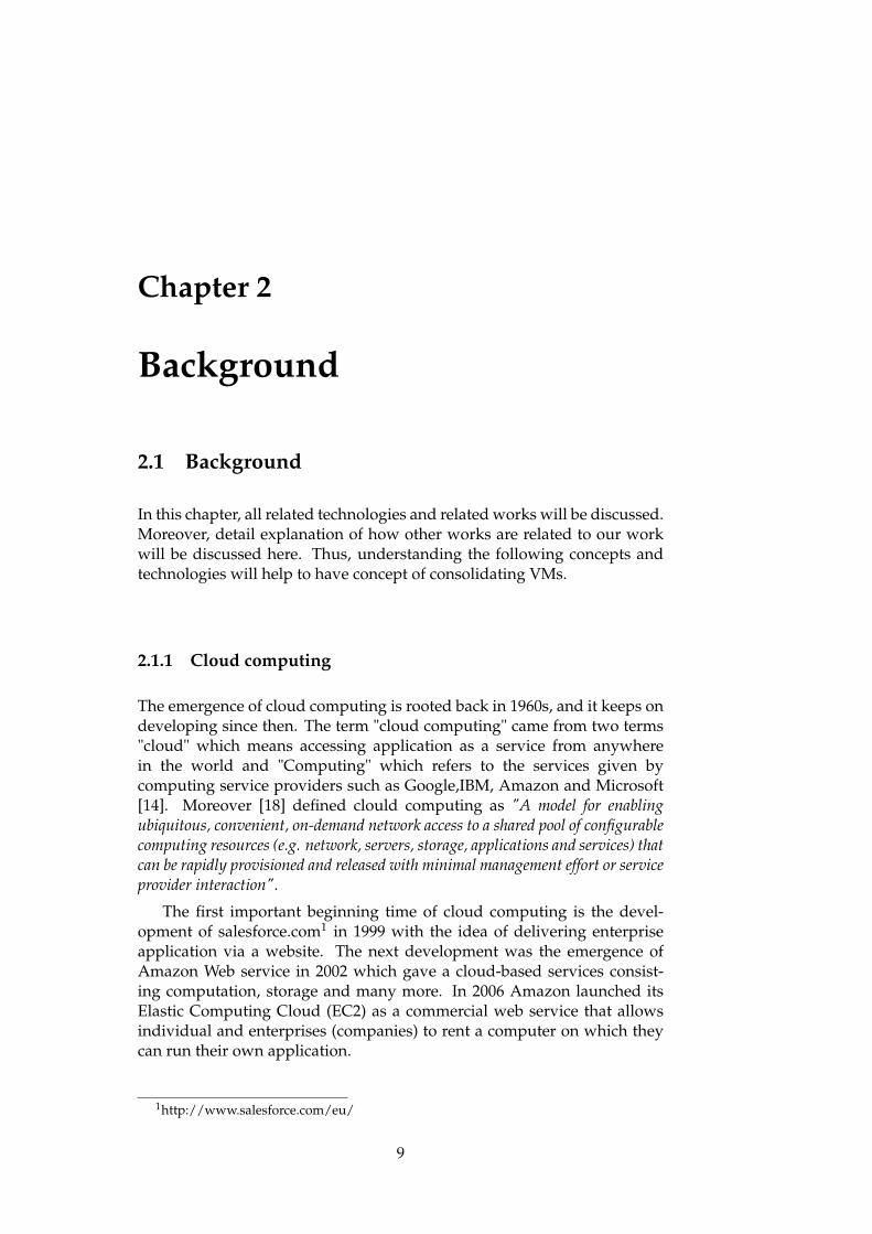
Figure 2.1: Service Layer
Recently cloud computing is giving computational services such asSoftware as a service (SaaS), a cloud computing model which givesservice as a software or applications via network, typically the Internetby service providers for example Goggle Apps, Microsoft Office 365;Platform as a service (PaaS), is a model in which running an applicationbecomes possible even with out having a hardware to run it. For exampleAWS Elastic Beanstalk, Heroku, Force.com, Google App Engine, ApacheStratos ; and Infrastructure as a service (IaaS), is a service model inwhich computational resources provided is of virtual type. For exampleAmazon EC2, Windows Azure, Rackspace, Google Compute Engine.Thus, customers can build their own platform on the provided virtualinfrastructure[17]. Managing these services and their infrastructuresbecome important in all IT arena. In addition to the service modelsmentioned above, [18] described the characteristics of cloud computing asfollows:
• On-Demand self-service- a consumers have the capability of comput-ing with intervention of service providers.
• Broad network access- The use of mobile phones, tablets, laptops andworkstations through standard mechanism over the network.
• Resource pooling- service provider’s resources are pooled by severalconsumers based on their demands. The location of these resourcesare not known by consumers.
• Rapid elasticity- Scalability for provisioning are almost unlimited.
• Measured service- cloud systems control and optimize resourceusage.
As they discussed further cloud computing can be deployed in one ofthe following ways:
10
CHAPTER 2. BACKGROUND 2.1. BACKGROUND
• Private clouds- such clouds are provisioned for exclusive use byorganization having multiple users. It can be managed and controlledby an organization or providers.
• Community cloud- such clouds are used by a group of people,specific community of users have shared concerns.
• Public cloud-provisioned to general public such as business, aca-demic and the likes
• Hybrid cloud- are combination of the above mentioned clouds.
Thus cloud computing management emerged for the sake of managingcloud computing infrastructures and services. In-addition to Amazon EC22
other cloud management systems such as Euclaptus3, CloudStack4 andOpenStack5 have emerged.
2.1.2 Virtualization
In computing technologies, virtualization is creating a virtual versionrather than real (actual) version of devices such as hard disks, servers,network and even operating systems and many more[28]. There are threetypes of virtualization:
• para virtualization, in which a hardware environment is not simu-lated; however, the guest programs are executed in their own isolateddomains;
• partial virtualization, in which some but not all of the targetenvironment is simulated; Some guest programs, therefore, may needmodifications to run in this virtual environment; and
• full virualization, in which almost complete simulation of the actualhardware to allow software, which typically consists of a guestoperating system, to run unmodified[30].Without virtualization ofdata centers, it wouldn’t have been possible to talk about virtualmachines (VMs). One of the benefits of virtualization is VMconoslidation for efficient use of electricity and other data centerresources.
2http://aws.amazon.com/ec2/3https://www.eucalyptus.com/4https://cloudstack.apache.org/5https://www.openstack.org/
11
2.1. BACKGROUND CHAPTER 2. BACKGROUND
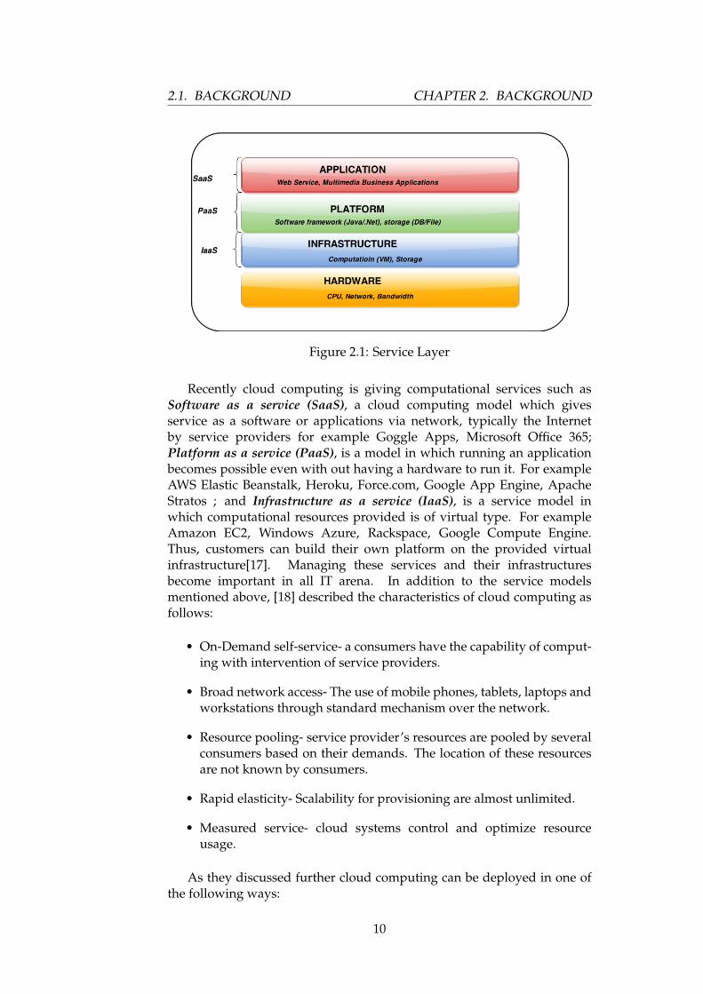
Figure 2.2: Virtualization Layer
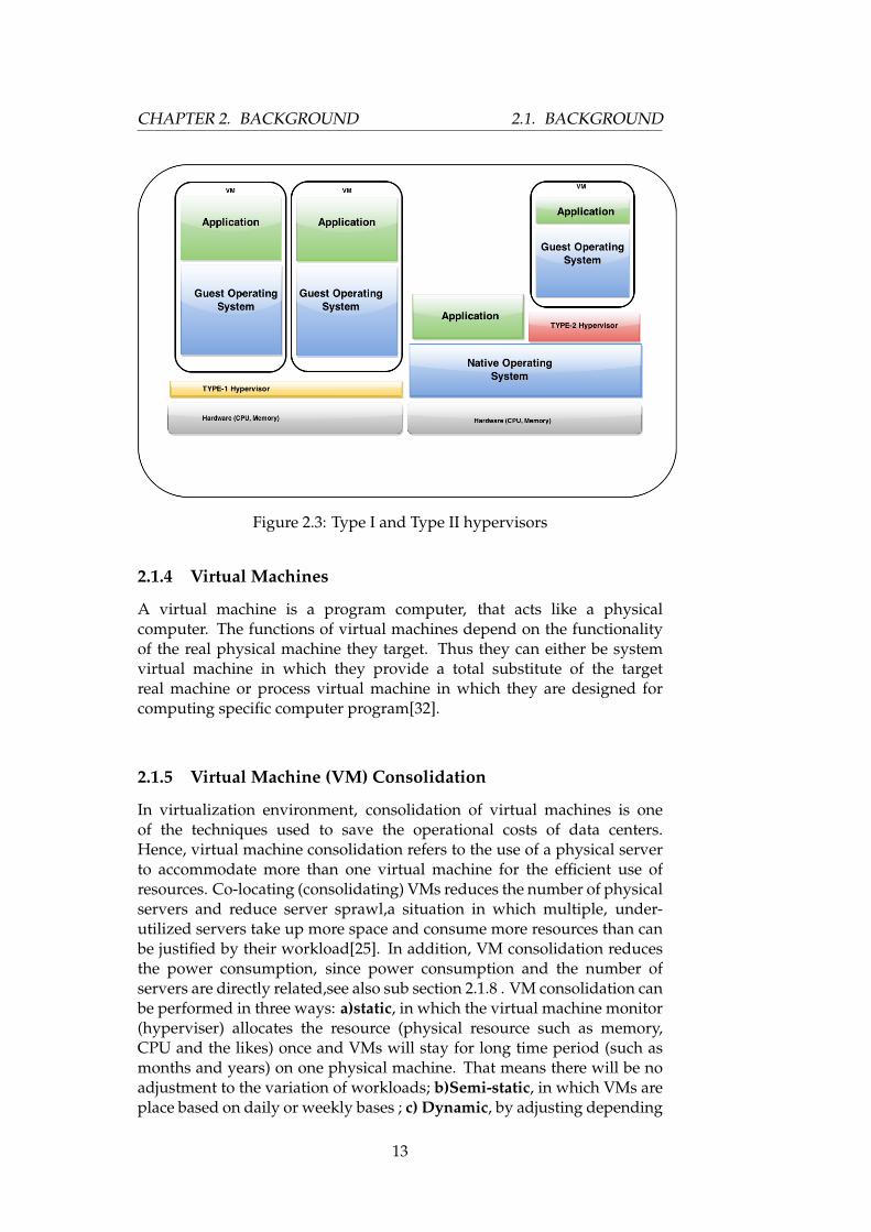
2.1.3 Hypervisor
A hypervisor is a software, firmware or hardware that creates and runsvirtual machines. It is also called virtual machine manager. Virtualmachine manager collects resource usage information, such as CPUutilization, memory consumption and so on of a physical machine. Thereare two types of hypervisors:
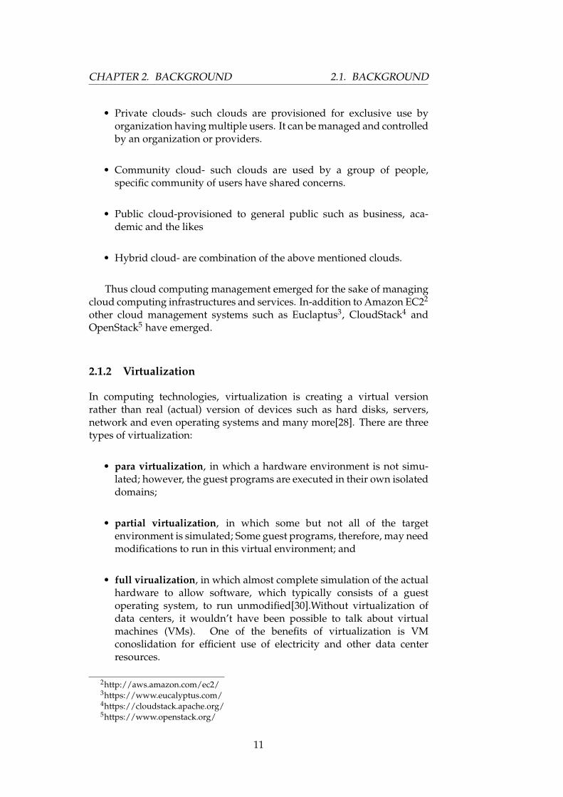
• 1) Naive or bare-metal hypervisors, also called Type I Hypervisor, inthis type of hypervisor software will be installed on the server as anoperating systems and resources are paravirtualized and forwardedto running virtual machines ; and
• 2) Hosted hypervisors, also called Type II hypervisor, in suchtype of hypervisors a software will be loaded on top of alreadyrunning operating system, for example installing virtual box on topof windows 8 or windows server 2008[21].
12
CHAPTER 2. BACKGROUND 2.1. BACKGROUND
Figure 2.3: Type I and Type II hypervisors
2.1.4 Virtual Machines
A virtual machine is a program computer, that acts like a physicalcomputer. The functions of virtual machines depend on the functionalityof the real physical machine they target. Thus they can either be systemvirtual machine in which they provide a total substitute of the targetreal machine or process virtual machine in which they are designed forcomputing specific computer program[32].
2.1.5 Virtual Machine (VM) Consolidation
In virtualization environment, consolidation of virtual machines is oneof the techniques used to save the operational costs of data centers.Hence, virtual machine consolidation refers to the use of a physical serverto accommodate more than one virtual machine for the efficient use ofresources. Co-locating (consolidating) VMs reduces the number of physicalservers and reduce server sprawl,a situation in which multiple, under-utilized servers take up more space and consume more resources than canbe justified by their workload[25]. In addition, VM consolidation reducesthe power consumption, since power consumption and the number ofservers are directly related,see also sub section 2.1.8 . VM consolidation canbe performed in three ways: a)static, in which the virtual machine monitor(hyperviser) allocates the resource (physical resource such as memory,CPU and the likes) once and VMs will stay for long time period (such asmonths and years) on one physical machine. That means there will be noadjustment to the variation of workloads; b)Semi-static, in which VMs areplace based on daily or weekly bases ; c) Dynamic, by adjusting depending
13
2.1. BACKGROUND CHAPTER 2. BACKGROUND
on the workload characteristics (Peak and off-peak utilization of resources)and make adjustment in hours and needs run-time placement algorithms .Dynamic VM consolidation helps in the efficient use of data centers [6] [26][14][7]. In order to consolidate VMs there are several processes that mustbe undertaken. These are, vm selection, vm placement and vm migration.
VM Selection
VM selection is one of the challenges of VM consolidation process. Itdeals with migrating VMs until the physical machine is considered tobe not overloaded. In VM selection process there are several policies tobe followed for effective accomplishment of the process. These policiesare discussed in detail by Heena Kaushar and et al.[3] as follows :a) Theminimum Migration Time Policy; b) the maximum Correlation Plicy; c) TheRandom Choice Plicy and; d)Highest Potential Growth (HPG). Moreover, itis also described in detail by [13][11] as follows:a)Local Regression;b)Inter-quartile Range;c) Median Absolute deviation.
VM Placement
The process of selecting the most suitable host for the virtual machine,when a virtual machine is deployed on a host, is known as virtual machineplacement, or simply placement. During placement, hosts are rated basedon the virtual machine’s hardware and resource requirements and theanticipated usage of resources. Host ratings also take into considerationthe placement goal: either resource maximization on individual hosts orload balancing among hosts. The administrator selects a host for the virtualmachine based on the host ratings.[27]
VM Migration
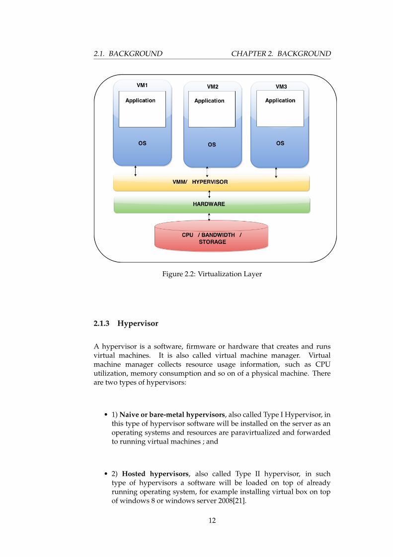
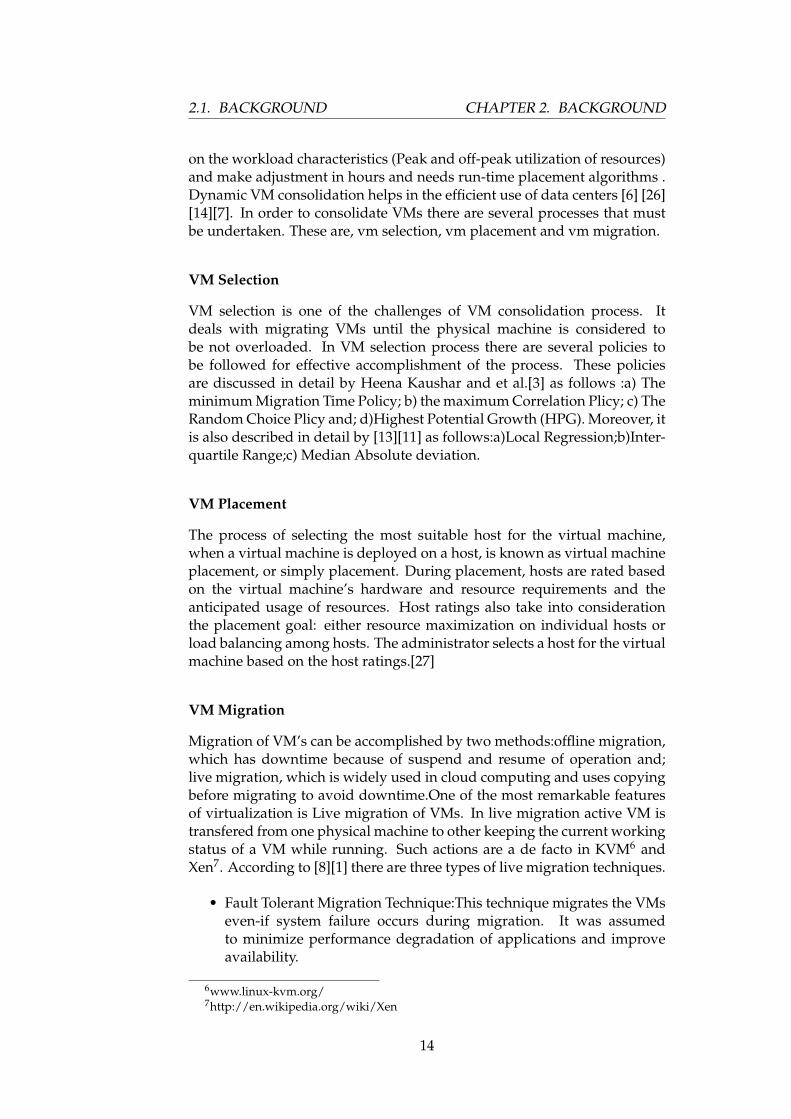
Migration of VM’s can be accomplished by two methods:offline migration,which has downtime because of suspend and resume of operation and;live migration, which is widely used in cloud computing and uses copyingbefore migrating to avoid downtime.One of the most remarkable featuresof virtualization is Live migration of VMs. In live migration active VM istransfered from one physical machine to other keeping the current workingstatus of a VM while running. Such actions are a de facto in KVM6 andXen7. According to [8][1] there are three types of live migration techniques.
• Fault Tolerant Migration Technique:This technique migrates the VMseven-if system failure occurs during migration. It was assumedto minimize performance degradation of applications and improveavailability.
6www.linux-kvm.org/7http://en.wikipedia.org/wiki/Xen
14
CHAPTER 2. BACKGROUND 2.1. BACKGROUND
• Load Balancing Migration Technique: This technique distributes loadacross the physical servers to improve the scalability of physical serv-ers. It helps in in minimizing the resource consumption, implementa-tion of fail-over, enhancing scalability, avoiding bottlenecks and overprovisioning of resources etc.
• Energy Efficient Migration Technique: The power consumption ofData center is mainly based on the utilization of the servers andtheir cooling systems. Thus, migration techniques that conserves theenergy of servers by optimum resource utilization is of focus.
Figure 2.4: Live Migration of VMs
Benefits of VM Consolidation:
• Reduce operational costs:Hardware cost: Efficient use resources reduces the number of resourcesused when consolidation are applied.Power Cooling cost: the effect of reduction in the use of physical re-sources such as servers and racks leads to reduction in power andcooling system in a data center.
• Easy backup- thanks to snapshot taking back up is very easy.
• Deployment advantage- redeploying is easy by enabling snapshots.
• Green environment: reduction in use of electricity favours to greenenvironment.
• Testing: Testing is very easy. Thanks to snapshot
• Server Sprawl-No over provisioning any more
• Decreased labour cost
• Reduced maintenance cost
Negatives of VM Consolidation
If proper management is not applied VM consolidation can end up in thefollowing disadvantages.
15
2.1. BACKGROUND CHAPTER 2. BACKGROUND
• Overheads:Migration and placement of VMs can cause impact onperformance of applications.This leads to overhead on network linkand CPU utilization.
• Performance problem: VM consolidation can cause performanceproblem due to contention that arises from using the same physicaresource such as CPU, memory and others.
• Single Point of failure: The main goal of VM consolidation is to packas many VMs to a single physical server as possible. If necessaryactions such as taking snapshots and others are not taken it can causesystem failure.
Beside the above mentioned negatives, VM consolidation benefitoutweighs and large data centers are using it increasingly.
2.1.6 Bin Packing
Bin packing problem is a combinatorial NP-hard problem, in which objectsof different volumes must be packed into a finite number of bins in a waythat minimizes the number of bins used[31].
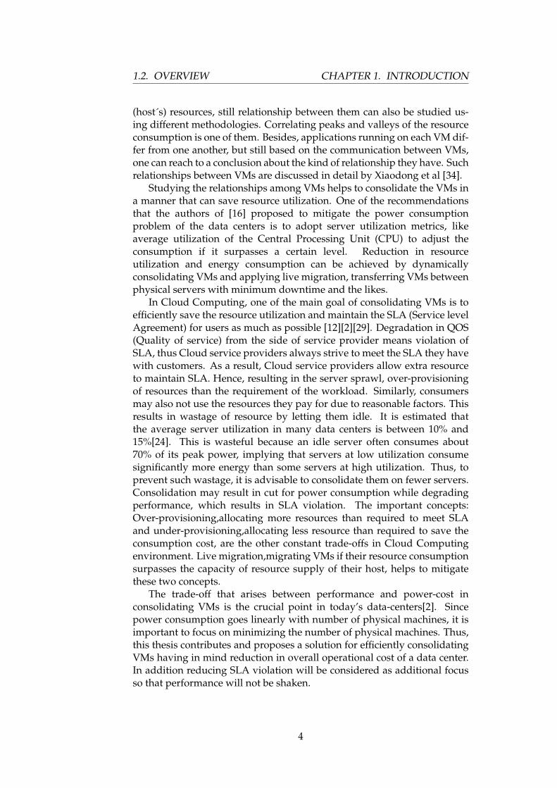
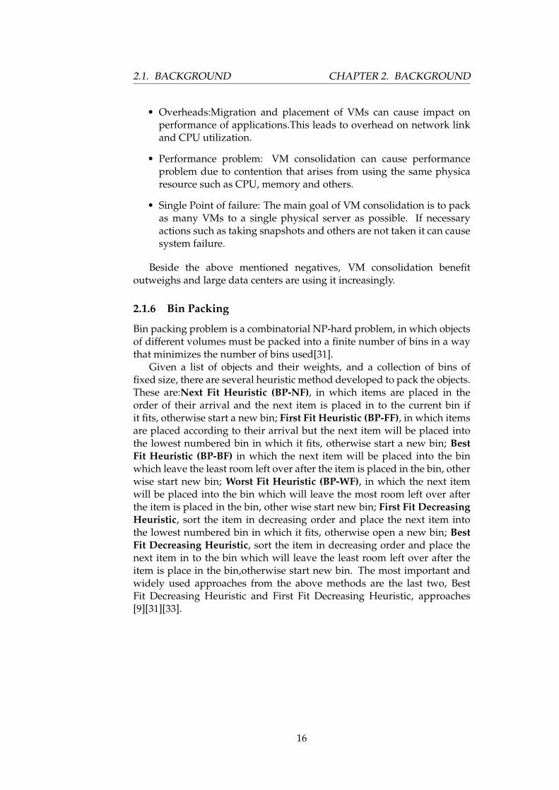
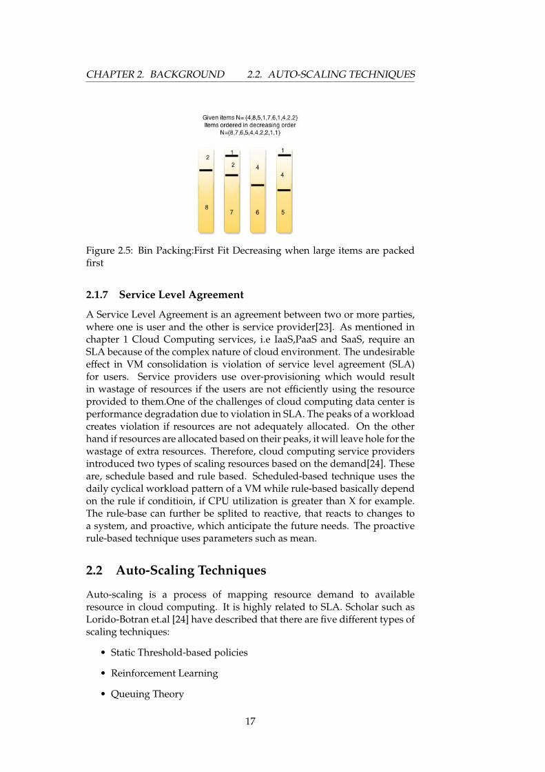
Given a list of objects and their weights, and a collection of bins offixed size, there are several heuristic method developed to pack the objects.These are:Next Fit Heuristic (BP-NF), in which items are placed in theorder of their arrival and the next item is placed in to the current bin ifit fits, otherwise start a new bin; First Fit Heuristic (BP-FF), in which itemsare placed according to their arrival but the next item will be placed intothe lowest numbered bin in which it fits, otherwise start a new bin; BestFit Heuristic (BP-BF) in which the next item will be placed into the binwhich leave the least room left over after the item is placed in the bin, otherwise start new bin; Worst Fit Heuristic (BP-WF), in which the next itemwill be placed into the bin which will leave the most room left over afterthe item is placed in the bin, other wise start new bin; First Fit DecreasingHeuristic, sort the item in decreasing order and place the next item intothe lowest numbered bin in which it fits, otherwise open a new bin; BestFit Decreasing Heuristic, sort the item in decreasing order and place thenext item in to the bin which will leave the least room left over after theitem is place in the bin,otherwise start new bin. The most important andwidely used approaches from the above methods are the last two, BestFit Decreasing Heuristic and First Fit Decreasing Heuristic, approaches[9][31][33].
16
CHAPTER 2. BACKGROUND 2.2. AUTO-SCALING TECHNIQUES
Figure 2.5: Bin Packing:First Fit Decreasing when large items are packedfirst
2.1.7 Service Level Agreement
A Service Level Agreement is an agreement between two or more parties,where one is user and the other is service provider[23]. As mentioned inchapter 1 Cloud Computing services, i.e IaaS,PaaS and SaaS, require anSLA because of the complex nature of cloud environment. The undesirableeffect in VM consolidation is violation of service level agreement (SLA)for users. Service providers use over-provisioning which would resultin wastage of resources if the users are not efficiently using the resourceprovided to them.One of the challenges of cloud computing data center isperformance degradation due to violation in SLA. The peaks of a workloadcreates violation if resources are not adequately allocated. On the otherhand if resources are allocated based on their peaks, it will leave hole for thewastage of extra resources. Therefore, cloud computing service providersintroduced two types of scaling resources based on the demand[24]. Theseare, schedule based and rule based. Scheduled-based technique uses thedaily cyclical workload pattern of a VM while rule-based basically dependon the rule if conditioin, if CPU utilization is greater than X for example.The rule-base can further be splited to reactive, that reacts to changes toa system, and proactive, which anticipate the future needs. The proactiverule-based technique uses parameters such as mean.
2.2 Auto-Scaling Techniques
Auto-scaling is a process of mapping resource demand to availableresource in cloud computing. It is highly related to SLA. Scholar such asLorido-Botran et.al [24] have described that there are five different types ofscaling techniques:
• Static Threshold-based policies
• Reinforcement Learning
• Queuing Theory
17
2.3. DATA CENTER CHAPTER 2. BACKGROUND
• Control Theory
• Time Series Analysis
2.2.1 CPU Consumption and Power Relationship
In a data center it is difficult to conclude that CPU consumption and powerusage are proportional. Since all processors (for example CPU,cooling fanand others) have their own energy consumption pattern. Studies showthat servers need up to 70% of their maximum power consumption evenat their low utilization level[8][13]. Thus, It can be concluded that thegreater the CPU utilization the greater the power consumption. It wasexperimentally shown that the power consumption and CPU utilizationhave linear relationship by [19][10].
2.2.2 Dynamic Voltage and Frequency Scaling
Dynamic Voltage and Frequency scaling (DVFS) is a power managementtechnique by modern processors to achieve energy efficiency. It is firstutilized for mobiles computing but later on it is utilized for energyconsumption in cluster of computers. It dynamically scales the supplyvoltage level of the CPU so as to provide circuit speed to process the systemworkload while meeting total computation time, which in effect reduceenergy wastage[5]. As stated in chapter 1 under section 1.5 (The goal ofthe thesis), one of the important achievements of consolidating VMs isreducing the energy wastage by shutting down the idle resource (server)mainly by using the technique under discussion.
2.3 Data Center
Data center can be called a house of computer systems and componentsthat make up organization’s main body. In generailized term, a data center"is a centralized repository, either physical or vitural, for the storage, management,and dissemintaion of data and information organized around a aprticulay body ofknowledge."Margareth Rouse (whatis.com) accessed 14.04.2015
2.4 Cloud Data Center
As cloud computing is the industry term for delivering hosted services overa network or the internet. It treats computing as a service rather than aproduct, enabling users to access and share a wide variety of applications,data, and resources through an interface such as their web browser[17].Compared to traditional data center, cloud data center has decreased costsof infrastructure, flexibility to workload than tradition data center andmany other more.
18
CHAPTER 2. BACKGROUND 2.5. COVARIANCE
2.5 Covariance
Covariance is a measure of how two variables act together. It has beenobserved that those VMs that have covariance greater than 0 as high-variance and those with less than 0 are considered low-variance.
2.6 Correlation
Correlation is a normailized covariance. Figure 3.3 shows the correlationbetween VMs in the data set. Many studies have shown that consolidatingbased on correlation will help for efficient consolidation. Correlationstandardizes the measure of interdependence between two variables and,consequently, tells how closely the two variables change. The correlationcoefficient, will always take on a value between 1 and – 1. if it is close to -1it means the correlation is strongly negatively correlated, i.e if one variableincreases the other variable decreases. If it is 0 then it means there is norelationship between the variables. If it is larger than one then it meansthey are positively correlated, i.e as one variable increase the other variablealso increases. A good candidate for VM consolidation is then negativelycorrelated VMs.
19
2.7. RELATED WORKS CHAPTER 2. BACKGROUND
2.7 Related works
Similar works has been conducted by many research communities ondynamic VM consolidation, and the focus of many of them were toreduce resource consumption in data center, mainly power consumption.Cost reduction regarding power consumption and maximizing the serverresource utilization were basically done by increasing packing efficiencyof VMs and minimizing the number of used servers. In order to achievethe efficiency of VM consolidation different researchers approached it in somany different ways.
The authors of [14] proposes allocation and selection policy for thedynamic virtual machine (VM) consolidation in virtualized data centersto reduce energy consumption and SLA violation. Mean and standarddeviation of CPU utilization for VMs were used to determine if thehosts are overloaded or not. Besides, they used the positive maximumcorrelation coefficient to select VMs from those overloading hosts formigration. Similar to our work mean are used to determine if the PMmachines are overloaded, but our work uses variance and covarianceinstead of standard deviation in addition to mean. In addition the proposedallocation and selection policy uses probability to decide whether to put theVM on the PM.
Beloglazov and Buyya et al. in their works [11] [13]have implementedan energy-aware resource allocation heuristic for VMs consolidation. Theyproposed fixed threshold to migrate VMs on[11] and variable thresholdin[13] in addition to new VM allocation and selection policies. The authorsof [26] propose a joint-VM provisioning approach in which multiple VMsare consolidated and provisioned together, based on an estimate of theiraggregate capacity needs. Their work looks aw-some in reducing SLAviolation, but complicated.
Bin packing algorithm was used by[4] assuming the resource usagewill remain constant, which seems similar to what we have applied in ouralgorithm. They also characterize the resource usage dynamics by principalcomponents, and propose to place VMs using variance reduction.
20

CHAPTER 2. BACKGROUND 2.7. RELATED WORKS
21

2.7. RELATED WORKS CHAPTER 2. BACKGROUND
22
Chapter 3
Methodology
This chapter describes the experimental design, the set up and implement-ation part of the approach to pursue the goal of the thesis. Moreover, howto apply the designed algorithms will be discussed under this chapter. Dif-ferent approaches to tackle the problem statement of the paper will be dis-cussed here. Generally,explanation of how and why the approaches underdiscussion are chosen will be discussed under this chapter.
3.1 Objective of the experiment
The objectives of the experiment as mentioned briefly under the introduc-tion part of this thesis is exploring how to improve VM consolidation byaccessing time dependent behaviour of VMs and multiplex the VMs to re-duce the total operational cost of a data center. The introduction of efficientalgorithm that dynamically consolidate VMs with out violating SLA in adata center is of a focus. As discussed in previous chapter, reduction inoperational cost of a data center includes:
• Reduction of energy consumption in the data center
• Effective utilization of physical machine
• Computational costs
• Network devices costs
• Environment costs(because of carbon emission)
• Cooling costs and the likes.
23
3.2. SYSTEM ARCHITECTURE CHAPTER 3. METHODOLOGY
3.2 System Architecture
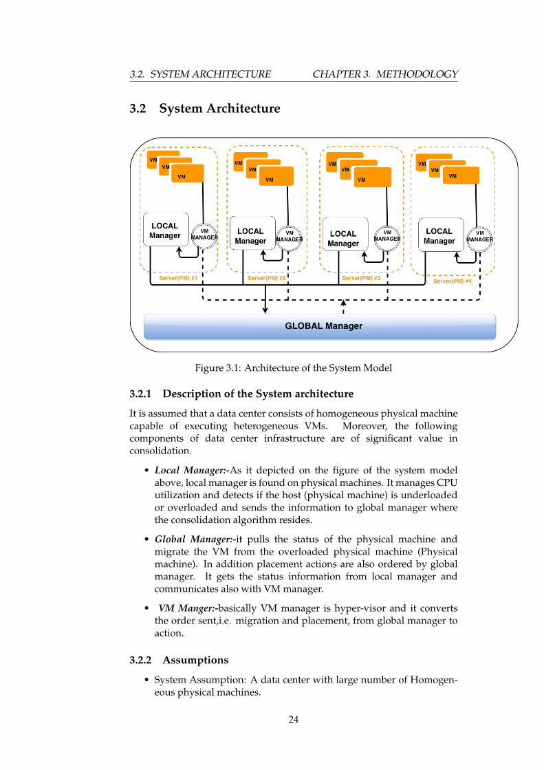
Figure 3.1: Architecture of the System Model
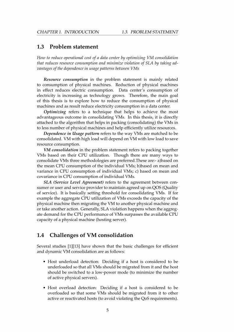
3.2.1 Description of the System architecture
It is assumed that a data center consists of homogeneous physical machinecapable of executing heterogeneous VMs. Moreover, the followingcomponents of data center infrastructure are of significant value inconsolidation.
• Local Manager:-As it depicted on the figure of the system modelabove, local manager is found on physical machines. It manages CPUutilization and detects if the host (physical machine) is underloadedor overloaded and sends the information to global manager wherethe consolidation algorithm resides.
• Global Manager:-it pulls the status of the physical machine andmigrate the VM from the overloaded physical machine (Physicalmachine). In addition placement actions are also ordered by globalmanager. It gets the status information from local manager andcommunicates also with VM manager.
• VM Manger:-basically VM manager is hyper-visor and it convertsthe order sent,i.e. migration and placement, from global manager toaction.
3.2.2 Assumptions
• System Assumption: A data center with large number of Homogen-eous physical machines.
24
CHAPTER 3. METHODOLOGY 3.3. DATA
• Resource assumption: CPU utilization demand of VM for the firsttime are assumed to be 100%
• Approach/algorithm: VM consolidation is considered as analoguesto bin packing, which is an NP-hard problem. Therefore thealgorithm used was heuristic greedy FFD algorithm that helps toreduce the number of physical machines utilized and SLA violation.
• Connection: It is assumed that all infrastructures are interconnected.
• Distribution: All Virtual machines (VMs) are considered as independ-ent variable and follow normal distribution in stochastic approaches.
• Capacity of physical machine: in this paper it is assumed thatcapacity means the average amount of instructions that a physicalmachine can compute and or the average amount of resource demandof a VM. Though it is measured in hertz (hz) we simple put it ascapacity.
3.2.3 Tools
• Lenovo: Intel Core i7-3537U CPU @2.00 GHz 2.5 GHZRAM: 8GBOS: ubuntu
• R-studio: For ploting,
• Python:for scripting and simulation.
• Numpy: a Python library to compute all the necessary computationalmeasures,such as mean, standard deviation,variance, covariance ...
• text editors: Nano,Latex
3.3 Data
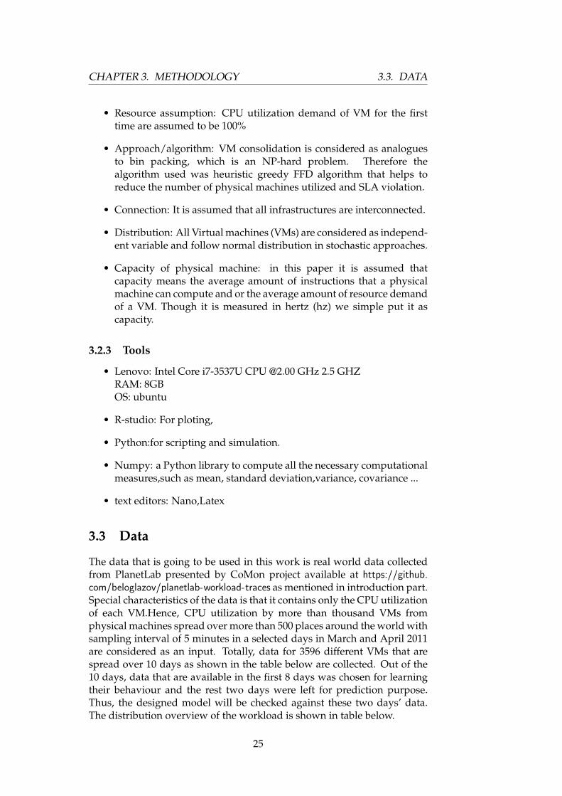
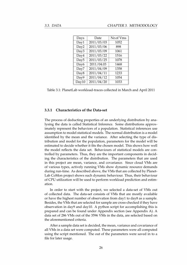
The data that is going to be used in this work is real world data collectedfrom PlanetLab presented by CoMon project available at https://github.com/beloglazov/planetlab-workload-traces as mentioned in introduction part.Special characteristics of the data is that it contains only the CPU utilizationof each VM.Hence, CPU utilization by more than thousand VMs fromphysical machines spread over more than 500 places around the world withsampling interval of 5 minutes in a selected days in March and April 2011are considered as an input. Totally, data for 3596 different VMs that arespread over 10 days as shown in the table below are collected. Out of the10 days, data that are available in the first 8 days was chosen for learningtheir behaviour and the rest two days were left for prediction purpose.Thus, the designed model will be checked against these two days’ data.The distribution overview of the workload is shown in table below.
25
3.3. DATA CHAPTER 3. METHODOLOGY
Days Date Nr.of VmsDay1 2011/03/03 1052Day2 2011/03/06 898Day3 2011/03/09 1061Day4 2011/03/22 1516Day5 2011/03/25 1078Day6 2011/04.03 1468Day7 2011/04/09 1358Day8 2011/04/11 1233Day9 2011/04/12 1054Day10 2011/04/20 1033
Table 3.1: PlanetLab workload-traces collected in March and April 2011
3.3.1 Characteristics of the Data-set
The process of deducting properties of an underlying distribution by ana-lysing the data is called Statistical Inference. Some distributions approx-imately represent the behaviors of a population. Statistical inferences useassumption to model statistical models. The normal distribution is a modelidentified by the mean and the variance. After selecting the type of dis-tribution and model for the population, parameters for the model will beestimated to decide whether it fits the chosen model. This shows how wellthe model reflects the data set. Behaviours of statistical models are con-trolled by parameters. Thus, they are the important components in decid-ing the characteristics of the distribution. The parameters that are usedin this project are mean, variance, and covariance. Since cloud VMs areof various types, actively running VMs show dynamic resource demandsduring run-time. As described above, the VMs that are collected by Planet-Lab CoMon project shows such dynamic behaviour. Thus, their behaviourof CPU utilization will be used to perform workload prediction and estim-ation.
In order to start with the project, we selected a data-set of VMs outof collected data. The data-set consists of VMs that are mostly availableor have the highest number of observation from day1 to day8 as a sample.Besides, the VMs that are selected for sample are cross-checked if they haveobservation in day9 and day10. A python script for accomplishing this isprepared and can be found under Appendix section (see Appendix A). Adata set of 286 VMs out of the 3596 VMs in the data, are selected based onthe aforementioned criteria.
After a sample data set is decided, the mean, variance and covariance ofall VMs in a data set were computed. These parameters were all computedusing the script mentioned. The out of the parameters were saved in to afile for later usage.
26
CHAPTER 3. METHODOLOGY 3.4. EXPERIMENTAL SETUP
3.4 Experimental Setup
As it is mentioned earlier, our target system is IaaS (Infrastructue as aService) and the system architecture is as shown in figure 3.1 above. itis difficult to conduct experiments with real infrastructure, however theimportance of evaluating the approaches outlined with their correspondingalgorithms on virtualized data center is huge. The cost and time frameallowed to conduct the experiment are some of various factors that arehinderance to experiment it with real infrastructure. Hence, simulation isthe best alternative at hand to mimic a data center.
The following procedures were followed to obtain results. A script thatcollects the data set will be run first. The script computes, all the necessaryinputs for bin-packing (i.e. mean, variance, and covariance. Next, thescript that applies first fit decreasing bin-packing to the selected data willbe run. In the scripts, physical machines are considered as bins and VMsare considered as items that are going to be place in the bin (see AppendixB, C, D for more). The result from first fit decreasing bin-packing algorithmof all approaches will be saved to a file. Each file contains the number ofphysical machines utilized to pack (consolidate) the VMs and also whichVMs are packed on which physical machine. These generated files from thescript run include the different scenarios used in the two last approaches(Variance and Covariance).Thus, there will be 14 files all together for thethree approaches, 2 files for only mean-based (1 for capacity 120 and theother for capacity 140), 6 files for variance-based (3 for each of capacity 120and 140 with scenarios (α=0.05, 0.5, 0.95), and 6 files for covariance-based.Moreover, a script that collects the total number of SLA violation will be runat the end. This script collects those VMs that has probability of exceedingthe agreed up on service level agreement (SLA).
The result obtained will be shown in the next chapter and evaluationand analysis will be given in the corresponding chapter.
3.4.1 Approaches for VM Consolidation
In order to achieve our goal, we conducted three different approaches.These Approaches are:-
• Deterministic Approach
• Stochastic approach I
• Stochastic approach II
Deterministic Approach
In deterministic approach we consider only mean to consolidate the VMs.Mean measures the central tendency of a probability distribution or of arandom variable in a distribution. Such parameters are import to considerwhen we think of consolidation. Under this category the mean values of theCPU utilization of each VMs in a data set were taken. By mean value we
27
3.4. EXPERIMENTAL SETUP CHAPTER 3. METHODOLOGY
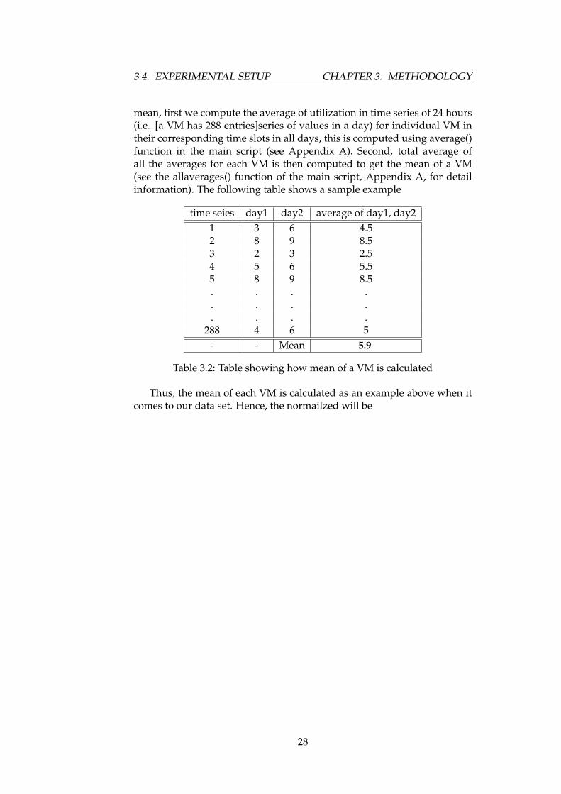
mean, first we compute the average of utilization in time series of 24 hours(i.e. [a VM has 288 entries]series of values in a day) for individual VM intheir corresponding time slots in all days, this is computed using average()function in the main script (see Appendix A). Second, total average ofall the averages for each VM is then computed to get the mean of a VM(see the allaverages() function of the main script, Appendix A, for detailinformation). The following table shows a sample example
time seies day1 day2 average of day1, day21 3 6 4.52 8 9 8.53 2 3 2.54 5 6 5.55 8 9 8.5. . . .. . . .. . . .
288 4 6 5- - Mean 5.9
Table 3.2: Table showing how mean of a VM is calculated
Thus, the mean of each VM is calculated as an example above when itcomes to our data set. Hence, the normailzed will be
28
CHAPTER 3. METHODOLOGY 3.4. EXPERIMENTAL SETUP
Generally, mean of individual VMs in our data-set of 286 VMs will beas follows
µi =1
Di ∗ 288
288
∑j=1
∑d∈Di
Xi jd (3.1)
where, Xi jd is observations for VMi at time stamp j and day d and Di isdays with observation for VMi
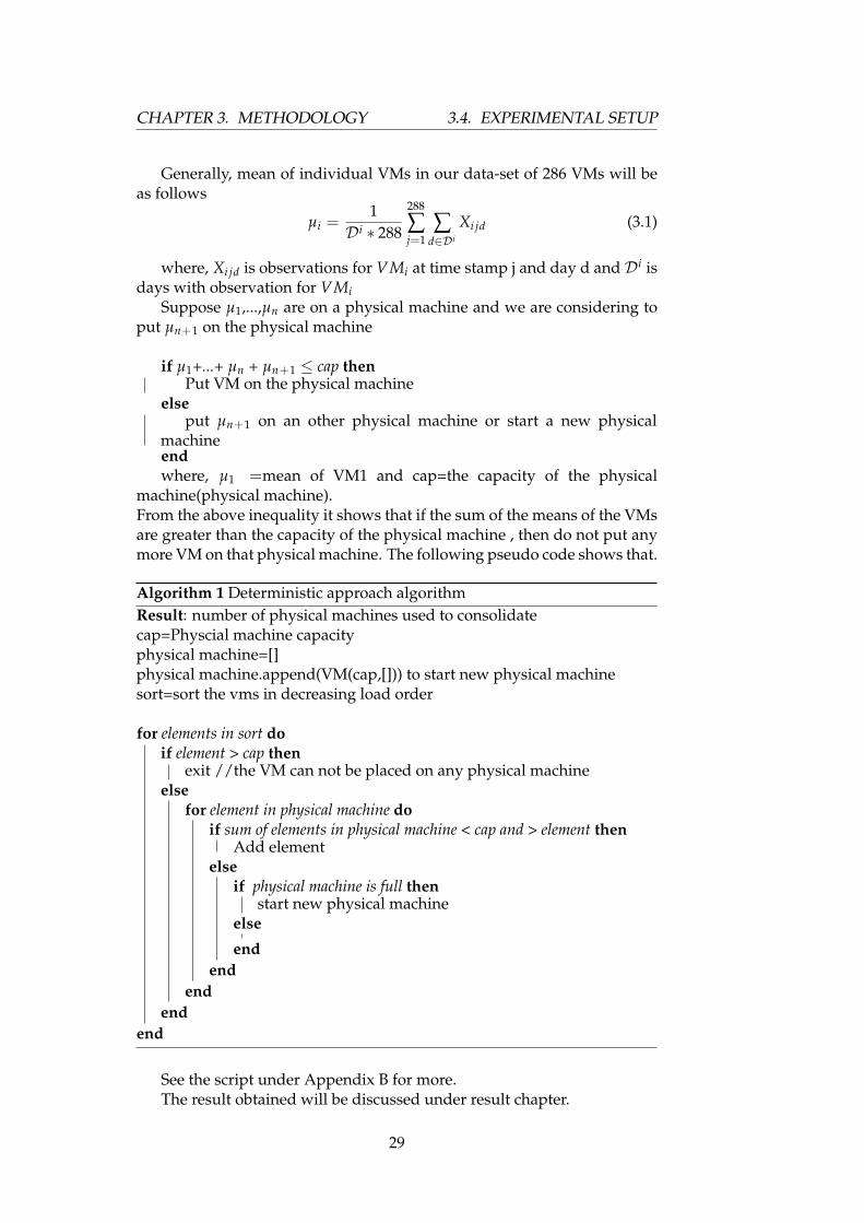
Suppose µ1,...,µn are on a physical machine and we are considering toput µn+1 on the physical machine
if µ1+...+ µn + µn+1 ≤ cap thenPut VM on the physical machine
elseput µn+1 on an other physical machine or start a new physical
machineendwhere, µ1 =mean of VM1 and cap=the capacity of the physical
machine(physical machine).From the above inequality it shows that if the sum of the means of the VMsare greater than the capacity of the physical machine , then do not put anymore VM on that physical machine. The following pseudo code shows that.
Algorithm 1 Deterministic approach algorithmResult: number of physical machines used to consolidatecap=Physcial machine capacityphysical machine=[]physical machine.append(VM(cap,[])) to start new physical machinesort=sort the vms in decreasing load order
for elements in sort doif element > cap then
exit //the VM can not be placed on any physical machineelse
for element in physical machine doif sum of elements in physical machine < cap and > element then
Add elementelse
if physical machine is full thenstart new physical machine
else
endend
endend
end
See the script under Appendix B for more.The result obtained will be discussed under result chapter.
29
3.4. EXPERIMENTAL SETUP CHAPTER 3. METHODOLOGY
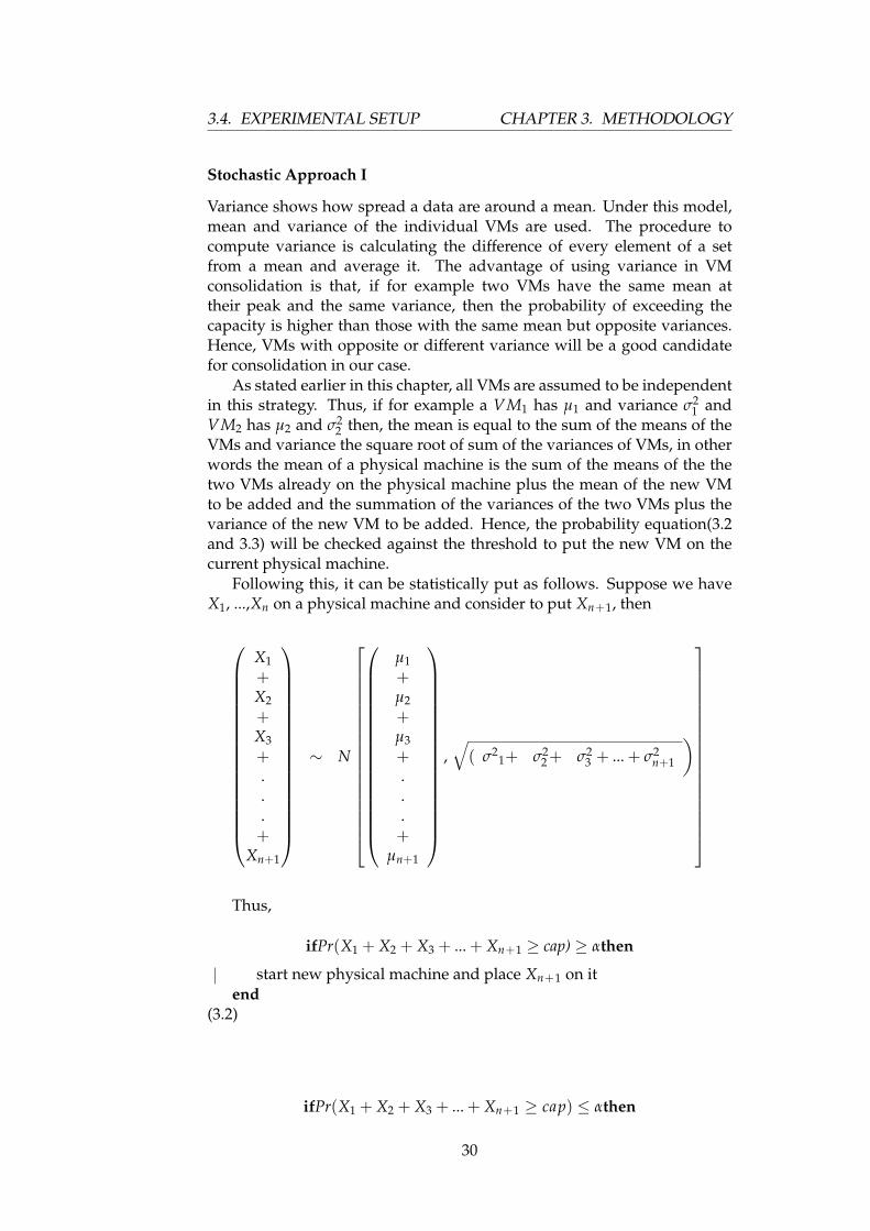
Stochastic Approach I
Variance shows how spread a data are around a mean. Under this model,mean and variance of the individual VMs are used. The procedure tocompute variance is calculating the difference of every element of a setfrom a mean and average it. The advantage of using variance in VMconsolidation is that, if for example two VMs have the same mean attheir peak and the same variance, then the probability of exceeding thecapacity is higher than those with the same mean but opposite variances.Hence, VMs with opposite or different variance will be a good candidatefor consolidation in our case.
As stated earlier in this chapter, all VMs are assumed to be independentin this strategy. Thus, if for example a VM1 has µ1 and variance σ2
1 andVM2 has µ2 and σ2
2 then, the mean is equal to the sum of the means of theVMs and variance the square root of sum of the variances of VMs, in otherwords the mean of a physical machine is the sum of the means of the thetwo VMs already on the physical machine plus the mean of the new VMto be added and the summation of the variances of the two VMs plus thevariance of the new VM to be added. Hence, the probability equation(3.2and 3.3) will be checked against the threshold to put the new VM on thecurrent physical machine.
Following this, it can be statistically put as follows. Suppose we haveX1, ...,Xn on a physical machine and consider to put Xn+1, then
X1+X2+X3+...+
Xn+1
∼ N
µ1+µ2+µ3+...+
µn+1
,√( σ2
1+ σ22+ σ2
3 + ... + σ2n+1
)
Thus,
ifPr(X1 + X2 + X3 + ... + Xn+1 ≥ cap) ≥ αthen
start new physical machine and place Xn+1 on itend
(3.2)
ifPr(X1 + X2 + X3 + ... + Xn+1 ≥ cap) ≤ αthen
30
CHAPTER 3. METHODOLOGY 3.4. EXPERIMENTAL SETUP
place Xn+1 with X1, ..., Xn
end(3.3)
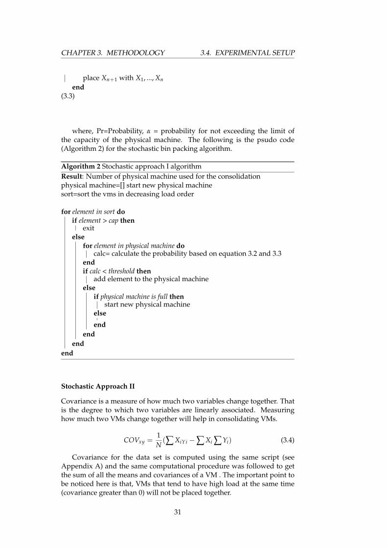
where, Pr=Probability, α = probability for not exceeding the limit ofthe capacity of the physical machine. The following is the psudo code(Algorithm 2) for the stochastic bin packing algorithm.
Algorithm 2 Stochastic approach I algorithmResult: Number of physical machine used for the consolidationphysical machine=[] start new physical machinesort=sort the vms in decreasing load order
for element in sort doif element > cap then
exitelse
for element in physical machine docalc= calculate the probability based on equation 3.2 and 3.3
endif calc < threshold then
add element to the physical machineelse
if physical machine is full thenstart new physical machine
else
endend
endend
Stochastic Approach II
Covariance is a measure of how much two variables change together. Thatis the degree to which two variables are linearly associated. Measuringhow much two VMs change together will help in consolidating VMs.
COVxy =1N(∑ XiYi −∑ Xi ∑ Yi) (3.4)
Covariance for the data set is computed using the same script (seeAppendix A) and the same computational procedure was followed to getthe sum of all the means and covariances of a VM . The important point tobe noticed here is that, VMs that tend to have high load at the same time(covariance greater than 0) will not be placed together.
31
3.4. EXPERIMENTAL SETUP CHAPTER 3. METHODOLOGY
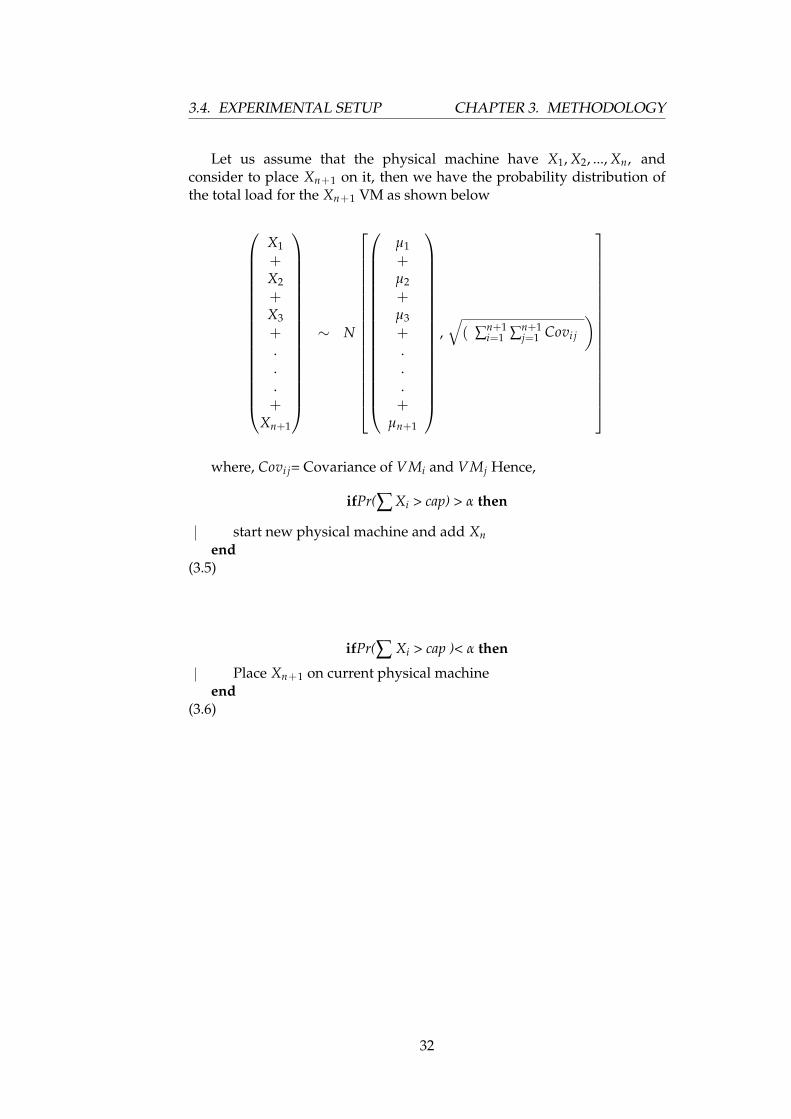
Let us assume that the physical machine have X1, X2, ..., Xn, andconsider to place Xn+1 on it, then we have the probability distribution ofthe total load for the Xn+1 VM as shown below
X1+X2+X3+...+
Xn+1
∼ N
µ1+µ2+µ3+...+
µn+1
,√( ∑n+1
i=1 ∑n+1j=1 Covi j
)
where, Covi j= Covariance of VMi and VMj Hence,
ifPr(∑ Xi > cap) > α then
start new physical machine and add Xnend
(3.5)
ifPr(∑ Xi > cap )< α then
Place Xn+1 on current physical machineend
(3.6)
32
CHAPTER 3. METHODOLOGY 3.5. POLICIES FOR SLA
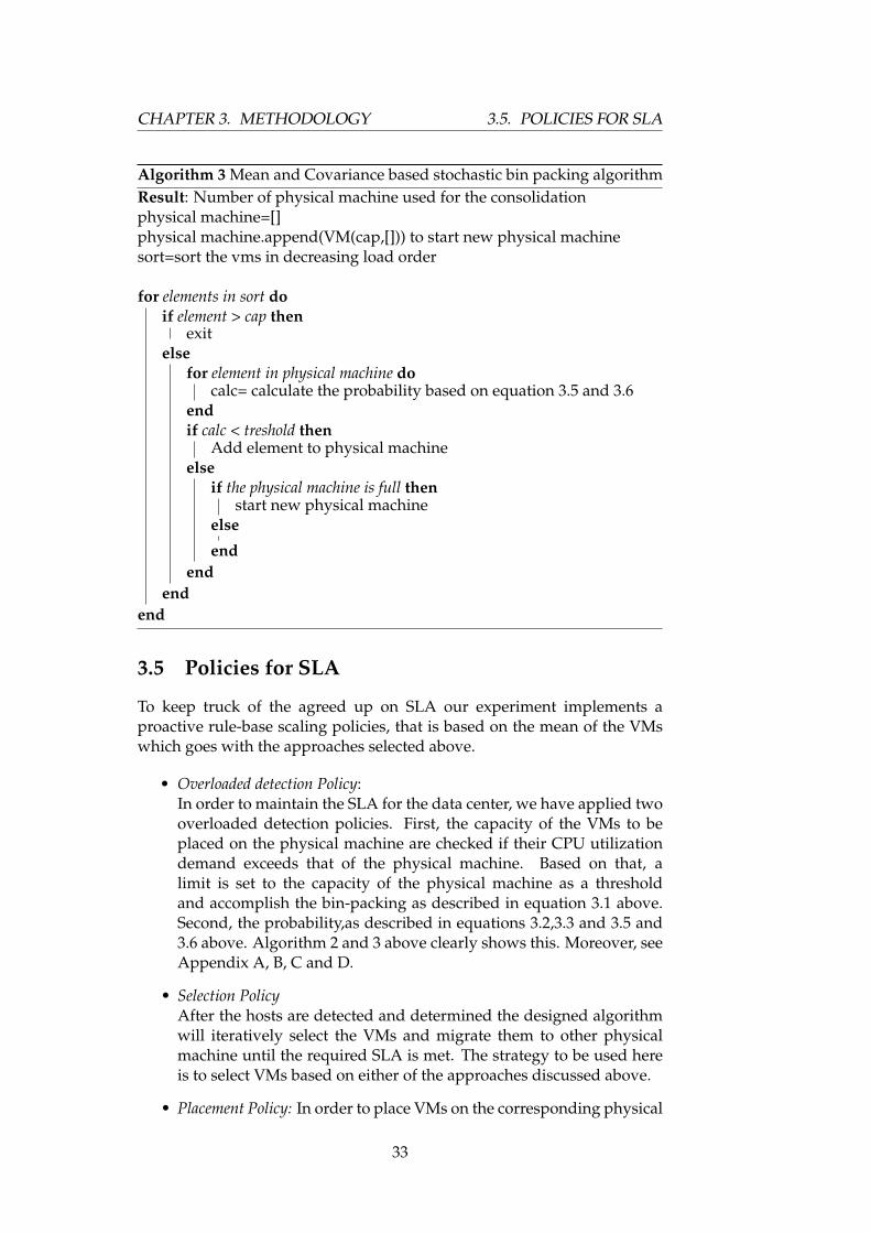
Algorithm 3 Mean and Covariance based stochastic bin packing algorithmResult: Number of physical machine used for the consolidationphysical machine=[]physical machine.append(VM(cap,[])) to start new physical machinesort=sort the vms in decreasing load order
for elements in sort doif element > cap then
exitelse
for element in physical machine docalc= calculate the probability based on equation 3.5 and 3.6
endif calc < treshold then
Add element to physical machineelse
if the physical machine is full thenstart new physical machine
else
endend
endend
3.5 Policies for SLA
To keep truck of the agreed up on SLA our experiment implements aproactive rule-base scaling policies, that is based on the mean of the VMswhich goes with the approaches selected above.
• Overloaded detection Policy:In order to maintain the SLA for the data center, we have applied twooverloaded detection policies. First, the capacity of the VMs to beplaced on the physical machine are checked if their CPU utilizationdemand exceeds that of the physical machine. Based on that, alimit is set to the capacity of the physical machine as a thresholdand accomplish the bin-packing as described in equation 3.1 above.Second, the probability,as described in equations 3.2,3.3 and 3.5 and3.6 above. Algorithm 2 and 3 above clearly shows this. Moreover, seeAppendix A, B, C and D.
• Selection PolicyAfter the hosts are detected and determined the designed algorithmwill iteratively select the VMs and migrate them to other physicalmachine until the required SLA is met. The strategy to be used hereis to select VMs based on either of the approaches discussed above.
• Placement Policy: In order to place VMs on the corresponding physical
33
3.5. POLICIES FOR SLA CHAPTER 3. METHODOLOGY
machine, the well know heuristic First Fit Decreasing bin-packingtechnique was used. Bins are considered as physical machines tohome the VMs and items are considered as VM to be guested on thephysical machines. In all the three approaches discussed above theplacement takes place based on the value the VMs have when thealgorithm runs. That is the values of a VM is double checked bothbefore placement and after placement. Thus, VM placement policywas introduced based on the capacity of the physical machine anddemand of the VM.
34

CHAPTER 3. METHODOLOGY 3.5. POLICIES FOR SLA
35

3.5. POLICIES FOR SLA CHAPTER 3. METHODOLOGY
36
Chapter 4
Results
In this section, the result obtained from the three approaches discussedin the previous chapter will be presented. As mentioned earlier, weconducted an experiment using three different approaches: deterministicapproach, stochastic approach I and stochastic approach II. The techniquesused for packing the VMs as mentioned was First Fit Decreasing bin-packing algorithm(see the algorithm at Appendix B,C and D). For thefirst approach, deterministic bin-packing based on mean of the VMs areused to consolidate the VMs. For the rest two approaches, stochastic binpacking algorithm was applied taking three different scenarios to comparethe approaches.
4.1 Evaluation Metrics
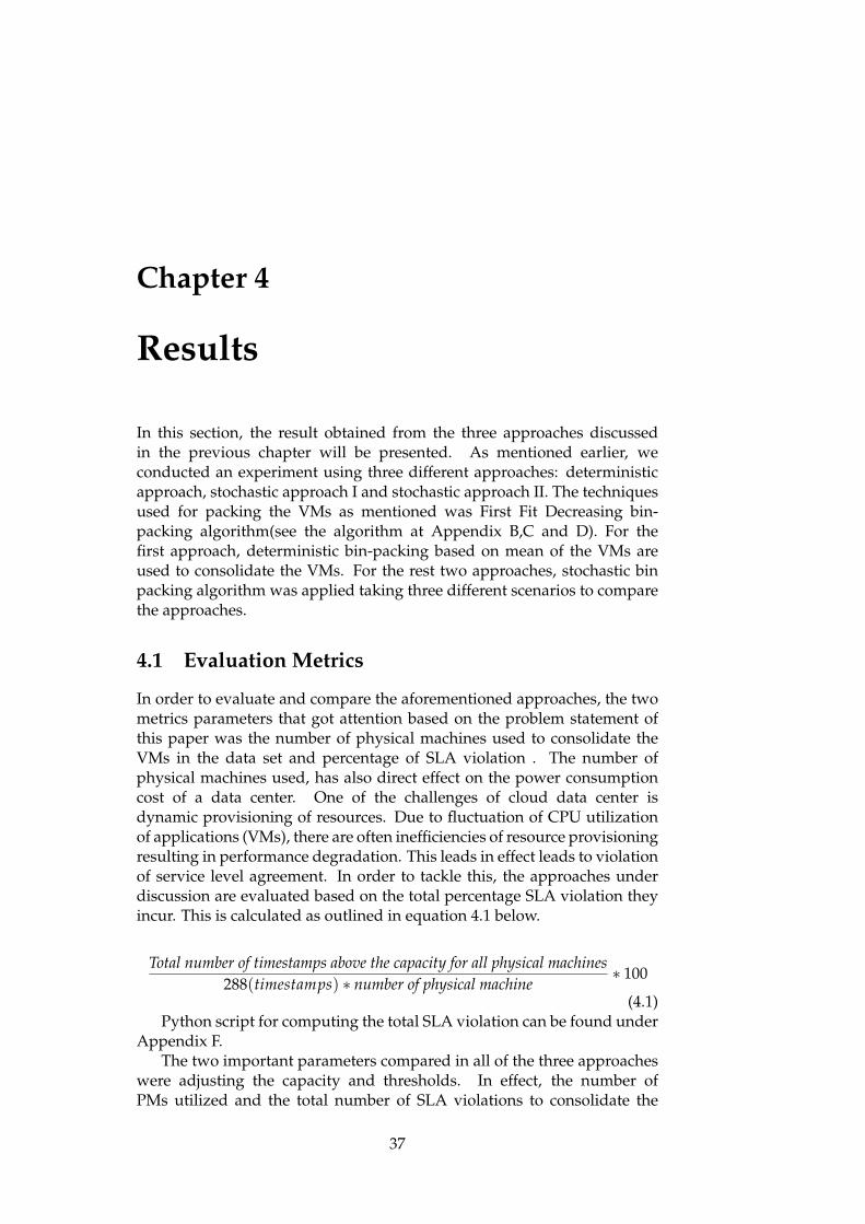
In order to evaluate and compare the aforementioned approaches, the twometrics parameters that got attention based on the problem statement ofthis paper was the number of physical machines used to consolidate theVMs in the data set and percentage of SLA violation . The number ofphysical machines used, has also direct effect on the power consumptioncost of a data center. One of the challenges of cloud data center isdynamic provisioning of resources. Due to fluctuation of CPU utilizationof applications (VMs), there are often inefficiencies of resource provisioningresulting in performance degradation. This leads in effect leads to violationof service level agreement. In order to tackle this, the approaches underdiscussion are evaluated based on the total percentage SLA violation theyincur. This is calculated as outlined in equation 4.1 below.
Total number of timestamps above the capacity for all physical machines288(timestamps) ∗ number of physical machine
∗ 100
(4.1)Python script for computing the total SLA violation can be found under
Appendix F.The two important parameters compared in all of the three approaches
were adjusting the capacity and thresholds. In effect, the number ofPMs utilized and the total number of SLA violations to consolidate the
37
4.2. NUMBER OF UTILIZED PMS CHAPTER 4. RESULTS
VMs will be evaulated. Thus, capacity was set to 120 and 140 for allapproaches. Additional parameters, considered as threshold, for the lasttwo approaches(i.e. stochastic approach I and II) was set to α=0.05, 0.5, and0.95. Results obtained are shown on the table 4.1 and 4.2 for number ofutilized PMs and 4.3 for total percentage of SLA violation.
4.2 Number of utilized PMs
Number of of used PMs, Mean-basedMethods Capacity=120 Capacity=140Mean 24 20
Table 4.1: Number of PMs used, Out put from Deterministic approach
——————————— Capacity = 120—–| ————-capacity =140Methods α =0.05 α =0.5 α =0.95 α =0.05 α =0.5 α =0.95Variance 27 24 20 23 20 18Covariance 27 24 18 23 20 16
Table 4.2: Number of PMs used by Stochastic Approach I and II
4.2.1 Number of VMs on each PM
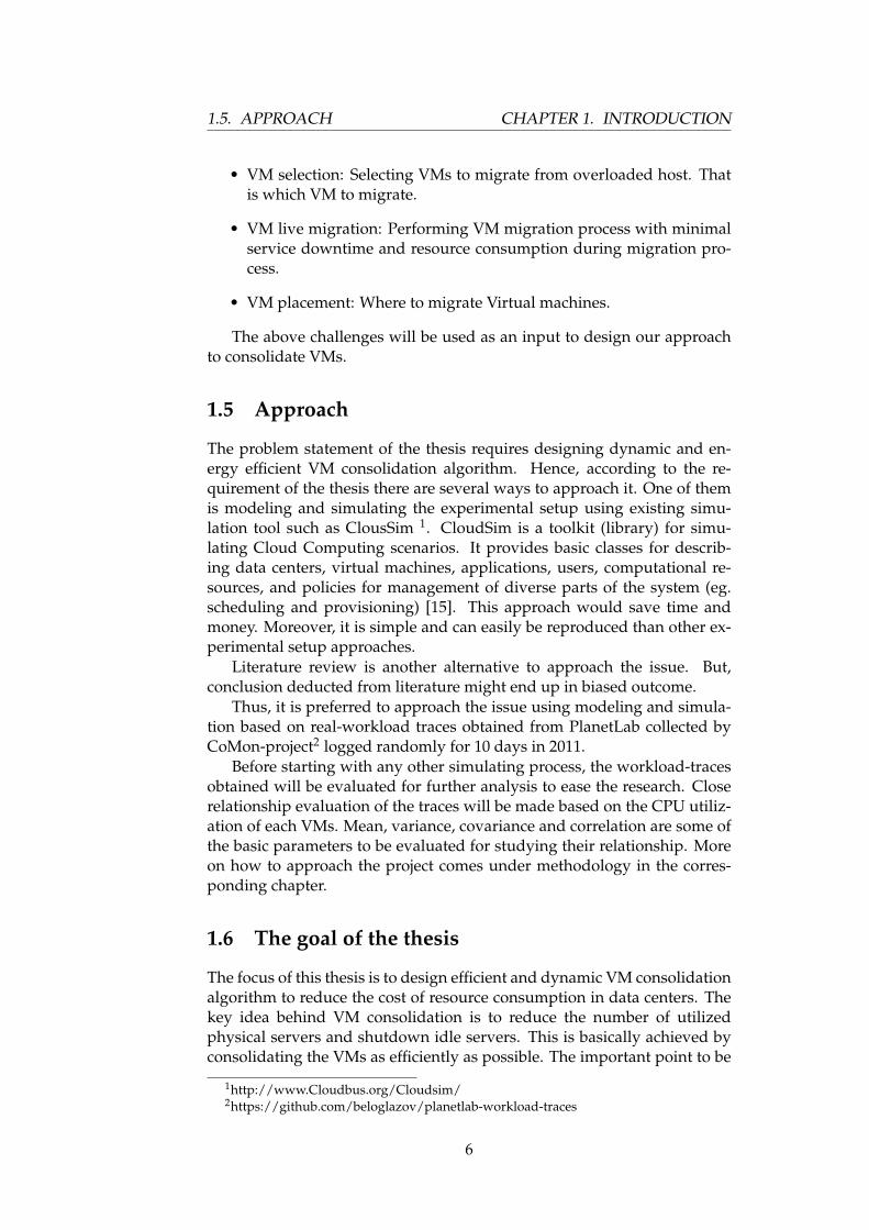
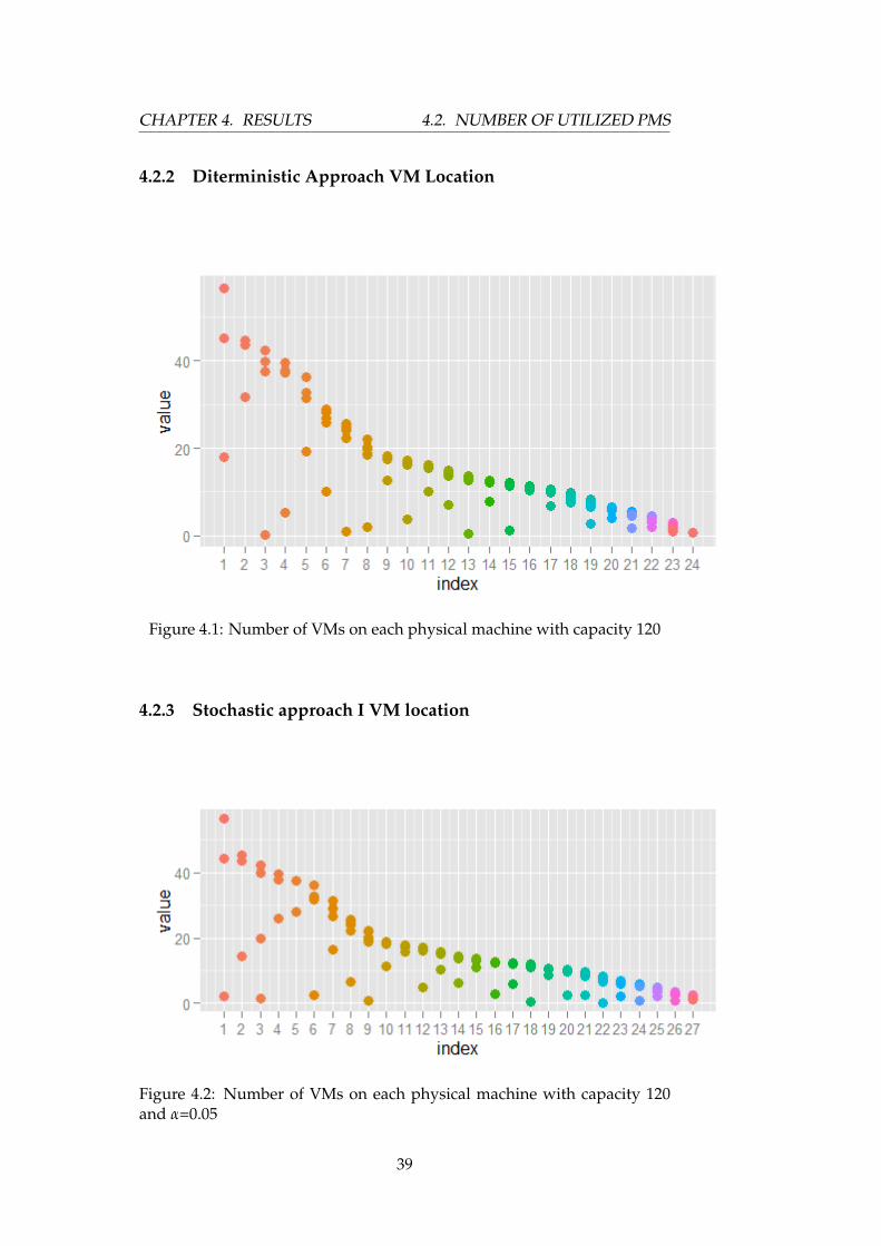
The following graphs shows details of how many VMs a PM(physicalmachine) can accommodate using the three different approaches. Forsimplicity of reading, in figures from Figure 4.1 to 4.14, "value" on the y-axis indicates the average load of VMs, and "index" on the x-axis showseach PM with their corresponding VMs they accommodate.
38
CHAPTER 4. RESULTS 4.2. NUMBER OF UTILIZED PMS
4.2.2 Diterministic Approach VM Location
Figure 4.1: Number of VMs on each physical machine with capacity 120
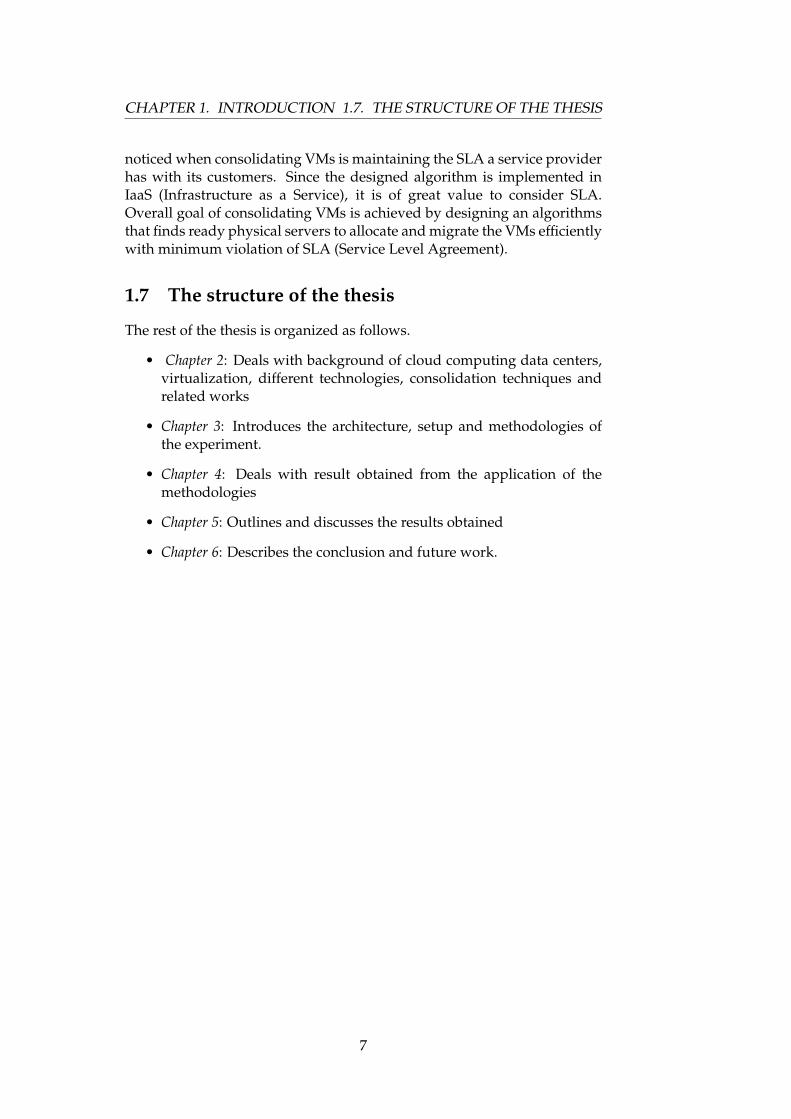
4.2.3 Stochastic approach I VM location
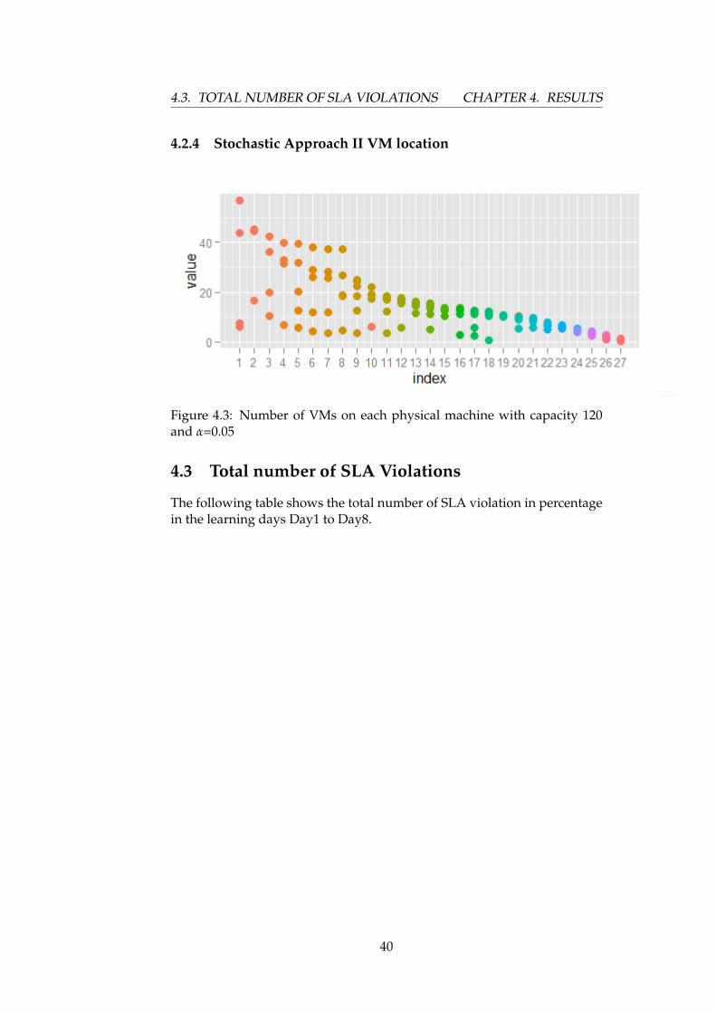
Figure 4.2: Number of VMs on each physical machine with capacity 120and α=0.05
39
4.3. TOTAL NUMBER OF SLA VIOLATIONS CHAPTER 4. RESULTS
4.2.4 Stochastic Approach II VM location
Figure 4.3: Number of VMs on each physical machine with capacity 120and α=0.05
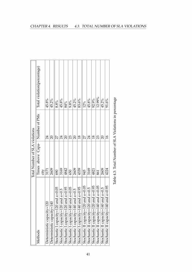
4.3 Total number of SLA Violations
The following table shows the total number of SLA violation in percentagein the learning days Day1 to Day8.
40
CHAPTER 4. RESULTS 4.3. TOTAL NUMBER OF SLA VIOLATIONS
Tota
lNum
ber
ofSL
Avi
olat
ions
Met
hods
Tim
esab
ove
Cap
a-ci
tyN
umbe
rof
PMs
Tota
lvio
lati
on(p
erce
ntag
e)
Det
erm
inis
tic
capa
city
=120
3171
2445
.8%
Det
erm
inis
tic
capa
city
=140
2609
2045
.2%
Stoc
hast
icIc
apac
ity=
120
and
α=0
.05
690
278.
8%St
ocha
stic
Icap
acit
y=12
0an
dα
=0.5
3169
2445
.8%
Stoc
hast
icIc
apac
ity=
120
and
α=0
.95
4842
2084
%St
ocha
stic
Icap
acit
y=14
0an
dα
=0.0
565
023
9.8%
Stoc
hast
icIc
apac
ity=
140
and
α=0
.526
0920
45.2
%St
ocha
stic
Icap
acit
y=14
0an
dα
=0.9
543
3918
83.6
%St
ocha
stic
IIca
paci
ty=1
20an
dα
=0.0
594
527
12%
Stoc
hast
icII
capa
city
=120
and
α=0
.531
6924
45.8
%St
ocha
stic
IIca
paci
ty=1
20an
dα
=0.9
548
2118
92.9
%St
ocha
stic
IIca
paci
ty=1
40an
dα
=0.0
586
123
12.9
9%St
ocha
stic
IIca
paci
ty=1
40an
dα
=0.5
2609
2045
.2%
Stoc
hast
icII
capa
city
=140
and
α=0
.95
4224
1691
.6%
Tabl
e4.
3:To
talN
umbe
rof
SLA
Vio
lati
ons
inpe
rcen
tage
41
4.4. DESCRIPTION OF RESULTS CHAPTER 4. RESULTS
4.4 Description of Results
4.4.1 Observation on PMs utilization
As it can be seen from Table 4.1 and Table 4.2, though the thresholdscenarios are the same, one can easily observe the following differences:-
• The number of PM used to accommodate the VMs in the data setshows significant differences.
• Deterministic approach with capacity 120 uses equal number of PMswith stochastic approach I with α = 0.5. Similar observation are seenbetween deterministic approach with capacity 140 and stochasticapproach with α = 0.95 .
• Types of VMs,i.e VM with average CPU load, on each PM aredifferent for all approaches see Appendix F.
• Similar differences among the approaches and scenarios are observedon the graphs and tables.
Generally, in Table 4.1 and 4.2, stochastic approach I and II withcapacity 120 and α = 0.05 appears to use the maximum number of PMsto consolidate the VMs in the data set. Contrarily, the same approacheswith capacity 120 and α = 0.95 utilized the minimum number of VMs,i.e 20 and 18 respectively, to home the VMs.The deterministic approach inthis regard shows neither maximum nor minimum utilization of the PMs.As α increases, naturally we can place more VMs on each PM. This is inaccordance with table 4.2 and 4.3.
When the capacity for all approaches become 140, deterministicapproach uses 20 and the stochastic approach I and II with α = 0.05 usesthe maximum number of PMs, i.e 23, to home the VMs. On the other side,stochastic approach I and II with α = 0.95 used 18 and 16 PMs respectively.Again, the deterministic approach shows neither maximum nor minimumutilization of PMs with the capacity under discussion. Thus, it is observedthat as α increases, more VMs can be place on the PM and the number ofPM utilized decreases for capacity 140 too.
42
CHAPTER 4. RESULTS 4.4. DESCRIPTION OF RESULTS
Observation on number of VMs on each PM
As it can be seen from the above figures, in Figure 4.1 the first and secondPMs homed 3 VMs and the third PM has 4 VMs in deterministic approach.For stochastic approach I, figure 4.2 shows that the first, second and thirdPMs accomodated 3 VMs each and the fourth PM has 4 VMs on it. Furthermore, as Figure 4.3 shows using stochastic approach II the first PM homed4 VMs and the second and third has 3 VMs each and so on. Theseshows that the capacity of the same VMs are welcomed differently fordifferent approaches. The average CPU load of each VM is different inboth scenarios(capacity 120 and 140). Thus, the capacity of the PM mattersat-least to hold the type of VMs even though it is insignificant, and this inturn affects over all operational cost of the data center. For the rest of theresult see Appendix F
4.4.2 Observation on SLA violation
Table 4.3 shows the total number of SLA violation incurred in eachapproach. The maximum number of SLA violation incurred was bystochastic approach II with capacity 120 and α = 0.95 which is ca. 92.9%followed by the same approach with capacity 140 and α = 0.95(91.6%).
When capacity is 120 for all approaches the maximum SLA violationwas done by stochastic approach II with α = 0.95 and the minimum wasdone by stochastic approach I with α = 0.05 which is ca. 8.8%.
when capacity is 140 for all approaches the maximum SLA violationoccurred was by stochastic approach II with α = 0.95 which is 91.6% andthe minimum violation was seen in stochastic approach I with α = 0.05which is 9.8%
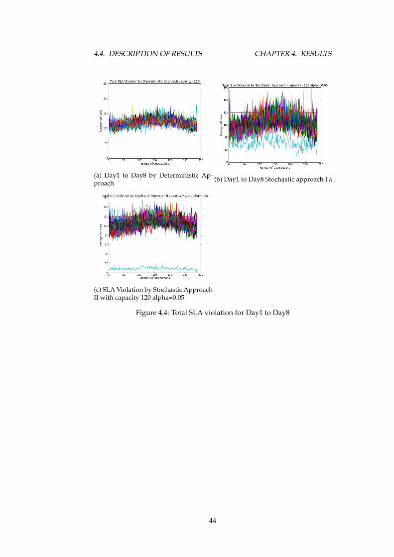
The following graph, Figure 4.15 (a), (b), and (c) show the total violationof SLA in graphs by the three approaches: deterministic, stochastic I, andstochastic II, for Day1 to Day8 with capacity 120 respectively.
From Figure 4.15 and Figure 4.16, one can conclude that the trend ofviolating SLA shows the same pattern in both learning days (Day1 to Day8)and evaluation days (Day9 and Day10). This is because of the average ofaggregate load values we use to compute load for VMs in different days forprovisioning.
43
4.4. DESCRIPTION OF RESULTS CHAPTER 4. RESULTS
(a) Day1 to Day8 by Deterministic Ap-proach (b) Day1 to Day8 Stochastic approach I α
(c) SLA Violation by Stochastic ApproachII with capacity 120 alpha=0.05
Figure 4.4: Total SLA violation for Day1 to Day8
44
CHAPTER 4. RESULTS 4.5. EVALUATION DAYS RESULT
4.5 Evaluation Days Result
4.5.1 Number of utilized PMs
Number of of used PMs, Deterministic Approach for Day9Methods Capacity=120 Capacity=140mean 24 20
Table 4.4: Number of PMs used by Deterministic approach for Day9 andDay10
Day9—————————– Capacity = 120—–| ————-capacity =140Methods α =0.05 α =0.5 α =0.95 α =0.05 α =0.5 α =0.95Variance 27 24 20 23 20 7Covariance 27 24 20 23 20 8
Table 4.5: Number of PMs used by Stochastic Approach I and II for day9and day10
4.5.2 Total number of SLA violations
The following table shows the total number of SLA violation in percentageover evaluation days.
45
4.5. EVALUATION DAYS RESULT CHAPTER 4. RESULTS
Tota
lNum
ber
ofSL
Avi
olat
ions
Met
hods
Tim
esab
ove
Cap
acit
yN
umbe
rof
PMs
Tota
lvio
lati
on(p
erce
ntag
e)D
eter
min
isti
cca
paci
ty=1
2031
7324
45.8
%D
eter
min
isti
cca
paci
ty=1
4026
0920
45.2
%St
ocha
stic
Icap
acit
y=12
0an
dα
=0.0
575
027
9.6%
Stoc
hast
icIc
apac
ity=
120
and
α=0
.531
6924
45.8
%St
ocha
stic
Icap
acit
y=12
0an
dα
=0.9
547
6420
82.7
%St
ocha
stic
Icap
acit
y=14
0an
dα
=0.0
570
823
10.6
%St
ocha
stic
Icap
acit
y=14
0an
dα
=0.5
2609
2048
.2%
Stoc
hast
icIc
apac
ity=
140
and
α=0
.95
4293
1882
.8%
Stoc
hast
icII
capa
city
=120
and
α=0
.05
758
2725
.3%
Stoc
hast
icII
capa
city
=120
and
α=0
.531
6920
45.8
%St
ocha
stic
IIca
paci
ty=1
20an
dα
=0.9
548
4218
84%
Stoc
hast
icII
capa
city
=140
and
α=0
.05
650
239.
8%St
ocha
stic
IIca
paci
ty=1
40an
dα
=0.5
2609
2045
.2%
Stoc
hast
icII
capa
city
=140
and
α=0
.95
4866
1893
.8%
Tabl
e4.
6:To
talN
umbe
rof
SLA
Vio
lati
ons
inpe
rcen
tage
inD
ay9
and
Day
10
46
CHAPTER 4. RESULTS4.6. DESCRIPTION OF EVALUATION DAYS RESULT
4.6 Description of Evaluation Days Result
4.6.1 Observation on PM utilization
Deterministic Approach
The above tables, Table 4.5 and Table 4.6, show that the number of PMsutilized tend to go with the capacity. 24 PMs were used and 20 PMs withcapacity 140 to consolidate VMs. This shows that number of PMs useddecreases with increased capacity.
Stochastic Approach I and II
In both approaches, it shows that when capacity increase the number ofPMs used decreases. But as α increases, both approaches show decrease inutilization of PMs. Special figure that is observed in the table is that, thestochastic approach I and stochastic approach II gives equal value in all thethreshold values, α.
4.6.2 Observation on SLA violation
In deterministic approach total percentage violation of SLA seems to beconstant or similar with increased capacity as observed from Table 4.6, butin stochastic approaches, it can be concluded that total percentage of SLAviolation increases as α increases. In addition, stochastic approach II tendsto use less PMs when α=0.95 in both capacities. For α=0.5 we observe nodifference between the three approaches in violating total percentage ofSLA.
Generally, it is observed that the number of PMs used are equal inall approaches when α=0.5. Furthermore, stochastic approach II tendsto use minimum number of PMs and stochastic approach I and II showthe maximum number of PM utilization. Moreover, stochastic approachI shows minimum total percentage of SLA violation and stochasticapproach II showed maximum total percentage of SLA violation. In allcases, deterministic approach showed average in total percentage of SLAviolation. Number of times above provisioned capacity increases withdecrease in α, which is very natural, but in case of deterministic approachthe result showed the opposite because of increase in capacity. Thus, whenwe compare Table 4.6 with Table 4.3 they follow the same pattern both inutilizing PMs and in total percentage of SLA violation.
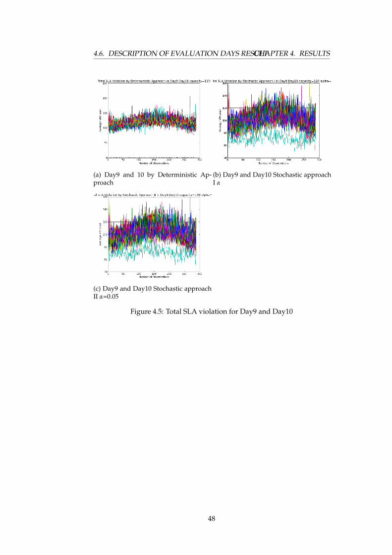
The following graph shows the total percentage of SLA violation by thethree approaches with capacity 120. As depicted earlier, the graph followsthe same pattern with that of learning days graph, Figure 4.15.
47
4.6. DESCRIPTION OF EVALUATION DAYS RESULTCHAPTER 4. RESULTS
(a) Day9 and 10 by Deterministic Ap-proach
(b) Day9 and Day10 Stochastic approachI α
(c) Day9 and Day10 Stochastic approachII α=0.05
Figure 4.5: Total SLA violation for Day9 and Day10
48
CHAPTER 4. RESULTS4.7. COVARIANCE AND CORRELATION MATRIX RESULT
4.7 Covariance and Correlation matrix Result
Covariance and Correlation matrix for the VMs in the selected data set fromall days is shown in Figure 4.6 and 4.7 respectively. This is just to show theditribution of the data set. As it can be seen from Figure 4.6 below, thereare very few observation with high-covariance.
Figure 4.6: Covariance among the data-set
The correlation between pair of VMs in a data-set with time-stamp(x1, x2, x3, ..., xn and y1, y2, y3, ..., ynwere computed using PearsonCorrelation Coefficient.
ρxy =COVxy
sdx ∗ sdy(4.2)
where, sdx and sdy are standard deviation of x and yFigure 4.7 shows that there are few VMs with both positively correlated
and negatively correlated.
49

4.7. COVARIANCE AND CORRELATION MATRIX RESULTCHAPTER 4. RESULTS
Figure 4.7: Correlation among the data-set
50

CHAPTER 4. RESULTS4.7. COVARIANCE AND CORRELATION MATRIX RESULT
51
4.7. COVARIANCE AND CORRELATION MATRIX RESULTCHAPTER 4. RESULTS
52
Chapter 5
Discussion
In this chapter, discussion and analysis of the results obtained will bepresented in detail.
The goal of this paper is to explore and see how to reduce operationalcost of a data center by consolidating VMs. The main target of consolid-ating VMs is to optimize the efficiency of resource utilization in the datacenter. Efficiently optimization of resources include the reduction of PMutilizatioin and SLA violation during consolidation. Thus, this paper fo-cuses mainly on reducing the operational cost in light of reducing the totalnumber of PMs used and the total number of SLA violations.
Several researches has been conducted on the subject of consolidatingVMs in a data center to reduce the total operational cost. By reviewingrelated researches, we end up in designing our own algorithm to tacklethe problems of a data center. In order to achieve this we first found waysof how to detect the overloading status of a PM. Secondly, techniques tomigrate VMs from the overloaded hosts are selected. Thus, mean, varianceand covariance were used to determine if the hosts are overloaded ornot. Furthermore, first fit decreasing bin-packing technique was selectedas mechanism to migrate VMs . Based on these three approaches, analgorithm was designed to conduct simulation of consolidating the VMsfor our data set.
Results from the experiment of the simulation show that the determin-istic approach showed similar results for violation of SLA both in learningdays and evaluation days. In both cases, the only difference seen was onthe number of PMs utilized when capacity changes. This by itself is veryinsignificant in reducing the SLA violation, though it showed positive ef-fect. The same analysis holds true for the stochastic approaches, but withslight difference in percentage of SLA violation.
In stochastic approaches, increase in percentage of SLA violation goeswith increase in α. But the number of PM utilization goes up inversely withα, that means when we increase α, minimum number of PMs are used.Though increasing the capacity of a PM helps in reducing the number ofPMs used, it shows very little difference on SLA violation both in stochasticapproach I and II. SLA violation increases with decrease in capacity in bothdeterministic and stochastic approaches.
53
CHAPTER 5. DISCUSSION
As depicted on Table 4.3 in previous chapter, the same number of PMsare used by different approaches, for example deterministic approach withcapacity 120 and stochastic approach with capacity 120 and α=0.5, usethe same number of PMs and also the same percentage in SLA violation.Simultaneously, Table 4.6 shows the same result for deterministic approachand stochastic approach I and II with α=0.5.
Following that, we conclude that the effect of using covariance(stochastic approach II) in our case, for the selected data set is very low.This can be the result of too little dependencies between VM’s real data.
There are different factors that can reduce the occurrence of SLAviolation. Some of them are, limiting the provisioned capacity, whichresults in increasing the number of PMs and decreasing the number orpercentage of SLA violation. For instance, we experimented this byprovision only 90% of the capacity of the PM available. The followingTable5.1 shows the result.
Total Number of SLA violations with 90 percent of the CapacityMethods Times above Ca-
pacityNumber of PMs violation (per-
centage)Deterministic capa-city=120
1274 26 17%
Deterministic capa-city=140
1044 22 16.4%
Stochastic I capa-city=120 and α=0.05
114 30 1.3%
Stochastic I capa-city=140 and α=0.05
1373 26 18.8%
Stochastic II capa-city=120 and α=0.05
141 30 1.63%
Stochastic II capa-city=140 and α=0.05
1717 25 23.8%
Table 5.1: Total Number of SLA Violations after introduction of 90% ofcapacity
Thus, comparing the above Table 5.1 with Table 4.3 of previous chapterit can be concluded that if threshold is set to a provisioned capacity, itwill end up in decreasing number of SLA violation by 83%, sacrificingadditional 11% of the existing PMs.
In order to test the efficiency of the designed algorithm, the same dataset of VMs are extracted from Day9 and Day10 of our obtained data. Then,the algorithm yielded the result on Table 4.6 that are found in previouschapter. The results depict that changing capacity have brought change inutilization of number of physical machines in deterministic approach, butshowed almost no change in percentage violation of SLA the result as thatof our learning days. In the other two approaches, stochastic approach Iand II, total percentage of SLA violation increases with α. But, when we
54
CHAPTER 5. DISCUSSION 5.1. SUMMARY
look at total percentage of SLA violation as we increase capacity, it showsalmost no change for α=0.5 similar to that of deterministic approach. Thesame analysis holds true for stochastic approach II. In general percentageof SLA violation goes inversely with capacity. Thus increased percentageof SLA violation shows decrease in number of PMs or vice versa.
5.1 Summary
From the experiment it is observed that there are trade-off betweenmaintaining SLA and utilization of PM. The three approaches we selectedalso have shown different results leading us to conclude that one ofthe most challenging task in consolidating VMs is designing a systemthat balances between PM utilization and SLA. Thus, out of the threeapproaches implemented, it is observed that consolidation by stochasticapproach II used minimum PM in both capacities and stochastic approachI showed minimum percentage of SLA violation in both capacities forVMs in learning days. Furthermore, it is observed that consolidation bystochastic approach I uses minimum PM in both capacities and at the sametime have minimum percentage of SLA violation in both capacities for theevaluation days. Moreover, both learning days and evaluation days tendto use the same number of PMs in almost all of the approaches, except onthe stochastic approach II with α=0.95. Thus, stochastic approach I willbe selected for its minimum violation of SLA and stochastic approach II isselected for usage of minimum number of PMs.
55

5.1. SUMMARY CHAPTER 5. DISCUSSION
56
Chapter 6
Conclusion and Future work
In cloud data centers one of the main goal of consolidating VMs is tooptimize the efficiency of resource utilization and maintain SLA(servicelevel agreement). One of the challenging tasks of cloud service providersis to provision required resources and at the same time keep SLA. In thispaper, we experimented and presented three approaches to consolidateVMs with the aim of reducing the overall operational cost of a data centerby minimizing the use of PMs and percentage of SLA violation. In orderto do this, simulation on real-workload traces obtained from PlanetLabWorkload-traces which was logged randomly every 5 minutes for 10 daysin 2011 were selected. From the obtained data, VMs that have highobservations in the learning days (Day1 to Day8) are selected as our targetdata set. Based on this analysis, a script that captures the workload of theVMs in a data set was developed. Besides, four similar but different scriptswere developed to apply heuristic bin-packing script for deterministicapproach, stochastic approach I and II, and SLA violation counter andplotter respectively (see the Appendix A, B, C, D and E for more).
The three approaches introduced have shown different results. Basedon their results, we concluded that stochastic approach I withα=0.05 haveshown good result for consolidating the VMs in our data set. Thus, wepropose stochastic approach I approach for consolidation of VMs withminimum violation of SLA in both learning days and evaluation days.Stochastic approach II will be selected for minimum utilization of PMs forboth learning days and evaluation days.
In all approaches, the results show that there are trade-off betweenpercentage of SLA violation and utilization of PMs. It is already mentionedin earlier chapter that our system architecture is designed for IaaS(Infrastructure as a Service) which could be implemented for cloud serviceproviders like open stack. Though the scope of this thesis is not up to thatlevel, we propose that tailoring the problem between the service providerand consumer could be of reconciling solution when provisioning VMs.This assumption is based on the result we get from Table 5.1 of discussionchapter. The goal of this paper is exploring how to reduce the operationalcost of a data center by consolidating VMs. One of the benefits of this workis reducing the number of used PMs and also minimize the total percentage
57
CHAPTER 6. CONCLUSION AND FUTURE WORK
of SLA violation. Which in turn reduces the overall operational cost ofa data center. From the experiment we discovered that it is difficult toguarantee 100% SLA in consolidation. But, further studies may result inmore minimized SLA violation than we proposed.
Additional goal that can be pursued with the proposed methodologiesmentioned is reduction of power consumption. Cost of power consump-tion in a data center is directly affected by number of physical machinesutilized. This is because of linear relationship between CPU utilization andpower consumption. Thus, we believe that we save cost of power con-sumption with the proposed methodologies, but incorporating calculationof power consumption could be one of the future works of such project.Furthermore, as mentioned earlier this work focused mainly only on theCPU utilization of VMs and the other constraints such as memory andbandwidth utilization are not included. Thus, incorporating them will beadditional future work for such kind of project.
58

CHAPTER 6. CONCLUSION AND FUTURE WORK
59
CHAPTER 6. CONCLUSION AND FUTURE WORK
60
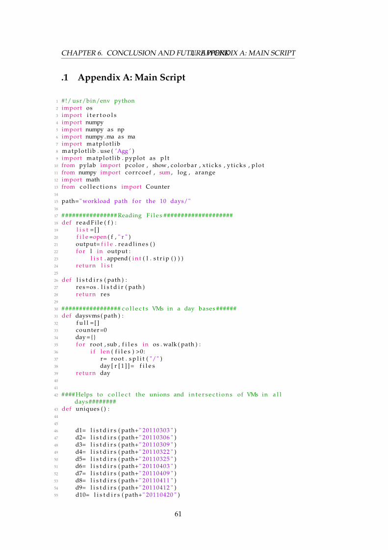
CHAPTER 6. CONCLUSION AND FUTURE WORK.1. APPENDIX A: MAIN SCRIPT
.1 Appendix A: Main Script
1 # !/ usr/bin/env python2 import os3 import i t e r t o o l s4 import numpy5 import numpy as np6 import numpy .ma as ma7 import m a t p l o t l i b8 m a t p l o t l i b . use ( ’Agg ’ )9 import m a t p l o t l i b . pyplot as p l t
10 from pylab import pcolor , show , colorbar , x t i c k s , y t i c ks , p l o t11 from numpy import corrcoef , sum , log , arange12 import math13 from c o l l e c t i o n s import Counter14
15 path=" workload path f o r the 10 days/"16
17 # ############### Reading F i l e s ####################18 def r e a d F i l e ( f ) :19 l i s t = [ ]20 f i l e =open ( f , " r " )21 output= f i l e . r e a d l i n e s ( )22 f o r l in output :23 l i s t . append ( i n t ( l . s t r i p ( ) ) )24 re turn l i s t25
26 def l i s t d i r s ( path ) :27 re s=os . l i s t d i r ( path )28 re turn r es29
30 # ################ c o l l e c t s VMs in a day bases ######31 def daysvms ( path ) :32 f u l l = [ ]33 counter =034 day = { }35 f o r root , sub , f i l e s in os . walk ( path ) :36 i f len ( f i l e s ) >0:37 r= root . s p l i t ( "/" )38 day [ r [ 1 ] ] = f i l e s39 re turn day40
41
42 #### Helps to c o l l e c t the unions and i n t e r s e c t i o n s of VMs in a l ldays ########
43 def uniques ( ) :44
45
46 d1= l i s t d i r s ( path+" 20110303 " )47 d2= l i s t d i r s ( path+" 20110306 " )48 d3= l i s t d i r s ( path+" 20110309 " )49 d4= l i s t d i r s ( path+" 20110322 " )50 d5= l i s t d i r s ( path+" 20110325 " )51 d6= l i s t d i r s ( path+" 20110403 " )52 d7= l i s t d i r s ( path+" 20110409 " )53 d8= l i s t d i r s ( path+" 20110411 " )54 d9= l i s t d i r s ( path+" 20110412 " )55 d10= l i s t d i r s ( path+" 20110420 " )
61
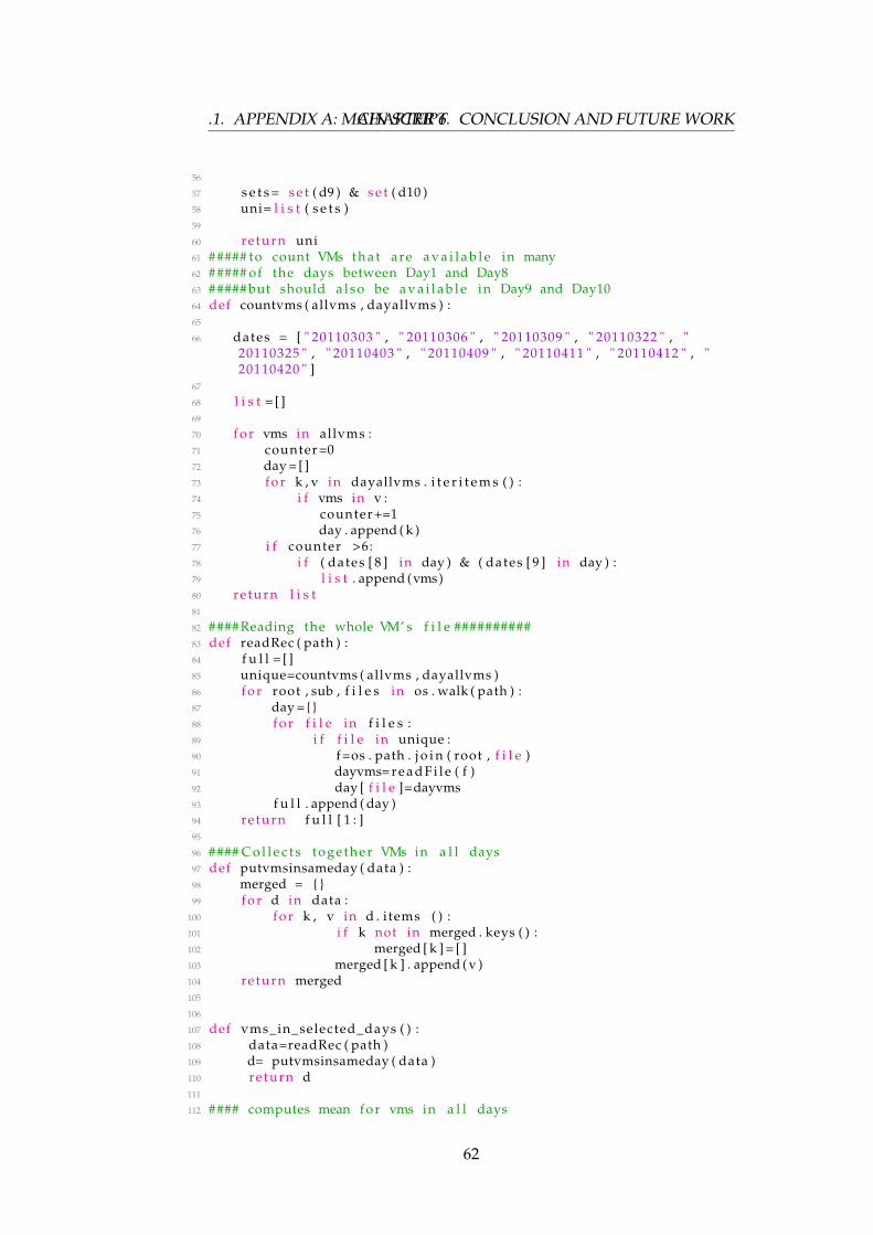
.1. APPENDIX A: MAIN SCRIPTCHAPTER 6. CONCLUSION AND FUTURE WORK
56
57 s e t s = s e t ( d9 ) & s e t ( d10 )58 uni= l i s t ( s e t s )59
60 re turn uni61 # #### to count VMs t h a t are a v a i l a b l e in many62 # #### of the days between Day1 and Day863 # #### but should a l s o be a v a i l a b l e in Day9 and Day1064 def countvms ( allvms , dayallvms ) :65
66 dates = [ " 20110303 " , " 20110306 " , " 20110309 " , " 20110322 " , "20110325 " , " 20110403 " , " 20110409 " , " 20110411 " , " 20110412 " , "20110420 " ]
67
68 l i s t = [ ]69
70 f o r vms in allvms :71 counter =072 day = [ ]73 f o r k , v in dayallvms . i t e r i t e m s ( ) :74 i f vms in v :75 counter+=176 day . append ( k )77 i f counter >6:78 i f ( dates [ 8 ] in day ) & ( dates [ 9 ] in day ) :79 l i s t . append (vms)80 re turn l i s t81
82 #### Reading the whole VM’ s f i l e ##########83 def readRec ( path ) :84 f u l l = [ ]85 unique=countvms ( allvms , dayallvms )86 f o r root , sub , f i l e s in os . walk ( path ) :87 day = { }88 f o r f i l e in f i l e s :89 i f f i l e in unique :90 f =os . path . j o i n ( root , f i l e )91 dayvms= r e a d F i l e ( f )92 day [ f i l e ]=dayvms93 f u l l . append ( day )94 re turn f u l l [ 1 : ]95
96 #### C o l l e c t s toge ther VMs in a l l days97 def putvmsinsameday ( data ) :98 merged = { }99 f o r d in data :
100 f o r k , v in d . items ( ) :101 i f k not in merged . keys ( ) :102 merged [ k ] = [ ]103 merged [ k ] . append ( v )104 re turn merged105
106
107 def vms_in_selected_days ( ) :108 data=readRec ( path )109 d= putvmsinsameday ( data )110 re turn d111
112 #### computes mean f o r vms in a l l days
62
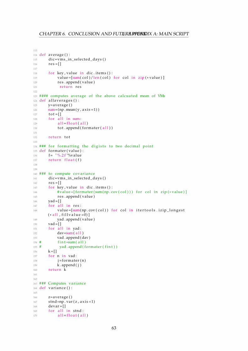
CHAPTER 6. CONCLUSION AND FUTURE WORK.1. APPENDIX A: MAIN SCRIPT
113
114 def average ( ) :115 dic=vms_in_selected_days ( )116 re s = [ ]117
118 f o r key , value in dic . i tems ( ) :119 value =[sum( c o l ) /len ( c o l ) f o r c o l in zip ( * value ) ]120 r es . append ( value )121 re turn r es122
123 #### computes average of the above ca lcuated mean of VMs124 def a l l a v e r a g e s ( ) :125 y=average ( )126 sum=(np . mean( y , a x i s =1) )127 t o t = [ ]128 f o r a l l in sum :129 a l l = f l o a t ( a l l )130 t o t . append ( formater ( a l l ) )131
132 re turn t o t133
134 ### f o r formatt ing the d i g i s t s to two decimal point135 def formater ( value ) :136 f = " %.2 f "%value137 re turn f l o a t ( f )138
139
140 ### to compute covar iance141 dic=vms_in_selected_days ( )142 re s = [ ]143 f o r key , value in dic . i tems ( ) :144 # value =[ formater (sum( np . cov ( c o l ) ) ) f o r c o l in zip ( * value ) ]145 r es . append ( value )146 yad = [ ]147 f o r a l l in r es :148 value =[sum( np . cov ( c o l ) ) f o r c o l in i t e r t o o l s . i z i p _ l o n g e s t
( * a l l , f i l l v a l u e =0) ]149 yad . append ( value )150 vad = [ ]151 f o r a l l in yad :152 dav=sum( a l l )153 vad . append ( dav )154 # f i n t =sum( a l l )155 # yad . append ( formater ( f i n t ) )156 k = [ ]157 f o r n in vad :158 j =formater ( n )159 k . append ( j )160 re turn k161
162
163 ### Computes var iance164 def var iance ( ) :165
166 z=average ( )167 stnd=np . var ( z , a x i s =1)168 devar = [ ]169 f o r a l l in stnd :170 a l l = f l o a t ( a l l )
63
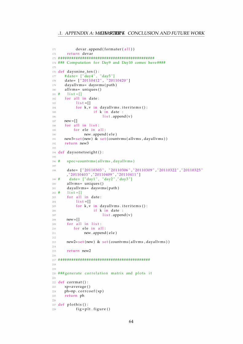
.1. APPENDIX A: MAIN SCRIPTCHAPTER 6. CONCLUSION AND FUTURE WORK
171 devar . append ( formater ( a l l ) )172 re turn devar173 # ###########################################174 ### Computation f o r Day9 and Day10 comes here ####175
176 def daysnine_ten ( ) :177 # date= [ " day4 " , " day5 " ]178 date= [ " 20110412 " , " 20110420 " ]179 dayallvms= daysvms ( path )180 allvms= uniques ( )181 # l i s t = [ ]182 f o r a l l in date :183 l i s t = [ ]184 f o r k , v in dayallvms . i t e r i t e m s ( ) :185 i f k in date :186 l i s t . append ( v )187 new= [ ]188 f o r a l l in l i s t :189 f o r e l e in a l l :190 new . append ( e l e )191 new3= s e t (new) & s e t ( countvms ( allvms , dayallvms ) )192 re turn new3193
194 def daysonetoeight ( ) :195
196 # spec=countvms ( allvms , dayallvms )197
198 date= [ " 20110303 " , " 20110306 " , " 20110309 " , " 20110322 " , " 20110325 ", " 20110403 " , " 20110409 " , " 20110411 " ]
199 # date= [ " day1 " , " day2 " , " day3 " ]200 allvms= uniques ( )201 dayallvms= daysvms ( path )202 # l i s t = [ ]203 f o r a l l in date :204 l i s t = [ ]205 f o r k , v in dayallvms . i t e r i t e m s ( ) :206 i f k in date :207 l i s t . append ( v )208 new= [ ]209 f o r a l l in l i s t :210 f o r e l e in a l l :211 new . append ( e l e )212
213 new2= s e t (new) & s e t ( countvms ( allvms , dayallvms ) )214
215 re turn new2216
217 # #########################################218
219
220 ### generate c o r r e l a t i o n matrix and p l o t s i t221
222 def corrmat ( ) :223 xp=average ( )224 ph=np . c o r r c o e f ( xp )225 re turn ph226
227 def p l o t h i s ( ) :228 f i g = p l t . f i g u r e ( )
64
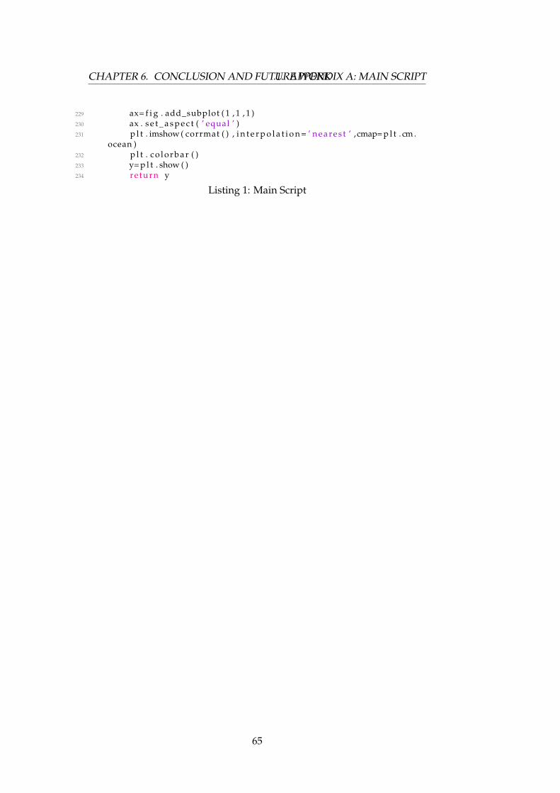
CHAPTER 6. CONCLUSION AND FUTURE WORK.1. APPENDIX A: MAIN SCRIPT
229 ax= f i g . add_subplot ( 1 , 1 , 1 )230 ax . s e t _ a s p e c t ( ’ equal ’ )231 p l t . imshow ( corrmat ( ) , i n t e r p o l a t i o n = ’ n e a r e s t ’ , cmap= p l t . cm .
ocean )232 p l t . c o l or ba r ( )233 y= p l t . show ( )234 re turn y
Listing 1: Main Script
65
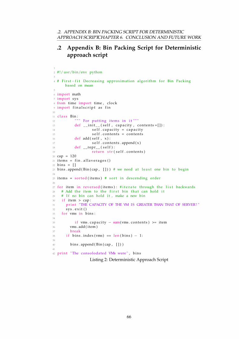
.2. APPENDIX B: BIN PACKING SCRIPT FOR DETERMINISTICAPPROACH SCRIPTCHAPTER 6. CONCLUSION AND FUTURE WORK
.2 Appendix B: Bin Packing Script for Deterministicapproach script
1
2 # !/ usr/bin/env python3
4 # F i r s t− f i t Decreasing approximation algorithm f o r Bin Packingbased on mean
5
6 import math7 import sys8 from time import time , c lock9 import f i n a l s c r i p t as f i n
10
11 c l a s s Bin :12 " " " For putt ing items in i t " " "13 def _ _ i n i t _ _ ( s e l f , capaci ty , contents = [ ] ) :14 s e l f . c a p a c i t y = c a p a c i t y15 s e l f . contents = contents16 def add ( s e l f , x ) :17 s e l f . contents . append ( x )18 def __repr__ ( s e l f ) :19 re turn s t r ( s e l f . contents )20 cap = 12021 i tems = f i n . a l l a v e r a g e s ( )22 bins = [ ]23 bins . append ( Bin ( cap , [ ] ) ) # we need at l e a s t one bin to begin24
25 i tems = sorted ( items ) # s o r t in descending order26
27 f o r item in reversed ( items ) : # i t e r a t e through the l i s t backwards28 # Add the item to the f i r s t bin t h a t can hold i t29 # I f no bin can hold i t , make a new bin30 i f item > cap :31 p r i n t "THE CAPACITY OF THE VM IS GREATER THAN THAT OF SERVER ! "32 sys . e x i t ( )33 f o r vms in bins :34
35 i f vms . c a p a c i t y − sum(vms . contents ) >= item36 vms . add ( item )37 break38 i f b ins . index (vms) == len ( bins ) − 1 :39
40 bins . append ( Bin ( cap , [ ] ) )41
42 p r i n t " The consolodated VMs were " , bins
Listing 2: Deterministic Approach Script
66
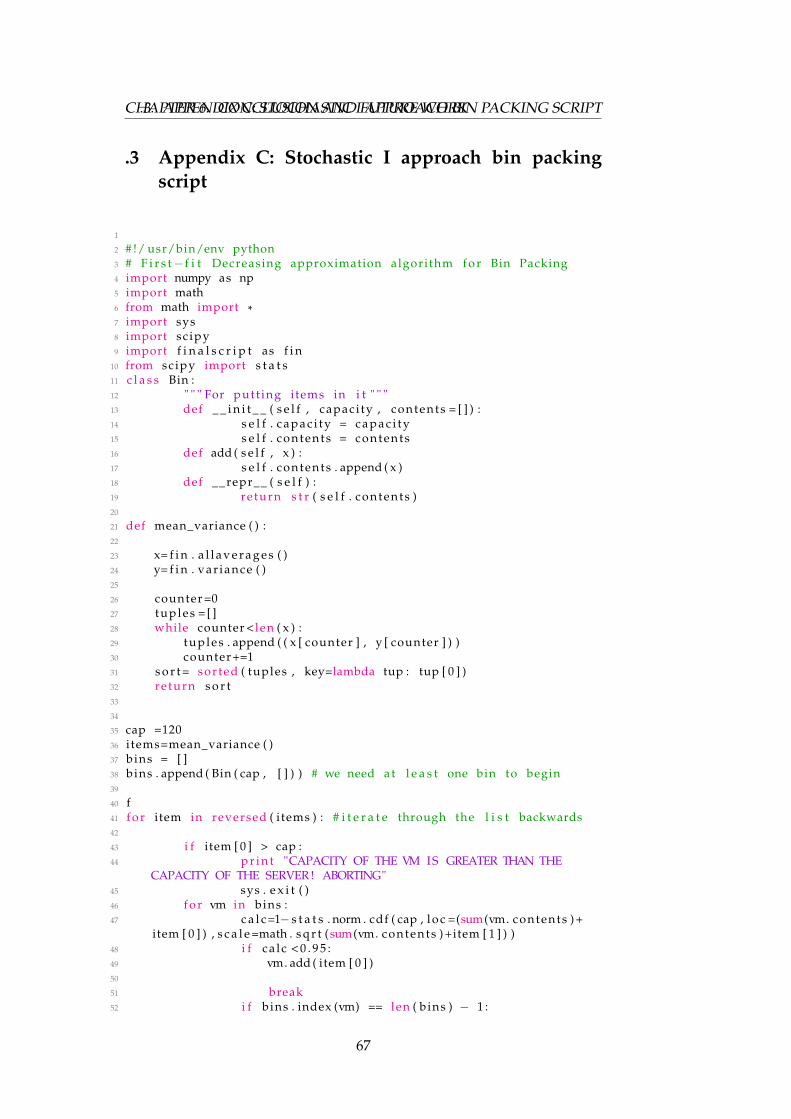
CHAPTER 6. CONCLUSION AND FUTURE WORK.3. APPENDIX C: STOCHASTIC I APPROACH BIN PACKING SCRIPT
.3 Appendix C: Stochastic I approach bin packingscript
1
2 # !/ usr/bin/env python3 # F i r s t− f i t Decreasing approximation algorithm f o r Bin Packing4 import numpy as np5 import math6 from math import *7 import sys8 import sc ipy9 import f i n a l s c r i p t as f i n
10 from scipy import s t a t s11 c l a s s Bin :12 " " " For putt ing items in i t " " "13 def _ _ i n i t _ _ ( s e l f , capaci ty , contents = [ ] ) :14 s e l f . c a p a c i t y = c a p a c i t y15 s e l f . contents = contents16 def add ( s e l f , x ) :17 s e l f . contents . append ( x )18 def __repr__ ( s e l f ) :19 re turn s t r ( s e l f . contents )20
21 def mean_variance ( ) :22
23 x= f i n . a l l a v e r a g e s ( )24 y= f i n . var iance ( )25
26 counter =027 tup l es = [ ]28 while counter <len ( x ) :29 tup l es . append ( ( x [ counter ] , y [ counter ] ) )30 counter+=131 s o r t = sor ted ( tuples , key=lambda tup : tup [ 0 ] )32 re turn s o r t33
34
35 cap =12036 i tems=mean_variance ( )37 bins = [ ]38 bins . append ( Bin ( cap , [ ] ) ) # we need at l e a s t one bin to begin39
40 f41 f o r item in reversed ( items ) : # i t e r a t e through the l i s t backwards42
43 i f item [ 0 ] > cap :44 p r i n t "CAPACITY OF THE VM IS GREATER THAN THE
CAPACITY OF THE SERVER ! ABORTING"45 sys . e x i t ( )46 f o r vm in bins :47 c a l c=1− s t a t s . norm . cdf ( cap , l o c =(sum(vm. contents ) +
item [ 0 ] ) , s c a l e =math . s q r t (sum(vm. contents ) +item [ 1 ] ) )48 i f ca lc < 0 . 9 5 :49 vm. add ( item [ 0 ] )50
51 break52 i f b ins . index (vm) == len ( bins ) − 1 :
67

.3. APPENDIX C: STOCHASTIC I APPROACH BIN PACKING SCRIPTCHAPTER 6. CONCLUSION AND FUTURE WORK
53
54 bins . append ( Bin ( cap , [ ] ) )55
56
57 p r i n t "\n\nThe c o n s o l i d a t i o n i s as fo l lows :\n\n" , bins58
59
60
Listing 3: Stochastic I script
68
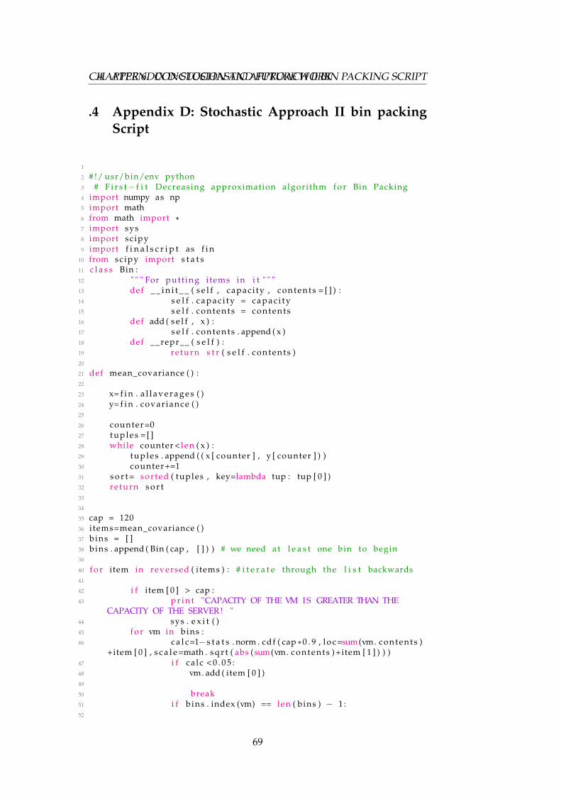
CHAPTER 6. CONCLUSION AND FUTURE WORK.4. APPENDIX D: STOCHASTIC APPROACH II BIN PACKING SCRIPT
.4 Appendix D: Stochastic Approach II bin packingScript
1
2 # !/ usr/bin/env python3 # F i r s t− f i t Decreasing approximation algorithm f o r Bin Packing4 import numpy as np5 import math6 from math import *7 import sys8 import sc ipy9 import f i n a l s c r i p t as f i n
10 from scipy import s t a t s11 c l a s s Bin :12 " " " For putt ing items in i t " " "13 def _ _ i n i t _ _ ( s e l f , capaci ty , contents = [ ] ) :14 s e l f . c a p a c i t y = c a p a c i t y15 s e l f . contents = contents16 def add ( s e l f , x ) :17 s e l f . contents . append ( x )18 def __repr__ ( s e l f ) :19 re turn s t r ( s e l f . contents )20
21 def mean_covariance ( ) :22
23 x= f i n . a l l a v e r a g e s ( )24 y= f i n . covar iance ( )25
26 counter =027 tup l es = [ ]28 while counter <len ( x ) :29 tup l es . append ( ( x [ counter ] , y [ counter ] ) )30 counter+=131 s o r t = sor ted ( tuples , key=lambda tup : tup [ 0 ] )32 re turn s o r t33
34
35 cap = 12036 i tems=mean_covariance ( )37 bins = [ ]38 bins . append ( Bin ( cap , [ ] ) ) # we need at l e a s t one bin to begin39
40 f o r item in reversed ( items ) : # i t e r a t e through the l i s t backwards41
42 i f item [ 0 ] > cap :43 p r i n t "CAPACITY OF THE VM IS GREATER THAN THE
CAPACITY OF THE SERVER ! "44 sys . e x i t ( )45 f o r vm in bins :46 c a l c=1− s t a t s . norm . cdf ( cap * 0 . 9 , l o c =sum(vm. contents )
+item [ 0 ] , s c a l e =math . s q r t ( abs (sum(vm. contents ) +item [ 1 ] ) ) )47 i f ca lc < 0 . 0 5 :48 vm. add ( item [ 0 ] )49
50 break51 i f b ins . index (vm) == len ( bins ) − 1 :52
69
.4. APPENDIX D: STOCHASTIC APPROACH II BIN PACKING SCRIPTCHAPTER 6. CONCLUSION AND FUTURE WORK
53 bins . append ( Bin ( cap , [ ] ) )54
55
56 p r i n t "\n\nThe c o n s o l i d a t i o n i s as fo l lows :\n\n" , bins
Listing 4: Stochastic Approach II script
70
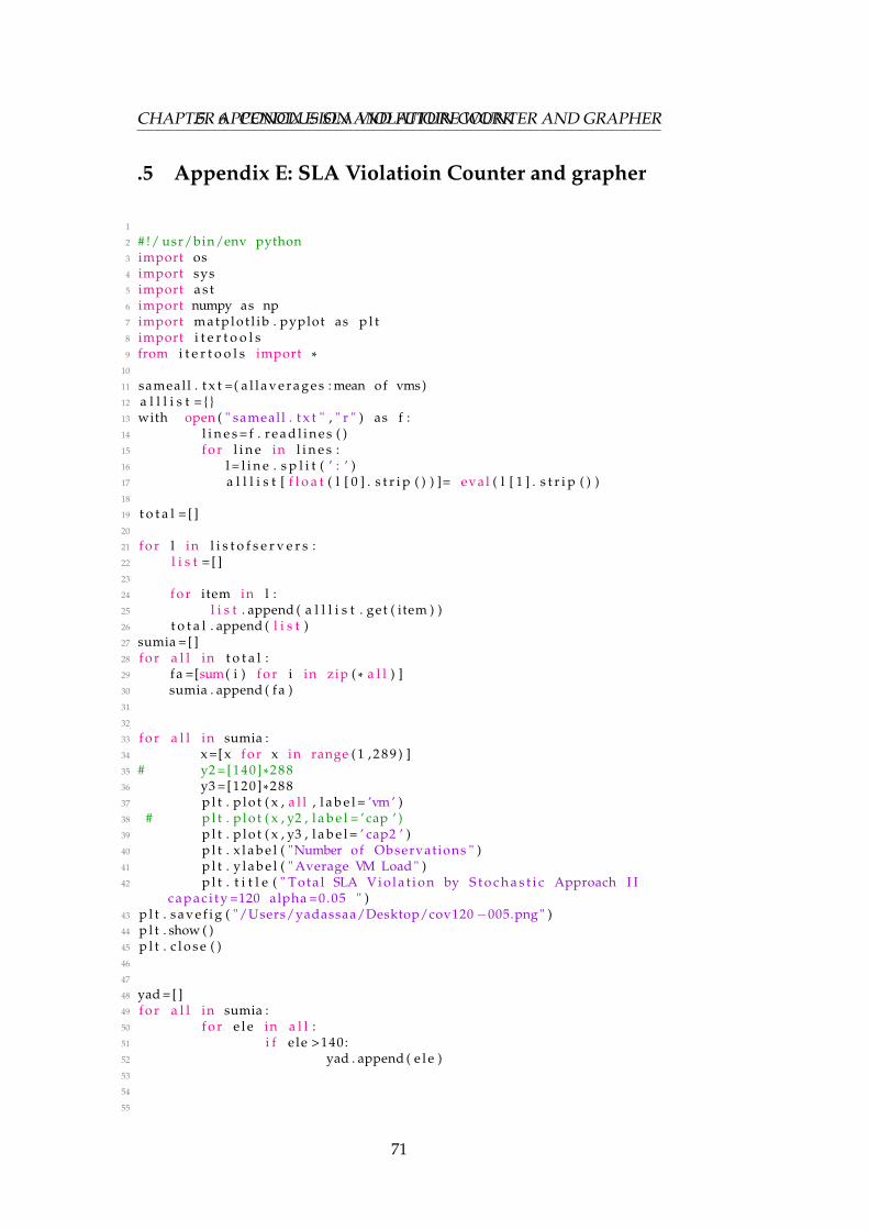
CHAPTER 6. CONCLUSION AND FUTURE WORK.5. APPENDIX E: SLA VIOLATIOIN COUNTER AND GRAPHER
.5 Appendix E: SLA Violatioin Counter and grapher
1
2 # !/ usr/bin/env python3 import os4 import sys5 import a s t6 import numpy as np7 import m a t p l o t l i b . pyplot as p l t8 import i t e r t o o l s9 from i t e r t o o l s import *
10
11 sameall . t x t =( a l l a v e r a g e s : mean of vms)12 a l l l i s t = { }13 with open ( " sameall . t x t " , " r " ) as f :14 l i n e s = f . r e a d l i n e s ( )15 f o r l i n e in l i n e s :16 l = l i n e . s p l i t ( ’ : ’ )17 a l l l i s t [ f l o a t ( l [ 0 ] . s t r i p ( ) ) ]= eval ( l [ 1 ] . s t r i p ( ) )18
19 t o t a l = [ ]20
21 f o r l in l i s t o f s e r v e r s :22 l i s t = [ ]23
24 f o r item in l :25 l i s t . append ( a l l l i s t . get ( item ) )26 t o t a l . append ( l i s t )27 sumia = [ ]28 f o r a l l in t o t a l :29 fa =[sum( i ) f o r i in zip ( * a l l ) ]30 sumia . append ( fa )31
32
33 f o r a l l in sumia :34 x =[ x f o r x in range ( 1 , 2 8 9 ) ]35 # y2 =[140] *28836 y3 =[120] *28837 p l t . p l o t ( x , a l l , l a b e l = ’vm ’ )38 # p l t . p l o t ( x , y2 , l a b e l = ’ cap ’ )39 p l t . p l o t ( x , y3 , l a b e l = ’ cap2 ’ )40 p l t . x l a b e l ( "Number of Observations " )41 p l t . y l a b e l ( " Average VM Load " )42 p l t . t i t l e ( " Tota l SLA V i o l a t i o n by S t o c h a s t i c Approach I I
c a p a c i t y =120 alpha =0.05 " )43 p l t . s a v e f i g ( "/Users/yadassaa/Desktop/cov120−005.png " )44 p l t . show ( )45 p l t . c l o s e ( )46
47
48 yad = [ ]49 f o r a l l in sumia :50 f o r e l e in a l l :51 i f e le >140:52 yad . append ( e l e )53
54
55
71

.5. APPENDIX E: SLA VIOLATIOIN COUNTER AND GRAPHERCHAPTER 6. CONCLUSION AND FUTURE WORK
56
Listing 5: SLA Violation counter and grapher
72
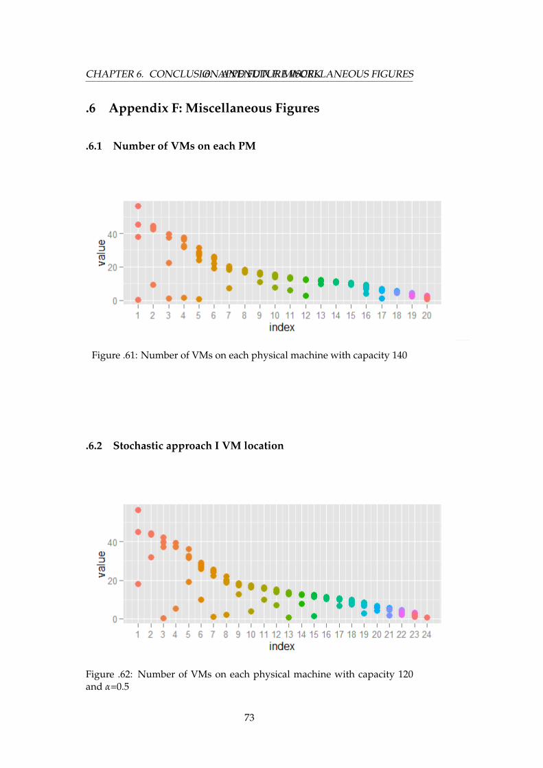
CHAPTER 6. CONCLUSION AND FUTURE WORK.6. APPENDIX F: MISCELLANEOUS FIGURES
.6 Appendix F: Miscellaneous Figures
.6.1 Number of VMs on each PM
Figure .61: Number of VMs on each physical machine with capacity 140
.6.2 Stochastic approach I VM location
Figure .62: Number of VMs on each physical machine with capacity 120and α=0.5
73
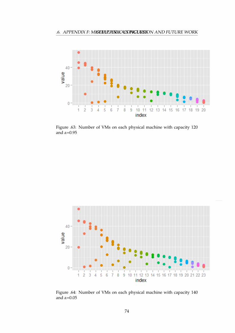
.6. APPENDIX F: MISCELLANEOUS FIGURESCHAPTER 6. CONCLUSION AND FUTURE WORK
Figure .63: Number of VMs on each physical machine with capacity 120and α=0.95
Figure .64: Number of VMs on each physical machine with capacity 140and α=0.05
74
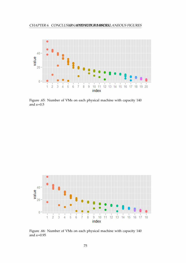
CHAPTER 6. CONCLUSION AND FUTURE WORK.6. APPENDIX F: MISCELLANEOUS FIGURES
Figure .65: Number of VMs on each physical machine with capacity 140and α=0.5
Figure .66: Number of VMs on each physical machine with capacity 140and α=0.95
75
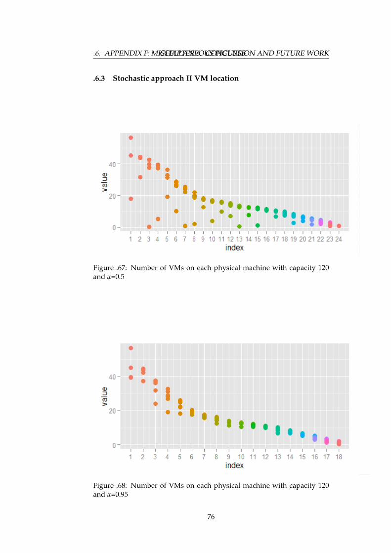
.6. APPENDIX F: MISCELLANEOUS FIGURESCHAPTER 6. CONCLUSION AND FUTURE WORK
.6.3 Stochastic approach II VM location
Figure .67: Number of VMs on each physical machine with capacity 120and α=0.5
Figure .68: Number of VMs on each physical machine with capacity 120and α=0.95
76
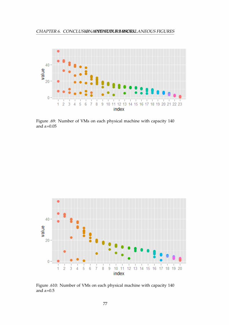
CHAPTER 6. CONCLUSION AND FUTURE WORK.6. APPENDIX F: MISCELLANEOUS FIGURES
Figure .69: Number of VMs on each physical machine with capacity 140and α=0.05
Figure .610: Number of VMs on each physical machine with capacity 140and α=0.5
77
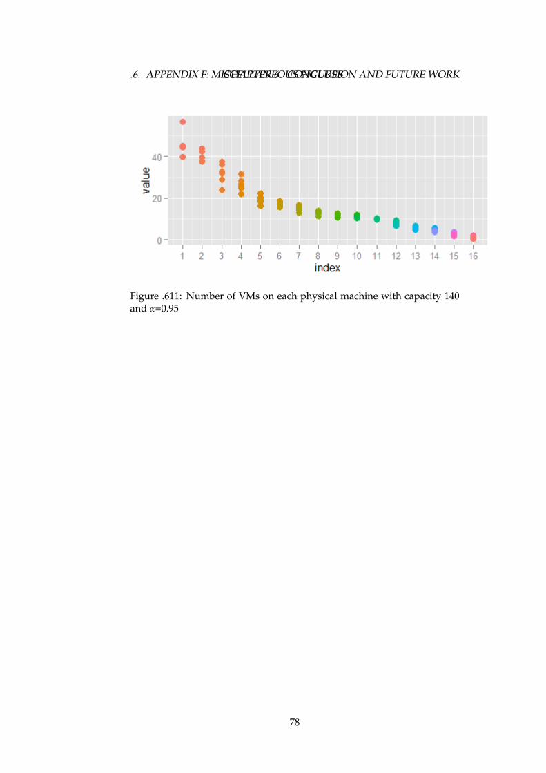
.6. APPENDIX F: MISCELLANEOUS FIGURESCHAPTER 6. CONCLUSION AND FUTURE WORK
Figure .611: Number of VMs on each physical machine with capacity 140and α=0.95
78
Bibliography
[1] Amany Abdelsamea et al. ‘Virtual Machine Consolidation Chal-lenges: A Review’. In: International Journal of Innovation and AppliedStudies (2014), pp. 1504–1516.
[2] Hadi Goudarzi et al. ‘SLA-based Optimization of Power and Migra-tion Cost in Cloud Computing’. In: 2012 12th IEEE/ACM InternationalSymposium on Cluster, Cloud and Grid Computing (2012), pp. 172–179.
[3] Heena Kaushar et al. ‘omparison of SLA based Energy Efficient Dy-namic Virtual Machine Consolidation Algorithms’. In: InternationalJournal of Computer Applications 102 (16 2014), pp. 31–36.
[4] Jian Tan et al. ‘Exploiting Resource Usage Patterns for Better Utiliz-ation Prediction’. In: 2011 31st International Conference on DistributedComputing Systems Workshops 8 (4 2011).
[5] Kihwan Choi et al. ‘Dynamic Voltage and Frequency Scaling basedon Workload Decomposition’. In: ACM (2004), pp. 1–6.
[6] Kishaloy Halder et al. ‘Risk Aware Provisioning and ResourceAggregation based Consolidation of Virtual Machines’. In: 2012 IEEEFifth International Conference on Cloud Computing (2012), pp. 598–605.
[7] Norman Bobroff et al. ‘Dynamic Placement of Virtual Machines forManaging SLA Violations’. In: 2012 13th International Conference onParallel and Distributed Computing, Applications and Technologies (2007),pp. 119–128.
[8] P. Getzi Jeba et al. ‘LIVE VM MIGRATION TECHNIQUES INCLOUD ENVIRONMENT – A SURVEY’. In: Proceedings of 2013IEEE Conference on Information and Communication Technologies (2013),pp. 104–113.
[9] Rina Pangigrahy et al. ‘Heuristics for Vector Bin Packing’. In:Microsoft Research (Unpublished 2011).
[10] Wen Chengjian et al. ‘Dynamic Power Saving via Least-Square Self-Tuning Regulator in the Virtualized Computing Systems’. In: TheEditorial Office of JSSC Springer (2012).
[11] Anton Beloglazov, Jemal Abawajy and Rajkumar Buyya. ‘Energy-aware resource allocation heuristics for efficient management of datacenters for Cloud computing’. In: Future Generation Computer Systems28.5 (2012), pp. 755–768.
79

BIBLIOGRAPHY BIBLIOGRAPHY
[12] Anton Beloglazov and Rajkumar Buyya. ‘OpenStack Neat: a frame-work for dynamic and energy-efficient consolidation of virtual ma-chines in OpenStack clouds’. In: Concurrency and Computation:Practiceand Experience (2014).
[13] Anton Beloglazov and Rajkumar Buyya. ‘Optimal Online Determin-istic Algorithms and Adaptive Heuristics for Energy and Perform-ance Efficient Dynamic Consolidation of Virtual Machines in CloudData Centers’. In: 24.13 (Sept. 2012), pp. 1397–1420.
[14] Zhibo Cao and Shoubin Dong. ‘Dynamic VM Consolidation forEnergy-Aware and SLA Violation Reduction in Cloud Computing’.In: Parallel and Distributed Computing, Applications and Technologies(PDCAT), 2012 13th International Conference on. Dec. 2012, pp. 363–369. DOI: 10.1109/PDCAT.2012.68.
[15] Cloudsim. What is CloudSim. Feb. 2015. URL: https://code.google.com/p/cloudsim/wiki/FAQ#1.%20_What_is_CloudSim_?_What_does_it_do_and_what_doesn’t_it_d.
[16] Pierre Delforge. ‘America’s Data Centers Consuming and WastingGrowing Amounts of Energy’. In: http://www.nrdc.org/energy/data-center-efficiency-assessment.asp (2014).
[17] Eamonn. What is the difference between IaaS,SaaS,PaaS? Feb. 2015. URL:https://www.computenext.com/blog/when-to-use-saas-paas-and-iaas/.
[18] Peter mell etal. The NIST Definition of Cloud Computing. 2011. URL:http://csrc.nist.gov/publications/nistpubs/800-145/SP800-145.pdf.
[19] Xiaobo Fan, Wolf-Dietrich Weber and Luiz Andre Barroso. ‘PowerProvisioning for a Warehouse-sized Computer’. In: Proceedings of the34th Annual International Symposium on Computer Architecture. ISCA’07. ACM, 2007, pp. 13–23.
[20] Bill Kleyman. Data Center Optimization. Jan. 2014. URL: http://www.datacenterknowledge . com / archives / 2014 / 01 / 22 / five - great - ways -optimize-data-center/.
[21] Bill Kleyman. Understanding the Virtualization market. 2015. URL: http://www.datacenterknowledge.com/archives/2012/08/01/hypervisor-101-a-look-hypervisor-market/.
[22] Jonathan G Koomey. ‘Worldwide electricity used in data centers’. In:Lawrence Berkeley National Laboratory, USA (2008), pp. 1–9.
[23] Century Link. Cloud Data Center Service Level Agreement. 2015. URL:http://www.centurylinktechnology.com/en- gb/legal/sla/cloud- data-center.
[24] Tania Lorido-Botrán, José Miguel-Alonso and Jose Antonio Lozano.Auto-scaling Techniques for Elastic Applications in Cloud Environments.Research EHU-KAT-IK. Department of Computer Architecture andTechnology, UPV/EHU, 2012.
80

BIBLIOGRAPHY BIBLIOGRAPHY
[25] Zar Lwin and Thandar Thein. ‘Correlation based VMs PlacementResource Provision’. In: International Journal of Computer ScienceInformation Technology (IJCSIT) Vol 5, No 1, February 2013 (2013),pp. 95–107.
[26] Xiaoqiao Meng et al. ‘Efficient Resource Provisioning in ComputeClouds via VM Multiplexing’. In: Proceedings of the 7th InternationalConference on Autonomic Computing. ICAC ’10. New York, NY, USA:ACM, 2010, pp. 11–20.
[27] Micrsoft. About Virtual Machine Placement. Feb. 2015. URL: https : //technet.microsoft.com/en-us/library/bb740817.aspx.
[28] Margaret Rouse. Virtualization. Feb. 2015. URL: http://searchservervirtualization.techtarget.com/definition/virtualization.
[29] M. Sedaghat et al. ‘Divide the Task, Multiply the Outcome: Cooper-ative VM Consolidation’. In: Cloud Computing Technology and Sci-ence (CloudCom), 2014 IEEE 6th International Conference on. Dec. 2014,pp. 300–305. DOI: 10.1109/CloudCom.2014.81.
[30] Virtualization. Feb. 2015. URL: http : / / en . wikipedia . org / wiki /Virtualization.
[31] Wikipedia. Bin Packing Problem. March 2015. URL: http://en.wikipedia.org/wiki/Bin_packing_problem.
[32] Wikipedia. Virtual Machine. 2015. URL: http://en.wikipedia.org/wiki/Virtual_machine.
[33] A. Wolke and C. Pfeiffer. ‘Improving Enterprise VM Consolidationwith High-Dimensional Load Profiles’. In: Cloud Engineering (IC2E),2014 IEEE International Conference on. Mar. 2014, pp. 283–288.
[34] Xiaodong Zhang et al. ‘SmartRelationship: A VM Relationship De-tection Framework for Cloud Management’. In: Proceedings of the 6thAsia-Pacific Symposium on Internetware on Internetware. INTERNET-WARE 2014. ACM, 2014, pp. 72–75.
81
![Consolidation of reward memory during sleep does not ...consolidation processes select the most relevant for long-term storage [1, 2]. During ... than directly participating in sleep-dependent](https://img.pdfslide.net/doc/110x75/60c0a1945257057b50130ec5/consolidation-of-reward-memory-during-sleep-does-not-consolidation-processes.jpg)


![qbr1-1info.brightgauge.com/hubfs/qbr1-1.pdf[QBR] SLA Statistics by I-HT Normal Priority - Last 90 Days PRIORITY TOTAL MET SLA - 65 Normal MET SLA MET RESPONSE SLA RESPONSE SLA MET](https://img.pdfslide.net/doc/110x75/613b13f2f8f21c0c8268ccdd/qbr1-1info-qbr-sla-statistics-by-i-ht-normal-priority-last-90-days-priority.jpg)


![[PPT]Teamwork · Web viewPsycholinguistic aspects of interlanguage Second language acquisition SLA * * * * * * * * * * L1 Transfer * SLA * L1 transfer * SLA * Types of transfer * SLA](https://img.pdfslide.net/doc/110x75/5a9fa7b87f8b9a6c178d045e/pptteamwork-viewpsycholinguistic-aspects-of-interlanguage-second-language-acquisition.jpg)