Time domain earthquake response analysis method for 2-D ...ssu.ac.ir/cms/fileadmin/user_upload/Moavenatha/Mposhtibani/Mdaftar... · Time domain earthquake response analysis method

Structural Engineering and Mechanics, Vol. 15, No. 6 (2003) 717-733 717

Time domain earthquake response analysis method for 2-D soil-structure interaction systems

Doo Kie Kim†

Department of Civil Engineering, Kunsan National University, San 68, Miryong-Dong, Kunsan, Jeonbuk 573-701, Korea

Chung-Bang Yun‡

Department of Civil Engineering, Korea Advanced Institute of Science and Technology,373-1, Kusong-Dong, Yusong-Ku, Daejeon 305-701, Korea

(Received July 29, 2002, Accepted March 19, 2003)

Abstract. A time domain method is presented for soil-structure interaction analysis under seismicexcitations. It is based on the finite element formulation incorporating infinite elements for the far fieldsoil region. Equivalent earthquake input forces are calculated based on the free field responses along theinterface between the near and far field soil regions utilizing the fixed exterior boundary method in thefrequency domain. Then, the input forces are transformed into the time domain by using inverse Fouriertransform. The dynamic stiffness matrices of the far field soil region formulated using the analyticalfrequency-dependent infinite elements in the frequency domain can be easily transformed into thecorresponding matrices in the time domain. Hence, the response can be analytically computed in the timedomain. A recursive procedure is proposed to compute the interaction forces along the interface and theresponses of the soil-structure system in the time domain. Earthquake response analyses have been carriedout on a multi-layered half-space and a tunnel embedded in a layered half-space with the assumption ofthe linearity of the near and far field soil region, and results are compared with those obtained by theconventional method in the frequency domain.

Key words: soil-structure interaction; analytical frequency-dependent infinite element; earthquakeresponse analysis; time domain analysis; recursive procedure.

1. Introduction

The earthquake responses of massive civil engineering structures may be influenced by the soil-structure interaction as well as the dynamic characteristics of the excitations and the structures. Theeffect of the soil-structure interaction is noticeable especially for stiff and massive structures restingon the relatively soft ground. It may cause the dynamic characteristics of the structural responsealtered significantly. Thus the interaction effects have to be considered in the dynamic analysis ofthe structures in a semi-infinite soil medium (Wolf 1985, Betti et al. 1993).

† Assistant Professor‡ Professor

718 Doo Kie Kim and Chung-Bang Yun

Two important things that may distinguish the soil-structure interaction system from the generalstructural dynamic system are the unbounded nature and the nonlinear characteristics of the soilmedium. In general, the radiational damping in an unbounded soil medium can be described moreeasily in the frequency domain than in the time domain, since it is dependent on the excitationfrequencies (Wolf 1985). On the other hand, the nonlinear behavior of the soil medium can beconsidered more easily in the time domain (Wolf 1988, Wolf and Song 1996). Thus supplementarytreatments of soil-structure interaction in the frequency and time domains may be needed toconsider both characteristics of the soil medium. At present, most of the well-known computerprograms for soil-structure interaction analysis are based on the frequency domain analysisincorporating the equivalent linearization technique to consider the nonlinearity of the soil medium(Seed and Idriss 1970, Kramer 1996, Lysmer et al. 1975, ASD International 1985, Lysmer et al.1988, Tzong and Penzien 1983).

In recent years, several time domain methods have been proposed to study nonlinear behaviors ofthe soil medium, effects of pore water, and nonlinear conditions along the interface between soil andstructure. One method is the coupling of the boundary and the finite element methods (Karabalisadn Beskos 1985, Estorff 1991, Guan and Novak 1994). In this method the structure and the nearfield soil region are modeled using finite elements, while the far field soil region is representedusing boundary elements. However, it has been generally difficult to derive fundamental solutions inlayered soils and to couple the boundary elements with the finite elements. In recent researches,significant advance in the time domain has been made in this area (Song and Wolf 1999, Zhanget al. 1999). This method, which does not require fundamental solution, has been successfully usedin coupling with finite elements and applied for three dimensional soil-structure interactions in the timedomain. Another method is the one using the transformation of the dynamic stiffness matrix into theterms in the time domain (Hayashi and Katukura 1990). However, the dynamic stiffness matrix forthe far field region is usually obtained numerically at each frequency. Therefore, the transformationhas to be carried out numerically using discrete Fourier transform or discrete z-transform, whichrequires tremendous computational time and huge computer-memory for realistic problems.

This paper presents a time domain method for soil-structure interaction analysis under seismicloadings. It is based on the finite element formulation incorporating analytical frequency-dependentinfinite elements for the far field soil region (Yun et al. 2000, Kim and Yun 2000). The equivalentearthquake input forces are calculated based on the free field responses (Wolf and Obernhuber 1982)along the interface between the near and far field soil regions using the fixed exterior boundary method(Zhao and Valliappan 1993). The earthquake input forces are computed in the frequency domain, thenconverted into the time domain. The interaction forces along the interface during the earthquakeresponse analysis are computed using a recursive procedure developed in this study. For verification,earthquake response analysis has been carried out for a multi-layered half-space with the assumption ofthe linearity of the near- and far field soil region, and the results are compared with the free fieldresponses obtained by the conventional frequency domain method (Wolf and Obernhuber 1982, Zhaoand Valliappan 1993, Zhang and Zhao 1988). Earthquake response analysis has been also performed fora tunnel embedded in a layered half-space to show the applicability of the proposed method in the field.

2. Modeling of far field soil region

The structure and the near field soil region are modeled using 9-node plane strain finite elements,

Time domain earthquake response analysis method for 2-D soil-structure interaction systems719

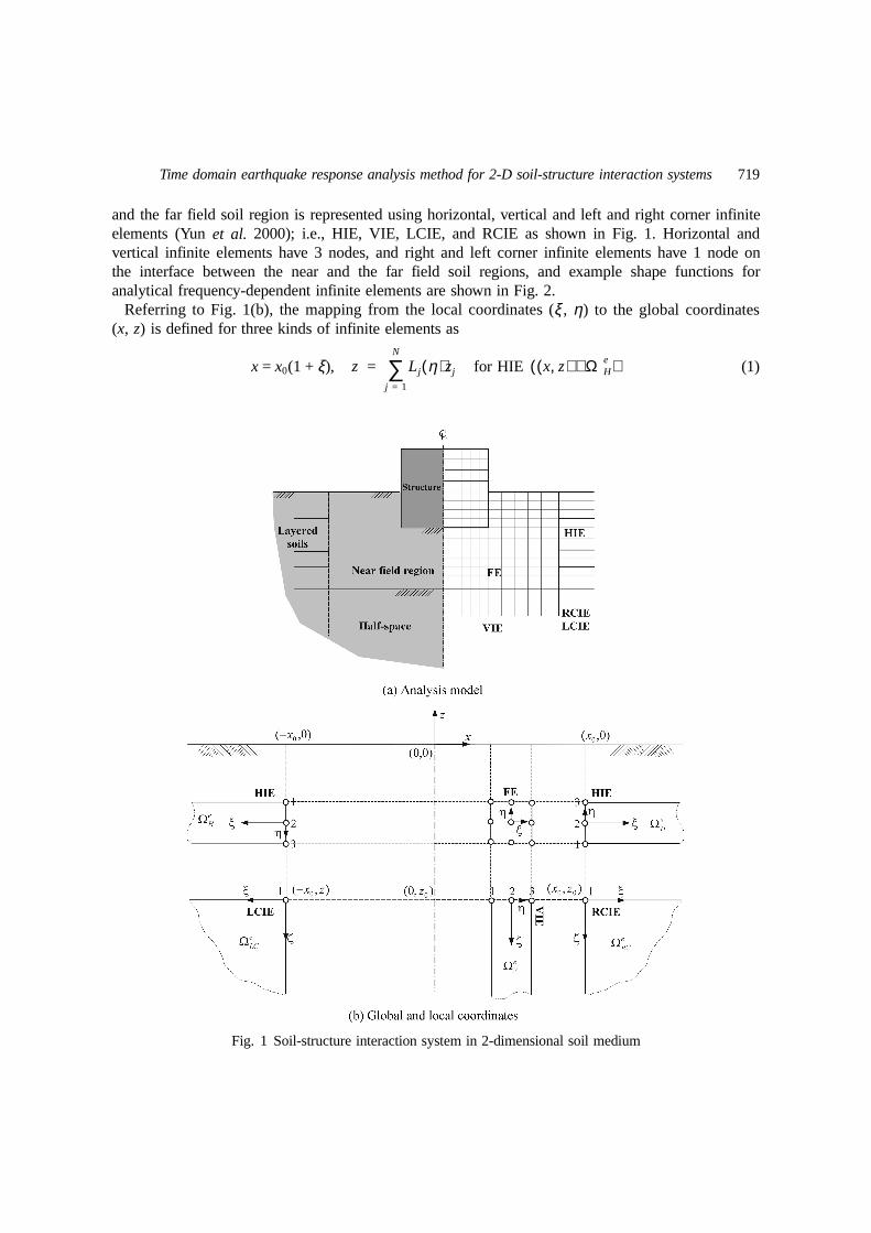
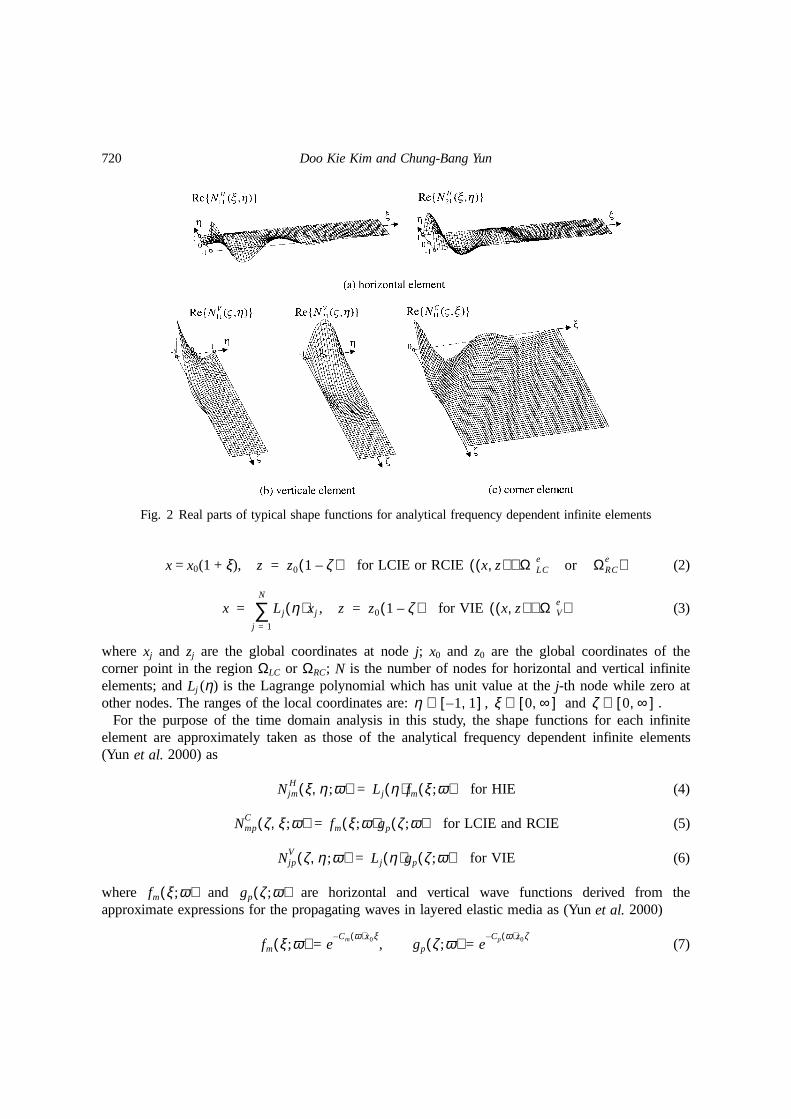
and the far field soil region is represented using horizontal, vertical and left and right corner infiniteelements (Yun et al. 2000); i.e., HIE, VIE, LCIE, and RCIE as shown in Fig. 1. Horizontal andvertical infinite elements have 3 nodes, and right and left corner infinite elements have 1 node onthe interface between the near and the far field soil regions, and example shape functions foranalytical frequency-dependent infinite elements are shown in Fig. 2.

Referring to Fig. 1(b), the mapping from the local coordinates (ξ, η) to the global coordinates(x, z) is defined for three kinds of infinite elements as

x = x0(1 + ξ), for HIE (1)z Lj η( )zj

j 1=

N

∑= x z,( ) ΩHe∈( )

Fig. 1 Soil-structure interaction system in 2-dimensional soil medium


x = x0(1 + ξ), for LCIE or RCIE (2)

, for VIE (3)

where xj and zj are the global coordinates at node j; x0 and z0 are the global coordinates of thecorner point in the region ΩLC or ΩRC; N is the number of nodes for horizontal and vertical infiniteelements; and Lj (η) is the Lagrange polynomial which has unit value at the j-th node while zero atother nodes. The ranges of the local coordinates are: , and .

For the purpose of the time domain analysis in this study, the shape functions for each infiniteelement are approximately taken as those of the analytical frequency dependent infinite elements(Yun et al. 2000) as

for HIE (4)

for LCIE and RCIE (5)

for VIE (6)

where and are horizontal and vertical wave functions derived from theapproximate expressions for the propagating waves in layered elastic media as (Yun et al. 2000)

(7)

z z0 1 ζ–( )= x z,( ) ΩLCe or ΩRC

e∈( )

x Lj η( )xj

j 1=

N

∑= z z0 1 ζ–( )= x z,( ) ΩVe∈( )

η 1– 1,[ ]∈ ξ 0 ∞ ],[∈ ζ 0 ∞ ],[∈

NjmH ξ η;ω,( ) Lj η( )fm ξ;ω( )=

NmpC ζ ξ;ω,( ) fm ξ;ω( )gp ζ;ω( )=

NjpV ζ η;ω,( ) Lj η( )gp ζ;ω( )=

fm ξ;ω( ) gp ζ;ω( )

fm ξ;ω( ) eCm ω( )x0ξ–

= , gp ζ;ω( ) eCp ω( )z0ζ–

=

Fig. 2 Real parts of typical shape functions for analytical frequency dependent infinite elements


where

, (8)

where cs, cp, and are wave velocities for S-wave, P-wave and the mean value of the l-thRayleigh wave (l = 1, ..., Nr) in the frequency range of concern; and Nr is the number of Rayleighwaves employed in the displacement approximation. The positive constant, a, in Eq. (8) is related tothe geometric attenuation, and taken to be the same for all wave components. Validity of theapproximation in Eqs. (7) and (8) was extensively discussed in Yun et al. (2000).

The mass and stiffness component matrices of the infinite element associated with the j-th and thek-th shape functions are defined as

(9)

(10)

where ρ is the mass density; I and D are the (2 × 2) identity and the elasticity matrices; and Bj andBk are the strain-displacement matrices associated with shape function Nj and Nk, respectively.

Employing the shape functions with the wave functions described in Eqs. (7) and (8), the massand stiffness matrices for each infinite element can be obtained in analytical forms of the excitingfrequency and constant matrices as (Yun et al. 2000)

(11)

(12)

where and are real-valued constant matrices if the material damping inthe far field soil is ignored, which is generally much smaller than the radiation damping.

Assembling the mass and stiffness matrices of the analytical frequency-dependent infiniteelements, the dynamic stiffness matrix of the far field soil region, , can be obtained as (Yunet al. 2000)

(13)

where , and are real-valued constant matrices if the material damping in the far fieldsoil is ignored :

(14a)

Cm ω( ) a iω+( )

1cs

----

1cp

----

1crl

------

= Cp ω( ) a iω+( )

1cs

----

1cp

----

=

crl

mjk ρ NjTNkdΩI

Ω

∫=

kjk BjTDBkdΩ

Ω∫=

M e( ) ω( ) 1a iω+----------------M0

e( ) 1

a iω+( )2-----------------------M1

e( )+=

K e( ) ω( ) K0e( ) a iω+( )K1

e( ) 1a iω+----------------K2

e( )+ +=

M0e( ) M1

e( ) K0e( ) K1

e( ), , , K2e( )

SeeF ω( )

SeeF ω( ) S0

F iωS1F 1

a iω+----------------S2

F 1

a iω+( )2-----------------------S3

F+ + +=

S0F S1

F S2F, , S3

F

S0F K0

F aK1F aM0

F– M1F+ +=


(14b)

(14c)

(14d)

in which and are the assemblages of the element-level matrices and respectively.

3. Earthquake response analysis in time domain

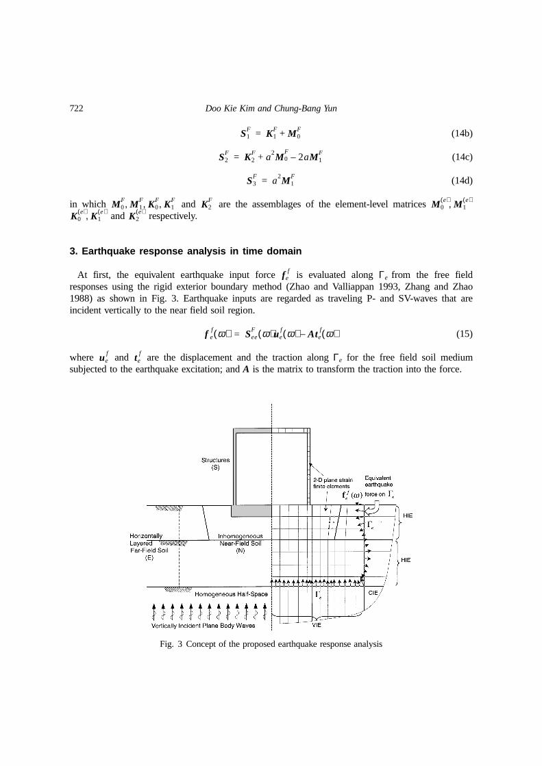
At first, the equivalent earthquake input force is evaluated along Γe from the free fieldresponses using the rigid exterior boundary method (Zhao and Valliappan 1993, Zhang and Zhao1988) as shown in Fig. 3. Earthquake inputs are regarded as traveling P- and SV-waves that areincident vertically to the near field soil region.

(15)

where and are the displacement and the traction along Γe for the free field soil mediumsubjected to the earthquake excitation; and A is the matrix to transform the traction into the force.

S1F K1

F M0F+=

S2F K2

F a2M0

F2aM1

F–+=

S3F a

2M1

F=

M0F M1

F K0F K1

F, , , K2F M0

e( ) M1e( ),

K0e( ) K1

e( ), K2e( )

fef

f ef ω( ) See

F ω( )uef ω( ) Ate

f ω( )–=

uef te

f

Fig. 3 Concept of the proposed earthquake response analysis


Then, the equation of motion for the soil-structure interaction system subjected to can bewritten in the frequency domain as (Wolf 1985)

(16)

where subscript n stands for the degrees-of-freedom (DOF’s) of the structure and the near field soilregion, while e denotes those on the interface Γe. For the computational convenience, Eq. (16) canbe rewritten as

(17)

(18)

where may be defined as the interaction force which depends on the response of the interfaceΓe with the far field soil region.

For time domain analysis, the interaction force can be transformed as (Wolf 1988, Wolfand Song 1996)

(19)

where is the inverse Fourier transform of , which can be obtained from Eq. (13) in ananalytical form as (Kim and Yun 2000)

(20)

(21)

where H(t) is unit step function; and δ (t) and are Dirac-delta function and its derivativerespectively. From Eqs. (19) and (21), the interaction force can be also obtained analytically as(Kim and Yun 2000)

(22)

Finally, the time domain equation of motion for the soil-structure interaction system can bederived from Eqs. (17) and (22) as

(23)

where Mnn, Mne, Men, Mee, Knn, Kne, Ken, and Kee are the conventional mass and stiffness matrices for

f ef ω( )

Snn ω( ) Sne ω( )

Sen ω( ) See ω( ) SeeF ω( )+

un ω( )

ue ω( ) 0

f ef ω( )

=

Snn ω( ) Sne ω( )Sen ω( ) See ω( )

un ω( )

ue ω( ) 0

f ef ω( ) fe ω( )+

=

fe ω( ) SeeF ω( )– ue ω( )=

fe ω( )

fe ω( )

fe t( ) SeeF t τ–( )ue τ( )dτ

0

t∫–=

SeeF t( ) See

F ω( )

SeeF t( ) F

1– SeeF ω( ) 1

2π------ See

F ω( )ei ωtdω−∞+ ∞∫==

SeeF t( ) S0

Fδ t( ) S1Fδ· t( ) S2

Fe at– H t( ) S3Fte at– H t( )+ + +=

δ· t( )

fe t( ) S0Fue t( )– S1

Fu·e t( )– S2F t τ–( )S3

F+ e a t τ–( )– ue τ( )dτ0

t∫–=

Mnn Mne

Men Mee

u··n t( )

u··e t( ) 0 0

0 S1F

u·n t( )

u·e t( ) Knn Kne

Ken Kee S0F

+

un t( )

ue t( )

+ +0

fef t( ) f e t( )+

=


the structure and the near field soil; is the equivalent earthquake input force along Γe obtainedfrom inverse Fourier Transform of ; and is the third term of the interaction force fe(t) inEq. (22) as

(24)

In Eq. (23), a nonlinear restoring force and linear damping in the near field as well as and can be included for more practical and robust application of the proposed method. However,

only the linear radiational damping of the soil region in the present paper is considered.

4. Recursive procedure for response in time domain

The present recursive procedure in the time domain is basically using the Newmark-Beta methodalthough approximations at various stages are being made.

The new interaction force in Eq. (24) can be decomposed as

(25)

where

(26a)

(26b)

and (26c)

Numerical evaluation of the convolution integrals in Eqs. (26a)-(26c) would be very timeconsuming. Therefore an efficient recursive procedure is developed, assuming a linear variation ofthe responses between two adjacent times. The Eqs. (26a)-(26c) can be approximately rewritten intodiscrete time forms at t = n∆t as

(27a)

(27b)

fef t( )

fef ω( ) f e t( )

f e t( ) S2F t τ–( )S3

F+ e a t τ–( )– ue τ( )dτ

0

t∫–=

fef ω( )

f e t( )

f e t( )

f e t( ) f e1 t( ) f e2 t( ) f e t( )∆+ +=

f e1 t( ) S2Fe a t τ–( )– ue τ( )dτ

0

t t∆–∫–=

f e2 t( ) t τ–( )S3Fe a t τ–( )– ue τ( )dτ

0

t t∆–∫–=

f e t( )∆ S2F t τ–( )S3

F+ e a t τ–( )– ue τ( )dτt t∆–

t∫–=

f e1 t( ) e a t∆– f e1 t t∆–( ) S2Fe

2a t∆–

a2

t∆------------ 1 ea t∆ 1 a t∆–( )– [ ue t t∆–( )–=

1 a t∆ ea t∆–+ ue t 2 t∆–( ) ]–

f e2 t( ) 2e a t∆– f e2 t t∆–( ) e 2a t∆– f e2 t 2 t∆–( )–=

+S3F 1

a3 t∆---------- e 2a t∆– 2– 2a t∆– ea t∆ 2 a2 t∆( )2–( )+ ue t t∆–( )[

+e3a t∆– 2 a t∆ ea t∆ 4a t∆ 2a

2t∆( )2+( )+ + 22a t∆ 2 a t∆+( ) ue t 2 t∆–( )–

+e3a t∆– 2– 2a t∆– a

2t2∆( )– 2ea t∆+ ue t 3 t∆–( ) ]


(27c)

Incorporating the above equations, the Eq. (23) can be approximately rewritten into discrete timeforms at t = n∆t as

(28)

where α2, α3, β2 and β3 are real constants, which depend on a and ∆t, as

(29a)

(29b)

(29c)

(29d)

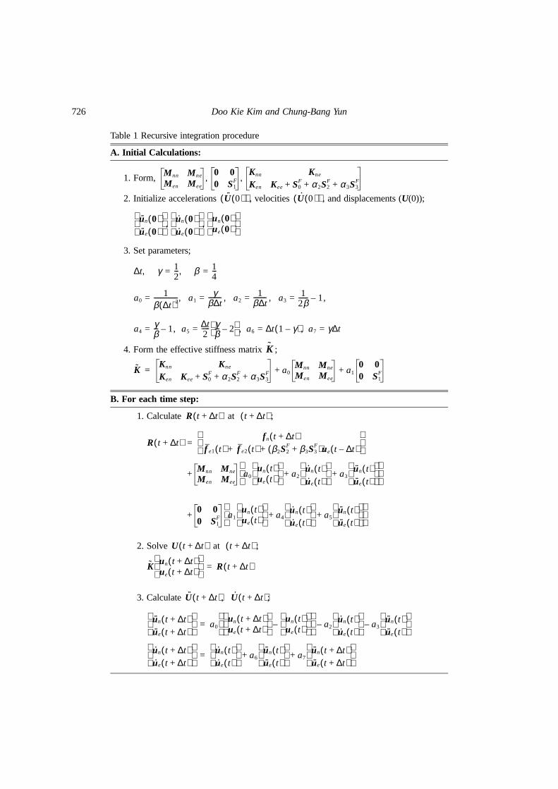
In the present study, it is noteworthy that the convolution integrals for and areevaluated recursively as finite sums of a few past terms of , , and . The recursiveprocedure for the numerical evaluation of the convolution integral in Eq. (28) is summarized inTable 1. In fact a similar procedure was proposed assuming a constant value of the response between two adjacent times by the present authors (Kim and Yun 2000). Hence the presentformulation based on the linear variation may be considered as an improved one. The present timedomain formulation based on the analytical frequency-dependent infinite elements is verystraightforward and computationally very efficient in comparison with the methods using numericaltransforms such as discrete Fourier transform or discrete z-transform, which usually require hugecomputational efforts (Wolf 1988, Wolf and Song 1996, Tzong and Penzien 1985).

5. Numerical examples

5.1 Free field responses of a layered soil medium

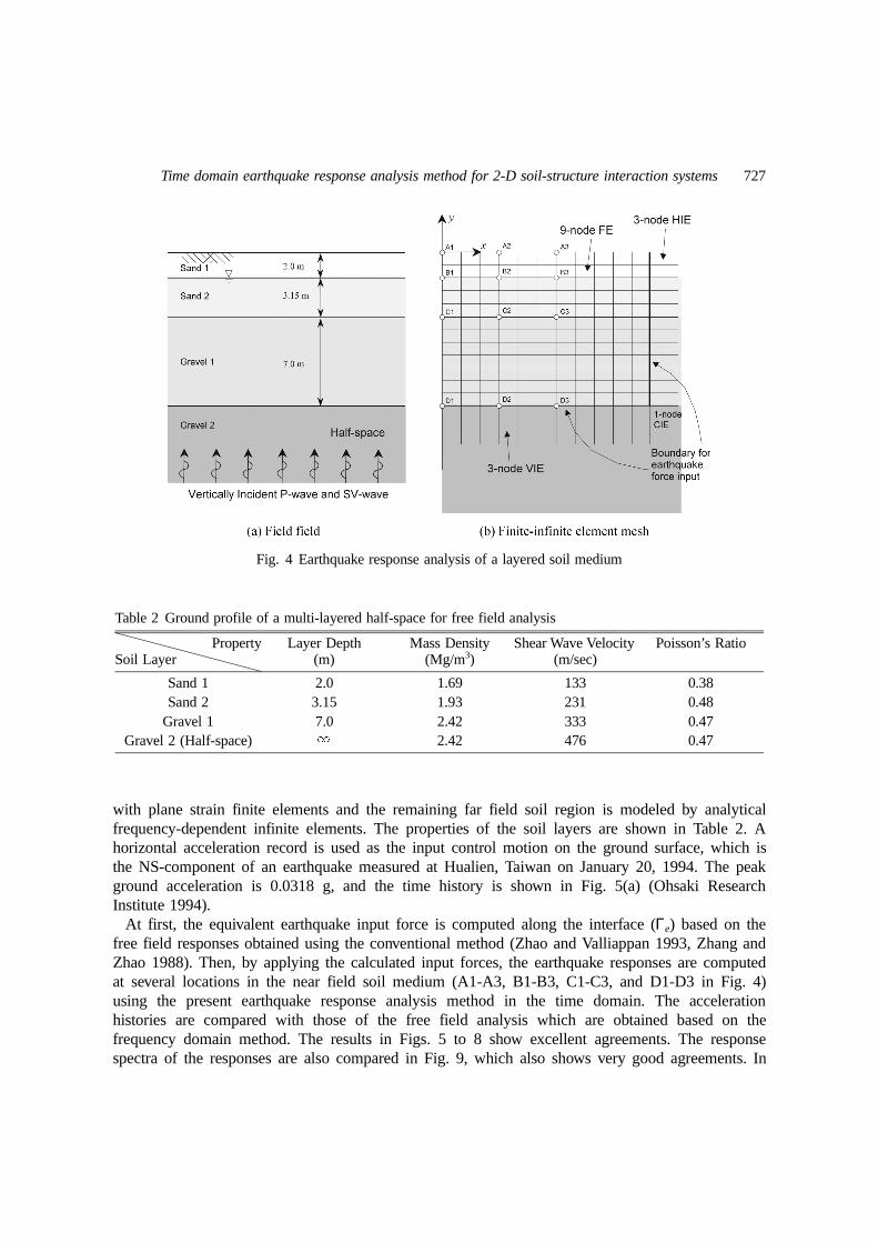
For verification of the proposed analysis procedure, earthquake response analysis of a multi-layered free field half-space shown in Fig. 4 is carried out. The near field soil region is discretized

f e t( )∆ S2F 1

a2 t∆---------- 1– a t∆ e a t∆–+ + [ ue t( ) 1 e a t∆– 1 a t∆+( )– ue t t∆–( ) ]+–=

S3F 1

a3 t∆---------- 2– a t∆ e a t∆– 2 a t∆+( )+ + [ ue t( )–

+ 2 e a t∆– 2 2a t∆ a2

t∆( )2+ +( )– ue t t∆–( ) ]

Mnn Mne

Mns Mee

u··n t( )

u··e t( ) 0 0

0 S1F

u·n t( )

u·e t( ) Knn Kne

Ken Kee S0F α2S2

F α3S3F+ + +

un t( )

ue t( )

+ +

0

f ef t( ) f e1 t( ) f e2 t( ) β2S2

F β3S3F+( )ue t t∆–( )+ + +

=

α21

a2

t∆---------- 1 a t∆ e a t∆–+ +– =

α31

a3

t∆---------- 2– a t∆ e a t∆– 2 a t∆+( )+ + =

β21

a2 t∆---------- 1– e a t∆– 1 a t∆+( )+ =

β31

a2 t∆---------- 2– e a t∆– 2 2a t∆ a2 t∆( )2+ +( )+ =

f e1 t( ) f e2 t( )f e1 t( ) f e2 t( ) ue t( )

ue t( )


Table 1 Recursive integration procedure

A. Initial Calculations:

1. Form,

2. Initialize accelerations , velocities , and displacements (U(0));

3. Set parameters;

4. Form the effective stiffness matrix ;

B. For each time step:

1. Calculate ;

2. Solve ;

3. Calculate

M nn Mne

Men Mee

0 00 S1

FKnn Kne

Ken Kee S0F α2S2

F α3S3F+ + +

, ,

U··

0( )( ) U·

0( )( )

u··n 0( )u··e 0( )

u·n 0( )

u·e 0( ) un 0( )

ue 0( )

, ,

t∆ γ 12---= β 1

4---=, ,

a01

β t∆( )2---------------= a1

γβ t∆--------= a2

1β t∆--------= a3

12β------ 1,–=, , ,

a4γβ--- 1,–= a5

t∆2----- γ

β--- 2– = , a6 t∆ 1 γ–( )= , a7 γ t∆=

K

KKnn Kne

Ken Kee S0F α2S2

F α3S3F+ + +

a0Mnn Mne

Men Meea1

0 00 S1

F++=

R t t∆+( ) at t t∆+( )

R t t∆+( )fn t t∆+( )

f e1 t( ) f e2 t( ) β2S2F β3S3

F+( )ue t t∆–( )+ +

=

+ Mnn Mne

Men Meea0

un t( )ue t( )

a2u·n t( )u·e t( )

a3u··n t( )u··e t( )

+ +

+0 00 S1

F a1un t( )ue t( )

a4u·n t( )u·e t( )

a5u··n t( )u··e t( )

+ +

U t t∆+( ) at t t∆+( )

Kun t t∆+( )ue t t∆+( )

R t t∆+( )=

U·· t t∆+( ) U· t t∆+( );,

u··n t t∆+( )u··e t t∆+( )

a0un t t∆+( )ue t t∆+( )

un t( )

ue t( )

– a2u·n t( )u·e t( )

a3u··n t( )u··e t( )

––

=

u·n t t∆+( )u·e t t∆+( )

u·n t( )

u·e t( )

a6u··n t( )u··e t( )

a7u··n t t∆+( )u··e t t∆+( )

+ +=


with plane strain finite elements and the remaining far field soil region is modeled by analyticalfrequency-dependent infinite elements. The properties of the soil layers are shown in Table 2. Ahorizontal acceleration record is used as the input control motion on the ground surface, which isthe NS-component of an earthquake measured at Hualien, Taiwan on January 20, 1994. The peakground acceleration is 0.0318 g, and the time history is shown in Fig. 5(a) (Ohsaki ResearchInstitute 1994).

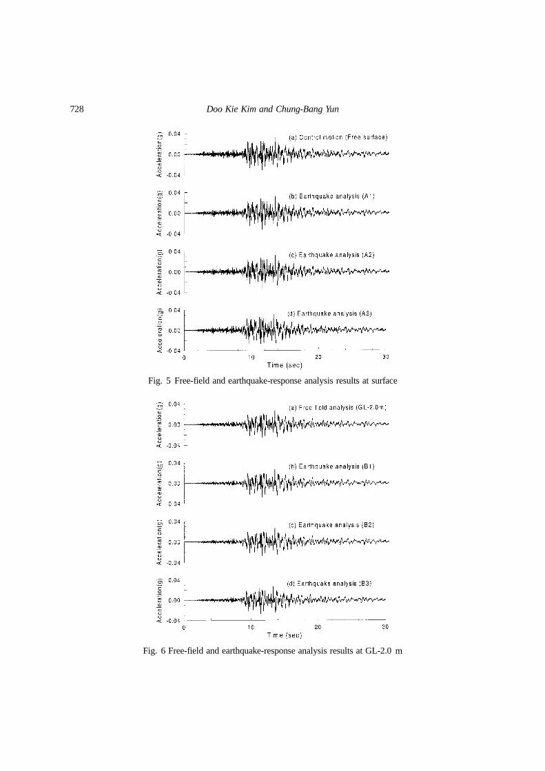
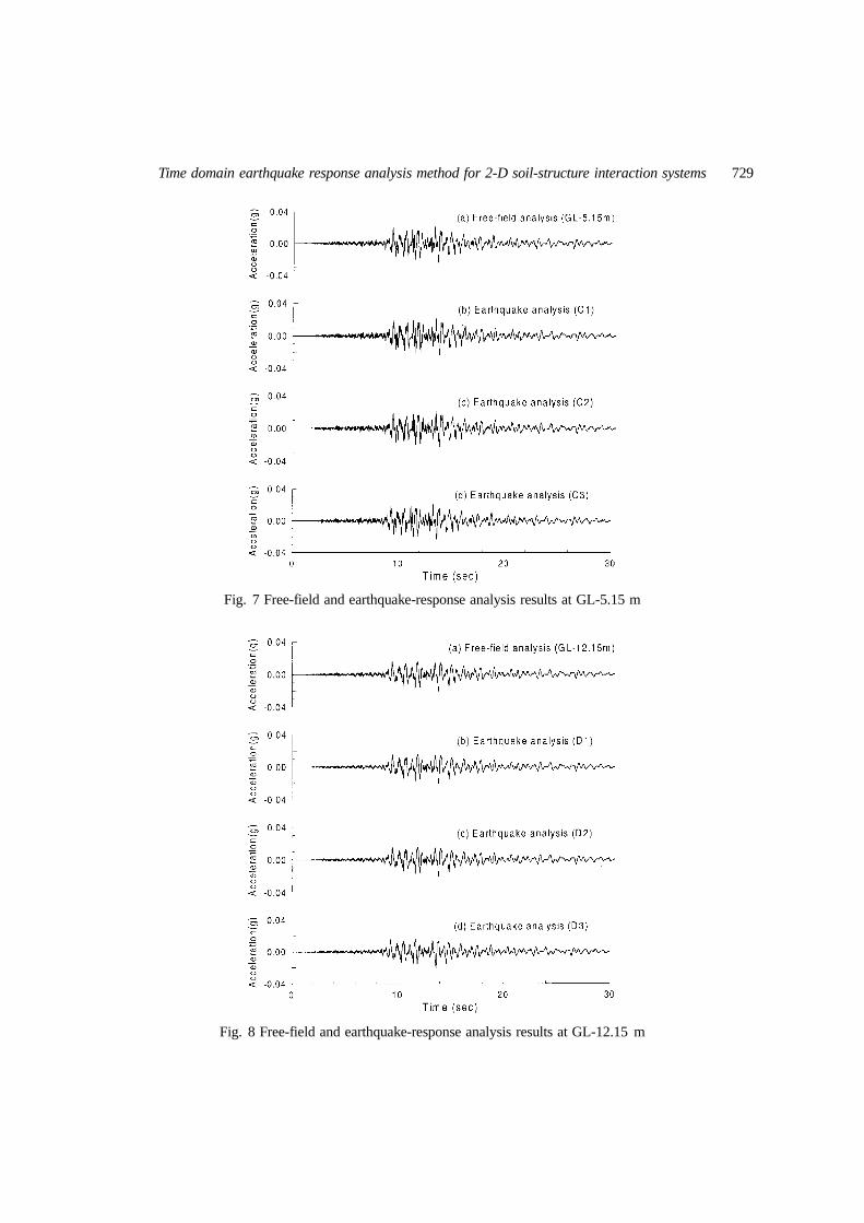
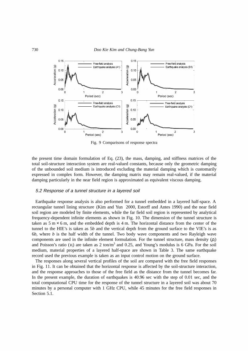
At first, the equivalent earthquake input force is computed along the interface (Γe) based on thefree field responses obtained using the conventional method (Zhao and Valliappan 1993, Zhang andZhao 1988). Then, by applying the calculated input forces, the earthquake responses are computedat several locations in the near field soil medium (A1-A3, B1-B3, C1-C3, and D1-D3 in Fig. 4)using the present earthquake response analysis method in the time domain. The accelerationhistories are compared with those of the free field analysis which are obtained based on thefrequency domain method. The results in Figs. 5 to 8 show excellent agreements. The responsespectra of the responses are also compared in Fig. 9, which also shows very good agreements. In

Fig. 4 Earthquake response analysis of a layered soil medium

Table 2 Ground profile of a multi-layered half-space for free field analysis

PropertySoil Layer

Layer Depth(m)

Mass Density(Mg/m3)

Shear Wave Velocity (m/sec)

Poisson’s Ratio

Sand 1 2.0 1.69 133 0.38Sand 2 3.15 1.93 231 0.48

Gravel 1 7.0 2.42 333 0.47Gravel 2 (Half-space) ó 2.42 476 0.47


Fig. 5 Free-field and earthquake-response analysis results at surface

Fig. 6 Free-field and earthquake-response analysis results at GL-2.0 m





the present time domain formulation of Eq. (23), the mass, damping, and stiffness matrices of thetotal soil-structure interaction system are real-valued constants, because only the geometric dampingof the unbounded soil medium is introduced excluding the material damping which is customarilyexpressed in complex form. However, the damping matrix may remain real-valued, if the materialdamping particularly in the near field region is approximated as equivalent viscous damping.

5.2 Response of a tunnel structure in a layered soil

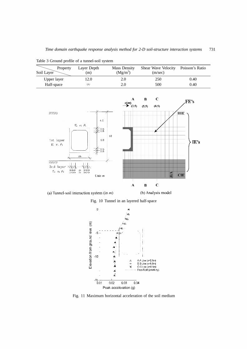
Earthquake response analysis is also performed for a tunnel embedded in a layered half-space. Arectangular tunnel lining structure(Kim and Yun 2000, Estorff and Antes 1990) and the near fieldsoil region are modeled by finite elements, while the far field soil region is represented by analyticalfrequency-dependent infinite elements as shown in Fig. 10. The dimension of the tunnel structure istaken as 5 m× 6 m, and the embedded depth is 4 m. The horizontal distance from the center of thetunnel to the HIE’s is taken as 5b and the vertical depth from the ground surface to the VIE’s is as6b, where b is the half width of the tunnel. Two body wave components and two Rayleigh wavecomponents are used in the infinite element formulation. For the tunnel structure, mass density (ρt)and Poisson’s ratio (νt) are taken as 2 ton/m3 and 0.25, and Young’s modulus is 6 GPa. For the soilmedium, material properties of a layered half-space are shown in Table 3. The same earthquakerecord used the previous example is taken as an input control motion on the ground surface.

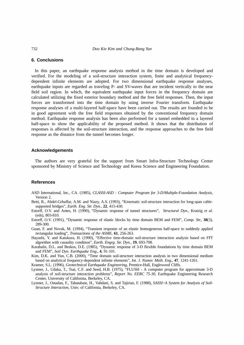
The responses along several vertical profiles of the soil are compared with the free field responsesin Fig. 11. It can be obtained that the horizontal response is affected by the soil-structure interaction,and the response approaches to those of the free field as the distance from the tunnel becomes far.In the present example, the duration of earthquakes is 40.96 sec with the step of 0.01 sec, and thetotal computational CPU time for the response of the tunnel structure in a layered soil was about 70minutes by a personal computer with 1 GHz CPU, while 45 minutes for the free field responses inSection 5.1.

Fig. 9 Comparisons of response spectra


Table 3 Ground profile of a tunnel-soil system

PropertySoil Layer

Layer Depth(m)

Mass Density(Mg/m3)

Shear Wave Velocity(m/sec)

Poisson’s Ratio

Upper layer 12.0 2.0 250 0.40Half-space ó 2.0 500 0.40

Fig. 11 Maximum horizontal acceleration of the soil medium

Fig. 10 Tunnel in an layered half-space


6. Conclusions

In this paper, an earthquake response analysis method in the time domain is developed andverified. For the modeling of a soil-structure interaction system, finite and analytical frequency-dependent infinite elements are adopted. For two dimensional earthquake response analyses,earthquake inputs are regarded as traveling P- and SV-waves that are incident vertically to the nearfield soil region. In which, the equivalent earthquake input forces in the frequency domain arecalculated utilizing the fixed exterior boundary method and the free field responses. Then, the inputforces are transformed into the time domain by using inverse Fourier transform. Earthquakeresponse analyses of a multi-layered half-space have been carried out. The results are founded to bein good agreement with the free field responses obtained by the conventional frequency domainmethod. Earthquake response analysis has been also performed for a tunnel embedded in a layeredhalf-space to show the applicability of the proposed method. It shows that the distribution ofresponses is affected by the soil-structure interaction, and the response approaches to the free fieldresponse as the distance from the tunnel becomes longer.

Acknowledgements

The authors are very grateful for the support from Smart Infra-Structure Technology Centersponsored by Ministry of Science and Technology and Korea Science and Engineering Foundation.

References

ASD International, Inc., CA. (1985), CLASSI-ASD : Computer Program for 3-D/Multiple-Foundation Analysis,Version 2.

Betti, R., Abdel-Grhaffar, A.M. and Niazy, A.S. (1993), “Kinematic soil-structure interaction for long-span cable-supported bridges”, Earth. Eng. Str. Dyn., 22, 415-430.

Estorff, O.V. and Antes, H. (1990), “Dynamic response of tunnel structures”, Structural Dyn., Kratzig et al.(eds), 803-810.

Estorff, O.V. (1991), “Dynamic response of elastic blocks by time domain BEM and FEM”, Comp. Str., 38(3),289-300.

Guan, F. and Novak, M. (1994), “Transient response of an elastic homogeneous half-space to suddenly appliedrectangular loading”, Transactions of the ASME, 61, 256-263.

Hayashi, Y. and Katukura, H. (1990), “Effective time-domain soil-structure interaction analysis based on FFTalgorithm with casaulity condition”, Earth. Engrg. Str. Dyn., 19, 693-708.

Karabalis, D.L. and Beskos, D.E. (1985), “Dynamic response of 3-D flexible foundations by time domain BEMand FEM”, Soil Dyn. Earthquake Eng., 4, 91-101.

Kim, D.K. and Yun, C.B. (2000), “Time domain soil-structure interaction analysis in two dimensional mediumbased on analytical frequency-dependent infinite elements”, Int. J. Numer. Meth. Eng., 47, 1241-1261.

Kramer, S.L. (1996), Geotechnical Earthquake Engineering, Prentice-Hall, Englewood Cliffs.Lysmer, J., Udaka, T., Tsai, C.F. and Seed, H.B. (1975), “FLUSH - A computer program for approximate 3-D

analysis of soil-structure interaction problems”, Report No. EERC 75-30, Earthquake Engineering ResearchCenter, University of California, Berkeley, CA.

Lysmer, J., Ostadan, F., Tabatabaie, H., Vahdani, S. and Tajirian, F. (1988), SASSI−A System for Analysis of Soil-Structure Interaction, Univ. of California, Berkeley, CA.


Ohsaki Research Institute (1994), “Blind prediction analysis of 1/20/94 earthquake”, Hualien LSST Meeting, PaloAlto, CA, December.

Seed, H.B. and Idriss, I.M. (1970), “Soil moduli and damping factors for dynamic response analysis”, Report No.EERC 75-29, Earthquake Engineering Research Center, University of California, Berkeley, CA.

Song, C. and Wolf, J.P. (1999), “The scaled boundary finite-element method−alias consistent infinitesimal finite-element cell method for elastodynamics”, Comput. Methods Appl. Mech. Eng., 147(3-4), 329-355.

Tzong, T.J. and Penzien, J. (1983), “Hybrid modelling of soil-structure interaction in layered media”, Rep. No.UCB/EERC-83/22, EERC, University of California, Berkeley, CA.

Wolf, J.P. (1985), Dynamic Soil-Structure Interaction, Prentice Hall.Wolf, J.P. (1988), Soil-Structure-Interaction Analysis in Time Domain, Prentice Hall.Wolf, J.P. and Song, C. (1996), Finite-Element Modelling of Unbounded Media, John Wiley & Sons.Wolf, J.P. and Obernhuber, P. (1982), “Free field response from inclined SH-waves and Love-waves”, Earthq.

Eng. Str. Dyn., 10, 823-845.Yun, C.B., Kim, D.K. and Kim, J.M. (2000), “Analytical frequency-dependent infinite elements for soil-structure

interaction analysis in two-dimensional medium”, Engineering Structures, 22(3), 258-271.Zhang, C. and Zhao, C. (1988), “Effects of canyon topography and geological condition on strong ground

motion”, Earth. Eng. Str. Dyn., 16, 81-97.Zhang, X., Wegner, J.L. and Haddow, J.B. (1999), “Three-dimensional dynamic soil-structure interaction analysis

in time domain”, Earth. Engrg. Str. Dyn., 28(12), 1501-1524.Zhao, C. and Valliappan, S. (1993), “An efficient wave input procedure for infinite media”, Communications in

Numerical Methods in Engineering, 9, 407-415.

Documents

Time domain earthquake response analysis method for 2-D ...ssu.ac.ir/cms/fileadmin/user_upload/Moavenatha/Mposhtibani/Mdaftar... · Time domain earthquake response analysis method