Time Eï¬ƒcient Solution of Phase Equilibria in Dynamic and

Time Efficient Solution of Phase Equilibria in Dynamic andDistributed Systems with Differential Algebraic Equation SolversØivind Wilhelmsen,*,†,‡ Geir Skaugen,† Morten Hammer,† Per Eilif Wahl,† and John Christian Morud§

†SINTEF Energy Research, N-7465 Trondheim, Norway‡Department of Chemistry, Norwegian University of Science and Technology, N-7491 Trondheim, Norway§SINTEF Materials and Chemistry, N-7465 Trondheim, Norway

*S Supporting Information

ABSTRACT: Solution of phase equilibria with flash calculations is central in many processes. During the integrating of theconservation equations in these systems, flash calculations are traditionally solved in inner loops at each integration step. Some ofthese systems can be solved more efficiently using modern DAE solvers, where the differential equations and the algebraicequations describing the phase equilibrium are solved simultaneously. In this paper we present a framework, called theThermodynamic Differential Algebraic Equation (TDAE) method, which handles most two-phase flash variants. The phaseboundary is tracked, enabling a robust solution also with phase changes. The time consumption of the TDAE method has beencompared to the traditional approach in several examples implemented in both Fortran and Matlab. In some cases, the TDAEmethod is more than 800 times faster, and in other cases the traditional methodology should be used. We will give insight intohow and when DAE solvers can be used to speed up phase equilibrium calculations.

1. INTRODUCTION

Solving the phase equilibrium between coexisting phases, alsocalled flash calculations, has been discussed much in the lastdecades. It still represents a challenge, in particular for systemswhere temperatures and pressures are not specified. There is alarge variety of processes where flash calculations are important,such as multiphase transport of fluids in pipelines, heatexchangers, distillation columns, separation units, and chemicalreactors. Robust flash calculations are demanding, in particularnear the critical point, and they are often the bottleneck forspeedup of calculation time. Hillestad et al. claims that inflowsheet simulations, 70−90% of the computational time isspent on calculation of thermodynamic properties.1 The mostcommon flash is the Temperature, Pressure (TP-flash), wheretemperature, pressure, and overall composition is specified andcomposition of gas/liquid and the vapor fraction are unknownvariables. Before 1980, the governing method to solve the TP-flash was the K-value method, also known as the Rachford−Rice method.2−4 The K-value method is still used in processsimulations but is often accelerated by dominant eigenvaluemethods and followed by a second order Newton−Raphsonapproach.3−6

Different models will require the phase equilibrium to besolved with different specifications. Modeling of multiphaseheat exchangers often requires a flash where enthalpy andpressure is specified (HP-flash), while transient simulations ofmultiphase flow in pipelines may require a flash with specifiedinternal energy and volume (UV-flash). These flash calculationsare in general harder to solve and less robust than the TP-flash.Giljarhus Teigen et al. has for instance described the solution ofthe UV-flash as one of the main challenges in modeling ofpipeline transport of CO2 with accurate equations of state.7

The most common approach to solve systems with phaseequilibria is to perform the calculations in inner loops,

separated from the higher-level modeling. This method willbe referred to as the traditional methodology in the rest of thiswork. The advantage is that algorithms tailored for robust flashcalculations can be applied. A disadvantage is that the approachleads to nested iterations loops. Numerical noise is when thefluctuations of internal variables due to limited accuracy arecomparable to the predefined solution tolerance, which can givean unstable solution. To avoid numerical noise, the flashcalculations must be solved to an order of magnitude tighterthan the tolerance of the higher level modeling. This willincrease the computational time. Methods to speed up flashcalculation have been suggested by several authors in theliterature. The shadow region method proposed by Michelsenand Mollerup reduces the computational time by assemblingknowledge of how close a point is to the two-phase regionthrough the identification of a shadow region. The shadowregion is the points in the single phase region where a nontrivialpositive minimum of the tangent plan distance exists.4 Inaddition, the stability analysis for a large portion of the points inthe single phase region can be skipped if they are outside theshadow region, and decent initial values from previousiterations may be used to speed up calculations.4 Rasmussenet al. have shown that for transient pipeline simulations, thecomputational time can be reduced by 85−90% using thismethod.8 Another alternative to speed up thermodynamiccalculations is table-lookup routines. The compositional spaceadaptive tabulation method saves computation time byreplacing some of the phase split calculations in the two-phase region with prestored flash calculation results and is

Received: September 24, 2012Revised: December 28, 2012Accepted: January 6, 2013Published: January 8, 2013

Article

pubs.acs.org/IECR

© 2013 American Chemical Society 2130 dx.doi.org/10.1021/ie302579w | Ind. Eng. Chem. Res. 2013, 52, 2130−2140

pubs.acs.org/IECR

essentially a sophisticated table look-up framework.9 Tablelook-up routines have also been used to speed up calculationswith the reference equation of state for CO2 by Andresen andSkaugen.10 Tables often become large and unpractical for two-phase multicomponent mixtures.In this work, we will demonstrate how to use a framework

which takes advantage of modern Differential AlgebraicEquation (DAE) solvers to solve the two-phase equilibriumbetween gas and liquid more time efficiently. The increase incomputational time for flash calculations in inner loops such asin the traditional methodology and the shadow region methodand the loss in accuracy in table look-up is avoided in thisapproach. In addition, the approach is fast to implement, and itis trivial to change the flash specifications. With DAE solvers,the algebraic equations defining the phase-equilibrium equationsystem can be solved with the same accuracy as the differentialequations representing the dynamic or distributed system, andprevious iterations are automatically used as initial values forthe next.It is a well-established idea to add the algebraic equations

defining the phase equilibrium to the conservation equations ina DAE formulation, used by several authors in the literature.Pingaud, for instance, formulated a multiphase heat exchangermodel as a DAE system already in 1989.11 Phase equilibrium indistillation columns has been formulated as DAE problems byseveral authors, for instance.12−15 Flash drums have recentlybeen solved with modern DAE solvers by Goncalves et al.16 andLima et al.17 Common for all these cases is that the system isalways in the two-phase region, and the challenge of crossingthe phase boundary is avoided. The chemical and phasebehavior in reservoir processes was formulated as a DAEproblem by Kristensen et al.,18 where they also showed howphase changes can be handled with event functions in DAEsolvers. Additional difficulties are associated with the simulationof LNG heat exchangers, since they may operate with thenatural gas above the critical pressure, and several phasetransitions are possible. With large variations in thethermophysical properties, rapid phase changes, and disconti-nuities near the phase boundaries, these heat exchangersrepresent a challenge for robust simulations.19 To use DAEsolvers as a general tool for flash calculations comparable to thetraditional approach requires a framework which can

• Handle the most common flash specifications• Work both in the single-phase and two-phase area• Keep track of the states of the system and handle phase

boundaries robustly• Work above and near the critical point

Such a framework has currently not been presented in theopen literature. This leaves DAE solvers as a tool for thespecific cases away from single-phase boundaries, such asdistillation columns, flash-drums, etc., and the traditionalapproach is the only alternative for the general case. We willpropose a framework in Section 2 aiming to handle therequirements above, which will be referred to as theThermodynamic Differential Algebraic Equation (TDAEmethod). We will show how it can be extended to supercriticalpressures in Section 2.4 and will describe how it can beimplemented in Fortran, C, and Matlab in Section 2.5. With theTDAE method at hand we will investigate for which models,cases, and implementations DAE solvers can be used to speedup flash calculations compared to the traditional approach. Thisquestion has not yet been addressed in the open literature. The

main cases will be described in Section 3, namely, the dynamicdepressurization of a tank involving the solution of a UV-flashand a multistream LNG heat exchanger where a HP-flash isnecessary. Results will be presented and discussed in Section 4,and concluding remarks can be found in Section 5.

2. THEORYIn this section, we will describe a framework for DAE solverswith simultaneous solution of the conservation equations andthe equations describing the phase equilibrium. The frameworkhas been called the thermodynamic differential algebraicequation (TDAE) method. In addition to a robust DAE solver,a thermodynamic package, library, or implementation must beavailable. Variables such as K values, enthalpies, entropies, andvolumes must be supplied as functions of temperatures,pressures, and compositions. Modeling of macroscopic systemsoften means specification of the differential equationsdescribing conservation of mass, energy, and momentum,which typically are20

ρ ρ

ρ ρ

ρ ρ

∂∂

+ ∇· =

∂∂

+ ∇· =

∂∂

+ ∇· + ∇ =

tv

et

ve f

vt

vv P f

( ) 0 continuity

( )( ) energy

( )( ) momentum

e

z (1)

Here, ρ is the mass density, t is the time, v is the velocity, e isan energy variable, and fe, fz are energy and momentum sourceterms. The energy conservation may be formulated withinternal energy, enthalpy, entropy, or temperature as thegoverning variable. We call each system with one equation foreach of the conserved variables a subsystem. The differentialequations and variables which are found either necessary orconvenient to fully describe the system will affect thespecification of the flash calculations. Consider for instancedynamic simulations where the mass flow varies with time andthe energy conservation is formulated with the internal energy.If equilibrium between the phases is assumed, temperatures andpressures are not specified but are available through thesolution of an UV-flash. This formulation is, for instance,central in two-phase modeling of shock wave propagation inpipelines.7,21,22 In typical steady state modeling of multi-component heat exchangers with phase change, the massbalance is trivial, the energy balance is formulated in theenthalpy, and the momentum balance reduces to a differentialequation in pressure.23,24 Here, a HP-flash is necessary tospecify temperature and composition of the coexisting phases.In other applications, the differential equation might be in thetemperature, and the traditional TP-flash is sufficient. TheTDAE method can handle all these cases. In addition, themethod gives DAE systems of index-1 which can be solved bymost DAE solvers.25 The framework may be setup according tothe following steps:

1. Define the state vector for each subsystem consisting ofthe variables of the differential equations and thealgebraic variables corresponding to the specified flashcalculations.

2. Implement the differential and algebraic equationscorresponding to the state vector in a DAE solver. Theimplementation may be divided into the following parts:

Industrial & Engineering Chemistry Research Article

dx.doi.org/10.1021/ie302579w | Ind. Eng. Chem. Res. 2013, 52, 2130−21402131

(a) Calls to a thermodynamic routine and calculationof variables based on values from the state vector.

(b) Calculation of the residuals corresponding to thealgebraic variables of the state vector.

(c) Handling phase changes.

2.1. Defining the State Vector of Each Subsystem. Asexplained previously, different conservation equation formula-tions require their specific flash calculations and hence differentstate vectors and residuals. In this work, four classes of statevectors are used for each subsystem depending on the flashspecifications:

=v T K wT P[ , , , , ]1 inc inc (2)

=v T K w TE P[ , , , , , ]2 inc inc (3)

ρ= v T K w PT[ , , , , , ]3 inc inc (4)

ρ= v T K w T PE[ , , , , , , ]4 inc inc (5)

Here, bold denotes the main variables of the differentialequations. The remaining variables are connected to thealgebraic equations which can be formulated as residuals. Thephase boundaries of the two-phase region, also called bubbleand dew points, are tracked using an incipient temperature, Tinc,which may be understood as

=

‐

‐

‐

⎧⎨⎪⎪

⎩⎪⎪

T

T

T

T

single phase liquid (bubble point)

single phase gas (dew point)

two phase gas/liquidinc

bub

dew

Furthermore, the incipient K-value, Kinc, is the K-value at theincipient temperature, P is the pressure, and y and x thecompositions in gas and liquid. Kinc represents the equilibriumvariable for a two-phase mixture and the variable associatedwith bubble and dew points in a single-phase mixture. w is thevapor fraction and ρ is the molar density. The least number ofalgebraic equations is needed in the TP-flash, where differentialequations for the temperature and pressure evolutions aregiven. Here, a TP-flash may be necessary in the two-phaseregion, and the state vector in the TDAE method should be v1defined in eq 2. In cases where the momentum balance isrepresented by a differential equation in pressure and theenergy balance is formulated in the energy variable, E,representing either the enthalpy, H, the entropy, S, or theinternal energy, U, of the system, the governing flash is eitheran HP-, SP-, or UP-flash. For the EP-flash, the state vector willbe given by v2 in eq 3. In dynamic modeling where mass flowvaries, the pressure may be given implicitly if phase equilibriumis assumed. If the energy balance is formulated in thetemperature, the flash calculation performed will be a TV-flash and the state vector is v3 given by eq 4. In dynamic caseswhere the mass flow changes and the energy is defined with anenergy variable, the flash calculations will be a SV-, UV-, or HV-flash and the state vector is v4 given by eq 5.2.2. Calculations. 2.2.1. State Variable and Calls to the

Thermodynamic Package. This section defines the inter-mediate calculations and calls to the thermodynamic package.Using the algebraic variables from the state vector, thecompositions in the liquid phase, x, can be calculated:

=

‐

‐

+ − ‐

⎧

⎨⎪⎪

⎩⎪⎪

x

z

z K

z w K

(a) single phase liquid

/ (b) single phase gas

/(1 ( 1)) (c) two phase gas/liquid

inc

inc

(6)

Here, z is the overall composition. Notice that the equationsare different for single-phase liquid, single-phase gas, and two-phase gas and liquid (eq 6a,b,c). In the two-phase area, theexpression is a variant of the Rachford Rice equation.2−4 Thecomposition in the vapor phase, y, is then

=y K xinc (7)

Furthermore, a new incipient K-value can be calculated:

=K K T P x y( , , , )inc,c c inc (8)

Subscript c denotes variables which are obtained from athermodynamic package. If the energy is defined through E,which may be enthalpy, internal energy, or entropy, thefollowing calculations are necessary:

=

=

E E T P x

E E T P y

( , , )

( , , )

c c

c c

liq,

gas, (9)

=

‐

‐

− + ‐

⎧

⎨⎪⎪⎪

⎩⎪⎪⎪

E

E

E

w E wE


(b) single phase gas

(1 ) (c) two phase gas/liquid

c

liq,c

gas,c

liq,c gas,c

(10)

If the density is given by the continuity equation and thepressure is given implicitly, the molar volume must becalculated:

=

=

V V T P x

V V T P y

( , , )

( , , )

liq,c c

gas,c c (11)

=

‐

‐

− + ‐

⎧

⎨⎪⎪⎪

⎩⎪⎪⎪

V

V

V

w V wV


(b) single phase gas

(1 ) (c) two phase gas/liquid

c

liq,c

gas,c

liq,c gas,c

(12)

2.2.2. Residuals of the Algebraic Variables. The algebraicvariables in the state vectors v1−v4 in eqs 2−4 require theircorresponding residuals, which will be below a predefinedtolerance in the final solution. To ensure that the mole fractionsin the gas and liquid are normalized, the residual chosen for Tincis

∑= −x y0 ( )k

k k(13)

The residuals of the incipient K-values, Kinc, are given by

= −K K0 inc,c inc (14)

The residual of the vapor fraction, w, depends on the phase



=

‐

− ‐

− ‐

⎧⎨⎪⎪

⎩⎪⎪

w

w

T T

0


1 (b) single phase gas

(c) two phase gas/liquidinc (15)

If the temperature is given implicitly, the residual of E is (v2 andv4)

= − EE0 c (16)

In cases where the pressure is implicit, the residual of P is (v3and v4)

ρ= −V

01

c (17)

2.2.3. Handling of Phase Changes. In the TDAE method,the phase boundary is tracked in the single-phase region toenable a robust handling of phase transitions. Since thealgebraic equations in the previous sections change in a phasetransition, it is necessary to locate these events. This may behandled by an event detection routine in the DAE solver, whichstops the integrator when the following roots are found:

=

− ‐‐

− ‐‐

⎧

⎨⎪⎪

⎩⎪⎪

w w

T T0

(1 ) for changes from two phase to single phase

for changes from single phase to two phase

inc

(18)

2.3. Summary of the Equations. The equations to use ineach subsystem depend on the specifications of the flash andare summarized in Table 1. In addition, equations denoted (a)will be used in the liquid-phase, (b) in the gas-phase, and (c) intwo-phase gas and liquid.

2.4. Extension of the TDAE Method to SupercriticalPressures. The incipient temperature described in theprevious section is used to track the phase boundary. In thesingle-phase region, the incipient state can be interpreted as thebubble or dew point temperature at a specified pressure. Thestate is thus ambiguous for pressures above the critical pressureand undefined above the cricondenbar.An alternative is to redefine the incipient state to the

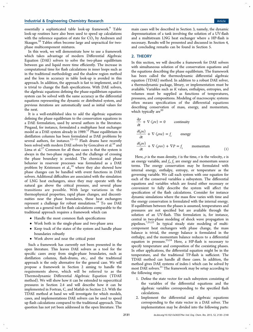
temperature and pressure on the phase boundary at a linesegment between the actual pressure and temperature (T, P)and a reference state inside the two-phase area as shown inFigure 1. With this incipient state, the phase boundary can betracked given that the reference point is always in the two-phasearea. A complicating factor is that the incipient state maychange from being a bubble point (blue line in Figure 1) to adew point (red line in Figure 1), without a change in theequations according to the formulation in the previous section.From a computational point of view, it is difficult to solve theRachford−Rice equations in the vicinity of the critical point,

and the system of equations used to track the incipient statewill be close to singular. This can be solved by introducing asecond reference point in the two-phase area, which will bereferred to as the extended TDAE method. Consider forinstance the situation where the (T, P)-state in Figure 1 movesto the left. First, the reference point (Trg, Prg) can be used, andthe incipient state is a dew point. When the incipient statereaches a safety boundary around the critical point, (Tcrit), anevent function stops the integrator and changes the referencestate to (Trl, Prl), and the equations can here be changed suchthat the incipient state represents a bubble point. From acomputational point of view, the incipient temperature in thestate vector can be exchanged with the following iterationvariable, θ, which gives a new incipient state (Tinc2, Pinc2)defined as

θ θ

θ θ

= + −

= + −

T T T

P P P

(1 )

(1 )

inc2 ref

inc2 ref (19)

Calculations and residuals in the TDAE method are the sameas in the previous section, except the residual of the vaporfraction, which should be changed to

θ

=

‐

− ‐

− ‐

⎧⎨⎪⎪

⎩⎪⎪

w

w0


1 (b) single phase gas

1 (c) two phase gas/liquid (20)

The incipient pressure, Pinc2, also has to be included in thecalculation of the incipient K-value. One more event functionshould be introduced and used if some of the pressures areexpected to be above the critical pressure. This event functionrepresents the place where a change in reference state occurs:

ε= | − | −T T0 inc2 crit (21)

Here, subscript crit denotes the critical state. The variable ε isintroduced to avoid calculations near the critical point. Thereference pressure and temperature will be given by (Trg, Prg) ifthe incipient state is in the gas-phase area and (Trl, Prl) if thestate is in the liquid-phase area. If these two reference states arechosen close to their respective phase boundaries and the ε-limit is chosen small enough, the algorithm will be able to

Table 1. Summary of the Equations Used in the TDAEMethod

flash specs

T-P U/S/H-P U/S/H-ρ

state vector eq 2 eq 3 eq 5calculations eqs 6−8 eqs 6−10 eqs 6−12residuals eqs 13−20 eqs 13−16 eqs 13−17

Figure 1. TDAE method modified to account for supercriticalpressures using two reference points, one near the bubble points, (Trl,Prl) and one near the dew-points, (Trg, Prg). The phase envelopebelongs to natural gas showing bubble points (left line) and dewpoints (right line).



handle all regions at some distance from the critical point, sincethe incipient state avoids the critical point by changingreference state as the ε-limit is reached (see Figure 1). Thereference points should be chosen such that a transition fromone to the other involves a change in the incipient temperaturewhich is larger than the ε-limit around the critical point.2.5. How to Computationally Implement the Frame-

work. During the 1980s and 1990s, DAE methods becamepopular in many scientific fields and received much attention.Modern DAE solvers may be divided in two categoriesaccording to how they are solved: multistep and single-stepmethods. In multistep methods, information from severalprevious steps is used in prediction of the next. Methods basedon the backward differentiation formula and the numericaldifferentiation formula are popular. Examples are the DASSL25

code and decedents (e.g., DASKR, SDASRT, DASPK,IDA).26−28 Typically, multistep methods start with a lowerorder of accuracy and small steps and build up to higher orderas more information is available,25 thus making the multistepmethodology preferred in most cases. Single-step methods useonly information from the previous step to evaluate the next.For cases with discontinuities, such as several phase transitions,where the solver must be stopped and restarted, they havepotential advantages over multistep methods. Variations ofimplicit Runge−Kutta methods are popular single-stepmethods, such as the code RADAU by Hairer and Wanner29

and PSIDE by De Swart et al.30 A thorough treatment of DAEmethods can be found in the books by Hairer and Wanner andBrenan et al.25,29 In the implementation of the TDAE method,the integration should be stopped at the location of an eventdefining the phase transition. Many solvers fail as thesediscontinuities are encountered, but some manage to continuethe integration. Integration across these discontinuities,however, may lead to nonphysical results, step failures, andtrouble with a robust solution.18 Most of the solvers mentionedabove are available in Fortran (for instance, DASKR, DASSL,SDASRT) and some are written in C (IDA). The TDAEmethod may also be implemented in Matlab with the routinesfor initial value problems, ode15s or ode23t with a singularmass matrix. Alternatively, the fully implicit solver ode15i maybe used. Event functions are easily accessible in Matlab and canbe used to locate phase transitions. Either the thermodynamicfunctions may be programmed directly in Matlab, obtainedthrough commercial programs such as Refrop from NIST,31 orMex-files can be created from thermodynamic packages in C,Fortran, or other languages.

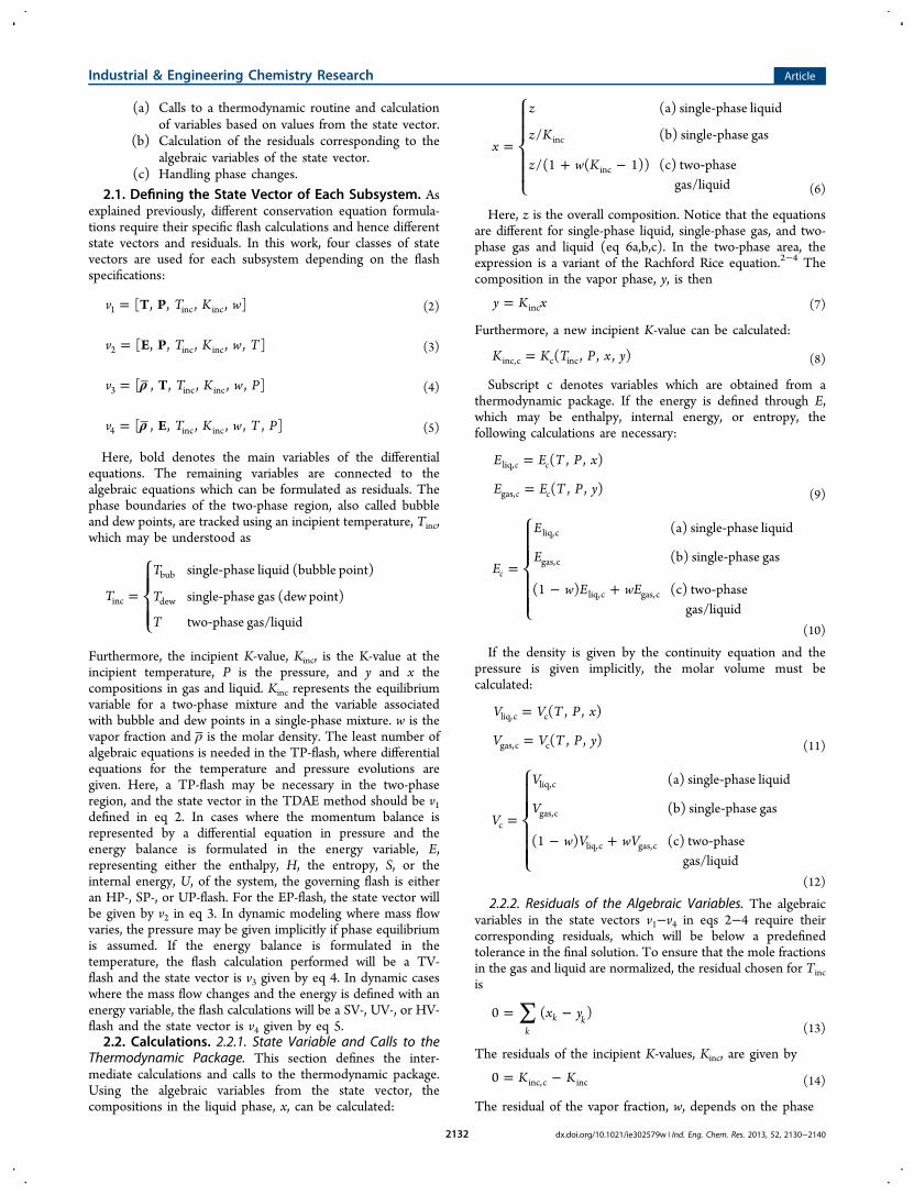
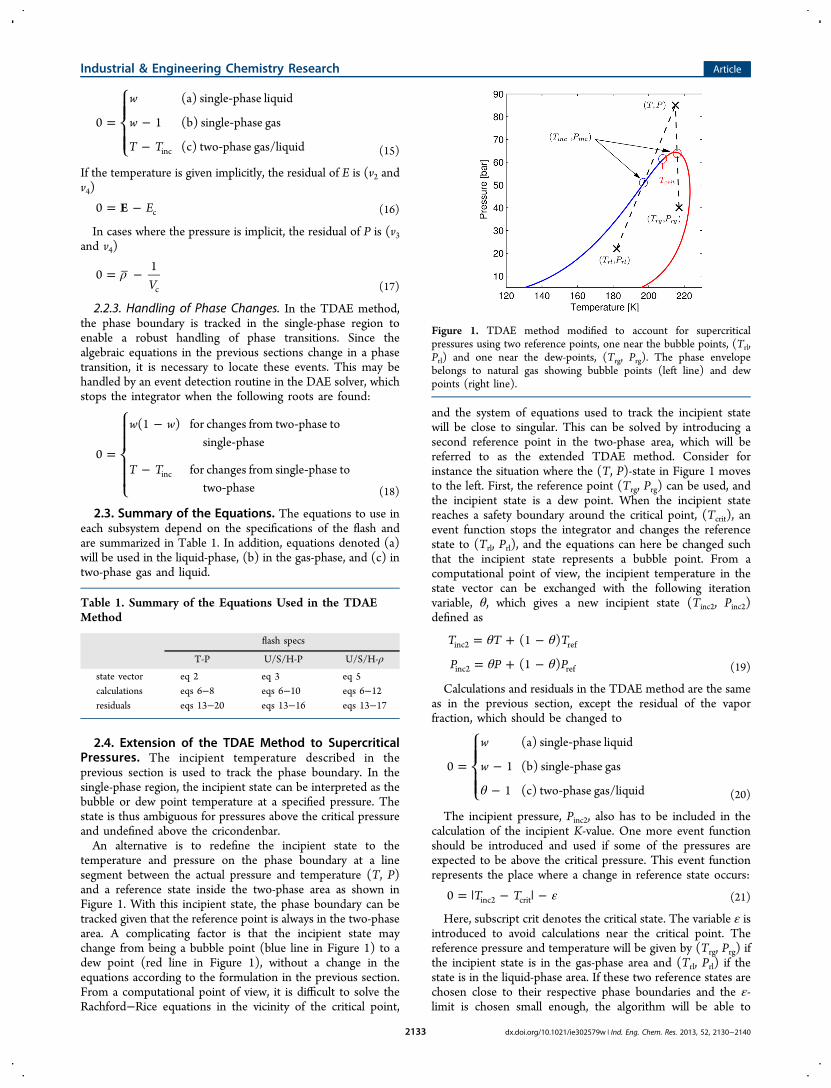
3. DEMONSTRATION CASESThe comparison of using DAE solvers or the traditionalapproach for flash calculations will be made for two mainsystems where flash calculations are central parts of the solutionprocess, one distributed and one dynamic. The first case is thedynamic depressurization of a tank containing both gas andliquid (Figure 2). The second case is the steady state solution ofa distributed multistream heat exchanger for liquefaction ofnatural gas (Figure 3). All cases were solved with absolute andrelative tolerances of 10−5. In Fortran, the routine DASKR,available at the Netlib webpage, was used.26,27 Some of thecases were also implemented in Matlab to compare computa-tional implementations. Here the routine ode23t was used. Thecubic equation of state, Soave−Redlich−Kwong, was used in allcases.32−34 In principle, any equation of state capable of vapor−liquid equilibrium calculations could be used.35

3.1. Depressurization of a Tank. The first main case isthe depressurization of a tank, which is a multicomponentanalogue to the case recently addressed by Giljarhus Teigen etal.7 Consider a tank containing mixed refrigerant at 298 K and5.5 MPa. With these conditions, there will be both gas andliquid inside the tank. At time = 0, a valve at the bottom of thetank is opened, and fluid flows out in the ambient. If thetemperature in the tank becomes too low, the material mightbecome brittle. We would thus like to predict the minimumtemperature in the tank during this event. The mass,component, and energy balances of the tank are7,20

ρ ρ∂ ∂

= − Vt

m T( , )t (22)

Figure 2. Illustration of the tank in the dynamic depressurization case.

Figure 3. Illustration of the heat exchanger case. Here NG refers tonatural gas and MR is mixed refrigerant.



ρρ ρ

∂ ∂

= − ∀Vt

m T i( , , )ii it (23)

ρ ρ ρ∂ ∂

= − VUt

Q m T h T( )

( , ) ( , )t t t (24)

Here, Vt is the volume of the tank, m is the molar flow, T isthe temperature, U is the internal energy, Qt is the heattransferred, ht is the enthalpy of the outlet stream, and t is thetime. The flow rate out of the tank is given by a standard valveequation, the heat flow specified by an overall heat transfercoefficient, and the temperature difference between the tankand the ambient. It is assumed that liquid and gas are inequilibrium at all times, which means that the composition ofthe fluid leaving the tank equals the composition of theequilibrated liquid except when the mixture is one-phase gas.Specific model parameters like composition of the mixedrefrigerant and geometry of the tank is given in Appendix Alocated in the Supporting Information. Since the heattransferred to the tank depends on the temperature differenceand the mass leaving the tank affects the overall composition,UV-flash calculations are necessary to solve this problem. TheUV-flash will be handled with the TDAE method in one case,which will be compared to a state-of-the-art UV-flash solved viaa combination of a nested loop and a direct Newton−Raphsonalgorithm representing the traditional method. The Newton−Raphson approach uses the initial values from the previousiteration in the first attempt to solve the UV-flash. If it fails, theslower but more robust nested-loop routine is used. Details aregiven in Appendix B located in the Supporting Information.3.2. Multistream LNG Heat Exchanger. Mathematical

models of a counter-current LNG heat exchanger is the secondmain case. The geometry is modeled as two tubes in a shell(Figure 3). In practice, the shell will contain several tubes andthe equations below are formulated for an arbitrary number, nt.The configuration in Figure 3 is, however, sufficientlycomplicated for the investigations in this work. Natural gasand mixed refrigerant at high pressures is liquefied in the twotubes by mixed refrigerant at lower pressures evaporating incounter-current flow on the shell side. Steady state energybalances in the shell and the tubes are

∑π∂∂

= ≠

Hl m

D Jj

j js

s s

nt

q,(25)

π∂∂

= −

H

l

D J

mj j q j

j

,

(26)

Here, H denotes the enthalpy, D the outer diameter, Jq theheat flux, and l the spatial dimension in the heat exchanger, andthe subcripts s and j refer to the shell and tube j, respectively.Moreover, the momentum balances of the shell and tubessimplify to differential equations in the pressure:

ρρ β

∂∂

= −Pl

fm

A Dg

2sin( )s

ss

2

s2

s h,ss

(27)

ρρ β

∂∂

= − −P

lf

m

A Dg

2sin( )j

jj

j j jt

2

2(28)

Here, P is the pressure, f is the friction factor, m is the massflow rate, A is the cross section area, ρ is the density, g is thegravity constant, and β is the angle between the l-axis and the

horizontal axis. Since the heat transfer between the tubes andthe shell is a function of the temperatures, it is necessary toperform flash calculations with specified enthalpy and pressure(HP-flash). Both heat transfer and pressure drop depend onwhether boiling/condensation occurs or if the fluids are single-phase. Moreover, the mechanisms for transfer of energy andmomentum depend on whether the flow is laminar orturbulent. To take into account the changing conditions inthe heat exchanger, heat transfer coefficients and friction factorsbased on empirical expressions have been used for some of thesubcases.In the case of nonconstant heat transfer coefficients, the

overall heat transfer coefficient for tube j, αtot,j is needed:

α α λ α= + +

D D D D

D1 1 ln( / )

2j j

j i j j

j

j

j jtot,

,

,in ,in (29)

Here, subscript in refers to the inner tube wall, αj is the outerheat transfer coefficient for tube j, αj,in is the inner heat transfercoefficient, and kw,j is the thermal conductivity of the tubewall.On the basis of a steady-state energy balance across the tubewall, the outer wall temperature can be calculated:

α

α= − −T T T T( )j

j

jjw ,c s

tot,s

(30)

The wall temperatures Twj were obtained by solving algebraicequations at each integration step:

= − ∀T T j0 j jw w ,c (31)

The heat exchanger was integrated in the positive l-directionat each iteration with a negative sign on the shell streamflowrate. The counter-current heat exchanger problem was solvedby iterating on the outlet temperature and pressure of the shellstream using a steepest descent search. Relaxation factors wereused to ensure a smooth approach to the final solution. Themost robust solution methodology was achieved by updatingthe inlet pressure of the shell stream when the relative error inthe inlet temperature was less than 10−4. Like the UV flash, theHP flash gives an entropy maximization problem for thetraditional approach. Details are given in Appendix B located inthe Supporting Information. To elucidate important propertiesand limitations of the TDAE method, three subcases will bediscussed, sHX, cHX. and HX.sHX: This case is the simple heat exchanger (sHX), where

constant heat transfer coefficients and friction factors are used.These simulations represent the cases where the flashcalculations are responsible for most of the computational time.cHX: The case is identical to sHX, except that the natural gas

has an inlet pressure of 8 MPa, which is above the criticalpressure (6.2 MPa). The extended TDAE method from Section2.4 is tested for this case.HX: This is the most complex case, where empirical

expressions are used to model heat transfer coefficients andfriction factors. The empirical relations require thermophysicalproperties in addition to the flash calculations. Since some ofthe heat transfer coefficient correlations are functions of thewall temperatures and the wall temperatures are functions ofthe heat transfer coefficients, additional calculations andresiduals are associated with the wall temperatures in this case.The same thermodynamic library was used in all the cases.

This library was used as a statically linked library file in theFortran implementation. In Matlab, the construction of Matlab



Executable (MEX)-files was necessary to make the routinesavailable. A MEX-file provides an interface between Matlab andsubroutines written in C, C++, or Fortran. When compiled,they are dynamically loaded and allow Fortran code to beinvoked from within Matlab as if it was a built-in function.Other thermodynamic libraries, such as Refprop,31 are alsoavailable for Matlab through MEX-files. Each call andinitialization of a MEX-file represents a loss in computationaltime compared to a pure Fortran application. Two differentMatlab implementations have thus been compared. In MEX1, acompact MEX-file was created and all necessary thermophysicalproperties of a stream were obtained with a single call usingtemperature, pressure, and vapor/liquid compositions as inletvariables. In MEX2, each calculation of a thermophysicalproperty represented a separate call to the MEX-file. This ismost likely the only alternative if a thermodynamic package iscalled as a “black-box”. Geometries, inlet temperatures,pressures, and composition for the cases are given in AppendixA found in the Supporting Information.

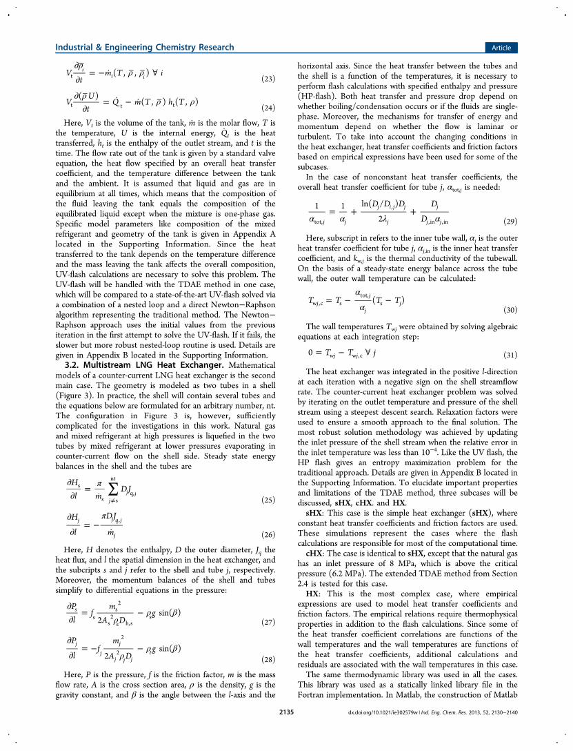
4. RESULTS AND DISCUSSIONAll cases were successfully solved within the predefinedaccuracy, and no difference in robustness was observed betweenthe TDAE method and the traditional methodology. Figure 4

shows how the vapor-fraction and temperature in the tanksimulation change with time. The figure shows that the tankcontains only gas after t ≈ 650 s at which the tank temperatureis at its minimum. The tank simulation involves one phasechange, from two-phase gas/liquid to single-phase gas.In the main case of the multistream LNG heat exchanger,

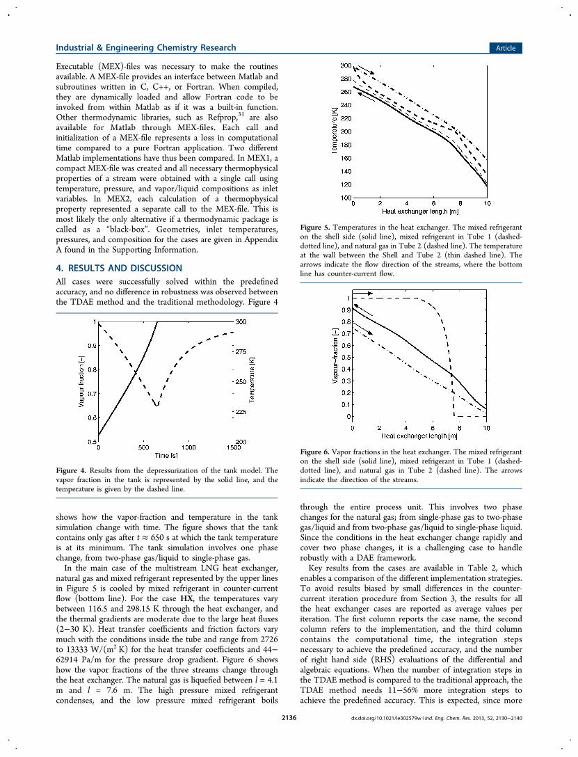
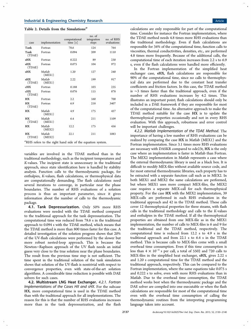
natural gas and mixed refrigerant represented by the upper linesin Figure 5 is cooled by mixed refrigerant in counter-currentflow (bottom line). For the case HX, the temperatures varybetween 116.5 and 298.15 K through the heat exchanger, andthe thermal gradients are moderate due to the large heat fluxes(2−30 K). Heat transfer coefficients and friction factors varymuch with the conditions inside the tube and range from 2726to 13333 W/(m2 K) for the heat transfer coefficients and 44−62914 Pa/m for the pressure drop gradient. Figure 6 showshow the vapor fractions of the three streams change throughthe heat exchanger. The natural gas is liquefied between l = 4.1m and l = 7.6 m. The high pressure mixed refrigerantcondenses, and the low pressure mixed refrigerant boils

through the entire process unit. This involves two phasechanges for the natural gas; from single-phase gas to two-phasegas/liquid and from two-phase gas/liquid to single-phase liquid.Since the conditions in the heat exchanger change rapidly andcover two phase changes, it is a challenging case to handlerobustly with a DAE framework.Key results from the cases are available in Table 2, which

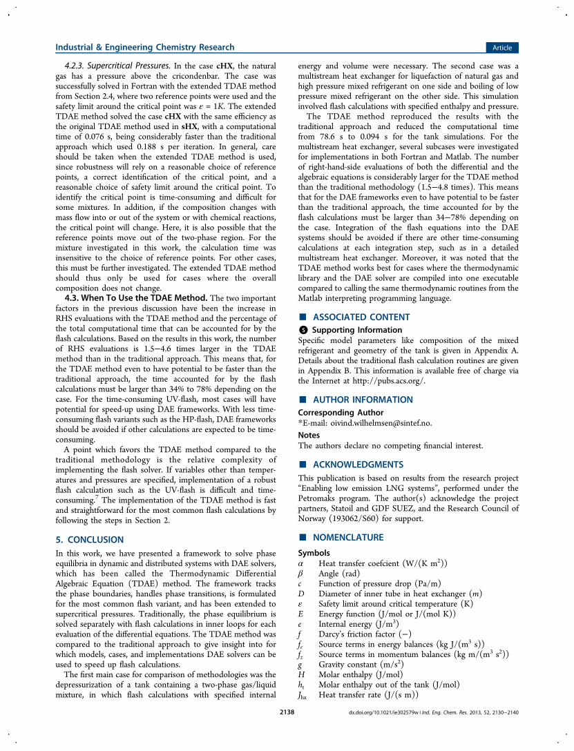
enables a comparison of the different implementation strategies.To avoid results biased by small differences in the counter-current iteration procedure from Section 3, the results for allthe heat exchanger cases are reported as average values periteration. The first column reports the case name, the secondcolumn refers to the implementation, and the third columncontains the computational time, the integration stepsnecessary to achieve the predefined accuracy, and the numberof right hand side (RHS) evaluations of the differential andalgebraic equations. When the number of integration steps inthe TDAE method is compared to the traditional approach, theTDAE method needs 11−56% more integration steps toachieve the predefined accuracy. This is expected, since more

Figure 4. Results from the depressurization of the tank model. Thevapor fraction in the tank is represented by the solid line, and thetemperature is given by the dashed line.

Figure 5. Temperatures in the heat exchanger. The mixed refrigeranton the shell side (solid line), mixed refrigerant in Tube 1 (dashed-dotted line), and natural gas in Tube 2 (dashed line). The temperatureat the wall between the Shell and Tube 2 (thin dashed line). Thearrows indicate the flow direction of the streams, where the bottomline has counter-current flow.

Figure 6. Vapor fractions in the heat exchanger. The mixed refrigeranton the shell side (solid line), mixed refrigerant in Tube 1 (dashed-dotted line), and natural gas in Tube 2 (dashed line). The arrowsindicate the direction of the streams.



variables are involved in the TDAE method than in thetraditional methodology, such as the incipient temperatures andK-values. The incipient state is unnecessary in the traditionalapproach, since state identification here is handled by stabilityanalysis. Function calls to the thermodynamic package, forenthalpies, K-values, flash calculations, or thermophysical dataare computationally demanding. The flash calculations needseveral iterations to converge, in particular near the phaseboundaries. The number of RHS evaluations of a solutionprocess is thus an important parameter, since it givesinformation about the number of calls to the thermodyamicpackage.4.1. Tank Depressurization. Only 50% more RHS

evaluations were needed with the TDAE method comparedto the traditional approach for the tank depressurization. Thecomputational time was reduced from 78.6 s in the traditionalapproach to 0.094 s with the TDAE method, which means thatthe TDAE method is more than 800 times faster for this case. Adetailed investigation of the solution progress shows that 20%of the UV-flash calculations were performed by the slower butmore robust nested-loop approach. This is because theNewton−Raphson approach of the UV flash needs an initialguess very close to the true solution near the phase boundaries.The result from the previous time step is not sufficient. Thetime spent in the traditional solution of the tank simulationshows that solution of the UV-flash is nontrivial with respect toconvergence properties, even with state-of-the-art solutionalgorithms. A considerable time reduction is possible with DAEsolvers for such cases.4.2. Multistream LNG Heat Exchanger. 4.2.1. Fortran

Implementations of the Cases HX and sHX. For the subcaseHX, more computational time is used in the TDAE methodthan with the traditional approach for all implementations. Thereason for this is that the number of RHS evaluations increasesmore than in the tank depressurization, and the flash

calculations are only responsible for part of the computationaltime. Consider for instance the Fortran implementation, wherethe TDAE method needs 4.8 times more RHS evaluations thanthe traditional methodology. Even if flash calculations areresponsible for 34% of the computational time, function calls toviscosities, thermal conductivities, densities, etc., are performed4.8 times more frequently. Because of the additional calls, thecomputational time of each iteration increases from 2.2 s to 6.9s, even if the flash calculations were handled more efficiently.In the Fortran implementation of the simplified heat

exchanger case, sHX, flash calculations are responsible for90% of the computational time, since no calls to thermophys-ical data are performed due to the constant heat transfercoefficients and friction factors. In this case, the TDAE methodis ∼3 times faster than the traditional approach, even if thenumber of RHS evaluations increases by 4.2 times. Thisillustrates an important point; flash calculations should only beincluded in a DAE framework if they are responsible for mostof the computational time. An alternative approach to make theTDAE method suitable for the case HX is to update thethermophysical properties occasionally and not in every RHSevaluation. With this approach, robustness and error controlwill be important challenges.

4.2.2. Matlab Implementation of the TDAE Method. Theimportance of having a low number of RHS evaluations can berealized by comparing the case HX in Matlab (MEX1) and theFortran implementation. Since 3.1 times more RHS evaluationsare necessary with DASKR compared to ode23t, HX is the onlycase where an implementation is faster in Matlab than Fortran.The MEX2 implementation in Matlab represents a case wherethe external thermodynamic library is used as a black box. It isdifficult to modify MEX-files without available source code, andfor most external thermodynamic libraries, each property has tobe extracted with a separate function call such as in MEX2. Inboth MEX1 and MEX2 the same calculations are performed,but where MEX1 uses more compact MEX-files, the MEX2case requires a separate MEX-call for each thermophysicalproperty. For the case HX with the MEX2 implementation, 39MEX-calls are performed in each RHS evaluation in thetraditional approach and 42 in the TDAE method. These callscover 12 thermophysical properties for three steams, with flashcalls in the traditional methodology and calls to the K-valuesand enthalpies in the TDAE method. If all the thermophysicalproperties are obtained from one MEX-file as in the MEX1implementation, the number of calls to MEX-files is 6 and 9 forthe traditional and the TDAE method, respectively. Thecomputational time is reduced from 12.2 s to 4.9 s in thetraditional approach and from 22.1 s to 6.4 s in the TDAEmethod. This is because calls to MEX-files come with a smalloverhead time consumption. Even if this time consumption isless than 4 × 10−4 s per call, a total of 5502 and 720 calls toMEX-files in the simplified heat exchanger, sHX, gives 2.22 sand 1.20 s computational time for the TDAE method and thetraditional approach, respectively. This can be compared to theFortran implementation, where the same equations take 0.075 sand 0.222 s to solve, even with more RHS evaluations than inMatlab. Due to the overhead time consumption, the TDAEmethod works best when the thermodynamic package and theDAE solver are compiled into one executable or when the flashcalculations are responsible for most of the computational timeeven with the overhead time consumption of calling thethermodynamic routines from the interpreting programminglanguage taken into account.

Table 2. Details from the Simulationsa

case implementationcomputational

time [s]

no. ofintegration

stepsno. of RHSevaluations

Tank Fortran 78.6 124 764Tank(TDAE)

Fortran 0.094 209 1110

sHX Fortran 0.222 89 230sHX(TDAE)

Fortran 0.075 104 972

sHX Matlab(MEX1)

1.20 127 240

sHX(TDAE)

Matlab(MEX1)

2.22 199 917

cHX Fortran 0.188 103 235cHX(TDAE)

Fortran 0.076 115 878

HX Fortran 2.2 160 700HX(TDAE)

Fortran 6.9 218 3407

HX Matlab(MEX1)

4.9 175 457

HX(TDAE)

Matlab(MEX1)

6.4 211 1109

HX Matlab(MEX2)

12.2 175 456

HX(TDAE)

Matlab(MEX2)

22.1 211 1083

aRHS refers to the right hand side of the equation system.



4.2.3. Supercritical Pressures. In the case cHX, the naturalgas has a pressure above the cricondenbar. The case wassuccessfully solved in Fortran with the extended TDAE methodfrom Section 2.4, where two reference points were used and thesafety limit around the critical point was ε = 1K. The extendedTDAE method solved the case cHX with the same efficiency asthe original TDAE method used in sHX, with a computationaltime of 0.076 s, being considerably faster than the traditionalapproach which used 0.188 s per iteration. In general, careshould be taken when the extended TDAE method is used,since robustness will rely on a reasonable choice of referencepoints, a correct identification of the critical point, and areasonable choice of safety limit around the critical point. Toidentify the critical point is time-consuming and difficult forsome mixtures. In addition, if the composition changes withmass flow into or out of the system or with chemical reactions,the critical point will change. Here, it is also possible that thereference points move out of the two-phase region. For themixture investigated in this work, the calculation time wasinsensitive to the choice of reference points. For other cases,this must be further investigated. The extended TDAE methodshould thus only be used for cases where the overallcomposition does not change.4.3. When To Use the TDAE Method. The two important

factors in the previous discussion have been the increase inRHS evaluations with the TDAE method and the percentage ofthe total computational time that can be accounted for by theflash calculations. Based on the results in this work, the numberof RHS evaluations is 1.5−4.6 times larger in the TDAEmethod than in the traditional approach. This means that, forthe TDAE method even to have potential to be faster than thetraditional approach, the time accounted for by the flashcalculations must be larger than 34% to 78% depending on thecase. For the time-consuming UV-flash, most cases will havepotential for speed-up using DAE frameworks. With less time-consuming flash variants such as the HP-flash, DAE frameworksshould be avoided if other calculations are expected to be time-consuming.A point which favors the TDAE method compared to the

traditional methodology is the relative complexity ofimplementing the flash solver. If variables other than temper-atures and pressures are specified, implementation of a robustflash calculation such as the UV-flash is difficult and time-consuming.7 The implementation of the TDAE method is fastand straightforward for the most common flash calculations byfollowing the steps in Section 2.

5. CONCLUSIONIn this work, we have presented a framework to solve phaseequilibria in dynamic and distributed systems with DAE solvers,which has been called the Thermodynamic DifferentialAlgebraic Equation (TDAE) method. The framework tracksthe phase boundaries, handles phase transitions, is formulatedfor the most common flash variant, and has been extended tosupercritical pressures. Traditionally, the phase equilibrium issolved separately with flash calculations in inner loops for eachevaluation of the differential equations. The TDAE method wascompared to the traditional approach to give insight into forwhich models, cases, and implementations DAE solvers can beused to speed up flash calculations.The first main case for comparison of methodologies was the

depressurization of a tank containing a two-phase gas/liquidmixture, in which flash calculations with specified internal

energy and volume were necessary. The second case was amultistream heat exchanger for liquefaction of natural gas andhigh pressure mixed refrigerant on one side and boiling of lowpressure mixed refrigerant on the other side. This simulationinvolved flash calculations with specified enthalpy and pressure.The TDAE method reproduced the results with the

traditional approach and reduced the computational timefrom 78.6 s to 0.094 s for the tank simulations. For themultistream heat exchanger, several subcases were investigatedfor implementations in both Fortran and Matlab. The numberof right-hand-side evaluations of both the differential and thealgebraic equations is considerably larger for the TDAE methodthan the traditional methodology (1.5−4.8 times). This meansthat for the DAE frameworks even to have potential to be fasterthan the traditional approach, the time accounted for by theflash calculations must be larger than 34−78% depending onthe case. Integration of the flash equations into the DAEsystems should be avoided if there are other time-consumingcalculations at each integration step, such as in a detailedmultistream heat exchanger. Moreover, it was noted that theTDAE method works best for cases where the thermodynamiclibrary and the DAE solver are compiled into one executablecompared to calling the same thermodynamic routines from theMatlab interpreting programming language.

■ ASSOCIATED CONTENT*S Supporting InformationSpecific model parameters like composition of the mixedrefrigerant and geometry of the tank is given in Appendix A.Details about the traditional flash calculation routines are givenin Appendix B. This information is available free of charge viathe Internet at http://pubs.acs.org/.

■ AUTHOR INFORMATIONCorresponding Author*E-mail: [email protected] authors declare no competing financial interest.

■ ACKNOWLEDGMENTSThis publication is based on results from the research project“Enabling low emission LNG systems”, performed under thePetromaks program. The author(s) acknowledge the projectpartners, Statoil and GDF SUEZ, and the Research Council ofNorway (193062/S60) for support.

■ NOMENCLATURE

Symbolsα Heat transfer coefcient (W/(K m2))β Angle (rad)c Function of pressure drop (Pa/m)D Diameter of inner tube in heat exchanger (m)ε Safety limit around critical temperature (K)E Energy function (J/mol or J/(mol K))e Internal energy (J/m3)f Darcy’s friction factor (−)fe Source terms in energy balances (kg J/(m3 s))fz Source terms in momentum balances (kg m/(m3 s2))g Gravity constant (m/s2)H Molar enthalpy (J/mol)ht Molar enthalpy out of the tank (J/mol)Jhx Heat transfer rate (J/(s m))



http://pubs.acs.org

mailto:[email protected]

K K value (−)l Length (m)m Mass flow rate (kg/s)m Molar flow rate (mol/s)nt Number of tubes (−)P Pressure (Pa)ρ Density (kg/m3)ρ Molar density (kg/mol)Qt Heat to tank (J/s)T Temperature (K)Tcrit Critical temperature (K)θ Iteration variable in TDAE method (−)t Time (s)Tbub Bubble point temperature (K)Tdew Dew point temperature (K)U Molar internal energy (J/(K mol))V Molar volume (m3/mol)v Velocity (m/s)Vt Volume of tank (m3)w Vapor fraction (−)x Liquid mole fraction (−)y Vapor mole fraction (−)z Overall mole fraction (−)

Subscripts1−4 State vector variant 1−4c Calculated from thermodynamic packagegas Gas statehx Heat exchangeri Component numberj Stream numberin Inner tubeinc Incipient variableinc2 Incipient variable in extended TDAE methodliq Liquid statemin Minimumo Outer tuberg Reference for the liquid phaserl Reference for the vapor phases Shellspec Specifiedt Tank

■ REFERENCES(1) Hillestad, M.; Sørlie, C.; Anderson, T. F.; Olsen, I.; Herzberg, T.On estimating the error of local thermodynamic models - a generalapproach. Comput. Chem. Eng. 1989, 13 (7), 789−796.(2) Rachford, H. H.; Rice, J. D. Procedure for Use of ElectricalDigital Computers in Calculating Flash Vaporization HydrocarbonEquilibrium. Trans. AIME 1952, 4, 19−20.(3) Pausnitz, J.; Anderson, T.; Grens, E.; Eckert, C.; Hsieh, R.;O’Connel, J. In Computer Calculationsfor Multicomponent Vapour-Liquid and Liquid-Liquid Equilibria; Jersey, N., Ed.; Prentice-Hall:1980.(4) Michelsen, M. L., Mollerup, J. M., Eds. Thermodynamic Models:Fundamentals & Computational Aspects; Tie-Line Publications: 2007.(5) Michelsen, M. L. The isothermal flash problem. Part I. Stabilityanalysis. Fluid Phase Equilib. 1982, 9, 1−19.(6) Michelsen, M. L. The isothermal flash problem. Part II. Phasesplit calculation. Fluid Phase Equilib. 1982, 9, 21−40.(7) Giljarhus Teigen, K. E.; Munkejord, S. T.; Skaugen, G. Solutionof the Span-Wagner equation of state using a density-energy statefunction for fluid-dynamic simulation of carbon dioxide. Ind. Eng.Chem. Res. 2012, 51 (2), 1006−1014.

(8) Rasmussen, C. P.; Krejbjerg, K.; Michelsen, M. L.; Bjurstrom, K.E. Increasing the computational speed of flash calculations withapplications for compositional, transient simulations. SPE ReservoirEvaluation and Engineering 2006, 9, 32−38.(9) Voskov, D. V.; Tchelepi, H. A. Compositional Space Para-metrization for Flow Simulation. Proceedings of SPE ReservoirSimulation Symposium; Society of Petroleum Engineers: 2007.(10) Andresen, T.; Skaugen, G. Lookup tables based on Gibbs freeenergy of quick and accurate calculation of thermodynamic propertiesof CO2. Proceedings of the 22nd International Congress of Refrigeration:Refrigeration creates the future; International Institute of Refrigeration:2007.(11) Pingaud, H. Steady-state and Dynamic Simulation of Plate FinHeat Exchangers. Comput. Chem. Eng. 1989, 13 (4/5), 577−589.(12) Flatby, P.; Skogestad, S.; Lundstrom, P. Rigorous dynamicsimulation of distillation columns based on UV-flash. Proceedings of theIFAC Symposium; International Federation of Automatic Control:1994.(13) Moe, H. I.; Hauan, S.; Lien, K. M.; Hertzberg, T. Dynamicmodel of a system with phase and reaction equilibrium. Comput. Chem.Eng. 1995, 19, 513−518.(14) Maneti, F.; Dones, I.; Buzzi-Ferraris, G.; Preisig, H. A. EfficientNumerical Solver for Partially Structured Differential AlgebraicEquation Systems. Ind. Eng. Chem. Res. 2009, 48, 9979−9984.(15) Bonilla, J.; Logist, F.; Degreve, J.; De Moor, B.; Van Impe, J. Areduced order rate based model for distillation in packed columns:Dynamic simulation and the differentiation index problem. Chem. Eng.Sci. 2012, 68, 401−412.(16) Goncalves, F. M.; Castier, M.; Araujo, O. Q. F. DynamicSimulation of Flash Drums using Rigorous Physical propertycalculations. Braz. J. Chem. Eng. 2007, 24 (2), 277−286.(17) Lima, E. R. A.; Castier, M.; Biscaia, E. C., Jr. Differential-Algebraic Approach to Dynamic Simulations of Flash Drums withRigorous Evaluation of Physical Properties. Oil Gas Sci. Technol. 2008,5, 677−686.(18) Kristensen, M. R.; Gerrltsen, M. G.; Thomsen, P. G.; Michelsen,M. L.; Stenby, E. H. Efficient integration of stiff kinetics with phasechange detection fo reactive reservoir processes. Transp. Porous Media2007, 69, 383−409.(19) Skaugen, G.; Kolasaker, K.; Taxt Walnum, H.; Wilhelmsen, Ø. AFlexible and Robust Modelling Framework for Multi-Stream HeatExchangers. Comput. Chem. Eng. 2013, 49 (11), 95−104.(20) Jakobsen, A. H. Chemical Reactor Modeling; Springer: 2007.(21) Lund, H.; Flatten, T.; Munkejord, S. T. Depressurization ofcarbon dioxide in pipelines - models and methods. Energy Procedia2011, 4, 2984−2991.(22) de Koeijer, G.; Borch, J. H.; Drescher, M.; Li, H.; Wilhelmsen,Ø.; Jakobsen, J. CO2 transport-Depressurization, heat transfer andimpurities. Energy Procedia 2011, 4, 3008−3015.(23) Skaugen, G.; Gjøvaag, G. A.; Neksa, P.; Wahl, P. E. Use ofsophisticated heat exchanger simulation models for investigation ofpossible design and operational pitfalls in LNG processes. J. Nat. GasSci. Eng. 2010, 2 (5), 235−243.(24) Pacio, J. C.; Dorao, C. A. A review on heat exchanger thermalhydraulic models for cryogenic applications. Cryogenics 2011, 51 (7),366−379.(25) Brennan, K. E.; Campbell, S. L.; Petzold, L. R. NumericalSolution of Initial-Value Problems in Differential-Algebraic Equations;Elsevier: 1996.(26) Brown, P. N.; Hindmarsh, A. C.; Petzold, L. R. Using KrylovMethods in the Solution of Large-Scale Differential-Algebraic Systems.SIAM J. Sci. Comp. 1994, 15, 1467−1488.(27) Brown, P. N.; Hindmarsh, A. C.; Petzold, L. R. Consistent InitialCondition Calculation for Differential-Algebraic Systems. SIAM J. Sci.Comp. 1998, 19, 1495−1512.(28) Hindmarsh, A. C.; Brown, P. N.; Grant, K. E.; Lee, S. L.; Serban,R.; Shumaker, D. E.; Woodward, C. S. SUNDIALS, suite of nonlinearand differential/algebraic equation solvers. ACM Trans. Math. Software2005, 31, 363−396.



(29) Hairer, E.; Wanner, G. Solving Ordinary Differential Equations II.Stiff and Differential-Algebraic Problems; Springer: 2002.(30) De Swart, J. B.; Lioen, W. M.; van der Veen, W. A. Parallelsoftware for implicit differential equations (PSIDE). http://www.cwi.nl/Parallel_software.(31) Lemmon, E. W.; McLinden, M. O.; Huber, M. NIST referencefluid thermodynamic and transport properties REFPROP, Version 7.0,Users’ Guide; U.S. Department of Commerce, Technology Admin-istration, National Institute of Standards and Technology, StandardReference Program: 2002.(32) Soave, G. Equilibrium constants from a Modified Redlich-Kwong Equation of State. Chem. Eng. Sci. 1972, 27, 1197−1203.(33) Li, H.; Jakobsen, P. J.; Wilhelmsen, Ø.; Yan, J. PVTxy propertiesof CO2 mixtures relevant for CO2 capture, transport and storage:Review of available experimental data and theoretical models. Appl.Energy 2011, 88 (11), 3567−3579.(34) Lachet, V.; Creton, B.; de Bruin, T.; Bourasseau, E.; Debiens,N.; Wilhelmsen, Ø.; Hammer, M. Equilibrium and transport propertiesof CO2 + N2O and CO2+NO mixtures: Molecular simulation andequation of state modelling study. Fluid Phase Equilib. 2012, 322−323,66−78.(35) Wilhelmsen, Ø.; Skaugen, G.; Jørstad, O.; Li, H. Evaluation ofSPUNG and other equations of state for use in carbon capture andstorage modelling. Energy Procedia 2012, 23, 236−245.



http://www.cwi.nl/Parallel_software

http://www.cwi.nl/Parallel_software

Documents

Time Eï¬ƒcient Solution of Phase Equilibria in Dynamic and