Embed Size (px)
Citation preview
Journal of Machine Learning Research 18 (2017) 1-36 Submitted 6/16; Revised 5/17; Published 8/17
Time for a Change: a Tutorial for Comparing MultipleClassifiers Through Bayesian Analysis
Alessio Benavoli† [email protected]
Giorgio Corani† [email protected]
Janez Demsar\ [email protected]
Marco Zaffalon† [email protected]\Faculty of Computer and Information Science, University of Ljubljana,
Vecna pot 113, SI-1000 Ljubljana, Slovenia†Istituto Dalle Molle di Studi sull’Intelligenza Artificiale (IDSIA)
Galleria 2, 6928 Manno, Switzerland
Editor: David Barber
Abstract
The machine learning community adopted the use of null hypothesis significance testing(NHST) in order to ensure the statistical validity of results. Many scientific fields howeverrealized the shortcomings of frequentist reasoning and in the most radical cases even bannedits use in publications. We should do the same: just as we have embraced the Bayesianparadigm in the development of new machine learning methods, so we should also use itin the analysis of our own results. We argue for abandonment of NHST by exposing itsfallacies and, more importantly, offer better—more sound and useful—alternatives for it.
Keywords: comparing classifiers, null hypothesis significance testing, pitfalls of p-values,Bayesian hypothesis tests, Bayesian correlated t-test, Bayesian hierarchical correlated t-test, Bayesian signed-rank test
1. Introduction
Progression of Science and of the scientific method go hand in hand. Development of newtheories requires—and at the same time facilitates—development of new methods for theirvalidation.
Pioneers of machine learning were playing with ideas: new approaches, such as induc-tion of classification trees, were worthy of publication for the sake of their interestingness.As the field progressed and found more practical uses, variations of similar ideas beganemerging, and with that the interest in determining which of them work better in prac-tice. A typical example are the different measures for assessing the quality of attributes;deciding which work better than others required tests on actual, real-world data. Papersthus kept introducing new methods and measured, for instance, classification accuracies toprove their advantages over the existing methods. To ensure the validity of such claims,we adopted—starting with the work of Dietterich (1998) and Salzberg (1997), and laterfollowed by Demsar (2006)—the common statistical methodology used in all scientific areasrelying on empirical observations: the null hypothesis significance testing (NHST).
c©2017 Alessio Benavoli, Giorgio Corani, Janez Demsar, Marco Zaffalon.
License: CC-BY 4.0, see https://creativecommons.org/licenses/by/4.0/. Attribution requirements are providedat http://jmlr.org/papers/v18/16-305.html.
Alessio Benavoli, Giorgio Corani, Janez Demsar, Marco Zaffalon
This spread the understanding that the observed results require statistical validation.On the other hand, NHST soon proved inadequate for many reasons (Demsar, 2008). Note-worthy, the American Statistical Association has recently made a statement against p-values(Wasserstein and Lazar, 2016). NHST nowadays it is also falling out of favour in other fieldsof science (Trafimow and Marks, 2015). We believe that the field of machine learning isripe for a change as well.
We will spend a whole section demonstrating the many problems of NHST. In a nutshell:it does not answer the question we ask. In a typical scenario, a researcher proposes a newmethod and desires to prove that it is more accurate than another method on a singledata set or on a collection of data sets. She thus runs the competing methods and recordstheir results (classification accuracy or another appropriate score) on one or more data sets,which is followed by NHST. The difference between what the researcher has in mind andwhat the NHST provides for is evident from the following quote from a recently publishedpaper: “Therefore, at the 90% confidence level, we can conclude that (...) method is able tosignificantly outperform the other approaches.” This is wrong. The stated 90% confidencelevel is not the probability of one classifier outperforming another. The NHST computesthe probability of getting the observed (or a larger) difference between classifiers if the nullhypothesis of equivalence was true, which is not the probability of one classifier being moreaccurate than another, given the observed empirical results. Another common problemis that the claimed statistical significance might have no practical impact. Indeed, thecommon usage of NHST relies on the wrong assumptions that the p-value is a reasonableproxy for the probability of the null hypothesis and that statistical significance impliespractical significance.
As we wrote at the beginning, development of Science not only requires but also facili-tates the improvement of scientific methods. Advancement of computational techniques andpower reinvigorated the interest for Bayesian statistics. Bayesian modelling is now widelyadopted for designing principled algorithms for learning from data (Bishop, 2007; Murphy,2012). It is time to also switch to Bayesian statistics when it comes to analysis of our ownresults.
The questions we are actually interested in—e.g., is method A better than B? Based onthe experiments, how probably is A better? How high is the probability that A is better bymore than 1%?—are questions about posterior probabilities. These are naturally providedby the Bayesian methods (Edwards et al., 1963; Dickey, 1973; Berger and Sellke, 1987). Thecore of this paper is thus a section that establishes the Bayesian alternatives to frequentistNHST and discusses their inference and results. We eventually describe also the softwarelibraries with the necessary algorithms and give short instructions for their use.
2. Frequentist analysis of experimental results
Why do we need to go beyond the frequentist analysis of experimental results? To answerthis question, we will focus on a practical case: the comparison of the accuracy of classifierson different datasets. We initially consider two classifiers: naive Bayes (nbc) and averagedone-dependence estimator (aode). A description of these algorithms with exhaustive refer-ences is given in the book by Witten et al. (2011). Assume that our aim is to compare nbcversus aode. These are the steps we must follow:
2
a Tutorial for Comparing Multiple Classifiers Through Bayesian Analysis
1. choose a comparison metric;
2. select a group of datasets to evaluate the algorithms;
3. perform m runs of k-fold cross-validation for each classifier on each dataset.
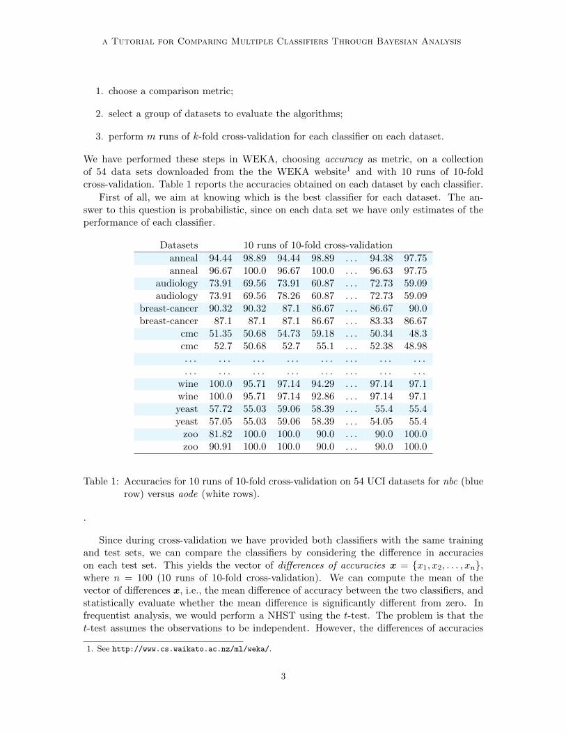
We have performed these steps in WEKA, choosing accuracy as metric, on a collectionof 54 data sets downloaded from the the WEKA website1 and with 10 runs of 10-foldcross-validation. Table 1 reports the accuracies obtained on each dataset by each classifier.
First of all, we aim at knowing which is the best classifier for each dataset. The an-swer to this question is probabilistic, since on each data set we have only estimates of theperformance of each classifier.
Datasets 10 runs of 10-fold cross-validation
anneal 94.44 98.89 94.44 98.89 . . . 94.38 97.75anneal 96.67 100.0 96.67 100.0 . . . 96.63 97.75
audiology 73.91 69.56 73.91 60.87 . . . 72.73 59.09audiology 73.91 69.56 78.26 60.87 . . . 72.73 59.09
breast-cancer 90.32 90.32 87.1 86.67 . . . 86.67 90.0breast-cancer 87.1 87.1 87.1 86.67 . . . 83.33 86.67
cmc 51.35 50.68 54.73 59.18 . . . 50.34 48.3cmc 52.7 50.68 52.7 55.1 . . . 52.38 48.98. . . . . . . . . . . . . . . . . . . . . . . .. . . . . . . . . . . . . . . . . . . . . . . .
wine 100.0 95.71 97.14 94.29 . . . 97.14 97.1wine 100.0 95.71 97.14 92.86 . . . 97.14 97.1yeast 57.72 55.03 59.06 58.39 . . . 55.4 55.4yeast 57.05 55.03 59.06 58.39 . . . 54.05 55.4
zoo 81.82 100.0 100.0 90.0 . . . 90.0 100.0zoo 90.91 100.0 100.0 90.0 . . . 90.0 100.0
Table 1: Accuracies for 10 runs of 10-fold cross-validation on 54 UCI datasets for nbc (bluerow) versus aode (white rows).
.
Since during cross-validation we have provided both classifiers with the same trainingand test sets, we can compare the classifiers by considering the difference in accuracieson each test set. This yields the vector of differences of accuracies x = {x1, x2, . . . , xn},where n = 100 (10 runs of 10-fold cross-validation). We can compute the mean of thevector of differences x, i.e., the mean difference of accuracy between the two classifiers, andstatistically evaluate whether the mean difference is significantly different from zero. Infrequentist analysis, we would perform a NHST using the t-test. The problem is that thet-test assumes the observations to be independent. However, the differences of accuracies
1. See http://www.cs.waikato.ac.nz/ml/weka/.
3
Alessio Benavoli, Giorgio Corani, Janez Demsar, Marco Zaffalon
are not independent of each other because of the overlapping training sets used in cross-validation. Thus the usual t-test is not calibrated when applied to the analysis of cross-validation results: when sampling the data under the null hypothesis its rate of Type I errorsis much larger than α (Dietterich, 1998). Moreover, the correlation cannot be estimatedfrom data; Nadeau and Bengio (2003) have proven that there is no unbiased estimator of thecorrelation of the results obtained on the different folds. Introducing some approximations,they have proposed a heuristic to choose the correlation parameter: ρ = nte
ntot, where nte,
ntr and ntot = nte + ntr respectively denote the size of the training set, of the test set andof the whole available data set.2
Frequentist correlated t-testThe correlated t-test is based on the modified Student’s t-statistic:
t(x, µ) =x− µ√
σ2( 1n + ρ
1−ρ)=
x− µ√σ2( 1
n + ntentr
), (1)
where x = 1n
∑ni=1 xi and σ =
√1
n−1
∑ni=1(xi − x)2 are the sample mean and sample
standard deviation of the data x, ρ is the correlation between the observations and µ is thevalue of the mean we aim at testing. The statistic follows a Student distribution with n− 1degrees of freedom:
St
(x;n− 1, µ,
(1
n+
ρ
1− ρ
)σ2
). (2)
For ρ = 0, we obtain the traditional t-test. For ρ = ntentot
, we obtain the correlated t-test proposed by Nadeau and Bengio (2003) to account for the correlation due to theoverlapping training sets. Usually the test is run in a two-sided fashion. Its hypotheses are:H0 : µ = 0; H1 : µ 6= 0. The p-value of the statistic under the null hypotheses is:
p = 2 · (1− Tn−1(|t(x, 0)|)), (3)
where Tn−1(|t(x, 0)|) denotes the cumulative distribution of the standardized Student distri-bution with n−1 degrees of freedom in |t(x, µ)| for µ = 0. For instance, for the first data setin Table 1 we have that x = −0.0194, σ = 0.01583, ρ = 1/10, n = 100 and so t(x, 0) = −3.52.Hence, the two-sided p-value is p = 2 · (1 − Tn−1(|t(x, 0)|)) = 0.00065 ≈ 0.001. Sometimesthe directional one-sided test is performed. If the alternative hypothesis is the positiveone, the hypotheses of the one-sided test are: H0 : µ ≤ 0; H1 : µ > 0. The p-value isp = 1− Tn−1(t(x, 0)).
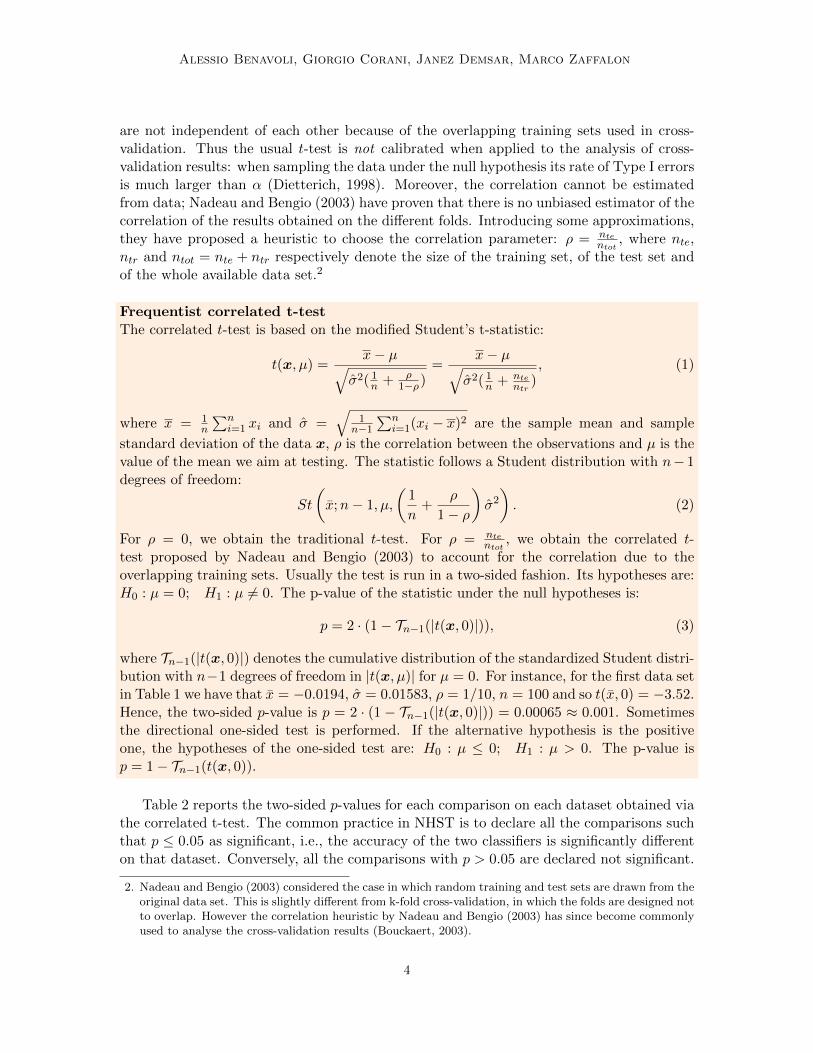
Table 2 reports the two-sided p-values for each comparison on each dataset obtained viathe correlated t-test. The common practice in NHST is to declare all the comparisons suchthat p ≤ 0.05 as significant, i.e., the accuracy of the two classifiers is significantly differenton that dataset. Conversely, all the comparisons with p > 0.05 are declared not significant.
2. Nadeau and Bengio (2003) considered the case in which random training and test sets are drawn from theoriginal data set. This is slightly different from k-fold cross-validation, in which the folds are designed notto overlap. However the correlation heuristic by Nadeau and Bengio (2003) has since become commonlyused to analyse the cross-validation results (Bouckaert, 2003).
4
a Tutorial for Comparing Multiple Classifiers Through Bayesian Analysis
Note that these significance tests can, under the NHST paradigm, only be considered inisolation, while combined they require either an omnibus test like ANOVA or correctionsfor multiple comparisons.
Dataset p-value Dataset p-value Dataset p-value
anneal 0.001 audiology 0.622 breast-cancer 0.598cmc 0.338 contact-lenses 0.643 credit 0.479
german-credit 0.171 pima-diabetes 0.781 ecoli 0.001eucalyptus 0.258 glass 0.162 grub-damage 0.090haberman 0.671 hayes-roth 1.000 cleeland-14 0.525
hungarian-14 0.878 hepatitis 0.048 hypothyroid 0.287ionosphere 0.684 iris 0.000 kr-s-kp 0.646
labor 1.000 lier-disorders 0.270 lymphography 0.018monks1 0.000 monks3 0.220 monks 0.000
mushroom 0.000 nursery 0.000 optdigits 0.000page 0.687 pasture 0.000 pendigits 0.452
postoperatie 0.582 primary-tumor 0.492 segment 0.000solar-flare-C 0.035 solar-flare-m 0.596 solar-flare-X 0.004
sonar 0.777 soybean 0.049 spambase 0.000spect-reordered 0.198 splice 0.004 squash-stored 0.940
squash-unstored 0.304 tae 0.684 credit 0.000owel 0.000 waveform 0.417 white-clover 0.463wine 0.671 yeast 0.576 zoo 0.435
Table 2: Two sided p-values for each dataset. The difference is significant (p < 0.05) in 19out of 54 comparisons.
2.1 NHST: the pitfalls of black and white thinking
Despite being criticized from its inception, NHST is still considered necessary for publica-tion, as p ≤ 0.05 is trusted as an objective proof of the method’s quality. One of the keyproblems of decisions based on p ≤ 0.05 is that it leads to “black and white thinking”,which ignores the fact that (i) a statistically significant difference is completely differentfrom a practically significant difference (Berger and Sellke, 1987); (ii) two methods thatare not statistically significantly different are not necessarily equivalent. The NHST andthis p-value-related “black and white thinking” do not allow for making informed decisions.Hereafter, we list the limits of NHST in order of severity using, as a working example, theassessment of the performance of classifiers.
NHST does not estimate probabilities of hypotheses. What is the probability thatthe performance of two classifiers is different (or equal)? This is the question we are askingwhen we compare two classifiers; and NHST cannot answer it.
In fact, the p-value represents the probability of getting the observed (or larger) differ-ences assuming that the performance of the classifiers is equal (H0). Formally, p = p(t(x) >
5
Alessio Benavoli, Giorgio Corani, Janez Demsar, Marco Zaffalon
τ |H0), where t(x) is the statistic computed from the data x, and τ is the critical value cor-responding to the test and the selected α. This is not the probability of the hypothesis,p(H0|x), in which we are interested.
Yet, researchers want to know the probability of the null and the alternative hypotheseson the basis of the observed data, rather than the probability of the data assuming thenull hypothesis to be true. Sentences like “at the 95% confidence level, we can concludethat (...)”, are formally correct, but they seem to imply that 1− p is the probability of thealternative hypothesis, while in fact 1− p = 1− p(t(x) > τ |H0) = p(t(x) < τ |H0), which isnot the same as p(H1|x). This is summed up in Table 3.
what we compute what we would like to know
p(t(x) > τ |H0) p(H0|x)1− p(t(x) > τ |H0) = p(t(x) < τ |H0) 1− p(H0|x) = p(H1|x)
Table 3: Difference between the probabilities of interest for the analyst and the probabilitiescomputed by the frequentist test.
Point-wise null hypotheses are practically always false. The difference betweentwo classifiers can be very small; however there are no two classifiers whose accuracies areperfectly equivalent.
By using a NHST, the null hypothesis is that the classifiers are equal. However, the nullhypothesis is practically always false! By rejecting the null hypothesis NHST indicates thatthe null hypothesis is unlikely; but this is known even before running the experiment. Thisproblem of the NHST has been pointed out in many different scientific domains (Lecoutreand Poitevineau, 2014, Sec 4.1.2.2). A consequence is that, since the null hypothesis isalways false, by adding enough data points it is possible to claim significanceeven when the effect size is trivial. This is because the p-value is affected both bythe sample size and the effect size, as discussed in the next section. Quoting Kruschke andLiddell (2015): “null hypotheses are straw men that can virtually always be rejected withenough data.”
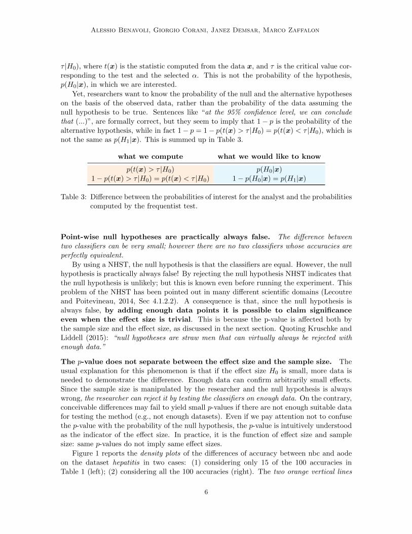
The p-value does not separate between the effect size and the sample size. Theusual explanation for this phenomenon is that if the effect size H0 is small, more data isneeded to demonstrate the difference. Enough data can confirm arbitrarily small effects.Since the sample size is manipulated by the researcher and the null hypothesis is alwayswrong, the researcher can reject it by testing the classifiers on enough data. On the contrary,conceivable differences may fail to yield small p-values if there are not enough suitable datafor testing the method (e.g., not enough datasets). Even if we pay attention not to confusethe p-value with the probability of the null hypothesis, the p-value is intuitively understoodas the indicator of the effect size. In practice, it is the function of effect size and samplesize: same p-values do not imply same effect sizes.
Figure 1 reports the density plots of the differences of accuracy between nbc and aodeon the dataset hepatitis in two cases: (1) considering only 15 of the 100 accuracies inTable 1 (left); (2) considering all the 100 accuracies (right). The two orange vertical lines
6
a Tutorial for Comparing Multiple Classifiers Through Bayesian Analysis
define the region in which the differences of accuracy is less than 1%—the meaning of theselines will be clarified in the next sections.
The p-value is 0.077 in the first case and so the null hypothesis cannot be rejected.The p-value becomes 0.048 in the second case and so the null hypothesis can be rejected.This demonstrates how adding data leads to rejection of the null hypothesis although thedifference between the two classifiers is very small in this dataset (all the mass is insidethe two orange vertical lines). Practical significance can be equated with the effect size,which is what the researcher is interested in. Statistical significance—the p-value—is not ameasure of practical significance, as shown in the example.
DeltaAcc
-0.02 -0.01 0.00 0.01 0.020
50
100
150
DeltaAcc
-0.02 -0.01 0.00 0.01 0.020
50
100
150
Figure 1: Density plot for the differences of accuracy between nbc and aode for the datasethepatitis considering only 15 of the 100 data (left) or all the data (right). Left: thenull hypothesis cannot be rejected (p = 0.077 > 0.05) using half the data. Right:the null hypothesis is rejected when all the data are considered (p = 0.048 < 0.05),despite the very small effect size.
NHST ignores magnitude and uncertainty. A very important problem with NHSTis that the result of the test does not provide information about the magnitude of the effector the uncertainty of its estimate, which are the key information we should aim at knowing.
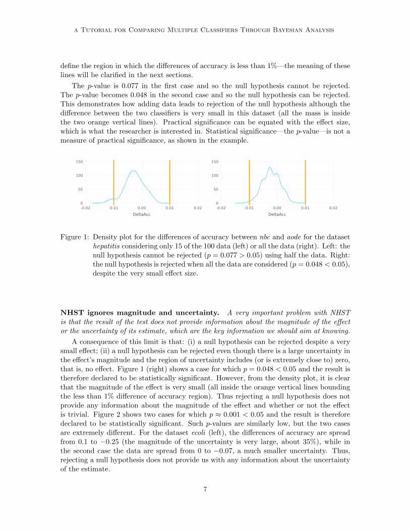
A consequence of this limit is that: (i) a null hypothesis can be rejected despite a verysmall effect; (ii) a null hypothesis can be rejected even though there is a large uncertainty inthe effect’s magnitude and the region of uncertainty includes (or is extremely close to) zero,that is, no effect. Figure 1 (right) shows a case for which p = 0.048 < 0.05 and the result istherefore declared to be statistically significant. However, from the density plot, it is clearthat the magnitude of the effect is very small (all inside the orange vertical lines boundingthe less than 1% difference of accuracy region). Thus rejecting a null hypothesis does notprovide any information about the magnitude of the effect and whether or not the effectis trivial. Figure 2 shows two cases for which p ≈ 0.001 < 0.05 and the result is thereforedeclared to be statistically significant. Such p-values are similarly low, but the two casesare extremely different. For the dataset ecoli (left), the differences of accuracy are spreadfrom 0.1 to −0.25 (the magnitude of the uncertainty is very large, about 35%), while inthe second case the data are spread from 0 to −0.07, a much smaller uncertainty. Thus,rejecting a null hypothesis does not provide us with any information about the uncertaintyof the estimate.
7
Alessio Benavoli, Giorgio Corani, Janez Demsar, Marco Zaffalon
DeltaAcc
-0.25 -0.20 -0.15 -0.10 -0.05 0.00 0.05 0.100
2
4
6
8
DeltaAcc
-0.25 -0.20 -0.15 -0.10 -0.05 0.00 0.05 0.100
10
20
30
Figure 2: Density plot for the differences of accuracy (DeltaAcc) between nbc and aode forthe datasets ecoli (left) and iris (right). The null hypothesis is rejected (p < 0.05)with similar p-values, even though the two cases have very different uncertainty.For ecoli, the uncertainty is very large and includes zero.
NHST yields no information about the null hypothesis. What can we say whenNHST does not reject the null hypothesis?
The scientific literature contains examples of non-significant tests interpreted as evidenceof no difference between the two methods/groups being compared. This is wrong sinceNHST cannot provide evidence in favour of the null hypothesis (see also Lecoutre andPoitevineau (2014, Sec 4.1.2.2) for further examples on this point). When NHST does notreject the null hypothesis, no conclusion can be made.
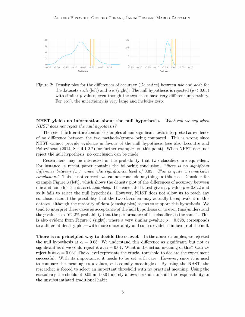
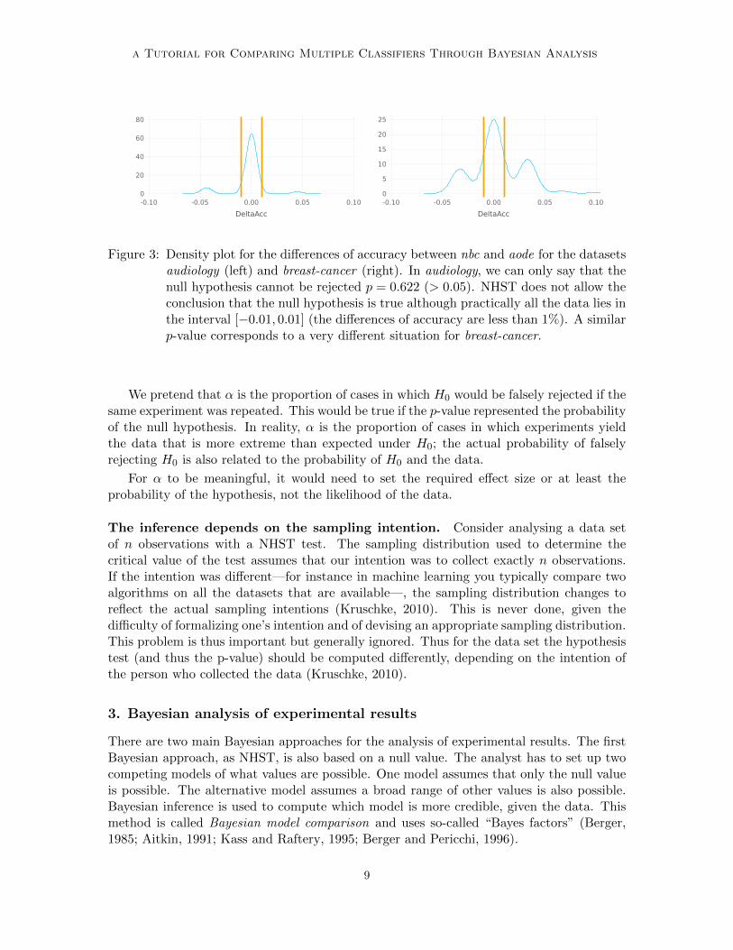
Researchers may be interested in the probability that two classifiers are equivalent.For instance, a recent paper contains the following conclusion: “there is no significantdifference between (...) under the significance level of 0.05. This is quite a remarkableconclusion.” This is not correct, we cannot conclude anything in this case! Consider forexample Figure 3 (left), which shows the density plot of the differences of accuracy betweennbc and aode for the dataset audiology. The correlated t-test gives a p-value p = 0.622 andso it fails to reject the null hypothesis. However, NHST does not allow us to reach anyconclusion about the possibility that the two classifiers may actually be equivalent in thisdataset, although the majority of data (density plot) seems to support this hypothesis. Wetend to interpret these cases as acceptance of the null hypothesis or to even (mis)understandthe p value as a “62.2% probability that the performance of the classifiers is the same”. Thisis also evident from Figure 3 (right), where a very similar p-value, p = 0.598, correspondsto a different density plot—with more uncertainty and so less evidence in favour of the null.
There is no principled way to decide the α level. In the above examples, we rejectedthe null hypothesis at α = 0.05. We understand this difference as significant, but not assignificant as if we could reject it at α = 0.01. What is the actual meaning of this? Can wereject it at α = 0.03? The α level represents the crucial threshold to declare the experimentsuccessful. With its importance, it needs to be set with care. However, since it is usedto compare the meaningless p-values, α is equally meaningless. By using the NHST, theresearcher is forced to select an important threshold with no practical meaning. Using thecustomary thresholds of 0.05 and 0.01 merely allows her/him to shift the responsibility tothe unsubstantiated traditional habit.
8
a Tutorial for Comparing Multiple Classifiers Through Bayesian Analysis
DeltaAcc
-0.10 -0.05 0.00 0.05 0.100
20
40
60
80
DeltaAcc
-0.10 -0.05 0.00 0.05 0.100
5
10
15
20
25
Figure 3: Density plot for the differences of accuracy between nbc and aode for the datasetsaudiology (left) and breast-cancer (right). In audiology, we can only say that thenull hypothesis cannot be rejected p = 0.622 (> 0.05). NHST does not allow theconclusion that the null hypothesis is true although practically all the data lies inthe interval [−0.01, 0.01] (the differences of accuracy are less than 1%). A similarp-value corresponds to a very different situation for breast-cancer.
We pretend that α is the proportion of cases in which H0 would be falsely rejected if thesame experiment was repeated. This would be true if the p-value represented the probabilityof the null hypothesis. In reality, α is the proportion of cases in which experiments yieldthe data that is more extreme than expected under H0; the actual probability of falselyrejecting H0 is also related to the probability of H0 and the data.
For α to be meaningful, it would need to set the required effect size or at least theprobability of the hypothesis, not the likelihood of the data.
The inference depends on the sampling intention. Consider analysing a data setof n observations with a NHST test. The sampling distribution used to determine thecritical value of the test assumes that our intention was to collect exactly n observations.If the intention was different—for instance in machine learning you typically compare twoalgorithms on all the datasets that are available—, the sampling distribution changes toreflect the actual sampling intentions (Kruschke, 2010). This is never done, given thedifficulty of formalizing one’s intention and of devising an appropriate sampling distribution.This problem is thus important but generally ignored. Thus for the data set the hypothesistest (and thus the p-value) should be computed differently, depending on the intention ofthe person who collected the data (Kruschke, 2010).
3. Bayesian analysis of experimental results
There are two main Bayesian approaches for the analysis of experimental results. The firstBayesian approach, as NHST, is also based on a null value. The analyst has to set up twocompeting models of what values are possible. One model assumes that only the null valueis possible. The alternative model assumes a broad range of other values is also possible.Bayesian inference is used to compute which model is more credible, given the data. Thismethod is called Bayesian model comparison and uses so-called “Bayes factors” (Berger,1985; Aitkin, 1991; Kass and Raftery, 1995; Berger and Pericchi, 1996).
9
Alessio Benavoli, Giorgio Corani, Janez Demsar, Marco Zaffalon
The second Bayesian approach does not set any null value. The analyst simply has toset up a range of candidate values (prior model), including the zero effect, and use Bayesianinference to compute the relative credibilities of all the candidate values (the posteriordistribution). This method is called Bayesian estimation (Gelman et al., 2014; Kruschke,2015).
The choice of the method depends on the situation – is a point-wise null hypothesisplausible ? (Bayarri and Berger, 2013, Sec.18.2.3.1)
In machine learning the estimation approach is preferable because there is not plausiblereason to believe that two different classifiers have exactly the same accuracy. For thisreason, we will focus on the Bayesian estimation approach that hereafter we will simply callBayesian analysis.
The first step in Bayesian analysis is establishing a descriptive mathematical model ofthe data. In a parametric model, this mathematical model is the the likelihood function thatprovides the probability of the observed data for each candidate value of the parameter(s)p(Data|θ). The second step is to establish the credibility for each value of the parameter(s)before observing data, the prior distribution p(θ). The third step is to use Bayes’ ruleto combine likelihood and prior to obtain the posterior distribution of the parameter(s)given the data p(θ|Data). The questions we pose in statistical analysis can be answered byquerying this posterior distribution in different ways.
As a concrete example of Bayesian analysis we will compare the accuracies of two com-peting classifiers via cross-validation on multiple data sets (Table 1). For this purpose, wewill adopt the correlated Bayesian t-test proposed by Corani and Benavoli (2015).
Bayesian correlated t-testThe Bayesian correlated t-test is used for the analysis of cross-validation results on a singledataset and it accounts for the correlation due to the overlapping training sets. The test isbased on the following (generative) model of the data:
xn×1 = 1n×1µ+ vn×1, (4)
where x = (x1, x2, . . . , xn) is the vector of differences of accuracy, 1n×1 is a vector of ones,µ is the parameter of interest (the mean difference of accuracy) and v ∼ MVN(0,Σn×n) isa multivariate Normal noise with zero mean and covariance matrix Σn×n. The covariancematrix Σ is characterized as follows: Σii = σ2 and Σij = σ2ρ for all i 6= j ∈ 1, . . . , n, whereρ is the correlation and σ2 is the variance and, therefore, the covariance matrix takes intoaccount the correlation due to cross-validation. Hence, the likelihood model of data is
p(x|µ,Σ) =exp(−1
2(x− 1µ)TΣ−1(x− 1µ))
(2π)n/2√|Σ|
. (5)
The likelihood (5) does not allow to estimate ρ from data, since the maximum likelihoodestimate of ρ is ρ = 0 regardless the observations (Corani and Benavoli, 2015). Thisconfirms that ρ is not identifiable: thus the Bayesian correlated t-test adopts the sameheuristic ρ = nte
ntotsuggested by Nadeau and Bengio (2003).
In Bayesian estimation, we aim at estimating the unknown parameters µ, ν = 1/σ2 andin particular µ, which is the parameter of interest in the Bayesian correlated t-test. To this
10
a Tutorial for Comparing Multiple Classifiers Through Bayesian Analysis
end, we consider the following prior:
p(µ, ν|µ0, k0, a, b) = N
(µ;µ0,
k0
ν
)G (ν; a, b) = NG(µ, ν;µ0, k0, a, b),
which is a Normal-Gamma distribution (Bernardo and Smith, 2009, Chap. 5) with parame-ters (µ0, k0, a, b). The Normal-Gamma prior is conjugate to the likelihood (5). If we choosethe prior parameters {µ0 = 0, k0 → ∞, a = −1/2, b = 0} (matching prior), the resultingposterior distribution of µ is the following Student distribution:
p(µ|x, µ0, k0, a, b) = St
(µ;n− 1, x,
(1
n+
ρ
1− ρ
)σ2
), (6)
where x =∑n
i=1 xin and σ2 =
∑ni=1(xi−x)2
n−1 . For these values of the prior parameters, theposterior distribution of µ (6) coincides with the Student distribution used in the fre-quentist correlated t-test in (2). For instance, consider the first data set in Table 1, wehave that x = −0.0194, σ = 0.01583, ρ = 1/10, n = 100 and so p(µ|x, µ0, k0, a, b) =St (µ; 99,−0.0194, 0.000030). The output of the Bayesian analysis is the posterior of µ,p(µ|x, µ0, k0, a, b), which we can plot and query.
In (6), we have reported the posterior distribution obtained under the matching prior—for which the probability of the Bayesian correlated t-test and the p-value of the frequentistcorrelated t-test are numerically equivalent. Our aim is to show that although they arenumerically equivalent the inferences drawn by the two approaches are very different. Inparticular we will show that a different interpretation of the same numerical value cancompletely change our prospective and allow us to make informative decisions. In otherwords, in this case the cassock does make the priest!
3.1 Comparing nbc and aode through Bayesian analysis: a colour thinking
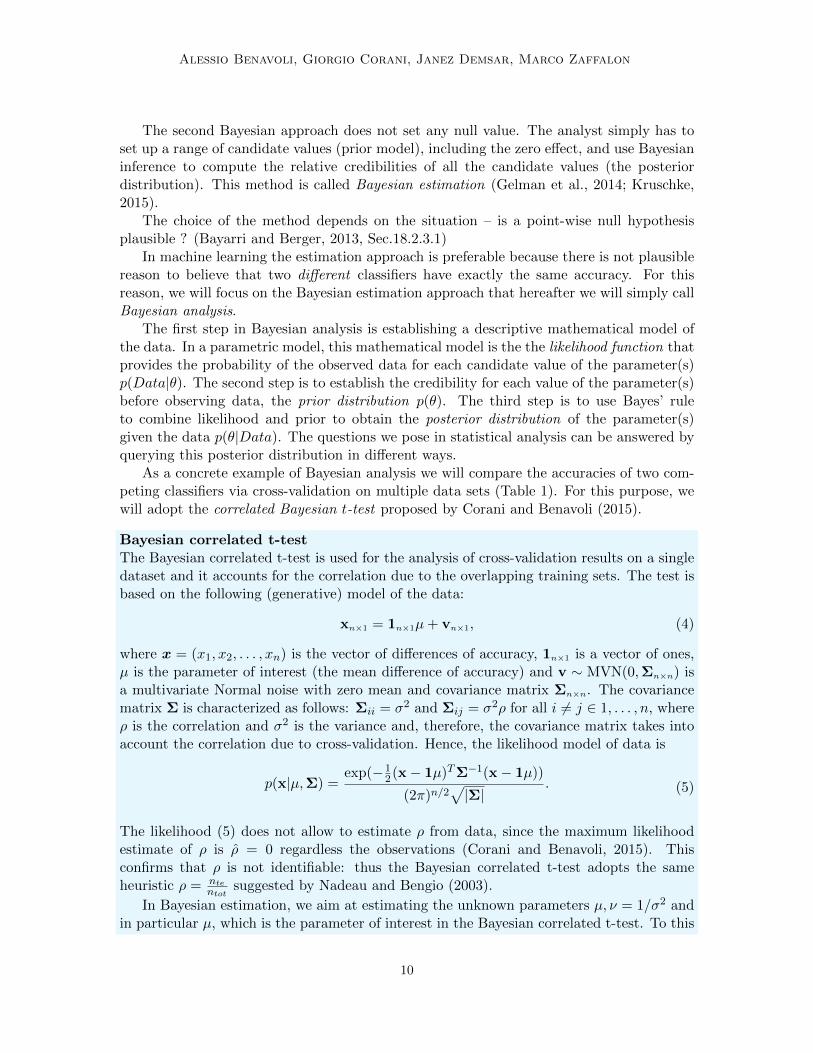
Consider the dataset squash-unsorted, with the posterior computed by the Bayesian corre-lated t-test for the difference between nbc and aode, as shown in Figure 4. The verticalorange lines mark again the region corresponding to a difference of accuracy of less than 1%(we will clarify the meaning of this region later in the section). In Bayesian analysis, theexperiment is summarized by the posterior distribution (in this case a Student distribution).The posterior describes the distribution of the mean difference of accuracies between thetwo classifiers.
By querying the posterior distribution, we can evaluate the probability of the hypothesis.We can for instance infer the probability that nbc is better/worse than aode. FormallyP (nbc > aode) = 0.165 is the integral of the posterior distribution from zero to infinity or,equivalently, the posterior probability that the mean of the differences of accuracy betweennbc and aode is greater than zero. P (aode > nbc) = 1 − P (nbc > aode) = 0.835 is theintegral of the posterior between minus infinity and zero or, equivalently, the posteriorprobability that the mean of the differences of accuracy is less than zero.
Can we say anything about the probability that nbc is practically equivalent to aode?Bayesian analysis can answer this question. First, we need to define the meaning of “prac-
11
Alessio Benavoli, Giorgio Corani, Janez Demsar, Marco Zaffalon
DeltaAcc
-0.2 -0.1 0.0 0.1 0.2
pdfrope
legend
0
2
4
6
8
Figure 4: Posterior of the Bayesian correlated t-test for the difference between nbc and aodein the dataset squash-unsorted.
tically equivalent”. In classification, it is sensible to define that two classifiers whose meandifference of accuracies is less that 1% are practically equivalent. The interval [−0.01, 0.01]thus defines a region of practical equivalence (rope) (Kruschke and Liddell, 2015) for clas-sifiers.3 Once we have defined a rope, from the posterior we can compute the probabilities:
• P (nbc � aode): the posterior probability of the mean difference of accuracies beingpractically negative, namely the integral of the posterior on the interval (−∞,−0.01).
• P (nbc = aode): the posterior probability of the two classifiers being practically equiv-alent, namely the integral of the posterior over the rope interval.
• P (nbc � aode): the posterior probability of the mean difference of accuracies beingpractically positive, namely the integral of the posterior on the interval (0.01,∞).
P (nbc = aode) = 0.086 is the integral of the posterior distribution between the vertical lines(the rope) shown in Figure 4 and it represents the probability that the two classifiers arepractically equivalent. Similarly, we can compute the probabilities that the two classifiersare practically different, which are P (nbc� aode) = 0.788 and P (nbc� aode) = 0.126.
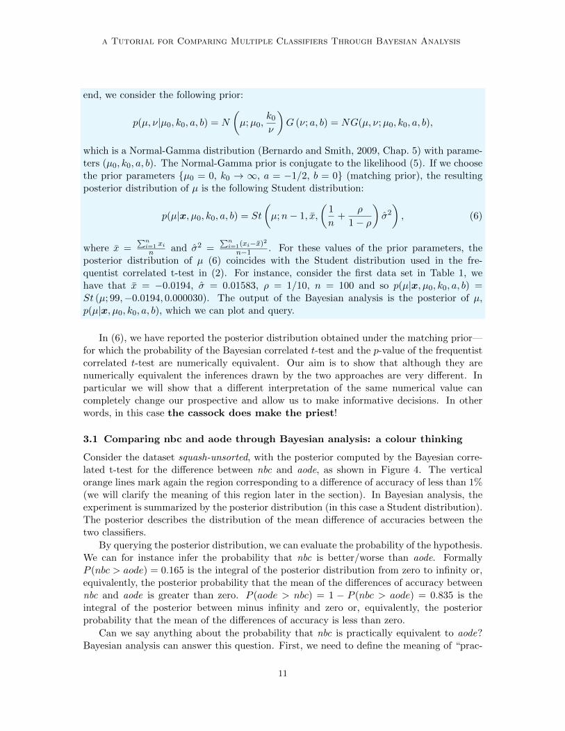
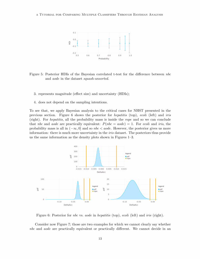
The posterior also shows the uncertainty in the estimate, because the distribution showsthe relative credibility of values across the continuum. One way to summarize the uncer-tainty is by marking the span of values that are the most credible and cover q% of thedistribution (e.g., q = 90%). These are called the High Density Intervals (HDIs) and theyare shown in Figure 5 (center) for q = 50, 60, 70, 80, 90, 95, 99.
Thus the posterior distribution equipped with rope:
1. estimates the posterior probability of a sensible null hypothesis (the area within therope);
2. claims significant differences that also have a practical meaning (the area outside therope);
3. In classification 1% seems to be a reasonable choice. However, in other domains a different value couldbe more suitable.
12
a Tutorial for Comparing Multiple Classifiers Through Bayesian Analysis
Probability
0.5 0.6 0.7 0.8 0.9 1.0-0.2
-0.1
0.0
0.1
HDI
Figure 5: Posterior HDIs of the Bayesian correlated t-test for the difference between nbcand aode in the dataset squash-unsorted.
3. represents magnitude (effect size) and uncertainty (HDIs);
4. does not depend on the sampling intentions.
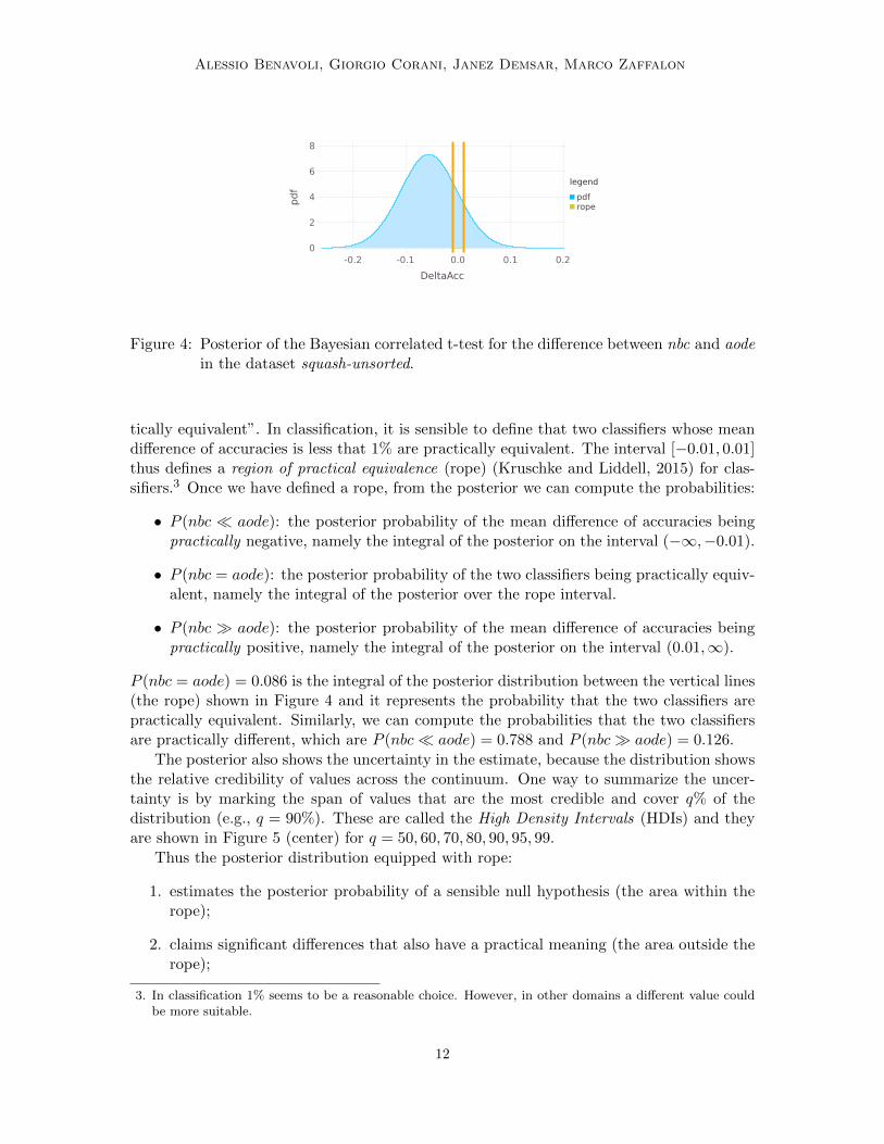
To see that, we apply Bayesian analysis to the critical cases for NHST presented in theprevious section. Figure 6 shows the posterior for hepatitis (top), ecoli (left) and iris(right). For hepatitis, all the probability mass is inside the rope and so we can concludethat nbc and aode are practically equivalent: P (nbc = aode) = 1. For ecoli and iris, theprobability mass is all in (−∞, 0] and so nbc < aode. However, the posterior gives us moreinformation: there is much more uncertainty in the iris dataset. The posteriors thus provideus the same information as the density plots shown in Figures 1–3.
DeltaAcc
-0.015 -0.010 -0.005 0.000 0.005 0.010 0.015
pdfrope
legend
0
100
200
300
400
DeltaAcc
-0.10 -0.05 0.00
pdfrope
legend
0
50
100
DeltaAcc
-0.10 -0.05 0.00
pdfrope
legend
0
5
10
15
20
Figure 6: Posterior for nbc vs. aode in hepatitis (top), ecoli (left) and iris (right).
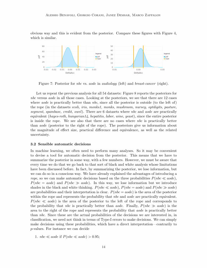
Consider now Figure 7; those are two examples for which we cannot clearly say whethernbc and aode are practically equivalent or practically different. We cannot decide in an
13
Alessio Benavoli, Giorgio Corani, Janez Demsar, Marco Zaffalon
obvious way and this is evident from the posterior. Compare these figures with Figure 4,which is similar.
DeltaAcc
-0.03 -0.02 -0.01 0.00 0.01 0.02 0.03
pdfrope
legend
0
20
40
60
80
DeltaAcc
-0.05 0.00 0.05
pdfrope
legend
0
10
20
30
40
50
Figure 7: Posterior for nbc vs. aode in audiology (left) and breast-cancer (right).
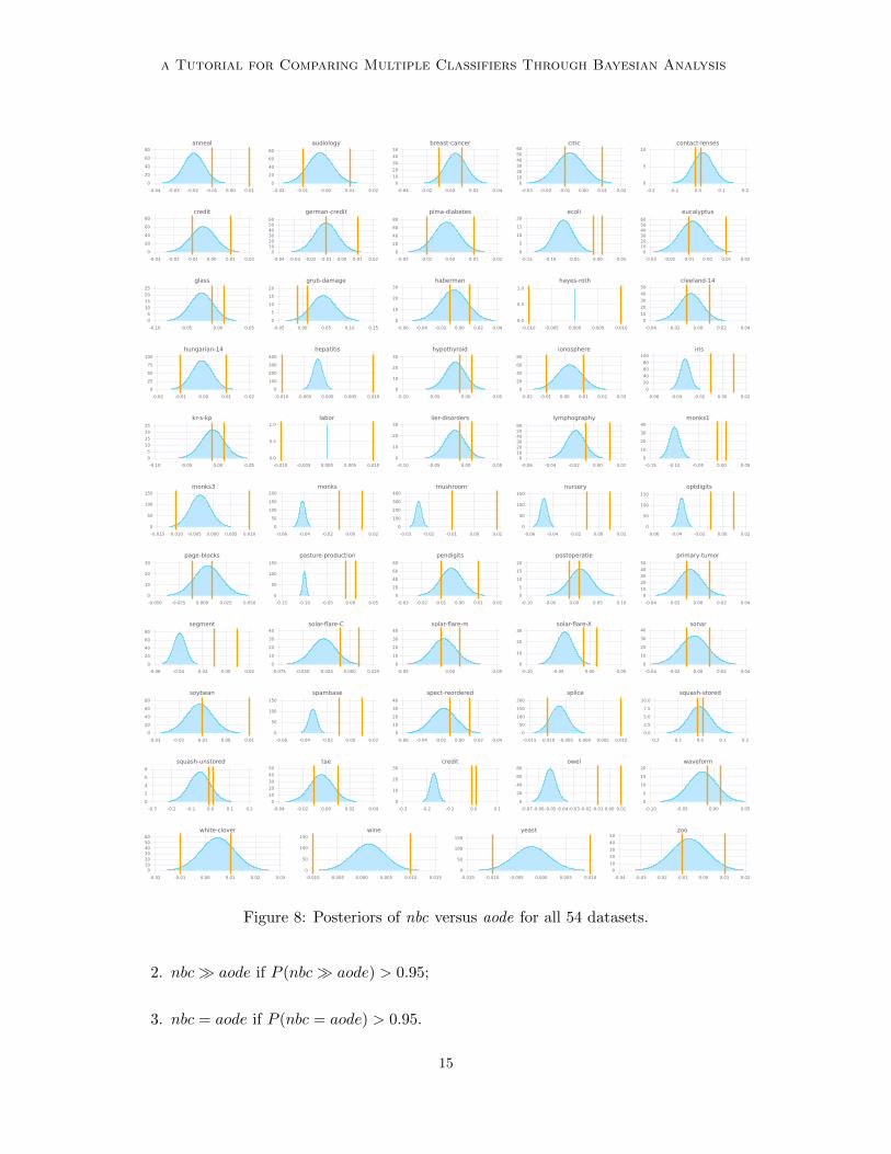
Let us repeat the previous analysis for all 54 datasets: Figure 8 reports the posteriors fornbc versus aode in all those cases. Looking at the posteriors, we see that there are 12 caseswhere aode is practically better than nbc, since all the posterior is outside (to the left of)the rope (in the datasets ecoli, iris, monks1, monks, mushroom, nursey, optdigits, pasture,segment, spambase, credit, owel). There are 6 datasets where nbc and aode are practicallyequivalent (hayes-roth, hungarian14, hepatitis, labor, wine, yeast), since the entire posterioris inside the rope. We see also that there are no cases where nbc is practically betterthan aode (posterior to the right of the rope). The posteriors give us information aboutthe magnitude of effect size, practical difference and equivalence, as well as the relateduncertainty.
3.2 Sensible automatic decisions
In machine learning, we often need to perform many analyses. So it may be convenientto devise a tool for automatic decision from the posterior. This means that we have tosummarize the posterior in some way, with a few numbers. However, we must be aware thatevery time we do that we go back to that sort of black and white analysis whose limitationshave been discussed before. In fact, by summarizing the posterior, we lose information, butwe can do so in a conscious way. We have already explained the advantages of introducing arope, so we can make automatic decisions based on the three probabilities P (nbc� aode),P (nbc = aode) and P (nbc � aode). In this way, we lose information but we introduceshades in the black and white thinking. P (nbc� aode), P (nbc = aode) and P (nbc� aode)are probabilities and their interpretation is clear. P (nbc = aode) is the area of the posteriorwithin the rope and represents the probability that nbc and aode are practically equivalent.P (nbc � aode) is the area of the posterior to the left of the rope and corresponds tothe probability that nbc is practically better than aode. Finally, P (nbc � aode) is thearea to the right of the rope and represents the probability that aode is practically betterthan nbc. Since these are the actual probabilities of the decisions we are interested in, inclassification, we need not think in terms of Type-I errors to make decisions. We can simplymake decisions using these probabilities, which have a direct interpretation—contrarily top-values. For instance we can decide
1. nbc� aode if P (nbc� aode) > 0.95;
14
a Tutorial for Comparing Multiple Classifiers Through Bayesian Analysis
-0.04 -0.03 -0.02 -0.01 0.00 0.01 0.02
0
10
20
30
40
50zoo
-0.015 -0.010 -0.005 0.000 0.005 0.010
0
50
100
150
yeast
-0.010 -0.005 0.000 0.005 0.010 0.015
0
50
100
150wine
-0.02 -0.01 0.00 0.01 0.02 0.03
0102030405060
white-clover
-0.10 -0.05 0.00 0.05
0
5
10
15
20waveform
-0.07 -0.06 -0.05 -0.04 -0.03 -0.02 -0.01 0.00 0.01
0
20
40
60
80owel
-0.3 -0.2 -0.1 0.0 0.1
0
10
20
30credit
-0.04 -0.02 0.00 0.02 0.04
0
10
20
30
40
50tae
-0.3 -0.2 -0.1 0.0 0.1 0.2
0
2
4
6
8
squash-unstored
-0.2 -0.1 0.0 0.1 0.2
0.0
2.5
5.0
7.5
10.0
squash-stored
-0.015 -0.010 -0.005 0.000 0.005 0.010
0
50
100
150
200
splice
-0.06 -0.04 -0.02 0.00 0.02 0.04
0
10
20
30
40
spect-reordered
-0.06 -0.04 -0.02 0.00 0.02
0
50
100
150
spambase
-0.03 -0.02 -0.01 0.00 0.01
0
20
40
60
80
soybean
-0.04 -0.02 0.00 0.02 0.04
0
10
20
30
40sonar
-0.10 -0.05 0.00 0.05
0
10
20
30solar-flare-X
-0.05 0.00 0.05
0
10
20
30
40solar-flare-m
-0.075 -0.050 -0.025 0.000 0.025
0
10
20
30
40solar-flare-C
-0.06 -0.04 -0.02 0.00 0.02
0
20
40
60
80
segment
-0.04 -0.02 0.00 0.02 0.04
0
10
20
30
40
50
primary-tumor
-0.10 -0.05 0.00 0.05 0.10
0
5
10
15
20
postoperatie
-0.03 -0.02 -0.01 0.00 0.01 0.02
0
20
40
60
80
pendigits
-0.15 -0.10 -0.05 0.00 0.05
0
50
100
150
pasture-production
-0.050 -0.025 0.000 0.025 0.050
0
10
20
30
page-blocks
-0.06 -0.04 -0.02 0.00 0.02
0
50
100
150
optdigits
-0.06 -0.04 -0.02 0.00 0.02
0
50
100
150
nursery
-0.03 -0.02 -0.01 0.00 0.01
0
100
200
300
400mushroom
-0.06 -0.04 -0.02 0.00 0.02
0
50
100
150
200monks
-0.015 -0.010 -0.005 0.000 0.005 0.010
0
50
100
150monks3
-0.15 -0.10 -0.05 0.00 0.05
0
10
20
30
40monks1
-0.06 -0.04 -0.02 0.00 0.02
0102030405060
lymphography
-0.10 -0.05 0.00 0.05
0
10
20
30lier-disorders
-0.010 -0.005 0.000 0.005 0.010
0.0
0.5
1.0labor
-0.10 -0.05 0.00 0.05
0
5
10
15
20
25
kr-s-kp
-0.06 -0.04 -0.02 0.00 0.02
0
20
40
60
80
100iris
-0.02 -0.01 0.00 0.01 0.02 0.03
0
20
40
60
80
ionosphere
-0.10 -0.05 0.00 0.05
0
10
20
30
hypothyroid
-0.010 -0.005 0.000 0.005 0.010
0
100
200
300
400
hepatitis
-0.02 -0.01 0.00 0.01 0.02
0
25
50
75
100
hungarian-14
-0.04 -0.02 0.00 0.02 0.04
0
10
20
30
40
50cleeland-14
-0.010 -0.005 0.000 0.005 0.010
0.0
0.5
1.0
hayes-roth
-0.06 -0.04 -0.02 0.00 0.02 0.04
0
10
20
30haberman
-0.05 0.00 0.05 0.10 0.15
0
5
10
15
20
grub-damage
-0.10 -0.05 0.00 0.05
0
5
10
15
20
25
glass
-0.03 -0.02 -0.01 0.00 0.01 0.02
0102030405060
eucalyptus
-0.15 -0.10 -0.05 0.00 0.05
0
5
10
15
20ecoli
-0.02 -0.01 0.00 0.01 0.02
0
20
40
60
80
pima-diabetes
-0.04 -0.03 -0.02 -0.01 0.00 0.01 0.02
0102030405060
german-credit
-0.03 -0.02 -0.01 0.00 0.01 0.02
0
20
40
60
80credit
-0.2 -0.1 0.0 0.1 0.2
0
5
10contact-lenses
-0.03 -0.02 -0.01 0.00 0.01 0.02
0102030405060
cmc
-0.04 -0.02 0.00 0.02 0.04
0
10
20
30
40
50breast-cancer
-0.02 -0.01 0.00 0.01 0.02
0
20
40
60
80
audiology
-0.04 -0.03 -0.02 -0.01 0.00 0.01
0
20
40
60
80anneal
Figure 8: Posteriors of nbc versus aode for all 54 datasets.
2. nbc� aode if P (nbc� aode) > 0.95;
3. nbc = aode if P (nbc = aode) > 0.95.
15
Alessio Benavoli, Giorgio Corani, Janez Demsar, Marco Zaffalon
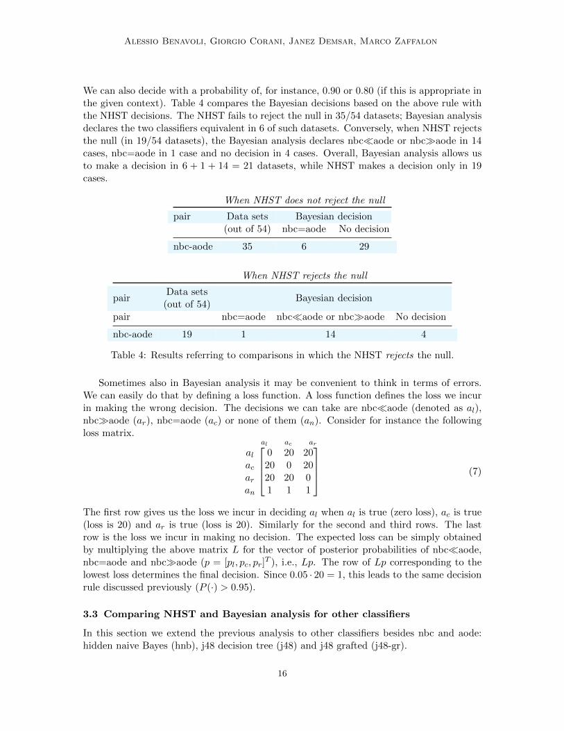
We can also decide with a probability of, for instance, 0.90 or 0.80 (if this is appropriate inthe given context). Table 4 compares the Bayesian decisions based on the above rule withthe NHST decisions. The NHST fails to reject the null in 35/54 datasets; Bayesian analysisdeclares the two classifiers equivalent in 6 of such datasets. Conversely, when NHST rejectsthe null (in 19/54 datasets), the Bayesian analysis declares nbc�aode or nbc�aode in 14cases, nbc=aode in 1 case and no decision in 4 cases. Overall, Bayesian analysis allows usto make a decision in 6 + 1 + 14 = 21 datasets, while NHST makes a decision only in 19cases.
When NHST does not reject the null
pair Data sets Bayesian decision(out of 54) nbc=aode No decision
nbc-aode 35 6 29
When NHST rejects the null
pairData sets
(out of 54)Bayesian decision
pair nbc=aode nbc�aode or nbc�aode No decision
nbc-aode 19 1 14 4
Table 4: Results referring to comparisons in which the NHST rejects the null.
Sometimes also in Bayesian analysis it may be convenient to think in terms of errors.We can easily do that by defining a loss function. A loss function defines the loss we incurin making the wrong decision. The decisions we can take are nbc�aode (denoted as al),nbc�aode (ar), nbc=aode (ac) or none of them (an). Consider for instance the followingloss matrix.
alacaran
al ac ar0 20 2020 0 2020 20 01 1 1
(7)
The first row gives us the loss we incur in deciding al when al is true (zero loss), ac is true(loss is 20) and ar is true (loss is 20). Similarly for the second and third rows. The lastrow is the loss we incur in making no decision. The expected loss can be simply obtainedby multiplying the above matrix L for the vector of posterior probabilities of nbc�aode,nbc=aode and nbc�aode (p = [pl, pc, pr]
T ), i.e., Lp. The row of Lp corresponding to thelowest loss determines the final decision. Since 0.05 · 20 = 1, this leads to the same decisionrule discussed previously (P (·) > 0.95).
3.3 Comparing NHST and Bayesian analysis for other classifiers
In this section we extend the previous analysis to other classifiers besides nbc and aode:hidden naive Bayes (hnb), j48 decision tree (j48) and j48 grafted (j48-gr).
16
a Tutorial for Comparing Multiple Classifiers Through Bayesian Analysis
The aim of this section is to show that the pattern described above is general and it alsoholds for other classifiers. The results are presented in two tables. First we report on thecases in which NHST does not reject the null (Tab. 5). Then we report on the comparisonsin which the NHST rejects the null (Tab. 6).
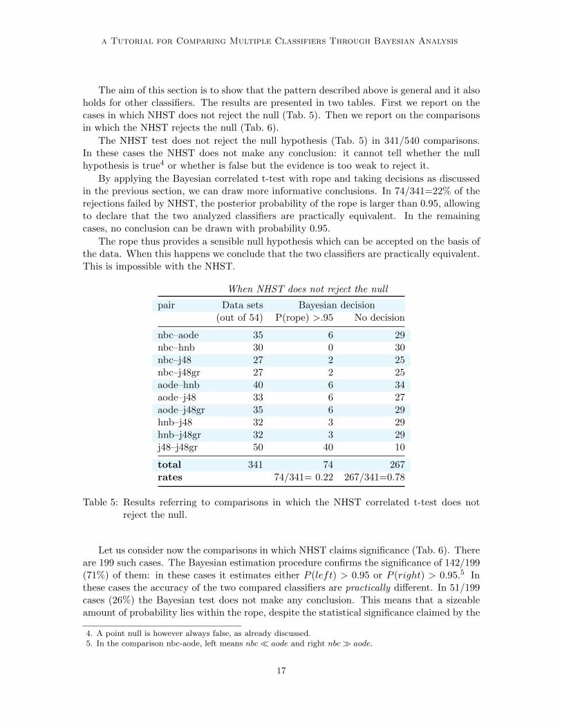
The NHST test does not reject the null hypothesis (Tab. 5) in 341/540 comparisons.In these cases the NHST does not make any conclusion: it cannot tell whether the nullhypothesis is true4 or whether is false but the evidence is too weak to reject it.
By applying the Bayesian correlated t-test with rope and taking decisions as discussedin the previous section, we can draw more informative conclusions. In 74/341=22% of therejections failed by NHST, the posterior probability of the rope is larger than 0.95, allowingto declare that the two analyzed classifiers are practically equivalent. In the remainingcases, no conclusion can be drawn with probability 0.95.
The rope thus provides a sensible null hypothesis which can be accepted on the basis ofthe data. When this happens we conclude that the two classifiers are practically equivalent.This is impossible with the NHST.
When NHST does not reject the null
pair Data sets Bayesian decision(out of 54) P(rope) >.95 No decision
nbc–aode 35 6 29nbc–hnb 30 0 30nbc–j48 27 2 25nbc–j48gr 27 2 25aode–hnb 40 6 34aode–j48 33 6 27aode–j48gr 35 6 29hnb–j48 32 3 29hnb–j48gr 32 3 29j48–j48gr 50 40 10
total 341 74 267rates 74/341= 0.22 267/341=0.78
Table 5: Results referring to comparisons in which the NHST correlated t-test does notreject the null.
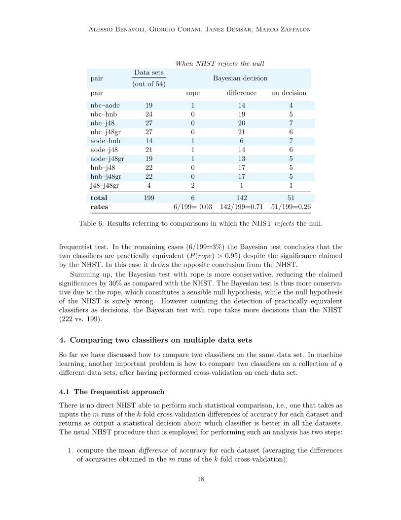
Let us consider now the comparisons in which NHST claims significance (Tab. 6). Thereare 199 such cases. The Bayesian estimation procedure confirms the significance of 142/199(71%) of them: in these cases it estimates either P (left) > 0.95 or P (right) > 0.95.5 Inthese cases the accuracy of the two compared classifiers are practically different. In 51/199cases (26%) the Bayesian test does not make any conclusion. This means that a sizeableamount of probability lies within the rope, despite the statistical significance claimed by the
4. A point null is however always false, as already discussed.5. In the comparison nbc-aode, left means nbc � aode and right nbc � aode.
17
Alessio Benavoli, Giorgio Corani, Janez Demsar, Marco Zaffalon
When NHST rejects the null
pairData sets
(out of 54)Bayesian decision
pair rope difference no decision
nbc–aode 19 1 14 4nbc–hnb 24 0 19 5nbc–j48 27 0 20 7nbc–j48gr 27 0 21 6aode–hnb 14 1 6 7aode–j48 21 1 14 6aode–j48gr 19 1 13 5hnb–j48 22 0 17 5hnb–j48gr 22 0 17 5j48–j48gr 4 2 1 1
total 199 6 142 51rates 6/199= 0.03 142/199=0.71 51/199=0.26
Table 6: Results referring to comparisons in which the NHST rejects the null.
frequentist test. In the remaining cases (6/199=3%) the Bayesian test concludes that thetwo classifiers are practically equivalent (P (rope) > 0.95) despite the significance claimedby the NHST. In this case it draws the opposite conclusion from the NHST.
Summing up, the Bayesian test with rope is more conservative, reducing the claimedsignificances by 30% as compared with the NHST. The Bayesian test is thus more conserva-tive due to the rope, which constitutes a sensible null hypothesis, while the null hypothesisof the NHST is surely wrong. However counting the detection of practically equivalentclassifiers as decisions, the Bayesian test with rope takes more decisions than the NHST(222 vs. 199).
4. Comparing two classifiers on multiple data sets
So far we have discussed how to compare two classifiers on the same data set. In machinelearning, another important problem is how to compare two classifiers on a collection of qdifferent data sets, after having performed cross-validation on each data set.
4.1 The frequentist approach
There is no direct NHST able to perform such statistical comparison, i.e., one that takes asinputs the m runs of the k-fold cross-validation differences of accuracy for each dataset andreturns as output a statistical decision about which classifier is better in all the datasets.The usual NHST procedure that is employed for performing such an analysis has two steps:
1. compute the mean difference of accuracy for each dataset (averaging the differencesof accuracies obtained in the m runs of the k-fold cross-validation);
18
a Tutorial for Comparing Multiple Classifiers Through Bayesian Analysis
2. perform a NHST to establish if the two classifiers have different performance or notbased on these mean differences of accuracy.
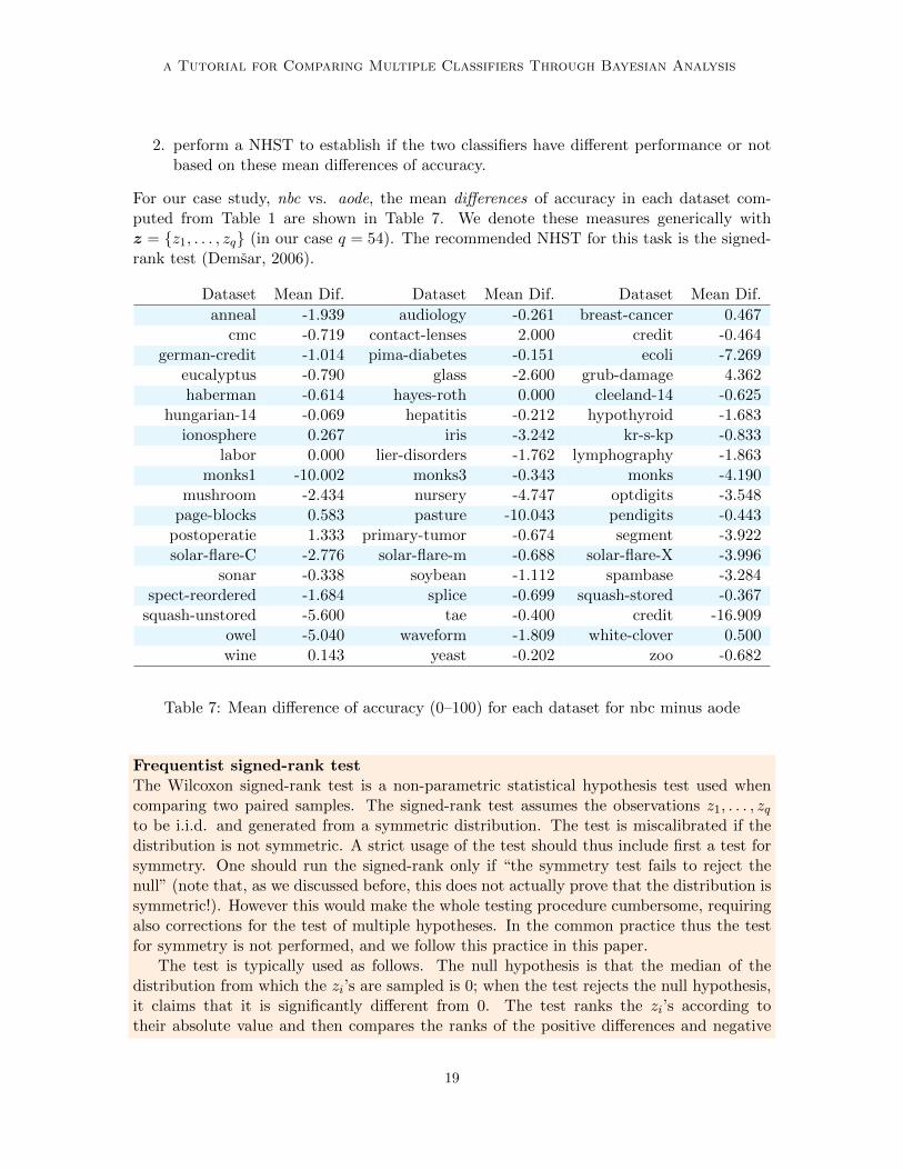
For our case study, nbc vs. aode, the mean differences of accuracy in each dataset com-puted from Table 1 are shown in Table 7. We denote these measures generically withz = {z1, . . . , zq} (in our case q = 54). The recommended NHST for this task is the signed-rank test (Demsar, 2006).
Dataset Mean Dif. Dataset Mean Dif. Dataset Mean Dif.
anneal -1.939 audiology -0.261 breast-cancer 0.467cmc -0.719 contact-lenses 2.000 credit -0.464
german-credit -1.014 pima-diabetes -0.151 ecoli -7.269eucalyptus -0.790 glass -2.600 grub-damage 4.362haberman -0.614 hayes-roth 0.000 cleeland-14 -0.625
hungarian-14 -0.069 hepatitis -0.212 hypothyroid -1.683ionosphere 0.267 iris -3.242 kr-s-kp -0.833
labor 0.000 lier-disorders -1.762 lymphography -1.863monks1 -10.002 monks3 -0.343 monks -4.190
mushroom -2.434 nursery -4.747 optdigits -3.548page-blocks 0.583 pasture -10.043 pendigits -0.443
postoperatie 1.333 primary-tumor -0.674 segment -3.922solar-flare-C -2.776 solar-flare-m -0.688 solar-flare-X -3.996
sonar -0.338 soybean -1.112 spambase -3.284spect-reordered -1.684 splice -0.699 squash-stored -0.367
squash-unstored -5.600 tae -0.400 credit -16.909owel -5.040 waveform -1.809 white-clover 0.500wine 0.143 yeast -0.202 zoo -0.682
Table 7: Mean difference of accuracy (0–100) for each dataset for nbc minus aode
Frequentist signed-rank testThe Wilcoxon signed-rank test is a non-parametric statistical hypothesis test used whencomparing two paired samples. The signed-rank test assumes the observations z1, . . . , zqto be i.i.d. and generated from a symmetric distribution. The test is miscalibrated if thedistribution is not symmetric. A strict usage of the test should thus include first a test forsymmetry. One should run the signed-rank only if “the symmetry test fails to reject thenull” (note that, as we discussed before, this does not actually prove that the distribution issymmetric!). However this would make the whole testing procedure cumbersome, requiringalso corrections for the test of multiple hypotheses. In the common practice thus the testfor symmetry is not performed, and we follow this practice in this paper.
The test is typically used as follows. The null hypothesis is that the median of thedistribution from which the zi’s are sampled is 0; when the test rejects the null hypothesis,it claims that it is significantly different from 0. The test ranks the zi’s according totheir absolute value and then compares the ranks of the positive differences and negative
19
Alessio Benavoli, Giorgio Corani, Janez Demsar, Marco Zaffalon
differences. The test statistic is:
t =∑
{i: zi≥0}ri(|zi|) =
∑1≤i≤j≤q
t+ij ,
where ri(|zi|) is the rank of |zi| and
t+ij =
{1 if zi ≥ −zj ,0 otherwise.
For instance, let us consider the following two cases z = {−2,−1, 4, 5} or z = {−1, 4, 5},then the statistic is t = 7 and, respectively, t = 5. For a large enough number of samples(e.g., q > 10), the statistic under the null hypothesis is approximately normally distributedand in this case the two-sided test is performed as follows:
w =t− q(q+1)
4√q(q+1)(2q+1)−tie
24
,
p = 2(1− Φ(|w|)),(8)
where p denotes the p-value computed w.r.t. Φ, which is the cumulative distribution functionof the standard Normal distribution; tie is an adjustment for ties in the data |z|, i.e.,zi = −zj for some i, j, required by the nonparametric test (Sidak et al., 1999; Hollanderet al., 2013), while it is zero in case of no ties.
Being non-parametric, the signed-rank is robust to outliers. It assumes commensura-bility of differences, but only qualitatively: greater differences count more as they top therank; yet their absolute magnitudes are ignored (Demsar, 2006).
4.1.1 Experimental results
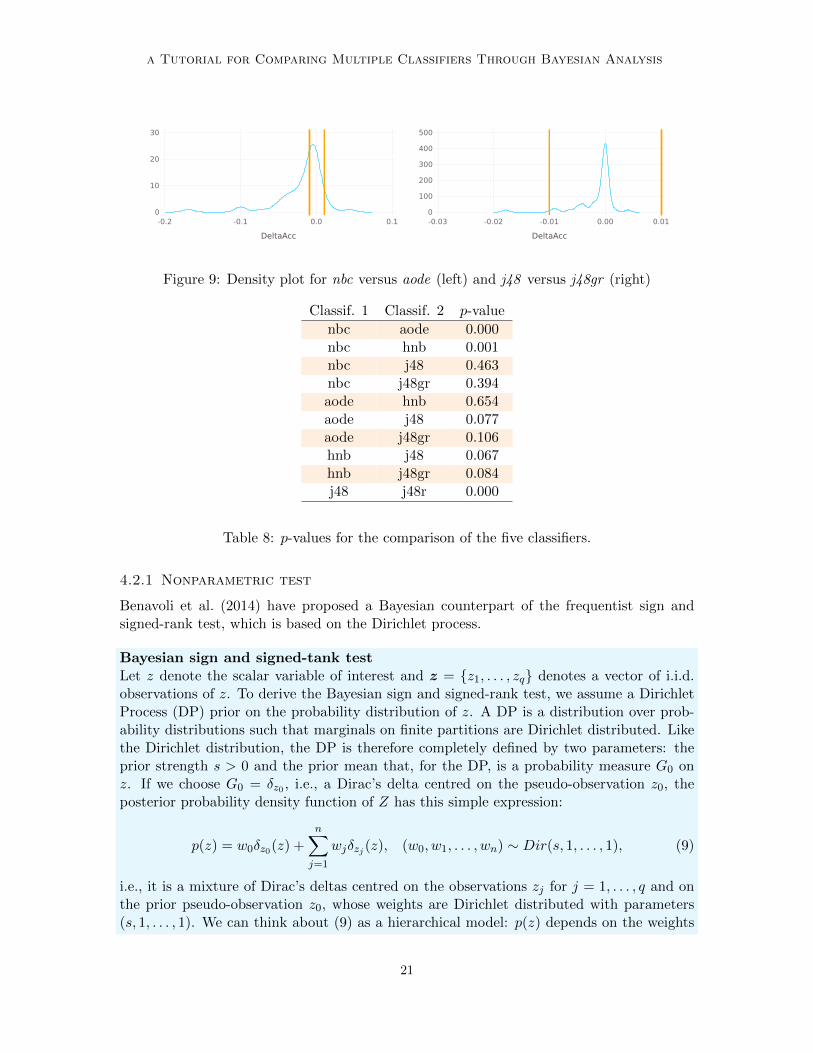
If we apply this method to compare nbc vs. aode, we obtain p-value=10−6 (the rank t = 162with no ties and w is −4.8). Since the p-value is less than 0.05, the NHST concludes thatthe null hypothesis can be rejected and that nbc and aode are significantly different. Table8 reports the p-values of all comparisons of the five classifiers. The pairs nbc-aode, nbc-hnb,j48-j48gr are statistically significantly different. Again by applying this black and whitemechanism, we encounter the same problems as before, i.e., we do not have any idea ofthe magnitude of the effect size, the uncertainty, the probability of the null hypothesis, etcetera. The density plot of the data (the mean differences of accuracy in each dataset) fornbc versus aode shows for instance that there are many datasets where the mean differenceis small (close to zero), see Figure 9. Instead for j48 versus j48gr, it is clear that thedifference of accuracy is very small.
4.2 The Bayesian analysis approach
We will present two ways of approaching the comparison between two classifiers in multipledatasets. The first will be based on a nonparametric approach that directly extends theWilcoxon signed-rank test. The second is a hierarchical model.
20
a Tutorial for Comparing Multiple Classifiers Through Bayesian Analysis
DeltaAcc
-0.2 -0.1 0.0 0.10
10
20
30
DeltaAcc
-0.03 -0.02 -0.01 0.00 0.010
100
200
300
400
500
Figure 9: Density plot for nbc versus aode (left) and j48 versus j48gr (right)
Classif. 1 Classif. 2 p-value
nbc aode 0.000nbc hnb 0.001nbc j48 0.463nbc j48gr 0.394aode hnb 0.654aode j48 0.077aode j48gr 0.106hnb j48 0.067hnb j48gr 0.084j48 j48r 0.000
Table 8: p-values for the comparison of the five classifiers.
4.2.1 Nonparametric test
Benavoli et al. (2014) have proposed a Bayesian counterpart of the frequentist sign andsigned-rank test, which is based on the Dirichlet process.
Bayesian sign and signed-tank testLet z denote the scalar variable of interest and z = {z1, . . . , zq} denotes a vector of i.i.d.observations of z. To derive the Bayesian sign and signed-rank test, we assume a DirichletProcess (DP) prior on the probability distribution of z. A DP is a distribution over prob-ability distributions such that marginals on finite partitions are Dirichlet distributed. Likethe Dirichlet distribution, the DP is therefore completely defined by two parameters: theprior strength s > 0 and the prior mean that, for the DP, is a probability measure G0 onz. If we choose G0 = δz0 , i.e., a Dirac’s delta centred on the pseudo-observation z0, theposterior probability density function of Z has this simple expression:
p(z) = w0δz0(z) +
n∑j=1
wjδzj (z), (w0, w1, . . . , wn) ∼ Dir(s, 1, . . . , 1), (9)
i.e., it is a mixture of Dirac’s deltas centred on the observations zj for j = 1, . . . , q and onthe prior pseudo-observation z0, whose weights are Dirichlet distributed with parameters(s, 1, . . . , 1). We can think about (9) as a hierarchical model: p(z) depends on the weights
21
Alessio Benavoli, Giorgio Corani, Janez Demsar, Marco Zaffalon
w that are Dirichlet distributed. The model (9) is therefore a posterior distribution of theprobability distribution of z and encloses all the information we need for the experimentalanalysis. We can summarize it in different way. If we compute:
θl = P (z < −r) =
q∑i=0
wiI(−∞,−r)(zi),
θe = P (|z| ≤ r) =
q∑i=0
wiI[−r,r](zi),
θr = P (z > r) =
q∑i=0
wiI(r,∞)(zi),
where the indicator IA(z) = 1 if z0 ∈ A and zero otherwise, then we obtain a Bayesianversion of the sign test that also accounts for the rope [−r, r]. In fact, θl, θe, θr are respec-tively the probabilities that the mean difference of accuracy is in the interval (−∞,−r),[−r, r], or (r,∞). Since (w0, w1, . . . , wn) ∼ Dir(s, 1, . . . , 1), it can easily be shown that
θl, θe, θr ∼ Dirichlet(nl + sI(−∞,−r](z0), ne + sI[−r,r](z0), nr + sI[r,∞)(z0)), (10)
where nl is the number of observations zi that fall in (−∞,−r], ne is the number of observa-tions zi that fall in [−r, r] and nr is the number of observations zi that fall in [r,∞), obviouslynl +ne +nr = q. If we neglect sI(−∞,−r](z0), sI[−r,r](z0), sI[r,∞)(z0), then (10) says that theposterior probability of θl, θe, θr is Dirichlet distributed with parameters (nl, ne, nr). Theterms sI(−∞,−r](z0), sI[−r,r](z0), sI[r,∞)(z0) are due to the prior. Therefore, to fully specifythe Bayesian sign test, we must choose the value of the prior strength s and where to placethe pseudo-observation z0 in (−∞,−r] or [−r, r] or [r,∞). We will return to this choice inSection 4.3. Instead, if we compute
θl =
q∑i=0
q∑j=0
wiwjI(−∞,−2r)(zj + zi),
θe =
q∑i=0
q∑j=0
wiwjI[−2r,2r](zj + zi),
θr =
q∑i=0
q∑j=0
wiwjI(2r,∞)(zj + zi), (11)
then we derive a Bayesian version of the signed rank test (Benavoli et al., 2014) that alsoaccounts for the rope [−r, r]. This time the distribution of θl, θe, θr has not a simple closedform but we can easily compute it by Monte Carlo sampling the weights (w0, w1, . . . , wn) ∼Dir(s, 1, . . . , 1). Also in this case we must choose s, z0, see Section 4.3.
It should be observed that the Bayesian signed-rank test does not require the symmetryassumption about the distribution of the observations zi. This test works also in case thedistribution is asymmetric thanks to the Bayesian estimation approach (i.e., it estimates
22
a Tutorial for Comparing Multiple Classifiers Through Bayesian Analysis
the distribution from data). This is another advantage of the Bayesian estimation approachw.r.t. the frequentist null hypothesis tests (Benavoli et al., 2014).
4.2.2 Experiments
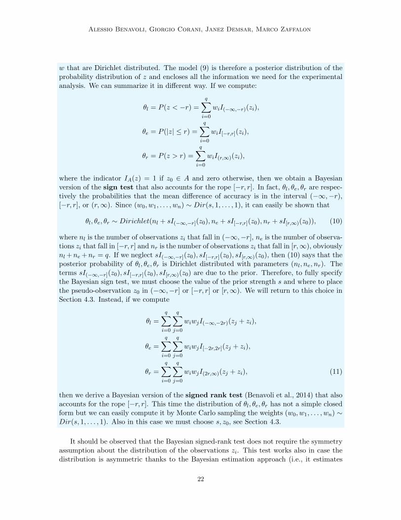
Let us start by comparing nbc vs. aode by means of the Bayesian sign-rank tests withoutrope (r = 0). Hereafter we will choose the prior parameter of the Dirichlet as s = 0.5 andz0 = 0; we will return to this choice in Section 4.3. Since without rope θr = 1 − θl, wehave only reported the posterior of θl (denoted as “Pleft”) that represents the probabilitythat aode is better than nbc. The samples of the posteriors are shown in Figure 10: this issimply the histogram of 150′000 samples of θl generated according to (11). For all samples,it results in θl greater than 0.5 and so θr = 1− θl. So we can conclude with probability ≈ 1that aode is better than nbc. We can in fact think about the comparison of two classifiersas the inference on the bias (θl) of a coin. In this case, all the 150′000 sampled coins fromthe posterior have a bias that is greater than 0.5 and, therefore, all the coins are alwaysbiased towards aode (which is then preferable to nbc).
This conclusion is in agreement with that derived by the frequentist sign-rank test (verysmall p-value, see Table 8).
Pleft
0.5 0.6 0.7 0.8 0.9 1.00
500
1000
1500
Figure 10: Posterior for nbc vs. aode for the Bayesian sign-rank test.
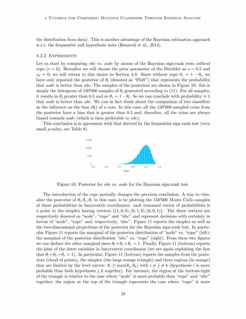
The introduction of the rope partially changes the previous conclusion. A way to visu-alize the posterior of θl, θe, θr in this case, is by plotting the 150′000 Monte Carlo samplesof these probabilities in barycentric coordinates: each trinomial vector of probabilities isa point in the simplex having vertices {(1, 0, 0), (0, 1, 0), (0, 0, 1)}. The three vertices arerespectively denoted as “aode”, “rope” and “nbc” and represent decisions with certainty infavour of “aode”, “rope” and, respectively, “nbc”. Figure 11 reports the simplex as well asthe two-dimensional projections of the posterior for the Bayesian sign-rank test. In partic-ular Figure 11 reports the marginal of the posterior distribution of “aode” vs. “rope” (left);the marginal of the posterior distribution “nbc” vs. “rope” (right). From these two figureswe can deduce the other marginal since θl+θe+θr = 1. Finally, Figure 11 (bottom) reportsthe joint of the three variables in barycentric coordinates (we are again exploiting the factthat θl+θe+θr = 1). In particular, Figure 11 (bottom) reports the samples from the poste-riors (cloud of points), the simplex (the large orange triangle) and three regions (in orange)that are limited by the level curves: θi ≥ max(θj , θk) with i 6= j 6= k (hypothesis i is moreprobable than both hypotheses j, k together). For instance, the region at the bottom-rightof the triangle is relative to the case where “aode” is more probable than “rope” and “nbc”together; the region at the top of the triangle represents the case where “rope” is more
23
Alessio Benavoli, Giorgio Corani, Janez Demsar, Marco Zaffalon
aode
0.0 0.5 1.01
200
50
100
150
Count
0.0
0.2
0.4
0.6
0.8
rope
nbc
0.0 0.1 0.2 0.3
1
100
50
Count
0.0
0.2
0.4
0.6
0.8
rope
1
25
50
75
100
Count
rope
aodenbc
Figure 11: Posterior for nbc vs. aode for the Bayesian sign-rank test.
probable than “aode” and “nbc” together; the region at the left of the triangle correspondsto the case where “nbc” is more probable than “aode” and “rope” together. Hence, if allthe points fall inside one of these three regions, we conclude that such hypothesis is truewith probability ≈ 1. Looking at Figure 11 (bottom), it is evident that the majority ofcases support aode more than rope and definitively more than nbc. We can quantify thisnumerically by counting the number of points that fall in the three regions, see first rowin Table 9. aode is better in 90% of cases, while rope is selected in the remaining 10%.We can therefore conclude with probability 90% that aode is practically better than nbc.Table 9 reports also these probabilities for the other comparisons of classifiers computedusing 150′000 Monte Carlo samples. We conclude that hnb is practically better than nbcwith probability 0.999; aode and hnb are equivalent with probability 0.95; aode is betterthan j48 and j48gr with probability 0.9; hnb is better than j48 and j48gr with probabilitygreater than 0.95 and finally j48 and j48gr are practically equivalent. These conclusionsare in agreement with the data.
The computational complexity of the Bayesian sign-rank test is low. The comparisonof two classifiers (based on 150′000 samples) takes less than one second on a standardcomputer.
4.3 Choice of the prior
In the previous section, we have selected the prior parameters of the Dirichlet process ass = 0.5 and z0 = 0. In terms of rank, this basically means that the prior strength is
24
a Tutorial for Comparing Multiple Classifiers Through Bayesian Analysis
500
1500
1000
1
Count
rope
j48grj48
10
50
30
1
20
40
Count
rope
j48grhnb
30
20
10
60
40
1
50
Count
rope
j48hnb
10
50
30
1
20
40
Count
rope
j48graode
10
50
30
1
20
40
Count
rope
j48aode
10
50
30
1
20
40
Count
rope
hnbaode
30
20
10
60
40
1
50
Count
rope
j48grnbc
30
20
10
60
40
1
50
Count
rope
j48nbc
30
20
10
60
40
1
50
Count
rope
hnbnbc
Figure 12: Posterior for nbc vs. aode for Bayesian sign-rank test.
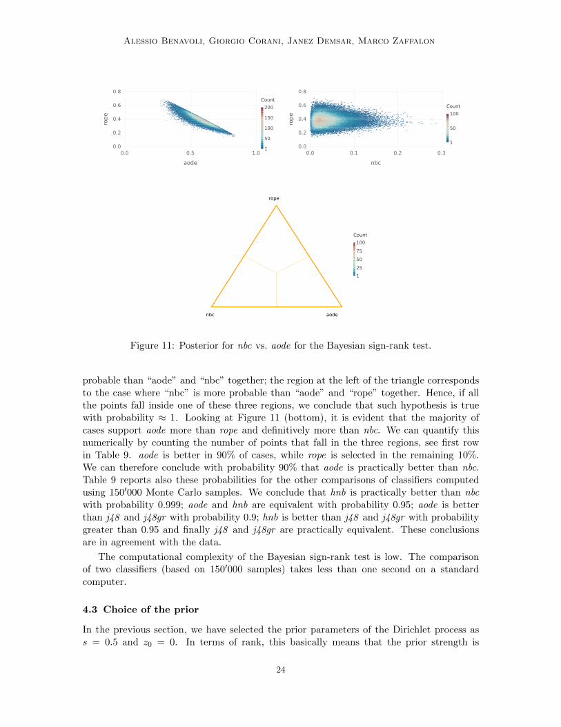
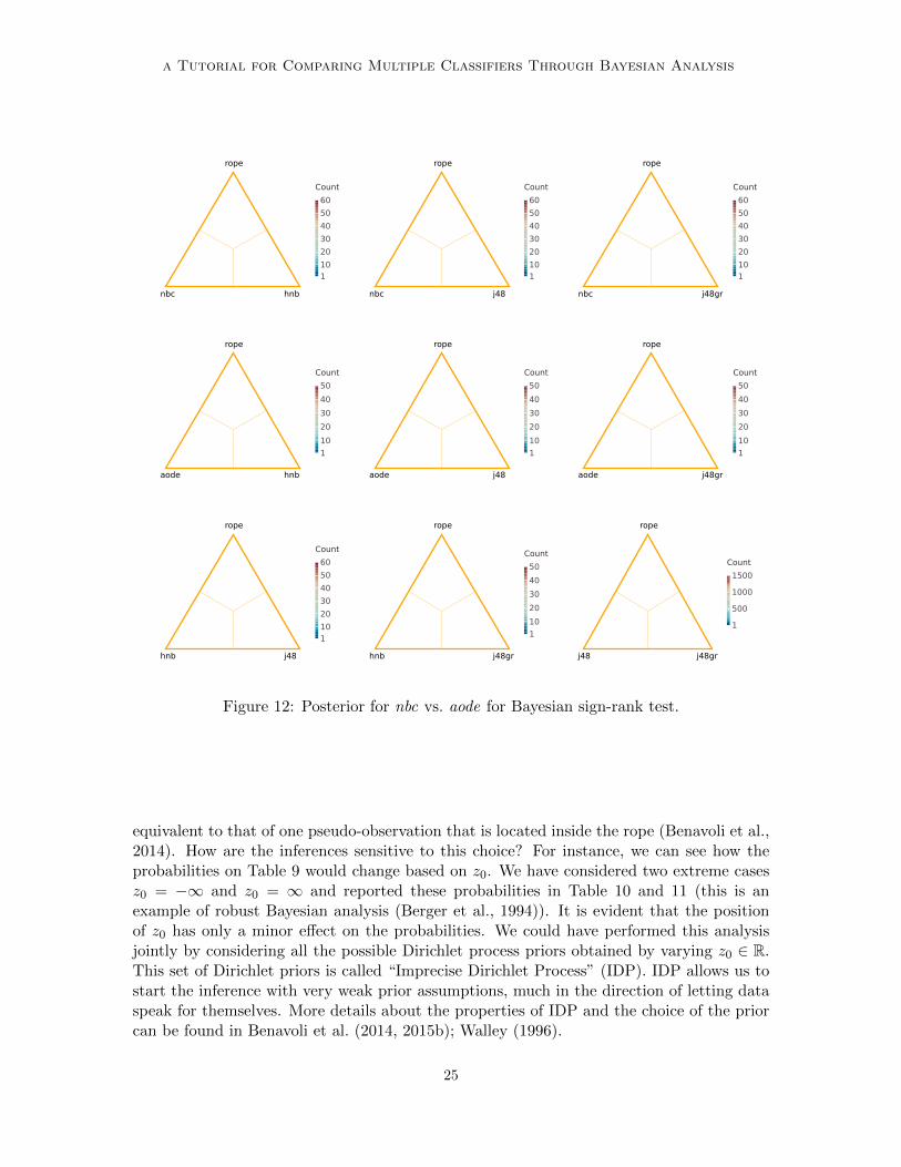
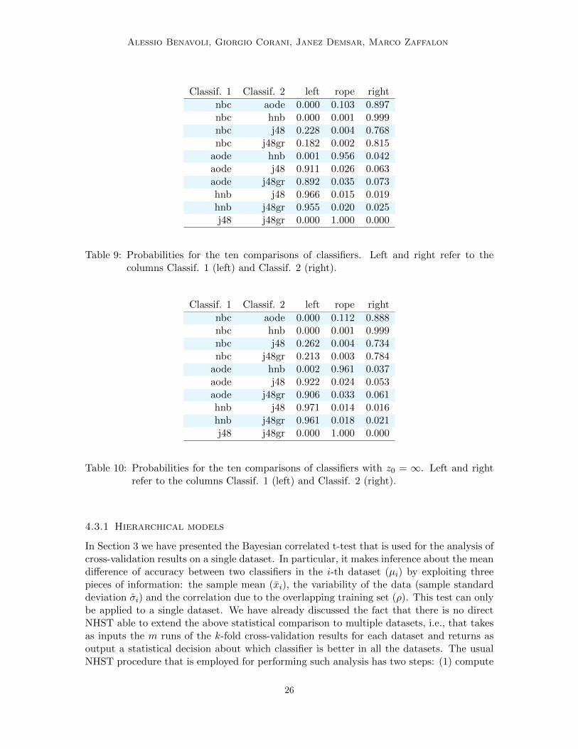
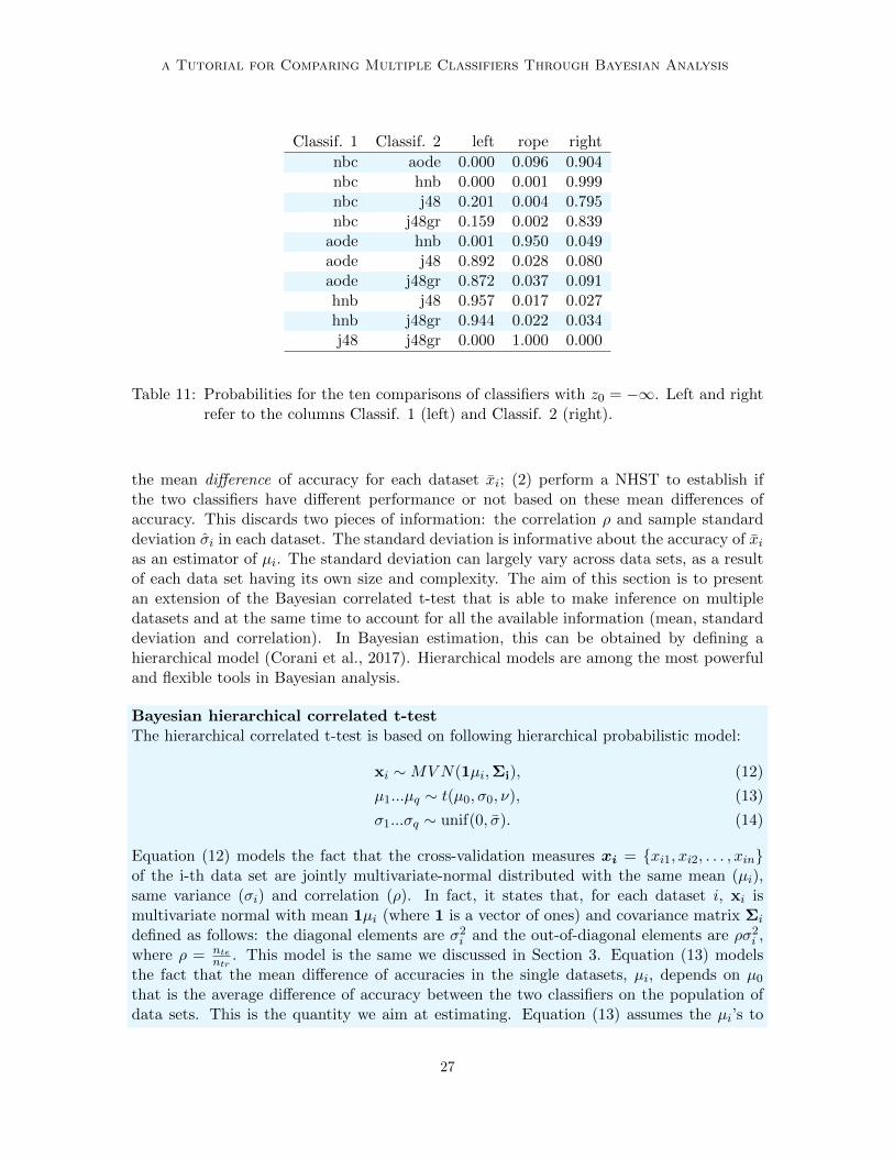
equivalent to that of one pseudo-observation that is located inside the rope (Benavoli et al.,2014). How are the inferences sensitive to this choice? For instance, we can see how theprobabilities on Table 9 would change based on z0. We have considered two extreme casesz0 = −∞ and z0 = ∞ and reported these probabilities in Table 10 and 11 (this is anexample of robust Bayesian analysis (Berger et al., 1994)). It is evident that the positionof z0 has only a minor effect on the probabilities. We could have performed this analysisjointly by considering all the possible Dirichlet process priors obtained by varying z0 ∈ R.This set of Dirichlet priors is called “Imprecise Dirichlet Process” (IDP). IDP allows us tostart the inference with very weak prior assumptions, much in the direction of letting dataspeak for themselves. More details about the properties of IDP and the choice of the priorcan be found in Benavoli et al. (2014, 2015b); Walley (1996).
25
Alessio Benavoli, Giorgio Corani, Janez Demsar, Marco Zaffalon
Classif. 1 Classif. 2 left rope right
nbc aode 0.000 0.103 0.897nbc hnb 0.000 0.001 0.999nbc j48 0.228 0.004 0.768nbc j48gr 0.182 0.002 0.815
aode hnb 0.001 0.956 0.042aode j48 0.911 0.026 0.063aode j48gr 0.892 0.035 0.073hnb j48 0.966 0.015 0.019hnb j48gr 0.955 0.020 0.025j48 j48gr 0.000 1.000 0.000
Table 9: Probabilities for the ten comparisons of classifiers. Left and right refer to thecolumns Classif. 1 (left) and Classif. 2 (right).
Classif. 1 Classif. 2 left rope right
nbc aode 0.000 0.112 0.888nbc hnb 0.000 0.001 0.999nbc j48 0.262 0.004 0.734nbc j48gr 0.213 0.003 0.784
aode hnb 0.002 0.961 0.037aode j48 0.922 0.024 0.053aode j48gr 0.906 0.033 0.061hnb j48 0.971 0.014 0.016hnb j48gr 0.961 0.018 0.021j48 j48gr 0.000 1.000 0.000
Table 10: Probabilities for the ten comparisons of classifiers with z0 = ∞. Left and rightrefer to the columns Classif. 1 (left) and Classif. 2 (right).
4.3.1 Hierarchical models
In Section 3 we have presented the Bayesian correlated t-test that is used for the analysis ofcross-validation results on a single dataset. In particular, it makes inference about the meandifference of accuracy between two classifiers in the i-th dataset (µi) by exploiting threepieces of information: the sample mean (xi), the variability of the data (sample standarddeviation σi) and the correlation due to the overlapping training set (ρ). This test can onlybe applied to a single dataset. We have already discussed the fact that there is no directNHST able to extend the above statistical comparison to multiple datasets, i.e., that takesas inputs the m runs of the k-fold cross-validation results for each dataset and returns asoutput a statistical decision about which classifier is better in all the datasets. The usualNHST procedure that is employed for performing such analysis has two steps: (1) compute
26
a Tutorial for Comparing Multiple Classifiers Through Bayesian Analysis
Classif. 1 Classif. 2 left rope right
nbc aode 0.000 0.096 0.904nbc hnb 0.000 0.001 0.999nbc j48 0.201 0.004 0.795nbc j48gr 0.159 0.002 0.839
aode hnb 0.001 0.950 0.049aode j48 0.892 0.028 0.080aode j48gr 0.872 0.037 0.091hnb j48 0.957 0.017 0.027hnb j48gr 0.944 0.022 0.034j48 j48gr 0.000 1.000 0.000
Table 11: Probabilities for the ten comparisons of classifiers with z0 = −∞. Left and rightrefer to the columns Classif. 1 (left) and Classif. 2 (right).
the mean difference of accuracy for each dataset xi; (2) perform a NHST to establish ifthe two classifiers have different performance or not based on these mean differences ofaccuracy. This discards two pieces of information: the correlation ρ and sample standarddeviation σi in each dataset. The standard deviation is informative about the accuracy of xias an estimator of µi. The standard deviation can largely vary across data sets, as a resultof each data set having its own size and complexity. The aim of this section is to presentan extension of the Bayesian correlated t-test that is able to make inference on multipledatasets and at the same time to account for all the available information (mean, standarddeviation and correlation). In Bayesian estimation, this can be obtained by defining ahierarchical model (Corani et al., 2017). Hierarchical models are among the most powerfuland flexible tools in Bayesian analysis.
Bayesian hierarchical correlated t-testThe hierarchical correlated t-test is based on following hierarchical probabilistic model:
xi ∼MVN(1µi,Σi), (12)
µ1...µq ∼ t(µ0, σ0, ν), (13)
σ1...σq ∼ unif(0, σ). (14)
Equation (12) models the fact that the cross-validation measures xi = {xi1, xi2, . . . , xin}of the i-th data set are jointly multivariate-normal distributed with the same mean (µi),same variance (σi) and correlation (ρ). In fact, it states that, for each dataset i, xi ismultivariate normal with mean 1µi (where 1 is a vector of ones) and covariance matrix Σi
defined as follows: the diagonal elements are σ2i and the out-of-diagonal elements are ρσ2
i ,where ρ = nte
ntr. This model is the same we discussed in Section 3. Equation (13) models
the fact that the mean difference of accuracies in the single datasets, µi, depends on µ0
that is the average difference of accuracy between the two classifiers on the population ofdata sets. This is the quantity we aim at estimating. Equation (13) assumes the µi’s to
27
Alessio Benavoli, Giorgio Corani, Janez Demsar, Marco Zaffalon
be drawn from a high-level Student distribution with mean µ0, variance σ20 and degrees
of freedom ν. The choice of a Student distribution at this level of the hierarchical modelenables the model to robustly deal with data sets whose µi’s are far away from the others(Gelman et al., 2014; Kruschke, 2013). Moreover the heavy tails of the Student make morecautious the conclusions drawn by the model.
The hierarchical model assigns to the i-th data set its own standard deviation σi, as-suming the σi’s to be drawn from a common distribution, see Equation (14). In this way itrealistically represents the fact the estimates referring to different data sets data sets havedifferent uncertainty. The high-level distribution of the σi’s is unif(0, σ), as recommendedby Gelman (2006), as it yields inferences which are insensitive to σ, if σ is large enough.To this end we set σ = 1000 · s (Kruschke, 2013), where s =
∑qi σi/q.
We complete the model with the prior on the parameters δ0, σ0 and ν of the high-leveldistribution. We assume δ0 to be uniformly distributed within 1 and -1. This choice worksfor all the measures bounded within ±1, such as accuracy, AUC, precision and recall. Othertype of indicators might require different bounds.
For the standard deviation σ0 we adopt the prior unif(0, s0), with s0 = 1000sx, wheresx is the standard deviation of the xi’s.
As for the prior p(ν) on the degrees of freedom, there are two proposals in the literature.Kruschke (2013) proposes an exponentially shaped distribution which balances the priorprobability of nearly normal distributions (ν >30) and heavy tailed distributions (ν <30).We re-parameterize this distribution as a Gamma(α,β) with α=1, β= 0.0345. Juarez andSteel (2010) proposes instead p(ν) = Gamma(2, 0.1), assigning larger prior probability tonormal distributions.
We have no reason for preferring a prior over another, but the hierarchical model showssome sensitivity on the choice of p(ν). We model this uncertainty by representing thecoefficients α and β of the Gamma distribution as two random variables (hierarchical prior).In particular we assume p(ν) = Gamma(α, β), with α ∼ unif(α, α) and β ∼ unif(β, β),setting α=0.5, α=5, β=0.05, β=0.15. The simulations in (Corani et al., 2017) show thatthe inferences of the model are stable with respect to perturbations of α, α, β, and β, andthat the resulting hierarchical generally fits well the experimental data.
These considerations are reflected by the following probabilistic model:
ν ∼ Ga(α, β), (15)
α ∼ unif(α, α), (16)
β ∼ unif(β, β), (17)
µ0 ∼ unif(−1, 1), (18)
σ0 ∼ unif(0, σ0). (19)
We want to make inference about the µi’s and µ0. Such inferences are computed bymarginalizing out the σi’s, and thus accounting for the different uncertainty which char-acterizes each data set. This characteristic is unique among the methods discussed so far.Computations in hierarchical models are obtained by Markov-Chain Monte Carlo sampling.
28
a Tutorial for Comparing Multiple Classifiers Through Bayesian Analysis
A further merit of the hierarchical model is that it jointly estimates the µi’s while theexisting methods estimate independently the difference of accuracy on each data set usingthe xi’s. The consequence of the joint estimation performed by the hierarchical model isthat shrinkage is applied to the xi’s. The hierarchical model thus estimates the µi’s moreaccurately than the xi’s adopted by the other tests. This result is valid under generalassumptions, such as a severe misspecification between the high-level distributions of thetrue generative model and of the fitted model (Corani et al., 2017). By applying the ropeon the posterior distribution of the µi’s and the µ0 in a similar way to what discussed forthe Bayesian correlated t-test, the model is able to detect equivalent classifiers and to claimsignificances that have a practical impact.
4.3.2 Experiments
In the experiments, we have computed the posterior of µ0, σ0, ν for the ten pairwise compar-isons between the classifiers nbc, aode, hnb, j48 and j48gr. As inference we have computedthe prediction on the next (unseen) dataset, which is formally equivalent to the inferencecomputed by the Bayesian signed-rank test. For instance, for nbc vs. aode, we have com-puted the probabilities that in the next dataset nbc is better than aode (θr), nbc is equivalentto aode (θe), aode is better than nbc (θl). This is the procedure we have followed:
1. we have sampled µ0, σ0, ν from the posteriors of these parameters;
2. for each sample of µ0, σ0, ν we have defined the posterior of the mean difference ofaccuracy on the next dataset, i.e., t(µnext;µ0, σ0, ν);
3. from t(µnext;µ0, σ0, ν) we have computed the probabilities θl (integral on (−∞, r]), θe(integral on [−r, r]) and θr (integral on [r,∞)).
We have repeated this procedure 4′000 times, obtaining 4′000 samples of (θl, θe, θr) and theresults are shown in Figure 13. The results are quite in agreement with those of the Bayesiansigned-rank test. For instance, it is evident that aode is clearly better than nbc. We canquantify this numerically by counting the number of points that fall in the three regions(see the first row in Table 12). aode is better in almost 100% of cases. Table 12 reports alsothese probabilities for the other comparisons of classifiers computed using 4′000 Monte Carlosamples. By comparing Tables 12 and 9, we can see that the two tests are substantiallyin agreement apart from differences in aode vs. j48 and j48gr. The hierarchical test istaking into account of all available infromation: the sample mean (xi), the variability of thedata (sample standard deviation σi) and the correlation due to the overlapping training set(ρ), while the Bayesian signed rank only considers xi. Therefore, when the two tests differsubstantially, it means that there is substantial variability of the cross-validation estimate.
We have implemented the hierarchical model in Stan (http://mc-stan.org) (Carpenteret al., 2016), a language for Bayesian inference. The analysis of the results of 10 runs of 10-fold cross-validation on 54 data sets (that means a total of 5400 observations) takes aboutthree minutes on a standard computer.
29
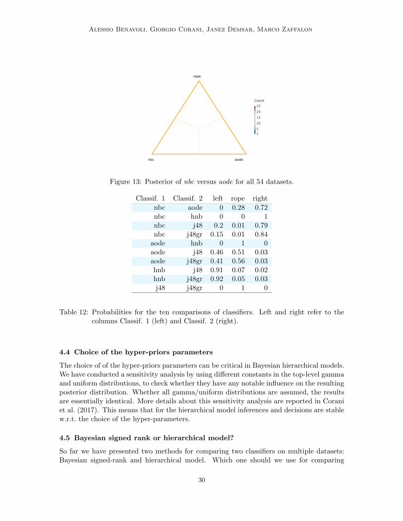
Alessio Benavoli, Giorgio Corani, Janez Demsar, Marco Zaffalon
1
20
10
15
25
5
Count
rope
aodenbc
Figure 13: Posterior of nbc versus aode for all 54 datasets.
Classif. 1 Classif. 2 left rope right
nbc aode 0 0.28 0.72nbc hnb 0 0 1nbc j48 0.2 0.01 0.79nbc j48gr 0.15 0.01 0.84
aode hnb 0 1 0aode j48 0.46 0.51 0.03aode j48gr 0.41 0.56 0.03hnb j48 0.91 0.07 0.02hnb j48gr 0.92 0.05 0.03j48 j48gr 0 1 0
Table 12: Probabilities for the ten comparisons of classifiers. Left and right refer to thecolumns Classif. 1 (left) and Classif. 2 (right).
4.4 Choice of the hyper-priors parameters
The choice of of the hyper-priors parameters can be critical in Bayesian hierarchical models.We have conducted a sensitivity analysis by using different constants in the top-level gammaand uniform distributions, to check whether they have any notable influence on the resultingposterior distribution. Whether all gamma/uniform distributions are assumed, the resultsare essentially identical. More details about this sensitivity analysis are reported in Coraniet al. (2017). This means that for the hierarchical model inferences and decisions are stablew.r.t. the choice of the hyper-parameters.
4.5 Bayesian signed rank or hierarchical model?
So far we have presented two methods for comparing two classifiers on multiple datasets:Bayesian signed-rank and hierarchical model. Which one should we use for comparing
30
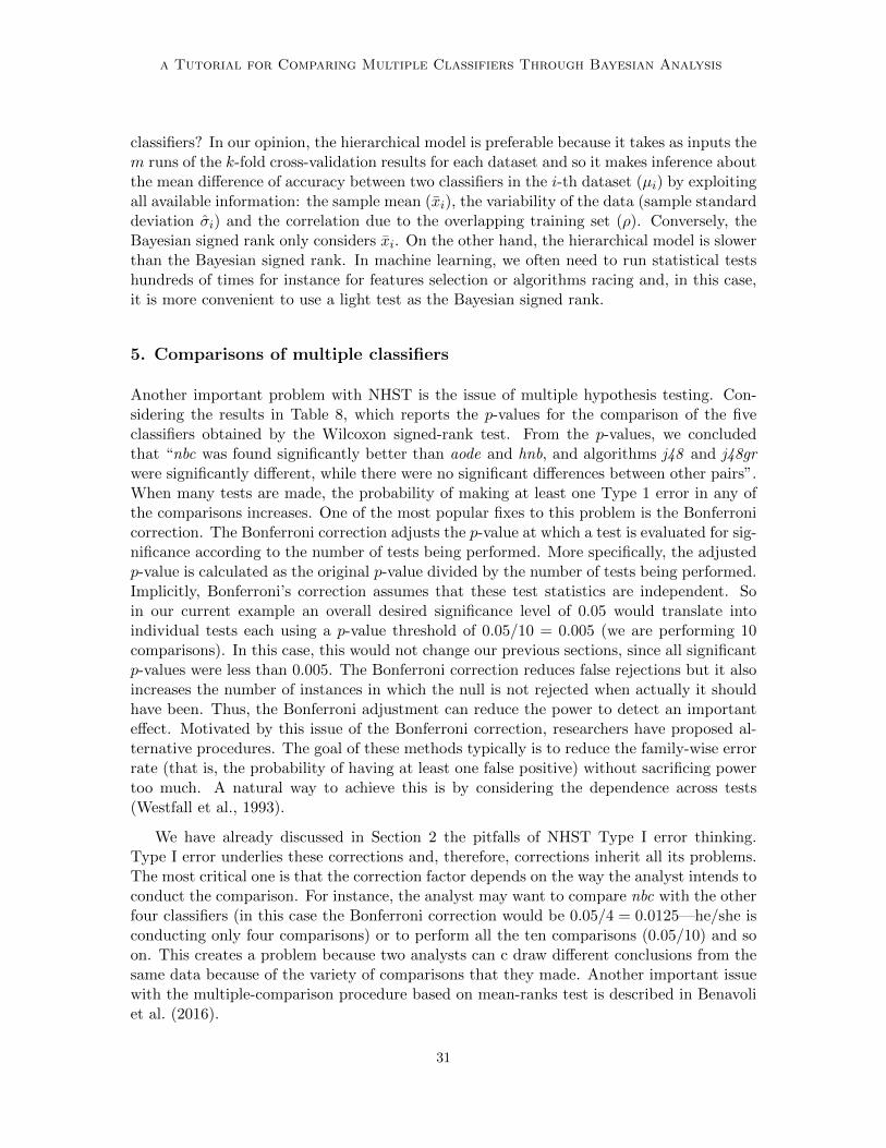
a Tutorial for Comparing Multiple Classifiers Through Bayesian Analysis
classifiers? In our opinion, the hierarchical model is preferable because it takes as inputs them runs of the k-fold cross-validation results for each dataset and so it makes inference aboutthe mean difference of accuracy between two classifiers in the i-th dataset (µi) by exploitingall available information: the sample mean (xi), the variability of the data (sample standarddeviation σi) and the correlation due to the overlapping training set (ρ). Conversely, theBayesian signed rank only considers xi. On the other hand, the hierarchical model is slowerthan the Bayesian signed rank. In machine learning, we often need to run statistical testshundreds of times for instance for features selection or algorithms racing and, in this case,it is more convenient to use a light test as the Bayesian signed rank.
5. Comparisons of multiple classifiers
Another important problem with NHST is the issue of multiple hypothesis testing. Con-sidering the results in Table 8, which reports the p-values for the comparison of the fiveclassifiers obtained by the Wilcoxon signed-rank test. From the p-values, we concludedthat “nbc was found significantly better than aode and hnb, and algorithms j48 and j48grwere significantly different, while there were no significant differences between other pairs”.When many tests are made, the probability of making at least one Type 1 error in any ofthe comparisons increases. One of the most popular fixes to this problem is the Bonferronicorrection. The Bonferroni correction adjusts the p-value at which a test is evaluated for sig-nificance according to the number of tests being performed. More specifically, the adjustedp-value is calculated as the original p-value divided by the number of tests being performed.Implicitly, Bonferroni’s correction assumes that these test statistics are independent. Soin our current example an overall desired significance level of 0.05 would translate intoindividual tests each using a p-value threshold of 0.05/10 = 0.005 (we are performing 10comparisons). In this case, this would not change our previous sections, since all significantp-values were less than 0.005. The Bonferroni correction reduces false rejections but it alsoincreases the number of instances in which the null is not rejected when actually it shouldhave been. Thus, the Bonferroni adjustment can reduce the power to detect an importanteffect. Motivated by this issue of the Bonferroni correction, researchers have proposed al-ternative procedures. The goal of these methods typically is to reduce the family-wise errorrate (that is, the probability of having at least one false positive) without sacrificing powertoo much. A natural way to achieve this is by considering the dependence across tests(Westfall et al., 1993).
We have already discussed in Section 2 the pitfalls of NHST Type I error thinking.Type I error underlies these corrections and, therefore, corrections inherit all its problems.The most critical one is that the correction factor depends on the way the analyst intends toconduct the comparison. For instance, the analyst may want to compare nbc with the otherfour classifiers (in this case the Bonferroni correction would be 0.05/4 = 0.0125—he/she isconducting only four comparisons) or to perform all the ten comparisons (0.05/10) and soon. This creates a problem because two analysts can c draw different conclusions from thesame data because of the variety of comparisons that they made. Another important issuewith the multiple-comparison procedure based on mean-ranks test is described in Benavoliet al. (2016).
31
Alessio Benavoli, Giorgio Corani, Janez Demsar, Marco Zaffalon
How do we manage the problem of multiple hypothesis testing in Bayesian analysis?Paraphrasing Gelman et al. (2012): “in Bayesian analysis we usually do not have to worryabout multiple comparisons. The reason is that we do not worry about Type I error,because the null hypothesis is hardly believable to be true.” How does Bayesian Analysismitigate false alarms? Gelman et al. (2012) suggest using multilevel analysis (in our casea hierarchical Bayesian model on multiple classifiers). Multilevel models perform partialpooling; they shift estimates toward each other. This means that the comparisons of theclassifiers are more conservative, in the sense that intervals for comparisons are more likelyto include zero. This may be a direction to pursue in future research. In this paper, weinstead mitigate false alarms through the rope. The rope mitigates false alarms because itdecreases the asymptotic false alarm rate (Kruschke, 2013).
6. Software and available Bayesian tests
All the tests that we have presented in this paper are available in R and Python code at
https://github.com/BayesianTestsML/tutorial/.
Moreover, the code that is necessary to replicate all the analyses we performed in this paperis also available at the above URL in form of Ipython notebooks (implemented in Pythonand Julia). The software is open source and that can be freely used, changed, and shared(in modified or unmodified form).
Machine learning researchers may be interested in using other Bayesian tests besidesthe ones we have discussed in this paper. General Bayesian parametric tests can be foundin Kruschke (2015) (together with R code) and also in Gelman et al. (2013). We havespecialized some of these tests to the case of correlated data, such as the Bayesian correlatedt-test (Corani and Benavoli, 2015) discussed in Section 3. We have also implemented severalBayesian nonparametric tests for comparing algorithms: Bayesian rank test (Benavoli et al.,2015b), Friedman test (Benavoli et al., 2015a) and tests that account for censored data(Mangili et al., 2015). Finally, we have developed an extension of the Bayesian sign test tocompare algorithms taking into account multiple measures at the same time (accuracy andcomputational time for instance) (Benavoli and Campos, 2015). For the analysis of multipledata sets, another approach has been proposed by Lacoste et al. (2012) that models eachdata set as an independent Bernoulli trial. The two possible outcomes of the Bernoulli trialare the first classifier being more accurate than the second or vice versa. This approachyields the posterior probability of the first classifier being more accurate than the secondclassifier on more than half of the q data sets. A shortcoming is that its conclusions applyonly to the q available data sets without generalizing to the whole population of data sets
7. Conclusions
We discourage the use of frequentist null hypothesis significance tests (NHST) in machinelearning and, in particular, for comparison of the performance of classifiers. In this, wefollow the current trends in other scientific areas. For instance, the journal of Basic andApplied Social Psychology, has banned the use of NHSTs and related statistical proce-dures (Trafimow and Marks, 2015). We believe that also in machine learning is time tomove on from NHST and p-values.
32
a Tutorial for Comparing Multiple Classifiers Through Bayesian Analysis
In this paper, we have discussed how Bayesian analysis can be employed instead ofNHST. In particular, we have presented three Bayesian tests: Bayesian correlated t-test,Bayesian signed rank test and a Bayesian hierarchical model that can be used for comparingthe performance of classifiers and that solve the drawbacks of the frequentist tests. Allthe code of these tests is freely available and so researchers can already use these testsfor their analysis. In this paper, we have mainly discussed the use of Bayesian tests forcomparing the performance of algorithms. However, in machine learning, NHST statisticaltests are also employed inside the algorithms. For instance, nonparametric tests are used inracing algorithms, independence tests are used to learn the structure of Bayesian networks,etcetera. Bayesian tests can be used to replace all NHST tests because of their advantages(for instance, Bayesian tests can assess whether two algorithms are similar through the useof the rope (Benavoli et al., 2015a)).
Acknowledgements
Research partially supported by the Swiss NSF grant no. IZKSZ2 162188.
References
Murray Aitkin. Posterior Bayes factors. Journal of the Royal Statistical Society. Series B(Methodological), pages 111–142, 1991.
M.J. Bayarri and James O Berger. Hypothesis Testing and Model Uncertainty. In BayesianTheory and Applications, pages 365–394. OUP Oxford, 2013.
Alessio Benavoli and Cassio P. Campos. Advanced Methodologies for Bayesian Networks:Second International Workshop, AMBN 2015, Yokohama, Japan, November 16-18, 2015.Proceedings, chapter Statistical tests for joint analysis of performance measures. SpringerInternational Publishing, Cham, 2015.
Alessio Benavoli, Francesca Mangili, Giorgio Corani, Marco Zaffalon, and Fabrizio Ruggeri.A Bayesian Wilcoxon signed-rank test based on the Dirichlet process. In Proceedings ofthe 30th International Conference on Machine Learning (ICML 2014), pages 1–9, 2014.
Alessio Benavoli, Giorgio Corani, Francesca Mangili, and Marco Zaffalon. A Bayesian non-parametric procedure for comparing algorithms. In Proceedings of the 31th InternationalConference on Machine Learning (ICML 2015), pages 1–9, 2015a.
Alessio Benavoli, Francesca Mangili, Fabrizio Ruggeri, and Marco Zaffalon. ImpreciseDirichlet process with application to the hypothesis test on the probability that X≤Y.Journal of Statistical Theory and Practice, 9(3):658–684, 2015b.
Alessio Benavoli, Giorgio Corani, and Francesca Mangili. Should we really use post-hoctests based on mean-ranks? Journal of Machine Learning Research, 17(5):1–10, 2016.
James O. Berger. Statistical Decision Theory and Bayesian Analysis. Springer Series inStatistics, New York, 1985.
33
Alessio Benavoli, Giorgio Corani, Janez Demsar, Marco Zaffalon
James O. Berger and Luis R Pericchi. The intrinsic Bayes factor for model selection andprediction. Journal of the American Statistical Association, 91(433):109–122, 1996.
James O. Berger and Thomas Sellke. Testing a point null hypothesis: The irreconcilability ofp-values and evidence. Journal of the American statistical Association, 82(397):112–122,1987.
James O. Berger, E. Moreno, L. R. Pericchi, M. J. Bayarri, Bernardo, et al. An overviewof robust Bayesian analysis. Test, 3(1):5–124, 1994.
Jose M Bernardo and Adrian FM Smith. Bayesian theory, volume 405. Wiley Chichester,2009.
Christopher Bishop. Pattern Recognition and Machine Learning. Springer, 2007.
Remco R Bouckaert. Choosing between two learning algorithms based on calibrated tests.In Proceedings of the 20th International Conference on Machine Learning (ICML-03),pages 51–58, 2003.
Bob Carpenter, Daniel Lee, Marcus A Brubaker, Allen Riddell, Andrew Gelman, BenGoodrich, Jiqiang Guo, Matt Hoffman, Michael Betancourt, and Peter Li. Stan: Aprobabilistic programming language. Journal of Statistical Software, in press, 2016.
Giorgio Corani and Alessio Benavoli. A Bayesian approach for comparing cross-validatedalgorithms on multiple data sets. Machine Learning, 100(2):285–304, 2015. doi: 10.1080/s10994-015-5486-z.
Giorgio Corani, Alessio Benavoli, Janez Demsar, Francesca Mangili, and Marco Zaffalon.Statistical comparison of classifiers through Bayesian hierarchical modelling. MachineLearning in press, 2017. doi: 10.1007/s10994-017-5641-9.
Janez Demsar. Statistical comparisons of classifiers over multiple data sets. Journal ofMachine Learning Research, 7:1–30, 2006.
Janez Demsar. On the appropriateness of statistical tests in machine learning. In Workshopon Evaluation Methods for Machine Learning in conjunction with ICML, 2008.
James Dickey. Scientific reporting and personal probabilities: Student’s hypothesis. Journalof the Royal Statistical Society. Series B (Methodological), pages 285–305, 1973.
Thomas G. Dietterich. Approximate statistical tests for comparing supervised classificationlearning algorithms. Neural Computation, 10:1895–1924, 1998.
Ward Edwards, Harold Lindman, and Leonard J Savage. Bayesian statistical inference forpsychological research. Psychological review, 70(3):193, 1963.
Andrew Gelman. Prior distributions for variance parameters in hierarchical models (com-ment on article by browne and draper). Bayesian analysis, 1(3):515–534, 2006.
34
a Tutorial for Comparing Multiple Classifiers Through Bayesian Analysis
Andrew Gelman, Jennifer Hill, and Masanao Yajima. Why we (usually) don’t have toworry about multiple comparisons. Journal of Research on Educational Effectiveness, 5(2):189–211, 2012.
Andrew Gelman, John B Carlin, Hal S Stern, David B Dunson, Aki Vehtari, and Donald BRubin. Bayesian Data Analysis. CRC press, 2013.
Andrew Gelman, John B Carlin, Hal S Stern, and Donald B Rubin. Bayesian Data Analysis,volume 2. Taylor & Francis, 2014.
Myles Hollander, Douglas A Wolfe, and Eric Chicken. Nonparametric Statistical Methods,volume 751. John Wiley & Sons, 2013.
Miguel A Juarez and Mark FJ Steel. Model-based clustering of non-gaussian panel databased on skew-t distributions. Journal of Business & Economic Statistics, 28(1):52–66,2010.
Robert E Kass and Adrian E Raftery. Bayes factors. Journal of the American StatisticalAssociation, 90(430):773–795, 1995.
John K. Kruschke. Bayesian data analysis. Wiley Interdisciplinary Reviews: CognitiveScience, 1(5):658–676, 2010.
John K. Kruschke. Bayesian estimation supersedes the t-test. Journal of ExperimentalPsychology: General, 142(2):573, 2013.
John K. Kruschke. Doing Bayesian Data Analysis: A Tutorial with R, Jags and Stan.Academic Press, 2015.
John K. Kruschke and Torrin M Liddell. The Bayesian New Statistics: Two HistoricalTrends Converge. Available at SSRN 2606016, 2015.
Alexandre Lacoste, Francois Laviolette, and Mario Marchand. Bayesian comparison ofmachine learning algorithms on single and multiple datasets. In Proc.of the FifteenthInternational Conference on Artificial Intelligence and Statistics (AISTATS-12), pages665–675, 2012.
Bruno Lecoutre and Jacques Poitevineau. The Significance Test Controversy Revisited.Springer, 2014.
Francesca Mangili, Alessio Benavoli, Cassio P. de Campos, and Marco Zaffalon. Reliablesurvival analysis based on the Dirichlet Process. Biometrical Journal, 57:10021019, 2015.
Kevin P Murphy. Machine Learning: a Probabilistic Perspective. MIT press, 2012.
Claude Nadeau and Yoshua Bengio. Inference for the generalization error. Machine Learn-ing, 52(3):239–281, 2003.
Steven L. Salzberg. On comparing classifiers: Pitfalls to avoid and a recommended approach.Data Mining and Knowledge Discovery, 1:317–328, 1997.
35

Alessio Benavoli, Giorgio Corani, Janez Demsar, Marco Zaffalon
Zbynek Sidak, Pranab Sen, and Jaroslav Hajek. Theory of Rank Tests. Probability andMathematical Statistics. Elsevier Science, 1999.
David Trafimow and Michael Marks. Editorial. Basic and applied social psychology, 37(1):1–2, 2015.
Peter Walley. Inferences from multinomial data: learning about a bag of marbles. Journalof the Royal Statistical Society. Series B (Methodological), 58(1):3–57, 1996.
Ronald L Wasserstein and Nicole A Lazar. The ASA’s statement on p-values: context,process, and purpose. The American Statistician, (just-accepted):00–00, 2016.
Peter H Westfall, S Stanley Young, and S Paul Wright. On adjusting p-values for multi-plicity. Biometrics, 49(3):941–945, 1993.
Ian H Witten, Eibe Frank, and Mark Hall. Data Mining: Practical Machine Learning Toolsand Techniques (third edition). Morgan Kaufmann, 2011.
36