Time Preference and the Distributions of Wealth and

Income

Richard M. H. Suen�

This Version: February 2010

Abstract

This paper presents a dynamic competitive equilibrium model with heterogeneous time pref-

erences that can account for the observed patterns of wealth and income inequality in the United

States. This model generalizes the standard neoclassical growth model by including (i) a demand

for status by the consumers and (ii) human capital formation. The �rst feature prevents the

wealth distribution from collapsing into a degenerate distribution. The second feature generates

a strong positive correlation between earnings and wealth across agents. A calibrated version of

this model succeeds in replicating the wealth and income distributions of the United States.

Keywords: Inequality, Heterogeneity, Time Preference, Human Capital

JEL classi�cation: D31, E21, O15.

�Department of Economics, Sproul Hall, University of California, Riverside CA 92521-0427. Email:richard.suen@ucr.edu. Tel.: (951) 827-1502. Fax: (951) 827-5685.

1

1 Introduction

Empirical studies show that individuals do not discount future values at the same rate.1 Since

individuals� investment decisions are strongly a¤ected by the way they discount the future, this

type of heterogeneity would naturally lead to inequality in wealth and income. In this paper, we

present a dynamic competitive equilibrium model with heterogeneous time preferences that can

account for the observed patterns of wealth and income inequality in the United States.

It is well known that standard dynamic competitive equilibrium models have di¢ culty in gen-

erating realistic wealth distribution based on heterogeneous time preferences alone. Speci�cally,

when consumers have time-additive separable preferences and di¤erent constant discount factors,

all the wealth in the model economy will eventually be concentrated in the hands of the most pa-

tient consumers. This classic result is �rst conjectured by Ramsey (1928) and formally proved by

Becker (1980). The current study begins by showing that Becker�s result cannot be extended to the

case where consumers derive utility from both consumption and wealth. In our baseline model, we

adopt the same economic environment as in Becker (1980), which features a neoclassical production

technology, a complete set of competitive markets, consumers with heterogeneous time preferences

and a borrowing constraint. The only modi�cation we make is the inclusion of wealth in consumers�

preferences. It is formally shown that the baseline model possesses a unique stationary equilibrium

in which every consumer owns a positive amount of wealth. A calibrated version of the baseline

model is able to replicate some key features of the wealth distribution in the United States. In

particular, it is able to generate a large group of wealth-poor consumers and a very small group of

extremely wealthy ones. However, the baseline model falls short in explaining income inequality.

This problem remains even if we allow for endogenous labor supply. To overcome this problem, we

extend the baseline model by introducing human capital formation. The main idea of this extension

is that more patient consumers are more willing to invest in their wealth and human capital than

less patient ones. A higher level of human capital then leads to a higher level of future earnings

for the more patient consumers. This gives rise to a strong positive correlation between wealth

and earnings which is essential in accounting for wealth and income inequality simultaneously. A

calibrated version of this model succeeds in replicating the distributions of wealth and income in

1See, for instance, Hausman (1979), Lawrance (1991), Samwick (1998), and Warner and Pleeter (2001). A detailedreview of this literature can be found in Frederick, et al. (2002) Section 6.

2

the United States.

In the current study, we assume that consumers value wealth directly in their preferences. This

assumption has long been used in economic studies. In an early paper, Kurz (1968) introduces this

type of preferences into the optimal growth model and explores the long-run properties of the model.

Zou (1994) interprets this type of preferences as re�ecting the �capitalist spirit,�which refers to

the tendency of treating wealth acquisition as an end in itself rather than a means of satisfying

material needs. Cole, et al. (1992) suggest that this type of preferences can serve as a reduced-

form speci�cation to capture people�s concern for their relative wealth position or status within

society. Subsequent studies have followed these traditions and interpreted this type of preferences

as embodying the spirit of capitalism or re�ecting the demand for wealth-induced social status.

There is now a growing literature that explores the implications of capitalist spirit on a wide

range of issues, including asset pricing, economic growth, the e¤ects of monetary policy and wealth

inequality.2 Among the existing studies, Luo and Young (2009) is most relevant to this paper.

These authors consider an economy in which consumers share the same time preference, concern

about their status in the economy and face uninsurable idiosyncratic labor income risk. They �nd

that the demand for social status is a force that tends to reduce wealth inequality. This result is

also observed in our model. First, the equilibrium wealth distribution is no longer degenerate once

we introduce the demand for social status into Becker�s model. Second, in the quantitative analysis,

we �nd that wealth inequality decreases as we increase the coe¢ cient that controls the demand for

status.

Our baseline model can yield a non-degenerate wealth distribution because adding a demand for

status fundamentally changes consumers�investment behavior. In the original Becker (1980) model,

a consumer facing a constant interest rate invests according to the following rules: accumulate wealth

inde�nitely if the interest rate exceeds his rate of time preference, deplete his wealth until it reaches

zero if the opposite is true, and maintain a constant positive level of wealth if the two rates coincide.

Since no one can accumulate wealth inde�nitely in a stationary equilibrium, the equilibrium interest

rate is determined by the lowest rate of time preference among the consumers. It follows from the

2Studies that explore the implications of capitalist spirit on asset pricing include Bakshi and Chen (1996), andBoileau and Braeu (2007) among others. Studies on economic growth include Zou (1994) and Smith (1999) amongothers. Gong and Zou (2001), Chang and Tsai (2003) and Chen and Guo (2009) examine the e¤ects of monetarypolicy on capital accumulation and economic growth in the presence of social-status concern. Finally, Luo and Young(2009) explore the implications of capitalist spirit on wealth inequality.

3

above rules that consumers with a higher rate of time preference would end up having zero wealth.

In contrast, a status-seeking consumer is willing to hold a constant positive amount of wealth even

if the equilibrium interest rate is lower than his rate of time preference. The consumer is willing to

do so because holding a positive amount of wealth also satis�es his need for status. The demand

for status in e¤ect creates some additional rewards from investment other than the market rate of

return. These additional rewards keep consumers from depleting their wealth to zero.

How important is the demand for status to our quantitative results? First, the demand for

status prevents the wealth distribution from collapsing into a degenerate distribution. This allows

us to explore the implications of heterogeneous time preferences on wealth and income inequality.

Our quantitative results show that the extent of wealth inequality is strongly in�uenced by the

coe¢ cient that controls the demand for status. However, this is not the only decisive factor: the

distribution of discount factor plays an equally important role in determining wealth inequality.

Our baseline results also show that the demand for status cannot generate a substantial degree of

income inequality. In the model with human capital, the demand for status does not play any role

in determining the distributions of hours and labor earnings. These distributions are completely

determined by two factors: (i) the distribution of discount factor, and (ii) the parameters in the

human capital accumulation process which are chosen based on empirical �ndings.

This paper is complementary to two di¤erent groups of studies. The �rst group of studies at-

tempt to explain the observed patterns of income and wealth inequality by considering di¤erent

versions of the heterogeneous-agent model à la Huggett (1993) and Aiyagari (1994). In this type

of models, income inequality is driven by the exogenous labor income risk, and wealth inequality

is largely determined by consumers�precautionary saving motive. It is well-documented that the

standard Aiyagari-Huggett model has di¢ culty in generating realistic wealth inequality.3 Krusell

and Smith (1998) show that introducing heterogeneous time preferences can signi�cantly improve

the Aiyagari-Huggett model in this regard. To obtain this result, these authors assume that con-

sumers�subjective discount factors are stochastic in nature. The second group of studies are mainly

theoretical studies that establish a non-degenerate wealth distribution in the presence of heteroge-

neous time preferences. Lucas and Stokey (1984) and Boyd (1990) show that Becker�s result is no

longer valid when consumers have recursive preferences. Sarte (1997) establishes the existence of a

3See Quadrini and Ríos-Rull (1997), and Castañeda, et al. (2003) for detailed discussions of this problem.

4

non-degenerate wealth distribution by introducing a progressive tax structure into Becker�s model.

More recently, Espino (2005) establishes this result by assuming that consumers have private in-

formation over an idiosyncratic preference shock. Sorger (2002, 2008) show that Becker�s result

cannot be extended to the case where consumers are strategic players, rather than price-takers, in

the capital market.

The rest of this paper is organized as follows. Section 2 describes the baseline model environment,

presents the main theoretical results and evaluates the quantitative relevance of this model. Section

3 extends the baseline model by including endogenous labor supply. Section 4 presents the extension

with human capital formation. Section 5 concludes.

2 The Baseline Model

2.1 Preferences

Consider an economy inhabited by a large number of in�nitely lived agents. The size of population

is constant over time and is given by N: Each agent is indexed by a subjective discount factor �i;

for i 2 f1; 2; :::; Ng : The discount factors are ranked according to 1 > �1 � �2 � : : : � �N > 0:

There is a single commodity in this economy which can be used for consumption and investment.

All agents have preferences over streams of consumption and social status, which can be represented

by1Xt=0

�tiu (cit; sit) ; (1)

where cit and sit denote the consumption and social status of agent i at time t: The period utility

function u : R2+ ! R is assumed to be identical for all agents and have the following properties:

Assumption A1 The function u (c; s) is twice continuously di¤erentiable, strictly increasing and

strictly concave in (c; s) : It also satis�es the Inada condition for consumption, i.e., limc!0

uc (c; s) =1;

where uc (c; s) is the partial derivative with respect to c:

Assumption A2 The function u (c; s) is homogeneous of degree 1� �; with � > 0:

Assumption A2 is imposed to ensure the existence of balanced growth equilibria. Under this

assumption, the partial derivatives uc (c; s) and us (c; s) are both homogeneous of degree ��: We

5

can then de�ne a function h : R+ ! R according to

h (z) � us (z; 1)

uc (z; 1): (2)

Under Assumption A1, the function h (z) is continuously di¤erentiable and non-negative. We now

impose some additional assumptions on this function.

Assumption A3 The function h (z) de�ned by (2) is strictly increasing and satis�es h (0) = 0

and limz!1

h (z) =1:

It is straightforward to check that if ucs (c; s) � 0 then h (z) is strictly increasing. The converse,

however, is not true in general. In other words, Assumption A3 does not preclude the possibility of

having a negative cross-derivative for some values of c and s.

All three assumptions stated above are satis�ed by the following functional forms which are

commonly used in the existing literature,

u (c; s) =1

1� ��c1�� + �s1��

�; (3)

with � > 0 and � > 0; and

u (c; s) =1

1� �

h�c + (1� �) s

i 1�� ; (4)

with � > 0; � 2 (0; 1) and < 1:4

2.2 The Agents�Problem

In each period, each agent is endowed with one unit of time which is supplied inelastically to the

market. The agents receive labor income from work and interest income from previous savings. All

savings are held in the form of physical capital, which is the only asset in this economy. As in

Becker (1980), the agents are not allowed to borrow so that capital holdings must be non-negative

4The additively separable utility function is used in Zou (1994), Gong and Zou (2001), and Luo and Young (2009)among others. The non-separable utility function is used in Boileau and Braeu (2007). Luo and Young (2009) alsoconsider a Stone-Geary type of preferences over status. We do not consider this in here because it is inconsistent withbalanced growth equilibria.

6

in each period. An agent�s social status is measured by the level of wealth owned by the agent at

the beginning of the current period. Speci�cally, this means

sit = kit; for all t � 0;

where kit is the stock of capital owned by agent i at the beginning of time t: The same speci�cation

of status is also used in Zou (1994), Bakshi and Chen (1996) and Luo and Young (2009) among

others.

Given a sequence of wages and rental rates, the agents� problem is to choose sequences of

consumption and capital so as to maximize their discounted lifetime utility, subject to sequences

of budget constraints and borrowing constraints. Let wt and rt be the market wage rate and the

rental rate of capital at time t: Formally, agent i�s problem is given by

maxfcit;kit+1g1t=0

1Xt=0

�tiu (cit;sit)

subject to

cit + kit+1 � (1� �) kit = wt + rtkit; (5)

kit+1 � 0;

sit = kit;

and ki0 > 0 given.5 The parameter � 2 (0; 1) is the depreciation rate of capital.

The agents�optimal choices are completely characterized by the sequential budget constraint in

(5), and the Euler equation

uc (cit;kit) � �i [us (cit+1;kit+1) + (1 + rt+1 � �)uc (cit+1;kit+1)] ; (6)

which holds with equality if kit+1 > 0: For a status-seeking agent, additional investment in the

current period raises future utility by (i) generating more resources for future consumption, and

(ii) promoting his future status. The second e¤ect is captured by the term us (cit+1;kit+1) in the

5 In the theoretical and quantitative analyses, we focus on balanced-growth equilibria which are independent of theinitial conditions. Thus, the initial distribution of capital across agents is irrelevant to our analyses.

7

Euler equation. If status is not valued, then us (cit+1;kit+1) = 0 and the Euler equation in (6) will

be identical to the one in Becker (1980).

2.3 Production

Output is produced according to a standard neoclassical production function:

Yt = F (Kt; XtLt) ;

where Yt denote aggregate output at time t, Kt is aggregate capital, Lt is aggregate labor and Xt is

the level of labor-augmenting technology. We will refer to bLt � XtLt as the e¤ective unit of labor.

The technological factor is assumed to grow at a constant exogenous rate so that Xt � t for all t;

where � 1 is the exogenous growth factor and X0 is normalized to one. The production function

F : R2+ ! R+ is assumed to have all the usual properties which are summarized below.

Assumption A4 The production function F�K; bL� is twice continuously di¤erentiable, strictly

increasing and strictly concave in each argument. It exhibits constant returns to scale and satis�es

the following conditions: F�0; bL� = 0 for all bL � 0; F (K; 0) = 0 for allK � 0; lim

K!0FK

�K; bL� =1

and limK!1

FK

�K; bL� = 0:

Because of the constant-returns-to-scale assumption, we can focus on a representative �rm whose

problem is given by

maxKt;Lt

fF (Kt; XtLt)� wtLt � rtKtg :

The solution of this problem is completely characterized by the �rst-order conditions:

wt = XtFbL (Kt; XtLt) = XtFbL�bkt; 1�

and

rt = FK (Kt; XtLt) = FK

�bkt; 1� ;where bkt � Kt= (XtLt) is the amount of capital per e¤ective unit of labor at time t:

8

2.4 Competitive Equilibrium

Let ct = (c1t; c2t; :::; cNt) denote a distribution of consumption across agents at time t and kt =

(k1t; k2t; :::; kNt) be a distribution of capital at time t. A competitive equilibrium consists of se-

quences of distributions of consumption and capital, fct;ktg1t=0 ; sequences of aggregate inputs,

fKt; Ltg1t=0 ; and sequences of prices, fwt; rtg1t=0 ; so that

(i) Given the prices fwt; rtg1t=0 ; the sequences fcit; kitg1t=0 solve agent i�s problem.

(ii) In each period t � 0; given the prices wt and rt; the aggregate inputs Kt and Lt solve the

representative �rm�s problem.

(iii) All markets clear in every period, so that for each t � 0;

Kt =NXi=1

kit;

andNXi=1

cit +Kt+1 � (1� �)Kt = F (Kt; XtN) :

In this paper, we con�ne our attention to balanced-growth equilibria. Formally, a set of sequences

S = fct;kt;Kt; Lt; wt; rtg1t=0 is called a balanced-growth equilibrium if the following conditions are

satis�ed:

(i) S is a competitive equilibrium as de�ned above.

(ii) The rental rate of capital is stationary over time, i.e., rt = r� for all t:

(iii) Individual consumption and capital, aggregate capital and the wage rate are all growing at

the same constant rate. In particular, the common growth factor is � 1:

2.5 Theoretical Results

The main objective of this subsection is to show that, under certain conditions, the baseline model

possesses a unique balanced-growth equilibrium in which all agents hold a strictly positive amount

of capital. Before stating the formal theorem, we need to introduce some additional notations.

9

A balanced-growth equilibrium for this economy is characterized by a constant rental rate r�

which clears the capital market. Once the equilibrium rental rate is determined, all other variables

in a balanced-growth equilibrium can be uniquely determined. Thus it su¢ ces to establish the

existence and uniqueness of r�. To achieve this, we �rst formulate the supply and demand for

capital as a function of r:

Denote by bkd (r) the amount of capital per e¤ective unit of labor that the representative �rmdesires when the rental rate is r: The function bkd (r) is implicitly de�ned by the condition:

r = FK

�bkd; 1� : (7)

Under Assumption A4, the function bkd : R++ ! R+ is continuously di¤erentiable and strictly

decreasing. Moreover, bkd (r) approaches in�nity as r tends to zero from the right and approaches

zero as r tends to in�nity. If r is an equilibrium rental rate, then the equilibrium wage rate at time

t is uniquely determined by wt = t bw (r) ; wherebw (r) = FbL

�bkd (r) ; 1� : (8)

Next, we consider the supply side of the capital market. Along any balanced-growth equilibrium

path, individual consumption and capital can be expressed as cit = tbci and kit = tbki; where bci andbki are stationary over time. The values of bci and bki are determined by agent i�s budget constraintand the Euler equation for consumption. In a balanced-growth equilibrium, the agent�s budget

constraint becomes

bci = bw (r) + �r � b��bki; (9)

where b� � � 1 + � � �: Under Assumptions A2 and A3, the Euler equation can be expressed as

�

�i� (1� �)� r � h

�bcibki�; (10)

which holds with equality if bki > 0: By Assumption A3, we have h (z) � 0 for all z � 0: In the aboveequation, z is the consumption-capital ratio for agent i, which must be non-negative in equilibrium.

Thus, the Euler equation is valid only for r � bri; where bri � �=�i � (1� �) > 0: This essentially

10

imposes an upper bound on the equilibrium rental rate, which is minifbrig = br1:6 For any r 2 (0; br1) ;

it is never optimal for any agent i to choose a zero value for bki:7 It follows that the Euler equation forconsumption will always hold with equality in a balanced-growth equilibrium. Combining equations

(9) and (10) gives �

�i� (1� �)� r = h

� bw (r)bki + r � b�� ; (11)

which determines the relationship between bki and r: Formally, this can be expressed asbki = gi (r) ;

where gi : (0; bri)! R+ is a continuously di¤erentiable function implicitly de�ned by (11).

Denote by bks (r) the aggregate supply of capital per e¤ective unit of labor when the rental rateis r 2 (0; br1) : Formally, this is de�ned as

bks (r) = 1

N

NXi=1

gi (r) :

Since each gi (r) is continuous on (0; br1) ; the function bks (r) is also continuous on this range. Abalanced-growth equilibrium exists if there exists at least one value r� within the range (0; br1) thatsolves the capital market equilibrium condition:

bkd (r) = bks (r) : (12)

Once r� is determined, all other variables, including the cross-sectional distributions of consumption

and capital (ct;kt) ; the aggregate capital Kt and the wage rate wt, can be uniquely determined. If

there exists at most one such value of r�; then the balanced-growth equilibrium is unique.

We are now ready to state the main result of this section. Theorem 1 states the conditions under

which a unique balanced-growth equilibrium exists. The formal proof of this result can be found in

Appendix A.

6 If r exceeds br1; then the Euler equation will not be satis�ed for some agents and so r cannot be an equilibriumrental rate.

7To see this, suppose the contrary that some agent i chooses to have bki = 0 in a balanced-growth equilibrium.Then the right-hand side of (10) would become in�nite as lim

z!1h (z) =1 under Assumption A3. This clearly exceeds

the left-hand side of the inequality for any r 2 (0; br1) and hence gives rise to a contradiction.11

Theorem 1 Suppose Assumptions A1-A4 are satis�ed. Suppose the following condition holds

bkd �b�� > bks �b�� : (13)

Then there exists a unique balanced-growth equilibrium in which all agents hold a strictly positive

amount of capital. In addition, more patient agents would have more consumption and hold more

capital than less patient ones, i.e., �i > �j implies bci > bcj and bki > bkj :We now explain the intuitions behind Theorem 1. To facilitate comparison with the original

result in Becker (1980), we set = 1 for the moment. For each i 2 f1; 2; :::; Ng ; the parameter

�i � 1=�i � 1 is the rate of time preference for agent i: In a world where status is not valued, an

agent in a stationary equilibrium will invest according to the following rules: accumulate capital

inde�nitely if the e¤ective return from investment (r� � �) exceeds his rate of time preference,

deplete capital until it reaches zero if the e¤ective return is lower than his rate of time preference,

and maintain a constant positive capital stock if the two are equal. Since there is only one e¤ective

return from investment, it is not possible for agents with di¤erent rates of time preference to

maintain a constant capital stock simultaneously. At the same time, no one can accumulate capital

inde�nitely in a stationary equilibrium. Thus the e¤ective return must be equated to the lowest

rate of time preference among the agents. It follows that only the most patient agents will hold

a positive level of capital in the steady state, and that all other agents with a higher rate of time

preference will deplete their capital until it reaches zero.

Introducing a demand for status breaks this spell by creating some additional bene�ts of holding

capital. These additional bene�ts induce a change in consumers�investment behavior. In particular,

a status-seeking agent is willing to maintain a constant positive capital stock even if the e¤ective

return from investment is lower than his rate of time preference. This is made clear by the Euler

equation

�i � (r� � �) =us

�bci;bki�uc

�bci;bki� > 0;which implies �i > (r

� � �) for all i: The term on the right-hand side of the equation captures the

additional bene�ts of holding capital due to the demand for status. It is now possible to obtain a

non-degenerate capital distribution because agents with di¤erent rates of time preference can choose

12

a di¤erent value of bki based on the above equation. For impatient agents, they are willing to hold aconstant capital stock only if they are compensated by large bene�ts from status. Under the stated

assumptions, these bene�ts are diminishing in bki: Thus, less patient agents would choose a smallervalue of bki than more patient agents.

Condition (13) in Theorem 1 is imposed to ensure that the equilibrium rental rate r� is greater

than b�: According to (9), r� > � is both necessary and su¢ cient to guarantee that individual

consumption and capital holdings are positively correlated in the balanced-growth equilibrium.

2.6 Calibration

Our goal here is to evaluate the ability of the baseline model to replicate the observed patterns of

inequality in the United States. To achieve this, we have to �rst specify the form of the utility

function and the production function, and assign speci�c values to the model parameters. Some of

these values are chosen based on empirical �ndings. Others are chosen to match some real-world

targets. This details of this procedure are explained below.

Functional Forms and Parameters

In the numerical exercise, the production function is given by

F (K;XL) = K� (XL)1�� ;

with � 2 (0; 1) : The period utility function is assumed to be additively separable as in (3). In this

functional form, the parameter � captures the importance of social status in consumers�preferences.

The original Becker model corresponds to the case in which � = 0: The additively separable speci-

�cation is chosen for the following reasons. In the current model, individuals�investment decisions

are completely characterized by equation (11). Under the additively separable utility function, this

equation can be expressed as

�

�i� (1� �)� r = �

� bw (r)bki + r � b��� : (14)

13

Under the non-separable functional form in (4), this equation becomes

�

�i� (1� �)� r = 1� �

�

� bw (r)bki + r � b��1� : (15)

A direct comparison of these equations suggests that they can be made identical by a suitable choice

of parameter values. When this is imposed, all agents will have the same optimal investment rule

gi (r) under the two speci�cations of u (c; s). It follows that the equilibrium rental rate r� and

the wealth distribution will also be identical. This result can be stated formally as follows. Let

bc = (bc1; :::;bcN ) and bk = �bk1; :::;bkN� be the distributions of consumption and capital obtained underthe non-separable speci�cation in (4) with a common growth factor : Then the same distributions

can be obtained under an additively separable utility function with � = 1� ; � = (1� �) =�; and

a common growth factor e = �

1� :8 This result suggests that these two forms of utility function

are likely to yield quantitatively similar results in the balanced-growth equilibrium.9 We choose the

additively separable form because it involves fewer parameters.

The following parameter values are used in the quantitative exercise. The share of capital income

in total output (�) is 0.33. The growth rate of per-capita variables ( � 1) is 2.2 percent, which

is the average annual growth rate of real per-capita GDP in the United States over the period

1950-2000. The parameter � in the utility function is set to one, which is the same as in Luo

and Young (2009). The range of subjective discount factors is chosen based on the estimates in

Lawrance (1991). Using data from the Panel Study of Income Dynamics over the period 1974-1982,

Lawrance (1991) estimates that the average rate of time preference for households in the bottom

�fth percentile of the income distribution is 3.5 percent, after controlling for di¤erences in age,

educational level and race. This implies an average discount factor of 1/(1+0.035)=0.966 for these

households. The estimated rate of time preference for the richest �ve percent is 0.8 percent, which

corresponds to a discount factor of 0.992. In the benchmark scenario, we consider a hypothetical

population of 1,000 agents with discount factors uniformly distributed between 0.966 and 0.992.

This implies an average discount factor of 0.979. After presenting the benchmark results, we will

examine the e¤ects of changing the distribution of discount factors.

8 In the expression �

1� ; the parameter � is the one that appears in the non-separable utility function.9We stress that this �equivalence�result is valid only in the balanced-growth equilibrium. The two speci�cations

are likely to yield very di¤erent results along any transition path.

14

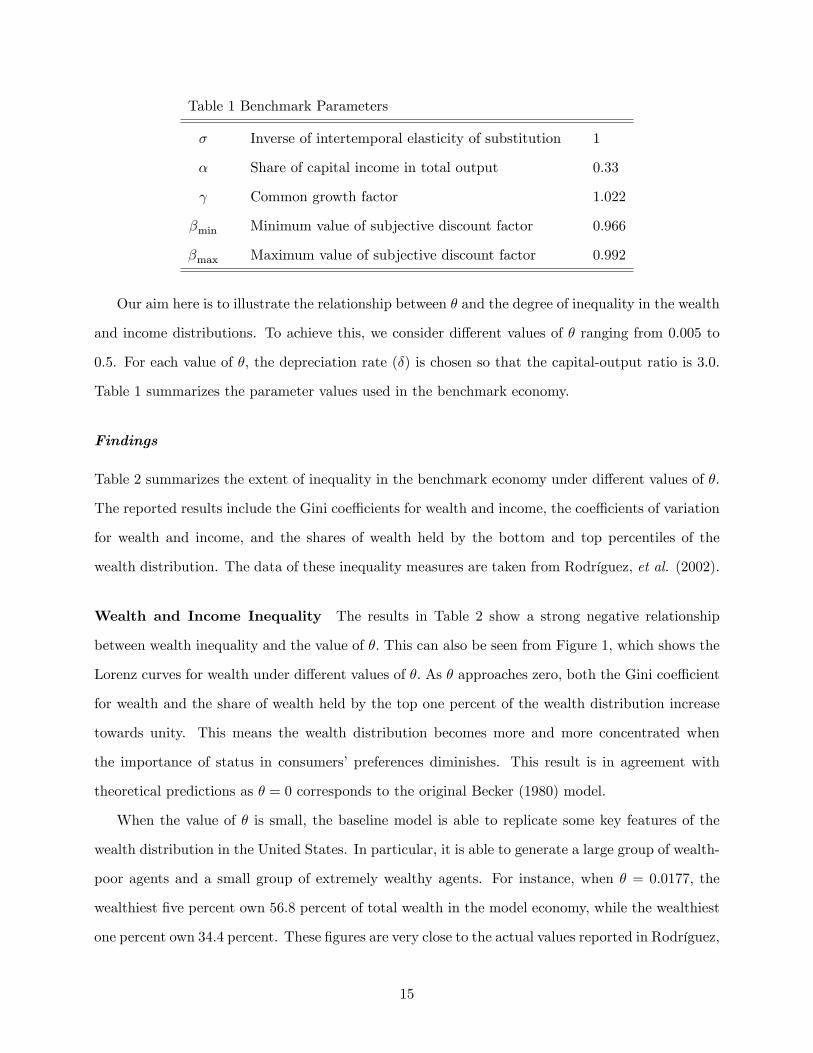
Table 1 Benchmark Parameters

� Inverse of intertemporal elasticity of substitution 1

� Share of capital income in total output 0.33

Common growth factor 1.022

�min Minimum value of subjective discount factor 0.966

�max Maximum value of subjective discount factor 0.992

Our aim here is to illustrate the relationship between � and the degree of inequality in the wealth

and income distributions. To achieve this, we consider di¤erent values of � ranging from 0.005 to

0.5. For each value of �; the depreciation rate (�) is chosen so that the capital-output ratio is 3.0.

Table 1 summarizes the parameter values used in the benchmark economy.

Findings

Table 2 summarizes the extent of inequality in the benchmark economy under di¤erent values of �:

The reported results include the Gini coe¢ cients for wealth and income, the coe¢ cients of variation

for wealth and income, and the shares of wealth held by the bottom and top percentiles of the

wealth distribution. The data of these inequality measures are taken from Rodríguez, et al. (2002).

Wealth and Income Inequality The results in Table 2 show a strong negative relationship

between wealth inequality and the value of �: This can also be seen from Figure 1, which shows the

Lorenz curves for wealth under di¤erent values of �: As � approaches zero, both the Gini coe¢ cient

for wealth and the share of wealth held by the top one percent of the wealth distribution increase

towards unity. This means the wealth distribution becomes more and more concentrated when

the importance of status in consumers�preferences diminishes. This result is in agreement with

theoretical predictions as � = 0 corresponds to the original Becker (1980) model.

When the value of � is small, the baseline model is able to replicate some key features of the

wealth distribution in the United States. In particular, it is able to generate a large group of wealth-

poor agents and a small group of extremely wealthy agents. For instance, when � = 0:0177; the

wealthiest �ve percent own 56.8 percent of total wealth in the model economy, while the wealthiest

one percent own 34.4 percent. These �gures are very close to the actual values reported in Rodríguez,

15

et al. (2002). Under the same value of �; the bottom 40 percent of the wealth distribution own

7.3 percent of total wealth. This value turns out to be higher than its real-world counterpart.

Consequently, the model generates a slightly more equal wealth distribution than that observed in

the United States.

As the value of � increases, wealth becomes more and more uniformly distributed across the

agents. This can be explained as follows. Holding other things constant, an increase in � raises the

marginal utility of status. In other words, the same increase in capital holdings can now generate

a larger gain in utility. This e¤ectively diminishes the di¤erences in discount factor across agents.

To see this formally, set � = 1 and rewrite equation (14) as

1

�

�

�i� (1� �)� r

�=bw (r)bki + r � b�:

Totally di¤erentiate this with respect to �i and bki givesdbkid�i

=1

�

bw (r) bki�i

!2> 0:

This expression tells us how the variations in discount factor across agents are transformed into

variations in bki under a given value of r: According to this expression, the variations in capitalholdings diminish as the value of � increases. In the limiting case where � converges to in�nity, the

wealth distribution converges to a uniform distribution. This means the e¤ects of heterogeneous

discount factors would disappear when � is su¢ ciently large.

The results in Table 2 also show that the current model tends to generate a relatively low degree

of income inequality. This is true even when there is substantial inequality in wealth. For instance,

when � = 0:0177; the Gini coe¢ cient for income is 0.235, as compared to 0.713 for wealth. This

occurs because labor income represents a sizable portion of total income for most of the agents

in this economy. Table 3 shows the share of total income from labor income for di¤erent wealth

groups. When � is 0.0177 or less, labor income accounts for more than 80 percent of total income

for the majority of the agents. Since there is no variation in labor income across agents, the extent

of income inequality is thus low.

In sum, our quantitative results show that the baseline model is able to replicate some key

16

features of the wealth distribution in the United States. However, it falls short of explaining income

inequality. This is partly because there is no variation in labor income across agents. The two

extensions considered in Sections 3 and 4 are intended to change this feature of the baseline model.

Changing the Range of Discount Factors In the benchmark scenario, the minimum and the

maximum values of discount factor are 0.966 and 0.992, respectively. We now consider �ve di¤erent

variations of these values. We maintain the uniform distribution assumption in each case. In the �rst

variation, the benchmark values are both reduced by 0.01 so that �min = 0:956 and �max = 0:982:

In the second variation, the benchmark values are both reduced by 0.02. In these two experiments,

the di¤erence between the minimum and the maximum values, 4� � j�max � �minj ; is the same

as in the benchmark case. In the third and fourth experiments, this di¤erence is reduced by half.

Speci�cally, we consider the upper half of the benchmark interval in the third experiment, so that

�min = 0:979 and �max = 0:992; and the lower half in the fourth one. In the �nal experiment, we

extend the benchmark interval to the left by 50 percent, so that �min = 0:953 and �max = 0:992:

Table 4 reports the results of these experiments under three di¤erent values of �: To facilitate

comparison, we also show the benchmark results in each case. Two observations can be made from

these results. First, shifting the range of discount factors while leaving the di¤erence 4� unchanged

only has a small impact on wealth inequality. This is true for all three values of � considered. This

shows that the current model does not rely on large discount factors to generate a substantial degree

of wealth inequality. Second, wealth inequality is positively related to the size of4�: This is evident

from the results of the last three experiments. For instance, reducing the di¤erence by half lowers

the Gini coe¢ cient for wealth by about 32 percent when � = 0:0177: Meanwhile, extending the

benchmark interval by 50 percent generates a 16-percent increase in the Gini coe¢ cient under the

same value of �: These results show that the distribution of discount factor is another important

factor in determining wealth inequality in this model. Note that the third and fourth experiments

only involve a shift in the range of discount factors. The results obtained in these experiments are

very similar, which is consistent with the �rst observation.

In sum, these experiments show that wealth inequality in the baseline model is sensitive to

changes in the di¤erence between �max and �min but not so sensitive to changes in the actual values

of �max and �min:

17

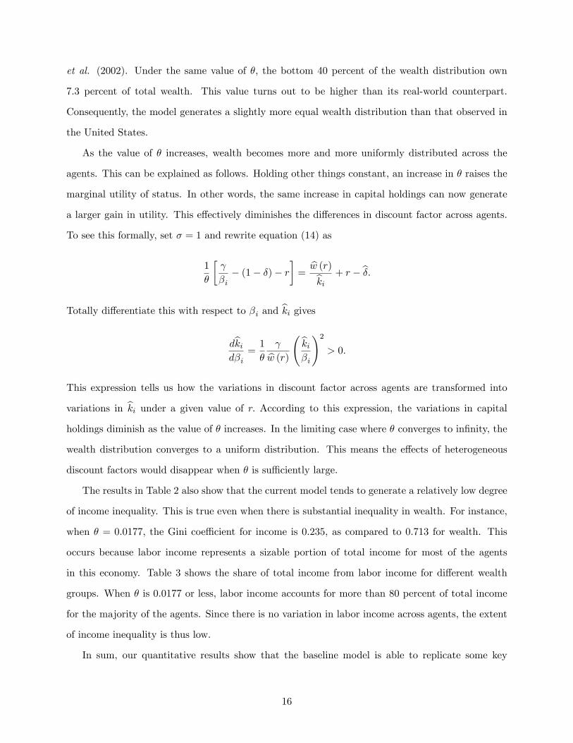
3 Endogenous Labor Supply

In this section, we extend the baseline model to include endogenous labor supply decisions. The

agent�s period utility function is now given by

u (c; s; l) =c1��

1� � + �s1��

1� � � �l1+1=�

1 + 1=�;

where l denote the amount of time spent on working, � is a positive parameter and � > 0 is the

intertemporal elasticity of substitution (IES) of labor. The agents�labor income is now endogenously

determined by their choice of working hours. The rest of the model is the same as in Section 2.

A balanced-growth equilibrium for this economy can be de�ned similarly as in Section 2.4. This

type of equilibrium now includes, among other things, a stationary distribution of labor which is

represent by l = (l1; l2;:::; lN ) : Let bkd (r) and bw (r) be the functions de�ned in (7) and (8). Theequilibrium values of

nbci;bki; lioNi=1

and the equilibrium rental rate r� are determined by

1

�

� �

�i� (1� �)� r

�=

�bcibki��

; (16)

bw (r)bci = � (li)1� ; (17)

bci = bw (r) li + �r � b��bki; (18)

NXi=1

bki = NXi=1

li

!bkd (r) ; (19)

where b� � � 1 + �: Equation (16) is the Euler equation for consumption evaluated along a

balanced-growth path. Equation (17) is the �rst-order condition with respect to labor. Equation

(18) is derived from the agent�s budget constraint. Equation (19) is the capital market equilibrium

condition.

We now consider the same numerical exercise as in Section 2.6. The production function again

takes the Cobb-Douglas form and the parameter values in Table 1 are used. The intertemporal

elasticity of substitution of labor is set to 0.4.10 To check the robustness of our �ndings, we also

consider two other values of this elasticity, which are 0.2 and 1.0. As in Section 2.6, we focus on the

10The same value is used in Chang and Kim (2006, 2007) among others.

18

relationship between � and the degree of inequality in wealth and income. We consider the same

set of values for � as in Table 2. In each case, the preference parameter � is chosen so that the

average amount of time spent on working is one-third and the depreciation rate � is chosen so that

the capital-output ratio is 3.0.

Table 5 shows the inequality measures obtained under � = 0:4: When comparing these to the

baseline results in Table 2, it is immediate to see that the two sets of results are almost identical.

Introducing endogenous labor supply decisions does not change the fundamental mechanism in the

baseline model. In particular, the model continues to generate a high degree of wealth inequality

when � is small and a relatively low degree of income inequality in general. Our numerical results

show that allowing for endogenous labor supply actually lowers the Gini coe¢ cient for income.

This can be explained by Figure 2, which shows the relationship between discount factor and labor

supply. Most of the agents in this economy, except those who are very patient, choose to have the

same amount of labor. Consequently, the distribution of labor is close to uniform with a long left

tail.11 This explains why the extended model generates a similar degree of income inequality as the

baseline model. Since labor supply decreases as the discount factor increases, an impatient agent

has less capital income but more labor income than a (very) patient agent. In other words, the two

sources of income are negatively correlated. This negative correlation in e¤ect reduces the degree

of income inequality in the extended model.

Finally, Table 6 shows that the results in Table 5 are robust to changes in the intertemporal elas-

ticity of substitution of labor. Speci�cally, increasing the elasticity from 0.2 to 1.0 only marginally

a¤ects the Gini coe¢ cients for wealth and income.

4 Human Capital Formation

4.1 The Model

In this section, we extend the baseline model to include human capital formation. The agents�

period utility function is now given by

u (c; s) = log c+ � log s; � > 0:

11 In all of our examples, the Gini coe¢ cient and the coe¢ cient of variaion for labor (and hence labor income) areclose to zero. These results are not reported in the paper but are available from the author upon request.

19

In each period, all agents are endowed with one unit of time which they can divide between market

work and on-the-job training. Denote by hit the stock of human capital of agent i at time t: If

this agent chooses to spend a fraction lit 2 [0; 1] of time on market work at time t; then his human

capital at time t+ 1 is given by

hit+1 = � (1� lit)� h�it + (1� �h)hit; (20)

where � > 0; � 2 (0; 1) ; � 2 (0; 1) ; and �h 2 (0; 1) is the depreciation rate of human capital. The

agent�s labor income at time t is given by wtlithit: We refer to lithit as the e¤ective unit of labor

and wt as the market wage rate for e¤ective unit of labor.

Let rt be the rental rate of physical capital at time t: Agent i�s problem is now given by

maxfcit;lit;kit+1;hit+1g1t=0

1Xt=0

�tiu (cit;sit)

subject to

cit + kit+1 � (1� �k) kit = wtlithit + rtkit;

kit+1 � 0; lit 2 [0; 1] ;

sit = kit;

the human capital accumulation equation in (20), and the initial conditions: ki0 > 0 and hi0 > 0:

The parameter �k 2 (0; 1) is the depreciation rate of physical capital. The rest of the model economy

is the same as in Section 2. In particular, long-term growth in per-capita variables is again fueled

by an exogenous improvement in labor-augmenting technology.12 The exogenous growth factor is

again given by � 1:

A balanced-growth equilibrium for this economy can be de�ned similarly as in Section 2.4. In

here we only present the key equations that characterize this type of equilibrium. A formal de�nition

can be found in Appendix B. A balanced-growth equilibrium now includes, among other things, a

stationary distribution of labor, l = (l1; l2; :::; lN ) ; and a stationary distribution of human capital,

12Unlike the endogenous growth model considered in Lucas (1988), human capital accumulation does not serve asthe engine of growth in here. This is implicitly implied by the condition � < 1: The main idea of introducing humancapital in this model is to increase the variation in labor income across agents.

20

h = (h1; h2; :::; hN ) : The equilibrium values ofnbci;bki; li; hioN

i=1and the equilibrium rental rate r�

are determined by

�i� (1� �k)� r = �

�bcibki�; (21)

bci = bw (r) lihi + �r � b��bki; (22)

li1� li

=1

�

�1

�h

�1

�i� (1� �h)

�� �

�; (23)

hi =

��

�h(1� li)�

� 11��

; (24)

andNXi=1

bki = NXi=1

lihi

!bkd (r) ; (25)

where b� � � 1+ �k: Equations (21) and (22) are derived from the Euler equation for consumption

and the agent�s budget constraint. Equations (23) and (24) are derived from the �rst-order condi-

tions with respect to lit and hit+1; and the human capital accumulation equation. Equation (19) is

the capital market equilibrium condition. The mathematical derivations of these can be found in

Appendix B.

According to (23) and (24), the distributions of labor and human capital are completely deter-

mined by two factors: (i) the distribution of subjective discount factor and (ii) the parameters in

the human capital accumulation process. In particular, these two distributions are independent of

the period utility function u (c; s), and thus the demand for status. If social status is not valued,

i.e., us (c; s) � 0; then the distribution of capital is degenerate but the distributions of labor and

human capital are non-degenerate.

4.2 Calibration

Parameters

In the quantitative exercise, we use the same speci�cation for production technology, and the same

distribution of discount factor as before. Speci�cally, the production function for goods takes the

Cobb-Douglas form with � = 0:33: The population contains 1,000 agents with subjective discount

factors uniformly distributed between 0.966 and 0.992. As for the parameter values in the human

21

capital production function, we normalize � to unity and set the values of � and � according to the

estimates reported in Heckman, et al. (1998). Using data from the National Longitudinal Survey

of Youth for the period 1979-1993, these authors �nd that the values of � and � for high school

graduates are 0.945 and 0.832, respectively. The corresponding values for college graduates are

0.939 and 0.871, respectively. The results generated by these two sets of values turn out to be

almost identical. In the following section, we only report the results for � = 0:939 and � = 0:871:13

As for the depreciation rate of human capital, Heckman, et al. (1998) assume that it is zero. Other

studies in the existing literature �nd that this rate is usually small and close to zero.14 We use a

depreciation rate of 3 percent, which is consistent with the estimates reported in Haley (1976).

It is now clear that the choice of � is key to explaining wealth inequality. In here we choose the

value of � so as to match the Gini coe¢ cient for wealth as reported in Rodríguez, et al. (2002).

Speci�cally, we target a value of 0.803 for the Gini coe¢ cient of wealth. The required value of �

is 0.0139. As explained above, the distributions of labor and human capital are independent of �:

Thus the distribution of earnings reported below is not in�uenced by this parameter. Finally, the

depreciation rate of physical capital is chosen so that the capital-output ratio is 3.0. The parameter

values used in the quantitative exercise are summarized in Table 7.

Findings

Table 8 summarizes the characteristics of the earnings, income and wealth distributions generated

by the model. The �rst three columns of the table show the Gini coe¢ cients, the coe¢ cients

of variation and the mean-to-median ratios for the three variables. The mean-to-median ratio is

intended to measure the degree of skewness in these distributions. The rest of Table 8 shows the

share of earnings, income and wealth held by agents in di¤erent percentiles of the corresponding

distribution.13The results for � = 0:945 and � = 0:832 are available from the author upon request.14See Browning, et al. (1999) Table 2.3 for a summary of this literature.

22

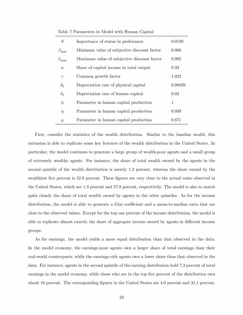
Table 7 Parameters in Model with Human Capital

� Importance of status in preferences 0.0139

�min Minimum value of subjective discount factor 0.966

�max Maximum value of subjective discount factor 0.992

� Share of capital income in total output 0.33

Common growth factor 1.022

�k Depreciation rate of physical capital 0.08029

�h Depreciation rate of human capital 0.03

� Parameter in human capital production 1

� Parameter in human capital production 0.939

� Parameter in human capital production 0.871

First, consider the statistics of the wealth distribution. Similar to the baseline model, this

extension is able to replicate some key features of the wealth distribution in the United States. In

particular, the model continues to generate a large group of wealth-poor agents and a small group

of extremely wealthy agents. For instance, the share of total wealth owned by the agents in the

second quintile of the wealth distribution is merely 1.2 percent, whereas the share owned by the

wealthiest �ve percent is 52.9 percent. These �gures are very close to the actual value observed in

the United States, which are 1.3 percent and 57.8 percent, respectively. The model is also to match

quite closely the share of total wealth owned by agents in the other quintiles. As for the income

distribution, the model is able to generate a Gini coe¢ cient and a mean-to-median ratio that are

close to the observed values. Except for the top one percent of the income distribution, the model is

able to replicate almost exactly the share of aggregate income owned by agents in di¤erent income

groups.

As for earnings, the model yields a more equal distribution than that observed in the data.

In the model economy, the earnings-poor agents own a larger share of total earnings than their

real-world counterparts, while the earnings-rich agents own a lower share than that observed in the

data. For instance, agents in the second quintile of the earning distribution hold 7.3 percent of total

earnings in the model economy, while those who are in the top �ve percent of the distribution own

about 16 percent. The corresponding �gures in the United States are 4.0 percent and 31.1 percent,

23

respectively. This result is not surprising because the data take into account retirees who have zero

earnings and the model does not. According to Rodríguez, et al. (2002), 22.5 percent of households

in their sample have zero earnings and a large portion of these are retired people. If we consider

only households headed by employed worker, then the Gini coe¢ cients for earnings in the United

States is 0.435. This value is very close to the one predicted by the model.

5 Summary and Conclusions

This paper presents a tractable dynamic competitive equilibrium model that can account for the

observed patterns of wealth and income inequality in the United States. In our baseline model,

consumers have di¤erent subjective discount factors and concern about their wealth-induced status

in the economy. The demand for status prevents the wealth distribution from collapsing into a

degenerate distribution. This allows the current study to explore the implications of heterogeneous

time preferences on wealth and income inequality. The rest of the model is identical to the standard

neoclassical growth model. A calibrated version of the baseline model is able to replicate some key

features of the wealth distribution in the United States. In particular, it is able to generate a large

group of wealth-poor consumers and a very small group of extremely wealthy ones. However, the

baseline model falls short in explaining income inequality. This problem remains even if we allow for

endogenous labor supply. To overcome this problem, we extend the baseline model by introducing

human capital formation. A calibrated version of this extended model successfully replicates the

distributions of wealth and income in the United States.

24

0.0

0.2

0.4

0.6

0.8

1.0

0.0 0.1 0.2 0.3 0.4 0.5 0.6 0.7 0.8 0.9 1.0

Share of Population

Shar

e of

 Wea

lth

Theta  =0.5

Theta  =0.05

Theta  =0.015

Theta  =0.005

Figure 1 Lorenz Curves for the Wealth Distribution.

25

0

0.1

0.2

0.3

0.4

0.966 0.971 0.976 0.982 0.987

S ubjec tiv e Dis c ount F ac tor

La

bo

r S

up

ply

theta =  0.0177

theta =  0.05

Figure 2: Relationship between Labor Supply and Subjective Discount Factor.

26

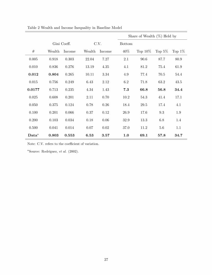
Table 2 Wealth and Income Inequality in Baseline Model

Share of Wealth (%) Held by

Gini Coe¤. C.V. Bottom

� Wealth Income Wealth Income 40% Top 10% Top 5% Top 1%

0.005 0.918 0.303 22.04 7.27 2.1 90.6 87.7 80.9

0.010 0.836 0.276 13.19 4.35 4.1 81.2 75.4 61.9

0.012 0.804 0.265 10.11 3.34 4.9 77.4 70.5 54.4

0.015 0.756 0.249 6.43 2.12 6.2 71.8 63.2 43.5

0.0177 0.713 0.235 4.34 1.43 7.3 66.8 56.8 34.4

0.025 0.608 0.201 2.11 0.70 10.2 54.3 41.4 17.1

0.050 0.375 0.124 0.78 0.26 18.4 29.5 17.4 4.1

0.100 0.201 0.066 0.37 0.12 26.9 17.6 9.3 1.9

0.200 0.103 0.034 0.18 0.06 32.9 13.3 6.8 1.4

0.500 0.041 0.014 0.07 0.02 37.0 11.2 5.6 1.1

Data� 0.803 0.553 6.53 3.57 1.0 69.1 57.8 34.7

Note: C.V. refers to the coe¢ cient of variation.

�Source: Rodríguez, et al. (2002).

27

Table 3 Share of Total Income from Labor Income (%) in Each Wealth Group

Percentiles in Wealth Distribution

� Bottom 1% 1-5% 5-10% 40-60% 90-95% 95-99% Top 1%

0.005 98.0 98.0 97.9 96.1 78.1 56.8 17.2

0.010 96.2 96.1 95.9 92.5 64.2 40.6 10.0

0.012 95.4 95.3 95.1 91.1 60.0 36.5 8.7

0.015 94.4 94.2 94.0 89.1 54.7 32.0 7.7

0.0177 93.4 93.3 92.9 87.4 50.9 29.2 7.6

0.025 91.0 90.8 90.4 83.3 44.6 26.6 11.1

0.050 84.6 84.3 83.7 74.6 45.6 38.1 33.1

0.100 78.0 77.7 77.1 69.4 54.9 52.5 51.1

0.200 73.2 72.9 72.5 67.6 61.0 60.1 59.6

0.500 69.6 69.5 69.3 67.1 64.6 64.4 64.2

Data� 98.9 95.9 98.1 94.0 69.8 52.3 33.6

*Source: Rodríguez, et al. (2002) Table 7, excluding transfers.

28

Table 4 Wealth Inequality under Di¤erent Ranges of Discount Factor

Share of Wealth (%) Held by

Bottom

� �min �max Gini C.V. 40% Top 10% Top 5% Top 1%

0.0177 0.966 0.992 0.713 4.34 7.3 66.8 56.8 34.4

0.956 0.982 0.719 4.55 7.1 67.5 57.7 35.6

0.946 0.972 0.724 4.78 7.0 68.1 58.5 36.7

0.979 0.992 0.486 1.21 14.1 40.4 26.7 7.6

0.966 0.979 0.494 1.26 13.8 41.4 27.7 8.1

0.953 0.992 0.809 10.43 4.8 77.9 71.1 55.3

0.050 0.966 0.992 0.375 0.78 18.4 29.5 17.4 4.1

0.956 0.982 0.381 0.80 18.1 30.1 17.8 4.2

0.946 0.972 0.388 0.82 17.8 30.6 18.2 4.4

0.979 0.992 0.199 0.36 27.0 17.6 9.2 1.9

0.966 0.979 0.204 0.37 26.7 17.8 9.4 2.0

0.953 0.992 0.512 1.34 13.2 43.2 29.3 8.9

0.100 0.966 0.992 0.201 0.37 26.9 17.6 9.3 1.9

0.956 0.982 0.205 0.37 26.7 17.8 9.4 2.0

0.946 0.972 0.209 0.38 26.4 18.1 9.5 2.0

0.979 0.992 0.102 0.18 32.9 13.2 6.8 1.4

0.966 0.979 0.104 0.18 32.8 13.3 6.8 1.4

0.953 0.992 0.295 0.57 21.9 23.3 12.9 2.8

Note: C.V. refers to the coe¢ cient of variation. Figures in bold are the benchmark results as shown in

Table 2.

29

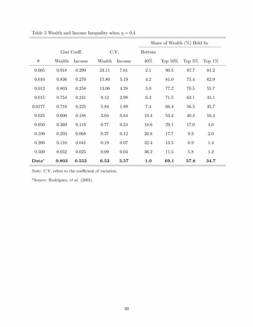
Table 5 Wealth and Income Inequality when � = 0:4

Share of Wealth (%) Held by

Gini Coe¤. C.V. Bottom

� Wealth Income Wealth Income 40% Top 10% Top 5% Top 1%

0.005 0.918 0.299 23.11 7.61 2.1 90.5 87.7 81.2

0.010 0.836 0.270 15.80 5.19 4.2 81.0 75.4 62.9

0.012 0.803 0.258 13.06 4.28 5.0 77.2 70.5 55.7

0.015 0.754 0.241 9.12 2.98 6.3 71.5 63.1 45.1

0.0177 0.710 0.225 5.84 1.89 7.4 66.4 56.5 35.7

0.025 0.600 0.188 2.04 0.64 10.4 53.4 40.4 16.4

0.050 0.369 0.118 0.77 0.24 18.6 29.1 17.0 4.0

0.100 0.203 0.068 0.37 0.12 26.8 17.7 9.3 2.0

0.200 0.110 0.041 0.19 0.07 32.4 13.5 6.9 1.4

0.500 0.052 0.025 0.09 0.04 36.2 11.5 5.8 1.2

Data� 0.803 0.553 6.53 3.57 1.0 69.1 57.8 34.7

Note: C.V. refers to the coe¢ cient of variation.

�Source: Rodríguez, et al. (2002).

30

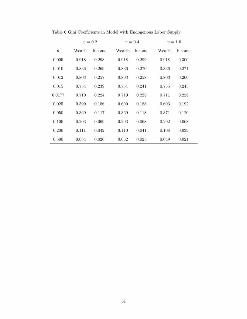
Table 6 Gini Coe¢ cients in Model with Endogenous Labor Supply

� = 0:2 � = 0:4 � = 1:0

� Wealth Income Wealth Income Wealth Income

0.005 0.918 0.298 0.918 0.299 0.918 0.300

0.010 0.836 0.269 0.836 0.270 0.836 0.271

0.012 0.803 0.257 0.803 0.258 0.803 0.260

0.015 0.754 0.239 0.754 0.241 0.755 0.243

0.0177 0.710 0.224 0.710 0.225 0.711 0.228

0.025 0.599 0.186 0.600 0.188 0.603 0.192

0.050 0.369 0.117 0.369 0.118 0.371 0.120

0.100 0.203 0.069 0.203 0.068 0.202 0.068

0.200 0.111 0.042 0.110 0.041 0.108 0.039

0.500 0.054 0.026 0.052 0.025 0.049 0.021

31

Table8MainResultsinModelwithHumanCapital

Share(%)HeldbyAgentsinEachGroup

Mean-to-

Bottom

Quintiles

Top

Top

Top

Gini

C.V.

Median

1%1-5%

5-10%

1st

2nd

3rd

4th

5th

10%

5%1%

Earnings

Model

0.458

0.86

1.52

0.1

0.7

0.9

4.1

7.3

13.4

25.4

49.2

29.1

15.9

3.7

Data

0.611

2.65

1.57

-0.2

0.0

0.0

-0.2

4.0

13.0

22.9

60.2

42.9

31.1

15.3

Income

Model

0.572

1.34

2.04

0.1

0.5

0.7

2.9

5.3

10.0

20.3

60.4

42.7

28.3

9.3

Data

0.553

3.57

1.61

-0.1

0.1

0.5

2.4

7.2

12.5

20.0

58.0

43.1

32.8

17.5

Wealth

Model

0.803

2.61

6.90

0.0

0.0

0.1

0.5

1.2

3.0

9.8

82.9

70.3

52.9

19.2

Data

0.803

6.53

4.03

-0.2

-0.1

0.0

-0.3

1.3

5.0

12.2

81.7

69.1

57.8

34.7

Datasource:Rodríguez,etal.(2002).

32

Appendix A

Proof of Theorem 1

The proof of this theorem is divided into three main steps. First, it is shown that there exists a

rental price er1 > b� such that bks (r) ! 1 as r approaches er1 from the left. Since both bks (r) andbkd (r) are continuous on �b�; er1� and bks (er1) <1; this result, together with bkd �b�� > bks �b��, wouldensure the existence of at least one value of r 2

�b�; er1� that solves the equationbkd (r) = bks (r) : (26)

The second step is to show that there exists at most one solution on the interval (0; er1) : Together,these two steps show that a unique r� exists in the interval

�b�; er1� : Finally, it is shown that �i > �j

implies bci > bcj and bki > bkj :Step 1 For each i 2 f1; 2; :::; Ng ; one can show that there exists a unique value eri > b� that solves

�

�i� (1� �)� r = h

�r � b�� :

First, h (0) = 0 < �

�i� (1� �) : Second, the left-hand side of the above expression is strictly

decreasing in r, while the right-hand side is strictly increasing in r. Hence the two cross at most

once. It is straightforward to show that eri < bri � �=�i � (1� �) and erN � erN�1 � : : : � er1 > b�given the ordering 1 > �1 � �2 � : : : � �N > 0:

By the de�nitions of g1 (r) and er1; it must be the case that g1 (r)!1 as r approaches er1 fromthe left. Since er1 � eri < bri for any i � 2; we have gi (r) > 0 for all i � 2 when r is arbitrarily closeto er1: Thus, as r approaches er1 from the left, we have

bks (r) = 1

N

NXi=1

gi (r)!1:

33

Step 2 To establish the uniqueness of r�; we need to consider the derivative of bks (r) : Usingequation (11), one can derive the derivative of gi (r), which is given by

g0i (r) =1bw (r)

([gi (r)]

2 + bw0 (r) gi (r) + [gi (r)]2

h0 (zi (r))

);

where zi (r) � bw (r) =gi (r) + r � b� and bw0 (r) = �bkd (r) < 0: Hence the derivative of bks (r) is givenby

d

drbks (r) =

1

N

NXi=1

g0i (r)

=1bw (r)

(1

N

NXi=1

[gi (r)]2 � bkd (r)bks (r) + 1

N

NXi=1

[gi (r)]2

h0 (zi (r))

):

Let r� be any solution of (26). The derivative of bks (r) at r = r� is

1bw (r�)(1

N

NXi=1

[gi (r�)]2 �

hbks (r�)i2 + 1

N

NXi=1

[gi (r�)]2

h0 (zi (r�))

);

after we imposed the condition bkd (r�) = bks (r�) : The above expression is strictly positive as1

N

NXi=1

[gi (r�)]2 �

"1

N

NXi=1

gi (r�)

#2=hbks (r�)i2 ;

and h0 (z) > 0: Since bkd (r) is monotonically decreasing, this means bks (r) must be cutting bkd (r)from below at every intersection point. Since both bkd (r) and bks (r) are continuous, if there existsmore than one solution of (26) then at least of them must have bks (r) cutting bkd (r) from above.

This gives rise to a contradiction and hence establishes the uniqueness of r�:

Step 3 Totally di¤erentiate the equation

�

�� (1� �)� r = h

� bw (r)bk + r � b��

34

with respect to � and bk yieldsdbkd�

= �

bk�

!2 �h0� bw (r)bk + r � b����1 > 0:

Hence �i > �j implies bki > bkj : Since the equilibrium rental rate r� is strictly greater than b�; bci ispositively related to bki according to (9).

This completes the proof of Theorem 1.

35

Appendix B

This section provides the technical details of the model in Section 4. First, we de�ne a balanced-

growth equilibrium for this economy. A competitive equilibrium consists of sequences of distri-

butions of individual variables, fct;kt; lt;htg1t=0 ; sequences of aggregate inputs, fKt; Ltg1t=0 ; and

sequences of prices, fwt; rtg1t=0 ; so that

(i) Given the prices fwt; rtg1t=0 ; the sequences fcit; kit; lit; hitg1t=0 solve agent i�s problem.

(ii) In each period t � 0; given the prices wt and rt; the aggregate inputs Kt and Lt solve the

representative �rm�s problem.

(iii) All markets clear in every period, so that for each t � 0;

Kt =

NXi=1

kit and Lt =

NXi=1

lithit:

A set of sequences S = fct;kt; lt;ht;Kt; Lt; wt; rtg1t=0 is called a balanced-growth equilibrium if

the following conditions are satis�ed:

(i) S is a competitive equilibrium as de�ned above.

(ii) The rental rate of capital is stationary over time, i.e., rt = r� for all t:

(iii) The distributions of labor and human capital are stationary over time.

(iv) Individual consumption and capital, aggregate capital and the wage rate are all growing at

the same constant rate. In particular, the common growth factor is � 1:

We now provide the mathematical derivations of equations (21)-(24). Let �it and it be the

multipliers for the budget constraint and the human capital accumulation equation, respectively.

The �rst-order conditions for the agent�s problem are given by

uc (cit; kit) = �it; (27)

�itwthit = it�� (1� lit)��1 h�it; (28)

36

�it = �i [us (cit+1; kit+1) + �it+1 (1 + rt+1 � �k)] ; (29)

it = �i

n�it+1wt+1lit+1 + it+1

h�� (1� lit+1)� h��1it+1 + (1� �h)

io: (30)

Combining (27) and (29) gives

uc (cit; kit)

uc (cit+1; kit+1)= �i

�us (cit+1; kit+1)

uc (cit+1; kit+1)+ 1 + rt+1 � �k

�:

Equation (21) can be obtained from this after imposing the balanced-growth conditions: cit =

tbci and kit = tbki: The derivation of (22) is straightforward and is omitted. Along a balanced-growth equilibrium path, individual human capital is stationary. It follows from the human capital

accumulation equation that

�hhi = � (1� li)� h�i :

Equation (24) follows immediately from this expression. Finally, combining (28) and (30) gives

it = �i it+1

n� (1� lit+1)��1 h��1it+1 [� (1� lit+1) + �lit+1] + (1� �h)

o:

In the balanced-growth equilibrium, the multiplier it is stationary over time. To see this, combine

(27) and (28) to getwtcit= it�� (1� lit)��1 h

��1it :

In a balanced-growth equilibrium, lit and hit are stationary while wt and cit are growing at the same

rate. Thus it must be stationary over time. Thus, in this kind of equilibrium, we have

1 = �i

n� (1� li)��1 h��1i [� (1� li) + �li] + (1� �h)

o:

Equation (23) can be obtained by substituting (24) into this.

37

References

[1] Aiyagari, S.R., �Uninsured Idiosyncratic Risk and Aggregate Saving,�Quarterly Journal of

Economics 109 (1994), 659-684.

[2] Bakshi, G.S. and Z. Chen, �The Spirit of Capitalism and Stock-Market Prices,� American

Economic Review 86 (1996), 133-157.

[3] Becker, R.A., �On the Long-Run Steady State in a Simple Dynamic Model of Equilibrium with

Heterogeneous Households,�Quarterly Journal of Economics 95 (1980), 375-382.

[4] Boileau, M. and R. Braeu, �The Spirit of Capitalism, Asset Returns, and the Business Cycle,�

Macroeconomic Dynamics 11 (2007), 214-230.

[5] Boyd, J.H. III, �Recursive Utility and the Ramsey Problem,�Journal of Economic Theory 50

(1990), 326-345.

[6] Browning, M., L.P. Hansen, and J.J. Heckman, �Micro Data and General Equilibrium Models,�

in J.B. Taylor and M. Woodford, eds., Handbook of Macroeconomics, Volume 1, (North Holland

Press, 1999), 543-633.

[7] Castañeda, A., J. Díaz-Giménez, and J. Ríos-Rull, �Accounting for the U.S. Earnings and

Wealth Inequality,�Journal of Political Economy 111 (2003), 818-857.

[8] Chang, Y. and S. Kim, �From Individual to Aggregate Labor Supply: A Quantitative Analysis

Based on a Heterogeneous Agent Macroeconomy,� International Economic Review 47 (2006),

1-27.

[9] Chang, Y. and S. Kim, �Heterogeneity and Aggregation: Implications for Labor-Market Fluc-

tuations,�American Economic Review 97 (2007), 1939-1956.

[10] Chang, W. and H. Tsai, �Money, Social Status, and Capital Accumulation in a Cash-in-

Advance Model: Comment,�Journal of Money, Credit and Banking 33 (2003), 657-661.

[11] Chen, H.J. and J.T. Guo, �Social Status and the Growth E¤ect of Money,�Japanese Economic

Review 60 (2009), 133-141.

38

[12] Cole, H.L., G.J. Mailath and A. Postlewaite, �Social Norms, Savings Behavior, and Growth,�

Journal of Political Economy 100 (1992), 1092-1125.

[13] Espino, E., �On Ramsey�s Conjecture: E¢ cient Allocations in the Neoclassical Growth Model

with Private Information,�Journal of Economic Theory 121 (2005), 192-213.

[14] Frederick, S., G. Loewenstein, T. O�Donoghue, �Time Discounting and Time Preferences: A

Critical Review,�Journal of Economic Literature 40 (2002), 351-401.

[15] Gong, L. and H. Zou, �Money, Social Status, and Capital Accumulation in a Cash-in-Advance

Model,�Journal of Money, Credit and Banking 33 (2001), 284-293.

[16] Haley, W.J., �Estimation of the Earnings Pro�le from Optimal Human Capital Accumulation,�

Econometrica 44 (1976), 1223-1238.

[17] Hausman, J.A., �Individual Discount Rates and the Purchase and Utilization of Energy-Using

Durables,�Bell Journal of Economics 10 (1979), 33-54.

[18] Heckman, J.J., L. Lochner, and C. Taber, �Explaining Rising Wage Inequality: Explorations

with a Dynamic General Equilibrium Model for Labor Earnings with Heterogeneous Agents,�

Review of Economic Dynamics 1 (1998), 1-58.

[19] Huggett, M., �The Risk-Free Rate in Heterogeneous-Agent Incomplete-Insurance Economies,�

Journal of Economic Dynamics and Control 17 (1993), 953-969.

[20] Krusell, P. and A.A. Smith, �Income and Wealth Heterogeneity in the Macroeconomy,�Journal

of Political Economy 106 (1998), 867-896.

[21] Kurz, M., �Optimal Economic Growth and Wealth E¤ects,�International Economic Review 9

(1968), 348-357.

[22] Lawrance, E.C., �Poverty and the Rate of Time Preference: Evidence from Panel Data,�

Journal of Political Economy 99 (1991), 54-77.

[23] Lucas, R.E., �On the Mechanics of Economic Development,�Journal of Monetary Economics

22 (1998), 3-42.

39

[24] Lucas, R.E. and N.L. Stokey, �Optimal Growth with Many Consumers,�Journal of Economic

Theory 32 (1984), 139-171.

[25] Luo, Y. and E.R. Young, �The Wealth Distribution and the Demand for Status,�Macroeco-

nomic Dynamics 13 (2009), 1-30.

[26] Quadrini, V. and J. Ríos-Rull, �Understanding the U.S. Distribution of Wealth,�Federal Re-

serve Bank of Minneapolis Quarterly Review 21 (1997), 22-36.

[27] Ramsey, F.P., �A Mathematical Theory of Saving,�Economic Journal 38 (1929), 543-559.

[28] Rodriguez, S.B., J. Díaz-Giménez, V. Quadrini, and J. Ríos-Rull, �Updated Facts on the

U.S. Distributions of Earnings, Income, and Wealth,� Federal Reserve Bank of Minneapolis

Quarterly Review 26 (2002), 2-35.

[29] Samwick, A.A., �Discount Rate Heterogeneity and Social Security Reform,�Journal of Devel-

opment Economics 57 (1998), 117-146.

[30] Sarte, P.G., �Progressive Taxation and Income Inequality in Dynamic Competitive Equilib-

rium,�Journal of Public Economics 66 (1997), 145-171.

[31] Smith, W.T., �Risk, the Spirit of Capitalism and Growth: The Implications of a Preference

for Capital,�Journal of Macroeconomics 21 (1999), 241-262.

[32] Sorger, G., �On the Long-Run Distribution of Capital in the Ramsey Model,� Journal of

Economic Theory 105 (2002), 226-243.

[33] Sorger, G., �Strategic Saving Decisions in the In�nite-Horizon Model,�Economic Theory 36

(2008), 353-377.

[34] Warner, J.T. and S. Pleeter, �The Personal Discount Rate: Evidence from Military Downsizing

Programs,�American Economic Review 91 (2001), 33-53.

[35] Zou, H., ��The Spirit of Capitalism�and Long-Run Growth,� European Journal of Political

Economy 10 (1994), 279-293.

40