Embed Size (px)
Citation preview

Time series, connectivity and networks
Dimitris Kugiumtzis
Department of Electrical and Computer Engineering,Aristotle University of Thessaloniki
Thessaloniki 54124, Greecee-mail: [email protected] http:\\users.auth.gr\dkugiu
7 November 2013
Multivariate time series =⇒ connectivity =⇒ networks
Dimitris Kugiumtzis Time series, connectivity and networks
Outline
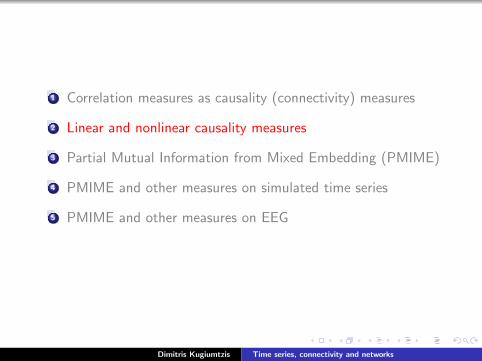
1 Correlation measures as causality (connectivity) measures
2 Linear and nonlinear causality measures
3 Partial Mutual Information from Mixed Embedding (PMIME)
4 PMIME and other measures on simulated time series
5 PMIME and other measures on EEG
Dimitris Kugiumtzis Time series, connectivity and networks

Financial World Markets
correlation?
�causality
?
-
-
�������
6
?Does USA drive theother markets?
Dimitris Kugiumtzis Time series, connectivity and networks

Electroencephalogram (EEG)
http://en.wikipedia.org/wiki/File:EEG cap.jpg
Dimitris Kugiumtzis Time series, connectivity and networks
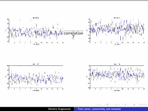
correlation?
Dimitris Kugiumtzis Time series, connectivity and networks

-�causality
?
Dimitris Kugiumtzis Time series, connectivity and networks
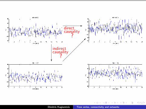
-directcausality
?
? �������
indirectcausality
?
Dimitris Kugiumtzis Time series, connectivity and networks

-
�������
6
?Does C3 drivesother channels?
Dimitris Kugiumtzis Time series, connectivity and networks
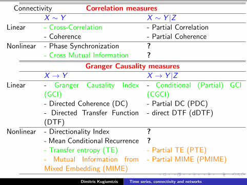
Connectivity Correlation measuresX ∼ Y X ∼ Y |Z
Linear - Cross-Correlation- Coherence
- Partial Correlation- Partial Coherence
Nonlinear - Phase Synchronization- Cross Mutual Information
??
Granger Causality measuresX → Y X → Y |Z
Linear - Granger Causality Index(GCI)- Directed Coherence (DC)- Directed Transfer Function(DTF)
- Conditional (Partial) GCI(CGCI)- Partial DC (PDC)- direct DTF (dDTF)
Nonlinear - Directionality Index- Mean Conditional Recurrence- Transfer entropy (TE)- Mutual Information fromMixed Embedding (MIME)
??- Partial TE (PTE)- Partial MIME (PMIME)
Dimitris Kugiumtzis Time series, connectivity and networks

1 Correlation measures as causality (connectivity) measures
2 Linear and nonlinear causality measures
3 Partial Mutual Information from Mixed Embedding (PMIME)
4 PMIME and other measures on simulated time series
5 PMIME and other measures on EEG
Dimitris Kugiumtzis Time series, connectivity and networks

Correlation measures
Bivariate time series {xt , yt}nt=1
Linear correlation measures:
Estimate of cross-covariance
cXY (τ) = γXY (τ) =1
n − τ
n−τ∑t=1
(xt − x)(yt+τ − y)
x and y are sample means.
Estimate of cross-correlation:
rXY (τ) = ρXY (τ) =cXY (τ)
cXY (0)=
cXY (τ)
sX sY
sX and sY are sample standard deviations.
|rXY (τ)| ≤ 1
rXY (τ) = rYX (−τ) but rXY (τ) 6= rXY (−τ)
Dimitris Kugiumtzis Time series, connectivity and networks

Noninear correlation measures:Entropy: information from each sample of X (assume properdiscretization of X )
H(X ) =∑x
pX (x) log pX (x)
Mutual information: information for Y knowing X and vice versa
I (X ,Y ) = H(X )+H(Y )−H(X ,Y ) =∑x ,y
pXY (x , y) logpXY (x , y)
pX (x)pY (y)
For X → Xt and Y → Yt+τ ,cross-delayed mutual information:
IXY (τ) = I (Xt ,Yt+τ ) =∑
xt ,yt+τ
pXtYt+τ (xt , yt+τ ) logpXtYt+τ (xt , yt+τ )
pXt (xt)pYt+τ (yt+τ )
To compute IXY (τ) make a partition of {xt}nt=1, a partition of{yt}nt=1 and compute probabilities for each cell from the relativefrequency.
Dimitris Kugiumtzis Time series, connectivity and networks

rXY (0) 6= 0:
=⇒ (linear) correlation of xt and yt
=⇒ systems X and Y are correlated, X ∼ Y
rXY (τ) 6= 0:
=⇒ (linear) correlation of xt and yt+τ
=⇒ X effects the future of Y
=⇒ X → Y
rXY (−τ) 6= 0 =⇒ Y → X
Thus rXY (τ) and IXY (τ) indicate the direction of interaction.
Can they also be used as causality measures?Not the most appropriate, but they can
Dimitris Kugiumtzis Time series, connectivity and networks
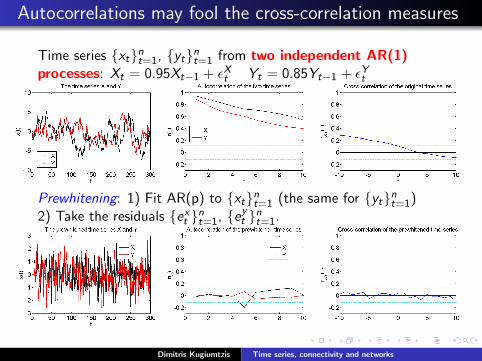
Autocorrelations may fool the cross-correlation measures
Time series {xt}nt=1, {yt}nt=1 from two independent AR(1)processes: Xt = 0.95Xt−1 + εXt Yt = 0.85Yt−1 + εYt
Prewhitening: 1) Fit AR(p) to {xt}nt=1 (the same for {yt}nt=1)2) Take the residuals {ext }nt=1, {eyt }nt=1.
Dimitris Kugiumtzis Time series, connectivity and networks
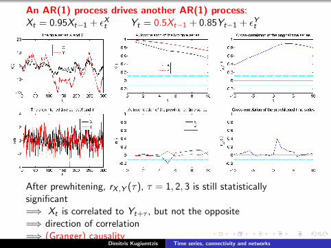
An AR(1) process drives another AR(1) process:Xt = 0.95Xt−1 + εXt Yt = 0.5Xt−1 + 0.85Yt−1 + εYt
After prewhitening, rX ,Y (τ), τ = 1, 2, 3 is still statisticallysignificant=⇒ Xt is correlated to Yt+τ , but not the opposite=⇒ direction of correlation=⇒ (Granger) causality
Dimitris Kugiumtzis Time series, connectivity and networks

Two inter-dependent AR(1) processes:Xt = 1.2Xt−1−0.5Yt−1 + εXt Yt = 0.6Xt−1 + 0.3Yt−1 + εYt
After prewhitening, the statistically significant cross-correlationsare for both positive and negative delays=⇒ Xt is correlated to Yt+|τ | and to Yt−|τ |,=⇒ interdependence
Dimitris Kugiumtzis Time series, connectivity and networks

Example: Returns for USA, UnitedKingdom, Greece and Australia.
returns:xt = log(yt)− log(yt−1)
X :AUS, Y :GRE
rXY (0) = 0.58
�rXY (−1) = 0.19
-rXY (1) = 0.02
Is the measure significant?Can I draw a link? (directed / undirected)
Dimitris Kugiumtzis Time series, connectivity and networks
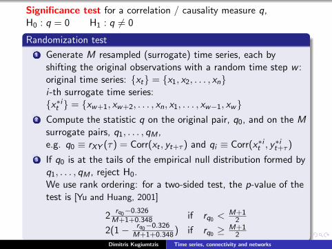
Significance test for a correlation / causality measure q,H0 : q = 0 H1 : q 6= 0
Randomization test
1 Generate M resampled (surrogate) time series, each byshifting the original observations with a random time step w :original time series: {xt} = {x1, x2, . . . , xn}i-th surrogate time series:{x∗it } = {xw+1, xw+2, . . . , xn, x1, . . . , xw−1, xw}
2 Compute the statistic q on the original pair, q0, and on the Msurrogate pairs, q1, . . . , qM ,e.g. q0 ≡ rXY (τ) = Corr(xt , yt+τ ) and qi ≡ Corr(x∗it , y
∗it+τ )
3 If q0 is at the tails of the empirical null distribution formed byq1, . . . , qM , reject H0.We use rank ordering: for a two-sided test, the p-value of thetest is [Yu and Huang, 2001]
2rq0−0.326
M+1+0.348 if rq0 <M+1
2
2(1− rq0−0.326M+1+0.348 ) if rq0 ≥ M+1
2
Dimitris Kugiumtzis Time series, connectivity and networks
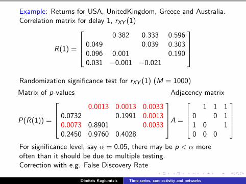
Example: Returns for USA, UnitedKingdom, Greece and Australia.Correlation matrix for delay 1, rXY (1)
R(1) =
0.382 0.333 0.596
0.049 0.039 0.3030.096 0.001 0.1900.031 −0.001 −0.021
Randomization significance test for rXY (1) (M = 1000)
Matrix of p-values
P(R(1)) =
0.0013 0.0013 0.0033
0.0732 0.1991 0.00130.0073 0.8901 0.00330.2450 0.9760 0.4028
Adjacency matrix
A =
1 1 1
0 0 11 0 10 0 0
For significance level, say α = 0.05, there may be p < α moreoften than it should be due to multiple testing.Correction with e.g. False Discovery Rate
Dimitris Kugiumtzis Time series, connectivity and networks
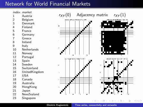
Network for World Financial Markets
index market1 Austria2 Belgium3 Denmark4 Finland5 France6 Germany7 Greece8 Ireland9 Italy10 Netherlands11 Norway12 Portugal13 Spain14 Sweden15 Switzerland16 UnitedKingdom17 USA18 Canada19 Australia20 HongKong21 Japan22 NewZealand23 Singapore
rXY (0) Adjacency matrix rXY (1)
IXY (0) Adjacency matrix IXY (1)
Dimitris Kugiumtzis Time series, connectivity and networks

Correlation network, nodes: 23 financial markets, directed links: rXY (1)
Dimitris Kugiumtzis Time series, connectivity and networks
1 Correlation measures as causality (connectivity) measures
2 Linear and nonlinear causality measures
3 Partial Mutual Information from Mixed Embedding (PMIME)
4 PMIME and other measures on simulated time series
5 PMIME and other measures on EEG
Dimitris Kugiumtzis Time series, connectivity and networks

Linear causality measures (direct and indirect)
Idea of Granger causality X → Y : [Brandt & Williams, 2007, Chp 2]
predict Y better when including X in the regression model.
Measure 1a: Granger Causality Index (GCI)
Bivariate time series {xt , yt}nt=1
driving system: X , response system: Y
Model 1 (restricted, R, X absent in the model):
yt =
p∑i=1
aiyt−i + eR,t
Model 2 (unrestricted, U, X present in the model):
yt =
p∑i=1
aiyt−i +
p∑i=1
bixt−i + eU,t
GCIX→Y = lnVar(eR,t)
Var(eU,t)GCIX→Y > 0⇒ X → Y holds
Dimitris Kugiumtzis Time series, connectivity and networks

Parametric significance test for GCI
GCIX→Y > 0 ?⇒ Significance test
If X does not Granger causes Y then the contribution of X -lags inthe unrestricted model should be insignificant ⇒
the terms of X should be insignificant
H0: bi = 0, for all i = 1, . . . , pH1: bi 6= 0, for any of i = 1, . . . , p
Snedecor-Fisher test (F-test):
F =(SSER − SSEU)/p
SSEU/ndf
SSE: sum of squared errors
ndf: number of degrees of freedoms, ndf = (n − p)− 2p,n − p: number of equations,2p: number of coefficients in the U-model.
Dimitris Kugiumtzis Time series, connectivity and networks

Linear causality measures (direct and indirect)
Measure 1b: Conditional Granger Causality Index (CGCI)
K time series {xt , yt}nt=1 and {zt}nt=1 = {z1,t , z2,t , . . . , zK−2,t}nt=1
driving system: X , response system: Y ,conditioning on system Z , Z = {Z1,Z2, . . . ,ZK−2}
Model 1 (restricted, R, X absent in the model):
yt =
p∑i=1
aiyt−i +
p∑i=1
Aizt−i + eR,t
Model 2 (unrestricted, U, X present in the model):
yt =
p∑i=1
aiyt−i +
p∑i=1
bixt−i +
p∑i=1
Aizt−i + eU,t
CGCIX→Y |Z = lnVar(eR,t)
Var(eU,t)
Dimitris Kugiumtzis Time series, connectivity and networks
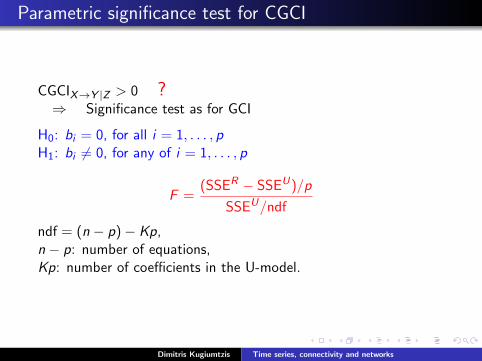
Parametric significance test for CGCI
CGCIX→Y |Z > 0 ?⇒ Significance test as for GCI
H0: bi = 0, for all i = 1, . . . , pH1: bi 6= 0, for any of i = 1, . . . , p
F =(SSER − SSEU)/p
SSEU/ndf
ndf = (n − p)− Kp,n − p: number of equations,Kp: number of coefficients in the U-model.
Dimitris Kugiumtzis Time series, connectivity and networks
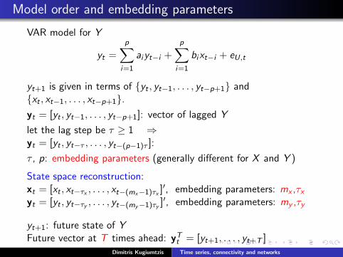
Model order and embedding parameters
VAR model for Y
yt =
p∑i=1
aiyt−i +
p∑i=1
bixt−i + eU,t
yt+1 is given in terms of {yt , yt−1, . . . , yt−p+1} and{xt , xt−1, . . . , xt−p+1}.yt = [yt , yt−1, . . . , yt−p+1]: vector of lagged Y
let the lag step be τ ≥ 1 ⇒yt = [yt , yt−τ , . . . , yt−(p−1)τ ]:
τ , p: embedding parameters (generally different for X and Y )
State space reconstruction:xt = [xt , xt−τx , . . . , xt−(mx−1)τx ]′, embedding parameters: mx ,τxyt = [yt , yt−τy , . . . , yt−(my−1)τy ]′, embedding parameters: my ,τy
yt+1: future state of YFuture vector at T times ahead: yTt = [yt+1, . . . , yt+T ]
Dimitris Kugiumtzis Time series, connectivity and networks

Nonlinear causality measures (direct and indirect)
xt = [xt , xt−τx , . . . , xt−(mx−1)τx ]′, embedding parameters: mx ,τxyt = [yt , yt−τy , . . . , yt−(my−1)τy ]′, embedding parameters: my ,τyFuture vector at T times ahead: yTt = [yt+1, . . . , yt+T ]
Mutual Information of X and Y :I (X ;Y ) = H(X ) + H(Y )− H(X ,Y )
Measure 2a: Transfer Entropy (TE) [Schreiber, 2000]
Measure the effect of X on Y at T times ahead, accounting(conditioning) for the effect from its own current state
TEX→Y = I (yTt ; xt |yt)= H(xt , yt)− H(yTt , xt , yt) + H(yTt , yt)− H(yt)
=∑
p(yt+T , xt , yt) logp(yt+T |xt , yt)p(yt+T |yt)
Joint entropies (and distributions) can have high dimension!
Dimitris Kugiumtzis Time series, connectivity and networks
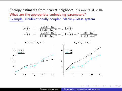
Entropy estimates from nearest neighbors [Kraskov et al, 2004]
What are the appropriate embedding parameters?Example: Unidirectionally coupled Mackey-Glass system
x(t) = 0.2x(t−∆x )1+x(t−∆x )10 − 0.1x(t)
y(t) =0.2y(t−∆y )
1+y(t−∆y )10 − 0.1y(t) + C x(t−∆x )1+x(t−∆x )10 .
Dimitris Kugiumtzis Time series, connectivity and networks
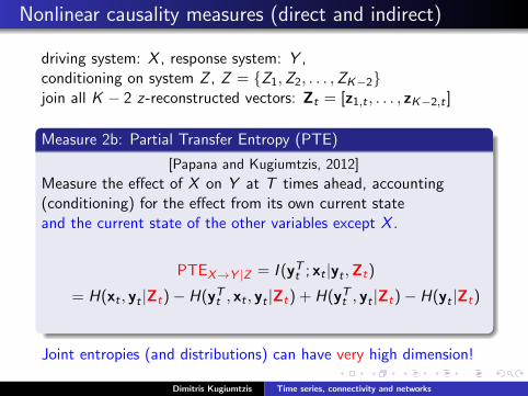
Nonlinear causality measures (direct and indirect)
driving system: X , response system: Y ,conditioning on system Z , Z = {Z1,Z2, . . . ,ZK−2}join all K − 2 z-reconstructed vectors: Zt = [z1,t , . . . , zK−2,t ]
Measure 2b: Partial Transfer Entropy (PTE)
[Papana and Kugiumtzis, 2012]
Measure the effect of X on Y at T times ahead, accounting(conditioning) for the effect from its own current stateand the current state of the other variables except X .
PTEX→Y |Z = I (yTt ; xt |yt ,Zt)
= H(xt , yt |Zt)− H(yTt , xt , yt |Zt) + H(yTt , yt |Zt)− H(yt |Zt)
Joint entropies (and distributions) can have very high dimension!
Dimitris Kugiumtzis Time series, connectivity and networks

1 Correlation measures as causality (connectivity) measures
2 Linear and nonlinear causality measures
3 Partial Mutual Information from Mixed Embedding (PMIME)
4 PMIME and other measures on simulated time series
5 PMIME and other measures on EEG
Dimitris Kugiumtzis Time series, connectivity and networks

Mutual Information from Mixed Embedding - 1
Bivariate time series {xt , yt}nt=1
driving system: X , response system: Y
The idea: [Vlachos & Kugiumtzis, 2010]
1 Find a mixed embedding of varying delays from X and Y thatexplains best the future of Y .
2 Quantify the information on Y ahead that is explained by theX -components of the mixed embedding vector.
Dimitris Kugiumtzis Time series, connectivity and networks
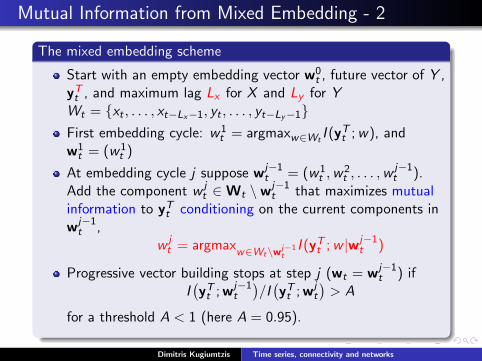
Mutual Information from Mixed Embedding - 2
The mixed embedding scheme
Start with an empty embedding vector w0t , future vector of Y ,
yTt , and maximum lag Lx for X and Ly for YWt = {xt , . . . , xt−Lx−1, yt , . . . , yt−Ly−1}First embedding cycle: w1
t = argmaxw∈WtI (yTt ;w), and
w1t = (w1
t )
At embedding cycle j suppose wj−1t = (w1
t ,w2t , . . . ,w
j−1t ).
Add the component w jt ∈Wt \wj−1
t that maximizes mutualinformation to yTt conditioning on the current components inwj−1
t ,w jt = argmax
w∈Wt\wj−1t
I (yTt ;w |wj−1t )
Progressive vector building stops at step j (wt = wj−1t ) if
I(yTt ; wj−1
t
)/I(yTt ; wj
t
)> A
for a threshold A < 1 (here A = 0.95).
Dimitris Kugiumtzis Time series, connectivity and networks
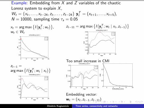
Example: Embedding from X and Z variables of the chaoticLorenz system to explain X ,Wt = {xt , . . . , xt−24, zt , . . . , zt−24} yTt = (xt+1, . . . , xt+5),N = 10000, sampling time τs = 0.05
xt = arg max{I(yTt ;wt
)},
wt ∈Wt
0 5 10 15 20 25
0.8
1
1.2
1.4
1.6
1.8
2embedding cycle 1
lags
MI
XZ
zt−1 =arg max
{I(yTt ;wt | xt
)}
0 5 10 15 20 250
0.2
0.4
0.6
0.8
1
1.2
1.4embedding cycle 2
lags
CM
I
XZ
zt−11 = arg max{I(yTt ;wt | xt , zt−1
)}
0 5 10 15 20 250
0.05
0.1
0.15
0.2
0.25
0.3
0.35embedding cycle 3
lags
CM
I
XZ
Too small increase in CMI
0 5 10 15 20 250
0.05
0.1
0.15
0.2embedding cycle 4
lags
CM
I
XZ
2 4 6 8 100
0.5
1
1.5
2
CM
I
Embedding cycles
Embedding vector:wt = (xt , zt−1, zt−11)
Dimitris Kugiumtzis Time series, connectivity and networks
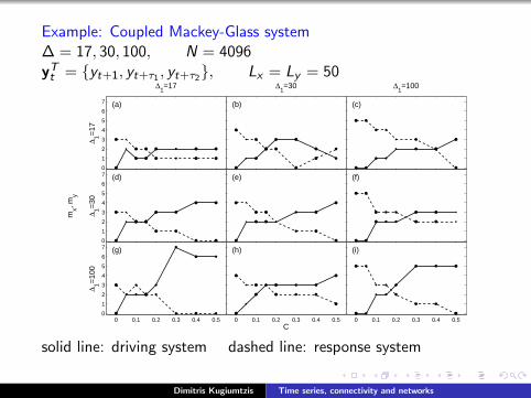
Example: Coupled Mackey-Glass system∆ = 17, 30, 100, N = 4096yTt = {yt+1, yt+τ1 , yt+τ2}, Lx = Ly = 50
0
1
2
3
4
5
6
7 (a)
Δ1=17
Δ 1=17
(b)
Δ1=30
(c)
Δ1=100
0
1
2
3
4
5
6
7 (d)
mx, m
y
Δ 1=30
(e) (f)
0 0.1 0.2 0.3 0.4 0.50
1
2
3
4
5
6
7 (g)
Δ 1=10
0
0 0.1 0.2 0.3 0.4 0.5
(h)
C0 0.1 0.2 0.3 0.4 0.5
(i)
solid line: driving system dashed line: response system
Dimitris Kugiumtzis Time series, connectivity and networks
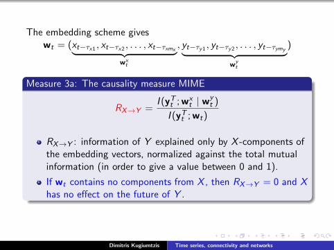
The embedding scheme giveswt = (xt−τx1 , xt−τx2 , . . . , xt−τxmx︸ ︷︷ ︸
wxt
, yt−τy1 , yt−τy2 , . . . , yt−τymy︸ ︷︷ ︸wyt
)
Measure 3a: The causality measure MIME
RX→Y =I (yTt ; wx
t | wyt )
I (yTt ; wt)
RX→Y : information of Y explained only by X -components ofthe embedding vectors, normalized against the total mutualinformation (in order to give a value between 0 and 1).
If wt contains no components from X , then RX→Y = 0 and Xhas no effect on the future of Y .
Dimitris Kugiumtzis Time series, connectivity and networks

driving system: X , response system: Y ,conditioning on system Z , Z = {Z1,Z2, . . . ,ZK−2}
The same non-uniform embedding scheme for explaining yTt fromvector of lags of all X ,Y ,Z1,Z2, . . . ,ZK−2,
Wt ={xt , . . . , xt−Lx−1, yt , . . . , yt−Ly−1, z1,t , . . . , z1,t−Lz−1, . . . , zK−2,t−Lz−1}
e.g., for K = 3, X ,Y ,Z :wt = (xt−τx1 , . . . , xt−τxmx︸ ︷︷ ︸
wxt
, yt−τy1 , . . . , yt−τymy︸ ︷︷ ︸wyt
, zt−τz1 , . . . , zt−τzmz︸ ︷︷ ︸wzt
)
Dimitris Kugiumtzis Time series, connectivity and networks

3b: The causality measure PMIME
RX→Y |Z =I (yTt ; wx
t | wyt ,w
Zt )
I (yTt ; [wxt ,w
yt ] | wZ
t )
RX→Y |Z : information of Y explained only by X -componentsof the embedding vectors, normalized against the mutualinformation accounting for the presence of wZ
t .
If wZt = ∅, then RX→Y |Z = RX→Y .
If wt contains no components from X , then RX→Y |Z = 0 andX has no direct effect on the future of Y .
Dimitris Kugiumtzis Time series, connectivity and networks

free parameters: T , LX , LY , LZ
T : as for any other “driver-response” measure
LX , LY , LZ : can be arbitrarily large (at the cost of longercomputations)when all variables are of the same type LX = LY = LZ = L
Three main advantages of PMIME
RX→Y |Z = 0 when no significant causality is present andRX→Y |Z > 0 when it is present [no significance test, no issueswith multiple testing!]
mixed embedding for all variables is formed as part of themeasure [it does not require the determination of embeddingparameters for each variable]
inclusion of more confounding variables only slows thecomputation and has no effect on statistical accuracy [no“curse of dimensionality” for any dimension of Z , only slowcomputation time]
⇒ good candidate for connectivity/causality analysisDimitris Kugiumtzis Time series, connectivity and networks
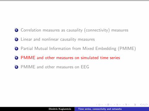
1 Correlation measures as causality (connectivity) measures
2 Linear and nonlinear causality measures
3 Partial Mutual Information from Mixed Embedding (PMIME)
4 PMIME and other measures on simulated time series
5 PMIME and other measures on EEG
Dimitris Kugiumtzis Time series, connectivity and networks

Example: linear coupled system
K = 5 linear Vector Autoregressive process, VAR(4) in 5 variables
x1,t = 0.4x1,t−1 − 0.5x1,t−2 + 0.4x5,t−1 + e1,t
x2,t = 0.4x2,t−1 − 0.3x1,t−4 + 0.4x5,t−2 + e2,t
x3,t = 0.5x3,t−1 − 0.7x3,t−2 − 0.3x5,t−3 + e3,t
x4,t = 0.8x4,t−3 + 0.4x1,t−2 + 0.3x2,t−2 + e4,t
x5,t = 0.7x5,t−1 − 0.5x5,t−2 − 0.4x4,t−1 + e5,t
[Schelter et al, 2006]
Network with directed linksCausality matrix
Dimitris Kugiumtzis Time series, connectivity and networks
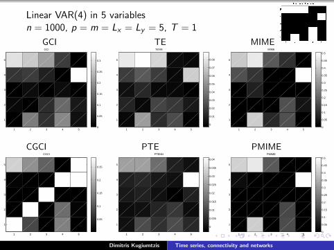
Linear VAR(4) in 5 variablesn = 1000, p = m = Lx = Ly = 5, T = 1
GCI TE MIME
1 2 3 4 5
1
2
3
4
5
GCI
0
0.05
0.1
0.15
0.2
0.25
0.3
1 2 3 4 5
1
2
3
4
5
TENN
0
0.01
0.02
0.03
0.04
0.05
0.06
0.07
0.08
1 2 3 4 5
1
2
3
4
5
MIME
0
0.05
0.1
0.15
0.2
0.25
0.3
0.35
0.4
0.45
0.5
CGCI PTE PMIME
1 2 3 4 5
1
2
3
4
5
CGCI
0.05
0.1
0.15
0.2
0.25
1 2 3 4 5
1
2
3
4
5
PTENN
0
0.005
0.01
0.015
0.02
0.025
0.03
0.035
0.04
1 2 3 4 5
1
2
3
4
5
PMIME
0
0.05
0.1
0.15
0.2
0.25
0.3
0.35
0.4
0.45
0.5
Dimitris Kugiumtzis Time series, connectivity and networks

Example: Nonlinear system - Henon coupled maps
K = 5 Henon coupled maps
x1,t+1 = 1.4− x21,t + 0.3x1,t−1
xi,t+1 = 1.4− (0.5C (xi−1,t + xi+1,t) + (1− C )xi,t)2 + 0.3xi,t−1
xK ,t+1 = 1.4− x2K ,t + 0.3xK ,t−1
coupling strength: C = 0, . . . , 0.9 [Politi & Torcini, PRL 1992]
Network withdirected links
Causality matrix(not symmetric)
Dimitris Kugiumtzis Time series, connectivity and networks

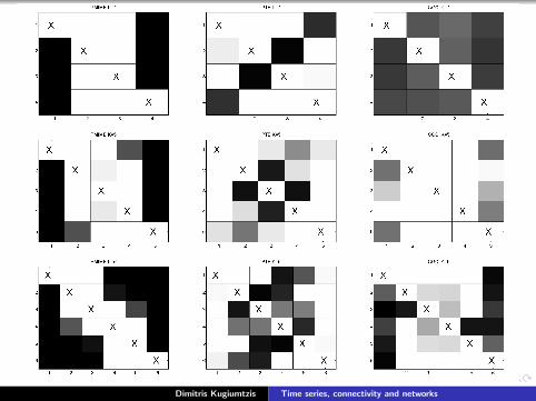
C = 0.0 n = 1024, p = 5, m = 2, L = 5, T = 1
GCI TE MIME
CGCI PTE PMIME
Dimitris Kugiumtzis Time series, connectivity and networks
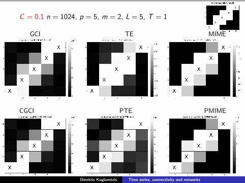
C = 0.1 n = 1024, p = 5, m = 2, L = 5, T = 1
GCI TE MIME
CGCI PTE PMIME
Dimitris Kugiumtzis Time series, connectivity and networks
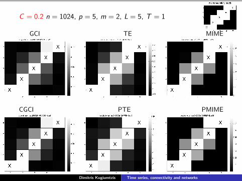
C = 0.2 n = 1024, p = 5, m = 2, L = 5, T = 1
GCI TE MIME
CGCI PTE PMIME
Dimitris Kugiumtzis Time series, connectivity and networks
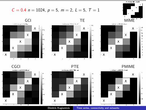
C = 0.4 n = 1024, p = 5, m = 2, L = 5, T = 1
GCI TE MIME
CGCI PTE PMIME
Dimitris Kugiumtzis Time series, connectivity and networks
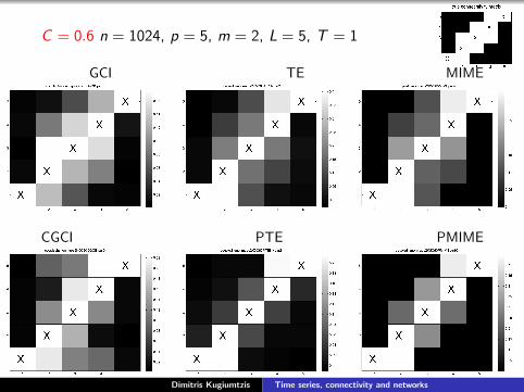
C = 0.6 n = 1024, p = 5, m = 2, L = 5, T = 1
GCI TE MIME
CGCI PTE PMIME
Dimitris Kugiumtzis Time series, connectivity and networks

C = 0.7 n = 1024, p = 5, m = 2, L = 5, T = 1
GCI TE MIME
CGCI PTE PMIME
Dimitris Kugiumtzis Time series, connectivity and networks
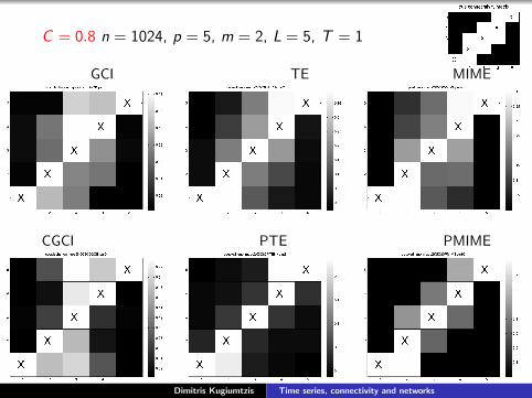
C = 0.8 n = 1024, p = 5, m = 2, L = 5, T = 1
GCI TE MIME
CGCI PTE PMIME
Dimitris Kugiumtzis Time series, connectivity and networks
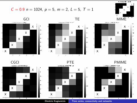
C = 0.9 n = 1024, p = 5, m = 2, L = 5, T = 1
GCI TE MIME
CGCI PTE PMIME
Dimitris Kugiumtzis Time series, connectivity and networks

K = 5, n = 1024, 100 realizations, PMIME (L = 5) compared topartial transfer entropy (PTE, m = 2) and conditional Grangercausality index (CGCI, p = 2)
Dimitris Kugiumtzis Time series, connectivity and networks
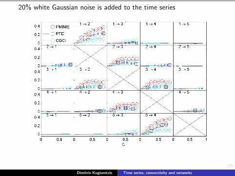
20% white Gaussian noise is added to the time series
Dimitris Kugiumtzis Time series, connectivity and networks
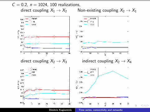
C = 0.2, n = 1024, 100 realizations,direct coupling X1 → X2 Non-existing coupling X2 → X1
direct coupling X2 → X3 indirect coupling X2 → X4
Dimitris Kugiumtzis Time series, connectivity and networks

Example: coupled Mackey-Glass
Coupled identical Mackey-Glass delayed differential equations
xi (t) = −0.1xi (t) +K∑j=1
Cijxj(t −∆)
1 + xj(t −∆)10for i = 1, . . . ,K
∆ = 20, C = 0.2, n = 2048, 100 realizations,
Dimitris Kugiumtzis Time series, connectivity and networks
Dimitris Kugiumtzis Time series, connectivity and networks

Mackey-Glass: true and estimated network
K = 5 True from PMIME (∆ = 20) from PMIME (∆ = 100)
K = 15 True from PMIME (∆ = 20) from PMIME (∆ = 100)
Dimitris Kugiumtzis Time series, connectivity and networks
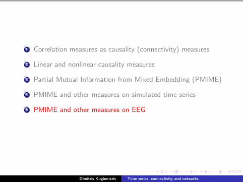
1 Correlation measures as causality (connectivity) measures
2 Linear and nonlinear causality measures
3 Partial Mutual Information from Mixed Embedding (PMIME)
4 PMIME and other measures on simulated time series
5 PMIME and other measures on EEG
Dimitris Kugiumtzis Time series, connectivity and networks

Transcranial Magnetic Stimulation (TMS)
Dimitris Kugiumtzis Time series, connectivity and networks

TMS-EEG: brain connectivity analysis
Jointly with Vassilis Kimiskidis, Medical School, AUTh
TMS: transcranial magnetic stimulation
How does TMS act on epileptic brain connectivity?
{X1,X2, . . . ,XK}: K EEG channels, each represents a (sub)system
Practical problems to overcome:
Application on small time windows ⇒ limited data size
scalp EEG ⇒ many channels ⇒ many variables in Z toaccount for
Brain system is complex: the connectivity measure has to deal
with
high dimensionalitynonlinearity?sensitivity on free parameters?
PMIME addresses all these problems!
Dimitris Kugiumtzis Time series, connectivity and networks

TMS-EEG data processing
Many issues related to processing of TMS-EEG data:
1 Rejection of corrupted EEG channels [by visual inspection,initially 60 channels]
2 Elimination of TMS artifact [forward-backward nearestneighbor smoothing]
3 Removal of artifacts [ICA ?]
4 Filtering [FIR, lowpass 0.3Hz, highpass 40Hz, order 60]
5 Mastoid reference, Re-referencing ?
6 Sampling frequency [downsampling from 1450 Hz to 200 Hz]
TMS was administered in blocks of 5 at frequency 3Hz or 5Hzafter epileptic discharges (ED) were visually detected.
Computation of PMIME was done on sliding windows
Dimitris Kugiumtzis Time series, connectivity and networks

Example: compare PMIME to other measures on EEG
One ED episode, totally 45 channels
Select randomly a subset of channels.
Compute the connectivity measures on the subset at eachsliding window
Compute average connectivity strength at each slidingwindow.
Repeat the steps above a number of times (here 12).
... for subsets of 5, 15, 25, 35 and once for 45 channels.
Dimitris Kugiumtzis Time series, connectivity and networks
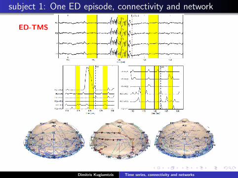
subject 1: One ED episode, connectivity and network
ED-TMS
Dimitris Kugiumtzis Time series, connectivity and networks
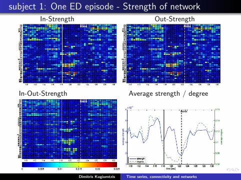
subject 1: One ED episode - Strength of networkIn-Strength Out-Strength
In-Out-Strength Average strength / degree
Dimitris Kugiumtzis Time series, connectivity and networks

subject 1: Many ED episodes
Average strength
Dimitris Kugiumtzis Time series, connectivity and networks
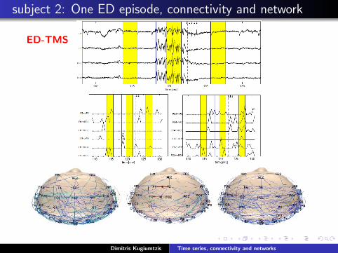
subject 2: One ED episode, connectivity and network
ED-TMS
Dimitris Kugiumtzis Time series, connectivity and networks

subject 1: One ED episode - Strength of network
In-Strength Out-Strength
In-Out-Strength Average strength / degree
Dimitris Kugiumtzis Time series, connectivity and networks
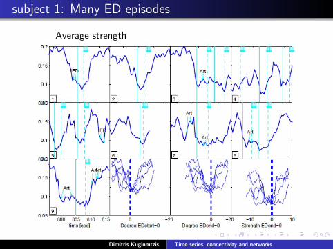
subject 1: Many ED episodes
Average strength
Dimitris Kugiumtzis Time series, connectivity and networks

Summary
Many measures of causality:best: these that can capture also nonlinear and direct causaleffects ...but practically hard to estimate reliably.
1 More advanced measures (nonlinear, direct effects) involvemore (and depend more on) free parameters.
2 Harder to establish statistical significance of the measureswhen many variables are present (many nodes in the network).
3 Statistical accuracy of the direct causality measures decreaseswith the number of confounding variables.
Dimitris Kugiumtzis Time series, connectivity and networks

References
Brandt PT & Williams JT (2007) Multiple Time Series Models, Sage PublicationsGourevitch B, Le Bouquin-Jeannes R & Faucon G (2006) “Linear and nonlinear causality between signals:methods, examples and neurophysiological applications”, Biological Cybernetics, 95: 349-369
Kraskov A, Stogbauer H & Grassberger P (2004) “Estimating Mutual Information”, Physical Review E, 69(6):066138
Papana A, Kugiumtzis D & Larsson PG (2011) “Reducing the bias of causality measures”, Physical Review E, 83:036207
Papana A, Kugiumtzis D & Larsson PG (2012) “Detection of direct causal effects and application in the analysis ofelectroencephalograms from patients with epilepsy”, International Journal of Bifurcation and Chaos, to bepublished
Schelter B, Winterhalder M, Hellwig B, Guschlbauer B, Luucking CH & Timmer J (2006) “Direct or indirect?Graphical models for neural oscillators”, Journal of Physiology, 99: 37–46
Schreiber T (2000) “Measuring Information Transfer”, Physical Review Letters, 85(2): 461–464
Vakorin VA, Krakovska OA & McIntosh AR (2009) “Confounding effects of indirect connections on causalityestimation”, Journal of Neuroscience Methods, 184: 152-160
Vlachos I & Kugiumtzis D (2010) “Non-uniform state space reconstruction and coupling detection”, PhysicalReview E, 82: 016207
Dimitris Kugiumtzis Time series, connectivity and networks