Time series forecasting used for real-timeanomaly detection on websites

author: Georgios Galvas

A thesis presented for the degree ofMSc Business Analytics

VU supervisor: Evert HaasdijkVU second reader: Sandjai Bhulai

Faculty of SciencesVrije Universiteit

Amsterdam, NetherlandsOctober 2016

ii

Abstract

The development of new methods of manipulating big data has made it possible for usersto constantly monitor the traffic behaviour of networks and websites, as well as enablingthem to manage and identify potential failures, or even intrusions. Due to the increasingcomplexity of computer networks and the great number of traffic-behaviour time-seriesdata generated in real time, manual inspection of the aforementioned by a human factoris rendered impossible. To deal with this problem, anomaly or failure detection modelshave been developed to identify potential deviations from pre-existing behavioural pat-terns. In the current paper we are presenting an anomaly detection model for identifyingpotential errors or failures in websites. Since the data of our metrics is time series data,we first introduce forecasting methods for time series. The focus will only be on the ex-ponential smoothing family techniques, especially the Holt-Winters model for time serieswith trend and seasonal variation, and Taylor’s models which are designed to account formultiple seasonality patterns. A comparison is made between these models in terms offorecasting accuracy and the results are presented. By using these forecasting models toindicate the expected future behaviour of our metrics, we have built an anomaly detec-tion model based on the observation that the residuals between the forecasts and actualvalues follow a Gaussian distribution centered around zero.

Tags: website performance, time series, exponential smoothing, Holt-Winters, Taylor,anomaly detection, Gaussian distribution.

iii

Declaration

I, Georgios Galvas, declare that this thesis titled, ’Real-time short-term time series fore-casting used for anomaly detection on websites’ and the work presented in it are my own.I confirm that:

� This work was done wholly during the master project Business Analytics.

� Where any part of this thesis has previously been submitted for a degree or anyother qualification at this University or any other institution, this has been clearlystated.

� Where I have consulted the published work of others, this is always clearly at-tributed.

� Where I have quoted from the work of others, the source is always given. With theexception of such quotations, this thesis is entirely my own work.

� I have acknowledged all main sources of help.

� Where the thesis is based on work done by myself jointly with others, I have madeclear exactly what was done by others and what I have contributed myself.

iv

Aknowledgements

This internship report was composed as a part of the Business Analytics Master programat the Vrije Universiteit of Amsterdam. The goal of the internship is to provide in depthexperience on the latest methods of today’s business environment, tackled with toolsfrom the field of Mathematics and Computer Science, the intersection of which togetherwith Business concepts composes the program of Business Analytics. The current thesisreport contains the results of my research performed at MeasureWorks, a company offeringservices and products having as its main goal the improvement of the performance of itsclients’ websites.

I would like to thank Jeroen Tjepkema, CEO and founder of MeasureWorks, for giv-ing me the opportunity to undertake my internship in the company, for his generosity,benevolence and trust in me. Furthermore, I am much obliged to Fernando Flores, datascientist and my supervisor in the company, for introducing me to the company’s work,for providing me with the background knowledge of the existing models and the datasetI worked on, together with his useful aid on technical matters of the software I used.Special thanks also to all the employees of Measureworks, for their willingness to helpwhenever needed. Finally, I would like to thank Evert Haasdijk, assistant professor andmy supervisor from the Vrije Universiteit, for his guidance and his useful recommenda-tions, essential to the fulfillment of my project.

Georgios GalvasOctober 2016,

Amsterdam

v

Contents

1 Introduction 11.1 Time series anomaly detection . . . . . . . . . . . . . . . . . . . . . . . . 11.2 Research questions . . . . . . . . . . . . . . . . . . . . . . . . . . . . . . 31.3 Organization . . . . . . . . . . . . . . . . . . . . . . . . . . . . . . . . . 3

2 Data insights and visualisation 52.1 Dataset general info . . . . . . . . . . . . . . . . . . . . . . . . . . . . . . 52.2 Seasonality patterns . . . . . . . . . . . . . . . . . . . . . . . . . . . . . 72.3 Public holidays . . . . . . . . . . . . . . . . . . . . . . . . . . . . . . . . 152.4 Missing values and outliers . . . . . . . . . . . . . . . . . . . . . . . . . . 19

3 Exponential smoothing forecasting methods 223.1 Simple and double exponential smoothing . . . . . . . . . . . . . . . . . 233.2 Holt-Winters method . . . . . . . . . . . . . . . . . . . . . . . . . . . . . 263.3 Taylor’s model for double seasonality . . . . . . . . . . . . . . . . . . . . 29

4 Experimental setup 334.1 Data engineering . . . . . . . . . . . . . . . . . . . . . . . . . . . . . . . 334.2 Parameter estimation . . . . . . . . . . . . . . . . . . . . . . . . . . . . . 374.3 Evaluation and comparison . . . . . . . . . . . . . . . . . . . . . . . . . . 38

5 Anomaly detection model 435.1 The Gaussian model . . . . . . . . . . . . . . . . . . . . . . . . . . . . . 435.2 Generating an alarm and evaluating performance . . . . . . . . . . . . . 475.3 Building robust forecasting models using the Gaussian anomaly detector 54

6 Conclusion 596.1 Further work . . . . . . . . . . . . . . . . . . . . . . . . . . . . . . . . . 60

Appendices 62

vi

vii

CHAPTER 1

Introduction

In a rapidly developing and highly technological world, “we are all now connected bythe Internet, like neurons in a giant brain” as Stephen Hawking stated. In this giantbrain, the websites give sense and meaning to its existence through the variety of edu-cational, communicational and entrepreneurial purposes they fulfill. Nowadays, websitesare central in the distribution of information, exchange of goods and services as well asthe monitoring process of everyday socioeconomical activities. Thus, they should havea consistent and high-speed performance in order to satisfy the users’ needs and reducediscontent. With the purpose of supporting websites’ smooth functionality, downfalls anderrors should be immediately identified and overhauled by anomaly detection tools. Thedemand for efficient anomaly detection tools becomes imminent since the new kinds ofdata (i.e. sensor data) emerge to mound on top of the growing volumes of the existingones.

MeasureWorks is a Web-performance solutions provider. For a wide range of Dutchcompanies, they provide performance tooling and consultancy to make websites faster,more reliable and ultimately deliver more conversion. The company, was founded in 2008,and for the past 2 years has been developing its own technology and products. Basedon a real time tracking mechanism they have built algorithms that can predict websiteoutrages, and track online sentiment to provide insight on these potential downfalls.This technology is currently available to a small set of clients. The current research isconducted on this downtime prediction platform, working with large sets of real timetracking data from a specific client.

1.1 Time series anomaly detection

When searching at the Oxford university dictionary about what an anomaly is, we findthe following definition:

anomaly something that deviates from what is standard, normal, or expected

Anomaly detection, as Dunning and Friedman [2014] highlight, is the science of ”spot-

1

ting the unusual, catching the fraud, of discovering the strange activity”. It is carriedout by a machine-learning program and is the method of finding any abnormalities inthe behaviour of a system or identifying outliers from a set of observations. Could itbe possible to identify abnormal observations based on the known and used methods?To effectively answer this, supervised machine learning techniques such as classificationand their ability of detecting anomalies must be called in question. The primary ideawould be to gather instances of the normal and abnormal kinds of data. This processwould facilitate the classifier to be trained efficiently in order to correctly classify futureobservations and subsequently identify the potential abnormalities.

However, by tackling the problem like this, a weakness is revealed: the inability toidentify new forms of anomalies previously unobserved. The process of retraining theclassifier, using some examples of this new irregularity, would have to be repeated, atime-consuming and costly procedure during which the classifier would be incapable ofdetecting these new kind of anomalies. Thus, the method of classification cannot beapplied due to the fact that the characteristics of an anomaly are generally not known.In a nutshell, according to the writings of Dunning and Friedman [2014]:

”Anomaly detection is all about finding what you don’t know to look for”

In contrast to other methods, anomaly detection tools are capable of identifying newforms of anomalies, previously unobserved. By knowing what normal is, they can defineanything different or ”far” from that normal to be labeled as anomalous. We can saythen that an anomaly is defined by contrast to what normal is. With this reasoning, touse the exact words of [Dunning and Friedman, 2014], the important aspect of anomalydetection can be summarized in the following words:

”Anomaly detection is based on the fundamental concept of modelingwhat is normal in order to discover what is not”

Consequently in our context, the challenge of identifying potential anomalies in theperformance of a website can be viewed as a problem regarding the creation of a modeldescribing a website’s ideal behaviour and its comparison to the observed one.

The data we have been working on, as is more extensively explained in the nextchapter, is time series data. According to Brutlag [2000], detecting anomalous behaviourin time series data consists of three stages, each one building on its predecessor:

1. An algorithm for predicting the values of a time series one time step ahead.

2. A measure of deviation between the predicted values and the observed values.

3. A mechanism to decide if and when an observed value or sequence of observedvalues is ’too deviant’ from the predicted value(s).

In the present paper we are only focusing on the class of exponential smoothing mod-els and not on the ARIMA (AutoRegressive Integrated Moving Average) when forecastingthe future values of a time series. The reason for this is due to the simplicity and trans-parency of the first, in combination with a greatly satisfying performance. Furthermore

2

the investigation focuses on single time series forecasting only (i.e. we do not consider anexplanatory variable for the time series yt), and the reason for that is that our main goalis to perform real time forecasting and anomaly detection. Thus ARIMA methods are notappropriate due to their computational complexity (see paper Au et al. [2011]). On theother hand, exponential smoothing methods, and especially the Holt-Winters method andits variations are known for their adaptable, robust character and their straightforwardimplementation.

1.2 Research questions

The model that MeasureWorks currently uses for time series forecasting is the SimpleExponential Smoothing or, as most commonly known, the Exponential Weighted MovingAverage (EWMA). Even though a robust forecasting method, EWMA produces accurateforecasts for constant level time series only, with no signs of seasonal repetitions. Oneof our objectives in this paper is, after a thorough investigation and understanding ofthe available dataset, to select and implement the most appropriate to the data model,the one that outperforms EWMA in terms of forecasting accuracy. Our first and mainresearch question then is the following:

1 According to the behavioural pattern of the measure variables,what is an appropriate forecast method for each metric and towhat extent does it improve the forecast accuracy of the alreadyexisting predictive model?

The main goal of Measureworks is to guarantee maximum website performance toits clients. Therefore, after the selection of the most appropriate time series forecastingtool for all the metrics that describe the good behaviour of a website, a method whichevaluates and distinguishes normal from abnormal behaviour is needed. This naturallyleads to the second research question we aim to answer:

2 How can we identify an appropriate method, based on the newforecasting model, to automatically detect anomalous behaviouron websites, and subsequently raise an alarm?

1.3 Organization

The paper is organized as follows: In chapter 2 we introduce the dataset, which is timeseries data for 81 days from a website of a Dutch company, and we investigate its features.Special interest is given in the seasonal patterns of each one of the different measurementvariables/metrics. Chapter 3 introduces the forecasting techniques, the one currently usedwhich we want to replace and the new models to be tested and compared, all belongingto the exponential-smoothing family of forecasting methods. In chapter 4 we evaluate

3

and compare the performance of all the new forecasting models. Chapter 5 describesthe creation and implementation of the anomaly detection model, which is based on theassumption of normally distributed forecasting errors. Finally, chapter 6 is a conclusiontogether with some ideas for future further improvement.

4

CHAPTER 2

Data insights and visualisation

The first and maybe most important step before building a model intended to perform aspecific task is to have a good understanding of the dataset of interest. Each dataset hasdifferent characteristics and the choice of the most appropriate model is closely relatedto the identification of these unique features. For that reason we start our investiga-tion with an explanatory data analysis before we delve into the details of selection andimplementation of the most appropriate for our case models.

2.1 Dataset general info

The dataset that was made available for the current thesis comes from the website of aDutch consumer and business finance company. It consists of time series data for almost81 days for the period between March 19 and June 7, for the year 2016. For this timeperiod we have a total of 108787 instances. The metrics of interest are analyzed in oneminute intervals, a practice also followed by Pena et al. [2013] when forecasting the trafficvolume of an IP network, due to the need of instant reaction when unusual behaviour ismonitored. Since we are concerned about finding evidence of any abnormal behaviour onwebsites, we choose the following two metrics which are indicative of the performance ofa website:

1. Number of pageviewsThe total number of users that viewed the website within each minute of the day.

2. Median pageload timeThe time that a website needs to load is defferent for every user, and mainly dependson the Internet connection. Among all the visitors of the website within a minute,we take the median of all these numbers - as a more robust location estimator - toindicate the median pageload time of the website for each minute of the day.

A complete day has 60 × 24 = 1440 minutes and consequently, since the measuringis performed every one minute, a daily cycle will have 1440 measurements or instances,and therefore a whole week should idealy consist of 1440× 7 = 10080 measurements. Foreasiness, we choose to view the dataset in terms of weeks. That way, the dataset can also

5

be described as being composed of 11 complete weeks and 4 seperate days. We make theconvention that a complete week starts from the midnight hour, i.e. 00:00, of a Mondayand ends to one minute before midnight , i.e. 23:59, of the Sunday of the same week.

By seperating the data set in terms of weeks, knowing the starting and finishing dateof each week we can find which weeks have missing data by counting the instances. Ontable of figure 2.1 below there is in detail the number of missing values of the entiredataset. Apart from these numbers, the table also includes the percentage of missingvalues with respect to the total expected number of instances for the specfic period,giving us a general view of how complete each week and consequently the whole datasetis.

Time period Date Numberof missingvalues

% of missing valueswith regard to timeperiod

First 2 days 19/3 - 20/3 61 2.1%Week 1 21/3 - 27/3 73 0.72%Week 2 28/3 - 3/4 5 0.05%Week 3 4/4 - 10/4 227 2.2%Week 4 11/4 - 17/4 39 0.39%Week 5 18/4 - 24/4 3124 31%Week 6 25/4 - 1/5 135 1.3%Week 7 2/5 - 8/5 259 2.6%Week 8 9/5 - 15/5 81 0.8%Week 9 16/5 - 22/5 2700 26.8%Week 10 23/5 - 29/5 12 0.12%Week 11 30/5 - 5/6 211 2.1%Last 2 days 6/6 - 7/6 926 62%

Figure 2.1: Table of missing values for the whole dataset

From the table of figure 2.1, the following important conclusions can be drawn: bysumming the total number of missing values and dividing it with the number of instancesideally expected for the specific time period, we find that the percentage of missing valuesfor the entire dataset is less than 7%. Unfortunately, most of these lay on the 5th and 9thweek, where 31% and 26.8% of the values of these weeks respectively are missing. Thistranslates in more than two complete days missing for each of these two weeks, whichmakes week 5 and 9 less informative than the rest of the weeks. In addition to that, thelast two days have 62% of the values missing, a high percentage to consider these daysvaluable for providing enough information.

6

2.2 Seasonality patterns

It is quite often the case that human activities show some form of repetition patterns.A brief look in the literature proves the cyclical nature of users’ behavior: the electricitydemand of a country examined by Souza et al. [2007], the number of mobile phone callsat a particular cell tower site investigated by Au et al. [2011], the number of call centerarrivals from Taylor [2010a] and the amount of traffic in TCP/IP based networks analyzedby Cortez et al. [2012] are just some of the many examples in which the cyclical characterof the human behaviour causes these measurements to exhibit several seasonality patterns.In this section we aim to reveal any seasonal patterns hidden in our dataset, by producingplots for the two different metrics of our interest.

Number of pageviews

We start by presenting plots for the total number of pageviews. The plots of the com-plete dataset for each one of the weeks can be found in the appendix at the end of thisdocumentation. Here we present only some of them, those that we consider to be moreindicative. For every graph that is produced within a period of time - whether this isfor a day, a week, several consecutive days or the entire dataset - the x-axis starts frommidnight hours 00:00 of the first day and ends at 23:59 of the last day. To protect theproprietary information of our clients, each time series in the graphs is scaled by a randomfactor.

On figure 2.2 a plot of the whole dataset for the metric number of pageviews is pro-duced. A first general observation is that the data appear to have a changing level, butnot an apparent increasing or decreasing trend. Furthermore, regarding the seasonal rep-etitions, it is not easy to make clear conclusions about presence of any seasonal patternsfor the metric. It seems though that there must be a daily pattern, due to the multiplespikes, each one indicating the peek during one day.

7

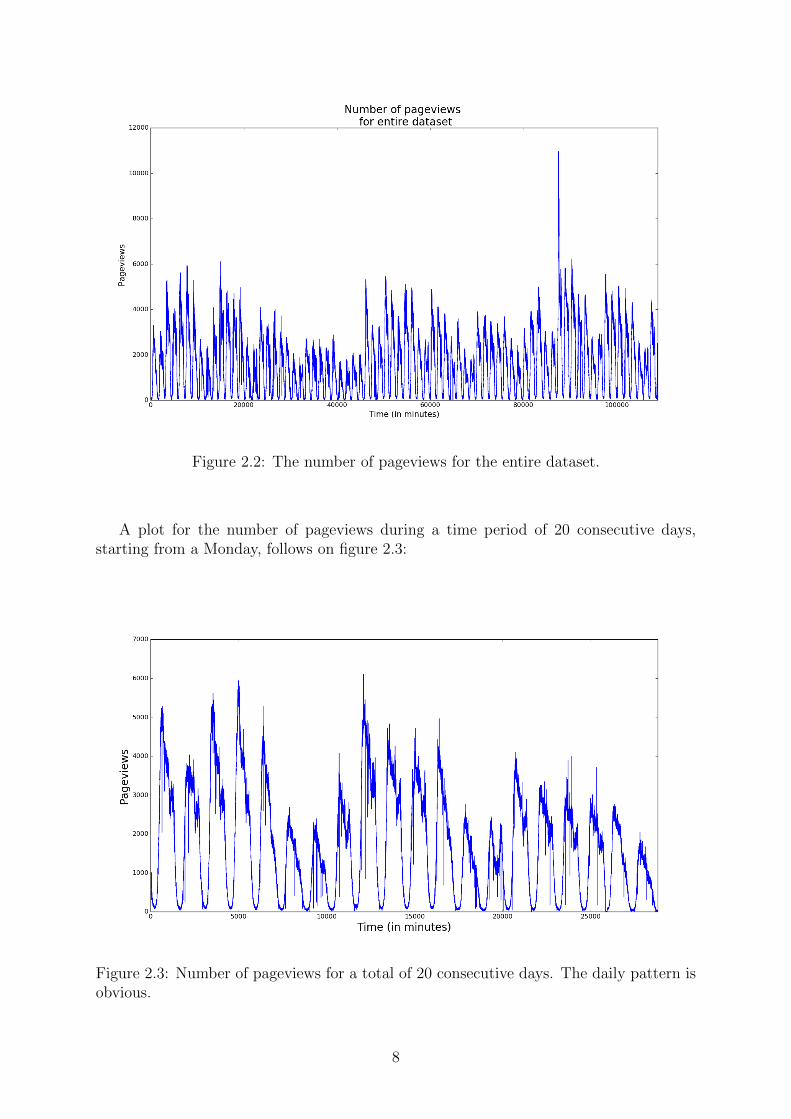
Figure 2.2: The number of pageviews for the entire dataset.

A plot for the number of pageviews during a time period of 20 consecutive days,starting from a Monday, follows on figure 2.3:

Figure 2.3: Number of pageviews for a total of 20 consecutive days. The daily pattern isobvious.

8

As we can see from figure 2.3, there are 20 peeks, each one for a seperate day whichindicates that indeed our data follow at least a daily pattern. The behaviour of the metricfor each day seems to be the same, the only apparent difference is the level it reaches -for some days the number of pageviews is higher and for others it is lower - but the dailycycle is obvious. To acquire some insight on the behavior of the users, we continue by aplot of the intra-day cycle of a normal weekday.

On figure 2.4 some general observations regarding the common patterns of the dailycycle for the weekdays can be made. The pageviews start increasing in the morninghours between 06:00am and 07:00am. The increase is vast up to around 10:00am, whereit reaches the maximum value of the day between 11:00 and 12:00. After this peek thecurve starts diclining - probably due to lunch time - until the time between 4:00pm and5:00pm. From that point a rapid decrease follows which can perhaps be attributed to thefact that it is the time that people leave their works, reaching a local minimum at around6:00pm. From this point there is an increase between 6:00pm and 7:30pm, followed by aconstant behavior of 2-3 hours, until 10:00pm when a rapid decline starts again.

Figure 2.4: Daily behavior of the metric ”number of pageviews” for a normal weekday.Two peeks are obvious, one in the morning and one in the evening: a global maximumreached at around 11:00 to 12:00 and a local one reached beween 19:30 and 22:00.

To see in a clearer view we produce a one-week plot about the total number ofpageviews, starting from Monday up to Sunday. The weekly pattern is easily seen fromthis plot in figure 2.5:

9

Figure 2.5: A whole week for the number of pageviews. This metric during weekdaysreaches a higher level compared to Saturday and Sunday.

From the weekly plot of figure 2.5, as well as figure 2.6 following, some importantrealizations can be made regarding the behaviour of this metric:

1. Week days from Monday to Thursday seem to have similar behaviour with eachother, same like the one explained before when describing the daily pattern of figure2.4: pageviews during these days appear to have two peeks, one global maximumtaking place in the morning hours followed by a local maximum occuring in theevening hours.

2. The last weekday before weekend, Friday, appears to show a relatively differentbehaviour than the rest of the weekdays: even though the morning peek occurs,just like the rest of the weekdays, the evening increase is of lower magnitude, almostnot existing. This could be attributed to the fact that users’ behaviour on Fridayevening is affected by the upcoming weekend.

3. Regarding the weekend, it is apparent that Saturdays and Sundays behave differ-ently than the weekdays, since they reach a lower level. Furthermore, they alsoseem to have differences between each other. Saturday appears to have a morningpeek followed by a notably smaller evening peek (quite similar to Friday’s eveningpeek, maybe a slightly more obvious). On the other hand, the Sunday morning andafternoon peeks seem to be of the same magnitude with each other.

From all the above, two important conclusions can be drawn regarding the seasonalitypatterns of the metric number of pageviews. This metric not only exhibits a daily seasonalpattern, but also a strong weekly pattern. In particular, its weekly behaviour could bedevided in four distinct categories: the weekdays between Monday and Thursday allbehaving in a very similar way, and Fridays, Saturdays and Sundays, each one forming aseperate category due to the different behaviour of their daily cycle.

10

Figure 2.6: The number of pageviews for the last 2 weeks of the dataset. Apparently ananomaly occured on the first Monday, which is the reason that the first daily cycle onthe current graph is different than expected.

Median pageload time

We continue with the second metric, the median pageload time and we plot the timeseries for the whole data set and for 20 consecutive days, starting from a Monday, justlike we did with the previous metric. From figures 2.7 and 2.8 one general but obviousobservation can be made: there are observations that are really higher in magnitude thanthe rest. This is clearly visible from the plot of the entire dataset.

Figure 2.7: The median pageload time for the entire dataset.

11

On the other hand, a daily pattern can be observed with easiness from figure 2.8,where the intra-day cycles are seen as different spikes.

Figure 2.8: The median pageload time for a total of 20 consecutive days.

To reveal if there is any weekly pattern, we plot the median pageload time for onewhole week, starting from the early hours of Monday to late midnight of Sunday.

Figure 2.9: The median pageload time for an entire week.

12

From figure 2.9 there is no apparent evidence that this metric exhibits a weeklyseasonal pattern. Unlike number of pageviews, the behaviour of median pageload timeseems very similar - if not the same - for all the days of the week. To ensure that thisis indeed the case, on figure 2.10 we plot the weekly behaviour of median pageload timefocusing only on the 200-400 range. It seems that there are slight differences betweenweekdays and weekends: the deviation in the weekends is higher, and the underlying levelof the metric takes lower values in weekends compared to weekdays.

Figure 2.10: Weekly seasonal patterns - even though weak - shown for a random weekfor the median pageload time. Weekends seem to deviate more, compared to weekdays.The differences between some weekdays and weekends are circled in red.

Regarding the intra-day cycle, we plot the behaviour of the median pageload time fora random day, a Wednesday, on figure 2.11. It is visible that between midnight hoursand the time around 8:00am the curve resigns a triangular movement: an increase startsa few minutes before the midnight hours, where it reaches a global maximum betweenthe early morning hours of 3:00am to 4:00am. From that point and forward the curvedeclines reaching a minimum value at around 8:00am, where it keeps a forthcoming steadybehavior until almost the end of the evening hours.

If we compare this behaviour with the one of the previous metric this seems contra-dicting to some extent, since these high values of the median pageload time are reachedexactly during the hours that the number of pageviews, are taking the lowest values pos-sible during the day, as we have seen from figure 2.4. A naive but reasonable enoughassumption would expect the pageload time of a website to be higher at the time wheremost of the users are visiting the website.

13

Figure 2.11: The intra-day cycle of the metric median pageload time, for a day of theweek of figure 2.9.

One important thing to point out from the graph of figure 2.11 is the high deviation ofthe values during the hours where the median pageload time is increrasing and decreasing,i.e. where the triangular curve is revealed - between 00:00am and 08:00am. On thecontrary, the steady behaviour taking place between 8:00am and 00:00am is characterizedby small deviations.

Figure 2.12: Plotting the metric median pageload time for two consecutive weeks.

14

To conclude, as regards the behaviour of median pageload time, there is strong evi-dence that this metric too has an intra-day cycle where its behaviour repeats after thecompletion of one day. Furthermore, apart from this daily seasonal cycle, it does seem toexhibit a weak weekly seasonality pattern. One other observation coming from the graphsis the high values that the outliers have, and the frequency this happens. Apparentlythis metric seems more prone to errors or falses.

2.3 Public holidays

One thing that we should take into account, which is clearly visible from the graphs, isthe effect that public holidays have on the metrics we study. The public holidays of theNetherlands for the year 2016 for the period of our dataset, are the following:

Holiday Date of holidayGood Friday Friday, March 25Easter Sunday Sunday, March 27Easter Monday Monday, March 28King’s Day Wednesday, April 27Liberation Day Thursday, May 5Whit Sunday Sunday, May 15Whit Monday Monday, May 16

For the whole data of the 9 complete weeks (after excluding the less informative data,as explained before), we plotted a graph comparing the behaviour of each of the sevendays of the week seperately. From these graphs, which can be found in the appendixin the end of the documentation, the effect of the public holidays is clear. Below is anindication example, for the case of Sundays for the metric number of pageviews :

As we explained before, the metric number of pageviews on Sundays has a differentbehaviour than the rest of the days, with two peeks of almost the same magnitude ap-pearing during midday and evening. As we can see from figure 2.13 though, this does nothold for holidays. On Easter Sunday, as well as on Whit Sunday we clearly see a changeon the pattern, namely the midday peek being almost double in size than the eveningpeek.

Similar realizations about the effect of holidays on the metrics can be made from theweekly plots. From figures 2.14, 2.15 and 2.16 we can also see the influence of holidayson the metric number of pageviews. Even though, as we observed previously, weekdaysfrom Monday to Thursday have a very similar pattern, the Easter Monday of week 2,the Wednesday of week 6 which is King’s day and the Thursday Liberation day of week7 take smaller values than the rest of the weekdays of the week they belong.

15

Figure 2.13: Daily cycle of pageviews for all Sundays

Figure 2.14: Users of the website are fewer during Easter Monday than the rest of theweekdays.

16

Figure 2.15: The impact of King’s day is obvious: pageviews on Wednesday reach a lowermaximum compared to the rest of the weekdays.

17

Figure 2.16: The fact that Thursday is Liberation day results in the number of pageviewsto reach a lower maximum compared to the rest of the weekdays.

On the contrary with the number of pageviews, the metric median pageload time doesnot show any significant relevance or connection to the Netherlands’ national holidays.From the graphs of the appendix we see that, for this metric, holidays behave similarlyas the rest of the days.

Figure 2.17: There is no sign of significant change on the behaviour of the median pageloadtime that can be attributed to public holiday.

18

2.4 Missing values and outliers

As it happens with most datasets, two are the main problems which prevent them frombeing declared as a good quiality dataset:

1. Missing values

2. Presence of Outliers

The fact that there are missing values in our data was proved and presented in thebeggining of this chapter. Namely, the problem lies mostly in weeks 5 and 9, which dueto the high amount of values that were not available, we concluded that no essentialinformation can be gained from these two weeks (see also fig 2.19).

Our historical data come from a website which - like most of the websites - hasexperienced several malfunctions in the past, and these malfunctions are depicted in thetwo metrics we study. For example, an unexpectedly low value of the number of pageviewsmay be the result of an error in the website, whereas a very high value could indicate apotential upcoming failure due to the high volumes of users. Furthermore, a high value ofthe metric median pageload time may be prognosticating a future anomalous behaviour.The presence of such unexpected values in our dataset, mostly know as outliers, is thennot surprising. We will talk about the importance of treating outliers in our contextof anomaly detection, together with methods of dealing with them, on the followingchapters.

Figure 2.18: Pageviews for a daily cycle containing abnormal values, highlighted with redcircles. These vertical lines which indicate sudden rapid increase could possibly result toan imminent website breakdown, while those unexpected falls could be attributed to aninstant collapse of the web page.

19

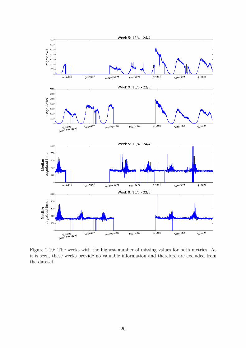
Figure 2.19: The weeks with the highest number of missing values for both metrics. Asit is seen, these weeks provide no valuable information and therefore are excluded fromthe dataset.

20

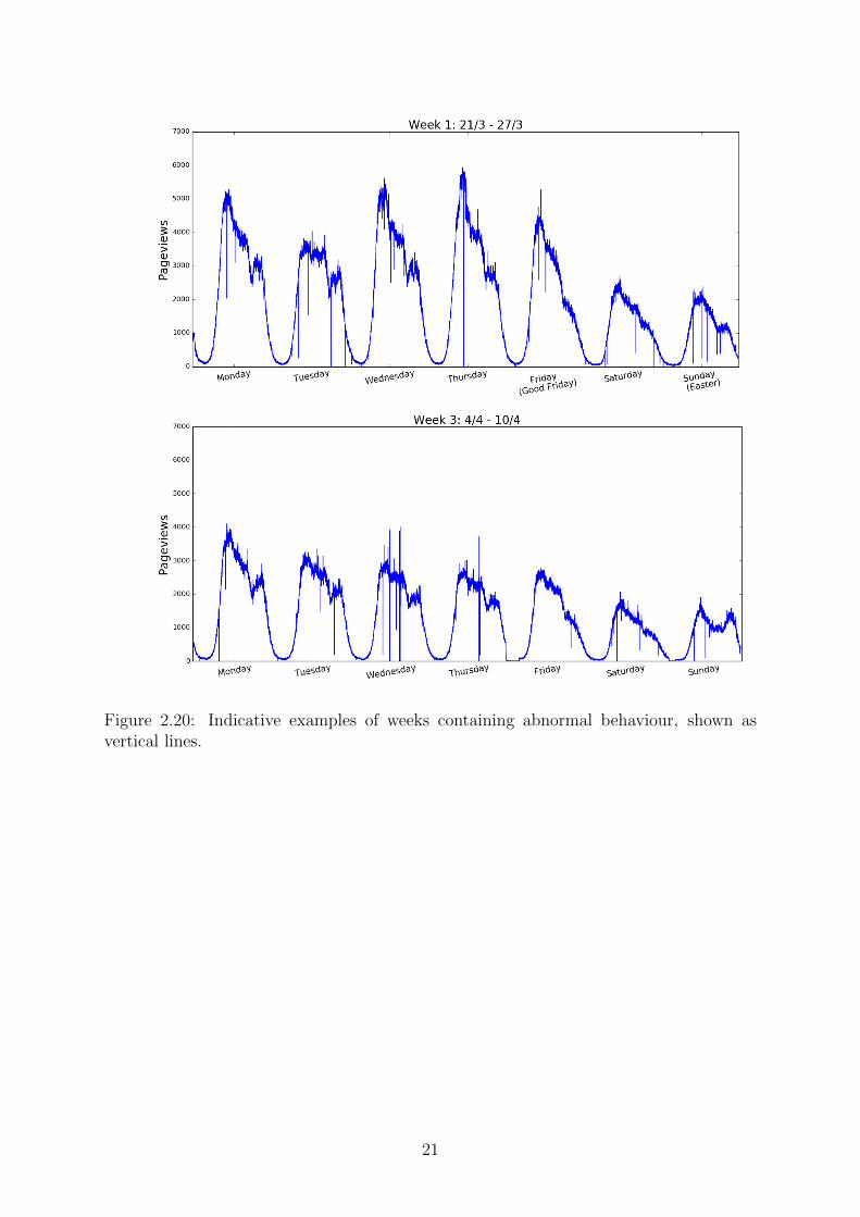
Figure 2.20: Indicative examples of weeks containing abnormal behaviour, shown asvertical lines.

21

CHAPTER 3

Exponential smoothing forecasting methods

Consider a time series {yt}, i.e. data measured in equally spaced points in time, andsuppose we want to make estimations about future values. For a start, lets assume thatthis time series does not show any form of trend or seasonality, i.e. no constant increase ordecrease nor any pattern of repetition, just random inherent variation which depends onfactors that we cannot see or understand. In mathematical terms, this can be expressedas

yt = c+ ε

where yt is the value of the time series at time t, c is the constant that determines thelevel of the time series and ε is the noise - this random inherent variation - with a meanof zero and variance of σ2.

Given this time series, our first attempt to forecast the future would be the simpleaverage of these values. Since the data show no trend or seasonality, they tend to gatheraround the mean and therefore the simple average seems the most plausible forecast tobegin with. This simple forecasting technique, though naive, takes into account all theavailable historical data and thus has the advantage of exploiting all information aboutpast behaviours.

There may be cases where the context of the problem suggests that only recent valuesreally play an important role in predicting the future. As an example consider the priceof a stock. Knowing the price of the stock one year ago provides little or no informationabout its future behaviour. In these cases we could agree that taking the mean of thelast k values, known as the k-period moving average - where k is to be determined - couldgive more accurate predictions than the simple average.

Furthemore, another possible technique would be to use the weighted average, i.e. toconsider all the previous values but give different weight to each one of them: biggerweight to data points that are closer to today in terms of time, and less weight to valuesthat are further in the past. By doing so, we have the advantages of both precedingmethods: we consider all the information we have from the historical data and at thesame time we give more importance to recent than to past information.

Another option would be to consider not the whole dataset but part of it, lets saythe last k values, and assign different weights to each data point on the same reasoning

22

as we explained before in the weighted average. This method is known as the k-periodweighted moving average and, even though by excluding the very old values we lose somepast information, it can produce accurate results in the cases where only recent past isbelieved to be informative.

The preceding forecasting methods, simple as they look, they raise some importantquestions: Can we determine k, the number of values that is informative enough toconsider when predicting future values? In each context and dataset this number willbe different and it seems difficult to choose a specific value other than an arbitraty one.At the same time, if we take all information into consideration and give more weight torecent than far-distant in time values, how can we determine the rule under which toassign the weights to each of the data points?

3.1 Simple and double exponential smoothing

The simple exponential smoothing method, also known as Exponential Weighted MovingAverage (or shortly EWMA) is a measure of central tendency that can be used to makevery accurate predictions for constant-level time series with no seasonality. The EWMAis a simple method that uses all the available historical data and assigns to them weightsdepending on how recent they are. These weights decrease exponentially as we considerdata points of the further past.

From now on and until the rest of the paper we denote with yt the forecast of thetime series at time t and with yt the actual true value at time t. Given this convention,the EWMA can be described in mathematical terms as follows:

yt+1 = α · yt + (1− α) · yt (3.1)

where α is the smoothing parameter with the restriction that 0 ≤ α ≤ 1.As we can see the only value that identifies EWMA is the parameter α, which can

intuitively seen as a measure of the impact of the last measurement - the greater the α,the greater the impact of the last measurement, the lower the value of α the better themodel ”remembers” the values of the distant past.

By placing the values of the forecasts in formula 3.1 and working recursively we getthe following alternative formula:

yt+1 = α · yt + α(1− α) · yt−1 + α(1− α)2 · yt−2 + ...+ α(1− α)t−1 · y1 + (1− α)t · y1(3.2)

which can also be written

yt+1 =

(t−1∑n=0

α(1− α)n · yt−n

)+ (1− α)t · y1 (3.3)

From formula (3.2) it is more clear that EWMA uses all the past available data inorder to make predictions for the future.

23

We can easily verify that the weights in equation 3.2 add up to one:(t−1∑n=0

α · (1− α)n

)+ (1− α)t = α ·

(t−1∑n=0

(1− α)n

)+ (1− α)t+1

= α · (1− α)t − 1

(1− α)− 1+ (1− α)t

= 1− (1− α)t+1 + (1− α)t+1

= 1

Component form

We now present an other alternative representation of the Simple Exponential Smoothing,which will also be particularly useful in the coming sections when we discuss about timeseries with trend and seasonality. According to Hyndman and Athanasopoulos [2013], inthis simple case of constant level time series with no seasonal patterns, we can ”break”the predictions in two equations, the forecast equation and the level smoothing equation:

level smoothing equation: `t = a · yt + (1− α) · `t−1 (3.4)

forecast equation: yt+1 = `t

The forecasted value at the next time step is equal to the estimated level on theprevious time step, where the level is a weighted average of the actual value and theestimated level computed up to and including the previous time instant.

Initialization

As equation (3.1) reveals, the forecast at time t+1 is equal to a weighted average betweenthe most recent observation yt and the most recent forecast yt. Moreover, looking atequation (3.2) and specifically on the last term, we can see that the initial value y1 att = 1 needs to be determined before we are able to make the first forecast.

Some initialization techniques are, either to set

`0 = y1

or to set the intial forecast value equal to the mean of the sample, i.e.:

`0 =1

T·

T∑t=1

yt

considering that our sample consists of values measured up to time T , starting fromt = 1.

24

Double exponential smoothing

It may be the case that a time series shows some increasing or decreasing behaviourregarding the average value it takes as it evolves in time. We then say that the timeseries shows some form of trend and the technique we use is known as double exponentialsmoothing or - by the name of the mathematician that developed it - Holt’s linear trendmodel.

The component form of Holt’s model will be the same as the one of the simple expo-nential smoothing with only difference that a second smoothing equation for the trendis added. Considering then that we have a sample of T in number time series valuesy1, y2, ..., yT , the smoothing and forecast equations of Holt’s model will be:

level smoothing equation: `t = α · yt + (1− α) · (`t−1 + bt−1)

trend smoothing equation: bt = β · (`t − `t−1) + (1− β) · bt−1 (3.5)

forecast equation: yt = `t−1 + bt−1, for t = 1, 2, ..., T.

When forecasting future values, i.e. values that we don’t have data measured at thetime instances, then the prediction is given by the future-forecast equation below:

yT+h|T = `T + h · bTwhere h = 1, 2, 3, ... is the step which we want to forecast further in the future startingmeasured from time T and forth, which from now on and for the rest of the paper wewill refer to it as forecast horizon or lead time and denote it by h. Using the notationof Hyndman and Athanasopoulos [2013], yT+h|T is the forecast for time T + h, where Tis the time of the last observed value of the time series, or from a statistical perspectivethe size of the data sample.

From equations (3.5) we can see that both the level and trend components need tobe initialized. We will talk about how we determine these initial values `0 and b0 in thenext section when describing the Holt-Winters model.

25

3.2 Holt-Winters method

The Holt-Winters method (HW), named after its inventors, is a continuation of Holt’smodel for a time series with a linear trend that also takes into account seasonal patterns,and was proposed by Holt’s student, Peter Winters in 1960 [source: Wikipedia]. In thismethod, at every time step estimates for the level, trend and seasonality components arerevised, which also justifies the name of triple exponential smoothing.

There are two different versions of the Holt-Winters method, for the two differentforms of seasonality patterns that define the model: the additive and the multiplicativeform. In its additive form, which we present first, the change of the seasonal fluctuationbetween two successive seasonal factors differ by a constant number, while in its multi-plicative form this change is a percentage and thus for greater values the change of thesuccessive cycle will be greater.

Additive model

forecast equation: yt = `t−1 + bt−1 + st−m

level smoothing equation: `t = α · (yt − st−m) + (1− α) · (`t−1 + bt−1)

trend smoothing equation: bt = β · (`t − `t−1) + (1− β) · bt−1 (3.6)

seasonality smoothing equation: st = γ · (yt − `t) + (1− γ) · st−m

for t = 1, 2, ..., T .The future forecast equation for h−time steps forward in the future since the time of

the last observed value will be

yT+h|T = `T + h · bT + sT+h−m, h = 1, 2, 3, ...

where m is the periodicity of one whole seasonal cycle, i.e. the number of time stepsof one full season. In our case where the measuring is done every one minute, if we wereto consider Holt-Winters model assuming daily seasonality, then m = 1440 while for thecase of weekly seasonal data this would be equal to m = 10080. We refer to m from nowon as length of the seasonal cycle and by the term ”seasonal cycle” we denote any patternthat repeats (with variation) periodically.

26

Multiplicative model

forecast equation: yt = (`t−1 + bt−1) · st−m

level smoothing equation: `t = α ·(

ytst−m

)+ (1− α) · (`t−1 + bt−1)

trend smoothing equation: bt = β · (`t − `t−1) + (1− β) · bt−1 (3.7)

seasonality smoothing equation: st = γ ·(yt`t

)+ (1− γ) · st−m

where t = 1, 2, ..., T .The forecast equation for h−time steps ahead in the future since the time of the last

observed value will be

yT+h|T = (`T + h · bT ) · sT+h−m, for h = 1, 2, 3, ...

The three smoothing parameters of the Holt-Winters model are:

α = the level parameter

β = the trend/slope parameter

γ = the parameter for the seasonal cycle

which follow the restriction of0 ≤ α, β, γ ≤ 1

Initializing Holt-Winters method

For the first method on how to initialize the Holt-Winters model we will need at leasttwo full seasonal cycles and, according to Hyndman and Athanasopoulos [2013] and RobJ Hyndman and Wheelwright [1997], is as follows:

The initial level component will be the average of the values of the first seasonal cycle.The initial slope/trend component will be the average of all the m-slopes computed inthe first two seasonal cycles. Finally, the initial seasonality components at each timeperiod for the additive case will be the observation minus the initial level and for themultiplicative case it will be the observation devided by the initial level. In mathematicalnotation, this initialization method can be summarized as follows:

27

initial level component: `0 =y1 + y2 + ...+ ym

m

initial slope component: b0 =

∑2mt=m+1 yt −

∑mt=1 yt

m2

(3.8)

initial seasonal component: si = yi − `0, additive case

si =yi`0, multiplicative case

for i=1,2,...,m.

28

3.3 Taylor’s model for double seasonality

So far we have described methods for forecasting time series, all belonging to the ex-ponential smoothing family of forecasting methods. For constant level time series withno seasonality we have showed that EWMA is adequate for forecasting, Holt’s lineartrend method is capable of predicting time series that show some form of linear trend,and finally the Holt-Winters method is used for times series with trend and seasonality.Furthermore we have noted that Holt-Winters, even though a very powerful and robustmethod for forecasting, that stays strong even now more than 50 years after its devel-opement, it takes into account one single seasonal pattern with seasonal cycle of lengthequal to m periods. But in real life problems, particularly in the business field, it is quitecommon that time series exhibit multiple seasonal patterns.

In his paper, Taylor [2003] further improved the work of Holt and Winters, allowing theinclusion of one seasonal cycle nested within another bigger one. In his proceeding paper,Taylor [2010b] extended his earlier work by presenting a model for forecasting a timeseries with intraday, intraweek and intrayear seasonal cycles. The philosphy underlyinghis theory is mainly adding one smoothing equation for each different type of seasonality.

Our data, as examined on the previous chapter, exhibit at least two seasonal patterns:daily and weekly. Consequently, in the current paper we seek to capture only these twoseasonal patterns, and thus here we only introduce Taylor’s model for double seasonalitywhich we refer to as Taylor’s double seasonal exponential smoothing method or shortlyTaylor’s Double Seasonal model.

Additive method

Similar to the case of Holt-Winters, there are two versions of Taylor’s DS model dependingon the form of seasonality in the data. In its additive form which we present first, theseasonal variation of the time series is not affected by the level of yt. In the state spaceequations below, this results in the fact that the seasonal and trend components enterthe forecasting equation in an additive manner:

forecast equation: yt = `t−1 + bt−1 +Dt−m1 +Wt−m2

level equation: `t = α · (yt −Dt−m1 −Wt−m2) + (1− α) · (`t−1 + bt−1)

trend equation: bt = β · (`t − `t−1) + (1− β) · bt−1daily seasonality : Dt = γ · (yt − `t −Wt−m2) + (1− γ) ·Dt−m1 (3.9)

weekly seasonality : Wt = δ · (yt − `t −Dt−m1) + (1− δ) ·Wt−m2

where t = 1, 2, ..., T . The forecast equation for predicting h−time steps ahead is thefollowing:

yT+h|T = `T + h · bT +DT+h−m1 +WT+h−m2

29

Multiplicative method

On the other hand, when the level of the time series affects the variation caused byseasonal factors, causing larger seasonal variation at higher values of yt, the multiplicativeversion is appropriate:

forecast equation: yt = (`t−1 + bt−1) ·Dt−m1 ·Wt−m2

level equation: `t = α ·(

ytDt−m1 ·Wt−m2

)+ (1− α) · (`t−1 + bt−1)

trend equation: bt = β · (`t − `t−1) + (1− β) · bt−1

daily seasonality : Dt = γ ·(

yt`t ·Wt−m2

)+ (1− γ) ·Dt−m1 (3.10)

weekly seasonality : Wt = δ ·(

yt`t ·Dt−m1

)+ (1− δ) ·Wt−m2

where t = 1, 2, ..., T .

future-forecast equation: yT+h|T = (`T + h · bT ) ·DT+h−m1 ·WT+h−m2

where h = 1, 2, 3, ... defines the h−time steps forward prediction.

Initializing Taylor’s Double Seasonal model

In his paper about forecasting and anomaly detection of network traffic, Szmit and Szmit[2012] use an arbitrary method to initialize the level, trend, and the daily and weeklyseasonal components specifically for the additive case:

`0 = y1

b0 = 0

D0,1 = D0,2 = ... = D0,m1 = 0 (3.11)

W0,1 = W0,2 = ... = W0,m2 = 0

The corresponding initialization method for the multiplicative case would then be

`0 = y1

b0 = 1

D0,1 = D0,2 = ... = D0,m1 = 1

W0,1 = W0,2 = ... = W0,m2 = 1

30

Another initialization method is proposed by Taylor [2003] when forecasting electricitydemand with multiplicative daily and weekly seasonality, which is also implemented onthe paper of Jalil et al. [2013], and uses simple averages of the first few data observations.Adapted to our sesonality characteristics where the length of the daily cycle is m1 = 1440and the length of the weekly cycle is m2 = 10080, these initial components were chosenas follows:

• The initial trend, b0, was chosen as the average of (1) 110080

of the difference betweenthe mean of the first 10080 and second 10080 observations, and (2) the average ofthe first differences for the first 10080 observations.

• The initial level, `0, was chosen as the mean of the first 20160 (= 2 × 10080 )observations minus 10080.5 times the initial trend, i.e.

`0 =1

2m2

·2m2∑t=1

yt − (m2 + 0.5) · b0

• The initial values for the within-day seasonal index, Dt, were set as the average ofthe ratios of actual observation to 1440-point centered moving average, taken fromthe corresponding minute in each of the first seven days of the time series.

More specifically, the nth component of the initial daily index D0, which correspondsto the nth minute of the day, n ∈ [1, 1440], will be

1

7·

7∑k=1

yn+(k−1)·1440

mean of the kthday of the first week

• The initial values for the within-week seasonal index, Wt, were set as the averageof the ratios of actual observation to 10080-point centered moving average, takenfrom the corresponding minute on the same day of the week in each of the firsttwo weeks of the time series, devided by the corresponding initial value of thesmoothened within-day seasonal index, Dt.

In mathematical terms, the nth component of the initial weekly index W0, whichcorresponds to the nth minute of the week, n ∈ [1, 10080], will be

1

2· 1

D(n mod 1440)

·2∑

k=1

yn+(k−1)·10080

mean of the kth week

where (n mod 1440) is the modulo operation, i.e the remainder of the Euclideandivision of n by 1440.

The corresponding initialization method for the additive case would produce the sameinitial level and trend component, while the initial seasonal components would be

31

1

7·

7∑k=1

(yn+(k−1)·1440 − [mean of the kthday of the first week]

)for the within-day seasonal index, and

1

2·

2∑k=1

(yn+(k−1)·10080 − [mean of the kth week]−D(n mod 1440)

)for the within-week seasonal index.We refer to this initialization method for the two different cases as (3.12). The initial-ization method influences the values of the smoothing parameters. How accurate thepredictions on the first days or weeks, which is mainly influenced by the initializationmethod, determines whether the smoothing parameters will be close to zero or close toone.

The smoothing parameters

The values that characterize the performance of this model are the smoothing parameters,which are the following:

α = the level parameter

β = the trend/slope parameter

γ = the parameter for the small seasonal cycle (daily in our case)

δ = the parameter for the bigger seasonal cycle (weekly in our case)

which follow the restriction of

0 ≤ α, β, γ, δ ≤ 1.

These four smoothing parameters define how much weight the components will giveto the recent observations and how much to those from the distant past, before theyget updated. As an example consider the daily seasonal component Dt. The value of γwill define whether for the update of this component more weight will be given in theseasonal variation between the minute t of the current day and the time instant t of theprevious day (when δ is close to 1) or whether for this computation the variations betweenconsecutive days belonging in the distant past are considered more informative, and thusγ will take a lower value, close to 0.

Furthermore, the weekly seasonal component Wt, where 1 ≤ t ≤ 10080, describesthe seasonal variation between a specific day of a week and the same weekday of theprecedeing week, for this particular minute t. A high value of δ would mean that for thecomputation of this Wt more weight is given in the variation of this specific time instantbetween the current and the precedent week than in the variation of the precedent weeks.Similarly for the trend parameter, a very high value of β - close to one - translates into asystem where for computating the trend in the dataset more weight is given in the changeof the underlying level between the present and one time step ago, that the trend as wascomputed from the past observations.

32

CHAPTER 4

Experimental setup

After a thorough investigation of the properties of the available dataset in chapter 2 andthe explanation of the theory behind the exponential smoothing forecasting techniquesin chapter 3, we move on to the implementation of these techniques in the dataset, whichis the topic of the current chapter. Apart from the implementation details and a briefdescription of the obstacles found, together with solutions proposed, we also present waysof evaluating the accuracy of the proposed models, as well as a comparison between them.As with most datasets, there are mainly two types of problems: the missing values andthe outliers.

4.1 Data engineering

Before we proceed to the evaluation and comparison of the models, we first prepare thedata set. This includes a method on treating the missing values, whether ouliers occur,how informative they are and how to handle them, and finally defining what part of thedataset will be used for training and what part for testing the models.

As we have seen in Chapter 2, the sample data we work on show daily and weeklyseasonality patterns for both median pageload time and number of pageviews. Because ofthe presence of abnormal points in the dataset, which we are interested in detecting withour anomaly detection model described in the following chapter, as well as the presenceof missing values, the dataset needs to be ”cleaned”.

The dataset is large enough, and so choosing to exclude weeks 5 and 9, together withthe first and last two days when training the model should not be a problem (see table offigure 4.4. If doing so, the percentage of the missing values for this new dataset yieldedfrom the original one, which consists of 9 complete weeks in total, would be around 1%,making this dataset even more appropriate to work with. However, by excluding the twocomplete weeks leaves us with discontinuous time series, since the behaviour of the 6thweek for example will follow that of the 4th week, and not the 5th as it should have been.This discontinuity of the time series would cause problems when training the model,especially when there is a considerable trend in the dataset.

In graph 4.1 we plot the metric number of pageviews for weeks 3, 4 and 6, in the samegraph. We see that for weeks 3 and 4 the level of the series, when looking at each of the

33

two weeks independently, is quite similar. However, this does not hold when looking atweeks 4 and 6. The underlying level of the time series seems to rapidly increase duringthe transition from week 4 to week 6, making us assume that, by not considering week 5when training the model we fail to capture the trend in the data - if any - leading to thetrend component and subsequently the trend parameter β to be distorted when searchingfor the optimal smoothing parameters.

Figure 4.1: The big change in the level of the time series between weeks 4 and 6, mayindicate that the discontinuity of the time series caused by excluding week 5 could leadto problems while training the models, making our performance results less reliable.

Figure 4.2: The difference between the underlying level of week 8 and week 10 mayindicate that week may contain valuable information

From graph 4.2 it is also clearly seen that weeks 7 and 8 seem to resemble each other interms of their underlying level while week 10 is considerably different, which may denotepotential missing information of the dataset that the exclusion of week 9 may cause. Onthe other hand from figure 4.3, it is visible that the change of the level between consecutiveweeks is not always increasing or decreasing smoothly. This rapid change between theunderlying level of some successive weeks can be attributed to external factors which are

34

not known and will not be investigated in the current documentation, or probably to theexistence of other extra seasonal patterns. The data seem to have a changing level ratherthan a trend, and so we conclude that the exclusion of weeks 5 and 9 from our datasetwill not have a big effect on the computation of the trend components, nor on parameterestimation of the forecasting models.

Figure 4.3: The number of pageviews for the entire dataset.

Time period Date Numberof missingvalues

% of missing valueswith regard to timeperiod

First 2 days 19/3 - 20/3 61 2.1%Week 1 21/3 - 27/3 73 0.72%Week 2 28/3 - 3/4 5 0.05%Week 3 4/4 - 10/4 227 2.2%Week 4 11/4 - 17/4 39 0.39%Week 5 18/4 - 24/4 3124 31%Week 6 25/4 - 1/5 135 1.3%Week 7 2/5 - 8/5 259 2.6%Week 8 9/5 - 15/5 81 0.8%Week 9 16/5 - 22/5 2700 26.8%Week 10 23/5 - 29/5 12 0.12%Week 11 30/5 - 5/6 211 2.1%Last 2 days 6/6 - 7/6 926 62%

Figure 4.4: Table of missing values for the whole dataset. Due to the high amount ofmissing values, we choose to exclude weeks 5 and 9, as well as the first and last two days,since we chose to work with complete weeks.

35

Since we are dealing with time series and each value is used for the forecast of thenext time step, it is invalid to not consider the values of all the minutes during each day.None of the models can tolerate gaps in the series - they need to use observations for eachminute of the day, for all the weeks. That is why we need to fill in the all the missinginstances with a number. In the present moment we fill in the missing values with theaverage of the preceding and proceeding available observation. Moreover, concearning theoutliers, we do not replace them with other, more ”normal”, values. In this initial modelcomparison we only deal with the missing values, and later we will present a method foridentifying and replacing the anomalous values, together with the impact of this on themodels’ performance.

Train and test set

To start with, we note the following: in order to produce an unbiased estimate of theperfomance of the models on unseen data, we will not consider how well a model fits thehistorical data. The accuracy of forecasts can only be determined by considering how wella model performs on new data that were not used when estimating the model. For thisreason, it is a common practice among the statisticians and researchers of the forecastingcommunity to devide the available initial dataset into two subsets: the train set and thetest set.

The train set is used for building or training the models, which mainly means definingthe optimal parameters for this model, i.e. the parameters that better describe thebehaviour of the available historical data. In our case, this is equivalent with definingα, β and γ in the case of the Holt-Winters or defining α, β, γ and δ in the case of Taylor’sdouble seasonal model.

Furthermore, after training the model, or - as it sometimes said - after tuning themodel parameters, we are to test how well the model performs with these optimal pa-rameters. To do that, we use an appropriate accuracy measure - depending on thecircumstances and dataset - which in principle is measuring the forecast error, i.e. thedeviation of the forecasts from the actual values. It is important that this evaluation isdone in observations that were not used to define the parameters of the model, and so,we use the test set for this purpose.

As a rule of thumb, adopted also by Hyndman and Athanasopoulos [2013], the 80%-20% rule is used, which requires the 80% of the dataset to be used as train set and theremaining 20% as test set.

Set Week % of entire datasettrain set 1, 2, 3, 4, 6, 7, 8 78%test set 10, 11 22%

Table 4.1: The partition of our dataset into a train and a test set follows the 80%-20%rule of thumb.

36

4.2 Parameter estimation

We explained before that the smoothing parameters depict how much ”memory” themodels should have, i.e. how far in the past they should look when considering historicalobservations for making predictions about the future. A big value of a parameter - avalue closer to 1 - means that the model is taking more recent observations in higheraccount than past observations. On the contrary, a parameter value close to zero makesthe model consider more the observations of the past than the more recent ones.

One common practice for selecting the optimal smoothing parameters from the avail-able historical data is to use a data-driven procedure optimizing a certain criterion. Forevery combination of the parameters α, β and γ for Holt-Winters method or α, β, γ andδ for Taylor’s double seasonal model the one-step-ahead forecast errors are computed.We then choose the set of parameters that produced the smallest one-step-ahead forecasterrors.

Throughout the literature, mainly the following measures are considered for the esti-mation:

1. Mean Squarred Error (MSE )Not good when there are many outliers. Used when you want to give bigger impor-tance to the influence of outliers (used by Souza et al. [2007], Gould et al.).

MSE =1

T·

T∑t=1

(yt − yt)2

2. Mean Absolute Error (MAE )which is mostly preffered when there are many outliers present in the dataset (usedby Szmit and Szmit [2012] ).

MAE =1

T·

T∑t=1

|yt − yt|

In our anomaly detection context, as we have also visually proved on previous chapters,there is a high amount of outliers. Consequently, the MSE criterion is not the mostappropriate when dealing with contaminated time series, as also stated by Gelper et al.[2010], since some very big forecast errors can cause an explosion to the MSE, which willlead to smoothing parameters being biased towards zero. For this reason, we choose theMAE instead, which is less influenced by the presence of outliers. The parameters arethen found by minimizing the mean of the one-step-ahead forecast errors.

For all models, optimal parameters were found by an itterative search which minimizesthe errors for a total of 303 = 27000 combinations of α, β and γ for the Holt-Winterscase, and 204 = 160000 combinations of α, β ,γ and δ for the Taylor’s double seasonalitymodel. We chose to repeat this process for two different measures, the Mean SquaredError (MSE) and the Mean Absolute Error (MAE), yielding 12 different sets of optimalparameters. Those parameters found by minimizing the MSE are not included in thepaper though, since they yielded less accurate forecasts than thos found by minimizingthe MAE.

37

4.3 Evaluation and comparison

First we present the results when all models to be tested are applied on the dataset whereouliers were not treated differently than the other data points. The table below featuresall the forecasting models that will be tested and compared with the old model and witheach other:

Reference name Model Seasonal pattern Seasonality typeEWMA (old model) EWMA - -HW-add(1440) Holt-Winters daily additiveHW-mult(1440) Holt-Winters daily multiplicativeHW-add(10080) Holt-Winters weekly additiveHW-mult(10080) Holt-Winters weekly multiplicativeTaylor DS-add Taylor’s DS daily+weekly additiveTaylor DS-mult Taylor’s DS daily+weekly multiplicative

Table 4.2: A summary of all the forecasting models to be tested for each of the metricsseperately.

On tables 4.3 and 4.4 following we can see the performance of all the forecastingmodels. Concerning the metric ”Number of pageviews”, it is obvious from table 4.3 thatall models outperform the already existing predictive model, EWMA. More specifically,the EWMA yields a mean absolute error of 1012.13, where for all other models this valuelays between 76.48 and 107.72, an improvement between 89% and 92%. This was to beexpected since the behaviour of this metric changes fast due to seasonal factors takingplace during the day and week. A model unable to grap and consider these seasonalchanges, such as EWMA, is weak in terms of performance and accuracy.

Moreover, another obvious realization about this metric, coming also from table 4.3,is that the additive models perform better than the multiplicative ones. This confirmsour visual realization made on chapter 2, where we observed that the magnitude of theseasonal pattern does not increase as the data values yt increases. Furthermore, amongthe three different additive models, Taylor’s model with double seasonality (daily andweekly) performs better than both Holt-Winters models, yielding a MAE value of 76.48.

One surprising result is that, even though in the data analysis chapter the graphs weproduced showed a clear weekly pattern for this metric, the model of Holt and Wintersassuming daily seasonality performs better than when assuming weekly seasonality, wherethe MAE is reduced from 82.10 to 80.10. On the other hand, when both the changebetween two consecutive days and the change between two consecutive weeks is considered- which is what Taylor’s model does - the accuracy is considerably improved.

38

Model id Model MAE1 EWMA 1012.132 HW-add(1440) 80.103 HW-mult(1440) 94.164 HW-add(10080) 82.105 HW-mult(10080) 107.726 Taylor DS-add 76.487 Taylor DS-mult 78.06

Table 4.3: Comparison of the performance of all models for the metric ”Number ofpageviews” on the test set. These performance results were computed without consideringthe filled-in missing values with an average, in the test set.

For the metric ”Median pageload time” there is a major imporvement in the perfor-mance of the models compared to EWMA, even though it is of lower magnitude comparedto the improvement of the previous metric. Taylors’ model considering double additiveseasonality outperforms the rest of the models.

Model id Model MAE1 EWMA 78.622 HW-add(1440) 22.063 HW-mult(1440) 20.844 HW-add(10080) 23.515 HW-mult(10080) 22.096 Taylor DS-add 20.147 Taylor DS-mult 20.41

Table 4.4: Comparison of the performance of all models for the metric ”Median pageloadtime” on the test set.

For Taylor’s model, two values of the MAE are included in the tables. The firstone refers to the performance when the initialization method (3.11) was used, while thesecond refers to (3.12), from which the following realization is made: the initializationmethod is closely related to the performance of the model.

39

Analysis of Variance for the errors

We use the one-way ANOVA to test whether the differences on the results of the perfor-mance of the models are statistically significant.

For each of the two metrics, we will test the null hypothesis

H0 : µ1 = µ2 = ... = µ7

where µi is the mean aboslute error of model i as presented on tables 4.3 and 4.4, incontrast to the alternative hypothesis

H1 : At least one mean is different than the others

For number of pageviews, and for a significance level of 95%, we get a p-value equal tozero when comparing all the seven models, and consequently we reject the null hypothesisthat all the means are equal. Clearly the reason for that is the greater value of the meanof absolute errors of model 1, i.e. EWMA. By excluding it, the p-value becomes 0.03,which is still lower than 0.05, occuring again to the rejection of H0. When excludingmodel 5, the multiplicative Holt-Winters with weekly seasonality, we get the p-value of0.13, a value greater than 0.05 (see table 4.6). We conclude then for the metric numberof pageviews that, even though Taylor’s model with additive seasonality performs betterthan the rest of the models, the differences of the MAE with the one of models 2,3,4 and7 are not statistically significant. On the other hand, these differences could be that weregreater when more data were available for testing the model, than just 2 weeks. For thatreason we consider Taylor’s model with additive daily and weekly seasonality to be theone that best describes the behaviour of the metric number of pageviews.

models p-value1, 2, 3, 4, 5, 6, 7 02, 3, 4, 5, 6, 7 0.032, 3, 4, 6, 7 0.13

Table 4.5: The p-values occuring from the one-way ANOVA, for the metric number ofpageviews.

For median pageload time, and after going through the same process, the one-wayANOVA yields that, appart from EWMA, all remaining models do not have a statisticallysignificant difference on mean absolute errors. For the same reasons explained about theother metric though, we choose Taylor’s model with additive daily and weekly seasonalityto describe the behavior of this metric, too.

models p-value1, 2, 3, 4, 5, 6, 7 02, 3, 4, 5, 6, 7 0.64

Table 4.6: The p-values occuring from the one-way ANOVA, for the metric medianpageload time.

40

Forecast horizons: Why do we forecast only 1 time step ahead?

In most of the available literature about predictive models and their accuaracy, it is acommon practice when evaluating the performance of a predictive model to consider theaccuracy of the model for several different forecast horizons. Most of these evaluationshave shown that in general a short term forecast can be more accurate than forecastinga time series several time steps in the future. In simple words, the further in the futurea model is forecasting, the most possible it is to produce inaccurate predictions, as notedalso by Jalil et al. [2013] and , among others. On their paper about forecasting timeseries with multiple seasonal patterns, Gould et al. produce a graph of the mean squarredforecast error (MSFE) in terms of h, where they conclude that the MSFE is minimizedwhen considering the minimum lead time, i.e. h = 1, or a lead time that is multiple ofthe seasonal period m, meaning that forecasts are in general more accurate when theyare made for the same time of day as the last observation.

On the other hand, the reader by now must have realised that in our evaluationand comparison of the different models in this chapter, we only considered one value forthe forecast horizon, the value of h = 1. The logic behind this decision is simple: Weknow that, after correct training, a predictive model is capable of knowing the expectedbehaviour of a random variable, with some - hopefully small - deviations. When theobserved behaviour is deviating by a big amount from the expected behaviour then ingeneral this is considered an anomaly. To detect an anomaly means to make a forecastfor a specific point in time and then compare this predicted value with the actual value:if the difference is big it may be possible that we have identified an anomaly. In the caseof real-time anomaly detection though, the true/actual value is needed for this evaluationto be carried out. For that reason, even if we made a prediction for h = 60 for an hourahead or h = 1440 for a day ahead, we would need to wait until that time when wehave the actual value, before we make the evaluation and thus conclude on whether weidentified an anomaly or not.

In addition to that, when forecasting for one time step ahead, all the historical datagathered up to now will be used for predicting the value in the next time points. Thismakes it more possible for an accurate prediction to occur. On the other hand, if wewould use a larger forecast horizon, it would mean that the current value would havebeen predicted h time steps ago, taking into account less historical data. Considering allthese, it seems reasonable to only consider a forecast horizon equal to h = 1.

This is also the reason that we estimated the smoothing parameters of the modelsby minimizing the sum of squarred one-step ahead errors instead of h-step ahead errors:because our only case for forecasting will be for the next minute.

41

Summary

As we have proved in this chapter, Taylor’s double seasonal model assuming additive dailyand weekly seasonality is the one that performs best when compared to the other modelsof the exponential smoothing family of forecasting methods, for both metrics. Afterconducting an ANOVA test the results showed that the differences on the MAE of thesemodels are not statistically significant, but evaluation on a bigger test set could producemore concrete differences between the models. Regarding the second best performingmodel, Holt-Winters accounting additive daily seasonaliy, it could also be beneficial incases where there are not enough time series data for the two metrics. It would requireonly one day of time series data to be initialized, and thus a couple of complete daysof data would be enough for parameter estimation and evaluation. On the other hand,Taylor’s model, which also accounts for weekly seasonality, would require seven timesmore data than Holt-Winters, making it less preferable when there is inadequate data.In the following section where we build the anomaly detection model, only Taylor’s modelis considered for forecasting.

42

CHAPTER 5

Anomaly detection model

5.1 The Gaussian model

We have seen so far methods on how to forecast a time series. Both metrics we investi-gated had seasonal patterns, and the importance on using a model that captures theseseasonalities was underlined by the superior performance in contrast to those that fail tocapture the seasonal variations.

By now, the importance of learning the behaviour of the two metrics, and how toachieve that for time series data should be clear: by training the forecasting models ofthe exponential smoothing family, we were able to make accurate predictions about howthe time series is expected to behave in the near future. It is now of greater importanceto define a measure of how much the observed behaviour of the time series deviates fromthe expected patterns.

We use the forecast error of each time instant to define this deviation betwen theactual and predicted value, for a specific point t in time:

ei = yi − yi

A thorough analysis of the errors follows in figures 5.1 and 5.2 and the importantrealization that

ei ∼ N(0, σ2)

is made. By using the fact that the errors follow a Normal distribution centered aroundzero, with a standard deviation σ, we try in this chapter to define what constitutes ananomaly for our dataset for both metrics, followed by an evaluation of the performanceof this Gaussian anomaly detector.

43

Number of pageviews

The dataset of course contains several outliers, the anomalous datapoints as explainedbefore. It is reasonable to assume that the expected values of these observations will belying far away from the observed, and consequently their forecast errors will be extremelyhigh or low. For both metrics we will consider the forecast errors that are computed bythe predictions produced from Taylor’s double seasonal model with additive seasonality,the one performing better than the rest. A summary of some statistics regarding theerrors of the entire dataset for the metic number of pageviews follows below:

Min = −3771.8459176

Max = 5166.85623111

µ = −0.0467871619061

σ = 116.152475686

From this summary we see that there are outliers that are almost 50 standard de-viations higher than the mean, and outliers that are more than 35 standard deviationslower than the mean. It is obvious that the presence of outliers will make the normaliyof the errors problematic. A question that naturally arises then is: What is the reasonthat big errors appear? It may be that either non-accurate training of the forecast modellead to it, overstimating or underestimating a forecast, or either the forecast was accurateenough but the actual value was way higher or lower than the prediction, due to it beingan anomalous observation.

Regardless what the reason is, the normality is influenced when considering the out-liers. We consequently choose to exclude them, and plot the histogram of the errors forseveral different definitions of what an outlier is considered to be, in terms of how manystandard deviations from the mean it lies. On figure 5.1 we present the histograms of theerrors, for the cases where outliers are excluded and are defined to be observations lyingfurther than 3, 5, 8 and 10 standard deviations from the mean.

44

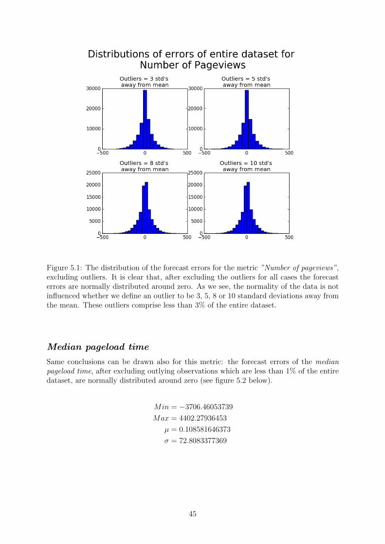
Figure 5.1: The distribution of the forecast errors for the metric ”Number of pageviews”,excluding outliers. It is clear that, after excluding the outliers for all cases the forecasterrors are normally distributed around zero. As we see, the normality of the data is notinfluenced whether we define an outlier to be 3, 5, 8 or 10 standard deviations away fromthe mean. These outliers comprise less than 3% of the entire dataset.

Median pageload time

Same conclusions can be drawn also for this metric: the forecast errors of the medianpageload time, after excluding outlying observations which are less than 1% of the entiredataset, are normally distributed around zero (see figure 5.2 below).

Min = −3706.46053739

Max = 4402.27936453

µ = 0.108581646373

σ = 72.8083377369

45

Figure 5.2: For this metric too, the distribution of the forecast errors is normal aroundzero.

One important note here, concerning which errors should be included when presentingthe above histograms, is the following: on chapter 3 when explaining the initializationmethods of Holt-Winters, a method of averaging the observations of the first seasonal cycle- which is the first day or the first week of the dataset, depending on which seasonalitypattern we chose - was explained. For Taylor’s model, initialization (3.12) was also basedon the same reasoning of averaging. It is important here to stress that, the forecastsproduced for the first day or week of Holt-Winters and Taylor’s forecasts for the firstweek when using the initialization (3.12) will produce extremely accurate forecasts, theerrors of which will be extremely low, almost negligible. This will result in a biased-towards-zero mean and in a standard deviation that is in fact higher than this computed.The errors of these period are thus not representative and should be excluded whentesting their normality.

The next and final step, after defining a measure of deviation between the expectedand observed behaviour, is a rule which decides whether each observation, according tothis deviation is marked as normal or abnormal. This choice is made according to thedistance of the forecast errors from the mean in terms of standard deviations. We seek

46

to define this threshold - the number of σ’s - that makes the most accurate distinctionbetween a normal observation and an anomaly (similarly with the model of Ward et al.[1998]).

5.2 Generating an alarm and evaluating performance

We should not assume that a failure in a website is caused by only one anomalous datapoint of a metric, but instead we should expect that an anomalous behaviour occurswhen for multiple time steps the behaviour observed is not compatible with the expectedbehaviour. Consequently we will use a moving window of consecutive anomalies to bea reason for identifying an abnormal behaviour. A question that naturaly follows andneeds to be answered before all is:

How many consecutive anomalies/outliers should cause the raise of analarm?

This question can also be translated in the business context as follows:

How many time steps (or minutes in our case) is it appropriate forMeasureWorks to inform the website owner company about an anomalous

behaviour?

Of course this number depends on the preference of the company, but also depends onthe dataset. There might be cases where there is information, coming from backgroundknowledge, that an error or failure on a website results after k consecutive abnormalobservations, where k is to be determined. In our case we make the following conventions:

• Individual abnormal observations will be refered to as outliers or anomalous datapoints.

• An alarm is raised, indicating that anomalous behaviour was detected and needsattention, when k = 3 consecutive outliers are detected, or when k = 3 outliers areobserved within 5 minutes. We refer from now on to any succession of 3 or moreoutliers as an anomalous area.

47

Evaluating True/False positives

As we explained in the beginning of chapter 4, the missing values of the dataset were filledin with the average of the preceeding and proceeding observations, a necessary processfor training the model. We did this both on the train and the test set, even though theforecast errors for the replaced missing values of the test set were not considered whencomputing the MAE of each model. For the evaluation of the anomaly detection modelthough, we will use the test set where the missing values were not replaced by the average,but were set equal to zero, for the following reason: since we do not know the reasonthat these values were missing, we could assume that they could be potential anomalies.Treating them as so, will allow us to have more anomalous data points in the test-set forevaluating the performance of our model.

The evaluation of the Gaussian anomaly detector will be done in terms of ”TruePositives” and ”False Positives”. The terms Positive/Negative refers to whether we iden-tified and labelled observations as anomalous or not. Since we are counting anomalies,”Positive” refers to an anomalous and ”Negative” to a normal observation. The termsTrue/False refers to whether our labelling was correct or not (source: Flach [2012]). Thereare then four different possibilities, which in our anomaly detection context will be asfollows:

1. True Positives:Anomalies that correctly were labelled as so. In our context we may refer to themalso as correct detections.

2. False Positives:Anomalies that were wrongly labelled as normal observations. We will refer to themalso as missed detections or missed anomalies.

3. True Negatives:Normal datapoints that were correctly labelled as so.

4. False Negatives:Normal observations that were wrongly labelled as anomalies, which we will fre-quently refer to as false detectons or false alarms.

A good anomaly detection model is the one which maximizes the number of correctdetections while at the same time keeps the number of false detections in as low levels aspossible. Unfortunately in our case, there is no information about which ones among theoutliers are true anomalies or not, a valuable information when selecting which thresholdis the one yielding the most true positives and the less false negatives. In order toevaluate the accuracy of our anomaly detection model we will find the anomalies byvisual inspection from the graphs, and consider them to be actual anomalies, which wewill seek to identify with the Gaussian anomaly detection model. This evaluation will bedone, of course, on the test set.

48

Number of pageviews

On figure 5.6 the actual behaviour of the metric number of pageviews on the test set isplotted. In total 22 anomalous points or anomalous areas were found, as circled withgreen color on figure 5.6. Our objective is to find out how many of these were identifiedby the model. Some of these anomalous areas are abnormal data points for more than3 consecutive minutes. We make the convention that a raise of a single alarm on ananomalous area containing more than 3 consecutive anomalies is considered succesfull.As an example, on the first day of the test set, the 23/5, there is an abnormal behaviourmarked for a couple of hours (first gren circle). The detection will be considered succesfulif at least three consecutive outliers are detected at these area.

Figure 5.3: The green circles indicate the point of appearance of an outlier or the area ofan anomalous behaviour. We use these as ground truth when evaluating the performanceof the anomaly detector. See also figure 15 on the appendix.

We will test four different thresholds: an observation will be defined as anomalous/out-lier when its forecast error has a distance greater than 3, 5, 8 or 10 standard deviationsfrom the mean of the errors. On table 5.2, as well as on figure 5.7 on the next page wesee the results of all the four cases. It seems that the threshold of 3σ detects the mostanomalous areas or outliers compared to the rest. The cost for that though is the highnumber of False Negatives, a value way greater than the remaining thresholds. For thethreshold of 10σ we observe the smallest number of false alarms, though its performanceis notably inferior than the threshold of 3σ.

Threshold Correct detections False detectionserror > 3σ 20/22 587error > 5σ 17/22 60error > 8σ 16/22 29error > 10σ 16/22 5

Table 5.1: Performance of the anomaly detector for 4 different thresholds, for the metricnumber of pageviews. An objective belief is that the threshold of 5σ is balanced betweenthe number of correct detections and false alarms.

49

Figure 5.4: For the four different cases of thresholds chosen, the anomalous points de-tected are marked as red stars. The True Positives are marked as green circles, while theFalse Positives are circled in red color.

50

A closer look on figure (5.5) reveals the reason why the Gaussian anomaly detectorwith threshold 3σ succesfully identifies the presence of more anomalous areas comparedto the other thresholds. These extra detections, the two red circles in the beggining of2/6 and the one in the beggining of 5/6, are taking place in the early morning hoursbetween 1:00am to 6:00am. In these early morning hours where the anomalies occured,the level of the time series data is very low and thus the drop on the number of pageviewsis small enough and is captured only by the - more sensitive in small changes thresholdof - value 3σ.

One way to deal with this problem is to draw not one, but 1440 distributions for theresiduals instead, one for each minute of the day. Then the distributions corresponding tothe minutes for these morning hours would have different standard deviations - smallerin particular - than the rest, making them more sensitive to changes, resulting in thedetection of future errors. We can see that the errors behave differently during the day -smaller errors during the less busy hours and greater errors during the busy hours - whenplotting the forecast errors for the test set, shown in figure 15.

On the other hand, one of the drawbacks of this method is that, we would need atleast 30 days of data before we could compute the mean and standard deviation of eachof these 1440 normal distributions. As stated by David M. Diez [2012], the populationstandard deviation can reasonably be substituted by the sample standard deviation whenthe sample size is at least n = 30. An alternative to that could be to draw 2 differentdistributions, one for the busy hours where the errors are higher and one for the less busyhours, in which the forecast errors fluctuate in lower levels, or even use a classificationmethod to define this number of different normal distributions.

Figure 5.5: The forecast errors for the test set for the metric ”Number of pageviews”, forthe two best performing models: Taylor’s DS additive and Holt-Winter’s with additivedaily seasonality.

51

Median pageload time

Since the behaviour of the metric Median pageload time is different than the one of numberof pageviews, different thresholds will be used. For this metric, due to higher variability,we choose lower thresholds, mainly 5, 6, 7 and 8 standard deviations away from the meanof the forecast errors.

Figure 5.6: The green circles indicate the point of appearance of an outlier or the area ofan anomalous behaviour. We use these as grand truth when evaluating the performanceof the anomaly detector. See also figure 15 on the appendix.

Threshold Correct detections False detectionserror > 5σ 20/20 82error > 6σ 19/20 28error > 7σ 19/20 15error > 8σ 18/20 4

Table 5.2: Performance of the anomaly detector for 4 different thresholds, for the met-ric median pageload time. For both metrics the number of correct outliers detected isconsidered instead of the number of correct alarms raised.

52

Figure 5.7: For the four different cases of thresholds chosen, the anomalous points de-tected are marked as red stars. Again the True Positives are marked as green circles,while the False Positives are circled in red color.

53

5.3 Building robust forecasting models using the Gaus-

sian anomaly detector

In the previous chapter we presented the results when all forecasting models to be testedwere applied on the initial dataset where outliers were not treated differently than theother data points, only the missing vaues were filled in with an average, due to theinability of the models to treat missing values. In this section we will talk about theinfluence of outliers in the forecast accuracy.

In his paper, [Goodwin, 2010] notes three important weaknesses of Holt-Winter’smethod for forecasting. One of these weaknesses, which is of greatest importance inour context, is the impact of outliers on the forecasts. Similarly, Gelper et al. [2010]remark that, even though the superiority and competitiveness of Holt-Winters’ methodcompared to other more complicated forecast methods, its performance is considerablydeteriorating in the presence of outliers. As a variation and extension of Holt-Winters,the same problem applies also to Taylor’s double seasonal model.

Remember from chapter 3 that every forecast can be broken into three components,namely the level, trend and seasonality components, which are updated in every time stepand their values are determined by the observations previously seen. [Goodwin, 2010]claims that unusually high or low values present in the dataset can cause the models tooverestimate or understimate the rates in which the time series is increasing or decreasing,and consequently the value of the forecast of the next period will be too high or too low.

Furthermore, another issue that could arise because of the presence of outliers con-cerns the optimal smoothing parameters. We have seen that the smoothing parametersdetermine how sensitive the model is to the latest observations and a common methodin finding the optimal ones is by identifying the values of the parameters that producethe most accurate forecasts of the past. As [Goodwin, 2010] notes, in the presence ofunusually high or low observations there is the danger that forecasts react too slowly ortoo rapidly, with a consequence of distorting the smoothing parameters.

This topic on how to treat outliers and anomalous observations for improving theforecast accuracy of the models previously explained is intentionally left for this chapter,after the deployment of the anomaly detection model. The reason for that is the factthat, after an anomalous observation is detected by the Gaussian model, a different value,smoother and more ’normal’ is used for determining the values of the level, trend andseasonal components instead. This technique is inspired by the work of Gelper et al.[2010], with the difference that they use robust scale estimators (such as the median ab-solute deviation for example) instead of the standard deviation, which we chose to usefor now due to time limitations. This technique of using the Gaussian anomaly detectornot only to detect an anomaly, but also to replace it with a ’cleaned’ value for improvingthe future forecasts will be implemented to all the forecasting methods examined before,and their performance of the classic version will be compared with the performance ofthe robust one.

54

Comparison between classical and robust models

The evaluation of the forecasting models will be done, of course, on the test set, withone main difference: the time points of the anomalous observations detected will not beincluded in the computation of the MAE. For the instances where an abnormal behaviorwas detected, a good forecast will be the one that actually deviates a lot from the observedabnormal behaviour. A high value of the MAE in these points translates into a predictioncurve that stays robust, without being influenced by the extremelly high or low valuesof the curve of the observed behaviour, while a low value of the MAE for these pointswill mean that the prediction curve closely follows the actuall anomalous behaviour ofthe metric.

Model id Model Classic Version Robust Version1 EWMA 985.78 -2 HW-add(1440) 78.42 72.433 HW-mult(1440) 75.26 71.764 HW-add(10080) 78.31 74.275 HW-mult(10080) 94.16 91.606 Taylor DS-add 71.58 68.507 Taylor DS-mult 72.65 69.33

Table 5.3: The mean absolute error (MAE) computed for the classic and robust versionsof all forecasting models, for the metric ”Number of pageviews”. The threshold 5σ wasused for detecting an anomaly.

Model id Model Classic Version Robust Version1 EWMA 63.65 -2 HW-add(1440) 17.75 15.613 HW-mult(1440) 16.60 15.614 HW-add(10080) 19.04 16.965 HW-mult(10080) 17.75 16.826 Taylor DS-add 15.52 15.047 Taylor DS-mult 16.13 15.68

Table 5.4: Comparison of the MAE for the metric ”Median pageload time” on the testset. For both metrics these performance results were computed without considering thefilled-in missing values with an average, nor the instances that anomalous behaviour wasdetected, in the test set. The dataset was cleanded first 2 distorted last 2, σ = 5

55

From tables 5.3 and 5.4 it is obvious that the robust forms of all the models performbetter than the classic versions. Even though the difference is not significant, whenevaluating in a bigger test set the improvement can be more obvious. In this point wewould like to underline and stress the importance of using these robust forms of thepredictive models, which result in the imporvement of the forecasts, something that isclosely related also to the ability of the anomaly detector to correctly identify anomalies,and avoiding False Positives.

The importance of using the robust versions of the predictive models is more clearlyseen when using Taylor’s model with a different initialization method. Two differentinitialization methods were described in chapter 3 about Taylor’s model: the one, method(3.11), was an arbitrary method setting the starting values of the components equalto zero or one, while method (3.12) used simple averages for producing these startingvalues. From tables 5.5 and 5.6 we see that, even though the improvement in the forecastaccuracy for initialization method (3.11) is not significant, the same does not hold forinitialization method (3.12). For the metric number of pageviews, the robust versionimproves the forecast accuracy by 12% and 15% for Taylor’s additive and multiplicativemodel correspondingly, compared to the classic version.

Initialization method Classic Version Robust Versionarbitrary: (3.11) 71.58 68.50averaging: (3.12) 81.81 71.39

Table 5.5: The MAE computed on the test set, for number of pageviews for the twodifferent initialization methods of Taylor’s DS additive model.

Initialization method Classic Version Robust Versionarbitrary: (3.11) 72.65 69.33averaging: (3.12) 87.33 73.93

Table 5.6: The MAE computed on the test set, for number of pageviews for the twodifferent initialization methods of Taylor’s DS multiplicative model.

According to Taylor [2010b], the success of various optimization algorithms dependsprimarily on the choice of the initial values for the smoothing parameters. From theirside, the optimal smoothing parameters depend to a high extend on the quality of thedata and on the initialization of the forecast models. For the two different initializationmethods, 2 different quadruples of parameters were found, which are presented on theappendix in the end of the documentation. Furthermore, since initialization is influencedby the quality of the data, we manually replaced the outliers of the first two weeks witha more ”normal” value, namely the average of the 4 neighbouring observations.

The reason that initialization method (3.11) yields more accurate results than (3.12)is worth to investigate. It is reasonable to expect

56

We summarize this important conclusion, that the following are interelated and in-fluenced by each other, regarding the class of the Exponential Smoothing forecastingtechniques:

1. the initialization method,

2. the quality of the data,

3. the optimal smoothing parameters,

4. the accuracy of the forecasts.

Computational speed in real time anomaly detection

We need to know the mean and variance of the forecast errors at each minute:The mean of the errors will be

µ =

∑ni=1 ein

The variance will be

σ2 =

∑ni=1(ei − µ)2

n

=

∑ni=1(e

2i − 2 · µ · ei + µ2)

n

=

∑ni=1(e

2i − 2 · µ · ei + µ2)

n

=

∑ni=1 e

2i − 2µ ·

∑ni=1 ei +

∑ni=1 µ

2

n

=

∑ni=1 e

2i

n− 2µ ·

∑ni=1 ein

+n · µ2

n

=

∑ni=1 e

2i

n− 2µ2 + µ2

which gives the following alternative expression for the variance:

σ2 =

∑ni=1 e

2i

n− µ2

Every one minute, when a new observation becomes available, the values of the meanand variance of the forecast errors need to be recomputed. This process can be timeconsuming if every time all previous observations are considered for these computations,especially when the number of observations grows large. We choose instead to use thealternative formula for the variance, presented above, and store only three values, thosethat are needed for the computation of the mean and variance, namely the sum of theerrors, the sum of the squared errors and the number of total observations, we achieve tospeed up the process, as describd in the code below.

The whole process of detecting an anomaly in real time can then be summarized inthe following six steps:

1. Forecast for the next minute is made, denote it by yt+1.

57

2. After one minute has passed, the actual value, yt+1, is made available. The forecasterror is thus computed:

et+1 = yt+1 − yt+1

3. Evaluation of whether the forecast error et+1 - and thus the actual value yt+1 - isconsidered an anomaly is made. This is done by computing how many standard de-viations away from the mean the forecast error et+1 lies. If it exceeds the threshold,then it is labelled as an anomalous observation.

4. The replacement of the ouliers should be done real-time, when the forecasts areproduced: Instead of using this anomalous value for computing the level, trend andseasonal components, a smoother value is chosen, mainly the one lying exactly onthe threshold value.

5. The new mean and variance are computed using the above formulas. The code forthis step will look like this:

# Python code:

sum_of_errors = sum_of_errors + e

sum_of_squared_errors = sum_of_squared_errors + e^2

number_of_observations = number_of_observations + 1

# Using the result of (1):

mean = sum_of_errors / number_of_observations

# Using the result of (2):

variance = (sum_of_squared_errors / number_of_observations) - mean^2

6. Repeat the process from step 1 to step 6 for the next minute.

58

CHAPTER 6

Conclusion

The purpose of this thesis is to build an anomaly detection tool that will identify po-tential downfalls and malfunctions on websites in real time. The problem can be brokendown into three main parts. The first one is the construction of an appropriate modelcapable of being trained on the normal behaviour of our metrics. Due to the multipleseasonal patterns of our metrics, the class of exponential smoothing forecasting models,being capable of dealing with seasonal time series, was chosen, also due to its simplicity,transparency and lower computational demand. From this class, Taylor’s model account-ing for both daily and weekly seasonality patterns was found to outperform Holt-Wintersaccounting for either daily or weekly seasonal effects, in terms of forecasting accuracy.

Secondly, by knowing this normal behaviour, a measure of deviation of each instancefrom this standard behavioural pattern is defined. Due to the numerical character of timeseries, the choice of the forecast error is made. Finally, by observing that these errors arenormally distributed around 0 with an unknown standard deviation of σ, the anomalydetection model is built to flag as anomalies those observations for which their forecasterrors were found to be unexpectedly high or low.

Regarding the true nature of the outliers of our dataset, and if they can be definedas actual anomalies or not, there is not enough information about it. Therefore, theevaluation was conducted by manually setting some outliers as exemplar anomalies andthen by choosing which sigma achieved the most correct detections. According to ourobservations and subjective views on anomalies, for each of the two metrics, the σ’sthat delivered the most balanced results while managing to limit wrong detections, werehighlighted.

By lowering the limitations of the threshold and thus detecting all possible anomalies,the tool will detect a range of false negatives. In this way, the amount of supposedly de-tected anomalies will create doubts about the efficiency of the tool. Conversely, choosingto raise the threshold could result in decreasing the quantity of detected anomalies butalso preventing the tool from identifying true positives.

Judging from the aforementioned choices regarding the detection tool, the clients andtheir needs are the ones that will decide if they prefer capturing all the anomalies orjust the most important ones. Furthermore, it is them who are to determine how manyconsecutive anomalies should lead to the raise an alarm. To conclude, despite the building

59

process of an anomaly detector, there will always be other questions to be viewed andanswered from the perspective of the clients. A modeler-client relationship is reciprocaland thus exchanging views and insights can lead to optimization of the offered services.

6.1 Further work

The further research can be centered around the maintenance and functionality of theanomaly detector in real time in the future. However, these possible improvements do notconcern only anomaly detection related issues but also research ideas that will improveMeasureWork’s scope as a company.

1. Assuming the existence of common sub-cycles of weekdays

Regarding Holt-Winters method accounting for seasonality of length m, the seasonalcomponents s1, s2, ..., sm are updated only once during one seasonal cycle, i.e. once everym time periods. Similarly, in Taylor’s model considering daily and weekly seasonalitypatterns with seasonality cycles of length m1 and m2, the daily seasonal componentsD1, D2, ..., Dm1 are updated only once every day while the weekly seasonal componentsW1,W2, ...,Wm2 are updated only once per week. The models consequently fail to considerthe seasonal changes between one day and the next, since the seasonal variation of a timeinstant for a specific day of the week is computed according to the same time instant of thesame week day of the previous week. Any relevant information between two consecutivedays of the week is not taken into account.

Furthermore, Taylor’s double seasonal model would require 1 initial value for the level,one for the trend, m1 for the daily seasonal and m2 for the weekly seasonal components,meaning that the model would need estimates of m1 + m2 + 2 values before it startsoperating. However, recall from the exploratory data analysis of Chapter 2, our findingregarding the metric Number of pageviews that its behaviour follows the same intra-day cycle from Mondays to Thursdays, and Fridays, Saturdays, and Sundays all form adistinct category in terms of their intra-day behaviour.

In their paper, Gould et al. describe a method of taking advantage of the commonsubcycles and thus reducing the number of seed values the models require. In our case,instead of assuming 7 distinct subcycles, each one for a different day of the week, wecould instead use 4 subcycles, reducing the number of seed values for the seasonal termsneeded from m1 + m2 = 1440 + 7 · 1440 = 11520 to m1 + m2 = 1440 + 4 · 1440 = 7200,by reducing the number of daily cycles from k = 7 to k = 4.

This model for multiple seasonal processes (MS) as it is named by Gould et al., alsoallows for each day to have its own hourly pattern or to have some days with the samepattern. In addition to that, this model allows days with different patterns to affect oneanother, overcoming the weakness of Taylor’s double seasonal model, which assumes thesame intra-day cycle for all days of the week. By considering different daily cycles foreach seperate day of the week - or categorizing them in groups according to behaviouralsimilarity - and by treating the public holidays or special days as Sundays Gould et al.succeed on reducing the mean squarred forecast error by 15% compared to the Holt-Winters with either daily or weekly seasonality or to Taylor’s double seasonal model.Same practice is also followed by Taylor [2010a] with his Intra day exponential smoothingmethod or IC exp smoothing as he names it.

60

2. Recomputation of the smoothing parameters

According to Taylor [2010b], the success of various optimization algorithms dependsprimarily on the choice of the initial values for the smoothing parameters. From their side,the optimal smoothing parameters depend to a high extend on the quality of the data andon the initialization of the forecast models. A further improvement in the maintenanceof the forecasting models would be to use an adaptive Holt-Winters or Taylor’s modelfollowing the suggestion of Kalekar [2004]. This mainly means that the parameters α, βand γ would be recomputed after some period of time. This way the model adapts itselfto the changes. The newly computed parameters may be computed either using the kmost recent data, either all the available data from the start till the current point of time.In the latter case all past data need to have been stored.

3. Holiday effects

Holiday effects are responsible for changes in the behaviour of the data. From the plots ofChapter 2 we have seen that the national Dutch holidays have a different daily pattern,without this declination from the expected pattern to mean that there is an abnormalbehavior. For that reason, in order to avoid false alarms, accounting for special daysand holidays is a necessity. In the paper of Souza et al. [2007] a rule to correct theforecasting of electricity demand on holidays or special days was proposed. This methodto account for holiday effects by applying exogenous corrections produced a considerableimprovement in the forecasting accuracy.

4. Different forecast horizons

In the current research we chose to only consider and investigate performance and com-parison of the forecasting models for the case where we forecast h = 1 minute ahead inthe future. It would be interesting to investigate the effect of longer forecast horizonsin model selection and model performance, and define the h yielding the most accu-rate forecasts. Even though, as we explained in previous chapter, for the procedure ofanomaly detection there is no reason of forecasting longer than 1 minute ahead, it wouldbe valuable for MeasureWorks to present predictions further than one minute ahead inits dashboard.

61

Appendices

62

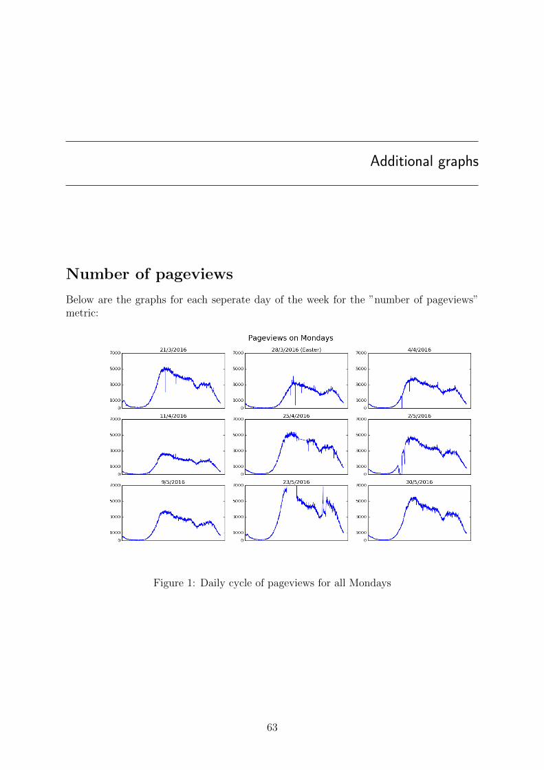
Additional graphs

Number of pageviews

Below are the graphs for each seperate day of the week for the ”number of pageviews”metric:

Figure 1: Daily cycle of pageviews for all Mondays

63

Figure 2: Daily cycle of pageviews for all Tuesdays

Figure 3: Daily cycle of pageviews for all Wednesdays

64

Figure 4: Daily cycle of pageviews for all Thursdays

Figure 5: Daily cycle of pageviews for all Fridays

65

Figure 6: Daily cycle of pageviews for all Sarurdays

Figure 7: Daily cycle of pageviews for all Sundays

66

67

68

69

70

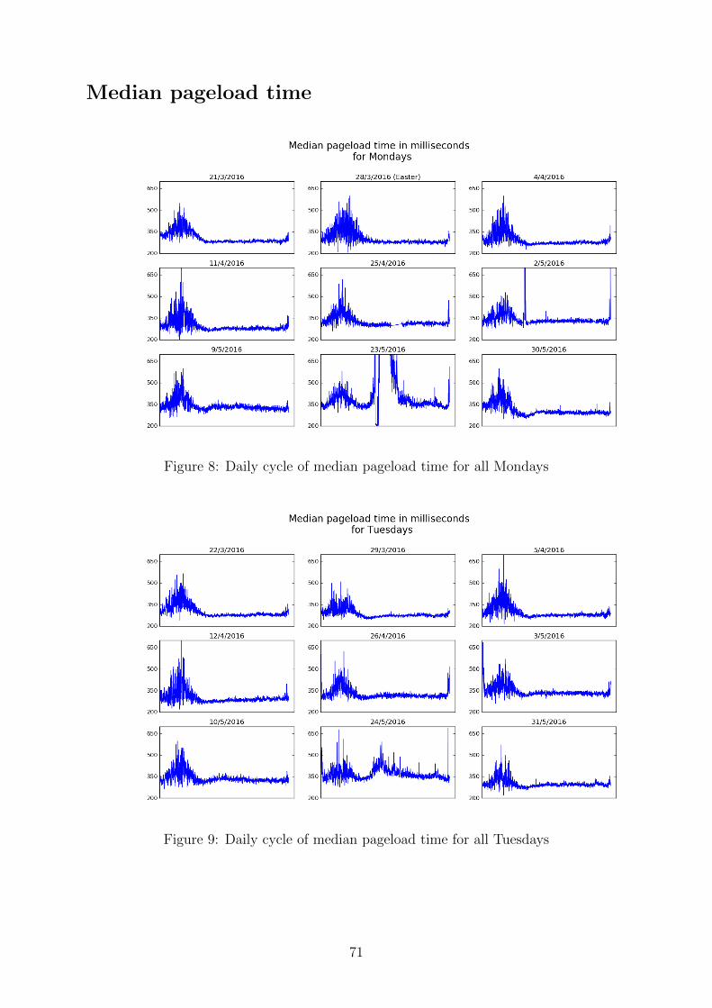
Median pageload time

Figure 8: Daily cycle of median pageload time for all Mondays

Figure 9: Daily cycle of median pageload time for all Tuesdays

71

Figure 10: Daily cycle of median pageload time for all Wednesdays

Figure 11: Daily cycle of median pageload time for all Thursdays

72

Figure 12: Daily cycle of median pageload time for all Fridays

Figure 13: Daily cycle of median pageload time for all Saturdays

73

Figure 14: Daily cycle of median pageload time for all Sundays

74

Figure 15: The anomalies we mark on the test set, 22 anomalous ”areas” in total.

75

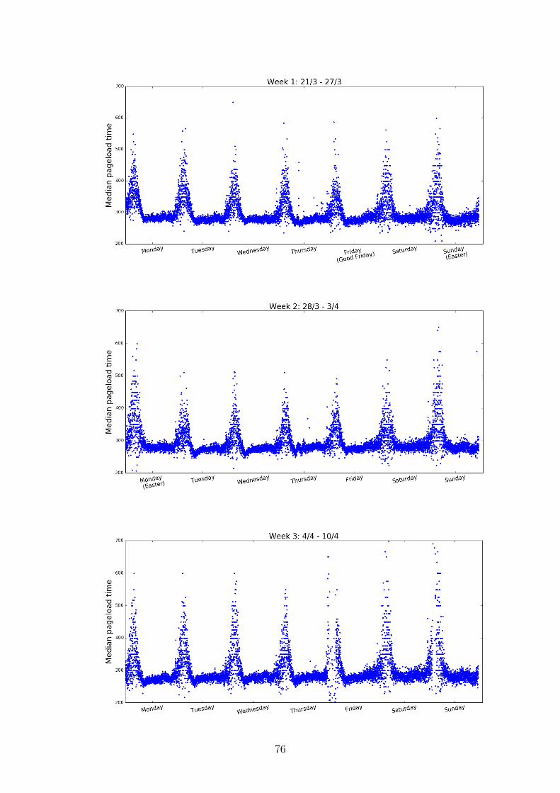
76

77

78

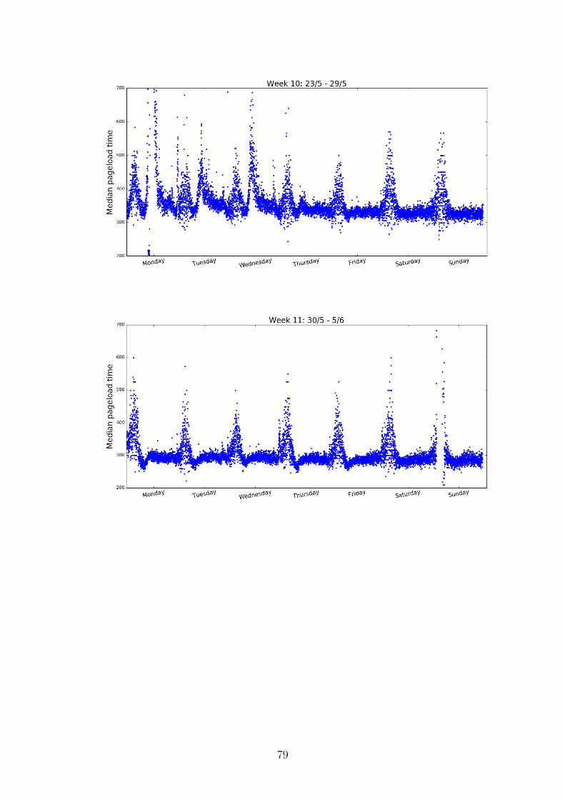
79

Tables for the smoothing parameters

Here we present analytically all the optimal smoothing parameters found for all themodels and different cases:

Holt-Winters: ”Number of pageviews”

Daily

Additive MAE train = 67.208α = 0.310344827586

β = 0γ = 0.137931034483

Multiplicative MAE train = 71.26α = 0.206896551724

β = 0γ = 0.0689655172414

Weekly

Additive MAE train = 64.74α = 0.241379310345

β = 0γ = 0.310344827586

Multiplicative MAE train = 72.018α = 0.0698965517241

β = 0γ = 0.0354482758621

Table 1: Optimal parameters found for the metric ”Number of Pageviews” for the Clas-sical Holt-Winters model. The MAE is computed on the train set and the number ofparameter combinations explored is 303. (checked, correct)

80

Holt-Winters: ”Median pageload time”

Daily

Additive MAE train = 20.61α = 0.275862068966

β = 0γ = 0.0344827586207

Multiplicative MAE train = 20.21α = 0.275862068966

β = 0γ = 0.0689655172414

Weekly

Additive MAE train = 20.34α = 0.275862068966

β = 0γ = 0.172413793103

Multiplicative MAE train = 20.32α = 0.275862068966

β = 0γ = 0.206896551724

Table 2: Optimal parameters found for the metric ”Median pageload time” for the Clas-sical Holt-Winters model. The MAE is computed on the train set and the number ofcombinations of the parameters explored is 303. (checked, correct)

81

Taylor’s DS, (3.11) initialization method

Number of pageviews

Additive MAE train = 61.15α = 0.25β = 0.0416γ = 0δ = 0

Multiplicative MAE train = 61.707α = 0.214857142857β = 0.0722857142857

γ = 0δ = 0

Median pageload time

Additive MAE train = 19.16α = 0.263157894737

β = 0γ = 0δ = 0

Multiplicative MAE train = 19.556α = 0.368421052632

β = 0γ = 0δ = 0

Table 3: Optimal parameters found for the two metrics for Taylor’s DS model using theinitialization method (3.11). The number of parameter combinations explored was 254

for the Number of pageviews and 204 for the Median pageload time.

82

Taylor’s DS, (3.12) initialization method

Number of pageviews

Additive MAE train = 65.22α = 0.210526315789

β = 0γ = 0

δ = 0.263157894737

Multiplicative MAE train = 62.679α = 0.157894736842

β = 0γ = 0

δ = 0.157894736842

Median pageload time

Additive MAE train = 19.989α = 0.263157894737

β = 0γ = 0

δ = 0.105263157895

Multiplicative MAE train = 20.26α = 0.263157894737

β = 0γ = 0

δ = 0.210526315789

Table 4: Optimal parameters found for the two metrics for Taylor’s DS model,using theinitialization method (3.12). The number of parameter combinations explored was 204

for both metrics.

83

Bibliography

S Tom Au, Guang-Qin Ma, and Shu-Ngai Yeung. Automatic forecasting of double sea-sonal time series with applications on mobility network traffic prediction. In 2011 JointStatistical Meetings, July, 2011.

Peter J. Brockwell and Richard A. Davis. Introduction to Time Series and Forecasting,chapter 9. Springer, 2010.

Jake D Brutlag. Aberrant behavior detection in time series for network monitoring. InLISA, volume 14, pages 139–146, 2000.

Paulo Cortez, Miguel Rio, Miguel Rocha, and Pedro Sousa. Multi-scale internet trafficforecasting using neural networks and time series methods. Expert Systems, 29(2):143–155, 2012.

Mine Cetinkaya-Rundel David M. Diez, Christopher D. Barr. OpenIntro Statistics, chap-ter 4: Foundations for Inference. CreateSpace Independent Publishing Platform, 2ndedition, 2012.

Ted Dunning and Ellen Friedman. Practical Machine Learning: A new look at anomalydetection. O’Reilly Media, 1st edition, 2014.

Peter Flach. Machine Learning: the art and science of algorithms that make sense ofdata. Cambridge University Press, 1st edition, 2012.

Sarah Gelper, Roland Fried, and Christophe Croux. Robust forecasting with exponentialand holt–winters smoothing. Journal of forecasting, 29(3):285–300, 2010.

Paul Goodwin. The holt-winters approach to exponential smoothing: 50 years old andgoing strong. ResearchGate, 2010.

Rohitha Goonatilake, Susantha Herath, and Ajantha Herath. Probabilistic models foranomaly detection based on usage of network traffic. Journal of Information Engineer-ing and Applications, 3(9):28–40, 2013.

Phillip G Gould, Anne B Koehler, Farshid Vahid-Araghi, Ralph D Snyder, J Keith Ord,and Rob J Hyndman. Forecasting time-series with multiple seasonal patterns.

84

Rob J Hyndman. Measuring forecast accuracy. 2014.

Rob J Hyndman and George Athanasopoulos. Forecasting: principles and practice, chap-ter 7: Exponential smoothing. OTexts, 2013.

Rob J Hyndman and Anne B Koehler. Another look at measures of forecast accuracy.International journal of forecasting, 22(4):679–688, 2006.

Rob J Hyndman, Anne B Koehler, Ralph D Snyder, and Simone Grose. A state spaceframework for automatic forecasting using exponential smoothing methods. Interna-tional Journal of Forecasting, 18(3):439–454, 2002a.

Rob J Hyndman, Anne B Koehler, Ralph D Snyder, and Simone Grose. A state spaceframework for automatic forecasting using exponential smoothing methods. Interna-tional Journal of Forecasting, 18(3):439–454, 2002b.

Nur Adilah Abd Jalil, Maizah Hura Ahmad, and Norizan Mohamed. Electricity loaddemand forecasting using exponential smoothing methods. World Applied SciencesJournal, 22(11):1540–1543, 2013.

Prajakta S Kalekar. Time series forecasting using holt-winters exponential smoothing.Kanwal Rekhi School of Information Technology, 4329008:1–13, 2004.

Spyros Makridakis and Michele Hibon. The m3-competition: results, conclusions andimplications. International Journal of Forecasting, 16:451–476, 2000.

Wes McKinney. Python for Data Analysis. O’Reilly Media, 1st edition, 2012.

Gerhard Munz and Georg Carle. Application of forecasting techniques and control chartsfor traffic anomaly detection. In Proc. 19th ITC Specialist Seminar on Network Usageand Traffic, Berlin, Germany, 2008.

E Monteiro Pena, M de Assis, and M Lemes Proenca. Anomaly detection using forecastingmethods arima and hwds. In proceeding of XXXII International Conference of TheChilean Computer Science Society (SCCC), 2013.

Mihir Rajopadhye, Mounir Ben Ghalia, Paul P Wang, Timothy Baker, and Craig VEister. Forecasting uncertain hotel room demand. Information sciences, 132(1):1–11,2001.

Spyros G. Makridakis Rob J Hyndman and Steven C. Wheelwright. Forecasting: methodsand applications, chapter 4: Exponential smoothing methods. Willie, 3rd edition, 1997.

Vasilios A Siris and Fotini Papagalou. Application of anomaly detection algorithmsfor detecting syn flooding attacks. In Global Telecommunications Conference, 2004.GLOBECOM’04. IEEE, volume 4, pages 2050–2054. IEEE, 2004.

Reinaldo Castro Souza, Monica Barros, and CVC Miranda. Short term load forecastingusing double seasonal exponential smoothing and interventions to account for holidaysand temperature effects. TLAIO II-2 do Taller Latino Iberoamericano de Investigacionde Operaciones. Acapulco, Mexico, pages 1–8, 2007.

85

Maciej Szmit and Anna Szmit. Usage of modified holt-winters method in the anomalydetection of network traffic: Case studies. Journal of Computer Networks and Com-munications, 2012, 2012.

Maciej Szmit, Slawomir Adamus, Sebastian Bugala, and Anna Szmit. Implementation ofbrutlag’s algorithm in anomaly detection 3.0. In FedCSIS, pages 685–691, 2012.

James W Taylor. Short-term electricity demand forecasting using double seasonal expo-nential smoothing. Journal of the Operational Research Society, 54(8):799–805, 2003.

James W Taylor. An evaluation of methods for very short-term load forecasting usingminute-by-minute british data. International Journal of Forecasting, 24:645–658, 2008.

James W Taylor. Exponentially weighted methods for forecasting intraday time serieswith multiple seasonal cycles. International Journal of Forecasting, 26(4):627–646,2010a.

James W Taylor. Triple seasonal methods for short-term electricity demand forecasting.European Journal of Operational Research, 204(1):139–152, 2010b.

Amy Ward, Peter Glynn, and Kathy Richardson. Internet service performance failuredetection. ACM SIGMETRICS Performance Evaluation Review, 26(3):38–43, 1998.

Li Wei, Nitin Kumar, Venkata Nishanth Lolla, Eamonn J Keogh, Stefano Lonardi, andChotirat (Ann) Ratanamahatana. Assumption-free anomaly detection in time series.In SSDBM, volume 5, pages 237–242, 2005.

Nong Ye, Qiang Chen, and Connie M Borror. Ewma forecast of normal system activityfor computer intrusion detection. Reliability, IEEE Transactions on, 53(4):557–566,2004.

86