STATISTICAL MODELING FOR ANOMALY DETECTION, · PDF fileSTATISTICAL MODELING FOR ANOMALY DETECTION, FORECASTING AND ROOT CAUSE ANALYSIS OF ENERGY ... is the IBM Building Energy

STATISTICAL MODELING FOR ANOMALY DETECTION, FORECASTING AND ROOTCAUSE ANALYSIS OF ENERGY CONSUMPTION FOR A PORTFOLIO OF BUILDINGS

Fei Liu1, Young M. Lee1, Huijing Jiang1, Jane Snowdon1, Michael Bobker2

1IBM Thomas J. Watson Research Center, Yorktown Heights, NY, U.S.A.2Building Performance Lab, CUNY Institute for Urban Systems, New York, NY, U.S.A.

ABSTRACTA multi-step statistical analysis procedure is devel-oped to assess energy consumption and to iden-tify energy saving opportunities for large portfo-lios of buildings such as the New York City’s publicschool buildings. The method borrows strengthfrom and makes integrated use of the VariableBase Degree Day (VBDD) regression model, multi-variate regression model and the Auto RegressiveIntegrated Moving Average (ARIMA) model. Theanalytical method provides useful informationto compute energy performance metrics, detectanomaly, forecast and analyze root causes of theenergy consumptions of the buildings, and helpsbuilding facility engineers and property managersto achieve significant energy savings, greenhousegas emission reductions and cost savings.

INTRODUCTIONSaving energy, improving efficiency of energy con-sumption, lowering energy cost, and reducinggreenhouse gas (GHG) emissions are key initia-tives in many cities, municipalities and for build-ing owners and operators. According to the WorldBusiness Council for Sustainable Development,buildings account for 40% of the worlds total en-ergy consumption and, in 2005, nine gigatonsof global carbon dioxide (CO2) emissions, wellahead of transportation and industry (WBCDS,2009; DOE, 2008a). In the United States alone,commercial and residential buildings account for38% of all CO2 emissions and 72% of electricityconsumption according to the U. S. Departmentof Energy (DOE, 2008b,c). Much of the energyconsumption by commercial buildings is spent onlighting (twenty-six percent), followed by heatingand cooling (thirteen percent and fourteen per-cent, respectively) (DOE, 2007).A good example of the energy saving initiatives isthe New York City (NYC)’s PlaNYC (IPCC, 2007;PLANYC, 2007), which aims to reduce the citygovernment’s energy consumption and CO2 emis-sions by 30% by 2030 from 2005 levels. New YorkCity’s government spends over 1 billion a yearon energy on their approximately 4, 000 buildings(e.g. public schools, prisons, court houses, admin-istrative buildings, waste water treatment plants,etc.). NYC plans to invest, each year, an amountequal to 10% of its energy expenses in energy-

saving measures over the next 10 years. Thelargest segment of NYC government buildings arethe 1,400 K-12 public schools, serving 1.1 millionstudents and covering about 150 million squarefeet. The New York City Department of Educationwas interested in understanding how energy effi-cient their buildings are, what factors contributeto inefficiencies, what are the opportunities forimprovement given budget constraints, and howand how much can they contribute to saving en-ergy and reducing GHG emissions toward NYC’sPlaNYC initiative. Developed along the initiativesis the IBM Building Energy and Emission analytics(i-BEETM) Toolset, a new analytical tool which as-sesses, benchmarks, diagnoses, tracks, forecasts,simulates and optimizes energy consumption inbuilding portfolios. Our focus in this paper is thestatistical methodology in i-BEETM, which is de-veloped for detecting anomalies, forecasting androot cause analysis of monthly electricity, gas andsteam consumption.The problem of analyzing and monitoring build-ing energy performance is a key step to improveenergy efficiency and to reduce environmental im-pact and cost. As an initial effort of this initiative,IBM collaborates with the City University of NewYork (IBM, 2011) to analyze the energy use in theportfolio of K-12 public school buildings in NewYork City. We use this building portfolio as ourtest bed example in this paper. The building port-folio consists of about 1, 400 public school build-ings, covering 150 million square feet. In addition,we collect relevant information such as weather,energy and building characteristics. Our objectiveis to develop a statistical methodology to help un-derstand the energy use patterns throughout theschool portfolio.We develop a multi-step statistical analysis proce-dure, which combines the multivariate regressionmodel, the Variable Base Degree Day (VBDD) re-gression model (Kissock et al., 2003) and the AutoRegressive Integrated Moving Average (ARIMA)model, to assess energy use and identify energysaving opportunities for large portfolios of build-ings. In the first step, we build a regression modelwhich correlates the energy consumption withbuilding characteristics. The energy related build-ing characteristics are then identified through thestepwise variable selection technique. The re-

Proceedings of Building Simulation 2011: 12th Conference of International Building Performance Simulation Association, Sydney, 14-16 November.

- 2530 -

sults are valuable in providing building energyperformance scores for the whole portfolio. Ad-ditionally, it offers insights for the energy con-sumption level of new buildings. In the secondstep, to accommodate building heterogeneity, webuild VBDD regression models separately for eachbuilding. These models are used to separate thebase load energy consumption from the weatherdependent usage. The base load separated in-cludes energy consumption related to lighting,which is one of the largest source of consump-tion in commercial building, as well as hot water,cooking and other plug loads such as appliancesand computers. The results in this step consist ofthe base temperature estimates, as well as the esti-mated coefficients for HDD and CDD for all build-ings. In the third step, we further conduct rootcause analysis, by building the multivariate re-gression models for the results from VBDD model,from which the performance scores can be derivedfor base load, heating, and cooling. The VBDDregression model is a popular approach to ana-lyze energy consumption, which assumes an inde-pendent error structure for the regression model.The assumption may not be realistic in practicebecause serial correlations exist for building en-ergy time series data, especially for our applica-tion with a large portfolio of buildings. To over-come this shortcoming, in the last step, we modelthe dependent error structure through the ARIMAmodel. It is possible that behavior of building ten-ants which cannot be captured in the base load,heating load and cooling load in the VBDD modelcan be captured by the ARIMA model. We alsoinclude seasonal factors in the model. From ourexperience, the VBDD model, combined with theARIMA model for the error structure, typicallyprovides improved statistical performance com-pared to using VBDD alone. The results are usedfor detecting abnormal energy use and forecastingenergy consumption for a portfolio of buildings.The proposed technique provides an integratedanalysis for building heterogeneity, the weatherdependent patterns and the temporal dependentpatterns. It has wide applicability in performancemetrics calculation, anomaly detection, forecast-ing and root cause analysis for building energyportfolios. In the remainder of this paper, we willfirst describe the general modeling framework,followed by the application of using the test bedexample of the NYC school building portfolio.

DEVELOPING THE STATISTICAL TOOLKITTo motivate the approach we take to model en-ergy use of building portfolios, it is useful to be-gin at the end, and consider the type of outputsthat will result from the methodology. From thestatistical toolset to be developed, we wanted to

be able to answer the following questions:1. Which building parametric data (e.g., build-

ing characteristics, operational activities andoccupant behavior) is most useful for predict-ing building energy use?

2. How can we benchmark the relative buildingenergy performance within the portfolio?

3. What percentages of the total energy use aredue to base load, heating use and cooling use,respectively?

4. What are the potential improvement oppor-tunities / root causes for less efficient build-ings?

5. How can we offset the weather dependentfactors, and perform improvement trackingand energy savings from retrofit activities?

6. How can we detect abnormal energy use inthe historical energy use data?

7. How much energy do we expect to use in thefuture?

To address these questions, we develop a multi-step statistical modeling strategy. The statisti-cal models utilize typical data collected about thebuilding energy portfolio, such as,

• energy use data for each building;• building characteristics such as the gross

floor area (GFA), age of the building, occu-pant density, and number of each equipmenttype (e.g., refrigerator, freezers, etc);

• building operation and activity;• weather data such as outside temperature

and relative humidity.The statistical modeling strategy we developedconsists of the following three major modules:

• Variable Based Degree Day (VBDD) modelwith building effect for each building;

• Multivariate regression models (Multi-regress): one for the overall energy use ofthe whole portfolio, and ones for base load,heating, cooling which utilize the outputsfrom VBDD of each building;

• Time series models (TS-model), which utilizethe outputs from VBDD.

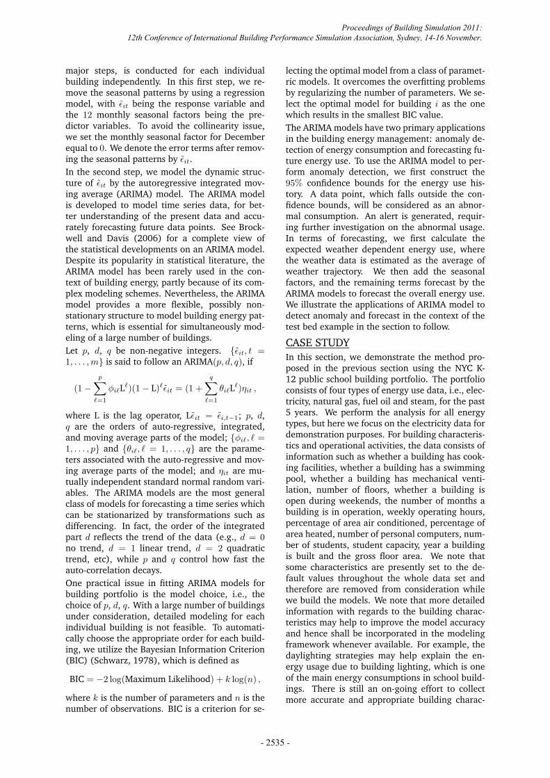
The system is best described by the schematicgiven in Figure 1. We will discuss the modelingdetails in the rest of this section. We note thatthese three modules can be integrated, in order toanswer the aforementioned questions, as follows.

• Multi-regress module is used to answer ques-tions 1, 2.

• VBDD module is used to answer questions 3,5.

• VBDD module and Multi-regress module arecombined together to answer question 4.

• VBDD module and TS-model module are com-


- 2531 -

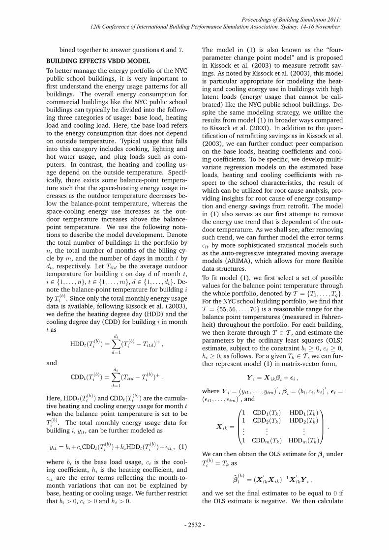
bined together to answer questions 6 and 7.

BUILDING EFFECTS VBDD MODELTo better manage the energy portfolio of the NYCpublic school buildings, it is very important tofirst understand the energy usage patterns for allbuildings. The overall energy consumption forcommercial buildings like the NYC public schoolbuildings can typically be divided into the follow-ing three categories of usage: base load, heatingload and cooling load. Here, the base load refersto the energy consumption that does not dependon outside temperature. Typical usage that fallsinto this category includes cooking, lighting andhot water usage, and plug loads such as com-puters. In contrast, the heating and cooling us-age depend on the outside temperature. Specif-ically, there exists some balance-point tempera-ture such that the space-heating energy usage in-creases as the outdoor temperature decreases be-low the balance-point temperature, whereas thespace-cooling energy use increases as the out-door temperature increases above the balance-point temperature. We use the following nota-tions to describe the model development. Denotethe total number of buildings in the portfolio byn, the total number of months of the billing cy-cle by m, and the number of days in month t bydt, respectively. Let Titd be the average outdoortemperature for building i on day d of month t,i ∈ {1, . . . , n}, t ∈ {1, . . . ,m}, d ∈ {1, . . . , dt}. De-note the balance-point temperature for building i

by T (b)i . Since only the total monthly energy usage

data is available, following Kissock et al. (2003),we define the heating degree day (HDD) and thecooling degree day (CDD) for building i in montht as

HDDt(T(b)i ) =

dt�

d=1

(T (b)i − Titd)+ ,

and

CDDt(T(b)i ) =

dt�

d=1

(Titd − T (b)i )+ .

Here, HDDt(T(b)i ) and CDDt(T

(b)i ) are the cumula-

tive heating and cooling energy usage for month twhen the balance point temperature is set to beT (b)

i . The total monthly energy usage data forbuilding i, yit, can be further modeled as

yit = bi +ciCDDt(T(b)i )+hiHDDt(T

(b)i )+�it , (1)

where bi is the base load usage, ci is the cool-ing coefficient, hi is the heating coefficient, and�it are the error terms reflecting the month-to-month variations that can not be explained bybase, heating or cooling usage. We further restrictthat bi > 0, ci > 0 and hi > 0.

The model in (1) is also known as the “four-parameter change point model” and is proposedin Kissock et al. (2003) to measure retrofit sav-ings. As noted by Kissock et al. (2003), this modelis particular appropriate for modeling the heat-ing and cooling energy use in buildings with highlatent loads (energy usage that cannot be cali-brated) like the NYC public school buildings. De-spite the same modeling strategy, we utilize theresults from model (1) in broader ways comparedto Kissock et al. (2003). In addition to the quan-tification of retrofitting savings as in Kissock et al.(2003), we can further conduct peer comparisonon the base loads, heating coefficients and cool-ing coefficients. To be specific, we develop multi-variate regression models on the estimated baseloads, heating and cooling coefficients with re-spect to the school characteristics, the result ofwhich can be utilized for root cause analysis, pro-viding insights for root cause of energy consump-tion and energy savings from retrofit. The modelin (1) also serves as our first attempt to removethe energy use trend that is dependent of the out-door temperature. As we shall see, after removingsuch trend, we can further model the error terms�it by more sophisticated statistical models suchas the auto-regressive integrated moving averagemodels (ARIMA), which allows for more flexibledata structures.To fit model (1), we first select a set of possiblevalues for the balance point temperature throughthe whole portfolio, denoted by T = {T1, . . . , Tq}.For the NYC school building portfolio, we find thatT = {55, 56, . . . , 70} is a reasonable range for thebalance point temperatures (measured in Fahren-heit) throughout the portfolio. For each building,we then iterate through T ∈ T , and estimate theparameters by the ordinary least squares (OLS)estimate, subject to the constraint bi ≥ 0, ci ≥ 0,hi ≥ 0, as follows. For a given Tk ∈ T , we can fur-ther represent model (1) in matrix-vector form,

Y i = Xikβi + �i ,

where Y i = (yi1, . . . , yim)�, βi = (bi, ci, hi)

�, �i =

(�i1, . . . , �im)�, and

Xik =

1 CDD1(Tk) HDD1(Tk)1 CDD2(Tk) HDD2(Tk)...

......

1 CDDm(Tk) HDDm(Tk)

.

We can then obtain the OLS estimate for βi underT (b)

i = Tk as

�β(k)

i = (X�

ikXik)−1X�

ikY i ,

and we set the final estimates to be equal to 0 ifthe OLS estimate is negative. We then calculate


- 2532 -

© 2010 IBM Corporation IBM Confidential 3

Energy Data •!Electricity •!Gas •!Steam

Building Char •!GFA •!Age •!Occupancy •!Num of Equip

Building Operation

and Activity

Weather •!Temp •!Rel Hum •!Wind •!Solar Rad.

Building Effects VBDD Model

CDD Coef

Base Load

Error

HDD Coef

Bal Temp

Balance temperature

Multivariate Regression

model

Time Series model

Weather forecast

Control bounds

Diagnose root cause

Evaluate Energy efficiency

Perform indicator

Detect anomaly

Forecast future usage

Figure 1: Building energy portfolio analysis system

the R2 under T (b)i = Tk as

R2ik = 1−

�t(yit − y(k)

it )2�t(yit − yi)2

,

where y(k)it is the fitted value for the yit under Tk,

and yi is the sample mean of yit. We hence se-lect the balance point temperature according tothe best fit to the data, i.e., the temperature whichis associated with the largest R2.We summarize the algorithm for fitting model (1)as follows.

Algorithm: Fitting the VBDD model in (1)

• Input: monthly energy usage data yit, i = 1, . . . , nand t ∈ {1, . . . , m}, and outdoor temperature Titd,d ∈ {1, . . . nt}.

• For i ∈ {1, . . . n} and Tk ∈ T ,1. Calculate CDDt and HDDt.2. Estimate bi, ci, hi by OLS, subject to bi > 0,

ci > 0 and hi > 0. Denote the resultantestimates by b(k)

i , c(k)i , h(k)

i .3. Calculate R2

k.4. Select k such that R2

k = maxl∈{1,...,q} R2l ,

and set T (b)i = Tk.

• Output: T (b)i , b(k)

i , c(k)i , h(k)

i , �(k)it , i = 1, . . . , n, t =

1, . . . , m.

MULTIVARIATE REGRESSION MODELSFor large building portfolios like the NYC schoolsystem, the amount of data is usually huge. Withthe energy data being collected cumulatively overtime for each building, a quick overview of the en-ergy performance throughout the portfolio is criti-cal for successful management. The U.S. Environ-

mental Protection Agency (EPA) Energy Star Per-formance Rating EPA (2009) provides a valuablemanagement tool to assess the building energy ef-ficiency, relative to similar buildings and climatezones nationwide. In addition to the nationwidecomparison, the assessment of energy efficiency,relative to peer buildings within the portfolio,which provides local and more detailed informa-tion, is also of great value for the building man-agers. This calls for the development of a “local”performance indicator, solely based on the datawithin the portfolio. In this section, we will de-velop multivariate regression models, which leadto a building performance indicator for local port-folio assessment.We first describe the general method utilized toderive the building performance indicator. Let yi

be the quantity of our interest, typically referredto as the response variable, and xi1, . . . , xip be thep predictor variables. The multivariate regressionmodel takes the form

yi = xi1β1 + xi2β2 + . . . + xipβp + �i , (2)

where β1, . . . βp are the regression coefficients and�i is the error term. As in EPA (2009), we utilizethe multivariate regression model in (2) to nor-malize the response variable according to the pre-dictor variables.In the building portfolio context, the predic-tor variables consist of the building characteris-tics and operational activities, for example, grosssquare feet, number of windows and number ofoperating hours. Some of the predictors are notdirectly energy related. We thus perform a step-wise variable selection procedure, to remove theredundant variables from the model.The multivariate regression model in (2) also


- 2533 -

serves as a reference to the energy use for the gen-eral population in the building portfolio. As a re-sult, while fitting the model, we remove data thatcannot represent the general population (e.g.,outliers). In practice, a data point is identified asan outlier and be removed from the subsequentanalysis if its absolute value of the standardizedresidual is larger than 2. After removing the out-liers, we fit the model again and use the resultantestimates for further analysis.The expected value of the response variable, for aspecific building with given characteristics, can beimmediately calculated as

yi = E(yi | xi1, . . . , xip) = xi1β1+xi2β2+. . .+xipβp .(3)

The standardized residual, zi, can be then calcu-lated as

zi =yi − yi

σ,

where σ is the standard error. We note that fora portfolio with many buildings, the zi approxi-mately follows the standard normal distribution.Matching zi to the standard normal curve, we cancalculate the probability that buildings with thesame characteristics consume more energy thanbuilding i as

P(Z > zi) = 1− Φ(zi) ,

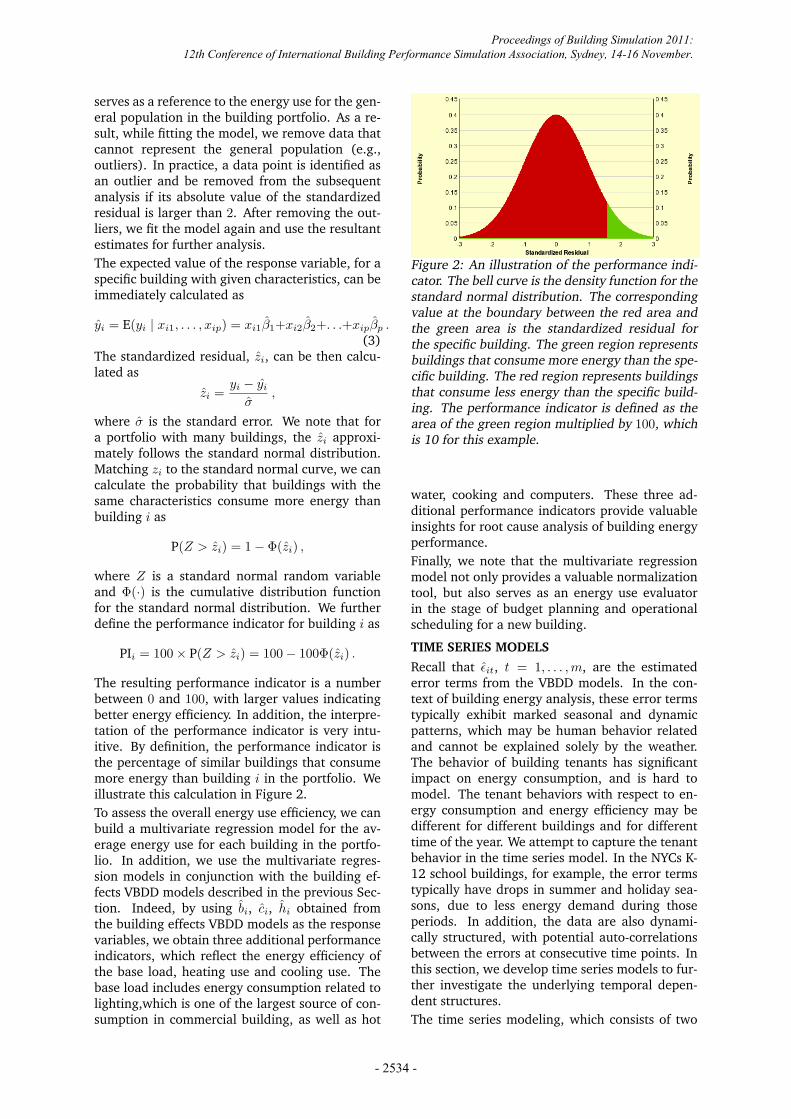
where Z is a standard normal random variableand Φ(·) is the cumulative distribution functionfor the standard normal distribution. We furtherdefine the performance indicator for building i as

PIi = 100× P(Z > zi) = 100− 100Φ(zi) .

The resulting performance indicator is a numberbetween 0 and 100, with larger values indicatingbetter energy efficiency. In addition, the interpre-tation of the performance indicator is very intu-itive. By definition, the performance indicator isthe percentage of similar buildings that consumemore energy than building i in the portfolio. Weillustrate this calculation in Figure 2.To assess the overall energy use efficiency, we canbuild a multivariate regression model for the av-erage energy use for each building in the portfo-lio. In addition, we use the multivariate regres-sion models in conjunction with the building ef-fects VBDD models described in the previous Sec-tion. Indeed, by using bi, ci, hi obtained fromthe building effects VBDD models as the responsevariables, we obtain three additional performanceindicators, which reflect the energy efficiency ofthe base load, heating use and cooling use. Thebase load includes energy consumption related tolighting,which is one of the largest source of con-sumption in commercial building, as well as hot

Figure 2: An illustration of the performance indi-cator. The bell curve is the density function for thestandard normal distribution. The correspondingvalue at the boundary between the red area andthe green area is the standardized residual forthe specific building. The green region representsbuildings that consume more energy than the spe-cific building. The red region represents buildingsthat consume less energy than the specific build-ing. The performance indicator is defined as thearea of the green region multiplied by 100, whichis 10 for this example.

water, cooking and computers. These three ad-ditional performance indicators provide valuableinsights for root cause analysis of building energyperformance.Finally, we note that the multivariate regressionmodel not only provides a valuable normalizationtool, but also serves as an energy use evaluatorin the stage of budget planning and operationalscheduling for a new building.

TIME SERIES MODELSRecall that �it, t = 1, . . . ,m, are the estimatederror terms from the VBDD models. In the con-text of building energy analysis, these error termstypically exhibit marked seasonal and dynamicpatterns, which may be human behavior relatedand cannot be explained solely by the weather.The behavior of building tenants has significantimpact on energy consumption, and is hard tomodel. The tenant behaviors with respect to en-ergy consumption and energy efficiency may bedifferent for different buildings and for differenttime of the year. We attempt to capture the tenantbehavior in the time series model. In the NYCs K-12 school buildings, for example, the error termstypically have drops in summer and holiday sea-sons, due to less energy demand during thoseperiods. In addition, the data are also dynami-cally structured, with potential auto-correlationsbetween the errors at consecutive time points. Inthis section, we develop time series models to fur-ther investigate the underlying temporal depen-dent structures.The time series modeling, which consists of two


- 2534 -

major steps, is conducted for each individualbuilding independently. In this first step, we re-move the seasonal patterns by using a regressionmodel, with �it being the response variable andthe 12 monthly seasonal factors being the pre-dictor variables. To avoid the collinearity issue,we set the monthly seasonal factor for Decemberequal to 0. We denote the error terms after remov-ing the seasonal patterns by �it.In the second step, we model the dynamic struc-ture of �it by the autoregressive integrated mov-ing average (ARIMA) model. The ARIMA modelis developed to model time series data, for bet-ter understanding of the present data and accu-rately forecasting future data points. See Brock-well and Davis (2006) for a complete view ofthe statistical developments on an ARIMA model.Despite its popularity in statistical literature, theARIMA model has been rarely used in the con-text of building energy, partly because of its com-plex modeling schemes. Nevertheless, the ARIMAmodel provides a more flexible, possibly non-stationary structure to model building energy pat-terns, which is essential for simultaneously mod-eling of a large number of buildings.Let p, d, q be non-negative integers. {�it, t =1, . . . ,m} is said to follow an ARIMA(p, d, q), if

(1−p�

�=1

φi�L�)(1− L)��it = (1 +q�

�=1

θi�L�)ηit ,

where L is the lag operator, L�it = �i,t−1; p, d,q are the orders of auto-regressive, integrated,and moving average parts of the model; {φi�, � =1, . . . , p} and {θi�, � = 1, . . . , q} are the parame-ters associated with the auto-regressive and mov-ing average parts of the model; and ηit are mu-tually independent standard normal random vari-ables. The ARIMA models are the most generalclass of models for forecasting a time series whichcan be stationarized by transformations such asdifferencing. In fact, the order of the integratedpart d reflects the trend of the data (e.g., d = 0no trend, d = 1 linear trend, d = 2 quadratictrend, etc), while p and q control how fast theauto-correlation decays.One practical issue in fitting ARIMA models forbuilding portfolio is the model choice, i.e., thechoice of p, d, q. With a large number of buildingsunder consideration, detailed modeling for eachindividual building is not feasible. To automati-cally choose the appropriate order for each build-ing, we utilize the Bayesian Information Criterion(BIC) (Schwarz, 1978), which is defined as

BIC = −2 log(Maximum Likelihood) + k log(n) ,

where k is the number of parameters and n is thenumber of observations. BIC is a criterion for se-

lecting the optimal model from a class of paramet-ric models. It overcomes the overfitting problemsby regularizing the number of parameters. We se-lect the optimal model for building i as the onewhich results in the smallest BIC value.The ARIMA models have two primary applicationsin the building energy management: anomaly de-tection of energy consumption and forecasting fu-ture energy use. To use the ARIMA model to per-form anomaly detection, we first construct the95% confidence bounds for the energy use his-tory. A data point, which falls outside the con-fidence bounds, will be considered as an abnor-mal consumption. An alert is generated, requir-ing further investigation on the abnormal usage.In terms of forecasting, we first calculate theexpected weather dependent energy use, wherethe weather data is estimated as the average ofweather trajectory. We then add the seasonalfactors, and the remaining terms forecast by theARIMA models to forecast the overall energy use.We illustrate the applications of ARIMA model todetect anomaly and forecast in the context of thetest bed example in the section to follow.

CASE STUDYIn this section, we demonstrate the method pro-posed in the previous section using the NYC K-12 public school building portfolio. The portfolioconsists of four types of energy use data, i.e., elec-tricity, natural gas, fuel oil and steam, for the past5 years. We perform the analysis for all energytypes, but here we focus on the electricity data fordemonstration purposes. For building characteris-tics and operational activities, the data consists ofinformation such as whether a building has cook-ing facilities, whether a building has a swimmingpool, whether a building has mechanical venti-lation, number of floors, whether a building isopen during weekends, the number of months abuilding is in operation, weekly operating hours,percentage of area air conditioned, percentage ofarea heated, number of personal computers, num-ber of students, student capacity, year a buildingis built and the gross floor area. We note thatsome characteristics are presently set to the de-fault values throughout the whole data set andtherefore are removed from consideration whilewe build the models. We note that more detailedinformation with regards to the building charac-teristics may help to improve the model accuracyand hence shall be incorporated in the modelingframework whenever available. For example, thedaylighting strategies may help explain the en-ergy usage due to building lighting, which is oneof the main energy consumptions in school build-ings. There is still an on-going effort to collectmore accurate and appropriate building charac-


- 2535 -

teristic data, despite that the process is challeng-ing and time-consuming.Exploratory analysis suggests we take the loga-rithm transformations on the overall energy useand the gross floor area while building the mul-tivariate regression model for the overall energyuse. In addition, to include the building age ef-fects in the model, we note that the building agesare clustered, and we further define the followingfour age factors according to these clusters: (1)prior to 1915 (2) between 1916 and 1945 (3) be-tween 1946 and 1985 (4) after 1986. The step-wise variable selection procedure suggests thatthe gross floor area, percentage of area air condi-tioned, number of students, number of personalcomputers, number of floors, whether a build-ing has cooking facilities, whether a building wasbuilt after 1986 are related to electricity use. Wethus include these variables in the final model. Ac-cording to this model, we can further calculate theoverall energy use efficiency for all buildings inthe portfolio. In Figure 2, we show the buildingperformance indicator for the overall energy usefor a particular building. We refer to this buildingas the demo building. In the rest of this section,we will illustrate the rest results using the demobuilding.We further develop the VBDD models for all build-ings, about 1, 400 buildings, in the portfolio. InTable 1, we show the resultant estimates for bal-ance temperature, base load (kBtu), cooling coef-ficient and heating coefficient for the demo build-ing. We further calculate the cooling energy andthe heating energy used for a particular year usingthe results in this table. Based on these results, wefurther divide the fiscal year energy use into baseload, heating energy use, cooling energy use, andother use.

Table 1: Estimated Base load, cooling coefficientand heating coefficient from the VBDD model forthe demo building. The estimated balance tem-perature is in Fahrenheit and the rest are in theunit of kBtu.

Balance Temperature 60Base Load 521216.90Cooling Coef 153.01Heating Coef 103.88

To conduct the root cause analysis, we build themultivariate regression models for the estimatedbase load, cooling coefficients and heating coeffi-cients from the VBDD models. We can then furtherrank the performance indicators from smallest tothe largest, which corresponds to the retrofit pri-ority for this building. Table 2 shows the perfor-mance indicators for the base load, the heatinguse and the cooling use for the demo building. As

we can see from this table, the demo building hasaverage performance for heating (performance in-dicator equals to 50), below average performancefor base load (performance indicator equals to25), and below average performance for cooling(performance indicator equals to 10). Since thecooling performance is the worst among all threeperspectives, we assign the top priority to retrofitthe cooling system of the building.

Table 2: The performance indicators to analyzethe root cause for the demo building. First col-umn: possible root cause. Second column: perfor-mance indicators. Third column: retrofit priority.

Root Cause PI PriorityBase Load 25 2Cooling 10 1Heating 50 3

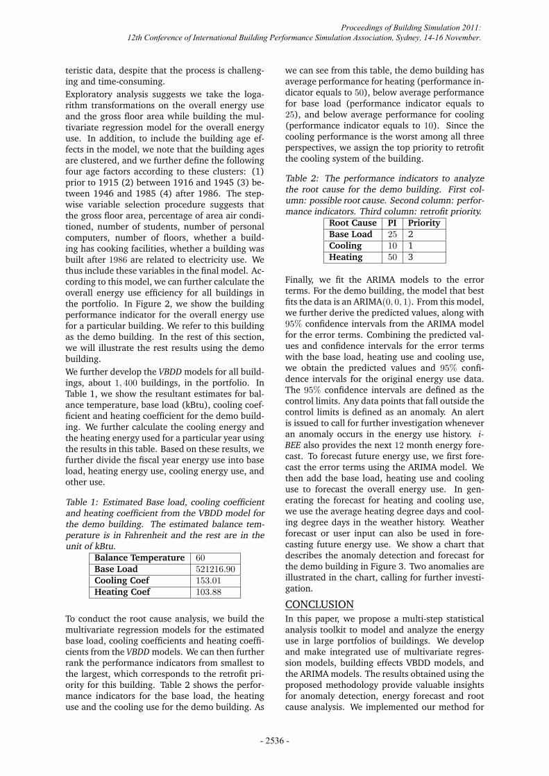
Finally, we fit the ARIMA models to the errorterms. For the demo building, the model that bestfits the data is an ARIMA(0, 0, 1). From this model,we further derive the predicted values, along with95% confidence intervals from the ARIMA modelfor the error terms. Combining the predicted val-ues and confidence intervals for the error termswith the base load, heating use and cooling use,we obtain the predicted values and 95% confi-dence intervals for the original energy use data.The 95% confidence intervals are defined as thecontrol limits. Any data points that fall outside thecontrol limits is defined as an anomaly. An alertis issued to call for further investigation wheneveran anomaly occurs in the energy use history. i-BEE also provides the next 12 month energy fore-cast. To forecast future energy use, we first fore-cast the error terms using the ARIMA model. Wethen add the base load, heating use and coolinguse to forecast the overall energy use. In gen-erating the forecast for heating and cooling use,we use the average heating degree days and cool-ing degree days in the weather history. Weatherforecast or user input can also be used in fore-casting future energy use. We show a chart thatdescribes the anomaly detection and forecast forthe demo building in Figure 3. Two anomalies areillustrated in the chart, calling for further investi-gation.

CONCLUSIONIn this paper, we propose a multi-step statisticalanalysis toolkit to model and analyze the energyuse in large portfolios of buildings. We developand make integrated use of multivariate regres-sion models, building effects VBDD models, andthe ARIMA models. The results obtained using theproposed methodology provide valuable insightsfor anomaly detection, energy forecast and rootcause analysis. We implemented our method for


- 2536 -




Outside Control Limits:

Anomaly Usage

Figure 3: Anomaly detection and energy forecastfor the demo building (x-axis: month, y-axis: siteenergy use in kBtu). Anomaly detection periodstarts from the beginning of the trajectory andends before the start of the green vertical bar.Forecast period begins after the green vertical bar.In the picture, the blue line represents the actualenergy use; dashed yellow lines represent the up-per control limit (UCL) and lower control limit(LCL); the red line represents the predicted val-ues for the energy use.

the NYC K-12 public school building portfolio anddemonstrated its usefulness. Finally, we remarkthat the methodology proposed in this paper doesnot reflect the uncertain user behaviors. To fur-ther investigate the impact of user behaviors, it isessential to study the building energy consump-tions with different user behaviors. “The NewYork City Public Schools Green Cup Challenge”(GreenCupChallenge), as one of such efforts, hastaken place between March 4th and April 1, 2011.The research contents presented in this paper areour initial efforts to develop a statistics basedtoolkit for analyzing energy consumption of build-ing portfolios. Another thread of research ac-tivities at IBM is to develop physics based mod-els using inverse modeling and parameter esti-mation techniques. Directly based on heat andmass transport phenomena, these models provideestimates for heat transfer parameters with realphysical meanings, such as the R-value for roof,R-value for wall, U-value for windows, and in-filtration coefficient. It would be of interest tocombine the strengths of statistical methods withphysics based models through integrated model-ing, where information produced from one typeof modeling is used for the other type of model-ing. We plan to pursue this direction in our futureresearch and development.

ACKNOWLEDGEMENTWe wish to thank our colleagues contributingto this project: Paul Nevill, Estepan Melikse-tian, Pawan Chowdhary, Lianjun An, Raya Horesh,

Chandra Reddy, Young Tae Chae of IBM Reseach;Janine Belfest of Optimal Green Operations.

REFERENCESBrockwell, P. J. and Davis, R. A. 2006. Time Series:

Theory and Methods. Springer, 2 edition.

DOE 2007. Buildings energy data book.

DOE 2008a. http://www.eia.doe.gov/oiaf/1605/ggrpt/carbon.html.

DOE 2008b. Assumptions to the annual energyoutlook.

DOE 2008c. Eia annual energy outlook.

EPA 2009. Energy star performance ratings: Tech-nical methodology. United States EnvironmentProtection Agency.

GreenCupChallenge. http://www.greencupchallenge.net/nyc/.

IBM 2011. City university of new york and ibmto reduce energy consumption in public schoolbuildings. http://www.ibm.com/press/us/en/pressrelease/34080.wss.

IPCC 2007. Ipcc fourth assessment re-port: Climate change 2007: Mitiga-tion of climate change. http://www.ipcc.ch/publications_and_data/publications_and_data_reports.htm#1.

Kissock, J. K., Haberl, J., and Claridge, D. E. 2003.Inverse modeling toolkit (1050rp): Numericalalgorithms. ASHRAE Transactions, 109:425–434.

PLANYC 2007. Planyc 2030: A greener, greaternew york. http://www.nyc.gov/html/planyc2030/html/home/home.shtml.

Schwarz, G. E. 1978. Estimating the dimension ofa model. Annals of Statistics, 6(2):461–464.

WBCDS 2009. Transforming the market: Energyefficiency in buildings.


- 2537 -

Documents

STATISTICAL MODELING FOR ANOMALY DETECTION, · PDF fileSTATISTICAL MODELING FOR ANOMALY DETECTION, FORECASTING AND ROOT CAUSE ANALYSIS OF ENERGY ... is the IBM Building Energy