Time step restrictions for Runge-Kutta

discontinuous Galerkin methods on triangular

grids

Ethan J. Kubatko a, Clint Dawson a, Joannes J. Westerink b

aInstitute for Computational Engineering and Sciences, The University of Texas

at Austin, Austin, TX 78712, United States

bDepartment of Civil Engineering and Geological Sciences, University of Notre

Dame, Notre Dame, IN 46556, United States

Abstract

We derive CFL conditions for the so-called Runge-Kutta Discontinuous Galerkin(RKDG) methods on triangular grids. Semidiscrete DG approximations using poly-nomials spaces of degree p = 0, 1, 2, and 3 are considered and discretized intime using a number of different strong-stability-preserving (SSP) Runge-Kuttatime discretization methods. Two structured triangular grid configurations are an-alyzed for wave propagation in different directions. Approximate relations betweenthe two-dimensional CFL conditions derived here and previously established one-dimensional conditions can be observed after defining an appropriate triangulargrid parameter h and a constant that is dependent on the polynomial degree p ofthe DG spatial approximation. Numerical results verify the CFL conditions thatare obtained, and “optimal”, in terms of computational efficiency, two-dimensionalRKDG methods of a given order are identified.

Key words:

discontinuous Galerkin, strong-stability-preserving, Runge-Kutta

1 Introduction

Runge-Kutta discontinuous Galerkin (RKDG) methods are a widely used ap-proach for the solution of time-dependent, hyperbolic and advection domi-nated advection-diffusion equations — see, for example, [1,2,5–9,14,19]. Themethods have been used to model a wide range of physical phenomena such asgas dynamics, electromagnetics, shallow water flow, and advection of contam-inants. Application of RKDG methods proceeds along the classical notions of

Preprint submitted to Elsevier Science 6 August 2008

the method of lines whereby the partial differential equation(s) (PDEs) arefirst discretized in space using a DG method, which produces a system ofordinary differential equations (ODEs), and then discretized in time using aspecial class of explicit RK time discretization methods. When using explicitmethods it is well known that the grid spacing and the time step ∆t that areemployed must satisfy a CFL condition in order to guarantee stability.

For RKDG methods using DG spatial discretizations of polynomials of degreep = k − 1 and a k stage RK method of order k (such a method is referred toas a k-th order RKDG method), Cockburn and Shu [9] give an approximateCFL condition of the form:

|c|∆t

∆x≤ 1

2p + 1(1)

where |c| is the wave speed associated with the given problem and ∆x is theuniform grid spacing. This condition is, in fact, exact for the cases p = 0 andp = 1 (the case p = 0 can be proven trivially and the case p = 1 was provenin [7]). Furthermore, for p ≥ 2, this estimate was observed to be less than 5%smaller than numerically-obtained estimates of the CFL condition [9].

Given the somewhat restrictive nature of (1), especially as p increases, thestability of RKDG methods using so-called strong-stability-preserving (SSP)RK methods where the number of stages s is greater than the order k ofthe method were examined in [15] with the goal of obtaining more efficientRKDG methods. Necessary time step restrictions for stability were derivedand “optimal” RKDG methods, in terms of computationally efficiency, wereidentified. For an RKDG method of a given order, the computational efficiencyis a function of both the CFL condition and the number of stages of the SSPRK method. In the majority of cases examined in [15], use of the s > kSSP RK methods was more efficient than the standard practice of using thes = k methods. This was due to gains in allowable time step size affordedby improved CFL conditions that were large enough to offset the additionalwork introduced by the increased number of stages. It was found that optimalRKDG methods were generally obtained by using one or two additional stagesthan theoretically required for a given order.

The work cited above has been for one-dimensional RKDG methods. In recentnumerical experiments, we have noted that simple two-dimensional analogsof these CFL conditions do not appear to be sufficient for stability in two-dimensions on structured triangular grids. Therefore, in this paper, we seek toextend the types of one-dimensional analyses performed in [7,9,15] to RKDGmethods in two-dimensions. Specifically, we derive necessary time step restric-tions, which also appear to be sufficient, for the stability of RKDG methods onstructured triangular grids applied to the constant coefficient, two-dimensional

2

transport equation with periodic boundary conditions. Two different struc-tured triangular grid patterns are examined on which we consider wave prop-agation in different directions. For these grids, the stability of RKDG meth-ods of order k = 1, 2, 3, and 4 are considered. In the case of the first-orderRKDG method, which is equivalent to a first-order finite volume method, CFLconditions are derived analytically by first constructing the semidiscrete DGequations over a repeating grid generation pattern, explicitly computing theeigenvalues of the resulting matrices, and then calculating the necessary re-strictions so that, when scaled by the time step ∆t, these eigenvalues lie withinthe stability region of a given RK method. For the first-order RKDG method,an exact relationship between the one- and two-dimensional CFL conditionsis found once an appropriate triangular grid spacing parameter h is defined.For the higher-order methods, we use a semi-analytical approach in which thediscrete equations are explicitly constructed as before but with the eigenval-ues of the resulting matrices being computed numerically and then checkedfor the stability condition at a discrete number of points. In the high-ordercases, approximate relationships between the one- and two-dimensional CFLconditions can be observed using the previously defined grid parameter h anda constant that is dependent on the polynomial degree p of the DG spatialdiscretization. The validity of these derived CFL conditions are demonstratedon numerical examples.

This paper is outlined as follows. First, in section 2, we give a brief overview ofthe DG spatial discretization of the linear, two-dimensional transport equationusing triangular elements, and we present the two structured, triangular gridpatterns that will be considered in our stability analysis. Next, in section 3, wereview some aspects of RK time stepping methods that are pertinent to ourobjective of deriving CFL conditions. We begin by presenting the general formof the RK methods that are used and the so-called SSP theorem in section3.1 — noting some important facts related to this theorem that are specificto the application of SSP RK methods to the semidiscrete DG equations.This is followed by a brief overview of the stability of RK methods in section3.2. We then derive CFL conditions for RKDG methods using polynomialsspaces of degree p = 0, 1, 2, and 3 and “matching order” SSP RK methods insection 4. Several different SSP RK methods are examined, ranging from twoto eight stages, and “optimal” two-dimensional RKDG methods, in terms ofcomputational efficiency, are identified for a given order. This is followed bya brief subsection in which approximate relationships between the one- andtwo-dimensional RKDG CFL conditions are established. Finally, in section 5,numerical results are presented that verify our stability analysis.

3

u−

h

u+

h

ne

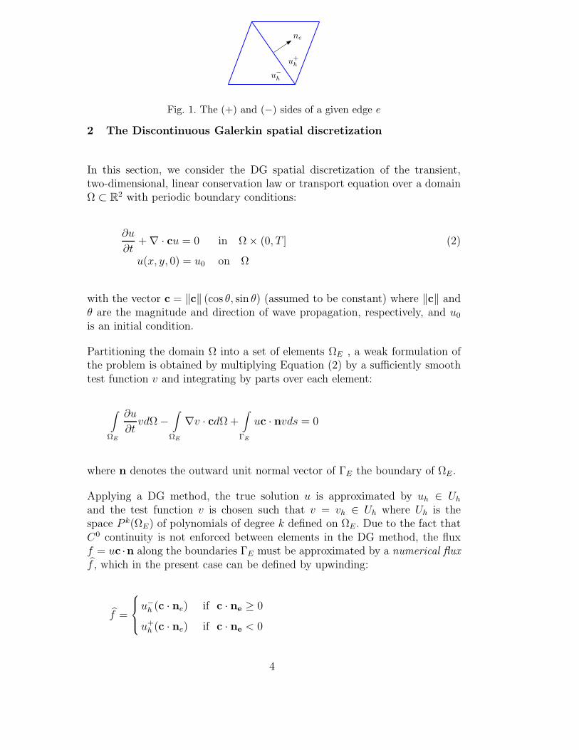
Fig. 1. The (+) and (−) sides of a given edge e

2 The Discontinuous Galerkin spatial discretization

In this section, we consider the DG spatial discretization of the transient,two-dimensional, linear conservation law or transport equation over a domainΩ ⊂ R2 with periodic boundary conditions:

∂u

∂t+ ∇ · cu = 0 in Ω × (0, T ] (2)

u(x, y, 0) = u0 on Ω

with the vector c = ‖c‖ (cos θ, sin θ) (assumed to be constant) where ‖c‖ andθ are the magnitude and direction of wave propagation, respectively, and u0

is an initial condition.

Partitioning the domain Ω into a set of elements ΩE , a weak formulation ofthe problem is obtained by multiplying Equation (2) by a sufficiently smoothtest function v and integrating by parts over each element:

∫

ΩE

∂u

∂tvdΩ −

∫

ΩE

∇v · cdΩ +∫

ΓE

uc · nvds = 0

where n denotes the outward unit normal vector of ΓE the boundary of ΩE .

Applying a DG method, the true solution u is approximated by uh ∈ Uh

and the test function v is chosen such that v = vh ∈ Uh where Uh is thespace P k(ΩE) of polynomials of degree k defined on ΩE . Due to the fact thatC0 continuity is not enforced between elements in the DG method, the fluxf = uc ·n along the boundaries ΓE must be approximated by a numerical fluxf , which in the present case can be defined by upwinding:

f =

u−h (c · ne) if c · ne ≥ 0

u+h (c · ne) if c · ne < 0

4

x

(x2, y2)

(x3, y3)

(x1, y1)

y

ζ2

ζ1

(−1,−1) (1,−1)

(−1, 1)

Fig. 2. Definition of the master element in the local (ζ1, ζ2) coordinate system.

where u−h and u+

h are the DG solution values computed on the (−) and (+)sides of the edge, respectively, as shown in Figure 1, which is dictated by theorientation of the outward unit normal ne of an edge e.

Thus, the discrete weak form of the problem takes the following form:

∫

ΩE

∂uh

∂tvhdΩ −

∫

ΩE

∇vh · cdΩ +∫

ΓE

f vhds = 0

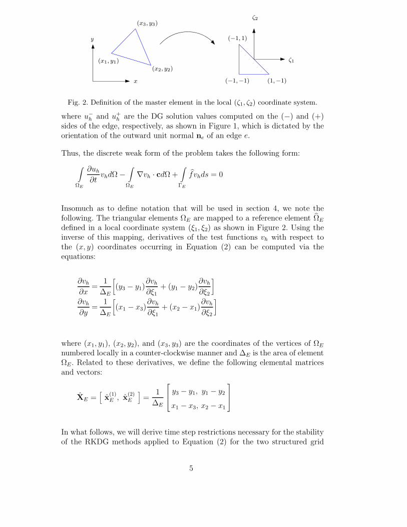
Insomuch as to define notation that will be used in section 4, we note thefollowing. The triangular elements ΩE are mapped to a reference element ΩE

defined in a local coordinate system (ξ1, ξ2) as shown in Figure 2. Using theinverse of this mapping, derivatives of the test functions vh with respect tothe (x, y) coordinates occurring in Equation (2) can be computed via theequations:

∂vh

∂x=

1

∆E

[(y3 − y1)

∂vh

∂ξ1+ (y1 − y2)

∂vh

∂ξ2

]

∂vh

∂y=

1

∆E

[(x1 − x3)

∂vh

∂ξ1

+ (x2 − x1)∂vh

∂ξ2

]

where (x1, y1), (x2, y2), and (x3, y3) are the coordinates of the vertices of ΩE

numbered locally in a counter-clockwise manner and ∆E is the area of elementΩE . Related to these derivatives, we define the following elemental matricesand vectors:

XE =[x

(1)E , x

(2)E

]=

1

∆E

y3 − y1, y1 − y2

x1 − x3, x2 − x1

In what follows, we will derive time step restrictions necessary for the stabilityof the RKDG methods applied to Equation (2) for the two structured grid

5

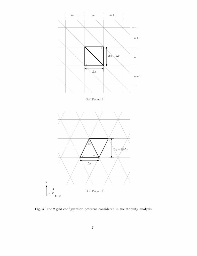
configurations shown in Figure 3, which can be thought of as being obtainedby simply repeating the grid generation patterns shown in bold in block m,n. Grid pattern I consists of right isosceles triangles obtained by bisecting asquare grid pattern to the left. Grid pattern II is made of equilateral triangles.Note also in Figure 3 that we define the direction of propagation θ with respectto the x-axis (counterclockwise positive).

3 Runge-Kutta methods

In this section, we review some aspects of RK methods that are pertinent tothe present analysis.

3.1 Strong-stability-preserving Runge-Kutta methods

Consider an explict s-stage RK method written in the so-called Shu-Osherrepresentation [20]:

u(0) = un

u(i) =i−1∑

l=0

αilu

(l) + ∆tβilF (u(l))

, i = 1, 2, . . . , s (3)

un+1 = u(s)

If, in addition to the constraints placed on αil and βil relating to order (see,for example, [3]) and consistency (

∑i−1l=0 αil = 1, i = 1, 2, . . . , s), the following

additional constraints are enforced:

(i) αil ≥ 0 and βil ≥ 0

(ii)αil = 0 only if βil = 0 (4)

then the RK method can be written as a convex combination of forward Eulersteps with time step sizes βil

αil∆t, i.e.:

u(0) = un

u(i) =i−1∑

l=0

αil

u(l) + ∆tβil

αilF (u(l))

, i = 1, 2, . . . , s

un+1 = u(s).

6

∆x

∆y = ∆x

θ

∆y =√

3

2∆x

Grid Pattern I

Grid Pattern II

60

m m + 1m − 1

n

n − 1

n + 1

∆x

60

60

x

y

Fig. 3. The 2 grid configuration patterns considered in the stability analysis

7

Such a RK method is referred to as a strong-stability-preserving (SSP) RKmethod, the name being based on the following theorem (see, for example,[13]):

Theorem 1 (The SSP Theorem) If the forward Euler method applied tothe spatial discretization F is (strongly) stable under the CFL condition ∆t ≤∆tFE then the Runge-Kutta method (3) with constraints (4) preserves thatstability under the CFL condition:

∆t ≤ κ∆tFE (5)

where κ ≡ mini,l

(αil

βil).

Much of the research in the area of SSP methods has focused on findingoptimal SSP RK methods — that is, the SSP RK method (5) for which κis a maximum under the given constraints placed on the αil and βil, see, forexample, [18].

It is interesting to note, however, that the SSP Theorem does not provide thecriteria for linear (L2) stability of the SSP RK methods applied to semidis-crete p = k − 1 DG approximations with k ≥ 2, due to the fact that forthese cases the forward Euler method applied to the semidiscrete equations isunconditionally-unstable for a fixed Courant number ν ≡ c∆t/∆x. This wasproven explicitly for the case k = 2 in [4], and the result carries over to allp = k − 1 DG spatial discretizations for k ≥ 2 [7]. Thus, in order to establishnecessary time step restrictions for the linear stability of the RKDG methodsthe complete RK method must be analyzed. This is discussed in more detailin the next subsection.

The condition given in Theorem 1 does, however, play a role in the establish-ing the time step criteria necessary for the TVD (or TVB) property of theRKDG method (and also the linear stability of the k = 1 RKDG case), sinceto establish the TVD (TVB) property of the RKDG methods a slope limiter isapplied that renders the forward Euler method TV-stable under an appropri-ate CFL condition (see, for example, [9]). In two-dimensions, where enforcingthe TVD property is incompatible with higher-order accuracy [11], a slopelimiter can be applied to enforce a maximum principle when using the for-ward Euler method. The timestep restriction for TV-stability or enforcementof a maximum principle for a given SSP RK method is then provided by con-dition (5). However, in general, these conditions are much weaker than thoserequired for linear stability, and, as pointed out in [9] and as demonstratednumerically in [15], it is the linear stability condition that must be respected orthe high-order accuracy of the methods will degenerate to first-order. This factprompted the investigation of the class of stage-exceeding-order (i.e. s > k)SSP RK methods applied to the semidiscrete DG equations presented in [15]

8

in order to determine one-dimensional RKDG methods that are optimal interms of computational efficiency, which is function of both the CFL condi-tions for linear stability and the number of stages of a given RK method. Inall the cases examined in that work, optimal RKDG methods were obtainedusing RK methods with one or more additional stages than the order of themethod. For this reason, the s > k RK methods are also examined here in thetwo-dimensional setting.

3.2 The stability of Runge-Kutta methods

Associated with each s-stage, k-th order RK method is a so-called charac-teristic polynomial Ps,k obtained by applying the given RK method to theprototypical, scalar equation u = λu where λ ∈ C, which can be written inthe form un+1 = Ps,k(z = ∆tλ)un. For example, the classic 2-stage, 2nd-orderRK method (or modified Euler method) written in the Shu-Osher representa-tion applied to this equation gives:

u(1) = un + zun

un+1 =1

2un +

1

2u(1) +

1

2z2u(1).

Substituting u(1) into the equation for u(n+1) and simplifying gives:

un+1 =(1 + z +

1

2z2

)

︸ ︷︷ ︸P2,2(z)

un.

Thus, stability of the RK method is guaranteed provided:

|Ps,k(z)| ≤ 1 (6)

where | · | is the complex modulus |x + iy| =√

x2 + y2 (x and y are realnumbers and i =

√−1). The set in the complex plane for which condition (6)

is satisfied is the so-called region of absolute stability S of the given Runge-Kutta method, that is:

S = z : |Ps,k(z)| ≤ 1| .

In terms of S then, condition (6) can be written as:

∆tλ ⊆ S. (7)

9

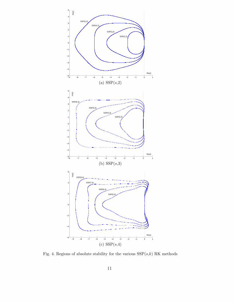
In Figure 4, we plot the regions of absolute stability for several of the SSP RKmethods considered here where we have used the notation SSP(s,k) to denotean s stage, k-th order SSP RK method.

In the case of applying an RK method to a system of equations, i.e. when thescalar λ in the equation considered above is replaced by a matrix Lh, the issueof stability is a more delicate issue. If the matrix Lh is normal (see, for example,[22]) then stability is guaranteed if condition (7) holds for each eigenvalue λof Lh. In the general case, however, condition (7) is only a necessary, and nota sufficient, condition for stability. Necessary and sufficient conditions in thegeneral (non-normal) case can be expressed in terms of the pseudospectra ofLh, see, for example, [16]. Here, with the exception of the k = 1 RKDG case,we will content ourselves with finding necessary conditions according to (7).These conditions also appear to be sufficient as will be demonstrated in thenumerical results section.

4 Stability Analysis

The discrete equations for the grid generation patterns shown in Figure 3 canbe written in the following compact form:

Md

dtUm,n = AUm,n − B±Um±1,n − C±Um,n±1 (8)

where Um,n is a vector containing the degrees of freedom for both of theelements in the grid block m, n (refer to Figure 3), i.e.:

Um,n =

u1

u2

.

Here u1 and u2 are vectors of length Nd containing the degrees of freedomof elements 1 and 2, respectively, of the given grid configuration (Nd = (p +1)(p + 2)/2 for a degree p triangular element). The mass matrix M is blockdiagonal:

M =

m1 0

0 m2

10

−9 −8 −7 −6 −5 −4 −3 −2 −1 0 1−5

−4

−3

−2

−1

0

1

2

3

4

5

SSP(2,2)

SSP(3,2)

SSP(4,2)

SSP(5,2)

Im(z

)Re(z)

(a) SSP(s,2)

−8 −7 −6 −5 −4 −3 −2 −1 0 1−5

−4

−3

−2

−1

0

1

2

3

4

5

Im(z

)

Re(z)

SSP(6,3)

SSP(5,3)

SSP(4,3)

SSP(3,3)

(b) SSP(s,3)

−9 −8 −7 −6 −5 −4 −3 −2 −1 0 1−6

−4

−2

0

2

4

6

Re(z)

Im(z

)

SSP(5,4)

SSP(6,4)

SSP(7,4)

SSP(8,4)

(c) SSP(s,4)

Fig. 4. Regions of absolute stability for the various SSP(s,k) RK methods

11

with blocks mE , the elemental mass matrices, given by:

mE =∆E

2m, mij =

∫

ΩE

φiφjdΩE .

where mij is the ij-th entry of the matrix m.

The matrix A is made up of both elemental and edge contributions:

A = AE + Ae

The matrix AE, like the mass matrx, is block diagonal with the blocks givenby:

aE =2∑

k=1

(c · x(k)E )a(k), a

(k)ij =

∫

Ωe

∂φi

∂ξkφjdΩE

The matrix Ae corresponds to contributions from the edge integrals that areinterior to the grid generation pattern and the outflow edges on the boundaryof the grid generation pattern. It is made up of blocks ae:

ae =l

2(c · n)a, aij =

∫

e

φiφjds

The matrices B and C are made up of the same blocks ae, but corresponding toedges that are inflow edges on the boundary of the grid generation pattern. Thestructure of these matrices changes based on the wave propagation direction θ,which dictates the upwind direction. For example, the matrices of grid patternI for 0 ≤ θ ≤ π/2 and grid pattern II for 0 ≤ θ ≤ π/3 will have the followingstructures:

Ae =

X, 0

X, X + X

, B− =

0, X

0, 0

, C− =

0, X

0, 0

where the X’s correspond to the matrices ae of a particular edge.

Following the ideas of classic Von Neumann stability analysis (see, for example,[17]), we seek a solution in the following form:

Um,n = Um,nei(kxm∆x+kyn∆y)

12

where kx and ky are wave numbers associated with the x and y directions,respectively. Substituting this into Equation (8) and inverting the mass matrix,the following equation is obtained:

d

dtUm,n = LhUm,n

where the matrix Lh, the DG spatial operator, is defined as:

Lh ≡ M−1(A −B±e±ikxm∆x − C±e±ikyn∆y

).

4.1 First-order RKDG method (k = 1)

The first-order RKDG method, which uses piecewise constants for the DGspatial discretization and the first-order forward Euler method in time, can beexamined analytically. As an example, we consider the problem of propagationin the range 0 ≤ θ ≤ π/2 on the first grid pattern. For this case, the matrixLh is given by:

Lh = 2 ‖c‖ 1

∆x

cos θ

−1 e−iα

1 −1

+ sin θ

−1 e−iβ

1 −1

where α ≡ kxm∆x, β ≡ kyn∆y ∈ [0, 2π] (note ∆x = ∆y for grid pattern I).It is a simple matter to verify that this is a normal matrix so condition (7) isnecessary and sufficient for stability. We explicitly compute the eigenvalues ofLh:

λ± = −2 ‖c‖ 1

∆x

[Θ ±

√Θ(Θc − iΘs)

]

where:

Θ ≡ cos θ + sin θ

Θc ≡ cos θ cos α + sin θ cos β

Θs ≡ cos θ sin α + sin θ sin β

The stability condition (6) must be satisifed for z = ∆tλ±. The characteristicpolynomial of the forward Euler method is simply P1,1 = 1 + z and so, in this

13

case, assuming the separation of λ± into real Re and imaginary Im parts,condition (6) reads:

|P1,1(z)|2 = 1 + ν[

2Re(Λ±) + ν(Re(Λ±)2 + Im(Λ±)2

) ]≤ 1, (9)

where Λ± ≡ λ±∆x/‖c‖ and ν is the Courant number (in two-dimensions weare initially defining this as ν = c∆t/∆x). Assuming that both Re(Λ±) 6= 0and Im(Λ±) 6= 0, inequality (9) can only be satisfied for ν > 0 provided:

ν ≤ ν ≡ −2Re(Λ±)

Re(Λ±)2 + Im(Λ±)2. (10)

With the help of the following identity for the square root of a complex number(see, for example, [21]):

√x + iy =

√2

2

√√x2 + y2 + x + i sgn(y)

√2

2

√√x2 + y2 − x,

the left side of (10) can be written in the form:

ν =1

2Θ

Re(Λ±)

Re(Λ±) + (Θ −√

Θ2c + Θ2

s)

.

where:

Re(Λ±) = −[2Θ ±

√2Θ(

√Θ2

c + Θ2s + Θc)

].

It can be shown that Re(Λ±) ≤ 0 and that 0 ≤ Θ −√

Θ2c + Θ2

s ≤ −Re(Λ±).

Thus, ν has a minimum value of 1/2Θ over the range of all α and β, and thecondition for stability is simply:

ν ≤ ν =1

2Θ.

Recall that this expression is valid for directions of propagation 0 ≤ θ ≤ π/2on grid pattern I, which corresponds to 1 ≤ Θ ≤

√2. In this range, the

stability condition is most restrictive at θ = π/4, in which case ν ≤√

2/4,and least restrictive at θ = 0 and π/2 when the direction of propagation isalong the shorter element edges, in which case ν ≤ 1/2.

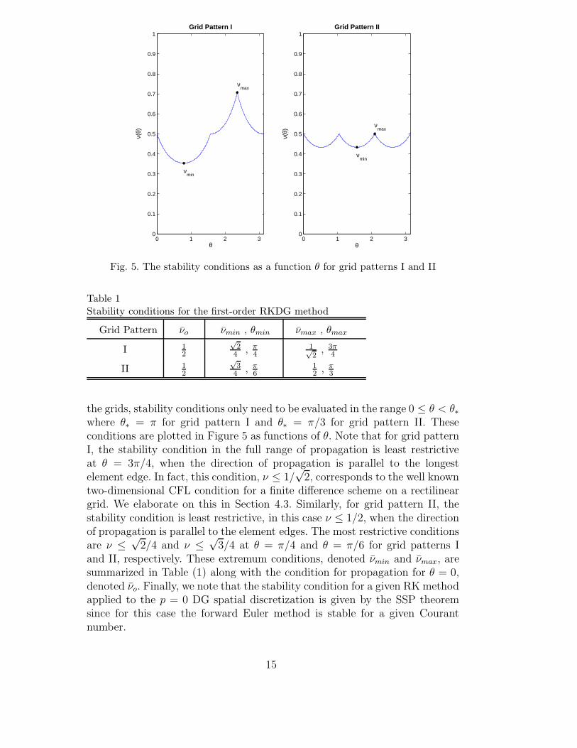
Stability conditions for the full spectrum of propagation directions for gridpatterns I and II can be derived in an analogous manner. Due to symmetry of

14

0 1 2 30

0.1

0.2

0.3

0.4

0.5

0.6

0.7

0.8

0.9

1

θ

ν(θ)

Grid Pattern I

0 1 2 30

0.1

0.2

0.3

0.4

0.5

0.6

0.7

0.8

0.9

1

θ

ν(θ)

Grid Pattern II

νmin

νmax

νmin

νmax

Fig. 5. The stability conditions as a function θ for grid patterns I and II

Table 1Stability conditions for the first-order RKDG method

Grid Pattern νo νmin , θmin νmax , θmax

I 12

√2

4 , π4

1√2

, 3π4

II 12

√3

4 , π6

12 , π

3

the grids, stability conditions only need to be evaluated in the range 0 ≤ θ < θ∗where θ∗ = π for grid pattern I and θ∗ = π/3 for grid pattern II. Theseconditions are plotted in Figure 5 as functions of θ. Note that for grid patternI, the stability condition in the full range of propagation is least restrictiveat θ = 3π/4, when the direction of propagation is parallel to the longestelement edge. In fact, this condition, ν ≤ 1/

√2, corresponds to the well known

two-dimensional CFL condition for a finite difference scheme on a rectilineargrid. We elaborate on this in Section 4.3. Similarly, for grid pattern II, thestability condition is least restrictive, in this case ν ≤ 1/2, when the directionof propagation is parallel to the element edges. The most restrictive conditionsare ν ≤

√2/4 and ν ≤

√3/4 at θ = π/4 and θ = π/6 for grid patterns I

and II, respectively. These extremum conditions, denoted νmin and νmax, aresummarized in Table (1) along with the condition for propagation for θ = 0,denoted νo. Finally, we note that the stability condition for a given RK methodapplied to the p = 0 DG spatial discretization is given by the SSP theoremsince for this case the forward Euler method is stable for a given Courantnumber.

15

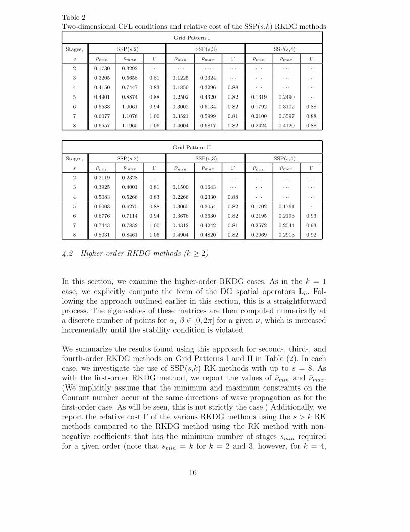
Table 2Two-dimensional CFL conditions and relative cost of the SSP(s,k) RKDG methods

Grid Pattern I

Stages, SSP(s,2) SSP(s,3) SSP(s,4)

s νmin νmax Γ νmin νmax Γ νmin νmax Γ

2 0.1730 0.3292 · · · · · · · · · · · · · · · · · · · · ·3 0.3205 0.5658 0.81 0.1225 0.2324 · · · · · · · · · · · ·4 0.4150 0.7447 0.83 0.1850 0.3296 0.88 · · · · · · · · ·5 0.4901 0.8874 0.88 0.2502 0.4320 0.82 0.1319 0.2490 · · ·6 0.5533 1.0061 0.94 0.3002 0.5134 0.82 0.1792 0.3102 0.88

7 0.6077 1.1076 1.00 0.3521 0.5999 0.81 0.2100 0.3597 0.88

8 0.6557 1.1965 1.06 0.4004 0.6817 0.82 0.2424 0.4120 0.88

Grid Pattern II

Stages, SSP(s,2) SSP(s,3) SSP(s,4)

s νmin νmax Γ νmin νmax Γ νmin νmax Γ

2 0.2119 0.2328 · · · · · · · · · · · · · · · · · · · · ·3 0.3925 0.4001 0.81 0.1500 0.1643 · · · · · · · · · · · ·4 0.5083 0.5266 0.83 0.2266 0.2330 0.88 · · · · · · · · ·5 0.6003 0.6275 0.88 0.3065 0.3054 0.82 0.1702 0.1761 · · ·6 0.6776 0.7114 0.94 0.3676 0.3630 0.82 0.2195 0.2193 0.93

7 0.7443 0.7832 1.00 0.4312 0.4242 0.81 0.2572 0.2544 0.93

8 0.8031 0.8461 1.06 0.4904 0.4820 0.82 0.2969 0.2913 0.92

4.2 Higher-order RKDG methods (k ≥ 2)

In this section, we examine the higher-order RKDG cases. As in the k = 1case, we explicitly compute the form of the DG spatial operators Lh. Fol-lowing the approach outlined earlier in this section, this is a straightforwardprocess. The eigenvalues of these matrices are then computed numerically ata discrete number of points for α, β ∈ [0, 2π] for a given ν, which is increasedincrementally until the stability condition is violated.

We summarize the results found using this approach for second-, third-, andfourth-order RKDG methods on Grid Patterns I and II in Table (2). In eachcase, we investigate the use of SSP(s,k) RK methods with up to s = 8. Aswith the first-order RKDG method, we report the values of νmin and νmax.(We implicitly assume that the minimum and maximum constraints on theCourant number occur at the same directions of wave propagation as for thefirst-order case. As will be seen, this is not strictly the case.) Additionally, wereport the relative cost Γ of the various RKDG methods using the s > k RKmethods compared to the RKDG method using the RK method with non-negative coefficients that has the minimum number of stages smin requiredfor a given order (note that smin = k for k = 2 and 3, however, for k = 4,

16

smin = 5; see [12]). These values are computed based on the values of νmin.For example, while the SSP(3,2) RKDG method, which is found to be theoptimal second-order RKDG method, allows a time step roughly 1.85 timeslarger than the SSP(2,2) RKDG method it requires one additional evaluationof F . Thus, a given time T can be reached (assuming the maximum allowabletime step is used) at approximately 80% of the computational cost of theSSP(2,2) RKDG method. The optimal third-order method is achieved usingthe SSP(7,3) RK method although its efficiency is only marginally better thanthat of the SSP(5,3) method and requires more storage. Thus, in practice,the SSP(5,3) would most likely be more efficient. For the fourth-order RKDGmethods, all of the s > 5 RK methods offer roughly the same moderate savingsover the SSP(5,4) RK method.

From these results, it can also be observed that the differences between νmin

and νmax generally become less significant as both p and s are increased.For example, the ratio of νmin to νmax for the first-order RKDG method ongrid patterns I and II are 0.5 and 0.866 (≈

√3/2), respectively, while for the

higher-order methods, these ratios are 0.525 and 0.910, 0.527 and 0.913, and0.558 and 0.967 for the SSP(2,2), SSP(3,3), and SSP(5,4) RKDG methods,respectively. As an example of this trend with respect to the number of stagesfor a fixed value of p, it can be noted that for grid pattern II the ratio of νmin

to νmax is 0.910 for the SSP(2,2) RKDG method and 0.949 for the SSP(8,2)method. In fact, on grid pattern II it can be noted that for the third-orderRKDG methods with s > 5 and the fourth-order methods with s > 6 the νmin

are actually found to be slightly greater (though by < 2%) than the νmax.

4.3 Relation to one-dimension CFL conditions

It is interesting to attempt to relate these two-dimensional CFL conditions tothe one-dimensional conditions derived in [7] and [15] by defining a Courantnumber in terms of an appropriately defined grid parameter or “element di-ameter” h. Here, we have initially taken h to be the shortest element edge,i.e. h ≡ ∆x. Indeed, such an approach is often used in practice to select anappropriate time step (see, for example, [1,8,19]), i.e.

∆t ≤ h

‖c‖ ν1D (11)

where ν1D is the maximum Courant number that can be used in one-dimension.

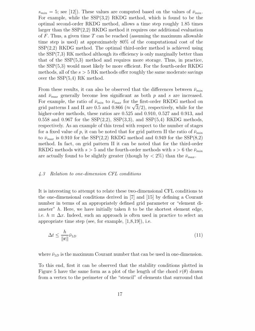
To this end, first it can be observed that the stability conditions plotted inFigure 5 have the same form as a plot of the length of the chord r(θ) drawnfrom a vertex to the perimeter of the “stencil” of elements that surround that

17

r(θ)

hmin =√

2

2∆x

θ

hmin =√

3

2∆x

Fig. 6. The distance r(θ) used to define an appropriate mesh spacing parameter h

for triangular grids

vertex; see Figure 6. Thus, if one defines a direction-dependent grid parameterhθ = r(θ) then for a given direction of wave propagation θ the two-dimensionalCFL conditions for the first-order RKDG method can be expressed in termsof hθ and the one-dimensional CFL condition simply as:

p = 0 : ‖c‖ ∆t

hθ≤ 1

2ν1D. (12)

Obviously, if a time step is to be selected that will be stable for wave propa-gation in an arbitrary direction then one must take:

p = 0 : ∆t ≤ 1

2

hmin

‖c‖ (13)

where hmin is the radius of the largest circle that is entirely contained withinthe stencil of elements surrounding a vertex (see Figure 6) and where we haveused the fact that ν1D = 1 for the first-order RKDG method. We remark thatthis definition of hmin has an obvious relation to the two-dimensional CFLcondition for a finite difference method on a rectilinear grid — namely, thatthe domain of dependence of a finite difference grid point, which is a sphericalcone in two dimensions, must be contained within the finite difference stencil;see [10]. Note that condition (13), which is necessary and sufficient for stability,is stricter than using condition (11) with h defined as the shortest element edgeor the diameter of the inscribed circle of the element — two approaches thatare commonly used in practice.

This simple result, however, does not hold for the higher-order RKDG meth-ods. However, for the second-order RKDG methods, it can be observed thatif the factor of 1/2 of condition (12) is replaced by 1/

√2 then one obtains a

good approximation of the two-dimensional CFL conditions reported in Table(2) in terms of their one-dimensional counterparts. This leads us to consider

18

Fig. 7. The initial condition used for the numerical test

the general condition:

‖c‖ ∆t

hθ≤ 1

21/(p+1)ν1D. (14)

Of course, for p = 0 we recover condition (11), which is an exact relation forthe two-dimensional CFL conditions expressed in terms of the one-dimensionalresults. For p = 1, the estimates provided by (14) for νmax are generally within2% of those reported in Table (2) for both grid patterns I and II (the onlyexception being the SSP(3,2) method, which is within 4%). For p = 2 andp = 3, these estimates are within 7% for grid pattern I and 5% for grid patternII. The estimates for νmin provided by (14) are less accurate — though theyare still within 10% of the computed values, with the errors increasing withthe number of stages.

5 Numerical results

In this section, we verify the various stability conditions obtained in the pre-vious section. We consider an initial condition given by a two-dimensionalGaussian function of the form:

u0(x, y) =A

2πσe−(x2+y2)/2σ2

. (15)

19

(a) Grid Pattern I

(b) Grid Pattern II

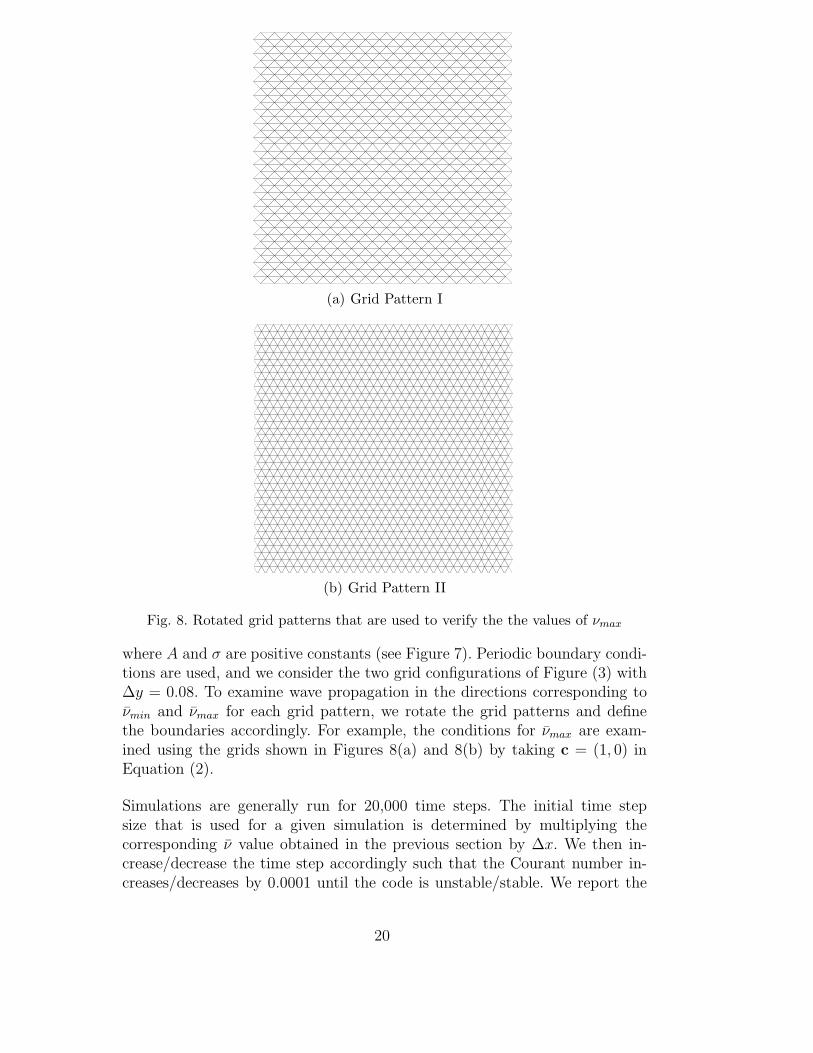
Fig. 8. Rotated grid patterns that are used to verify the the values of νmax

where A and σ are positive constants (see Figure 7). Periodic boundary condi-tions are used, and we consider the two grid configurations of Figure (3) with∆y = 0.08. To examine wave propagation in the directions corresponding toνmin and νmax for each grid pattern, we rotate the grid patterns and definethe boundaries accordingly. For example, the conditions for νmax are exam-ined using the grids shown in Figures 8(a) and 8(b) by taking c = (1, 0) inEquation (2).

Simulations are generally run for 20,000 time steps. The initial time stepsize that is used for a given simulation is determined by multiplying thecorresponding ν value obtained in the previous section by ∆x. We then in-crease/decrease the time step accordingly such that the Courant number in-creases/decreases by 0.0001 until the code is unstable/stable. We report the

20

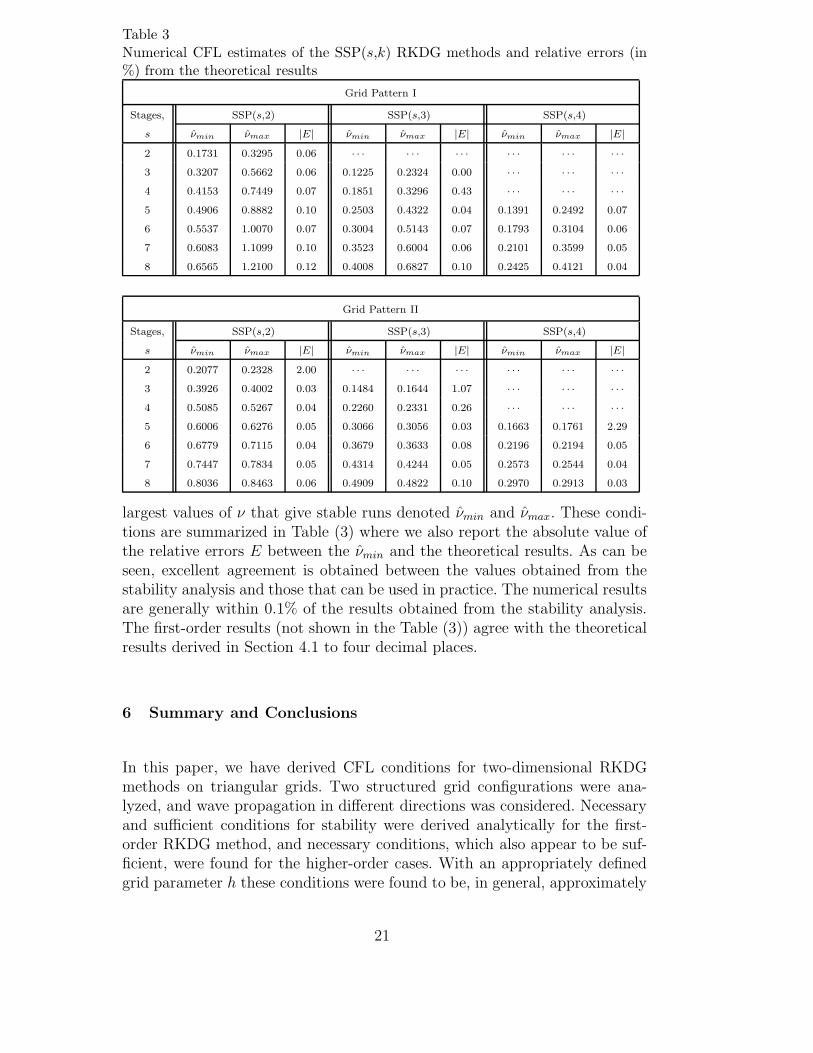
Table 3Numerical CFL estimates of the SSP(s,k) RKDG methods and relative errors (in%) from the theoretical results

Grid Pattern I

Stages, SSP(s,2) SSP(s,3) SSP(s,4)

s νmin νmax |E| νmin νmax |E| νmin νmax |E|2 0.1731 0.3295 0.06 · · · · · · · · · · · · · · · · · ·3 0.3207 0.5662 0.06 0.1225 0.2324 0.00 · · · · · · · · ·4 0.4153 0.7449 0.07 0.1851 0.3296 0.43 · · · · · · · · ·5 0.4906 0.8882 0.10 0.2503 0.4322 0.04 0.1391 0.2492 0.07

6 0.5537 1.0070 0.07 0.3004 0.5143 0.07 0.1793 0.3104 0.06

7 0.6083 1.1099 0.10 0.3523 0.6004 0.06 0.2101 0.3599 0.05

8 0.6565 1.2100 0.12 0.4008 0.6827 0.10 0.2425 0.4121 0.04

Grid Pattern II

Stages, SSP(s,2) SSP(s,3) SSP(s,4)

s νmin νmax |E| νmin νmax |E| νmin νmax |E|2 0.2077 0.2328 2.00 · · · · · · · · · · · · · · · · · ·3 0.3926 0.4002 0.03 0.1484 0.1644 1.07 · · · · · · · · ·4 0.5085 0.5267 0.04 0.2260 0.2331 0.26 · · · · · · · · ·5 0.6006 0.6276 0.05 0.3066 0.3056 0.03 0.1663 0.1761 2.29

6 0.6779 0.7115 0.04 0.3679 0.3633 0.08 0.2196 0.2194 0.05

7 0.7447 0.7834 0.05 0.4314 0.4244 0.05 0.2573 0.2544 0.04

8 0.8036 0.8463 0.06 0.4909 0.4822 0.10 0.2970 0.2913 0.03

largest values of ν that give stable runs denoted νmin and νmax. These condi-tions are summarized in Table (3) where we also report the absolute value ofthe relative errors E between the νmin and the theoretical results. As can beseen, excellent agreement is obtained between the values obtained from thestability analysis and those that can be used in practice. The numerical resultsare generally within 0.1% of the results obtained from the stability analysis.The first-order results (not shown in the Table (3)) agree with the theoreticalresults derived in Section 4.1 to four decimal places.

6 Summary and Conclusions

In this paper, we have derived CFL conditions for two-dimensional RKDGmethods on triangular grids. Two structured grid configurations were ana-lyzed, and wave propagation in different directions was considered. Necessaryand sufficient conditions for stability were derived analytically for the first-order RKDG method, and necessary conditions, which also appear to be suf-ficient, were found for the higher-order cases. With an appropriately definedgrid parameter h these conditions were found to be, in general, approximately

21

equal to the one-dimensional CFL conditions found in [6] and [15] times afactor that is a function of the degree of the DG spatial approximation p. Theobserved relationship between the one- and two-dimensional CFL conditionsis exact for the first-order case and provides a good approximation of the con-ditions for higher-order RKDG methods. As was found to be in the case inone-dimension, optimal, in terms of computational efficiency, two-dimensionalRKDG methods are obtained by using one or two additional stages than the-oretically required for a given order. The computational savings achieved byusing the s > k RK methods in two-dimensions are moderately better thanthose observed in the one-dimensional case. The derived CFL conditions wereverified on numerical examples.

Finally, although the CFL conditions were derived on structured grids, theycould also serve as reasonable estimates for unstructured grids with h beingdefined analogously to what is depicted in Figure (6). Additionally, based onthe results found here, one can conjecture that the CFL conditions for RKDGmethods on n-dimensional simplexes are given by a relation of the form:

‖c‖ ∆t

h≤ 1

nf(p)ν1D (16)

where h is a grid parameter defined analogously to the two-dimensional caseconsidered here. This will be investigated in future work.

Acknowledgements

This work was supported by National Science Foundation grants DMS 0620697and 0620696 and by the Office of Naval Research, Award Number: N00014-06-1-0285.

References

[1] V. Aizinger, C. Dawson, A discontinuous Galerkin method for two-dimensionalflow and transport in shallow water, Advances in Water Resources 25 (2002)67–84.

[2] V. Aizinger, C. Dawson, B. Cockburn, P. Castillo, The local discontinuousGalerkin method for contaminant transport, Advances in Water Resources 24(2001) 73–87.

[3] J.C. Butcher, The Numerical Analysis of Ordinary Differential Equations:Runge-Kutta and General Linear Methods, John Wiley, Chichester, 1987.

22

[4] G. Chavent, B. Cockburn, The local projection P 0 − P 1-discontinuous-Galerkinfinite element method for scalar conservation laws, Mathematical Modelling andNumerical Analysis 23 (1989) 565–592.

[5] M.H. Chen, B. Cockburn, F. Reitich, High-order RKDG methods forcomputational electromagnetics, Journal of Scientific Computing 22 and 23(2005) 205–226.

[6] B. Cockburn, C.W. Shu, TVB Runge-Kutta local projection discontinuousGalerkin finite element method for scalar conservation laws II: Generalframework, Mathematics of Computation 52 (1989) 411–435.

[7] B. Cockburn, C.W. Shu, The Runge-Kutta local projection P 1-discontinuous-Galerkin finite element method for scalar conservation laws, MathematicalModelling and Numerical Analysis 25 (1991) 337–361.

[8] B. Cockburn, S. Hou, C.W. Shu, The RungeKutta discontinuous Galerkinmethod for conservation laws V: Multidimensional systems. Journal ofComputational Physics 141 (1998) 199-224.

[9] B. Cockburn, C.W. Shu, Runge-Kutta discontinuous Galerkin methods forconvection dominated problems, Journal of Scientific Computing 16 (2001) 173–261.

[10] R. Courant, K. Friedrichs, H. Lewy, On the partial difference equations ofmathematical physics, Mathematische Annalen 100 (1928) 32–74.

[11] J. Goodman, R. LeVeque, On the accuracy of stable schemes for 2D scalarconservation laws, Mathematics of Computation 45 (1985) 15–21.

[12] S. Gottlieb, C.W. Shu, Total variation diminishing RungeKutta schemes,Mathematics of Computation 67 (1998) 73–85.

[13] S. Gottlieb, C.W. Shu, E. Tadmor, Strong stability-preserving high-order timediscretization methods, SIAM Review 43 (2001) 89–112.

[14] E.J. Kubatko, J.J. Westerink, C. Dawson, hp discontinuous Galerkin methodsfor advection dominated problems in shallow water flow, Computer Methods inApplied Mechanics and Engineering, Computer Methods in Applied Mechanicsand Engineering 196 (2006) 437-451.

[15] E.J. Kubatko, J.J. Westerink, C. Dawson, Semidiscrete discontinous Galerkinmethods and stage-exceeding-order, strong-stability-preserving Runge-Kuttatime discretizations, Journal of Computational Physics 222 (2007) 832–848.

[16] S.C. Reddy, L.N. Trefethen, Stability of the method of lines, NumerischeMathematik 62 (1992) 235–267.

[17] R.D. Richtmyer, K.W. Morton, Difference Methods for Initial-Value Problems,2nd ed., John Wiley, New York, 1967.

[18] S.J. Ruuth, Global optimization of explicit strong-stability-preserving Runge-Kutta methods, Mathematics of Computation 75 (2006) 183–207.

23

[19] D. Srmny, M.A. Botchev, J.J.W. van der Vegt, Dispersion and dissipation errorin high-order Runge-Kutta discontinuous Galerkin discretisations of the MaxwellEquations, J Sci Computing 33 (2007) 47-74.

[20] C.W. Shu, S. Osher, Efficient implementation of essentially non-oscillatoryshock-capturing schemes, Journal of Computational Physics 77 (1988) 439–471.

[21] J. Spanier, K.B. Oldham, An Atlas of Functions, Washington, DC: Hemisphere,1987.

[22] G. Strang, Linear algebra and its applications, Academic Press, New York, 1970.

24