Time Symmetry of Project Scheduling with Time Windows …mistaconference.org/2009/papers/239-253-101-P.pdf · Time Symmetry of Project Scheduling with Time Windows and Take ... An

MISTA 2009

Time Symmetry of Project Scheduling with Time

Windows and Take-give Resources

Zdenek Hanzalek · Premysl Sucha

Abstract The paper studies a real production scheduling problem with special re-

sources called take-give resources. Such resources are needed from the beginning of an

activity to the completion of another activity of the production process. The difference

to other works is that we consider sequence dependent changeover time on take-give

resources. We formulate this problem by integer linear programming and we suggest a

heuristic problem solution. In the second part of the paper we discuss how to construct

a schedule in backward time orientation and we formulate a time symmetry mapping.

Consequently it is shown that the mapping is bijective and involutive. Finally, perfor-

mance of the heuristic algorithm with the time symmetry mapping is evaluated on a

set of lacquer production benchmarks.

1 Introduction

The problem that we address in this paper is motivated by a real production scheduling

specifically by a lacquer production [1] which is seen as the project scheduling prob-

lem with general temporal and resource constraints. Temporal constraints between

activities of a project define minimal and maximal distance between activities, e.g.

a laboratory checking must be performed within a prescribed interval related to the

beginning of an activity of the lacquer production procedure. The resource constraints

express limits of renewable resources such as machines (e.g. lacquer mixers) or man-

power (e.g. laboratory technicians). In addition, there are special resources (mixing

vessels) that are needed from the beginning of an activity to the completion of another

activity. This is why we extend the classical resource constrained project scheduling

problem by so called take-give resources. Moreover we observe that each instance of

the problem can be transformed to another instance of the problem which is executed

Zdenek HanzalekDepartment of Control Engineering, Faculty of Electrical Engineering, Czech Technical Uni-versity in PragueE-mail: [email protected]

Premysl SuchaDepartment of Control Engineering, Faculty of Electrical Engineering, Czech Technical Uni-versity in PragueE-mail: [email protected]

Multidisciplinary International Conference on Scheduling : Theory and Applications (MISTA 2009) 10-12 August 2009, Dublin, Ireland

239

in inverse time. Based on this observation we define a time symmetry mapping and we

show that the mapping is bijective and involutive.

Various types of solutions of resource constrained project scheduling problems with

positive and negative time-lags have been proposed in literature. Most of exact algo-

rithms are based on branch and bound technique [3] but this approach is suitable for

problems with less than 100 activities [6]. A heuristic algorithm by Cesta et al [5] is

based on constraint satisfaction problem solving. The algorithm is based on the intu-

ition that the most critical conflicts to be resolved first are those involving activities

with large resource capacity requirements. Another heuristic algorithm proposed in [14]

combines the benefits of the “squeaky wheel” optimization with an effective conflict

resolution mechanism, called “bulldozing”. The possibility of improving on the squeaky

wheel optimization by incorporating aspects of genetic algorithms is suggested in [15].

An overview of heuristic approaches is shown in [6] where the authors compare trun-

cated branch and bound techniques, priority rule methods and schedule improvement

procedures. A beam search heuristic is applied in [6] to scheduling of rolling ingots

production. This problem cover renewable resources, changeover time and batching

machines.

Up to our knowledge, there is no work dealing with take-give resources in project

scheduling. Scheduling with blocking operations [11,4] can be seen as a subproblem of

scheduling with take-give resources. Operations are blocking if they must stay on a

machine after finishing when the next machine is occupied by another job. During this

stay the machine is blocked for other jobs, i.e. blocking operations models the absence

of storage capacity between machines. On the other hand, there is a more general

framework called reservoirs or storage resources [10] usually used to model limited

storage capacity or inventory limits. In this framework each activity can replenish or

deplete certain amount of a resource but the resource assignment is not considered.

Therefore this framework can not deal for example with changeover times on this

resource type required in the lacquer production problem to model mixing vessels

cleaning. A similar concept, introduced in [2], are spatial resources. But changeover

times have not been studied in this concept yet.

Our work deals with project scheduling problems with take-give resources. We

formulate this problem using Integer Linear Programming (ILP) and we suggest a

priority-rule based heuristic with unscheduling step. Moreover, we study time symme-

try of the problem. The motivation is to improve scheduling performance for certain

types of scheduling problems occurring in production scheduling. The main contribu-

tions of this paper are: a) formulation of a project scheduling problem with take-give

resources, b) a heuristic solution of the problem and c) definition of time symmetry

mapping, proof of its properties and optimality.

This paper is organized as follows: Section 2 describes the notation and the schedul-

ing problem. The ILP problem formulation is shown in Section 3. Section 4 presents

a heuristic algorithm for the problem with take-give resources. Time symmetry of the

problem is formalized in Section 5. Section 6 presents the heuristic algorithm perfor-

mance evaluation and it shows a comparison with other approaches. Section 7 concludes

the paper.


240

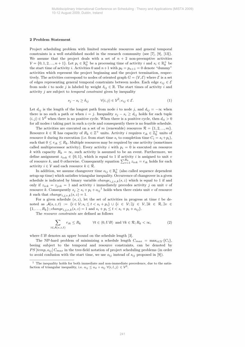
2 Problem Statement

Project scheduling problem with limited renewable resources and general temporal

constraints is a well established model in the research community (see [7], [9], [13]).

We assume that the project deals with a set of n + 2 non-preemptive activities

V = {0, 1, 2, ..., n + 1}. Let pi ∈ R+0

be a processing time of activity i and si ∈ R+0

be

the start time of activity i. Activities 0 and n+1 with p0 = pn+1 = 0 denote “dummy”

activities which represent the project beginning and the project termination, respec-

tively. The activities correspond to nodes of oriented graph G = (V, E) where E is a set

of edges representing general temporal constraints between nodes. Each edge eij ∈ E

from node i to node j is labeled by weight δij ∈ R. The start times of activity i and

activity j are subject to temporal constraint given by inequality

sj − si ≥ δij ∀(i, j) ∈ V2; eij ∈ E . (1)

Let dij is the length of the longest path from node i to node j, and dij = −∞ when

there is no such a path or when i = j. Inequality sj − si ≥ dij holds for each tuple

(i, j) ∈ V2 when there is no positive cycle. When there is a positive cycle, then dii > 0

for all nodes i taking part in such a cycle and consequently there is no feasible schedule.

The activities are executed on a set of m (renewable) resources R = {1, 2, ..., m}.

Resource k ∈ R has capacity of Rk ∈ Z+ units. Activity i requires rik ∈ Z

+0

units of

resource k during its execution (i.e. from start time si to completion time Ci = si +pi),

such that 0 ≤ rik ≤ Rk. Multiple resources may be required by one activity (sometimes

called multiprocessor activity). Every activity i with pi = 0 is executed on resource

k with capacity Rk = ∞, such activity is assumed to be an event. Furthermore, we

define assignment zivk ∈ {0, 1}, which is equal to 1 if activity i is assigned to unit v

of resource k, and 0 otherwise. Consequently equation∑Rk

v=1zivk = rik holds for each

activity i ∈ V and each resource k ∈ R.

In addition, we assume changeover time oij ∈ R+0

(also called sequence dependent

setup-up time) which satisfies triangular inequality. Occurrence of changeover in a given

schedule is indicated by binary variable changei,j,v,k(s, z) which is equal to 1 if and

only if zivk = zjvk = 1 and activity i immediately precedes activity j on unit v of

resource k. Consequently sj ≥ si + pi + oij1 holds when there exists unit v of resource

k such that changei,j,v,k(s, z) = 1.

For a given schedule (s, z), let the set of activities in progress at time t be de-

noted as A(s, z, t) := {i ∈ V; si ≤ t < si + pi} ∪ {i ∈ V; ∃j ∈ V, ∃k ∈ R,∃v ∈

{1, . . . , Rk} ; changei,j,v,k(s, z) = 1 and si + pi ≤ t < si + pi + oij}.

The resource constraints are defined as follows∑i∈A(s,z,t)

rik ≤ Rk ∀t ∈ 〈0, UB〉 and ∀k ∈ R; Rk < ∞, (2)

where UB denotes an upper bound on the schedule length [3].

The NP-hard problem of minimizing a schedule length Cmax = maxi∈V {Ci},

beeing subject to the temporal and resource constraints, can be denoted by

PS∣∣temp, oij

∣∣ Cmax in the tree-field notation of project scheduling problems (in order

to avoid confusion with the start time, we use oij instead of sij proposed in [9]).

1 The inequality holds for both immediate and non-immediate precedence, due to the satis-faction of triangular inequality, i.e. oij ≤ oil + olj ∀(i, l, j) ∈ V3.


241

We extend this problem by a concept of take-give resources as follows. Let us

assume a set of b take-give resources Q = {1, 2, ..., b}. Take-give resource k ∈ Q has

capacity of Qk ∈ Z+ units such that Qk < ∞. Analogously to activity executed

on resources, we introduce occupation executed on take-give resources. Occupation i

requires ailk ∈ {0, 1} units of take-give resource k ∈ Q during its execution. Occupation

i starts its execution at si, start time of activity which takes a take-give resource, and

finishes its execution at Cl = sl + pl, completion time of activity which gives back (i.e.

releases) the take-give resource. Multiple take-give resources may be taken or given

back by one activity, but there is at most one take-give resource taken by activity i

and given back by activity l (i.e.∑

k∈Q ailk ≤ 1 ∀(i, l) ∈ V2) and there is a path from

i to l with dil > 0. We define take-give assignment zivk ∈ {0, 1}, which is equal to 1 if

occupation i is assigned to unit v of take-give resource k, and 0 otherwise. Consequently

equation∑Qk

v=1zivk = ailk holds for each (i, l) ∈ V2 and each resource k ∈ Q.

In the same way, as for resources, we assume changeover time oij ∈ R+0

on take-give

resources which also satisfies triangular inequality. Occurrence of changeover in a given

schedule is indicated by binary variable ˜changei,j,v,k(s, z) which is equal to 1 if and

only if zivk = zjvk = 1 and occupation i immediately precedes occupation j on unit v

of take-give resource k. Consequently sj ≥ sl + pl + oij holds when there exists unit v

of resource k such that ˜changei,j,v,k(s, z) = 1.

For a given schedule (s, z), let the set of occupations in progress at time t is denoted

as O(s, t, z) := {(i, l) ∈ V2; ∃k ∈ Q, ailk = 1, si ≤ t < sl + pl} ∪ {i ∈ V; ∃j ∈ V, ∃k ∈

Q, ∃v ∈ {1, . . . , Qk} , ˜changei,j,v,k(s, z) = 1 and si + pi ≤ t < sl + pl + oij}. The

take-give resource constraints are as follows:∑(i,l)∈O(s,t)

ailk ≤ Qk ∀t ∈ 〈0, UB〉 and ∀k ∈ Q. (3)

A schedule S = (s, z, z) is feasible if it satisfies the temporal, resource and take-

give resource constraints. A set of feasible schedules for given input data is denoted by

S. The problem of finding a feasible schedule with minimal Cmax can be denoted by

PS∣∣temp, oij , tg

∣∣ Cmax.

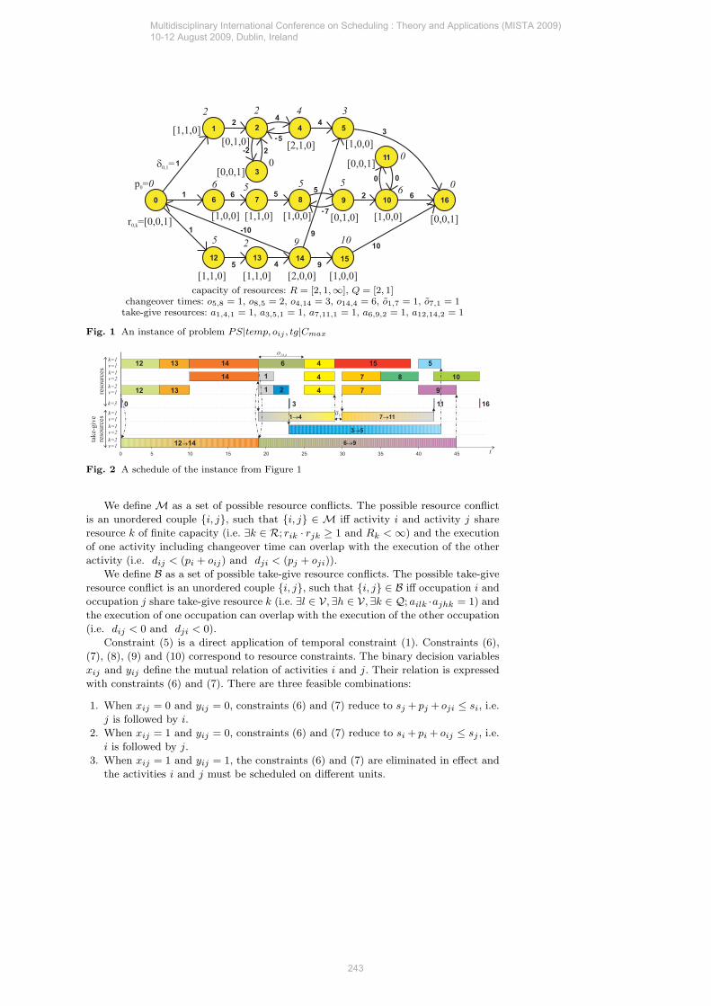
An instance of problem PS|temp, oij , tg|Cmax is shown in Figure 1. The example

considers 3 resources and 2 take-give resources with different capacities. There are 5

occupations, e.g. activity 12 takes resource 2 at its start time and at the completion

time of activity 14 the resource is given-back. On the other hand, if we need to bind a

resource taking with the completion time of an activity we could model it as it is shown

in the figure on activities 2 and 3. The start time of dummy activity 3 is synchronized

with the completion time of activity 2 by edges e2,3 and e3,2. Therefore occupation 3

can be seen as an occupation taken at the completion time of activity 2. In the same

way, resource giving-back can be bind with start time of an activity as is shown in the

figure on activities 10, 11. A schedule of this instance is shown in Figure 2.

3 Integer Linear Programming Formulation

In this part, we define problem PS|temp, oij , tg|Cmax by Integer Linear Programming.

Let xij be a binary decision variable such that xij = 1 if and only if i is followed by

j and xij = 0 if and only if j is followed by i. Furthermore, let yij be another binary

decision variable such that if yij = 1 the resource constraints are eliminated in effect,

i.e. activities i and j can not share an unit.


242

r =0,k [0,0,1]

[1,1,0][0,1,0]

[0,0,1]

[2,1,0] [1,0,0]

[1,0,0] [1,1,0] [1,0,0] [0,1,0] [1,0,0]

[1,1,0] [1,1,0] [2,0,0] [1,0,0]

[0,0,1]

p =0 0

2 2

0

4 3

6 5 5 56

0

0

5 2 9 10

[0,0,1]0 0

d0,1=

capacity of resources: R = [2, 1,∞], Q = [2, 1]changeover times: o5,8 = 1, o8,5 = 2, o4,14 = 3, o14,4 = 6, o1,7 = 1, o7,1 = 1

take-give resources: a1,4,1 = 1, a3,5,1 = 1, a7,11,1 = 1, a6,9,2 = 1, a12,14,2 = 1

Fig. 1 An instance of problem PS|temp, oij , tg|Cmax

12 14® 6 9®

3 5®

1 4® 7 11®

12

12

13

13

14

14 1

1 2

4

4

4

3

7

7 8

15 5

10

9

0 11 16

6

t

k=1v=1

k=1v=2

k=2v=1

k=3

k=1v=1

k=1v=2

k=2v=1

reso

urc

es

take-

giv

ere

sourc

es

o17~

o14,4

Fig. 2 A schedule of the instance from Figure 1

We define M as a set of possible resource conflicts. The possible resource conflict

is an unordered couple {i, j}, such that {i, j} ∈ M iff activity i and activity j share

resource k of finite capacity (i.e. ∃k ∈ R; rik · rjk ≥ 1 and Rk < ∞) and the execution

of one activity including changeover time can overlap with the execution of the other

activity (i.e. dij < (pi + oij) and dji < (pj + oji)).

We define B as a set of possible take-give resource conflicts. The possible take-give

resource conflict is an unordered couple {i, j}, such that {i, j} ∈ B iff occupation i and

occupation j share take-give resource k (i.e. ∃l ∈ V, ∃h ∈ V, ∃k ∈ Q; ailk ·ajhk = 1) and

the execution of one occupation can overlap with the execution of the other occupation

(i.e. dij < 0 and dji < 0).

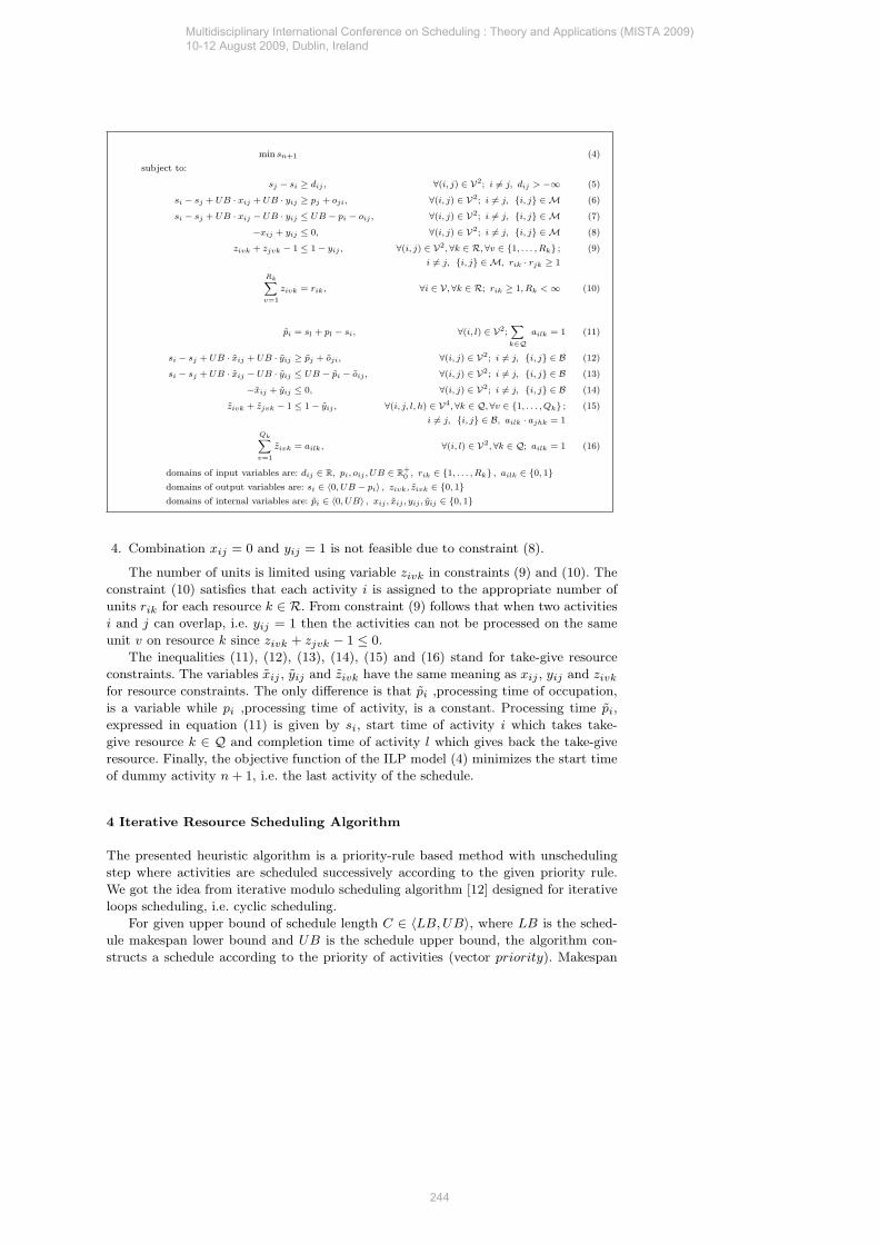
Constraint (5) is a direct application of temporal constraint (1). Constraints (6),

(7), (8), (9) and (10) correspond to resource constraints. The binary decision variables

xij and yij define the mutual relation of activities i and j. Their relation is expressed

with constraints (6) and (7). There are three feasible combinations:

1. When xij = 0 and yij = 0, constraints (6) and (7) reduce to sj + pj + oji ≤ si, i.e.

j is followed by i.

2. When xij = 1 and yij = 0, constraints (6) and (7) reduce to si + pi + oij ≤ sj , i.e.

i is followed by j.

3. When xij = 1 and yij = 1, the constraints (6) and (7) are eliminated in effect and

the activities i and j must be scheduled on different units.


243

min sn+1 (4)

subject to:

sj − si ≥ dij , ∀(i, j) ∈ V2; i 6= j, dij > −∞ (5)

si − sj + UB · xij + UB · yij ≥ pj + oji, ∀(i, j) ∈ V2; i 6= j, {i, j} ∈ M (6)

si − sj + UB · xij − UB · yij ≤ UB − pi − oij , ∀(i, j) ∈ V2; i 6= j, {i, j} ∈ M (7)

−xij + yij ≤ 0, ∀(i, j) ∈ V2; i 6= j, {i, j} ∈ M (8)

zivk + zjvk − 1 ≤ 1 − yij , ∀(i, j) ∈ V2,∀k ∈ R, ∀v ∈ {1, . . . , Rk} ; (9)

i 6= j, {i, j} ∈ M, rik · rjk ≥ 1

Rk∑v=1

zivk = rik, ∀i ∈ V,∀k ∈ R; rik ≥ 1, Rk < ∞ (10)

pi = sl + pl − si, ∀(i, l) ∈ V2;∑k∈Q

ailk = 1 (11)

si − sj + UB · xij + UB · yij ≥ pj + oji, ∀(i, j) ∈ V2; i 6= j, {i, j} ∈ B (12)

si − sj + UB · xij − UB · yij ≤ UB − pi − oij , ∀(i, j) ∈ V2; i 6= j, {i, j} ∈ B (13)

−xij + yij ≤ 0, ∀(i, j) ∈ V2; i 6= j, {i, j} ∈ B (14)

zivk + zjvk − 1 ≤ 1 − yij , ∀(i, j, l, h) ∈ V4, ∀k ∈ Q, ∀v ∈ {1, . . . , Qk} ; (15)

i 6= j, {i, j} ∈ B, ailk · ajhk = 1

Qk∑v=1

zivk = ailk, ∀(i, l) ∈ V2,∀k ∈ Q; ailk = 1 (16)

domains of input variables are: dij ∈ R, pi, oij , UB ∈ R+

0, rik ∈ {1, . . . , Rk} , ailk ∈ {0, 1}

domains of output variables are: si ∈ 〈0, UB − pi〉 , zivk, zivk ∈ {0, 1}

domains of internal variables are: pi ∈ 〈0, UB〉 , xij , xij , yij , yij ∈ {0, 1}

4. Combination xij = 0 and yij = 1 is not feasible due to constraint (8).

The number of units is limited using variable zivk in constraints (9) and (10). The

constraint (10) satisfies that each activity i is assigned to the appropriate number of

units rik for each resource k ∈ R. From constraint (9) follows that when two activities

i and j can overlap, i.e. yij = 1 then the activities can not be processed on the same

unit v on resource k since zivk + zjvk − 1 ≤ 0.

The inequalities (11), (12), (13), (14), (15) and (16) stand for take-give resource

constraints. The variables xij , yij and zivk have the same meaning as xij , yij and zivk

for resource constraints. The only difference is that pi ,processing time of occupation,

is a variable while pi ,processing time of activity, is a constant. Processing time pi,

expressed in equation (11) is given by si, start time of activity i which takes take-

give resource k ∈ Q and completion time of activity l which gives back the take-give

resource. Finally, the objective function of the ILP model (4) minimizes the start time

of dummy activity n + 1, i.e. the last activity of the schedule.

4 Iterative Resource Scheduling Algorithm

The presented heuristic algorithm is a priority-rule based method with unscheduling

step where activities are scheduled successively according to the given priority rule.

We got the idea from iterative modulo scheduling algorithm [12] designed for iterative

loops scheduling, i.e. cyclic scheduling.

For given upper bound of schedule length C ∈ 〈LB, UB〉, where LB is the sched-

ule makespan lower bound and UB is the schedule upper bound, the algorithm con-

structs a schedule according to the priority of activities (vector priority). Makespan


244

bounds LB and UB are initialized in the same way as is described in [3]. Function

findSchedule(C, priority, budget) tries to find a feasible schedule with Cmax ≤ C while

the number of scheduling steps is limited by budget = n · budgetRatio. The algorithm

parameter BudgetRatio is the ratio of the maximum number of activity scheduling

steps to the number of activities n.

If function findSchedule finds a feasible schedule S, activities are shifted to the left

side in function shiftLeft(S) so that constraints and order of activities in S is kept. In

other words, this operation finds optimal schedule Sleft for order of activities given

by S using the longest paths evaluation. Furthermore, the improved schedule Sleft is

used to update upper bound UB = Cmax(Sleft) − 1. On the other hand, if function

findSchedule(C, priority, budget) can not find a feasible schedule within the given limit

of scheduling steps (i.e. budget) the schedule lower bound is increased LB = C+1. The

best solution Sbest with respect to Cmax is searched using interval bisection method

over C ∈ 〈LB, UB〉.

input : an instance PS|temp, oij , tg|Cmax, budgetRatio

output: schedule Sbest.

Calculate di,j ∀(i, j) ∈ V2;

Calculate LB and UB;

C = LB; Sbest = {};

budget = budgetRatio · n;

priority(i) = di,n+1;

while LB ≤ UB do

S = findSchedule(C, priority, budget);

if S is feasible then

Sleft = shiftLeft(S);

UB = Cmax(Sleft) − 1; Sbest = Sleft;

else

LB = C + 1;

end

C = ⌈(LB + UB)/2⌉;

end

Algorithm 1: Iterative Resource Scheduling algorithm

Function findSchedule(C, priority, budget) constructs a schedule with Cmax ≤ C

using vector of priorities priority. As a priority we use the longest path from activity i

to activity n+1, i.e. priorityi = di,n+1. Until a feasible schedule is not found or upper

bound of scheduling steps budget is not reached, the function choses such activity i with

highest priority which was not scheduled yet. Subsequently, the algorithm determines

the earliest and latest start time of the activity ESi and LSi respectively. Then function

findTimeSlot(i, ESi, LSi) finds the first si ∈ 〈ESi, LSi〉 such that there are no conflicts

on resources R,Q. If there is no such si then si is determined according to whether

activity i was scheduled once. If the activity is being scheduled for the first time,

then si = ESi otherwise si = sprevi + 1 where sprev

i is the previous start time. Finally,


245

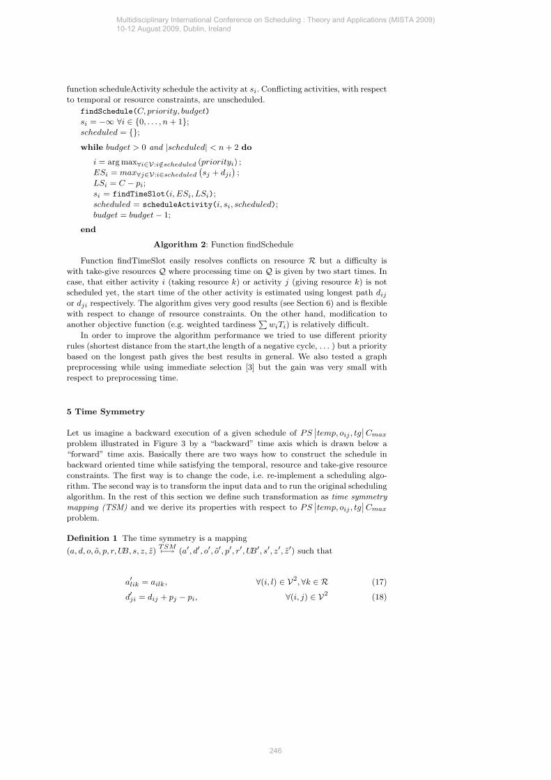
function scheduleActivity schedule the activity at si. Conflicting activities, with respect

to temporal or resource constraints, are unscheduled.

findSchedule(C, priority, budget)

si = −∞ ∀i ∈ {0, . . . , n + 1};

scheduled = {};

while budget > 0 and |scheduled| < n + 2 do

i = arg max∀i∈V:i/∈scheduled (priorityi) ;

ESi = max∀j∈V:i∈scheduled

(sj + dji

);

LSi = C − pi;

si = findTimeSlot(i, ESi, LSi);

scheduled = scheduleActivity(i, si, scheduled);

budget = budget − 1;

end

Algorithm 2: Function findSchedule

Function findTimeSlot easily resolves conflicts on resource R but a difficulty is

with take-give resources Q where processing time on Q is given by two start times. In

case, that either activity i (taking resource k) or activity j (giving resource k) is not

scheduled yet, the start time of the other activity is estimated using longest path dij

or dji respectively. The algorithm gives very good results (see Section 6) and is flexible

with respect to change of resource constraints. On the other hand, modification to

another objective function (e.g. weighted tardiness∑

wiTi) is relatively difficult.

In order to improve the algorithm performance we tried to use different priority

rules (shortest distance from the start,the length of a negative cycle, . . . ) but a priority

based on the longest path gives the best results in general. We also tested a graph

preprocessing while using immediate selection [3] but the gain was very small with

respect to preprocessing time.

5 Time Symmetry

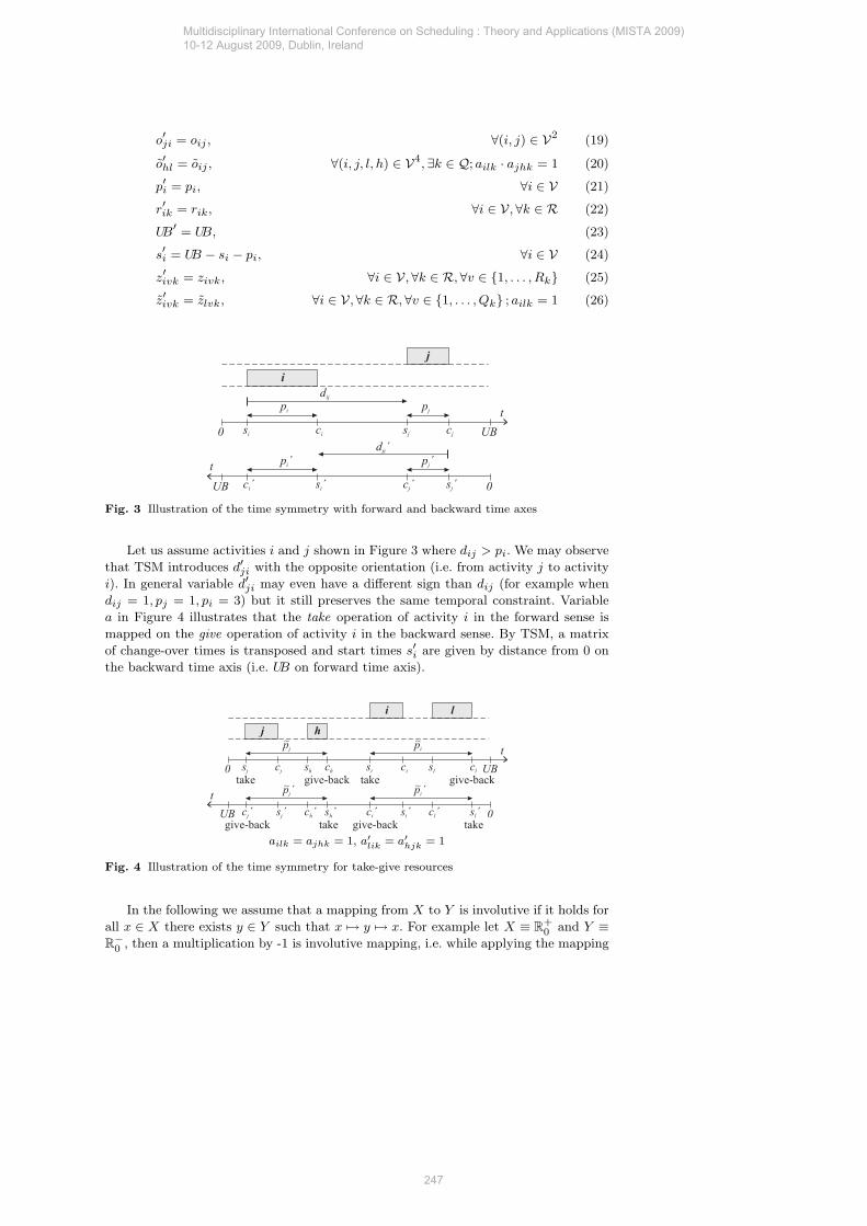
Let us imagine a backward execution of a given schedule of PS∣∣temp, oij , tg

∣∣ Cmax

problem illustrated in Figure 3 by a “backward” time axis which is drawn below a

“forward” time axis. Basically there are two ways how to construct the schedule in

backward oriented time while satisfying the temporal, resource and take-give resource

constraints. The first way is to change the code, i.e. re-implement a scheduling algo-

rithm. The second way is to transform the input data and to run the original scheduling

algorithm. In the rest of this section we define such transformation as time symmetry

mapping (TSM) and we derive its properties with respect to PS∣∣temp, oij , tg

∣∣ Cmax

problem.

Definition 1 The time symmetry is a mapping

(a, d, o, o, p, r, UB, s, z, z)TSM7−→ (a′, d′, o′, o′, p′, r′, UB′, s′, z′, z′) such that

a′lik = ailk, ∀(i, l) ∈ V2, ∀k ∈ R (17)

d′ji = dij + pj − pi, ∀(i, j) ∈ V2 (18)


246

o′ji = oij , ∀(i, j) ∈ V2 (19)

o′hl = oij , ∀(i, j, l, h) ∈ V4, ∃k ∈ Q; ailk · ajhk = 1 (20)

p′i = pi, ∀i ∈ V (21)

r′ik = rik, ∀i ∈ V, ∀k ∈ R (22)

UB′ = UB, (23)

s′i = UB − si − pi, ∀i ∈ V (24)

z′ivk = zivk, ∀i ∈ V, ∀k ∈ R, ∀v ∈ {1, . . . , Rk} (25)

z′ivk = zlvk, ∀i ∈ V, ∀k ∈ R, ∀v ∈ {1, . . . , Qk} ; ailk = 1 (26)

si ci sj cj

pi

i

j

dij

pj

ci´ s ´i cj´ sj´

pi´

dji´

pj´

0

UB 0

UB

t

t

Fig. 3 Illustration of the time symmetry with forward and backward time axes

Let us assume activities i and j shown in Figure 3 where dij > pi. We may observe

that TSM introduces d′ji with the opposite orientation (i.e. from activity j to activity

i). In general variable d′ji may even have a different sign than dij (for example when

dij = 1, pj = 1, pi = 3) but it still preserves the same temporal constraint. Variable

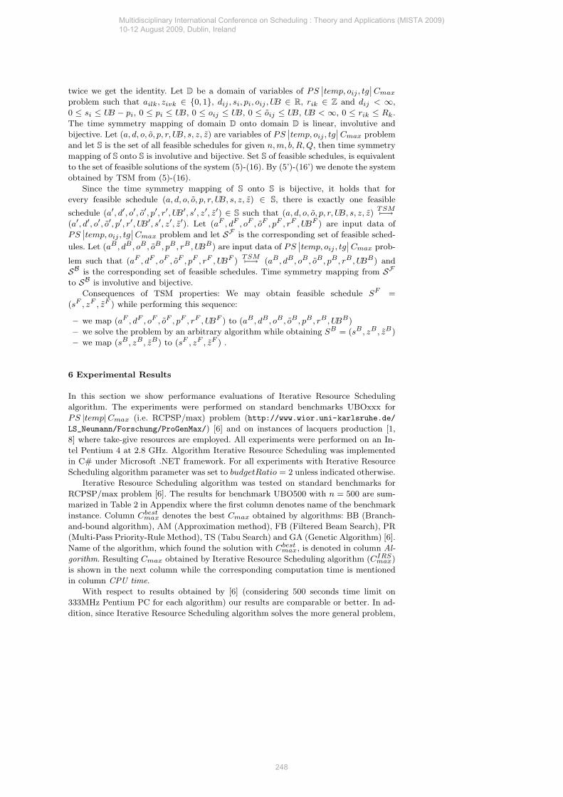
a in Figure 4 illustrates that the take operation of activity i in the forward sense is

mapped on the give operation of activity i in the backward sense. By TSM, a matrix

of change-over times is transposed and start times s′i are given by distance from 0 on

the backward time axis (i.e. UB on forward time axis).

si ci sl cl

i l

ci´ s ´i cl´ sl´

0

UB 0

UB

t

t

sj

pj

sh ch

cj´ s ´j ch´ sh´

j h~ pi

~

pj´~ pi´

~

cj

takegive-backtakegive-back

take give-backtake give-back

ailk = ajhk = 1, a′

lik= a′

hjk= 1

Fig. 4 Illustration of the time symmetry for take-give resources

In the following we assume that a mapping from X to Y is involutive if it holds for

all x ∈ X there exists y ∈ Y such that x 7→ y 7→ x. For example let X ≡ R+0

and Y ≡

R−0

, then a multiplication by -1 is involutive mapping, i.e. while applying the mapping


247

twice we get the identity. Let D be a domain of variables of PS∣∣temp, oij , tg

∣∣ Cmax

problem such that ailk, zivk ∈ {0, 1}, dij , si, pi, oij , UB ∈ R, rik ∈ Z and dij < ∞,

0 ≤ si ≤ UB − pi, 0 ≤ pi ≤ UB, 0 ≤ oij ≤ UB, 0 ≤ oij ≤ UB, UB < ∞, 0 ≤ rik ≤ Rk.

The time symmetry mapping of domain D onto domain D is linear, involutive and

bijective. Let (a, d, o, o, p, r, UB, s, z, z) are variables of PS∣∣temp, oij , tg

∣∣ Cmax problem

and let S is the set of all feasible schedules for given n, m, b, R, Q, then time symmetry

mapping of S onto S is involutive and bijective. Set S of feasible schedules, is equivalent

to the set of feasible solutions of the system (5)-(16). By (5’)-(16’) we denote the system

obtained by TSM from (5)-(16).

Since the time symmetry mapping of S onto S is bijective, it holds that for

every feasible schedule (a, d, o, o, p, r, UB, s, z, z) ∈ S, there is exactly one feasible

schedule (a′, d′, o′, o′, p′, r′, UB′, s′, z′, z′) ∈ S such that (a, d, o, o, p, r, UB, s, z, z)TSM7−→

(a′, d′, o′, o′, p′, r′, UB′, s′, z′, z′). Let (aF , dF , oF , oF , pF , rF , UBF ) are input data of

PS∣∣temp, oij , tg

∣∣ Cmax problem and let SF is the corresponding set of feasible sched-

ules. Let (aB , dB , oB , oB , pB , rB , UBB) are input data of PS∣∣temp, oij , tg

∣∣ Cmax prob-

lem such that (aF , dF , oF , oF , pF , rF , UBF )TSM7−→ (aB , dB , oB , oB , pB , rB , UBB) and

SB is the corresponding set of feasible schedules. Time symmetry mapping from SF

to SB is involutive and bijective.

Consequences of TSM properties: We may obtain feasible schedule SF =

(sF , zF , zF ) while performing this sequence:

– we map (aF , dF , oF , oF , pF , rF , UBF ) to (aB , dB , oB , oB , pB , rB , UBB)

– we solve the problem by an arbitrary algorithm while obtaining SB = (sB , zB , zB)

– we map (sB , zB , zB) to (sF , zF , zF ) .

6 Experimental Results

In this section we show performance evaluations of Iterative Resource Scheduling

algorithm. The experiments were performed on standard benchmarks UBOxxx for

PS |temp|Cmax (i.e. RCPSP/max) problem (http://www.wior.uni-karlsruhe.de/

LS_Neumann/Forschung/ProGenMax/) [6] and on instances of lacquers production [1,

8] where take-give resources are employed. All experiments were performed on an In-

tel Pentium 4 at 2.8 GHz. Algorithm Iterative Resource Scheduling was implemented

in C# under Microsoft .NET framework. For all experiments with Iterative Resource

Scheduling algorithm parameter was set to budgetRatio = 2 unless indicated otherwise.

Iterative Resource Scheduling algorithm was tested on standard benchmarks for

RCPSP/max problem [6]. The results for benchmark UBO500 with n = 500 are sum-

marized in Table 2 in Appendix where the first column denotes name of the benchmark

instance. Column Cbestmax denotes the best Cmax obtained by algorithms: BB (Branch-

and-bound algorithm), AM (Approximation method), FB (Filtered Beam Search), PR

(Multi-Pass Priority-Rule Method), TS (Tabu Search) and GA (Genetic Algorithm) [6].

Name of the algorithm, which found the solution with Cbestmax, is denoted in column Al-

gorithm. Resulting Cmax obtained by Iterative Resource Scheduling algorithm (CIRSmax)

is shown in the next column while the corresponding computation time is mentioned

in column CPU time.

With respect to results obtained by [6] (considering 500 seconds time limit on

333MHz Pentium PC for each algorithm) our results are comparable or better. In ad-

dition, since Iterative Resource Scheduling algorithm solves the more general problem,


248

http://www.wior.uni-karlsruhe.de/LS_Neumann/Forschung/ProGenMax/

http://www.wior.uni-karlsruhe.de/LS_Neumann/Forschung/ProGenMax/

Instance Orders nFbudgetRatio = 2

FbudgetRatio = 4

BbudgetRatio = 2

met bro uniCmax

[-]CPU

time [s]Cmax

[-]CPU

time [s]Cmax

[-]CPU

time [s]

lacquery-1-01.ins 7 8 7 170 73681 3.58 73681 9.66 71435 13.31lacquery-1-02.ins 8 8 7 176 77449 3.92 77449 10.41 75203 15.56lacquery-1-03.ins 8 7 8 175 68313 4.77 68683 13.16 73432 11.66lacquery-1-04.ins 7 8 8 178 74455 3.88 74455 9.61 72231 13.91lacquery-1-05.ins 8 8 8 184 78223 4.72 78223 12.09 75999 16.36lacquery-1-06.ins 9 8 8 190 81991 5.59 81991 14.31 81169 17.08lacquery-1-07.ins 8 9 8 193 77594 2.67 77594 6.39 84621 16.08lacquery-1-08.ins 8 8 9 192 78688 5.36 78688 14.80 77180 12.99lacquery-1-09.ins 9 9 8 199 85718 6.94 81362 9.55 88389 18.940lacquery-1-10.ins 9 8 9 198 82456 6.30 82456 17.20 80948 15.61lacquery-1-11.ins 8 9 9 201 81950 6.360 81950 21.70 81866 16.88lacquery-1-12.ins 9 9 9 207 85718 7.58 85718 25.05 85634 19.38lacquery-1-13.ins 10 9 9 213 89486 9.03 89486 30.4 89402 21.59lacquery-1-14.ins 9 10 9 216 90539 8.95 86409 15.00 90671 35.69lacquery-1-15.ins 9 9 10 215 87844 8.02 87844 25.25 89316 22.24lacquery-1-16.ins 10 10 9 222 94307 10.56 90177 19.55 94439 40.25lacquery-1-17.ins 10 9 10 221 91612 9.19 91612 24.39 93084 26.11lacquery-1-18.ins 9 10 10 224 90798 8.11 90798 20.31 92462 25.49lacquery-1-19.ins 10 10 10 230 94566 9.92 94566 24.86 96230 28.45

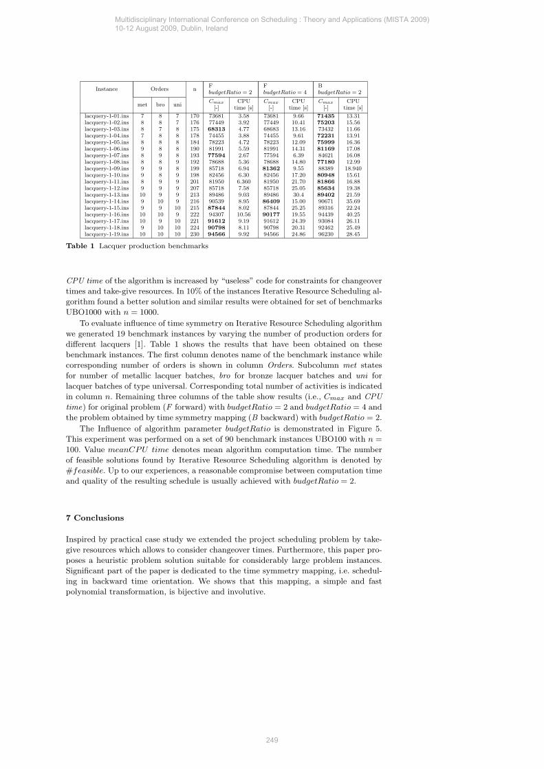
Table 1 Lacquer production benchmarks

CPU time of the algorithm is increased by “useless” code for constraints for changeover

times and take-give resources. In 10% of the instances Iterative Resource Scheduling al-

gorithm found a better solution and similar results were obtained for set of benchmarks

UBO1000 with n = 1000.

To evaluate influence of time symmetry on Iterative Resource Scheduling algorithm

we generated 19 benchmark instances by varying the number of production orders for

different lacquers [1]. Table 1 shows the results that have been obtained on these

benchmark instances. The first column denotes name of the benchmark instance while

corresponding number of orders is shown in column Orders. Subcolumn met states

for number of metallic lacquer batches, bro for bronze lacquer batches and uni for

lacquer batches of type universal. Corresponding total number of activities is indicated

in column n. Remaining three columns of the table show results (i.e., Cmax and CPU

time) for original problem (F forward) with budgetRatio = 2 and budgetRatio = 4 and

the problem obtained by time symmetry mapping (B backward) with budgetRatio = 2.

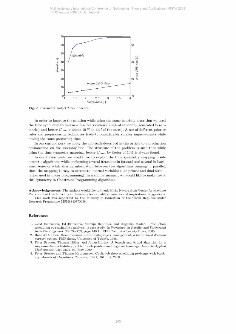
The Influence of algorithm parameter budgetRatio is demonstrated in Figure 5.

This experiment was performed on a set of 90 benchmark instances UBO100 with n =

100. Value meanCPU time denotes mean algorithm computation time. The number

of feasible solutions found by Iterative Resource Scheduling algorithm is denoted by

#feasible. Up to our experiences, a reasonable compromise between computation time

and quality of the resulting schedule is usually achieved with budgetRatio = 2.

7 Conclusions

Inspired by practical case study we extended the project scheduling problem by take-

give resources which allows to consider changeover times. Furthermore, this paper pro-

poses a heuristic problem solution suitable for considerably large problem instances.

Significant part of the paper is dedicated to the time symmetry mapping, i.e. schedul-

ing in backward time orientation. We shows that this mapping, a simple and fast

polynomial transformation, is bijective and involutive.


249

budgetRatio [-]

#fe

asi

ble

[-]

mean CPU time

#feasible

mea

n C

PU

tim

e[s

]

Fig. 5 Parameter budgetRatio influence

In order to improve the solution while using the same heuristic algorithm we used

the time symmetry to find new feasible solution (in 4% of randomly generated bench-

marks) and better Cmax ( about 10 % in half of the cases). A use of different priority

rules and preprocessing techniques leads to considerably smaller improvements while

having the same processing time.

In our current work we apply the approach described in this article to a production

optimization on the assembly line. The structure of the problem is such that while

using the time symmetry mapping, better Cmax by factor of 10% is always found.

In our future work, we would like to exploit the time symmetry mapping inside

heuristic algorithms while performing several iterations in forward and several in back-

ward sense or while sharing information between two algorithms running in parallel,

since the mapping is easy to extend to internal variables (like primal and dual formu-

lation used in linear programming). In a similar manner, we would like to make use of

this symmetry in Constraint Programming algorithms.

Acknowledgements The authors would like to thank Mirko Navara from Center for MachinePerception at Czech Technical University for valuable comments and inspirational suggestions.

This work was supported by the Ministry of Education of the Czech Republic underResearch Programme MSM6840770038.

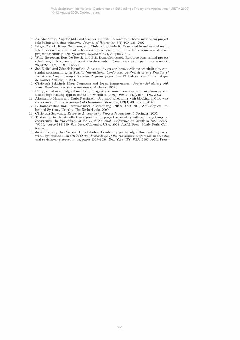
References

1. Gerd Behrmann, Ed Brinksma, Martijn Hendriks, and Angelika Mader. Productionscheduling by reachability analysis - a case study. In Workshop on Parallel and Distributed

Real-Time Systems (WPDRTS), page 140.1. IEEE Computer Society Press, 2005.2. Ronald De Boer. Resource-constrained multi-project management, a hierarchical decision

support system. PhD thesis, University of Twente, 1998.3. Peter Brucker, Thomas Hilbig, and Johan Hurink. A branch and bound algorithm for a

single-machine scheduling problem with positive and negative time-lags. Discrete Applied

Mathematics, 94(1-3):77–99, May 1999.4. Peter Brucker and Thomas Kampmeyer. Cyclic job shop scheduling problems with block-

ing. Annals of Operations Research, 159(1):161–181, 2008.


250

5. Amedeo Cesta, Angelo Oddi, and Stephen F. Smith. A constraint-based method for projectscheduling with time windows. Journal of Heuristics, 8(1):109–136, 2002.

6. Birger Franck, Klaus Neumann, and Christoph Schwindt. Truncated branch–and–bound,schedule-construction, and schedule-improvement procedures for resource-constrainedproject scheduling. OR Spektrum, 23(3):297–324, August 2001.

7. Willy Herroelen, Bert De Reyck, and Erik Demeulemeester. Resource-constrained projectscheduling : A survey of recent developments. Computers and operations research,25(4):279–302, 1998. Elsevier.

8. Jan Kelbel and Zdenek Hanzalek. A case study on earliness/tardiness scheduling by con-straint programming. In Twelfth International Conference on Principles and Practice of

Constraint Programming - Doctoral Program, pages 108–113. Laboratoire DInformatiquede Nantes Atlantique, 2006.

9. Christoph Schwindt Klaus Neumann and Jrgen Zimmermann. Project Scheduling with

Time Windows and Scarce Resources. Springer, 2003.10. Philippe Laborie. Algorithms for propagating resource constraints in ai planning and

scheduling: existing approaches and new results. Artif. Intell., 143(2):151–188, 2003.11. Alessandro Mascis and Dario Pacciarelli. Job-shop scheduling with blocking and no-wait

constraints. European Journal of Operational Research, 143(3):498 – 517, 2002.12. B. Ramakrishna Rau. Iterative modulo scheduling. PROGRESS 2000 Workshop on Em-

bedded Systems, Utrecht, The Netherlands, 2000.13. Christoph Schwindt. Resource Allocation in Project Management. Springer, 2005.14. Tristan B. Smith. An effective algorithm for project scheduling with arbitrary temporal

constraints. In Proceedings of the 19 th National Conference on Artificial Intelligence.

(2004), pages 544–549, San Jose, California, USA, 2004. AAAI Press, Menlo Park, Cali-fornia.

15. Justin Terada, Hoa Vo, and David Joslin. Combining genetic algorithms with squeaky-wheel optimization. In GECCO ’06: Proceedings of the 8th annual conference on Genetic

and evolutionary computation, pages 1329–1336, New York, NY, USA, 2006. ACM Press.


251

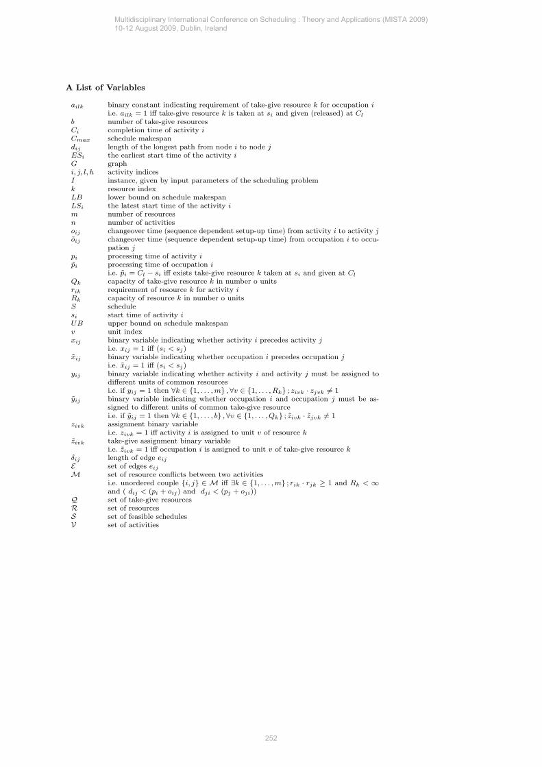
A List of Variables

ailk binary constant indicating requirement of take-give resource k for occupation i

i.e. ailk = 1 iff take-give resource k is taken at si and given (released) at Cl

b number of take-give resourcesCi completion time of activity i

Cmax schedule makespandij length of the longest path from node i to node j

ESi the earliest start time of the activity i

G graphi, j, l, h activity indicesI instance, given by input parameters of the scheduling problemk resource indexLB lower bound on schedule makespanLSi the latest start time of the activity i

m number of resourcesn number of activitiesoij changeover time (sequence dependent setup-up time) from activity i to activity j

oij changeover time (sequence dependent setup-up time) from occupation i to occu-pation j

pi processing time of activity i

pi processing time of occupation i

i.e. pi = Cl − si iff exists take-give resource k taken at si and given at Cl

Qk capacity of take-give resource k in number o unitsrik requirement of resource k for activity i

Rk capacity of resource k in number o unitsS schedulesi start time of activity i

UB upper bound on schedule makespanv unit indexxij binary variable indicating whether activity i precedes activity j

i.e. xij = 1 iff (si < sj)xij binary variable indicating whether occupation i precedes occupation j

i.e. xij = 1 iff (si < sj)yij binary variable indicating whether activity i and activity j must be assigned to

different units of common resourcesi.e. if yij = 1 then ∀k ∈ {1, . . . , m} , ∀v ∈ {1, . . . , Rk} ; zivk · zjvk 6= 1

yij binary variable indicating whether occupation i and occupation j must be as-signed to different units of common take-give resourcei.e. if yij = 1 then ∀k ∈ {1, . . . , b} , ∀v ∈ {1, . . . , Qk} ; zivk · zjvk 6= 1

zivk assignment binary variablei.e. zivk = 1 iff activity i is assigned to unit v of resource k

zivk take-give assignment binary variablei.e. zivk = 1 iff occupation i is assigned to unit v of take-give resource k

δij length of edge eij

E set of edges eij

M set of resource conflicts between two activitiesi.e. unordered couple {i, j} ∈ M iff ∃k ∈ {1, . . . , m} ; rik · rjk ≥ 1 and Rk < ∞and ( dij < (pi + oij) and dji < (pj + oji))

Q set of take-give resourcesR set of resourcesS set of feasible schedulesV set of activities


252

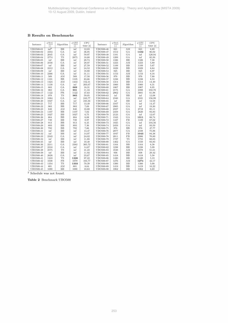
B Results on Benchmarks

InstanceCbest

max

[-]Algorithm

CIRS

max

[-]CPU

time [s]Instance

Cbest

max

[-]Algorithm

CIRS

max

[-]CPU

time [s]

UBO500-01 inf2 BB inf 12,03 UBO500-46 821 AM 821 6,89UBO500-02 2353 GA inf 36,05 UBO500-47 1512 GA 1432 86,02UBO500-03 2045 GA inf 59,97 UBO500-48 1181 GA inf 128,94UBO500-04 2774 TS 2875 18,80 UBO500-49 1209 GA inf 85,56UBO500-05 inf BB inf 20,74 UBO500-50 1326 BB 1326 7,38UBO500-06 2558 GA inf 29,97 UBO500-51 1223 AM 1223 5,89UBO500-07 inf BB inf 27,59 UBO500-52 1109 BB 1109 5,67UBO500-08 2212 GA inf 24,52 UBO500-53 1029 BB 1029 8,84UBO500-09 inf BB inf 18,80 UBO500-54 825 BB 825 6,97UBO500-10 2366 GA inf 31,11 UBO500-55 1153 AM 1153 6,16UBO500-11 589 AM 589 17,50 UBO500-56 976 BB 976 7,88UBO500-12 1101 BB 1105 83,66 UBO500-57 1238 BB 1238 8,53UBO500-13 1424 AM 1433 152,31 UBO500-58 1314 BB 1314 14,49UBO500-14 1130 GA inf 203,67 UBO500-59 1060 BB 1060 6,31UBO500-15 683 GA 669 18,31 UBO500-60 1067 BB 1067 8,95UBO500-16 982 GA 931 11,34 UBO500-61 2175 GA 2398 192,70UBO500-17 1122 PR 1122 47,63 UBO500-62 2962 GA 3601 61,98UBO500-18 978 TS 965 59,05 UBO500-63 inf BB inf 12,08UBO500-19 1084 GA inf 243,77 UBO500-64 2160 GA 2331 156,99UBO500-20 1027 GA inf 245,56 UBO500-65 inf BB inf 12,58UBO500-21 717 BB 717 13,49 UBO500-66 3167 GA inf 14,47UBO500-22 983 BB 983 7,69 UBO500-67 2905 GA inf 19,30UBO500-23 848 AM 848 10,80 UBO500-68 2337 GA 2718 85,11UBO500-24 1107 BB 1107 7,02 UBO500-69 2459 GA 2620 93,83UBO500-25 1027 BB 1027 6,75 UBO500-70 2123 GA inf 12,67UBO500-26 804 BB 804 6,08 UBO500-71 1343 GA 1311 88,74UBO500-27 749 BB 749 8,97 UBO500-72 1437 FB 1439 67,02UBO500-28 913 BB 913 6,45 UBO500-73 1925 GA inf 104,56UBO500-29 893 BB 893 7,36 UBO500-74 2459 GA inf 93,59UBO500-30 792 BB 792 7,66 UBO500-75 976 BB 976 47,77UBO500-31 inf BB inf 13,47 UBO500-76 2077 GA 2108 75,88UBO500-32 inf BB inf 14,97 UBO500-77 1047 FB 1043 84,38UBO500-33 2343 GA inf 24,02 UBO500-78 2011 FB 2086 70,89UBO500-34 inf BB inf 11,88 UBO500-79 1727 TS 1755 68,03UBO500-35 inf BB inf 10,48 UBO500-80 1462 GA 1550 83,83UBO500-36 2211 GA 2382 305,72 UBO500-81 1164 BB 1164 6,38UBO500-37 2318 GA inf 14,67 UBO500-82 1238 BB 1238 5,09UBO500-38 2575 TS inf 41,22 UBO500-83 1849 AM 1878 51,61UBO500-39 inf BB inf 11,92 UBO500-84 936 BB 938 29,42UBO500-40 2628 GA inf 23,67 UBO500-85 1418 BB 1418 5,58UBO500-41 1243 TS 1226 97,22 UBO500-86 1420 BB 1420 5,19UBO500-42 1038 FB 1079 103,77 UBO500-87 1276 AM 1274 42,17UBO500-43 1354 TS 1333 79,39 UBO500-88 1300 BB 1300 5,00UBO500-44 801 AM 801 8,64 UBO500-89 1419 BB 1419 16,22UBO500-45 1088 BB 1088 10,63 UBO500-90 1062 BB 1062 6,69

2 Schedule was not found.

Table 2 Benchmark UBO500


253

Documents

Time Symmetry of Project Scheduling with Time Windows …mistaconference.org/2009/papers/239-253-101-P.pdf · Time Symmetry of Project Scheduling with Time Windows and Take ... An