Time Varying Risk Return Relationship: Evidence from ... · PDF fileTime Varying Risk Return Relationship: Evidence from Listed Pakistani Firms 17 to-price ratio, book to market value

European Journal of Scientific Research ISSN 1450-216X Vol.22 No.1 (2008), pp.16-39 © EuroJournals Publishing, Inc. 2008 http://www.eurojournals.com/ejsr.htm

Time Varying Risk Return Relationship: Evidence from

Listed Pakistani Firms

Attiya Y. Javid Pakistan Institute of Development Economics, Islamabad, Pakistan

E-mail: [email protected] Tel: 92-51-9206616, Fax: 92-51-9210886

Abstract

This study empirically investigates the Fama-French three-factor model and consumption CAPM model in unconditional and conditional setting with individual stocks traded at Karachi Stock Exchange (KSE), the main equity market in Pakistan for the period 1993-2004. These extensions are in response of the empirical findings that do not support standard CAPM as a model to explain assets pricing in Pakistani equity market. The observation is that the dynamic size and book-to-market value coefficients explain the cross-section of expected returns in some sub-periods. In the second stage, the consumption risk is incorporated in standard CAPM in static and dynamic context. The findings reveal that the market rewards systematic risk for higher return, but the relevant measure for systematic risk appears to be conditional consumption beta rather than market beta. This evidence leads to investigate macroeconomic risks that can describe the variation in expected return in a more complete and meaningful way. Keywords: Capital asset pricing model, Fama-French Three-Factor model, market risk,

information set, business-cycle variables, consumption risk and market efficiency.

JEL Classification Codes: G11, G12, G15 1. Introduction The poor empirical response of the standard capital asset pricing model (CAPM) of Sharpe (1964) and Lintner (1965) may be due to the fact that the standard CAPM model assumes that the risk that an investors are concerned with the uncertainty about the future price of assets only. Investors however, are concerned with other risks that affect their ability to consume goods and services in future for example future relative price of consumer goods and future investment opportunities. Some researchers in financial economics have specified a number of possible factors that might explain the expected returns. This has led to the development of multifactor CAPM for example Arbitrage Pricing Theory (APT) of Ross (1976) and Intertemporal Asset Pricing Model (ICAPM) of Merton (1973) etc. These multifactor asset pricing model generalize the result of Sharpe-Lintner-Black model, and in these models risk is measured by covariance with several common factors in addition to market risk factor.

While specifying variables that are correlated with asset returns and testing whether the loadings of returns on these economic factors explain the cross-section of expected returns has motivated research in two directions. The first, initiated by Chen, Roll and Ross (1986), specifies macroeconomic variables that are thought to capture the systematic risks of the economy. A second method is to specify characteristics of the firm which are likely to explain the anomalies in asset returns. Some of such anomalies documented in literature are small firm effect, January effect, earning-

Time Varying Risk Return Relationship: Evidence from Listed Pakistani Firms 17

to-price ratio, book to market value and leverage etc. The most prominent work in this regard is series of papers by Fama and French, (1992, 1993, 1995, 1996, 1998 and 2004) 1, which construct hedge portfolios with long/short positions in firms with attributes known to be associated with mean returns. The three-factor model of Fama and French (1996) says that the expected returns in excess of risk free rate is explained by the (1) excess market return, (2) the difference between the returns on portfolio of small stocks and returns on portfolio of large stocks (SMB) and (3) the difference between the returns on portfolio of high book-to-market stocks and returns on a portfolio of low book-to-market stocks (HML). The three-factor model of Fama and French (1993) is now widely used in empirical research that requires a model of expected returns. Among practitioners, the model is offered as an alternative to the CAPM for estimating the cost of equity capital (for example, Ibbotson Associates) and portfolio performance [(Fama and French (2004)].

The joint nature of consumption decision and portfolio decision has also motivated research in comparing two formulations of capital asset pricing model, that is, the consumption CAPM and standard CAPM. Consumption-based model implies that, in equilibrium the prices of an asset equals the expected discounted value of future pay-offs, weighted by marginal utilities of consumption. The consumption beta appears preferable on theoretical grounds because it take account of intertemporal nature of portfolio decision [Merton (1973), Breeden (1979)] and because it implicitly incorporates many forms of wealth that are in principle relevant for measuring systematic risk. Merton (1973) has suggested that investor must be compensated in terms of expected returns for bearing the shift in opportunities set as well as taking on systematic market risk.

Another response is to incorporate conditioning information and motivates researcher to test condition asset pricing model. It is not reasonable to assume that investors live in one period and betas of assets remain constant, because investment decisions are made for many periods and the betas and expected returns generally depends on nature of information available at any point of time, and they vary over time as information set varies. We apply the conditional model in which the return distribution is time varying due to the change in the business conditions of the economy. Following Ferson and Harvey (1991, 1993 and 1999) and several other studies, we use the business cycle variables as information set. The relative risk of a firm cash flow is likely to vary over the business cycles. As Jagannathan and Wang (1996) have argued that to the extent that the business cycle is induced by technology and taste shocks, the relative shares of different sectors in the economy fluctuate, inducing fluctuations in the betas of the firms in these sectors. For example, the stocks of the poorly performing firms that are highly leveraged become more risky during recession. In bad times the risk premium is high because investors want to smooth out their consumption, therefore to make sure that investors hold their portfolio of stocks, the risk premium must be high in equilibrium. This line of argument implies that the instrument variables that are used for conditioning information must be related to current and future macroeconomic environment.

Extensive empirical work has been conducted for developed markets on conditional CAPM and conditional three factor model but very few studies have been done for emerging markets. The study by Iqbal and Brook (2007) have found evidence of non-linearity in the risk return relationship and come to the conclusion that for Pakistanis Stock market that the unconditional version of the CAPM is rejected. Iqbal et al. (2008) have tested CAPM and Fama and French (1993) three-factor model for Pakistani market and conclude that the test results explains the cross-section of expected returns by a number of risk factors including trading volume with daily data. Javid and Ahmad (2008) have shown that standard CAPM do not explain the risk return relationship adequately for the period 1993-2004, however the conditional model has better performance in explaining risk-return relationship, Current study adds to the existing literature first, by testing conditional three factor model for the firm level data both daily as well as monthly, where book-to–market value is used as variable instead of portfolio 1 There are several arguments on the firm specific attributes that are used to form Fama-French factors. Haugen and Baker (1996), Daniel and Titman

(1997) are of the view that such variables may be used to find assets that are systematically miss-priced by the market. Others argue that these measures are proxies for exposure to underlying economic risk factors that are rationally priced in the market (Fama and French (1993, 1995 and 1996). Another view is that the observed predictive relation are largely the result of data snooping and various biases in the data (Mackinley (1995), Black (1993), Kathari et al.(1995).

18 Attiya Y. Javid

sorted on these two attributes of the firms. Second, for more insight the investigation is done for different time intervals as the market have different sentiment at different periods and third, the information set used for conditional models are different2. This study contributes to exiting literature for emerging markets by testing consumption CAPM for Pakistani market in static and dynamic context.

In this study first, standard CAPM is extended by including firm size and book to market value in addition to market beta to investigate the joint roles of overall market factors, and factor related to firm size (market equity) and style (book equity to market equity) in the cross-section of expected returns in KSE. It is also investigated that consumption risk can explain the variation in cross-section of expected returns in meaningful way compared to market risk.

The study is organized as follows. The previous empirical literature is briefly reviewed in section 2. Section 3 provides the empirical methodology followed in this study. The results of unconditional and conditional three-factor consumption CAPM are presented and discussed in Section 4 and last section concludes the study. 2. Review of Previous Empirical Findings The well-documented failure of standard CAPM has motivated much research in to testing multifactor asset pricing models. Due to a number of seemingly unexplained patterns in asset returns that has led researchers to use attribute sorted portfolios of stocks to represent the factors in multifactor model. The lack of any generally acceptable explanation and acceptance and persistence of these patterns are the main reasons why they are described as anomalies. Some of such puzzling anomalies are small firm effect, January effect, earning-to-price ratio, book to market value and leverage etc. Reiganum (1981) has found that small capitalization firms have risk adjusted returns that significantly exceeds those of large market value firm. Keim (1983) finds more than fifty percent of the excess returns for small are concentrated in the first week of January; this effect is called January effect. Bhandari (1988) finds that leverage is positively related to expected stock returns. The studies of Banz (1981), Rosenberg, Reid and Lanstein (1985) and Lakonshok, Shleifer and Vishney (1994) show that firm’s average stock return is related to size (stock price times number of shares), book-to-market equity (the ratio of book value of common equity to its market value), earning-price ratio, cash flow-price ratio, past sales growth. The most influential work of Fama-French three factor model in which they add two variables besides the market return, the returns on small minus big shocks (SMB) and the returns of high book/value minus low book/market value stocks (HML). Fama and French (1992) show that there is virtually no detectable cross-sectional beta mean return relationship. They show that variation on average returns of twenty-five size and book/market sorted portfolios can be explained by betas on the latter two factors. Fama and French (1993) find that higher book-to-market ratios are associated with higher expected returns, in their tests that also include marketβ. Fama and French (1995) explain the real macroeconomic aggregate non-diversifiable risks that are provided by the returns of HML and SMB portfolios. Fama and French (1996) extend their analysis and find that HML and SMB portfolios comfortably explain strategies based on alternative price multiplier (price-to-earning, book-to-market), strategies based on five year sale growth and tendency of five year returns to reverse. All these strategies are not explained by CAPM betas. Fama and French (1996) conclude that many of CAPM average returns anomalies are related and they are captured by their three factor model. Latter, they show in their work Fama and French (2004) its usefulness for practitioners as an alternate model to CAPM.

After Fama and French influential work several studies have extended the standard CAPM model by using the attribute-sorted portfolios of common stocks to represent the factors in multifactor model. He and Ng 1994) examine whether the size and book-to-market proxies for the risk associated with the Chen et al. (1986) macro-economic factors or the measure of stock sensitivity to relative 2 Emerging markets the return distribution is time varying due to volatile institutions, political and macroeconomic conditions [Iqbal et al (2008)]. Such

type of conditions is also responsible for higher-moment asset price behavior {Iqbal et al (2008), Javid and Ahmad (2008)].


distress. They find that the macro-economic risk related to Chen et al. (1986) factors are not able to explain the role of book-to-market effect. However, book-to-market value is related to relative distress and relative distress can explain the size effect, but only partially the effect of book-to-market value. The study by Faff (2004) tests the Fama-French model using the daily Australian data and finds less support of three-factor model in explaining the cross-section variation in expected returns. He comes up with negative size effect. The contradictory evidence is found by Drew and Veeraraghavan (2003) study, who report that size and book-to-market value explain the variation in expected returns and reject the claim that these factors are due to seasonal phenomena or due to data snooping for Australia.

Chang, Johnson and Schill (2001) have observed that as higher-order systematic co-moments are included in the cross-sectional regressions for portfolio returns, the SMB and HML generally become insignificant. In contrast to Fama-French Findings Clare et al. (1998) find a significant and prominent role of beta in explaining expected returns. They find some role of size variable however, stock prices have no role in explain the expected returns. Kothari et al. (1995) have concluded a significant role of beta and economically small role of size variable in their findings. Therefore, they argue that SMB and HML are good proxies for higher-order co-moments. Ferson and Harvey (1999) claim that many multifactor model specifications are rejected because they ignore conditioning information. They show that identified predetermined conditional variables (market return, per capita growth in durable consumption, spread between Moody’s Baa corporate bonds and long term US corporate bond, change in difference between 10-years treasury bond return and three-month treasury bill return, unanticipated inflation and one month treasury bill return less the rate of inflation) have significant explanatory power for cross-sectional variation in portfolio returns. They reject the three factor model advocated by Fama and French (1993). They come to the conclusion that these loadings are important over and above Fama and French three factors and also the four factors of Elton, Gruber and Blake (1995).

The study by Iqbal and Brook (2007) find evidence of non-linearity in the risk return relationship and come to the conclusion that for Pakistanis Stock market that the unconditional version of the CAPM is rejected. Iqbal et al. (2008) have tested CAPM and Fama and French (1993) three-factor model for Pakistani market and conclude that the unconditional Fama-French model augmented with a cubic market factor perform the best among the competing models. Latter, in their study Iqbal et al. (2008) they find that the pricing model with higher co movements does not appear to be superior to the model with Fama-French variables. Javid and Ahmad (2008) have shown that standard CAPM do not explain the risk return relationship adequately for the period 1993-2004, however the conditional model has better performance in explaining risk-return relationship. The empirical investigation of conditional higher moments in explaining the cross-section of asset return indicate that conditional coskewness is important determinant of asset pricing and conditional covariance and conditional cokurtosis explains the asset price relationship to a limited extent [Javid and Ahmad (2008)]. Ahmed and Zaman (1999) attempt to investigate the risk-return relationship for Pakistani market and the results of GARCH-M model show the presence of strong volatility clusters implying that the time path of stock returns follows a cyclical trend. Ahmad and Qasim (2004) find asymmetric asset pricing behavior and show that the positive shocks have more pronounced effect on the expected volatility than the negative shocks in case of Pakistani market.

The consumption CAPM of Breeden (1978) is also a prominent model with strong theoretical foundation. In the consumption CAPM, investors are assumed to seek to maximize a lifetime utility of consumption function that increases at a marginally decreasing rate with higher level of real consumption. It has less empirical support for developed markets [Mankiw and Shapiro (1988) and numerous other studies]. The central cross-sectional prediction of the consumption CAPM is that expected returns are linearly related to consumption betas. Breeden, Gibbons, and Litzenberger (1989) and Wheatley (1988a) find support for consumption CAPM with the U.S. data. Wheatley (1988b) cannot reject the linearity hypothesis with international data. Breeden, Gibbons, and Litzenberger also discuss some of the econometric difficulties associated with consumption data. Ferson and Harvey (1990) argue that smoothness in the growth of consumption expenditures relative to stock market

20 Attiya Y. Javid

returns is responsible for contrary evidence and the smoothness comes from the way consumption data are reported. Ferson and Harvey (1990) document difference in the variability of seasonally adjusted consumption data analyzed in most papers and raw consumption data, but surprisingly, the model does not fit the raw consumption data all that well either.

The consumption beta models are extensively examined using unconditional moments by Hazuka (1984), Mankiw and Shapiro (1986) and Breeden, Gibbons and Lizenberger (1989) and other studies. Studies that have used aggregate consumption data and other formulations have not been very successful in fitting expected returns across assets and Singleton (1988) some of the early literature. But a few of them include conditioning information [Ferson (1991)]

Hansen and Singleton (1982, 1983) use time series and cross-section analysis of consumption CAPM using Hansen's (1982) Generalized Method of Moments (GMM). For the most part, the tests reject the consumption-CAPM. The inability of the model to match seemingly reasonable levels of risk aversion with the observed volatility of consumption growth is particularly strange finding. This is only one of three major puzzles that the time-separable power utility consumption CAPM cannot explain: Mehra and Prescott's (1985) equity-premium puzzle, Weil's (1989) risk-free rate puzzle, and Backus, Gregory, and Zin's (1989) term structure puzzle. The attempts to explain the puzzles have generated a richer set of models. For example habit formation models of Abel (1990), Constantinides (1990), and Campbell and Cochrane (1999) attempt to explain equity premium by formulating a model in which utility depends on past consumption.

Campbell (2000) reviews asset pricing, especially the consumption CAPM, the stochastic discount factor and explains empirical puzzles documented in the consumption CAPM literature. Chen, Roll and Ross (1986) and Cochrane (1996) conduct tests that test the consumption CAPM against the mean-variance CAPM, the arbitrage pricing theory (APT) and an investment-based CAPM. In addition, Fama (1991) also discusses the relative performance of tests of the consumption CAPM as part of his review of efficient markets and tests of asset pricing models.

This is the one of the first study to test consumption CAPM for emerging market Pakistan Through a comparison of relative performance of standard CAPM and consumption CAPM we try to seek if beta can not explain the cross-section variation in expected return, then whether Fama-French variables or consumption growth per capita is able to explain the expected returns. 3. Empirical Methodology and Data The poor empirical response of standard CAPM [Javid and Ahmad (2008) and Iqbal and Brooks (2007)] has motivated to extend the standard CAPM by incorporating Fama and French (1993) variables, in order to examine whether these variables can explain the portion of expected returns, which can not be explained by CAPM.3 The two step procedure is followed, the betas or sensitivity of asset return to market return and firm characteristic variables (size, and book-to-market value), which capture anomalies are estimated in the first stage. The second stage estimates the cross-section variation in expected returns is explained due to these firm characteristics4. The following time series regression model is estimated in the first stage:

itSIZEBMmtRMtit MEMEBErr εββββ ++++= )ln()/ln(0 (1)

3 The ratios involving stock prices have information about expected returns missed by the betas. The is because stock’s price depends not only on

expected cash flows but also on the expected returns that discount expected cash flow back to the present. Thus a high expected returns implies a high discount rate and a low price. These ratios thus can expose deficiency of CAPM that can not be explained by beta [Basu (1978)]. The earning-price ratio, debt-equity, and book-to-market ratios play their role in explaining expected return.

4 The empirical analysis of individual assets returns have always doubts because of possible nonsynchronous returns [Harvey and Siddique (1999)]. To reduce such concerns the betas are estimated by following Scholes and William (1977) suggestion that instrument variable is a better choice. Thus GMM is used for the time series estimation. The cross-section regression have problem because the returns are correlated and heteroskedastic, therefore GLS is used in cross-section regression In addition, since betas are generated in the first stage and then used as explanatory variables in the second stage, the regressions involve error-in-variables problem. Therefore t-ratio for testing the hypothesis that average premium is zero is calculated using the standard deviation of the time series of estimated risk premium which captures month by month variation following Fama and McBeth (1973). We also calculated alternative t-ratios using a correction for errors in beta suggested by Shanken (1992).


The risk premium associated with these risk factors is estimated by cross-section regression equation (2):

itSIZESIZEBMBMRMRMitr εβλβλβλλ ++++= 0 (2) where rmt is excess market return, ln(ME) is the natural log of market value of asset i and ln(BE/ME) is the natural log of ratio of book-to-market value. The βs measure the sensitivity of each asset associated to these variables. The λs are cross-section regression coefficients which indicate the extent to which the cross-section of asset returns can be explained by these variables at each year. Then time series means of these estimates are tested for significance The Fama French methodology allows β to compete as an explanatory variable with alternative explanatory variables. Fama-McBeth t-values are calculated and adjusted for Shanken (1992) adjustment factor.

The conditional information is very important in case of firms characteristic as well. Fama and French (1989) document time variation in risk premium. Time variability is captured by estimating Davidian and Carroll (1987)5 betas by using predetermined lagged macro variables as instruments [Schwert (1989), Ferson and Harvey (1993)]. The information set Zt-1 includes lagged predetermined macroeconomic variable (market return, call money rate, term structure, industrial production, inflation rate, and exchange rate and oil prices growth) and a constant. The betas are allowed for time variation depending on 1−tZ by making them linear functions of predetermined instruments following Shanken (1990), Ferson and Harvey (1991, 1993, 1999), Ferson and Schadt (1996) and other studies. In order to introduce time-variability, equation (1) is written in conditional form as follows:

itttSIZEttBMtmttRMtit ZMEEZMEBEEZrEr εββββ ++++= −−−−−− )())/()( 1111110 (3) The cross-section regression equation takes the following form which estimates the risk

premium by using GLS: it

cSIZEt

cBMtRMtitr εβλβλβλλ ++++= 3210 (4)

Where λ0t is the intercept and λs are the slope coefficient using three risk factors, and βjt are time series estimated factor sensitivities. A t-ratio for testing the hypothesis that the average premium is zero is calculated using the standard deviation of the time series of estimated risk premium, as suggested by Fama and McBeth (1973). Since estimated betas are used in second stage regressions, the regression involves error-in-variables. These t-ratios are adjusted for correction as suggested by Shanken (1992)6. The 2R is average of month by month coefficient of determination.

To estimate the conditional Fama-French model, the two-step procedure, a modified version of Fama and McBeth (1973) is applied. In conditional Fama-French model, the relevant conditional betas (market return, size, book-to-market value) are estimated as inverse of conditional variance-covariance matrix, multiplied by a vector of conditional covariance of an asset’s return with the risk variables. First of all conditional variances are estimated by Davidian-Carroll (1987) method, which form the diagonal of variance-covariance matrix. Next, covariance terms are estimated to complete the variance-covariance matrix. Then for each month the vector of conditional betas is computed by inverting the 3×3 conditional variance-covariance matrix of the risk factors and post-multiplying the result with the vector multiplied by 3×1 vector of conditional covariance of risk factor with an asset’s return. This process is repeated for each of the 49 assets. By using these matrices of conditional betas, the cross section equation (4) is estimated month by month and slope coefficient yield risk premiums for each month. The average of economic risk premiums is then tested for the significance of its difference from zero.

In intertemporal setting assets are priced according to their covariance with aggregate marginal utility of consumption (Lucas (1978), Breeden (1980) and Cox et al (1985)). The intuition is that individuals adjust their intertemporal consumption streams so as to hedge against changes in 5 The method is discussed in detail in appendix B. 6 Shanken (1992) suggests multiplying

22 )( itλσ))

by the adjustment factor22 /])(1[ mitm σλμ

)−+ , where mμ is mean of market return

and mσ is standard deviation of market return.

22 Attiya Y. Javid

opportunity set. In equilibrium asset that move with consumption; that is assets for which consumption beta is greater than zero is less valuable than is those that can ensure against adverse movement in consumption; that is those for which beta consumption is less than zero. The investor is risk averse, therefore it follows that risk premium for consumption risk is positive.

As in standard CAPM, in consumption CAPM the model relates the return on asset i to the systematic risk; the measure of systematic risk however, is its covariance with consumption growth ( )ln CG . In order to examine if market beta is not explaining the cross-section variation in the expected return, consumption beta is incorporated in standard CAPM to see that consumption-based measure of risk better explains the variation in cross-section of returns. We follow the procedure adopted by Fama-McBeth involving two steps, this procedure is also adopted by Mankiw and Shapiro (1988) and other studies:

itcgrmtit cgrmr εβββ +++= 0 (5) itcgcgrmrmitr εβλβλλ +++= 0 (6)

First, the changes in asset returns are linked to the changes in market return and consumption growth variables, therefore, in step one the excess return of each asset is regressed on consumption growth per capita and market return using the time series regression given in equation (5) by GMM method.

The slope coefficients in these time series regression give estimates of assets’ sensitivity to economic state variables called betas. The estimated sensitivity or factor loadings are used as independent variables in cross-sectional regressions equation (6) with asset excess return of that month being the independent variable. These two steps are repeated for each month and time series of these estimates are obtained. The next step is to test time series mean of these estimates for significance. Then conditional information is allowed by predetermined instrument and conditional betas are estimated by Davidian and Carroll (1987) method. These time varying betas are used to estimate time varying risk premium for each month. The information set Zt-1 includes lagged predetermined macroeconomic variable (market return, call money rate, term structure, industrial production, inflation rate, exchange rate and oil prices growth) In order to introduce time-variability equation (5) is written in conditional form as follows,

itttcgtmttrmtit ZCGEZrEr εβββ +++= −−−− ))()( 11110 (7) The risk premium are estimated by following cross-section equation estimated by GLS as

itccgcg

crmrmtitr εβλβλλ +++= 0 (8)

Where rmλ risk premium for market risk and cgλ is risk premium for consumption risk. Data and Sample The econometric analysis to be performed in the study is based on the data of 49 firms listed on the Karachi Stock Market (KSE), the main equity market in the country for the period July 1993 to December 2004. These 49 firms’ turnover contributed 90% to the total turnover of KSE in the year 20007. In selecting the firms three criteria are used: (1) companies have continuous listing on exchange for the entire period of analysis; (2) almost all the important sectors are covered in data and (3) companies have high average turnover over the period of analysis.

From 1993 to 2000, the daily data on closing price turnover and KSE 100 index are collected from the Ready Board Quotations issued by KSE at the end of each trading day, which are also available in the files of Security and Exchange Commission of Pakistan (SECP). For the period 2000 to 2004 the data are taken from KSE website. Information on dividends, right issues and bonus share book value of stocks are obtained from the annual report of companies. Using this information daily

7 Appendix Table A1 provides the list of companies included in the sample and Tables A.


stock returns for each stock are calculated.8 The six months treasury-bill rate is used as risk free rate and KSE 100 Index as the rate on market portfolio. The data on six-month treasury-bill rates are taken from Monthly Bullion of State Bank of Pakistan. The test of CAPM is carried out on individual stocks.

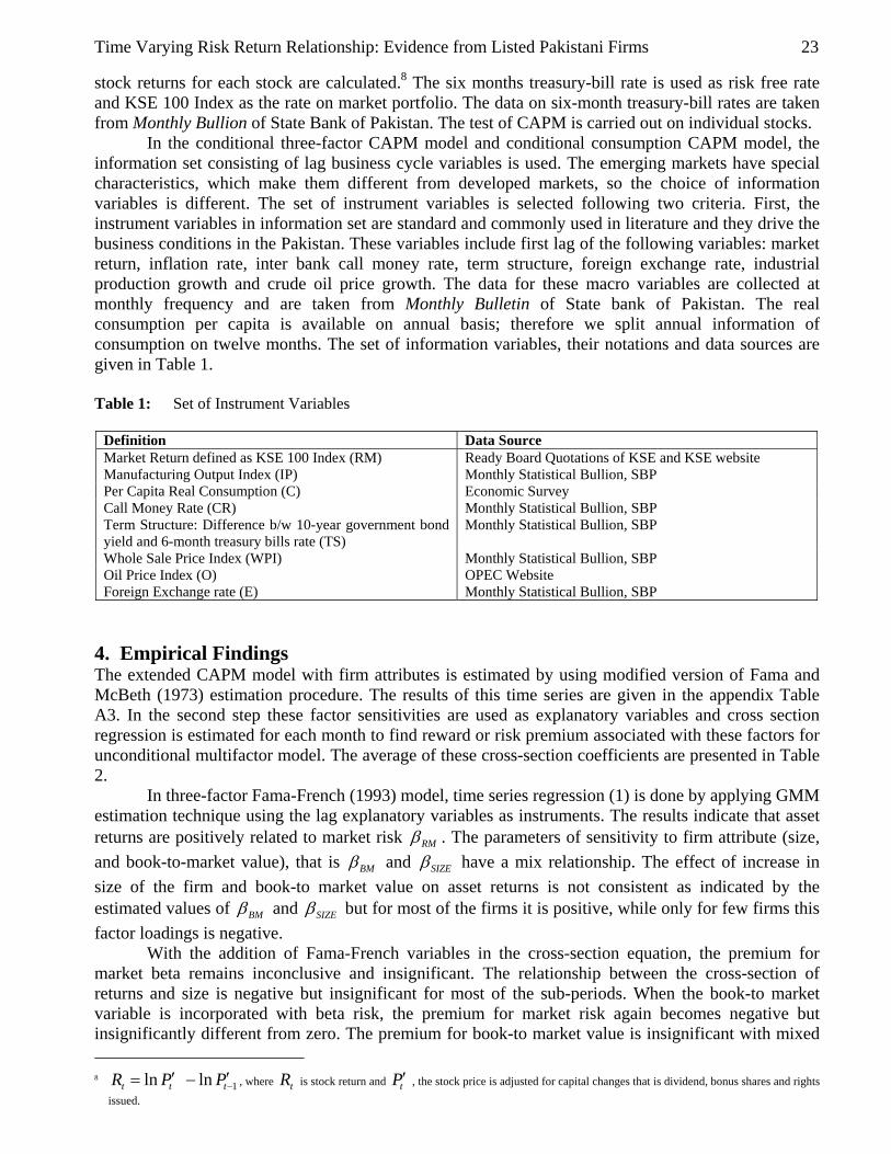
In the conditional three-factor CAPM model and conditional consumption CAPM model, the information set consisting of lag business cycle variables is used. The emerging markets have special characteristics, which make them different from developed markets, so the choice of information variables is different. The set of instrument variables is selected following two criteria. First, the instrument variables in information set are standard and commonly used in literature and they drive the business conditions in the Pakistan. These variables include first lag of the following variables: market return, inflation rate, inter bank call money rate, term structure, foreign exchange rate, industrial production growth and crude oil price growth. The data for these macro variables are collected at monthly frequency and are taken from Monthly Bulletin of State bank of Pakistan. The real consumption per capita is available on annual basis; therefore we split annual information of consumption on twelve months. The set of information variables, their notations and data sources are given in Table 1. Table 1: Set of Instrument Variables

Definition Data Source Market Return defined as KSE 100 Index (RM) Ready Board Quotations of KSE and KSE website Manufacturing Output Index (IP) Monthly Statistical Bullion, SBP Per Capita Real Consumption (C) Economic Survey Call Money Rate (CR) Monthly Statistical Bullion, SBP Term Structure: Difference b/w 10-year government bond yield and 6-month treasury bills rate (TS)

Monthly Statistical Bullion, SBP

Whole Sale Price Index (WPI) Monthly Statistical Bullion, SBP Oil Price Index (O) OPEC Website Foreign Exchange rate (E) Monthly Statistical Bullion, SBP

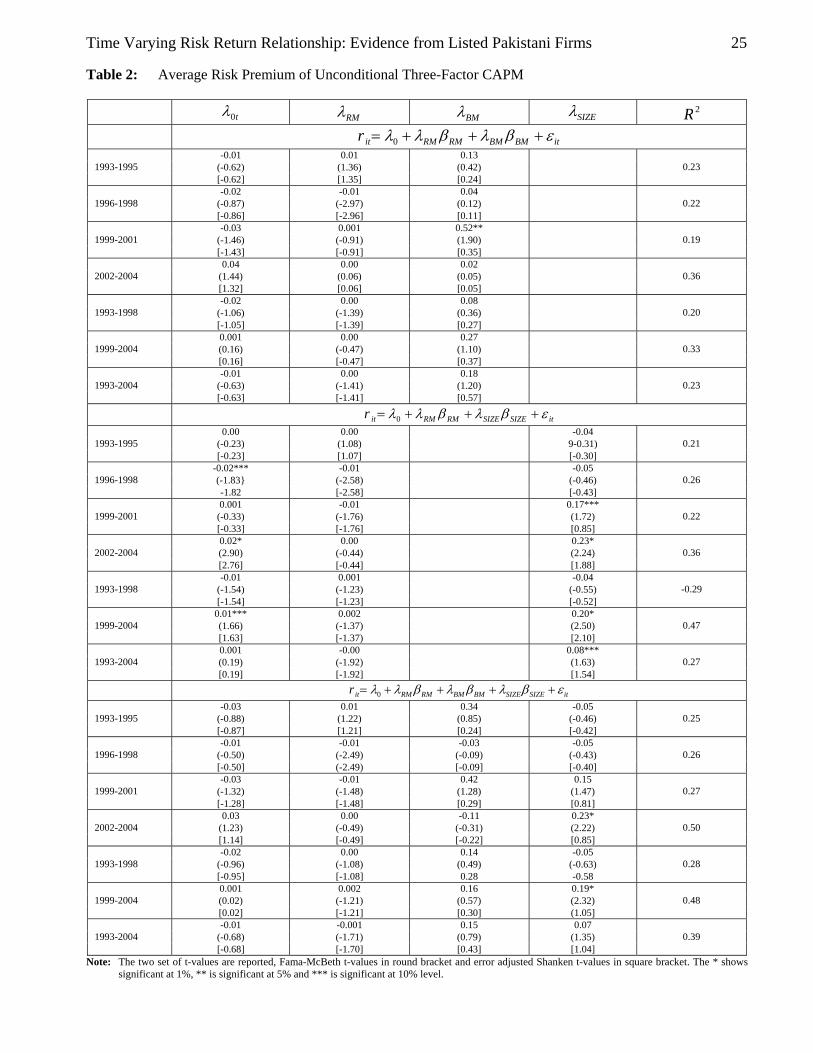
4. Empirical Findings The extended CAPM model with firm attributes is estimated by using modified version of Fama and McBeth (1973) estimation procedure. The results of this time series are given in the appendix Table A3. In the second step these factor sensitivities are used as explanatory variables and cross section regression is estimated for each month to find reward or risk premium associated with these factors for unconditional multifactor model. The average of these cross-section coefficients are presented in Table 2.

In three-factor Fama-French (1993) model, time series regression (1) is done by applying GMM estimation technique using the lag explanatory variables as instruments. The results indicate that asset returns are positively related to market risk RMβ . The parameters of sensitivity to firm attribute (size, and book-to-market value), that is BMβ and SIZEβ have a mix relationship. The effect of increase in size of the firm and book-to market value on asset returns is not consistent as indicated by the estimated values of BMβ and SIZEβ but for most of the firms it is positive, while only for few firms this factor loadings is negative.

With the addition of Fama-French variables in the cross-section equation, the premium for market beta remains inconclusive and insignificant. The relationship between the cross-section of returns and size is negative but insignificant for most of the sub-periods. When the book-to market variable is incorporated with beta risk, the premium for market risk again becomes negative but insignificantly different from zero. The premium for book-to market value is insignificant with mixed 8 1lnln −′−′= ttt PPR , where tR is stock return and tP′ , the stock price is adjusted for capital changes that is dividend, bonus shares and rights

issued.

24 Attiya Y. Javid

sign. The results remain the same when size and book-to-market-value variables are both incorporated in the cross-section model. This suggests that the risk factors associated with market return, size and style of the firm are not significantly rewarded in the market. The intercept terms are significantly different from zero. This result is consistent with findings in literature, such as the one for the UK market by Clare, Priestly and Thomas (1998).


Table 2: Average Risk Premium of Unconditional Three-Factor CAPM

t0λ RMλ BMλ

SIZEλ

2R

itBMBMRMRMitr εβλβλλ +++= 0 -0.01 0.01 0.13

(-0.62) (1.36) (0.42) 1993-1995 [-0.62] [1.35] [0.24]

0.23

-0.02 -0.01 0.04 (-0.87) (-2.97) (0.12) 1996-1998 [-0.86] [-2.96] [0.11]

0.22

-0.03 0.001 0.52** (-1.46) (-0.91) (1.90) 1999-2001 [-1.43] [-0.91] [0.35]

0.19

0.04 0.00 0.02 (1.44) (0.06) (0.05) 2002-2004 [1.32] [0.06] [0.05]

0.36

-0.02 0.00 0.08 (-1.06) (-1.39) (0.36) 1993-1998 [-1.05] [-1.39] [0.27]

0.20

0.001 0.00 0.27 (0.16) (-0.47) (1.10) 1999-2004 [0.16] [-0.47] [0.37]

0.33

-0.01 0.00 0.18 (-0.63) (-1.41) (1.20) 1993-2004 [-0.63] [-1.41] [0.57]

0.23

itSIZESIZERMRMitr εβλβλλ +++= 0

0.00 0.00 -0.04 (-0.23) (1.08) 9-0.31) 1993-1995 [-0.23] [1.07] [-0.30]

0.21

-0.02*** -0.01 -0.05 (-1.83} (-2.58) (-0.46) 1996-1998 -1.82 [-2.58] [-0.43]

0.26

0.001 -0.01 0.17*** (-0.33) (-1.76) (1.72) 1999-2001 [-0.33] [-1.76] [0.85]

0.22

0.02* 0.00 0.23* (2.90) (-0.44) (2.24) 2002-2004 [2.76] [-0.44] [1.88]

0.36

-0.01 0.001 -0.04 (-1.54) (-1.23) (-0.55) 1993-1998 [-1.54] [-1.23] [-0.52]

-0.29

0.01*** 0.002 0.20* (1.66) (-1.37) (2.50) 1999-2004 [1.63] [-1.37) [2.10]

0.47

0.001 -0.00 0.08*** (0.19) (-1.92) (1.63) 1993-2004 [0.19] [-1.92] [1.54]

0.27

itSIZESIZEBMBMRMRMitr εβλβλβλλ ++++= 0

-0.03 0.01 0.34 -0.05 (-0.88) (1.22) (0.85) (-0.46) 1993-1995 [-0.87] [1.21] [0.24] [-0.42]

0.25

-0.01 -0.01 -0.03 -0.05 (-0.50) (-2.49) (-0.09) (-0.43) 1996-1998 [-0.50] (-2.49) [-0.09] [-0.40]

0.26

-0.03 -0.01 0.42 0.15 (-1.32) (-1.48) (1.28) (1.47) 1999-2001 [-1.28] [-1.48] [0.29] [0.81]

0.27

0.03 0.00 -0.11 0.23* (1.23) (-0.49) (-0.31) (2.22) 2002-2004 [1.14] [-0.49] [-0.22] [0.85]

0.50

-0.02 0.00 0.14 -0.05 (-0.96) (-1.08) (0.49) (-0.63) 1993-1998 [-0.95] [-1.08] 0.28 -0.58

0.28

0.001 0.002 0.16 0.19* (0.02) (-1.21) (0.57) (2.32) 1999-2004 [0.02] [-1.21] [0.30] (1.05]

0.48

-0.01 -0.001 0.15 0.07 (-0.68) (-1.71) (0.79) (1.35) 1993-2004 [-0.68] [-1.70] [0.43] [1.04]

0.39

Note: The two set of t-values are reported, Fama-McBeth t-values in round bracket and error adjusted Shanken t-values in square bracket. The * shows significant at 1%, ** is significant at 5% and *** is significant at 10% level.

26 Attiya Y. Javid

Table 3: Average Risk Premium of Conditional Three-Factor CAPM

t0λ RMλ BMλ SIZEλ 2R

itBMcBMrm

cRMtitr εβλβλλ +++= 10

-0.05 0.01 3.88 (-0.89) (0.71) (1.37) 1993-1995 [-0.82] [0.69] [0.03]

0.21

-0.01 0.002 0.39 (-0.50) (-0.12) (0.31) 1996-1998 [-0.49] [-0.11] [0.08]

0.20

0.00 0.00 0.67 (0.04) (0.16) (0.55) 1999-2001 [0.03] [0.16] [0.09]

0.29

t0λ RMλ BMλ SIZEλ 2R

0.05 0.01 0.19 (1.49) (0.28) (0.17) 2002-2004 [1.42] [0.27] [0.08]

0.23

-0.03 0.001 1.98 (-1.03) (0.24) (1.35) 1993-1998 [-1.03] [0.23] [0.07]

0.26

0.03 0.01 0.43 (1.57) (0.58) (0.51) 1999-2004 [1.54] [0.58] [0.12]

0.26

0.00 0.001 1.17 (0.03) (0.58) (1.41) 1993-2004 [0.03] [0.58] [0.12]

0.26

itSIZE

cSIZErm

cRMtitr εβλβλλ +++= 10

0.05 0.01 0.88 (1.38) (0.79) (0.53) 1993-1995 [1.11] [0.77] [0.05[

0.30

-0.13 0.00 4.62*** (-1.86) (-0.20) (1.61) 1996-1998 [-1.42] [-0.19] [0.04]

0.30

0.06 0.01 0.84 (1.14) (0.38) (0.37) 1999-2001 [0.97) [0.37] [0.05]

0.29

0.04 0.01 0.35 (0.84) (0.84) (0.18) 2002-2004 [0.82] [0.83] [0.05]

0.24

-0.05 0.00 2.92*** (-1.10) (0.22) (1.68) 1993-1998 [-1.08) [0.21] [0.66]

0.26

0.05 0.01 0.59 (1.38) (0.44) (0.40) 1999-2004 [1.26) [0.44] [0.07]

0.26


(continued)Table 3: Average Risk Premium of Conditional Three-Factor CAPM

t0λ RMλ BMλ SIZEλ 2R 0.00 0.01 1.34

(0.14) (0.71) (1.17) 1993-2004 [0.14] [0.71] [0.09]

0.26

itSIZE

cSIZEBM

cBMrm

cRMtitr εβλβλβλλ ++++= 10

0.01 0.01 2.67 -1.53 (0.22) (0.78) (0.90) (-0.90) 1993-1995 [0.22] [0.76] [0.03] [-0.05]

0.29

-0.16** 0.00 3.17 4.42 (-1.99) (-0.20) (1.08) (1.52) 1996-1998 [-1.35] [-0.19] [0.04] [0.04]

0.32

0.07 0.00 1.65 0.52 (0.96) (0.22) (0.69) (0.24) 1999-2001 [0.78] [0.22] [0.05] [0.05]

0.30

0.03 0.01 3.40 1.07 (0.48) (0.84) (1.44) (0.56) 2002-2004 [0.48] [0.83] [0.04] [0.05}

0.25

-0.08 0.00 2.94 1.71 (-1.57) (0.21) (1.42) (0.96) 1993-1998 [-1.39] [0.20] [0.05] [0.06]

0.33

0.05 0.01 2.53 0.80 (1.04) (0.67) (1.51) (0.55) 1999-2004 [0.95] [0.67] [0.06] [0.07[

0.28

-0.01 0.00 2.73* 1.24 (-0.31) (0.62) (2.07) (1.09) 1993-2004 [-0.31] [0.61] [0.08] [0.09]

0.35


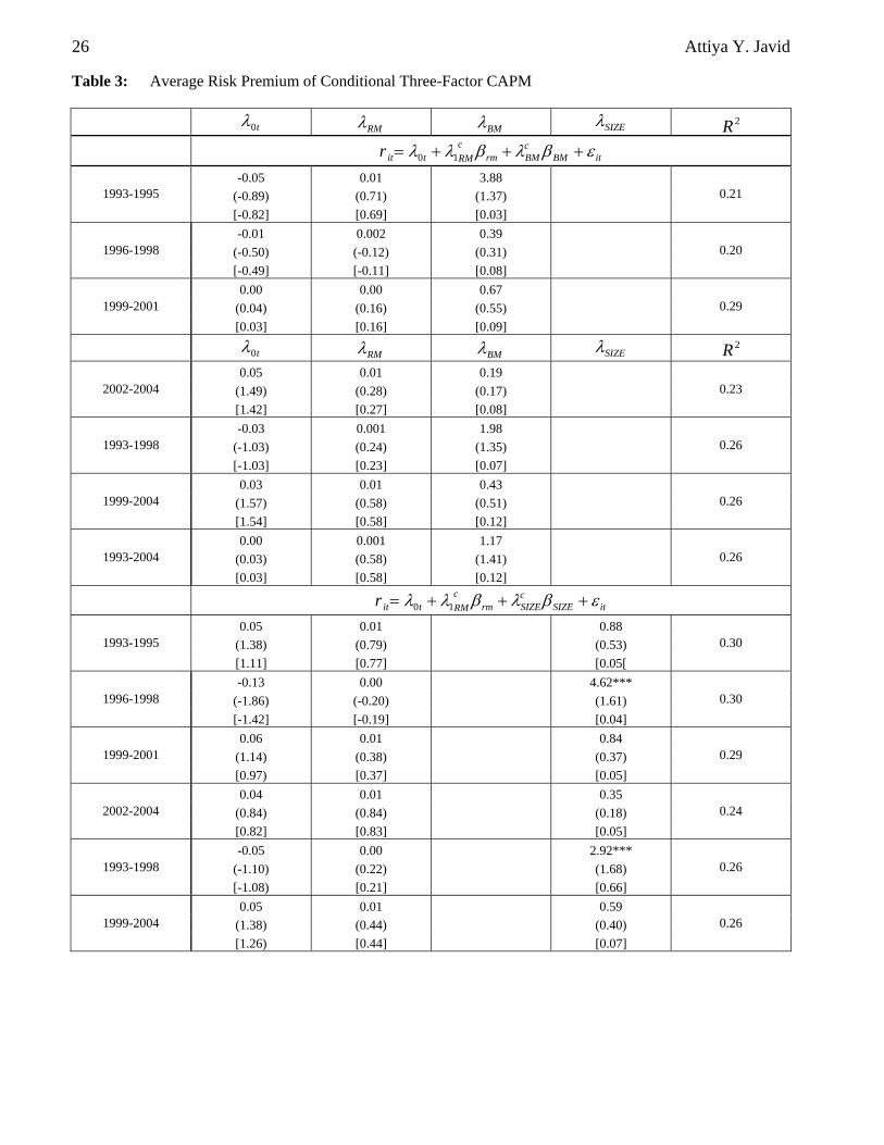
At the next stage of analysis the time variability is allowed in betas and risk premium to

estimate conditional three-factor model. The conditional betas of market return, size and style of firm variables are induced by Dividian-Carroll Method. These variables are conditional on a vector of lagged business-cycle variables. Then these time varying betas are used to estimate time varying risk premium month by month in the second stage. The averages of these risk premiums are reported in Table 3

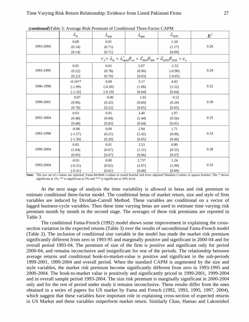
The conditional Fama-French (1992) model shows some improvement in explaining the cross-section variation in the expected returns (Table 3) over the results of unconditional Fama-French model (Table 2). The inclusion of conditional size variable in the model has made the market risk premium significantly different from zero in 1993-95 and marginally positive and significant in 2000-04 and for overall period 1993-04. The premium of size of the firm is positive and significant only for period 2000-04, and remains inconclusive and insignificant for rest of the periods. The relationship between average returns and conditional book-to-market-value is positive and significant in the sub-periods 1999-2001, 1999-2004 and overall period. When the standard CAPM is augmented by the size and style variables, the market risk premium become significantly different from zero in 1993-1995 and 2000-2004. The book-to-market value is positively and significantly priced in 1999-2001, 1999-2004 and in overall sample period 1993-2004. The size risk premium is marginally significant in 2000-2004 only and for the rest of period under study it remains inconclusive. These results differ from the ones obtained in a series of papers for US market by Fama and French (1992, 1993, 1995, 1997, 2004), which suggest that these variables have important role in explaining cross-section of expected returns in US Market and these variables outperform market return. Similarly Chan, Hamao and Lakonishol

28 Attiya Y. Javid

(1991) find a strong relationship between book-to-market value and average return in Japanese market, while Capual, Rowley and Sharpe (1993) observe a similar result that is book-to-market value effect in four European stock markets. Likewise Fama and French (1998) find that the price ratios produce same results for twelve major emerging markets. The findings given in Table 3 also give support to the fact that time varying firm attributes have only limited role in Pakistani market in explaining asset price behavior.

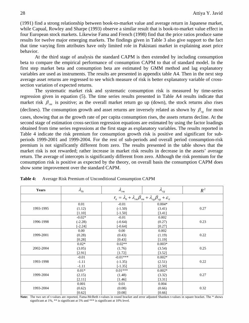
At the third stage of analysis the standard CAPM is then extended by including consumption beta to compare the empirical performance of consumption CAPM to that of standard model. In the first step market beta and consumption beta are estimated by GMM method and lag explanatory variables are used as instruments. The results are presented in appendix table A4. Then in the next step average asset returns are regressed to see which measure of risk is better explanatory variable of cross-section variation of expected returns.

The systematic market risk and systematic consumption risk is measured by time-series regression given in equation (5). The time series results presented in Table A4 results indicate that market risk rmβ is positive; as the overall market return go up (down), the stock returns also rises (declines). The consumption growth and asset returns are inversely related as shown by cgβ for most cases, showing that as the growth rate of per capita consumption rises, the assets returns decline. At the second stage of estimation cross-section regression equations are estimated by using the factor loadings obtained from time series regressions at the first stage as explanatory variables. The results reported in Table 4 indicate the risk premium for consumption growth risk is positive and significant for sub-periods 1999-2001 and 1999-2004. For the rest of sub-periods and overall period consumption-risk premium is not significantly different from zero. The results presented in the table shows that the market risk is not rewarded; rather increase in market risk results in decrease in the assets’ average return. The average of intercepts is significantly different from zero. Although the risk premium for the consumption risk is positive as expected by the theory, on overall basis the consumption CAPM does show some improvement over the standard CAPM. Table 4: Average Risk Premium of Unconditional Consumption CAPM

Years t0λ rmλ cgλ

2R

itcgcgrmrmitr εβλβλλ +++= 0

0.01 -0.01 0.004* (1.12) (-1.50) (3.41) 1993-1995 [1.10] [-1.50] [3.41]

0.27

-0.02* -0.01 0.002 (-2.28) (-0.64) (0.27) 1996-1998 [-2.24] [-0.64] [0.27]

0.23

0.00 0.00 0.002 (0.28) (0.43) (1.19) 1999-2001 [0.28] [0.43] [1.19]

0.22

0.02* 0.02** 0.003* (3.05) (1.76) (3.54) 2002-2004 [2.91] [1.72] [3.52]

0.25

-0.01 -0.01*** 0.002* -1.11 (-1.35) (2.51) 1993-1998 -1.11 [-1.35] [2.50]

0.22

0.01* 0.01*** 0.002* (2.15) (1.48) (3.32) 1999-2004 [2.11] [1.46] [3.31]

0.27

0.001 0.01 0.004 (0.62) (0.08) (0.66) 1993-2004 [0.62] [0.08] [0.66]

0.32



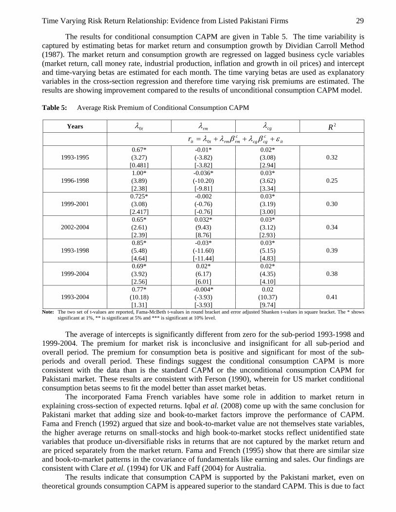
The results for conditional consumption CAPM are given in Table 5. The time variability is captured by estimating betas for market return and consumption growth by Dividian Carroll Method (1987). The market return and consumption growth are regressed on lagged business cycle variables (market return, call money rate, industrial production, inflation and growth in oil prices) and intercept and time-varying betas are estimated for each month. The time varying betas are used as explanatory variables in the cross-section regression and therefore time varying risk premiums are estimated. The results are showing improvement compared to the results of unconditional consumption CAPM model. Table 5: Average Risk Premium of Conditional Consumption CAPM

Years t0λ rmλ cgλ

2R it

ccgcg

crmrmtitr εβλβλλ +++= 0

0.67* -0.01* 0.02* (3.27) (-3.82) (3.08) 1993-1995 [0.481] [-3.82] [2.94]

0.32

1.00* -0.036* 0.03* (3.89) (-10.20) (3.62) 1996-1998 [2.38] [-9.81] [3.34]

0.25

0.725* -0.002 0.03* (3.08) (-0.76) (3.19) 1999-2001 [2.417] [-0.76] [3.00]

0.30

0.65* 0.032* 0.03* (2.61) (9.43) (3.12) 2002-2004 [2.39] [8.76] [2.93}

0.34

0.85* -0.03* 0.03* (5.48) (-11.60) (5.15) 1993-1998 [4.64] [-11.44] [4.83]

0.39

0.69* 0.02* 0.02* (3.92) (6.17) (4.35) 1999-2004 [2.56] [6.01] [4.10]

0.38

0.77* -0.004* 0.02 (10.18) (-3.93) (10.37) 1993-2004 [1.31] [-3.93] [9.74]

0.41


The average of intercepts is significantly different from zero for the sub-period 1993-1998 and

1999-2004. The premium for market risk is inconclusive and insignificant for all sub-period and overall period. The premium for consumption beta is positive and significant for most of the sub-periods and overall period. These findings suggest the conditional consumption CAPM is more consistent with the data than is the standard CAPM or the unconditional consumption CAPM for Pakistani market. These results are consistent with Ferson (1990), wherein for US market conditional consumption betas seems to fit the model better than asset market betas.

The incorporated Fama French variables have some role in addition to market return in explaining cross-section of expected returns. Iqbal et al. (2008) come up with the same conclusion for Pakistani market that adding size and book-to-market factors improve the performance of CAPM. Fama and French (1992) argued that size and book-to-market value are not themselves state variables, the higher average returns on small-stocks and high book-to-market stocks reflect unidentified state variables that produce un-diversifiable risks in returns that are not captured by the market return and are priced separately from the market return. Fama and French (1995) show that there are similar size and book-to-market patterns in the covariance of fundamentals like earning and sales. Our findings are consistent with Clare et al. (1994) for UK and Faff (2004) for Australia.

The results indicate that consumption CAPM is supported by the Pakistani market, even on theoretical grounds consumption CAPM is appeared superior to the standard CAPM. This is due to fact

30 Attiya Y. Javid

that consumption beta contain much more information than the market beta. These findings are contrast to US findings by Mankiw and Shapiro (1988) and Germany by Sauer and Murphy (1992). 5. Conclusions The standard CAPM is extended with Fama-French (1992) variables, size and book-to-market value, in unconditional and conditional setting. The observation is that the dynamic size and style coefficient explain the cross-section of expected returns in some sub-periods. The consumption risk is incorporated in standard CAPM in static and dynamic way. The findings reveal that the market rewards systematic risk for higher returns, but the relevant measure for systematic risk appears to be conditional consumption beta rather than market beta. This evidence leads to investigate macroeconomic risks that can describe the variation in expected return in a more complete and meaningful way. Acknowledgement The study is based on Ph D dissertation of Attiya Y. Javid. The author wishes to thank Dr Eatzaz Ahmad, Dr Rashid Amjad, Dr Abdul Qayyum, Dr Fazal Hussain and Tariq Mahmood for their valuable comments. She is grateful to Muhammad Ali Bhatti for providing assistance in compiling data. The usual disclaimer applies. References [1] Ahmad Eatzaz and Badar-u-Zaman (1999) Volatility and Stock Return at Karachi Stock

Exchange. Pakistan Economic and Social Review 37:1, 25–37. [2] Ahmad Eatzaz and Mohammad Ali Qasim (2004) Stock Market Volatility in Pakistan: An

Empirical Analysis. The Middle East Business and Economic Review 16:2. [3] Bark, Hee-Kyung K. (1991) Risk, Return and Equilibrium in the Emerging markets: Evidence

from the Korean stock market. Journal of Economics and Business 43, 353–362. [4] Banz, Rolf (1981) The Relationship between Returns and Market Value of Common Stocks.

Journal of Financial Economics 9:1, 3–18. [5] Backus, David K., Allan W. Gregory and Stanley E. Zin (1989) Risk Premium in the Term

Structure: Evidence from Artificial Economics. Journal of Monetary Economics 24, 371–399. [6] Basu, S. (1977) Investment Performance of Common Stocks in Relation to their Price Earnings

Ratios: A Test of Efficient Market Hypothesis. Journal of Finance, 12:3, 129–56. [7] Banz, Rolf (1981) The Relationship between Returns and Market Value of Common Stocks.

Journal of Financial Economics 9:1, 3–18. [8] Bhandari, Laxmi Chand (1988) Debt/Equity Ratio and Expected Common Stock Returns:

Empirical evidence. Journal of Finance 43:2, 507–528. [9] Breeden, Douglas (1978) An Intertemporal Asset Pricing Model with Stochastic Consumption

and Investment Opportunities. Journal of Financial Economics 7, 265–296. [10] Breeden, Douglas, Michael R. Gibbons and Robert H. Litzenberger (1989) Empirical Tests of

the Consumption-oriented CAPM. Journal of Finance 44, 231–262. [11] Chan, Lious K. C., Yasushi Hamoa, and Josef Lakonishok (1991) Fundamentals and Stock

Return in Japan. Journal of Finance 46:5, 1739–1789. [12] Chung, Y. P., Johnson H., and M. J. Schill (2001) Asset Pricing when Returns are Non-normal:

Fama- French Variables Versus Higher-Order Systematic Co-movement. A. Gary Anderson Graduate School of Management. University of California, Riverside. (Working Paper)

[13] Clare, A. D., R. Priestley, and S. H. Thomas (1998) Report of Beta’s Death are Premature: Evidence from the UK. Journal of Banking and Finance 22, 1207–1229.

[14] Capual Carlo, Ian Rowley and William F. Sharpe (1993) International Value and Growth Stock Returns. Financial Analysis Journal, January/February, 27–36.


[15] Cochrane, John H. (2001) Asset Pricing. New Jersey: Princeton University Press. [16] Cochrane, John H. (1996) A Cross-Sectional Test of an Investment Based Asset Pricing Model.

Journal of Political Economy 104, 572–621. [17] Campbell, John Y. (2000) Asset Pricing at the Millennium. Journal of Finance 60, 1515–1567. [18] Campbell, John Y. and John H. Cochrane (1999) By Force of Habit: A Consumption Based

Explanation of Aggregate Stock Market Behavior. Journal of Political Economy 107, 205–251. [19] Chen, Nai-Fa., R. R. Roll, and S. A. Ross (1986) Economic Forces and Stock Market. Journal

of Business 59, 383–403. [20] Cox, John C., Jonathan E. Ingersoll, and Stephen A. Ross (1985) A Theory of the Term

Structure of Interest Rates. Econometrica 53, 385–408. [21] Davidian, Marie and Raymond J. Carroll (1987) Variance Function Estimation. Journal of the

American Statistical Association, 1079–1091. [22] Elton, Edward. J., Martin, J. Gruber, and Christopher R. Blake (1995) Fundamental Economic

Variables, Expected Return and Bond Fund Performance. Journal of Finance 50, 1229–1256. [23] Faff, Robert (2001) A Multivariate Test of a Dual-Beta CAPM: Australian Evidence. The

Financial Review, 36, 157-174. [24] Fama, Eugene F. (1965) The Behavior of Stock Market Prices. Journal of Business, 38, 34–10. [25] Fama, Eugene F. and Kenneth R. French (1989) Business Conditions and Expected Returns.

Journal of Financial Economics 25, 23–50. [26] Fama, Eugene F. and Kenneth R. French (1992) The Cross Section of Expected Return. Journal

of Finance 47:2, 427–465. [27] Fama, Eugene F. and Kenneth R. French (1993) Common Risk Factors in the Returns of Stocks

and Bonds. Journal of Financial Economics 33, 3–56. [28] Fama, Eugene F. and Kenneth R. French (1996) Multifactor Explanation of Asset Pricing

Anomalies. Journal of Finance, 51, 55–87. [29] Fama, Eugene F. and Kenneth R. French (2004) The Capital Asset Pricing Model: Theory and

Evidence. Journal of Economic Perspectives 18:1, 25–46. [30] Fama, Eugene F. and James D. MacBeth (1973) Risk, Return and Equilibrium: Empirical Tests.

Journal of Political Economy, 81(3), 607–36. [31] Ferson, W. E. (1991) Are the Latent Variables in Time Varying Expected Returns

Compensation for Consumption Risk? Journal of Finance 45, 397–430. [32] Ferson, Wayne E. and Campbell R. Harvey (1991) The Variation of Economic Risk Premiums.

Journal of Political Economy, 99, 385–415. [33] Ferson, Wayne E. and Campbell R. Harvey (1993) The Risk and Predictability of International

Equity Returns. Review of Financial Studies, 6, 527–566. [34] Ferson Wayne E. and Campbell R. Harvey (1999) Economic, Financial and Fundamental

Global Risk In and Out of EMU. Swedish Economic Policy Review, 6, 123–184. [35] Ferson, W. and C. Korajczyk (1995) Do Arbitrage Model Explain the Predictability of Stock

Returns? Journal of Business 68, 309–349. [36] Ferson Wayne E., S. Kandel and R. Stambaugh (1986) Tests of Asset Pricing with Time-

varying expected risk Premium and Market Betas. Journal of Finance 42, 201–220. [37] Gibbons, M. R. and W. E. Ferson (1985) Tests of Asset Pricing Models with Changing

Expectations and an Unobservable Market Portfolio. Journal of Financial Economics 14, 217–236

[38] Grossman, Sanford (1981) Further Results on the Informational Efficiency of Stock Markets. Stanford University, Stanford. (Mimeographed)

[39] Harvey, C. R. (1989) Time-Varying Conditional Covariance in Tests of Asset Pricing Models. Journal of Financial Economics 24, 289–318.

[40] Harvey, C. R. and A. Siddique (1999) Autoregressive Conditional Skewness. Journal of Financial and Quantitative Analysis 34, 456–487.

32 Attiya Y. Javid

[41] Harvey, C. R. (1995) Predictable Risk and Return in Emerging Markets. The Review of Financial Studies 8, 773–816.

[42] Hsieh, D. A. and M. H. Miller (1990) Margin Regulations and the Stock Market Volatility. Journal of Finance 45, 3–30.

[43] Hazuka, T. (1984) Consumption Beta and Backwardation in the Commodity Market. Journal of Finance 39, 647–655.

[44] Hansen, Lars P., (1982) Large Sample Properties of Generalized Method of Moments Estimators. Econometrica 50, 1029–1054.

[45] Hansen, Lars P. and Kenneth Singleton (1982) Generalized Instrument Variables Estimation in Non-linear Rational Expectation Model. Econometrica 50, 1269–1286.

[46] Hansen, Lars P. and Kenneth Singleton (1983) Stochastic Consumption, Risk Aversion and the Temporal Behavior of Asset Return. Journal of Political Economy 91, 249–265.

[47] Iqbal, Javed and R. D. Brooks (2007) Alternate Beta Risk Estimation and Asset Pricing Test in Emerging Market: Case of Pakistan. Multinational Journal of Finance 17, 75-93.

[48] Iqbal, Javed, Robert Brooks and D. U. Galagedera (2008) Testing Conditional Asset Pricing Model: An Emerging Market Perspective. Working Paper 3/08. Monash University, Australia.

[49] Javid, Attiya Y. and Eatzaz Ahmad (2008) The Conditional Capital Asset Pricing Model: Evidence from Pakistani Listed Companies. PIDE Working Paper 48.

[50] Javid, Attiya Y. and Eatzaz Ahmad (2008) Testing The Multi-Moment Asset Pricing Behavior of the Listed firms at Karachi Stock Exchange. PIDE Working Paper 49.

[51] Jagannathan, R. and Z. Wang (1996) The Conditional CAPM and the Cross Section of Expected Return. Journal of Finance 51, 3–53.

[52] Kandel, Shmuel and Robert F. Stambaugh (1989) A Mean variance Framework for Tests of Asset Pricing Models. Review of Financial Studies 2, 125–156.

[53] Kandel, Shmuel and Robert F. Stambaugh (1995) Portfolio Inefficiency and the Cross-section of Expected Return. Journal of Finance 50, 157–184.

[54] Kothari, S. P., Jay Shanken and Richard G. Sloan (1995) Another Look at the Cross Section of Expected Stock Returns. Journal of Finance 50:1, 185–224.

[55] Lintner, J. (1965) The Valuation of Risk Assets and Selection of Risky Investments in Stock Portfolio and Capital Budgets. Review of Economics and Statistics 47:1, 13–47.

[56] Lakonishok, Josef, Andrie Shliefer and W. Vishney Robeert (1994) Contrarian Investment Extrapolation and Risk. Journal of Finance 49, 1541–1578.

[57] Lucas, Robert E. Jr. (1978) Asset Prices in an Exchange Economy. Econometrica 46, 1429–1445.

[58] Merton, Robert C. (1973) An Intertemporal Capital Asset Pricing Model. Econometrica 41:5, 867–87.

[59] Mehra, Rajnash and Edward C. Prescott (1985) The Equity Premium: The Puzzle. Journal of Monetary Economics 15, 145–161.

[60] Mankiw N. Gregory and Mathew D. Shapiro (1988) Risk and Return: Consumption Beta versus Market Beta. The Review of Economics and Statistics 48, 452–459.

[61] Pakistan, Government of (Various Issues) Pakistan Economic Survey [62] Ross, S. A., (1976) The Arbitrage Pricing Theory of Capital Asset Pricing, Journal of

Economic Theory 13(3), 341-60. [63] Roll, Richard W. and Stephen A. Ross (1980) An empirical Investigation of Arbitrage Pricing

Theory. Journal of Finance, 35, 1073-1103. [64] Reinganum, Marc R., (1981) Misspecification of Capital Asset Pricing: Empirical Anomalies

Based on Earnings Yields and Market Values. Journal of Financial Economics 9, 19-46. [65] Rosenberg, Barr, Kenneth Reid and Ronald Lanstein (1985) Persuasive Evidence of the Market

Inefficiency, Journal of Portfolio Management, 11 9-17. [66] Scholes, M. and J. Williams (1977) Estimating Beta from Nonsynchronous Data, Journal of

Financial Economics 5, 309-327.


[67] Schwert, William G. (1989) Why Does the Stock Price Volatility Change Over Time? Journal of Finance, 44. 1115-1153.

[68] Schwert William G. and P. Seguin (1990) Heteroscedasticity in Stock Returns. Journal of Finance. 45. 1129-1155

[69] Shanken, Jay, (1992) On the Estimation of Beta Pricing Models. Review of Financial Studies 5, 1-34.

[70] Sauer, A. and A. Murphy (1992) An Empirical Comparison of Alternative Models of Capital Asset Pricing in Germany. Journal of Banking and Finance, 16.

[71] Sharpe, W. F., (1964) Capital Asset Prices: A Theory of Market Equilibrium under Conditions of Risk. Journal of Finance 19(3), 425-442.

[72] State Bank of Pakistan, Monthly Statistical Bulletin, (various issues. Karachi). [73] Tinic, Seha M. and Richard R. West (1984). Risk and Return: January versus the Rest of the

Year. Journal of Financial Economics. 13(4), 561-574. [74] Wheatley, Simon (1988a) Some Tests of Consumption Based Asset Pricing Model, Journal of

Monetary Economics, 22, 639-655 [75] Wheatley, Simon (1988b) Some Tests of Consumption Based Asset Pricing Model Journal of

Financial Economics, 21, 171-212 [76] Weil, Philippe (1989) The Equity Premium Puzzle and the Risk Free Rate Puzzle. Journal of

Monetary Economics, 24, 401-421

34 Attiya Y. Javid

Appendix A Table A1: List of Companies included in the Sample

Name of Company Symbol Sector Al-Abbas Sugar AABS Sugar and Allied Askari Commercial Bank ACBL Insurance and Finance Al-Ghazi Tractors AGTL Auto and Allied Adamjee insurance Company AICL Insurance Ansari Sugar ANSS Sugar and Allied Askari Leasing ASKL Leasing Company Bal Wheels BWHL Auto and Allied Cherat Cement CHCC Cement Crescent Textile Mills CRTM Textile Composite Crescent Steel CSAP Engineering Comm. Union Life Assurance CULA Insurance and Finance Dadabhoy Cement DBYC Cement Dhan Fibres DHAN Synthetic and Rayon Dewan Salman Fibre DSFL Synthetic and Rayon Dewan Textile DWTM Textile Composite Engro Chemical Pakistan ENGRO Chemicals and Pharmaceuticals Faisal Spinning. FASM Textile Spinning FFCL Jordan FFCJ Chemicals and Pharmaceuticals Fauji Fertilizer FFCL Fertilizer Fateh Textile FTHM Textile Composite General Tyre and Rubber Co. GTYR Auto and Allied Gul Ahmed Textile GULT Textile Composite Habib Arkady Sugar HAAL Sugar and Allied Hub Power Co. HUBC Power Generation & Distribution I.C.I. Pak ICI Chemicals and Pharmaceuticals Indus Motors INDU Auto and Allied J.D.W. Sugar JDWS Sugar and Allied Japan Power JPPO Power Generation & Distribution Karachi Electric Supply Co. KESC Power Generation & Distribution Lever Brothers Pakistan LEVER Food and Allied Lucky Cement LUCK Cement Muslim Commercial Bank MCB Commercial Banks Maple Leaf Cement MPLC Cement National Refinery NATR Fuel and Energy Nestle Milk Pak Ltd NESTLE Food and Allied Packages Ltd. PACK Paper and Board Pak Electron PAEL Cables and Electric Goods Pakistan Tobacco Company PAKT Tobacco Pakland Cement PKCL Cement Pakistan State Oil Company. PSOC Fuel and Energy PTCL (A) PTC Fuel and Energy Southern Electric SELP Cables and Electric Goods ICP SEMF Modarba SEMF Modarba Sitara Chemical SITC Chemicals and Pharmaceuticals Sui Southern Gas Company SNGC Fuel and Energy Sui Northern Gas Company SSGC Fuel and Energy Tri-Star Polyester Ltd TSPI Synthetic and Rayon Tri-Star Shipping Lines TSSL Transport and Communication Unicap Modarba UNIM Modarba


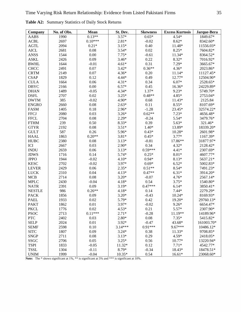
Table A2: Summary Statistics of Daily Stock Returns

Company No. of Obs. Mean St. Dev. Skewness Excess Kurtosis Jarque-Bera AABS 1990 0.13** 3.57* 0.65* 4.54* 1849.67* ACBL 2697 0.10*** 2.81* -0.02 8.62* 8342.60* AGTL 2094 0.21* 3.15* 0.40 11.48* 11556.03* AICL 2681 0.08 3.54* 0.02 8.25* 7604.82* ANSS 1544 0.00 7.75* -0.61 11.34* 8364.52* ASKL 2426 0.09 3.46* 0.22 8.32* 7016.92* BWHL 1644 -0.01 4.61* 0.31 7.29* 3665.67* CHCC 2491 0.07 3.42* 0.36** 4.36* 2023.86* CRTM 2149 0.07 4.36* 0.20 11.14* 11127.45* CSAP 1829 0.12 4.44* 0.49 12.77* 12504.90* CULA 1664 0.06 4.31* 0.34 6.07* 2528.65* DBYC 2166 0.00 6.57* 0.45 16.36* 24229.89* DHAN 1489 -0.05 4.34* 1.37* 9.23* 5749.70* DSFL 2707 0.02 3.25* 0.48** 4.85* 2753.04* DWTM 385 -0.02 4.90* 0.68 11.43* 2125.84 ENGRO 2660 0.08 2.63* 0.11 8.55* 8107.69* FASM 1405 0.18 2.96* -1.28 23.45* 32574.22* FFCJ 2080 0.03 3.26* 0.62** 7.23* 4656.48* FFCL 2704 0.08 2.29* -0.24 5.54* 3479.76* FTHM 239 0.50 8.33* 0.39 5.63* 321.46* GTYR 2192 0.08 3.51* 1.40* 13.89* 18339.20* GULT 587 0.26 5.96* 0.43* 10.28* 2601.98* HAAL 1863 0.20** 3.81* 0.45* 3.77* 1167.39* HUBC 2380 0.08 3.13* -0.81 17.86** 31877.97* ICI 2667 0.03 2.90* 0.34 4.32* 2128.42* INDU 2659 0.06 3.13* 0.59*** 4.41* 2307.69* JDWS 1716 0.14 5.74* 0.25* 8.01* 4607.77* JPPO 1944 -0.02 4.10* 0.94* 8.13* 5637.21* KESC 2702 -0.02 3.97* 0.69* 6.52* 5002.83* LEVER 2429 0.06 2.35* 0.51** 8.54* 7491.23* LUCK 2310 0.04 4.13* 0.47** 6.31* 3914.20* MCB 2714 0.08 3.20* -0.07 4.76* 2567.14* MPLC 2430 -0.04 4.18* 0.54 3.75* 1540.80* NATR 2391 0.09 3.19* 0.47*** 6.14* 3850.41* NESTLE 986 0.26** 4.18* 0.14 7.44* 2279.29* PACK 1856 0.09 3.20* -0.43 10.24* 8169.93* PAEL 1933 0.02 5.79* 0.42 19.20* 29760.13* PAKT 1862 0.01 3.97* -0.02 9.26* 6654.47* PKCL 1776 0.02 4.53* 0.21 5.57* 2307.90* PSOC 2713 0.11*** 2.71* -0.28 11.19** 14189.96* PTC 2402 0.03 2.80* 0.08 7.35* 5415.82* SELP 2024 0.01 3.92* -0.47 43.68* 161003.70* SEMF 2598 0.10 3.14*** 0.91*** 9.67*** 10486.12* SITC 1807 0.09 3.24* 0.38 11.33* 9708.85* SNGP 2711 0.08 3.13* 0.29 4.59* 2418.05* SSGC 2706 0.05 3.25* 0.56 10.77* 13220.94* TSPI 1833 -0.05 11.32* 0.12 7.71* 4542.77* TSSL 1304 -0.11 8.79* -0.34 18.43* 18478.51* UNIM 1999 -0.04 10.35* 0.54 16.61* 23068.60*

Note: The * shows significant at 1%, ** is significant at 5% and *** is significant at 10%.

36 Attiya Y. Javid

Table A3 : The Coefficients of Three Factor Sensitivities

t0β rmβ BMβ SIZEβ

2R AABS -0.02 0.30* -0.03* 0.06*** 0.19 ACBL 0.03 0.95* 0.01 0.00 0.53 AGTL 0.14*** 0.38* 0.04* 0.04* 0.18 AICL 0.17 1.46* 0.002 -0.02 0.51 ANSS 0.47* 0.46 0.06* 0.002* 0.23 ASKL -0.27*** 0.87* 0.01 0.06* 0.41 BWHL -0.44* 0.16 -0.01 0.06* 0.47 CHCC 0.32* 0.90* 0.04* 0.01** 0.54 CRTM 0.31*** 0.91* 0.02* -0.01 0.40 CSAP 0.10 0.63* 0.02* 0.01 0.26 CULA 0.10 0.40* 0.00 -0.01 0.21 DBYC 0.33*** 1.15* 0.04* 0.01 0.41 DHAN -0.04 1.10* 0.02 0.03 0.46 DSFL 0.01 1.33* 0.003 0.002 0.56 DWTM 0.40 0.34* 0.04* 0.02 0.33 ENGRO 0.08 0.76* 0.002 -0.01 0.35 FASM 0.20 0.58* 0.04* 0.04 0.24 FFCJ -0.31 -0.07 0.00 0.03 0.42 FFCL 0.10 0.81* 0.00 -0.01 0.52 FTHM -0.01 0.05 0.00 0.00 0.41 GTYR 0.57 0.73* 0.04* -0.02 0.31 GULT -0.31 0.13 0.00 0.04 0.44 HAAL 0.03 0.52 0.03 0.04 0.23 HUBC -0.57 1.33 0.00 0.06 0.72 ICI 0.04 1.26 0.00 -0.01 0.61 ICPSEMF 0.38 0.98 0.01 -0.03 0.49 INDU 0.44 0.77 0.04 0.00 0.47 JDWS 0.26 0.42 0.04 0.01 0.35 JPPO 0.15 0.82 0.01 -0.01 0.40 KESC -0.31* 1.58* 0.01 0.05* 0.68 LEVER 0.09 1.07* 0.01 0.00 0.49 LUCK -0.11 0.50* 0.01* 0.03 0.32 MCB 0.15 1.18* 0.00 -0.01 0.64 MPLC 0.09 1.18* 0.01 0.01 0.45 NATR 0.26** 0.75* 0.02* 0.00 0.39 NESTLE -0.03 0.01 0.00 0.01 0.41 PACK 0.04 0.65* 0.01 0.01 0.36 PAEL 0.09 0.64** 0.03** 0.03** 0.39 PAKT -0.15 0.53** 0.01 0.03** 0.47 PKCL 0.00 0.62* 0.01 0.02 0.42 PSO 0.29* 1.30* 0.00 -0.03 0.73 PTC 0.26 1.09* -0.01 -0.03 0.74 SELP 0.08 0.86* 0.01 -0.01 0.32 SITC 0.13 0.50* 0.01 0.00 0.48 SNGP 0.07 1.30* 0.00 0.00 0.71 SSGC 0.13 1.22* 0.00 -0.02 0.72 TSPI 0.33 0.70* 0.06 0.02 0.43 TSSl 0.09 0.70* 0.03 0.03 0.33 UNIM 0.17 0.70* 0.05* 0.03 0.51



Table A4: The Coefficient of asset Sensitivity to Market Factor and Consumption

t0β rmβ cgβ

2R

AABS -0.40 -0.80 10.87* 0.42 ACBL 0.34 1.74* -8.54 0.21 AGTL 0.04 0.90* -0.43 0.03 AICL 0.16 1.25* -3.84 0.49 ANSS -0.29 0.34 7.54 0.38 ASKL -0.07 0.81* 2.04 0.38 BWHL -0.40 -0.11 10.60 0.48 CHCC -0.33 0.31 8.89** 0.21 CRTM -0.08 1.05 2.68 0.37 CSAP -0.34 0.14 9.32*** 0.43 CULA -0.54 -0.72 14.50* 0.40 DBYC 0.18 1.38* -5.08 0.36 DHAN 0.12 1.54* -3.53 0.36 DSFL 0.54 1.84* -14.36* 0.48 DWTM 0.26 -0.29 -6.69 0.35 ENGRO -0.04 0.13 1.20 0.51 FASM 0.13 1.63* -2.95 0.37 FFCJ -0.03 0.06 0.90 0.36 FFCL -0.04 0.92* 1.58 0.51 FTHM -0.11 0.04 3.04 0.39 GTYR -0.29 0.70* 8.38* 0.40 GULT 0.15 0.77 -3.78 0.31 HAAL -0.12 0.31 3.59 0.42 HUBC 0.04 0.96* -0.62 0.61 ICI -0.03 1.01* 0.74 0.58 ICPSEMF -0.27 -0.22 7.37 0.26 INDU -0.20 0.80* 5.28 0.36 JDWS -0.38 0.72** 10.74 0.51 JPPO -0.01 0.70 0.16 0.36 KESC 0.07 0.98* -2.07 0.57 LEVER -0.30 0.51 8.57 0.31 LUCK -0.12 0.47 3.38 0.30 MCB 0.22 1.49 -5.53 0.60 MPLC -0.06 1.58 1.87 0.40 NATR -0.35 0.47 9.53 0.23 NESTLE -0.06 0.31 1.95 0.40 PACK -0.12 0.74 3.67 0.35 PAEL 0.05 1.16 -1.21 0.42 PAKT -0.11 -0.24 2.81 0.34 PKCL 0.03 0.41 -0.60 0.40 PSO 0.19 1.54 -4.63 0.69 PTC 0.19 1.87 -4.64 0.34 SELP -0.27 -0.46 7.28 0.50 SITC -0.22 -0.25 6.14 0.32 SNGP 0.22 1.82 -5.50 0.57 SSGC 0.15 1.04 -3.73 0.72 TSPI -0.04 1.22 0.33 0.34 TSSl 0.28 1.08 -8.61 0.52 UNIM 0.35 2.53 -9.27 0.46


38 Attiya Y. Javid

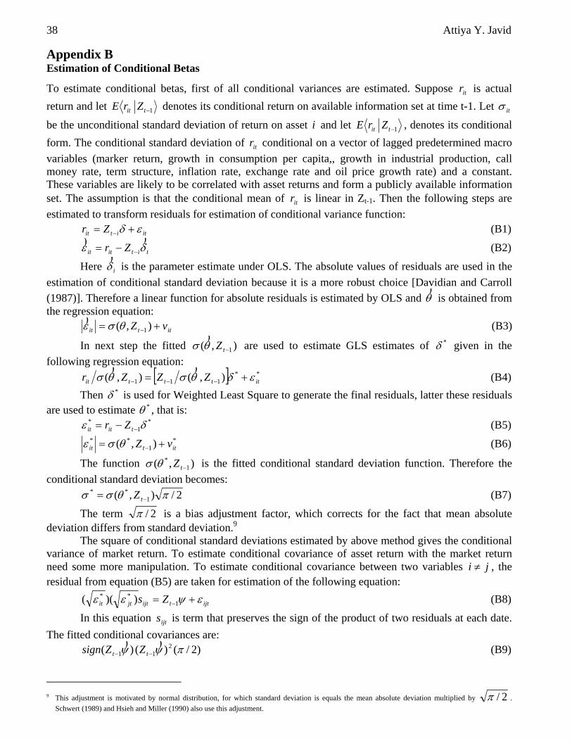
Appendix B Estimation of Conditional Betas

To estimate conditional betas, first of all conditional variances are estimated. Suppose itr is actual return and let 1−tit ZrE denotes its conditional return on available information set at time t-1. Let itσ

be the unconditional standard deviation of return on asset i and let 1−tit ZrE , denotes its conditional form. The conditional standard deviation of itr conditional on a vector of lagged predetermined macro variables (marker return, growth in consumption per capita,, growth in industrial production, call money rate, term structure, inflation rate, exchange rate and oil price growth rate) and a constant. These variables are likely to be correlated with asset returns and form a publicly available information set. The assumption is that the conditional mean of itr is linear in Zt-1. Then the following steps are estimated to transform residuals for estimation of conditional variance function:

ititit Zr εδ += − (B1)

tititit Zr δε))

−−= (B2)

Here iδ)

is the parameter estimate under OLS. The absolute values of residuals are used in the estimation of conditional standard deviation because it is a more robust choice [Davidian and Carroll (1987)]. Therefore a linear function for absolute residuals is estimated by OLS and θ

) is obtained from

the regression equation: ittit vZ += − ),( 1θσε) (B3)

In next step the fitted ),( 1−tZθσ)

are used to estimate GLS estimates of *δ given in the following regression equation:

[ ] **111 ),(),( ittttit ZZZr εδθσθσ += −−−

)) (B4)

Then *δ is used for Weighted Least Square to generate the final residuals, latter these residuals are used to estimate *θ , that is:

*1

* δε −−= titit Zr (B5) *

1** ),( ittit vZ += −θσε (B6)

The function ),( 1*

−tZθσ is the fitted conditional standard deviation function. Therefore the conditional standard deviation becomes:

2/),( 1** πθσσ −= tZ (B7)

The term 2/π is a bias adjustment factor, which corrects for the fact that mean absolute deviation differs from standard deviation.9

The square of conditional standard deviations estimated by above method gives the conditional variance of market return. To estimate conditional covariance of asset return with the market return need some more manipulation. To estimate conditional covariance between two variables ji ≠ , the residual from equation (B5) are taken for estimation of the following equation:

ijttijtjtit Zs εψεε += −1** ))(( (B8)

In this equation ijts is term that preserves the sign of the product of two residuals at each date. The fitted conditional covariances are:

)2/()()( 211 πψψ ))−− tt ZZsign (B9)

9 This adjustment is motivated by normal distribution, for which standard deviation is equals the mean absolute deviation multiplied by 2/π .

Schwert (1989) and Hsieh and Miller (1990) also use this adjustment.


Where xxx /)sgn( = . In this way the above procedure forms fitted value to estimate conditional covariance of asset

returns with the market return. The conditional betas are then estimated as inverse of conditional variance vector multiplied by estimate vector of conditional covariance of asset returns with the market return. By using this vector of conditional betas, the cross section equation of conditional CAPM given in equation (10) is estimated month by month and the slope coefficient gives risk premium for each month. In this way market risk and price of risk is allowed to vary over time. The average of these risk premiums is obtained and Fama-McBeth (1973) t-values are calculated to test that the premium is significantly different from zero. These t-values are also adjusted for Shanken (1992) adjustment.

Documents

Time Varying Risk Return Relationship: Evidence from ... · PDF fileTime Varying Risk Return Relationship: Evidence from Listed Pakistani Firms 17 to-price ratio, book to market value