Time Varying Structural Vector Autoregressions and

Monetary Policy

Giorgio E. Primiceri∗

Northwestern University

First draft: April 2002This version: July 2004

Abstract

Monetary policy and the private sector behavior of the US economy are modeled as a timevarying structural vector autoregression, where the sources of time variation are both the co-efficients and the variance covariance matrix of the innovations. The paper develops a new,simple modeling strategy for the law of motion of the variance covariance matrix and proposesan efficient Markov chain Monte Carlo algorithm for the model likelihood/posterior numericalevaluation. The main empirical conclusions are: 1) both systematic and non-systematic mone-tary policy have changed during the last forty years. In particular, systematic responses of the

interest rate to inflation and unemployment exhibit a trend toward a more aggressive behavior,despite remarkable oscillations; 2) this has had a negligible effect on the rest of the economy.The role played by exogenous non-policy shocks seems more important than interest rate policyin explaining the high inflation and unemployment episodes in recent US economic history.

JEL Classification: C15, C22, E31, E32, E58.Keywords: time varying coefficients, multivariate stochastic volatility, Gibbs sampling, sys-

tematic monetary policy, monetary policy shocks, identification.

∗This paper is a revised version of the first chapter of my Ph.D. dissertation at Princeton University. I am indebted

to Chris Sims, whose suggestions considerably improved the quality of the paper. I am also grateful to Timothy Cog-

ley, Giovanni Favara, Paolo Giordani, Hidehiko Ichimura, Alejandro Justiniano, Siem Jan Koopman, Michele Lenza,

Guido Lorenzoni, Bernard Salanié, Paolo Surico, Lars Svensson, Andrea Tambalotti, Thijs van Rens, especially Mark

Watson and two anonymous referees for many helpful comments and discussions. Remaining errors are my own.

Department of Economics, Northwestern University, 2001 Sheridan Road, Evanston, IL 60208, USA. Email:

g-primiceri@northwestern.edu. URL: http://www.faculty.econ.northwestern.edu/faculty/primiceri.

1

1 Introduction

There is strong evidence that US unemployment and inflation were higher and more volatile in the

period between 1965 and 1980 than in the last twenty years. The literature has considered two

main classes of explanations for this difference in performance. The first class of explanations (see,

for instance, Blanchard and Simon, 2001, Stock and Watson, 2002, Sims and Zha, 2004) focuses

on the heteroskedasticity of the exogenous shocks, which have been much more volatile in the 70s

and early 80s than in the rest of the sample. The second class of explanations emphasizes the

changes in the transmission mechanism, i.e. the way macroeconomic variables respond to shocks.

Particular attention has been given to monetary policy. If monetary policy varies over time, this

has a potential direct effect on the propagation mechanism of the innovations. Furthermore, if

agents are rational and forward-looking, policy changes will be incorporated in the private sector’s

forecasts, inducing additional modifications in the transmission mechanism.

Many authors (among others Boivin and Giannoni, 2003, Clarida, Galí and Gertler, 2000,

Cogley and Sargent, 2001 and 2003, Judd and Rudebusch, 1998, Lubik and Schorfheide, 2004)

have argued that US monetary policy was less active against inflationary pressures under the Fed

chairmanship of Arthur Burns than under Paul Volcker and Alan Greenspan. However, this view

is controversial. Other studies have in fact found either little evidence of changes in the systematic

part of monetary policy (Bernanke and Mihov, 1998, Hanson, 2003, Leeper and Zha, 2002) or no

evidence of unidirectional drifts in policy toward a more active behavior (Sims, 1999 and 2001a).

This paper investigates the potential causes of the poor economic performance of the 70s and

early 80s and to what extent monetary policy played an important role in these high unemployment

and inflation episodes. The objective here is to provide a flexible framework for the estimation and

interpretation of time variation in the systematic and non-systematic part of monetary policy and

their effect on the rest of the economy. Two are the main characteristics required for an econometric

framework able to address the issue: 1) time varying parameters in order to measure policy changes

and implied shifts in the private sector behavior; 2) a multiple equation model of the economy in

order to understand how changes in policy have affected the rest of the economy. For this purpose,

this paper estimates a time varying structural vector autoregression (VAR), where the time variation

derives both from the coefficients and the variance covariance matrix of the model’s innovations.

Notice that any reasonable attempt to model changes in policy, structure and their interaction must

include time variation of the variance covariance matrix of the innovations. This reflects both time

variation of the simultaneous relations among the variables of the model and heteroskedasticity of

the innovations. This is done by developing a simple multivariate stochastic volatility modeling

strategy for the law of motion of the variance covariance matrix. The estimation of this model with

drifting coefficients and multivariate stochastic volatility requires numerical methods. An efficient

Markov chain Monte Carlo algorithm is proposed for the numerical evaluation of the posterior of

the parameters of interest.

The methodology developed in the paper is used to estimate a small model of the US economy,

2

delivering many empirical conclusions. First of all, there is evidence of changes both in non-

systematic and systematic monetary policy during the last forty years. The relative importance

of non-systematic policy was significantly higher in the first part of the sample, suggesting that a

Taylor-type rule is much less representative of the US monetary policy in the 60s and 70s than in

the last fifteen years. Furthermore, private sector responses to non-systematic policy (monetary

policy shocks) appear linear in the amplitude of non-systematic policy actions. Turning to the

systematic part of policy, there is some evidence of higher interest rate responses to inflation and

unemployment in the Greenspan period. However, a counterfactual simulation exercise suggests

these changes did not play an important role in the high inflation and unemployment episodes in

recent US economic history. In fact, the high volatility of the exogenous non-policy shocks seems

to explain a larger fraction of the outbursts of inflation and unemployment of the 70s and early

80s.

From the methodological perspective, this paper is related to the fairly well developed literature

on modeling and estimating time variation in multivariate linear structures. Canova (1993), Sims

(1993), Stock and Watson (1996) and Cogley and Sargent (2001) model and estimate VARs with

drifting coefficients. On the other hand, multivariate stochastic volatility models are discussed by

Harvey, Ruiz and Shephard (1994), Jacquier, Polson and Rossi (1995), Kim, Shephard and Chib

(1998), Chib, Nardari and Shephard (2002). However, these studies impose some restrictions on

the evolution over time of the elements of the variance covariance matrix. Typical restrictions are

either the assumption that the covariances do not evolve independently of the variances or a factor

structure for the covariance matrix. Following this line of research, Cogley (2003) and Cogley

and Sargent (2003) use time varying variances in the context of VARs with drifting coefficients.

However, in their model the simultaneous relations among variables are time invariant. As it will

be made clear in the next section, their analysis is limited to reduced form models, usable almost

only for data description and forecasting. Boivin (2001) considers the opposite case of time varying

simultaneous relations, but neglects the potential heteroskedasticity of the innovations. Ciccarelli

and Rebucci (2003) extend the framework of Boivin (2001) allowing for t-distributed errors, which

account for non-persistent changes in the scale of the variances over time. Uhlig (1997) introduces

unrestricted multivariate stochastic volatility in the context of VARs, but his model assumes that

the VAR coefficients are constant. Here instead, both the coefficients and the entire variance

covariance matrix of the shocks are allowed to vary over time. This is crucial if the objective is

distinguishing between changes in the typical size of the exogenous innovations and changes in the

transmission mechanism.

There is also a more recent literature that models time variation in linear structures with discrete

breaks, meant to capture a finite number of switching regimes (see, for instance, Hamilton, 1989,

Kim and Nelson, 1999, Sims, 1999 and 2001a and Sims and Zha, 2004). Discrete breaks models may

well describe some of the rapid shifts in policy. However they seem less suitable to capture changes

in private sector behavior, where aggregation among agents usually plays the role of smoothing

most of the changes. Furthermore, even in a structural VAR, the private sector equations can

3

be considered as reduced form relations with respect to a possible underlying behavioral model,

where policy and private sector behavior are not easily distinguishable. If policy responds also

to expectational future variables (instead of only to current and past ones), then also the policy

equation in the VAR will be a mixture of policy and private sector behavior, determining smoother

changes of the coefficients. Finally, the existence of any type of learning dynamics by private

agents or the monetary authorities definitely favors a model with smooth and continuous drifting

coefficients over a model with discrete breaks.

From the perspective of the empirical application, this paper is related to a large literature that

analyzes changes in the conduct of monetary policy and their effect on the rest of the economy. Most

of the existing academic work has emphasized the role of monetary policy in the poor economic

performance of the 70s (among others, see Judd and Rudebusch, 1998, Clarida, Galí and Gertler,

2000, Boivin, 2001, Cogley and Sargent, 2001 and 2003, Lubik and Schorfheide, 2004, Boivin and

Giannoni, 2003, Favero and Rovelli, 2003). This paper contrasts the most popular view and stresses

the role of heteroskedastic non-policy innovations. In this respect, the conclusions are more similar

to Bernanke and Mihov (1998) and Sims and Zha (2004).

The paper is organized as follows: section 2 presents the time varying structural VAR model

adopted in the paper. Section 3 illustrates the key steps of the estimation methodology. Section 4

discusses the empirical results of the application to the US economy. Section 5 concludes.

2 The Model

The model presented in this paper is a multivariate time series model with both time varying

coefficients and time varying variance covariance matrix of the additive innovations. The drifting

coefficients are meant to capture possible nonlinearities or time variation in the lag structure of the

model. The multivariate stochastic volatility is meant to capture possible heteroskedasticity of the

shocks and nonlinearities in the simultaneous relations among the variables of the model. Allowing

for time variation both in the coefficients and the variance covariance matrix, leaves it up to the

data to determine whether the time variation of the linear structure derives from changes in the

size of the shocks (impulse) or from changes in the propagation mechanism (response).

It is worth noting that the model admits many types of shocks. Nevertheless the heteroskedas-

ticity assumption is limited to the additive innovations. This is not only for reasons of convenience,

but also because the time variation in the size of the additive shocks is a feature of many empiri-

cal applications in macroeconomics.1 Furthermore, as recently emphasized by Cogley and Sargent

(2003), overlooking heteroskedasticity would generate fictitious dynamics in the random coefficients.

Consider the model

yt = ct +B1,tyt−1 + ...+Bk,tyt−k + ut t = 1, ..., T . (1)

yt is an n×1 vector of observed endogenous variables; ct is an n×1 vector of time varying coefficients1 See for instance Bernanke and Mihov (1998) or Sims and Zha (2004).

4

that multiply constant terms; Bi,t, i = 1, ..., k, are n×n matrices of time varying coefficients; ut are

heteroskedastic unobservable shocks with variance covariance matrix Ωt. Without loss of generality,

consider the triangular reduction of Ωt, defined by

AtΩtA0t = ΣtΣ

0t, (2)

where At is the lower triangular matrix

At =

1 0 · · · 0

α21,t 1. . .

......

. . . . . . 0

αn1,t · · · αnn−1,t 1

and Σt is the diagonal matrix

Σt =

σ1,t 0 · · · 0

0 σ2,t. . .

......

. . . . . . 0

0 · · · 0 σn,t

.

It follows that

yt = ct +B1,tyt−1 + ...+Bk,tyt−k +A−1t Σtεt, (3)

V (εt) = In.

Stacking in a vector Bt all the right hand side coefficients, (3) can be rewritten as

yt = X 0tBt +A−1t Σtεt, (4)

X 0t = In ⊗ [1, y0t−1, ..., y0t−k],

where the symbol ⊗ denotes the Kronecker product.A decomposition of the variance covariance matrix resulting in (4) is common, especially in the

literature considering the problem of efficiently estimating covariance matrices (see, for instance,

Pinheiro and Bates, 1996, Pourahamadi, 1999 and 2000, Smith and Kohn, 2002). In the context

of time varying VAR models, Cogley (2003) and Cogley and Sargent (2003) have a similar decom-

position, but with a time invariant At matrix. It is important to notice that allowing the matrix

At to vary over time is crucial for a time varying structural VAR. A constant At would imply that

an innovation to the i-th variable has a time invariant effect on the j-th variable. This is clearly

undesirable if the objective is modeling time variation in a simultaneous equation model, where

simultaneous interactions among variables are fundamental.

The modeling strategy consists of modeling the coefficient processes in (4) instead of (1). Ob-

serve that there is a one to one mapping between (1) and (4) that fully justifies this approach. Let

5

αt be the vector of non-zero and non-one elements of the matrix At (stacked by rows) and σt be

the vector of the diagonal elements of the matrix Σt. The dynamics of the model’s time varying

parameters is specified as follows:

Bt = Bt−1 + νt, (5)

αt = αt−1 + ζt (6)

log σt = log σt−1 + ηt, (7)

where the distributional assumptions regarding (εt, νt, ζt, ηt) are stated below. The elements of

the vector Bt are modeled as random walks, as well as the free elements of the matrix At. The

standard deviations (σt) are assumed to evolve as geometric random walks, belonging to the class

of models known as stochastic volatility. It constitutes an alternative to ARCH models. The crucial

difference is that the variances generated by (7) are unobservable components.2

It is well known that a random walk process hits any upper or lower bound with probability

one and this is clearly an undesirable implication of this model. On the other hand, as long as

(5), (6) and (7) are thought to be in place for a finite period of time and not forever, this set of

assumptions should be innocuous. Moreover, the random walk assumption presents the advantages

of focusing on permanent shifts and reducing the number of parameters in the estimation procedure.

Notice that, in principle, the model can be easily extended to consider more general autoregressive

processes.3 Especially for the parameters of the variance covariance matrix, this constitutes an

advantage of this model over the so called local scale models (see, for example, Shephard, 1994a

and the multivariate generalization of Uhlig, 1997).

All the innovations in the model are assumed to be jointly normally distributed with the fol-

lowing assumptions on the variance covariance matrix:

V = V ar

εt

νt

ζtηt

=

In 0 0 0

0 Q 0 0

0 0 S 0

0 0 0 W

, (8)

where In is a n dimensional identity matrix, Q, S and W are positive definite matrices. It is worth

noting that none of the restrictions on the structure of V are essential. All the zero blocks could be

substituted by non-zero blocks, with only small modifications of the estimation procedure that will

be described in the next section. Nevertheless, there are at least two reasons suggesting a choice of

V as the one described in (8). The first one is related to the already high number of parameters of

the model. Adding all the off diagonal elements of V would require the specification of a sensible

prior, able to prevent cases of ill-determined parameters. The second (and more important) reason

is that allowing for a completely generic correlation structure among different sources of uncertainty

2 See Shephard (1996) for an overview of the econometric properties of the stochastic volatility model and acomparison with ARCH.

3 Section 4.4 will provide some further discussion and evidence.

6

would preclude any structural interpretation of the innovations. A complete discussion of the issue

is postponed to the next section.

Most of the paper will adopt the additional assumption of S being block diagonal, with blocks

corresponding to parameters belonging to separate equations. In other words, the coefficients of the

contemporaneous relations among variables are assumed to evolve independently in each equation.

Even though it is not crucial, this assumption simplifies the inference and increases the efficiency

of the estimation algorithm. The general case of S unrestricted will be considered in section 4.4,

which shows the robustness of the empirical results to this simplifying assumption.

3 Bayesian Inference

The following notation is used to denote the history of a generic vector of variables ωt up to a

generic time τ :

ωτ = [ω01, ..., ω0τ ]0.

For a generic matrix of variables and constant terms Mt,

Mτ = [m01, ...,m

0τ ]0,

where mt is a column vector constructed with the time varying elements of Mt.

The objective of this section is to lay out the econometric techniques used to estimate the time

varying structural VAR model presented in the previous section. Bayesian methods are used to

evaluate the posterior distributions of the parameters of interest, i.e. the unobservable states, BT ,

AT , ΣT and the hyperparameters of the variance covariance matrix V . Observe that, dealing with

unobservable components, where the distinction between parameters and shocks is less clear than

in other situations, a Bayesian approach is the natural one. Three other reasons make Bayesian

methods particularly suitable to estimate this class of models and preferable to classical estimation.

First, if the variance of the time varying coefficients is small, the classical maximum likelihood

estimator of this variance has a point mass at zero. This is related to the so called pile-up problem

(see, for instance, Sargan and Bhargava, 1983, Shephard and Harvey, 1990, Stock and Watson,

1998). The second drawback of classical maximum likelihood is related to the high dimensionality

and nonlinearity of the problem. Such a complicated model will quite possibly have a likelihood

with multiple peaks, some of which in uninteresting or implausible regions of the parameter space.

Moreover, if these peaks are very narrow, the likelihood may reach particularly high values, not

at all representative of the model’s fit on a wider and more interesting parameter region. In a

Bayesian setting, the use of uninformative priors on reasonable regions of the parameter space is

nevertheless effective in ruling out these misbehaviors. The third reason is practical: even though

it is in principle possible to write up the likelihood of the model, it is a hard task to maximize it

over such a high dimensional space. Bayesian methods deal efficiently with the high dimension of

the parameter space and the nonlinearities of the model, splitting the original estimation problem

7

in smaller and simpler ones. Here, Gibbs sampling is used for the posterior numerical evaluation

of the parameters of interest. Gibbs sampling is a particular variant of Markov chain Monte

Carlo (MCMC) methods that consists of drawing from lower dimensional conditional posteriors as

opposed to the high dimensional joint posterior of the whole parameter set.

Finally, observe that MCMC is a smoothing method and therefore delivers smoothed estimates,

i.e. estimates of the parameters of interest based on the entire available set of data. The suitability

of smoothed estimates, as opposed to filtered ones, cannot be established a priori, but clearly

depends on the specific problem at hand. For example, filtered estimates are more appropriate if

the objective of the investigation is constructing model diagnostics (and marginal likelihoods) or

forecasting evaluation. The use of simulation based filters is required in these cases. Simulation

based filters for these kind of problems are known as particle filters, which are beyond the scope

of this paper (for an overview, see Doucet, De Freitas and Gordon, 2001). On the other hand,

smoothed estimates are more efficient (and therefore preferable) when, like in this paper, the

objective is an investigation of the true evolution of the unobservable states over time. In these

cases, filtered estimates are inappropriate because they would exhibit transient variation even in

time invariant models (as pointed out by Sims, 2001b).

The rest of the section contains a description of the priors, a sketch of the estimation strategy

(the details are in appendix A) and an explanation of how to deal with non-triangular identification

structures.

3.1 Priors and Ordering

The prior distributions proposed in this paper are chosen because of their intuitiveness and con-

venience in the applications. First of all, it is convenient to assume that the initial states for the

coefficients, for the covariances, for the log volatilities and the hyperparameters are independent

of each other. The priors for the hyperparameters, Q, W and the blocks of S, are assumed to be

distributed as independent inverse-Wishart. The priors for the initial states of the time varying

coefficients, simultaneous relations and log standard errors, p(B0), p(α0) and p(log σ0), are assumed

to be normally distributed.4 These assumptions together with (5), (6) and (7) imply normal priors

on the entire sequences of the B’s, α’s and log σ’s (conditional on Q, W and S).

The normal prior on B is standard. Smith and Kohn (2002) use the same decomposition as

in (2) and place a similar, normal prior on the elements of A. In the context of VAR models,

Sims and Zha (1998) also use a similar prior. Placing a prior on the elements of A, as opposed to

A−1, might seem strange. However, the statistics literature has long recognized the advantages of

modeling the inverse of the variance covariance matrix, as opposed to the covariance matrix itself

(Dempster, 1972, Cox and Wermuth, 1996). The lognormal prior on the σ’s is common in the

stochastic volatility literature (see, for instance, Harvey, Ruiz and Shephard 1994, Kim, Shephard

and Chib, 1998). Such a prior is not conjugate, but has the advantage of maintaining tractability.

4 The values of means, variances, degrees of freedom and scale matrices are specified in the next section, wherethe application to the US data is discussed.

8

On the other hand, inverse-gamma and inverse-Wishart priors (which are conjugate) have been used

for local scale models (Shephard, 1994a and Uhlig, 1997). See Shephard (1994b) for a comparison

of the two approaches in the univariate framework.

Finally, it is important to highlight a potential drawback of the modeling assumptions (4), (6),

(7) and (8), in combination with the priors on the A’s and Σ’s. The drawback is the fact that, in

principle, the order of the variables matters in (4). This is due to the lower triangular structure

imposed on the At matrix. More precisely, consider the vector yt, obtained from a permutation of

the order of the elements of the vector yt. Similarly, let Ωt denote the covariance matrix obtained

from the same permutation of the rows and columns of Ωt. It can be shown that it is impossible

to find a lower triangular matrix At and a diagonal matrix Σt such that

A−1t ΣtΣ0tA−10t = Ω∗t ,

where the free elements of At are normal, the free elements of Σt are lognormal and Ω∗t has thesame distribution as Ωt. One way to see it is by noticing that the (1, 1) element of Ω∗t wouldnecessarily be lognormally distributed, while the (1, 1) element of Ωt is not.5 Usually, in a time

invariant setting, the lower triangular structure imposed on A does not affect inference (because,

for the variance covariance matrix, the likelihood soon dominates the prior). In this time varying

setting however, it is less clear what may happen and the relevance of this issue might vary from

case to case.

Observe that, if one is particularly concerned about this problem, there exists a natural solution,

which is to impose a prior on all plausible orders of the variables of the system. Consequently,

results obtained with different orders can be averaged on the basis of the prior or the posterior

probabilities of different models (the models’ posterior probabilities can be obtained, for instance,

using the reversible jump MCMC method, described below). It is worth pointing out that, in the

context of the empirical application of this paper, the results obtained with different orders of the

variables are very similar.

3.2 Simulation method

The model is estimated by simulating the distribution of the parameters of interest, given the data.

While the details are left to appendix A, this section sketches the MCMC algorithm used to generate

a sample from the joint posterior of¡BT , AT ,ΣT , V

¢. As mentioned above, Gibbs sampling is used

in order to exploit the blocking structure of the unknowns. Gibbs sampling is carried out in four

steps, drawing in turn time varying coefficients (BT ), simultaneous relations (AT ), volatilities (ΣT )

and hyperparameters (V ), conditional on the observed data and the rest of the parameters.

Conditional on AT and ΣT , the state space form given by (4) and (5) is linear and Gaussian.

Therefore, the conditional posterior of BT is a product of Gaussian densities and BT can be drawn

5 For example, in the two-dimensional case, the (1, 1) element of Ωt would be the sum of a lognormal distributionand the product of another lognormal distribution and a normal distribution squared. This sum is not lognormal.

9

using a standard simulation smoother (Fruhwirth-Schnatter, 1994 or Carter and Kohn, 1994).

For the same reason, the posterior of AT conditional on BT and ΣT is also a product of normal

distributions. Hence AT can be drawn in the same way. Drawing ΣT instead is more involved

and relies mostly on the method presented in Kim, Shephard and Chib (1998). It consists of

transforming a nonlinear and non-Gaussian state space form in a linear and approximately Gaussian

one, which, again, allows the use of standard simulation smoothers. Simulating the conditional

posterior of V is standard, since it is the product of independent inverse-Wishart distributions.

Observe that the model and the posterior simulation method are close to Shephard (1994b).

Indeed, the model belongs to the abstract class of partially non-Gaussian state space models,

introduced by Shephard (1994b). However, this abstract class of models is quite broad and in

Shephard (1994b) there is no treatment for the general multivariate case.

3.3 Identification and structural interpretation

The method described in the previous subsection and appendix A allows to estimate a reduced

form VAR. However, as long as an exact identification scheme for the additive shocks is available,

a structural VAR can be easily estimated in two steps. Consider the following structural VAR,

yt = X 0tBt + Ξtεt,

that differs from (4) because the n×n matrices Ξt, t = 1, ..., T , are not necessarily lower triangular.

Assume further that for any t, Ξt contains at leastn(n−1)2 restrictions that guarantees identification.6

The first step consists of estimating the reduced form VAR, following the methodology illustrated

in the previous sections. This first step delivers the posterior of the B’s and the Ω’s7 at every

point in time. To obtain the numerical evaluation of the posterior of the Ξ’s, it suffices to solve the

system of equations given by

ΞtΞ0t = Ωt , t = 1, ..., T (9)

for every draw of Ωt. Observe that, even though this is a fairly general procedure, there may exist

identifying structures of Ξt for which (9) has no solution. As an illustrative example, consider the

following structure for Ξt, in a 3-by-3 case:

Ξt =

x 0 0

0 x x

x x x

, (10)

where the x’s indicate the elements potentially different from zero. (10) implies a variance covariance

matrix of the reduced form residuals with zero in the position (1, 2) that would not be compatible

with draws of Ωt obtained using the decomposition in (4) unless the element (1, 2) of the draw is

6 These can be zero restrictions or cross elements restrictions.7 Remember that Ωt, t = 1, ..., T , are the variance covariance matrices of the errors of the reduced form VAR at

every point in time.

10

very close to zero (in this case the solution would be approximate, but probably still reliable). If

the draw of Ωt has the (1, 2) element far from zero, the draw must be discarded. It is clear that

the method is not efficient if the rejection rate is high. On the other hand, this is not too worrying

if a high rejection rate is thought as a signal of a structure for Ξt rejected by the data.

Clearly, if the identification is based on a triangular scheme (like the one in the next section),

the solution to (9) is simply given by Ξt = A−1t Σt. Observe that this framework does not allowan efficient estimation of overidentified systems, unless the overidentification derives from further

zero restrictions in a triangular scheme. This case is easily tractable by imposing the correspondent

restrictions.

As anticipated in section 2, this is the right framework to attempt some structural interpreta-

tions. The fact that the elements of Ξ are time varying represents the crucial difference between

modeling time variation in a structural VAR as opposed to a standard VAR. In fact, models char-

acterized by a time invariant variance covariance matrix (Sims, 1993, Canova, 1993 or Cogley and

Sargent, 2001) or in which only the variances are drifting (Cogley, 2003, Cogley and Sargent, 2003)

imply that all the contemporaneous relations among variables are time invariant. And this seems

undesirable in a context in which all the lag coefficients are time varying. The other extreme,

a model with time varying variance covariance matrix but constant coefficients (Uhlig, 1997), is

probably less undesirable but may appear restrictive too.

Of course, the flexibility of the model of this paper does not come without costs. And the main

one derives exactly from the lack of strong restrictions, able to isolate the sources of uncertainty.

An example will clarify the issue: consider the common specification of the “monetary policy” VAR

used below (a three variables VAR with inflation, unemployment and a short-term interest rate).

Assume that a reliable identification scheme is available for the monetary policy equation (say a

triangular identification based on the assumptions that inflation and unemployment react to the

policy instrument with at least one period of lag). In a time invariant framework this would allow

the use of standard structural VAR tools, as impulse responses and variance decompositions. This

is because there is just one source of shocks for the monetary policy equation, that is the usual

additive innovation. The situation is not as simple for a time varying structural VAR because the

potential sources of monetary policy shocks are many and depend on the specific assumptions on

the variance covariance matrix of all the innovations of the model. Looking at equation (8) for

example, in the model described in this paper there would be at least 3 independent sources of

monetary policy shocks.8 The first is the usual additive shock (ε). The second is a shock to the

interest rate reaction to current inflation and unemployment (ζ). The third is a shock to the interest

rate reaction to past values of the variables of the system (ν). The first type of monetary policy

shocks are assumed to be independent of any other innovation. This assumption is crucial for the

interpretation of the effects of such shocks, besides the existence of other innovations in the system.

On the other hand, the second type of shocks are assumed to be correlated within equation, but

uncorrelated across equations (if S is assumed block diagonal). This assumption would allow, for

8 Not considering the shocks to the standard deviations of the additive innovations.

11

example, the analysis of the impact of shocks to the systematic part of monetary policy on the rest

of the economy. The third type of shocks are instead potentially correlated also across equations.

This means that innovations of the third type to the non-policy equations will potentially affect also

the monetary policy equation. However, this is not necessarily a bad assumption. On the contrary it

seems to move in the direction of more realism in admitting that there exist sources of uncertainty

in the system that cannot be easily separable and othogonalized for each equation. Actually, a

full correlation structure for the block [ζ 0, ν 0] would be even more appropriate, particularly if theVAR is thought as a reduced form representation of a forward-looking model, where most of the

coefficients of the VAR would be convolutions of the original parameters of the model. However,

while it is relatively easy to allow for a full variance covariance matrix for the block [ζ 0, ν0], it wouldcome at the cost of a substantially increased number of parameters. Section 4.4 will provide an

evaluation of the empirical importance of cross-equation correlation among parameters, showing

that the model is not restrictive in practice. An additional note of prudence is necessary: in fact,

if a full correlation structure among parameters exists, it would probably show up in a dynamic

setting, especially if learning plays a role in the economy. This potential kind of correlation is

absent in the model.

4 A Small Model of the US Economy

The techniques just described are applied for the estimation of a small quarterly model of the

US economy. Three variables are included in the model: inflation rate and unemployment rate,

representing the non-policy block and a short-term nominal interest rate, representing the policy

block.9 Even though most of the literature has preferred larger sets of variables (see, for instance,

Bernanke and Mihov, 1998, Christiano, Eichenbaum and Evans, 1999, Leeper, Sims and Zha,

1996), there are a few existing papers that use the same small system of equations (for example

Rotemberg and Woodford, 1997, Cogley and Sargent, 2001 and 2003, Stock and Watson, 2001).

Here, the choice is mostly due to the attempt to reduce the number of parameters of the model.

As already mentioned, the alternative would be to use a wider set of variables at the cost of tighter

priors, necessary to avoid ill behaviors.10

The sample runs from 1953:I to 2001:III. Two lags are used for the estimation. The simulations

9 All series are taken from the Standard and Poor’s DRI database. Inflation is measured by the annual growthrate of a chain weighted GDP price index. Unemployment is the unemployment rate referred to all workers over 16.The nominal interest rate is the yield on 3-month Treasury bills, preferred to the more conventional federal fund ratebecause available for a longer period of time.10 In order to solve this problem, an interesting line for future research would be to assume the existence of

common factors driving the dynamics of the coefficients. This approach would be very useful to reduce the rank ofthe variance covariance matrix of the innovations to the coefficients on the lags. The idea is the following: replace (5)with Bt = Bt−1 + Cξt, where ξt has dimension lower than Bt. This can be handled by the estimation procedure of

section 3, adding an extra step in order to draw the C matrix. The state equation can be rewritten as Bt = B0+CtP

s=1

ξs

and substituted in the measurement equation (4). Conditional on the rest of the parameters, the posterior of vec(C)turns out to be normally distributed with known mean and variance.

12

are based on 10,000 iterations of the Gibbs sampler, discarding the first 2,000 for convergence. As

shown in appendix B, the sample autocorrelation functions of the draws decay quite fast and the

convergence checks are satisfactory.

4.1 Priors

The first ten years (forty observations, from 1953:I to 1962:IV) are used to calibrate the prior

distributions. For example, the mean and the variance of B0 are chosen to be the OLS point

estimates ( bBOLS) and four times its variance in a time invariant VAR, estimated on the small

initial subsample. In the same way, a reasonable prior for A0 can be obtained. For log σ0 instead,

the mean of the distribution is chosen to be the logarithm of the OLS point estimates of the

standard errors of the same time invariant VAR, while the variance covariance matrix is arbitrarily

assumed to be the identity matrix. Finally, degrees of freedom and scale matrices are needed for

the inverse-Wishart prior distributions of the hyperparameters. The degrees of freedom are set to

4 forW and 2 and 3 for the two blocks of S (basically, one plus the dimension of each matrix). The

reason why the degrees of freedom are chosen differently is that for the inverse-Wishart distribution

to be proper the degrees of freedom must exceed the dimension respectively of W and the blocks

of S. For Q the degrees of freedom are set to 40 (the size of the previous initial subsample), since

a slightly tighter prior seems to be necessary in order to avoid implausible behaviors of the time

varying coefficients (see section 4.4 for a detailed discussion). Following the literature (Cogley,

2003, Cogley and Sargent 2001 and 2003), the scale matrices, Q, W , S1 and S2, are chosen to be

constant fractions of the variances of the corresponding OLS estimates on the initial subsample

(multiplied by the degrees of freedom, because, in the inverse-Wishart distribution, the scale matrix

has the interpretation of sum of squared residuals). Summarizing, the priors take the form:

B0 ∼ N( bBOLS , 4 · V ( bBOLS)),

A0 ∼ N( bAOLS, 4 · V ( bAOLS)),

log σ0 ∼ N(log bσOLS, In),Q ∼ IW (k2Q · 40 · V ( bBOLS), 40),

W ∼ IW (k2W · 4 · In, 4),S1 ∼ IW (k2S · 2 · V ( bA1,OLS), 2),S2 ∼ IW (k2S · 3 · V ( bA2,OLS), 3),

where S1 and S2 denote the two blocks of S, while bA1,OLS and bA2,OLS stand for the two corre-spondent blocks of bAOLS. The benchmark results presented in this section are obtained using the

following values: kQ = 0.01, kS = 0.1, kW = 0.01. Set in this way, the priors are not flat, but diffuse

and uninformative. The reader is referred to section 4.4 for a detailed discussion of this choice and

of the robustness of the results to alternative prior specifications. The discussion of the empirical

results starts with the analysis of time variation of the US non-systematic monetary policy.

13

4.2 Non-systematic monetary policy

The term non-systematic monetary policy is used to capture both “policy mistakes” and interest

rate movements that are responses to variables other than inflation and unemployment (therefore

exogenous in this setup). Identified monetary policy shocks are the measure of non-systematic

policy actions. The identifying assumption for the monetary policy shocks is that monetary policy

actions affect inflation and unemployment with at least one period of lag. Therefore, interest rates

are ordered last in the VAR. It is important to stress that this is not an ordering issue (like the

one highlighted in section 3.1), but an identification condition, essential to isolate monetary policy

shocks. Moreover, this identification assumption is completely standard in most of the existing

literature (for instance Leeper, Sims and Zha, 1996, Rotemberg and Woodford, 1997, Bernanke

and Mihov, 1998, Christiano, Eichenbaum and Evans, 1999). On the other hand, the simultaneous

interaction between inflation and unemployment is arbitrarily modeled in a lower triangular form,

with inflation first. As opposed to the previous one, this is not an identification condition, but a

necessary normalization. While this arbitrary normalization could potentially make a difference

(for the reasons illustrated in section 3.1), in the context of this empirical application, it turns out

that the ordering of the non-policy block does not affect the results.

If identified monetary policy shocks are the measure of non-systematic policy actions, it seems

natural to measure the relative importance and changes of non-systematic monetary policy by the

time varying standard deviation of the identified monetary policy shocks. Figure 1c presents a plot

of the posterior mean and the 16th and 84th percentiles11 of the time varying standard deviation of

the monetary policy shocks. This graph presents at least two interesting features. The period 79-

83 exhibits a substantially higher variance of monetary policy shocks. This is not surprising at all

and confirms that the Volcker regime and his monetary aggregates targeting was actually peculiar

in the history of US monetary policy. What is more interesting is the fact that the volatility of

monetary policy shocks was on average higher in the pre-Volcker period than in the post-Volcker

one, when it is very low and substantially constant. This suggests that Taylor-type rules (like the

one estimated in this paper) are very good approximations of the US monetary policy in the last

fifteen years, while it is likely that in the 60s and 70s the Fed was responding to other variables

than just inflation and unemployment.12 The result that monetary policy shocks were more volatile

before 1983 is robust to other specifications of the interest rate equation. One obvious alternative

is to use the interest rates in logs instead of levels and, consequently, interpret the coefficients of

the interest rate equation as semi-elasticities. This modification of the baseline setting allows the

interest rate responses to inflation and real activity to differ, depending on the level of the interest

rate itself. In other words, high responses (and, therefore, large interest rate variability) are more

likely when interest rates are high and viceversa. This specification of the policy equation has been

11Under normality, the 16th and 84th percentiles correspond to the bounds of a one-standard deviation confidence

interval.12 Interestingly, figure 1 also shows how, not only monetary policy shocks, but also the shocks to the inflation and

unemployment equations have a lower standard deviation in the second part of the sample.

14

also suggested by Sims (1999 and 2001a). The estimation of the model using the log of the interest

rate does not change the main characteristics of figure 1c. Overall, the result that the volatility

of monetary policy shocks, is higher in the pre-Volcker period and in the first half of the Volcker

chairmanship is robust and consistent with Bernanke and Mihov (1998), Sims (1999 and 2001a)

and Sims and Zha (2004).

The changes in the effects of non-systematic policy are summarized in figures 2 and 3. Figures

2a and 3a plot the impulse responses of inflation and unemployment to a monetary policy shock in

three different dates of the sample. The other graphs of figures 2 and 3 represent pairwise differences

between impulse responses in different dates with the 16th and 84th percentiles. The dates chosen

for the comparison are 1975:I, 1981:III and 1996:I. They are somehow representative of the typical

economic conditions of the chairmanships of Burns, Volcker and Greenspan, but, apart from that,

they are chosen arbitrarily.13 Clearly, these responses do not vary much over time, indicating that

the estimated coefficients do not show much time variation. Some differences are detectable in the

responses of inflation which, in the Burns and Volcker periods, exhibit a small price puzzle. The

price puzzle almost disappears in the Greenspan period. However such effect does not seem to be

statistically significant once standard errors are taken into account. Moreover, the stability of the

response of unemployment to policy shocks is remarkable.

Summarizing, there is no evidence of nonlinearities in the responses of the economy to non-

systematic policy.

4.3 Systematic monetary policy

Common and theoretically important measures of the degree of activism of the systematic monetary

policy are the responses of the interest rate to inflation and unemployment. To be concrete, consider

the modified version of the monetary policy rule of Clarida, Galí and Gertler (2000), given by the

following equations:

it = ρ(L)it−1 + (1− ρ(1))i∗t + empt (11)

i∗t = i∗ + φ(L) (πt − π∗) . (12)

it is a short-term interest rate; i∗t is a target for the short-term interest rate; πt is the inflation

rate; π∗ is the target for inflation; i∗ is the desired interest rate when inflation is at its target; emp

is a monetary policy shock; ρ(L) and φ(L) are lag polynomials. In other words, the assumption is

that the monetary authorities specify a target for the short-term interest rate, but they achieve it

gradually (because they tend to smooth interest rate movements). Finally, observe that, just for

simplicity, (12) does not allow for any policy response to real activity. The combination of (11) and

13 Actually 1975:I is a NBER business cycle trough date, 1981:III is a NBER business cycle peak date and 1996:Iis the middle date between the last NBER trough and peak dates (1991:I and 2001:I). They are meant to capturevery different economic conditions. Experiments with different dates and with averages over the periods 1970:I -1978:I, 1979:IV - 1983:IV and 1987:III - 2001:III (Burns chairmanship, Volcker monetary targeting and Greenspanchairmanship) give very similar conclusions.

15

(12) gives

it = i+ ρ(L)it−1 + φ(L)πt + empt , (13)

where i ≡ (1 − ρ(1))³i∗ − φ(1)π∗

´and φ(L) ≡ (1 − ρ(1))φ(L). (13) is interpretable as a Taylor

rule, augmented in order to consider dynamically richer interest rate responses to inflation. In the

context of the popular New-Keynesian framework (see Woodford, 2003 for an overview), it has been

argued that the Taylor principle is a necessary and sufficient condition under which the rational

expectation equilibrium exhibits desirable properties, as determinacy and expectational stability

(Woodford, 2001 and 2003, Bullard and Mitra, 2000).14 In this general framework, the Taylor

principle requires that

φ(1) > 1,

i.e. that the sum of coefficients of the target interest rate response to inflation must be bigger

than one. Observe that, in this framework, φ(1) coincides with (and, consequently, provides an

alternative interpretation for) φ(1)(1−ρ(1)) , i.e. the long run interest rate response to inflation, implied

by the policy rule. Therefore, from a theoretical point of view, long run responses are fundamental.

From an empirical point of view, finite time responses of the interest rate to unemployment and

inflation seem more informative and realistic quantities. Recall that the time varying variance

covariance matrix plays a key role in the analysis of the simultaneous and long run responses that

follows.

Figures 4 and 6 present a plot of the evolution of the responses of interest rate to a one percent

permanent increase in inflation and unemployment over the last forty years. Chart (a) represents

the simultaneous response, charts (b),(c) and (d) the responses after 10, 20 and 60 quarters. 16th

and 84th percentiles are also reported. Even if not exactly the same, the 60 quarters response may

be thought as a long run response (or, alternatively, the response of the target interest rate) and

therefore can be used to check the Taylor principle.15

A few results stand out. First, the correlation between simultaneous and long run responses to

inflation is high (figure 5), even though for the simultaneous response the upward sloping trend is

less pronounced. Second, the response of interest rate to inflation is often gradual. In other words,

it takes time for the interest rate to reach the long run response level after an inflationary shock.

Notice that usually, less aggressive contemporaneous responses reach approximately the same level

of the aggressive responses in less than ten quarters. The dynamic response to unemployment

behaves quite differently. As shown in figure 7, the contemporaneous response is almost the same

as the long run one, suggesting that the Fed reacts to unemployment much faster than to inflation.

14 The Taylor principle is only sufficient for determinacy and expectational stability if the monetary policy ruleinclude an interest rate response to real activity (Woodford, 2001).15 Note that the uncertainty around these responses increases with time. In particular, the posterior is clearly

skewed toward high level for the response to inflation and low levels for the response to unemployment. This is dueto the persistence of the interest rate that implies a sum of coefficients often close to one. This makes the long runresponses explode. For the same reason, the graphs report posterior medians instead of posterior means (which wouldbe even higher in absolute value). Finally, notice that the responses do not include the uncertainty about the futureevolution of the coefficients.

16

This is not surprising and due to the fact that the signal-to-noise ratio for unemployment is probably

perceived to be higher than for inflation. Apart from that, responses to inflation and unemployment

are quite highly correlated. This indicates that the periods in which the Fed is more aggressive

against inflation are the same periods in which monetary policy is more reactive to unemployment

fluctuations.

Third, looking at long run reactions, as many authors have emphasized, systematic monetary

policy has become more reactive to inflation and unemployment over the last twenty years with

respect to the 60s and 70s. However, the 60s and 70s do not seem to be characterized by a violation

of the Taylor principle. In fact, the long run reaction of the interest rate to inflation remains above

one for the whole sample period. This result differs from large part of the literature that has found

an interest rate reaction to inflation lower than one before the beginning of the 80s (among others

see Judd and Rudebusch, 1998, Clarida, Galí and Gertler, 2000 and Cogley and Sargent, 2001).

This difference can be explained by the fact that this paper presents smoothed estimates that use

all the information of the sample, as opposed to filtered estimates that use only the information

contained in the relevant subsample. Strictly related to this, another reason that may drive the

conclusions reached by the previous literature is the fact that subsample estimates may suffer from

the well known bias toward stationarity that characterizes many dynamic models estimated on

small samples. If for some reasons (as it seems to be) the bias toward stationarity is larger in the

subsample of the 60s and 70s this creates a larger bias of the long run reactions of interest rate

toward low levels.16

Fourth, neither the simultaneous reactions nor the long run ones seem to exhibit an absorbing

state, but rather a frequent alternation among states. This result partly confirms Sims (1999 and

2001a) view of non-unidirectional regime switches, even though the upward sloping trend of the

long run response to inflation provides some evidence of a learning pattern toward a more aggressive

policy.

In order to establish the responsibility of the Fed in the high inflation and unemployment

episodes of the 70s and early 80s, it is particularly interesting to analyze the effects of these

changes of the systematic part of the policy on the rest of the economy. The methodology to do so

is straightforward: observing the data, all the parameters of the model can be drawn from the joint

posterior (as described in section 3 and appendix A). For every draw it is possible to reconstruct the

i.i.d. sequence of unit-variance structural shocks of the model. Starting from 1970:I these shocks

can be used to simulate counterfactual data, constructed using different values of the parameters.

These new series can be interpreted as the realization of the data that would have been observed

had the parameters of the models been the ones used to generate the series. In the context of

this paper, the interesting experiment is “planting Greenspan into the 70s”. In other words, the

idea consists of replaying history drawing the parameters of the policy rule in the 70s from their

16 A way of checking the presence of a strong bias is to estimate a time invariant VAR on the relevant sample andconstruct a 95 percent confidence interval based on the implied unconditional distribution. If the initial conditionsof the variables lie way outside the interval, this is a signal of the presence of some sort of bias. See Sims (2000) fordetails.

17

posterior in 1991-1992,17 in order to see if this would have made any difference. This is done in

figure 8, from which it is clear that the counterfactual paths of inflation and unemployment do

not differ much from the actual ones. Notice that a very similar conclusion is reached if history

is replayed using in the 70s the standard deviation of the monetary policy shocks drawn from its

1991-1992 posterior.

Of course, a Lucas (1976) critique issue arises in this type of counterfactual analysis. If the policy

rules adopted in the 70s and in the 90s were different, rational and forward looking private agents

would take this into account and modify their behavior accordingly. Therefore, the interpretation of

“Greenspan into the 70s” is not straightforward, since the counterfactual exercise takes the private

sector behavior in the 70s as given and unchanged. However, there are many reasons why doing the

exercise is interesting anyway. First, the effects of the Lucas critique are drastically mitigated in any

Bayesian framework, in which policy is random. This argument is even stronger in this framework,

in which there is an explicit model of the stochastic time variation of policy. Second, according

to the previous estimates, the changes in policy between the Burns period and the Greenspan

period do not seem to be drastic enough to generate a different, previously unknown regime. In

other words, the policy parameters of 1991-1992 seem to belong to the private sector probability

distribution over the policy parameters for almost all the 1970-1987 period, as it appears from

figures 4 and 6 (even though these figures show the smoothed estimates of the posteriors instead of

the filtered ones). Third, the Lucas critique would be a major problem if the counterfactual paths

of figure 8 were very different from the actual paths of inflation and unemployment. Since they are

not, it is less clear why rational private agents would modify their behavior in response to changes

of the policy rule, which have minor implications. Fourth, even when the counterfactual experiment

is repeated, drawing not only the monetary policy, but also the private sector’s parameters from

their 1991-1992 posterior, the picture (not reported) looks fundamentally unchanged.

Overall, these findings are in contrast with the anecdotal view that monetary policy was very

loose in the 70s and this caused the poor economic performance of that decade. On the contrary,

the impression is that the differences in the conduct of systematic interest rate policies under

Burns, Volcker and Greenspan were not large enough to have any relevant effect on the dynamics

of inflation and unemployment. Indeed, additional counterfactual simulations (not reported) show

that the peaks of inflation and unemployment of the 70s and early 80s seem to be better (although

not completely) explained by the high volatility of the shocks that characterized those periods.

Figures 1a and 1b show clearly that inflation and unemployment residuals were less volatile after

1985. Inflation residuals’ variability reaches its peak around 1975, oscillating and finally declining

since 1982. Less smooth seem to be the changes in the unemployment residuals’ variability. In

particular, the convergence toward a more stable regime starts with a rapid volatility decrease

between 1983 and 1985. This findings are in line with other studies as Blanchard and Simon

17 1991-1992 posterior means the posterior of the average value of the parameters in the eight quarters of 1991and 1992. Again, the choice of the dates is arbitrary, meant to capture a period of relative economic stability, withrelatively strong reactions to unemployment and inflation.

18

(2001), Hanson (2003), Sims and Zha (2004), Stock and Watson (2002).18

Of course, the small model used in this paper is not able to address the issue of the true

behavioral source of these sequences of particularly bad shocks. However, it is able to assert that

this source is neither a monetary policy sector specified as a Taylor rule, nor a stylized private

sector block with only inflation and real activity.

4.4 Sensitivity to priors and robustness to alternative specifications

This subsection shows robustness of the empirical results to alternative priors and specifications.

a. Priors and model’s fit The main results of section 4 were presented for the particular

prior specification chosen in section 4.1. This subsection justifies this choice and demonstrates the

robustness of the empirical conclusions to alternative prior specifications. While the choice of the

priors for the initial states is completely innocuous,19 the selection of kQ, kS and kW turns out to

be more important. Especially for kQ this is not surprising: in a VAR with three variables and two

lags the Q matrix contains 231 free parameters. With such a high number of free parameters, the

specification of a sensible prior becomes essential, in order to prevent cases of ill-determinations

like the ones described in section 3.

While posterior inference can in principle be affected by the choice of kQ, kS and kW , it is worth

noting that kQ, kS and kW do not parameterize time variation, but just prior beliefs about the

amount of time variation. In large samples, as usual, the posterior mean converges to the maximum

likelihood estimator. Consider as an example the matrix Q, which represents the amount of time

variation in the coefficients (B’s). The random variable Q | BT is distributed as an inverse-Wishart.

It can be shown that the conditional posterior mean has the following form:

E(Q | BT ) =v

v + T

Q

v+

T

v + TQ∗, (14)

where Q is the prior scale matrix, v are the prior degrees of freedom, Q∗ is the maximum likelihoodestimate of Q (conditional on BT ) and T is the sample size.20 In this framework, the choice of kQwould affect Q. Given (14), it is easy to see that kQ parameterizes time variation only when the

prior degrees of freedom are driven to infinity. In general the posterior mean will be a combination

of the prior and likelihood information, where the weights are determined by the relative size of

the degrees of freedom of the prior and the sample size.

18 It is worth pointing out that the data reject also the hypothesis that changes in the conduct of monetary policyhave influenced inflation and unemployment through an indirect channel, i.e. by affecting the variability of non-policy shocks. In fact, the correlation between the innovations to the reactions to inflation and unemployment andthe innovations to the variances of inflation and unemployment are estimated to be essentially equal to zero (once theestimation algorithm is extended to take into account the possibility that these correlations are different from zero).19 Much flatter specifications of these priors (for example with variances ten or twenty times bigger) deliver exactly

the same results.20 Remember that the scale matrix in the inverse-Wishart parameterization has the interpretation of sum of squared

residuals. Therefore Qv is interpretable as a variance and is comparable to Q

∗.

19

This being said, three reasons lead to the choice of kQ = 0.01 in the benchmark model. First,

the model seems to misbehave if a higher kQ is chosen. It can be shown that, in the benchmark

case of kQ = 0.01, the prior mean for Q implies a 95% probability of a 78% average cumulative

change of the coefficients over the relevant sample. This is saying that kQ = 0.01 is a value that

does not particularly penalize time variation in the coefficients. With a prior that explicitly favors

a higher degree of time variation, the coefficients change considerably over time, but just in order

to explain outliers and to push the in-sample error to zero. Their time variation captures much

more high frequency variation than the one that would be captured by a pure random walk. In

other words, most of the variation of the data seems to be explained by the raw shocks as opposed

to the dynamics of the model.21 A strange behavior such as this is typical of very narrow likelihood

peaks in very uninteresting regions of the parameter space, where the level of the likelihood is not

informative of the model’s fit. Moreover, any selection criterion based formally (Uhlig, 2001) or

informally on the shape of the impulse responses would reject this model, which exhibits responses

often exploding and with counterintuitive signs.

The second reason for choosing kQ = 0.01 is being consistent with the literature. Cogley and

Sargent (2001) use the same value. Stock and Watson (1996) experiment with values of kQ higher

and lower than 0.01, pointing out that models with large a priori time variation do poorly in

forecasting. Notice that using a lower kQ would only reinforce the conclusion that changes in the

conduct of monetary policy are not responsible for the economic instability of the 70s.

The third reason that justifies the choice of kQ = 0.01 is a formal model selection. Proper

posterior probabilities for a set of models (characterized by different prior assumptions on the time

variation of the unobservable states) are computed. These are the probabilities of each model, once

all the other parameters are integrated out. They are computed according to the reversible jump

Markov chain Monte Carlo (RJMCMC) method described in Dellaportas, Forster and Ntzoufras

(2002), that extends the original contribution of Carlin and Chib (1995). In the context of static and

dynamic factor models, Lopes and West (2000) and Justiniano (2004) have shown that RJMCMC

outperforms alternative methods, based on the computation of the marginal likelihood (for an

overview, see Justiniano, 2004). The details of the application to this model are provided in

appendix C. The posterior probabilities are computed for 18 models, represented by all possible

combinations of kQ = 0.01; 0.05; 0.1, kS = 0.01; 0.1; 1 and kW = 0.001; 0.01. Doing modelselection to choose among models with different priors might seem unusual. However, notice that

this procedure is equivalent to imposing a single, more complex prior, given by a mixture of the

original, simple priors. Independently of the initial value of the chain, the model characterized by

kQ = 0.01, kS = 0.1 and kW = 0.01 gets a posterior probability that is essentially one. The fact

that only one of the models gets positive posterior probability is not surprising and just indicates

that the models’ space is sparse. Observe that, while in some applications this is undesirable, here

21 The same type of misbehavior appears if the prior degrees of freedom for Q are set to 22 (which is the minimumin order to have a proper prior), unless kQ is also reduced to approximately 0.003. In this case the results are verysimilar to the ones of the benchmark case of section 4.2 and 4.3.

20

this is not a problem. In fact, the objective is just avoiding of imposing priors that are clearly at

odds with the data. Finally, notice that the selected model is the one with the smallest value of kQ.

As argued above, this value of kQ is not very restrictive against time variation in the coefficients

of the lag structure. Yet, the results of section 4.2 and 4.3 seem to suggest that the amount of

time variation of the coefficients of the lag structure is small relative to the time variation of the

covariance matrix. Therefore, while in principle possible, it does not seem necessary to extend the

model selection to include even smaller values of kQ. A similar arguments applies to high values of

kW .

Given that the introduction of a time varying At matrix is one of the contributions of this

paper, there is no literature to refer to for a choice of kS. Therefore, kS is fixed to 0.1 (the value

of the best fitting model) for the benchmark results. Also the choice of kW = 0.01 is motivated

by the results of the model selection procedure. In addition, the model is estimated also for other

possible values of kS and kW . The results (not reported) obtained with kS = 1 are very similar to

the benchmark case. Instead, when kS is set to 0.01, the changes in the interest rate responses to

inflation and real activity are smaller and smoother. If anything, this reinforces the conclusion that

changes in the conduct of monetary policy are not responsible for the economic instability of the

70s. If kW is set to 0.001 the results are very much the same as in the baseline case. This supports

the idea that time variation in the volatilities is fundamental to improve the fit of the model.

b. Random walk assumption As discussed in section 2, the random walk assumption for the

evolution of the coefficients and log variances has some undesirable implications. In particular,

it implies that the correlation among the reduced form residuals may become arbitrarily large in

absolute value. To show that these undesirable implications are not to be taken too seriously,

the model is re-estimated allowing the log standard errors and the coefficients of the simultaneous

relations to follow more general AR processes. In a first experiment the autoregressive coefficients

are all set to 0.95 (instead of 1 as in the random walk assumption), producing results not relevantly

different from the ones presented above. In a second experiment these coefficients are estimated, by

inserting an additional step in the Gibbs sampler.22 Again, the results produced by such a model

are in line with the results of the benchmark model. The AR coefficients for the log standard errors

of the residuals are estimated to be very high (between .95 and 1), while the AR coefficients for the

simultaneous relations are estimated lower (between .5 and .9). The only consequence of this fact

is that the model captures many temporary parameters shifts, other than the permanent ones.

c. Cross-equation restrictions The main results of section 4 are presented for the case of

S being block diagonal, with block corresponding to parameters belonging to separate equations.

This choice simplifies the inference, but may be seen as an important restriction. To verify that

22 Drawn the states with the usual Gibbs procedure for state-space forms, it is easy to draw the AR coefficients ofthe states evolution equation. The posterior is in fact normal, centered on the OLS coefficient with variance equal tothe OLS variance.

21

the results are not affected by such a choice, this assumption is now relaxed, allowing S to be

unrestricted. This involves a modification of the basic Markov chain Monte Carlo algorithm, as

reported in appendix D. The model is re-estimated with this modified algorithm and the results

are very similar to the main ones of section 4.23 The only notable difference is that in the case

of an unrestricted S the estimates of the simultaneous relations exhibit slightly less time variation

than in the benchmark case. Again, if anything, this strengthens the idea that changes in policy

are not very important to explain the outbursts of inflation and unemployment. Furthermore, the

correlations of the innovations to the coefficients of different equations are estimated to be basically

zero.

In order to get some further insight on the relevance of cross-equation restrictions for the

application to the US data, the model is re-estimated eliminating all the cross-equation restrictions,

also in the lag structure. In practice, both S and Q are now assumed to be block diagonal, with the

blocks corresponding to elements of the same equation. The results do not differ in any relevant

way from the benchmark case, suggesting that cross-equation restrictions are not quantitatively

very important.

5 Conclusions

This paper applies Markov chain Monte Carlo methods to the estimation of a time varying structural

VAR. The sources of time variation are both the coefficients and, most importantly, the variance

covariance matrix of the shocks. The time variation in the variance covariance matrix of the

innovations not only seems to be empirically very important, but is also crucial to analyze the

dynamics of the contemporaneous relations among the variables of the system.

In particular, the paper focuses on the role of monetary policy in the dynamics of inflation and

unemployment for the US economy. There is evidence of time variation in the US monetary policy.

Non-systematic policy has changed considerably over the last forty years, becoming less important

in the last part of the sample. Systematic monetary policy on the other hand has become more

aggressive against inflation and unemployment. Nevertheless, there seems to be little evidence for

a causal link between changes in interest rates systematic responses and the high inflation and

unemployment episodes. It is important to stress that this is not a statement about neutrality

of monetary policy. For example, it is quite conceivable that monetary policy which does not

respond to inflation at all, would introduce substantial instability in the economy. The estimates

indicate, however, that within the range of policy parameters in the post-war era, the differences

between regimes were not large enough to explain a substantial part of the fluctuations in inflation

and unemployment. In particular, the less aggressive policy pursued by Burns in the 70s was

23 The model is re-estimated using both the proposal distributions suggested in appendix D. In both cases theacceptance rate of the Metropolis-Hastings step is approximately 12 percent and the estimates are very similar toeach other. The 12 percent acceptance rate seems acceptable, even though it is clear that the convergence is muchslower than in the baseline case. This might also explain why the estimates of the simultaneous relations exhibitslightly less time variation than in the benchmark case.

22

not loose enough to cause the great stagflation that followed. Indeed, the peaks in inflation and

unemployment of the 70s and early 80s seem to be better explained by non-policy shocks than

weaker interest rate responses to inflation and real activity.

In order to explore the true behavioral sources of these sequences of particularly bad shocks,

a larger and fully structural model is needed. This suggests a clear direction for future research,

namely allowing for a general form of simultaneity, overidentifying assumptions, cross-equation

restrictions in the VAR representation and for a larger set of variables, solving the problem of the

high number of parameters. A natural approach seems to be assuming the existence of common

factors driving the dynamics of the coefficients.

23

A The basic Markov chain Monte Carlo algorithm

A.1 Step 1: Drawing coefficient states

Conditional on AT , ΣT and V , the observation equation (4) is linear and has Gaussian innovations

with known variance. As shown in Fruhwirth-Schnatter (1994) and Carter and Kohn (1994), the

density p(BT | yT , AT ,ΣT , V ) can be factored as

p(BT | yT , AT ,ΣT , V ) = p(BT | yT , AT ,ΣT , V )T−1Yt=1

p(Bt | Bt+1, yt, AT ,ΣT , V ),

where

Bt | Bt+1, yt, AT ,ΣT , V ∼ N(Bt|t+1, Pt|t+1),

Bt|t+1 = E(Bt | Bt+1, yt, AT ,ΣT , V ),

Pt|t+1 = V ar(Bt | Bt+1, yt, AT ,ΣT , V ).

p(·) is used to denote a generic density function, while N denotes the Gaussian distribution. The

vector of B’s can be easily drawn because Bt|t+1 and Pt|t+1 can be computed using the forward(Kalman filter) and the backward recursions reported in appendix A.6, applied to the state space

form given by (4) and (5). Specifically, the last recursion of the filter provides BT |T and PT |T , i.e.mean and variance of the posterior distribution of BT . Drawn a value from this distribution, the

draw is used in the backward recursion to obtain BT−1|T and PT−1|T and so on.24

A.2 Step 2: Drawing covariance states

The system of equations (4) can be written as

At(yt −X 0tBt) = Atbyt = Σtεt, (15)

where, taking BT as given, byt is observable. Since At is a lower triangular matrix with ones on the

main diagonal, (15) can be rewritten as

byt = Ztαt +Σtεt. (16)

αt is defined in (6) and Zt is the following n× n(n−1)2 matrix:

Zt =

0 · · · · · · 0

−by1,t 0 · · · 0

0 −by[1,2],t . . ....

.... . . . . . 0

0 · · · 0 −by[1,...,n−1],t

,

24 For further details on Gibbs sampling for state space models see Carter and Kohn (1994).

24

where, abusing notation, by[1,...,i],t denotes the row vector [by1,t, by2,t, ..., byi,t].Observe that the model given by (16) and (6) has a Gaussian but nonlinear state space rep-

resentation. The problem, intuitively, is that the dependent variable of the observation equation,byt, appears also on the right hand side in Zt. Therefore, the vector [byt, bαt] is not jointly normaland thus, the conditional distributions cannot be computed using the standard Kalman filter re-

cursion. However, under the additional assumption of S block diagonal, this problem can be solved

by applying the Kalman filter and the backward recursion equation by equation. This is not only

because the dependent variable of each equation, byi,t, does not show up on the right hand side ofthe same equation, but also because the vector by[1,...,i−1],t can be treated as predetermined in thei-th equation, due to the triangular structure. Another way to see it is to reinterpret time as going

through equations, that is treating different measurement equations as belonging to distinct and

subsequent time periods. Exactly like in the previous step of the sampler, this procedure allows to

recursively recover

αi,t|t+1 = E(αi,t | αi,t+1, yt, BT ,ΣT , V ),

Λi,t|t+1 = V ar(αi,t | αi,t+1, yt, BT ,ΣT , V ),

where αi,t is the i-th block of αt, corresponding to the coefficients of the i-th equation in (16). As

above, αi,t can be drawn recursively from p(αi,t | αi,t+1, yt, BT ,ΣT , V ), which is N(αi,t|t+1,Λi,t|t+1).Notice that without block diagonality of S it would not be possible to apply the recursions

equation by equation and to draw separately every block αTi . However, while the S block diagonal

assumption simplifies the analysis, it is not essential and appendix D provides a modification of

this algorithm in order to deal with an unrestricted S.

A.3 Step 3: Drawing volatility states

Consider now the system of equations

At(yt −X 0tBt) = y∗t = Σtεt, (17)

where, taking BT and AT as given, y∗t is observable. This is a system of nonlinear measurement

equations, but can be easily converted in a linear one, by squaring and taking logarithms of every

element of (17). Due to the fact that y2i,t can be very small, an offset constant is used to make the

estimation procedure more robust. This leads to the following approximating state space form:

y∗∗t = 2ht + et (18)

ht = ht−1 + ηt. (19)

y∗∗i,t = log[(y∗i,t)

2 + c]; c is the offset constant (set to 0.001); ei,t = log(ε2i,t); hi,t = log σi,t. Observe

that the e’s and the η’s are not correlated.25

25 This is easy to see since the ε’s and the η’s are independent. However, even if the ε’s and the η’s were notindependent, the e’s and the η’s would be uncorrelated. For a proof of this result, see Harvey, Ruiz and Shephard(1994).

25

The system in this form has a linear, but non-Gaussian state space form, because the innovations

in the measurement equations are distributed as a logχ2(1). In order to further transform the

system in a Gaussian one, a mixture of normals approximation of the log χ2 distribution is used,

as described in Kim, Shephard and Chib (1998). Observe that the variance covariance matrix

of the ε’s is the identity matrix. This implies that the variance covariance matrix of the e’s is

also diagonal, allowing to use the same (independent) mixture of normals approximation for any

element of e. Kim, Shephard and Chib (1998) select a mixture of 7 normal densities with component

probabilities qj , means mj − 1.2704, and variances v2j , j = 1, ..., 7. The constants qj ,mj , v2j are

chosen to match a number of moments of the logχ2(1) distribution. Appendix A.7 reports the

constants qj ,mj , v2j .26

Define sT = [s1, ..., sT ]0, the matrix of indicator variables selecting at every point in time whichmember of the mixture of normal approximation has to be used for each element of e. Conditional

on BT , AT , V and sT , the system has an approximate linear and Gaussian state space form. Again,

exactly like in the previous steps of the sampler, this procedure allows to recursively recover

ht|t+1 = E(ht | ht+1, yt, AT , BT , V, sT ),

Ht|t+1 = V ar(ht | ht+1, yt, AT , BT , V, sT )

and recursively draw every ht from p(ht | ht+1, yt, AT , BT , V, sT ), which is N(ht|t+1,Ht|t+1).27

Conditional on y∗∗T and the new hT , it is possible to sample the new sT matrix, to be used

in the next iteration. As in Kim, Shephard and Chib (1998), this is easily done by independently

sampling each si,t from the discrete density defined by

Pr(si,t = j | y∗∗i,t , hi,t) ∝ qjfN(y∗∗i,t | 2hi,t +mj − 1.2704, v2j ), j = 1, ..., 7, i = 1, ..., n

A.4 Step 4: Drawing hyperparameters

The hyperparameters of the model are the diagonal blocks of V : Q, W and the diagonal blocks

of S (corresponding to parameters belonging to different equations). Conditional on BT , ΣT , AT

and yT , each square block has an inverse-Wishart posterior distribution, independent of the other

blocks. Moreover, conditional on BT , ΣT , AT and yT , it is easy to draw from these inverse-Wishart

posteriors because the innovations are observable.28

26 In this paper the reweighting procedure used in Kim, Shephard and Chib (1998) to correct the minor approxi-mation error is not adopted.27 Cogley (2003) and Cogley and Sargent (2003) have a similar model for the variances. However, to evaluate

the posterior they adopt the algorithm suggested by Jacquier, Polson and Rossi (1994), that draws the volatilitystates one at a time. As pointed out in Carter and Kohn (1994) and Kim, Shephard and Chib (1998), this increasesdrastically the autocorrelations of the draws and decreases efficiency. Uhlig (1997) has a similar model with constantcoefficients. However he adopts nonlinear filtering procedures and importance sampling to evaluate the posterior. Asstressed by Uhlig himself, importance sampling procedure are subject to the risk of real inefficient sampling, in thecases in which, out of thousands draws, only a few of them have a non-zero weight.28 See Gelman et al. (1995) for a description of the sampling procedure from a normal-inverse-Wishart distribution,

also when combined with natural conjugate priors.

26

A.5 Summary

To summarize, the sampler takes the form:

a. Initialize AT , ΣT , sT and V .

b. Sample BT from p(BT | yT , AT ,ΣT , V ).

c. Sample AT from p(AT | yT , BT ,ΣT , V ).

d. Sample ΣT from p(ΣT | yT , AT , BT , sT , V ).

e. Sample sT from p(sT | yT , AT ,ΣT , V ).

f. Sample V , by sampling Q,W and S from p(Q,W,S | yT , BT , AT ,ΣT ) = p(Q | yT , BT , AT ,ΣT ) ·p(W | yT , BT , AT ,ΣT ) · p(S1 | yT , BT , AT ,ΣT ) · . . . · p(Sn−1 | yT , BT , AT ,ΣT ).

g. Go to b.

A.6 Gibbs sampling for state space models

Consider a measurement equation:

yt = Htβt + εt

and a transition equation

βt = Fβt−1 + ut

where "εt

ut

#∼ i.i.d. N

Ã"0

0

#,

"Rt 0

0 Q

#!.

Let

βt|s = E(βt | Y s,Hs, Rs,Q),

Vt|s = V ar(βt | Y s,Hs, Rs,Q).

Then, given β0|0 and V0|0, a standard Kalman filter delivers:

βt|t−1 = Fβt−1|t−1,

Vt|t−1 = FVt−1|t−1F 0 +Q,

Kt = Vt|t−1H 0t(HtVt|t−1H 0

t +Rt)−1,

βt|t = βt|t−1 +Kt(yt −Htβt|t−1),

Vt|t = Vt|t−1 −KtHtVt|t−1.

27

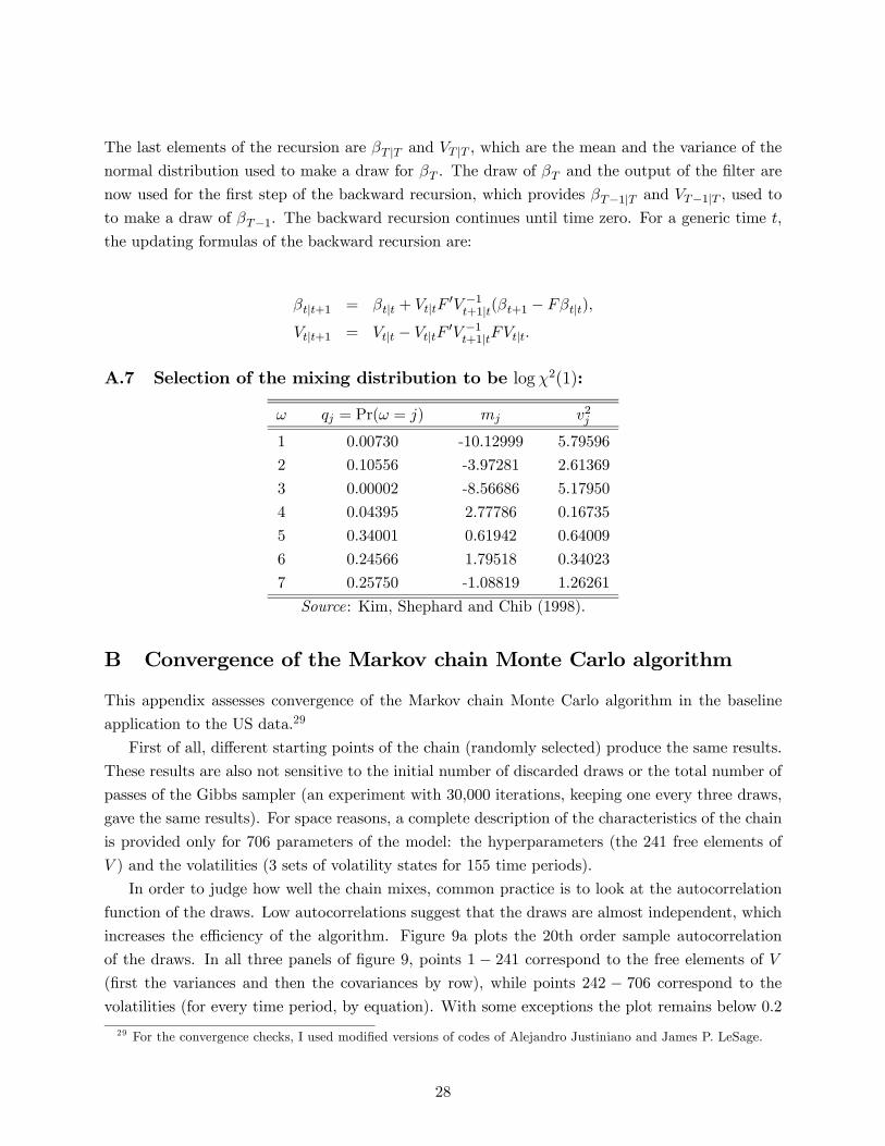
The last elements of the recursion are βT |T and VT |T , which are the mean and the variance of thenormal distribution used to make a draw for βT . The draw of βT and the output of the filter are

now used for the first step of the backward recursion, which provides βT−1|T and VT−1|T , used toto make a draw of βT−1. The backward recursion continues until time zero. For a generic time t,the updating formulas of the backward recursion are:

βt|t+1 = βt|t + Vt|tF 0V −1t+1|t(βt+1 − Fβt|t),

Vt|t+1 = Vt|t − Vt|tF 0V −1t+1|tFVt|t.

A.7 Selection of the mixing distribution to be logχ2(1):

ω qj = Pr(ω = j) mj v2j

1 0.00730 -10.12999 5.79596

2 0.10556 -3.97281 2.61369

3 0.00002 -8.56686 5.17950

4 0.04395 2.77786 0.16735

5 0.34001 0.61942 0.64009

6 0.24566 1.79518 0.34023

7 0.25750 -1.08819 1.26261

Source: Kim, Shephard and Chib (1998).

B Convergence of the Markov chain Monte Carlo algorithm

This appendix assesses convergence of the Markov chain Monte Carlo algorithm in the baseline

application to the US data.29

First of all, different starting points of the chain (randomly selected) produce the same results.

These results are also not sensitive to the initial number of discarded draws or the total number of

passes of the Gibbs sampler (an experiment with 30,000 iterations, keeping one every three draws,

gave the same results). For space reasons, a complete description of the characteristics of the chain

is provided only for 706 parameters of the model: the hyperparameters (the 241 free elements of

V ) and the volatilities (3 sets of volatility states for 155 time periods).

In order to judge how well the chain mixes, common practice is to look at the autocorrelation

function of the draws. Low autocorrelations suggest that the draws are almost independent, which

increases the efficiency of the algorithm. Figure 9a plots the 20th order sample autocorrelation

of the draws. In all three panels of figure 9, points 1 − 241 correspond to the free elements of V(first the variances and then the covariances by row), while points 242 − 706 correspond to thevolatilities (for every time period, by equation). With some exceptions the plot remains below 0.2

29 For the convergence checks, I used modified versions of codes of Alejandro Justiniano and James P. LeSage.

28

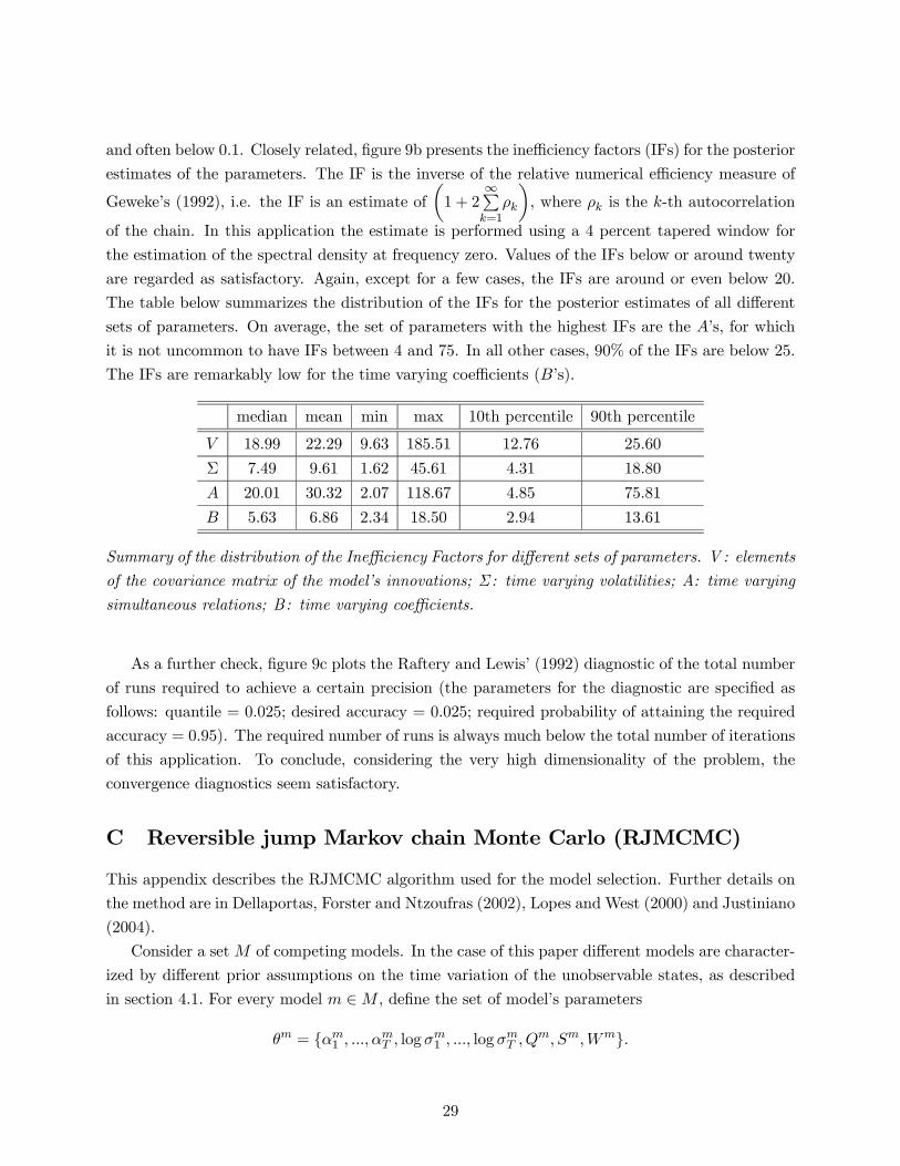
and often below 0.1. Closely related, figure 9b presents the inefficiency factors (IFs) for the posterior

estimates of the parameters. The IF is the inverse of the relative numerical efficiency measure of

Geweke’s (1992), i.e. the IF is an estimate ofµ1 + 2

∞Pk=1

ρk

¶, where ρk is the k-th autocorrelation

of the chain. In this application the estimate is performed using a 4 percent tapered window for

the estimation of the spectral density at frequency zero. Values of the IFs below or around twenty

are regarded as satisfactory. Again, except for a few cases, the IFs are around or even below 20.

The table below summarizes the distribution of the IFs for the posterior estimates of all different

sets of parameters. On average, the set of parameters with the highest IFs are the A’s, for which

it is not uncommon to have IFs between 4 and 75. In all other cases, 90% of the IFs are below 25.

The IFs are remarkably low for the time varying coefficients (B’s).

median mean min max 10th percentile 90th percentile

V 18.99 22.29 9.63 185.51 12.76 25.60

Σ 7.49 9.61 1.62 45.61 4.31 18.80

A 20.01 30.32 2.07 118.67 4.85 75.81

B 5.63 6.86 2.34 18.50 2.94 13.61

Summary of the distribution of the Inefficiency Factors for different sets of parameters. V : elements

of the covariance matrix of the model’s innovations; Σ : time varying volatilities; A: time varying

simultaneous relations; B : time varying coefficients.

As a further check, figure 9c plots the Raftery and Lewis’ (1992) diagnostic of the total number

of runs required to achieve a certain precision (the parameters for the diagnostic are specified as

follows: quantile = 0.025; desired accuracy = 0.025; required probability of attaining the required

accuracy = 0.95). The required number of runs is always much below the total number of iterations

of this application. To conclude, considering the very high dimensionality of the problem, the

convergence diagnostics seem satisfactory.

C Reversible jump Markov chain Monte Carlo (RJMCMC)

This appendix describes the RJMCMC algorithm used for the model selection. Further details on

the method are in Dellaportas, Forster and Ntzoufras (2002), Lopes and West (2000) and Justiniano

(2004).

Consider a setM of competing models. In the case of this paper different models are character-

ized by different prior assumptions on the time variation of the unobservable states, as described

in section 4.1. For every model m ∈M , define the set of model’s parameters

θm = αm1 , ..., αmT , log σm1 , ..., log σmT , Qm, Sm,Wm.

29

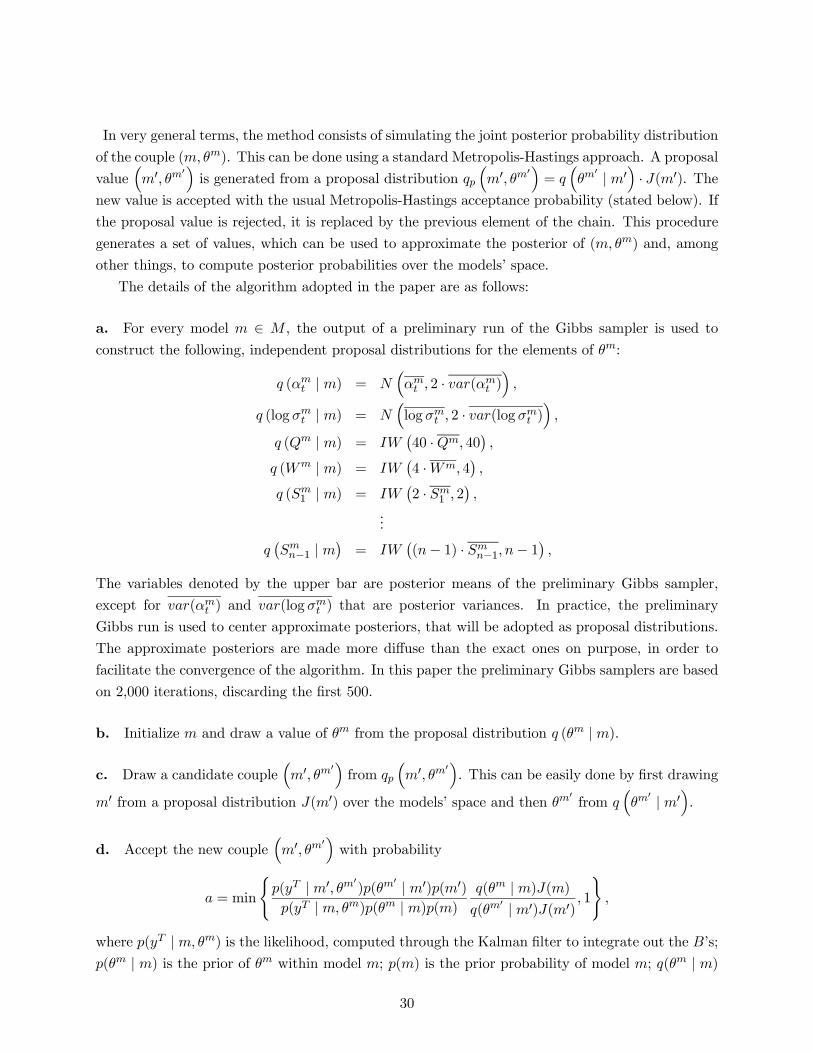
In very general terms, the method consists of simulating the joint posterior probability distribution

of the couple (m, θm). This can be done using a standard Metropolis-Hastings approach. A proposal

value³m0, θm

0´is generated from a proposal distribution qp

³m0, θm

0´= q

³θm

0 | m0´· J(m0). The

new value is accepted with the usual Metropolis-Hastings acceptance probability (stated below). If

the proposal value is rejected, it is replaced by the previous element of the chain. This procedure

generates a set of values, which can be used to approximate the posterior of (m, θm) and, among

other things, to compute posterior probabilities over the models’ space.

The details of the algorithm adopted in the paper are as follows:

a. For every model m ∈ M , the output of a preliminary run of the Gibbs sampler is used to

construct the following, independent proposal distributions for the elements of θm:

q (αmt | m) = N³αmt , 2 · var(αmt )

´,

q (log σmt | m) = N³log σmt , 2 · var(log σmt )

´,

q (Qm | m) = IW¡40 ·Qm, 40

¢,

q (Wm | m) = IW¡4 ·Wm, 4

¢,

q (Sm1 | m) = IW

¡2 · Sm

1 , 2¢,

...

q¡Smn−1 | m

¢= IW

¡(n− 1) · Sm

n−1, n− 1¢,

The variables denoted by the upper bar are posterior means of the preliminary Gibbs sampler,

except for var(αmt ) and var(log σmt ) that are posterior variances. In practice, the preliminary

Gibbs run is used to center approximate posteriors, that will be adopted as proposal distributions.

The approximate posteriors are made more diffuse than the exact ones on purpose, in order to

facilitate the convergence of the algorithm. In this paper the preliminary Gibbs samplers are based

on 2,000 iterations, discarding the first 500.

b. Initialize m and draw a value of θm from the proposal distribution q (θm | m).

c. Draw a candidate couple³m0, θm

0´from qp

³m0, θm

0´. This can be easily done by first drawing

m0 from a proposal distribution J(m0) over the models’ space and then θm0from q

³θm

0 | m0´.

d. Accept the new couple³m0, θm

0´with probability

a = min

(p(yT | m0, θm

0)p(θm

0 | m0)p(m0)p(yT | m, θm)p(θm | m)p(m)

q(θm | m)J(m)q(θm

0 | m0)J(m0), 1

),

where p(yT | m, θm) is the likelihood, computed through the Kalman filter to integrate out the B’s;

p(θm | m) is the prior of θm within model m; p(m) is the prior probability of model m; q(θm | m)

30

is the proposal distribution for the parameters, conditional on the model, constructed as above;

J(m) is the unconditional proposal distribution over the models. If the new draw is not accepted,

keep the previous couple (m, θm).

e. Go to c.

D The Markov chain Monte Carlo algorithm in the case of S un-restricted

This appendix presents an extension of the basic MCMC algorithm, in order to deal with the

case of S (the variance covariance matrix of the innovations to the simultaneous relations) left

unrestricted. The modification works as follows: step 2 of the Gibbs sampler is replaced by a

Metropolis-Hastings step in which a candidate value for the α’s, αT∗, is drawn from a proposal

distribution fP (αT | yT , BT ,ΣT , V ). The candidate value is accepted with probability equal to

min

½1,p(αT∗ | yT , BT ,ΣT , V )fP (α

T,−1 | yT , BT ,ΣT , V )

p(αT,−1 | yT , BT ,ΣT , V )fP (αT∗ | yT , BT ,ΣT , V )

¾,

where p(·) is the posterior of αT and αT,−1 represents the previous draw of αT in the chain. If thecandidate is rejected, αT is set to be αT,−1. Step 4 is modified straightforwardly in order to sampleS jointly and not in blocks. As in the Gibbs sampling case, this procedure allows to draw from

the exact joint posterior of the parameters. The last issue is related to the choice of the proposal

distribution. A natural candidate is the distribution used to sample αT under the assumption of S

block diagonal. Another possibility is to treat (erroneously) the state space form given by (16) and

(6) as linear and draw a candidate value for αT using the usual forward and backward recursions.

Clearly, if the proposal distribution is not close to the true density convergence can be much slower

than in the baseline case. In the context of the empirical application of this paper, with both the

proposal distributions suggested above, the acceptance rate was approximately 12 percent.

31

References

BERNANKE B. S. and I. MIHOV (1998), “Measuring Monetary Policy”, The Quarterly Journal

of Economics, 113, 869-902.

BLANCHARD O. and J. SIMON (2001), “The Long and Large Decline in U.S. Output Volatility”,

Brookings Papers on Economic Activity 1, 135-164.

BOIVIN J. (2001), “The Fed’s Conduct of Monetary Policy: Has It Changed and Does It Matter?”,

Columbia Business School, mimeo.

BOIVIN J. and M. GIANNONI (2003), “Has Monetary Policy Become More Effective?”, NBER

working paper no. 9459.

BULLARD J. and K. MITRA (2000), “Determinacy, Learnability, and Monetary Policy Inertia”,

working paper no. 200-030A, Federal Reserve Bank of St. Luis.

CARTER C. K. and R. KOHN (1994), “On Gibbs Sampling for State Space Models”, Biometrika,

81, 541-553.

CARLIN B. P. and S. CHIB (1995), “Bayesian Model Choice via Markov Chain Monte Carlo

Methods”, Journal of Royal Statistical Society B, 157, 473-484.

CANOVA F. (1993), “Modelling and Forecasting Exchange Rates with a Bayesian Time-Varying

Coefficient Model”, Journal of Economic Dynamics and Control, 17, 233-261.

CHIB S., F. NARDARI and N. SHEPHARD (2002), “Analysis of High Dimensional Multivariate

Stochastic Volatility Models”, Nuffield College, University of Oxford, mimeo.

CHRISTIANO L. J., M. EICHENBAUM and C. EVANS (1999), “Monetary Shocks: What Have

We Learned and To What End?”, in J. B. Taylor and M. Woodford (Eds.), Handbook of

Macroeconomics, Elsevier Science, North-Holland, New York, 1A, 65-148.

CICCARELLI M. and A. REBUCCI (2003), “Measuring Contagion with a Bayesian Time-Varying

Coefficient Model”, International Monetary Fund, mimeo.

COGLEY T. (2003), “How Fast Can the New Economy Grow? A Bayesian Analysis of the

Evolution of Trend Growth”, University of California, Davis, mimeo.

COGLEY T. and T.J. SARGENT (2001), “Evolving Post-World War II U.S. Inflation Dynamics”,

NBER Macroeconomics Annual, MIT Press, Cambridge, Massachusetts, 331-373.

COGLEY T. and T.J. SARGENT (2003), “Drifts and Volatilities: Monetary Policies and Out-

comes in the Post WWII U.S.”, New York University, mimeo.

32

COX D. R. and N. WERMUTH (1996), Multivariate Dependencies - Models, Analysis and Inter-

pretation, Chapman and Hall, London.

DELLAPORTAS P., J. J. FORSTER and I. NTZOUFRAS (2002), “On Bayesian Model and

Variable Selection Using MCMC”, Statistics and Computing, 12, 27-36.

DEMPSTER A. (1972), “Covariance Selection”, Biometrics, 28, 157-175.

DOUCET A., N. DE FREITAS and N. GORDON (2001), Sequential Monte Carlo Methods in

Practice, Springer-Verlag, New York.

FAVERO, C. A. and R. ROVELLI (2003), “Macroeconomic Stability and the Preferences of the

Fed. A Formal Analysis, 1961-1998”, Journal of Money, Credit and Banking, 35(4), 545-556.

FRUHWIRTH-SCHNATTER S. (1994), “Data Augmentation and Dynamic Linear Models”, Jour-

nal of Time Series Analysis, 15, 183-202.

GELMAN A., J. B. CARLIN, H. S. STERN and D. B. RUBIN (1995), Bayesian Data Analysis,

Chapman and Hall, London.

GEWEKE J. (1992), “Evaluating the Accuracy of Sampling-Based Approaches to the Calculation

of Posterior Moments”, in J. M. Bernardo, J. Berger, A. P. Dawid and A. F. M. Smith (Eds.),

Bayesian Statistics, Oxford University Press, Oxford, 169-193.

HAMILTON J. H. (1989), “A New Approach to the Economic Analysis of Nonstationary Time

Series and the Business Cycle”, Econometrica, 57(2), 357-384.

HANSON M. (2003), “Varying Monetary Policy Regimes: a Vector Autoregressive Investigation”,

Wesleyan University, mimeo.

HARVEY A. C., E. RUIZ and N. SHEPHARD (1994), “Multivariate Stochastic Variance Models”,

Review of Economic Studies, 61, 247-264.

JACQUIER E., N. G. POLSON and P. E. ROSSI (1994), “Bayesian Analysis of Stochastic Volatil-

ity Models”, Journal of Business and Economic Statistics, 12, 371-417.

JACQUIER E., N. G. POLSON and P. E. ROSSI (1995), “Models and Priors for Multivariate

Stochastic Volatility”, CIRANO working paper, 1995-18.

JUDD J. and G. D. RUDEBUSCH (1998), “Taylor’s Rule and the Fed: 1970-1997”, Federal

Reserve Bank of San Francisco Economic Review, 3, 3-16.

JUSTINIANO A. (2004), “Estimation and Model Selection in Dynamic Factor Analysis”, Inter-

national Monetary Fund, mimeo.

33

KIM C. and C. R. NELSON (1999), State-Space Models with Regime Switching, MIT Press,

Cambridge, Massachusetts.

KIM S., N. SHEPHARD and S. CHIB (1998),“Stochastic Volatility: Likelihood Inference and

Comparison with ARCH Models”, Review of Economic Studies, 65, 361-393.

LEEPER E. and T. ZHA (2002), “Modest Policy Intervention”, NBER working paper no. 9192.

LEEPER E., C. A. SIMS and T. ZHA (1996), “What Does Monetary Policy Do?”, Brookings

Papers on Economic Activity 2, 1-78.

LOPES H. F. and M. WEST (2000), “Model Uncertainty in Factor Analysis”, Duke University,

mimeo.

LUBIK T. A. and F. SCHORFHEIDE (2004), “Testing for Indeterminacy: An Application to

U.S. Monetary Policy”, American Economic Review, 94(1), 190-217.

LUCAS R. E. (1976), “Econometric Policy Evaluation: a Critique”, in K. Brunner and A. Meltzer

(Eds.) The Phillips Curve and Labor Markets, Canergie-Rochester Series on Public Policy, 1,

19-46.

PINHEIRO J. and D. BATES (1996), “Unconstrained Parametrizations for Variance-Covariance

Matrices”, Statistics and Computing, 11, 289-296.

POURAHMADI M. (1999), “Joint Mean-Covariance Models with Applications to Longitudinal

Data: Unconstrained Parameterizations”, Biometrika, 86, 677-690.

POURAHMADI M. (2000), “Maximum Likelihood Estimation for Generalized Linear Models for

Multivariate Normal Covariance Matrices”, Biometrika, 87, 425-435.

RAFTERY A. E. and S. LEWIS (1992), “How Many Iterations in the Gibbs Sampler?” in J. M.

Bernardo, J. Berger, A. P. Dawid and A. F. M. Smith (Eds.), Bayesian Statistics, Oxford

University Press, Oxford, 763-773.

ROTEMBERG J. J. and M. WOODFORD (1997), “An Optimization-Based Econometric Frame-

work for the Evaluation of Monetary Policy”, NBER Macroeconomics Annual, MIT Press,

Cambridge, Massachusetts, 297-346.

SARGAN J. D. and A. BHARGAVA (1983), “Maximum Likelihood Estimation of Regression

Models with First Order Moving Average Errors when the Root Lies on the Unit Circle”,

Econometrica, 51, 799-820.

SHEPHARD N. (1994a), “Local Scale Models: State Space Alternatives to Integrated GARCH

Processes”, Journal of Econometrics, 60, 181-202.

SHEPHARD N. (1994b), “Partial Non-Gaussian State Space”, Biometrika, 81, 115-131.

34

SHEPHARD N. (1996), “Statistical Aspects of ARCH and Stochastic Volatility”, in D. R. Cox, D.

V. Hinkley and O. E. Barndorff-Nielsen (Eds.), Time Series Models in Econometrics, Finance

and Other Fields, Chapman and Hall, London, 1-67.

SHEPHARD N. and A. C. HARVEY (1990), “On the Probability of Estimating a Deterministic

Component in the Local Level Model”, Journal of Time Series Analysis, 11(4), 339-347.

SIMS C. A. (1993), “A 9 Variable Probabilistic Macroeconomic Forecasting Model”, in J. H.

Stock and M. W. Watson (Eds.), Business Cycles, Indicators and Forecasting, NBER studies

in business cycles volume 28, 179-214.

SIMS C. A. (1999), “Drift and Breaks in Monetary Policy”, Princeton University, mimeo.

SIMS C. A. (2000), “Using a Likelihood Perspective to Sharpen Econometric Discourse: Three

Examples”, Journal of Econometrics, 95(2), 443-462.

SIMS C. A. (2001a), “Stability and instability in US monetary policy behavior”, Princeton Uni-

versity, mimeo.

SIMS C. A. (2001b), “Comment on Sargent and Cogley’s: ‘Evolving Post World War II U.S. In-

flation Dynamics”’, NBER Macroeconomics Annual, MIT Press, Cambridge, Massachusetts,

373-379.

SIMS C. A. and T. ZHA (1998), “Bayesian Methods for Dynamics Multivariate Models”, Inter-

national Economic Review, 39, 949-968.

SIMS C. A. and T. ZHA (2004), “Were There Regime Switches in USMonetary Policy?”, Princeton

University, mimeo.

SMITH M. and R. KOHN (2002), “Parsimonious Covariance Matrix Estimation for Longitudinal

Data”, Journal of the American Statistical Association, 97, 1141-1153.

STOCK J. H. and M. W. WATSON (1996), “Evidence on Structural Instability in Macroeconomic

Time Series Relations”, Journal of Business and Economic Statistics, 14, 11-30.

STOCK J. H. and M. W. WATSON (1998), “Asymptotically Median Unbiased Estimation of

Coefficient Variance in a Time Varying Parameter Model”, Journal of the American Statistical

Association, 93, 349-358.

STOCK J. H. and M. W. WATSON (2001), “Vector Autoregressions”, Journal of Economic

Perspectives, 15, 101-116.

STOCK J. H. and M. W. WATSON (2002), “Has the Business Cycle Changed and Why?”, NBER

working paper no. 9127.

35

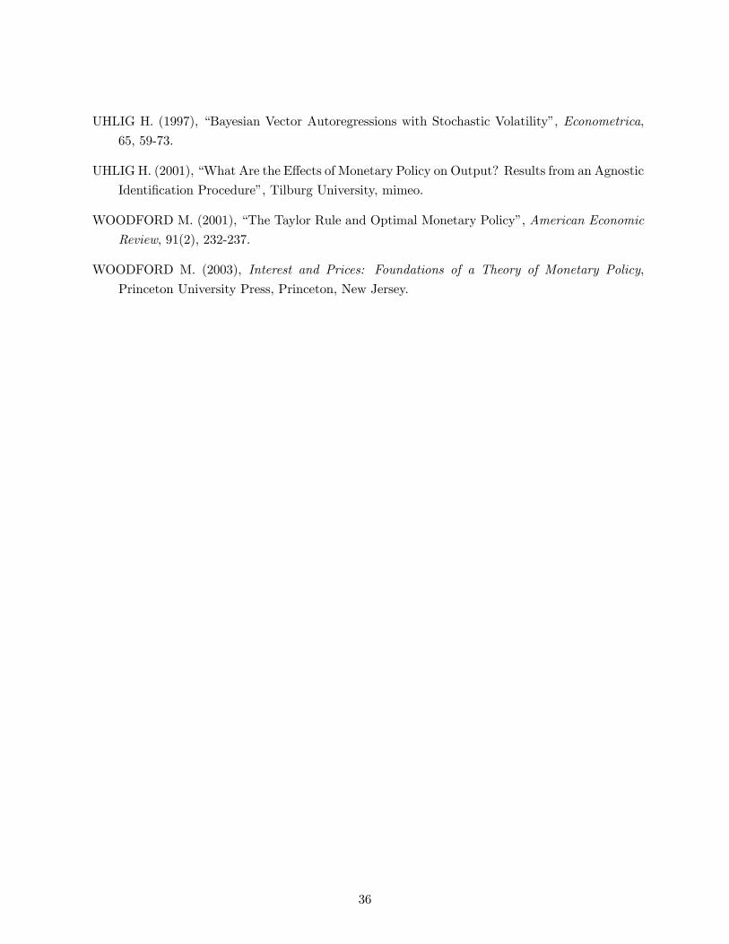
UHLIG H. (1997), “Bayesian Vector Autoregressions with Stochastic Volatility”, Econometrica,

65, 59-73.

UHLIG H. (2001), “What Are the Effects of Monetary Policy on Output? Results from an Agnostic

Identification Procedure”, Tilburg University, mimeo.

WOODFORD M. (2001), “The Taylor Rule and Optimal Monetary Policy”, American Economic

Review, 91(2), 232-237.

WOODFORD M. (2003), Interest and Prices: Foundations of a Theory of Monetary Policy,

Princeton University Press, Princeton, New Jersey.

36

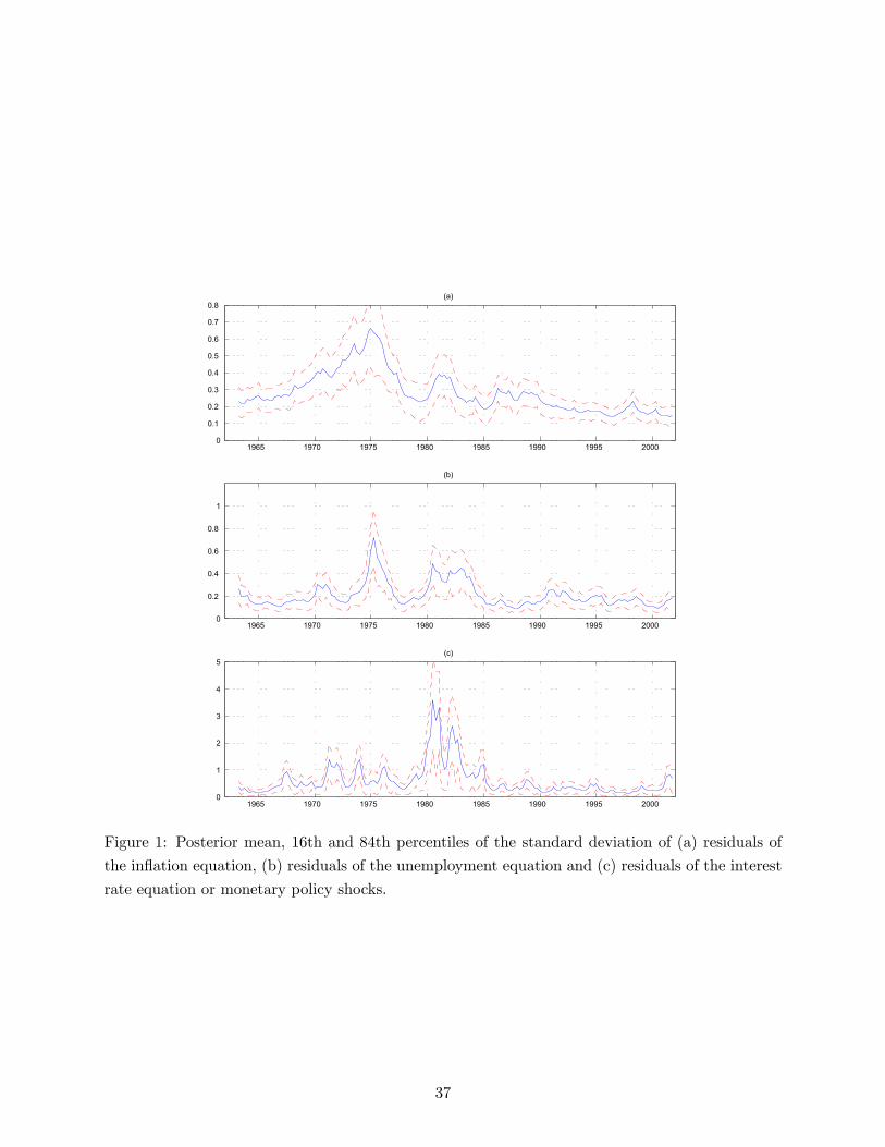
1965 1970 1975 1980 1985 1990 1995 20000

0.1

0.2

0.3

0.4

0.5

0.6

0.7

0.8(a)

1965 1970 1975 1980 1985 1990 1995 20000

0.2

0.4

0.6

0.8

1

(b)

1965 1970 1975 1980 1985 1990 1995 20000

1

2

3

4

5(c)

Figure 1: Posterior mean, 16th and 84th percentiles of the standard deviation of (a) residuals of

the inflation equation, (b) residuals of the unemployment equation and (c) residuals of the interest

rate equation or monetary policy shocks.

37

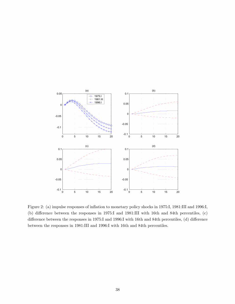
0 5 10 15 20

-0.1

-0.05

0

0.05(a)

1975:I1981:III1996:I

0 5 10 15 20-0.1

-0.05

0

0.05

0.1(b)

0 5 10 15 20-0.1

-0.05

0

0.05

0.1(c)

0 5 10 15 20-0.1

-0.05

0

0.05

0.1(d)

Figure 2: (a) impulse responses of inflation to monetary policy shocks in 1975:I, 1981:III and 1996:I,

(b) difference between the responses in 1975:I and 1981:III with 16th and 84th percentiles, (c)

difference between the responses in 1975:I and 1996:I with 16th and 84th percentiles, (d) difference

between the responses in 1981:III and 1996:I with 16th and 84th percentiles.

38

0 5 10 15 20

-0.02

0

0.02

0.04

0.06

0.08

0.1

(a)

1975:I1981:III1996:I

0 5 10 15 20-0.1

-0.05

0

0.05

0.1(b)

0 5 10 15 20-0.1

-0.05

0

0.05

0.1(c)

0 5 10 15 20-0.1

-0.05

0

0.05

0.1(d)

Figure 3: (a) impulse responses of unemployment to monetary policy shocks in 1975:I, 1981:III and

1996:I, (b) difference between the responses in 1975:I and 1981:III with 16th and 84th percentiles, (c)

difference between the responses in 1975:I and 1996:I with 16th and 84th percentiles, (d) difference

between the responses in 1981:III and 1996:I with 16th and 84th percentiles.

39

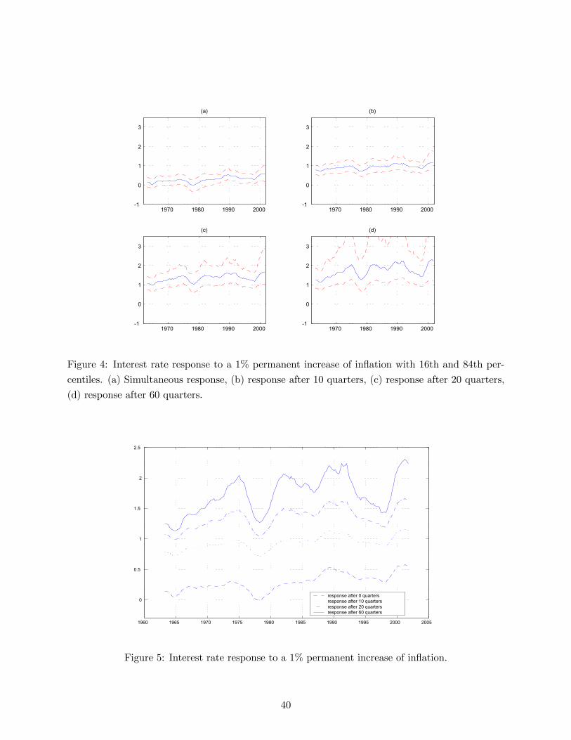
1970 1980 1990 2000-1

0

1

2

3

(a)

1970 1980 1990 2000-1

0

1

2

3

(b)

1970 1980 1990 2000-1

0

1

2

3

(c)

1970 1980 1990 2000-1

0

1

2

3

(d)

Figure 4: Interest rate response to a 1% permanent increase of inflation with 16th and 84th per-

centiles. (a) Simultaneous response, (b) response after 10 quarters, (c) response after 20 quarters,

(d) response after 60 quarters.

1960 1965 1970 1975 1980 1985 1990 1995 2000 2005

0

0.5

1

1.5

2

2.5

response after 0 quartersresponse after 10 quartersresponse after 20 quartersresponse after 60 quarters

Figure 5: Interest rate response to a 1% permanent increase of inflation.

40

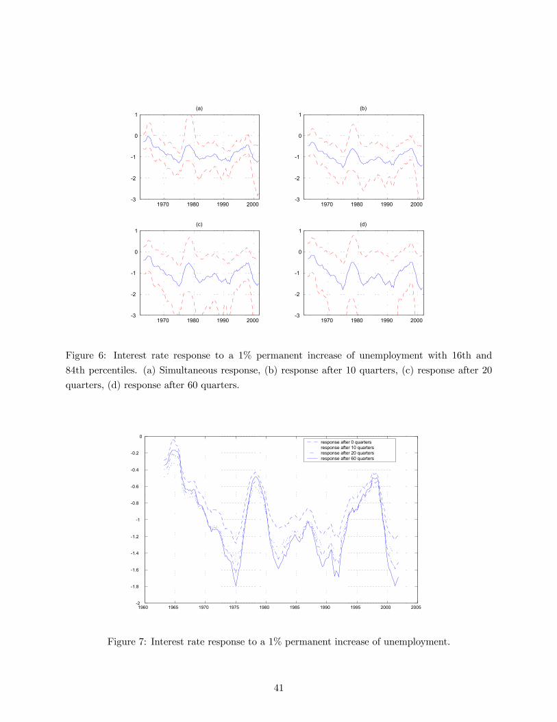
1970 1980 1990 2000-3

-2

-1

0

1(a)

1970 1980 1990 2000-3

-2

-1

0

1(b)

1970 1980 1990 2000-3

-2

-1

0

1(c)

1970 1980 1990 2000-3

-2

-1

0

1(d)

Figure 6: Interest rate response to a 1% permanent increase of unemployment with 16th and

84th percentiles. (a) Simultaneous response, (b) response after 10 quarters, (c) response after 20

quarters, (d) response after 60 quarters.

1960 1965 1970 1975 1980 1985 1990 1995 2000 2005-2

-1.8

-1.6

-1.4

-1.2

-1

-0.8

-0.6

-0.4

-0.2

0response after 0 quartersresponse after 10 quartersresponse after 20 quartersresponse after 60 quarters

Figure 7: Interest rate response to a 1% permanent increase of unemployment.

41

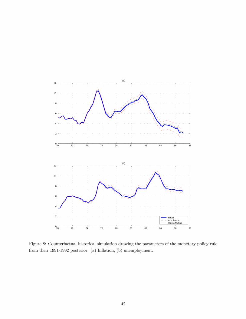
70 72 74 76 78 80 82 84 86 880

2

4

6

8

10

12(a)

70 72 74 76 78 80 82 84 86 880

2

4

6

8

10

12(b)

actualerror bandscounterfactual

Figure 8: Counterfactual historical simulation drawing the parameters of the monetary policy rule

from their 1991-1992 posterior. (a) Inflation, (b) unemployment.

42

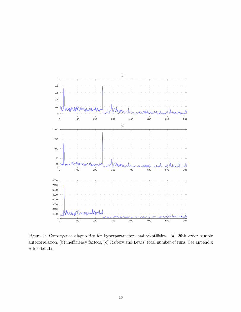
0 100 200 300 400 500 600 700

0

0.2

0.4

0.6

0.8

1(a)

0 100 200 300 400 500 600 7000

20

50

100

150

200

(b)

0 100 200 300 400 500 600 7000

1000

2000

3000

4000

5000

6000

7000

8000

(c)

Figure 9: Convergence diagnostics for hyperparameters and volatilities. (a) 20th order sample

autocorrelation, (b) inefficiency factors, (c) Raftery and Lewis’ total number of runs. See appendix

B for details.

43