Timescale Analysis with an Entropy-Based Shift-Invariant Discrete Wavelet Transform

Comput EconDOI 10.1007/s10614-013-9381-z

Timescale Analysis with an Entropy-BasedShift-Invariant Discrete Wavelet Transform

Stelios D. Bekiros

Accepted: 2 May 2013© Springer Science+Business Media New York 2013

Abstract This paper presents an invariant discrete wavelet transform that enablespoint-to-point (aligned) comparison among all scales, contains no phase shifts, relaxesthe strict assumption of a dyadic-length time series, deals effectively with boundaryeffects and is asymptotically efficient. It also introduces a new entropy-based method-ology for the determination of the optimal level of the multiresolution decomposition,as opposed to subjective or ad-hoc approaches used hitherto. As an empirical appli-cation, the paper relies on wavelet analysis to reveal the complex dynamics acrossdifferent timescales for one of the most widely traded foreign exchange rates, namelythe Great Britain Pound. The examined period covers the global financial crisis and theEurozone debt crisis. The timescale analysis attempts to explore the micro-dynamicsof across-scale heterogeneity in the second moment (volatility) on the basis of marketagent behavior with different trading preferences and information flows across scales.New stylized properties emerge in the volatility structure and the implications for theflow of information across scales are inferred.

Keywords Wavelets · Entropy · Exchange rates

JEL Classification C14 · C32 · C51 · F31

S. D. Bekiros (B)Department of Economics, European University Institute, Via della Piazzuola 43, 50133 Florence, Italye-mail: [email protected]

S. D. BekirosDepartment of Accounting and Finance, Athens University of Economics and Business,76, Patission str., 10434 Athens, Greecee-mail: [email protected]

S. D. BekirosRimini Centre for Economic Analysis (RCEA), Via Patara, 3, 47900 Rimini, Italy

123

S. D. Bekiros

1 Introduction

In contrast to the classical Fourier analysis, in which the frequency content of theunderlying time series is assumed to be stationary along the time axis, wavelets aredefined over a finite domain and unlike the Fourier transform they are localized both intime and in scale. This property, as opposed to the trigonometric or complex exponen-tial functions in Fourier transform, makes wavelets ideal for analysing nonstationarysignals especially those incorporating transient phenomena or singularities. Waveletanalysis works with “translates” and “dilates” of a single local function, the so-called“mother wavelet”, which is locally defined with compact support or decays suffi-ciently fast. However, the existence of wavelets is not a trivial analytical issue and theconstruction of classes of compactly supported wavelets was first addressed byDaubechies (1988). In that work a reliable methodology for obtaining orthogonalwavelet bases by translating and dilating the mother wavelet was provided. As amother wavelet with compact support is located in a finite interval, the analysis of asingularity is performed by considering only those translates of the mother wavelet thatoverlap the singularity. Daubechies (1988) contribution was followed by the devel-opment of multiresolution analysis by Mallat (1989) and Coifman and Wickerhauser(1992).

Technically, Fourier and wavelet methods involve the projection of a signal ontoan orthonormal set of components. Fourier projections are most naturally definedfor functions restricted to L2(0, 2π) i.e., the set of square integrable functions inthe interval (0, 2π), because Fourier series have infinite energy but finite power whenextended to being defined over the entire real axis. Based on the complex superpositionof individual harmonics, the hypothesis is that over any segment of the time series theexact same frequencies hold at the same amplitudes, namely the signal is homogeneousover time. On the contrary, the basis functions in wavelet analysis are defined inL2(R) and are not necessarily homogeneous over time, meaning that they have narrowcompact support so that they rapidly converge to zero as time approaches infinity.Such basis functions are called wavelets, in distinction to the trigonometric functionstraditionally associated with waves.

The flurry of interest in economic applications of wavelets emerged in the mid-90s mostly by Ramsey and his collaborators. Ramsey et al. (1995) pursued a waveletapproach in detecting self-similarity in US stock prices. In addition, Ramsey and Lam-part (1998a,b) used a wavelet-based scaling method to investigate the relationship andcausality between money, income and expenditure. In other studies Goffe (1994) illus-trated the application of wavelets to nonstationary macroeconomic data, in particularfor the detection of discontinuities and the occurrence of sharp cusps. In recent works,Almasri and Shukur (2003) address the causal relation between spending and revenueat different timescales, while Gençay et al. (2002) look into dependencies betweenmoney, income, expenditure, growth and inflation. Fernandez (2005) deals with theestimation of systematic asset risk. Finally, it is also worth mentioning a stream ofpapers utilizing wavelet methodology to address theoretical econometric issues anddevise new statistical approaches Lee J. and Y. Hong (2001).

123

Shift-Invariant Discrete Wavelet Transform

1.1 Time Scaling in Economics Revisited

In natural sciences the utilization of sequences of timescales in the analysis of differentmodes of behavior, or different relationships between variables, is very common. Ineconomics the notion of timescale is related to time period segmentation and theexamined relationships are described as short-run and long-run, or broadly under theterm scaling laws (Brock 1999). The scale decomposition often reveals the presence ofdeterministic regularities or statistical properties of the conditional moments that areseemingly independent of the scale details. However, in wavelet literature the conceptof time scaling or “dilation” is quite different from that in economics. The differentscales of the wavelet decomposition contain contributions of the signal in differentfrequencies (although timescale and frequency are not identical concepts as it is furtherexplained below). Based on the selected function space, the time series are analysedinto “fine” and “coarse” resolution components extracted from the application of“father” and “mother” wavelets. The former represent the smooth and low-frequencyparts of a signal, whereas the latter incorporate the detailed and high-frequency features(Percival and Walden 2000).

While frequency analysis (Fourier) results in projecting the entire signal ontoever lower frequencies, time scaling with wavelets is concerned with projecting alocalized component of the signal onto an increasingly broader base. Moreover, thebasis functions are orthogonal across scales, so that the total variation/energy ofthe signal at any given point in time is obtained by adding the constituent com-ponents extracted at each of the scales. Although at first sight timescale coulddirectly correspond to frequency there is only an indirect connection between thesetwo concepts, as indicated by Priestley (1996). Intuitively, in a naïve interpreta-tion, wide-support wavelets can be associated with low frequencies, while high-frequency analysis requiring high sampling rates can be provided by narrow-supportcomponents.

The multiresolution features of wavelet decomposition can be useful in econometricanalysis. Through wavelet decomposition, the low-frequency content of the data that“captures” the true dynamic relationships can be extracted and the high-frequencyfluctuations that might distort the underlying dependencies of the economy can beremoved. This paper contributes to the literature by introducing an invariant transformthat enables point-to-point comparison among all scales, contains no phase shifts,relaxes the strict assumption of a “dyadic-length” time series, deals effectively with“boundary effects” and is asymptotically efficient. In addition, beyond the existingpractice that has utilized subjective judgment in considering the appropriate “depth”of the wavelet analysis, a new entropy-based methodology is introduced to determinethe optimal level of decomposition. Finally, an empirical application in financial timeseries—in particular exchange rates—is pursued. These series are inherently charac-terized by chaotic patterns, fat tails and long-memory, particularly at high samplingfrequencies. The results provide evidence of complex heterogeneous dynamics acrossand within different scales.

The paper develops as follows: Sect. 2 provides an overview of multiresolutionmethodology and presents a new shift-invariant discrete wavelet transform. Finally,Sect. 3 provides an empirical application and Sect. 4 the concluding remarks.

123

S. D. Bekiros

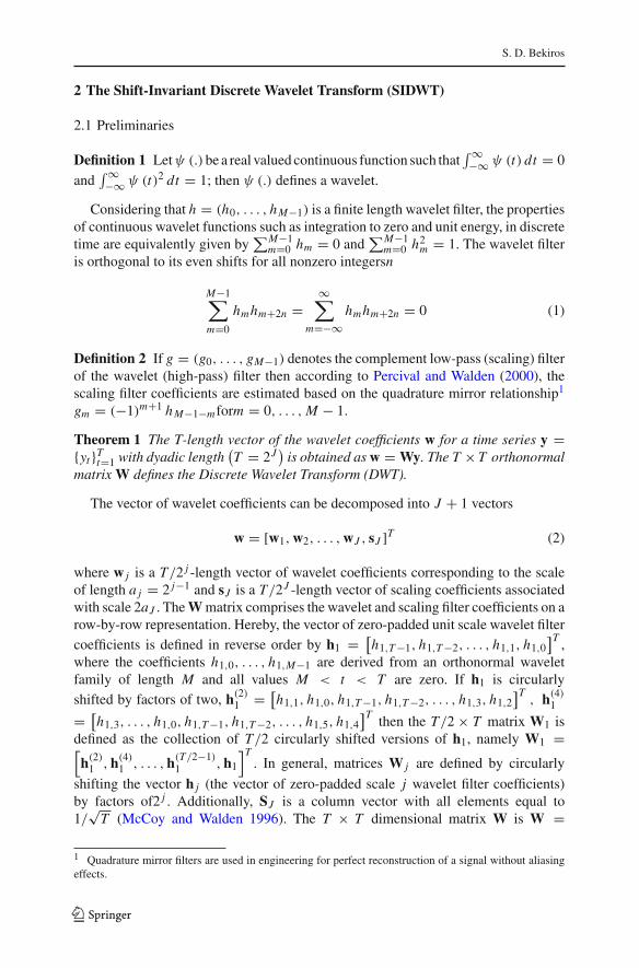
2 The Shift-Invariant Discrete Wavelet Transform (SIDWT)

2.1 Preliminaries

Definition 1 Letψ (.)be a real valued continuous function such that∫ ∞−∞ ψ (t) dt = 0

and∫ ∞−∞ ψ (t)2 dt = 1; then ψ (.) defines a wavelet.

Considering that h = (h0, . . . , hM−1) is a finite length wavelet filter, the propertiesof continuous wavelet functions such as integration to zero and unit energy, in discretetime are equivalently given by

∑M−1m=0 hm = 0 and

∑M−1m=0 h2

m = 1. The wavelet filteris orthogonal to its even shifts for all nonzero integersn

M−1∑

m=0

hmhm+2n =∞∑

m=−∞hmhm+2n = 0 (1)

Definition 2 If g = (g0, . . . , gM−1) denotes the complement low-pass (scaling) filterof the wavelet (high-pass) filter then according to Percival and Walden (2000), thescaling filter coefficients are estimated based on the quadrature mirror relationship1

gm = (−1)m+1 hM−1−mform = 0, . . . ,M − 1.

Theorem 1 The T-length vector of the wavelet coefficients w for a time series y ={yt }T

t=1 with dyadic length(T = 2J

)is obtained as w = Wy. The T × T orthonormal

matrix W defines the Discrete Wavelet Transform (DWT).

The vector of wavelet coefficients can be decomposed into J + 1 vectors

w = [w1,w2, . . . ,wJ , sJ ]T (2)

where w j is a T/2 j -length vector of wavelet coefficients corresponding to the scaleof length a j = 2 j−1 and sJ is a T/2J -length vector of scaling coefficients associatedwith scale 2aJ . The W matrix comprises the wavelet and scaling filter coefficients on arow-by-row representation. Hereby, the vector of zero-padded unit scale wavelet filtercoefficients is defined in reverse order by h1 = [

h1,T −1, h1,T −2, . . . , h1,1, h1,0]T ,

where the coefficients h1,0, . . . , h1,M−1 are derived from an orthonormal waveletfamily of length M and all values M < t < T are zero. If h1 is circularlyshifted by factors of two, h(2)1 = [

h1,1, h1,0, h1,T −1, h1,T −2, . . . , h1,3, h1,2]T, h(4)1

= [h1,3, . . . , h1,0, h1,T −1, h1,T −2, . . . , h1,5, h1,4

]T then the T/2 × T matrix W1 isdefined as the collection of T/2 circularly shifted versions of h1, namely W1 =[h(2)1 ,h(4)1 , . . . ,h(T/2−1)

1 ,h1

]T. In general, matrices W j are defined by circularly

shifting the vector h j (the vector of zero-padded scale j wavelet filter coefficients)by factors of2 j . Additionally, SJ is a column vector with all elements equal to1/

√T (McCoy and Walden 1996). The T × T dimensional matrix W is W =

1 Quadrature mirror filters are used in engineering for perfect reconstruction of a signal without aliasingeffects.

123


[W1W2 . . .WJ SJ ]T . From matrix W the wavelet filter coefficients for scales 1, . . . , Jare computed via the Inverse Discrete Fourier Transform (IDFT). Specifically, giventhe transfer functions of the wavelet (Hj,k) and scaling filters (G J,k), the wavelet forscale a j = 2 j−1 is estimated as the inverse DFT2

h j,l =F−1 {Hj,k

}=F−1

⎧⎨

⎩H1,2 j−1k mod T

j−2∏

l=0

G1,2m k mod T

⎫⎬

⎭, k =0, . . . , T −1 (3)

with length M j = (2 j − 1

)(M − 1) + 1. In the same way, the scaling filter gJ for

scale aJ is derived as the inverse DFT of G J,k

gJ,l = F−1 {G J,k

} = F−1

{

G J,k =J−1∏

l=0

G1,2m k mod T

}

, k = 0, . . . , T − 1 (4)

Mallat (1989) introduced the “pyramid algorithm” for the implementation of the DWT.The following proposition proves how the coefficients are produced.

Proposition 1 In the Mallat algorithm the data yt are filtered using h1 and g1, thenthe outputs are subsampled to half their original lengths and the subsampled filteroutput from h1 accounts for the wavelet coefficients. This process is repeated on thesubsampled output from g1 filter.

The first step of the pyramid algorithm begins by convolving the data with eachfilter to obtain the following wavelet w1,t = ∑M−1

m=0 hm y2t+1−m mod T and scalingcoefficients s1,t = ∑M−1

m=0 gm y2t+1−m mod T where t = 0, 1, . . . , T/2 − 1. This alsoincludes a downsampling operation, in that every other value of the input vector isremoved. Consequently, the T -length vector of observations has been high-and low-pass filtered to obtain T/2 coefficients. The second step of the algorithm starts by“initializing” the sample now to be the scaling coefficients s1 and apply the aforemen-tioned filtering procedure to obtain the second level of wavelet and scaling coefficientsasw2,t = ∑M−1

m=0 hms1,2t+1−m mod T and s2,t = ∑M−1m=0 gms1,2t+1−m mod T respectively

with t = 0, 1, . . . , T/4 − 1. By saving all wavelet coefficients and the final level ofscaling coefficients the decomposition becomes w = [w1w2s2]T . This procedure isrepeated up to J = log2 (T ) times and provides the vector of wavelet coefficients inEq. (2).

The inversion of the DWT is performed by upsampling the final wavelet and scalingcoefficients, convolving them with their respective filters and adding the resultingvectors. Upsampling the vectors wJ and sJ of the final DWT level produces the newvectors w0

J = [0wJ,0

]T and s0J = [

0sJ,0]T . Now the vector of scaling coefficients sJ−1

is given by sJ−1,t = ∑M−1m=0 hmw

0J,t+m mod 2+

∑M−1m=0 gms0

J,t+m mod 2 with t = 0, 1 andit is twice that of sJ . This is repeated until the first level of all coefficients has beenupsampled, in order to produce the original vector of data observations, i.e.,

2 The modulus operator is required in order to deal with the boundary of a finite length vector of observa-tions.

123

S. D. Bekiros

yt =M−1∑

m=0

hmw01,t+m mod T +

M−1∑

m=0

gms01,t+m mod T t = 0, 1, . . . , T − 1.

The DWT results in the additive decomposition of the time series. The most impor-tant feature of the multiresolution analysis is the reverse process of signal synthesis.

Proposition 2 Let D j = WTj w j define the wavelet detail corresponding to changes

in the series y at scale a j for the level j = 1, . . . , J . The coefficients w j = W j yrepresent the part of the signal due to wavelet analysis at scale a j , while WT

j w j isthe part of the wavelet synthesis attributable to scale a j .

The final wavelet detail DJ+1 = STJ SJ is equal to the sample mean of the T = 2J

observations (Gençay et al. 2002). The multiresolution analysis is defined for eachobservation yt as the linear combination of wavelet detail coefficients, i.e., yt =∑J+1

j=1 D j,t t = 0, . . . , T − 1. Similarly, A j = ∑J+1k= j+1 Dk is the cumulative sum of

the variations of the details and is defined as the j-th level wavelet approximationfor 0 ≤ j ≤ J with AJ+1 being a vector of zeros. The j-th level wavelet roughR j = ∑ j

k=1 Dk, 1 ≤ j ≤ J + 1 incorporates the remaining lower-scale detailswhere R0 is the zero vector. Overall, the vector of observations may be decomposedfor all j through a wavelet approximation and rough as

y = A j +j∑

k=1

D j = A j + R j (5)

Definition 3 Orthonormality of the matrix W implies, as in case of DFT, that the DWT

is an efficient, variance preserving transform3,4 i.e., ‖w‖2 = ∑Jj=1

∑T/2 j −1t=0 w2

j,t

+s2J,0 = ∑T −1

t=0 x2t = ‖y‖2.

Consequently, the energy ‖y‖2 is decomposed on a scale-by-scale basis as ‖y‖2 =∑J

j=1

∥∥w j

∥∥2 + ‖sJ ‖2, where

∥∥w j

∥∥2 is the energy of y attributed to variance at scale

a j , and ‖sJ ‖2 is the remaining energy in aJ scales or higher. As DTj D j = wT

j w j and

ATJ AJ = sT

J sJ apply for 1 ≤ j ≤ J (due to orthonormality of W and S), an equal

decomposition is ‖y‖2 = ∑Jj=1

∥∥D j

∥∥2 + ‖AJ ‖2.

2.2 Formal Description of the SIDWT

The classical (decimated) DWT involves subsampling of the filter output to half theoriginal length. This leads to a serious drawback, namely the transform is not invariantin the real-axis. Specifically, the DWT of a shifted signal is not the shifted version

3 The energy of a vector—proportionate to variance—is defined as the sum of its squared coefficients.4 It can be also proven via matrix operations: ‖y‖2 = yT y = (Ww)T Ww = wT WT Ww = wT w =‖w‖2.

123


of the DWT of the signal.5 Alternatively, an undecimated DWT can be implementedwithout the subsampling technique. According to Coifman and Donoho (1995) undec-imated versions of the DWT could handle any sample size T , while the J-th orderDWT restricts the sample size to a multiple of 2J . Moreover, they are invariant tocircularly shifting the time series, a property that does not hold for the DWT. Finally,an undecimated wavelet variance estimator is asymptotically more efficient than theDWT estimator (Percival 1995). Hence, in this study a new variation of the undeci-mated DWT, namely the Shift-Invariant DWT (SIDWT) is proposed via the followingtheorem.

Theorem 2 The SIDWT is defined as follows: Let y be an arbitrary T - length vectorof observations. The (J + 1) T - length vector of SIDWT coefficients w is obtained asw = Wy, where w is a (J + 1) T × T matrix. The SIDWT coefficient vector, as inDWT, is organized into J + 1 vectors

w = [w1, w2, . . . , wJ , sJ

]T (6)

Let w j is a T/2 j - length vector of wavelet coefficients associated with the scaleof length a j = 2 j−1 and sJ is a T/2J - length vector of scaling coefficients corre-sponding to a length scale of 2J = 2aJ . The direct conversion to DWT could beimplemented for a dyadic length

(T = 2J

)sample, via subsampling and rescaling of

the SIDWT. The converted DWT wavelet coefficients are w j,t = 2 j/2w j,2 j (t+1)−1

with t = 0, . . . , T/2 j − 1, and the scaling coefficients sJ,t = 2J/2sJ,2J (t+1)−1t =0, . . . , T/2J − 1. In correspondence to the orthonormal matrix of the DWT, theSIDWT matrix W comprises J + 1 submatrices of T × T dimension expressed

as w =[w1w2 . . . wJ SJ

]T. The SIDWT utilizes the rescaled filters from DWT,

h j = h j/2 j and gJ = gJ /2J with ( j = 1, . . . , J ). The T × T submatrix w1 isconstructed by circularly shifting the rescaled wavelet filter vector h1 by integer units

to the right, i.e., w1 =[h(1)1 , h(2)1 , h(3)1 , . . . , h(T −2)

1 , h(T −1)1 , h1

]Tand it can be inter-

preted as the circularly shifted version of DWT submatrix W1. The other matricesw2, . . . , wJ are similarly constructed through replacing h1 by h j .

Proposition 3 The new implementation algorithm starts with the data yt , which is nolonger limited to dyadic length, and filters with h1 and g1 to obtain the T -length vectorsof wavelet and scaling coefficients w1 and s1, yet without utilizing the downsamplingoperation.

In the first step the data is convolved with each filter to obtain the wavelet w1,t =∑M−1

m=0 hm yt−m mod T and scaling coefficients s1,t = ∑M−1m=0 gm yt−m mod T where t =

0, 1, . . . , T −1. The second step of the SIDWT algorithm uses the “new” data, namelythe scaling coefficients s1 from the previous step, and proceeds with the applicationof filtering to obtain the second level of wavelet and scaling coefficients i.e., w2,t =

5 Shifting a signal simply means delaying its start in the real-axis. In mathematical terms, delaying afunction is represented by f (t − d).

123

S. D. Bekiros

∑M−1m=0 hm s1,t−m mod T and s2,t = ∑M−1

m=0 gm s1,t−m mod T with t = 0, 1, . . . , T − 1.

The resulting T -length decomposition is w = [w1w2s2

]T . The procedure is repeatedup to J = log2 (T ) times in order to provide the full vector of SIDWT coefficientsin Eq. (6). In the Inverse transform the final-level wavelet and scaling coefficients areconvolved with their respective filters and the resulting vectors are added up. Therefore,the vectors wJ and sJ of the final level are filtered and combined to produce thevector of scaling coefficients sJ−1 in J − 1 level sJ−1,t = ∑M−1

m=0 hmwJ,t+m mod T +∑M−1

m=0 gm sJ,t+m mod T where t = 0, 1, . . . , T − 1. The length of sJ−1 is the same assJ . The algorithm is repeated until the first level of coefficients produce the originalvector of observations yt = ∑M−1

m=0 hmw1,t+m mod T + ∑M−1m=0 gm s1,t+m mod T with

t = 0, 1, . . . , T − 1.It is emphasized that the SIDWT associates the wavelet details and approximation

coefficients with zero-phase filters, thus the details and approximations corresponddirectly to the original time series in perfect alignment.

Corollary 1 The multiresolution analysis in SIDWT assumes yt = ∑J+1j=1 D j,t , t =

0, . . . , T − 1 where D j,t is the t- th element of D j = wTj w j for j = 1, . . . , J .

The SIDWT wavelet approximations and rough are respectively defined as AJ,t =∑J+1

k= j+1 Dk,t and R j,t = ∑ jk=1 Dk,t t = 0, . . . , T − 1 and the original time series

are given by

y = A j +j∑

k=1

D j = A j + R j (7)

Percival and Mofjeld (1997) proved that undecimated, invariant transforms are energy(variance) preserving transforms. Thus, SIDWT is an efficient transform and the totalvariance of the time series is given by ‖y‖2 = ∑J

j=1

∥∥w j

∥∥2 + ‖sJ ‖2.

2.3 Non-dyadic Length and Time-Invariance

The SIDWT relaxes the assumption of a dyadic length time series which is not alwaysapplicable in practice. In case of the DWT a “signal extension” process is usuallyemployed, which involves ”padding” the time series with values and increase its lengthto the next power of two. Ogden (1997) reports various methods such as paddingwith zeros, repeating the last observation (polynomial of order zero), higher-orderpolynomials, periodic extension, and numerical integration.

Corollary 2 SIDWT is time-invariant (as proven in Theorem 2) as opposed to theclassical DWT which exhibits some translation in time even after applying signalextension.

(a) SIDWT is not an orthogonal basis, thus it produces an over-determined (redun-dant) representation of the series that has advantages in regards to statisticalinference.

123


(b) As the SIDWT entails approximate zero-phase filtering, the details at eachtimescale and the approximation contain the same number of observations andline up in time with the original series.

This property makes the SIDWT a particularly useful tool in the analysis of time-dependent processes.

2.4 “Periodic Extension” Pattern for Boundary Distortions

Furthermore, the application of the DWT to finite-length time series brings up thecrucial issue of “boundary distortions”, which concerns the problematic estima-tion of the remaining wavelet coefficients when the end of the series is encoun-tered in the wavelet transform. To deal with end-of-sample distortions, the bordershould be treated differently from the other parts of the signal. Although varioustheoretical methods are available to tackle this problem, they are rather inefficientfrom a practical viewpoint (Cohen et al. 1993). A common practical techniqueapplied mainly in Fourier analysis involves either taking observations from the ini-tial part of a T -length periodic series to finish computations at the end, or the entireseries are duplicated/reflected about the last observation. This may be reasonable forsome time series with strong seasonal effects but cannot be applied universally inpractice.

Lemma 1 Based on Theorem 2 (and Proposition 3) the proposed SIDWT employs aspecialized “periodic extension” pattern to deal with boundary effects.

(a) If the series length is odd, the series is first extended by adding an extra-sampleequal to the last value on the right. Then a minimal periodic extension is performedon each side. The extension mode used for the inverse SIDWT is the same to ensurea perfect reconstruction.

(b) Using these boundary coefficients, the SIDWT retains its numerically stability(Herley 1995).

2.5 Entropy-Based Determination of the Optimal Decomposition Level

In the literature the depth (level) of the multiscale wavelet decomposition is usuallydetermined arbitrarily or based on some economic rationale with regard to the exam-ined time scales. Alternatively in this study an optimal decomposition is pursued withrespect to the minimization of an entropy-related criterion. Classical entropy-basedcriteria describe information-relevant properties for an accurate representation of agiven signal (Coifman and Wickerhauser 1992).

Lemma 2 The depth (level) of the SIDWT is estimated on the basis of the samplelength, the selected wavelet class and the boundary-distortion method (based on The-orem 2). The entropy of each level is estimated step-wise and it is compared with theone from the previous level. If it is decreased then the new decomposition “reveals”interesting, non-redundant information and the decomposition continues.

123

S. D. Bekiros

Corollary 3 The optimal level is determined at the minimum value of the Shannonentropy-related criterion.6 In the following expressions y is the signal and ci representsthe details and the j-th level approximation coefficient of y for scales j = 1, . . . , Jin an orthonormal basis. The entropy E must be an additive cost function such thatE(0) = 0 and E(y) = ∑

j E(c j ). The entropy for the coefficients in each level isdefined as

EShannon(c j ) = −c2j · log(c2

j ) (8)

and thus for the entire signal is EShannon(y) = −∑j c2

j · log(c2j ), with the convention

0 · log(0) = 0.

2.6 Wavelet Filter Class Selection

The selection of a particular wavelet filter class is not trivial in practice and dependsupon the complexity of the spectral density function and the underlying features ofthe data in the time domain. Optimally, in most data sets a balance between frequencylocalization and time localization should be pursued. According to Gençay et al. (2001)and (2002), a moderate length wavelet filter (e.g., length eight) adequately captures thestylized features of financial data. Given that the wavelet basis functions are used torepresent the information contained in the time series, they should “mimic” its under-lying features.7 Usually, smoothness and (a)symmetry are the most crucial factors inselecting suitable wavelet basis functions (Gençay et al. 2002; Ramsey and Lampart1998a).

Assumption(s) 1 (a) The SIDWT coefficients are calculated from the Daubechiesfamily of compactly supported wavelet filters, which are well localized in time(Daubechies 1992). The wavelet and scaling coefficients of the Daubechies classare w1,t = ∑M−1

m=0 hm y2t−m and s1,t = ∑M−1m=0 gm y2t−m respectively with t =

M/2, 1 + M/2, . . . , T/2.(b) The Daubechies wavelet filter of length eight, (db8) is selected in order to balance

smoothness, length and symmetry (Jensen and Whitcher 2000; Gençay et al.2001).

(c) It achieves an “ideal compromise” between competing requirements in thatit has reasonably narrow, compact support, is fairly smooth, has vanishing

6 The Shannon entropy criterion shows a downward trend until a minimum value—correspondingto a “threshold” scale level—is reached and then it begins to rise revealing that further sig-nal decomposition “contains” redundant information. The maximum level of decomposition tried inthis study is ten, based on the appropriate “translation” of the wavelet scales into economic timehorizons.7 For instance, if the data appear to be constructed of piecewise linear functions, then the Haar wavelet maybe the most appropriate choice, while if the data is fairly smooth, then a longer filter such as the Daubechiesasymmetric wavelet filter may be desired.

123


moments, is twice differential, nearly symmetric and has a moderate degree offlexibility.8

3 Empirical Application

3.1 Data Description and Econometric Analysis

The time series used for the empirical exercise is the Great Britain Pound (GBP)daily closing rates (5 days) denoted relative to United States dollar (USD) i.e., theGBP/USD ratio. The currency returns are defined as rt = log (Pt ) − log (Pt−1),where Pt is the closing level on day t , and the volatility series as the absolute valueof the returns ut = |rt | as in Jensen and Whitcher (2000) and Gençay et al. (2002).The data sample span the period from January 5, 1999 to May 10, 2010, namely fromthe introduction of the Euro until the ECB and the IMF agreed on a program of bondpurchases and an defence package of 750,000e in order to deal with the Eurozonesovereign-debt crisis. The multiresolution analysis is performed in sub-periods basedon the application of stability tests for structural breakpoints as well as on economicfoundation. In this study March 10, 2000 is used as the first breakpoint, when thetechnology NASDAQ Composite index peaked at 5,048.62 (intra-day peak 5,132.52),more than double its value just a year before, corresponding to the date when the dot-com bubble “burst” Greenspan (2007). This date also coincides with the after-Euro era.Then, the global financial crisis of 2008 is examined that was triggered by a liquidityshortfall in the United States banking system and resulted in the collapse of largefinancial institutions, turbulence and downturns in stock markets around the worldKrugman (2009). The crisis began to affect the financial sector in February 22, 2007,when HSBC, the world’s largest bank of 2008, wrote down its holdings of subprime-related mortgage-backed-securities by $10.5 billion. This particular date is used as thesecond breakpoint. Finally, the sovereign debt crisis in early 2010 concerning Eurozonecountries such as Greece, Spain, Ireland, and Portugal is also investigated. It led tothe widening of bond yield spreads on credit default swaps between these countriesand other Eurozone members, especially regarding Germany. The date December 8,2009 is set as the third breakpoint, corresponding to the first Greek rating cut byFitch. Further to the economic justification the breakpoint selection is statisticallytested via the application of Chow’s test (Chow 1960) for known (imposed) breaksand the cumulative sum (CUSUM) test (Brown et al. 1975) for unknown points. Thesetests are applied both on the GBP return and volatility series to investigate also forvolatility breaks (McConnell and Perez-Quiros 2000; Dijk et al. 2005). All possiblecalendar combinations are examined, i.e. one imposed breakpoint of March 10, 2000,February 22, 2007 or December 8, 2009 separately, then two points (3 cases) andfinally all three points/dates of structural change. The Chow test in this paper uses themethodology of McConnell and Perez-Quiros (2000) who estimate an AR(1) modelwith a constant for each sub-sample separately, to see whether there are significant

8 In the empirical part, alternative choices of wavelet classes were also applied, but the results were veryrobust to such changes and the current selection appeared to be the most balanced.

123

S. D. Bekiros

differences in the estimated equations. A significant difference indicates a structuralchange in the relationship. Two statistics for the Chow test are used, namely thelog-likelihood ratio χ2 and the F-statistic, which are both based on the comparisonof the restricted and unrestricted sum of squared residuals. For the GBP, the nullhypothesis of no structural change for the one break of February 22, 2007 as well asfor the specific case of the two breaks of February 22, 2007 and December 8, 2009,is rejected at 10 % significance level. The CUSUM test is based on the cumulativesum of the recursive residuals. It detects parameter instability—though marginally—around the region of the February 22, 2007 break (e.g., 1,950–2,150 observations).Regarding the volatility series, the Chow test rejects the null of no structural changeat 1 % level for the February 22, 2007 breakpoint. Moreover, it does not reject thenull hypothesis for the one break of December 8, 2009. In addition, it rejects thenull for all date combinations not including December 8, 2009. Finally, the CUSUMtest strongly detects parameter instability around the February 22, 2007 breakpoint.The selected breakpoints have also been verified with the Bai and Perron (2003)and Zivot and Andrews (1992) tests. Thus, the breakpoint of February 22, 2007 isfinally selected for the return and volatility series, offsetting statistical and economicmotivation. Overall, the examined sub-periods are the following: PI: January 5, 1999to February 21, 2007 (2,122 observations), PII: February 22, 2007 to May 10, 2010(838 observations). In addition, the entire sample period PT: January 5, 1999 to May10, 2010 (2,960 observations) is comparatively investigated in an extensive robustnessanalysis.

The descriptive statistics for the all series are presented in Table 1. The Jarque-Beramultiplier in all periods is statistically significant, thereby implying that the returndistributions are not normal. In general, kurtosis for returns in all periods is largerthan normal which indicates the presence of fat tails, extreme observations and pos-sibly volatility clustering. Kurtosis is also significantly higher than normal for thedistribution of the absolute returns. As indicated by skewness, GBP returns have alonger left tail. Based on the Ljung-Box Q-statistic, the hypothesis that all correla-tion coefficients of the returns up to 12 are jointly zero is rejected in the majority ofcases. Therefore, it can be inferred that the return series present some linear depen-dence. On the contrary, the statistically significant serial correlations in the volatilityseries imply nonlinear dependence due possibly to clustering effects or conditionalheteroscedasticity. The differences between the two periods PI and PII are quite evi-dent in Table 1 where a significant increase in variance can be observed in PII aswell as increased fat-tailedness of the return and volatility distributions reflected inthe higher kurtosis. Additionally, PII witnessed many occasional negative spikes as itcan be inferred from the skewness of GBP returns. Volatility series also present morespikes in PII. The results from testing nonstationarity are also presented in Table 1.Specifically, the Augmented Dickey–Fuller (ADF) and Phillips-Perron (PP) unit roottests are applied to the log-levels, returns and volatility series. The lag lengths wereselected using the Schwartz Bayesian Information Criterion (SIC), while for the PPtest the bandwidth was automatically selected using Newey and West (1994) methodwith Bartlett kernel. The GBP variable appears to be nonstationary in log-levels andstationary in log-returns based on the reported p-values. Specifically, the ADF and PPtests indicate that the null of a unit root cannot be rejected at 1 % for the log-levels

123


Tabl

e1

Des

crip

tive

stat

istic

san

dun

itro

otte

sts

Stat

istic

GB

Pre

turn

sP T

P IP I

I

Mea

n0.

000

0.00

00.

000

Std.

dev.

0.00

60.

005

0.00

8

Skew

ness

−0.3

79−0

.008

−0.5

53

Kur

tosi

s5.

844

3.64

05.

547

JBte

st10

68.4

8∗36

.28∗

269.

17∗

Q(1

2)11

.38

9.24

16.5

2

Stat

istic

GB

Pvo

latil

ityP T

P IP I

I

Mea

n0.

004

0.00

40.

006

Std.

dev.

0.00

40.

003

0.00

5

Skew

ness

2.04

21.

250

1.97

8

Kur

tosi

s10

.191

4.72

08.

316

JBte

st84

33.6

9∗81

4.37

∗15

32.9

6∗

Q(1

2)83

2.81

∗42

.96∗

465.

12∗

Uni

troo

ttes

ting

P TP I

P II

Peri

ods

AD

FPP

AD

FPP

AD

FPP

Var

iabl

esA

DF

cA

DFτ

PP c

PP τ

AD

Fc

AD

Fτ

PP c

PP τ

AD

Fc

AD

Fτ

PP c

PP τ

GB

Pse

ries

P t0.

650.

940.

650.

930.

870.

430.

880.

420.

870.

770.

870.

76

r t0.

00∗

0.00

∗0.

00∗

0.00

∗0.

00∗

0.00

∗0.

00∗

0.00

∗0.

00∗

0.00

∗0.

00∗

0.00

∗

ut

0.00

∗0.

00∗

0.00

∗0.

00∗

0.00

∗0.

00∗

0.00

∗0.

00∗

0.00

∗0.

00∗

0.00

∗0.

00∗

Pric

eva

riab

les

are

inlo

gari

thm

san

dre

port

ednu

mbe

rsfo

rthe

augm

ente

dD

icke

y–Fu

ller(

AD

F)an

dPh

illip

s-Pe

rron

(PP)

test

are

p-va

lues

(bot

har

eon

e-si

ded

test

sof

the

null

hypo

thes

isth

atth

eva

riab

leha

sa

unit

root

).T

hein

dex

cin

dica

tes

that

the

test

allo

ws

for

aco

nsta

nt,w

hileτ

for

aco

nsta

ntan

da

linea

rtr

end.

The

num

ber

ofla

gsfo

rth

eA

DF

was

sele

cted

usin

gth

eSc

hwar

zin

form

atio

ncr

iteri

on.T

hela

gtr

unca

tion

for

the

PPte

stw

asse

lect

edus

ing

New

eyan

dW

est(

1994

)au

tom

atic

sele

ctio

nw

ithB

artle

ttke

rnel

.(*

)de

note

ssi

gnifi

canc

eat

1%

confi

denc

ele

vel.

The

peri

ods

are

P I:0

1/05

/199

9-02

/21/

2007

,PII

:02/

22/2

007-

05/1

0/20

10an

dP T

:01/

05/1

999-

05/1

0/20

10

123

S. D. Bekiros

in all periods, regardless of whether a constant and linear trend or only a constant isincluded in the deterministic component. Furthermore, both tests show that the log-returns and volatility series are stationary as the null can be soundly rejected for allperiods.9 The combined results from the unit root tests suggest that the investigatedlog-levels appear to be I (1) processes.

3.2 Multiscale Analysis based on the SIDWT

As opposed to Fourier transforms and to classical or other undecimated DWTs wherethe depth (level) of the multiscale wavelet decomposition is determined arbitrarilyor based on trial and error, for SIDWT it is estimated on the basis of the boundary-distortion method and the minimum-entropy decomposition criterion. The step-wiseentropy of each level is calculated and it is compared to the one from the previouslevel. If it is decreased then the new decomposition “reveals” non-redundant infor-mation and the decomposition continues. The results of the optimal entropy-baseddecomposition level for the GBP returns and volatility are presented in Table 2. Forthe GBP FX returns the optimal decomposition level is the seventh for PT and PIand the sixth in PII, while for the volatility series the minimum value of the Shannonentropy criterion is calculated at the fourth scale. Moreover, the appropriate “depth”of the wavelet analysis corresponds to a specific “translation” of the wavelet scalesinto time horizons. Table 3 provides insight on the relation between SIDWT lev-els and time scales for the time series. Each scale of the wavelet multiscale analy-sis corresponds to a frequency interval, or equally an interval of periods, thereforeeach scale is associated with a range of time horizons that span from several days toone year. For instance, the wavelet detail D2 is associated with a frequency range of4–8 days or 0.8–1.6 weeks, while D4 (optimal level for the volatility series) is asso-ciated with approximately one month.10 At scale level j = 7, the frequency rangecorresponds to a cycle length between a period of 2.1–4.3 quarters, namely betweena semester and a yearly variation. Hence, the GBP returns series are decomposed atscale level j = 7 therefore “containing” up to yearly frequencies, while the volatil-ity series are analyzed up to the j = 4 scale which is associated with a frequencyrange of 0.8–1.6 weeks (1 month). The economic interpretability is also substanti-ated. In particular, due to the nature of the series it is reasonable to investigate thereturns from daily to yearly frequencies, whereas up to monthly variations for thevolatility.11

9 Due to the nature of volatility, it is assumed that there is no time trend in the series in the long run(Nikkinen et al. 2006). However, the unit root tests were also performed with a time trend and the resultsremain unchanged. Moreover, the test results are generally not sensitive to the number of lags used.10 Thereafter the notation D j (and not the D j used in Sect. 3) corresponds to the SIDWT details, to enhancereadability.11 In empirical applications, quarterly, semi-annual or yearly volatility is not interesting for the economicanalysis of high-frequency (daily) FX series, nor “traded” in currency markets, as opposed to daily orweekly volatility. However, the analysis of the returns up to yearly variations can be very useful in detectingFX market linkages with macroeconomic fundamentals (e.g., GDP, CPI, Interest rates) or in producingmulti-step ahead price forecasts.

123


Table 2 Minimum-entropydecomposition level

Bold numbers report thecorresponding optimal level ofdecomposition for each timeseries. It indicates the minimumvalue of the Shannon entropycriterion for the wavelet detailsand j-th level approximation

Wavelet level GBP/USD returns GBP/USD volatility

PT PI PII PT PI PII

Raw 0.966 0.538 0.428 0.966 0.538 0.428

1 0.998 0.789 0.446 0.429 0.328 0.199

2 1.033 0.768 0.503 0.453 0.357 0.205

3 0.988 0.698 0.530 0.448 0.364 0.204

4 1.062 0.777 0.523 0.392 0.289 0.193

5 1.000 0.863 0.435 0.424 0.295 0.227

6 0.942 0.912 0.367 0.573 0.494 0.287

7 0.715 0.456 0.407 1.377 0.643 1.203

8 1.623 0.533 1.224 3.009 0.512 2.500

9 1.244 0.788 0.803 7.482 1.320 6.648

10 1.629 0.939 1.296 15.405 2.029 9.764

Table 3 Translation of wavelet scales into time horizons

Wavelet scale Time horizons

Days Weeks Months Quarters Years

a1 2–4a2 4–8 0.8–1.6a3 8–16 1.6–3.2a4 16–32 3.2–6.4 0.8–1.6a5 32–64 6.4–12.8 1.6–3.2 0.5–1.1a6 64–128 12.8–25.6 3.2–6.4 1.1–2.1a7 128–256 25.6–51.2 6.4–12.8 2.1–4.3 0.5–1.1

Each scale of the SIDWT corresponds to a frequency interval, or conversely an interval of periods, and thuseach scale is associated with a range of time horizons. The time horizons are expressed in base units (dailyfrequency) as follows: week = 5 trading days, month = 20 trading days, quarter = 60 trading days, year =240 trading days

The wavelet approximation and details of the returns and volatility series, as wellas the original time series in all periods are depicted in Figs. 1 and 2. As it can bedemonstrated from the graphs, a major advantage of the new SIDWT representation—as opposed to the classical and other undecimated DWTs—is that it contains no phaseshifts in the wavelet components, which enables aligned temporal comparison amongall scales. Furthermore, the employment of Daubechies (db8) class in the implemen-tation of the SIDWT decomposition reveals that the wavelet details display a com-plicated structure that cannot be attributable to an oscillation at a single frequency,that for example a Short-time Fourier transform with an arbitrary window functioncould capture. Moreover, the Haar class usually utilized in DWT application wouldfail to “mimic” the underlying features of the time series as they are not constructedof piecewise linear functions. The use of the Daubechies (db8) in the SIDWT bal-ances smoothness, length and symmetry, in that it has reasonably narrow and compactsupport, it has vanishing moments and it is twice differential and nearly symmetric.

123

S. D. Bekiros

Fig. 1 SIDWT Decomposition of GBP returns. The results of SIDWT (db8) multiresolution waveletanalysis include the D1–D7 wavelet details and the 7-th level approximation A7. The raw signal is alsodisplayed

123


Fig. 2 SIDWT Decomposition of GBP volatility. The results of SIDWT (db8) multiresolution waveletanalysis include the D1–D4 wavelet details and the 7-th level approximation A4. The raw signal is alsodisplayed

123

S. D. Bekiros

Firstly, the low- and high-frequency components of GBP returns and volatility areexamined. In case of the return series for all periods there are no significant differencesin high- and low-frequency dynamics. All components display a fairly low oscillationamplitude. Basically, there is no notable “activity” in high scales at all levels as adirect result of the trend-removal procedure, albeit in all periods the return fluctua-tions are amplified after the beginning of 2008, i.e. after entering the financial crisisperiod, where a regime switch occurs. The increased volatility is mostly manifestedin detail D1 of the GBP volatility series in PII, which is associated with oscillations of2–4 days period length, but also in the second, third and fourth scale corresponding tooscillations with a period of approximately 1 week, 1.6–3.2 weeks and 0.8–1.6 monthsrespectively. Furthermore, in PT of the volatility series there is a turbulent pattern inthe high frequency harmonic associated with 2–4 days, which might be attributed totraders with short-term trading horizons. The switching regime appearing in the GBPreturn details immediately after the crisis outbreak is also depicted in PII details ofthe volatility.12 It is notable that persistent oscillations are present in all detail com-ponents of the volatility in PI, indicating a near-cyclical pattern in low scales for thepre-crisis period and probably “neutral” mean-reverting trading behavior. This is alsodepicted in the A4 approximation in the volatility series in PI, but not in PII and PT,where possibly a split in the long-run trend component signifies the entry in the highvolatility regime of the Eurozone debt crisis. One important aspect is the SIDWTscale-dependent duration of regime switches. Specifically, a high volatility regimeinitiated by a market information flow appears to persist longer at the lower frequencyassociated also with longer trading horizons, as opposed to a high-frequency horizon.This is demonstrated for the GBP volatility. Overall, the duration of regimes seemsto be longer for high-scale horizons whereas low-scale behavior results in frequentregime changes.

Secondly, the “vertical” heterogeneity in the variability pattern is examined acrossscales. In case of GBP returns all scales seem to contribute to the raw series variance.Likewise, the D1 detail volatility in all periods dominates over the aggregate raw signaloscillation amplitude, albeit other frequency components incorporate lower informa-tion. It appears that a low frequency shock embedded in the long-run approximationwavelet coefficients, might lead a high frequency response by a short time period, as inthe case of the crisis emergence shown in the volatility series. Consequently, verticalheterogeneity demonstrates trader behavior with different time horizons. The highestapproximation scale of the trading mechanism “involves” fundamentalists who tradeon longer time horizons, whilst at low scales short-term traders operate with timehorizons of a few days up to a week or month. Each trader class possesses a homoge-neous behavior, but the combination of these classes in all time-scales generates theaggregate time series. In financial markets, a high-scale shock penetrates through allscales, while a low-scale shock fades out quickly and has no impact in the long-rundynamics. The most characteristic example of a low-frequency shock that affected all

12 The structural changes in the wavelet approximations mentioned throughout this section have also beentested with the Chow’ and CUSUM tests as well as with the Bai and Perron (2003) and Zivot and Andrews(1992) tests. For the details, the switching regimes have been verified via a Markov-switching model withtwo regimes, using an AR(1) specification in each regime.

123


scales and market agents is the sovereign debt crisis. Moreover, the “across-scales”interrelationship of the various regimes is one-directional, in that a low regime volatil-ity state at low frequencies affects the oscillation state at higher frequencies. On thecontrary, high variability at a low frequency does not necessarily entail a high volatilityat higher frequencies. This follows empirical evidence that markets “cool off” after ashock at low scales in a much shorter period than after a high-scale “fundamental” orinstitutional regime switch.

Next, the impact of the global financial crisis can be observed from February 22,2007 onwards (obs. 2,123). A meticulous consideration of Figs. 1 and 2 reveals thatthe effect of the subprime crisis is not evident in the GBP exchange rate market inthe extent at which affected stock markets globally. Also in this case there is noclear evidence of a contagion effect between stock and currency markets. Finally, theEurozone sovereign debt crisis is investigated (December 8, 2009).13 The estimatedwavelet components at all scales clearly indicate that the GBP currency market enteredinto a high volatility state towards the beginning of the third quarter of 2008, that isbefore the end of 2009 where the Eurozone crisis was more formally acknowledgedby the EU official bodies and IMF. Closer inspection of Figs. 1 and 2 reveals thatlow- and high-frequency coefficients (corresponding to daily-yearly horizons) as wellas the long-run persistent component (mostly in the volatility series), exhibit a highvolatility regime after approximately the third quarter of 2008 (near obs. 400 in PII).Via the power of the SIDWT analysis, these signs could have been safely consideredas precursor signals of an imminent crisis. Moreover, the high volatility state is notuniform across the scales; at lower scales and especially at the finest scale a1, the timespan of the regime becomes wider. For return and volatility detail D1 (approximately2–4 days) in periods PT and PII, the wavelet components display a high volatilityregime through the end of the sample. At scales D2–D4 the volatility state showsa smaller amplitude. Consequently, for short-term traders the turbulence continueswithin 2010, whereas for investors, the turmoil mostly lasts until the beginning of2010. In all cases, a high volatility regime across all scales has been in effect since theend of 2008.

Overall, the empirical investigation highlighted the advantages of the SIDWT incomparison to the classical DWT and other undecimated DW transforms as wellas against Fourier analysis. The invariability of the SIDWT lead to an aligned sig-nal association among all scales, while the assumption of a “dyadic-length” timeseries that was relaxed allowed for a robustness analysis in any sub-sample regardlessof the number of observations. The new SIDWT coped effectively with “boundaryeffects” as opposed to the other methods where the solution involved either takingobservations from the initial part of a T -length periodic series to finish computa-tions at the end, or the entire series being duplicated/reflected about the last obser-vation. This may be reasonable for some time series with strong seasonal effectsbut cannot be applied universally in practice, as in the case of the GBP series.This problem was surmounted via the use of the specialized “periodic extension”pattern of the SIDWT. Finally, beyond the existing practice of the DWT, the new

13 The first Greek credit rating cut by Fitch corresponds to obs. 2,851 in PT.

123

S. D. Bekiros

SIDWT entropy-based methodology lead to the optimal selection of the decompositionlevel.

4 Conclusions

In contrast to simple aggregation/disaggregation at different time horizons, this studyrelied on wavelet multiresolution to analyze the inherent dynamics of the GBP FXmarket across different timescales (frequencies). This study attempted to reveal themicro-dynamics of across-scale heterogeneity in the second moment (volatility), onthe basis of market agent behavior with different trading preferences and informationflows across scales. In addition, the scale-dependent duration of regime switches washighlighted. Specifically, a high volatility regime initiated by a market informationflow appeared to persist longer at the lower frequency associated also with longertrading horizons, as opposed to a high-frequency horizon. An asymmetry in volatilitydependence across different time horizons was identified as an important stylizedproperty. In that a low regime variability state at high scales identically affected theoscillation state at lower scales, while on the contrary high volatility at a high scaledid not inevitably cause a high volatility at lower scales.

Technically this paper expanded the literature via the introduction of the Shift-Invariant Discrete Wavelet Transform that allowed for non-dyadic-length time seriesanalysis and multi-scale point-to-point (aligned) comparison with respect to the initialseries, both of which are of utmost importance in modern econometric applications.SIDWT utilized a new entropy-based methodology for the determination of the optimal“depth” of the multiresolution analysis, instead of subjective or ad-hoc approaches.

The application of wavelet analysis in economic modelling is still in its infancy andmany properties are not yet fully explored. Multiscale wavelet decomposition couldbecome a valuable means of exploring the complex dynamics of economic time series,as it allows for temporal and frequency analysis at the same time.

Acknowledgments This research is supported by the Marie Curie Fellowship (FP7-PEOPLE-2011-CIG,No. 303854) under the 7th European Community Framework Programme. I am grateful to the Editor HansAmman for valuable comments. The usual disclaimers apply.

References

Almasri, G., & Shukur, A. (2003). An illustration of the causality relation between government spendingand revenue wavelet analysis on Finnish data. Journal of Applied Statistics, 30(5), 571–584.

Bai, J., & Perron, P. (2003). Computation and analysis of multiple structural change models. Journal ofApplied Econometrics, 18, 1–22.

Brock, W. (1999). Scaling in economics: a reader’s guide. Industrial and Corporate Change, 8(3), 409–446.Brown, R. L., Durbin, J., & Evans, J. M. (1975). Techniques for testing the constancy of regression rela-

tionships over time. Journal of the Royal Statistical Society, 37, 149–192.Chow, G. C. (1960). Tests of equality between sets of coefficients in two linear regressions. Econometrica,

28, 591–605.Cohen, A., Daubechies, I., Jawerth, B., & Vial, P. (1993). Multiresolution analysis, wavelets and fast wavelet

transform on an interval. CRAS Paris, 316, 417–421.Coifman, R.R., & Donoho, D. (1995). Time-invariant wavelet de-noising. In A. Antoniadis & G. Oppenheim

(Eds.), Lecture Notes in Statistics, (Vol. 103, pp. 125–150). Springer-Verlag, NY.

123


Coifman, R. R., & Wickerhauser, M. V. (1992). Entropy-based algorithms for best basis selection. IEEETransaction on Information Theory, 38(2), 713–718.

Daubechies, I. (1988). Orthonormal bases of compactly supported wavelets. Communications on Pure andApplied Mathematics, 41(7), 909–996.

Daubechies, I. (1992). Ten lectures on wavelets. CBMS-NSF regional conference series in applied mathe-matics (SIAM) (Vol. 61). Philadelphia, USA: Society for Industrial and Applied Mathematics.

Fernandez, V. (2005). The international CAPM and a wavelet-based decomposition of value at risk. Studiesof Nonlinear Dynamics & Econometrics, 9(4), Article 4.

Gençay, R., Whitcher, B., & Selçuk, F. (2001). Differentiating intraday seasonalities through wavelet multi-scaling. Physica A, 289(3–4), 543–556.

Gençay, R., Whitcher, B., & Selçuk, F. (2002). An introduction to wavelets and other filtering methods infinance and economics. San Diego: Academic Press.

Goffe, W. L. (1994). Wavelets in macroeonomics: An introduction. In D. Belsley (Ed.), Computationaltechniques for econometrics and economic analysis (pp. 137–149). The Netherlands: Kluwer Academic.

Greenspan, A. (2007). The age of turbulence: Adventures in a new world. Penguin Press.Herley, C. (1995). Boundary filters for finite-length signals and time-varying filter banks. IEEE Transactions

on Circuits and Systems-II, 42, 102–114.Hong, Y., & Kao, C. (2004). Wavelet-based testing for serial correlation of unknown form in panel models.

Econometrica, 72(5), 1519–1563.Jensen, J., & Whitcher, B. (2000). Time-varying long-memory in volatility: detection and estimation with

wavelets,technical report. Columbia, MO: Department of Economics, University of Missouri.Krugman, P. (2009). The return of depression economics and the crisis of 2008. Norton.Lee, J., & Hong, Y. (2001). Testing for serial correlation of unknown form using wavelet methods. Econo-

metric Theory, 17(2), 386–423.Mallat, S. (1989). A theory for multiresolution signal decomposition: the wavelet representation. IEEE

Transactions on Pattern Analysis and Machine Intellignce, 11(7), 674–693.McConnell, M. M., & Perez-Quiros, G. (2000). Output fluctuations in the United States: What has changed

since the early 1980s? The American Economic Review, 90, 1464–1476.McCoy, E. J., & Walden, A. T. (1996). Wavelet analysis and synthesis of stationary long-memory processes.

Journal of Computational and Graphical Statistics, 5, 26–56.Newey, W. K., & West, K. D. (1994). Automatic lag selection in covariance matrix estimation. Review of

Economic Studies, 61(4), 631–653.Nikkinen, J., Sahlström, P., & Vähämaa, S. (2006). Implied volatility linkages among major European

currencies. Journal of International Financial Markets, Institution and Money, 16(2), 87–103.Ogden, R. T. (1997). On preconditioning the data for the wavelet transform when the sample size is not a

power of two. Communications in Statistics: Simulation and Computation, 26(2), 467–486.Percival, D. B. (1995). On estimation of the wavelet variance. Biometrika, 82(3), 619–631.Percival, D. B., & Mofjeld, H. O. (1997). Analysis of subtidal coastal sea level fluctuations using wavelets.

Journal of the American Statistical Association, 92, 868–880.Percival, D. B., & Walden, A. T. (2000). Wavelet methods for time series analysis. Cambridge, UK: Cam-

bridge University Press.Priestley, M. B. (1996). Wavelets and time-dependent spectral analysis. Journal of Time Series Analysis,

17(1), 85–103.Ramsey, J. B., Usikov, D., & Zaslavsky, G. M. (1995). An analysis of US stock price behavior using

wavelets. Fractals, 3(2), 377–389.Ramsey, J. B., & Lampart, C. (1998a). The decomposition of economic relationships by time scale using

wavelets: Money and income. Macroeconomic Dynamics, 2, 49–71.Ramsey, J. B., & Lampart, C. (1998b). The decomposition of economic relationships by time scale using

wavelets: Expenditure and income. Studies in Nonlinear Dynamics and Econometrics, 3(1), 23–42.van Dijk, D., Osborn, D. R., & Sensier, M. (2005). Testing for causality in variance in the presence of

breaks. Economics Letters, 89(2), 193–199.Zivot, E., & Andrews, D. (1992). Further evidence on the great crash, the oil-price shock, and the unit-root

hypothesis. Journal of Business and Economic Statistics, 10(3), 251–270.

123

Documents

Timescale Analysis with an Entropy-Based Shift-Invariant Discrete Wavelet Transform