Title Page IMPERIAL COLLEGE LONDON Department of Earth ...Title Page IMPERIAL COLLEGE LONDON Department of Earth Science and Engineering Centre for Petroleum Studies Brodgar Downhole

Title Page IMPERIAL COLLEGE LONDON

Department of Earth Science and Engineering

Centre for Petroleum Studies

Brodgar Downhole Gauge Analysis with Deconvolution

By

Rida Rikabi

A report submitted in partial fulfilment of the requirements for the MSc and/or the DIC

September 2011

Imperial College London

1

Declaration of Own Work

I declare that this thesis

‘Brodgar Downhole Gauge Analysis with Deconvolution’

is entirely my own work and that where any material could be construed as the work of others, it is fully cited and

referenced, and/or with appropriate acknowledgement given.

Signature:………………………………………………………….

Name of student: Rida Rikabi

Name of supervisor: Prof. Alain C. Gringarten (Imperial College London),

Alicia L. Koval (ConocoPhillips) and

Luke A. Buskie (ConocoPhillips)

2

Acknowledgements I am grateful to my late parents. It is due to the inspiration and motivation they have given me that I have followed this path. It

is their example that I try to live up to with everything I do.

I have been very lucky to have received a sponsorship from ConocoPhillips. It was a favour that has given me a direction in

my career after I had gone through a long search for one. I thank Andrew McMillan personally for having selected me for

sponsorship.

My industry supervisors, Alicia L. Koval and Luke A. Buskie, have provided me with support and guidance throughout this

project with amazing enthusiasm and a lot of patience. I am very glad to have worked with them.

I am also grateful to my Imperial College supervisor, Professor Alain C. Gringarten, for his deep consideration of my

queries and commitment to delivering invaluable advice coming from decades of excellence in the field of well test analysis.

3 Table of Contents

Title Page................................................................................................................... ......................................................Front Sheet

Declaration of Own Work................................................................................................................................ ................................1

Acknowledgements............................................................................................................. .............................................................2

Abstract............................................................................................................................................................................................7

Introduction......................................................................................................................................................................................7

Brodgar Field....................................................................................................................................................... ..............7

Pressure Transient Analysis.................................................................................................................. .............................8

Objective..............................................................................................................................................................8

Available Data.....................................................................................................................................................8

Deconvolution.....................................................................................................................................................9

Literature Review.............................................................................................................................................................................9

Research Method: Pressure Transient Analysis...............................................................................................................................9

Single-Phase Gas Pseudo-Pressure....................................................................................................................................9

Procedure.........................................................................................................................................................................10

Well Models.....................................................................................................................................................................10

Deconvolution .................................................................................................................................................................10

Preliminary PTA Interpretations....................................................................................................................................................11

21/A-4 DST.....................................................................................................................................................................11

21/A-7 DST.....................................................................................................................................................................12

H2Y Clean-up..................................................................................................................................................................13

H1 Clean-up.....................................................................................................................................................................14

Elimination of Interference Effects in H1 Bottomhole Pressure....................................................................................................14

Method I: Analytical Line Source Model (ALSM) ........................................................................................................15

Method II: Multi-Well Numerical Simulation Using a Voronoi Grid.............................................................................16

Comparison I...................................................................................................................................................................16

Interpretation of H1 Production Data.............................................................................................................................................16

Conventional Analysis. ...................................................................................................................................................16

Deconvolution Analysis.............................................................................. .....................................................................19

Comparison II..................................................................................................................................................................20

Conclusions and Further Work.......................................................................................................................................................21

Nomenclature.................................................................................................................................................................................21

References......................................................................................................................................................................................22

APPENDIX A: Critical Literature Review....................................................................................................................................23

APPENDIX B: Brodgar PVT Data Used for Single-Phase Gas Pseudo-Pressure Transform…………………………………..32

APPENDIX C: Additional Information on 21/03a-4 Exploration Well........................................................................................33

APPENDIX D: Additional Information on 21/03a-7 Appraisal Well...........................................................................................34

APPENDIX E: Models Used at Interference Removal Stage...................................................................................................... 35

4 List of Figures

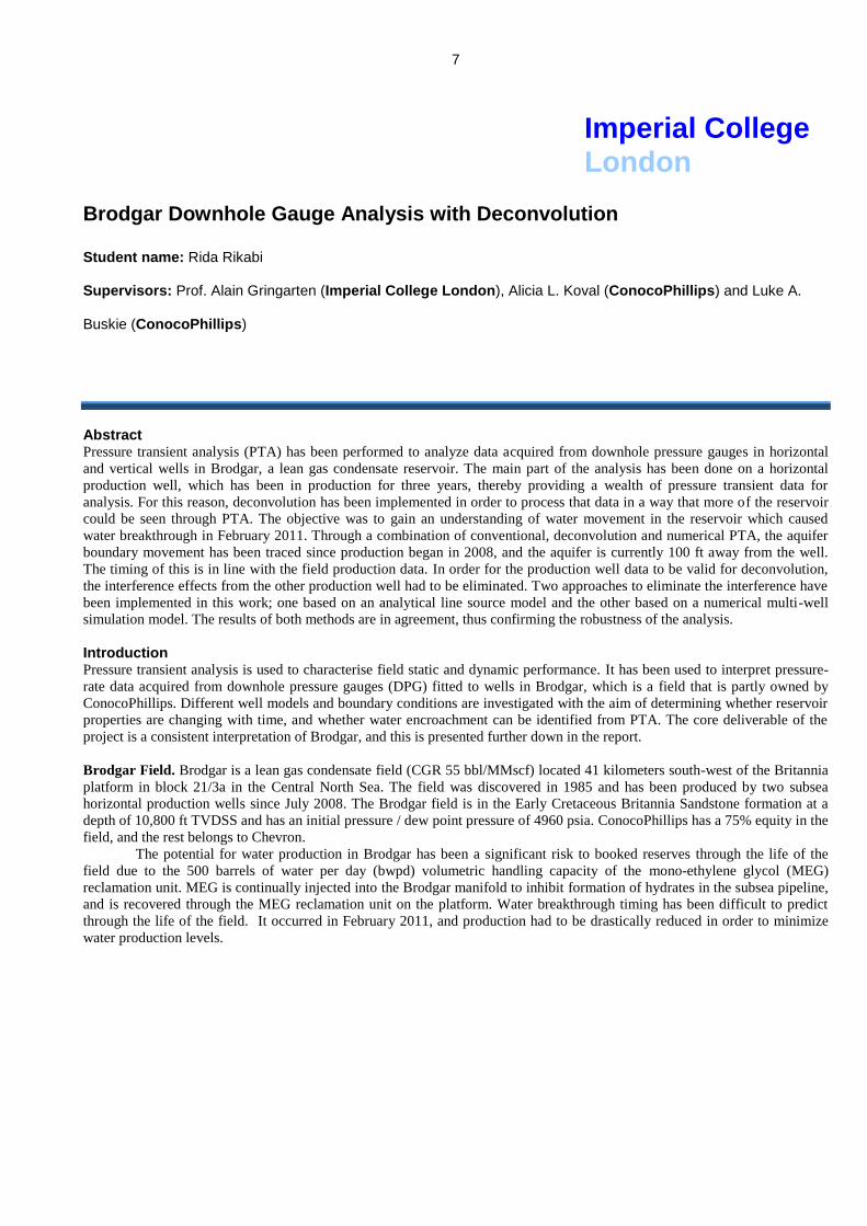
Figure 1: Plan view (top) and cross-sectional view (bottom)

of horizontal Brodgar and its wells. Top view is a contoured

depth map of the Brodgar field showing well locations and

available pressure data. Bottom view is an upscaled horizontal

permeability plot.............................................................................................................................................................................8

Figure 2: Production history of Brodgar from its two wells...........................................................................................................8

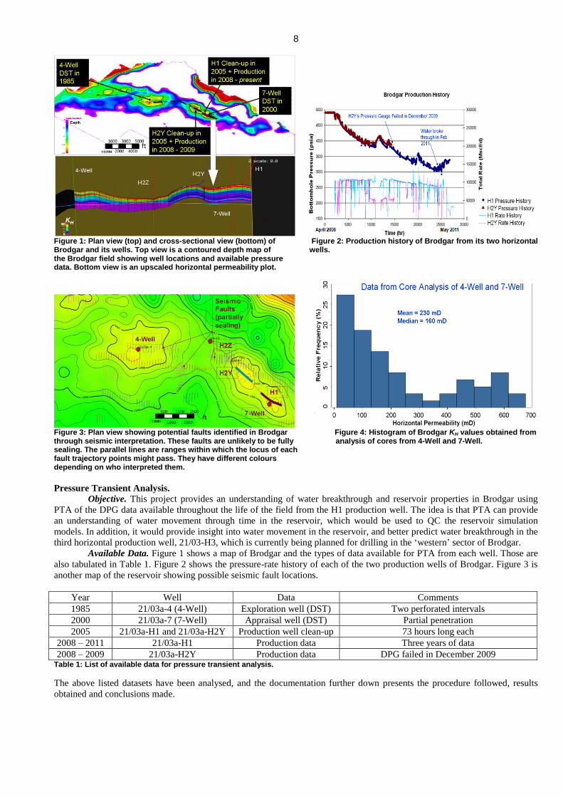
Figure 3: Plan view showing potential faults identified in Brodgar

through seismic interpretation. These faults are unlikely to be

fully sealing. The parallel lines are ranges within which the locus

of each fault trajectory points might pass. They have different

colours depending on who interpreted them...................................................................................................................................8

Figure 4: Histogram of Brodgar KH values obtained from

analysis of cores from 4-Well and 7-Well................................................................................... ....................................................8

Figure 5: BU3 model and convolved pressure data match

measured pressure data (4-Well)....................................................................................................................................................11

Figure 6: BU2 model and convolved pressure data match

measured pressure data (4-Well)..................................................................................... ...............................................................11

Figure 7: BU3 model data matches pseudo-pressure and

derivative data (4-Well).............................................................................................................. ....................................................12

Figure 8: BU3 model data matches convolved pseudo-pressure and

deconvolved derivative data (4-Well)......................................................................................... ...................................................12

Figure 9: BU2 model data matches pseudo-pressure and

derivative data (4-Well)........................................................................................................................ .........................................12

Figure 10: BU2 model data matches convolved pseudo-pressure

and deconvolved derivative data (4-Well). ...................................................................................................................................12

Figure 11: Model data matches BU4 pseudo-pressure and

derivative data (7-Well) ................................................................................................... .............................................................12

Figure 12: Model data matches BU4 convolved pseudo-pressure and

deconvolved derivative data (7-Well)............................................................................................................................................12

Figure 13: Model data matches BU1 pseudo-pressure and

derivative data (7-Well).................................................................................................................................................................13

Figure 14: Deconvolution of BU1 failed, which is evidenced by the

mismatch between convolved and measured pressure (7-Well)................................................................................... ................13

Figure 15: Model data matches convolved/deconvolved response,

which is a result of deconvolution of BU4 data combined with

BU1 late-time data (7-Well)...........................................................................................................................................................13

Figure 16: Model and convolved pressure data match measured

pressure data (7-Well)........................................................................................... .........................................................................13

Figure 17: Interpretation of Brodgar based on analysis

of the data from DSTs and clean-up periods..................................................................................................................................13

Figure 18: Model data matches build-up pseudo-pressure and

derivative data (H2Y) ...........................................................................................................................................................14

Figure 19: Model data matches build-up convolved pseudo-

pressure and deconvolved derivative data (H2Y) .........................................................................................................................14

Figure 20: Model data matches build-up pseudo-pressure and

derivative data (H1) ......................................................................................................................................................................14

Figure 21: Model data matches build-up convolved pseudo-

pressure and deconvolved derivative data (H1) .................................................................................................... .......................14

Figure 22: Model pressure data matches measured pressure data (H2Y).......................................................... ..........................14

Figure 23: Model pressure data matches measured pressure data (H1)........................................................... ............................14

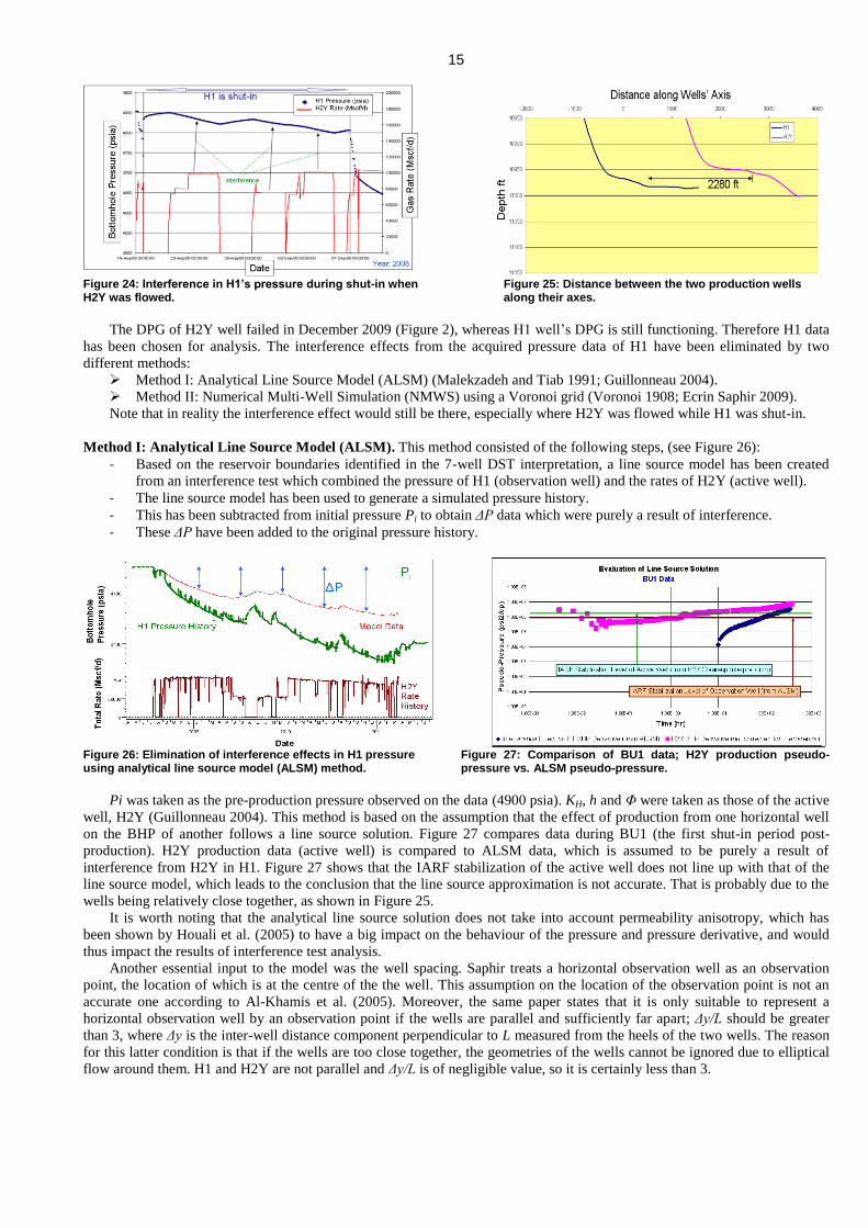
Figure 24: Interference in H1’s pressure during shut-in when

H2Y was flowed.......................................................................................................................... ...................................................15

Figure 25: Distance between the two production wells

along their axes.................................................................................................................................... ...........................................15

Figure 26: Elimination of interference effects in H1 pressure

using analytical line source model (ALSM) method.....................................................................................................................15

Figure 27: Comparison of BU1 data; H2Y production pseudo-pressure

vs. ALSM pseudo-pressure............................................................................................................................................................15

5 Figure 28: Elimination of interference effects in H1 pressure

using numerical multi-well simulation (NMWS) method..............................................................................................................16

Figure 29: Voronoi grid used for numerical simulation in order to

eliminate interference effects in H1 BHP using NMWS. The grid

includes an open rectangle boundary and both horizontal wells....................................................................................................16

Figure 30: Comparison of pressure datasets resulting from two

methods of interference removal and original pressure history.....................................................................................................16

Figure 31: Build-ups 2 – 5 overlaid (original data) .......................................................................................................................16

Figure 32: Quality check of both corrected-for-interference

datasets against 7-Well DST model (log-log) ...............................................................................................................................17

Figure 33: Quality check of both corrected-for-interference

datasets against 7-Well DST model (semi-log) ............................................................................................................................17

Figure 34: Build-ups 2 – 5 overlaid (corrected using ALSM) ......................................................................................................17

Figure 35: Build-ups 2 – 5 overlaid (corrected using NMWS) .....................................................................................................17

Figure 36: BU2 data and model (ALSM) ......................................................................................................................................18




Figure 40: BU2 data and model (NMWS) ....................................................................................................................................18

Figure 41: BU3 data and model (NMWS) ....................................................................................................................................18

Figure 42: BU4 data and model (NMWS) ................................................................................................... .................................18

Figure 43: BU5 data and model (NMWS)................................................................................................................... ..................18

Figure 44: Convolved/Deconvolved Build-ups 2 – 5 overlaid

(corrected using ALSM) ................................................................................................................................................................19

Figure 45: Convolved/Deconvolved Build-ups 2 – 5 overlaid

(corrected using NMWS) ..............................................................................................................................................................19

Figure 46: BU2 convolved/deconvolved data and model (ALSM).

Grid map is shown and dimensions are given in ft........................................................................................................................19






Grid map is shown and dimensions are given in ft.......................................................................................................................20

Figure50: BU2 convolved/deconvolved data and model (NMWS).


Figure 51: BU3 convolved/deconvolved data and model (NMWS).






Figure C-1: 4-Well Data................................................................................................................................................................33

Figure C-2: Rate history of 4-Well DST indicating stages of completion....................................................................................33

Figure D-1: 7-Well Data................................................................................................................................................................34

6 List of Tables

Table 1: List of available data for pressure transient analysis.........................................................................................................8

Table 2: Model parameters for all interpretations

of H1 production pressure build-up data

(conventional and deconvolution analyses)...................................................................................................................................13

Table B-1: PVT data used to transform pressure into gas pseudo-pressure..................................................................................32

Table E-1: Analytical line source model parameters.....................................................................................................................35

Table E-2: Numerical Multi-Well Model Parameters....................................................................................................................35

7

Brodgar Downhole Gauge Analysis with Deconvolution Student name: Rida Rikabi

Supervisors: Prof. Alain Gringarten (Imperial College London), Alicia L. Koval (ConocoPhillips) and Luke A.

Buskie (ConocoPhillips)

Abstract Pressure transient analysis (PTA) has been performed to analyze data acquired from downhole pressure gauges in horizontal

and vertical wells in Brodgar, a lean gas condensate reservoir. The main part of the analysis has been done on a horizontal

production well, which has been in production for three years, thereby providing a wealth of pressure transient data for

analysis. For this reason, deconvolution has been implemented in order to process that data in a way that more of the reservoir

could be seen through PTA. The objective was to gain an understanding of water movement in the reservoir which caused

water breakthrough in February 2011. Through a combination of conventional, deconvolution and numerical PTA, the aquifer

boundary movement has been traced since production began in 2008, and the aquifer is currently 100 ft away from the well.

The timing of this is in line with the field production data. In order for the production well data to be valid for deconvolution,

the interference effects from the other production well had to be eliminated. Two approaches to eliminate the interference have

been implemented in this work; one based on an analytical line source model and the other based on a numerical multi-well

simulation model. The results of both methods are in agreement, thus confirming the robustness of the analysis.

Introduction Pressure transient analysis is used to characterise field static and dynamic performance. It has been used to interpret pressure-

rate data acquired from downhole pressure gauges (DPG) fitted to wells in Brodgar, which is a field that is partly owned by

ConocoPhillips. Different well models and boundary conditions are investigated with the aim of determining whether reservoir

properties are changing with time, and whether water encroachment can be identified from PTA. The core deliverable of the

project is a consistent interpretation of Brodgar, and this is presented further down in the report.

Brodgar Field. Brodgar is a lean gas condensate field (CGR 55 bbl/MMscf) located 41 kilometers south-west of the Britannia

platform in block 21/3a in the Central North Sea. The field was discovered in 1985 and has been produced by two subsea

horizontal production wells since July 2008. The Brodgar field is in the Early Cretaceous Britannia Sandstone formation at a

depth of 10,800 ft TVDSS and has an initial pressure / dew point pressure of 4960 psia. ConocoPhillips has a 75% equity in the

field, and the rest belongs to Chevron.

The potential for water production in Brodgar has been a significant risk to booked reserves through the life of the

field due to the 500 barrels of water per day (bwpd) volumetric handling capacity of the mono-ethylene glycol (MEG)

reclamation unit. MEG is continually injected into the Brodgar manifold to inhibit formation of hydrates in the subsea pipeline,

and is recovered through the MEG reclamation unit on the platform. Water breakthrough timing has been difficult to predict

through the life of the field. It occurred in February 2011, and production had to be drastically reduced in order to minimize

water production levels.

Imperial College London

8

Figure 1: Plan view (top) and cross-sectional view (bottom) of Figure 2: Production history of Brodgar from its two horizontal Brodgar and its wells. Top view is a contoured depth map of wells. the Brodgar field showing well locations and available pressure data. Bottom view is an upscaled horizontal permeability plot.

Figure 3: Plan view showing potential faults identified in Brodgar Figure 4: Histogram of Brodgar KH values obtained from through seismic interpretation. These faults are unlikely to be fully analysis of cores from 4-Well and 7-Well. sealing. The parallel lines are ranges within which the locus of each fault trajectory points might pass. They have different colours depending on who interpreted them.

Pressure Transient Analysis.

Objective. This project provides an understanding of water breakthrough and reservoir properties in Brodgar using

PTA of the DPG data available throughout the life of the field from the H1 production well. The idea is that PTA can provide

an understanding of water movement through time in the reservoir, which would be used to QC the reservoir simulation

models. In addition, it would provide insight into water movement in the reservoir, and better predict water breakthrough in the

third horizontal production well, 21/03-H3, which is currently being planned for drilling in the ‘western’ sector of Brodgar.

Available Data. Figure 1 shows a map of Brodgar and the types of data available for PTA from each well. Those are

also tabulated in Table 1. Figure 2 shows the pressure-rate history of each of the two production wells of Brodgar. Figure 3 is

another map of the reservoir showing possible seismic fault locations.

Year Well Data Comments

1985 21/03a-4 (4-Well) Exploration well (DST) Two perforated intervals

2000 21/03a-7 (7-Well) Appraisal well (DST) Partial penetration

2005 21/03a-H1 and 21/03a-H2Y Production well clean-up 73 hours long each

2008 – 2011 21/03a-H1 Production data Three years of data

2008 – 2009 21/03a-H2Y Production data DPG failed in December 2009 Table 1: List of available data for pressure transient analysis.

The above listed datasets have been analysed, and the documentation further down presents the procedure followed, results

obtained and conclusions made.

9

Deconvolution. Deconvolution is a mathematical formulation used to process pressure transient data. It converts

pressure data from several flow periods with various production rates into a single unit rate drawdown. The drawdown has the

duration of the entire pressure-rate history, which means that its late-time behaviour is considerably longer than that of any of

the individual flow periods. This enables the deconvolved derivative to show boundaries to flow that are too far away to be

seen on the derivative of any individual flow period. By having a permanent DPG fitted to a production well, years of pressure

transient data could be made available for deconvolution, which would provide an increased radius of investigation.

Deconvolution is central to the analysis presented in this work, as each of the datasets listed in Table 1 has been analysed both

in the conventional manner and using deconvolution. Note that throughout this work, ‘derivative’ refers to the pressure

derivative of Bourdet et al. (1983).

Literature Review Deconvolution of pressure-rate history has been the subject of research by several authors during the last 40 years. The modern

use of deconvolution to facilitate the analysis of pressure transient data began in 2001 with the introduction of a formulation

based on the logarithm of the response function by von Schroeter et al. (2001). This formulation implemented deconvolution as

a nonlinear total least squares problem. These authors also introduced a new error model that takes into account errors in both

pressure and production rate data. These authors improved their method in von Schroeter et al. (2002) by incorporating the

variable projection algorithm, which by then was standard for minimization of the separable error measure.

Levitan (2003) evaluated von Schroeter et al.’s algorithm for application to real test data. He found that the algorithm

fails when applied to inconsistent data; which is the case for most real data, due to changing wellbore storage and rate-

dependent skin. However, he suggested using the algorithm for single flow periods (of constant rate) for interpretation. He also

suggested comparison of the deconvolved data of several flow periods in order to identify initial reservoir pressure.

Horizontal wells have seen widespread use since the early 1980s due to their high productivity in early-life (Ozkan

1999). Therefore, well test analysis has been extended to enable the interpretation of pressure transient behaviour of horizontal

wells, which is different from a vertical well’s behaviour. The main difference is the fact that a horizontal well typically sees

two flow stabilizations; radial flow in the vertical plane at early time and pseudo-radial flow in the areal (horizontal) plane at

intermediate time. This phenomenon was first expressed analytically by Daviau et al. (1985). Kuchuk et al. (1990) showed the

importance of analyzing the build-up after the first drawdown in horizontal wells, highlighting that pressure analysis without

rate measurements is insufficient for horizontal well test analysis. Kuchuk et al. (1991) introduced the analysis of horizontal

wells using the pressure derivative, where they identified the typical flow regimes. That same year, Malekzadeh and Tiab

(1991) introduced dimensionless pressure and pressure derivative type curves for interference testing of horizontal wells with

appropriate equations. Then, Ozkan (1999) gave a holistic methodology for interpreting horizontal well responses, and

highlighted the strengths and weaknesses of every approach suggested in the previous literature. He also mentioned the benefits

that a stable deconvolution algorithm could bring to the analysis of horizontal wells, which was before von Schroeter et al.

published their deconvolution algorithm mentioned above.

Research Method: Pressure Transient Analysis PTA makes use of pressure transient data to estimate certain well and reservoir properties (ex. Permeability, thickness, and

flow boundaries). This data could be obtained from a dedicated well test (ex. DST) or from data acquired from a DPG over the

producing life of the well. The results of any PTA come with a range of uncertainty on each of KH.h, KH, C, S and flow

boundary distances (Azi et al. 2008). The aim of doing PTA on Brodgar’s data was to gain an insight into the reservoir’s

properties and how they may have changed through time due to water movement in the reservoir, which eventually resulted in

water breakthrough. This is important for two reasons:

- Improving the ability to forecast production from Brodgar.

- The insights could be useful for the monitoring of the future 21/3A-H3 production well.

Although data was already available on the permeability of Brodgar, K, from core analysis (Figure 4), this was taken

on discrete core plugs, which described small sections of the reservoir, whereas an estimate from PTA would provide a better

understanding of the reservoir’s effective permeability. The uncertainty on h is quite low due to the availability of wireline log

data. However, the importance of reservoir thickness comes into play when analysing the production data because it is

important to find out if that is showing a reduction in h through time due to water encroachment, and if so by how much. As for

the flow boundaries, these could correspond either to seismic faults, sub-seismic faults (not detected due to the poor resolution

of the seismic survey) or any other form of boundary to flow. Seismic interpretations indicate the presence of faults within the

vicinity of Brodgar’s production wells, as shown in Figure 3, although they are not believed to be fully sealing. There is

uncertainty around the existence, location and degree of leakiness of these faults. Flow boundaries can also result in pressure

maintenance as opposed to depletion (which results from sealing boundaries). A constant pressure boundary could either be a

gas cap or an aquifer. If the aquifer is weak and is moving slowly however, it can act as a sealing boundary by causing apparent

depletion at its interface with the gas or oil. This is due to the rapid decrease in gas (or oil) relative permeability caused by the

decrease in saturation at the interface.

Single-Phase Gas Pseudo-Pressure. Brodgar is a lean gas condensate field, with a CGR of 55 bbl/MMscf. None of the

available pressure transient datasets exhibits composite behaviour. Therefore, it was deemed appropriate to analyse Brodgar as

10 a single-phase gas reservoir. The condensate flow rates, recorded in bbl/d, have been converted to Mscf/d and then added on to

the gas flow rates to give total gas flow rates in Mscf/d. Due to compressibility effects, the pressure transient response of a real

gas is not linear; thus it cannot be solved by analytical methods (Al-Hussainy et al. 1966). Therefore, the pressure P data is

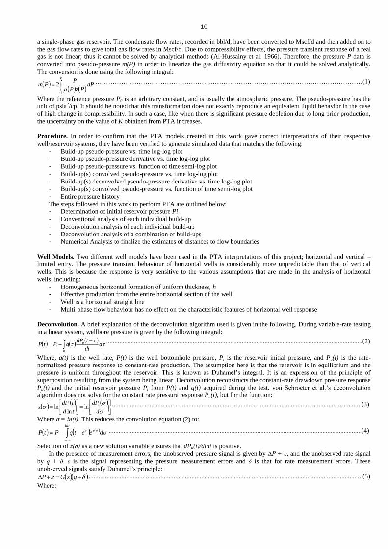
converted into pseudo-pressure m(P) in order to linearize the gas diffusivity equation so that it could be solved analytically.

The conversion is done using the following integral:

P

P

dPPzP

PPm

0

2

……………………………………………………………………………………………………………(1)

Where the reference pressure P0 is an arbitrary constant, and is usually the atmospheric pressure. The pseudo-pressure has the

unit of psia2/cp. It should be noted that this transformation does not exactly reproduce an equivalent liquid behavior in the case

of high change in compressibility. In such a case, like when there is significant pressure depletion due to long prior production,

the uncertainty on the value of K obtained from PTA increases.

Procedure. In order to confirm that the PTA models created in this work gave correct interpretations of their respective

well/reservoir systems, they have been verified to generate simulated data that matches the following:

- Build-up pseudo-pressure vs. time log-log plot

- Build-up pseudo-pressure derivative vs. time log-log plot

- Build-up pseudo-pressure vs. function of time semi-log plot

- Build-up(s) convolved pseudo-pressure vs. time log-log plot

- Build-up(s) deconvolved pseudo-pressure derivative vs. time log-log plot

- Build-up(s) convolved pseudo-pressure vs. function of time semi-log plot

- Entire pressure history

The steps followed in this work to perform PTA are outlined below:

- Determination of initial reservoir pressure Pi

- Conventional analysis of each individual build-up

- Deconvolution analysis of each individual build-up

- Deconvolution analysis of a combination of build-ups

- Numerical Analysis to finalize the estimates of distances to flow boundaries

Well Models. Two different well models have been used in the PTA interpretations of this project; horizontal and vertical –

limited entry. The pressure transient behaviour of horizontal wells is considerably more unpredictable than that of vertical

wells. This is because the response is very sensitive to the various assumptions that are made in the analysis of horizontal

wells, including:

- Homogeneous horizontal formation of uniform thickness, h

- Effective production from the entire horizontal section of the well

- Well is a horizontal straight line

- Multi-phase flow behaviour has no effect on the characteristic features of horizontal well response

Deconvolution. A brief explanation of the deconvolution algorithm used is given in the following. During variable-rate testing

in a linear system, wellbore pressure is given by the following integral:

t

ui d

dt

tdPqPtP

0

.............................................................................................................................................................(2)

Where, q(t) is the well rate, P(t) is the well bottomhole pressure, Pi is the reservoir initial pressure, and Pu(t) is the rate-

normalized pressure response to constant-rate production. The assumption here is that the reservoir is in equilibrium and the

pressure is uniform throughout the reservoir. This is known as Duhamel’s integral. It is an expression of the principle of

superposition resulting from the system being linear. Deconvolution reconstructs the constant-rate drawdown pressure response

Pu(t) and the initial reservoir pressure Pi from P(t) and q(t) acquired during the test. von Schroeter et al.’s deconvolution

algorithm does not solve for the constant rate pressure response Pu(t), but for the function:

d

dP

td

tdPz uu ln

lnln ............................................................................................................................................. ............(3)

Where σ = ln(t). This reduces the convolution equation (2) to:

t

z

i deetqPtP

ln

...........................................................................................................................................................(4)

Selection of z(σ) as a new solution variable ensures that dPu(t)/dlnt is positive.

In the presence of measurement errors, the unobserved pressure signal is given by ∆P + ε, and the unobserved rate signal

by q + δ. ε is the signal representing the pressure measurement errors and δ is that for rate measurement errors. These

unobserved signals satisfy Duhamel’s principle:

qzGP ........................................................................................................................................................................(5)

Where:

11

- z is a vector (z1,……, zn), which when multiplied by a fixed set of interpolants (ψk, k = 1,…., n) yields:

n

k

kkzz1

..............................................................................................................................................................(6)

- G(z) is the matrix of the set of equations which result from evaluating Equation (2) at times t = ti:

qzGP ......................................................................................................................................................................(7 )

The aim when implementing deconvolution is to arrive at a result in which the vectors ε and δ are small and in which the

response z is sufficiently smooth. The algorithm achieves that through the minimization of the term, E, given below: 2

2

2

2

2

2kDzE .............................................................................................................................................................(8)

Where ν is a weight factor which takes into account the rate match and the pressure match, and λ is the weight factor which

accounts for curvature (smoothness). The user manipulates these two parameters until he/she arrives at a deconvolved

derivative which is not too noisy (i.e. too many curves), yet preserves the genuine features of the reservoir indicated on the

Bourdet derivative. On KAPPA’s Saphir PTA software, which has been used throughout this work, these two variables are

related to other input parameters1; λ is related to ‘smoothing’, and ν is related to ‘rate relative weight’ and ‘pressure relative

weight’. Different values of smoothing have been used for different interpretations in this work, but for all analyses ‘rate

relative weight’ = 1 and ‘pressure relative weight’ = 10. xxx T2

denotes the 2-norm of a vector, x. D and k are a constant

matrix and vector, respectively, chosen such that 2

kDz is a measure of the smoothness of z. Thereby ε, δ and z are estimated

based on the choice of ν and λ.

Full details of the deconvolution algorithm used in this work can be found in von Schroeter et al. (2001), von Schroeter et

al. (2002) and Levitan (2003).

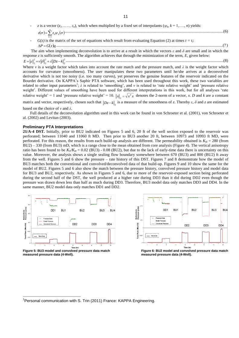
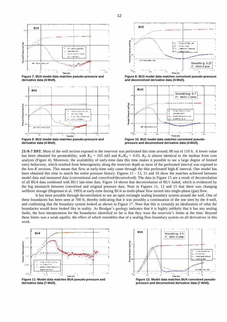
Preliminary PTA Interpretations 21/A-4 DST. Initially, prior to BU2 indicated on Figures 5 and 6, 20 ft of the well section exposed to the reservoir was

perforated; between 11040 and 11060 ft MD. Then prior to BU3 another 20 ft, between 10973 and 10993 ft MD, were

perforated. For this reason, the results from each build-up analysis are different. The permeability obtained is KH = 280 (from

BU2) – 330 (from BU3) mD, which is a range close to the mean obtained from core analysis (Figure 4). The vertical anisotropy

ratio has been found to be KV/KH = 0.02 (BU3) - 0.08 (BU2), but due to the lack of early-time data there is uncertainty on this

value. Moreover, the analysis shows a single sealing flow boundary somewhere between 670 (BU3) and 800 (BU2) ft away

from the well. Figures 5 and 6 show the pressure – rate history of this DST. Figures 7 and 8 demonstrate how the model of

BU3 matches both the conventional and convolved/deconvolved data of that build-up. Figures 9 and 10 show the same for the

model of BU2. Figures 5 and 6 also show the match between the pressure history, convolved pressure history and model data

for BU3 and BU2, respectively. As shown in Figures 5 and 6, due to more of the reservoir-exposed section being perforated

during the second half of the DST, the well produced at a higher rate during DD3 than it did during DD2 even though the

pressure was drawn down less than half as much during DD3. Therefore, BU3 model data only matches DD3 and DD4. In the

same manner, BU2 model data only matches DD1 and DD2.

Figure 5: BU3 model and convolved pressure data match Figure 6: BU2 model and convolved pressure data match measured pressure data (4-Well). measured pressure data (4-Well).

1Personal communication with S. Trin (2011) France: KAPPA Engineering.

12

Figure 7: BU3 model data matches pseudo-pressure and Figure 8: BU3 model data matches convolved pseudo-pressure derivative data (4-Well). and deconvolved derivative data (4-Well).

Figure 9: BU2 model data matches pseudo-pressure and Figure 10: BU2 model data matches convolved pseudo- derivative data (4-Well). pressure and deconvolved derivative data (4-Well).

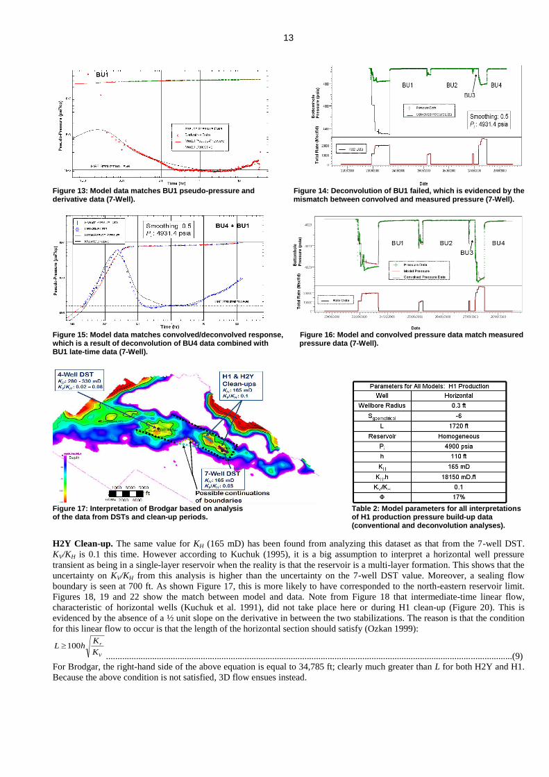
21/A-7 DST. Most of the well section exposed to the reservoir was perforated this time around; 88 out of 110 ft. A lower value

has been obtained for permeability, with KH = 165 mD and KV/KH = 0.03. KH is almost identical to the median from core

analysis (Figure 4). Moreover, the availability of early-time data this time makes it possible to see a large degree of limited

entry behaviour, which resulted from heterogeneity along the reservoir depth as most of the perforated interval was exposed to

the low-K sections. This meant that flow at early-time only came through the thin perforated high-K interval. One model has

been obtained this time to match the entire pressure history. Figures 11 - 13, 15 and 16 show the matches achieved between

model data and measured data (conventional and convolved/deconvolved). The data in Figure 15 are a result of deconvolution

of all BU4 data combined with BU1 late-time data. Figure 14 shows that deconvolution of BU1 failed, which is evidenced by

the big mismatch between convolved and original pressure data. Note in Figures 11, 12 and 15 that there was changing

wellbore storage (Hegeman et al. 1993) at early-time during BU4 as multi-phase flow turned into single-phase (gas) flow.

It has been possible through deconvolution to see an open rectangle sealing boundary system around the well. One of

these boundaries has been seen at 700 ft, thereby indicating that it was possibly a continuation of the one seen by the 4-well,

and confirming that the boundary system looked as shown in Figure 17. Note that this is certainly an idealization of what the

boundaries would have looked like in reality. As Brodgar’s geology indicates that it is highly unlikely that it has any sealing

faults, the best interpretation for the boundaries identified so far is that they were the reservoir’s limits at the time. Beyond

these limits was a weak aquifer, the effect of which resembles that of a sealing flow boundary system on all derivatives in this

work.

Figure 11: Model data matches BU4 pseudo-pressure and Figure 12: Model data matches BU4 convolved pseudo- derivative data (7-Well). pressure and deconvolved derivative data (7-Well).

13

Figure 13: Model data matches BU1 pseudo-pressure and Figure 14: Deconvolution of BU1 failed, which is evidenced by the derivative data (7-Well). mismatch between convolved and measured pressure (7-Well).

Figure 15: Model data matches convolved/deconvolved response, Figure 16: Model and convolved pressure data match measured which is a result of deconvolution of BU4 data combined with pressure data (7-Well). BU1 late-time data (7-Well).

Figure 17: Interpretation of Brodgar based on analysis Table 2: Model parameters for all interpretations of the data from DSTs and clean-up periods. of H1 production pressure build-up data

(conventional and deconvolution analyses).

H2Y Clean-up. The same value for KH (165 mD) has been found from analyzing this dataset as that from the 7-well DST.

KV/KH is 0.1 this time. However according to Kuchuk (1995), it is a big assumption to interpret a horizontal well pressure

transient as being in a single-layer reservoir when the reality is that the reservoir is a multi-layer formation. This shows that the

uncertainty on KV/KH from this analysis is higher than the uncertainty on the 7-well DST value. Moreover, a sealing flow

boundary is seen at 700 ft. As shown Figure 17, this is more likely to have corresponded to the north-eastern reservoir limit.

Figures 18, 19 and 22 show the match between model and data. Note from Figure 18 that intermediate-time linear flow,

characteristic of horizontal wells (Kuchuk et al. 1991), did not take place here or during H1 clean-up (Figure 20). This is

evidenced by the absence of a ½ unit slope on the derivative in between the two stabilizations. The reason is that the condition

for this linear flow to occur is that the length of the horizontal section should satisfy (Ozkan 1999):

V

r

K

KhL 100

................................................................................................................................................................................(9)

For Brodgar, the right-hand side of the above equation is equal to 34,785 ft; clearly much greater than L for both H2Y and H1.

Because the above condition is not satisfied, 3D flow ensues instead.

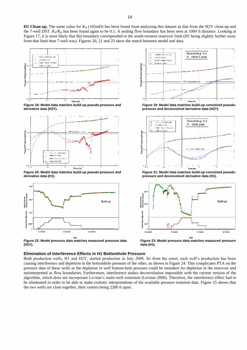
14 H1 Clean-up. The same value for KH (165mD) has been found from analyzing this dataset as that from the H2Y clean-up and

the 7-well DST. KV/KH has been found again to be 0.1. A sealing flow boundary has been seen at 1000 ft distance. Looking at

Figure 17, it is most likely that this boundary corresponded to the south-western reservoir limit (H1 being slightly further away

from that limit than 7-well was). Figures 20, 21 and 23 show the match between model and data.

Figure 18: Model data matches build-up pseudo-pressure and Figure 19: Model data matches build-up convolved pseudo- derivative data (H2Y). pressure and deconvolved derivative data (H2Y).

Figure 20: Model data matches build-up pseudo-pressure and Figure 21: Model data matches build-up convolved pseudo- derivative data (H1). pressure and deconvolved derivative data (H1).

Figure 22: Model pressure data matches measured pressure data Figure 23: Model pressure data matches measured pressure (H2Y). data (H1).

Elimination of Interference Effects in H1 Bottomhole Pressure

Both production wells, H1 and H2Y, started production in July 2008. So from the onset, each well’s production has been

causing interference and depletion in the bottomhole pressure of the other, as shown in Figure 24. This complicates PTA on the

pressure data of these wells as the depletion in well bottom-hole pressure could be mistaken for depletion in the reservoir and

misinterpreted as flow boundaries. Furthermore, interference makes deconvolution impossible with the current version of the

algorithm, which does not incorporate Levitan’s multi-well extension (Levitan 2006). Therefore, the interference effect had to

be eliminated in order to be able to make realistic interpretations of the available pressure transient data. Figure 25 shows that

the two wells are close together, their centres being 2280 ft apart.

15

Figure 24: Interference in H1’s pressure during shut-in when Figure 25: Distance between the two production wells H2Y was flowed. along their axes.

The DPG of H2Y well failed in December 2009 (Figure 2), whereas H1 well’s DPG is still functioning. Therefore H1 data

has been chosen for analysis. The interference effects from the acquired pressure data of H1 have been eliminated by two

different methods:

Method I: Analytical Line Source Model (ALSM) (Malekzadeh and Tiab 1991; Guillonneau 2004).

Method II: Numerical Multi-Well Simulation (NMWS) using a Voronoi grid (Voronoi 1908; Ecrin Saphir 2009).

Note that in reality the interference effect would still be there, especially where H2Y was flowed while H1 was shut-in.

Method I: Analytical Line Source Model (ALSM). This method consisted of the following steps, (see Figure 26):

- Based on the reservoir boundaries identified in the 7-well DST interpretation, a line source model has been created

from an interference test which combined the pressure of H1 (observation well) and the rates of H2Y (active well).

- The line source model has been used to generate a simulated pressure history.

- This has been subtracted from initial pressure Pi to obtain ΔP data which were purely a result of interference.

- These ΔP have been added to the original pressure history.

Figure 26: Elimination of interference effects in H1 pressure Figure 27: Comparison of BU1 data; H2Y production pseudo- using analytical line source model (ALSM) method. pressure vs. ALSM pseudo-pressure.

Pi was taken as the pre-production pressure observed on the data (4900 psia). KH, h and Φ were taken as those of the active

well, H2Y (Guillonneau 2004). This method is based on the assumption that the effect of production from one horizontal well

on the BHP of another follows a line source solution. Figure 27 compares data during BU1 (the first shut-in period post-

production). H2Y production data (active well) is compared to ALSM data, which is assumed to be purely a result of

interference from H2Y in H1. Figure 27 shows that the IARF stabilization of the active well does not line up with that of the

line source model, which leads to the conclusion that the line source approximation is not accurate. That is probably due to the

wells being relatively close together, as shown in Figure 25.

It is worth noting that the analytical line source solution does not take into account permeability anisotropy, which has

been shown by Houali et al. (2005) to have a big impact on the behaviour of the pressure and pressure derivative, and would

thus impact the results of interference test analysis.

Another essential input to the model was the well spacing. Saphir treats a horizontal observation well as an observation

point, the location of which is at the centre of the the well. This assumption on the location of the observation point is not an

accurate one according to Al-Khamis et al. (2005). Moreover, the same paper states that it is only suitable to represent a

horizontal observation well by an observation point if the wells are parallel and sufficiently far apart; Δy/L should be greater

than 3, where Δy is the inter-well distance component perpendicular to L measured from the heels of the two wells. The reason

for this latter condition is that if the wells are too close together, the geometries of the wells cannot be ignored due to elliptical

flow around them. H1 and H2Y are not parallel and Δy/L is of negligible value, so it is certainly less than 3.

16

Based on the above discussion, there are four contributors to the uncertainty around the results of the ALSM method. The

effects of these factors will be shown to be non-negligible further down in the text.

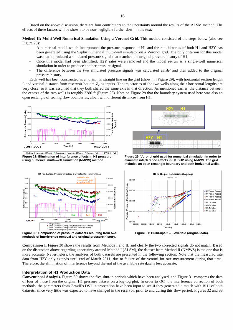
Method II: Multi-Well Numerical Simulation Using a Voronoi Grid. This method consisted of the steps below (also see

Figure 28):

- A numerical model which incorporated the pressure response of H1 and the rate histories of both H1 and H2Y has

been generated using the Saphir numerical multi-well simulator on a Voronoi grid. The only criterion for this model

was that it produced a simulated pressure signal that matched the original pressure history of H1.

- Once this model had been identified, H2Y rates were removed and the model re-run as a single-well numerical

simulation in order to produce another pressure signal.

- The difference between the two simulated pressure signals was calculated as ΔP and then added to the original

pressure history.

Each well has been constructed as a horizontal straight line on the grid (shown in Figure 29), with horizontal section length

L and vertical distance from reservoir bottom Zw as inputs. The trajectories of the two wells along their horizontal lengths are

very close, so it was assumed that they both shared the same axis in that direction. As mentioned earlier, the distance between

the centres of the two wells is roughly 2280 ft (Figure 25). Note on Figure 29 that the boundary system used here was also an

open rectangle of sealing flow boundaries, albeit with different distances from H1.

Figure 28: Elimination of interference effects in H1 pressure Figure 29: Voronoi grid used for numerical simulation in order to using numerical multi-well simulation (NMWS) method. eliminate interference effects in H1 BHP using NMWS. The grid

includes an open rectangle boundary and both horizontal wells.

Figure 30: Comparison of pressure datasets resulting from two Figure 31: Build-ups 2 – 5 overlaid (original data). methods of interference removal and original pressure history.

Comparison I. Figure 30 shows the results from Methods I and II, and clearly the two corrected signals do not match. Based

on the discussion above regarding uncertainty around Method I (ALSM), the dataset from Method II (NMWS) is the one that is

more accurate. Nevertheless, the analyses of both datasets are presented in the following section. Note that the measured rate

data from H2Y only extends until end of March 2011, due to failure of the venturi for rate measurement during that time.

Therefore, the elimination of interference beyond the end of the available rate data is less accurate.

Interpretation of H1 Production Data Conventional Analysis. Figure 30 shows the five shut-in periods which have been analysed, and Figure 31 compares the data

of four of those from the original H1 pressure dataset on a log-log plot. In order to QC the interference correction of both

methods, the parameters from 7-well’s DST interpretation have been input to see if they generated a match with BU1 of both

datasets, since very little was expected to have changed in the reservoir prior to and during this flow period. Figures 32 and 33

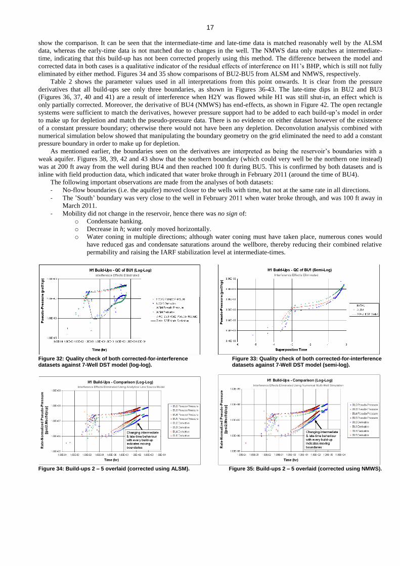
17 show the comparison. It can be seen that the intermediate-time and late-time data is matched reasonably well by the ALSM

data, whereas the early-time data is not matched due to changes in the well. The NMWS data only matches at intermediate-

time, indicating that this build-up has not been corrected properly using this method. The difference between the model and

corrected data in both cases is a qualitative indicator of the residual effects of interference on H1’s BHP, which is still not fully

eliminated by either method. Figures 34 and 35 show comparisons of BU2-BU5 from ALSM and NMWS, respectively.

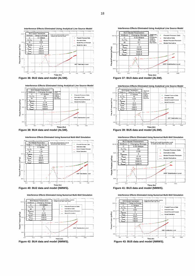
Table 2 shows the parameter values used in all interpretations from this point onwards. It is clear from the pressure

derivatives that all build-ups see only three boundaries, as shown in Figures 36-43. The late-time dips in BU2 and BU3

(Figures 36, 37, 40 and 41) are a result of interference when H2Y was flowed while H1 was still shut-in, an effect which is

only partially corrected. Moreover, the derivative of BU4 (NMWS) has end-effects, as shown in Figure 42. The open rectangle

systems were sufficient to match the derivatives, however pressure support had to be added to each build-up’s model in order

to make up for depletion and match the pseudo-pressure data. There is no evidence on either dataset however of the existence

of a constant pressure boundary; otherwise there would not have been any depletion. Deconvolution analysis combined with

numerical simulation below showed that manipulating the boundary geometry on the grid eliminated the need to add a constant

pressure boundary in order to make up for depletion.

As mentioned earlier, the boundaries seen on the derivatives are interpreted as being the reservoir’s boundaries with a

weak aquifer. Figures 38, 39, 42 and 43 show that the southern boundary (which could very well be the northern one instead)

was at 200 ft away from the well during BU4 and then reached 100 ft during BU5. This is confirmed by both datasets and is

inline with field production data, which indicated that water broke through in February 2011 (around the time of BU4).

The following important observations are made from the analyses of both datasets:

- No-flow boundaries (i.e. the aquifer) moved closer to the wells with time, but not at the same rate in all directions.

- The ’South’ boundary was very close to the well in February 2011 when water broke through, and was 100 ft away in

March 2011.

- Mobility did not change in the reservoir, hence there was no sign of:

o Condensate banking.

o Decrease in h; water only moved horizontally.

o Water coning in multiple directions; although water coning must have taken place, numerous cones would

have reduced gas and condensate saturations around the wellbore, thereby reducing their combined relative

permability and raising the IARF stabilization level at intermediate-times.

Figure 32: Quality check of both corrected-for-interference Figure 33: Quality check of both corrected-for-interference datasets against 7-Well DST model (log-log). datasets against 7-Well DST model (semi-log).

Figure 34: Build-ups 2 – 5 overlaid (corrected using ALSM). Figure 35: Build-ups 2 – 5 overlaid (corrected using NMWS).

18

Figure 36: BU2 data and model (ALSM). Figure 37: BU3 data and model (ALSM).

Figure 38: BU4 data and model (ALSM). Figure 39: BU5 data and model (ALSM).

Figure 40: BU2 data and model (NMWS). Figure 41: BU3 data and model (NMWS).

Figure 42: BU4 data and model (NMWS). Figure 43: BU5 data and model (NMWS).

Interference Effects Eliminated Using Numerical Multi-Well Simulation Interference Effects Eliminated Using Numerical Multi-Well Simulation

Interference Effects Eliminated Using Numerical Multi-Well Simulation Interference Effects Eliminated Using Numerical Multi-Well Simulation

Interference Effects Eliminated Using Analytical Line Source ModelInterference Effects Eliminated Using Analytical Line Source Model

Interference Effects Eliminated Using Analytical Line Source Model Interference Effects Eliminated Using Analytical Line Source Model

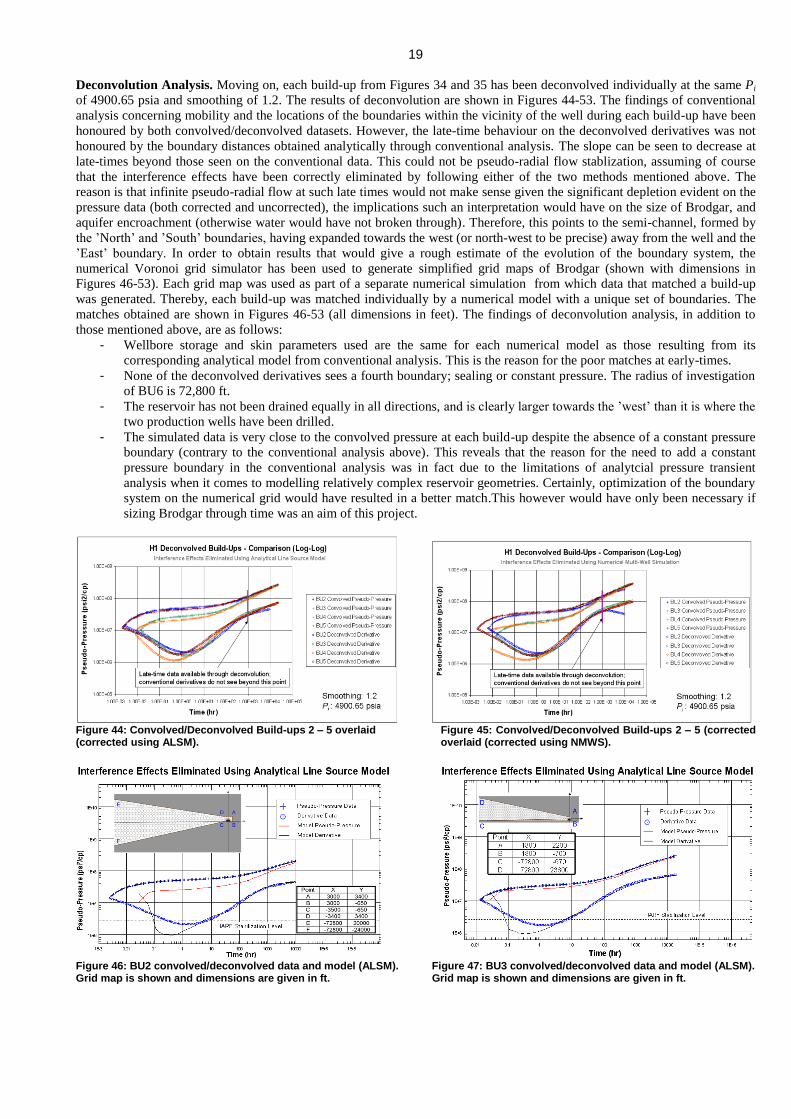
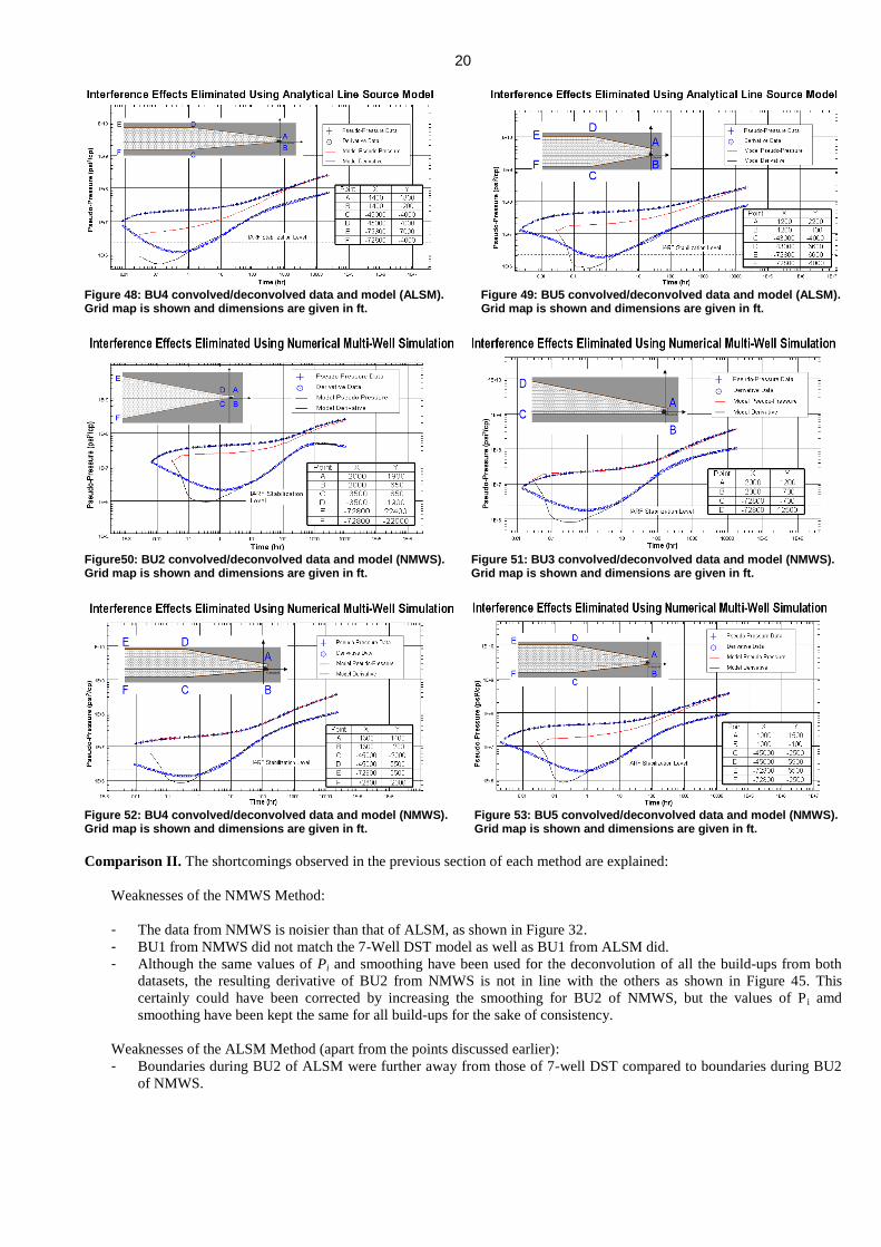
19 Deconvolution Analysis. Moving on, each build-up from Figures 34 and 35 has been deconvolved individually at the same Pi

of 4900.65 psia and smoothing of 1.2. The results of deconvolution are shown in Figures 44-53. The findings of conventional

analysis concerning mobility and the locations of the boundaries within the vicinity of the well during each build-up have been

honoured by both convolved/deconvolved datasets. However, the late-time behaviour on the deconvolved derivatives was not

honoured by the boundary distances obtained analytically through conventional analysis. The slope can be seen to decrease at

late-times beyond those seen on the conventional data. This could not be pseudo-radial flow stablization, assuming of course

that the interference effects have been correctly eliminated by following either of the two methods mentioned above. The

reason is that infinite pseudo-radial flow at such late times would not make sense given the significant depletion evident on the

pressure data (both corrected and uncorrected), the implications such an interpretation would have on the size of Brodgar, and

aquifer encroachment (otherwise water would have not broken through). Therefore, this points to the semi-channel, formed by

the ’North’ and ’South’ boundaries, having expanded towards the west (or north-west to be precise) away from the well and the

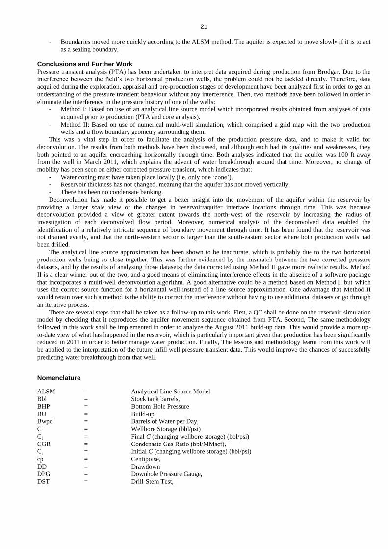
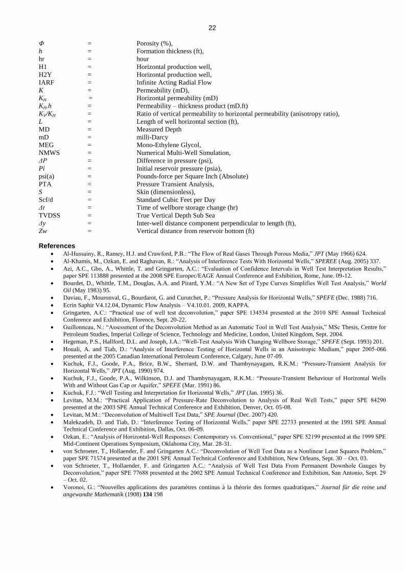
’East’ boundary. In order to obtain results that would give a rough estimate of the evolution of the boundary system, the

numerical Voronoi grid simulator has been used to generate simplified grid maps of Brodgar (shown with dimensions in

Figures 46-53). Each grid map was used as part of a separate numerical simulation from which data that matched a build-up

was generated. Thereby, each build-up was matched individually by a numerical model with a unique set of boundaries. The

matches obtained are shown in Figures 46-53 (all dimensions in feet). The findings of deconvolution analysis, in addition to

those mentioned above, are as follows:

- Wellbore storage and skin parameters used are the same for each numerical model as those resulting from its

corresponding analytical model from conventional analysis. This is the reason for the poor matches at early-times.

- None of the deconvolved derivatives sees a fourth boundary; sealing or constant pressure. The radius of investigation

of BU6 is 72,800 ft.

- The reservoir has not been drained equally in all directions, and is clearly larger towards the ’west’ than it is where the

two production wells have been drilled.

- The simulated data is very close to the convolved pressure at each build-up despite the absence of a constant pressure

boundary (contrary to the conventional analysis above). This reveals that the reason for the need to add a constant

pressure boundary in the conventional analysis was in fact due to the limitations of analytcial pressure transient

analysis when it comes to modelling relatively complex reservoir geometries. Certainly, optimization of the boundary

system on the numerical grid would have resulted in a better match.This however would have only been necessary if

sizing Brodgar through time was an aim of this project.

Figure 44: Convolved/Deconvolved Build-ups 2 – 5 overlaid Figure 45: Convolved/Deconvolved Build-ups 2 – 5 (corrected (corrected using ALSM). overlaid (corrected using NMWS).

Figure 46: BU2 convolved/deconvolved data and model (ALSM). Figure 47: BU3 convolved/deconvolved data and model (ALSM). Grid map is shown and dimensions are given in ft. Grid map is shown and dimensions are given in ft.

20

Figure 48: BU4 convolved/deconvolved data and model (ALSM). Figure 49: BU5 convolved/deconvolved data and model (ALSM). Grid map is shown and dimensions are given in ft. Grid map is shown and dimensions are given in ft.

Figure50: BU2 convolved/deconvolved data and model (NMWS). Figure 51: BU3 convolved/deconvolved data and model (NMWS). Grid map is shown and dimensions are given in ft. Grid map is shown and dimensions are given in ft.

Figure 52: BU4 convolved/deconvolved data and model (NMWS). Figure 53: BU5 convolved/deconvolved data and model (NMWS). Grid map is shown and dimensions are given in ft. Grid map is shown and dimensions are given in ft.

Comparison II. The shortcomings observed in the previous section of each method are explained:

Weaknesses of the NMWS Method:

- The data from NMWS is noisier than that of ALSM, as shown in Figure 32.

- BU1 from NMWS did not match the 7-Well DST model as well as BU1 from ALSM did.

- Although the same values of Pi and smoothing have been used for the deconvolution of all the build-ups from both

datasets, the resulting derivative of BU2 from NMWS is not in line with the others as shown in Figure 45. This

certainly could have been corrected by increasing the smoothing for BU2 of NMWS, but the values of P i amd

smoothing have been kept the same for all build-ups for the sake of consistency.

Weaknesses of the ALSM Method (apart from the points discussed earlier):

- Boundaries during BU2 of ALSM were further away from those of 7-well DST compared to boundaries during BU2

of NMWS.

21

- Boundaries moved more quickly according to the ALSM method. The aquifer is expected to move slowly if it is to act

as a sealing boundary.

Conclusions and Further Work Pressure transient analysis (PTA) has been undertaken to interpret data acquired during production from Brodgar. Due to the

interference between the field’s two horizontal production wells, the problem could not be tackled directly. Therefore, data

acquired during the exploration, appraisal and pre-production stages of development have been analyzed first in order to get an

understanding of the pressure transient behaviour without any interference. Then, two methods have been followed in order to

eliminate the interference in the pressure history of one of the wells:

- Method I: Based on use of an analytical line source model which incorporated results obtained from analyses of data

acquired prior to production (PTA and core analysis).

- Method II: Based on use of numerical multi-well simulation, which comprised a grid map with the two production

wells and a flow boundary geometry surrounding them.

This was a vital step in order to facilitate the analysis of the production pressure data, and to make it valid for

deconvolution. The results from both methods have been discussed, and although each had its qualities and weaknesses, they

both pointed to an aquifer encroaching horizontally through time. Both analyses indicated that the aquifer was 100 ft away

from the well in March 2011, which explains the advent of water breakthrough around that time. Moreover, no change of

mobility has been seen on either corrected pressure transient, which indicates that:

- Water coning must have taken place locally (i.e. only one ‘cone’).

- Reservoir thickness has not changed, meaning that the aquifer has not moved vertically.

- There has been no condensate banking.

Deconvolution has made it possible to get a better insight into the movement of the aquifer within the reservoir by

providing a larger scale view of the changes in reservoir/aquifer interface locations through time. This was because

deconvolution provided a view of greater extent towards the north-west of the reservoir by increasing the radius of

investigation of each deconvolved flow period. Moreover, numerical analysis of the deconvolved data enabled the

identification of a relatively intricate sequence of boundary movement through time. It has been found that the reservoir was

not drained evenly, and that the north-western sector is larger than the south-eastern sector where both production wells had

been drilled.

The analytical line source approximation has been shown to be inaccurate, which is probably due to the two horizontal

production wells being so close together. This was further evidenced by the mismatch between the two corrected pressure

datasets, and by the results of analysing those datasets; the data corrected using Method II gave more realistic results. Method

II is a clear winner out of the two, and a good means of eliminating interference effects in the absence of a software package

that incorporates a multi-well deconvolution algorithm. A good alternative could be a method based on Method I, but which

uses the correct source function for a horizontal well instead of a line source approximation. One advantage that Method II

would retain over such a method is the ability to correct the interference without having to use additional datasets or go through

an iterative process.

There are several steps that shall be taken as a follow-up to this work. First, a QC shall be done on the reservoir simulation

model by checking that it reproduces the aquifer movement sequence obtained from PTA. Second, The same methodology

followed in this work shall be implemented in order to analyze the August 2011 build-up data. This would provide a more up-

to-date view of what has happened in the reservoir, which is particularly important given that production has been significantly

reduced in 2011 in order to better manage water production. Finally, The lessons and methodology learnt from this work will

be applied to the interpretation of the future infill well pressure transient data. This would improve the chances of successfully

predicting water breakthrough from that well.

Nomenclature

ALSM = Analytical Line Source Model,

Bbl = Stock tank barrels,

BHP = Bottom-Hole Pressure

BU = Build-up,

Bwpd = Barrels of Water per Day,

C = Wellbore Storage (bbl/psi)

Cf = Final C (changing wellbore storage) (bbl/psi)

CGR = Condensate Gas Ratio (bbl/MMscf),

Ci = Initial C (changing wellbore storage) (bbl/psi)

cp = Centipoise,

DD = Drawdown

DPG = Downhole Pressure Gauge,

DST = Drill-Stem Test,

22 Φ = Porosity (%),

h = Formation thickness (ft),

hr = hour

H1 = Horizontal production well,

H2Y = Horizontal production well,

IARF = Infinite Acting Radial Flow

K = Permeability (mD),

KH = Horizontal permeability (mD)

KH.h = Permeability – thickness product (mD.ft)

KV/KH = Ratio of vertical permeability to horizontal permeability (anisotropy ratio),

L = Length of well horizontal section (ft),

MD = Measured Depth

mD = milli-Darcy

MEG = Mono-Ethylene Glycol,

NMWS = Numerical Multi-Well Simulation,

ΔP = Difference in pressure (psi),

Pi = Initial reservoir pressure (psia),

psi(a) = Pounds-force per Square Inch (Absolute)

PTA = Pressure Transient Analysis,

S = Skin (dimensionless),

Scf/d = Standard Cubic Feet per Day

Δt = Time of wellbore storage change (hr)

TVDSS = True Vertical Depth Sub Sea

Δy = Inter-well distance component perpendicular to length (ft),

Zw = Vertical distance from reservoir bottom (ft)

References Al-Hussainy, R., Ramey, H.J. and Crawford, P.B.: “The Flow of Real Gases Through Porous Media,” JPT (May 1966) 624.

Al-Khamis, M., Ozkan, E. and Raghavan, R.: “Analysis of Interference Tests With Horizontal Wells,” SPEREE (Aug. 2005) 337.

Azi, A.C., Gbo, A., Whittle, T. and Gringarten, A.C.: “Evaluation of Confidence Intervals in Well Test Interpretation Results,”

paper SPE 113888 presented at the 2008 SPE Europec/EAGE Annual Conference and Exhibition, Rome, June. 09-12.

Bourdet, D., Whittle, T.M., Douglas, A.A. and Pirard, Y.M.: “A New Set of Type Curves Simplifies Well Test Analysis,” World

Oil (May 1983) 95.

Daviau, F., Mouronval, G., Bourdarot, G. and Curutchet, P.: “Pressure Analysis for Horizontal Wells,” SPEFE (Dec. 1988) 716.

Ecrin Saphir V4.12.04, Dynamic Flow Analysis – V4.10.01. 2009, KAPPA.

Gringarten, A.C.: “Practical use of well test deconvolution,” paper SPE 134534 presented at the 2010 SPE Annual Technical

Conference and Exhibition, Florence, Sept. 20-22.

Guillonneau, N.: “Assessment of the Deconvolution Method as an Automatic Tool in Well Test Analysis,” MSc Thesis, Centre for

Petroleum Studies, Imperial College of Science, Technology and Medicine, London, United Kingdom, Sept. 2004.

Hegeman, P.S., Hallford, D.L. and Joseph, J.A.: “Well-Test Analysis With Changing Wellbore Storage,” SPEFE (Sept. 1993) 201.

Houali, A. and Tiab, D.: “Analysis of Interference Testing of Horizontal Wells in an Anisotropic Medium,” paper 2005-066

presented at the 2005 Canadian International Petroleum Conference, Calgary, June 07-09.

Kuchuk, F.J., Goode, P.A., Brice, B.W., Sherrard, D.W. and Thambynayagam, R.K.M.: “Pressure-Transient Analysis for

Horizontal Wells,” JPT (Aug. 1990) 974.

Kuchuk, F.J., Goode, P.A., Wilkinson, D.J. and Thambynayagam, R.K.M.: “Pressure-Transient Behaviour of Horizontal Wells

With and Without Gas Cap or Aquifer,” SPEFE (Mar. 1991) 86.

Kuchuk, F.J.: “Well Testing and Interpretation for Horizontal Wells,” JPT (Jan. 1995) 36.

Levitan, M.M.: “Practical Application of Pressure-Rate Deconvolution to Analysis of Real Well Tests,” paper SPE 84290

presented at the 2003 SPE Annual Technical Conference and Exhibition, Denver, Oct. 05-08.

Levitan, M.M.: “Deconvolution of Multiwell Test Data,” SPE Journal (Dec. 2007) 420.

Malekzadeh, D. and Tiab, D.: “Interference Testing of Horizontal Wells,” paper SPE 22733 presented at the 1991 SPE Annual

Technical Conference and Exhibition, Dallas, Oct. 06-09.

Ozkan, E.: “Analysis of Horizontal-Well Responses: Contemporary vs. Conventional,” paper SPE 52199 presented at the 1999 SPE

Mid-Continent Operations Symposium, Oklahoma City, Mar. 28-31.

von Schroeter, T., Hollaender, F. and Gringarten A.C.: “Deconvolution of Well Test Data as a Nonlinear Least Squares Problem,”

paper SPE 71574 presented at the 2001 SPE Annual Technical Conference and Exhibition, New Orleans, Sept. 30 – Oct. 03.

von Schroeter, T., Hollaender, F. and Gringarten A.C.: “Analysis of Well Test Data From Permanent Downhole Gauges by

Deconvolution,” paper SPE 77688 presented at the 2002 SPE Annual Technical Conference and Exhibition, San Antonio, Sept. 29

– Oct. 02.

Voronoi, G.: “Nouvelles applications des paramètres continus à la théorie des formes quadratiques,” Journal für die reine und

angewandte Mathematik (1908) 134 198

23

APPENDIX A: Critical Literature Review

MILESTONES IN DECONVOLUTION AND GAS CONDENSATE PRESSURE TRANSIENT ANALYSIS

TABLE OF CONTENTS

Deconvolution for Pressure Transient Analysis

SPE

Paper n

Year Title Authors Contribution

71574

2001

“Deconvolution of Well Test

Data as a Nonlinear Total

Least Squares Problem”

T. von Schroeter,

F. Hollaender, A.

C. Gringarten

These authors introduced a new method

that reformulated deconvolution as a

nonlinear Total Least Squares problem.

77688

2002

“Analysis of Well Test Data

From Permanent Downhole

Gauges by Deconvolution”

T. von Schroeter,

F. Hollaender, A.

C. Gringarten

Reported a number of improvements to

the algorithm of SPE 71574, and derived

error bounds for rate and response

estimates in the presence of uncertainties

in the data, for which the authors

assumed simple Gaussian models.

84290

2003

“Practical Application of

Pressure-Rate Deconvolution

to Analysis of Real Well

Tests”

M. M. Levitan

Independent evaluation of the algorithm

developed in SPE 71574 and 77688,

which found that it works well on

consistent sets of data. The author also

proposed enhancements of the algorithm

that allow it to be used reliably with real

test data.

Pressure Transient Analysis of Horizontal Wells

SPE

Paper n

Year Title Authors Contribution

14251

1985

“Pressure Analysis for

Horizontal Wells”

F. Daviau,

G. Mouronval,

G. Bourdarot,

P. Curutchet

First to present the rule that a horizontal

well typically sees two flow

stabilizations.

18300

1990

“Pressure-Transient Analysis

for Horizontal Wells”

F. J. Kuchuk,

P. A. Goode,

B. W. Brice,

D. W. Sherrard,

R. K. M.

Thambynayagam

Provided a standard approach for

analyzing horizontal well pressure data:

analysis of the build-up following the

first drawdown in the dataset.

17413

1991

“Pressure-Transient

Behaviour of Horizontal

Wells With and Without Gas

Cap or Aquifer”

F. J. Kuchuk,

P. A. Goode,

D. J. Wilkinson

R. K. M.

Thambynayagam

Introduced the analysis of horizontal

wells using the pressure derivative.

22733

1991

“Interference Testing of

Horizontal Wells”

D. Malikzadeh,

D. Tiab

Introduced dimensionless pressure and

pressure derivative type curves for

interference testing of horizontal wells

with appropriate equations.

52199

1999

“Analysis of Horizontal-

Well Responses:

Contemporary vs.

Conventional”

E. Ozkan

Gave a holistic methodology for

interpreting horizontal well responses,

and highlighted the strengths and

weaknesses of every approach suggested

in the previous literature.

24 SPE 71574 (2001)

Title: Deconvolution of Well Test Data as a Nonlinear Total Least Squares Problem.

Author(s): T. von Schroeter, F. Hollaender, A. C. Gringarten

Contribution to understanding of Deconvolution for Pressure Transient Analysis

These authors introduced a new method that reformulated deconvolution as a nonlinear Total Least Squares problem.

Objective(s) of the paper:

Find a good algorithm for the deconvolution of real pressure and flow rate data.

Methodology used:

Duhamel’s principle which states that the pressure drop is the convolution of the flow rate q and the reservoir impulse

response.

Formulation for deconvolution based on the natural logarithm of the response function, which implicitly imposes a

positive sign constraint.

Error reduction model which takes relative weights of pressure and rate data in order to calculate the distance of the

solution from the actual data.

Conclusions reached:

Introduced a new method which reformulates the long-standing problem of deconvolution as a nonlinear total least

squares problem.

Eliminated the need for explicit sign constraints by solving for the natural logarithm of time.

Introduced an error model which accounts for errors in both pressure and rate data.

At this stage, this new method was valid for rate errors of up to 10%.

25 SPE 77688 (2002)

Title: Analysis of Well Test Data From Permanent Downhole Gauges by Deconvolution.

Author(s): T. von Schroeter, F. Hollaender, A. C. Gringarten


These authors improved their method in SPE 71574 by incorporating the variable projection algorithm, which is now standard

for the minimization of the separable error measure.


Improve the nonlinear total least squares algorithm.

Derive error bounds for rate and response estimates in the presence of uncertainties in the data.

Discuss practical aspects of application of the algorithm to interpret large reservoir examples.

Methodology used:

Deconvolution for well test analysis.

Derivation of analytic expressions for the expected bias vector and covariance matrix of the estimated parameter set

based on simple Gaussian models for the measurement of errors in pressure and rate signals.

Regularization of deconvolved data by imposing a penalty on curvature, making that another parameter in the error

function alongside pressure and rate.


The user can now control the degree of smoothness while avoiding the flattening of slopes associated with derivative

regularization.

The method gives estimates of bias and confidence intervals of the parameters.

Unlike multi-rate derivative analysis, deconvolution does not suffer from any bias due to implicit model assumptions.

The method has no restrictions in terms of choice of pressure window.

The method handles measurement error in a more sensible way.

An issue is still unresolved. There needs to be less subjective criteria for the selection of error weight and

regularization parameter.

26 SPE 84290 (2003)

Title: Practical Application of Pressure-Rate Deconvolution to Analysis of Real Well Tests.

Author(s): M. M. Levitan


Completed an independent evaluation of the algorithm developed in SPE 71574 and 77688, which found that it works well on

consistent sets of data. The author also proposed enhancements of the algorithm that allow it to be used reliably with real test

data.


Describe the enhancements of the deconvolution algorithm that allow it to be used reliably with real test data.

Demonstrate application of the pressure-rate deconvolution analysis to several real test examples.

Discuss practical aspects of application of the algorithm to interpret large reservoir examples.

Methodology used:

Pressure-rate deconvolution.

Encoding of the solution: natural logarithm of time.

Regularization by curvature.

Unconstrained nonlinear total least squares formulation:

o An algorithm for unconstrained minimization.

o Use of an objective function for least square minimization.


The algorithm fails when applied to inconsistent data; which is the case for most real data, due to changing wellbore

storage and rate-dependent skin.

Recommended using the algorithm for single flow periods (of constant rate) for interpretation.

Introduced the method of comparing the deconvolved data of several flow periods in order to identify initial pressure

and correct inconsistent rate data. The method handles measurement error in a more sensible way.

An issue is still unresolved. There needs to be less subjective criteria for the selection of error weight and

regularization parameter.

The algorithm is capable of minimizing rate errors of up to an order of magnitude and initial pressure errors of

hundreds of psi, thereby converging to the correct solution.

The algorithm is sensitive to the number of model parameters, therefore, they need to be tailored to the test data being

deconvolved.

Comments:

Levitan’s implementation differed from that of Schroeter et al. in the use of an algorithm for unconstrained minimization, and

in the definition of the objective function and its parameters for least square minimization.

27 SPE 14251 (1985)

Title: Pressure Analysis for Horizontal Wells.

Author(s): F. Daviau, G. Mouronval, G. Bourdarot, P. Curutchet

Contribution to understanding of Pressure Transient Analysis of Horizontal Wells

These authors were the first to characterize horizontal well pressure transient behaviour. They established that a horizontal well

typically sees two flow stabilizations.


Develop analytical solutions using semi-log and log-log analysis to aid horizontal well test design and interpretation.

Provide a way to decide whether a test has to be made.

Provide a way to optimize test time.

Methodology used:

An analytical solution which relates to the transient behaviour of a well with no wellbore storage or skin, and with

uniform flow.

An analytical solution which incorporates wellbore storage and skin, the effect of reservoir boundaries.


Developed an analytical model for horizontal well test design and interpretation.

Identified two flow regimes: vertical radial flow and horizontal pseudo-radial flow.

Provided means to determine the start and end times of each flow regime.

28 SPE 18300 (1990)

Title: Pressure-Transient Analysis for Horizontal Wells.

Author(s): F. J. Kuchuk, P. A. Goode, B. W. Brice, D. W. Sherrard, R. K. M. Thambynayagam


These authors provided a standard approach for analyzing horizontal well pressure data: analysis of the build-up following the

first drawdown in the dataset.


Provide a method for the interpretation of well-test data from horizontal wells.

Methodology used:

An analytical solution for a horizontal well in a reservoir with a constant pressure boundary and without.

Validation against synthetic and field data.

Deconvolution of measured pressure (downhole) and pressure derivative using flow rate data.


The measurement of downhole flow rate is crucial for system identification as well as parameter estimation, especially

in the presence of a constant pressure boundary and/or wellbore storage.

Drawdown and build-up data tend to provide similar reservoir information at early times. They may compliment each

other however when their late-times are analyzed.

A drawdown test followed by a build-up test will produce satisfactory results for the estimation of reservoir

parameters for horizontal wells if downhole flow-rate and pressure are measured.

29 SPE 17413 (1991)

Title: Pressure-Transient Behaviour of Horizontal Wells With and Without Gas Cap or Aquifer.

Author(s): F. J. Kuchuk, P. A. Goode, D. J. Wilkinson R. K. M. Thambynayagam


These authors introduced the analysis of horizontal wells using the pressure derivative.


To extend the work of previous authors to obtain new analytic solutions for horizontal wells with and without the

effects of a gas cap or aquifer.

Methodology used:

Analytic solutions are presented in real time and as Laplace transforms bounded by the top and bottom by horizontal

planes.

Solutions based on the uniform flux line source solution with pressure averaging technique to approximate the infinite

conductivity solution.

Use of the correct value for equivalent wellbore radius for an anisotropic formation, which would guarantee that

elliptical flow effects near the well are treated correctly at late times.


Pressure averaging along the well length is better than using an equivalent pressure point.

Identified the correct equivalent wellbore radius to be used in the case of an anisotropic formation.

Observed that the flow regime equivalent to infinite acting radial flow in a vertical well can be seen on a horizontal

well, but in many cases does not develop.

Laplace domain form of solutions produced in this work can be used to obtain solutions that include wellbore storage

and skin effects.

It is recommended to use non-linear least squares estimation methods to analyze horizontal well test data.

30 SPE 22733 (1991)

Title: Interference Testing of Horizontal Wells.

Author(s): D. Malikzadeh, D. Tiab


These authors introduced dimensionless pressure and pressure derivative type curves for interference testing of horizontal wells

with appropriate equations.


Solve the problem of interference testing of horizontal-to-horizontal and horizontal-to-vertical wells.

Produce type curves with equations that enable the calculation of transmissibility and wellbore storage.

Methodology used:

Instantaneous source functions together with the Newman product method.


The dimensionless pressure and dimensionless pressure derivative type curves for interference testing of horizontal

wells reveal the magnitude of the pressure drop and time rate of change of pressure for various dimensionless

distances of an observation well from active horizontal wells.

Used a dimensionless function of reservoir height and horizontal well half-length in order to calculate vertical

permeability.

31 SPE 52199 (1999)

Title: Analysis of Horizontal-Well Responses: Contemporary vs. Conventional.

Author(s): E. Ozkan


This author gave a holistic methodology for interpreting horizontal well responses, and highlighted the strengths and

weaknesses of every approach suggested in the previous literature.


Understand When should contemporary models be used instead of conventional, simplified models.

Quantify the error made by using the conventional models.

Methodology used:

Dimensionless pressure, time and distance formulations in order to infer well and reservoir characteristics through

simple computations.

Contemporary analytic equations that quantify more complex parameters of horizontal wells.


Provided discussions and results for use as guidelines to decide on the use of contemporary analysis procedures on

horizontal wells.

It is difficult to detect the unconventional features of horizontal wells on transient pressure responses because they are

usually masked by the wellbore-storage effects and the stabilized flow period do not reveal any specific information.

Conventional type-curve matching and straight-line analysis can yield considerable errors in cases of long, high-flow

rate horizontal wells and/or non-uniform skin affect.

The equivalent well length concept cannot be used for the analysis of selectively completed or multi-lateral well

responses.

The best approach would be to begin with an attempt to uncover the simple underlying response of a horizontal well

by applying advanced convolution/deconvolution techniques.

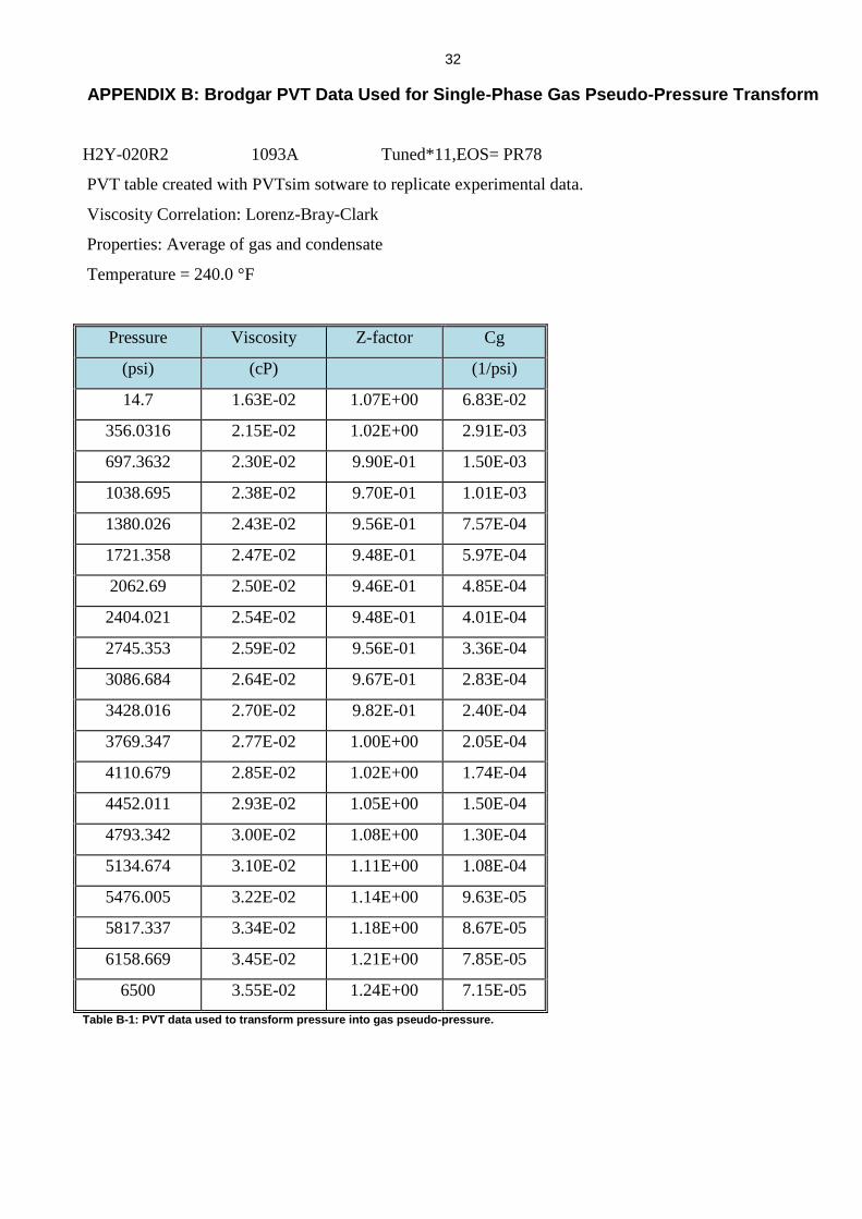
32

APPENDIX B: Brodgar PVT Data Used for Single-Phase Gas Pseudo-Pressure Transform

H2Y-020R2 1093A Tuned*11,EOS= PR78

PVT table created with PVTsim sotware to replicate experimental data.

Viscosity Correlation: Lorenz-Bray-Clark

Properties: Average of gas and condensate

Temperature = 240.0 °F

Pressure Viscosity Z-factor Cg

(psi) (cP) (1/psi)

14.7 1.63E-02 1.07E+00 6.83E-02

356.0316 2.15E-02 1.02E+00 2.91E-03

697.3632 2.30E-02 9.90E-01 1.50E-03

1038.695 2.38E-02 9.70E-01 1.01E-03

1380.026 2.43E-02 9.56E-01 7.57E-04

1721.358 2.47E-02 9.48E-01 5.97E-04

2062.69 2.50E-02 9.46E-01 4.85E-04

2404.021 2.54E-02 9.48E-01 4.01E-04

2745.353 2.59E-02 9.56E-01 3.36E-04

3086.684 2.64E-02 9.67E-01 2.83E-04

3428.016 2.70E-02 9.82E-01 2.40E-04

3769.347 2.77E-02 1.00E+00 2.05E-04

4110.679 2.85E-02 1.02E+00 1.74E-04

4452.011 2.93E-02 1.05E+00 1.50E-04

4793.342 3.00E-02 1.08E+00 1.30E-04

5134.674 3.10E-02 1.11E+00 1.08E-04

5476.005 3.22E-02 1.14E+00 9.63E-05

5817.337 3.34E-02 1.18E+00 8.67E-05

6158.669 3.45E-02 1.21E+00 7.85E-05

6500 3.55E-02 1.24E+00 7.15E-05

Table B-1: PVT data used to transform pressure into gas pseudo-pressure.

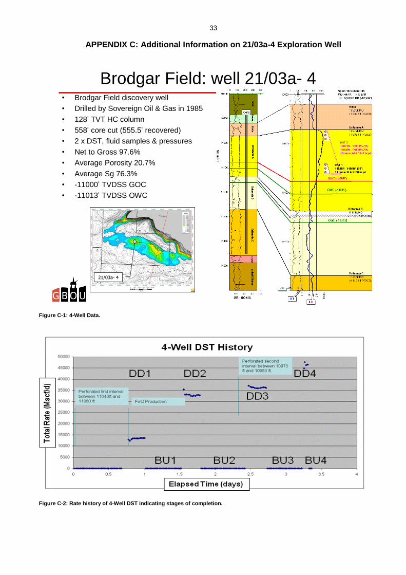
33

APPENDIX C: Additional Information on 21/03a-4 Exploration Well

Brodgar Field: well 21/03a- 4• Brodgar Field discovery well

• Drilled by Sovereign Oil & Gas in 1985

• 128’ TVT HC column

• 558’ core cut (555.5’ recovered)

• 2 x DST, fluid samples & pressures

• Net to Gross 97.6%

• Average Porosity 20.7%

• Average Sg 76.3%

• -11000’ TVDSS GOC

• -11013’ TVDSS OWC

21/03a- 4

Figure C-1: 4-Well Data.

Figure C-2: Rate history of 4-Well DST indicating stages of completion.

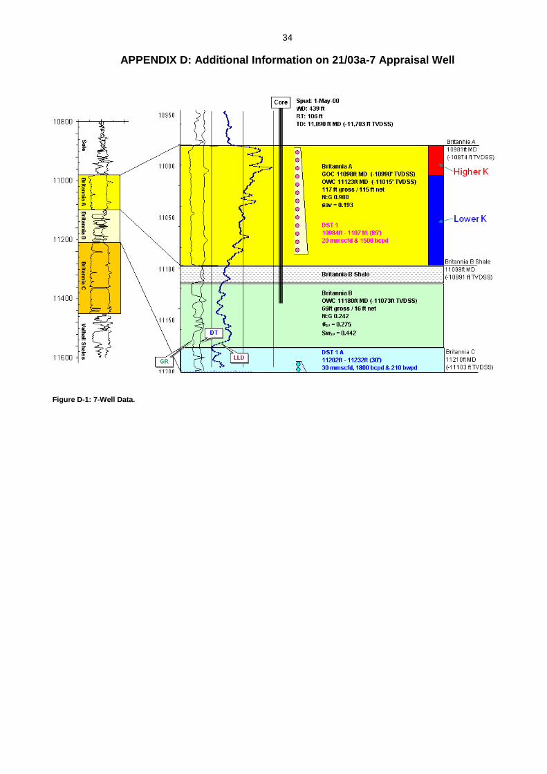
34

APPENDIX D: Additional Information on 21/03a-7 Appraisal Well

Figure D-1: 7-Well Data.

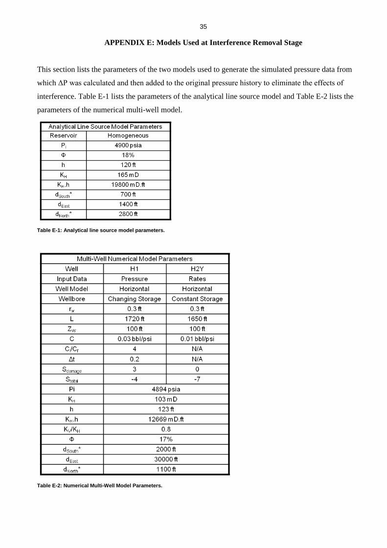
35

APPENDIX E: Models Used at Interference Removal Stage

This section lists the parameters of the two models used to generate the simulated pressure data from

which ΔP was calculated and then added to the original pressure history to eliminate the effects of

interference. Table E-1 lists the parameters of the analytical line source model and Table E-2 lists the

parameters of the numerical multi-well model.

Table E-1: Analytical line source model parameters.

Table E-2: Numerical Multi-Well Model Parameters.

Documents

Title Page IMPERIAL COLLEGE LONDON Department of Earth ...Title Page IMPERIAL COLLEGE LONDON Department of Earth Science and Engineering Centre for Petroleum Studies Brodgar Downhole