Titre: Integrated model for comparison of one-and two-pipe

Titre:Title:

Integrated model for comparison of one- and two-pipe ground-coupled heat pump network configurations

Auteurs:Authors: Laurent Gagné-Boisvert et Michel Bernier

Date: 2018

Type: Article de revue / Journal article

Référence:Citation:

Gagné-Boisvert, L. & Bernier, M. (2018). Integrated model for comparison of one- and two-pipe ground-coupled heat pump network configurations. Science and Technology for the Built Environment, 24(7), p. 726-742. doi:10.1080/23744731.2017.1366184

Document en libre accès dans PolyPublieOpen Access document in PolyPublie

URL de PolyPublie:PolyPublie URL: http://publications.polymtl.ca/2778/

Version: Version finale avant publication / Accepted versionRévisé par les pairs / Refereed

Conditions d’utilisation:Terms of Use: Tous droits réservés / All rights reserved

Document publié chez l’éditeur officielDocument issued by the official publisher

Titre de la revue:Journal Title: Science and Technology for the Built Environment (vol. 24, no 7)

Maison d’édition:Publisher: Taylor & Francis

URL officiel:Official URL: https://doi.org/10.1080/23744731.2017.1366184

Mention légale:Legal notice:

This is an Accepted Manuscript of an article published by Taylor & Francis in Science and Technology for the Built Environment on 2018-08-30, available online: http://www.tandfonline.com/10.1080/23744731.2017.1366184

Ce fichier a été téléchargé à partir de PolyPublie, le dépôt institutionnel de Polytechnique Montréal

This file has been downloaded from PolyPublie, theinstitutional repository of Polytechnique Montréal

http://publications.polymtl.ca

https://doi.org/10.1080/23744731.2017.1366184

http://publications.polymtl.ca/2778/

https://doi.org/10.1080/23744731.2017.1366184

http://www.tandfonline.com/10.1080/23744731.2017.1366184

http://publications.polymtl.ca/

Integrated Model for Comparison of One- and Two-pipe GCHP Network

Configurations

by

Laurent Gagné-Boisvert, Student member ASHRAE

and

Michel Bernier1, PE, Ph.D., Fellow ASHRAE

Polytechnique Montréal

Department of Mechanical Engineering

Accepted for publication in

Science and Technology for the Built Environment

July 2017

1 Corresponding author: Tel.: +1-514-340-4711; e-mail address: [email protected].

Laurent Gagné-Boisvert is a M.A.Sc. student in the Department of Mechanical Engineering, Polytechnique Montreal, Montreal, Quebec, Canada. Michel Bernier is a professor in the Department of Mechanical Engineering, Polytechnique Montreal, Montreal, Quebec, Canada.

Integrated Model for Comparison of One- and Two-pipe GCHP Network Configurations

Abstract

Several network configurations are possible when designing the interior portion of

centralized ground-coupled heat pump (GCHP) systems. In this study, three different

configurations are examined: Two-pipe networks with either a direct-return or a reverse-

return and one-pipe systems. One-pipe networks typically require less piping than two-pipe

systems. However, heat pump energy consumption might be higher because the inlet

temperature to the heat pumps tends to increase (in cooling) or decrease (in heating) along

the network. In this work, a versatile integrated modelling tool is developed in the

TRNSYS environment to study the energy consumption (pumps and heat pumps) of each

type of network. A control method for one-pipe systems, based on the bore field return

temperature, is also proposed. The tool is first compared to detailed individual models in

annual simulations where it is shown to give good results. The results obtained with four

different case studies indicate that the total annual energy consumption of one-pipe

networks is up to 5% higher than two-pipe networks even though the pumping energy is 4

to 53% lower than two-pipe networks. No significant differences are observed in the

required borehole length.

Introduction

There are several possible piping configurations when designing the interior portion of

centralized ground-coupled heat pump (GCHP) systems. Three of these configurations are

studied in this paper. They are presented schematically in Figure 1. In the reverse-return

two-pipe network (Figure 1a), heat pumps are piped in parallel and have the same inlet

fluid temperature. One of the main advantage of these systems is that they are somewhat

easier to balance, since each parallel circuit has more or less the same pressure drop.

However, a supplementary return pipe might be required if the heat pumps are positioned

in-line as presented in Figure 1a. It is possible to avoid the supplementary pipe if heat

pumps are positioned such that the circuit forms a loop. Finally, variable flow pumping can

be used to reduce pumping energy consumption.

In direct-return two-pipe networks (Figure 1b), heat pumps are also piped in parallel but

the flow out of the first heat pump is the first to be returned to the main pump, thereby

eliminating the need for a supplementary return pipe. Each circuit has a different pressure

drop and balancing valves are typically required to maintain the desired flow rate in each

heat pump. Variable flow pumping can also be used to reduce energy consumption.

In one-pipe networks, each heat pump draws and rejects fluid from and to the same primary

pipe (Figure 1c). The main flow rate, controlled to maintain a favorable bore field return

temperature, is constant along the primary pipe while individual circulator pumps are

typically activated in tandem with their corresponding heat pump. Heat pumps are operated

in series each with a different inlet temperature as the primary pipe fluid temperature is

influenced by the operation of the previous units. If all heat pumps are operating in cooling

(or heating), heat pumps located towards the end of the loop will receive a less favourable

inlet temperature leading to higher heat pump energy consumption. However, one-pipe

systems are known to be simpler to design and operate with reduced piping costs.

This paper proposes a tool to perform annual simulations of one- or two-pipe networks to

evaluate the annual operating energy costs related to pumping and heat pumps. The tool

integrates into a single TRNSYS Type: heat pump modelling, pressure drop calculations

through pipes and valves, as well as pump and circulator calculations. The paper is

subdivided into several sections. First, the features and operation of the three networks are

reviewed. Then, the modelling methodologies used in the tool are presented. This is

followed by a comparison between results obtained using the integrated tool and a detailed

simulation involving individual models. Finally, four case studies are presented and

analysed in the application section.

Figure 1a, b and c: Reverse-return Two-pipe (left), Direct-return Two-pipe (center) and One-pipe (right) GCHP networks with connection diagram.

Literature review

Several piping strategies are possible for centralized GCHP systems, including one-pipe

systems (Boldt and Keen, 2015). Stethem (1994) re-examined hydronic one-pipe systems,

which were common around 1950 (Stethem, 1995). He points out the advantages

associated with reduced piping needs and a decrease in the energy consumption which

result from the use of fewer valves and the decoupling of the primary and secondary loops.

Application to GCHP systems was not specifically addressed. However, he stated that one-

pipe networks are efficient in high-rise buildings and schools using heat pumps.

Kavanaugh and McInerny (2001) showed that the selection of a pumping strategy

influences pumping energy consumption. Kavanaugh et al. (2003) found that decentralized

systems relying on on/off circulators require less energy for low to moderate occupancy

buildings (less than 60 hours/week), centralized systems with a variable-speed pump being

a close second. Their study, based on simple bin calculations, also concluded that these

centralized systems are the most efficient for high occupancy buildings (over 60

hours/week).

Bernier et al. (2005) presented a methodology to compare the energy consumption and life-

cycle costs of centralized and decentralized GCHP pumping systems. They stated that

pumping costs over 20 years are lower for centralized systems while overall costs are lower

for decentralized systems due to expensive piping required in centralized systems.

Heat Pump

Bore Field

Sup

ple

men

tary

pip

e le

ngt

h

Two-Pipe Reverse-Return

Heat Pump

Heat Pump

Heat Pump

BallControl

VFDMech.Room

1

4

0

2

3

5

8

6

7

9 10

1112 13 Heat

Pump

Bore Field

Two-Pipe Direct-Return

Heat Pump

Heat Pump

Heat Pump

VFDMech.Room

Balance

Balance

Balance

Balance 1

4

0

2

3

8

5

7

6

9 10

11

12 13

14

Heat Pump

Bore Field

One-Pipe

Heat Pump

Heat Pump

Heat Pump

VFDMech.Room

Check

1

0

5

7 8

2

3 4

6

However, this study did not account for the total required borehole length which is typically

longer for decentralized systems that cannot take advantage of load diversity.

Cunniff and Zerba (2006) stated that one-pipe systems use small circulators to replace the

expensive and energy-consuming control valves and balancing valves. They concluded that

circulators deliver the fluid to where it is needed, instead of forcing it where it is not needed

resulting in reduced piping and installation costs as well as energy savings. One-pipe

networks coupled to fan coil units have been shown to be energy efficient and cost effective

in a residential tower retro-fit (Cunniff, 2011).

Mescher (2009) stated that GCHP one-pipe systems are less expensive and more energy

efficient than two-pipe systems and that their design, installation and balancing are simpler.

A two-pipe network requires additional pipes, fittings, piping size reductions and insulation

compared to a one-pipe system. He shows that a one-pipe system equipped with two

parallel constant speed pumps has lower pumping and total energy consumption than a

two-pipe system with a single variable-speed pump. He also specified that the selection of

a one-pipe system in actual building retrofits led to piping installation cost savings of $0.50

to $1.50/ft2 ($5.38 to $16.15/m2). He mentioned that one-pipe systems can be almost as

energy efficient as decentralized unitary loops with the added benefit that one-pipe

networks can potentially lead to shorter boreholes because of load diversity.

Kavanaugh (2011) performed a GCHP systems survey and found that one-pipe systems

presented the highest Energy Star ratings along with decentralized unitary loops. He

specified that five 1950s schools that were retrofitted with one-pipe GCHP systems

obtained an average Energy Star rating of 96. He also proposed to add a third smaller

parallel main pump providing flow up to a 25% part-load operation in one-pipe systems to

reduce energy consumption. However, using a variable-speed main pump in one-pipe

systems has not been assessed.

Until recently, circulators had typical wire-to-water efficiencies around 20 to 25%

(Kavanaugh and Rafferty, 2014). These relatively low efficiencies made their use less

attractive in one-pipe systems. However, circulator efficiency nearly doubled in recent

years (Bidstrup, 2012). Gagné-Boisvert and Bernier (2017) looked at commercially

available circulators and proposed three sets of curves for low, high and best efficiencies

(Figure 2). As shown on this figure, circulator efficiency has improved substantially.

Figure 2: Overall wire-to-water efficiencies of commercially available circulators (Gagné-Boisvert and Bernier, 2017).

In summary, the literature survey indicates that there are advantages in using one-pipe

systems. However, there are no systematic studies that compared one-pipe networks to

conventional direct-return and reverse-return networks. It is the objective of this study to

develop a modelling tool that can perform annual simulations to assess the performance of

these three systems.

Network features and operation

Piping lengths and diameters are different for each network. In a reverse-return system, the

supply pipe section out of the bore field (segment 10-1 in Figure 1a) has the largest

diameter as it must handle the full flow. The supply pipe flow rate then decreases along the

network (from 1 to 4) and so does the diameter. The supply pipe section for the last heat

pump (3-4) has the smallest diameter. The flows in the return pipe are symmetrical to the

flows in the supply pipe as they increase from 5 to 8. Hence, the return pipe after the last

heat pump (8-9) has the largest diameter because it handles the full flow.

In a direct-return system (Figure 1b), the return pipe flow rate decreases along the network

in phase with the supply pipe (from 8 to 5). Then, the first pipe section has the largest

supply and return pipe diameters (10-1 and 8-9).

Finally, in a one-pipe system, the primary pipe has typically the same diameter from

beginning to end removing the need for reduction fittings. One of the main advantage of a

one-pipe system is that its interior primary pipe is up to 50% shorter than with a reverse-

return two-pipe system. Kavanaugh (2011) and Mescher (2009) also stated that simpler

systems, such as one-pipe systems, tend to be more energy efficient over time. The average

diameter is typically larger than for two-pipe systems. However, overall piping costs are

generally lower for one-pipe systems. Finally, one-pipe systems require a circulator for

each heat pump (5-6) which is not the case for two-pipe networks.

The design and operation of a two-pipe network is relatively more complex with motorized

isolation valves, strainers, inverters and differential pressure controls (Mescher, 2009).

Additional pipes, fittings, and pipe insulation are also required compared to a one-pipe

system. Balancing valves (flow control) must also be added in direct-return systems (Duda,

2015) while they are generally not required in reverse-return systems (Taylor and Stein,

2002).

Table 1 presents a summary of the basic components required in each network as presented

by Mescher (2009) and Taylor and Stein (2002). This selection may differ depending on

the designer. Hose kits are assumed to be installed on each heat pump. They are positioned

between connections 11 and 12 for two-pipe systems (Figures 1a and b) and between

connections 6 and 7 for one-pipe systems (Figure 1c). An on/off control valve (often called

a zone valve) is required (as shown between 12-13 in Figures 1a and b) at each heat pump

in two-pipe networks to stop the flow when the heat pump is not operating. Direct-return

systems need a balancing valve for each unit to allow the right flow to be supplied in each

different hydraulic path (14-11 in Figure 1b). It is also common practice to install ball

valves to isolate each heat pump branch from the primary pipe. However, as presented in

Figure 1c, one-pipe networks require only one ball valve (1-5) since a check valve is added

(7-8) (Mescher, 2009).

All these fittings induce pressure drops that need to be properly accounted to determine

pumping energy consumption. The concept of flow coefficients (𝐶𝑣) is used here to

evaluate valve and hose pressure drops (Kavanaugh and Rafferty, 2014). The last column

in Table 1 shows 𝐶𝑣 values used in the present work. These values are typical for a 3-ton

heat pump unit, which is a frequently used capacity (Kavanaugh and Gray, 2016). For

example, 𝐶𝑣 values are equal to 25 for the two-way control valve and 8 for the hoses (based

on flows in gpm and a 1 psi (6.9 kPa) pressure drop). Using the definition of 𝐶𝑣

(=𝑓𝑙𝑜𝑤/√∆𝑝 ) where the flow is in gpm and the ∆𝑝 is in psi, the pressure drop is equal,

respectively, to 0.13 and 1.3 psi (0.9 and 8.7 kPa) for the control valve and the connecting

hoses for a 9 gpm flow rate (3 gpm/ton). A 3-ton capacity heat pump is used as the reference

capacity in the proposed modelling tool; 𝐶𝑣 are scaled for other capacities as explained

later.

Table 1: One- and two-pipe network components.

Equipment Components per heat pump Cv

One-pipe**

Two-pipe reverse-return***

Two-pipe direct-return**/***

Selected for 3-ton HP

Hose kit 1 1 1 8* On/off control valve 1 1 25* Shut-off ball valve 1 2 2 23.5* Balancing valve 1 5.2** Check valve 1 21* Circulator 1 *Kavanaugh and Rafferty (2014), **Mescher (2009), ***Taylor and Stein (2002)

In all cases considered in this paper, the main pump is equipped with a variable frequency

drive (VFD). The resulting variable-speed pump can then modulate the flow rate to reduce

pumping power. Modulation is based here on differential pressure for two-pipe networks

and on bore field return temperature for one-pipe networks, respectively. VFD can usually

decrease the main pump flow rate up to a minimum percentage of the nominal flow. The

main pump also shuts down if no heat pumps are in operation.

For two-pipe networks, the main flow is a function of the number of heat pumps in

operation, as shown in Figure 3a. The main flow decreases linearly as a function of the

required flow to the heat pumps up to a certain minimum (30% in this case) after which

the main flow rate remains constant. The VFD regulates the main pump speed based on the

signal generated by a differential pressure switch measuring the pressure difference

between the inlet and outlet of the farthest heat pump branch (between points 4 and 8 in

Figure 1a). The differential pressure switch set point is generally set to the pressure drop

in a heat pump branch at nominal flow. Each heat pump is equipped with a motorized two-

way control valve which closes when the heat pump is off. When a heat pump is turned

off, more flow will be supplied to other units, increasing momentarily the differential

pressure in each operating heat pump branch. In turn, this induces a reduction of the VFD

speed to supply each heat pump with its required flow. This common two-pipe control

strategy requires a similar pressure drop in each parallel branch, which is achieved by

adding balancing valves in direct-return networks. The balancing valve, which is frequently

an automatic flow limiting valve (Mescher, 2009), allows a specific flow to a heat pump.

If too much flow is supplied to a balancing valve after another unit shut-off, its pressure

drop increases to limit the flow, increasing the differential pressure and reducing the VFD

speed. Balancing valves are useful devices but present higher pressure drop compared to

other valves, even when fully opened. More details on hydronic balancing and balancing

valves are given by Taylor and Stein (2002).

Figure 3a, b: Typical fraction of the main flow as a function of the number of operating heat pumps for two-pipe

network (left) and of the bore field return temperature for one-pipe network (right).

In two-pipe networks, if the operating heat pumps require a smaller total flow rate than the

lower limit of the VFD, heat pump branch differential pressure will increase. The

supplementary flow is then bypassed as presented by Taylor and Stein (2002) and

recombined with the flow exiting all the heat pumps.

In a one-pipe system, the main flow is not a function of the number of operating units like

for two-pipe systems. It is typically controlled to maintain a favorable bore field return

temperature. However, no guidelines could be found in the literature regarding the range

of acceptable bore field return temperatures. A control method is therefore proposed in this

paper and is illustrated in Figure 3b. This figure presents the required flow rate for the

expected temperature span where TtoHP,min, TtoHP,max and ∆T are operational variables. The

main flow control method proposed here is a function of the fluid temperature exiting the

main pump and entering the first heat pump, TtoHP. If TtoHP reaches the high (TtoHP,max) or

low (TtoHP,min) operating temperature limits (e.g. 0 °C or 35 °C as shown in Fig. 3b), the

VFD must provide 100% of the maximum flow. If TtoHP is between TtoHP,min+∆T and

TtoHP,max -∆T, the VFD is set to supply its minimum flow to reduce pumping power. The

flow varies linearly between minimum and maximum values, as shown in Figure 3b. With

this control scheme, the value of ∆T has to be correctly specified to reduce energy

consumption. A high ∆T increases the main pump energy consumption as higher flow rates

are required on average. On the other hand, heat pump energy consumption is reduced as

higher flow rates lead to more favorable bore field return temperature and less temperature

changes between heat pumps. Based on the four test cases which will be presented later,

the total energy consumption is minimized when ∆T = 6 °C.

Integrated modelling tool

It is possible to model and simulate piping networks of GCHP systems in simulation

software tools such as TRNSYS. However, it becomes impractical and time consuming

when there is a large number of heat pumps, valves, pipes to link together. Furthermore,

for comparative studies, different assemblies need to be constructed for the one-pipe,

reverse-return two-pipe and direct-return two-pipe networks.

In order to make these comparisons simpler and faster, a general integrated modelling tool

has been developed to compare the energy performances of GCHP systems with one- or

two-pipe interior networks. The tool is developed in the TRNSYS v17 environment (Klein

et al., 2010) in the form of a single Type. It needs to be linked to a main circulating pump

model and a bore field model.

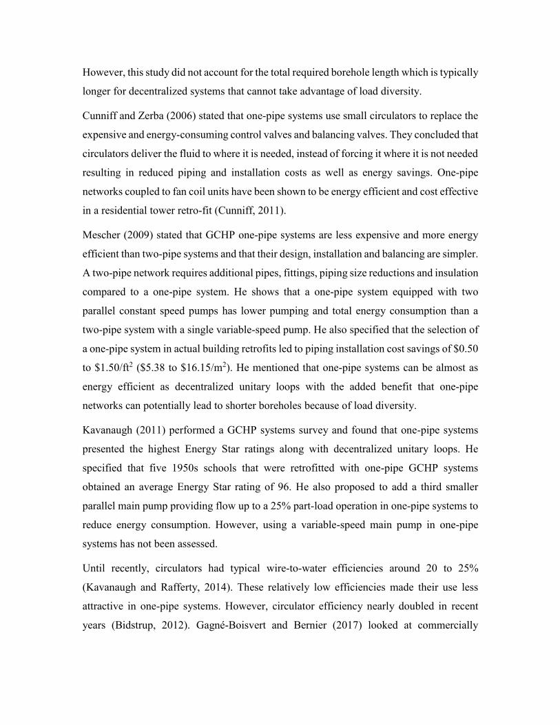
The parameters, inputs and outputs of the Type are presented in Figure 4. They are also

described in more details in Table 7 in Appendix A. The user can modify several

parameters including the type of network, the pipe linear head loss, heat pump COPs, and

valve 𝐶𝑣. Heat pump spatial coordiantes (X,Y), nominal heat pump capacity (tons) and

required flow rate (gpm/ton) are also user-selected. Building loads associated with each

heat pump (Load (i) in Figure 4) are inputs to the Type. Typically, these loads are given on

an hourly basis but other time steps can be used. The assumptions, the methodology and

some intermediate results obtained with this tool will now be presented.

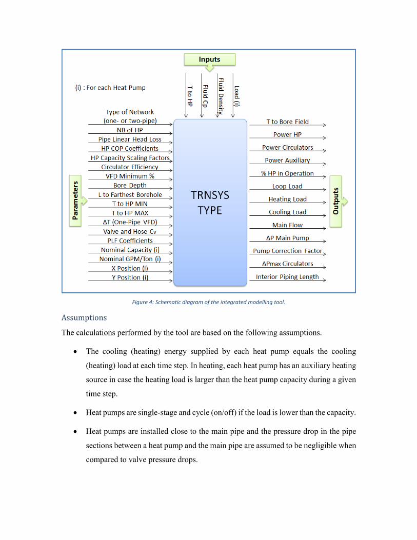
Figure 4: Schematic diagram of the integrated modelling tool.

Assumptions

The calculations performed by the tool are based on the following assumptions.

The cooling (heating) energy supplied by each heat pump equals the cooling

(heating) load at each time step. In heating, each heat pump has an auxiliary heating

source in case the heating load is larger than the heat pump capacity during a given

time step.

Heat pumps are single-stage and cycle (on/off) if the load is lower than the capacity.

Heat pumps are installed close to the main pipe and the pressure drop in the pipe

sections between a heat pump and the main pipe are assumed to be negligible when

compared to valve pressure drops.

Each parallel heat pump segment, comprising valves and hose kit, has the same

pressure drop.

The main pipe follows the shortest path between each successive heat pump.

Pipes and U-tubes in boreholes are designed so that the nominal linear pressure

drop is the same everywhere in the network. A default value of 2 ft wc/100 feet of

pipe is assumed.

The reference heat pump has a 3-ton (10.6 kW) nominal capacity.

All heat pumps have the same normalized performance and capacity curves as the

reference heat pump. These values depend only on the entering fluid temperature

(Hackel et al., 2008).

Methodology

Main flow control

The maximum main flow rate, �̇�𝑡𝑜𝑡, is the sum of the nominal flow rate of each heat pump,

�̇�𝑖 (Eq. 1). It is then multiplied by the VFD fraction, 𝑓, which varies between the minimum

fraction (𝑓𝑚𝑖𝑛) and 100%, to obtain the main flow rate, �̇�, during a given time step (Eq.

2).

In one-pipe systems, the scenario proposed in Figure 3b is used to determine the VFD

fraction for one-pipe systems, 𝑓1𝑝𝑖𝑝𝑒, based on the input value of TtoHP prevailing during a

given time step.

The VFD fraction for two-pipe systems, 𝑓2𝑝𝑖𝑝𝑒, is a function of the number of heat pumps

in operation during a time step and their corresponding nominal flow rates (Eq. 3). The

heat pump nominal flow rate is defined as the heat pump nominal capacity (in tons)

multiplied by its specific flow rate per ton. If the VFD fraction is inferior to the minimum

flow fraction, then 𝑓2𝑝𝑖𝑝𝑒 is set to 𝑓𝑚𝑖𝑛. As indicated earlier, the superfluous flow is then

bypassed and recombined with the fluid exiting all the heat pumps (Taylor and Stein,

2002).

�̇�𝑡𝑜𝑡 = ∑ �̇�𝑖 (1)

�̇� = 𝑓 × �̇�𝑡𝑜𝑡 (2)

𝑓2𝑝𝑖𝑝𝑒 = 𝑀𝐴𝑋 [𝑓𝑚𝑖𝑛 ,∑ �̇�𝑖

𝑂𝑝𝑒𝑟𝑎𝑡𝑖𝑛𝑔 𝐻𝑃𝑖

�̇�𝑡𝑜𝑡] (3)

Heat pump locations and piping lengths

The selection of one of the three networks influences the interior piping length, which

affects the pressure drop. The tool must then account for heat pump location to evaluate

the various pipe lengths and uses the following procedure to do so. As shown in Figure 5,

each numbered heat pump is located with (X,Y) coordinates which are set as parameters in

the TRNSYS Type (Figure 4). By convention, the mechanical room and main circulating

pump are located at coordinate (0,0). Then, the shortest length between each element (heat

pump or mechanical room) is calculated.

Figure 5: Example of heat pump locations in a building.

The length used to calculate the worst hydraulic path, which determines the overall piping

pressure drop, is then evaluated. It includes the length of the supply and return pipes

between the mechanical room and the last heat pump, the length of the supply and return

pipes to the farthest borehole, and the length of the upward and downward legs in a

borehole.

HP3

Mech. RoomHP2

HP4

HP1

(X3,Y3)

(X1,Y1)

(0,0)

HP10

(X10,Y10)

HP9

HP8

HP7

HP5

(X5,Y5)

HP6

(X6,Y6)

(X4,Y4)

(X2,Y2) (X9,Y9)

(X8,Y8)

(X7,Y7)

Head losses

The main pump head, 𝐻, is a function of the supplied flow rate and installed accessories

with their associated pressure drops (Table 1). It is specific to the chosen configuration and

varies over time. The tool calculates the main pump head at each time step which is then

outputted along with the main flow rate to a TRNSYS pump model to evaluate pumping

energy consumption.

In two-pipe systems, each operating parallel branch has the same pressure drop. The main

pump head is then the sum of the pressure drop in a heat pump branch (heat pump and

associated valves in its supply and return pipe segments), and in the main pipe and

borehole. In a reverse-return network like the one presented in Figure 1a, the main pump

nominal head when all heat pumps are in operation, 𝐻2𝑝𝑖𝑝𝑒,𝑟𝑒𝑣, is calculated according to

Equation 4.

𝐻2𝑝𝑖𝑝𝑒,𝑟𝑒𝑣 = ∆𝑝1−2 + ∆𝑝2−3 + ∆𝑝3−4 + ∆𝑝4−8 + ∆𝑝8−9 + ∆𝑝9−10 + ∆𝑝10−1 (4)

where ∆𝑝8−9 and ∆𝑝10−1 are related to the main pipe segments with the largest diameter

and total flow. They also include the pipe length from the mechanical room to the farthest

borehole. ∆𝑝9−10 is the sum of the pressure drop through the upward and downward legs

of a U-tube borehole. ∆𝑝1−2, ∆𝑝2−3, and ∆𝑝3−4 are related to the supply pipe of the last

heat pump. The nominal pressure drop in each of these segments is equal to its length

multiplied by the nominal linear head loss which is based on the maximum design flow

and provided as a parameter to the TRNSYS Type. ∆𝑝4−8, calculated by Equation 5, is the

pressure drop in a heat pump branch.

∆𝑝4−8 = ∆𝑝4−11 + ∆𝑝11−𝐻𝑃 + ∆𝑝𝐻𝑃 + ∆𝑝𝐻𝑃−12 + ∆𝑝12−13 + ∆𝑝13−8 (5)

∆𝑝4−11 and ∆𝑝13−8 are equal and represent the pressure drop in both ball valves while

∆𝑝12−13 is the two-way control valve pressure drop. The sum of ∆𝑝11−HP and ∆𝑝HP−12

represents the hose kit pressure drop. Valve and hose pressure drops are calculated using

flow coefficients and Equation 6, where ∆𝑝Valve is in kPa and �̇�𝑖 is in L/s. Components

and their specific 𝐶𝑣 are selected for a 3-ton heat pump operating with the standard 3

gpm/ton flow rate. These values are set as parameters in the TRNSYS Type. If a specific

heat pump has a different nominal capacity, 𝐶𝐴𝑃𝑛𝑜𝑚, it requires a different flow rate and

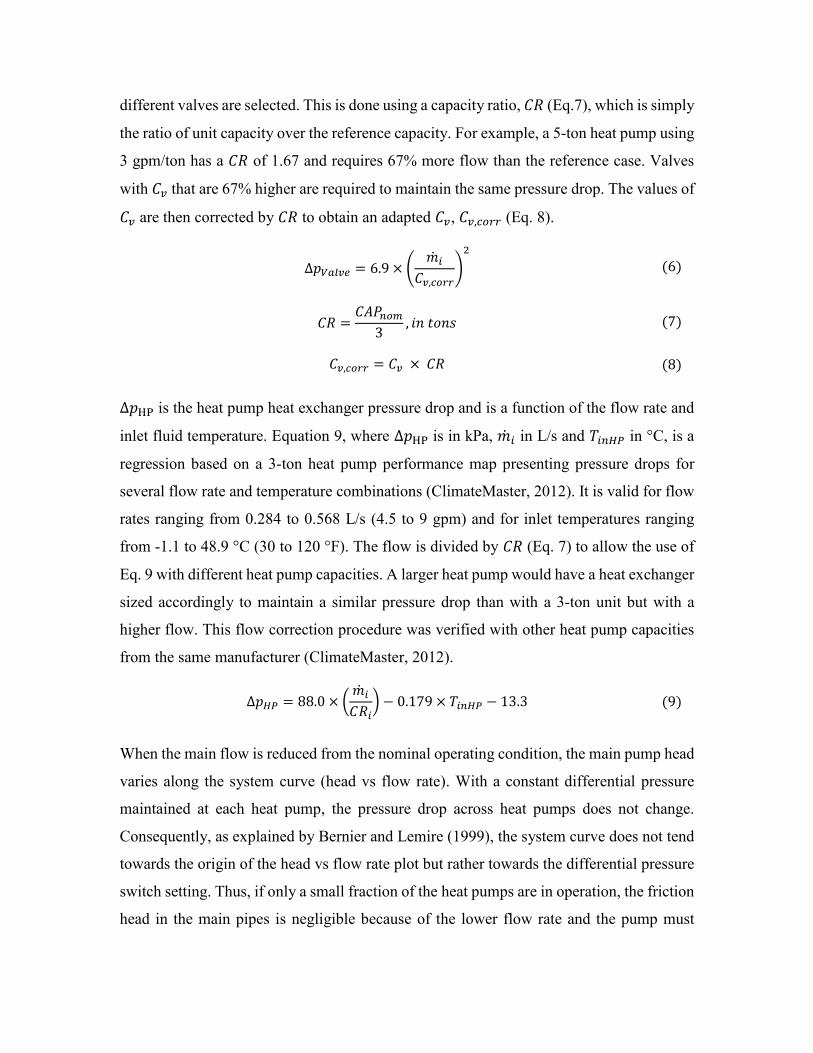
different valves are selected. This is done using a capacity ratio, 𝐶𝑅 (Eq.7), which is simply

the ratio of unit capacity over the reference capacity. For example, a 5-ton heat pump using

3 gpm/ton has a 𝐶𝑅 of 1.67 and requires 67% more flow than the reference case. Valves

with 𝐶𝑣 that are 67% higher are required to maintain the same pressure drop. The values of

𝐶𝑣 are then corrected by 𝐶𝑅 to obtain an adapted 𝐶𝑣, 𝐶𝑣,𝑐𝑜𝑟𝑟 (Eq. 8).

∆𝑝𝑉𝑎𝑙𝑣𝑒 = 6.9 × (�̇�𝑖

𝐶𝑣,𝑐𝑜𝑟𝑟)

2

(6)

𝐶𝑅 =𝐶𝐴𝑃𝑛𝑜𝑚

3, 𝑖𝑛 𝑡𝑜𝑛𝑠 (7)

𝐶𝑣,𝑐𝑜𝑟𝑟 = 𝐶𝑣 × 𝐶𝑅 (8)

∆𝑝HP is the heat pump heat exchanger pressure drop and is a function of the flow rate and

inlet fluid temperature. Equation 9, where ∆𝑝HP is in kPa, �̇�𝑖 in L/s and 𝑇𝑖𝑛𝐻𝑃 in °C, is a

regression based on a 3-ton heat pump performance map presenting pressure drops for

several flow rate and temperature combinations (ClimateMaster, 2012). It is valid for flow

rates ranging from 0.284 to 0.568 L/s (4.5 to 9 gpm) and for inlet temperatures ranging

from -1.1 to 48.9 °C (30 to 120 °F). The flow is divided by 𝐶𝑅 (Eq. 7) to allow the use of

Eq. 9 with different heat pump capacities. A larger heat pump would have a heat exchanger

sized accordingly to maintain a similar pressure drop than with a 3-ton unit but with a

higher flow. This flow correction procedure was verified with other heat pump capacities

from the same manufacturer (ClimateMaster, 2012).

∆𝑝𝐻𝑃 = 88.0 × (�̇�𝑖

𝐶𝑅𝑖) − 0.179 × 𝑇𝑖𝑛𝐻𝑃 − 13.3 (9)

When the main flow is reduced from the nominal operating condition, the main pump head

varies along the system curve (head vs flow rate). With a constant differential pressure

maintained at each heat pump, the pressure drop across heat pumps does not change.

Consequently, as explained by Bernier and Lemire (1999), the system curve does not tend

towards the origin of the head vs flow rate plot but rather towards the differential pressure

switch setting. Thus, if only a small fraction of the heat pumps are in operation, the friction

head in the main pipes is negligible because of the lower flow rate and the pump must

deliver a head equivalent to the differential pressure switch setting. The system then

behaves like an open system with a static head.

The pressure drop in every pipe segment, ∆𝑝𝑠, varies with flow rate according to the

assumption presented earlier. Thus, as shown in Eq. 10, the nominal pressure drop of each

pipe segment (𝐻𝑙𝑖𝑛𝑒𝑎𝑟) is multiplied by the square of the fraction of the nominal flow in

that segment, �̇�𝑠/�̇�𝑛𝑜𝑚, and by its length, 𝐿, to obtain ∆𝑝𝑠. Similarly, the pressure drop in

boreholes and in segments containing the main flow is the product of the nominal pressure

drop and the square of the flow fraction.

∆𝑝𝑠 = 𝐿 × 𝐻𝑙𝑖𝑛𝑒𝑎𝑟(�̇�𝑠/�̇�𝑛𝑜𝑚)2 (10)

The flow rate varies between heat pumps in the supply and return main pipes. This irregular

flow distribution in the supply and return pipes is considered in the tool as the flow in each

segment is compared to its nominal flow at each time step.

For example, and with reference to Figure 1a, if only the first and third heat pumps are in

operation during a time step, the main flow will be 50% of the nominal flow (assuming

that all heat pumps have the same nominal flow rate). The main pump head, 𝐻2𝑝𝑖𝑝𝑒,𝑟𝑒𝑣′, is

then given by Eq. 11 representing the hydraulic path to the farthest operating heat pump.

The heat pump branch pressure drop, ∆𝑝3−7, which includes the third heat pump, is equal

to Eq. 5 while pipe segments are different. The flow rate in segments 8-9, 9-10 and 10-1 is

50% of the nominal flow rate, leading to a pressure drop equal to 25% of the nominal

pressure drop in these segments. Moreover, ∆𝑝7−8 is equal to 44% of this segment nominal

pressure drop as it handles the return flow of two heat pumps instead of three.

𝐻2𝑝𝑖𝑝𝑒,𝑟𝑒𝑣′ = ∆𝑝1−2 + ∆𝑝2−3 + ∆𝑝3−7 + ∆𝑝7−8 + ∆𝑝8−9 + ∆𝑝9−10 + ∆𝑝10−1 (11)

The main pump head in a direct-return system is evaluated the same way except for the

balancing valve pressure drop which is added to the heat pump branch head loss. Different

pipe segments are also considered as the hydraulic path is different.

Finally, in one-pipe systems, there are two different head losses to consider. The primary

loop head (main pipe and boreholes) is handled by the main pump while the heat pump

branch head (heat pump and valves) is handled by each circulator. For example, based on

the geometry of Figure 1c, the main pump nominal head, 𝐻1𝑝𝑖𝑝𝑒, is calculated using Eq.

12. It is then equal to the total hydraulic path length multiplied by the nominal linear head

loss. With a reduced main flow, this head is multiplied by the square of the main flow

fraction as described earlier in Eq. 10.

𝐻1𝑝𝑖𝑝𝑒 = ∆𝑝1−2 + ∆𝑝2−3 + ∆𝑝3−4 + ∆𝑝4−1 (12)

The heat pump branch pressure drops are calculated with an equation similar to Eq. 5 but

with different valves (see Table 1). The heat pump branch pressure drop is independent

from the main flow. This pressure drop is calculated for each operating heat pump branch

so that individual circulator pumping power, 𝑊𝐶𝑖𝑟𝑐𝑖, can be obtained (Eq. 13). Circulator

efficiencies, 𝜂𝑖, are based on regressions presented in Figure 2. The user can select which

class (Low, High or Best Efficiency) to use.

𝑊𝐶𝑖𝑟𝑐𝑖=

�̇�𝑖 × ∆𝑝𝑖

𝜂𝑖 (13)

Heat Pump COP and Capacity

The fluid inlet temperature influences heat pump COP and capacity. In two-pipe systems,

it is assumed that all units have the same inlet fluid temperature during a given time step.

Consequently, based on the assumption mentioned above, they also have the same

normalized capacity and COP. However, in a one-pipe system, normalized capacity and

COP vary since the fluid temperature changes as the operation of a specific unit influences

the downstream heat pumps. The tool models each heat pump individually to simulate this

phenomenon. Thus, the COP and the capacity are calculated for each heat pump at each

time step with the corresponding inlet fluid temperature. The heat pump energy

consumption and loop heat rejection, 𝑊𝐻𝑃𝑖 and 𝑄𝐿𝑜𝑜𝑝𝑖

, are then obtained with Equations

14 and 15.

𝑊𝐻𝑃𝑖=

|𝐿𝑜𝑎𝑑𝑖|

𝐶𝑂𝑃𝑖 × 𝑃𝐿𝐹𝑖 (14)

𝑄𝐿𝑜𝑜𝑝𝑖= 𝑊𝐻𝑃𝑖

− 𝐿𝑜𝑎𝑑𝑖 + (1 − 𝜂𝑖)𝑊𝐶𝑖𝑟𝑐𝑖 (15)

As shown in Eq. 15, circulator heat losses to the fluid are added to the one-pipe loop loads.

An electrical auxiliary heater is turned on if a heat pump heating capacity is lower than the

load. The auxiliary power is then the difference between the load and the capacity.

Inversely, if the capacity is higher than the cooling or heating load, the heat pump cycles

to meet the load and a Part-Load Factor (𝑃𝐿𝐹 in Eq. 14) is used as explained in the

following section.

In the proposed tool, heat pump COP and capacity variations are considered independent

of the nominal capacity (Hackel et al., 2008). Furthermore, heating and cooling COPs and

capacities are considered to vary linearly with the inlet temperature, 𝑇𝑖𝑛𝐻𝑃𝑖, as proposed by

Bernier et al. (2007) and Hackel et al. (2008). Thus, as shown in Eq. 16, two parameters

are needed in heating and two in cooling to set heating and cooling COP equations. For the

capacity, each heat pump nominal capacity, 𝐶𝐴𝑃𝑛𝑜𝑚, is set as a parameter in the TRNSYS

Type. The scaling factor approach (Hackel et al., 2008) is then used to correct this capacity

depending on the inlet temperature (Eq. 17). Heating and cooling Capacity Scaling Factors,

𝐶𝑆𝐹, are set using four parameters. In the following simulations, values from a

manufacturer’s performance map (ClimateMaster, 2012) are used (see Table 2). For

example, using data of Table 2, 𝐶𝑆𝐹ℎ𝑒𝑎𝑡𝑖𝑛𝑔 equals 0.75 at 0 °C (32 °F), which means that

the heat pump heating capacity is equal to 75% of its nominal value.

𝐶𝑂𝑃ℎ𝑒𝑎𝑡𝑖𝑛𝑔𝑖 = 𝑎 + 𝑏 × 𝑇𝑖𝑛𝐻𝑃𝑖

𝐶𝑂𝑃𝑐𝑜𝑜𝑙𝑖𝑛𝑔𝑖 = 𝑐 + 𝑑 × 𝑇𝑖𝑛𝐻𝑃𝑖

(16)

𝐶𝑆𝐹ℎ𝑒𝑎𝑡𝑖𝑛𝑔𝑖= 𝑒 + 𝑓 × 𝑇𝑖𝑛𝐻𝑃𝑖

𝐶𝑆𝐹𝑐𝑜𝑜𝑙𝑖𝑛𝑔𝑖= 𝑔 + ℎ × 𝑇𝑖𝑛𝐻𝑃𝑖

𝐶𝐴𝑃 = 𝐶𝑆𝐹 × 𝐶𝐴𝑃𝑛𝑜𝑚

where 𝑇𝑖𝑛𝐻𝑃𝑖 is in °C

(17)

Part-load operation

Heat pumps and circulators cycle during a given time step to meet zone load. The 𝑃𝐿𝑅 −

𝑃𝐿𝐹 approach is used here to account for this phenomenon. The 𝑃𝐿𝑅 (Eq. 18) represents

the fraction of a time step during which a single-stage heat pump must operate to satisfy a

given load. A 50% 𝑃𝐿𝑅 means that a 10 kW heat pump runs half the time to satisfy a 5 kW

load during a given time step. The Part-Load Factor (𝑃𝐿𝐹) approach developed by

Henderson et al. (2000) is used to correct the COPs to account for cycling losses as

indicated in Eq. 14. As shown in Equation 20, the 𝑃𝐿𝐹 is a function of the 𝑃𝐿𝑅 and of the

Energy Input Ratio (𝐸𝐼𝑅). This last value is obtained using a 3rd order polynomial as a

function of the 𝑃𝐿𝑅 (Eq. 19). The calculation of the 𝐸𝐼𝑅 requires four coefficients which

are presented by Henderson for various unit efficiencies. These four coefficients are set as

parameters in the tool. The “Good efficiency unit with off-cycle power” constants reported

by Henderson et al. (2000) and shown in Eq. 19 are used in the following case studies.

𝑃𝐿𝑅𝑖 =𝐿𝑜𝑎𝑑𝑖

𝐶𝐴𝑃𝑖 (18)

𝐸𝐼𝑅 = 𝑎0 + 𝑎1 × 𝑃𝐿𝑅 + 𝑎2 × 𝑃𝐿𝑅2 + 𝑎3 × 𝑃𝐿𝑅3

𝑤𝑖𝑡ℎ 𝑎0 = 0.009881, 𝑎1 = 1.080, 𝑎2 = −0.1053 𝑎𝑛𝑑 𝑎3 = 0.01514 (19)

𝑃𝐿𝐹𝑖 =𝑃𝐿𝑅𝑖

𝐸𝐼𝑅𝑖 (20)

Pump power is also corrected to account for heat pump cycling as flow rate may vary over

a time step. For one-pipe systems, the circulator power is multiplied by the 𝑃𝐿𝑅 as a

circulator cycles with its heat pump. If a heat pump is on during half of a time step, its

circulator will also operate during half of the time resulting in half of the energy

consumption during that time step. The one-pipe main pump flow rate is not related to the

number of heat pumps in operation so it is not correlated with the 𝑃𝐿𝑅.

For two-pipe systems, the main pump flow rate is a function of the number of heat pumps

in operation during a time step. However, each heat pump may cycle randomly during this

time step. As an attempt to account for these flow variations during time steps, the

following method has been used. First, the main pump power is calculated based on the

total required flow during each time step. Then, a main pump correction factor, 𝐹𝑝𝑢𝑚𝑝, is

calculated (Eq. 21) to correct the required main pump power. 𝐹𝑝𝑢𝑚𝑝 is the average 𝑃𝐿𝑅 of

all the operating heat pumps weighted with their corresponding flow rate.

𝐹𝑝𝑢𝑚𝑝 = ∑ 𝑃𝐿𝑅𝑖 × �̇�𝑖

𝑂𝑝𝑒𝑟𝑎𝑡𝑖𝑛𝑔 𝐻𝑃𝑖

�̇� (21)

Outlet fluid temperature

Heat pump outlet fluid temperature must be calculated for two reasons: to calculate the

overall outlet temperature returning to the bore field and to evaluate the temperature

variation along a one-pipe loop. In all cases, the outlet temperature of each heat pump is

calculated with an energy balance based on the energy injected or rejected by the heat pump

in the return pipe.

Outputs

Among the most useful outputs of the tool are the energy consumption of all heat pumps

and circulators. The required main flow rate and the primary loop pressure drop are

supplied to the pump model to calculate pumping power (corrected using 𝐹𝑝𝑢𝑚𝑝). The

variable-speed pump efficiency is based on the approach developed by Bernier and Lemire

(1999).

The following example demonstrates the usefulness of the tool to compare one- and two-

pipe networks. A four heat pump system as presented in Figure 1 is used in this example.

The results of a 10-hour simulation (3-minute time step) are shown in Figure 6 with a

sequence of operation involving 4, 3, 2, 1, 2, 3, 4 heat pumps (each with a nominal 3-ton

capacity but providing 7 kW of heating when in operation). Heat pumps require a flow rate

of 9 gpm and are 20 m apart from each other. Finally, a nominal pressure drop of 2 ft

wc/100 ft of pipe is set as a parameter. Figure 6a first shows the resulting outlet

temperature. Heat pump power, flow rates and pressure drops are also presented to show

the behavior of the different networks. The value of TtoHP is arbitrarily set to vary from 10

to 0 °C in this example. Various flow rates are then required for both one- and two-pipe

networks (Figure 6b).

As shown in Figure 6c, total heat pump input power varies as heat pumps cycle to meet the

load. For both cases, heat pump input power increases slightly at each time step even if the

load is constant during a given hour. This is due to the fact that TtoHP drops with a

corresponding drop in the value of the COP. The one-pipe case requires slightly more heat

pump power as the fluid temperature supplying heat pumps decreases after each unit.

However, the heat pump power is equal for both one-pipe and two-pipe systems between

the fourth and fifth hours as only one heat pump is in operation. The outlet temperature

variation (Figure 6a) can be explained by the combination of the main flow rate and the

number of heat pumps in operation. The two-pipe outlet temperature difference (relative to

TtoHP) is relatively constant as the flow rate is aligned with the number of operating heat

pumps. In contrast, the one-pipe temperature difference is higher at the beginning as four

heat pumps are in operation with a low main flow rate and it then stabilizes as the flow rate

increases.

Figure 6a, b, c and d: Temperature (top), flow (center-top), power (center-bottom) and pressure drop (bottom)

obtained with the simulation tool.

Finally, Figure 6d presents various pressure drops which are all a function of the main flow

except for the circulator pressure drops (which have a negligible increase due to the inlet

temperature drop). It shows that the main pump of two-pipe systems experiences a higher

pressure drop than the one-pipe system. It also shows that the direct-return pressure drop

is higher than the reverse-return at full flow, which is mostly due to the presence of

balancing valves. However, when flow decreases, the direct-return presents a lower

pressure drop. This is due to a reduction of the worst hydraulic path length as the farthest

heat pumps are turned off first in that case.

Comparison with a detailed simulation

A detailed TRNSYS simulation of a GCHP system is performed to compare its results with

the proposed modelling tool to ensure that the tool is correctly implemented. The system

consists of four heat pumps (Figure 1) simulated individually with the required piping,

valves and connections being considered separately in TRNSYS using equation Types. As

shown in Figure 7, each heat pump is coupled to a single-zone building using a thermostat

to control its operation. Circulators are also simulated and the control of the system is

modified depending on whether a one- or two-pipe network is simulated.

Typical models found in TRNSYS are used for thermostats, circulators and buildings while

heat pumps are modeled with the model of Ndiaye and Bernier (2012). This experimentally

validated transient heat pump model accounts for cycling effects on heat pump power using

start and stop time constants. Several preliminary simulations were performed with this

model to obtain the corresponding 𝑃𝐿𝐹 coefficients to use in the proposed tool to compare

heat pumps with the same performances. The obtained coefficients, shown in Figure 8, are

similar to the “Good efficiency unit without off-cycle power” presented by Henderson et

al. (2000).

Figure 7: Detailed modelling of a 4 heat pump GCHP system used to compare the proposed tool.

Considering the importance of borehole thermal capacity (Salim-Shirazi and Bernier,

2013), the so-called TRCM bore field model from Godefroy and Bernier (2014) is used to

model the bore field. The model relies on g-functions to evaluate the thermal response of

the ground (Cimmino and Bernier, 2014) which are obtained using the preprocessor

developed by Cimmino and Bernier (2013). The borehole thermal resistance is also

calculated at each time step, which is important as the main flow rate varies over time,

often reaching laminar flow and influencing the borehole thermal resistance. Finally, this

experimentally validated model (Godefroy et al., 2016) accounts for fluid and grout

thermal capacity, which affects heat pump performance (Gagné-Boisvert and Bernier,

2016).

The operation of this detailed approach is simulated with a 3-minute time step over 30

hours during the heating season. A one-pipe and a reverse-return two-pipe configurations

are simulated. The resultimg heat pump power and bore field inlet and outlet temperatures

are presented in Figures 10 (one-pipe) and 11 (two-pipe) with the Inst curves. Several

oscillations are observed for both configurations, as heat pumps cycle to meet their zone

load. Hourly moving averages are added (Avg curves) to help in the interpretation of

results.

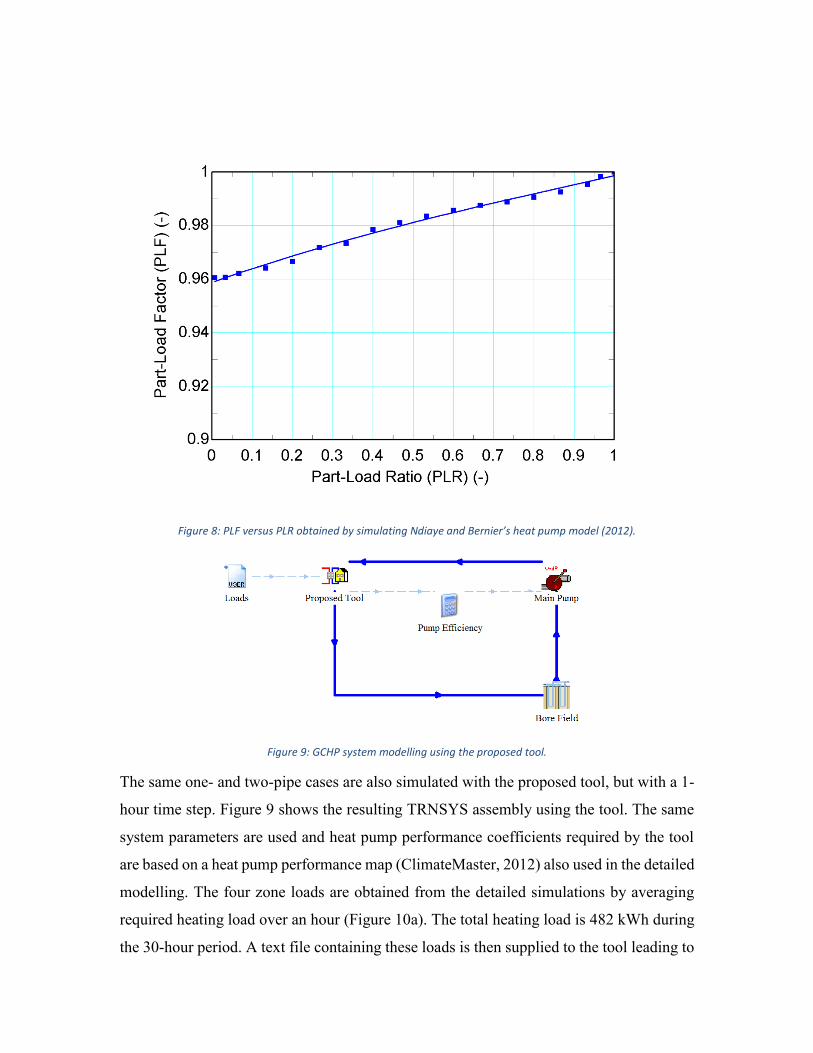
Figure 8: PLF versus PLR obtained by simulating Ndiaye and Bernier’s heat pump model (2012).

Figure 9: GCHP system modelling using the proposed tool.

The same one- and two-pipe cases are also simulated with the proposed tool, but with a 1-

hour time step. Figure 9 shows the resulting TRNSYS assembly using the tool. The same

system parameters are used and heat pump performance coefficients required by the tool

are based on a heat pump performance map (ClimateMaster, 2012) also used in the detailed

modelling. The four zone loads are obtained from the detailed simulations by averaging

required heating load over an hour (Figure 10a). The total heating load is 482 kWh during

the 30-hour period. A text file containing these loads is then supplied to the tool leading to

simulation results presented in Figures 10 and 11. As it can be observed, the same general

tendencies observed with the detailed simulation (hourly averages – Avg curves) are

predicted by the tool. One can note that the outlet temperature (inlet to the bore field) is

lower in the one-pipe network as the flow rate is generally lower in the proposed tool. In

terms of energy consumption, the tool predicts a total heat pump energy consumption of

134 kWh for the one-pipe and of 127 kWh for the two-pipe systems. The detailed

simulations predict corresponding energy consumption of 136 and 128 kWh, representing

less than a 1.5% difference. From this comparison, it can be concluded that the proposed

tool is in very good agreement with detailed simulations.

Figure 10a and b: Simulated power (top) and temperature (bottom) using the tool and a detailed modelling (One-pipe).

Figure 11a and b: Simulated power (top) and temperature (bottom) using the tool and a detailed modelling (Two-pipe).

The proposed tool was also used to find the best ∆T value for flow control in one-pipe

systems (see Figure 3b). Several test cases were evaluated all giving similar results. As

shown in Figure 12 for one of these cases (corresponding to Case 1 in the following

section), increasing the ∆T increases the main pump energy consumption as higher flows

are more often required. However, it also reduces heat pump energy consumption as higher

flows lead to more favorable bore field return temperature and less temperature changes

between heat pumps. The minimum total energy consumption for all studied cases,

including the one shown in Figure 12, is obtained for a ∆T between 5.5 and 6.5 °C.

Therefore, it is recommended to use a mean ∆T value of 6 °C (11 °F) when using one-pipe

systems.

Figure 12: ∆T optimization for the proposed one-pipe VFD control.

Case studies

This section demonstrates how the proposed TRNSYS tool can be used to compare one-

or two-pipe networks when designing a GCHP system. Four different cases are studied,

addressing two building geometries and two load profiles with ten 3-ton heat pumps in

each case. The first building, representing a 60×60 m (197×197 ft) square building with a

loop of four core and six perimeter heat pumps, is portrayed in Figure 5. The second

building is a 10×90 m (33×295 ft) longitudinal building represented by Figure 13. Both

buildings are one-story offices. The two load profiles are given in Figures 14a and 14b,

showing total heating and cooling loads over a year (cooling and heating can occur

simultaneously). The first one is a mixed load profile obtained using the climate of

Montreal (Canada) with an annual heating load of 101 800 kWh and an annual cooling load

of 110 100 kWh. The second load profile is a cooling-only load profile obtained using the

Miami (Florida) climate with an annual cooling requirement of 214 300 kWh. This is a

severe load for a GCHP system and a hybrid approach or large borehole separation might

be required in practice to avoid excessively hot return temperatures from the bore field

after a few years of operation. Since the following analysis examines only the first year of

operation, return temperatures are not excessive and heat pump performance degradation

is minimal.

Each system is coupled to a bore field composed of 10 boreholes. In all cases, borehole

length is selected such that the lowest or highest bore field return temperatures over the

year reach 0 °C (32 °F) or 35 °C (95 °F), which are the heat pump operating limits used in

these cases.

Figure 13: Second building heat pump position (Longitudinal).

Figure 14a and b: Mixed (left) and cooling-only (right) building load profiles over a year.

Loads are supplied to the tool which is coupled to a main pump and to a borehole model

(Figure 9). The main parameters used are presented in Table 2. The bore field model of

Godefroy and Bernier (2014) described earlier is also used in these case studies.

HP3

Mech. Room

HP2 HP4HP1

(20,10)(0,10)

(0,0)

(90,10)

HP9HP8HP7HP5

(40,10)

HP6

(30,10)(10,10) (80,10)(70,10)(60,10)

HP10

(50,10)

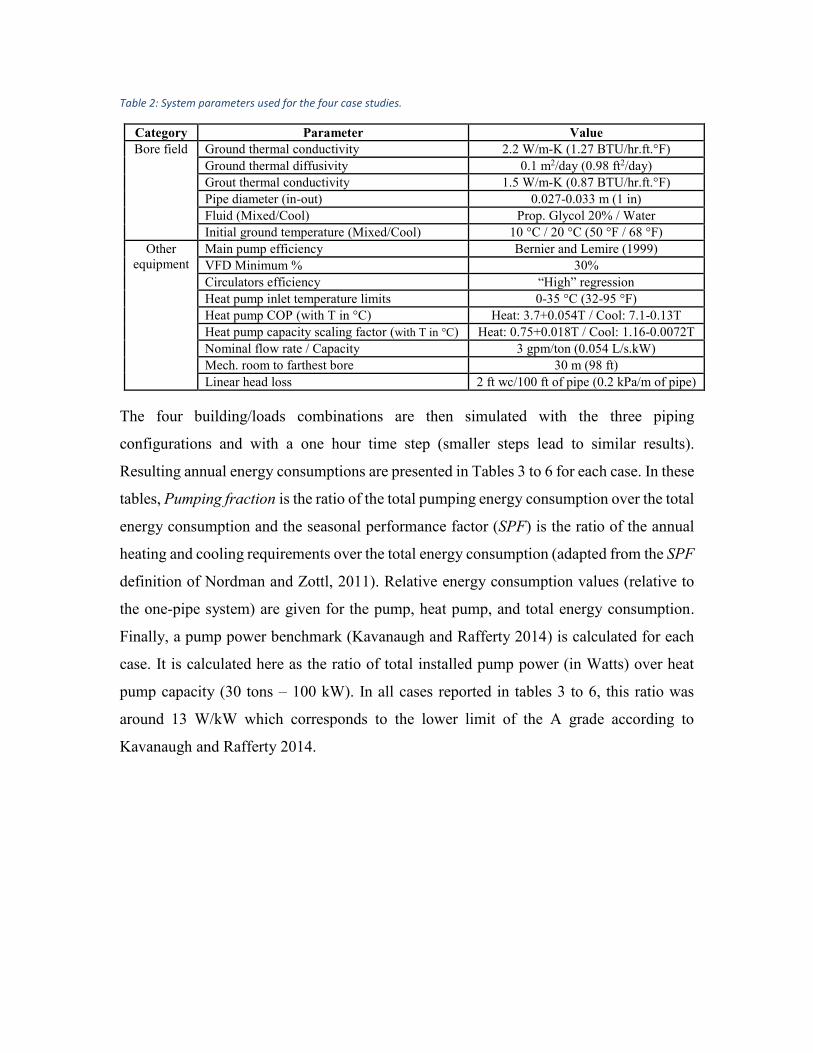
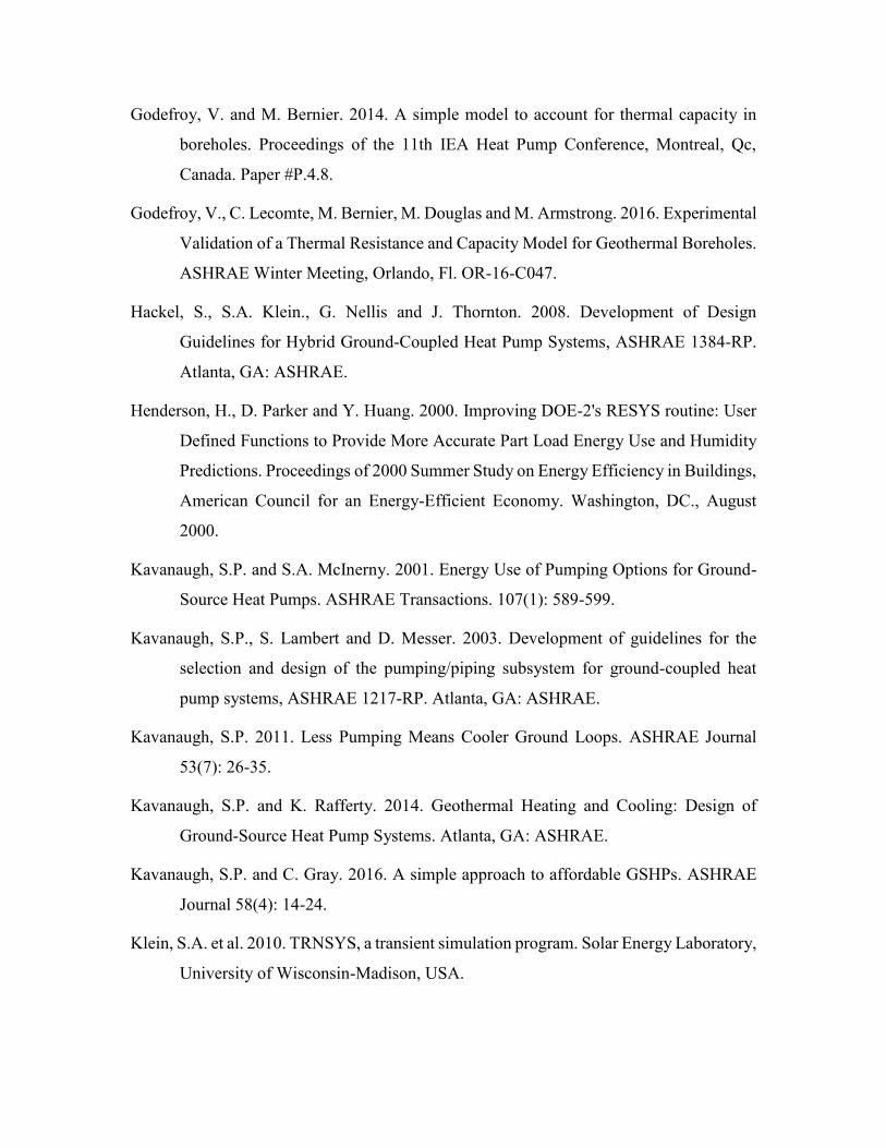
Table 2: System parameters used for the four case studies.

Category Parameter Value Bore field Ground thermal conductivity 2.2 W/m-K (1.27 BTU/hr.ft.°F)

Ground thermal diffusivity 0.1 m2/day (0.98 ft2/day) Grout thermal conductivity 1.5 W/m-K (0.87 BTU/hr.ft.°F) Pipe diameter (in-out) 0.027-0.033 m (1 in) Fluid (Mixed/Cool) Prop. Glycol 20% / Water Initial ground temperature (Mixed/Cool) 10 °C / 20 °C (50 °F / 68 °F)

Other equipment

Main pump efficiency Bernier and Lemire (1999) VFD Minimum % 30% Circulators efficiency “High” regression Heat pump inlet temperature limits 0-35 °C (32-95 °F) Heat pump COP (with T in °C) Heat: 3.7+0.054T / Cool: 7.1-0.13T Heat pump capacity scaling factor (with T in °C) Heat: 0.75+0.018T / Cool: 1.16-0.0072T Nominal flow rate / Capacity 3 gpm/ton (0.054 L/s.kW) Mech. room to farthest bore 30 m (98 ft) Linear head loss 2 ft wc/100 ft of pipe (0.2 kPa/m of pipe)

The four building/loads combinations are then simulated with the three piping

configurations and with a one hour time step (smaller steps lead to similar results).

Resulting annual energy consumptions are presented in Tables 3 to 6 for each case. In these

tables, Pumping fraction is the ratio of the total pumping energy consumption over the total

energy consumption and the seasonal performance factor (SPF) is the ratio of the annual

heating and cooling requirements over the total energy consumption (adapted from the SPF

definition of Nordman and Zottl, 2011). Relative energy consumption values (relative to

the one-pipe system) are given for the pump, heat pump, and total energy consumption.

Finally, a pump power benchmark (Kavanaugh and Rafferty 2014) is calculated for each

case. It is calculated here as the ratio of total installed pump power (in Watts) over heat

pump capacity (30 tons – 100 kW). In all cases reported in tables 3 to 6, this ratio was

around 13 W/kW which corresponds to the lower limit of the A grade according to

Kavanaugh and Rafferty 2014.

Table 3: Case 1 (Square/Mixed) - Simulation results for the 3 configurations.

Case 1 (Square/Mixed) One-pipe Two-pipe reverse-

return Two-pipe direct-

return

Total energy (kWh) (relative values)

56 339 (1.0)

54 861 (0.97)

55 912 (0.99)

Heat pumps energy (kWh) (relative values)

53 287 (1.0)

51 804 (0.97)

51 828 (0.97)

Main pump energy (kWh) 1 130 2 502 3 536 Circulators energy (kWh) 1 206 (-) (-) Total pump+circ (kWh) (relative values)

2 336 (1.0)

2 502 (1.07)

3 536 (1.51)

Pumping fraction (%) 4.1 4.6 6.3 SPF (-) 3.76 3.86 3.79 Main pump max ∆p (kPa/ft) 112/37 160/54 226/76 Circulators max ∆p (kPa/ft) 48/16 (-) (-) Interior piping (m/ft) 258/846 487/1598 487/1598 Borehole length (m/ft) 126/413 127/417 127/417

Table 4: Case 2 (Square/Cooling) - Simulation results for the 3 configurations.

Case 2 (Square/Cooling) One-pipe Two-pipe reverse-


return


73 583 (1.0)

69 778 (0.95)

70 915 (0.96)


71 115 (1.0)

67 100 (0.94)

67 209 (0.95)


2 428 (1.0)

2 678 (1.10)

3 706 (1.53)


Table 5: Case 3 (Longitudinal/Mixed) - Simulation results for the 3 configurations.

Case 3 (Longitudinal /Mixed) One-pipe Two-pipe reverse-


return


56 230 (1.0)

54 598 (0.97)

54 986 (0.98)


53 285 (1.0)

51 739 (0.97)

51 747 (0.97)


2 229 (1.0)

2 313 (1.04)

2 696 (1.21)


Table 6: Case 4 (Longitudinal/Cooling) - Simulation results for the 3 configurations.

Case 4 (Longitudinal /Cooling) One-pipe Two-pipe reverse-


return


73 432 (1.0)

69 724 (0.95)

70 156 (0.96)


71 104 (1.0)

67 236 (0.95)

67 283 (0.95)


2 328 (1.0)

2 488 (1.07)

2 874 (1.23)


Analysis and discussion

First, results show that one-pipe systems have a slightly higher (1 to 5%) total energy

consumption than two-pipe systems which leads to slightly lower 𝑆𝑃𝐹. Two-pipe systems

have a higher pumping energy consumption (4 to 53% higher than one-pipe system) but in

all cases the Pumping fraction is relatively small and varies from 3.2 to 6.3%. However,

heat pump energy consumption is 3 to 6% higher for one-pipe networks. The one-pipe

main flow rate is generally lower than in two-pipe systems, decreasing pumping

requirements but also main pump efficiency which reduces pumping energy savings over

two-pipe systems. It is also interesting to note that the sum of the head losses for the one-

pipe main pump and circulator is approximately equal to the reverse-return main pump

head loss. This is due to similar hydraulic path lengths and valve pressure drops. Direct-

return systems require more pumping energy than reverse return systems, leading to a

slightly higher total energy consumption.

The cooling-only cases present a higher energy consumption difference between

configurations. One-pipe network heat pumps experience an increasing inlet temperature

along the loop as all units are in cooling. Consequently, this increases heat pump and total

energy consumption of one-pipe networks.

Simulations using the proposed tool also show that choosing between a one- or two-pipe

network has only a small influence on the required bore field length. Heat pump COP and

pumping are influenced by the configuration, but not enough to significantly modify

ground loads. For a mixed load profile, one-pipe configurations lead to a 1 or 2 m length

reduction. This is due to the temperature drop along the primary pipe which reduces heating

COP and consequently the ground loads. However, for the cooling-only cases, deeper

boreholes are required for one-pipe systems as heat pump COP decreases along the loop

leading to more compressor power which is ultimately rejected into the ground.

It also appears that building geometry has only a small impact on energy consumption in

these cases. However, the geometry would probably have a more significant impact on

piping costs.

The main objective is to develop a versatile simulation tool in which users can set several

parameters. The studied cases were simulated to show how the proposed tool can be used

and the conclusions cannot be generalised with only four cases. Pumping energy results

are somewhat sensitive to the pressure drop of the connecting hoses and valves at the heat

pump. For example, if the 𝐶𝑣 of the control valve is reduced from 25 to 3.5, pumping energy

increases by about 20% in two-pipe systems. However, this increases total energy

consumption by only 1%.

Also critical is the selection of the nominal flow rate and pipe head loss. The previous cases

were calculated with typical conditions: flow rate of 3 gpm/ton and pipe head loss of 2 ft

wc /100 ft of pipe. Two parametric studies are performed with other nominal flow rates

and pipe head losses. The results are presented in Figures 15 and 16 based on Case 1

(Square building/Mixed loads). The total annual energy consumption is shown on the left

scale while relative values (compared to the reference one-pipe system) are shown on the

right axis. Figure 15 presents the effect of a variation of the nominal pipe head losses from

1 to 5 ft wc/100 ft of pipe for the three networks. It is shown that two-pipe networks are

more influenced by this parameter as the curves are steeper, which is mostly due to longer

interior pipes. It is the main pump energy consumption which increases as heat pumps and

circulators have similar energy consumption. It is also interesting to note that the one-pipe

network uses less energy than the direct-return case for pressure drops higher than 3 ft wc

/100 ft of pipe. This illustrates that the increase in pumping energy of two-pipe networks

can exceed the increase in heat pump energy consumption of one-pipe networks.

Thi study only examined operating energy costs for the first year. A life cycle cost study

where the lower first cost of one-pipe systems

Figure 15: Annual energy consumption influenced by pipe pressure drop (Case 1).

Figure 16 presents the effect of different nominal heat pump flow rates for the three

networks. For two-pipe systems, heat pump energy consumption is similar while pumping

energy increases with higher flows, leading to a total energy consumption increase. For

one-pipe systems, total energy consumption decreases when the nominal flow rate

increases from 1.5 to 2.25 gpm/ton and then increases when using 3 gpm/ton. As the flow

is increased from 1.5 to 2.25 gpm/ton, pumping energy increases but heat pump energy

consumption decreases even more as the loop temperature is less influenced by the

operation of preceding heat pumps. However, as the flow is increased from 2.25 to 3.0

gpm/ton, the pumping energy increase is greater than the drop in heat pump energy

consumption.

Figure 16: Annual energy consumption influenced by nominal flow rate (Case 1).

Conclusion

Several interior piping configurations are available for designers of centralized GCHP

systems. Two-pipe networks, either in reverse or direct-return, are common. However, they

require more piping and pumping energy than one-pipe networks which are simpler to

design but have a higher heat pump energy consumption. This paper proposes a simulation

tool to compare the energy consumption (pump and heat pump) of these configurations. A

flow control method for one-pipe systems, based on the bore field return temperature, is

also proposed. Four case studies are presented to show the usefulness of the tool with

typical conditions of flow rate (3 gpm/ton) and pipe head loss (2 ft wc /100 ft of pipe).

Results show that one-pipe systems have a slightly higher (1 to 5%) total energy

consumption than two-pipe systems. Two-pipe systems have a higher (4 to 53%) pumping

energy consumption than one-pipe systems. However, heat pump energy consumption is 3

to 6% higher for one-pipe networks.

Results are somewhat sensitive to the pressure drops in connecting hoses/valves at the heat

pump. For example, if the 𝐶𝑣 of the control valve is reduced from 25 to 3.5, pumping energy

increases by about 20% in two-pipe systems.

Parametric studies on the flow rate and nominal linear pipe pressure drop are also reported.

For one-pipe systems, total energy consumption decreases when the nominal flow rate

increases from 1.5 to 2.25 gpm/ton and then increases when using 3 gpm/ton. For two-pipe

systems, heat pump energy consumption is similar while pumping energy increases with

higher flows, leading to a total energy consumption increase. The nominal pipe head losses

is varied from 1 to 5 ft wc/100 ft of pipe for the three networks. It is shown that two-pipe

networks are more influenced by this parameter as the energy consumption curves are

steeper, which is mostly due to longer interior pipes. Finally, results also show that the

piping configuration has a relatively small influence on the overall length of the bore field.

A future study will address the piping cost difference between one- and two-pipe networks

and how it influences life cycle costs for such systems.

Acknowledgments

The authors would like to express their sincere gratitude to ASHRAE, Hydro-Quebec and

the Natural Sciences and Engineering Research Council of Canada (NSERC) who provided

scholarships to the first author. This work was also performed with funds provided by

NSERC’s Smart Net-Zero Energy Buildings Strategic Research Network.

Appendix A – Tool parameter, input and output description

Table 7 describes the parameters, inputs and outputs used in the proposed tool and

presented in Figure 4.

Table 7: Tool parameter, input and output description. Parameters

Type of Network Piping configuration among one-pipe, two-pipe reverse-return and two-pipe direct-return.

NB of HP Number of heat pumps to be simulated.

Pipe Linear Head Loss Nominal linear pressure drop in main pipes and bores, based on the maximum designed flow in each pipe segment.

HP COP Coefficients 4 coefficients for the constant and variable terms of the heating and cooling COP linear regressions, which are function of the unit inlet temperature.

HP Capacity Scaling Factors

4 coefficients for the heating and cooling capacity scaling factor linear regressions, which are function of the unit inlet temperature.

Circulator Efficiency Choice between 3 efficiency classes based on manufacturers data. Each class has a regression predicting efficiency as a function of the hydraulic power.

VFD Minimum % Minimum fraction reached by the VFD. Represents the lowest achievable maximum flow fraction.

Borehole length Length of the longer and farthest borehole from the mechanical room. Used to evaluate the worst hydraulic path.

L to Farthest Borehole Distance between the mechanical room (0,0) and the farthest borehole. Used to calculate the pressure drop in this segment.

T to HP Min Heat pump inlet temperature minimum operating limit. Used to set the one-pipe main flow rate.

T to HP Max Heat pump inlet temperature maximum operating limit. Used to set the one-pipe main flow rate.

∆T (One Pipe VFD) Temperature difference used to set the one-pipe main flow rate and over which the flow varies linearly.

Valve and hose Cv 5 valves/hose flow coefficients selected for a 3-ton heat pump using 3 gpm/ton. Used to evaluate pressure drop in each component.

PLF Coefficients 4 coefficients used to calculate the part-load factor based on heat pumps Part-Load Ratio. Set the first one (a0) to 1 to neglect PLF effects.

Nominal Capacity (i) Nominal capacity of heat pump (i) in tons. Used to determine heat pump nominal flow by multiplying the gpm/ton. This capacity is corrected depending on unit inlet temperature to evaluate the part-load operation.

Nominal GPM/Ton (i) Nominal flow rate of heat pump (i) in gpm/ton. This flow, typically 1.5 or 3 gpm/ton, influences pressure drop in valves, heat pumps and pipes.

X Position (i) X axis position of heat pump (i). Y Position (i) Y axis position of heat pump (i).

Inputs

T to HP Fluid temperature exiting the main pump (after the bore field) and entering in the first heat pump of the building (all heat pumps in two-pipe networks).

Fluid Cp Fluid thermal capacity. As an input, it can vary over time or be fixed. Fluid Density Fluid density. As an input, it can vary over time or be fixed.

Load (i) Heat pump load to be met during a time step. The selected convention states that a heating load is positive while cooling loads are negative.

Outputs

T to Bore Field Fluid temperature exiting all the heat pumps and entering in the bore field. It is calculated differently for one- and two-pipe systems.

Power HP Sum of heat pump power consumption accounting for varying COP, capacity and PLR.

Power Circulators Sum of circulator pump power.

Power Auxiliary Sum of all electrical auxiliary power (heating). % HP in Operation Fraction of heat pumps having a load ≠ 0.

Loop Load Sum of power exchanged with main loop by each heat pump (ground load). Heating Load Sum of the zone loads in heating. Cooling Load Sum of the zone loads in cooling.

Main Flow Flow that the main pump must provide. It is a function of the heat pumps in operation (two-pipe) or bore field return temperature (one-pipe). The maximum main flow is the sum of each heat pump nominal flow rate.

∆p Main Pump Overall pressure drop provided to the main pump. Only pipes and boreholes are considered for one-pipe systems.

Pump Correction Factor

Overall Part-Load Ratio of all operating heat pumps. Used to correct main pump power for flow variations over a time step.

∆pmax Circulators Maximum pressure drop experienced by circulators (one-pipe). Interior Piping Length Interior length of the main pipes to buy and install.

Nomenclature

∆p = Pressure drop (kPa) ∆T = Temperature difference (°C) η = Efficiency (%) Avg = Average CAP = Heat pump capacity (tons or kW) COP = Coefficient of performance (-) CR = Capacity ratio (-) CSF = Capacity scaling factor (-) Cv = Flow coefficient (gpm or L/s) D = Pipe diameter (m or in) EIR = Energy input ratio (-) f = VFD flow fraction (-) Fpump = Main pump correction factor (-) H = Pump head (kPa) Inst = Instantaneous L = Pipe length (m)

�̇� = Main flow rate (L/s)

�̇�𝑖 = Heat pump branch flow rate (L/s)

�̇�𝑡𝑜𝑡 = Maximum main flow rate (L/s) Mech. = Mechanical

PLF = Part-load factor (-) PLR = Part-load ratio (-) QLoop = Loop heat injection/rejection (kW) SPF = Seasonal performance factor (-) T = Temperature (°C) TRCM = Thermal resistance and capacity model VFD = Variable frequency drive W = Power (kW) X = Position relative to the X axis (m) Y = Position relative to the Y axis (m)

Subscripts

1pipe = One-pipe network 2pipe = Two-pipe network 1...14 = Index relative to Figure 1 Circ = Circulator corr = Corrected HP = Heat pump i = Specific to a heat pump linear = Relative to a specific pipe length min = Minimum max = Maximum nom = Nominal rev = Reverse-return s = Segment toHP = Heat pump primary loop entrance/after main pump

References

Bernier, M. and N. Lemire. 1999. Non-Dimensional Pumping Power Curves for Water

Loop Heat Pump Systems. ASHRAE Transactions. 105(2): 1226-1232.

Bernier, M., A. Sfeir, T. Million and A. Joly. 2005. A methodology to evaluate pumping

enegy consumption in GCHP systems. ASHRAE Transactions. 111(1): 714-729.

Bidstrup, N. 2012. EU Pump Regulations. ASHRAE Journal 54(5): 106-110.

Boldt, J. and J. Keen. 2015. Hydronics 101. ASHRAE Journal 57(5).

Cimmino, M. and M. Bernier. 2013. Preprocessor for the generation of g-functions used in

the simulation of geothermal systems. 13th Conference of International Building

Performance Simulation Association (IBPSA), p. 2675-2682.

Cimmino, M. and M. Bernier. 2014. A semi-analytical method to generate g-functions for

geothermal bore fields. International Journal of Heat and Mass Transfer, 70, p. 641-

650.

ClimateMaster. 2012. Tranquility 27 (TT) Series Performance Map. USA: ClimateMaster.

Cunniff, G. and B. Zerba. 2006. Single-Pipe Systems for Commercial Applications. HPAC

Engineering (October 2006), 42-46.

Cunniff, G. 2011. Less is more: single-pipe hydronic system solves high-rise troubles. PM

Engineer (September 2011), 18-22. 139

Duda, S.W. 2015. Reverse-Return Reexamined. ASHRAE Journal 57(8): 40-44.

Gagné-Boisvert, L. and M. Bernier. 2016. Accounting for Borehole Thermal Capacity

when Designing Vertical Geothermal Heat Exchangers. Presented at the 2016

ASHRAE Annual Conference, St-Louis, MO, June 25–29.

Gagné-Boisvert L. and M. Bernier. 2017. A comparison of the energy use for different heat

transfer fluids in geothermal systems. Proceedings of the 2017 IGSHPA Conference

and Expo, March 14-16 2017, Denver, USA, pp. 336-345.

Godefroy, V. and M. Bernier. 2014. A simple model to account for thermal capacity in

boreholes. Proceedings of the 11th IEA Heat Pump Conference, Montreal, Qc,

Canada. Paper #P.4.8.

Godefroy, V., C. Lecomte, M. Bernier, M. Douglas and M. Armstrong. 2016. Experimental

Validation of a Thermal Resistance and Capacity Model for Geothermal Boreholes.

ASHRAE Winter Meeting, Orlando, Fl. OR-16-C047.

Hackel, S., S.A. Klein., G. Nellis and J. Thornton. 2008. Development of Design

Guidelines for Hybrid Ground-Coupled Heat Pump Systems, ASHRAE 1384-RP.

Atlanta, GA: ASHRAE.

Henderson, H., D. Parker and Y. Huang. 2000. Improving DOE-2's RESYS routine: User

Defined Functions to Provide More Accurate Part Load Energy Use and Humidity

Predictions. Proceedings of 2000 Summer Study on Energy Efficiency in Buildings,

American Council for an Energy-Efficient Economy. Washington, DC., August

2000.

Kavanaugh, S.P. and S.A. McInerny. 2001. Energy Use of Pumping Options for Ground-

Source Heat Pumps. ASHRAE Transactions. 107(1): 589-599.

Kavanaugh, S.P., S. Lambert and D. Messer. 2003. Development of guidelines for the

selection and design of the pumping/piping subsystem for ground-coupled heat

pump systems, ASHRAE 1217-RP. Atlanta, GA: ASHRAE.

Kavanaugh, S.P. 2011. Less Pumping Means Cooler Ground Loops. ASHRAE Journal

53(7): 26-35.

Kavanaugh, S.P. and K. Rafferty. 2014. Geothermal Heating and Cooling: Design of

Ground-Source Heat Pump Systems. Atlanta, GA: ASHRAE.

Kavanaugh, S.P. and C. Gray. 2016. A simple approach to affordable GSHPs. ASHRAE

Journal 58(4): 14-24.

Klein, S.A. et al. 2010. TRNSYS, a transient simulation program. Solar Energy Laboratory,

University of Wisconsin-Madison, USA.

Mescher, K. 2009. One-Pipe Geothermal Design: Simplified GCHP System. ASHRAE

Journal 51(10): 24-40.

Ndiaye, D. and M. Bernier. 2012. Transient model of a geothermal heat pump in cycling

conditions – Part B: Experimental validation and results. International Journal of

Refrigeration 35(8):2124–2137.

Nordman, R. and A. Zottl. 2011. SEPEMO-Build - a European project on seasonal

performance factor and monitoring for heat pump systems in the building sector.

REHVA Journal 48(4): 56-61.

Salim Shirazi, A. and M. Bernier. 2013. Thermal capacity effects in borehole ground heat

exchangers, Energy and Buildings, 67:352-364.

Stethem, W.C. 1994. Single-pipe hydronic systems – Design and load-matched pumping.

ASHRAE Transactions. 100(1): 1507-1515.

Stethem, W.C. 1995. Single-pipe hydronic systems – Historical development. ASHRAE

Transactions. 101(1): 1251-1259.

Taylor, S. and J. Stein. 2002. Balancing variable flow hydronic systems. ASHRAE Journal

44(10).

Documents

Titre: Integrated model for comparison of one-and two-pipe