PLANE WAVE SYNTHESIS : A NEW APPROACHTO THE PROBLEM OF ANTENNA

NEAR-FIELD/FAR-FIELD TRANSFORMATION

by

E. P. Schoessow, B.Eng.

A thesis presented in candidature forthe degree of Doctor of Philosophy,University of Sheffield, Department ofElectronic and Electrical Engineering.

September 1980.

To my Parents

SUMMARY

In the recently evolved fields of satellite and

space communications as well as in a number of related

areas, a vital requirement is an accurate knowledge of

the radia'ting and receiving characteristics of the trans-

mitting and receiving antennas as they appear at a large

distance (in the so called far-field region). It is often

impossible to obtain a direct measurement of the performance

of an antenna and in such cases where it is possible, the

accuracy obtainable is frequently limited by the many

difficulties associated with the process.

Over recent years, a number of techniques have begun

to appear which allow measurement of data close to the test

antenna (in the near-field region) and then by mathematical

processing (the transformation) predict what the far-field

performance will be. The earlier techniques while being

basically simple from a mathematical viewpoint, were not

completely general and tended to involve special, sophis-

ticated, hardware. The later techniques use the most

general spherical scanning system but involve much more

complicated processing.

A new approach to the problem is presented in which

much of the computational burden is pre-processed so thatthe size and complexity of the ultimate prediction task is

reduced. The various measurement systems are considered

briefly and the spherical system is formulated in detail.

Simulated and experimental predictions are carried out

and studies are included of the vario~s errors likely to

be present and their effects. The important parameters,

including the sampling criterion, are discussed in some

detail.

It is shown that this technique has the potential

for producing rapid and accurate predictions of antenna

far-field patterns including the facility of compensation

for the characteristics of the measurement probe.

PUBLICATIONS

Parts of the work described in this thesis have

formed the basis of a number of publications. These are:

Bennett, J.C. and Schoessow, E.P., 'Near-fie1d/far-field transformation using a plane wavesynthesis technique', 3rd Antenna Symposium,Queen Mary College, London, 1977.

Bennett, J.C. and Schoessow, E.P., 'Near-fie1d/far-field transformation using a plane wavesynthesis technique', Proc., Workshop on antennatesting techniques, ESTEC, Noordwijk, Netherlands,1977, pp.135-136.

Bennett, J.C. and Schoessow, E.P., 'Near-fie1d/far-field transformation using a plane wavesynthesis technique', Proc.IEE, 125, 1978,pp.179-184. -

Schoessow, E.P. and Bennett, J.C., 'Recent progressin the plane wave synthesis technique for antennanear-field/far-field transformation', Proc.lnter-national Conference on Antennas and Propagation,lEE, London, 1978, pp.123-127.

Bennett, J.C. and Schoessow, E.P., 'Near-field tofar-field transformation using a plane wave synthesistechnique', Proc.seminar on Compact Antenna Ranges,Royal Signals and Radar Establishment, Malvern, 1980.

ACKNOWLEDGEMENTS

The author wishes to express his appreciation to a

number of individuals and organisations whose help has

been of great value to the work described in this thesis:

- Professor F.A. Benson and the University of Sheffield,

Department of Electronic and Electrical Engineering

for the facilities made available during the work.

- Dr. J.C. Bennett and Dr. A.J.T. Whitaker both of whom

have made invaluable practical contributions to the

work and always made themselves available for

discussions when requested.

- The many other members of the Department of Electronic

and Electrical Engineering who have made contributions

to the progress including David Cox (the test site

technician) and Haydn Flower and his workshop staff.

- Mr. K. Kilford and the Department of Civil and

Structural Engineering for the temporary loan of a

sensitive optical level.

- The U.K. Science Research Council and latterly the

Ministry of Defence for financial support.

- Margaret Eddell for kindly offering her services as

typist for this thesis.

e, <P

ew, <PweF, <PF

ep, <Pp

x, y, z

Xp, yp' Zp -

Ak = 27T/Ar

R

D

g(e,<p)

em' <Pmp(eF,<PF)

rpw, epw

Ex

-i-

LIST OF PRINCIPAL SYMBOLS

spherical coordinates, particularly in near-field data.

spherical coordinates in weighting function.

far-field spherical coordinates.

spherical coordinates in probe measurementsystem.

general Cartesian coordinate.

Cartesian coordinates of probe.

wavelength.

propagation ( phase) constant.

general distance.

radius of near-field measurement sphere.

diameter of synthesised plane wave.

weighting function.

limits of g(e, <P).

predicted far-field at(eF, <PF)

polar coordinates of point in plane wave.

electric field component in x-direction(other directions denoted with differentsubscripts) •

-ii-

CONTENTSPage No.

1. INTRODUCTION1.1 Background to the Subject

.1.2 Far-Field Simulation Techniques

1

14

1.2.1 Antenna Refocussing1.2.2 The Compact Range

44

1.3 Near-Field/Far-Field Transformation 51.3.1 Fourier Transformation based upon

the Scalar Diffraction Formula 61.3.2 Planar Scanning 71.3.3 Cylindrical Scanning 91.3.4 Spherical Scanning 9

1.4 The Objectives of the Present Work 111.5 The Spherical Scan Geometry 12

1.5.1 Elevation-Over-Azimuth System1.5.2 Polarisation-Over-Azimuth System

1.6 Phase Convention1.7 Simulation Program PCMPID

2. THE PLANE WAVE SYNTHESIS TECHNIQUE

12131415

2.2.12.2.22.2.3

Generation of \veightingFunctionDepth of Field and Limits of g{6,¢)Basic Prediction Process

171720202132344041

2.12.2

The Basic ConceptInitial Scalar Approach

2.32.42.5

Sampling CriterionVisualisation of Field DistributionsTwo-Dimensional Experimental Results2.5.1 Conclusions from the Two-

Dimensional Results 453. THREE-DIMENSIONAL PREDICTION WITH PROBE

COMPENSATION USING AN ELEVATION-OVER-AZIMUTH SCANNING GE01-lliTRY3.1 The Approach Used

3.1.1 Rotation 13.1.2 Rotation 23.1.3 Resulting Field Components

3.2 Introduction of z-Offset3.2.1 Resulting Field Components

4646

484950

5253

3.3 The Iteration Procedure 543.4 Typical Parameters for the Weighting Function 56

-iii-

Pase No.3.5 Three-Dimensional Scanning 58

3.5.1 Prediction of ESF for ¢F =I 0 593.5.2 Prediction of E<j>F 60

3.6 The Composite ~JeiightingFunction 613.7 Interpolation Schemes 64

4. THREE-DI~mNSIONAL PREDICTION WITH PROBECOMPENSATION USING A POLARISATION-OVER-AZIMUTH SCANNING DEVICE4.1 The Coefficients

4.1.1 Field Components4.2 z-Offset4.3 The Iteration Procedure

4.3.1 Timing Difficulties

686970717273

4.4 Application of an Elevation-Over-AzimuthWeighting Function 734.4.1 Prediction of E¢F 744.4.2 Prediction of ESF 76

5. PROBE COMPENSATION EFFECTS AND ERROR ANALYSIS 785.1 Probe Compensation 78

5.1.1 Effects upon the Synthesised Plane Wave 795.1.2 Fourier Transform Analysis 805.1.3 A Simulation 84

5.2 Effects of Measurement Errors 855.2.1 Level-Independent Random Noise5.2.2 Non-Ideal Probe5.2.3 Other Measurement Errors5.2.4 Mechanical Errors

5.3 Weighting Function Edge Effects5.4 Frequency Tolerance of the Weighting5.5 Range/Wavelength Scaling

6. THREE-DIMENSIONAL VERIFICATION6.1 Antenna Test Range and Equipment6.2 System Alignment

6.2.1 The Alignment Procedure6.2.2 The Test Antenna

6.3 The Scans Performed6.4 Far-Field Predictions6.5 Pattern Discrepancies

8587878991

Function 93949696

100101105106109111

-iv-

Page No.7. CONCLUSION 119

7.1' Summary of the Work to Date 1197.2 Application to Other Measurement Systems 1217.3 Type of Probe 1237.4 Processing Efficiency 1237.5 Efficient Weighting Function Generation 124

7.5.1 Small Antennas7.5.2 Large Antennas

7.6 The" Standard" Weighting Function7.7 Conclusions

124125126126

Appendix 1: IMPULSE RESPONSE OF THEWEIGHTING FUNCTION 127

Appendix 2: SAMPLING EFFECTS 130A2.l Far-Field Weighting Functions 130A2.2 Near-Field Weighting Functions 131

Appendix 3: ANGULAR EXTENT OF THEWEIGHTING FUNCTION 134

Appendix 4: THE V-72 IMAGE PROCESSING COMPUTER 136A4.l C.I.L Incremental Plotter 137A4.2 Mk 6 T.V. Display 137

Appendix 5: SOFTWARE WRITTEN FORPLANE WAVE SYNTHESIS 139

REFERENCES: 142

-1-

1. INTRODUCTION

1.1 Background to the Subject

In the very early days of radio communication, with

so much available space in the frequency spectrum,

multiple use of the same wavelength was largely unnecessary

and therefore the problems caused for the receiver operator

by interference from unwanted transmissions were slight.

As time progressed and the number of transmitting stations

increased, the phenomenon of multiple-source interference

became more apparent. Clearly partial solutions to the

problem were readily available:

(a) A limit could be imposed on the power to be radiated

from any particular transmitter. Space attenuation

could then be relied upon to reduce the unwanted

signal to acceptable levels.

(b) The receiver could be made more frequency-selective

so that transmissions on even very similar wave-

lengths could be adequately separated.

These are indeed two of the basic methods used for

avoiding interference as far as public broadcasting isconcerned. A few moments, however, spent listening to

the medium-wave A.M. broadcast band, for instance, areample demonstration that these techniques alone are, inmany circumstances, far from sufficient.

The other obvious remedial action was the use of areceiving antenna with particular, non-isotropic reception

characteristics {and in the case where a particular

transmitter-receiver link was involved, this was equally

-2-

applicable to the transmitting antenn~). Engineers

applied their talents, therefore, to the design of

suitable antennas.

Originally certain types of directive antennas

were constructed on an essentially empirical basis but

their performance still had to be evaluated. At the

frequencies then most used, this seldom presented serious

difficulty, since the far-field patterns of the antennas

were established at quite short ranges. This meant that

the radiation patterns could be measured directly. In any

case, the antennas were required usually for ground-to-

ground fixed station communication and therefore the ground

coverage could be (and indeed had to be) investigated insitu.

The situation is vastly different nowadays. With the

increasing use of higher frequencies and, in particular,

the associated progression in the electrical size of antennas

from a fraction of a wavelength to, in some cases, many

hundreds or even thousands of wavelengths, the distances

required to perform direct far-field measurements have

become impossibly large. In such applications as radio

astronomy and satellite and space communications, it is

almost invariably the far-field pattern which is of

importance and, in the latter instances, bearing in mind

the vast sums of money involved, it is essential that the

measurements should be carried out on Earth so that any

faults can be corrected before launch. At best, an incorrect

radiation pattern means that a satellite antenna, for instance,

may be wasteful of the precious power available. At worst,

-3-

for example where security is importan~, a high sidelobe

in the wrong place may mean that the device is useless.

In a deep space probe, where achieving the maximum

possible gain is vital, an antenna fault may mean total

failure of the mission.

Even when a direct measurement of a far-field

radiation pattern is possible, there are many problems

accompanying the use of long outdoor measurement

ranges:

(a) Range reflections.

(b) Atmospheric effects, dependence upon weather

conditions and lack of climatic control.

(c) The relatively high power requirement to achieve a

usable signal-to-noise ratio.

(d) Interference from unwanted signals.

(e) Interference created for other people.(f) Lack of security.

(g) Cost of real estate.

These mean that the order of accuracy now being sought

is often unattainable (or unaffordable). As a result,

other techniques for evaluating the performance of antennas

have been developed. These may be divided broadly into

two groups: those that attempt to simulate the far-field

measurement conditions in the near-field and those that

use numerical manipulation of measured near-field data to

predict the far-field pattern (the so called near-field/

far-field transformation).

-4-

1.2 Far-Field Simulation Techniques

1.2.1 Antenna RefocussingThis technique(!)(2) relies on the principle that,

"if the probe cannot be taken to the far-field, the far-

field must be brought to the probe". This is re~evant,

'in particular, to reflector antennas and uses the

property that if the feed position is suitably adjusted in

the axial direction, a pattern often quite similar to the

far-field pattern can be made to exist in the near-field.

This suffers from several serious drawbacks:

(a) Limited applicability. The method can only be

applied to certain reflector antennas.

(b) It requires the ability precisely to adjust (and

subsequently reset) the axial position of the feed.

(c) It is not totally accurate and gives particularly

poor results at large angles from boresight.

1.2.2 The Compact RangeThe compact range near-field technique is particularly

relevant to the main body of this thesis. It relies on the

fact that in the region a short distance in front of a

precisely made (and suitably fed) parabolic reflector antenna,

the field distribution is essentially that of a plane wave

(Fig. 1.1). Thus the plane wave response (which is identi-

cally the far-field response) can be measured for a test

antenna placed within that region. Various publications havedescribed compact ranges in more detail (3)(4)(5~ The main

disadvantages seem to be:

(a) The specialised hardware - the reflector.

planewave

compact rangereflector

test antenna

/....---- feed

Fig. 1.1. The compact range principle.

-5-

(b) The test antenna size is limited to being rather

smaller than the compact range reflector.

It has been proposed that a dielectric lens might

be used instead of the reflector (6). Similar drawbacks

to those above apply in this case.

Compact ranges have become established tools in

antenna measurement and quite a number are now in usethroughout the world.

1.3 Near-Field/Far-Field Transformation

In the near-field/far-field transformation, mathematical

processing of data acquired close to the antenna is employed

in an effort to predict what would be measured by an ideal

far-field test range. An ideal test range may be taken to

be one in which an infinitesimal probe, correctly polarised,

is placed a very large distance from the test antenna. Both

the antenna and the probe should be suspended in free-space

with no extraneous support or feed structures and remote

from any other bodies. The receiving system should be

totally noise-free and no other signal sources (whether

man-made or natural) should exist. This is not, of course,practically realisable.

The theory relating the fields existing near to an

antenna to those remote from it is far from simple and it has,

in general, been considered necessary to solve a substantial

number of field equations. Analytical solution of the

equations is usually either impossible or so tedious as to

be impracticable but with the rapidly increasing power of

modern computing equipment, numerical treatment has become

-6-

feasible. Even so, the complexity of hardware and

software requirements has meant that although the

theoretical basis for performing the near-field/far-field

transformation has been in existence for a few years, it

is only comparatively recently that operational ranges have

appeared (e.g. U.S. National Bureau of Standards, Georgia

Institute of Technology, Technical University of Denmark).

It may be useful, at this point, to review briefly some of

the existing techniques.

1.3.1 Fourier Transformation based uponthe Scalar Diffraction Formula

The Fourier transform relationship approximation

between the field distribution over a radiating aperture

and its far-field pattern is well known. It relies

essentially upon the Kirchoff scalar diffraction formula(7)

and has been investigated and exploited in various

h(8) (9) (10)sc emes . The process in a simplified form is as

follows. A two dimensional Fourier transform (normally

effected by means of a "fast Fourier transform" - FFT -

algorithm) is performed upon the measured near-field data

to yield (after some phase corrections and within the limits

of the paraxial approximations made) the field distribution

over the antenna aperture (or over an arbitrary plane passing

through or near the origin of the coordinate system).

Subsequent inverse transformation gives a prediction of the

far-field pattern. Unfortunately, because of the paraxial

approximations made, the technique is strictly only useful

for a very directive antenna and for the prediction of the

pattern near to boresight. Nevertheless, it is a tool which

-7-

can prove very useful if these limitations are

acceptable.

1.3.2 Planar Scanning

Another concept which has been utilised successfully

in antenna work is that of the infinite plane wave spectrum

of a radiated field. It can 'be shown(11) that the fields

radiated by an antenna can be rewritten as the sum of a series

of plane waves propagating in different directions. The

object of the technique, termed plane wave expansion, is to

determine the unknown amplitudes and phases of these

different plane waves obtaining what is known as a modal

expansion of the field. This is achieved using the measured

near-field over a planar surface (Fig. 1.2). The expansion

may then be extrapolated to the far-field to provide the

pattern prediction. The process is described in moredetail by Paris et al (12),Joy et al (13)and Joy and Paris (14)

(and also in a slightly modified approach by Kerns(1S) and it

is demonstrated that it becomes computationally efficient

since an FFT algorithm can be employed to perform the

numerical integrations involved.

Antenna pattern prediction utilising planar scanning

is possibly the most deeply investigated method and has been

shown to give good prediction accuracy. It has the advantage

(particularly as compared with spherical scanning methods)

of numerical simplicity and, because the scan is performed

by the probe, no positioning system is required for the testantenna. Under certain circumstances, this latter can prove

to be an advantage but at other times becomes a drawback:

test antenna

scan surfacey/x

z

Fig. 1.2. Planar scanning.

-8-

(a) The planar scanning system itself is a fairly

complicated device presenting probably more

mechanical problems than the more conventional

positioner systems. Therefore the capital cost

involved in actually setting up a measurement

facility could be greater.

(b) The size of antenna which can be accommodated is

limited by the size of the scanning device whereas

a spherical scanning method might be applicable even

to a very large antenna if it can be measured in situ

using its own positioner system.

The other chief disadvantage is that a set of measure-

ments can provide predictions over only a limited angular

range (as determined by the size of the scanning device and

in any event limited to less than the half-space behind the

scan plane). Another point particularly significant in this

scheme is the need to incorporate compensation for the

radiating characteristics of the near-field probe being used.

Because, in a spherical scanning technique, the probe always

points towards the origin of the coordinate system, the need

for compensation is not so vital if the probe is suitably

chosen since the variations in the illumination of the test

antenna will be small (although for maximum accuracy, the

possibility of including probe compensation is desirable).

This argument does not apply in the case of planar scanning

since, even with a small (and therefore wide-beam) probe,the test antenna can pass through an appreciably greater

angular range of the probe pattern to introduce large

variations in the illumination. This becomes even more

-9-

important when one realises that the requirement of

achieving the best signal-to-noise ratio in the measurements

tends to favour narrower beam probes.

1.3.3 Cylindrical Scanning

Here, the radiated fields are generally evaluated inthe form of a cylindrical wave expansion (16)(17)(although

the method devised by Borgiotti(1S) utilises a superposition

of plane waves) and again the problem reduces to that of

determining the various coefficients. Once more, computa-

tional efficiency is enhanced by the possibility of using

the FFT to perform the numerical integrations.

An advantage of the cylindrical scheme over the planar

one is that in one of the scan coordinates, prediction is

possible right around the antenna. Additionally, the

mechanical requirements are less severe since the probe

positioner is a simple linear device and the other scanning

coordinate is achieved by virtue of a conventional azimuth

positioner (Figures 1.3 and 1.4). A disadvantage is that

the numerical processing is a little more complicated.

Probe compensation is again important.

The cylindrical scanning approach has not been so

widely utilised as planar scanning but it has been demonstratedto be experimentally and computationally viable(l9).

1.3.4 Spherical Scanning

The major advantage of using a spherical surface is

that a single set of measurements can provide radiationpattern predictions over the full spherical far-field surface.

Additionally, as already mentioned, because of the nature of

testantenna

\probe

azimuth/ positioner

linearscanner/

Fig. 1.3. The cylindrical scan system.

>-

test antenna

scansurface

Fig. 1.4. The sample geometry produced by a cylindrical scan.

-10-

this scan geometry, probe compensation, is not so necessary

as in the other systems (although for maximum accuracy,

it should certainly be incorporated - Chapter 5 provides

information about the errors likely to be introduced by

incorrect probe compensation).

Conventionally, the spherical measurement geometry has

been regarded as presenting the greatest problems as regards

the necessary computing power. The near-fields are analysed

f h' 1 ' (20) (21) (22) whLehin the form 0 a sp erlca wave expanslon

can then be extrapolated to another measurement range, usually

the far-field. It has been found difficult to express the

formulae in such a way as to enable efficient computation

(such as the FFT) to be utilised for the numerical integra-

tions although recent work (23) has considerably improved the

efficiency. Nevertheless, the memory requirements are very

heavy, a figure of 1200 k words being quoted as the requirement

for processing a 10 x 10 data scan (equivalent to about 50 Ao 0antenna) with 90 k being needed even for a 30 x 30 set.

From the hardware point of view, spherical scanning is

possibly the most straightforward since a conventional dual-

positioner configuration (elevation-over-azimuth, azimuth-

over-elevation or polarisation-over-azimuth) is all that is

required. Furthermore there is effectively no limit on the

size of antenna which can be measured (at least as regardshardware) in contrast to the previous two schemes in which the

probe positioning systems provided a limit.

The limit on the size of antenna which can be measuredis provided by two factors; the time taken to acquire thedata (which can run into many hours) and the processing

-11-

requirements (in terms of time and o~ the amount of storage

needed). The constraint is thus on the electrical size

rather than the physical size of the test antenna and

figures quoted for maximum possible antenna size are

typically in the region of 100 A or less.

1.4 The Objectives of the Present Work

As has been seen, the least demanding computational

requirements for a near-field/far-field transformation

correspond to what is probably the least flexible and least

general scan geometry; planar. At the opposite end of the

scale, the most general and probably the easiest scanning

system to implement (spherical) requires the greatest

computing power. At the end of the present study, it would

be desirable to have a scheme which can utilise certainly

the spherical scan geometry (and ideally be applicable to

the others) but requires simpler processing. In particular,

the processing which takes place after the measurements have

been obtained should be kept to a minimum, i.e. as much of

the work as possible should be accomplished by preprocessing.Accuracy should, of course, be preserved.

The idea which emerged from this line of thought is

based on a concept similar to that described by Martsafey(24)

(although this publication came to light some considerabletime after the present approach evolved and some of the mainfeatures of the present method are given little or no

consideration). It is termed plane wave synthesis and

relies on the precomputation of a weighting function to be

applied to the measured data. The details of the technique

-12-

are given in later chapters. It is noted here that this

volume is devoted almost entirely to the implementation of

the technique in the spherical scan case, and we now

proceed to introduce the spherical scan geometry and the

conventions used.

1.5 The Spherical Scan GeometryOnly two forms of spherical scan geometry are used

in this thesis, elevation-over-azimuth and polarisation-

over-azimuth. The azimuth-over-elevation geometry can be

regarded as an elevation-over-azimuth system rotatedothrough 90 .

1.5.1 Elevation-Over-Azimuth System

In the elevation-over-azimuth scanning system, the

lower of the two positioners is an azimuth device with its

axis vertical. Mounted on this turntable is an elevation

positioner with its axis horizontal. The resulting

arrangement is such that a stationary probe covers an

effective measurement surface (when a test antenna is

scanned on the system) which is spherical (if the two

positioner axes intersect) and of the form shown in Fig.l.S

with the two poles of the scan geometry occurring at either

end of the elevation axis. The conventions used throughout

.this thesis as regards the Cartesian coordinates, x, y and

z, and the angular coordinates, e and ¢, are shown in Fig.

1.5 and also in more detail in Fig. 1.6. It may be worth

noting that these coordinates as used here do not necessarilycorrespond exactly with their usage elsewhere.

y

I I , ,'" - - - ,- , >

,,1),'1 I r- ... /

'''I " I~, >: '\.I, , -'i ....I- I - r .....,..... ' "" ,A } .....t' ,,~ .I"', "," '\

'\ ,t -I .... ' 1'-' ,,., \J. ,,\ - ;' 0(', \ \.) ....I , ....<troJ , '\ ,

, \ ' '" ' , , I I , .. " ~ " \ \ '"I I (" 1_ ,- _, , " ,,\

- __ --' \ '\, \. ,. I ...., .I > ' \, "'\I ": r: ,]I" " ",> < ". \ ,\' It " ' 'I I I I , .l '" r- ... )", ' \ _, T' I, > , Y ,I....l ? ..." ,A. \ \ , ~ < " , ' ..... " , ,. r....._ "'''''','1''''-, - \ _-,

I r-:'~ '''':::J~ --1- '_- r -~-" ,~.....- -,- - ~- 1, - l' - ", I I", ~'";..,':- - _ I J.

- \ ..". ..... .1 "...'.L' ",,' < " .! -;-,) .... ',1"' /..--_ I I ~

"" ,\ ,\" .... I -, - 7 -1."(' ..,.- I I '

, "\ ,"" ....v...... ' 7 _, J,.

\ '"" ..... , ;......... , '"""'" - ,-" ""'" ~ -....\ \- "

-,...

Fig. 1.5. The sample geometry produced by an elevation-over-azimuth spherical scan system.

y

point (e,~)

zFig. 1.6. Detail of the elevation-over-azimuth spherical

coordinates as used throughout this thesis.

· -13-

Two possibilities for the form qf the elevation

positioner exist: the side-pivoted and the rear-pivoted

(illustrated in Fig. 1.7). The rear-pivoted system is the

more popular since the mounting structure is more compact

and further from the front of the test antenna but it

suffers from the drawback that it cannot execute a full

spherical scan (since it cannot point directly downwards).

The side pivoted system has, in principle, the capability

for performing an all-space scan but has the disadvantage

of a more prominent (and therefore reflection-prone)

structure and furthermore, when the antenna is at -900

elevation (looking downwards) it is pointing directly atthe nearby support structure (and azimuth turntable) which

will cause quite serious reflection problems in many cases.The spherical positioning system which overcomes, to a

large extent, these difficulties is the polarisation-over-azimuth system which will now be described.

1.5.2 Polarisation-ever-Azimuth SystemBecause the polarisation-over-azimuth scan geometry

(illustrated in Fig. 1.8) is such that at no time does thetest antenna point towards the support structure, it suffers

rather less from problems of reflection. It still provides,however, the capability for an all-space scan. A minor

drawback is that with a single-polarisation probe only one

principal plane cut can be made with co-polarisation, all

the other possible cuts being at various other polarisations.

An elevation-over-azimuth system can produce co-polar

motor, gears etc..test antenna

~ azimuth positioner

Ca) Side-pivoted

Cb) Rear-pivoted test antenna

elevationpositioner

- azimuth-positioner

Fig. 1.7. Types of elevation positioner

polarisation positioner

/ test antenna

probe

positionertower

azimuthpositioner

)>--

f

Fig. 1.8. The polarisation-over-azimuth spherical scan system.

-14-

pattern cuts along both principal planes and indeed,

if Ludwig's second definition (25) of polarisation (rotated

through 900) is used, along any other cut also. The

equivalent can only be done on a polarisation-over-azimuth

system if a dual polarised probe is used and then only by

Gombining the two polarisations of data correctly. Since,

however, any practical spherical near-field measurement

system is likely to incorporate a dual-polarised probe,

the disadvantage is very slight. It may be worth noting

here, that if the probe is also mounted on a polarisation

turntable, then cuts of polarisation in accordance with

Ludwig's third definition (25) can be measured simply.

The spherical measurement surface produced by a

polarisation-over-azimuth scan system together with the

coordinates x, y, z, e and et> used as the convention through-

out the thesis, for this geometry, are illustrated in

Fig. 1.9 and the coordinate system in greater detail in

Fig. 1.10.

1.6 Phase ConventionFirstly it should be mentioned that, in the usual

way, where field quantities are referred to in the text,

the factor exp jwt, embodying the sinusoidal time variation,

is assumed. The second point is that throughout the thesis

the convention is employed that leading phase is to be

regarded as positive so that for radiation from a particular

point, for instance, the phase variation at any particular

moment in time will become increasingly negative with

increasing distance (i.e. of the form exp - jkr where

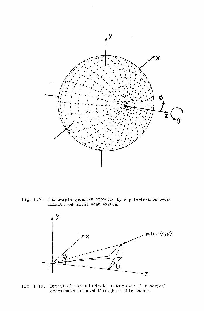
Fig. 1.9.

Fig. 1.10.

..

y

,,

,-'\.;;-~-'t"_,'"

'" -, ' \ \ \., - - ,- -, - l.. ,"'""," ,-'... ..( , ' \ , , r- 'I'

~, .....\ 't ,-..... ,,~y >,A, 1 , I ) ,,' ", ..... ,,' "",'"""... " ,.....\ - - ....

I ... ' .... 11',"',1 " ), .., - ...,.,' " " 1, ... ""I.J'/ >-,"'-' ~ ... ' -I,,~/,>.I'I,

I t : r- _ : ~<-:"'~II~''!,'~ : _ l. '~"",- - 1- _ _I - _ _I _ _ _, _ __ " ....

, I _ to -;. :~,,'~\\:" ...:--~ ...:::..._~.

- - - "' - - -I - , "'y "" ,~ ... .,\ .".\ ... ,., /..f '.,_I ~ V , "'"\ - ,_ - ,/ / , I I '\ "

- .,.. ,., "'" , I I, • \ , .....\

, "'\ "..., _, , , ' ,'" 1 1 I'\..-'" ,.... , ,"" ,- r ,,' 1

- \_... \ ",/ I I I ' , ) >, .......: "'" '.J ,_ .... ' ..........,'" " " I ;- I -, I "" A

,,_, ....y I,J'''''~... < ,. r-- , ...

~_-....' ............... ,/ ".,.,.,"....::. <.... .".- - " - ",.

x..

..........,..

1

,,-y - T, - -.j-,

,,,.... ,-r- - ..,,- ... - 11

The sample geometry produced by a polarisation-over-azimuth spherical scan system.

y

point (e, ()

~

zDetail of the polarisation-over-azimuth sphericalcoordinates as used throughout this thesis.

-15-

k = 2n/A). Where phase is presented graphically, it will

be arranged to assume its principal value which will be

wi thin the range ± 1800•

1.7 Simulation Program PCMPID

Throughout this thesis, examples are presented of

weighting functions, synthesised plane waves, etc. (see

later chapters for the significance of these) for very

many different conditions. Because of the amount of

computing time involved with producing full-scale three-

dimensional weighting functions and constructing the

synthesised plane waves, it would have been totally

impractical to produce the large number of illustrations

in that way. To facilitate a much more convenient investi-

gation, a two-dimensional simulation, termed PCMPlD, waswritten.

The program synthesises a one-dimensional plane

wave (two field components, E and E ) from a weightingy zfunction extending over a single circular cut. The probe

polarisation is arranged to be tangential to the circle.

The program allows selection of any frequency and measure-

ment range and any pl.ane of iteration. The number of points

and spacing in plane wave and weighting function are also

selectable together with the probe beam width. Output

of the weighting function and synthesised plane wave over

any selected area may be by printer, incremental plotter or

oscilloscope display.

The calculation of the synthesised plane wave can be

on any desired transverse plane and various errors may be

-16-

introduced, either random noise at a specified level or

systematic errors such as incorrect frequency, incorrect

measurement range or incorrect probe beamwidth. Any

longitudinal cut may also be constructed. The difference

vector between the synthesised plane wave and the ideal

may be displayed and in addition the synthesised plane

wave or its non-ideal residual can be Fourier transformed

using a fast Fourier transform (FFT) algorithm, for the

purpose of quantifying the level of errors liable to be

introduced, by the means described in section 5.1.2

The facility is provided for saving the weighting

function on a file for the use of another program such

as that used in Chapter 2 for producing a T.V. display

of a synthesised field distribution.

Having introduced the background to near-field/far-

field transformation and some of the important concepts,

we now move on, in the next chapter, to discuss the basic

aspects of the new approach developed in the presentproject.

· -17-

2. THE PLANE WAVE SYNTHESIS TECHNIQUE

2.1 The Basic Concept

As has already been mentioned, a limitation of some

of the existing near-field/far-field transformation schemes

(particularly those involving spherical scanning geometry)

has been the ,mathematical complexity of the data manipula-

tion necessary in the prediction process. The plane wave

synthesis technique was envisaged as an attempt to achieve

the transformation with as little post-measurement process-

ing as possible and preferably with hardware no more sophis-

ticated than that likely already to exist on a standard

test range.

Plane wave synthesis relies on the fact that an

element of an antenna far-field pattern represents the

antenna's response to a point-source radiator located at

a fixed far-field distance in the direction concerned.

For the purpose of the argument, we make the assumption

that reciprocity applies to the test antenna in that the

radiation pattern when it is operated in the receiving

mode is identical to that when operated in the transmitting

mode. If this is not in reality the case (for instance,

if the antenna contains active elements) and the antenna

is to be operated purely in the transmitting mode, then

clearly the statement defining the far-field pattern as

the response to a point-source is not strictly valid.

In such a situation, the point-source becomes a point-

receiver with a response essentially uniform (in amplitude

and phase) to sources over a suitably large planar area in

the region of the test antenna. Notwithstanding possible

-18-

non-reciprocal properties of the practical measurement

environment, from the point of view of processing of near-

field data, the mode of operation is not important,

although, if the antenna is non-reciprocal in nature, the

near-field data should be acquired in the appropriate mode.

It may then be said that in the region of the test

antenna, the far-field point-source produces a uniform

plane wave propagating in a direction away from the source.

If such a plane wave field distribution can be created in

the region of the test antenna by some means other than the

far-field source, the far-field response may equally well

be measured. This fact is exploited in the compact range

(described in Chapter 1) in which a comparatively large

reflector antenna is employed to collimate the fields

radiated from its feed into a plane wave of limited size

in the region just in front of its aperture.

It is possible that a compact range could be

constructed using, instead of a reflector, a radiating

array, but the problems entailed in exciting each element

of the array with precisely the correct amplitude and phase

values could be significant and furthermore, the behaviour

of the array under the influence of mutual coupling between

elements might be difficult to control. In any event, such

an array would be a relatively sophisticated and probably

expensive piece of hardware to create.The idea can, however, be extended by applying the

principles of aperture synthesis to suggest that, rather

than physically realising the radiating array, it is

-19-

possible to scan a single probe over the measurement

surface,* feeding it with the correct 'amplitude and phase

functions and sampling the response of the test antenna

at the appropriate points in the scan. Invoking the theory

of superposition, one can state that the overall response

to the "array" of probes is the sum of the samples. The

element of the far-field pattern is therefore obtained

merely by summing a matrix of sampled data. The prediction

at the required angle is obtained by centring the scan at

the appropriate angle relative to the test antenna. This

reasoning may be carried one step further by noting that,

because we are dealing with what may be assumed to be a

linear system (if this were not true then a unique far-

field pattern would not exist), the following applies:

Rs{a exp(j¢)} = a exp(j¢) Rs{l} (2.1)

where Rs{w} denotes the antenna response, at a particular

sample position, to the probe fed with complex (amplitude

and phase) function w. This implies that it is not necessary

to equip the probe with a precisely controlled variable~feed

network since it is possible to use a "unit-probe" (a probe

with fixed amplitude - regarded under normalisation as

unity - and constant phase, taken to define phase zero) and

subsequently to multiply the sampled antenna response by

the appropriate complex weighting coefficient as part of

the computational prediction process.

* A spherical surface is put forward initially as being the most suitablebecause it corresponds to the most usual positioning systems and alsofor its complete spherical prediction-capability. Nevertheless, otherscanning geometries are by no means precluded.

-20-

2.2 Initial Scalar Approach

2.2.1 Generation of Weighting-Function

It has been seen that to obtain a prediction in a

particular direction, an array of samples are multiplied by

complex weighting coefficients and the results added. It

is necessary, therefore, to have available the matrix of

weighting coefficients, termed the weighting function: In

the basic scalar approach, the function is obtained by

firstly specifying that, over a particular area of a plane

in the region of the test antenna, a plane wave exists, the

extent of which is greater than the largest dimension of

the test antenna. The weighting function, denoted g(8,¢),

may now be approximated using a simple diffraction integral

of the form,

g(8,¢) = f fx y

exp(jkr) dy dxr (2.2)

where the plane wave is specified to exist over an area

centred at the origin of the plane x - y and k = 2n/A. The

parameter r is the general distance from a point (x, y) in

the plane to the point (8,¢) on the spherical measurement

surface (the coordinate system in use was explained in

Chapter 1). The ranges of x and y for the integration may

be limited to those necessary completely to enclose the test

antenna at all angles (with a small peripheral margin). The

function of equation (2.2) will not, in most cases, be

sufficient to yield, without modification, a satisfactory

plane wave, for reasons which will become clear. In order

to improve upon the initial approximation, an iterative

approach has been developed to modify 9(8,¢) and thereby

-21-

to improve the quality of the plane wave. Details of the

full three-dimensional iterative procedure will be given in

Chapter 3.

2.2.2 Depth of Field and Limits of g(e,~)

To enable predictions to be made at all desired

angles, the plane wave properties of the synthesised field

distribution need not only to exist over a particular areaof the x-y plane but also to be maintained over a sufficient

depth (in z) to encompass the (usually spheroidal) volume

needed to contain the test antenna at all angles. Intuitively,

it would appear that the depth of field requirement can be

fulfilled by limiting the angular range over which g(e,~) is

allowed to extend (in addition, of course, angular limiting

of the weighting function reduces the data processing burden) .

It is therefore specified that over some angular region

defined by -em<e<em and -~m<~<~m' a source distribution

corresponding to g(e,~) is sufficient to yield a satisfactory

plane wave.Having decided that angular limiting of g(e,~) is

necessary, the next step would seem to be to examine quali-

tatively (making such approximations as necessary) the

formation of the plane wave and the effects of imposing the

angular limits on the weighting function. For the purposes

of the investigation we make the assumption that each

coordinate can be dealt with essentially independently and

so a two-dimensional scheme is used considering only y, z

and e variations.

It has already been seen that g(e,~) is produced by

an integral of the form,

-22-

g(8,CP) = I Ix y

exp(jkr) dy dxr (2.3)

In the two-dimensional case, this can be rewritten

(referring to Fig. 2.1) as,

g (8) A(y) exp(jkr) dyr (2.4)

-IX>

where A(y) is included to account for the truncation of

the plane wave, being unity for the range of the desiredplane wave and zero elsewhere. It is now necessary to

determine r. Using the cosine rule and rearranging,

r = (R2 + y2 - 2Ry sin e)~ (2.5)

and, using binomial expansion, neglecting terms of order

y3/R2 and above and, assuming, initially, small 8 so that

terms in sin2e are also negligible,

r ~ R + y2/2R - Y sin e (2.6)

This is used as the approximation for r in the exponent of

equation (2.4). For r in the denominator, it is convenient

to use the more crude approximation

r ~ R (2.7)

This is permissible because the straightforward dividing

factor r is relatively insensitive to inaccuracy whereas,

in the exponent, much smaller errors can cause large phase

variations (e.g. at 10GHz, with 2m measurement radius, R,

an inaccuracy of 1.5cm in the value of r in the denominator

causes - 0.75% error in the integrand, but a complete 1800

phase inversion occurs if the same error is present in the

exponent.). Using these approximations:

N

N

-23-

g(e)2

A(y) exp jk (R + ~ - y sine) dy (2.8)-00

the factor exp(jkR) being constant, may also be taken

outside the integral leaving,

gee) fOO= exp jkR

RA(y) exp(jky2/2R)exp(-jky sine) dy (2.9)

-00

which is the form of the Fourier transform of the functionA(y) exp(jky2/2R).

The synthesised plane wave can be regarded as

resulting from an integral of a similar form to that of

equation (2.4),fey) = Joo T(e) gee) exp(~jkr) de (2.10)

-00

where T(e) is introduced to account for the angular trunca-

tion of gee), being unity for -em<e<em and zero elsewhere.

To determine f(y) on different planes (i.e. z ~ 0), the

expressions for r should be modified. One such displaced

plane, distant z from the original, is shown in Fig. 2.1.

In this case,

r1 = (R2 + y2 + Z2 - 2Ry sine - 2Rz cose)~ (2.11)

Using approximations similar to those used in obtain-

ing equation (2.6),y2 Z2 z2cos2er 1 = R + 2R + 2R - y sine - z cos e - 2R

_ yz sine cose2R (2.12)

so that,

-24-

fey) fOO T (e) g (e) 1 jk (R + r_ Z2:::! - exp - + --r1 2R 2R-00

Y sine case - Z2 cosZa _ yz sine case de (2.13)- z 2R 2R

If the approximation,

1r1

1:::!---R - z (2.14)

can be made, then substituting the expression of equation

(2.9) for gee) into equation (2.13) and rearranging gives:y2+Z2

exp-jk ( 2R ) foo " +Z2 cos2ef(y):::! R(R _ z) T(e) exp ]k(y Slne + z case 2R-00

+ yz Si~: case) foo (A(y)exp(jky2/2R) )exp(-jky sine) dy de (2.15)-00

It is noted that the angular range (in e) of the

function under the outer integral is truncated by T(e) and

the limits will certainly be within the range ±~/2. It is

therefore possible to replace the limits of integration by

±~/2. Replacing the factor de by d(sine)/cose and modifying

the limits of integration accordingly gives:y2+Z2 1

fey) ~ exp-jk ( 2R ) f T(e). z2cos2e- R(R - z) cose exp ]k(y sine + z case + 2R-1

+ yz s~~ecose) flOA(y)"eXp(jky2/2R»eXp(-jkY sLne l dy d f sLne ) (2.16-00

Letting

s = sine (2.17:

replacing case by (1 - S2)~ and rewriting T(e) as Tl (s):

-25-

f (y) ~ R(R-z)1

J Tl (S) (1-s2).-~exp jk(ys +-1

fX) (A(y)exp (jky2/2R» exp (-jkys)dy ds-00

(2.18)

It has already been seen that the inner integral

(over y) of equation (2.18) is of the form of a Fourier

transform from the y-domain to the s-domain and, for z = 0,

it is noticed that the outer integral takes on the form of

an inverse Fourier transform back to the y-domain so that

equation (2.18) may be approximated, for z = 0, by,

fey)

F{A(y)exp(jky2/2R)}} (2.19)

where F{} denotes the Fourier transform of the function

within the parentheses and F-1{} denotes the inverse Fourier

transform. This can now be expressed in the form of a

convolution

fey) = exp(-jky2/2R) F-1{T1 (s) (l-s )-~} ®R2

(A(y)exp(jky2/2R» (2.20)

For small 8, such that s2«1, the quantity Tl (s) (1-s2)-~

-26-

*becomes an approximate rect function so that its transform

will be of the form sinc(ay)+ where the constant a is

proportional to the width of Tl (s). In this case, a will

be small so that the sinc function will be relatively wide.

This in turn means that (since many of the ill effects of

the convolution are caused where the convolving sinc

function encounters the edge of the plane wave) the ringing

effects will tend to be serious and spread over a wide areaof the plane wave.

If, however, the range of Tl (s) is increased somewhat,

the transform (the sinc function) will become narrower

tending more towards a delta function (the increasing effect

of (1-s2)-~ will tend to narrow the sinc even further but

bring up the sidelobes). The theory of convolution(26)

tells us that convolution with a delta function is equivalentto multiplication by unity, i.e.

-1 { 2 -~F Tl (s) (l-s) }@(A(y)exp(jky2/2R»=A(y)exp(jky2/2R)

(2.21)

* The function rect(s) may be defined as,1 , Is I < s

rect (s) { max=o , Isi > smax

+The function sinc(x) is defined assinc(x) = sin (x)/x

In this particular case the sine function may be regarded as almostanalogous to the impulse response of a lens in optics, the imagequality being better if the response function is narrower.

-27-

in which case the exponentials of equation (2.19) cancelleaving :

fey) ~ A(y)/R2 (2.22)

Under normalisation, the factor 1/R2 may, of course, be

ignored. A perfect delta function can never, in reality,

be achieved for a number of reasons, notably :

a) For large e, the approximations used in deriving

equation (2.20) begin to break down.

b) For large e, the effect of (1-s2)-~ becomes pronounced

raising the sidelobes of the impulse response and hence

causing more serious ripple in the convolution.

In equation (2.18) terms in z are present in the

exponential and for z F 0, the influence of these must be

taken into account. We use binomial expansion and neglect

terms in S3 to obtain the following approximations,

z(1-s2)·~· ~ z - (2.23)

and

(2.24)

so a little rearrangement of the exponent terms of equation

(2.18) gives:

z Z ZS2 (1 !.)z_(l+ 2R)+ ys(l+ 2R) - 2R + R (2.25)

The first term of the right-hand side of equation (2.25)

is a constant so that a factor expjkz (1+ :R) may be taken

-28-

outside the integral of equation (2.18) and accounts

(within the limits of negligibility of the term z/2R) for

a linear phase variation with z which is, of course, what

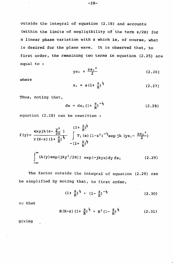
is desired for the plane wave. It is observed that, to

first order, the remaining two terms in equation (2.25) are

equal to :ZS12YSI + -2- (2.26)

whereSI = s(l+ ~)~

R (2.27)

Thus, noting that,z -~ds = dSl (1+ R:) (2.28)

equation (2.18) can be rewritten

f(y)=2

expjk(z- ~ )r(R-z) (1+ :)\

(1+ ~)~RI Tl (s) (1-s2)-~exp jk

-(1+ ~)~R

2( ~)YSl- 2

IOO(A(y)eXp(jky2/2R» exp(-jkys)dydsl (2.29)-00

The factor outside the integral of equation (2.29) can

be simplified by noting that, to first order,

(1+ ~) ~ ~ (1- ~)-~R R (2.30)

so that

R(R-z) (1+ ~) ~ ~ R2 (1- ~) ~R R (2.31)

giving

-29-

f(y)=

(1+ ~) ~RJ Tl (s) (1-s2)-~expjk {YSl-

- (l+ ~)~R

foo{A(y)eXp{jky2/2R»eXp{-jkYS)dYdSI

2expjk(z- ~)R2{1- .!)~

R

2~)2

(2.32)-00

The inner integral (over y) yields the function gee)

which may be expressed as a function of SI, say gl (SI), and

Tl (s)(1-s2)-~ can also be rewritten as a function of SI'

say Tl (SI), so that,

fey) =2

expjk (z- ~)R (1- ~)~

R

(1+ .!)~R

f (2.33)-(1+

We note

a) The desired linear phase variation of the plane wave

with z combined with a quadratic variation in y. This

tends to be cancelled out by the quadratic phase varia-

tion included in gl (SI), the exactness of the cancell-

ation depending on the approximations made during the

derivation of equation (2.33).

b) An amplitude variation of the form (1- ~)-~. This can

be interpreted as the amplitude fall-off due to a

cylindrical wave propagating outwards in the -z

direction and at this point we qualify the term "plane

wave" as used in the preceeding two-dimensional analysis.

-30-

The "plane wave" is defined in one dimension only and

from the nature of the geometry, one might expect that

there would be something other than plane wave

properties in the other dimension. What has happened

is that the process has compensated in one dimension

for sphericity of the outwardly propagating wave and

turned it into a cylindrical wave over a finite region

in space. It should be noted that, in the plots of

computed synthesised field distributions, compensation

has been incorporated for this variation.

c) Change of the value of z will cause an angular scale

change in g' (SI) and T' (SI) since the conversion factor

between SI and s is a function of z. This means that the

transform of g' (SI) into the y-domain (i.e. the basic

plane wave) will suffer compression or expansion

(depending on the sign of z) in y. The modified sinc

function of the impulse response will undergo a similar

scale change. In the former case, the change may be

difficult to observe since it is only of order (1+ ~)~

and the other effects which are particularly significant

at the edges of the plane wave may tend to mask it. In

the latter case, the transform of T' (SI) will widen for

negative z and conversely narrow for positive z indicating

that the influence of the scale change is likely to be

more serious for negative z. In fact, the computer

resuits presented later show that this effect is more

than compensated for by other effects which are more

serious for positive z. Such an effect is :

-31-

d)ZS12The term - --2-- in the exponent of the transform is a

straightforward defocus sing term appearing for Z ~ O.

This causes the form of the impulse response function

to deteriorate from that of a sinc and thus the

convolution with the plane wave produces more severe

ringing effects. It will also be noticed that the term

is proportional to S12 which means that its influence

will be much more marked for larger-angle weighting

functions. One other point to note is that, from

equation (2.27), the defocussing term is greater for

positive z than for negative (vanishing in fact for z

= -R, but this corresponds to the meaningless situation

SI = 0).

By the nature of the convolution, while the modified

sinc function of the impulse response is positioned near to

the centre of the plane wave, the integrated product will be

comparatively constant but when the sinc encounters the edges

of the plane wave, the variations become much greater so that

the ringing effects naturally appear most serious near the

edges. One more effect, not immediately apparent from the

above analysis, is caused by grating lobe effects due to the

sampled nature of the data. This will be illustrated later

in this chapter.

An approximate qualitative relationship has been

established between the angular range of the weighting function

and the maintenance of plane wave properties over a suitable

range of z. This cannot, however, be regarded as defining

the magnitude of the influence of various factors because;

· -32-

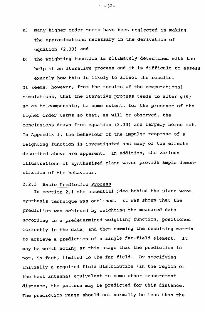
a) many higher order terms have been neglected in making

the approximations necessary in the derivation of

equation (2.33) and

b) the weighting function is ultimately determined with the

help of an iterative process and it is difficult to assess

exactly how this is likely to affect the results.

It seems, however, from the results of the computational

simulations, that the iterative process tends to alter gee)

so as to compensate, to some extent, for the presence of the

higher order terms so that, as will be observed, the

conclusions drawn from equation (2.33) are largely borne out.

In Appendix 1, the behaviour of the impulse response of a

weighting function is investigated and many of the effects

described above are apparent. In addition, the various

illustrations of synthesised plane waves provide ample demon-

stration of the behaviour.

2.2.3 Basic Prediction ProcessIn section 2.1 the essential idea behind the plane wave

synthesis technique was outlined. It was shown that the

prediction was achieved by weighting the measured data

according to a predetermined weighting function, positioned

correctly in the data, and then summing the resulting matrix

to achieve a prediction of a single far-field element. It

may be worth noting at this stage that the prediction is

not, in fact, limited to the far-field. By specifying

initially a required field distribution (in the region of

the test antenna) equivalent to some other measurement

distance, the pattern may be predicted for this distance.

The prediction range should not normally be less than the

-33-

measurement range because spatial frequency components may

appear here which are not propagated out to the measurement

sphere, thus the information is not available in the measured

data to predict the pattern with confidence(27).

From a simplified viewpoint, the prediction process may

be formulated as followsmol

nol g(m~8,n~¢)f(8F+m~8'¢F+n~¢)

n=-n o(2.34)

where P(8F'¢F) is the predicted element of the far-field

radiation pattern for angular coordinates (8F'¢F)' fC8,¢)

is the measured near-field response at coordinates C8,¢)

and where mo~8 = e and n ~¢ = ¢ , the limits on weightingm 0 mfunction g(8,¢). The process has, therefore, become merely

one of complex number multiplication and addition, simple

operations well within the capabilities of a relatively

unsophisticated hardware unit. It may also be noted, at

this point, that for principal axis predictions, only a

limited band of data along the axis is required and, for a

system with particularly severe storage limitations, a

routine might be written allowing data to be taken when

required and discarded at a later stage when nq longer needed.

This implies that a very limited system might still be

capable of making all-space predictions.

Various complicating factors will be discussed in later

chapters! particularly those caused by the three-dimensional

sampling geometry. The first experiment performed was

designed to be a relatively simple case avoiding the problems

and, as will be described, used an antenna assumed to be

-34-

one-dimensional and the prediction was performed around a

single cut of data. The modified version of equation (2.34)to do this was :

mor g(m~e)f(eF+m~e)m=-m o

(2.35)

The process in this case was to acquire a single circular

scan of data. A weighting function was created for the same

parameters and a simple routine of shifting, multiplication

and summing (as indicated in Figs. 2.2 and 2.3) performed

the prediction. The details of the experiment together with

the results are presented later in this chapter.

2.3 Sampling CriterionThe technique requires that the weighting function

distribution should be sufficient to yield an acceptable

quality plane wave field distribution over the desired volume.

The standard sampling criterion indicates (treating e and ¢

independently) that the greatest spatial frequency which can

occur due to an antenna of maximum dimension D is TIDIA

cycles per revolution requiring for complete characterisation

samples to be angularly separated by no more than AID radians.

This calculation is based on the requirement to sample

sufficiently frequently the radiated field. The conceptual

basis of the present approach is somewhat different so that

the idea behind the derivation of the sampling criterion

needs likewise to be modified. It is, nevertheless, to be

expected that the procedure adopted will indicate a similar

minimum sampling rate.

testantenna

weightingfunction

synthesisedplane wave

Fig. 2.2. The weighting function would, if practically realised,produce a plane wave in the region of the test antenna.Here, the configuration for a boresight predictionis shown.

sphere ofdata samples

direction ofprediction

weightingfunction

synthesisedplane wave

test antenna

Fig. 2.3. A prediction at any angle, eF, off boresight isproduced simply by positioning the weighting functioncorrectly in the measured data.

-35-

We began by noting the Fourier transform relationship

between a far-field (R -+ (0) weighting function and its

synthesised plane wave (analogous to the relationship

between an antenna aperture illumination and its far-field

radiation pattern). Since the weighting function is a sampled

rather than continuous function, the relationship is, in fact,

that of the discrete Fourier transform (DFT). One important

property of the DFT is its periodic nature. Thus the width

of one period of the plane wave function is such that

radiation from the edge of the period would contribute a

spatial frequency, in the far-field, of half the sample

frequency. Beyond this point, the synthesised plane wave is

repeated. If the width of the desired plane wave is small

enough to lie completely within a single period of the

periodic function, no problem arises. If, however, the

sampling rate, in the far-field, is less than twice the

maximum spatial frequency due to the required plane wave, it

begins to be overlapped by its counterpart from the neigh-

bouring period with consequent deterioration in quality. It

is, in fact, demonstrated in Appendix 2 that for the far-

field case, with an undersampled weighting function, the

iterative process succeeds in suppressing the outer points

to a very low amplitude reducing the weighting function

effectively to what is the usual far-field "weighting function",

a single point. Thus the problem of undersampling is

insignificant in the far-field measurement situation.

Clearly, since the weighting function is, in reality, to be

positioned in the near-field region, the Fourier' transform

relationship begins to break down. As illustrated in

-36-

Appendix 2, the off-axis periods of the "periodic" plane

wave function cease to be good replicas of the central

period, displaying instead a marked amplitude taper (due

to space attenuation) and, additionally the disappearance

of the linear phase portions apparent in the far-field case.

It is still evident, however, that the onset of overlap

occurs at the expected sample spacing so we see that in

this initial consideration, for the plane z = 0, the

sampling criterion is established as :

~e < A/D (2.36)

To take account of the depth of field requirement, it

is necessary to carry out some adjustment of this criterion.

The maintenance of the plane wave over a spheroidal volume

requires not only that adjacent periods of the plane wave

function should not overlap on the plane z = ° but also that

the same condition should apply for all values of z falling

within the compass of the sphere. Dealing again with one

scan coordinate alone, we say that adjacent periods of the

synthesised plane wave should not overlap so far as to

impinge upon the circular region of radius D/2 shown in

Fig.2.4. This implies, not, as one might superficially

assume, that the sampling criterion outlined above shouldbe fulfilled for all points within the circle but rather,

making allowance for the width of the region of overlap (see

Fig.2.5), it should apply for all points within the special

area also shown in Fig.2.4.

Consider (referring to Fig.2.6) a point S situated at

angle e in a circular data scan of radius R centred at

Fig. 2.4. The circular region enclosing the test antenna and thespecial area for fulfilment of the sampling criterion. Thespecial area is, in fact, that within and between twoellipses placed side-by-side, as shown.

- - - -1- - -.-11 -2j -- -

I

I

'>----~TDI II I

I I0I /2

,.I

- -'

Fig. 2.5. The unusual shape is to allow for the overlap of fixed-sizesynthesised plane waves; the maximum allowable overlap on theend plane z = D/2 is illustrated on the right showing thatthis implies a sampling criterion for a region of width D/2.

",,,,,,IIII,,

Zo

Fig. 2.6. The geometry for analysis of the near-field samplingcriterion for plane wave synthesis.

-37-

point o. Adjacent periods of the plane wave distribution

on the plane z = Zo overlap to within the circle enclosing

the test antenna if the near-field sampling rate is less

than twice the maximum spatial frequency, around the measure-

ment circle, of radiation from point Q relative to radiation

from point P (i.e. less than twice the maximum value of the

difference between the spatial frequencies of radiation from

the two points), Q being an extreme point on z = z withinothe special area.

Let us denote the "spatial wavelength" around the

measurement circle due to radiation from point P by the

symbol Al and, similarly, the "spatial wavelength" due to

radiation from point Q by the symbol A2. Then:

and

A2 = A/sina2 (2.38)

With the object of expressing sinal in terms of e, R,

D and z , the sine rule is invoked to giveo

sinal =z sineo (2.39)

and by the cosine ru~e,

rl = (R2+Zo2-2Rzocose)~ (2.40)

substituting from equation (2.40) for rl in equation (2.39)

yields,

sinalz sineo (2.41)

We also require sina2. By the cosine rule again,

-38-

(2.42)

where

b = a/sina (2.43)and

a = tan-l (a/z )o (2.44)

a being given by,

(2.45)

Invoking the sine rule,

sina2 = bsin(8+a)r2 (2.46)

substituting for r2 from equation (2.42)

bsin (8+a)=(R2+b2-2Rbcos{8+S»~

(2.47)

where band S are as defined by equations (2.43), (2.44)

and (2.45) •

Having now defined sinal and sina2, we can determine

the difference in spatial frequency between radiation from

P and Q as :1

1.121 1 (2.48)

where 1.12 is the "spatial wavelength", along the measurement

circle, of the radiated field from Q relative to that from P.

Thus,

(2.49)

Given the values of R, e, D and zo' we can thereforedetermine the relative spatial frequency of radiation from

points P and Q. To establish a sampling criterion, it isnecessary to find the minimum value of A12 with varying Zo

-39-

and 8 over the appropriate ranges. The expressions are,

unfortunately, not of a form which yields readily an

analytical expression for the minimum "spatial wavelength"

but it is, on the other hand, quite a simple matter to obtain,computationally, the value of A 12 min for given values of A,Rand D (if only by calculating values for a range of z and

o8 and examining them by hand - it is, of course, faster and

more accurate to employ a suitable search technique as was

used to obtain the results shown here). The maximum allow-able angular sampling interval is then given by :

(2.50)

Fig.2.7 is an example of such a calculation illustrating

the variation of critical sampling interval with R for a

range of values of D. It is found that for distant measure-

ments (R -+- (0) the maximum sampling interval is, as expected

118 = AIDmax (2.51 )

but, as R is reduced, the values of A12 corresponding to

negative values of z begin to increase while a minimum valueo

of A12 forms for small positive zoo As R is further decreased,

this minimum deepens and the corresponding value of Zo

increases until the limit of z = D/2 for minimum A12 iso

reached in the case of very short range measurement. It is

seen, therefore, that a near-field measurement system requires

a sampling rate in excess of that indicated by equation (2.36).

It turns out, in fact, that the critical sampling interval,

expressed in terms of a proportion of the standard AID

criterion is dependent purely upon the ratio RID and so the

0·<o. . ."" "" "" . . -0 0 0 "" ""

p:;0 0

0 0 0 . . -N C"l Vi ,..... N (()

II II II II II;:::loM

q q q q q'{j

0 ~·Vi+'~IDe,--.., ID. H

e ffi'---"ctlp:; IDe

0 .c· +'..:j- .r!~

,--..,·t'l::r:t:J0·0...-I

0 1;3·f'1 '---"

r-i .ctl (()

~ ~ID+'+' ID.~@

.r!ID'{jr-i

0 p.,ID· @ ~N(() ~e Q)

§ @.r! r-l~ p.,ect-l

0ct-l0 ID

0 eo· ~ @,..... 0.r! H+'ctl ctl.r!H Hctl 0!>ct-l

·e-·0 N·0 ·0'\ CO t'- <o Vi ..:j- C"l N ,..... 0 eo.r!rx..

(S8e.I~8p) 1BA.I8,+U1~u11dmBS mnm1XBW

-40-

sampling requirements for all frequencies, sizes of planewave and measurement distances can be 'summarised in a

single graph, Fig.2.8.

2.4 Visualisation of Field Distributions

As an aid to the understanding of the processes taking

place in the formation of a plane wave fro~ a weighting

function, a computer program was developed to calculate the

synthesised field distribution over a plane cut through the

region containing the weighting function and forward through

the plane wave. The distribution is then displayed on grey

scale (or false colour) as a picture on the T.V. display

system attached to the Departmental V-72 image-processing

computer (see Appendix 4).

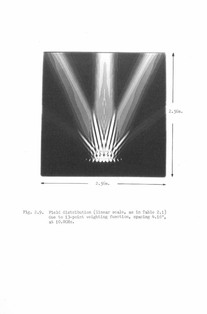
Three examples are presented in this thesis of the out-

put from this program. The first (Fig.2.9) displays the

synthesised field distribution due to a l3-point (one-

dimensional) weighting function, spacing 4.160, operated at

10GHz and with a measurement range of 1.Om. The displayed

range is ±1.28m in each dimension. Table 2.1 lists the

correspondence between field strength and display level.

~he region of the weighting function is visible near the

bottom of the picture and the plane wave region, specified as

30cm wide, in the centre. Towards the top of the screen, it

is apparent that the plane wave distribution has broken down

and regions of bifurcation etc., are apparent as the fields

begin to focus into a main beam. Additionally, because ofthe relatively coarse sampling, two grating lobes can be

seen forming on either side of the main beam. In the region

oo .

oo.o

o·'-0

o·

»~~0If-ien~.r!

~~

~I=lQ)Elp::;~filcOQ)El..c:~.r!~rlcO

~Q)~I=l.r!Q)rl

~enEl~.».r! C)

~ I=lQ)

El ~cri

If-i Q)0 ~I=llf-io »:j ~cO.r! ~~ cOcO> Q)

t:lIf-i .r!o Cl)

~~S]65 ~.

coN.eo.r!r:z:.

o·-::T

o·C""\

o·N

o·.-l

o·o

2.56m.

Fig, 2.9. Field distribution (linear scale, as in Table 2.1)due to 13-point weighting function, spacing 4.16°,at 10.0GHz.

2.56m.

Table 2.1Correspondence between display levels

and field strength for Figures 2.9 and 2.10

Field strengthDisplay level (normalised linear, 1.0 =

desired plane wave amplitude)

0 (black) below 0.11 0.22 0.33 0.44 0.55 0.66 0.77 0.88 0.99 1.0

10 1.111 1.212 1.313 1.414 1.515 (peak white) above 1.5

-41-

between the weighting function and synthesised plane wave,

some large ripples can be observed vanlshing just at the

near edges of the plane wave. This allows one to place

another interpretation on the breakdown of the plane wave

into high edge values for positive z : interference fringes

due to the interaction of two (or more) plane waves, the

required plane wave and the grating lobe(s).

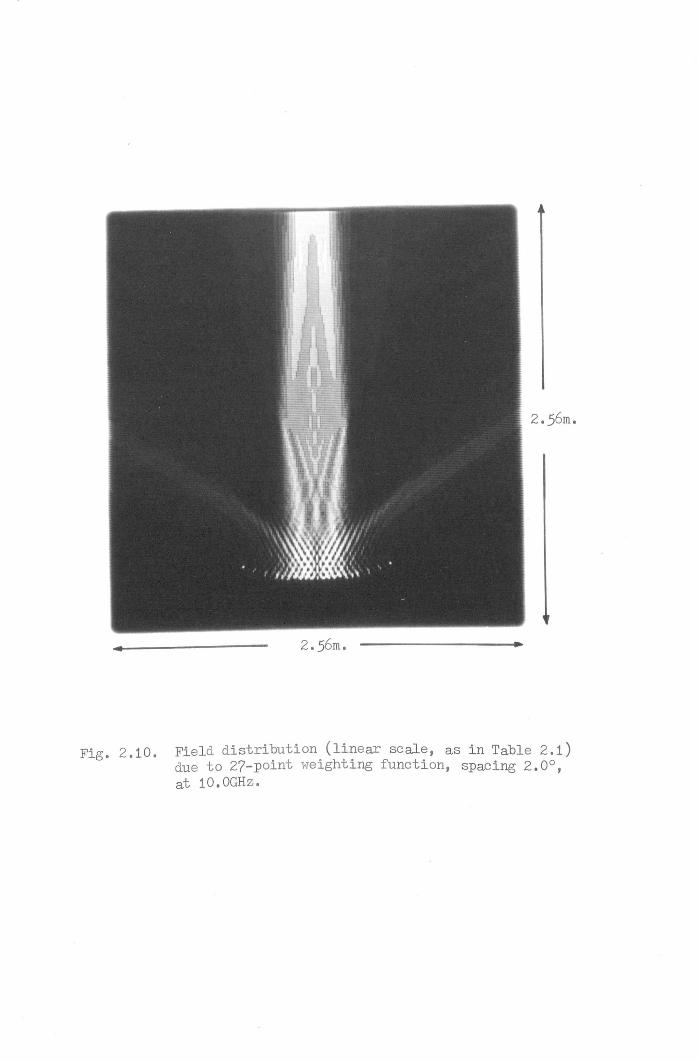
The second example is for similar parameters to the

above except that a 27-point weighting function was used

with a 2.00 sampling interval. Similar effects to those

described above are observed here (Fig.2.10). Because of

the reduced sampling interval, now only one grating lobe is

created on either side of the main beam. The details of the

significance of the different grey levels are again as in

Table 2.1.

The last example of the use of this tool for visualisation

of field distributions is for exactly the same parameters as

example 2 except that the displayed range is reduced to

±25.6cm to show more detail of the synthesised plane wave

itself (Fig.2.11). The details of the highly non-linear grey

scale representation are contained in Table 2.2. It is felt

that this method of displaying synthesised field distributions

proves a useful aid to the understanding of the processes

involved.

2.5 Two-Dimensional Experimental Results

A 30cm slotted waveguide operated at 10.143GHz was used

as the test antenna fora basic verification of the process.

The Rayleigh range (2D2/A) for this configuration is

rSHUflELO·i I:iOIVERSITY!

2.56m.

2.56m.

Fig. 2.10. Field distribution (linear scale, as in Table 2.1)due to 27-point weighting function, spacing 2.0°,at 10.0GHz.

51.2cm.

Fig. 2.11. Field distribution (expanded linear scale, as inTable 2.2) due to 27-point weighting function,spacing 2.0°, at 10.0GHz.

51.2cm.

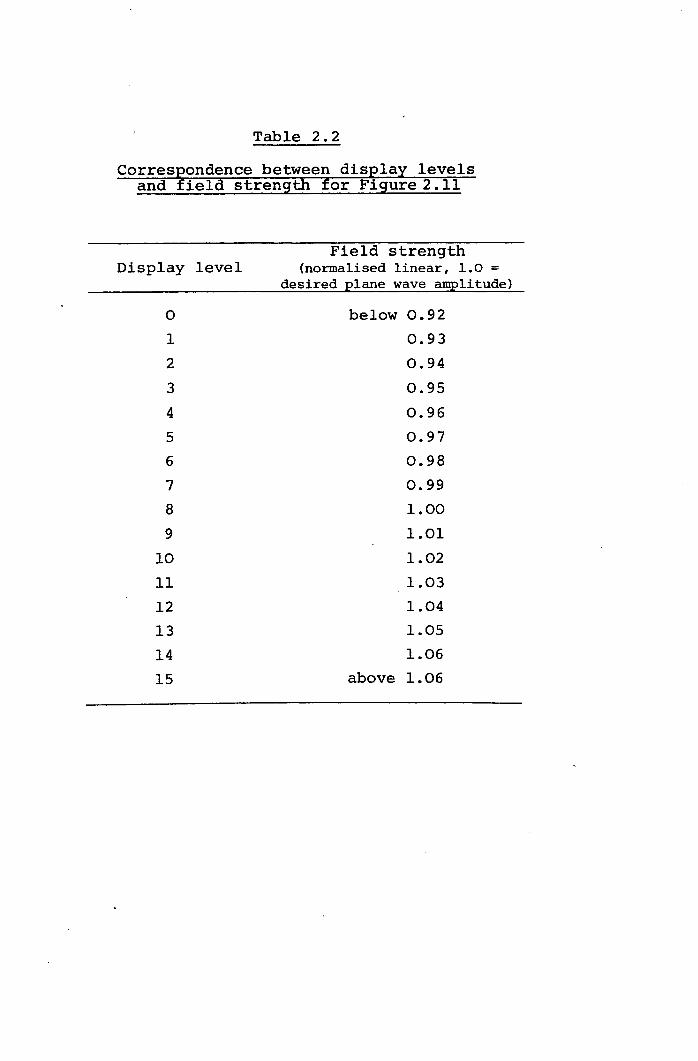
Table 2.2corres¥ondence between display levels

and ield strength for Figure 2.11

Field strengthDisplay level (normalised linear, 1.0 =

desired plane wave amplitude)

0 below 0.921 0.932 0.943 0.954 0.965 0.976 0.987 0.998 1.009 1.01

10 1.0211 1.0312 1.0413 1.0514 1.0615 above 1.06

-42-

approximately 6m, and this corresponded conveniently to the

length of the anechoic chamber (at that time) at the

University of Sheffield antenna test range at Harpur Hill

near Buxton in Derbyshire (described in detail in chapter

6). For simplicity of data processing, the antenna was

assumed to be perfectly one-dimensional and it was assumed

that only a single circular data scan would be necessary

with processing by a one-dimensional weighting function.

An inaccuracy inherent in this assumption will be mentioned

shortly.

An open-ended waveguide was employed as the near-field

probe for the acquisition of the data, the receiver used

being a Scientific Atlanta (S.A.) model 1754 two-channel

phase and amplitude instrument. The second input channel

of the receiver was used for the reference signal for both

phase and amplitude. The reference antenna was also formed

from open-ended waveguide embedded in absorber below the test

antenna. The outputs from the receiver passed via an S.A.

1822 phase meter and an S.A. 1833 amplitude ratiometer to

the data logging system comprising an Argus 600 minicomputer

(also responsible for control functions) and an 8-track paper-

tape punch. This is illustrated diagrammatically in Fig.2.12.

Data were acquired around a full 3600 azimuth scan at

0.50 intervals and at a variety of different measurement

distances, the shortest range being 1.01Sm and this set of

data is treated in detail here.

Initially a weighting function needed to be obtained and

for this purpose, the plane wave was specified to exist over

.L;.u'- C

<II :J~ 0.0.

<II0.a

>.u '-~.e:J ceT:J<II 0'-u-

NCIOl!)'-MVl...r>.~..YO

'-oc{ <IIN .....

~<IIN E

<II

to

~

.D0

<II

'-

« VI

0.

aQ)

'-'- .L;.

'"Cl

(II0 If)

0..r!

::::J

610. VIE c

Q)0 <II 0

~u :J5 .....C 'iIi u

~'E c c:::I

'"Cl

o _

Q)

0. .0 VI

~0 <II 0

~UJ '-VI '-

rl:J 0 C .....

UlOl

VI 0'- u ..... .« aa

Iii>'-0

If)

0C""'I

Cf-I0

~0.r!

~

~>Q)

f..l0Cf-IPI;::lI~Q)Ul

III «\~

(II '- Q)VI <II .~a >

f..l.L;. 'OJ .-..to. Q)

,u

~U1

(II

"e-,

'-r:iI

II

Qj <IIC -0

.,C :J

N

a

a .....

c'I

..i..L;.~ .-I

C

v; ~ E C\l

<II

" s:

.......... ....

N a .c

C:::I

a

" ~~ E -c eo..-I

....." 'N

r:.

VI

a

<II I

-43-

a range of ±20cm (i.e. D = 40cm) and the weighting function. 0consisted of 81 points spanning an angular range of ±20 •

This weighting function is shown in Fig.2.13. Fig.2.14

illustrates the quality of the plane wave for various values

of z in the region of the test antenna. It is seen that the

plane wave properties are maintained well over a sufficient

depth. The worst of the ringing effects are observed to

occur near the edges of the plane wave and it should be noted

that, particularly for z t 0, the test antenna occupies only

a central portion of the plane wave so that these peripheral

regions assume little importance.

The measured near-field amplitude pattern is shown over

the full 3600 range in Fig.2.1S and displays classical near-

field defocussing effects. The predicted far-field pattern

and that measured at 6m range are compared in Fig.2.16 and

exhibit an encouraging similarity. Several factors may be

cited as possible sources of error

(a) The inaccuracy of the one-dimensional assumption for the

antenna. While probably quite accurate for the slotted

waveguide itself, the assumption breaks down for the

support structure which should, strictly, be taken as

part of the antenna. As much of the support structure

as possible was shielded with absorber in an attempt

to minimise the ill effects of this factor.

(b) The lack of probe compensation. The open-ended wave-

guide probe had a finite size and therefore non-

uniform radiation characteristics but no compensation

was incorporated for this. A scan of the probe pattern

·~

,,-....II.lID

~QO 0ID'd'--""

IDII.lro..c:Pi

-180-20

-20 ~ -L ~

-20 o 20e (degrees)

180

o 20e (degrees)

Fig. 2.13. One-dimensional weighting function used inevaluation of 3Ocm. slotted waveguide array.

(a)-20 0 20

x (cm.)

(b)

-20 0 20x (cm.)

(c)-20 0 20

x (cm.)

-20 0 20x (cm.)

180

.--....I/}

IDID

tbID

~OIDI/}

III

-&

-20 0 20x (cm.)

180.--....I/}

ID

~eoID

~OIDI/}

III

-&

-20 0 20x (cm.)

Fig. 2.14. Synthesised plane wave due to weighting function shownin Fig. 2.13; (a) z = 0, (b) Z = -15cm., (c) Z = +15cm.

r-----------------~------------------~g..-I

~

~0 m0'\ 'd

·rl

?om~~~

{I) 'dm mm -f..l~ -f..lQO 0.m r-i'd {I)<;» ·<D El

C)0<'l

tf-i0.

0

Sm-f..l

~Pi

m'd.s·rl ·r-I ElPi\.CI@cj·'d~r-Im m

~~0 ~p:;0'\I m ·~ N

~g~ .!iJ~rom+l::;E; ro

·\.Cl~·C\I·QOi£

0OJ..-I

0 0 0 0 0 I~ C\I <'l ~I I I I

(HP) apn+1Tdure pas1reUIJ:O~

r-----------~--------------~g..-I

(/)s(])-j.:!

"'itlPi

{ (])0 'dQ'\ ;:j

-j.:!o,.-j~,.--.. Pi

(/) @(])

~ 'dQO r-i(]) (])

'd o,.-j'-" tt-i<D ~

tt-i~ ,.--..

'd(]) -..c: til

-..."...... (/)::t:ro0'dO0 '-" 0

0-..-I

t=i~"'itl"'itl ~~~;:j(/) (])ro'd(]) o,.-jt=iGb

'd (])~ ~

~,.--..'d'do,.-j (])~-j.:!

0 O-j.:!Q'\ (/)0, '-"~

(/)'d(]) --j.:! t=iC) C)o,.-jO

'dC""\(])

~1:l-<o

..-I

C\l

-QOo,.-jrx.

0CO..-I

0 0 0 0 0,..-I C\l C""\ .:::t, , I ,

Cm» apni-ITdure paSrrellUoN

-44-

indicated that the amplitude taper over the test antenna

region was a small fraction of a dB and therefore the

error caused by neglecting probe compensation is

probably slight.

(c) Possible discrepancies between tne true far-field

pattern and that occurring at a range of 6m. It is

well known that certain antennas (those relying on

supergain principles being particularly severe cases(28»

require a distance well in excess of the conventional

2D2/A, to establish their true far-field patterns. In

an attempt to determine whether this factor is

significant in this particular case, a new weighting-

function was created to synthesise a slightly spherical

wave (corresponding to that due to a source at 6m range)

and a prediction was performed using this (i.e. a pre-

diction for 6m range). This is shown in Fig.2~7 and

it is immediately obvious that the alterations to the

predicted pattern are very slight indicating that this

possible source of error is probably not important in

this instance.

(d) Chamber reflections. It is expected that reflections

are, in the main, at a level of -40dB or better but

certain regions of the pattern separated by 1800 exhibit

the more noticeable errors which might indicate the

effects of reflections of the main beam and back lobe

from certain areas of the chamber. Such reflections

may, in fact be more significant in the far-field

measurements than in the near-field data since the

longer measurement range implies more grazing incidence

~0 ~o-,

a>'1:1.r-!.........Gbm

a> a>

~ ~~a>'1:1 '1:1'-'" a>

+lCD +l

0,..;m

·~00C""'\

0ct-t0

~~a>+l~ ·Pi~0

a> ·'1:1'-0Ect-t.r-! 0,..;Pia>

~~'1:1 ~a1 III

0 .r-!o- ct-t ~I I 0

~ct-tct-t 0

N'1:1::r:!roC)+l00 ··r-!O'1:1.--ta>~~

·C'-.--t·C\l·0 eoco .,;

.--t rz.I

0 0 0 0 0.--t C\l C""'\, ..:::tI I I I

(8:P) apnTIdure pas -n-eUI.:ro N

-45-

of radiation upon the chamber walls which in turn means

that ·the reflection levels will tend to be higher.

(e) Variation of plane wave amplitude with z. Although it

is not obvious from Fig.2.l4, each amplitude graph in

this particular case being independently normalised,

the synthesised plane wave suffered from a slight

amplitude fall-off with increasing distance from the

weighting function (i.e. decreasing z). This is the

practical manifestation of the effect derived from the

equations of section 2.2 where, using a one-dimensional

weighting function, it was shown that the amplitude was

proportional to (l-Z/R)-~, a cylindrical wave effect.

This will be of greatest significance in the wider

angle predictions (8 ~ ±90o) whereas for predictions

near to the main beam or to the back lobe, the effect

will not be pronounced.

2.5.1 Conclusions From the Two-Dimensional Results

Within the limits of the two-dimensional approximation

and the various errors listed (chapter 5 also covers some

errors which may be of importance), it has been demonstrated

that plane wave synthesis can provide a useful means of

effecting a near-field/far-field transformation. Since

these early results, the process has been refined rather

more as regards the attainable quality of synthesised plane

waves and also the move to the rather more complicated three-

dimensional sampling. In the next chapter, therefore, we

turn our attention to this latter aspect of the prob~em.

-46-

3. THREE-DIMENSIONAL PREDICTION WITH PROBE COMPENSATIONUSING AN ELEVATION-OVER-AZIMUTH SCANNING GEOMETRY

In Chapter 1, the sampling geometry produced by an

elevation-over-azimuth scanning system was introduced; it

is now necessary to formulate this geometry in detail with

a view to implementing an iterative procedure, related to

that encountered two-dimensionally in Chapter 2, to produce

a weighting function applicable over a spherical measurement

surface. The details of the iterative procedure will be

covered in section 3.3.

3.1 The Approach Used

It is assumed that the radius at which the measure-

ments are taken is in the far-field of the probe so that the

radiated field can be taken to vary, in the radial direction,

only as exp(-jkr)/r. It is further assumed that the radiation

pattern of the probe has been fully characterised (at least

over the extent of the relevant solid angle about boresight)

in amplitude and phase as a function of its own angular

coordinates (8p' ¢p). It is convenient to assume that the

probe radiation pattern has itself been measured using an

elevation-over-azimuth system, although naturally, with

suitable modification to the expressions, any other probe

measurement geometry could equally well be accommodated.

The synthesised plane wave is built up by super-

position of the components of the probe placed, in turn,

at all the positions defined for the weighting function.

This means that it is necessary to determine, for any

particular angular position (8w' ¢w) of the probe, the

field components occurring at any point Q (x, y, z) in the

-47-

plane wave region. We need, therefore, to determine what

values of ~p, ~p in the probe pattern correspond to the

position of point 0 relative to the probe when it is at

position (Sw, ~w). Initially we specify that the plane

wave exists over a region of the plane z = 0 (see Fig.3.1) •

An offset (zo) of the plane will be considered at a later

stage.

In the elevation-over-azimuth geometry, the probe

lies in the plane S = Sw looking directly at the origin at

all times and with what we may for convenience term its

principal polarisation direction perpendicular to the plane.

The relationship between Sp and ~p and Sw, ~w' x and y is

not straightforward since, not only is the probe generally

off-axis, but it is also twisted through two angles.

The approach used here for unravelling the com-

plexities of the geometry is to consider a second plane,

also passing through the origin, 0, but rotated through

two angles such that a new coordinate system (x", y", z")

is formed in which the new plane is the plane z" = 0 and

the probe lies on the z"-axis with its principal polarisa-

tion direction parallel to the y"-axis. The probe will·

still, of course, point directly towards the origin, along

the z"-axis. The new configuration is illustrated in

Fig.3.2. The point 0" (x", y", 0) is taken to be the

projection onto the plane z" = 0, looking from the probe

positionJ of the point 0 (x, y, 0) in the original unrotated

coordinate system. Being the projection looking from the

probe, the point 0" in the new coordinate system must

possess exactly the same angular orientation (Sp, ~p)

y

x

~ plane wave definedon this plane

z

Fig. 3.1. Probe/plane-wave-point relationship for anelevation-over-azimuth scan system.

y"Q" (x", y" , 0 )

z"

Fig. 3.2. The new x",y",z" coordinate system producedby a double rotation about the origin.

-48-

to the probe as the original point Q. The angles 8p and

<Ppcan be l;"elatedcomparatively easily to x" and y" since

in the x" y" - Zllcoordinate system the probe lies on

the zll-axis and is upright. The problem of relating 8pand <Ppto x, y, 8w and <Pwis effectively translated to

that of relating x" and y" to x, y, 8w and <Pw.

3.1.1 Rotation 1

The process of obtaining x" and y" in terms of x, y,

8w and <Pwis carried out in two stages. The first stage

consists of a rotation of the plane z = 0 through an angle

8w about the x-axis to form the plane z' = 0 in the newly

created x' - y' - z' coordinate system. The probe now

stands upright on the plane y' = 0 as illustrated in

Fig.3.3. We must now find expressions for the coordinates

x' and y' of the projection, Q', of the original point Q,

onto the plane z, = o.From Fig. 3.4 which is a view obtained looking along

the x (or x') axis, we see that,

y' = Y (cos8w + sin8w tan (a + 8w» (3.1)

where

a = (3.2)

yp and zp being two of the Cartesian coordinates equivalent

to the probe position (R, 8w, <Pw), given by,

yp = R cos<Pw sin8w (3.3)

and

zp = R cos<Pw cos8w (3.4)

y' (y)..II

x' (x)

...

probe

-- -- - ...

Fig. 3.3. Rotation 1 to form x',y',z' coordinate system.

y' y

Fig. 3.4. View along x (or x') axis for first rotation.

z'

(z)

z'

z

-49-

The other Cartesian coordinate, xp is given by,

xp = R sinct>w (3.5)

and this is required in the formulation of an expressionfor Xl. Referring to Fig. 3.5, from equivalent triangles,

Xl - X___ ~pL. =X - xp

dl + dd (3.6)

which, when the appropriate substitutions are made toeliminate d and dl, yields,

(3.7)

3.1.2 Rotation 2

The second rotation takes place about the yl-axis

(which then becomes the y"-axis) through an angle ct>w,to

form the plane z" = 0 in the x" - y" - z" coordinate

system.

Fig. 3.6 illustrates the geometry of this rotation

in some detail. It can now be shown that,

Xl sin<p cosSwY" = s ' (1 + )A cos(S + <Pw) (3.8)

where, as shown in Fig. 3.6,

2 2)l:zA = (yp + zp (3.9)

andx ' - x

S = tan- 1 ( p)A (3.10)

The change in the x-coordinate is described by,

x" = Xl (cos<Pw+ sin<Pwtan (S + <pw» (3.11)

z'

Fig. 3.5. To determine x' in x',y',z' coordinate system.

y" (y')

z"- - ........

........-&. z'

Fig. 3.6. Rotation 2 to form x",y",z" coordinate system.

-50-

3.1.3 Resulting Field Components

If :we now move over to the probe coordinate system,

as shown in Fig. 3.7, we can determine the angles 8p and

<Ppto be as follows:

<Pp= sin-1 (x")r1

and

8p = tan-1 ~(R )

where

r1 = (x..2 + s"" + R2)~

(3.12)

(3.13)

(3.14)

It is important to note, at this point, that the

angle <Ppas defined above is not the angle actually used in

the probe measurement system, as defined in Chapter 1, but

is in fact its negative. The field component in the <Pp-

direction is likewise reversed.

We now recall that, to describe fully the near-field

pattern of the test antenna, it is necessary to obtain data

samples with two orthogonal probe polarisations. This fact

becomes of more significance in later sections but, at this

stage, let it suffice to say that the analysis below applies

.to only a single polarisation of the probe which we may take,

for convenience, to be the principal polarisation direction.

It is shown in Chapter 5 that it is possible to obtain use-

ful results utilising only a single polarisation of a suitable

probe. If the appropriate components of the probe field are

extracted, the following analysis is, of course, equally

applicable to the secondary polarisation of the probe.

It is assumed that the radiation pattern of the probe

y"

x"

Fig. 3.7. The probe coordinate system.

-51- .

has been characterised, for convenience, on an elevation

over azimuth system, thus, with suitable interpolation

if necessary, the components Eep and E¢p will be known.

It can be shown, by returning through the double

rotation, that the resultant field components at the

point Q in the original coordinate system are given by,

E = Ee sin¢ sinex p w p

+ E~ (cos¢ cos¢ + sin¢ sin¢ cose )'i'P w P w P P (3.15)

and

E = Ee (cose cose + cos¢ sine sine )y p w p w w p,

+ E~ (cos¢ sine sin¢ cose -sin¢ sine cos¢'i'P w w P P w w P- cos e sLn e sine )w p p (3.16)

For the present, we omit the Ez component since this

is not required directly for the implementation of the

iteration procedure. The existence of a component in the Ezdirection implies some effective propagation across the

plane wave region (i.e. not in the wanted z-direction) and

must therefore be associated with a perturbation of the

desired plane wave component Ey and thus optimisation of

the components in the plane of iteration (Ex and Ey) will

automatically imply the minimisation of Ez• The coefficients

characterising Ez will be given for the case of an offset

plane of iteration, which is the more general case, and

these can be used to derive the coefficients for the present

non-offset case.

It should be noted that, for brevity, the factorR exp-jk(r-R) has been omitted from equations (3.15) and

r

-52-

(3.16). Here, the quantity r describes the distance from

the probe at (R, e , ¢ ) to the point Q (x, y, 0) and isw w

given by,

r = «x - x )2 + (y _ Y )2 + Z 2)~P P P (3.17)

3.2 Introduction of z-Offset

It has been found that the synthesised plane wave

tends to maintain its properties for a greater distance

from the plane of iteration in a direction moving away

from the weighting function region than in the direction

moving towards the weighting function. In view of this,

it has been found advantageous to define the plane of

iteration as offset from the origin some small distance

towards the weighting function region. In addition, if it

is required to examine the quality of the synthesised plane

wave on planes other than that passing through the origin,

it is likewise necessary to introduce an offset, zo' into

the coefficients previously derived.

The two coordinate rotations which were earlier

arranged to take place about the origin are now arranged

to take place about the point at which the line joining

the probe to the origin intersects the plane z = zOo

Equation (3.1) may be modified to include the offset, zO'

as follows,

y' = (y-Z tane ) (cose +sin8 tan(a+8 »o w w w w (3.18)

wherey - yP

N = tan-1 ( _)u. Z - ZP 0

(3.19)

the relevant diagram here being Fig. 3.8, a view looking

along the x (or x') axis.

y

a. + ew

Zl

Yp

z

Zp --------- ....

Fig. 3.8. z-offset, rotation 1, view along x (or Xl) axis.

Xl

Fig. 3.9. z-offset, rotation 2, view along yl (or ~ axis.

-53-

Equation (3.7) is likewise modified to read as

follows,

Xl = Rcos¢ -z Icose }2+yl2 ~(x-x ) ( wow )

p z 2+(y_y }2p P

(3.20)

Moving on to the second rotation, equation (3.8)

for y" (repeated here for convenience) remains valid,

Xl sin¢ cosS- I (1 + w)y - Y A cos(S + ¢ }

w(3.2l)

where S is defined, as in equation (3.l0),

S = tan-1 (3.22)

but the value of A is slightly modified from that given in

equation (3.9),

A = (y 2 + Z 2)~ - z Icosep pow (3.23)

For the x"-coordinate, equation (3.ll) is altered to read,

x" = (x I -z t.ane Icos e ) (cos e +si.ne tan (S+¢ )}o w w w w w (3.24)

as may be deduced from Fig. 3.9.

3.2.1 Resulting Field Components

As in section 3.1.3, we now move over to the coordinate

system used to describe the probe. The equation used for ¢p

still remains valid,

'" . -1 (x")'t' = S1n -p r1(3.25)

but r1 is now altered to,

r1

= (X,,2 + y,,2 + (R _ zo )2}~cose cos¢w w

(3.26)

-54-

The equation for S becomes,p

(3.27)

Having found the appropriate angles in the probe

measurement system (and noting again the lateral inversion

meaning that the value of ¢ shown is the negative of thep

actual value in the probe measurement system and the

direction of E¢p is reversed), the values of the two field

components ESp and E¢p may be obtained from the measurements.

Again the factor R exp-jk(r -R) has been assumed in ther

above and should be included at this point bearing in mind

that the value of r is now given by,

r = ((x-x ) 2 + (x-y )2 + (z -z ) 2) ~P P P 0

(3.28)

For completeness, at this point, we go on to note

the Ez component, although not important as regards the

iteration procedure,

EZ

= ESp (cos¢ cosS sinS - sinS cosS )w w p w p

+ E~ (cos¢ cosS sin¢ cosS'PP w w P P

+ sinS sin¢ sinS - sin¢ cosS cos¢ )w p p w w p (3.29)

(R exp - jk(r - R) assumed).r

3.3 The Iteration Procedure

The preceding sections have derived, in detail, the

equations relating the field distribution in the plane wave

region to the angular position of the probe. This enables

us to evaluate the synthesised field produced if the probe

-55-

is scanned over the spherical surface and the appropriate

data samples are weighted with any desired function. We

now recall that we require the synthesised field to take

on the form of a linearly polarised plane wave with

components,

E = 0xE = 0z

E = constanty

(3.30)

(3.31)

(3.32)

which, in turn, means that we require a weighting function

which, when applied to the samples at a particular set of

points defined on the spherical scan surface, gives rise

as nearly as possible, to this situation. Applying the

idea of reciprocity leads us to say that if we specify

the desired plane wave suitably over the particular plane

of interest and then integrate numerically out to the

spherical surface, using coefficients identical to those

obtained earlier (but with inverted exponential

R exp + jk (r-R) ). an approximation to the correct weightingr I

function may be achieved. If the angular range of this

weighting function is unlimited then, as stated in section

2.2, when the set of coefficients (now with the negative

exponential) are used to construct the synthesised field

distribution on the same plane, a very close approximation

to the desired plane wave is produced. If, however, some

different z offset is introduced to examine the synthesised

plane wave on a different plane, it is found that the

distribution breaks down. To improve the "depth of field" of

the synthesised plane wave, the angular extent of the

-56-

weighting function, g(8W'¢w)' is limited. This also has

the useful ,property of reducing the quantity of near-field

data involved in anyone prediction. It is now found that

the synthesised plane wave exhibits somewhat reduced

quality on the original plane but maintains itself much

better with varying z. This property is illustrated in

Appendix 3.

The quality of predictions obtainable with the

"first guess" weighting function would be severely limited

by the poor plane wave but this can be much improved by

applying an iterative procedure. The mechanics of this

are as follows. The synthesised plane wave is calculated

from the "first guess" weighting function. There will be

certain errors present in this field distribution and these

may be extracted and propagated out again to the spherical

surface in the same way as was done with the original

desired plane wave distribution. This creates what may

be termed an "error weighting function" which is sub-

tracted from the "first guess" to provide a "second guess"

weighting function. This, in turn, can be used to

synthesise a new plane wave whose errors will be smaller

than in the plane wave due to the "first guess". The

process can then begin again to produce a "third guess"

and so on until the process has converged to give an

optimum weighting function.

3.4 Typical Parameters for the Weighting Function

It has been found that, typically, a weighting

function will need to extend to between ±200 and ±300

in 8 and ¢ , and will converge to produce a plane wavew w

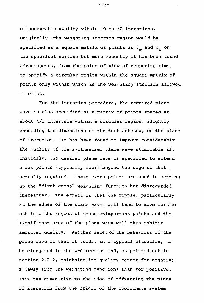
-57-

of acceptable quality within 10 to 30 iterations.

Originally,' the weighting function region would be

specified as a square matrix of points in e and ¢ onw wthe spherical surface but more recently it has been found

advantageous, from the point of view of computing time,

to specify a circular region within the square matrix of

points only within which is the weighting function allowed

to exist.

For the iteration procedure, the required plane

wave is also specified as a matrix of points spaced at

about Aj2 intervals within a circular region, slightly

exceeding the dimensions of the test antenna, on the plane

of iteration. It has been found to improve considerably

the quality of the synthesised plane wave attainable if,

initially, the desired plane wave is specified to extend

a few points (typically four) beyond the edge of that

actually required. These extra points are used in setting

up the "first guess" weighting function but disregarded

thereafter. The effect is that the ripple, particularly

at the edges of the plane wave, will tend to move further

out into the region of these unimportant points and the

significant area of the plane wave will thus exhibit

improved quality. Another facet of the behaviour of the

plane wave is that it tends, in a typical situation, to

be elongated in the z-direction and, as pointed out in

section 2.2.2, maintains its quality better for negative

z (away from the weighting function) than for positive.

This has given rise to the idea of offsetting the plane

of iteration from the origin of the coordinate system

-58':'"

and this has been implemented in the more recent software,

hence the importance of formulating the relationship

between plane wave components and probe position for

z-offset in section 3.1. Section 2.4 includes particularly

useful illustrations of field distributions in the plane

wave region.

3.5 Three Dimensional Scanning

In the above, we have described the creation of a

weighting function extending around part of the equatorial

region of a set,of points corresponding to an elevation-

over-azimuth measurement geometry (or azimuth-over-

elevation if everything is rotated through 900). Fig.3.10

illustrated the situation of such a weighting function

positioned on a sphere of data measured on an elevation-

over-azimuth system. It is immediately obvious that, to

predict the ESF far-field component at any other angle,

SF' along the principal axis, ¢F = 0, the weighting function

will be incremented through the data in the elevation (S)

direction and the direct positional and polarisation

correspondence between data and weighting function will be

maintained. If it is required, however, to produce a

prediction for ¢F t- 0, the situation shown in Fig.3 .11 arises

where there is no longer any correspondence between

measured data and weighting function. A similar sort of

problem is encountered when the prediction of the E¢F

component is required,when the weighting function has to

be rotated through 900 about its centre and again the

correspondence between data and weighting function is

lost.

Fig. 3.10.

Fig. 3.11.

sphere ofdata

..... -; ,,.,-"'-'-~" '

, I ' ~ ,,l I.",. _ J _~....~ ,,',I,r", '

A , I / ........ "'1'--" ",

"1.... I I -", "" 1 " , " , ,,""\,I "

I ') '";-4- , ....t; / , ,.," ~ ,, \,) \ I, I ',,, ,

I I I ,. \ ,_, , ", , , , ' , I ' , " \.. ' ",, ", '" ,. ", "\I ,'7' ,,,\,,,/~"''''''I ' ' __ l--+-l-oH~ .. - I.. ',.' \~""''''' ... ' - r - _1- - -I" - - ::~- - ,- - "1 __ , - ", -:~ -:. - __ _,1_1_-, -<,,'1~~".J. --.1 __

, ,,' V" - - ," ~ "'<, " \' ... ,--, ...," < I, 4' r' ; " " ' ,._\\/0( ", ,""

I 1 ,I , " "}\ " ',' I \ ,; , " '" "'''',(",' .(.

1 , -<,\ ) ,--'-~ "\\' "v,

, \ _ .... , )C, - - ,

-, -I

, ......" , .../ ...

> 'weightingfunction

Weighting function positioned on the principal plane.

sphere ofdata

1-' - , -I

,l_I-J.

I

weightingfunction

Weighting function shifted off principal planeshowing loss of direct point-for-point correspondencewith data.

-59-

The straightforward solution to the problem is to

interpolate the data. It will be demonstrated that the

interpolation can be performed indirectly by precalculation

of interpolation coefficients and combination with the

known weighting function (which will then become known as

the "primary" weighting function) to produce what will be

termed the "composite" weighting function. It is firstly

convenient to turn our attention to formulating the

necessary geometrical relationships.

3.5.1 Prediction of EaF for ¢F ~ 0

We consider a weighting function point at (a , ¢ )w wwhere the centre of the weighting function has been shifted

from the centre of the data set to angular position (0, ¢F).

Fig. 3.12 illustrates the situation. It can then be shown

that the point (aw' ¢w) in the weighting function assumes

a position in the measured data given by,

(3.33)

¢ = sin-1 (sina cos o / cos e)w w (3.34)

This information enables the required near-field data to be

selected/interpolated from those measured in terms of Ea

and E¢, noting that the angular values may extend outside

the data set limits (if the value of ¢ from equation 3.33

is > 900) so that, in an actual implementation, a check

should be incorporated for this condition and the appropriate

adjustments made for a, ¢ and component direction. For

application of the weighting function to the measured data,

the components, Ea and E¢, should be resolved into the

./------------------~~~------------./

-------

- - _------ _------- - -- ,//'

»:,/

./-----~----------------,/

centre/of data

point in'- question

'" centre ofweighting function

shifted through angle ~F

Fig. 3.12. The situation of a point in a weighting functionshifted off axis.

centre ofdata

offunction

Fig. 3.13. The situation of a point in a weighting functionrotated through 90°.

-60-

directions defined for the weighting function according

to the following rather protracted formulae.

(3.35)

- cos8sin8 sin¢ )w w+ E¢ (cos¢(cos¢Fcos¢w - sin¢Fcos8wsin¢w)

- sin¢sin8sin8 sin¢w w- sin¢cos8(sin¢Fcos¢ +cos¢Fcos8 sin¢ »w w w (3.36)

The above equations facilitate evaluation of the

components necessary to produce a prediction at any angle,

¢F' for 8F = O. No modification is needed in the equations

to predict at an angle 8F ~ 0 except that when the measured

near-field data are being selected for the prediction, 8Fshould be added to the value of 8 obtained from equation

(3.34) (but the value of 8 as given by equation (3.34)

should still be used in equations (3.35) and (3.36».

Again checks should be made when selecting the near-field

data that the 8-range of the set is not exceeded, adjusting

by ±3600 if necessary to bring it back within range.

3.5.2 Prediction of E¢F

When the calculated weighting function is rotated

through 900 to predict the other (perhaps cross-polar)

far-field component, E¢F' there again ceases to be any

correspondence between the weighting function and data.

-61-

As in the above we shall consider the angular position of

a point (a~, ¢w) in the weighting function (now rotated

through 900) for a prediction at aF = 0, ¢F ~ O. The

position is defined by,

¢ = sin-1

a = -sin-1

(cos¢w sin(¢F + aw»

(sin¢ / cos¢)w

(3.37)

(3.38)

The sense of the angles being as shown in Fig. 3.13.

The components of field, resolved in the required directions

for the weighting function are as follows,

= Ea sina sin(¢~ + a )... w

(3.39)

= Ea(sinacos(¢F+a )sin¢ -cosacos¢ )w w w

- E~(cos¢sin(¢F+a )sin¢ +sin¢sinacos¢'f' w w w

+ sin¢cos8cos(¢F+a )sin¢ )w w (3.40)

3.6 The Composite Weighting Function

In section 3.5 it was stated that to overcome the

problems caused by the nature of the scan geometry on the

spherical surface, interpolation of the data could be

performed. In a prototype version of a prediction (using,

in fact, data obtained from a polarisation-over-azimuth

system as will be discussed in Chapter 4), the data were

interpolated directly but the process was found to be rather

time consuming as may be forseen from the somewhat lengthy

nature of the formulae involved in extracting the required

field components. In a scheme designed to simplify the

post-measurement processing, this is clearly undesirable and

-62-

in order to circumvent this drawback, the idea of forming

a "composi t'eweighting function" carne about.

The weighting function (which to avoid confusion we

shall refer to, in this section, as the "primary" weighting

function) obtained by the methods described earlier is

created for a particular sample geometry and interpolating

it to fit the actual measured data would alter its charac-

teristics so this is not permissible. Interpolation of the

measured data, while permissible, is undesirably slow. The

ideal solution would be achieved if the data could be inter-

polated before they were measured. Clearly, obtaining the

actual interpolated data values i~ advance of the measure-

ment is an absurdity, but the process embodied in thecreation of the composite weighting function does allow all

the work of the interpolation to be performed before the

measured data are introduced.

The usual circumstance will be where near-fielddata are required somewhere within one of the cells of the

matrix of measured data. In general, regardless of which

interpolation formula is to be used, it will operate in

such a way as to create a set of coefficients which, when

applied to a number of the surrounding samples and the

results summed, produce the required values. The next

stage in the procedure would be for the results of the

interpolation to be multiplied by further coefficients

designed to turn the data expressed as field components in

the measurement geometry into the form of field components

corresponding to the weighting function geometry. They

would then be multiplied by the appropriate elements of the

-63-

primary weighting function. Since the measurement geometry

will be known in advance the interpolation coefficients can

be calculated in advance and, exploiting the associative

nature of the multiplication operations, the products of

the interpolation coefficients, component resolution

coefficients and primary weighting function values can

likewise be precalculated. By this means, the multiplication

of a primary weighting function value by a near-field com-

ponent produced by the resolution of other field components,

themselves resulting from interpolation from a number of

actual measured samples, can be reduced to direct multiplica-

tion of these measured samples by precalculated coefficients.

The process may be taken one stage further. A

matrix of measured data was utilised in the interpolation

of the field components at one particular point. To

interpolate the fields at a nearby point, another matrix

of measured data will be used and it is likely that a number

of these measured data will be the same as used for the first

point. It is recognised that, within a single prediction,

the remaining process will be one of summation and here,

the distributive law can be invoked enabling us to say

that, rather than multiplying any particular data sample

by all of the appropriate precalculated coefficients

individually, it is permissible to add together all these

coefficients in advance and perform just one multiplication,

the proQuct then going forward into the final summation to

produce the prediction.

To summarise, the composite weighting function is

created by combining the primary weighting function elements

with the necessary interpolation and component resolution

-64-

coefficients. The individual matrices of coefficients

will overlap extensively and, where this occurs, addition

of all the overlapping coefficients is performed. The end

result is a composite weighting function which is entirely

the result of calculations performed in advance of the

measurement and acts just as if the measured data themselves

were being interpolated but may be applied directly to the

measured data without any further interpolation processing.

As such the composite weighting function is independent of

the measured data and may be applied to whatever test antenna

is being measured, assuming, of course, that the measurement

parameters are commensurate with those incorporated into thecomposite weighting function.

Such a composite weighting function could be stored

in the form of an array equal in size to the whole of the

measured data but since most of the stored values would be

zero and furthermore, a separate weighting function is

required for each value of ¢F (in the present geometry) and

for each polarisation of prediction, this would seem rather

wasteful. It is much more useful to store the composite

weighting function in the form of groups of two complex

numbers (being the coefficients for the two polarisations

of measured data) together with two integers defining the

measured data to which the coefficients are to be applied.

3.7 Interpolation Schemes

Abriefinvestigation has been performed into the

properties of a number of common interpolation formulae.

The different schemes assessed were as follows:

-65-

(a) Fourier interpolation.

(b} Lagrange interpolation.

(c) The Newton forward difference method.

(d) Everett's formula.

(e) Bassel's formula.

(which are variously described in references (29) (30) (31».

In each case a four-point interpolation formula was used.

The test function was a sine wave of unit amplitude. In

each case a wide range of sample spacings was tried. For

each sample spacing, the interpolation was performed with

a large number of different sets of four points spread across

one period of the function and for each set of four points

used, the point of interpolation was varied within the

central interval. In this way it was hoped to obtain a

statistically meaningful set of results.

For each individual interpolation method, maximum

deviation from the correct function and r.m.s. deviation

have been plotted as a function of sample spacing and the

results form Figures 3.14 to 3.23. On each graph a dotted

line has been inserted to indicate the Nyquist sampling

interval and the error at that point. Fourier interpolation

(Figures 3.14 and 3.15) exhibits the interesting property

of the error oscillating from very small values to peaks

of, in the case of four-point interpolation, about 0.2

(maximum-error graph), in the region within the Nyquist

sampling rate. It has been found (although not illustrated

here) that increasing the number of points used in the

interpolation brings about an increase in the number of

lobes within this region while decreasing their size and

0 ".--...

0T-l

,....f

OJ'd;:::l

-f-.:l·rlr-!P<@'--"

'd·rlOJ 0r--I U)

§ g·rl

U"'\ U) U)C'-. ~ III0 OJ

P< t1U)OJ 1=1r-! 0o ·rl:>,

~()r-!0

~OJ

-f-.:l1=1·rl~

U"'\ OJ. ·rl0 ~

5I">:. .

QO-f-.:l 1=11=1 ·rl·rl ()o IIIP<P<I U)

-:;TOJ

Or-!-f-.:lP<

ElOJ III;:::l U)'d .c

U"'\ ~-f-.:lC\J o ·rl. ~ ~0

OJ 1=10

El ·rl;:::l-f-.:lEl III·rl ·rl@ ~::E: :::-

·-:;TT-l·(Y\·QO

0 ·rl. I">:.00 U"'\ 0 U"'\ 0. . .C\J T-l -e--l 0 0

.IO.I.I6 umuI1xew

0r-...

..-I 0

.-I

Q)'d

.BoMrl-A@

'-./

'd• ..-l

Q) 0rl tI.l

VI P< gC'- @ oM0 tI.l tI.l

H roQ)P< ct-!

0tI.lQ) ~rl co • ..-l>:. ~o

rl0

e'Q).p~• ..-l

VI H0 Q)0 • ..-l

Hs 0

I%. eo~.p •r-l~ ()• ..-l roo P<P<tI.l

d- Q)rlo P<

.p @Q) tI.l

VI .g..cC\l

H~0

0 0 ~HH ~Q) 0

• ..-lo.p

tI.l roo •r-i

~ ~0::; >

VI..-I0

C'\0

0 eo0 • ..-l0 Pr..0 VI VI VI 0C'- 0 C\l 0

..-I 0 00 0

.:ro.:r.:re °sour°.:r

-66-

steepening the rise of the error as the sampling rate

passes through the Nyquist value. Another interesting

point is that for Fourier interpolation, as opposed to the

other interpolation schemes considered, the error does not

fall to zero as the sampling interval tends to zero. It is

easy to show that the maximum error for the four-point

scheme will become equal to 0.15117 as the sampling interval

tends to zero. The corresponding values for even numbers of

points between 2 and 64 have been calculated and are listed

in Table 3.1.

Lagrange four-point interpolation (Figures 3.16 and

3.17) exhibits better low-spacing performance than the

four-point Fourier method but there is an area nearer the

Nyquist rate in which Fourier interpolation is considerably

better. This might suggest that, when interpolating near-

field data with a sampling rate not much better than the

classical sampling criterion, Fourier interpolation should

be used but two other points should also be considered:

i) Fourier interpolation involves sine and cosine

functions and so can become time consuming.

ii) Many microwave antennas will have tapered

illumination functions meaning that the amplitudes

of the higher spatial frequencies are relatively

low. Most of the energy will be in the lower

spatial frequencies in which the Lagrange scheme

wins out.

The Newton forward difference scheme (Figures 3.18

and 3.19) displays good accuracy for small sampling intervals

but rapidly worsens as the sampling becomes more coarse and

Table 3.1Maximum error in interpolating a unit-amplitude sinefunction with Fourier interpolation at zero samplinginterval: variation with number of data values used.

No.of points Max.error(rounded to 4 d.p.)

2 0.27324 0.15126 0.10358 0.0784

10 0.063112 0.052714 0.045216 0.039618 0.035320 0.031822 0.028924 0.026526 0.024428 0.022730 0.021232 0.019934 0.018736 0.017738 0.016740 0.015942 0.015144 0.014546 0.013848 0.013350 0.012752 0.0122

.54 0.011856 0.011458 0.011060 0.010662 0.010364 0.0099

........_0

0..-I

..-IQ)'0;:::J+>ori.-IP<Sm'-'"

'0ori0Cl);:::J

Q) s::r-f oriPI Cl)

U1 @C"- m. Cl)0 f-I. ct-l

0Q)P< s::

0Cl) ori.(1) +>r-i mg, .-I

00 ~

Q)+>s::ori

Q)eoU1 ~.0 j .

+>bDs:: s::ori -r-io 0P<m_J P<

Cl)

o Q)+>.-1

P<Q) @.g Cl)

CI)..cU1 f-I+>C\l o ori.

~ ~0

Q) s::0

S ori§~oS oS

::;::: ::-

·'-0..-I·C'1·bD

0 ori. r:.:..00 U1 0 U1 0. . . . .C\l ..-I ..-I 0 0

.IO.LIe urnUl1:x'8W

\J\.......................................................... _........ .

~o 0

(J)r-!P<IS

\J\ cOC"- en.0 1-1

(J)P<en(J)r-!o»o

o

\J\N.o

.QOo ...-1----~------------~------------~------------~----------~ ~

o \J\.o

\J\N.o

.IO.I.I8 °so1U0.I

oo.o

o--------~----------~~----------~-------------L------------~ooo.

C\l\I"\. o \I"\.

o

.Io.:u:e urnuq:X'BW

o

o

Cl)rl

{(: ~. (/)

\I"\.o

\I"\C\l

o

.CO,-j.'"

.o

o

Q)r-fP<

If', @1:'-. [f.l0 ~

Q)P<[f.lQ)r-fo>..o

.<'l

0

00 If', If', If', 0

1:'- . C\l .T"""I 0 0

0 0

.Io.:u:a °sorn°.I

-67-

is therefore probably less acceptable.

Everett's interpolation formula (Figures 3.20 and

3.21) exhibits the low-spacing accuracy of the Newton

method but becomes virtually identical to the Lagrange

formula at the larger sampling intervals. For this region

it probably just has the advantage over the Lagrange

method.

The final method examined was the Bessel interpolation

formula (Figures 3.22 and 3.23). While the accuracy at very

small sample spacings is good, the rise in the error starts

to occur relatively early and for this reason, it would seem

that this approach can be rejected.

In conclusion, it may be said that, from the point

of view of overall accuracy, there is probably little to

choose between the Lagrange four-point, Everett four-point

and Fourier four-point methods with Everett possibly just

marginally superior to Lagrange.

Fourier four-point interpolation, however, involves

the calculation of sine and cosine functions which,

unfortunately, makes it rather slow in comparison with the

others.

\J\.............................................................. .

----~---------L--------~----------~--------~oooN

\J\. o \J\. .oo

Jo.:u:a lIInllQ:X-8W

o .---..o

IDr-i

\J\ PiC'-- ~.0 U)

~IDPiU)IDr-io»o

o

\J\N.o

o

oN.C"l

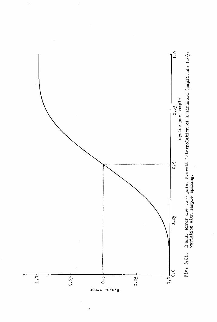
o U\.o .

oJ:OJ:J:8 °S'moH

0 ,....._..--I 0

..--I

Q)'t:1;:s+>.r!r-IASro

'---'

't:1.r!Q) 0r-I Cl)A ;:s

U\ @ I=:I:'- .r!· Cl) Cl)0

!-! roQ)A ct-i

0Cl)Q) I=:r-I 0C) .r!» +>C) Cl!

r-i0

~Q)+>I=:.r!

U\·o

U\N·o

..--IN.C"'I.

0 eo· .r!0 rr..

0.0

o·

't:I·rloIDg·rlID

ctl

~os::o·rl

~r-io~ID.ps::

V'\ ·rl........................................................................ .

o o..--f

V'\. V'\..C\.l o

IDr-i

V'\ i1'- ID·0 f.-!

IDPiIDIDr-i0>..0

o

V'\C\.l·o

·C\.lC\.l·C"'\

0 ·· QO0 ·rl

0 Ii..0

0·00 \J"\ \J"\ \J"\ 0

C"- . N.--l . 0 0

0 0

.IO.I.I8 ·S·III·.I

o

\J"\·o

\J"\N·o

IDrl

\J"\ Po<C"- @0 en

f..IIDPo<enIDrlC}»C}

.C"'IN.C"'I

-68-

4. THREE-DIMENSIONAL PREDICTION WITH PROBE COMPENSATIONUSING A POLARISATION-OVER-AZIMUTH SCANNING DEVICEThe polarisation-over-azimuth scanning geometry is

one which has come very much into favour in recent years for

antenna test facilities, the major reason being that, as

described in Chapter 1 when the geometry was introduced, the

support structure can be kept further away from the front of

the test antenna. It is useful, therefore, to consider the

details of this type of system, in a way similar to that in

Chapter 3 for the elevation-over-azimuth system, with a view

to implementing an iterative procedure for the weighting

function. A further advantage embodied in this type of scan

is that circular symmetry is applicable. In Chapter 3 it was

seen that, as a precursor to the iterative procedure, it was

required to determine the coefficients defining the field

components at each specified point in the plane wave region

due to the probe placed at each of the points of the weighting

function. In the earlier case, this meant the creation of a

separate set of four coefficients for every possible comb ina-

tion of weighting function point and plane wave point (the

factor of four reflecting the need to relate two plane wave

components, E and E , to two probe polarisations). It is. x y

clear from Fig. 4.1 that if the desired plane wave field

distribution is defined in terms of polar components Erpwand Ee ipw

E = sinerpw pw (4.1)

E = coseepw pw (4.2)

(assigning unit amplitude to the plane wave, zero phase to

both components) and the synthesised plane wave is also

y

Erpw

Fig. 4.1. Probe and plane wave for polarisation-over-azimuthgeometry.

y

z

Fig. 4.2. Relationship between probe and plane wave point~for 9w set to zero.

-69-

calculated in this form, then the coefficients relating these

field components at point (rpWI, epWI)' in the plane of

iteration to the probe at point (e ,¢ ) in the weightingWI WIfunction may equally well be used to relate the fields at

(r ,8 + fl8) to the probe at (8 + fie, ¢WI). This meanspWI pWI WIthat it is only necessary to calculate the coefficients relat-

ing the field components at all the plane wave points to the

probe when positioned at those weighting function points lying

along a single radial line. For simplicity, we may consider

the particular radial line to be the line 8w= 0 so that the

situation depicted in Fig. 4.2 is the one to investigate.

4.1 The Coefficients

Let us assume that the probe itself has been charac-

terised on a polarisation-over-azimuth scan system so that,

to determine the probe fields at P (the point rpw' epw) due

to the probe at angular position ¢w (along the line 8w = 0),

it is necessary to formulate the angles 8p and ¢p in the

probe measurement coordinate system corresponding to the

line from the probe to P. From Fig. 4.2, it can be

ascertained that the first of these angles, 8p' is given

by,

(4.3)

and the other, ¢p' by,

¢ = sin- I (Air)p (4.4)

where

(4.5)

-70-

andr =. (rpw·2 + R2 - 2r Rcose sin ~ )~:.. : pw pw 't'w (4.6)

These angular coordinates, Sp and <Pp'enable us to

extract the correct probe field components from the probe

calibration data. It is important to note here that the

coordinate <p , as given above, is that actually used 'inp

the polarisation over azimuth system when the probe pattern

was measured but there is a lateral inversion which means

that the value of e is not quite the e-coordinate used inp

measuring the probe. It is in fact defined by,

e = 7T - ep pm (4. 7)

where e is the e-coordinate relevant to the actual probepmmeasurement system. This should be borne in mind when the

probe field information is included in an implemented system.

The direction of the ep field component, Eep' as used below,

is in the same direction as defined in the probe measurement

system (see Fig. 4.3).

4.1.1 Field Components

Let us determine the X and y components of field

(these are the only components which contribute to Ee andpwE ) due firstly to field component Eep'rpw

E = E sine cos<PwXl ep p

E = -E coseYI ep p

The components due to E<pp are

(4.8)

(4.9)

E == E~ cos excos (B-<P )X2 't'P w (4.10)

y

x

Fig. 4.3. Geometry of the probe measurement system.

z

-71-

Ey2 sin 0:

where0: = sin-1 (sine cos¢)p p

and(3 = sLn"' (sin¢p)

coso:

Equation (4.12) implies that

(4.11)

(4.12)

(4.13)

(4.14)

Combining the above components into Ex and Ey andthen resolving into the desired polar components yields,

E = E cose + E sinerpw x pw y pw

andE = -E sine + E coseepw x pw y pw

whereE = Eep sine cos¢wx p

+ E¢p (cosep cos¢p cos¢ + sin¢ sin¢)w p wand

E = -E cose + EO sine cos¢y ep p ¢p p p

(4.15)

(4.16 )

(4.17)

(4.18)

In the definition of the field components above, thevariation of amplitude and phase due to varying distance,R exp-jk(r-R) has been assumed.

r

4.2 z-OffsetAs in Chapter 3, we now proceed to consider the

effect upon the above of introducing a z-offset, zO' to theplane of iteration. It is not important to modify the speci-

· -72-

fied plane wave distribution as this will merely introduce

a constant phase offset into the predictions which does not

affect the relative phase distribution. The situation is

illustrated in Fig. 4.4.

The distance from the probe to point P is adjusted

from that given in equation (4.6) to read,

r = (rpw2 + R2 - 2R~pw cosepw sin¢w

+ z 2_ 2Rz cos¢)~o 0 w (4.19 )

Equation (4.3) for ep is modified as follows,

e = tan-1p (r cose cos¢w - 20 sin¢w)pw pw

(4.20)

The equation (4.4) for ¢ can remain unaltered,p

(4.21)

but in this case A is modified:

A = (r 2 sin2e +pw pw

(r cose cos~ z sin¢ )2)~pw pw 't'w-:-0 W(4.22)

r is as given in equation (4.22).

Using these modified values of e ,¢ and r, thep p

field components in the plane wave region may be evaluated

as in equations (4.8) to (4.18).

4.3 The Iteration Procedure

The relevant ideas for producing a weighting function,

given the necessary coefficients, are identical to those for

the e1evation-over-azimuth scheme in section 3.3 and need not

be repeated here. It is merely noted that the result is a

weighting function which when applied to measured data at

yp

z

Fig. 4.4. Relationship between probe and plane wave pointwith plane wave z-offset.

-73-

the correct points on the spherical surface and of the

correct polarisations enables a linearly polarised plane wave

of the form of equations (4.1) and (4.2) to be synthesised

in the plane of iteration. By virtue of the depth of field

effects discussed in Chapters 2 and 3, the plane wave field

distribution will, in fact, encompass a volume large enough

to enclose the test antenna positioned at any desired angle.

4.3.1 Timing Difficulties

The procedure used to generate a weighting function,

developed on a polarisation-over-azimuth type of coordinate

system, has been outlined. It was stated early in the

chapter that for the creation of the coefficients used in

weighting function generation, circular symmetry could be

applied to reduce the amount of computer time consumed.

Unfortunately, the same argument does not apply to the

iteration procedure itself since, although the number of

coefficients used is reduced, these coefficients still have

to be applied at all points around the weighting function.

Because of the high density of points around the boresight

pole of the polarisation-over-azimuth system, it was found

that the iteration time was prohibitively increased and so,

although ideas have been considered for some form of data

thinning, it was considered advisable to return to the

elevation-over-azimuth weighting function generation scheme.

4.4 Application of an Elevation-Over-Azimuth Weighting Function

This chapter is concerned with processing of data

obtained with a polarisation-over-azimuth scan system. So

far, we have thus considered a weighting function generated

in the same coordinate system. There is no reason, however,

-74-

why a weighting function generated by the means described

in Chapter 3 cannot be applied to data obtained on a

polarisation-over-azimuth system. It is simply a matter

of generating a composite weighting function using

equations for data selection, interpolation and component

resolution designed for the correct measurement geometry.

4.4.1 Prediction of E¢F

The situation here is illustrated in Fig. 4.5. In

this case, it is convenient to consider the prediction of

the E¢F far-field component along the radial arm eF = 900

(i.e. the centre of the weighting function will move out-

wards from the boresight pole along the radial line e = 900).

We define firstly the angles e and ¢ in the near-field data

set corresponding to the weighting function point (ew' ¢w)

when the function is centred at boresight (¢ = 0) for a

prediction at ¢F = O. These angles are,

(Sinew)e = tan-1tan¢w

(4.23)

(4.24)

These angular coordinates enable the calculation of

the polar field components, Ee and E¢ at the appropriate

point and it is now necessary to resolve these into directions

corresponding to those defined for the weighting function;

+ E~ (cos¢ sine cose + sin¢ sine )~ w w (4.25)

line e = 900

I

Fig. 4.5. Elevation-aver-azimuth weighting function super-imposed upon polarisation-aver-azimuth data sphere.

-75-

and

+ E~ (cosCPcose cosCP - coscp sine sine sin¢~ w w w

+ cose sincp)w w (4.26)

Equations (4.25) and (4.26) enable field components,

which can be used with the weighting function, to be derived,

from those data values produced by interpolation of the

actual measured near-field data. The combination of the

interpolation coefficients, determined on the basis of the

known measurement geometry and the values of e and cp from

equations (4.23) and (4.24), and the component resolution

coefficients of equations (4.25) and (4.26) enables a

composite weighting function to be found for the prediction

at CPF = O. For prediction at any CPF ~ 0, it is merely

necessary to add this value of CPF to the value of ew to be

used in equations (4.23) to (4.26). Such a modification

enables the far-field component ECPF to be evaluated at any

point along the line eF = 900• The circular symmetry of

the data set may be exploited to enable us to say that no

further modifications to equations (4.23) to (4.26) are

needed to produce a prediction at any other angle 8F ~ 900.

It is simply necessary to add the value 8F - 900 to the

value of 8 from equation (4.25) when selecting the near-

field data to be used for the prediction (but the value of

e should be left unchanged for all other purposes).

Before moving over to the prediction of the other

coordinate of the far-field, two points should be noted

with regard to the above. The first of these is that the

-76- .

value of e required in the polar system should be restricted

to anywhere wi thin ± 1800 whereas the· value given in

equation (4.23) will, if implemented directly as given,

produce angles only wi thin the range ± 900 (if the normal

principal value definition applies). In the FORTRAN language,

this can be overcome by use of the ATAN2 function in the form,

ATAN2 (sine cos¢, sin¢ ) which will put the angle e intow w wthe correct quadrant. The second point is that, as usual,

care should be taken that the angles used are not allowed to

go out of the range of the data, and if so then adjustment

of the values of e and/or ¢ is made (as necessary) to bring

the values back within range.

4.4.2 Prediction of EeF

It is convenient for the prediction of the second

far-field component to consider the elevation-over-azimuth-

defined primary weighting function, as formulated in

equations (4.23) to (4.26) (for the boresight prediction),

to be slid off boresight with its centre moving along the

line e = 0 thus producing predictions of EeF for eF = O.

The angular positions assumed by a weighting function point

when the prediction is at ¢F are,

. e'e = tan-1 ( S1n )coset cos¢F + sin¢F/tan¢' (4.27)

and¢ = cos-1 (cos¢'cos¢F - sin¢'cose'sin¢F) (4.28)

where e' and ¢' are the values of e and ¢ resulting from

equations (4.23) and (4.24). It is now necessary to find the

modified equations for the component resolution at that point.

-77-

These are,

+ Ee (cosecose + sinecos¢sine )w w (4.29)

and

- cos¢sinesine sin¢ -cos¢cosesin¢Fcose sin¢w w w w

+ sin¢cos¢Fcose sin¢ )w w+ Ee (-sinecos¢Fcos¢ - cosesine sin¢w w w

+ sinesin¢Fcose sin¢ )w w (4.30)

where e and ¢ are as in equations (4.27) and (4.28)

Again, to produce a far-field prediction at any

other angle eF ~ 0, it is not necessary to modify equations

(4.27) to (4.30) in any way. It is merely necessary to add

eF to the value of e from equation (4.27) when the actual

measured data are being selected for the prediction.

It should be pointed out again that the value of e

from equation (4.27) will, when implemented computationally,

produce the principal value in the range ± 900. To expand

this to the full ± 1800 range it is convenient to examine

the value of e' (which is the result of equation (4.23».

If the sign of e' is the same as that of tan e then the

principal value should be selected. Otherwise the other

possible-quadrant should be used. The usual care should

be taken to modify the angular-coordinates appropriately if

the permissible range is exceeded at any point in the process.

-78-

5. PROBE COMPENSATION EFFECTS AND ERROR ANALYSISIn the earlier chapters of this thesis, the process

of near-field/far-field transformation by plane wave

synthesis has been described and various aspects have been

considered without, in general, a detailed examination of

the errors likely to be involved. When the two-dimensional

experiment (evaluation of a slotted waveguide array) was

described in Chapter 2, some of the practical errors likely

to be present were listed and, in Chapter 3, there was

included a consideration of a number of possible interpola-

tion schemes and the levels of errors which might be

introduced at various sampling rates. In Chapter 6, a

practical prediction will be presented with a discussion of

the particular errors present in that instance. It will be

useful, however, to present a more general investigation of

some of the problems liable to be encountered and in

particular, of errors resulting from the processing and of

the effects of probe compensation. This latter aspect is

looked at in the next section.

5.1 Probe Compensation

Previous chapters have shown how the characteristics

of the measurement probe are incorporated into the procedure

at the stage of generating the weighting function and it has

been pointed out that the probe compensation adds no extra

work to the prediction process itself. In this section,

the effects of the non-inclusion of probe compensation upon

the plane wave are illustrated together with some indication

of the sorts of errors likely to be introduced thereby. In

-79-

addition, a computational simulation is presented of the

prediction of a principal plane cut of the far-field

pattern from an array of dipoles. This provides further

illustration of probe compensation in action.

5.1.1 Effects upon the Synthesised Plane Wave

As an investigation of the effects upon the

synthesised plane wave of incorrect probe compensation,

a weighting function was generated (using the usual

one-dimensional approximation) for the following parameters.

The frequency specified was 10GHz and a 102cm plane wave

was specified initially (69 points at 1.Scm spacing). The

measurement range was chosen to be 2.0m and a weighting

function was generated consisting of 59 points with O.So

spacing. A wide-beam probe (half-power beamwidth of 900)

was assumed.

The weighting function resulting from the iterative

process is shown in Fig. 5.1 with the synthesised plane

wave on the plane z = 0 appearing as Fig. 5.2. Very

uniform amplitude, and phase barely distinguishable from

the zero axis, are features of the plane wave. For the

time being, we pass over Figures 5.3 and 5.4, since the

significance of these will require a little explanation,

and move on to show the effect upon the synthesised plane

wave of using, in the unmodified weighting function, a

probe with a l5ealnwidth different from that for which

the function was designed. In the first case a probe with

a slightly narrower beamwidth. (3dB beamwidth of 750)

is used and the synthesised plane wave is shown as Fig.S.S.

e (degrees)..--. -20 0 20~ 0 180 X X'-" 'X X X X

X XID >$( ..--.'d Cl) xX Xx~ -10 * ID XX XX+'l ID.r!

~ f...l

x,,-x-x~--x-x><-xx.--l bePi

~ID 0@ 'd'-"

'd -20 ~X X

ID XID Cl) X X xXCl) III.r! ..c: X X~ Pi X X~ -30 -1800I=l -20 0 20

e (degrees)

Fig. 5.1. 59-point weighting function designed to synthesise 1.02m.plane wave, at 10.0GHz., using a probe with 90° JdBbeamwidth, at 2.0m. measurement radius.

ID 1.0'd~+'l ..--..r! ID

~~@ g-g ~Cl) ID.r! I=l~ ~ 0.0~'-" -50 0 500I=l Y (cm.)

180..--.

Cl)IDIDf...lbeID 0'd'-"

IDCl)III..c:Pi -180

-50 0 50y (cm.)

Fig. 5.2. Synthesised plane wave due to weighting function ofFig. 5.1, using correct probe.

o "/I

" " "\fu\N

0.60.0sin(e)

Fig. 5.J. Fourier transform of synthesised plane wave shownin Fig. 5.2 (solid) compared with ideal (dotted).

0

-10r---. -20~'--"

Q) -JO'd;::l+.:l -40OMr-ip..El -50<:

-60-0.6 0.0 0.6

sin(e)

Fig. 5.4. Fourier transform of non-ideal residual of plane waveshown in Fig. 5.2 illustrating effective spurious far-field sources.

y (cm.)

Fig. 5.5. Synthesised plane wave due to weighting function ofFig. 5.1 but using probe with 3dB beamwidth of 75°.

o "fI, II

sinCe)Fig. 5.6.

0

-10r--..

~ -20'-""

Q)

'ti -30;j~.r!.-I -40~ex: -50

-60-0.6

Fourier transform of synthesised plane wave shownin Fig. 5.5· (solid) compared with ideal (dotted).

0.0 0.6sinCe)

Fig. 5.7. Fourier transform of non-ideal residual of plane waveshown in Fig. 5.5 illustrating effective spurious far-field sources.

-80-

The phase (not shown) is substantially unaltered by the

use of a different probe but the amplitude is slightly

tapered. A much more drastic taper is introduced, as

illustrated in Fig. 5.8, when a probe with a 3dB beam-

width of only 250 is introduced into the same weighting

function although again, the phase of the plane wave (not

shown) remains virtually unaltered.

Probe compensation can be carried out for the

narrower beam probes and for the case of the medium-beam

probe, the resulting weighting function is shown as Fig.S.ll

with the synthesised plane wave as Fig. 5.12. If the

weighting function is compared with the earlier one (Fig.S.l)

it will be discovered that it is very difficult to detect

any difference between the two. Nevertheless, the slight

improvement in the synthesised plane wave is quite

discernible. For the narrow-beam probe, the weighting

function is shown as Fig. 5.15 with the resulting synthesised

plane wave as Fig. 5.16. The modifications to the weighting

function in this case are noticeable and the removal of the

taper in the plane wave amplitude has been achieved. It

should be noted that it would not prove possible to carry

out probe compensation if the probe pattern had a null in

the region of interest but, of course, it is extremely

unlikely that one would attempt to use such a probe.

5.1.2 Fourier Transform Analysis

We now move on to explain the significance of those

graphs which have been passed-over in the above. The plane

wave synthesis technique, as should now be clear, is

Fig. 5.8.

_..-...-10~

ID -20'ti

E.r!r-Ip.. -30!j

1.0

0.0-50 o 50

y (cm.)

Synthesised plane wave due to weighting function ofFig. 5.1 but using probe with 3dB beamwidth of 25°.

o

....:.t~i.

.'l' f\ IiIi ti!ii\ (\tii\ t,(\1\[\ 1\ i\ i

....

/\ i\ tiM} 11f\{\ Ii [)IiIi11~ !\ ' ,

-40-0.6 0.0 0.6

sinCe)Fig. 5.9. Fourier transform of synthesised plane wave shown

in Fig. 5.8 (solid) compared with ideal (dotted).

_..-...

~ -20

~ -30E.r!r-I -40~ -50

-60-0.6

o ""-10

0.0 0.6sinCe)

Fig. 5.10. Fourier transform of non-ideal residual of plane waveshown in Fig. 508 illustrating high level of effectivespurious far-field sources.

e (degrees)-20 0 20

.,......._ 0 180 X X~ X X X'---' X X.,......._ID m Xx'd ~ ID XX;::s -10 ID+' '*'

H

x"J(-x--A--x~xxo,-! QOr-l

~ID 0

~'d'---'

ctl ID X X-20 >0< X X'd m Xx X X XXID ctlm ..c:: X X X X

O,-! Pir-l X X X Xctl

~ -30 -1800 -20 0 20~

e (degrees)

Fig. 5.11. Weighting function for the same parameters as that ofFig. 5.1 but designed for use with a probe having 75°3dB beamwidth.

o 50y (cm.)

180

IDmctl.cPi -180

-50 o 50y (cm.)

Fig. 5.12. Synthesised plane wave due to weighting function ofFig. 5.11 using correct probe.

o f\..---.-10~

" " n

" '"

0.0 0.6sinCe)

Fig. 5.13. Fourier transform of synthesised plane wave shownin Fig. 5.12 (solid) compared with ideal (dotted).

0

..---. -10~ -20'--'

ID'ti -30E.r!r-I -40~<

-50-60

-0.6 0.0 0.6sinCe)

Fig. 5.14. Fourier transform of non-ideal residual of plane waveshown in Fig. 5.12 illustrating effective spurious far-field sources.

e (degrees)..---... -20 0 20~ 0 180 . X'-"" XXQ)"d )J( ..---... XX;:l

~x UJ+' -10 Q) XX• ..-i

~-~'X-x--~x--x~~x~

r-I X>S<Pi QO

~ X Q) 0"d

"d ~ '-""XQ) -20 Q) X XxUJ XUJ X•r-l cd Xr-I ..ccd Pi

~0 -30 -180,::::

-20 0 20e (degrees)

Fig. 5.15. Weighting function for the same parameters as that ofFig. 5.1 but designed for use with a probe having 25°3dB beamwidth.

o 50y (cm; )

180

Q)UJcd..cPi -180

-50 o 50y (cm.)

Fig. 5.16. Synthesised plane wave due to weighting function ofFig. 5.15 using correct probe.

o -

"

n

-10

-20 -

-30

0.0 0.6sinCe)

Fig. 5.17. Fourier transform of synthesised plane wave shownin Fig. 5.16 (solid) compared with ideal (dotted).

0

-10,......._

f'a -20'---"

ID'd -30~-t-:>OMrl -40~<

-50

-60-0.6 0.0 0.6

sinCe)

Fig. 5.18. Fourier transform of non-ideal residual of plane waveshown in Fig. 5.16 illustrating effective spurious far-field sources.

-81-

dependent upon an attempt to simulate the conditions of

direct far-field measurement by computational manipulation

of the near-field data. When the synthesised plane wave

is examined closely it is seen that it consists in the major

part of the ideal uniform plane wave, which is what would

be produced by the ideal far-field source. In addition,

however, there will be present some deviation from the

perfect plane wave; amplitude or phase ripple, or, as has

been seen above, taper. Such deviations can be thought

of as being the product of interference from other spurious

far-field sources.

The effective far-field source distribution can be

obtained simply by Fourier transforming the synthesised

plane wave distribution. The ideal plane wave component

will appear not as a point-source but, because of the

limited size of the plane wave, as a sinc (sin ae/ae)

function. The other spurious far-field sources will be

present in the form of deviations from this function.

Thus Fig. 5.3 shows the Fourier transform of the synthesised

plane wave of Fig. 5.2. In addition, the Fourier transform

of the ideal plane wave is plotted for comparison as a

dotted curve and in this particular case the two curves

are indistinguishable from one another confirming that the

plane wave is of very good quality.

It is possible to take this reasoning one step

further and to argue that, if the mean value of the

synthesised plane wave is subtracted from all of the plane

wave elements, the residue comprises the results of the

-82-

spurious sources alone. The Fourier transformation will

then yield the positions and sizes of the spurious effective

sources. This process has been carried out for the plane

wave of Fig. 5.2 and the resulting spurious source distribu-

tion is shown as Fig. 5.4. Again, the quality of the

synthesised plane wave is confirmed by the fact that there

are only two very small incursions of the spurious far-

field distribution into the 60dB range displayed. It should

be noted that the full Fourier transform array is displayed

here (the transform was effected by means of an FFT algorithm)

and in certain instances part of the displayed transform will

be for imaginary values of e, i.e. in the invisible region.

In this particular case the edge of the visible region is at

about the point where the spurious source appears in Fig.5.4.

The appearance of a spurious source at a particular angle

means that, as the prediction moves off boresight, the

main beam of the test antenna will pass from the area of

the ideal far-field source through the spurious source so

that the prediction at this angle will consist, in fact of

the required far-field prediction plus the main beam

distribution of the pattern attenuated by whatever is the

level of the spurious source below OdB. The occurrence ofothe spurious sources in the above example at e ~ ±90 and at

a level of almost -60dB indicates that the pattern prediction

at e ~ ±900 will be subject to a-possible error equivalentF

to 60dB below the main beam (assuming that the test antenna

is aligned with its main beam at the zero angular coordinate.

A similar Fourier transformation analysis was

carried out for the case of the medium-beam probe, the two

-83-

diagrams forming Figs. 5.6 and 5.7. Again, very little

deviation of the plane wave Fourier transform from the

ideal are visible but in this case, the Fourier transform

of the residual after subtraction of the ideal plane wave

indicates the appearance of two further spurious effective

sources at e ~ ±So and at a level of about -SOdB. In this

case, therefore, the worst effects of the non-ideal quality

of the synthesised plane wave would appear a few degrees

either side of boresight.

For the narrow-beam probe, the Fourier transform of

the synthesised plane wave (Fig. 5.9) shows considerable

differences from the ideal and this is reflected in Fig.S.lO

showing the Fourier transform of the non-ideal residue. In

this case, the spurious far-field sources reach a level of

-20dB confirming the unacceptability of this plane wave

taper for most practical purposes.

After probe compensation for the medium-beam probe

(as appeared in Fig. 5.12) the taper was removed from the

synthesised plane wave and Figs. 5.13 and 5.14 confirm

that the spurious far-field source level has once more

been reduced to almost -60dB. On the other hand, the

narrow-beam probe proves a more difficult case to correct

since the probe-compensated plane wave (as seen in Fig.

5.16) still has some residual ripple and although its

Fourier transform differs from the ideal apparently in only

minor Wqys (Fig. 5.17), the spurious source distribution

revealed when the non-ideal residual is transformed (Fig.

5.18) doe's extend above the -SOdB mark. More iterations

(in this case the iteration was terminated after 45)

would probably effect some additional improvement.

-84-

5.1.3 A Simulation

An. array of vertically polarised half-wave dipoles

was modelled computationally as a further investigation

of probe compensation in action. A frequency of 10GHz

was used and the array was specified to be 11 elements

wide by 21 elements high with A/2 spacing in both directions.

"Measured" near-field data were computed over a band of 13

points, angular spacing 3.60, extending along the elevation

(E-plane) principal axis at a range of 1.Om. Only one

polarisation of data was used. From these simulated near-

field measurements a principal plane pattern was predictedo(over a 90 range, symmetry applying for the other quadrants).

The true far-field was evaluated analytically and used as a

comparison for the prediction.

In Fig. 5.19 is shown a comparison of the prediction

of the far-field pattern using a probe with a cosinusoidal

main beam, 3dB beam width of 900, and the true far-field.

Good accuracy is observed over most of the pattern down to

the -60dB level. Using the same weighting function, a

prediction was performed using the data which would be

measured with a probe having only a 120 3dB beamwidth and

the prediction is compared with the true far-field in Fig.

5.20. A significant lowering of the predicted sidelobe

levels together with shifting of the nulls is apparent.

When probe compensation for the directive probe was

performed the predicted pattern changed to that shown in

Fig. 5.21 (compared again with the true far-field).

Virtually all of the pattern shows a marked improvement

over the uncompensated case. Errors are still present in

0

-10

-20,,---._

~<:»

Q) -]0rd;:j+l.,-lr-l

t -40

-50

-6090 45 0

e (degrees)Fig. 5.19. Far-field pattern (over one quadrant - symmetry applies)

of dipole array. E-plane cut predicted using wide-beamprobe (solid) compared with true pattern (dashed).

Or-------------------------------------------------------_

-20,,---._

~..__,Q) -]0rd

E.,-lr-I

~-40

-50

-6090

-101

~I'\I'",,

I•

I

1I,I

e (degrees)o

Fig. 5.20. Far-field pattern of dipole array. E-plane cutpredicted using narrow beam probe, uncompensated(solid) compared with true pattern (dashed).

o r-----------------------------------------~

-10

r--.. -20~.........Q)

-30'd~~.r!r-l

~ -40

-50

-6090 45 o

e (degrees)

Fig. 5.21. Far-field pattern of dipole array. E-plane cutpredicted using narrow-beam probe, compensated(solid) compared with true pattern (dashed).

-85-

places but it will be realised that this is a far more

directive probe than is likely to be used in a practical

measurement system. It should also be noted that this

simulation indicates that it is possible to obtain useful

results using only one polarisation of near-field data

given the right circumstances although, in general, both

polarisations of the near-field will be required.

5.2 Effects of Measurement Errors

A useful summary of some of the types of errors

liable to be found in a practical measurement system is

given by Joy (32) Although this is intended to apply

particularly to the planar scan geometry, most of the errors

are applicable to any measurement system. A brief analysis

has been carried out of the sorts of effects which these

errors might introduce and certain other effects, also.

This is mentioned in section 5.2.2. Firstly an investigation

of a particular type of random noise introduction is

presented.

5.2.1 Level-Independent Random Noise

The effect of random noise in the measured near-field

data when multiplied by the weighting function can be

thought of as essentially similar to ideal data being

processed by a weighting function containing random errors.

In this particular investigation, normally distributed

random noise of a specified amplitude standard deviation,

random phase, was introduced into the weighting function

and the resulting errors in the plane wave and its Fourier

transforms were observed. There was no attempt to link this

-86-

to a particular set of near-field data but the noise

values were multiplied by the appropriate weighting function

element before being added to it (i.e. the noise was

weighted in the same way as would be done with the actual

measured data). The reasoning behind this might be

thought of as follows. As the test antenna is scanned,

its main beam region will pass around the walls of the

anechoic chamber (assuming that the measurement is taking

place within such a chamber). There will be some reflections

which will appear as noise at a certain level within the

data and will thus be weighted along with the desired data.

Thus the weighted noise will appear as the unwanted ripple

superimposed upon the synthesised plane wave. A similar

argument can be applied for any random noise appearing in

the data (such as receiver noise, etc.)

In this test a 50cm plane wave was specified at

lOGHz with a measurement range of 1.Om. A 29-point (one-

dimensional) weighting function was used with 2.50 spacing.

The synthesised plane wave with its Fourier transform and

the transform of the non-ideal residual are shown in Figs.

5.22, 5.23 and 5.24. Very little deviation from the ideal

is detectable in the synthesised plane wave and Fig.5.24

shows that the effective spurious far-field sources are at

a level of better than -70dB. If noise is introduced at

a standard deviation of -40dB into the data, the effective

synthesi.sed plane wave begins to show a little ripple

(Fig. 5.25) and although little discrepancy is visible,

in Fig. 5.26, between the Fourier transform of the plane

wave and that of the ideal, a spurious far-field effective

Q) 1.0'0::J-j-l""""".,-j Q)MMPimS 0m Ul'OHQ) mUl Q).,-j ~M .,-jmM~'-'0 0.0~ -20 -10 0 10 20

y (cm. )

180

,......."

UlQ)Q)Htill 0Q)'0'-'

Q)Ulm..c:Pi-180

-20 -10 0 10 20y (cm. )

Fig. 5.22. Synthesised plane wave due to 29-point weighting functionwith no introduced noise.

0

'""' -10~"'--"

ID -20't:l~->.r-!r-iPI -30s<

-40-1.0 0.0 1.0

sinee)

Fig. 5.23. Fourier transform of synthesised plane wave shown inFig. 5.22 (solid) compared with ideal (dotted).

0-10

'""' -20~'-../ -30ID't:l -40~+".r-! -50r-i§' -60<

-70-80

-1.0 0.0 1.0sinee)

Fig. 5.24. Fourier transform of non-ideal residue of synthesisedplane wave shown in Fig. 5.22.

ID 1.0'd;::s+' .---....r-! IDrlrlp..cUS ()cU U)

'd ~Q) cUU) ID.r-! s::rl .r-!cUrl~'--'0s:: 0.0

-20 -10 0 10 20

Y (cm.)

180.---...U)Q)

~bOID'd 0'--'

Q)U)cU..c:p..

-180-20 -10 0 10 20

Y (cm.)

Fig. 5.25. Synthesised plane wave due to 29-point weighting functionwith normally distributed random noise added at a levelof -40dB.

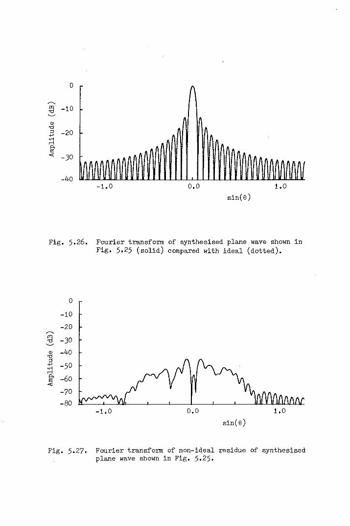
IDrc:JE -20.r!rl

~<

o

-JO

.-40-1.0 0.0 1.0

sinCe)

Fig. 5.26. Fourier transform of synthesised plane wave shown inFig. 5.25 (solid) compared with ideal (dotted).

0-10-20,......,

~ -JO'--'"

ID -40rc:J::J

-f-.:l -50.r!rl

~ -60<

-70-80

-1.0 0.0 1.0sinCe)

Fig. 5.27. Fourier transform of non-ideal residue of synthesisedplane wave shown in Fig. 5.25.

-87-

source level of about -45dB is apparent in Fig. 5.27.

When the noise level is increased to -30dB, the

synthesised plane wave, displayed in Fig. 5.28, has a

Fourier transform (Fig. 5.29) which possesses considerably

more deviation from the ideal and the spurious far-field

source level (Fig. 5.30) has risen to above -35dB.

Continuing the trend, if the measured noise level is

increased to -20dB, the synthesised plane wave (Fig.5.3l)

exhibits severe ripple, its Fourier transform (Fig. 5.32)

now deviates markedly from the ideal and the spurious far-

field source distribution (Fig. 5.33) has risen by another

10dB. Clearly this latter case would be of little value

for measuring any antenna but the earlier cases (-30dB

and particularly -40dB noise) might be usable in the right

circumstances dependent upon the antenna being measured

and the accuracy required.

5.2.2 Non-Ideal Probe

It may be the case that the dual polarised probe

(assuming that such a device is in use) does not possess

perfect orthogonality of polarisation. A technique for

extracting correctly polarised data from a non-ideal probe

has been formulated by Bach et al (33) and this technique

can be used to correct for this type of error.

5.2.3 Other Measurement Errors

Under this heading are included the other types of

error which might occur on the R.F. side of the system,

but we do not cover the various mechanical errors which

can occur. These will be mentioned shortly. A number of

simulations have been performed (34), using a scalar approach,

(]) 1.0'"Cl;j.p ,.-....·rl (])....-f....-fPi cO@ g'"Cl f.-l(]) cOrf.l (])·rl ~....-f -r-icO....-f~'-/

0~ 0.0

-20 -10 0 10 20y (cm. )

180,.-....rf.l(])(])f.-lQD(])'"Cl 0'-/

(])rf.lcO.cPi

-180-20 -10 0 10 20

y (cm. )

Fig. 5.28. Synthesised plane wave due to 29-point weighting functionwith normally distributed random noise added at a levelof -30dB.

o

-10

~ -20;::!->.r!rl

~ -JO<

-40-1.0 0.0 1.0

sine e)

Fig. 5.29. Fourier transform of synthesised plane wave shown inFig. 5.28 (solid) compared with ideal (dotted).

0-10

,.-.... -20~~'---" -JOID"d -40E.r! -50rl

~ -60<-70-80

-1.0 0.0 1.0sinCe)

Fig. 5.JO. Fourier transform of non-ideal residue of synthesisedplane wave shown in Fig. 5.28.

Q) 1.0'Cl~.p _...-....-r-i Q)rlrlPiro~ ~'Cl 1--1Q) ro[I) Q)·rl s::rl ·rlrorl~'-/

0s:: 0.0

-20 -10 0 10 20y (cm. )

180_...-....[I)(J)Q)1--1QOQ)'Cl 0 -------'-/

(J)[I)ro..c:Pi

-180-20 -10 0 10 20

y (cm. )

Fig. 5.31. Synthesised plane wave due to 29-point weighting functionwith normally distributed random noise added at a levelof -20dB.

o

Q)'d

E.r-!rl

~ -JO<

-20

..--...-10~

-1.0 0.0 1.0sinCe)

Fig. 5.J2. Fourier transform of synthesised plane wave shown inFig. 5.Jl (solid) compared with ideal (dotted).

0-10

..--... -26~ -JO<::»

Q) -40'd::s+> -50.r-!rl

~ -60<-70-80

-1.0 0.0 1.0sinCe)

Fig. 5.JJ. Fourier transform of non-ideal residue of synthesisedplane wave shown in Fig. 5.Jl.

-88-

of various measurement errors which can occur in a

practical system and the results are summarised briefly

here.

The simulation was of an X-band lOA antenna and one

of the investigations involved uniform illumination of

the antenna and simultaneous introduction of the errors

numbered 1 to 10 of those listed by Joy (32) at the levels

suggested as the maximum allowable. The most noticeable

effect due to the presence of the errors was a change in

the level of some of the sidelobes, for instance an error

of 0.5dB in a sidelobe at -27dB. When the errors introduced

were increased by a factor of 5, the resulting errors in

the prediction were much more severe with the 0.5dB error

now appearing in the first (-12dB) sidelobes. Inner nulls

were filled to about -35dB and some null positions wereoshifted by up to 0.5. Similar results were observed when

the above errors (not multiplied by 5) were introduced

into the near-field of an antenna with a tapered illumination.

When the antenna was illuminated in a monopulse configuration,

rather more significant errors were observed, typically

IdB at -25dB.

The other type of error investigated was quantisation

error. Near-field phase quantisation was tried at 100

intervals, 300 intervals and 600 intervals. The 100

quantisation introduced little discernible error. Under

300 quantisation some error was observable, perhaps 0.4dB

in the first sidelobes and some filling of inner nulls. The

600 quantisation introduced much greater error, almost 1.5dB

in the first sidelobe, filled inner nulls (to -25dB) and

-89-

null shifts of up to about 10. The amplitude quantisation

was at 100 levels, linear. The errors produced in this

latter case were of similar magnitude to those due to the

errors from Joy (0.5dB at -27dB).

5.2.4 Mechanical Errors

A useful investigation of the d~fferent types of

mechanical errors likely to be present in a spherical near-

field measurement system is given by Jensen (35) and it is

believed that the effects due to a prediction by the plane

wave synthesis technique will be broadly similar. The

general effects of some types of error are listed below.

These are discussed as they apply to a polarisation-over-

azimuth system. Clearly the application to another type

of scanning system will in some cases be different.

(a) Probe position. Position error as regards the

azimuth direction of the scanning system will be equivalent

to an error in the setting up of the azimuth zero position

and will be discussed under that heading. It will be shown

later in this chapter that measurement distance error and

frequency error are to some extent equivalent and so that

too is covered no further here. The remaining inaccuracy

possible is that the height of the probe will not be the

same as the height of the centre of rotation. The result

of this will be, as shown in Fig. 5.34, that the fields

are measured around scans at slightly incorrect ¢ values

(the dLs'c.repancy decreasing as ¢ increases to become zero

at ¢ = 900), slightly incorrect 8 values (again decreasing

as ¢ increases to a minimum of tan-1 (h/R) where h is

the probe height error) and at these angles the polarisation

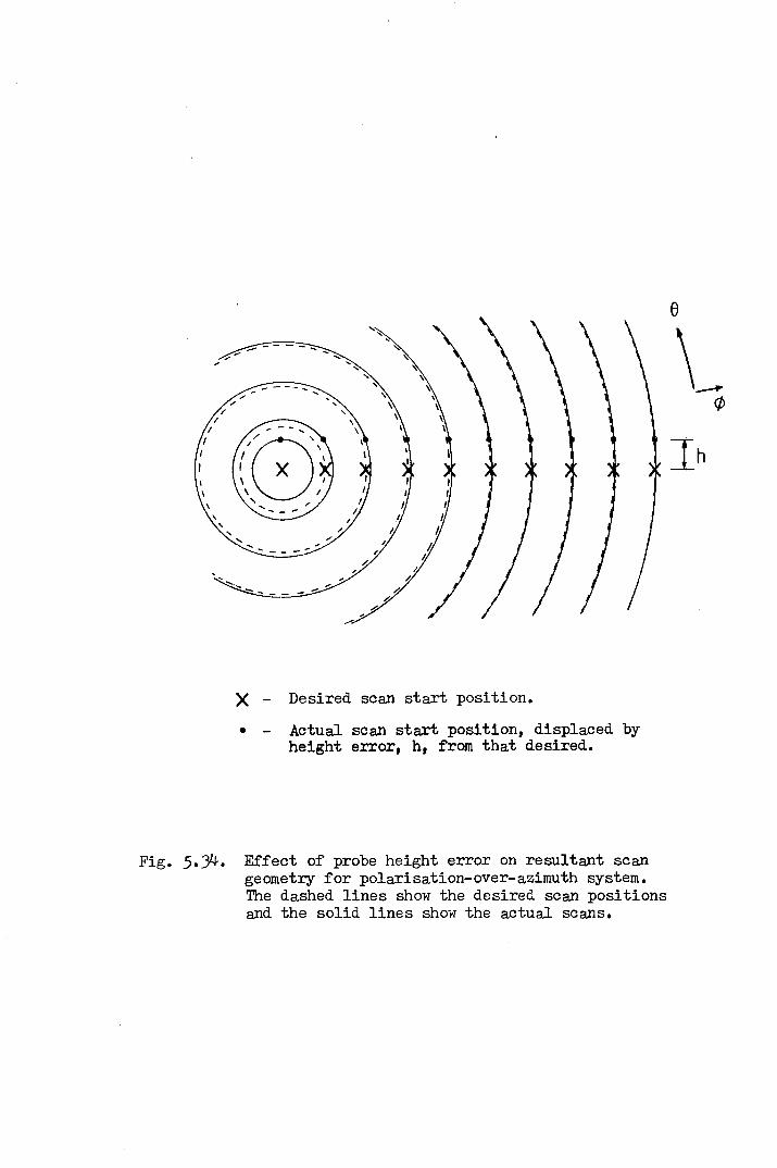
e

\_et>

x - Desired scan start position.• Actual scan start position, displaced by

height error, h, from that desired.

Fig. 5.34. Effect of probe height error on resultant scangeometry for polarisation-over-azimuth system.The dashed lines show the desired scan positionsand the solid lines show the actual scans.

-90-

will not be quite accurate.

(b) Probe pointing. If the pointing of the probe is not

correct the effect will be as if a slightly incorrect probe

had been used. Section 5.1 may be consulted for further

demonstration of the possible effects.

(c) Probe polarisation. This will be particularly

relevant where cross-polar patterns are being predicted.

If the polarisation is not correct then a small amount

(proportional to sin ~ where ~ is the polarisation error)

of the co-polar will appear also.

(d) Azimuth axis verticality. If the azimuth axis is

not truly vertical the polarisation axis, although it may

start horizontal, will not remain so and therefore effects

similar to probe height error will appear.

(e) Polarisation positioner axis horizontality. Again

the effects will be broadly similar to probe height

error.

(f) Intersection of positioner axes. If the axes of

the two positioners do not intersect accurately the

measurement surface will not be a sphere (as shown in

Fig. S.35) but will in fact be the surface of rotation

created by rotation of a circular arc which is not half

of the desired circle.

(g) Azimuth zero setting.

will add a constant ¢ error.

An error in this setting

One pole of the data set

(boresight or rear boresight) will be omitted from the

scan while the other will be overlapped.

(h) Sample position errors. There will be small over-

shoots on the positions at which data are taken. In the

system used at the University of Sheffield antenna test

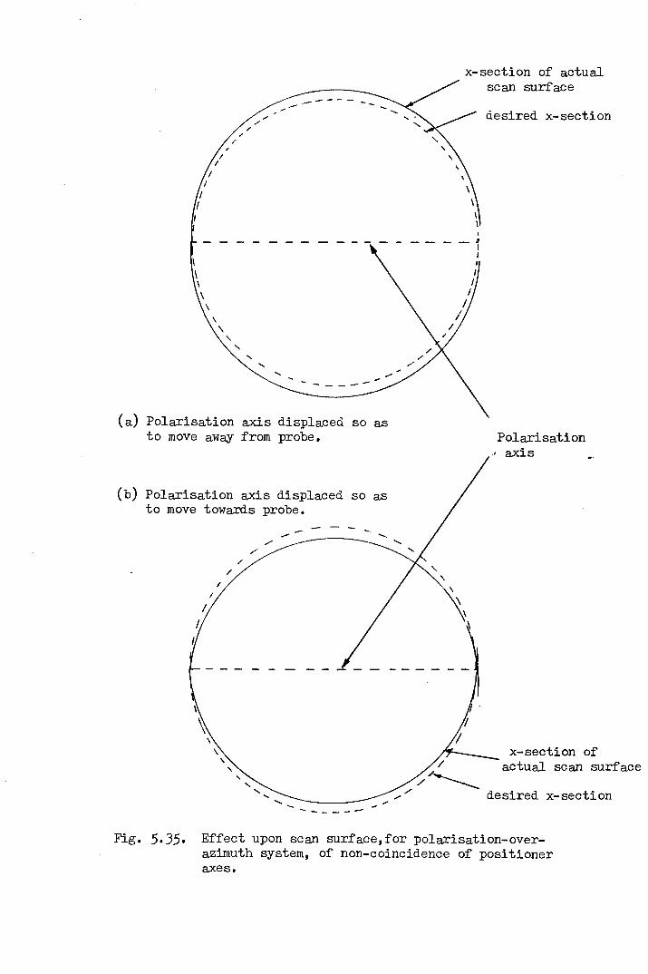
x-section of actualscan surface

desired x-section

.....

,- ~

II

\\\\\\\,

-,.....

(a) Polarisation axis displaced so asto move away from probe.

(b) Polarisation axis displaced so asto move towards probe.

Polarisation, axis

"/

/

I

\~

///....____",,..

x-section ofactual scan surface

desired x-section------

Fig. 5.35. Effect upon scan surface,for polarisation-over-azimuth system, of non-coincidence of positioneraxes.

-91-

site the scans of data are taken in polarisation and

between scans, the azimuth incrementation is performed

relatively slowly so that the error in this latter

coordinate should be slight. In the polarisation

coordinate (8), there will be some error introduced by

the finite sample time and this will appear as a slight

offset in 8F of the prediction direction. There will, of

course, be a slight smearing effect over the integration

time and, if the sample interval is not an exact multipleoof 0.01 (the resolution of the equipment being used)

there will be a small quantisation error. Of course, if

the angular indication from the equipment is not accurate

then this will be an additional error.

5.3 Weighting Function Edge Effects

In a way similar to that encountered with the

compact range (36), it is found that one of the most serious

sources of ripple in the synthesised plane wave is due to

the discontinuity found at the edge of the near-field

weighting function. This is displayed clearly by the

three graphs comprising Fig. 5.36. These consist of the

synthesised plane wave (amplitude only), its Fourier trans-

form and the transform of the ripple component of the plane

wave (the spurious far-field source distribution) due to

a 17-point weighting function, angular spacing 30, at a

measurement range of 1.Om. The frequency used was 10GHz.

The synthesised plane wave has a substantial amount of

ripple. This diagram corresponds to the "first guess"

weighting function before any iteration and was chosen

specifically for its large ripple component. The

....... ...... . ... ....-10 o 10

(a) y (cm.)

o

-30

-40 ~AIII ~I 'IIIIIMN

~~ -10

-20

-1.0 0.0 1.0sin(e)(b)

0

-10

~ -20~..........ID -30'd

E -40.,...,,..;

t -50

-60

(c)Fig. 5.36.

-1.0 0.0 1.0sin( e)

(a) 30em. synthesised plane wave amplitude (solid) withamplitude of non-ideal residue shown as dotted. First guess,before iteration. (b) Fourier transform of plane wave(solid) compared with ideal (dotted). (c) Fourier transformof non-ideal residue of plane wave.

-92-

amplitude of the ripple component of the plane wave is

shown as the dotted line on this graph. The Fourier trans-

form shows its worst deviations from the ideal in the

fourth side lobe and this is even more apparent in the graph

showing the Fourier transform of the non-ideal parts of the

plane wave. The peak values of the spurious far-field

sources appear just outside the x-axis scale-ticks corres-

ponding to sin-1 0.4 (which is 23.50) and from the figures

above it may be realised that the weighting function

extends to ±24° thus the source of the ripple in the

synthesised plane wave corresponds exactly with the edge

of the weighting function. The peak level of the spurious

effective far-field sources is at -35dB.

After two cycles of the iterative procedure the

ripple in the synthesised plane wave has visibly reduced

and this is confirmed by the fact that the spurious far-

field sources have reduced to -42dB, this being displayed

in Fig. 5.37. Another three iterations see the spurious

source level down to -45dB (Fig. 5.38). By iteration 30,

the spurious far-field source level has fallen to -5ldB

(Fig. 5.39) and the reduction in the ripple continues so

that finally by iteration 80 the peak level is at -63dB

(Fig.5.40).

It appears from this that under certain circumstances,

edge discontinuity of the weighting functions can be the

principa~ source of synthesised plane wave deviation from

the ideal. The application of the usual iterative process

reduces the ripple (and the corresponding spurious effective

far-field source level). In a relatively coarsely sampled

,.........,~ -10Q)'"dE -20·rlrl~< -JO

-40(b)

,.........,

~ -20Q)'"dE -JO·rlrl~ -40<

(c)

Q) 1.0'"d:::1'+',.........,·rl Q)rlrlPiroEl oro UJ

'"df...!Q) roUJ Q)·rl 5::rl ·rlrorl~'--'0 0.05::

-10 0 10(a) y (cm.)

o

-1.0 0.0 1.0sinee)

o

-10

-50-60

-1.0 0.0 1.0sinCe)

Fig. 5.J7. (a) Jacm. synthesised plane wave amplitude (solid) withamplitude of non-ideal residue shown as dotted. Beforeiteration J. (b) Fourier transform of plane wave (solid)compared with ideal (dotted). (c) Fourier transform ofnon-ideal residue of plane wave.

-10 o 10y (cm.)(a)

o

~ -10

Q)

'd -20;::l+>•.-1rlPi!Z -JO

-40-1.0 0.0 1.0

sinCe)(b)

o

Q)

'g -JO+>•.-1rl~ -40<

-10~~ -20

-50

-1.0 0.0 1.0sinee)(c)

Fig. 5.J8. (a) Jacm. synthesised plane wave amplitude (solid) withamplitude of non-ideal residue shown as dotted. Beforeiteration 6. (b) Fourier transform of plane wave (solid)compared with ideal (dotted). (c) Fourier transform ofnon-ideal residue of plane wave.

~ -10'--'

(b)

'-../ -20Q)rcJ

.E -JO.r!rl

~« -40

-60(c)

-10 o 10(a)

o

"1\

-JO -

-40 ~IIIHU~ I

-1.0 0.0 1.0sinCe)

o

-10

-50

-1.0 0.0 1.0sinCe)

Fig. 5.J9. (a) JOcm. synthesised plane wave amplitude (solid) withamplitude of non-ideal residue shown as dotted. Beforeiteration JO. (b) Fourier transform of plana wave (solid)compared with ideal (dotted). (c) Fourier transform ofnon-ideal residue of plane waye.

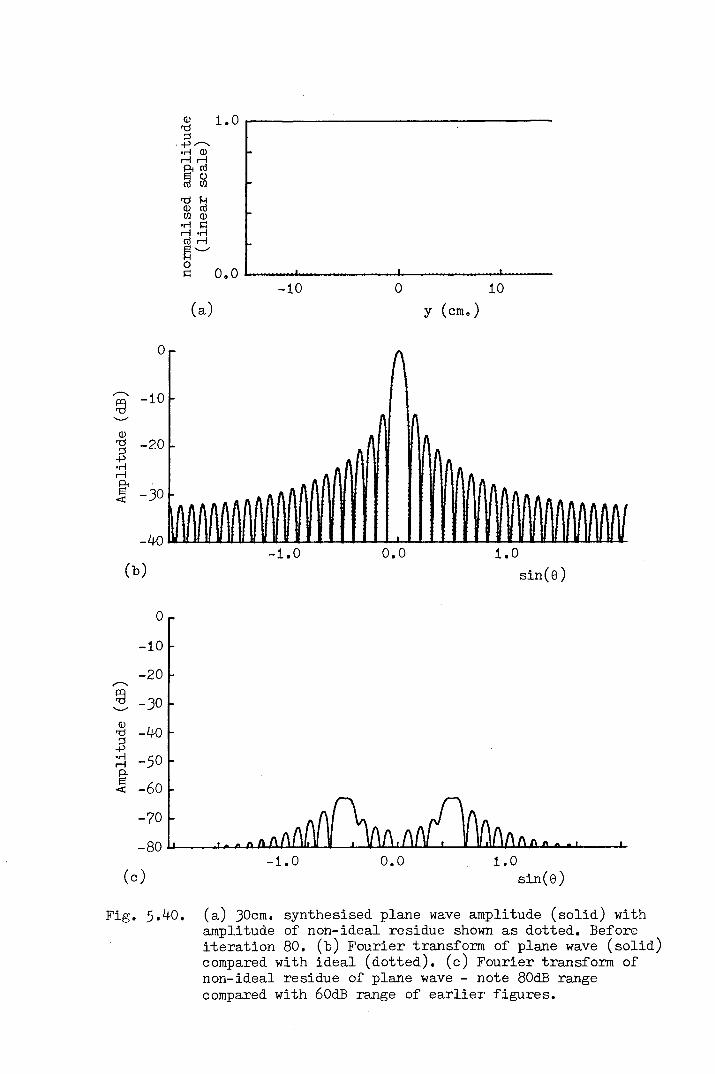
-10 o 10(a)

o

-JO II ~ It ~

-40 ~~A..IL.II-f,t~ul.--a--IL.-&.-&~.I--£....l-I-I~"""""""'a...a.....&.-a-~"""'-&-\N

II

-1.0 0.0 1.0sinee)

0-10-20

"......,.

~ -JO'-"

ID -40'd;::!->.r! -50r-I

~ -60«

-70-80

(c)

Fig. 5.40.

-1.0 0.0 1.0sinCe)

(a) JOcm. synthesised plane wave amplitude (solid) withamplitude of non-ideal residue shown as dotted. Beforeiteration 80. (b) Fourier transform of plane wave (solid)compared with ideal (dotted). (c) Fourier transform ofnon-ideal residue of plane wave - note 80dB rangecompared with 60dB range of earlier figures.

-93-

weighting function, it is believed that the convergence

of the iteration towards the optimum weighting function

will be slower because of the relatively fewer degrees of

freedom available for removing the edge effects.

5.4 Frequency Tolerance of the Weighting Function

The synthesised plane wave, over 50cm, due to a

29-point weighting function, spacing 2.50, measurement

range 1.Om, frequency lOGHz, has already been shown as

Fig. 5.22. The weighting function is, however, not

restricted to use at exactly the frequency for which it

was designed. To determine the frequency band over which

the weighting function might be usable, the plane wave was

examined with the same weighting function used at a range

of frequencies. The different frequencies together with a

summary of the effects upon the synthesised plane wave are

as follows:

(a) 9.5GHz (Fig. 5.41)

Little effect on plane wave amplitude but a slight

phase curvature is introduced.

(b) 9.5GHz (Fig. 5.42)

Effects as for (a) but slightly more pronounced.

(c) 9 •OGH z (Fig. 5.43)

Still little effect on plane wave amplitude but

greater phase curvature.

(d) lO·.2GHz (Fig. 5.44)

Effects of a similar order to those in (a) but

inverted phase curvature.

-20 -10 o 10y (cm.)

20

180r--,.

CI.lQ)Q)f..leoQ)'d 0..__..Q)UJIII.cPi

-180-20 -10 0 10 20

y (cm. )

Fig~ 5.41. Synthesised plane wave due to 29-point weightingfunction (as Fig. 5022) but at the incorrect frequencyof 9.8GHz.

-20 -10 o 10

Y (cm.)

20

180_......_(J)ID

~eoIDrcj 0'--' -----------ID(J)ro.c::Pi

-180-20 -10 o 10 20

y (cm.)

Fig. 5.42. Synthesised plane wave due to 29-point weightingfunction but at the incorrect frequency of 9.5GHz.

ID 1.0'd;:)~r-..or-! ID

~~@ ~'g ~U) ID

or-! s::~~~'--'0 0.0s::

-20 -10 0 10 20y (cm.)

180r-..U)ID

~eoID'd 0'--'

IDU)ro.cPI

-180-20 -10 o 10 20

Y (cm; )

Fig. 5.43. Synthesised plane wave due to 29-point weightingfunction but at the incorrect frequency of 9.0GHz.

-20 -10 o 10y (cm.)

20

180..----..(J)Q)Q)

!-leoQ)

rtJ'--' 0

Q)(J)cd..c:PI

-180-20 -10 0 10 20

y (cm. )

Fig. 5.44. Synthesised plane wave due to 29-point weightingfunction but at the incorrect frequency of 10.2GHz.

-94-

(e) lO.5GHz (Fig. 5.45)

In~reased phase curvature.

(f) 11.OGHz (Fig. 5.46)

Effects more severe than (e) and the phase curvature

is slightly greater than observed in (c).

The classical Rayleigh range (2D2/A) criterion for

far-field measurement is defined as the distance at which

the edge phase taper reaches 22.50 for a boresight

measurement. It is possible to calculate an equivalent

measurement range for the edge phase taper in each of the

above cases and this can then be compared with the Rayleigh

range. The edge phase tapers and equivalent measurement

ranges in each case are listed in Table 5.1. From examina-

tion of these values and comparison with the Rayleigh range

of 16.8m, it may be concluded that the same weighting

function may be used over a frequency range of approximately

IGHz yielding a synthesised plane wave at least as good as

(and generally considerably better than) that produced by

a point source radiator at the Rayleigh range.

5.5 Range/Wavelength Scaling

It is possible to extend the range of usage of a

given weighting function by scaling all the linear dimensions

(measurement range, width of synthesised plane wave, etc.)

in proportion to the wavelength. This is easy to demonstrate

graphically. The synthesised plane wave as shown in Fig.5.22

is displayed on a wider scale in Fig. 5.47. When the

frequency (alone) was altered to 12.5GHz, as shown in

Fig. 5.48, the phase, in particular, of the plane wave

-20 -10 o 10Y (cm.)

20

180,.--...I/JID

~bDIDre! 0'--" -----------IDI/Jro..c:Pc

-180-20 -10 o 10 20

y (cm; )

Fig. 5.45. Synthesised plane wave due to 29-point weightingfunction but at the incorrect frequency of 10.5GHz.

ID 1.0""t:j~+> r--.OM ID

~~@ ~-g ~Cf.l IDOM ~~;:I~~0~ 0.0

-20 -10 0 10 20y (cm. )

180r--.

Cf.lIDID!-lQOID""t:j 0<:»

ID

~.cP<

-180-20 -10 o 10 20

y (cm.)

Fig. 5.46. Synthesised plane wave due to 29-point weightingfunction but at the incorrect frequency of 11.0GHz.

Table 5.1

Edge phase taper and equivalent measurementrange for plane wave due to weighting

function used at a range of frequencies

f(GHz) Edge phase Equivalent Rtaper (degrees)

9.0 36.0 10.4m9.5 19.5 19.2m9.8 6.0 62.Sm

10.0 0.0 bo

10.2 10.5 3S.7m10.5 25.5 l4.7m11.0 48.0 7.8m

y (cmv)

180.........

Cl}Q)Q)f..!eoQ)'d 0'-'"

Q)Cl}cO.cPi

-180-50 0 50y (cm.)

Fig. 5.47. Synthesised plane wave due to 29~point weightingfunction (as Fig. 5.22 but displayed over a widerarea) •

y (cn; )

180_........tf.lIDIDf..feoID'l:l 0.........IDtf.lro.cPI

-180-50 0 50

y (cm.)

Fig. 5.48. Synthesised plane wave due to 29-point weightingfunction but at the incorrect frequency of 12.5GHz.

-95-

acquired a pronounced curvature. By scaling down the

measurement range to 80cm, the plane wave quality, shown

in Fig. 5.49, was restored (the change in amplitude and

the phase offset are merely due to the way the probe was

initially defined and to the fact that no new normalisation

was carried out). As an extreme example, the frequency was

changed to 20GHz and Fig. 5.50 indicates that the plane wave

had broken down badly particularly in phase. A reduction

of the measurement range to 50cm, however, restored the

plane wave quality over, now, a 25cm area (Fig. 5.5l).

Lastly the frequency was reduced to 5GHz whereupon the

synthesised plane wave was seen to exhibit a significant

taper and, again, phase breakdown (Fig. 5.52) but a move

to 2m measurement range once again restored the quality

(Fig. 5.53).

It should be noted that the above scaling process

depends on the characteristics of the measurement probe

not altering in any significant way under the frequency

change. Certain types of probe, for instance some scalar

feeds, have the useful property of not changing their

radiation patterns over restricted frequency ranges so

that this mi"ght be feasible in such a case. Otherwise, a

practical measurement facility might consider having a

number of scale-model probes for use at different

frequencies but, whatever the method used, the end result

must be the maintenance of the probe's radiation character-

istics. If this can be achieved then there is no theoretical

reason why the bandwidth of a given weighting function cannot

be regarded as effectively infinite.

1.0

0.0-50 o 50

y (cm.)

180""If.lQ)Q)~b.OQ)'d 0'-"

Q)If.lIII

-&

-180 I

-50

~ -- ------------------------------------ - ~~1~~1~~

~ .•. U ,o 50

y (cm.)

Fig. 5.49. Synthesised plane wave due to 29-point weightingfunction at the incorrect frequency of 1205GHz.but with the measurement radius scaled inproportion to A (to 80cm.).

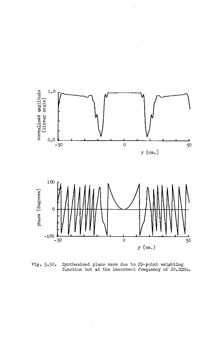
180........II.lIDID~eoIDrd 0'-"

IDII.lttl..cPi

-180-50

1.0

0.0 ~--~--~--_'--~~ __ ~ __ ~ __ ~ __ -L __ ~ __ ~

-50 o 50y (cm.)

~~ ~ \I

!--ooj - - -- -- - - - - - --

V-II \-• • . • • • •

o 50y (cm. )

Fig. 5.50. Synthesised plane wave due to 29-point weightingfunction but at the incorrect frequency of 20.0GHz.

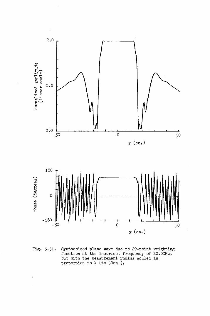
2.0

1.0

0.0-50 o 50

y (cm.)

180........_

Cl)IDID~tillID'Cl 0'-"ID

~-&

-180 I

-50

I \

tHi'+H·f+H+t~H·U·tH·.+H~"'i+----------------------H-"""'HotIH"'(of"HiI+Hn~H""H

• • •o 50

y (cm.)

Fig. 5.51. Synthesised plane wave due to 29-point weightingfunction at the incorrect frequency of 20.0GHz.but with the measurement radius scaled inproportion to A (to 50cm.).

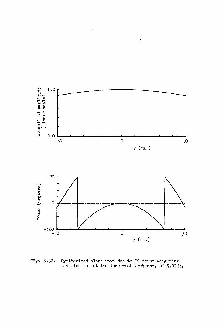
(J) 1.0'"(j;j~~·H (J)

r;tr-;;!@ g~ ~ff.l (J)·H I=lr-;;!~t:l~0I=l 0.0

-50 0 50y (cm.)

180~ff.l(J)(J)~eo(J)'"(j 0~(J)tnet!.cPi

-180-50 0 50

y (cm. )

Fig. 5.52. Synthesised plane wave due to 29-point weightingfunction but at the incorrect frequency of 5.0GHzo

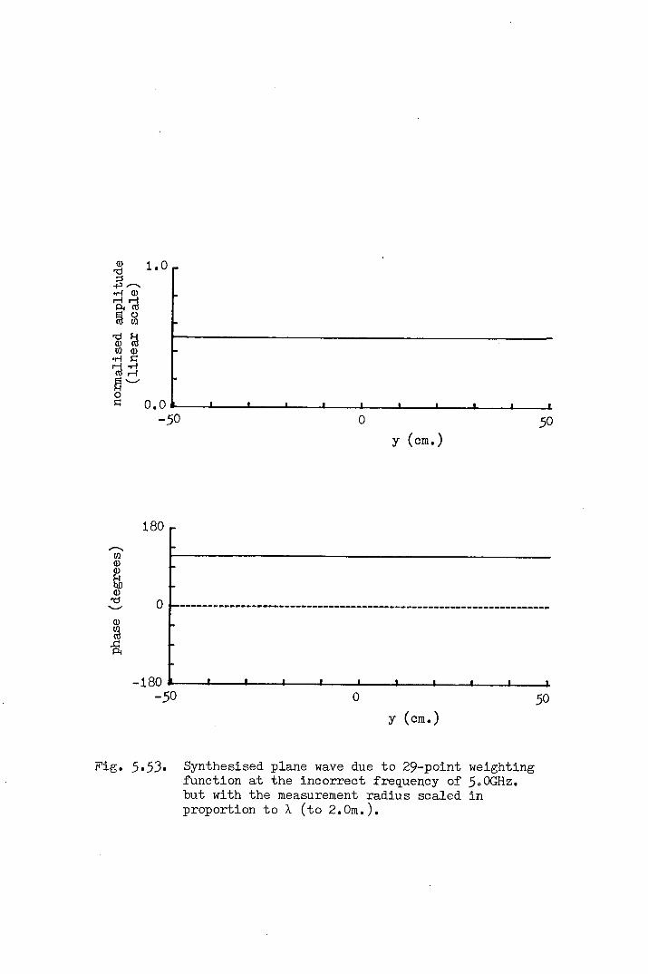
Q) 1.0'd~~..---..·rI Q)

~~@ s~ ~II.l Q)·rI 5:l

~~t:j'-'05:l 0.0

-50 0 50y (cm, )

180..---..II.lQ)Q)!-leoQ)'d 0'-'Q)

~..c:Pt

-180-50

-------------------------------------------------------------------

o 50y (cm.)

Fig. 5.53. Synthesised plane wave due to 29-point weightingfunction at the incorrect frequency of 5.0GHz.but with the measurement radius scaled inproportion to A (to 2.0m.).

-96-

6. THREE-DIMENSIONAL VERIFICATION

TO verify the technique in its full three-

dimensional configuration a 45cm reflector antenna was

evaluated at X-band and this chapter is concerned primarily

with describing the experiments and the results. Before

carrying out the experiments, however, it was necessary to

set up the measurement equipment in the anechoic chamber at

the University of Sheffield antenna test range and the

details of this are discussed first.

6.1 Antenna Test Range and Equipment

The Departmental antenna test range is located on a

fairly rugged site at Harpur Hill near Buxton in Derbyshire

about 30 miles from Sheffield. The site is quite elevated

and remote so that interference from terrestrial sources is

at a relatively low level. There are a number of possible

measurement ranges available, the longest of these being

across a valley to a distant hillside on which a transmitter

may be located at a distance of up to 3 miles from the

Departmental buildings, antenna tower, etc. Within the site,

various ranges are available (using hillside locations, etc.)

of up to about 150m and one of particular relevance gives a

measurement range of approximately 30m. This range stretches

between the roof of the main Departmental bunker and a metal

tower at a similar height (about 12ft above ground level)

built originally to support a fairly heavy duty Scientific

Atlanta '(S.A.) elevation over azimuth positioner system (not

used for these experiments). This was the range used for

the far-field measurements of the 45cm reflector.

-97-

The near-field measurements on the antenna were

performed in a small radio-anechoic chamber located inside

the main bunker (along with the control room). The chamber

is about 8m in length and is of square cross-section tapering

from about 2.5m square at the positioner end to about 60cm

square. The chamber is lined with Plessey absorbing materials

types AF20 to AF24 along the sides and type AF50 on the large

rear wall. A small azimuth turntable (S.A. type 5103) was

originally mounted on a pair of steel rails allowing 1m

longitudinal adjustment within the quiet zone.

For the present measurement programme various new

items of equipment were purchased and others designed and

built in-house. To obtain the complete spherical scan capabil-

ity another positioner was required to mount over the existing

azimuth turntable. To fulfil this requirement an S.A. type

56060 polarisation positioner was chosen. A rigid mounting

unit was then designed to hold the polarisation positioner

on the azimuth turntable. The design was complicated by the

90kg load limit on the azimuth turntable but a suitably rigid

construction was achieved. This may be seen in Fig. 6.1.

Related to the rigidity ~f the system, it was also

found that the existing support rails were too flexible and

these were replaced with a new structure of heavy duty steel

beams bolted to the floor and cemented in place.

On the probe side, a scalar feed had recently been

constructed within the Department, for use at 11.7GHz in

another project and it was decided that this would form a

suitable device with a smoothly varying and therefore easily

defined radiation pattern. In addition it possessed the

desirable attribute of circular symmetry. Behind the probe,

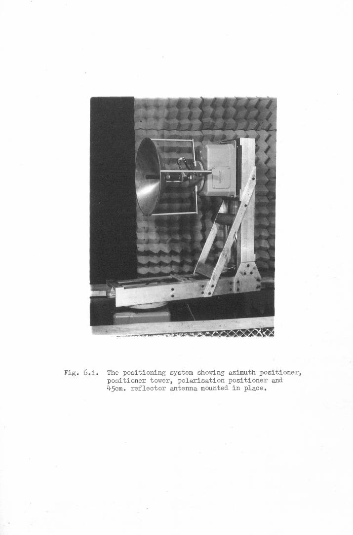
Fig. 6.1. The positioning system showing azimuth positioner,positioner tower, polarisation positioner and45cm. reflector antenna mounted in place.

-98-

some equipment for selecting one of two orthogonal probe

polarisations was required. For this purpose, an Andrew

Antennas model 64l00A-107 dual polarised circular to

rectangular waveguide transition was selected. This item

has a specified frequency bandwidth of lO.7GHz to 11.7GHz.

In order to switch between the two ports of the wave-

guide transition, an R.F. switch was necessary and the Hewlett

Packard 333llB coaxial switch was considered suitable with

bandwidth from D.C. to l8GHz, very high port-to-port isolation

(typically in excess of lOOdB at X-band) and with the

particularly useful property of internal termination of the

ungated R.F. port in son to avoid mismatch and consequent

reflection problems. The probe was selected to be the

transmitting antenna and the microwave source used was a Gunn

diode delivering approximately lOmW at a frequency of 11.7GHz.

Fig. 6.2 shows the probe with dual polarised transition behind

it and the microwave switch is just visible on the photograph.

A cable reference was taken to the receiver from the Gunn

diode via a directional coupler.

Careful setting and alignment of the mechanical subsystem

was, of course, a prerequisite to acquiring the data and this

will be outlined a little later. Next, however, is given a

brief description of the parts of the data acquisition and

control subsystems held within the control room of the test

facility.Basic control of the S.A. positioners was by means of

two model 4111 position controllers. These are essentially

manual control devices but some in-house modifications meant

that a remote drive on/off control function could be exercised

Fig. 6.2. The probe assembly before coating in absorber. The scalarfeed probe is on the right, the dual polarised waveguidetransition towards the left and the coaxial microwaveswitch is just visible on the extreme left.

-99-

from a purpose built remote control unit commanded by a

Ferran~i Argus 600 minicomputer, a very basic machine with

only 2k-bytes of memory and a very limited instruction set.

The position information was derived from an S.A.1842A

synchro-to-digital position indicator connected, again

under computer control, to the selected positioner (only

one positioner can be operated at anyone time).

In addition to scan control, the Argus minicomputer

controlled the data acquisition. The polarisation of the

data was selected by the computer via a locally designed

and built drive unit for the Hewlett Packard R.F. switch.

This unit incorporated the appropriate logic functions for

computer control together with the drive circuitry for the

switch and an electromechanical counter to keep a tally of

the total number of switching operations performed. For the

far-field measurements, this was later slightly modified to

incorporate a "drive boost" facility to enable the switch

to be driven through in excess of 100m of cable.

The receiver used was an S.A.17S4 two-channel phase

and amplitude receiver (one signal channel plus reference

channel) and the preliminary scans taken to verify the

operation of the R.F. and mechanical aspects of the system

were recorded on an S.A.lS23 (rectangular) chart recorder.

For the data scans themselves, the analogue signals from

the receiver were converted to digital form by an S.A.1833A

amplitude ratiometer and an S.A.1822A phasemeter (to aoresolution of O.ldB and 0.1 ) and output onto punched paper

tape by the Argus 600.

-100-

6.2 System Alignment

It is important that the system should be set-up

mechanically as accurately as possible to enable good quality

data to be obtained. This has various aspects:

(a) Probe position and pointing accuracy.

The probe should point accurately towards the origin

of the coordinate system (the centre of rotation). It should

be at the same height as the polarisation axis and the

distance from the probe to the centre of rotation should

be known.

(b) Orientation and intersection of positioner axes.

The axis of the azimuth turntable should be truly

vertical, the axis of the polarisation turntable should be

truly horizontal and the two axes should intersect accurately

in space.

(c) Positioner pointing accuracy.

The system should be set up so that, when the azimuth

positioner is set at 00, the axis of the polarisation positioner

should be pointing at the centre of the probe.

The effects of these mechanical errors have been

discussed to some extent in Chapter 5. Here, the methods

used to avoid the errors are detailed.

For the setting-up procedure, five main items of

equipment were used:

(1) A sensitive spirit level.

(2) A sharply pointed rod in a mounting device with a 4-screw

fine lateral adjustment mechanism. The mounting device should

have a base suitable for clamping onto the azimuth turntable

(or similar surface) so that it can point along the vertical

-101-

azimuth axis with the polarisation positioner mounting unit

in place. The length should be adjustable.

(3) Another sharply pointed rod in similar adjustable

mounting unit with mounting holes suitable, this time, for

the polarisation turntable to enable the rod to point along

the horizontal polarisation axis. Spacers should be provided

to hold the base approximately 2cm off the turntable. Anangled viewing hole (approximately lcm diameter) should be

drilled in the base plate for a purpose which will be

described below.

(4) A flat plate bearing a finely scribed cross at its.

centre with mounting holes suitable for the polarisation

turntable.

(5) A precision optical level with fairly high magnifica-

tion and crossed hair sights.

For the last item, a Sokkisha BI-C precision automatic

level with 32x magnification (see Fig. 6.3) was purchased.

Sensitive spirit levels were already available within the

Department and the other devices were manufactured in the

Departmental workshop.

6.2.1 The Alignment Procedure

The details of the procedure for setting-up the

mechanical alignment of the system (which should be already

assembled) are as follows:

(a) Enqure that the axis of the azimuth turntable is vertical.

This is achieved by placing the sensitive spirit level on the

turntable which is then set in motion. The mounting screws

on the turntable base are adjusted until the bubble in the

level remains stationary as the turntable rotates. It should

Fig. 6.). The optical level used for system alignment.

-102-

be emphasised that the bubble does not have to be centred in

the level (and in general will not be so) since the adjustment

for a vertical turntable axis does not imply that the turn-

table face is exactly horizontal.

(b) Set the scribed cross of the metal plate to be on the

axis of the polarisation positioner. The plate is mounted on.

the polarisation turntable which is then rotated. The centre

of the scribed cross is viewed through the optical level

(lined-up on the crossed hairs) and its position on the

turntable adjusted until the centre of the cross appears to

remain fixed in space as the turntable rotates.

(c) Set up the first of the pointed rods vertically so that

the tip is on the axis of the azimuth turntable. The pointer

is mounted approximately above the centre of the turntable

and its length is adjusted so that its point is as nearly as

possible level with (or fractionally below) the axis of the

polarisation positioner. The pointer is then laterally

adjusted until its tip appears fixed in space when viewed

through the optical level.

(d) Set the tip of the second pointer on the axis of the

polarisation positioner. The second pointer is mounted at

the centre of the polarisation turntable over the scribed

plate (using the spacers). The length is adjusted so that

the point is almost coincident with the azimuth axis pointer.

At this stage, it may be found that the length of the latter

was set too great or too little. If so, this may be corrected

but it will then be necessary to return to step (c) to check

its lateral setting. The polarisation positioner is then set

in motion (cautiously at first, lest the two points should

-103-

collide and damage one another - care should be taken for

this possibility in the following two steps also) and the

lateral position of the second pointer is adjusted in a

similar manner to step (c) so that the tip lies on the

polarisation axis. Fig. 6.4 illustrates this stage.

(e) Make the polarisation axis horizontal. This is the

point at which the viewing hole in the base plate of the

second pointer comes into play. The azimuth and polarisation

positioners are rotated into such positions that the cross

on the scribed plate is visible (careful lighting arrangements

may be necessary at this point) through the viewing hole.

The optical level is carefully adjusted to be at the same

height as the centre of the cross and then panned horizontally

to look at the polarisation axis pointer. The mounting screws

of the polarisation positioner are adjusted to bring the tip

of the pointer up to the same height. This adjustment may

have changed the height of the scribed cross so that the

procedure should be repeated several times until the tip of

the pointer and the cross are at the same height.

(f) Make the axes intersect in space. The azimuth turn-

table is rotated so that the polarisation axis pointer is

viewed end-on. The position of the polarisation positioner

is adjusted in the transverse direction until the tips of

the two pointers almost coincide. If the two pointers are

not close enough (or are so close that they are likely to

touch) the length of one or both of the pointers may have

to be adjusted in which case a return should be m~de to

step (c) or (d). depending on which pointer(s) has been

adjusted. Otherwise, when the transverse position of the

Fig. 6.4. The positioning system with alignment painters inplace.

-104-

polarisation positioner has been adjusted as precisely as

possible (the polarisation axis pointer should appear

vertically above the azimuth axis pOinter), the other

adjustments from step (e) should be re-checked and this

procedure should be repeated until no further adjustment

is required. If the distance between the pointer tips is

O.Smm, for example, and the vertical can be judged to anaccuracy of 50 (considerably better accuracy than this is

to be expected) then the error introduced by this will be

less than O.OSmm.

(g) Set up the probe height and horizontal. In many

probe mounting systems, it is likely that the central line

(in height) of the probe will be defined by the joining

lines of the clamps. If not then a datum line should be

marked out in advance. Whatever line is used, this should

be adjusted to be horizontal and at the same height as the

centre of rotation by the same panning technique as used

in step (e).(h) Set the probe azimuth. Again, the central line of the

probe in the longitudinal direction may be obvious or it may

be necessary to mark this out on the mounting bracket (front

and back). Using whichever method is convenient, the centre

of rotation is viewed from the end of the chamber and the

probe pointing adjusted in azimuth until looking along the

same line. If the probe azimuth adjustment mechanism cannot

be guaranteed to give an accurate azimuth sweep, it may be

necessary to return to step (g) to check the probe height

and horizontal.

-105-

(i) The azimuth pointing of the scanning system is

finely adjusted. The optical level is set up looking from

behind the probe (as left by step h) along its axis to the

centre of rotation. The polarisation axis pointer is

removed and the azimuth zero is set up at the point where

the centre of the scribed cross on the plate beneath lines

up with the probe.

(j) The probe is inserted in the mounting bracket and

its longitudinal position finely adjusted (it is assumed

that the coarse setting up of the distance will have been

done when the probe mounting system was originally positioned)

to give the required measurement distance.

(k) All alignment equipment is removed and the scan may

proceed.

It is anticipated that with the use of the technique

described and the equipment presently being employed, setting

accuracies of O.lmm or better can be achieved.

6.2.2 The Test Antenna

The antenna under test was a 45cm diameter aluminium

focal-plane reflector fed from what has been described as

a "splash-plate" feed(37) which is similar to but much simpler

than the feed described by Silver(38) and from the appearance

of the data, has a somewhat mediocre performance. The

antenna was mounted onto the polarisation turntable by four

aluminium arms holding the dish at the perimeter.

Additional support was supplied by the cable attached to

the rear. of the feed via the harmonic mixer. The test

antenna is shown set up ready for scanning in Fig. 6.5.

Fig. 6.5. The positioning system set up ready for a scan.

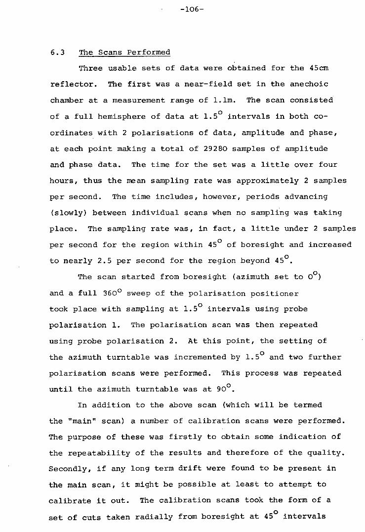
-106-

6.3 The Scans Performed

~hree usable sets of data were obtained for the 4Scm

reflector. The first was a near-field set in the anechoic

chamber at a measurement range of l.lm. The scan consisted

of a full hemisphere of data at 1.50 intervals in both co-

ordinates with 2 polarisations of data, amplitude and phase,

at each point making a total of 29280 samples of amplitude

and phase data. The time for the set was a little over four

hours, thus the mean sampling rate was approximately 2 samples

per second. The time includes, however, periods advancing

(slowly) between individual scans when no sampling was taking

place. The sampling rate was, in fact, a little under 2 samples

per second for the region within 450 of boresight and increased

to nearly 2.5 per second for the region beyond 45°.

The scan started from boresight (azimuth set to 00)

and a full 3600 sweep of the polarisation positioner

took place with sampling at 1.50 intervals using probe

polarisation 1. The polarisation scan was then repeated

using probe polarisation 2. At this point, the setting ofothe azimuth turntable was incremented by 1.5 and two further

polarisation scans were performed. This process was repeated

until the azimuth turntable was at 900.

In addition to the above scan (which will be termed

the "main" scan) a number of calibration scans were performed.

The purpose of these was firstly to obtain some indication of

the repeatability of the results and therefore of the quality.

Secondly, if any long term drift were found to be present in

the main scan, it might be possible at least to attempt to

calibrate it out. The calibration scans took the form of a

set of cuts taken radially from boresight at 45° intervals

-107-

of test antenna polarisation with both probe polarisations.

Since each of these cuts was taken over a short period of

time any slow drift occurring would show up minimally in the

calibration scan but if it were compared with the correspond-

ing cut extracted from the main scan, the slow drift present

there would appear as a varying discrepancy across the cut.

The second set of data was another near-field set

taken, this time, at a range of 1.5645m. The parameters of

the main scan and the accompanying calibration scans are

exactly as for the l.lm set.

For a comparison with the near-field predictions, the

remaining data were taken in the far-field on an outdoor 30m

range as described in section 6.1. In this case the outer

limit of the scans was 70.50 but otherwise the parameters

were the same thus indicating a total of 23040 sample points.

The equipment for these outdoor measurements was set up with

the probe (source) on the metal tower and the test antenna and

positioners (taken from the anechoic chamber) set up on the

bunker roof. This arrangement was chosen so that, as the

scan progressed away from boresight, the test antenna would

turn in azimuth to look away across a wide valley thus, it

was hoped, avoiding the worst of the ground reflection

problems. In addition, a wall of absorber was placed on the

ground between the probe and the test antenna at the

approximate specular reflection points.In'each case it was found to be of significant value

to take preliminary scans in the form of two boresight scans

of the polarisation positioner, one with each probe polarisation.

-108-

The results of these scans were logged on the chart

recorder for immediate examination. The expected pattern

in this case would be (a) cosinusuidal in form and (b)

identical for each probe polarisation apart from a 900

angular shift. Any significant variation in the first

case would be looked upon with suspicion (dependant upon

the nature of the antenna, for a paraboloidal reflector

the cosinusoidal form might be expected to be quite good)

while in the second instance any difference (apart from

constant amplitude and/or phase shifts) would certainly

indicate problems. Severe cable faults in both near and

far-field systems were revealed in this way and corrected.

Figs. 6.6 to 6.11 are examples of the measured data

showing H-plane co- and cross-polar cuts for each of the

data sets (comparing main and calibration scans in each

case). These are the raw data before any drift correction

or independent normalisation and display the effects of

quite severe drift, particularly in the case of the far-

field set. The sources of the drift are discussed at a

later stage but it is noted here that before using the

near-field data for predictions of the far-field, they were

corrected as far as possible for the amplitude and phase drift

present. It is interesting to note that in the case of the

l.lm data set, the amplitude and phase drifted equally

(about 0.9dB and 450) for both probe polarisations. In the

data set 'obtained at 1.5645m, on the other hand, while the

phase drift was similar (about 300) for both probe polarisa-

tions, only one polarisation exhibited any serious amplitude

drift (2dB). This point will also be covered later.

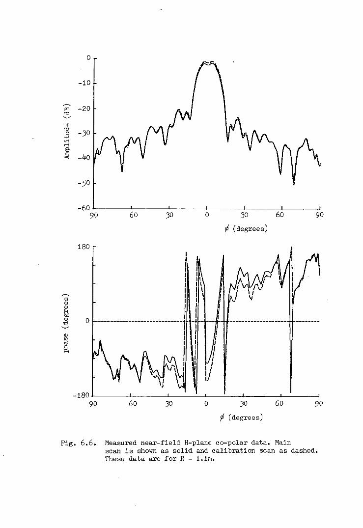
0

-10

........... -20~'--"

ID'd -30;::l+'.r!rlPo<s -40<

-50

-60~---------~---------~---------~---------~---------~------~90 60 30 o 30J6 (degrees)

60 90

180

o

IIIIIIJIIJIII----------------------------1JIIIIJIIfI

-180~---------+----------+----------+----------+----------+-------~90 60 30 o 30

J6 (degrees)60 90

Fig. 6.6. Measured near-field H-plane co-polar data. Mainscan is shown as solid and calibration scan as dashed.These data are for R = 1.1m.

o

-180~---------~---------~---------~---------~---------~~---~90 60 30 o 30

~ (degrees)60 90

Fig. 6.7. Measured near-field H-plane cross-polar data. Mainscan is shown as solid and calibration scan as dashed.These data are for R = 1.1m.

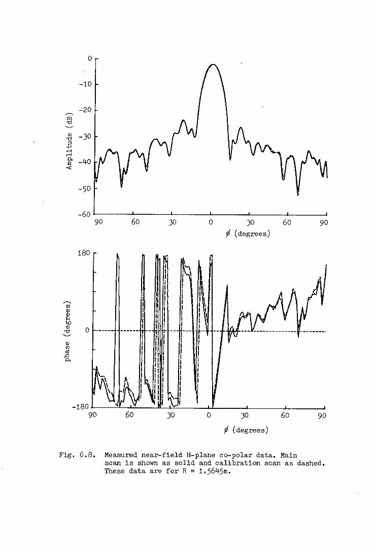
0

-10

-20,--...

~...___..ID -30'ti~+>·rir-!P. -40s<

"-50

-6090 60 30 0 30 60

~ (degrees)

180 .. r~I ~I I ,II II I II I I\

II I I I \,--...

~I I I \in IID I I \

ID II I I I \f.-I II I I IeoII I I I(J) 0'ti ----- ------ --- I--

'-' I I(J) I IUl I Iro I I.c I Ip. I II II II II II

~I

-18090 60 30 0 30 60

~ (degrees)

90

90

Fig. 6.8. Measured near-field H-plane co-polar data. Mainscan is shown as solid and calibration scan as dashed.These data are for R = 1.5645m.

o

-10

"""""_-20~

-50

-6090 30

180

I;--...

enIDIDf.ltillID 0'ti'--" IIID IIen IIro ".cPi II

1/II,

-18090 60

II

--------1 IItf;-II III ,II JI JI

IJ

I IJII '1

o 30f6 (degrees)

60

AIIIIIIIIII,,,,,lAI,I,II,,

30 90o 30pS (degrees)

60

Fig. 6.9. Measured near-field H-plane cross-polar data. Mainscan is shown as solid and calibration scan as dashed.These data are for R = 1.5645m.

r,0 I \

I \I ,I \I \

-10 I ,I ,I ,I ,, ,

r--. -20 ' ,~

I ,,.. I "\'--' 1'-' \ I " .....,ID \ '"'C -30 .....,' " \ I::s " \1~•.-1r-iPi /

"" -40<

-50

-6060 30 0 30 60

~ (degrees)

180

r--.UlIDIDf..I 0eoID'C'--'

IDUlcO.cPi

60 30 o 30~ (degrees)

Fig. 6.10. Measured far-field H-plane co-polar data. Main scanis shown as solid and calibration scan as dashed.The apparently unusual shape of the calibration scanmain beam is because, due to the severe drift, thetwo halves of the calibration scan (taken separately)did not meet at boresight.

o

-10

,-.._ -20~'-"

Q)'"d -30~-r>'M.--i

~ -40<

-50

-6060 30 0 30 60

180 ~ (degrees)ItJI

11 I,-.._ IUl IQ)Q) IIf..l ,Itu> , IQ)'"d 0 ' I'-"

Q)Ulro.cPi

, IIVI

60 30 o 30~ (degrees)

60

Fig. 6.11. Measured far-field H-plane cross-polar data. Mainscan is shown as solid and calibration scan as dashed.

-109-

6.4 Far-field Predictions

Earlier chapters (in particular Chapter 3) have

included details of the creation of a primary weighting

function including the iterative optimisation and the

method of converting it into a composite weighting function

possibly for a different geometry (Chapter 4). The first

of these two operations requires a fairly powerful computer

and so, to date, one of the CDC 7600 machines at the

University of Manchester Regional Computing Centre has been

used. For the antenna size under test here, it has been

found that a CPU time of typically 4 minutes has been

required to achieve a primary weighting function. These

data are then transferred via a data-link to Sheffield for

use locally.

Prototype far-field prediction software was written

for the main University ICL 1906S computer and an earlier

set of data (not described in this thesis) was processed

by this means. This early version did not create a

separate composite weighting function but interpolated the

measured data directly.

The more recently developed software has been used

on the Departmental Varian (now Sperry Univac) V-72 image

processing computer. This machine is described in detail

in Appendix 4. The software developed, to date, for

processing the data is described in Appendix 5.

The first set of data to be processed was that

obtained with the 1.lm measurement range. The E-p1ane

co-polar and H-p1ane cross-polar patterns were predicted.

Because of the differences between the measured E-plane

-110-

co-polar main and calibration scans (the normalised curves

of E-plane co-polar measured far-field patterns are shown

as Fig. 6.12) it has proved useful to compare the prediction

with both of these and so Figs. 6.13 and 6.14 compare the

predicted E-plane co-polar pattern with the measured main

scan data and the calibration scan data. In the former,

a slow drift of quite severe proportions is observed in

the area well away from boresight.

The H-plane cross-polar main and calibration measured

patterns (Fig. 6.15) display significant differences in

places particularly in the region between boresight and 150.

In Figs. 6.16 and 6.17, the prediction from l.lm data of

this pattern cut is compared again with the measured and

calibration scans. It will be noticed that there are

quite substantial discrepancies but in general the

predicted cross-polar pattern is at a lower level than the

measured. The possible reasons for this will be discussed

later in the chapter. Some similarity in the broad side-

lobe structure is discernible.

Moving on to the predictions from the 1.S6m data,

Figs. 6.18 and 6.19 display comparisons between the

prediction of the E-plane co..Jpolarpattern and the measured

main and calibration scan data. It seems that within the

area less severely affected by the drift encountered during

the far-field measurements, the comparison between the

prediction and the meas .-ed main scan data is the superior.

Again, some likely reaS(lns for this will be discussed in

the next section.

-20,.-...

~<:»

ID -JOrrj;::l+l.r!rl

! -40

v-50 ,

o

-10

JO-60~------~~------~--------~------~

60 o JOrJ (degrees)

60

Fig. 6.12. Normalised measured far-field E-plane co-polaramplitude pattern. Main scan is shown as solidand calibration scan as dashed.

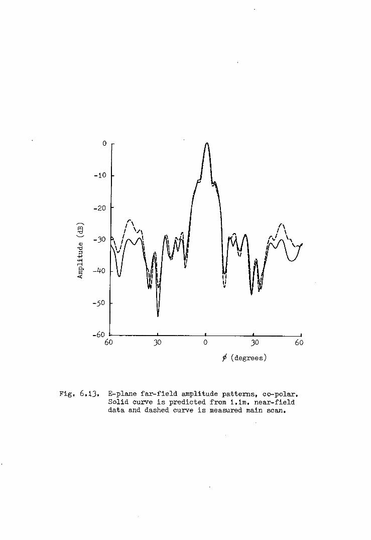
o

-20,.-...

~'--' -30Q)'d:::l~.r-!rl

~ -40-<

-10

-50

30 o 30~ (degrees)

60

Fig. 6.13. E-plane far-field amplitude patterns, co-polar.Solid curve is predicted from 1.lm. near-fielddata and dashed curve is measured main scan.

-20r--..

~...__.Q)re -30::;l~.r!r-iP;

~ -40

o

-10

-50 v,

-60~------~--------L-------~------~60 30 0 30 60

~ (degrees)

Fig. 6.14. E-plane far-field amplitude patterns, co-polar.Solid curve is predicted from 1.lm. near-fielddata and dashed curve is measured calibration scan.

o

-10

-20;--..

~ '\'-" \ID -30 \'t1 \;:$ \+'.r! \r-I \~ \-< -40 I,,,

II

-50 IIII

tI-6060 30 0 30 60

f6 (degrees)

Fig. 6.15. Normalised measured far-field H-plane cross-polaramplitude pattern. Main scan is shown as solidand calibration scan as dashed.

o

-10

-20,..--.,.

~'--"

Q)'T:1 -JO::1~•.-1.-f

~ -40rJ\( \ 1\ ~J \ I \ " ..I,J \ I \ '\ I \ I

-50 J \I ""VJ \ I , JJ ,I

-6060 0 JO 60

~ (degrees)

Fig. 6.16. H-plane far-field amplitude patterns, cross-polar.Solid curve is predicted from 1.1m. near-fielddata and dashed curve is measured main scan.

o

-10

-20r.....

~'---"

ID -30'd

E \.r-!rl l' \~ I' I \-< -40 I I

, ~I I , .../ \

'\ I I I II J I I II \ JI I

-50 I IJJ

-6060 30 0 30 60

f; (degrees)

Fig. 6.17. H-plane far-field amplitude patterns, cross-polar.Solid curve is predicted from 1.1m. near-fielddata and dashed curve is measured calibration scan.

o

-10

-20_.--"

~'-'"

ID -JO"Cl;::!.p.r!,...;

~ ,< -40 d I,

I II ,'I

-50

-6060 JO o JO

f6 (degrees)

60

Fig. 6.18. E-plane far-field amplitude patterns, co-polar.Solid curve is predicted from 1.5645m. near-fielddata and dashed curve is measured main scan.

-20".......

!::3'-"

ID -30'd

E• ..-lrl

~< -40(

"-50 v,

o

-10

30-60 -----------~~----------.------------~---------~

60 o 30rf (degrees)

60

Fig. 6.19.' E-plane far-field amplitude patterns, co-polar.Solid curve is predicted from 1.5645m. near-fielddata and dashed curve is measured calibration scan.

-111-

The remaining prediction presented here is the

H-plane cross-polar pattern predicted from the 1.56m data

(Figs. 6.20 and 6.21). In general, the agreement with

the measured far-field is better in this case than in the

prediction from l.lm data. It is rather difficult to make

a decision as to which of the two measured far-fields (main

or calibration scan) agrees best with the prediction exceptofor the region 0 < ¢ < 15 where the comparison with the

calibration scan is clearly the better.

Before embarking upon a discussion of the possible

sources of errors two more comparisons might prove to be of

value. These are between the predictions of the E-plane

co-polar (Fig. 6.22) and H-plane cross-polar (Fig. 6.23)

patterns obtained from the two different sets of near-field

data. Apart from some level shifts, the overall agreement

in the main pattern shape for both cuts is very encouraging.

6.5 Pattern Discrepancies

The sources of discrepancies between the far-field

predicted and measured patterns may be assigned to three

broad areas; (a) errors in the measured near-field data,

(b) errors in the measured far-field, (c) errors introduced

by the processing. Some of the possible sources of errors

observed in the data for the 45 reflector are investigated

below as they fall into these areas. The reader is also

referred to Chapter 5 where the topic of processing errors

is covered more generally (rather than specifically as

applied in the present measurements) .

In the measured near-field data, some element of

frequency drift is believed to be present. Although the

-20,,-...

~'-../

Q)"J:j -30;:::!+>.r!rl

~ex: -40

o

-10

-50

-6060 60o 30

" (degrees)

Fig. 6.20. H-plane far-field amplitude patterns, cre66~polar.Solid curve is predicted from 1.5645m. near-fielddata and dashed curve is measured main scan.

o

-10

-20,....,_~'-"

ID'"tj -30;::l+''Mr-i l'~ ,< -40

-50

-6060 30 o 6030

f6 (degrees)

Fig. 6.21. H-plane far-field amplitude patterns, cross-polar.Solid curve is predicted from 1.5645m. near-fielddata and dashed curve is measured calibration scan.

-20r--.

~<;:»

ID -30'ti.a.r!r-I

~-< -40

o

-10

-50

-60 L- ~ ~ ~ ~

60 30 o 30 60

r} (degrees)

Fig. 6.22. Predicted E-plane co-polar amplitude patterns.Solid curve shows prediction from 1.1m. near-fielddata and dashed shows prediction from 1.5645m.near-field data.

-20,......._

~'--"

Q)'t:I -30.B.,-jr-I

i -40

o

-10

-50

-60 L-~-u~~~~~--~----~--LL------~~60 30 0 30 60

Ji (degrees)

Fig. 6.23. Predicted H-plane cross-polar amplitude patterns.Solid curve shows prediction ,from 1.1m. near-fielddata and dashed shows prediction from 1.5645m.near-field data.

-112-

usual efforts were made to equalise the electrical path

Lerrqtihsof the signal and reference channels, there was

almost certainly a difference between the two. In the

presence of a drift in the measurement frequency, such a

path length difference is manifested as a phase drift.

The measurement frequency was nominally 11.7GHz but it

is now believed that the Gunn diode source used was

probably not sufficiently stable to provide really

accurate results. In the first set of near-field data,

a drift of up to 450 in phase was observed. If the

approximate formula,~ljJ = 2TIN~f

f. (6 • 1)

is applied, where f = test frequency, ~f = frequency change,

N = electrical path difference in wavelengths and ~ljJ =relative phase change, and a possible path length difference

of 30A is assumed, this would indicate the serious frequency

drift of 48MHz. This is based, of course, on the assumption

that all of the phase drift is due to the combination of

frequency drift and electrical path difference. This will

not, in fact, be the case. In the practical system there

will be other sources of drift. The attenuation of cables

will vary with frequency as may the characteristics of the

harmonic mixers used. A likely cause of drift will be

temperature variation and this leads us to consider other

factors not directly related to frequency. The behaviour

of hardware items such as the directional coupler may vary

with temperature but probably much more significant will be

temperature sensitivity of the mixers. One other significant

point may be expansion effects on the mechanical parts causing

-113-

the alignment of the system to yary although tests have

indicated that this is probably not occurring to a large

extent here.

The phase drift in the second set of near-field data

was rather less (approximately 300) but in this set, another

effect becomes apparent: differe~tial amplitude drift between

the two probe polarisation channels. It is suspected that

a possible cause of this is that the frequency drifted above

11.7GHz which is the specified upper limit for operation of

the dual polarised waveguide transition. The first (unaffected)

port of the device is coupled directly into the circular wave-

guide but the second port (the one exhibiting the drift) is

via a pin-twist in the circular waveguide and this is likely

to be the frequency sensitive component.

Apart from the possible distortion of the hardware

with temperature, it is believed that using the setting-up

techniques described, errors associated with system static

misalignment are not significant. The other source of

positioning errors will be the fact that the equipment is

in motion during the sample. The sample command is issued

by the control computer at the moment that the specified

angle is reached but there is a finite integration time

involved wit~ obtaining the sample which means that there

will be a smearing effect over the area from the required

sample position to some position beyond this,dependent

upon the 'integration period and the scan speed. At theoscan speed of 3 per second and with an integration time

of 10 ms (the value used) the smearing effect will extend

over 0.030. At a region of constant field, this will

-114-

introduce no error while if there is a linear amplitude

gradieRt equivalent to 20dB per degree the effective

amplitude error will be of the order of O.ldB. It is

to be expected that amplitude gradients exceeding this

value will be fairly rare so that it is felt that a scan

speed of 2 samples per second with 1.50 sampling interval

will be satisfactory. In spite of this, it is noticeable

that, in both near-field scans, there is a slight increase

in the discrepancies between main scan and calibration scan

data in the region beyond 450 from boresight where the

speed of scanning was increased slightly. This will also

be associated, however, with the fact that this region is

one of lower sidelobes where the signal to noise ratio might

be expected to be worse. Since the apparent speed-dependent

errors seem to be of a magnitude no greater than the inherent

noise, they are probably of no greater significance. It is

recognised that it would not be desirable to increase the

speed much beyond the level of 2.5 samples per second.

Chamber reflections may be of some significance, but

it is anticipated that since the experiments were set up in

the best part of the chamber, the effects are probably quite

small.

As mentioned previously, the far-field measurement set

up too was designed to minimise range reflections but

inevitably, these will be present to some extent. Any

effects of these will, however, be totally masked by the

much more significant error introduced by the severe

temperature drift. The far-field measurements extended into

the early hours of the morning by which time the temperature

-115-

had dropped markedly. Over a period of about 30 minutes,

it was'possible to observe the amplitude of the reference

channel fall by over 10dB due to a combination of falling

source level and almost certainly extreme temperature drift

in the mixers. The effects are quite apparent in the graphs

of raw far-field data (Figs. 6.10 and 6.11).

One other measurement error is particularly relevant

to the predictions of the cross-polar pattern. Because

of the height to which the probe had to be raised to bring

it level with the test antenna, it became very difficult to

set up the polarisation with any degree of confidence. The

measured cross-polar level is particularly sensitive to

polarisation error (e.g. at boresight, a polarisation

setting error of 30 means that the measured pattern will

be effectively the cross-polar level added to the co-polar

level attenuated by 25dB) so that the discrepancies between

the H-plane cross-polar predicted and measured far-field

patterns could well be attributable in a large part to

polarisation error setting. It should also be recognised

that the pattern along the cross-polar null is likely to

be relatively sensitive to frequency difference. Indeed,

the measured near-field is also likely to be affected

comparatively severely by the frequency changes.

The quality of the synthesised plane waves for the

l.lm and 1.56m weighting functions are illustrated with a

single co-polar cut of each in Figs. 6.24 and 6.25. It is

clear that the quality of the latter is better and this is

largely attributable to the fact that the former was

allowed to undergo only seven cycles of the iterative

1.0

Q)

"~.~a.. 0.5E"'s..."'Q)c

0.0-24 -12 0 12 24

y (Gm)

Fig. 6.24. Central cut of synthesised plane wave, co-polar,due to weighting function at 1.lm.

Q)

"~......,o, 0.5E"'s...esQ)C

0.0-24 -12 0 12 24

y (cm)

Fig. 6.25. Central cut of synthesised plane wave, co-polar,due to weighting function at 1.5645m.

-116-

process whereas the latter was allowed twelve. Treating

the ripple in the l.lm synthesised plane wave in the manner

described in Chapter 5 would suggest a spurious far-field

source at approximately 16.50 from the desired source with

the harmonics of the ripple appearing as sources at 350oand at 58. It is interesting to note that some of the

worst discrepancies between the measured and predicted

patterns occur at these angles. For the 1.56m plane wave,

the ripple is generally at a rather lower level and indeed

the far-field discrepancies at the above angles also seem

overall to be rather less.

Particularly interesting as regards two other possible

error sources is Fig. 6.22 which compares the two predictions

of the E-plane co-polar pattern. In the region outside the

main beam, the shapes of the two predictions are very similar

but the prediction from the l.lm data is at a consistently

lower level than that from the 1.56m data. There are various

possible sources for such an error for which one candidate

must be the slow drift which took place. In view, however,

of the attempt at calibrating out the drift it was felt that

the residual drift effects would probably not be manifested

in this fashion. Another possible source which was considered

was a slight misalignment between azimuth zero and the

position of the probe. This would result in one prediction

of the pattern passing near the peak of the main beam while

the othe~ might miss the beam peak slightly. Under normal-

isation, this would appear as a shift of the sidelobe level.

This argument may be rejected as defining a serious con-

tributor to the errors when the figures are calculated which

-117-

indicate that, at the very least, the probe would have

to be displaced by several millimeters to produce the sort

of effects present.

Another examination of the synthesised plane waves

(Figs. 6.24 and 6.25) gives us a clue as to what might

produce this sort of effect. The ~emaining major feature

not already mentioned is the presence of a small peak (in the

1.56m case) or a small dip (in the l.lm case) at the centre

of the synthesised plane wave. By the same sort of arguments

as applied to the ripple components, it can be seen that a

delta function at the centre of the synthesised plane wave

will appear not as a spurious far-field source at a

particular angle but a substantially constant "background

level" at all angles. In the area of the main beam, with

normalisation having been carried out, this effect will not

be noticeable but in the sidelobes it may well become of

significance. One remaining point which could have a bearing

on this discrepancy is that the probe has not been fully

characterised, as yet, and therefore the approximation of

a half-wave dipole field pattern has been used for the

probe compensation. It may be that this approximation is

not sufficiently accurate. Clearly any error in this

respect will be more serious at the wider angles of the

probe which in turn means that it will appear more serious

in the l.lm near-field data.

In conclusion of this chapter it may be said that the

far-field predictions are encouraging but display certain

errors for which a large.number of possible sources have been

suggested. Some of the future work in th~ development of

-118-

plane wave synthesis will be directed towards investigation

of which of the error sources are important and how they can

be reduced.

-119-

7. CONCLUSION

7.1 Summary of the Work to Date

A technique has been elaborated which it is

believed will be capable ultimately of providing predictions

of far-field antenna radiation patterns from near-field

measurements with an accuracy at least comparable with exist-

ing transformation schemes. Furthermore, most of the onerous

part of the processing is in fact performed in advance so that

this need only be carried out once for a particular antenna

size at a particular frequency and the precalculated

coefficients held in the form of a library of weighting

functions each of which might have an approximate 10% band-

width as shown in Chapter 5. The actual prediction process

contains only complex number multiplications and additions

which makes it relatively simple to implement.

In Chapter 2, the processes of the formation of a

synthesised plane wave from a weighting function were

examined and the various effects leading to imperfections

were discussed. Particularly enlightening were the displays,

in grey scale, of the field distributions over an area,

where it could be seen that some of the worst problems in

formation of a high quality plane wave were due to inter-

ference between the main plane wave and the grating lobes

produced because of the spacing between weighting function

samples. Also in Chapter 2, the sampling criterion was care-

fully examined and a curve describing the necessary reduction

in sampling interval with reduction in measurement range was

presented.

-120-

Chapter 3 considered the problems of the three-

dimensional sampling geometry, in particular the

elevation-over-azimuth system, and the necessary formulae

for production of a primary weighting function and its

conversion into a set of composite weighting functions

were given. In addition, because the sampling geometry

meant that interpolation was required in the transformation

from a primary weighting function to its composite equiva-

lents, a number of fairly simple interpolation schemes (all

four-point) were considered and it was concluded that the

four-point Everett interpolation scheme came out as favoured

by a small margin over the four-point Lagrange scheme, with

Fourier interpolation rejected because of its time consuming

function calculations and failure to reduce to the zero-

error condition for small sample intervals.

The equivalent formulae for the polarisation-over-

azimuth sampling geometry were presented in Chapter 4 and

in addition, because of the advantages to be gained in

terms of computer time, the necessary formulae for producing

polarisation-over-azimuth composite weighting functions from

elevation-over-azimuth primary weighting functions were

included.

An analysis of some of the types of practical measure-

ment errors which might occur, together with the possible

effects of such errors was included in Chapter 5. In

addition 'to the consideration of practical measurement

errors, some thought was given to certain types of

systematic errors. The problem of probe compensation was

studied and it was demonstrated that certain types of errors

-121-

were introduced by incorrect compensation, notably

changing of sidelobe levels and null positions. It was

demonstrated that compensation for even quite narrow

beam probes could produce distinct improvements in the

prediction. The technique of Fourier analysis of the

~ynthesised plane wave and non-ideal residual was introduced

as a means of quantifying the imperfections in a synthesised

plane wave and it was thereby shown that many of the worst

effects are due to the edge discontinuity of the weighting

function. It was demonstrated that the iteration procedure

reduces the edge effects quite effectively. Lastly the

frequency tolerance of a typical weighting function was

studied and it was shown that about a 10% bandwidth should

produce results at least as good as measurements at 2D2/A.Furthermore, by scaling of linear dimensions in proportion

to the wavelength, this bandwidth could be significantly

extended.

Chapter 6 detailed a practical measurement including

preliminary predictions and a discussion of the apparent

errors present and their sources. It was demonstrated that

the full three-dimensional prediction is feasible and can

produce useful results and with improved experimental

procedures and more stable equipment, substantial accuracy

improvements should prove possible.

7.2 Application to Other Measurement Systems

As indicated in Chapter 1, one of the aims of the

project was a technique applicable to spherical measure-

ments but also, ideally, adaptable to planar and cylindrical

measurements. It is felt that the plane wave synthesis

-122-

technique is indeed adaptable to these geometries, however,

it would need some modification. While in the spherical

geometry, the direction of propagation of the synthesised

plane wave is determined simply by the positioning of the

weighting function on the data sphere, in the cylindrical

geometry, this control can only be exercised in this way

for one of the scan coordinates and in the planar geometry,

not at all. It is thus necessary to develop a method of

producing weighting functions which synthesise plane waves

travelling at oblique angles away from them. An investiga-

tion has been performed (although still using a spherical

surface) of synthesising a plane wave travelling at an

oblique angle (although only a relatively small angle) and

was shown to be successful. The inherent separable variable

nature of these two other geometries may provide considerable

simplification in the generation of the weighting functions.

An offshoot of the plane wave synthesis technique

(which has developed into a separate project) uses a plane

wave synthesised by a single circular scan of a slotted

waveguide array. The illumination function of the array

provides one dimension of the weighting function and the

other is applied computationally, again utilising the

separable variable nature of the effective cylindrical scan.

Here, however, the test antenna is still scanned in a

spherical way producing a set of effective cylindrical

scans, the predictions being produced by computational

weighting of sets of one dimensional cuts of data. This(39) .has already been shown to produce useful results and

although theoretically not as flexible as the full plane

-123-

wave synthesis technique, could prove quite powerful in

certain circumstances.

7.3 Type of Probe

To date, a scalar feed has been used as the probe

because of its smoothly varying pattern with very low side

and back lobes, thus easy to characterise and not severely

prone to reflection from the support structure. This is

attached to a circular waveguide, the resulting system

being circularly symmetric. This circular symmetry is an

important property since the technique, as formulated in

this thesis, depends on the property for the ability to

obtain the desired probe polarisation by resolution of two

measured components. It would introduce further (although

not insurmountable) complications, if circular symmetry

were not able to be utilised since separate primary

weighting functions would need to be created with a knowledge

of the actual probe polarisations in each case.

Assuming the circular symmetry, it is clearly

desirable to have a probe with an easily definable pattern

but beyond this, any probe (assuming it does not have a

zero within th~ solid angle subtended by the test antenna)

is applicable as long as it is compensated correctly.

7.4 Processing Efficiency

To date, the software for producing the weighting

functions has been developed to perform its processing

efficiently (using the present approach) but the actual

prediction software has not been completely optimised. It

is feasible that the processing could be modified so as to

use the FFT to achieve the convolution of data with composite

-124-

weighting function in one of the dimensions and, if this

were implemented, calculations indicate that the prediction

of- the full far-field of the 4Scm reflector antenna might

be achieved in under 30 seconds of CPU time on the V-72

minicomputer presently being used for the processing. The

most time consuming part of the processing would then be

the initial generation of the weighting function and

certain ideas for improving the efficiency of this

process are currently being considered. Some of the more

promising ideas will now be mentioned briefly.

7.5 Efficient Weighting Function Generation

7.5.1 Small Antennas

The geometry which has been considered throughout

this thesis, for production of a weighting function by the

iterative procedure, has been with the weighting function

on a spherical surface and the plane wave on a planar

surface passing through or near the origin of the

coordinate system. This seems to provide the potential,

within the present computational limits, of providing a

weighting function to synthesise a plane wave 60A - aOA

wide. To be able to handle antennas larger than this, it

would be useful to be able to employ a modified geometry

which would make use of circular symmetry or some other

form of coefficient duplication to ease the processing

burden as regards the generation of the weighting function.

Since the weighting function is defined on a

spherical surface in an elevation-over-azimuth arrangement

of points, a logical way to define the synthesised plane

wave, so as to be able to exploit coefficient duplication,

-125-

would seem to be on a smaller concentric spherical

surface just outside the desired plane wave region, in a

similar elevation-over-azimuth geometry. This would mean

that the geometrical and probe pattern coefficients would

need only to be calculated for one elevation angle and

would apply equally for any other. This geometry will be

investigated as the plane wave synthesis technique is

further developed. Preliminary calculations suggest that

this may extend the maximum allowable antenna size to one

of the order of 200A.

7.5.2 Large Antennas

Ideas have been put forward that even larger antennas

might be manageable if optical-type approximations can be

made to suggest that a weighting function can be achieved

with little or no iteration by merely projecting the plane

wave back onto the spherical surface in phase (and resolving

into the appropriate field components), without any complicated

diffraction integral procedures. While such an idea is at a

very early stage of development, it may ultimately prove of

considerable value.

7.6 The "Standard" weighting Function

It was demonstrated in Chapter 5 that the frequency

range of a given weighting function could be extended by

scaling all the linear dimensions of the system in proportion

to the w~velength. In fact, theoretically, the bandwidth of

the weighting function could be made effectively infinite.

This leads to the proposition that a single weighting

function might be designed to produce a large, high-quality

plane wave and that by using the scaling technique, this

-126-

could be utilised to evaluate any test antenna (up to the

maximum allowable size) at any frequency.

This would unfortunately lead to overheads in terms

of an unnecesssarily large measurement range and unnecessarily

small sample interval for small antennas. It would, however,

be feasible to hold a small library of standard weighting

functions categorised according to electrical size of antenna.

The library might, for instance, consist of five weighting

functions covering the range up to l60A as follows,

weighting function 1 under lOAweighting function 2 lOA - 20Aweighting function 3 20A - 40Aweighting function 4 40A - 80Aweighting function 5 80A - l60A

If such intervals were considered too wide them more functions

could be held in the library as considered appropriate.

7.7 Conclusions

While much developmental work remains to be done to

convert the plane wave synthesis technique into a really

practical and reliable technique for performing an antenna

near-field/far-field transformation, it is believed that it

may eventually take its place as a valuable addition to the

range of near-field test techniques available. With improve-

ments along the lines of those suggested in sections 7.4 and

7.5, and with the continuing advances being made in computer

technology, particularly in the field of array processors,

the technique may have the capability of evaluating antennas

which at the present time can only be managed by the use of

severe paraxial approximations.

-127-

Appendix 1: IMPULSE RESPONSE OF THE WEIGHTING FUNCTION

.In section 2.2.2, it was shown in an analysis of

the basic processes taking place in the synthesis of a

plane wave that the actual synthesised plane wave

(neglecting the effect of the iterative procedure) is in

the form of the ideal plane wave convolved with an impulse

response approximating to a sinc (sin y/y) function. The

exact shape of the impulse response depends on, of course,

its position and also the weighting function geometry. In

this appendix, we study the impulse response at the centre

and at the edge of the plane wave region for various sizes

of weighting function.

All the diagrams shown here are for a weighting

function at a 1.Om measurement range and element spacingoof 2.0. In each case the response is illustrated on

three planes, z = 0 (the plane on which the impulse was

specified as input data), z = -lOcm and z = +lOcm. The

usual one-dimensional weighting function approximation is

used here.

Fig. Al.l shows the impulse response of a weighting

function covering the full semicircle (±90o) and, as

expected, the response on the plane z = 0 is quite narrow

but breaks down badly for z = ±lOcm. The analysis of

section 2.2.2 suggests that as the weighting function is

reduced in size, the impulse response will widen on the

plane z ~ 0 and will retain its properties better in

depth. As the sequence of figures shows, this conclusion

is borne out. The sequence is:

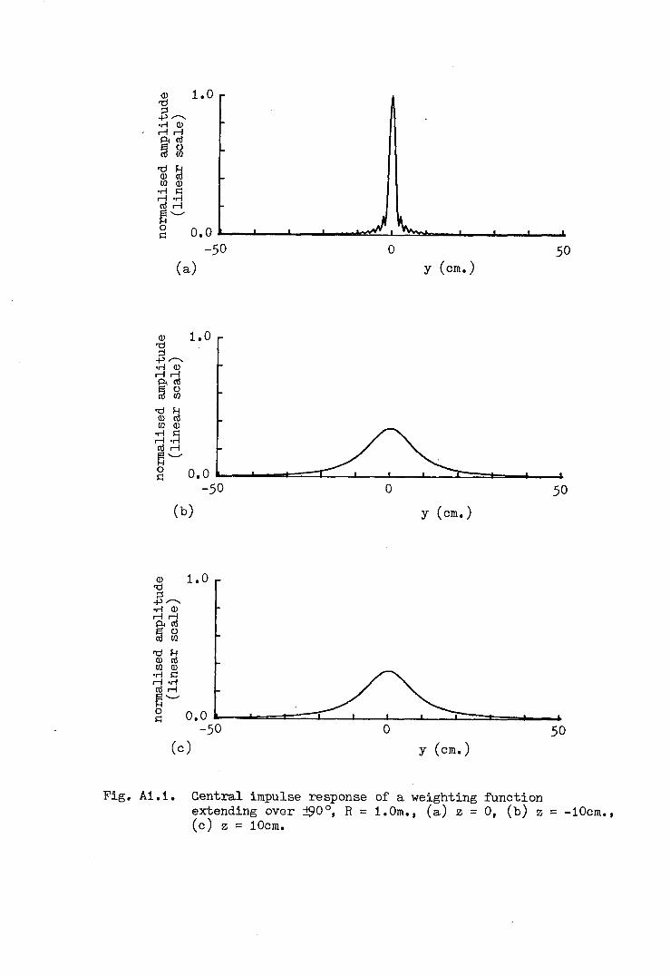
(a) y (cm.)

(b) y (cn; )

Cc) y (cm.)

Fig. Ai.i. Central impulse response of a weighting functionextending over 190°, R = 1.0m., (a) z = 0, (b) z = -iOem.,Cc) z = iOem.

-128-

Fig. A1.2 - ±60o weighting function.

.Fig. Al.3 - ±30o weighting function.

Fig. Al.4 - ±24° weighting function (by this timethe impulse response is maintainingitself much better in depth).

Fig. Al.S - ±20o weighting function.

Fig. Al.6 - ±16° weighting function.

Fig. Al.7 - ±12° weighting function (by which timethe impulse response is showing verylittle change over the 20cm depthdisplayed) .

In addition, a sequence of graphs is presented for

the same set of parameters as above but with the input

impulse offset lScm from the origin. This sequence is

as follows:

Fig. A1.8 - ±90o weighting function.

Fig. Al.9 - ±60o weighting function.

Fig.Al.lO - ±30o weighting function.

Fig.Al.ll - ±24° weighting function.

Fig.Al.12 - ±20o weighting function.

Fig.Al.13 - ±16° weighting function.

Fig.Al.14 - ±12° weighting function.

Again, it will be seen from these graphs that for

the wide weighting functions, the impulse response is

narrow but does not maintain itself well over any

appreciable depth while as the weighting function narrows,

the impulse response broadens but retains its properties

over a greater depth. It was also concluded in section

2.2.2 that the impulse response would undergo a scale

change with changing depth such that it would broaden

(a) y (cmo)

50y (cm.)

(c) y (cm; )

Fig. Ai.2. Central impulse response of a weighting functionextending over 160°, R = i.Om., (a) z = 0, (b) z = -iOcm.,(c) z = iOcm.

ID 1.0rO::s-j-l------.r! IDr-ir-i'Ptro@ g'g ~fI.l ID.r! s::::r-i .r!ror-l~--0s:::: 0.0

-50 0 50(a) y (cm.)

ID 1.0rO::s-j-l------.r! IDr-ir-iPtro@ g'2 ~fI.l ID.r! s::::r-i .r!ror-l~--0s:::: 0.0-50 50

(b) y (cm. )

(c)

Fig. A1.J.

y (cm.)

Central impulse response of a weighting functionextending over iJOo, R = 1.0m., (a) z = 0, (b) z = -10cm.,(c) z = 10cm.

<l> 1.0't:1::s+> r--...r! <l>MMP<cO@ s't:1 ~<l> cOt:I.l <l>.r! !::r-! .r!cOM~~0 0.0!::

-50 0 50(a) y (cm.)·

<l> 1.0't:1::s+> r--...r! <l>

11~@ g't:1 ~<l> cOt:I.l <l>.r! !::M .r!cOr-!~~0 0.0!::

-50 0 50(b) y (cm.)

<l> 1.0't:1::s+> r--...r! <l>r-!r-!P<cO@ gre ~<l> cOt:I.l <l>.r! !::r-! .r!cOr-!~~0 0.0!::

-50 0 50(c) y (cm.)

Fig. Al.4. Central impulse response of a weighting functionextending over ±24°, R = 1.0m., (a) z = 0, (b) z = -10cm.,(c) z = 10cm.

(a) y (cm.)

o 50(b) y (cm.)

Q) 1.0'0~..p -----.r-! Q)r-!r-!Ai cO~ ~'0 f...!Q) cO[J) Q)

·M I=:r-! .r-!cOr-!t:j'-"0 0.0I=:

-50 0 50(c) y (cm.)

Fig. Ai.5. Central impulse response of a weighting functionextending over 120°, R = 1.0m., (a) z = 0, (b) z = -iOcm.,(c) z = iOcm.

ID 1.0'd;::l

~ ------·n IDr-ir-l·p<ro@ g~ ~{/} Q)·n 1=1r-iorlror-l~'--'01=1 0.0

-50 0 50Ca) y (cm.)

ID 1.0'd;::l

~ ------·n IDr-ir-lp<ro@ g~ ~{/} ID·n 1=1r-I ·nror-l~'--'0 0.01=1

-50 0 50(b) y Ccm.)

ID 1.0'd;::l

~ ------.n IDr-Ir-iP<tIl@ g~~{/} 6l·n .s::r-i...:!rort-l~'--'0 0.01=1

-50 0 50Cc) y (cm.)

Fig. Al.6. Central impulse response of a weighting functionextending over ±16°, R = 1.0m., Ca) z = 0, (b) z = -iOcm.,(c) z = 10cm.

(a) y (cm.)

Q) 1.0"'Cl~~,,-...'M Q)r-!r-!Pied@ g"'Cl ~Q) edII.l Q)'M $:lr-! 'Medr-!~--0$:l 0.0

-50 0 50(b) Y (cm.)

Q) i.0"'Cl~~ ,,-...'M Q)r-fr-!Aed@ g~ ~II.l Q)'M $:lr-! 'Medr-!~--0$:l 0.0

-50 0 50(c) y (cm.)

Fig. Ai.7. Central impulse response of a weighting functionextending over ±12°, R = 1.0m., (a) z = 0, (b) Z = -10em.,(c) Z = 10em.

([) 1.0"Cl::s.p r---.r-! ([)MMAm@ g~tJfI.l ([)

.r-! I::r-i .r-!mr-ip~0 0.0I::

-50 0 50(a) y (cm.)

([) 1.0"Cl::s.p r---.r-! ([)Mr-iAm@ g"CIf.-!([) mfI.l ([)

.r-! I::'-;cl;::e~0 0.0I::

-50 0 50(b) Y (cm.)

([) 1.0"Cl::s+> r---.r-! ([)r-ir-i~~"Cl f.-!([) mfI.l ([)

.r-! I::M .r-!mr-ie"-'0 0.0I::

-50 0 50(c) y (cm.)

Fig. ALB. Offset impulse response ofa weighting functionextending over 190°, R = 1.0m., (a) z = 0, (b) Z = -10cm.,(c) z = 10em.

(a) r (cm.)

(b) y (erne)

Q) 1.0re:;:$..p r-....•.-1 Q)

~~@ fA-g ~II.l Q)•.-1 s:::~;q~--0 0.0s:::

-50 0 50(c) y (cm.)

Fig. A1.9. Offset impulse response of a weighting functionextending over ±60o, R = 1.0m., (a) z = 0, (b) z = -iDem.,(c) z = 10cm.

(a) y (cm.)

ID 1.0'l:l;::j.p ...---...,-1 ID~~@ g~ ~fI.I ID.,-1 ,::::

~~~-----0,:::: 0.0

-50 0 50(b) y (cm.)

(c) y (cm.)

Fig. Al.10. Offset impulse response of a weighting functionextending over ±)OO, R = 1.Om., (a) z = 0, (b) z = -iOcm.,(c) z = 10cm.

(a) y (cm.)

(l) 1.0'1:1;:j+l----·rl (l)

ri~~g-g~rn (l)·rl s::::ri ·rlror-ifj'-/0 0.0.s::::

-50 0 50(b) Y (cm.)

1.0

O.O~~~~oa~~ac~~~--~~~~~~-50 o 50

(c) y (cm.)

Fig. ALii. Offset impulse response of a weighting functionextending over 124°, R = 1.0m., (a) z = 0, (b) Z = -10em.,(c) Z = IOcm,

Ca) y C cm.)

Cb) y (cm.)

(c) y (cm.)

Fig. Ai.i2. Offset impulse response of a weighting functionextending over ±200, R = i.Om., (a) z = 0, Cb) z = -iOcm.,(c) z = iOcm.

1.0

0.0-50

(a)o

y (cm.)50

(b) y (cm.)

ID 1.0't:l;=j+=' ,.--...r! IDr-Ir;;j~g-g~{/) ID.r! ,::r-I .r!CIlr-i~--0,:: 0.0

-50 0 50(c) y (cm, )

Fig. A1.1]. Offset impulse response of a weighting funotionextending over ±16°, R = 1.0m., (a) z = 0, (b) z = -iDem.,(c) z = iDem.

(a) y (cmv )

Q) 1.0rd;::!-f-lr-...r! Q),..;,..;~cO@ fA

~ ~(/) Q).r! I=l,..; .r!cO"';~--0I=l 0.0

-50 0 50(b) Y (cm.)

o 50(c) y (cm; )

Fig. A1.i4. Offset impulse response of a wei~hting functionextending over ±i2°, R = i.Om., (a) z = 0, (b) z = -iOcm.,(c) z = IOcm,

-129-

for negative z and narrow for positive z. This effect

too 1s observed but is only visible in those cases where

the response maintains itself well enough for a comparison

to be made. In addition, in the case of the offset impulse,

it can be seen that the response moves slightly further

from the origin for z = -lOcm and moves a little towards

the origin for z = +lOcm. Again this is the effect of the

scale change with varying z.

-130-

Appendix 2: SAMPLING EFFECTS

In this appendix a study is presented of the effects

of variation of the sampling interval in a weighting

function on the plane wave which can be synthesised.

Near-field and far-field effects are examined. The

standard parameters used throughout are that the frequency

is 10GHz, all weighting functions extend over ±2So angular

range being designed to yield a 30cm plane wave on the

plane z = 0 and 100 iterations were performed in each case.

A2.l Far-Field Weighting Functions

For the consideration of sampling effects on a

weighting function positioned in the far field region, a

measurement range of 100m is used as standard. The first

example, Fig. A2.l, shows a 101-point weighting function

with an angular spacing of 0.50• The amplitude of the

weighting function may be observed to possess the classical

sin 8/8 form while the phase shows the corresponding 00 -

1800 alternation. Fig. A2.2 shows the resulting synthesised

plane wave for z = O. Because of the fine sampling, no

outer periods of the plane wave (grating lobes) are visible

within the displayed region while the quality of the plane

wave is very acceptable in both amplitude and phase.

The sampling interval is increased to 2.50 (21 points)

for the weighting function of Fig. A2.3 and now the

synthesi~ed plane wave, shown in Fig. A2.4, shows the

encroachment of the neighbouring periods (weighted with alinear phase) upon the displayed area. Continuing with

this series, Fig. A2.S illustrates the weighting function

e (degrees)r-.. -20 -10 0 10 20 180~ 0 X X X._.......

ID -to X X"d r-..;:I en-f-l -20 ID·rl IDr-f F-I

~ -30 eo 0 ~----~---~.IDnl "d

-40._.......

"dID IDen en·rl -50 nlr-l

X X.c

nl Pi X X~ -60 X X -1800I=: -20 -10 0 10 20

e (degrees)Figo A2.L 101-point weighting function for R = 100m.

y ( m; )

180

o

-180a-L-~~~~~I~~_'~~L-~_'~~'_~~_i~i~_'~~-1.5 o 1.5

y ( m.)

Fig. A2.2. Synthesised plane wave due to weighting function of Fig. A2.1.

e (degrees)...-... o -20 -10 0 10 20~<;»

ID X X'd~ -10+lo..-f X Xr-IPI X X@ -20'd XX X X XXID X X X XtI.l

o..-f -30Xr-Iro

~0-40 X X~

180 X X

...-...tI.lID

~~ 0 ~~---~--~~---~---~-~IDtI.lro..c:PI

-180~.~~~~~~~~~-20 -10 0 10 20

e (degrees) .

Fig. A2.3. 21-point weighting function for R = 100m.

O.OL-~~~~~~~~~~~~~~~~~~~~~~~-1.5 0 1.5

...-... 180tI.lIDIDf..lQOID"Cl'-"

(j)tI.lro..c:PI

-180-1.5

y ( m.)

oy ( m.)

1.5

Fig. A2.4. Synthesised plane wave due to weighting function of Fig. A2.3.

e (degrees)-20 -10 0 10 20

Or-T-~'-~~-r-r-T~~ 180

Q)

'g -10+lor-Ir-I

~ -20 XXXXX

XXx XX

o --~--~---)t~~---~--~--~'d~ -]0 XoM

~§ -40'~

x

x -180-20 -10 0 10 20

e (degrees)

Fig. A~.5. 15-point weighting function for R = 100m.

oy ( m.)

1.5

180

o

-180 ~~~~~~~~~~~._~~~~~~~~~~~~-1.5 o

y ( m.)1.5

Fig.A2.~. Synthesised plane wave due to weighting function of Fig. A2.5.

-131-

owith 15 points, spacing 3.57 and it i,sapparent that

points other than that at the centre are beginning to

be suppressed in amplitude and the neighbouring plane

wave periods (Fig. A2.6) are coming close to overlapping.

The trend continues with Fig. A2.7 (13 points at 4.160)

and Fig. A2.8 (the synthesised plane wave) and by Fig.

A2.9 (11 points at 5.00) the points, other than the centre

value, of the weighting function have been suppressed to

below -40dB and the plane wave neighbouring periods in

Fig. A2.10 have almost completely merged (apart from a

hint of the residual linear phase areas still discernible).

In this latter example, the sampling has almost reachedothe standard Nyquist rate of AID spacing (5.7). The

final example of the far-field is for a 9-point weighting

function (Fig. A2.11) spacing 6.250 in which the outer

points have been supressed to about -SOdB or below. The

synthesised plane wave, shown in Fig. A2.12, has now

reduced almost completely to a point-source distribution.

A2.2 Near-Field Weighting Functions

Having examined closely the case of a weighting

function placed in the far-field region, we now turn our

attention to the case of a near-field weighting function.

In this case the measurement range of 1.Om has been used.

This is equivalent to 0.33D2/A.

The first example is, as for the far-field case,

of a 101-point weighting function with spacing 0.50, shown

as Fig. A2.13. It may be observed that the form is now of

a very defocussed, bifurcated function with a strong phase

e (degrees)........."~ 0 -20 -10 ,0 10 20Q)'t:1.E -10.r!.--f~@ -20't:1Q)

.~ -30

~0-40~

X

180

........."

IIIQ)

~Q)'t:1 o --~--~---~---)C---J(~

xxXX

XxX

X

Q)IIICl!.c~x x

x -20 -10 o 10 20e (degrees)

Fig. A2.7. l]-point weighting function for R = 100m•

........."IIIQ)Q)~eoQ)'t:1 0'-"

Q)IIICl!.c~

y ( m.)

Fig. A2.8. Synthesised plane wave due to weighting function of Fig. A2.7.

e (degrees)..--..~ o -20 -10 0 10 20 1S0'--'

ID -10't:1 ..--..::; -20 [/} XX X X-f-l ID X.r-! ID.-I -30 I-l

~QC

-40 ID 0't:1 -------------~---------------'t:1 X X '--'

ID -50ID[/} X X [/}

.r-! -60 nl X X X X.-I .cnl -70. X X X X Pi~ X0 -so -1S0I=:

-20 -10 0 10 20e (degrees)

Fig. A2.9. 11-point weighting function for R = 100m.

ID't:1::; 1.0r--------------------------------------------- ____-f-l"--".r-! ID.-1.-1Pinl@ ~al ~[/} ID.r-! I=:r-l .r-!nl.-l~'--'O.O~~~~~~~~~~~~~~~~~~~o -1.5 0 1.5I=: y ( m.)

1S0

oID[/}nl.cPi

oy ( m.)

Fig. A2.10. Synthesised plane wave due to weighting function of Fig. A2.9.

e (degrees).--... -20 -10 0 10 20~ 0 180'-"

ID -10 .--...'l:1 (/);::l -20 ID X X X.p ID

OM -30 1-1r1 eo~ -4D ID

'l:1 0 -------------~---------------'-"

'l:1 -50 X X IDID X X (/)(/) -60 IIIOM X X ..c: X X X Xr-l X PiIII -70~0 -80 -180!=l -20 -10 0 10 20

e (degrees)

Fig. A2.11. 9-point weighting function for R = 100m. _

ID'l:1;::l 1.0,-------------------------------------------------------------------------.p.--...OM IDr-lr-lPi III@ g-g ~(/) ID

OM !=lr-l OM1Ilr-l§'-"0':~.5!=l

oy (m.) 1.5

.--... 180(/)ID

~eoID'l:1'-"

ID(/)III..c:Pi

-180-1.5 o

y ( -m.) 1.5

Fig. A2.12. Synthesised plane wave due to weighting function of Fig. A2.11.

e (degrees)-20 -10 0 10 20

0~~'--"

Q) -10'd::s X X-f-l

~ ~.r!.-i

~Xp.,

~@ -20 Xx'dCD X XU).r!

X.-i -30 Xro~0I=l

-40

180

CDU)ro~

X XX XX XX XX Xr r : \ \

o )(------~-------~-------~------~.X X X XX X X XX XXX X 'X X

X X ~X X~ * ~ XX X X XX X-180 ~~_""___~_",",----'_--'----J~-'-_I--_J-10 0 10

X X

X X

X X

X

-20 20e (degrees)

Fig. A2.13. 101-point weighting function for R = 100m.

-132-

taper. The synthesised plane wave is shown in great detail

as Fig. A2.l4 (on the plane z = 0) and in expanded form as

Fig. A2.lS; Fig. A2.l6 (z = -lScm) and expanded as Fig.

A2.l7; and Fig. A2.l8 (z = +lScm) and expanded as Fig.

A2.l9. The high quality of the plane wave is immediately

apparent with the expected slight (but unimportant) ringing

at the edge of the distribution for z = +lScm.

Fig. A2.20 shows a 2l-point (2.50 spacing) weighting

function and the synthesised plane wave is shown (for the

same pararnters as above) in Figs. A2.2l to A2.26. The

grating lobes are now appearing at either side of the

displayed area on Figs. A2.2l, A2.23 and A2.2S and these

display particularly clearly the effects of the scale

change predicted in Chapter 2. The quality of the plane

wave is still quite acceptable.

The next set of graphs illustrate the situation for

a IS-point weighting function, spacing 3.570• The weighting

function is illustrated in Fig. A2.27 and the synthesised

plane wave in Figs. A2.28 to A2.33. By now the weighting

function is taking on a slightly different character with

the edge points being suppressed to -30dB and the synthesised

plane wave, particularly for z = +lScm, is displaying more

severe ringing at the edges as the neighbouring periods of

the plane wave approach.

The trend continues in the next case where the

weighting function (Fig. A2.34) now has 13 points spaced

by 4.160. The synthesised plane wave is shown in Figs.

A2.3S to A2.40. Very minor degradation in the plane wave

quality is now becoming apparent particularly in the cases

180

(])Cl)cOs

-180~~-L~~~~~~~~~~~~-L~~~~~~~-1.5

y (m.)1.5o

Fig. A2.14. Synthesised plane wave due to weighting function ofFig. A2.13. z = O.

y (cm.)

-10 o 10y (cm.)

Fig. A2.15 Expanded-scale version of plane wave of Fig. A2.14.

y (m.)

Fig. A2.16. Synthesised plane wave due to weighting function ofFig. A2.1J. z = -15cm.

<1>'d::1+:1'--"".r; <1> 1.04,...;,...;Pin!@ ~'g ~ LOOIf.! <1>.r; $:lr-l .r; .n! r-l 0.96~'--'0 -10$:l

2.--....If.!<1> 1<1>1-1till<1> 0'd'--'

<1> -1If.!n!..c:PI -2

-10

10y (cm.)

o 10y (cm.)

Fig. AZ.17. Expanded-scale version of plane wave of Fig. A2.16.

y (m.)

180

y ( m.)

Fig. A2.18. Synthesised plane wave due to weighting function ofFig. A2.1J. z = +15cm.

ID'd;::l+> ,.-.._OM ID 1.04rlr-lP-tro@ g~ ~ 1.00!I.l IDOM $:lr-l OMrorl 6~,--,0.90 -10$:l

2,.-.._!I.lID 1ID~tillID 0'd'--'

ID -1!I.lro..c:P-t -2-10

oy (cm.)

o 10y (cm.)

Fig. A2.19. Expanded-scale version of plane wave of Fig. A2.18.

e (degrees)-20 -10 0 10 20

0"""" X X X~ X X'-'

Cl) -10 X X'd X XE X X.r!r-l

~X X

-20 X X'd XCl)CJl.r!

r;;1 -30~0I=l

-40

180

rr-;CJlCl)Cl)f.-lQOCl)'d'-' 0Cl)CJlro...c:p..

-180

X X

XX XX X XX

-----------------~--------~-------------------.

XX XXX

X X

-20 -10 10 20oe (degrees)

Fig. A2.20. 21-point weighting function for R = 1.0m.

180

ID[/)ttl.cp.. -180

-1.5

,----- - ----

Ifv '4

A ~I_L I I _Lt _L _L J I

oy (m.)

1.5

Fig. A2.21. Synthesised plane wave due to weighting function ofFig. A2.20. z = O.

ID't:1;:j-f-l r--... 1.04oM ID...-1...-1p..ttl@ gal ~ 1.00[/) IDOM I=:~ OM~.8 0.960 -10I=:

2r--...[/)ID 1ID!-fQOID 0't:1'-'"

~ -1ttl.cp.. -2

-10

o 10y (cm.)

o 10y (cm.)

Fig. A2.22. Expanded-scale version of plane wave of Fig. A2.21.

180

IJ~~l ------ .~~In

~ If\\.~ I I I •.• .

(l)!f.lro.£:Pi -180

-1.5 o 1.5y (m.)

Fig. A2.2J. Synthesised plane wave due to weighting function ofFig. A2.20. z = -15cm.

(l)'d::l+' .....--.·rl (l)

~~ 1.04@ g'd f...I(l) ro 1.00!f.l (l)·rl l=:r-i ·rlror-i~--0.960l=: -10 0 10

y (cm , )

.....--. 2!f.l(l)(l) 1Gh(l)'d 0<;»

(l)!f.l -1ro.cA

-2 -10 0 10Y (cm.)

Fig. A2.24. Expanded-scale version of plane wave of Fig. A2.2J.

180

o ~ J. ,1M

If~ -- -..., '" - ~M~ ~•• I I , I .

ID(f.)cO..c:Pi

-180-1.5 o 1.5

y (ra; )

Fig. A2.25. Synthesised plane wave due to weighting function ofFig. A2.20. z = +15cm.

IDrd;:j.p rr»;

;:j ~ 1.04Pi cO@ g~ ~ 1.00(f.) ID.r-! $:l.-I .r-!cO.-I~ '-'0.960$:l -10

2r--..

(f.)ID 1ID

t;bIDrd 0'-'

ID(f.) -1cO..c:Pi -2 -10

o 10y (cm.)

o 10y (cm.)

Fig; A2.26. Expanded-scale version of plane wave of Figo A2.25.

e (degrees)-20 -10 0 10 200 Xi,...,._

~ X X X'--'

0) X Xr-cj;:! X X-f..l -10.r!rl

~X X

r-cj0)Cf.l -20 X X.r!rlro~0~

-30 X

180

,...,._Cf.l0)(!)

th(!)r-cj'--' 0(!)Cf.lro.cPI

X XX X

X XX

-------------------------------------------------X X

X X X

-20 -10 o 10 20

e (degrees)

Fig. A2.27. 1S-point weighting function for R = 1.0m.

y (m.)

......... 180U)IDID1--lbDID'd 0'-'

IDU)nl.cPi

r-

~ ~

-V ~

I I ..I I I I I I I I-180

-1.5 oy (m.)

1.5

Fig. A2.28. Synthesised plane wave due to weighting function ofFig. A2.27. z = 0

ID'd::s+> .........OM ID 1.04rlrlPinl@ ~~ ~ 1.00U) IDOM s::rl OM~~ 0.960 -10 0 10s::

y (cm.)

......... 2U)IDID 11--lbDID'd 0..__,IDU) -1nl.cPi

-2-10 0 10

Y (cm.)

Fig. A2.29. Expanded-scale version of plane wave of Fig. A2.28.

y (m, )

180

o / ~ilII~r ( -

'ft,l-

I I I I I I I I I I • I I-180-1.5 o 1.5

y (m.)

Fig. A2.30. Synthesised plane wave due to weighting function ofFig. A2.27. z = -15cm.

y (cm.)2

...........(f.)(J) 1(J)

F-lQO())

0re::!'--"

(J)

-1(f.)ell..cPi -2

- ------------------------------------------------------- ---

-10 o 10y (cm.)

Fig. A2.31. Expanded-scale version of plane wave of Fig. A2.30.

o 1.5y (m.)

180 .

olit IIIII II~

fY v

~I ~r•• I •••• '. I •• • ..

(J)mIII.c.::Pi

-180-1.5 o 1.5

y (m.)

Fig. A2.32. Synthesised plane wave due to weighting function ofFig. A2.27. z = +15cm.

(J)'d;J-f..l r"o.·rl (J) 1.04...-l...-lPi III@ g'd ~ 1.00(J) IIIm (J)oH s.::::...-l ·rlIII ...-l 6~ -......-0.90 -10s.::::

r"o. 2m(J)(J) 1~QO(J)'d 0-......-(J)m -1III.cPi

-2-10

° 10y (cm , )

o 10y (cm, )

Fig. A2.33. Expanded~scale version of plane wave of Fig. A2.32.

e (degrees)

0.---... X X X~'-"

Q) -10 X X'tJ::s+> X X.,-j.-l

~ -20'tJ X XQ)UJ.,-j -30.-lro~ X0~

-40

180

X X x x

- X

o ------------------~------~--------------------.Q)

UJ

~p., X X X

X X

-180 -20 -10 o 10 20

e (degrees)

Fig. A2.34o l]-point weighting function for R = 1.0m.

ID'd 1.0;=j

-f-l ----• ..-1 IDr-Ir-IP< lIt@ ~'d 1-1ID nlUl ID

• ..-1 ~r-Io.-Inlr-lt:i '-"0.0 0 1.5o -1.5~ y (m.)

---- 180UlIDID1-1QOID'd'---" 0ID IUlnl..r::P<

-180 I I • I I I I • I I •-1.5 0 1.5

y (m, )

Fig. A2.J5. Synthesised plane wave due to weighting function ofFig. A2.J4. z = O.

ID'd;=j-f-l----~ ~ 1.04P<nl@ ~rg ~ 1.00Ul ID

• ..-1 ~r-I •..-1nlr-l~ '-"0.960 -10 0~ 10

y (cm; )

---- 2UlIDID 11-1QOID'd 0..__..

IDUlnl -1..r::P<

-2-10 0 10

y (cmo)

Fig. A2.J6. Expanded-scale version of plane wave of Fig. A2.J5o

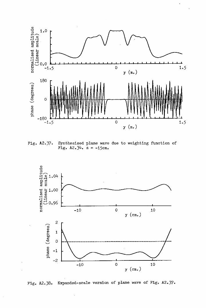
ID'd 1.0;:j.....,~....... IDrlrlPI ro '@ g'd I-lID ro(/) ID....... s::rl .......rorl~,-"O.O 0 1.5o -105s:: y (m; )

180~(/) ~

I~lIDIDHbOID 0'd

il ,"

'-"

ID(/)ro..c:PI -180 • . , . . . •• -,

-1.5 0 1.5y (m.)

Fig. A2.37. Synthesised plane wave due to weighting function ofFig. A2.34. z = -15cmo

ID'd;:j.....,~....... ID 1.04rlrlPlror=: ()ro (/)

~ ~ 1.00(/) ID....... s::rl .......ro rl 6~,-,,0090 -10s::

~ 2(/)IDID 1I-leoID'd 0'-"

ID(/) -1ro.cPI

-2-10

o 10y (cm.)

o 10y (cm.)

Fig. A2.38. Expanded-scale version of plane wave of Fig. A2.37.

180

IDUJ

~P< -180

-1.5

!~ l~ 1\

I' \

• I I • I • • • •

,--....UJIDIDF-IQO

~ 0

o 1.5y (m.)

Fig. A2.39. Synthesised plane wave due to weighting function ofFig. A2.35. z = +15cmo

ID'd 1.10::J+l ,--....or! IDririp<ro@ ~ 1 00'd ~ .IDUJ ID

or! s.:::r-i or!ror-!~ '-"0.90

-100s.:::

4,--....

UJID 2IDF-IQOID 0'd'-"

ID -2UJ

~P< -4

-10

o 10y (cm.)

o 10y (cm.)

Fig. A2.40. Expanded-scale version of plane wave of Fig. A2.39.

-133-

of z # O. The ringing at the edge of the synthesised plane

wave for z = +lScm (Figs. A2.39 and A2.40) is becoming

much more serious although probably still not extending

far enough into the plane wave to cause difficulties.

The set of graphs for a weighting function of 11

points (spacing 5.00) form Figs. A2.41 to A2.47. The

edge of the weighting function is now tapered to -3SdB.

These graphs correspond closely to the sampling criterion

(as modified for the near-field measurement range according

to the analysis of Chapter 2) and it is clear that the

synthesised plane wave is beginning to suffer from the

effects of the overlap.

The final example is of a weighting function of

9 points with a 6.250 spacing (Fig. A2.48) and the

synthesised plane wave (Figs. A2.49 to A2.S4). In this

situation where the sampling criterion is violated, it has

become impossible to synthesise a good plane wave with

severe ripple in evidence for all values of z.

e (degrees)

0 -20 -10 0 10 20X X

~~'-'" X XID -10<0::J~.r-! X X.--I

~ -20<0 X XIDtI.l.r-! -30.--Iro~ X0s:::

-40

180

o

X X X X

IDtI.l

~PI

X X

X XX X

-20 -10 o 10 20e (degrees)

Fig. A2.41. l1-point weighting function for R = 1.0m.

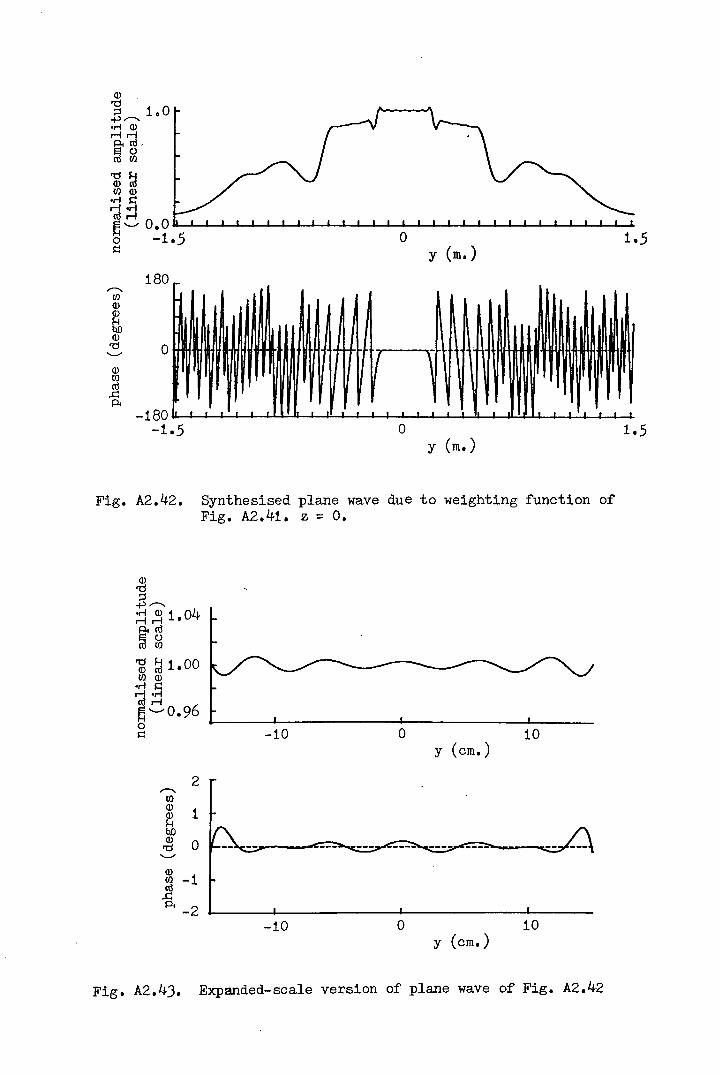
~ 180 ro-

{f1Q)Q)!-lIUlQ)'d 0'--'

Q){f1m..c:P<

-180 . ..-1.5

If ', , . ; ., " -.

o 1.5y (m; )

Fig. A2.42. Synthesised plane wave due to weighting function ofFig. A2.41. z = o.

Q)'d::!.p~;q ~ 1.04P<m@ ~al ~ 1.00{f1 Q)

OM s::r-l OMm";t:i '--' o.960s:: -10

2~{f1Q) 1Q)!-lIUlQ) 0'd'--'

Q)(f.l -1m..c:P< -2

-10

o 10y (cm, )

o 10y (cm.)

Fig. A2.4]. Expanded-scale version of plane wave of Fig. A2.42

Q)"d 1.0;::j+l~OM Q)r-ir;;j~g~~Ul Q)OM 5::r;;j;q~'-" 0.0 0 1.5o -1.55:: (n, )y

~ 180UlQ)Q)1-1eoQ)"d 0'-"

'n fl 11 \Q)Ulro.cPi

-180 I •• r . .-1.5 0 1.5

y (n, )

Fig. A2.44. Synthesised plane wave due to weighting function ofFig. A2.41. z = -15cm.

Q)"d;::j+l~ 4oMQ)1.0~r;;j@ g~ ~ 1.00Ul Q)OM s:::r;;j OM~~0.960 -105::

2~UlQ) 1Q)tbQ) 0"d'-"

Q)Ul -1ro.cPi -2 -10

o 10y (cm.)

o 10y (cm.)

Fig. A2.45. Expanded-scale version of plane wave of Fig. A2.44

ID'd 1.0::l+l r--..r! ID.-Ir-IPtcO@ g~ ~(/) ID.r! !::r;;j .r!~~O.o 0 1.5o -1.5!:: Y (m.)r--. 180(/)IDID~eoID'd 0 A- A'--'

ID

~II \(/)

cO.cPt

-180 I •• I I • .. . ..-1.5 0 1.5

y (m, )

Fig. A2.46. Synthesised plane wave due to weighting function ofFig. A2.41. z = +15cm.

ID'd 1.10::l+l r--..r! ID.-1.-1Ptro

@ g 1 00~ ~ .(/) ID.r! !::r;;j;q~ '--'0.90

-100!::

r--. 4(/)IDID 2~bDID'd 0'--'

ID(/) -2cO..c::Pt

-4-10

o 10y (cm.)

o 10y (cm.)

Fig. A2.47. Expanded-scale version of plane wave of Fig. A2.46.

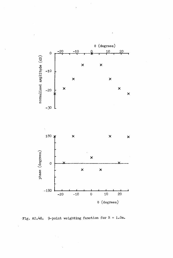
e (degrees)0 10 20

r--.

~'-'"

Q) X X'"d;:j. -10~.r!r-I

~ X X

'"dQ)

X[f.l -20 X.r!r-I Xrot:l0,:::

-]0

180

-180

X Xx

xo ---~-----------------------------------)C-----.

X x

-20 -10 10 20o

e (degrees)

Fig. A2.48. 9-point weighting function for R = 1.0m.

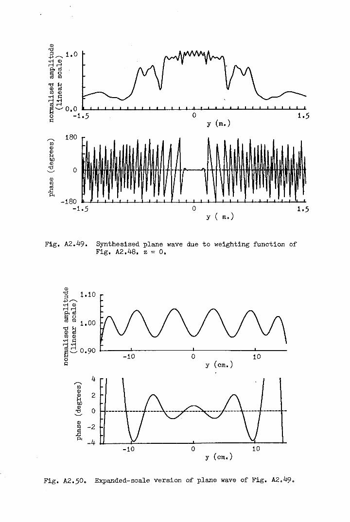
o 1.5y (m.)

.---.. 180[/)Q)Q)1-1tillQ)'ti 0'--"

Q)[/)ro.cPi

.

ft .. t II'~I I I I I I I I I I t t I I t-180

-1.5 oy ( m, )

1.5

Fig. A2.49. Synthesised plane wave due to weighting function ofFig. A2.48. z = o.

Q)'ti i .ro::J~ .---..·rl Q)r-lr-lPiro~ g 1.00al ~[/) Q)·rl $:Ir-I ·rlror-l~ '--"0.90 -100$:I

4.---..[/)Q) 2Q)1-1tillQ) 0'ti'--"

Q)[/) -2ro...c:Pi -4 -10

o 10y (cm.)

o 10y (cm.)

Fig. A2.50. Expanded-scale version of plane wave of Fig. A2.49.

Cl)'d 1.0-E--OM Cl)

~'ida frl~~(fl Cl)OM s::'id;q~ .........0.0

0 1.5o -1.5s:: y (m.)180--(fl

Cl)Cl)

t;b I I ,.Cl) 0 ...'d -

~ \.........

mCl)

v 1nl

~-a I--180 I I • __l • . . . I

-1.5 0 1.5y (m, )

Fig. A2.51. Synthesised plane wave due to weighting fUnction ofFig. A2.48. z = -15cm.

Cl)'d.a-- 1.10OM Cl)

~'ida g~ ~ 1.00(fl Cl)OM s::'id;qt:1 <;» 0.900 -10 0 10s:: y (cm.)

4--(flCl) 2Cl)

t;bCl) 0'd.........Cl) -2~-a -4

-10 0 10y (cm.)

Fig. A2.52. Expanded-scale version of plane wave of Fig. A2.51.

180,.-...I/)Q)Q)~QOQ)~ 0 HtAffi~iHHli.~fRHI"I~~I~HH~fl

y (m.)

Fig. AZ.5J. Synthesised plane wave due to weighting function ofFig. A2.48. z = +15cm.

Q)~ 1.10~.p ............•r-l Q)

~r;;!@ ~~ ~ 1.00I/) Q).r! $:lr-I .r!ror-l~ -- 0.90 -10 0 100$:l

y (cm.)............ 10I/)Q)Q) 5t;bQ)~ 0--Q)I/) -5ro..cPi

-10-10 0 10

y (cm.)

Fig. A2.54. Expanded-scale version of plane wave of Fig. A2.5J.

-134-

Appendix 3: ANGULAR EXTENT OF THE l"lEIGHTINGFUNCTION

Illustrated in this appendix are a few examples of

the effects upon the synthesised plane wave of varying the

angular extent of the weighting function (but keeping the

point spacing constant). This is related to the study of

convolving functions of appendix 1 but, in this case, the

results are after 100 cycles of the iterative optimisation

procedure. The weighting functions are designed to

synthesise a 30cm plane wave from a measurement range of

1.Om. The sample spacing used is 20 in all cases and the

frequency used is 10.OGHz.

The first example, Fig. ~3.1, shows the synthesised

plane wave when the weighting function extends over ±900•

The quality of the synthesised plane wave is very good on

the plane z = 0 but deteriorates for the cases of z = ±lOcm

so that this configuration would prove unacceptable. Little,

if any, improvement, is visible for the case of a weighting

function occupying the range ±600 (Fig. A3.2).

A sudden improvement appears in the quality of the

synthesised plane wave for z # 0 when the range of the

weighting function is halved to ±300 (Fig. A3.3) and this

configuration would certainly be acceptable. A further

improvement is seen in Fig. A3.4 when the range of the

weighting function is once again reduced, this time to

±24°.

A slight deterioration in the quality of the

synthesised plane wave becomes apparent when the range

of the weighting function is ±200, as shown in Fig. A3.5.

The reduction in quality continues with Fig.A3.6(±16°

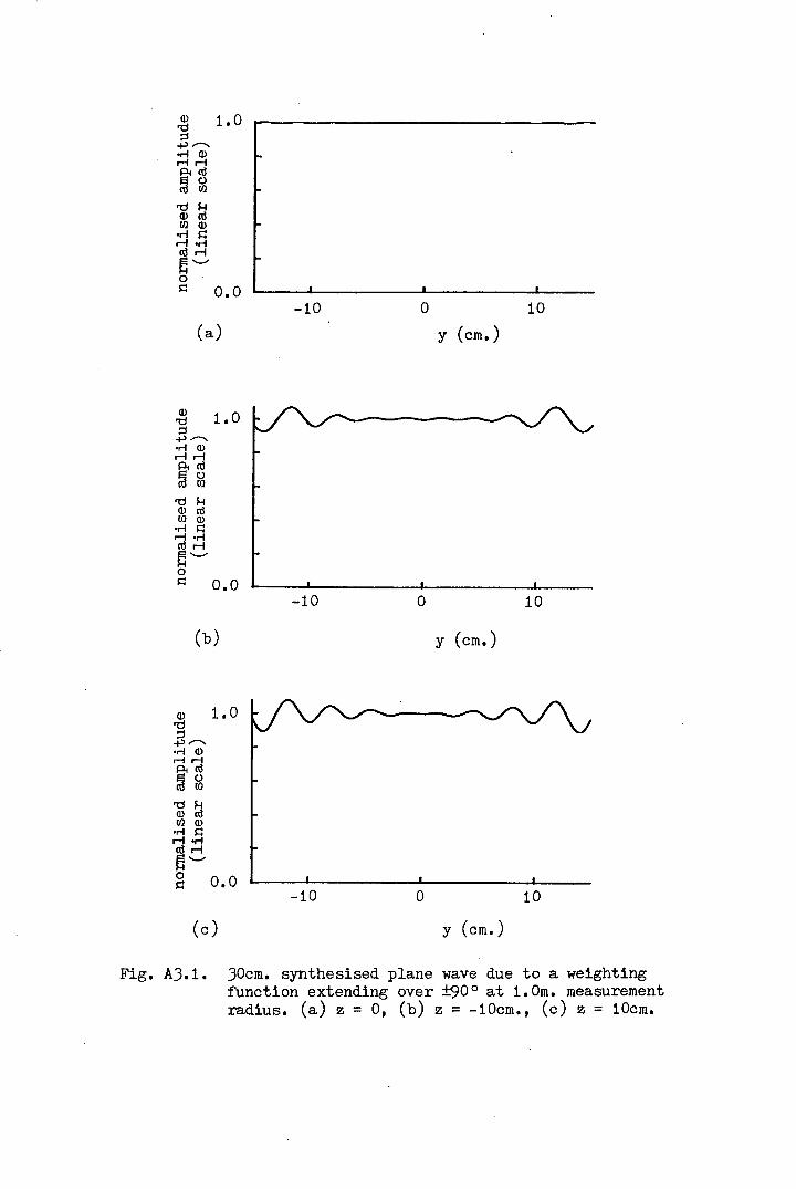
ID 1.0'0;:::s+l ,...._OM IDr-f r-fPim"" ()m [f)

'0 J...lID m[f) IDOM ~r-I OMmr-f~--0~ 0.0

-10 0 10(a) y (cm.)

ID 1.0'0;:::s+l ,...._OM IDr-fr-fPim@ g'0 J...lID m[f) IDOM ~r-f OMmr-f~--0~ 0.0

-10 0 10

(b) y (cm.)

-10 o 10(c) y (cm.)

Fig. AJ.l. JOcm. synthesised plane wave due to a weightingfunction extending over 1900 at 1.0m. measurementradius. (a) z = 0, (b) z = -10cm., (c) z = 10cm.

ID 1.0'd;::l+' .........•.-1 IDr-friAroEl ()ro !Il

'd f..IID ro!Il ID•.-1 ~ri •.-1ror-f~'--'0 0.0~ -10 0 10

(a) y (cm.)

ID 1.0'd;::l+' .........•.-1 IDririAro@ g'd f..IID ro!Il ID•.-1 ~ri •.-1rori~'--'0 0.0~

-10 0 10(b) y (cm.)

ID 1.0'd;::l+' .........•.-1 IDr-friAro@ g'd f..IID ro!Il ID•.-1 ~r-f •.-1rori~'--'0 0.0~

-10 0 10(c) y (cm.)

Fig. A3.2. 30cm synthesised plane wave due to a weightingfunction extending over ±60o at 1.0m. measurementradius. (a) z = 0, Cb) z = -10cm., (c) z = 10cm.

<1> 1.0'd;:l+> ,.-....

or! <1>r-Ir-IAm@ g'd F-l<1> mf/J <1>or! ~r-I or!mr-lEl'--"F-l0~ 0.0

-10 0 10(a) y (cm.)

<1> 1.0'd;:l+> ,.-....

or! <1>r-Ir-IAmEl 0m f/J

~ ~f/J <1>or! ~r-I or!mr-l~'--"0~ 0.0

-10 0 10(b) y (cm.)

<1> 1.0'd;:l+> ,.-....

or! <1>r-Ir-IAm@ s'd F-l<1> mf/J <1>or! ~r-I or!mr-l~'--"0~ 0.0

-10 0 10(c) y (cm.)

Fig. A3.3. 30cm. synthesised plane wave due to a weightingfunction extending over ±30o at 1.0m. measurementradius. (a) z = 0, (b) z = -10cm., (c) z = 10cm.

ID 1.0'd;::!+> ,_..._

o..-l IDMMAm@ g'd I-lID m!I.l ID

o..-l I=lM o..-lmM~'--'0I=l 0.0

-10 0 10(a) y (cm;)

ID 1.0'd;::!+> ,_..._

o..-l IDMMAm@ s'd I-lID m!I.l ID

o..-l I=lM o..-lmM~'--'0I=l 0.0

-10 0 10(b) y (cm;)

ID 1.0'd;::!+> ,_..._

o..-l IDM~~g'd I-lID m!I.l ID

o..-l I=lM o..-lmM~'--'0I=l 0.0

-10 0 10(c) y (cm.)

Fig. AJ.4. JOem. synthesised plane wave due to a weightingfunction extending over 124° at 1.0m. measurementradius. (a) z = 0, (b) z = -10em., (c) z = 10em.

Q) 1.0'd;:1+>~or-I Q)r-Ir-IP-tro@ g'd ~Q) roCD Q)or-I s::r-I .,-iror-l~'--'0 0.0s::

-10 0 10(a) y (cm.)

Q) 1.0'd;:1+>~.,-i Q)r-Ir-IPlro@ g~ ~CD Q).,-i s::r-I .,-iror-l~'--'0 0.0s::

-10 0 10(b) y (cm.)

Q) 1.0'd;:1+>~.r! Q)r-InP-tro@ g'd ~Q) roCD Q).,-i s::r-I -r-iror-l~'--'0s:: 0.0

-10 0 10(c) y (cm, )

Fig. A3.5. 30em. synthesised plane wave due to a weightingfunction extending over 1200 at 1.0m. measurementradius. (a) z = 0, (b) z = -iDem., (c) z = iDem.

Q) 1.0'0;j..p,..--...OM Q)...-1.-1!=lim@ g'OF-!Q) m{/} Q)OM ~...-10Mm.-l~'--'0~ 0.0

-10 0 10Ca) y Ccm.)

(s) Y Ccm, )

Q) 1.0'0;j..p,..--...OM Q)

I=t~r:; ()m {/}'OF-!Q) m{/} Q);q~mM~-.._:.,0 0.0~

-10 o 10(e) y (cm.)

Fig. A3.6. 30cm. synthesised plane wave due to a weightingfunction extending over ±16o at 1.0m. measurementradius. (a) z = 0, (b) z = -10cm., (c) z = 10em.

-135-

weighting function) and Fig. A3.7 (±12° weighting

function.

The effects observed here agree with those predicted

from Chapter 2 where it was shown that an improvement of

plane wave quality would be expected for wider weighting

functions on the plane z = ° but for z ~ 0, defocussing

terms would become serious as the size of the weighting

function became large. Clearly the best range in this

case is ±24° and this value is in fact typically close to

the optimum extent of a weighting function although for

very short range measurements, it sometimes becomes

necessary to increase the angular range a little.

ID 1.0't1~~,......_.r-i IDr-lr-lPiro@ g'g ~If) IDor-i ~r-I .r-iror-l~'-'0~ 0.0

-10 0 10(a) y (cm.)

ID 1.0't1~~,......_.r-i IDr-Ir-IPiro@ g't1 f...IID roIf) ID.r-i ~

~;:1~'-'0~ 0.0

-10 0 10(b) Y (cm.)

ID 1.0't1~~,......_.r-i IDr-Ir-IPiro@ g't1 f...IID roIf) IDor-i ~r-I .r-iror-l~'-'0~ 0.0

-10 o 10(c) y (cm.)

Fig. A3.7. 30em. synthesised plane wave due to a weightingfunction extending over ±12° at 1.0m. measurementradius. (a) z = 0, (b) z = -10em., (c) z = 10em.

-136- .

Appendix 4: THE V-72 IMAGE PROCESSING COMPUTER

Much of the work (particularly the two-dimensional

simulations) described in this thesis was carried out

using the Varian (now Sperry Univac) V-72 image-processing

minicomputer of the University of Sheffield, Department of

Electronic and Electrical Engineering. The system is

described briefly below.

V-72 CPU, l28k (16-bit) memory. Only 32k is availableto a single program at the moment.

- Writeable control store (WCS) - not presently

supported by operating system.

- Hardware floating-point processor (FPP).

- Hazletine VDU.

- Pertec dual magnetic disc drive (4.68 M byte).

- Pertec 9-track magnetic tape deck (800 bpi).

- Racal P-72 digital cassette deck.

- Varian (Sperry) 8-track-paper tape reader (150 cps).

- Facit 8-track paper tape punch (75 cps).

- Mannesmann matrix printer (200 cps).

- Oscilloscope display (locally made) for simple curves.

- C.I.L incremental plotter (O.lmm step, 250 steps per sec).

- Modified Muirhead electrostatic facsimile display(monochrome hard copy intensity display).

- Mk 6 colour T.V display system (locally built).

- Capabilities for use of modem, - direct input of weathersatellite pictures and standard x-y (analogue) plotteroutput.Two of the non-standard peripherals particularly

relevant to the work presented in this thesis will now be

described in a little more detail.

-137-

A4.l C.I.L. Incremental Plotter

The great majority of the graphs presented within this

volume have been plotted on the C.I.L. incremental plotter.

This device is a drum-type plotter with a usable paper width

6f about 32cm, step size of O.lmm and plotting speed in the

region of 250 steps per second. This device is driven

primarily by the "GHOUL" software, written by the present

author, providing quite flexible plotting facilities for

shapes and figures, output of data arrays, axes, graticules,

etc., and callable from FORTRAN programs. In addition,

routines have been written to enable graphical data

produced in the "GHOST" system, operated on the main

University ICL 1906S computer, to be plotted locally

(transfer of data by paper tape).

A4.2 Mk 6 T.V. Display

Probably the most generally important device attached

to the V-72 computer is the locally constructed Mk 6 colour

television display. This is described in more detail by

Thomsit(40) and this outline is therefore very brief.

A displayed picture comprises 256 lines each of 256

display points. The picture is stored in a special memory

within the device. Each point is defined to be at one of

16 grey-scale levels (O-black to IS-peak white) and the

resulting monochrome picture is displayed on a black and

white monitor set. In addition, the Mk 6 hardware and

specially written software allow a colour table to be

defined in which each of the 16 levels is assigned one of

an available 4096 colours (16 levels of red, green and

blue in any combination) and this "false colour" picture

-138-

is displayed on a 3-colour monitor set~

When used with the software written by Dr. A.J.T.

Whitaker, the system provides comprehensive facilities for

displaying and storing pictures using various predefined or

specially designed colour tables, level highlighting, etc.

Combined with the capability of the V-72 computer for data

manipulation, this provides a very powerful tool in the

visualisation of microwave images, field distributions,

etc.

-139-

Appendix 5: SOFTWARE WRITTEN FOR PLANE. WAVE SYNTHESIS

Listed here together with brief descriptions of their

functions are some of the more important items of software

written in the implementation of, or with direct relevance

to, the plane wave synthesis technique and the work

described in this thesis.

PCMP1D The program written for the V-72 minicomputer

(see Appendix 4) for creation of one-dimensional

weighting functions with probe compensation.

Incorporates a large number of features for

investigation of various effects associated with

the plane wave synthesis technique. Described

in more detail in Chapter 1.

SAMPCR Used on the V-72 computer for the investigation

of the sampling criterion described in Chapter 2,

for a single polar (angular) coordinate. Uses

an interval-dividing technique to find the minimum

allowable sampling interval for points within the

significant volume and for various measurement

distances.

FLDPIC)FLDISP)

For displaying, on the Mk 6 T.V. display system,

pictures of the synthesised field distribution due

to a particular weighting function. Run on the V-72

minicomputer.

POLAR1)POLAR2)POLAR3)

For creating the coefficients relating a plane wave

and weighting function for a po1arisation-over-azimuth

scan system, iterating to produce the primary weight-

ing function and producing a printout of the syn-

thesised plane wave. Run on the University of

NPLR1)NPLR2)NPLR3)

CPWTFN

DTRANS

CTRANS

DATAN1

-140-

Manchester Regional Computins Centre, CDC 7600

machine.

For creating the coefficients relating the plane

wave and weighting function for an e1evation-

over-azimuth scan system, iterating to produce

the primary weight'ing function and producing a

printout of the synthesised plane wave. Run on the

CDC 7600

Inputs to the V-72, a primary weighting function

(created by the above programs) on paper tape and,

given details of the measurement geometry, creates

a composite weighting function, stored efficiently

on magnetic tape, corresponding to polarisation-

over-azimuth scan system. At present, only one

prediction polarisation is available but the other

polarisation (as formulated in Chapter 4) will be

incorporated in the next version.

A utility program for creating an appropriately

formatted disc file of a data main scan from an

original file held on magnetic tape (V-72).

A utility program for transferring calibration

scans from magnetic tape to specified disc

files (V-72).When the main scan and calibration scans have

been transferred into their respective V-72 files,

it is useful to have a facility for initially

sorting through the main set and printing out asummary of the data (in terms of maximum, minimum

and mean amplitude and phase values) scan by scan,

DATAN2

DCORR

PRDICT

GETPRD)GETCAL)GETCUT)

COMPAR

-141-

thus facilitating rapid dete~tion of possible

problem areas. In addition to performing this

function, the program enables a detailed comparison

of selected main scan and calibration scan data

by means of graphical output and printout.

For greater thoroughness or where problems of data

are suspected, this second data analysis program

can be called into action to output plots of all

or selected data scans (V-72).

To read a data main scan from its V-72 disc file

and apply a selected correction for slow drift

of amplitude and/or phase before storing it in

another file. Corrections of four types can be

applied in the present version; (a) constant,

(b) Gaussian, (c) cosine, (d) l/¢ type, in any

combination.

The prediction program on the V-72. The composite

weighting function is read from magnetic tape, the

corrected data from disc file and any selected

radial cut (from boresight) of the far-field pattern

is computed and stored on another disc file.

Programs on V-72 for assembling cuts across the

pattern of a far-field prediction, calibration

scan or main scan data for output to a file for use

of the display program.

To display comparisons between cuts across the data.

Used for comparisons of measured near-field calibra-

tion and main scans or predicted and measured far-

field.

-142-

REFERENCES

1. Cheng, D.K., 'On the simulation of Fraunhofer radia-tion patterns in the Fresnel region', IRE Trans.,AP-5, 1957, pp.399-402.

2. Chu, T.S., 'A note on simulating Fraunhofer radiationpatterns in the Fresnel region', IEEE Trans., AP-19,1971, pp.69l-692.

3. Scientific Atlanta Inc., 'The compact range', MicrowaveJournal, 17, October 1974, pp.30-32.

4. Johnson, R.C., Ecker, H.A. and Moore, R.A., 'Compactrange techniques and measurements', IEEE Trans.,AP-17, 1969, pp.568-576.

5. Olver, A.D., 'The practical performance of compactantenna ranges', Proc.Workshop on Antenna TestingTechniques, ESTEC, Netherlands, 1977, pp.129-l33.

6. Wickenden, B.V.A., 'The use of a lens for compactrange measurements', Proc.Seminar on Compact AntennaRanges, RSRE, Malvern, 1980, item 6.

7. Silver, S., 'Microwave Antenna Theory and Design',McGraw Hill, 1949, pp.129-l99.

8. Bennett, J.C., Anderson, A.P., McInnes, P.A. andWhitaker, A.J.T., '~licrowave holographic metrologyof large reflector antennas', IEEE Trans., AP-24,1976, pp.295-303.

9. Strickland, R.N., 'The prediction of antenna far-fieldpatterns from measurements made in the near-fieldregion', University of Sheffield, Department of Elec-tronic and Electrical Engineering, undergraduate thesis,1975.

10. Anderson, A.P., Bennett, J.C., Whitaker, A.J.T. andGodwin, M.P., 'Measurement and optimisation of a largereflector antenna by microwave holography', Proc.International Conference on Antennas and Propagation,London, 1978, pp.128-l3l.

11. Booker, H.G. and Clemmow, P.C., 'The concept of anangular spectrum of plane waves and its relationshipto that of polar diagram and aperture distribution',Proc.IEE, 97(3), 1950, pp.11-17.

-143-

12. Paris, D.T., Leach, W.M. and Joy,. E.B., 'Basictheory of probe-compensated near-field measurements',IEEE Trans., AP-26, 1978, pp.373-379.

13. Joy, E.B., Leach, l"1.M.,'Rodrigue, G.P. and Paris, D.T.,'Applications of probe-compensated near-field measure-ments', IEEE Trans., AP-26, 1978, pp.379-389.

14. Joy, E.B. and Paris, D.T., 'Spatial sampling andfiltering in near-field measurements', IEEE Trans.,AP-20, 1972, pp.253-261.

15. Kerns, D.M., 'Plane wave scattering matrix theory ofantennas and antenna-antenna interactions', Nat.Bureauof Standards, report NBSIR 78-890, 1978.

16. Brown, J. and Jull, E.V., 'The prediction of aerialradiation patterns from near-field measurements',Proc.IEE, 108B, 1961, pp.635-644.

~'

17. Leach, W.M. and Paris, D.T., 'Probe-compensated near-field measurements on a cylinder', IEEE Trans., AP-21,1973, pp.435-445.

18. Borgiotti, G.V., 'Integral equation formulation forprobe-corrected far-field reconstruction from measure-ments on a cylinder', IEEE Trans., AP-26, 1978, pp.572-578.

19. British Aerospace Dynamics, 'Presentation of CNFTAntenna Measurement Facility', Stevenage, 1979.

20. Stratton, J.A., 'Electromagnetic Theory', McGraw Hill,1941, pp.392-423.

21. Wood, P.J., 'Reflector Antenna Analysis and Design',Peter Peregrinus, 1980, pp.36-85.

22. Ludwig, A.C., 'Near-field/far-field transformationsusing spherical wave expansions', IEEE Trans., AP-19,1971, pp.214-220.

23. Larsen, F.H., 'SNIFTC. Spherical near-field transforrna-tio~ program with probe compensation', Experimentalspherical near-field test facility, final report, VII,Technical University of Denmark, Electromagn~ticsInstitute, report R201, 1978.

-144-

24. Martsafey, V.V., 'Measurement of Electrodynamicant~nna parameters by the method of synthesisedapertures', Radio Eng. and Electron.Phys., 13, 1968,pp.1869-1873. --

25. Ludwig, A.C., 'The definition of cross-polarisation',IEEE Trans., AP-2l, 1973, pp.116-ll9.

26. Bracewell, R., 'The Fourier Transform and itsApplications', McGraw Hill, 1965 ..

27. Ludwig, A.C., 'Numerical check on the accuracy ofspherical-wave expansions', Electron.Lett., ~, 1972,pp.202-203.

28. Marvin, A., 'Inadequacy of the Rayleigh range criterionfor superdirective arrays', Electron.Lett., 12, 1976,pp.415-416. --

29. Arsac, J., 'Fourier Transforms and the Theory ofDistributions', Prentice Hall, 1966.

30. Hamming, R.W., 'Numerical Methods for Scientists andEngineers', McGraw Hill, 1962.

31. Abramowitz, M. and Stegun, I.A., (ed) 'Handbook ofMathematical Functions', Dover, 1965.

32. Joy, E.B., 'Maximum near-field measurement errorspecification', Digest, IEEE AP-S, International Symposium,Stanford, 1977, pp.390-393.

33. Bach, H., Lintz Christensen, E., Hansen, J.E., Jensen,F. and Larsen, F.H., 'Facility design and test runs',Experimental spherical near-field test facility, finalreport, I, Technical University of Denmark, Electro-magnetic-Institute, report R208, 1979, pp.25-29.

34. Bennett, J.C., University of Sheffield, private internalcommunication.

35. Jensen, F., 'Computer simulation studies', Experimentalspherical near-field test facility, final report, VI,TICRA ApS, report S-86-03, 1979.

36. Hess, D.W., Willwerth, F.G. and Johnson, R.C. 'Compactrange improvements and performance at 30GHz', Digest,IEEE AP-S, International Symposium, Stanford, 1977,pp.264-267.

-145-

37. Evans, D., 'Microwaves', Radio Co~unication, 52,197,6,p.757.

3S. Silver, S., 'Microwave Antenna Theory and Design',McGraw Hill, 1949, p.34S.

39. Muntanga, E., University of Sheffield, privateinternal communication.

40. Thomsit, D.l., 'Colour display of microwave fields',Electronics and Power, 25, 1979, pp.40S-4l2.