TTooppiicc RReesseeaarrcchh

Integration of Optical and Radar Data to Characterize Land Use of Pollino

National Park

SScchhoollaarrsshhiipp HHoollddeerr

LLiicc.. BBaayyaallaa MMaarrttíínn IIggnnaacciioo.. Master in Emergency Early Warning and Response Space Applications

Mario Gulich Space Studies Institute.

National Commission on Space Activities (CONAE)

Córdoba, Argentina.

TTuuttoorr

Dra. Rosa Maria Cavalli Laboratorio Aereo di Ricerche Ambientali (LARA)

Istituto Inquinamento Atmosferico (IIA)

Consiglio Nazionale delle Ricerche (CNR)

Roma, Italia.

Final Report

Tutor Sign:………………………………………………………………….

SScchhoollaarrsshhiipp HHoollddeerr SSiiggnn::………………………………………………………………………………………………....

1

INDEX

1. ABSTRACT 3

2. DOCUMENT SCOPE 4

3. OBJETIVE 4

4. INTRODUCTION 5

5. BACKGROUND 7

5.1. SYSTHEMATIC APERTURE RADAR (SAR) 7

5.2. Wavelength 8

5.3. Phase 8

5.4. Polarization 9

5.5. Incidence Angle 10

5.6. Scattering Mechanisms 10

5.6.1. Surface and Scattering 10

5.6.2. Double Bounce 11

5.6.3. Penetration 11

5.6.4. Speckle 12

5.6.5. Data Statistics 13

5.6.6. Geometry 13

6. INTERFEROTRETRIC IMAGES 14

6.1. Statistic of the Return 14

6.2. Coherence 15

7. STUDY AREA 17

8. SATELLITE DATA 19

8.1. OPTICAL DATA: GEO-EYE 1 19

8.2. RADAR DATA: COSMO SkyMed 20

2

8.3. DIGITAL ELEVATION MODEL 20

9. METHODS 21

9.1. MULTISPECTRAL IMAGE CLASSIFICATION METHODS 21

9.1.1. Identification of Test Sites 21

9.1.2. Classification of the Very High Resolution Geo-eye Image 22

9.1.2.1.Clasification Pixels Oriented (NDVI thereshold) 23

9.1.2.2.Classification Oriented Object (Segmentation) 24

9.1.2.3.ISODATA Classification with Independent Compenent Analysis 25

9.2. VHR OPTICAL CLASSIFICATION RESULTS 26

9.2.1. Spectral Classification 26

9.2.2. Accuracy Evaluation 27

9.2.3. Analisys Multitemporal between Geo-eye and MIVIS images 29

9.4. VHR RADAR RESULTS 34

9.4.1. Coherence Image Interpretation 34

9.4.2. Integration VHR Optical and Radar Data 35

10. CONCLUSION 37

11. REFERENCES 38

APPENDIX 1_ CORINE Land Cover 2000 41

APPENDIX 2 _ Presentation 44

3

1. ABSTRACT

This study was made on the Basilicata side of Pollino National Park of Pollino National Park, in

the framework of Airborne Laboratory of Environmental Research (LARA) by the availability of

new data set of very high resolution imagery. Therefore, the research proposes was made a

approach of the optical and radar data for land use and land cover mapping.

In this study the land use and cover mapping have been retrieved from the multispectral infrared

visible Geo-eye sensor support by Cosmos SkyMed Spotlight and Himage radar imagery over

the Pollino National Park.

The result over Geo-eye very high resolution data (VHR) allows discriminate with a good

accuracy (up to 2nd

CLC level) the following classes: water course and river bed, bare soil,

woodland and meadow-grassland with a 85 % of averall acurancy and 0.78 of Kappa coefficient.

This methodology can quickly highlight the possible integration between very high resolution

optical and radar data.

4

2. DOCUMENT SCOPE

The aim of the report is to describe the research developed, to characterize land use of Pollino

National Park by integration of optical and radar data in the framework of the SIASGE (Italo-

Argentino System for Emergency Management) scholarship program, managed between CONAE

(Comision Nacional de Actividades Espaciales de Argentina) and ASI (Agenzia Spaziale

Italiana). Tasks were carried out in the Airborne Laboratory of Environmental Research (LARA)

department of the Institute of Atmospheric Pollution (IIA), National Research Council (CNR),

from February up to July 2010 in Rome, Italy.

3. OBJETIVE

• to explore the potential of VHR remote sensing data to support natural vegetation

monitoring.

• to start up an integrated approach to derive Land Use maps by VHR optical and radar

satellite data.

5

4. INTRODUCTION

Over the years, applications of remote sensing have emerged in agriculture, urban planning,

disaster mitigation and monitoring, forestry, hydrology, and operational meteorology among

others. The traditional sources of coarse (>250 m) and moderate resolution (10–250 m) satellite

imagery within the United States have been federal agencies such as NASA and the National

Oceanic and Atmospheric Administration (NOAA). Several commercial companies (e.g. Space

Imaging and Digital Globe) are now providing high spatial resolution (<10 m) satellite data.

With this combination of data types, users have a variety of options to choose the data that best

suits their needs and budget.

Time series of satellite data have long been used to study land-cover changes at global to

regional scales. One of the major challenges is to distinguish between changes linked to

interannual climate variability and land-cover changes induced by anthropogenic processes.

These climatic, geomorphic and anthropogenic processes interact in a complex and dynamic

way, and lead to a wide range of ecosystem responses at different scales (Lambin et al., 2003).

Both a quantification of the magnitude of change as well as a characterization of the change

processes are required to unravel the driving forces of change and their effects on land cover

dynamics (Pan and Bilsborrow, 2005).

However, little is known about the interactions between human land use and the short-term

variability of vegetation activity at regional scales. Until now, the hierarchical organization of

ecosystems, human activities, and their interactions at different levels, from the landscape to the

region, has largely been ignored in remote sensing studies. Processes at these different levels are

interdependent (Paruelo et al., 2001). Factors operating at one level of the hierarchy might

influence processes at a higher or lower level, and should thus be analyzed simultaneously

(Serneels et al., 2007).

As we known, land cover classification and dynamics change are usually performed using the

traditional optical data, although it can suffer from limitations, especially where frequent cloud

6

cover occurs. The increased availability of spaceborne radar imagery offers additional means for

assessing the land use and monitoring their dynamics.

Compared to optical sensors, SAR data does not suffer from the limitations of cloud cover and

darkness and is essentially an all-weather system. The coherence information of ERS SAR

tandem pairs has been successfully used by previous workers for landuse/landcover mapping

(Chatterjee et al., 2002). Moreover, spectral overlaps between fire scars and terrain shadows,

water bodies, and urban areas create substantial difficulties in separating and discriminating land

use classes (Zhang et al., 2000).

In the past few years, the use of SAR remote sensing satellites, such as ERS-1/2, RASARSAT

and JERS-1, has been widely demonstrated in several studies (Strozzi et al, 2000; Engdahl &

Hyyppä, 2003) for land use and urban monitoring application. It has been shown that

multitemporal analysis of SAR data allows monitoring changes in land cover using the

backscatter change intensity.

In this context, the Italian COSMO/SkyMed mission can represent a precious source of

information thanks to the high spatial resolution of the images it acquires, to the very short

revisit time and to the low sensitivity, typical of synthetic aperture radar (SAR) data, to

atmospheric and Sun-illumination conditions. The main novelties of the system are represented

by the possibility to exploit satellite data to generate estimates of soil saturation, at different

space and time scales, to observe the state of rivers and water bodies, and to detect flooded areas,

in any weather and illumination condition. To this end, remote sensing data analysis plays a

crucial and pervasive role in the system; as such data are involved in several processing phases,

i.e., the generation of land-use/land-cover maps by image classification methods, or the

production of change maps by change-detection techniques.

The aims of this study were to explore the potential of VHR remote sensing data to support

natural vegetation monitoring and to start up an integrated approach to derive Land Use maps by

VHR optical and radar satellite data on fragmented landscape of Basilicata area, Italy.

7

5. BACKGROUND

5.1. SYSTHEMATIC APERTURE RADAR (SAR)

To provide a simple definition, Synthetic Aperture Radar (SAR) is a microwave imaging system

that has cloud-penetrating capabilities because it uses microwaves, and it has day and night

operational capabilities because it is an active system.

The imaging radar system composed by an antenna mounted on a platform transmits a radar

signal in a side-looking direction towards the Earth’s surface. The reflected signal, known as the

echo, is backscattered from the surface and received a fraction of a second later at the same

antenna (monostatic radar).

The principle of aperture means the opening used to collect the reflected energy that is used to

form an image (antenna). For RAR systems (real aperture radar) only the amplitude of each echo

return is measured and processed.

The especial resolution of RAR is primarily determined by the size of the antenna used; in fact,

the large the antenna means better spatial resolution. Other determining factors include the pulse

duration (τ), and the antenna bandwidth.

The range resolution is defined as

(1)

Where is the speed of light. The azimuth resolution in defined as

(2)

Where is the antenna length, the distance antenna-abject, and the wavelength.

For systems where the antenna beam width is controlled by the physical length of the antenna,

typical resolutions are in the order of several kilometres. The range resolution of a pulsed radar

system is limited fundamentally by the bandwidth of the transmitted pulse. A wide bandwidth

can be achieved by a short duration pulse.

8

However, the shorter pulse, the lower the transmitted energy and the poorer radiometric

resolution. To preserve the radiometric resolution, SAR systems generate a long pulse with a

linear frequency modulation (or chirp).

The “Interferometric configuration” (Interferometric SAR or InSAR), allows accurate

measurements of the radiation travel path because it is coherent. Measurements of travel path

variations as a function of the satellite position and time of acquisition allow generation of

Digital Elevation Models (DEM) and measurement of contimetric surface deformations of the

terrain.

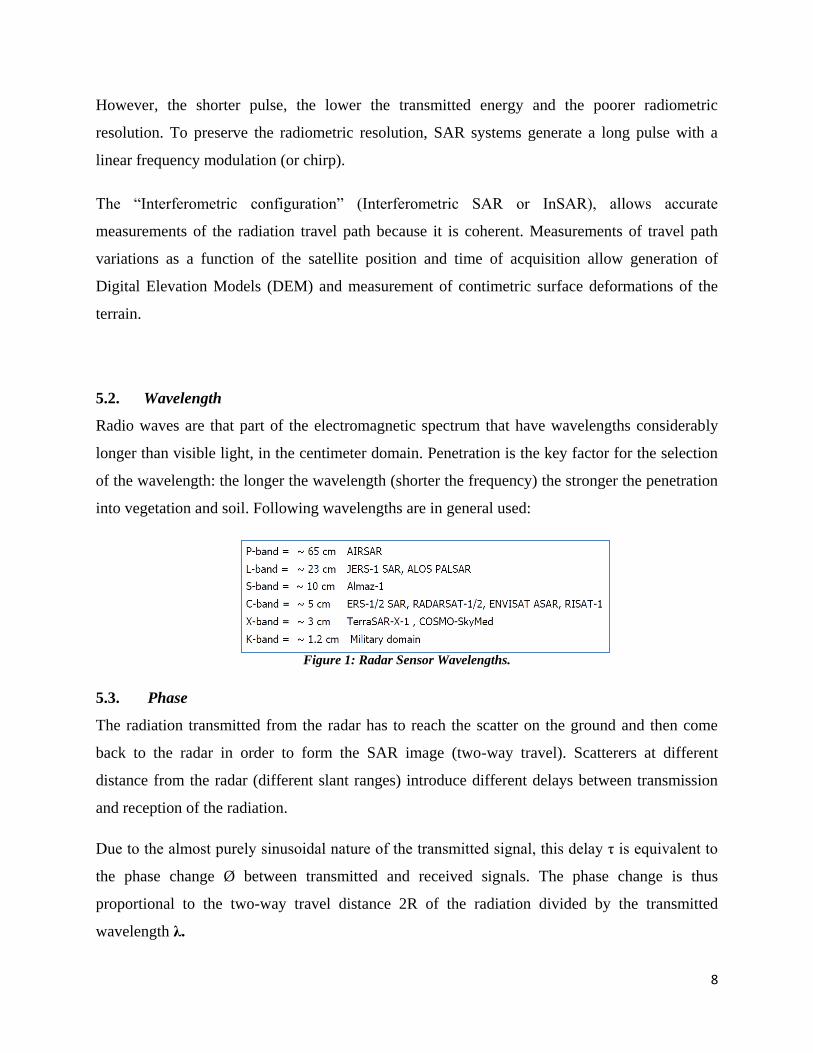
5.2. Wavelength

Radio waves are that part of the electromagnetic spectrum that have wavelengths considerably

longer than visible light, in the centimeter domain. Penetration is the key factor for the selection

of the wavelength: the longer the wavelength (shorter the frequency) the stronger the penetration

into vegetation and soil. Following wavelengths are in general used:

Figure 1: Radar Sensor Wavelengths.

5.3. Phase

The radiation transmitted from the radar has to reach the scatter on the ground and then come

back to the radar in order to form the SAR image (two-way travel). Scatterers at different

distance from the radar (different slant ranges) introduce different delays between transmission

and reception of the radiation.

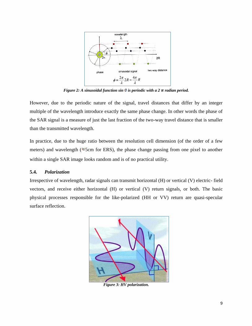
Due to the almost purely sinusoidal nature of the transmitted signal, this delay τ is equivalent to

the phase change Ø between transmitted and received signals. The phase change is thus

proportional to the two-way travel distance 2R of the radiation divided by the transmitted

wavelength λ.

9

Figure 2: A sinusoidal function sin is periodic with a 2 radian period.

However, due to the periodic nature of the signal, travel distances that differ by an integer

multiple of the wavelength introduce exactly the same phase change. In other words the phase of

the SAR signal is a measure of just the last fraction of the two-way travel distance that is smaller

than the transmitted wavelength.

In practice, due to the huge ratio between the resolution cell dimension (of the order of a few

meters) and wavelength ( 5cm for ERS), the phase change passing from one pixel to another

within a single SAR image looks random and is of no practical utility.

5.4. Polarization

Irrespective of wavelength, radar signals can transmit horizontal (H) or vertical (V) electric- field

vectors, and receive either horizontal (H) or vertical (V) return signals, or both. The basic

physical processes responsible for the like-polarized (HH or VV) return are quasi-specular

surface reflection.

Figure 3: HV polarization.

10

5.5. Incidence Angle

The incidence angle () is defined as the angle formed by the radar beam and a line

perpendicular to the surface. Microwave interactions with the surface are complex, and different

reflections may occur in different angular regions. Returns are normally strong at low incidence

angles and decrease with increasing incidence angle.

5.6. Scattering Mechanisms

SAR images represent an estimate of the radar backscatter for that area on the ground. Darker

areas in the image represent low backscatter, while brighter areas represent high backscatter.

Bright features mean that a large fraction of the radar energy was reflected back to the radar,

while dark features imply that very little energy was reflected.

Backscatter for a target area at a particular wavelength will vary for a variety of conditions, such

as the physical size of the scatterers in the target area, the target's electrical properties and the

moisture content, with wetter objects appearing bright, and drier targets appearing dark. The

exception to this is a smooth body of water, which will act as a flat surface and reflect incoming

pulses away from the sensor (these bodies will appear dark). The wavelength and polarization of

the SAR pulses, and the observation angles will also affect backscatter.

5.6.1. Surface and Scattering

A useful rule-of-thumb in analysing radar images is that the higher or brighter the backscatter on

the image, the rougher the surface being imaged. Flat surfaces that reflect little or no radio-

microwave energy back towards the radar will always appear dark in radar images. Vegetation is

usually moderately rough on the scale of most radar wavelengths and appears as light grey in a

radar image.

11

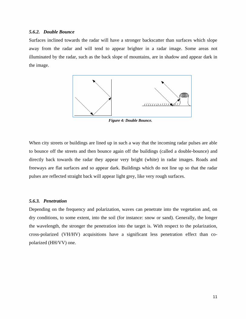
5.6.2. Double Bounce

Surfaces inclined towards the radar will have a stronger backscatter than surfaces which slope

away from the radar and will tend to appear brighter in a radar image. Some areas not

illuminated by the radar, such as the back slope of mountains, are in shadow and appear dark in

the image.

Figure 4: Double Bounce.

When city streets or buildings are lined up in such a way that the incoming radar pulses are able

to bounce off the streets and then bounce again off the buildings (called a double-bounce) and

directly back towards the radar they appear very bright (white) in radar images. Roads and

freeways are flat surfaces and so appear dark. Buildings which do not line up so that the radar

pulses are reflected straight back will appear light grey, like very rough surfaces.

5.6.3. Penetration

Depending on the frequency and polarization, waves can penetrate into the vegetation and, on

dry conditions, to some extent, into the soil (for instance: snow or sand). Generally, the longer

the wavelength, the stronger the penetration into the target is. With respect to the polarization,

cross-polarized (VH/HV) acquisitions have a significant less penetration effect than co-

polarized (HH/VV) one.

12

Figure 5: Penetration.

5.6.4. Speckle

The presence of several scatterers within each SAR resolution cell generates the so-called

“speckle” effect that is common to all coherent imaging systems. Speckle is present in SAR, but

not in optical images. In fact, speckle refers to a noise-like characteristic produced by coherent

systems such as SAR and Laser systems (note: Sun’s radiation is not coherent).

It is evident as a random structure of picture elements (pixels) caused by the interference of

electromagnetic waves scattered from surfaces or objects. When illuminated by the SAR, each

target contributes backscatter energy which, along with phase and power changes, is then

coherently summed for all scatterers, so called random-walk. This summation can be either high

or low, depending on constructive or destructive interference. This statistical fluctuation

(variance), or uncertainty, is associated with the brightness of each pixel in SAR imagery.

When transforming SAR signal data into actual imagery - after the focusing process - multi-look

processing is usually applied (so called non-coherent averaging). The speckle still inherent in the

actual SAR image data can be reduced further through adaptive image restoration techniques

(speckle filtering).

Homogeneous areas of terrain that extend across many SAR resolution cells (for instance, a large

agricultural field covered by one type of cultivation) are images with different amplitudes in

13

different resolution cells. The visual effect is a sort of “salt and papper” screen superimposed on

a uniform amplitude image.

This speckle effect is a direct consequence of the superposition of the signals reflected by many

small elementary scatterers (those with a dimension comparable to the radar wavelength) within

the resolution cell. These signals, which have random phase because of multiple reflections

between scatterers, add to the directly reflected radiation. The resulting amplitude will depend on

the imbalance between signals with positive and negative sign.

5.6.5. Data Statistics

SAR data are composed by a real and imaginary part (complex data), so-called in-phase and

quadrature channels (see figure 6). The amplitude (A) has a Rayleigh distribution, while the

intensity (I) or Power (=A2) has a negative exponential distribution. In single-channel SAR

system the phase provides no information, while the Amplitude (or intensity/Power) is the only

useful information.

Figure 6: Complex Data.

The Intensity or Power data are usually multi-looked by averaging over range and/or azimuth

resolution cells - the so-called incoherent averaging. Fortunately, even multi-looked Intensity

data have a well-known analytic Probability Density Function. In fact, a L-look- image (L is the

number of looks) is essentially for the convolution of L-look exponential distributions.

5.6.6. Geometry

Due to the completely different geometric properties of SAR data in range and azimuth direction,

it is worth considering them separately to understand the SAR imaging geometry. According to

14

this definition, distortions in range direction are large. They are mainly caused by topographic

variations. The distortions in azimuth are much smaller but more complex.

6. INTERFEROTRETRIC IMAGES

6.1. Statistic of the Return

According to the central limit theorem, in order to hold the phase and quadrature components of

the return, and superposition of many independent elementary scatterers, gratings or point

scatterers are independent Gaussian random variables with variance dependent on the terrain

reflectivity. After that, the amplitude of a single pixel in a SAR image has a Rayleigh

distribution. Its amplitude squared or intensity has a Laplacian distribution with mean (Bamler,

1998). The value of in a pixel of horizontal coordinates r (range), a (azimuth) is dependent on

the local reflectivity of the terrain characterized by a non-dimensional parameter, , times the

inverse of sine of the slope of the terrain, to incorporate foreshortening effects that brighten any

surfaces that verge towards the satellite.

The value of decreases for increasing values of the off-nadir angle , and depends on the

terrain cover (Laur, 1998). In order to correctly estimate , it is necessary to average the value

of the intensity (the amplitude squared) over several pixels that should have the same statistics.

(3)

The amplitude of each pixel, being a random variable, in the SAR images is affected by speckle

noise. However, it has to be understood that for repeated acquisitions of a stationary object the

speckle “noise” remains the same, which is different from other kinds of random noise. To

remove this effect, the randomness squares of several neighboring pixels should be averaged.

The formula that gives the dispersion of the estimate, however, depends also on the random

noise superposed on the data that increases the dispersion of the estimate. It is usually given in

terms of the Equivalent Number of Looks (ENL):

15

(4)

Where, number of range looks and number de azimuth looks.

Radiometric resolution is another parameter used to characterize the image quality and therefore

the amount of speckle on the data.

(5)

6.2. Coherence

The principle of SAR interferometry relies on the acquisition of two images of the same scene

with slightly different viewing angles. Usually, after co-registration, the normalized complex

cross- correlation is computed. Its magnitude, called coherence, is an important interferometric

measure, since it provides information about temporal stability and phase difference reliability.

Coherence is a measure of the phase noise of the interferogram, and it has also been successfully

used as a terrain classification parameter. The interferometric phase (i.e., the phase difference

between two images acquired from slightly different sensor positions) contains “geometric

information” from which the three dimensional position of the scatter element can be derived.

Estimation accuracy of the interferometric phase is characterized by the degree of coherence.

Coherence is defined as the absolute value of the normalized complex correlation coefficient:

(6)

in which and denote the first and second complex SAR images respectively, and the

brackets represent the ensemble average, which is estimated by spatial averaging.

The interferometric coherence map provides thematic information that increases the possibility

of discrimination between different lands cover significantly. Coherence is influenced by a

number of independent factors including the time interval between images, the difference in

signals between images due to the different positions in space from which they were acquired,

16

and other factors (Grey et al, 2003). High coherence means no or small changes whereas low

coherence indicates high degree of change. Usually, in coherence maps, high coherence value

areas include residential places, bare soil and deforested areas, whereas low coherence areas

represent the forest, water and some other vegetation. On the other hand, urban areas and

agricultural field show middle to high coherence as they are affected slightly with one day

interval; but, water and forest show low coherence due to the change in the geometric structure

of the scatterers.

Absolute value of the coherence provides a useful measure of the interferogram quality,

excluding random noise; the changes with time of the scattering properties of a target determine

its coherence. In other hand, the amplitude of each pixel of the interferogram is proportional

to the product of the amplitudes , of the two initial images, and its phase is equal to

their phase difference. The SAR image pixels are the realization of random processes and

therefore we can expect the amplitudes of the interferogram to fluctuate severely even in the

most fovourable case of no temporal decorrelation and zero baseline. Therefore, the phase noise

changes from pixel due to different impact of the random noise superposed on the random

amplitudes of the pixels. Pixels with weak returns will show more dispersed interferometric

phase; strong and stable scatterers will yield more reliable phases. In addition, there are

important temporal changes between the two acquisitions: due to the change in the off-nadir

angle and due to random noise.

17

7. STUDY AREA

The Pollino National Park extends over an area of 192.565 hectares, 94.814 ha of which are in

Basilicata region and 97.751 ha in Calabria region. It includes 56 municipalities, 24 in Basilicata

and 32 in Calabria. The study area is the Lucanian side of Pollino National Park, situated in the

south of Basilicata.

Fig.7: Pollino National Park.

The Pollino Park is one of the most important natural Italian Parks both in terms of extension - it

is the widest national Park in Europe - and of naturalistic importance, especially for the presence

of Pinus leucodermis. The agricultural area used in the Lucanian sector of the Park is equal to

about 60 thousand hectares, and more than 55% of which grassland, about 38% fodder crops,

whereas the remaining 7% is for 202 other agricultural uses (ISTAT, 1991). Livestock farming in

the Lucanian area of Pollino Park is scarcely specialized and of small or very small size.

Breeding farms are almost 7.000 (ISTAT, 1991), equal to 57% of the total. Breeding is often

practiced in piedmont areas predominantly between 700 and 900 m above mean sea level.

Vertical migratory herding is still adopted to use high altitude for grazing in summer months;

18

mostly sheep and goat raising farms use grazing as the main form to meet feed requirements of

their herds.

This area exhibits a very complex landscape with various ecosystems ranging from

Mediterranean to Alpine habitats, at elevations varying between 134 and 2266 m a.s.l. Particular

types of vegetation cover can be identified according to the altitude range: (a) up to 500 m a.s.l.,

the natural vegetation coverage is made up of thickets of maquis, and often undergoes an intense

process of replacement with green xeric meadows and Mediterranean shrubby formations due to

human activities; (b) from 500 to 1000–1200 m elevation, the vegetation is characterized

predominantly by woodlands of Turkey oak (Quercus cerris) and by a few groups of mixed oak

woods (mainly composed of oaks such as Quercus pubescens and Quercus cerris); (c) between

1000 to 1800 m altitude, beech (Fagus sylvatica) is the most widespread vegetation type, with

silver firs (Abies alba) also present as small clusters. Together with the beech, these represent a

natural vegetation relict of woodlands that once extended over all these areas; inside

thedeforested areas, wide mesophytic prairies, which are used as pasture land, are often found;

(d) above 1800 m a.s.l., the upper level of the forest belt, xerophytic prairies alternate with

vegetation typical for the carbonate rocks and breccias that form glacial cirques. In this area, the

most common natural vegetation type is the high mountain Mediterranean shrub (juniper

thickets), whereas the most peculiar feature of the park is the Bosnian pine (Pinus leucodermis),

a tree species typical of the Balkan peninsula's flora that is present in just a few areas of Italy.

19

8. SATELLITE DATA

8.1. OPTICAL DATA: GEO-EYE 1

In this study we used the Geo-Eye 1 VHR satellite data. This sensor acquires data in two

different configurations: panchromatic and multispectral. In the multispectral mode it has 4

different bands (see Table 1), from the visible to near-infrared with 1.6 m of spatial resolution, a

revisit time less than three days, swath width of 15.2 km and dynamic range of 11 bit per pixel.

Imaging Mode Panchromatic Multiespectral

Spatial Resolution 0.41 mtrs. GSD at Nadir 1.65 mtrs GSD at Nadir

Spectral Range 450-900 nm 450-520 nm (blue)

520-600 nm (green)

625-695 nm (red)

760-900 nm (near IR)

Swath Width 15.2 km

Off-Nadir Imaging Up to 60 degrees

Dinamic Range 11 bit per pixel

Mission Life Expectation > 10 years

Nodal Crossing 10:30 am

Orbital Altitude 681 km

Revisit Time Less than 3 day

Table 1. Specification parameters of Geo-eye image.

20

For the further land use classification, the whole band set was taken into consideration and an

orthomosaic was built with six Geo-eye 1 images acquired on 06/06/09 and geocoded in the

WGS-84 UTM Projection system (zone 33).

8.2. RADAR DATA: COSMO SkyMed

The Cosmo SkyMed (Constellation of Small Satellites for Mediterranean basin Observation)

radar satellites are the largest Italian investment in Space Systems for Earth Observation funded

by the Italian Space Agency (ASI) and the Italian Ministry of Defense (MoD). They are

constituted by X band radar sensors and are mainly used for civil protection purposes. The main

COSMO characteristics are resumed in Table 2.

For this study we used a set of 8 Cosmo-SkyMed X-band images both in “Spotlight” and

“Stripmap HIMAGE” modes. These images have both a HH polarization with different spatial

resolutions (i.e. the Spotlight images 1m and the Stripmap 3m). The images were acquired

between 13 December 2008 and 3 March 2009 and orthorectified in the WGS-84 UTM

projection system, zone 33.

Table 2. Specification parameters of Cosmo SkyMed image.

8.3. DIGITAL ELEVATION MODEL

Two Digital Elevation data provided by the CNR-IMAA with 6 and 10 meters of resolution were

used to accurately orthorectify both COSMO and Geo-Eye 1 imagery.

Cosmo SkyMed

Spotlight Stripmap ScanSAR

HIMAG

E

Ping

Pong

Wide

Region Huge Region

Polarization Single Single Dual Single Single

Swath width [km x km] 10X10 40X40 30X30 100X100 200X200

Accessible swath ~620 km

Geometric Resolution [m] 1 3 15 30 100

21

9. METHODS

9.1. MULTISPECTRAL IMAGE CLASSIFICATION METHODS

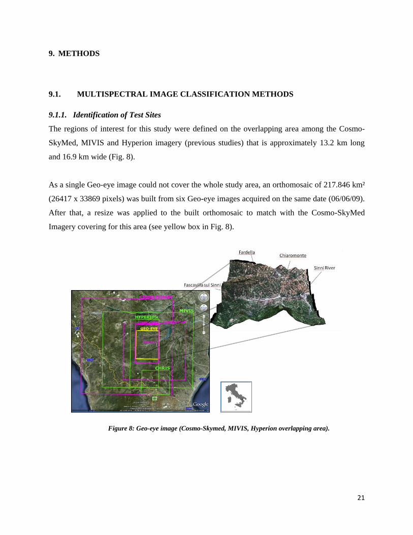
9.1.1. Identification of Test Sites

The regions of interest for this study were defined on the overlapping area among the Cosmo-

SkyMed, MIVIS and Hyperion imagery (previous studies) that is approximately 13.2 km long

and 16.9 km wide (Fig. 8).

As a single Geo-eye image could not cover the whole study area, an orthomosaic of 217.846 km²

(26417 x 33869 pixels) was built from six Geo-eye images acquired on the same date (06/06/09).

After that, a resize was applied to the built orthomosaic to match with the Cosmo-SkyMed

Imagery covering for this area (see yellow box in Fig. 8).

Figure 8: Geo-eye image (Cosmo-Skymed, MIVIS, Hyperion overlapping area).

22

9.1.2. Classification of the Very High Resolution Geo-eye Image

In order to evaluate the potential of Geo-eye data set for mapping land cover and land use in the

chosen study area was implemented the procedure illustrated in figure 8.

The Geo-eye data set was classified at the pixel and object level, and the algorithm performance

and class accuracy were evaluated and compared to establish the best classification results. So, if

the results were not goods the procesure identification started again (loop indentification-

application-validation).

The land covers in the study area were first organized according to the standard legend of the

CORINE Land Cover 2000 (CLC) classification system. In fact, more than 30 ROI’s were

selected and organized according to the standard hierarchical structure of the European Union's

CORINE classification system (Coordination of Information on the Environment) on the Geo-

eye image.

The validation ROI’s were chosen according to the ground truth data, their homogeneous

distribution and with a statistically significative amount of pixels on the Geo-eye image using the

RGB (625-695nm-Red, 520-600nm-Green, 450-520nm-Blue) and NIR (760- 900nm, Near

Infrared) bands combination.

.

23

Flowchart 1: Flow diagram indication steps followed in the method.

At the moment two diferent methodologies were identify on Geo-eye image of 32.000 Km²

(15267 X 8442 pixels) and 2 GB weigth. The first one was based to pixel and the second one to

object. There are a brief description bellow:

9.1.2.1. Clasification Pixels Oriented (NDVI thereshold)

The first step of this methodology consisted in separate the image by mean NDVI thereshold

and the goal of this step was share the relevant information. In fact, the NDVI thereshold was

used to created two mask with and without vegetation. Therefore, the vegetation mask was

created with NDVI value upper 0.68 and the no vegetation mask was created with NDVI value

down 0.68.

The second step was applied the Maximum likelihood algorithm to the image with vegetation

mask. This method allows identified four classes of CORINE: Roof Tiles, Roof Concret, Bare

soil and Water Course-River Bed.

The third step was applied the Isodata algorithm to the image with mask no vegetation and

allows identified tree class of CORINE: Agricultural areas, Woodland, and Meadows/Grassland.

24

The methodology with NDVI thereshold on Geo-eye image of 32.000 Km² (15267 X 8442

pixels) was evaluated by confusion matrix. The Maximum likelihood algorithm has gotten a 73

% overall acurancy and 0.68 Kappa coefficient and the Isodata algorithm has gotten a 90.90 %

averall acurancy and 0.86 Kappa coefficient

9.1.2.2. Classification Oriented Object (Segmentation)

Was employed the eCognition Professional 5.0 version (DP, 2006) software, developed for

Definiens Imaging corporation since 2000, for to carry out the segmentation and classification

oriented object. The classification analysis with this software is based to objects and allow assess

the size, shape, color, texture at the same time. The process time is low because the segmentation

reduces the object number to classify.

The date set image used for the classification of the ortomosaic geo-eye image was performed by

five bands: blue, green, red, near infrared and NDVI index.

The first step in the classification process was performed by the “scale” parameter, which

determines the maximum global segmentation heterogeneity allowed. Is possible to get different

types of segmented images due to the scale parameter can be changed.

The second step was used the Multiresolution Segmentation Mode. The program takes into

account three criteria for segmentation: color, smoothness and compactness. For most cases color

is the most important and which is strongest in the definition of the objects. The color criterion

takes into account the percentage of spectral homogeneity.

The shape and homogeneity are also important in the extraction of objects (e.g., rectangular fit

algorithm). The criteria for segmentation of the image bands were from 0.7 to 0.3 for color and

shape. Within of color option was considered 0.5 for smoothness and compactness.

The third step was classified the image form Nearest Neighbour Algorithm and were chosen

some samples for each class.

25

Unfortunately, the results of this classification cannot be exported and evaluate because they

were not available the software license.

In other hand, the last validated methodology was on a Geo-eye data set of 217.846 km² (26417

X 33869 pixels), with three bans visible and one near infrared of 17 GB weight. Therefore, we

identified a procedure that allow obtain the best result with this image. (see third step in

flowchart 1)

9.1.2.3. ISODATA Classification with Independent Compenent Analysis

The second step was to apply the Independent Components Analysis (ICA) implemented in the

ENVI 4.7 Software. The Independent Component Analysis (ICA) is a multivariate data analysis

process that transforms an input dataset into a new dataset. Hence, transform a set of mixed

signals into components that are mutually independent.

The application of the ICA method was performed to extract some characteristic features from

the VHR image not well distinguishable by using traditional supervised classification methods,

so to obtain a more accurate land use classification.

The third step was to apply the ISODATA classifier on the classified ICA Geo-eye imagery.

The used specification parameters were the followings: Number Class of 20 up to 30, Iterations

10, Change Threshold 5 %, Minimum pixels in class 100, Maximum class Stdv 1 and Maximum

Class Merge Pairs 4.

ISODATA is the acronym of Interactive Self-Organizing Data Analysis Techniques; it is an

unsupervised classifier that calculates class means evenly distributed in the data space then

iteratively clusters the remaining pixels using minimum distance techniques. Each iteration

recalculates means and reclassifies pixels with respect to the new means. Iterative class splitting,

merging, and deleting is done based on input threshold parameters. All pixels are classified to the

nearest class unless a standard deviation or distance threshold is specified, in which case some

pixels may be unclassified if they do not meet the selected criteria. This process continues until

26

the number of pixels in each class changes by less than the selected pixel change threshold or the

maximum number of iterations is reached.

The results of ISODATA algorithm application were compared with a visual review and the

accuracy was checked using the confusion matrix method.

9.2. VHR OPTICAL CLASSIFICATION RESULTS

9.2.1. Spectral Classification

In order obtained the less spurious information to proceed to a spectral classification of classes.

Therefore, to show a spectral separation between selected ROI’s pairs for a given input file.

These values range from 0 to 2.0 and indicate how well the selected ROI’s pairs are statistically

separate. Values greater than 1.9 indicate that the ROI’s pairs have good separability.

Table 3: ROI’s separability.

Bare Soil and Build - Roof 1,71

Water Course-River Bed and Build - Roof 1,81

Water Course-River Bed and Road 1,82

Road and Shadow 1,86

Woodland and Meadow/Grassland 1,86

Water Course-River Bed and Bare Soil 1,94

Build - Roof and Shadow 1,96

Water Course-River Bed and Shadow 1,97

Bare Soil and Woodland 1,97

Woodland and Shadow 1,98

Bare Soil and Shadow 1,99

Water Course-River Bed and Woodland 1,99

Woodland and Road 1,99

Woodland and Build 1,99

Bare Soil and Meadow/Grassland 1,99

Meadow/Grassland and Road 1,99

Water Course-River Bed and Meadow/Grassland 2

Meadow/Grassland and Shadow 2

Meadow/Grassland and Build - Roof 2

27

The results of separability analysis show that ROI’s pairs; like bare soil, roads, and urban areas

has a bad separability. In fact, the spectral responses of the selected classification classes have a

great similarity in the visible and near infrared, due to the limited spectral information of the

sensor. In the Figure 3 it can be seen the spectral behavior for the different class for the

ortomosaic geo-eye image dated 06/06/2009.

Figure 10: Spectral behavior of the Geo-eye image.

9.2.2. Accuracy Evaluation

The classification accuracies was computed by means of a confusion matrix, from which the

overall (OA)(Congalton, 1991) and the Kappa statistics (Cohen, 1960; Montserud & Leamans,

1992) were derived. The OA is the percentage of cases that are correctly allocated, calculated

along the confusion matrix diagonal, while the Kappa coefficient (K) shows how each

classification differs from a random classification of land cover types.

The Kappa statistic is a suitable measure of the accuracy in thematic classification procedures

because it takes into account the entire error matrix instead of simply the diagonal elements, like

the overall accuracy does. The Kappa coefficients and OA values provide a measure of how well

a classification performed with respect to ground-truth data (Michelson et al., 2000). We also

28

used the limit proposed by Foody (2002), who argued that an OA exceeding 85% is considered

good. Although this limit can be considered arbitrary, it provides a useful qualitative benchmark.

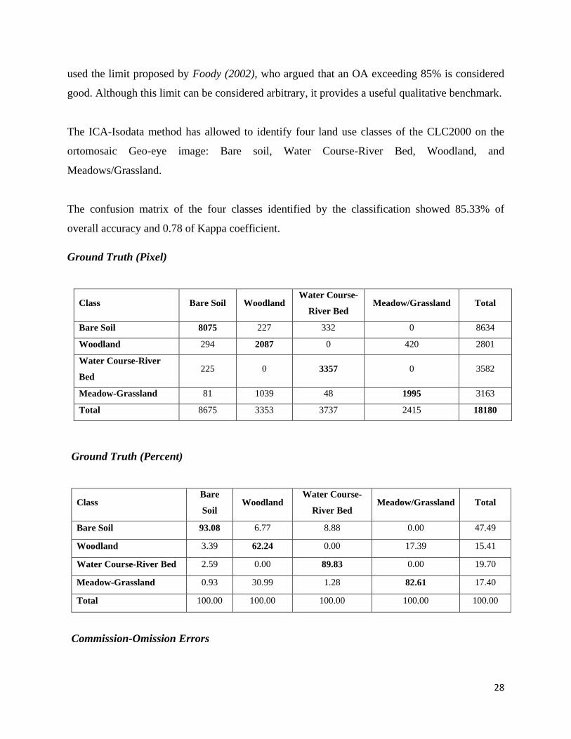
The ICA-Isodata method has allowed to identify four land use classes of the CLC2000 on the

ortomosaic Geo-eye image: Bare soil, Water Course-River Bed, Woodland, and

Meadows/Grassland.

The confusion matrix of the four classes identified by the classification showed 85.33% of

overall accuracy and 0.78 of Kappa coefficient.

Ground Truth (Pixel)

Class Bare Soil Woodland Water Course-

River Bed Meadow/Grassland Total

Bare Soil 8075 227 332 0 8634

Woodland 294 2087 0 420 2801

Water Course-River

Bed 225 0 3357 0 3582

Meadow-Grassland 81 1039 48 1995 3163

Total 8675 3353 3737 2415 18180

Ground Truth (Percent)

Class Bare

Soil Woodland

Water Course-

River Bed Meadow/Grassland Total

Bare Soil 93.08 6.77 8.88 0.00 47.49

Woodland 3.39 62.24 0.00 17.39 15.41

Water Course-River Bed 2.59 0.00 89.83 0.00 19.70

Meadow-Grassland 0.93 30.99 1.28 82.61 17.40

Total 100.00 100.00 100.00 100.00 100.00

Commission-Omission Errors

29

Class Commission

(Percent)

Omission

(Percent)

Commission

(Pixels) Omission (Pixels)

Bare Soil 6.47 6.92 559/8634 600/8675

Woodland 25.49 37.76 714/2801 1266/3353

Water Course-River Bed 6.28 10.17 225/3582 380/3737

Meadow-Grassland 36.93 17.39 1168/3163 420/2415

9.2.3. Analisys Multitemporal between Geo-eye and MIVIS images

The aim of this chapter is see the behavior land use through of 11 years of antropic activity on

Pollino National Park. To detecting any variation on the wood and meadow land was made a

comparation between Geo-eye and Mivis classification.

The airborne MIVIS data were acquired on 9 November 1998, within the framework of the

“Pollino Project” (Cuomo et al., 1999), on the Basilicata side of Pollino National Park. The

MIVIS data cover up to 20,725 ha, with fifteen flight lines oriented NNW–SSE with

approximately 20–25% lateral overlap. MIVIS sensor acquires data in whiskbroom mode with

four spectrometers in the VNIR, SWIR, and TIR ranges, the spatial resolution is 6 -7 m/pixel

depending on the flight altitude with respect to the surface relief. The land cover classification

with the Multispectral Infrared Visible Imaging Spectrometer (MIVIS) airborne hyperspectral

imagery classification was made in 1998.

The overlapping area between the Geo-eye and MIVIS classifications corresponding to a Geo-

eye scene of 1444×2400 pixels and to five contiguous MIVIS strips, was selected as the study

area (shown in fig. 13 a).

30

Figure 11: MIVIS classification up to 5th

CLC

level obtained by applying the MD algorithm

using 13 CORINE classes

Figure 12: Geo-eye classification obtained by ICA-Isodata algorithm

with 4 CORINE classes up to the 2nd

CLC level.

31

(a) (b)

Figure 13. (a) MIVIS woodland classes; (b) Geo-eye woodland classes.

Comparing statistic was done on the woodland class of MIVIS and Geo-eye; The first one

(MIVIS woodland classes) had 55,15 % overall classes with 1.270.741 pixel, and the second one

(Geo-eye woodland classes) had 53,33 % overall classes with 12.102.292 pixel. Hence, the

antropic activity increase in 2.18 % since 1998 ( figure. 13 a-b).

32

9.3. SAR IMAGE PRE-PROCESSING AND PROCESSING METHODS

The Sarscape module implemented in the ENVI 4.7. software was used for the pre-processing of

the 8 Cosmo SkyMed imagery in Spotlight (1 meter) and Himage (2 meter) modes. The images

were acquired between 13 December 2008 and 3 March 2009 and orthorectified in the WGS-84

UTM Projection system, zone 33.

Flowchart 2: Methodological Scheme of Cosmo SkyMed Pre-processing and processing.

The pre-processing of the cosmo SkyMed image was made taking the raw radar data and by

mean the steps showed in the flowchart get a precision product.

The first step was import the Cosmo SkyMed raw data on Sarscape software and transform them

in single look complex image. Images in Single Look Complex format are obtained after

matched filtering in range and azimuth of the raw data and produce a image that contain

amplitude and phase.

33

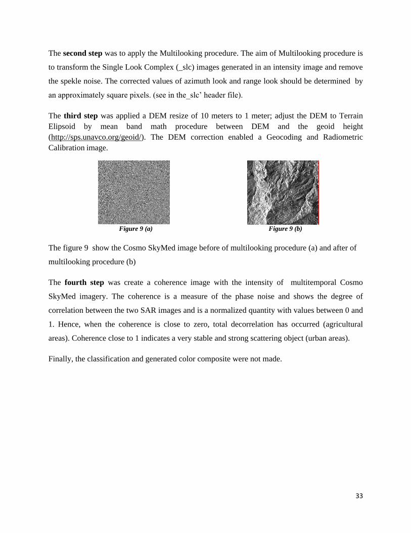
The second step was to apply the Multilooking procedure. The aim of Multilooking procedure is

to transform the Single Look Complex (_slc) images generated in an intensity image and remove

the spekle noise. The corrected values of azimuth look and range look should be determined by

an approximately square pixels. (see in the_slc’ header file).

The third step was applied a DEM resize of 10 meters to 1 meter; adjust the DEM to Terrain

Elipsoid by mean band math procedure between DEM and the geoid height

(http://sps.unavco.org/geoid/). The DEM correction enabled a Geocoding and Radiometric

Calibration image.

Figure 9 (a) Figure 9 (b)

The figure 9 show the Cosmo SkyMed image before of multilooking procedure (a) and after of

multilooking procedure (b)

The fourth step was create a coherence image with the intensity of multitemporal Cosmo

SkyMed imagery. The coherence is a measure of the phase noise and shows the degree of

correlation between the two SAR images and is a normalized quantity with values between 0 and

1. Hence, when the coherence is close to zero, total decorrelation has occurred (agricultural

areas). Coherence close to 1 indicates a very stable and strong scattering object (urban areas).

Finally, the classification and generated color composite were not made.

34

9.4. VHR RADAR RESULTS

9.4.1. Coherence Image Interpretation

The coherence is a measure of the phase noise and show the degree of correlation between the

two SAR images that show a normalized quantity with values between 0 and 1.

This following image is a composition RGB radar data with a coherence image and two Cosmo

SkyMed Himage intensity imagery. Hence, the channel red is the coherence image, in the

channel green the Cosmo SkyMed image of December of 2008 and the channel blue the Cosmos

SkyMed image of March of 2009.

Figure 14: Coherence Image.

The agricultural areas present coherence value close to zero and in the image is showed with the

green color. Therefore, in the agricultural areas a degree of decorrelation exist between both

image

In other hand, the urban areas current a coherence near to one, indicates a very stable and strong

scattering object.

Agricultural areas

Urban areas

35

9.4.2. Integration VHR Optical and Radar Data

The figures 14 (a), (b), (c), (d); bellow shows a example of woodland area on Geo-eye, ICA-

ISODATA classification and Cosmo SkyMed radar imagery.

15 (a): Geo-eye image 3-2-1 bands composition. 15 (b): Geo-eye image 4-3-2 composition .

15 (c): Isodata-ica Classification of Geo-eye image 15 (d): Spotlight Cosmo SkyMed image (03/03/2010)

A visual review on the figure 14 (c) and (d) allow as consider the integration of both data set. In

this sense, the Isodata classification could be useful for support of forest and grassland areas on

Spotlight Cosmo SkyMed image (03/03/2010).

36

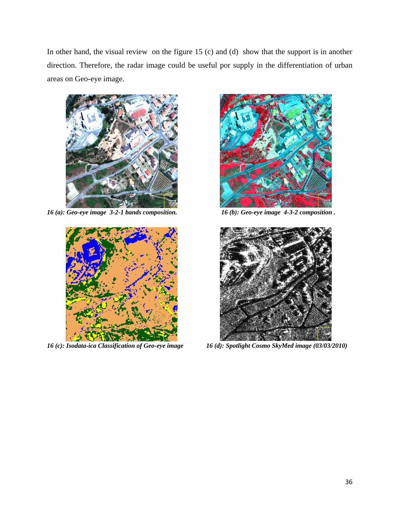
In other hand, the visual review on the figure 15 (c) and (d) show that the support is in another

direction. Therefore, the radar image could be useful por supply in the differentiation of urban

areas on Geo-eye image.

16 (a): Geo-eye image 3-2-1 bands composition. 16 (b): Geo-eye image 4-3-2 composition .

16 (c): Isodata-ica Classification of Geo-eye image 16 (d): Spotlight Cosmo SkyMed image (03/03/2010)

37

10. CONCLUSION

The ICA- Isodata classification for the Geo-eye VHR data allows discriminate with a good

accuracy (up to 2nd

CLC level) the following classes: water course and river bed, bare soil,

woodland and meadow-grassland.

The statistical comparison between forest areas in the classification obtained MIVIS and Geo-

eye imagery can be a useful and cost-effective in the management and monitoring of natural

areas.

The main trouble in order to arrive to an accurate classification on the very high resolution image

was the poor spectral information and complexity of the scene. The diversity of the classes in the

scene increases as the size of the Geo-eye image increases. Therefore, reach higher levels of

CLC on Geo-eye classification is extremely difficult.

The preliminary results highlights the possibility to integrate the optical and radar imagery for

improving the classification/discrimination of urban areas. Hence, the combination of optical

data with radar data source will allow the improvement of the finally classification.

The radar coherence data will be used to try to attain a land cover change map and land use map.

Problems

We had troubles with the availability of the COSMO SkyMed data.

The software licences for the pre-processing and processing of VHR Optical (eCognition) and

Radar Data (Sarscape) were both not available, we used only a trial license for the Sarscape

module.

38

11. REFERENCES

Lambin EF, Geist H, Lepers E. (2003). Dynamics of land-use and land-cover change in tropical

regions. An. Rev. Environ. Resources 28:205–41.

Pan W, Bilsborrow R. (2005). The use of a multilevel statistical model to analyze factors

influencing land use: a study of the Ecuadorian Amazon. Global Planetary Change 47:232–52.

Paruelo J, Burke I, Lauenroth W. (2001). Land-use impact on ecosystem functioning in eastern

Colorado, USA. Global Change Biol. 7:631–9.

Serneels S, Linderman M., and Lambin E. F. (2007). A multilevel analysis of the impactof land

use on interannual land cover change in East Africa. Ecosystems (2007) 10: 402–418

Chatterjee, R.S., Trebossen, H., Rudant, J.P., Fruneau, B., Roy, P.S. (2002). Coherence of

SAR interferometric data as a function of temporal stability of the terrain elements: An

evaluative study to compare the utility of ERS tandem couple and 35-day couple in terrain

analysis. In: Proc. ISPRS Commission VII Symposium on Resource and Environmental

Monitoring, Hyderabad, 2-5 December. pp. 27-31 in sub-section Land Use Planning (on CD-

ROM).

Strozzi, T., Dammert, P., Wegmüeller, U., Martinez, J.M., Askne, J., Beaudoin, A. &

Hallikainen, M. (2000). Landuse Mapping with ERS SAR Interferometry. IEEE Transactions on

Geoscience and Remote Sensing, 38(2), pp766-775.

Engdahl, M.E. & Hyyppä, J.M. (2003). Land-cover Classification Using Multitemporal ERS-

1/2 InSAR Data. IEEE Transactions on Geoscience and Remote Sensing, 41(7), pp1620-1628.

R.S. Chatterjee, S.K. Saha, Suresh Kumar, Sharika Mathew, R.C. Lakhera, V.K. Dadhwal

(2008). ISPRS Interferometric SAR for characterization of ravines as a function of their

density,depth, and surface cover. Journal of Photogrammetry and Remote Sensing.

39

Nicolas Baghdadi, Nathalie Boyer, Pierre Todoroff, Mahmoud El Hajj, Agnès Bégué

(2009).Potential of SAR sensors TerraSAR-X, ASAR/ENVISAT and PALSAR/ALOS for

monitoring sugarcane crops on Reunion Island. Remote Sensing of Environment.

Giorgio Boni, Fabio Castelli, Luca Ferraris, Nazzareno Pierdicca, Sebastiano Serpico and

Franco Siccardi (2007). High resolution COSMO/SkyMed SAR data analysis for civil

protection from flooding events. 1-4244-1212-9

Shengli Huang, Robert L. Crabtree, Christopher Potter, Peggy Gross (2009). Estimating the

quantity and quality of coarse woody debris in Yellowstone post-fire forest ecosystem from

fusion of SAR and optical data Remote Sensing of Environment. RSE-07421.

Robert E. Kennedy, Philip A. Townsend, John E. Gross, Warren B. Cohen, Paul Bolstad,

Y.Q. Wang, Phyllis Adams (2009). Remote sensing change detection tools for natural resource

managers: Understanding concepts and tradeoffs in the design of landscape monitoring projects.

Remote Sensing of Environment 113 -1382-1396.

Floyd M. Henderson and Anthony J. Lewis. (1998). Principles and Applications of Imaging

Radar. ISBN: 0-471-29406-3.11.

Ustin Susan L. (2004). Remote Sensing for Natural Resource Management and Enviromental

Monitoring,.- ISBN: 0-471-31793-4.

Pignatti, Stefano; Cavalli, Rosa Maria; Cuomo Vicenzo; Fusilli, Lorenzo; Pascucci, Simone;

Santini, Federico (2009). Evaluating Hyperion capability for land cover mapping in a

fragmented ecosystem: Pollino National Park, Italy. Remote Sensing of Environment 113 (2009)

622-634.

40

Web site

http://www.geoeye.com/CorpSite/products/services/classification.aspx

http://www.landinfo.com/geo.htm

http://www.e-geos.it/documents.htm

http://www.ecognition.com/products/trial-software

http://www.cosmo-skymed.it/en/index.htm

http://earth.esa.int/EOLi/EOLi.html

http://www.array.ca/nest/tiki-index.php?page=NestSoftwareDownloads

http://www.creaso.com/english/12_swvis/13_envi/SARscape/sarscape.htm

http://europa.eu.int

http://reports.eea.europa.eu/COR0-landcover/en (Corine Land Cover)

41

APPENDIX 1_ CORINE Land Cover 2000

European Union's CORINE (Coordination of Information on the Environment) LandCover2000

(Neumann et al., 2007) classification system (available at http://reports.eea.europa.eu/COR0-

landcover/en).

LAND COVER CLASSES

Class 1: Artificial Areas (Urban)

Class 1.1 Urban fabric

Areas mainly occupied by dwellings and buildings used by administrative/public utilities or

collectivities, including their connected areas (associated lands, approach road network, parking-

lots).

111 Continuous urban fabric

Most of the land is covered by structures and the transport network. Building, roads and

artificially surfaced areas cover more than 80 % of the total surface. Non-linear areas of

vegetation and bare soil are exceptional.

112 Discontinuous urban fabric

Most of the land is covered by structures. Building, roads and artificially surfaced areas

associated with vegetated areas and bare soil, which occupy discontinuous but significant

surfaces.

Class 1.2 Industrial, commercial and transport units

Areas mainly occupied by industrial activities of transformation and manufacturing, trade,

financial activities and services, transport infrastructures for road traffic and rail networks,

airport installations, river and sea port installations, including their associated lands and access

infrastructures. Includes industrial livestock rearing facilities.

42

121 Industrial or commercial units.

Artificially surfaced areas (with concrete, asphalt, tarmacadam, or stabilised,

e.g. beaten earth) without vegetation occupy most of the area, which also

contains buildings and/or vegetation.

122 Road and rail networks.

Motorways and railways, including associated installations (stations, platforms,

embankments). Minimum width for inclusion: 100 m.

Class 1.4 Artificial non-agricultural vegetated areas.

Areas voluntarily created for recreational use. Includes green or recreational and leisure

urban parks, sport and leisure facilities.

Class 2: Agricultural areas

Class 2.1 Arable land.

Lands under a rotation system used for annually harvested plants and fallow lands, which are

permanently or not irrigated. Includes flooded crops such as rice fields and other inundated

croplands.

o 211 Non-irrigated arable land.

o 212 Permanently irrigated land.

Class 2.2 Permanent crops.

All surfaces occupied by permanent crops, not under a rotation system. Includes ligneous crops

of standards cultures for fruit production such as extensive fruit orchards, olive groves, chestnut

groves, walnut groves shrub orchards such as vineyards and some specific low-system orchard

plantation, espaliers and climbers.

43

o 221 Vineyards.

o 222 Fruit trees and berry plantations.

o 223 Olive groves.

Class 2.3 Pastures.

Lands, which are permanently used (at least 5 years) for fodder production. Includes natural or

sown herbaceous species, unimproved or lightly improved meadows and grazed or mechanically

harvested meadows. (231 Pastures).

Class 2.4 Heterogeneous agricultural areas.

Areas of annual crops associated with permanent crops on the same parcel, annual crops

cultivated under forest trees, areas of annual crops, meadows and/or permanent crops which are

juxtaposed, landscapes in which crops and pastures are intimately mixed with natural vegetation

or natural areas. (244 Agro-forestry areas)

Class 3: Bare soils

Land without vegetation cover, with or without atrophic activities.

Class 5: Water courses and water bodies

512 Water bodies.

Natural or artificial stretches of water.

511 Water courses.

Natural or artificial water-courses serving as water drainage channels. Includes canals

and Natural or artificial stretches of water. Minimum width for inclusion: 100 m.

44

APPENDIX 2 _ Presentation

Was made a oral presentation at CNR Montelibretti, Rome; Italy. This seminary was made in

framework of fellowship ASI-CONAE.