Topic 8: The science (or art?) of fitting and interpreting linear regression models

Jeroen Claes

Contents1. Preliminary analyses2. Design choices: Categorical predictor variables3. Design choices: Interactions4. Design choices: How many predictors?5. Design choices: Scaling and centering6. Fitting and interpreting a linear regression model7. Improving on a first model8. The not-so-recommended way: data dredging9. Testing for overfitting and numerical stability with a bootstrap validation10. Wrap-up: How to fit linear regression models in R11. Exercises12. References

1. Preliminary analyses

1. Preliminary analyses (1/3)• We will be working again with the extended version of the dataset by Balota et al.

(2007) that we have seen before (data provided by Levshina, 2015)– Word– Length: word length– SUBTLWF: normalized word frequency– POS: part-of-speech– Mean_RT: Mean reaction time

• Research question:– To what extent and how do word length, word frequency, and part-of speech

condition subjects’ reaction times in a lexical decision task?library(readr)library(dplyr)library(ggplot2)

dataSet <- read_csv("http://www.jeroenclaes.be/statistics_for_linguistics/datasets/class7_Balota_et_al_2007.csv")glimpse(dataSet)

## Observations: 880## Variables: 5## $ Word <chr> "rackets", "stepmother", "delineated", "swimmers", "um...## $ Length <int> 7, 10, 10, 8, 6, 5, 5, 8, 8, 6, 8, 12, 8, 6, 7, 3, 3, ...## $ SUBTLWF <dbl> 0.96, 4.24, 0.04, 1.49, 1.06, 3.33, 0.10, 0.06, 0.43, ...## $ POS <chr> "NN", "NN", "VB", "NN", "NN", "NN", "VB", "NN", "NN", ...## $ Mean_RT <dbl> 790.87, 692.55, 960.45, 771.13, 882.50, 645.85, 760.29...

1. Preliminary analyses (2/3)• Recall that before you can even think of fitting a linear regression model, you have to:

– Investigate the distributions of all of your variables:• What are their central tendencies?• What is their dispersion?• Are there any outliers?

– Examine the relationship of the independent variables to your dependent variable:

• Are they linear?• Are they homeoskedastic?

– Examine the relationships between each of your individual predictors:• Are they correlated? To which extent?

• After investigating all of this, you can begin to fit your model

1. Preliminary analyses (3/3)• From Topic 7 we know that the data has some issues that need to be corrected:

– Heteroskedasticity– Outliers

• These can be corrected with the following codelibrary(car)# OutliersdataSet<-dataSet[abs(scale(dataSet$Mean_RT)) <= 2, ]dataSet<-dataSet[abs(scale(dataSet$Length)) <= 2, ]dataSet <- dataSet[abs((dataSet$SUBTLWF-median(dataSet$SUBTLWF))/mad(dataSet$SUBTLWF)) <= 3.5, ]# SUBTLWF needs a log-transformationdataSet$SUBTLWF<-log(dataSet$SUBTLWF)# Define an initial regression modelmod<- lm(Mean_RT ~ Length + SUBTLWF + POS, data=dataSet)# Overly influential observationsindices <-row.names( influencePlot(mod))

indices <-as.numeric(indices)dataSet <- dataSet[-indices, ]# HeteroskedasticitytestValues <- boxCox(mod, plotit=FALSE)exponent <- testValues$x[which.max(testValues$y)]dataSet$Mean_RT_transformed <- dataSet$Mean_RT^exponent

2. Design choices: Categorical predictor variables

2. Design choices: Categorical predictor variables (1/4)• Categorical variables can be handeled in different ways in regressions, this is called

contrasts• The default contrasts assume that the first level of a factor is the control condition and

that the second level is the treatment condition• This is called treatment contrasts• Only for the second level we get regression coefficients, which express the deviation

with respect to the first level• This makes sense in many experimental settings, where there is a clear

reference/baseline and a trial condition– E.g., Primed condition is compared to unprimed condition in structural priming

experiment• Treatment contrasts make less sense for most corpus-based designs

2. Design choices: Categorical predictor variables (2/4)• Sum contrasts are often more useful for corpus-based designs

• With sum contrasts the coefficients for each factor level express the deviation that is caused by that factor level with respect to the global mean of the dependent variable

• We get coefficients for all factor levels, minus the last level• The sum of the coefficients is zero• We can calculate the coefficient for the missing level by substracting the sum of the

coefficients from zero• To specify human-readable sum contrasts, we can set the option contr to

c("contr.Sum", "contr.Poly"). This requires the car packagelibrary(car)options(contr=c("contr.Sum", "contr.Poly"))

2. Design choices: Categorical predictor variables (3/4)• In other cases the predictor levels imply a particular ordering

– E.g., First case, second case, third case…• For this type of categorical predictor, you should specify ordinal contrastslibrary(car)options(contr=c("contr.Poly"))

2. Design choices: Categorical predictor variables (4/4)• With the options command we specify the global contrasts function• In some cases, it may make sense to specify e.g., treatment contrasts for one variable,

sum contrasts for another, and ordinal contrasts for yet another predictor• In these cases, you will have to set the contrasts for each variable individually with the

contrasts functioncontrasts(dataSet$Word) <- contr.Sum(dataSet$Word)

3. Design choices: Interactions

3. Design choices: Interactions (1/8)• Plotting of the relationships of your variables to the dependent variable is essential:

– To catch any non-linear relationships early on– To spot outliers early on– To find interactions between variables:

• The term interaction describes a situation where there is partical co-dependence between variables, i.e., the effect of a particular predictor varies along the values of a second variable

• Consider e.g., a priming experiment. It may be the case that female students are less susceptible to priming than male students or it may even be that the effect is reversed

• If your dataset is large enough, these interactions may greatly improve your model

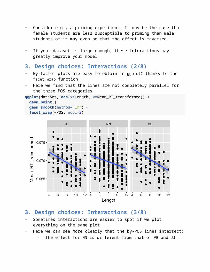
3. Design choices: Interactions (2/8)• By-factor plots are easy to obtain in ggplot2 thanks to the facet_wrap function• Here we find that the lines are not completely parallel for the three POS categoriesggplot(dataSet, aes(x=Length, y=Mean_RT_transformed)) + geom_point() + geom_smooth(method="lm") + facet_wrap(~POS, ncol=3)

3. Design choices: Interactions (3/8)• Sometimes interactions are easier to spot if we plot everything on the same plot• Here we can see more clearly that the by-POS lines intersect:

– The effect for NN is different from that of VB and JJggplot(dataSet, aes(x=Length, y=Mean_RT_transformed, group=POS, color=POS, fill=POS)) + geom_point() + geom_smooth(method="lm", se= FALSE)

3. Design choices: Interactions (4/8)• To explore the interactions between two continous variables, we may discretize one of

them• The ntile function in the dplyr package breaks up the distribution in n bins• If we use n=4, we get 4 quartile groups, which will help us identify interactions• In statistics/machine learning, this is called binning• Since Length has few unique values, we could equally have plotted the values without

binningdat <- dataSet %>% mutate(Length_bins=ntile(Length, 4))

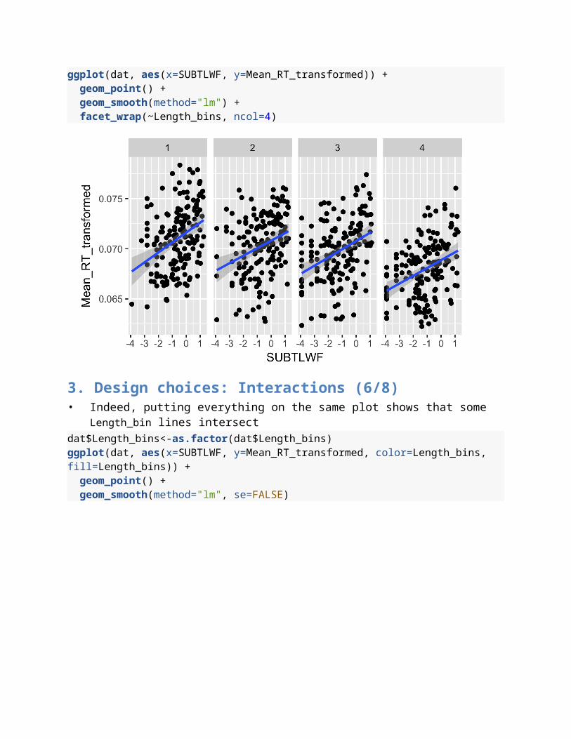
3. Design choices: Interactions (5/8)• The plot appears to reveal an interaction between SUBTLWF and Length as the line for

the first Length quartile is steeper than the othersggplot(dat, aes(x=SUBTLWF, y=Mean_RT_transformed)) + geom_point() + geom_smooth(method="lm") + facet_wrap(~Length_bins, ncol=4)

3. Design choices: Interactions (6/8)• Indeed, putting everything on the same plot shows that some Length_bin lines

intersectdat$Length_bins<-as.factor(dat$Length_bins)ggplot(dat, aes(x=SUBTLWF, y=Mean_RT_transformed, color=Length_bins, fill=Length_bins)) + geom_point() + geom_smooth(method="lm", se=FALSE)

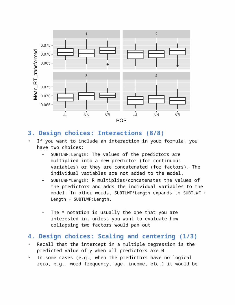
3. Design choices: Interactions (7/8)• Recall that if you want to compare the scores of a continuous variable across groups

identified by one or more categorical variables, boxplots are the method of choice• To spot interactions, facetted boxplots may be very helpful: if the differences between

the medians are more acute or the trend becomes reversed, there may be a relevant interaction there

dat <- dataSet %>% mutate(Length_bins=ntile(Length, 4))ggplot(dat, aes(x=POS, y=Mean_RT_transformed)) + geom_boxplot() + facet_wrap(~Length_bins)

3. Design choices: Interactions (8/8)• If you want to include an interaction in your formula, you have two choices:

– SUBTLWF:Length: The values of the predictors are multiplied into a new predictor (for continuous variables) or they are concatenated (for factors). The individual variables are not added to the model.

– SUBTLWF*Length: R multiplies/concatenates the values of the predictors and adds the individual variables to the model. In other words, SUBTLWF*Length expands to SUBTLWF + Length + SUBTLWF:Length.

– The * notation is usually the one that you are interested in, unless you want to evaluate how collapsing two factors would pan out

4. Design choices: Scaling and centering (1/3)• Recall that the intercept in a multiple regression is the predicted value of y when all

predictors are 0• In some cases (e.g., when the predictors have no logical zero, e.g., word frequency, age,

income, etc.) it would be more meaningful to have the intercept correspond with the predicted y-value when all predictors are at their mean value

• This is what scaling and centering does: it scales the predictors and the response variable linearly such that their means are 0

• We speak of standardized coefficients when they were calculated for scaled/centered X and Y variables

4. Design choices: Scaling and centering (2/3)• To scale a predictor or the dependent variable, we can use

as.numeric(scale(predictor))dataSet$Length<- as.numeric(scale(dataSet$Length))

4. Design choices: Scaling and centering (3/3)• Scaling is very useful when you have multiple numeric predictors that are on different

scales, in which case it makes comparing the coefficients more straightforward• The only disadvantage is that the units of the regression coefficients are less easily

translatable to real-world units, as they are on the Z-score scale (rather than on the scale of the Y-axis)

• Scaling also reduces the degree of correlation between interaction variables and the predictors they are made up of

#Without scalingcor(dataSet$Length, dataSet$Length*dataSet$SUBTLWF)

## [1] -0.3209568

#With scalingcor(scale(dataSet$Length), scale(dataSet$Length)*scale(dataSet$SUBTLWF))

## [,1]## [1,] 0.02184578

5. Design choices: How many predictors/interactions?

5. Design choices: How many predictors/interactions? (1/2)• At this point, we know our data in and out, we have considered the relationships of our

independent variables to the dependent variable, we have excluded outliers, and we have looked for interactions

• With this information, we can specify a first regression model• We use this model to validate the regression assumptions and to get a first impression

of which predictors condition the dependent variable

5. Design choices: How many predictors/interactions? (2/2)• It is important that you do not include more predictors in the model than your data

can support• Otherwise you will run into overfitting:

– Your model does not learn the generalizations in your data. Instead, it picks up on the white noise

– This results in a model that fits the data well, but fails to generalize to new datasets

• As a general rule of thumb, you will want 10-15 observations (rows in your data.frame) per coefficient in your model (a factor with 2 levels counts as 2 coefficients)

• Here we have 9 coefficients, and 660 data points, so we’re well in the clear

6. Fitting and interpreting a linear regression model

6. Fitting and interpreting a linear regression model (1/6)• We define the model as follows• This would be the point where we check all the regression assumptions carefullymod1 <- lm(Mean_RT_transformed ~ Length + SUBTLWF + POS + POS * Length + SUBTLWF*Length, data=dataSet)

6. Fitting and interpreting a linear regression model (2/6)• We can inspect the results by calling summary on the model objectsummary(mod1)

## ## Call:## lm(formula = Mean_RT_transformed ~ Length + SUBTLWF + POS + POS * ## Length + SUBTLWF * Length, data = dataSet)## ## Residuals:## Min 1Q Median 3Q Max ## -0.0073219 -0.0019512 0.0000778 0.0018924 0.0075542 ## ## Coefficients:## Estimate Std. Error t value Pr(>|t|) ## (Intercept) 7.526e-02 1.122e-03 67.091 < 2e-16 ***## Length -6.125e-04 1.338e-04 -4.579 5.6e-06 ***## SUBTLWF 1.144e-03 3.937e-04 2.906 0.00379 ** ## POSNN -1.700e-03 1.239e-03 -1.372 0.17053 ## POSVB 1.650e-03 1.438e-03 1.147 0.25174 ## Length:POSNN 2.218e-04 1.461e-04 1.519 0.12937 ## Length:POSVB -1.155e-04 1.711e-04 -0.675 0.50008 ## Length:SUBTLWF -3.971e-05 4.601e-05 -0.863 0.38838 ## ---## Signif. codes: 0 '***' 0.001 '**' 0.01 '*' 0.05 '.' 0.1 ' ' 1

## ## Residual standard error: 0.002828 on 652 degrees of freedom## Multiple R-squared: 0.2454, Adjusted R-squared: 0.2373 ## F-statistic: 30.29 on 7 and 652 DF, p-value: < 2.2e-16

6. Fitting and interpreting a linear regression model (3/6)• The Estimate column contains the coefficients:

– Coefficients are on the same scale as the y-value. Since we applied a transformation to our y-value, they are on this exponentiated scale

– For each unit increase in Length, subjects need on average 6.12529110^{-4} units less compared to the baseline of 0.0752576 units

– When the POS is a verb, they need 0.00165 units more• The Std Error provides the standard error of the estimates. Larger standard errors

point to less certainty when it comes to the estimates• The t value column provides the t-statistic on which the p-value is based• The Pr(>|t|) column gives you the p-value associated with the effect

6. Fitting and interpreting a linear regression model (4/6)• Interpreting the interaction terms is a bit more complicated:

– The value 2.217902510^{-4} that is reported for Length:POSNN indicates that the normal effect of -6.12529110^{-4} units per unit increase in Length has to be added up with 2.217902510^{-4}, yielding an effect of -3.907388510^{-4} units for Length when the word is a noun.

– The value -3.97141610^{-5} that is reported for indicates that, as we move along the values of Length, the effect of SUBTLWF changes. For each increase in Length, the effect of SUBTLWF decreases with -3.97141610^{-5} units.

6. Fitting and interpreting a linear regression model (5/6)• At the bottom, we find a couple of summary statistics:

– Residual standard error:• Standard error of the residuals, how much variability do the residuals

display. Lower is better.– 652 degrees of freedom:

• Degrees of freedom in your model, which reflects the number of predictor values in your model

– Multiple R-squared: % of variance that is explained by the model. Here we find that the model only accounts for 25% of the variance.

• 0 indicates a useless model, as the model would have as much success when it would always predict the mean value of Y.

• 1 indicates a perfect model, which provides correct predictions for each individual value

6. Fitting and interpreting a linear regression model (6/6)• At the bottom, we find a couple of summary statistics:

– Adjusted R2:• The R2 squared value that is adjusted for the number predictors in the

model and the predictor-to-observations ratio• This R2 decreases when the model includes too many useless predictors

or when there are too few observations

– F-statistic: The ratio of the variance explained by the model to the residual variance. The p-value expresses the chance of observing the F-ratio by chance, which shows us that our model as a whole performs significantly better than chance

7. Improving on a first model

7. Improving on a first model (1/5)• With this initial model, we can try to obtain a more parsimonious model by applying

Occam’s Razor:– We exclude predictors that do not contribute significantly to improving the fit

of the model– We should look for predictors that have small effect sizes and high p-values,

exclude those one at a time and compare the fit of the model with the initial model or a previous better-fitting model

7. Improving on a first model (2/5)• To compare the fit, we calculate Akaike's Information Criterion, a measure

that expressses the tradeoff between model fit and model complexity:– If a model has many ‘useless’ predictors, its AIC rises

• If a model without a predictor has a AIC value that is at least two units lower than a model with the predictor, there is more evidence in favor of the simpler model than there is for the more complex model (Burnham & Anderson, 2008: 70)

7. Improving on a first model (3/5)• The summary shows that the POS variable and its interaction with SUBTLWF have the

smallest effect sizes and p-values higher than 0.05• These terms appear to be good candidates to exclude.• As a rule of thumb, you will want to start with interactions before you remove main

effectsmod2 <- lm(Mean_RT_transformed ~ Length + SUBTLWF +POS + Length*SUBTLWF, data=dataSet)mod3<- lm(Mean_RT_transformed ~ Length + SUBTLWF +POS + Length*POS, data=dataSet)

mod3 <- lm(Mean_RT_transformed ~ Length + SUBTLWF + POS, data=dataSet)mod4 <- lm(Mean_RT_transformed ~ Length + SUBTLWF, data=dataSet)

7. Improving on a first model (4/5)• If we now calculate the AIC statistic for mod1 and mod2 we may evaluate whether the

model without POS has a better fit:– AIC(mod1) - AIC(mod2) yields a difference of -2.5391909 units.– This means that the AIC of mod2 is almost three units higher– This implies that there is substantially more evidence in favor of the model

with the interaction POS*Length

7. Improving on a first model (5/5)• If we now calculate the AIC statistic for mod1 and mod3 we may evaluate whether the

model without POS*SUBTLWF has a better fit:– AIC(mod1) - AIC(mod3) yields a difference of -0.9177945 units.– This implies that there is not substantially more evidence in favor of the model

without the interaction POS*Length– Quite unsurprisingly, dropping POS and all of its interactions does not receive

much support either

8. The not-so-recommended way: data dredging/stepwise model fitting

8. The not-so-recommended way: data dredging/stepwise model fitting (1/5)• It is still rather common in (socio)linguistics to find what is called stepwise

variable selection or data dredging (e.g., Rbrul, GoldVarb, dredge in the MuMIn package)

• Without much analysis/theoretical reflection/hypotheses, a bunch of predictors are fed to an algorithm that builds up a model from scratch and then eliminates predictors one at a time to obtain the most parsimonious fit automatically

8. The not-so-recommended way: data dredging/stepwise model fitting (2/5)• “Stepwise variable selection has been a very popular technique for many years, but if

this procedure had just been proposed as a statistical method, it would most likely be rejected because it violates every principle of statistical estimation and hypothesis testing” (Harrell, 2015: 67)

8. The not-so-recommended way: data dredging/stepwise model fitting (3/5)• These are the most important problems of stepwise regression according to Harrell

(2015: 67-68):– In the vast majority of the cases, the true predictor is not selected by the

dredging process– The R2 values of model derived with stepwise regression are higher than they

should be– The method violates just about every assumption of statistical hypothesis

testing: hypothesis tests are performed without prespecified hypotheses and null hypotheses.

– The method yields overconfident estimates of the generalizeability of the results from the sample to the population (standard errors for coefficents that are biased low and confidence intervals for effect estimates that are falsely narrow)

– The method yields p-values that are too small– It overestimates the effects of predictors (it provides regression coefficients

that are biased high)– Rather than solving problems caused by multicollinearity, variable selection is

made arbitrarily when there are collinear predictors in the model– It allows us to not think about the problem

8. The not-so-recommended way: data dredging/stepwise model fitting (4/5)• The last one may be the most severe problem of all, as stepwise regression gives the

analyst a false sense of security:– “If a rigorous automatic method says that this is the best model, it can only be

the absolute truth”– If we have no theoretical backing, we are terribly exposed to spurious

correlations and effects that make no sense at all– Regression analysis is a form of inferential statistics. Inferential statisitcs

without specific hypotheses to test is a big NO-NO

8. The not-so-recommended way: data dredging/stepwise model fitting (5/5)• R includes functions to do the variable selection process automatically

– drop1– step

• Consult Levshina (2015:149-151) or Field et al. (2012: 264-266) for instructions on how to use them, but I would not recommend automated variable selection

9. Testing for overfitting and numerical stability with a bootstrap validation

9. Testing for overfitting and numerical stability with a bootstrap validation (1/6)• The model output gives you information on the effect sizes of each of the invidual

predictors and their statistical significance• If the model overfits, this information will be worthless, because it will fail to

generalize to new data• To exclude overfitting you should perform a bootstrap validation

9. Testing for overfitting and numerical stability with a bootstrap validation (2/6)• The best way to evaluate if our model overfits/generalizes would be to collect new

data, apply the model to that data and see how well the coefficients correspond• Unfortunately, this is not an option in most cases• However, we can mimic a new dataset drawn from the same population by re-

sampling the same amount of data from our original sample with replacement• This means that we may randomly select the same observations more than once• If we repeat this procedure a large number of times (>= 1,000 times), we will

effictively have evaluated our model on a large number of potentially very different samples

• This comes close to collecting a large number of new samples• In principle, you could do this for any statistic (e.g., mean, median,…)

9. Testing for overfitting and numerical stability with a bootstrap validation (3/6)• Bootstrap validation requires some intermediate-level programming in R• To be able to collect the results in a tidy way, we need the broom package• The idea is the following:

– We are going to create a loop that runs 1,000 times– For each iteration of this loop we are going to sample 660 random observations

from our data (the same amount as there is in the original sample)– With this bootstrap sample we will compute the model again– We store the output of lm in a dataframe with the tidy function of the broom

package– We glue everything together by columns in a single data.frame at the end

library(broom)library(dplyr)bootstrap <- lapply(1:1000, FUN=function(x) { #'lapply' loops

indices <- sample(1:nrow(dataSet), nrow(dataSet), replace = TRUE) # Create indices dat <- dataSet[indices, ] #Sample indices from our data mod <- lm(Mean_RT_transformed ~ Length + SUBTLWF + POS + SUBTLWF*POS, data=dat) #Run the model return(tidy(mod)) #Convert to a data.frame and return }) %>% bind_rows() #Glue everything together

head (bootstrap)

## term estimate std.error statistic p.value## 1 (Intercept) 0.0747188392 5.544951e-04 134.7511316 0.000000e+00## 2 Length -0.0004783342 5.557954e-05 -8.6062986 5.616423e-17## 3 SUBTLWF 0.0009765537 2.456764e-04 3.9749589 7.824443e-05## 4 POSNN 0.0001388137 4.103058e-04 0.3383177 7.352325e-01## 5 POSVB 0.0002907378 4.723735e-04 0.6154829 5.384503e-01## 6 SUBTLWF:POSNN 0.0001405550 2.691613e-04 0.5221960 6.017109e-01

9. Testing for overfitting and numerical stability with a bootstrap validation (4/6)• Now we have a data.frame with sampling distributions for our coefficients, estimates,

std. errors, t-values, and p-values• To gauge overfitting, we can calculate 95% confidence intervals for our coefficients

using the bootstrap percentile method:– The lower bound of the interval will be the 0.025th quantile of the

sampling distribution of each estimate– The upper bound of the interval will be the 0.975th quantile of the

sampling distribution of each estimate– This way, 95% of the bootstrap etimates fall between the two boundaries

9. Testing for overfitting and numerical stability with a bootstrap validation (5/6)• If our model does not suffer from overfitting and our coefficients are robust:

– Our estimates fall right in the middle of the intervals– The confidence intervals do not include zero– The confidence intervals are quite narrow

• Here we find that some of the coefficients are not numerically stable. We should remove those terms for which we find unstable estimates

• We only have to remove factor variables, if all of their levels have unstable coefficients• After removing the unstable coefficients, we repeat our bootstrap procedureintervals <- bootstrap %>% group_by(term) %>%

summarise(`2.5%`= quantile(estimate, 0.025), `97.5%` = quantile(estimate, 0.975))intervals

## # A tibble: 7 x 3## term `2.5%` `97.5%`## <chr> <dbl> <dbl>## 1 (Intercept) 0.0730238516 0.0752037528## 2 Length -0.0005899302 -0.0003659904## 3 POSNN -0.0005691704 0.0008393323## 4 POSVB 0.0001977510 0.0017729137## 5 SUBTLWF 0.0004047024 0.0011011062## 6 SUBTLWF:POSNN -0.0003918298 0.0004489183## 7 SUBTLWF:POSVB -0.0002333509 0.0006893150

9. Testing for overfitting and numerical stability with a bootstrap validation (6/6)• We can also turn the bootstrapping algorithm into a function, which extracts the data

from the model object (more advanced; for demonstration only)bootstrap <- function(model, replicates=1000) { library(dplyr) library(broom)intervals <- lapply(1:replicates, FUN=function(x) { indices <- sample(1:nrow(model$model), nrow(model$model), replace = TRUE) dat <- model$model[indices, ] mod <- lm(as.formula(model$call$formula), data=dat) return(tidy(mod)) }) %>% bind_rows() %>% group_by(term) %>% summarise(`2.5%`= quantile(estimate, 0.025), `97.5%` = quantile(estimate, 0.975)) return(intervals)}

confintervals<-bootstrap(mod1, 1000)confintervals

## # A tibble: 8 x 3## term `2.5%` `97.5%`## <chr> <dbl> <dbl>## 1 (Intercept) 7.299292e-02 7.752670e-02## 2 Length -8.792351e-04 -3.555924e-04## 3 Length:POSNN -4.398239e-05 5.051977e-04## 4 Length:POSVB -4.319868e-04 1.974660e-04## 5 Length:SUBTLWF -1.291441e-04 4.393657e-05## 6 POSNN -4.287078e-03 6.815604e-04

## 7 POSVB -1.195790e-03 4.380653e-03## 8 SUBTLWF 4.189218e-04 1.909344e-03

10. Wrap-up: How to fit linear regression models in R

10. Wrap-up: How to fit linear regression models in R (1/3)The following steps will get you on your way:

1. State the research hypothesis2. State the null hypothesis3. Gather the data4. Assess each variable separately first:

– Obtain measures of central tendency and dispersion– Draw a boxplot– Is the variable normally distributed?

5. Assess the relationship of each independent variable, one at a time, with the dependent variable:

– Calculate a cor.test with the dependent variable– Obtain a scatter plot (continuous variables)/box plot (factors)– Are the two variables linearly related?

10. Wrap-up: How to fit linear regression models in R (2/3)6. Assess the relationships between all of the independent variables with each other:

– Perform pairwise correlation/Chi-squared tests– Are the independent variables too highly correlated with one another?

7. Scout for interactions by pairwise plotting8. Decide on your contrasts. These should be in line with your hypotheses9. Run a first regression model. Decide which predictors (and which interactions) you

want to include– Remember the rule of thumb: per coefficient you want 10-15 observations

10. Use this model to check the regression assumptions11. If all assumptions are satisfied, check the coefficients and their p-values: are there any

predictors that have tiny effect sizes and high p-values?– Compute the AIC value for the model

10. Wrap-up: How to fit linear regression models in R (3/3)12. Delete the independent variables that have tiny effect sizes and high standard errors

one at a time.– After each deletion, run the model and calculate the AIC for the new model– If the AIC rises by two units or more with respect to the previous model, you

keep the predictor in the model

13. Perform a bootstrap validation with at least 1,000 replicates to guard against overfitting and to assess how well the model generalizes

14. From the bootstrap, extract a 95% confidence interval for your coefficients and inspect the confidence intervals

– If any of the confidence intervals include 0 or are very wide, delete the predictor associated with the abnormal confidence interval

– Return to step 10 and repeat the process

11. Reporting on a linear regression model

11. Reporting on a linear regression model• You should clearly describe all of your data transformation steps• You should clearly describe the characteristics of your data• Ideally, you mention your estimates, std. errors, T-values, and p-values• Bootstrap confidence intervals for your effect estimates• Adjusted R-squared• Residual standard error and its degrees of freedom• F-statistic and its degrees of freedom; was the model taken as a whole significant?

12. Exercises• Please go to http://www.jeroenclaes.be/statistics_for_linguistics/class8.html and

perform the exercises

13. References• Burnham, K., & Anderson, D. (2002). Model selection and multi-model inference: A

practical information-theoretic approach. New York, NY: Springer.• Field, A., Miles, J., & Field, Z. (2012). Discovering statistics using R. New York,

NY/London: SAGE.• Harrell, F. E. (2015). Regression modeling strategies: With applications to linear models,

logistic and ordinal Regression, and survival analysis. New York, NY: Springer.• Levshina, N. (2015). How to do Linguistics with R: Data exploration and statistical

analysis. Amsterdam/Philadelphia, PA: John Benjamins.• Urdan, T. (2010). Statistics in Plain English. New York NY/London: Routledge.