Embed Size (px)
Citation preview
Prepared for submission to JHEP IPMU18-0133
Topologically twisted indices
in five dimensions and holography
Seyed Morteza Hosseini,a Itamar Yaakova and Alberto Zaffaronib,c
aKavli IPMU (WPI), UTIAS, The University of Tokyo, Kashiwa, Chiba 277-8583, JapanbDipartimento di Fisica, Universita di Milano-Bicocca, I-20126 Milano, ItalycINFN, sezione di Milano-Bicocca, I-20126 Milano, Italy
E-mail: [email protected], [email protected],
Abstract: We provide a formula for the partition function of five-dimensional N = 1
gauge theories on M4 × S1, topologically twisted along M4 in the presence of general
background magnetic fluxes, where M4 is a toric Kahler manifold. The result can be
expressed as a contour integral of the product of copies of the K-theoretic Nekrasov’s
partition function, summed over gauge magnetic fluxes. The formula generalizes to five
dimensions the topologically twisted index of three- and four-dimensional field theories.
We analyze the large N limit of the partition function and some related quantities for two
theories: N = 2 SYM and the USp(2N) theory with Nf flavors and an antisymmetric
matter field. For P1 × P1 × S1, which can be easily generalized to Σg2 × Σg1 × S1, we
conjecture the form of the relevant saddle point at largeN . The resulting partition function
for N = 2 SYM scales as N3 and is in perfect agreement with the holographic results for
domain walls in AdS7×S4. The large N partition function for the USp(2N) theory scales
as N5/2 and gives a prediction for the entropy of a class of magnetically charged black
holes in massive type IIA supergravity.arX
iv:1
808.
0662
6v3
[he
p-th
] 2
7 N
ov 2
018
Contents
1 Introduction 2
1.1 The three- and four-dimensional indices 2
1.2 The five-dimensional index 4
1.3 Overview 7
2 Localization on M4 × S1 8
2.1 Geometry of M4 8
2.2 Nekrasov’s conjecture 10
2.3 Supersymmetry on M4 × S1 11
2.4 Supersymmetry transformations and Lagrangian 13
2.5 Localization onto the fixed points 17
2.6 The Nekrasov’s partition function 27
2.7 Partition function on M4 × S1 31
3 Large N limit 35
3.1 N = 2 super Yang-Mills on Σg2 × (Σg1 × S1) 38
3.2 USp(2N) theory with matter on Σg2 × (Σg1 × S1) 46
4 4D black holes from AdS7 black strings 56
4.1 Attractor mechanism 58
4.2 Localization meets holography 59
5 Discussion and future directions 62
A Toric geometry 63
B Metric and spinor conventions 66
C Large N ’t Hooft anomalies of 4D/2D SCFTs from M5-branes 68
D An alternative large N saddle point for the USp(2N) theory 70
E Polylogarithms 71
– 1 –
1 Introduction
In this paper we will consider the partition functions of five-dimensional N = 1 gauge
theories with an SU(2) R-symmetry on M4 × S1, partially topologically twisted on the
toric Kahler manifoldM4 [1, 2], with a view to holography. In particular, we are interested
in evaluating through localization [3] the topologically twisted index of a five-dimensional
theory on M4 × S1, which is defined as the equivariant Witten index
ZM4×S1(sI , yI) = TrM4(−1)F e−βQ,Q∏I
yJII , (1.1)
of the topologically twisted theory on M4, where sI are magnetic fluxes on M4 that
explicitly enter in the Hamiltonian and yI complexified fugacities for the flavor symmetries
JI of the theory.
In three and four dimensions, the topologically twisted index has proven useful in
checking dualities and in the microscopic counting for the entropy of a class of asymptot-
ically AdS4/5 black holes/strings [4, 5]. Since one of the goals of this work is to extend
the above analyses to higher dimensions, let us briefly review what is known in lower
dimensions.
1.1 The three- and four-dimensional indices
The topologically twisted index of three-dimensional N = 2 and four-dimensional N = 1
gauge theories with an R-symmetry is the supersymmetric partition function on Σg1×T d,partially topologically A-twisted along the genus g1 Riemann surface Σg1 , where T d is a
torus with d = 1, 2, respectively. The index can be computed in two different ways. It
has been first derived by topological field theory arguments in [6–9]. In this approach,
further discussed and generalized in [10–17], the index is written as a sum of contributions
coming from the Bethe vacua, the critical points of the twisted superpotential of the two-
dimensional theory obtained by compactifying on T d. The index has been also derived
using localization in [4, 18] and can be written as the contour integral
Z(sI , yI) =∑m∈Γh
∮CZint(m, x; sI , yI) , (1.2)
of a meromorphic differential form in variables x parameterizing the Cartan subgroup and
subalgebra of the gauge group, summed over the lattice of gauge magnetic fluxes m on Σg1 .
Here sI and yI = ei∆I are, respectively, fluxes and fugacities for the global symmetries of
the theory.
One remarkable application of the topologically twisted index is to understand the
microscopic origin of the Bekenstein-Hawking entropy of asymptotically anti de Sitter
(AdS) black holes. In particular, the microscopic entropy of certain four-dimensional
static, dyonic, BPS black holes [19–23], which can be embedded in AdS4 × S7, has been
calculated in this manner [5, 24], by showing that the ABJM [25] twisted index, in the large
– 2 –
N limit, agrees with the area law for the black hole entropy — SBH = A/(4GN) with A
being the horizon area and GN the Newton’s constant. Specifically, the statistical entropy
SBH as a function of the magnetic and electric charges (s, q) is given by the Legendre
transform of the field theory twisted index Z(s, ∆), evaluated at its critical point ∆I :
I(s, ∆) ≡ logZ(s, ∆)− i
∑I
qI∆I = SBH(s, q) . (1.3)
This procedure was dubbed I-extremization in [5]. These results have been generalized
to black strings in five dimensions [26–28], black holes with hyperbolic horizons [18, 29],
universal black holes [30],1 black holes in massive type IIA supergravity [31, 32], M-theory
black holes in the presence of hypermultiplets [33], Taub-NUT-AdS/Taub-Bolt-AdS so-
lutions [34], and N M5-branes wrapped on hyperbolic three-manifolds [35].2 Another
interesting general result is the Cardy behaviour of the topologically twisted index of four-
dimensionalN = 1 gauge theories that flow to an infrared (IR) two-dimensionalN = (0, 2)
superconformal field theory (SCFT) upon twisted compactification on Σg1 [26]:
logZΣg1×T 2 ≈ iπ
12τcr(s, ∆) , (1.4)
where cr(s, ∆) is the trial right-moving central charge of the N = (0, 2) SCFT [45] and
τ is the modular parameter of the torus T 2.3 This result is valid at high temperature,
τ → i0+, and is a consequence of the fact that the index computes the elliptic genus of
the two-dimensional CFT.
Furthermore, it has been shown in [5, 26] that, in the large N limit, one particular
Bethe vacuum dominates the partition function. It has also been found in [26, 46] (see
[47] for examples) that the topologically twisted index of three- and four-dimensional field
theories, at large N or high temperature, can be compactly written as
logZΣg1×T d ≈∑I
sI∂Wd(∆I)
∂∆I
, Wd(∆I) ∝
FS3(∆I), for d = 1
a(∆I), for d = 2, (1.5)
where Wd(∆I) is the effective twisted superpotential, evaluated on the dominant Bethe
vacuum, FS3(∆I) is the S3 free energy of 3D N = 2 theories, computed for example in
[48–50], and a(∆I) is the conformal anomaly coefficient of 4D N = 1 theories. Here (and
1These can be embedded in all M-theory and massive type IIA compactifications, thus explaining the
name universal.2Other interesting progresses in this context include: computing the logarithmic correction to AdS4×S7
black holes [36] (see also [37, 38]), evaluating the on-shell supergravity action for the latter black holes
[39, 40], localization in gauged supergravity [41] (see also [42]), relation between anomaly polynomial of
N = 4 super Yang-Mills (6D N = (2, 0) theory) and rotating, electrically charged, AdS black holes in five
(seven) dimensions [43, 44].3Here we use the chemical potentials ∆I/π to parameterize a trial R-symmetry of the theory.
– 3 –
throughout the paper) ≈ denotes the equality at large N .4 Based on (1.5) it has been
conjectured in [46] that
Wd(∆I) ∝ Fsugra(XΛ) , I-extremization = attractor mechanism , (1.6)
where Fsugra(XΛ) is the prepotential of the effective N = 2 gauged supergravity in four
dimensions describing the horizon of the black hole or black string. We refer the reader to
section 4.1 for details on the attractor mechanism in gauged supergravity.
1.2 The five-dimensional index
In this paper we take the first few steps in generalizing the above analysis to five dimen-
sions.
We will consider the case of a generic N = 1 gauge theory on M4 × S1, where M4
is a toric Kahler manifold and S1 a circle of length β.5 One main complication compared
to three and four dimensions is that, in the localization computation for five-dimensional
gauge theories, there are non-perturbative contributions due to the presence of instantons.
The topologically twisted index is still given by the contour integral
ZM4×S1(q, sI , yI) =∞∑k=0
∑m|semi-stable
∮CqkZ
(k-instantons)int (m, a; q, sI , yI) , (1.7)
of a meromorphic form in the complex variable a, which parameterizes the Coulomb branch
of the four-dimensional theory obtained by compactifying on S1. Here q = e−8π2β/g2YM is
the instanton counting parameter with gYM being the gauge coupling constant, and m are
a set of gauge magnetic fluxes that depend on the toric data of M4.
We find it useful to work first on an Ω-deformed background specified by equivariant
parameters ε1 and ε2 for the toric (C∗)2 action on M4, for which we write explicitly
the supersymmetry background, the Lagrangian and the one-loop determinant around the
classical saddle point configurations. The non-perturbative contribution is given by contact
instantons that, with the equivariant parameters turned on, are localized at the fixed point
of the toric action on M4 and wrap S1. There are χ(M4) fixed points and each of these
contributes a copy of the five-dimensional Nekrasov’s partition function ZC2×S1
Nekrasov(a, ε1, ε2)
on C2 × S1, so that the partition function on M4 × S1 is given by the gluing formula
ZM4×S1 =∑
m|semi-stable
∮C
da
χ(M4)∏l=1
ZC2×S1
Nekrasov
(a(l), ε
(l)1 , ε
(l)2
), (1.8)
4The relation (1.5) is only valid when we use a set of chemical potentials such that Wd(∆I) is a
homogeneous function of the ∆I (and a similar parameterization for the fluxes), which is always possible
[26, 46]. Otherwise, (1.5) should be replaced by logZΣg1×Td ≈ (1 − g1)D
(1)d Wd(∆I), where D
(1)d ≡
(d+1)π +
∑I
(sI
1−g1− ∆I
π
)∂
∂∆Ifor g1 6= 1.
5See [51, 52] for another localization computation on P2 × S1.
– 4 –
where a(l), ε(l)1 and ε
(l)2 are determined by the toric data near each fixed point and encode the
dependence on the fluxes m. For brevity, we suppressed the dependence on the flavor fluxes
and fugacities sI and yI that can be easily reinstated by considering them as components
of a background vector multiplet. This formula is the five-dimensional analogue of a
similar four-dimensional expression that has been successfully used to evaluate equivariant
Donaldson invariants [53–56].
In this paper we will be interested in the non-equivariant limit ε1, ε2 → 0. Despite
the fact that ZC2×S1
Nekrasov(a, ε1, ε2) is singular in the non-equivariant limit, ZM4×S1 is perfectly
smooth. Moreover, with an eye to holography, we will be mostly interested in the large N
limit and therefore we will neglect instanton contributions, since they are exponentially
suppressed in this limit. As we will see, the classical and one-loop contributions to the
non-equivariant partition function still yield a non-trivial and complicated matrix model.
As for the topologically twisted index in three dimensions, we can interpret the result as
the Witten index of the quantum mechanics obtained by reducing the N = 1 gauge theory
onM4 in the presence of background magnetic fluxes sI . This index receives contributions
from infinitely many topological sectors specified by the gauge magnetic fluxes m.
We will also initiate the study of the large N limit of the topologically twisted index
in five dimensions and of other related quantities, leaving a more complete analysis for
the future. We will focus on two five-dimensional N = 1 field theories. The first is
the USp(2N) theory with Nf flavors and an antisymmetric matter field, which has a 5D
ultraviolet (UV) fixed point with enhanced ENf+1 global symmetry [57]. The theory is dual
to AdS6 ×w S4 in massive type IIA supergravity [58]. The second theory is N = 2 super
Yang-Mills (SYM), which we consider as the compactification of the N = (2, 0) theory in
six dimensions on a circle of radius R6 = g2YM/(8π
2) [59–61].6 Using this interpretation,
the index of N = 2 SYM can be considered as the partition function of the N = (2, 0)
theory on M4 × T 2. The topologically twisted index at large N for the USp(2N) theory
should then contain information about black holes with horizons AdS2 ×M4 in massive
type IIA supergravity, while the index for N = 2 SYM should contain information about
AdS7 × S4 black strings in M-theory.
An interesting object to study in the large N limit is the Seiberg-Witten (SW) pre-
potential F(a) of the four-dimensional theory obtained by compactifying on S1, which
receives contributions from all the Kaluza-Klein (KK) modes on S1 [63]. F(a) is expected
to play a role similar to the twisted superpotential W in three and four dimensions. We
therefore study the distribution of its critical points in the large N limit and we find that
its critical value, as a function of the chemical potentials ∆ς (ς = 1, 2),7 is given by
6An analogous argument has been used in [51, 52, 62] in order to study the superconformal index of
the 6D N = (2, 0) theory.7The ∆ς parameterize the Cartan of the SU(2) R-symmetry and the SU(2) flavor symmetry of the
USp(2N) theory and the Cartan of the SO(5) R-symmetry of the N = (2, 0) theory, respectively. They
satisfy the constraint∑2ς=1∆ς = 2π. Similarly, in the case of Σg1 ×Σg2 × S1 discussed below, the fluxes
fulfill the constraints∑2ς=1 sς = 2(1 − g1),
∑2ς=1 tς = 2(1 − g2). With such a choice, all expressions in
– 5 –
F(∆ς) ∝ FS5(∆ς) , (1.9)
where FS5(∆ς) is the free energy on S5 of the corresponding N = 1 theory, in perfect
analogy with (1.5). One of the reasons for analysing the critical points of F(a) is the
expectation that they play a role similar to the Bethe vacua for the five-dimensional
partition function, and, in particular, one such critical point dominates the large N limit
of the index. We have no real evidence that this is the case but we will see that working
under this assumption leads to interesting results. Some motivations for this conjecture
are discussed in section 3.
We will consider the particular example of an N = 1 field theory on P1 × P1 × S1.
With no effort, we can generalize all results to the non-toric manifold Σg1 × Σg2 × S1,
where Σg1 and Σg2 are two Riemann surfaces of genus g1 and g2, respectively. We denote
by sς and tς (ς = 1, 2) the background magnetic fluxes on Σg1 and Σg2 . We will be able
to define an effective twisted superpotential W for the three-dimensional theory that we
obtain by compactifying the five-dimensional N = 1 theory on Σg2 . We refer for details
to section 3. We will find that the value of W , evaluated at the combined critical points
of F and W , as a function of the chemical potentials ∆ς and fluxes tς , satisfies
W(tς , ∆ς) ∝2∑ς=1
tς∂FS5(∆ς)
∂∆ς
∝
FΣg2×S3(tς , ∆ς) , for USp(2N)
a(tς , ∆ς) , for N = (2, 0). (1.10)
Here FΣg2×S3(tς , ∆ς) is the S3 free energy of the three-dimensional N = 2 theory obtained
by compactifying the USp(2N) theory on Σg2 , recently computed holographically in [64],
and a(tς , ∆ς) is the conformal anomaly coefficient of the four-dimensional N = 1 theory
obtained by compactifying the N = (2, 0) theory on Σg2 , computed in [65, 66]. We verified
the statement for the USp(2N) theory only upon extremization with respect to ∆ς , but
we expect it to be true for all values of the chemical potentials.8
We shall also consider the large N limit of the topologically twisted index itself. The
matrix model is too hard to compute directly even in the large N limit. The main difficulty
compared to the three- and four-dimensional cases is the quadratic dependence on the
gauge and background fluxes that do not allow for a simple resummation in (1.8). The
case of P1 × P1 × S1 is technically simpler, since there are two sets of gauge fluxes, one
for each P1, but still too hard to attack directly. By resumming one set of gauge magnetic
fluxes (call them m), we obtain a set of Bethe equations for the eigenvalues ai (these are
just the Bethe vacua of the effective twisted superpotential W of the compactification on
Σg2). The result still depends on the second set of gauge magnetic fluxes (call them n).
We expect that, in the large N limit, one single distribution of eigenvalues ai and one
single set of fluxes ni dominate the partition function. At this point we shall pose the
(1.9), (1.10) and (1.11) are homogeneous functions of ∆ς , sς and tς . Details are given in section 3.8This was confirmed in [67] that appeared after the completion of this work.
– 6 –
conjecture that the extremization of F(a) provides the missing condition for determining
both ai and ni. Under this conjecture we obtain
logZΣg1×Σg2×S1 ∝2∑ς=1
sς∂W(tς , ∆ς)
∂∆ς
∝2∑
ς,%=1
sςt%∂2FS5(∆)
∂∆ς∂∆%
, (1.11)
where we generalized the result to Σg1 ×Σg2 × S1.
It is remarkable that (1.11), which is based on a conjecture, is completely analogous to
the three- and four-dimensional result (1.5). Even more remarkably, we can compare (1.11)
with the existing results for the twisted compactification of the 6D N = (2, 0) theory on
Σg1 ×Σg2 [68]. (1.11) is expected to compute the leading behaviour, in the limit τ → i0+,
of the elliptic genus of the two-dimensional CFT obtained by the twisted compactification.
We find that (1.11) indeed leads to the correct Cardy behaviour
logZΣg1×Σg2×S1 ≈ iπ
12τcr(sς , tς , ∆ς) , (1.12)
where cr(sς , tς , ∆ς) precisely coincides with the trial central charge of the two-dimensional
CFT computed in [68]. Moreover, we will show in section 4 that (1.11) is equivalent to the
attractor mechanism for the corresponding black strings in AdS7. All this is in complete
analogy with the four-dimensional results (1.4) and (1.6). It would be very interesting to
see if the conjectured result for the USp(2N) theory matches the entropy of magnetically
charged AdS6 ×w S4 black holes in massive type IIA supergravity, which are still to be
found. Work in this direction is in progress [69].
1.3 Overview
The structure of this paper is as follows. In section 2 we analyse the conditions of super-
symmetry and the Lagrangian for a five-dimensional N = 1 gauge theory on M4 × S1,
whereM4 is a toric manifold, in a Ω-background for the torus action (C∗)2. We determine
the classical saddle points and compute explicitly the one-loop determinants. We finally
write an expression for the (equivariant) topologically twisted index as a gluing of various
copies of the K-theoretic Nekrasov’s partition function, one for each fixed point of the toric
action. We then study in detail the non-equivariant limit in the sector with no instantons.
We also write explicitly the SW prepotential F(a) that will play an important role in the
rest of the paper.
In section 3 we discuss the large N limit of the topologically twisted index and of
related quantities. We first motivate the importance of finding the critical points of F(a).
Then we consider the partition function on Σg1 × Σg2 × S1 of two theories, N = 2 SYM,
which decompactify to the N = (2, 0) theory in six dimensions and the USp(2N) theory
with Nf flavors and an antisymmetric matter field, corresponding to a 5D UV fixed point.
Under some assumptions, we will derive (1.9), (1.10) and (1.11).
Special attention will be devoted to the 6D N = (2, 0) theory where we can compare
the results with the existing holographic literature about domain walls and black strings.
– 7 –
For this theory, in section 4 we will be able to interpret our results as the counterpart of
the attractor mechanism in four-dimensional N = 2 gauged supergravity.
We conclude in section 5 with discussions and future problems to explore. Some de-
tails regarding toric varieties, conventions, computation of anomaly coefficients in twisted
compactifications, and polylogarithms are collected in four appendices.
Note added: while we were writing this work, we became aware of [67] which has some
overlaps with the results presented here.
2 Localization on M4 × S1
In this section we evaluate the twisted indices of five-dimensional N ≥ 1 theories, i.e. the
partition function on M4 × S1, using localization. We begin in section 2.1 by describing
the geometry of the toric Kahler manifold M4. Although the twisted theory is semi-
topological, i.e. does not depend on the metric onM4, we find it useful to have a canonical
set of coordinates and a canonical metric. In section 2.3, we describe the rigid supergravity
background to which we couple the theory in order to produce the twist and the Ω-
deformation. We describe the relevant supersymmetry algebra and supersymmetric actions
in section 2.4. The localization procedure is carried out in section 2.5. In section 2.6 we
present the relevant expression for the K-theoretic Nekrasov’s partition function. Finally,
in section 2.7 we present the complete partition function on M4 × S1.
2.1 Geometry of M4
We review the construction of a canonical invariant metric for a toric Kahler manifoldM4
in symplectic coordinates [70, 71].
A Kahler manifold M2n is a complex manifold of real dimension 2n with an integrable
almost complex structure
J2 = −12n . (2.1)
It is also a symplectic manifold with symplectic form ω, satisfying a compatibility condition
on the metric defined by the bilinear form
g ≡ ω (·, J ·) , (2.2)
which states that g is symmetric and positive definite.
A toric Kahler manifold is a Kahler manifold with an effective (faithful), Hamiltonian,
and holomorphic action of a real n-torus Tn. Given a Hamiltonian action, there exists
a vector field v for each element of the Lie algebra of Tn and a smooth function µ, the
moment map, such that
v = ω−1dµ . (2.3)
The moment map should be thought of as an equivariant map from the Lie algebra of
Tn to the space of smooth functions on M2n. It is defined only up to the addition of a
constant.
– 8 –
The image of the moment map, the orbit space
∆ ≡M2n/Tn , (2.4)
is a convex n-dimensional polytope called the moment polytope. It can be written as
∆ = x ∈ Rn| 〈x, ui〉 − λi ≥ 0, i ∈ 1, . . . , d , (2.5)
for an appropriate set of data
ui ∈ Zn , λi ≥ 0 . (2.6)
Its vertices are located at the fixed points of the torus action and ∆ is the convex hull. The
moment polytope is related to the combinatorial description of M2n as a toric variety with
an associated toric fan, dual to ∆, which constructed out of the vectors nj (see appendix
A). It will be important in the following that the number of vertices d of the polytope, or
equivalently the number of vectors nj of the fan, is equal to the number of fixed points of
the toric action. It is also equal to the Euler characteristic of M2n, d = χ(M2n).
One may describe all three structures appearing in the definition of M2n explicitly
using symplectic coordinates: xi for ∆ and yi for Tn. Define the functions
lr (x) ≡ 〈x, ur〉 − λ , (2.7)
and an auxiliary potential function
p (x) ≡ gp (x) + h (x) , gp ≡1
2
d∑r=1
lr (x) log lr (x) , Gij (x) ≡ ∂xi∂xjp (x) . (2.8)
The function h (x) must be such that there exists a smooth, strictly positive function δ (x)
satisfying
1
detG(x)= δ(x)
d∏r=1
lr(x) . (2.9)
The complex structure, symplectic (Kahler) form, and Tn invariant Kahler metric are then
given by
J =
(0 −G−1
G 0
), ω = dxi ∧ dyi , g = Gijdx
idxj +(G−1
)ijdyidyj . (2.10)
Note that det g = 1.
All smooth symplectic toric manifolds are simply connected [72]. Compact simply
connected topological four-manifolds are mostly classified by their intersection form. Note,
in particular, that
b+2 = 1 , (2.11)
for any symplectic toric four-manifold. One can check with the metric above that9
? ω = ω . (2.12)
9The orientation for which this is true is such that εx1y1x2y
2
= 1.
– 9 –
2.2 Nekrasov’s conjecture
There is a standard way, reviewed in the next section, of putting any four-dimensionalN =
2 Lagrangian field theory on a smooth four-manifold while preserving supersymmetry. This
is done using the Witten twist [1]. The resulting computations are insensitive to, or at least
piece-wise constant under, variations of the metric. This is an example of a cohomological
topological quantum field theory (TQFT), usually called the Donaldson-Witten TQFT.
The relevant observables reside in the cohomology of the preserved supercharge.
Nekrasov has introduced a generalization of this TQFT which is valid when the four-
manifold admits a metric with an isometry [53].10 The toric manifolds described in the
previous section are prime examples of this construction. The construction can be seen as
a generalization of the computation of the equivariant partition function for theories on
R4, that can be used to recover the exact effective prepotential [73, 74]. The latter can be
defined as [73]
F0(Λ, a) ≡ limε1,2→0
ε1ε2 logZC2
Nekrasov(q, a, ε1, ε2) , q → Λ2h∨(G)−k(R) , (2.13)
where ZC2
Nekrasov is the so-called Nekrasov’s partition function, coinciding with the partition
function on R4 in the presence of the Ω deformation with parameter ~ε = (ε1, ε2). Λ is
the dynamically generated scale, and a represents the vacuum expectation value for the
scalar field in the vector multiplet at a specific point on the Coulomb branch. Moreover,
h∨(G) is the dual Coxeter number of the gauge group G and k(R) is the quadratic Casimir
normalized such that it is 2h∨(G) for the adjoint representation.
It has been argued in [53] that the analogous partition function on a compact toric
manifold M4 takes the form
ZM4 =∑pl∈ZN
∮C
da
χ(M4)∏l=1
ZC2
Nekrasov
(a+ ε
(l)1 pl + ε
(l)2 pl+1, ε
(l)1 , ε
(l)2 ; q
). (2.14)
In the equation above we have chosen to disregard insertions of operators and the depen-
dence on characteristic classes for non-simply connected gauge groups, both of which are
not relevant for our purposes. The main new ingredient in this formula, in comparison to
the formula on R4, is the appearance of a sum over a set of fluxes pl. These are associated
with equivariant divisors onM4, and thus with vectors in the toric fan. The deformation
parameters ε(l)1 , ε
(l)2 are also given by the data in the fan. Note that the modulus a is now
integrated over, as should be the case on a compact space. The result presented in [53] is
a conjecture. Specifically, the exact form of the sum over the integers pl and the contour
for the integral over the modulus a are not known.
10In this section we restrict ourselves to describing the U(N) theory.
– 10 –
It is expected that the results for the Donaldson-Witten theory are recovered in the
non-equivariant limit, ε1,2 → 0. Nekrasov conjectured that this limit is given by11
ZM4 =∑
k(i)∈ZN
∮C
da exp
[∫M4
F0
(a+
∑i
k(i)c1(Li)
)+ c1(M4)H 1
2
(a+
∑i
k(i)c1(Li)
)
+ χ(M4)F1(a) + (3σ(M4) + 2χ(M4))G1(a)
].
(2.15)
The Li are line bundles supported on two-cycles of M4, which do not have a flat space
analogue, and c1(Li) their first Chern class. χ(M4) is the Euler characteristic of M4
and σ(M4) its signature. The additional terms in the exponential, relative to the usual
effective action on R4, come from subleading terms in ZC2
Nekrasov:
logZC2
Nekrasov (a, ε1, ε2; q) =1
ε1ε2F0 +
ε1 + ε2ε1ε2
H 12
+ F1 +(ε1 + ε2)2
ε1ε2G1 + . . . . (2.16)
The authors of [54–56] have began to verify (2.14) using localization. Our twisted
indices are a generalization of the partition functions on M4, and we will follow closely
the arguments used in these papers. We will not have anything to add regarding the
part of the calculation involving the sum over fluxes. However, we will comment on the
similarities between the present setup and the calculation using localization of the twisted
indices in three and four dimensions, in which a similar contour integral arises and is given
by an explicit prescription.
2.3 Supersymmetry on M4 × S1
Supersymmetric theories can sometimes be coupled to a curved background while preserv-
ing some supersymmetry. This was originally achieved by twisting the theory — identifying
a new euclidean rotation group with a diagonal subgroup of rotations and R-symmetry
transformations. A subset of the supercharges become scalars under the new rotation
group, and are conserved on an arbitrary curved manifold, as long as the coupling to the
metric is implemented using this new group. As a bonus, the energy momentum tensor
turns out to be the supersymmetry variation of a scalar supercharge Q. The twisted the-
ory, where observables are restricted to be Q-closed operators, then becomes a TQFT of
cohomological type [1].
A more general procedure for preserving supersymmetry, initiated in [75] and con-
tinued for four dimensions in [76, 77], is to couple the theory to rigid supergravity and
to search for backgrounds which are fixed points of the supersymmetry transformations.
Technically, this means choosing a configuration for the bosonic fields in the supergrav-
ity multiplet such that the supersymmetry variation of the gravitino vanishes for some
spinor. The vanishing of the gravitino variation yields a linear differential equation known
11We correct a misprint in [53] here.
– 11 –
as a generalized Killing spinor equation whose solutions are known as generalized Killing
spinors. A variation using these spinors constitutes a rigid supersymmetry.
One can expand the scope of this construction by considering superconformal tensor
calculus instead of a specific Poincare supergravity [77, 78]. In superconformal tensor
calculus, the gravitino is part of the Weyl multiplet which includes another fermion, the
dilatino, whose supersymmetry variation must also vanish. The resulting solutions are
generalized Killing spinors which generate an action of a subalgebra of the superconformal
algebra on the dynamical fields. In order to use this algebra to localize, one should avoid
including transformations which are not true symmetries of the theory such as dilatations.
To the best of our knowledge, this is the most general context in which this program of
preserving rigid supersymmetry on curved backgrounds has been pursued.
A five-dimensional N = 1 theory with R-symmetry group SU(2) can be formulated
while preserving supersymmetry on any five-manifold as long as the holonomy group is con-
tained in SO(4). The necessary supergravity background is simply a twist. We derive the
rigid 5D N = 1 supergravity background corresponding to the Ω-background on a mani-
fold with topologyM4×S1, whereM4 is a toric Kahler four-manifold. Supersymmetry is
preserved using a five-dimensional uplift of the Witten twist onM4 augmented to include
the Ω-deformation. The rigid supergravity background for a twisted four-dimensional
N = 2 theory, with the background corresponding to the Ω-deformation, was explicitly
constructed for any toric Kahler manifold in [79]. These backgrounds can be lifted to the
5D N = 1 theory onM4×S1 in a straightforward manner, implicitly described in [80, 81].
We review this below. Our spinor and metric conventions are spelled out in appendix B.
We consider X ≡M4 × S1 and choose coordinates such that the S1 is parameterized
by x5 ∈ [0, β). The construction of a T 2 invariant Kahler metric g for M4 was reviewed
in section 2.1. Let us define
v = εi∂yi , x2 ≡ y1 , x4 = y2 , (2.17)
and let
e ma , a ∈ 1, 2, 3, 4 , m ∈ 1, 2, 3, 4 , (2.18)
be a vielbein for g. We define the metric on X by augmenting e ma with
e m5 = vm , e 5
5 = 1 . (2.19)
The associated spin connection still has U(2) holonomy.
The Weyl multiplet of five-dimensional superconformal tensor calculus is described,
for instance, in [82]. Along with the vielbein, it contains the following independent bosonic
fields: an SU(2) R-symmetry gauge field which we denote A(R)m , and an anti-symmetric
tensor Tmn, a vector bm, and a scalar D. The remaining bosonic fields are determined in
terms of these, and of the fermions, by constraints. We will turn off Tmn and bm. After
some renaming, the variation of the gravitino in the remaining background can be written
as
δψIm = DmξI − ΓmηI , (2.20)
– 12 –
where12
DmξI ≡ ∂mξI +1
4ω abm ΓabξI +
(A(R)m
) J
IξJ . (2.21)
We perform the twist by setting
A(R)m =
1
4ω abm σab . (2.22)
One can easily check that the spinor
ξ = − 1√2
(τ 2
0
), η = 0 , (2.23)
is a solution. Note that the components of both ω and A(R) in the x5 direction vanish in
the non-equivariant limit, ε1,2 → 0. One may verify explicitly that ξ satisfies the dilatino
equation with an appropriate value of D.
2.4 Supersymmetry transformations and Lagrangian
We record the supersymmetry transformations for the vector and hypermultiplets, follow-
ing the conventions of [83, 84]. For the purposes of localization it is simpler to use twisted
fields defined using the Killing spinor ξ. Note that ξ satisfies
ξIξI = 1 , vmvm = 1 , vm∂m ≡ ξIΓ
mξI∂m = ε1∂3 + ε2∂4 + ∂5 . (2.24)
For consistency of notation with [85], we define
κm ≡ gmnvn . (2.25)
Note that κ = dx5 is not a contact form for M4 × S1.
2.4.1 Vector multiplet
The five-dimensional N = 1 vector multiplet has 8 + 8 off-shell components. It comprises
a connection Am, a real scalar σ, an SU(2) Majorana spinor λαI , and a triplet of auxiliary
fields DIJ satisfying the reality condition
(D∗)IJ = εIKεJLDKL , (2.26)
all in the adjoint representation of the Lie algebra g. We use the physics convention where
all gauge fields are hermitian. We define the gauge covariant derivative acting on fields in
the adjoint representation and the field strength as
Dm ≡ ∂m − i[Am, ·] , Fmn ≡ ∂mAn − ∂nAm − i[Am, An] . (2.27)
12Throughout this paper, Dm will denote a generic covariant derivative. The covariance is with respect
to the spin, R-symmetry, gauge, and background flavor symmetry connections. We will specify the concrete
form of the derivative when appropriate.
– 13 –
A gauge transformation with parameter α reads
Gα = i[α, ·] , GαAm = Dmα . (2.28)
In order to ensure convergence of the actions in section 2.4.3, we will preemptively rotate
both DIJ and σ into the imaginary plane
DIJ → iDIJ , σ → −iσ . (2.29)
The new reality conditions are such that
(D∗)IJ = −εIKεJLDKL . (2.30)
The supersymmetry transformations read [83]
δAm = iξIΓmλI , δσ = −ξIλI ,
δλI = −1
2ΓmnFmnξI − iDmσΓ
mξI − iDIJξJ − 2iξIσ ,
δDIJ = −ξIΓmDmλJ − ξJΓmDmλI − [σ, ξIλJ + ξJλI ] + ξIλJ + ξJλI .
(2.31)
The spinor ξ is defined as
ξ ≡ 1
5ΓmDmξ , (2.32)
and therefore vanishes in the present context.
Following [86], we define the twisted fields13
Ψm ≡ ξIΓmλI , Hmn ≡ 2F+
mn + iξIΓmnξJDIJ ,
χmn ≡ ξIΓmnλI + vnξIΓmλ
I − vmξIΓnλI ,(2.33)
where
F+ ≡ 1
2(1 + iv?) (1− κ ∧ iv)F . (2.34)
The two projection operators appearing in the definition of F+ split the two-forms on
M4× S1 into vertical and horizontal forms. The latter are further split into self-dual and
anti-self-dual forms on M4:
F = FH + FV = (1− κ ∧ iv)F + (κ ∧ iv)F ,
FH = F+H + F−H =
1
2(1 + iv?)FH +
1
2(1− iv?)FH .
(2.35)
The supersymmetry algebra now takes the standard cohomological form, up to the addition
of the equivariant deformation
δAm = iΨm , δσ = −vmΨm , δΨm = ivF − iDmσ ,
δχmn = Hmn , δHmn = iLAv χmn + i [σ, χmn] .(2.36)
13The orientation here is the opposite of that used in [86], and corresponds with the one used in [85].
Due to this choice, some forms which were anti-self-dual in [86] are now self-dual.
– 14 –
The square of the transformation δ contains a translation and a gauge transformation
δ2 = iLv +GΦ , (2.37)
where L is the Lie derivative on forms and
Φ ≡ σ − ivmAm , LAv ≡ Lv − i [vmAm, ·] . (2.38)
Note that δΦ = 0.
2.4.2 Hypermultiplet
A hypermultiplet comprises a pair of complex scalars qAI and a fermion ψA satisfying(qAI)∗
= ΩABεIJqAI ,
(ψA)∗
= ΩABCψB , (2.39)
where
ΩAB =
(0 1N
−1N 0
), (2.40)
is the invariant tensor of USp(2N), which is a symmetry group of N free hypermultiplets.
A,B,C, . . . indices are raised and lowered using Ω. The gauge group is a subgroup of
USp(2N) whose indices we sometimes suppress.
The supersymmetry transformations read
δqI = −2iξIψ , δψ = ΓmξIDmqI + iξIσq
I , (2.41)
where Dm is covariant with respect to Am and SU(2)R, and both Am and σ act in the
appropriate representation
(σq)A ≡ σABqB . (2.42)
After twisting, the field qAI becomes a spinor
q ≡ ξIqI . (2.43)
This spinor is actually pseudo-real, and contains only 4 degrees of freedom(qA)∗
= ΩABCqB . (2.44)
Its variation includes only the part of ψ given by the projection
ψ+ ≡1
2(14 + vmΓ
m)ψ =1
2
(14 + Γ 5
)ψ . (2.45)
The supersymmetry transformations can be closed off-shell by introducing a superpartner
F for the component14
ψ− =1
2
(14 − Γ 5
)ψ . (2.46)
The twisted supersymmetry transformations are then given by
δq = iψ+ , δψ+ = (Lv − iGΦ) q ,
δψ− = F , δF = (iLv +GΦ)ψ− .(2.47)
14See [87, sect. 4.2] for a more complete explanation.
– 15 –
2.4.3 Supersymmetric actions on M4 × S1
The action for twisted theories is a covariantized version of the flat space action. This is in
contrast to the additional terms which appear, for instance, in the superconformal index,
on the five sphere, and on a general contact manifold. Such actions are still supersymmetric
because the Killing spinor is covariantly constant.
The flat space Yang-Mills term is given by [83]
SR5
YM =1
g2YM
∫Tr
(1
2FmnFmn −DmσDmσ −
1
2DIJDIJ + iλIΓ
mDmλI − λI
[σ, λI
]),
(2.48)
where Dm is the covariant derivative with respect to the connection Am, see (2.27). The
action on M4 × S1 can be written as
SM4×S1
YM =1
g2YM
∫√gTr
(1
2FmnFmn −DmσDmσ −
1
2DIJDIJ + iλIΓ
mDmλI − λI
[σ, λI
]),
(2.49)
where Dm is covariant with respect to Am, the spin connection and the SU(2) R-symmetry.
In order to evaluate the Euclidean path integral with action
exp(−SM4×S1
YM
), (2.50)
we must choose a contour for the bosonic fields. An appropriate contour which ensures
convergence of the integral reads
A†m = Am , σ† = −σ , (D∗)IJ = −εIKεJLDKL . (2.51)
Integration of fermionic fields is an algebraic procedure and does not require such a choice
of contour. Note the change in reality conditions for the auxiliary field DIJ . In the rotated
variables, appearing in the supersymmetry transformations and in the rest of the paper,
SM4×S1
YM =1
g2YM
∫√gTr
(1
2FmnFmn +DmσDmσ +
1
2DIJDIJ + iλIΓ
mDmλI + iλI
[σ, λI
]).
(2.52)
The action for a hypermultiplet is similarly given by
SM4×S1
R-hyper =
∫√g(DmqAI Dmq
IA + qAI σABσ
BCqIC − 2iψAΓmDmψA
+ 2iψAσABψB − 4ψAλABIq
BI + qAI DIJABq
BI),
(2.53)
where the matrices σAB, λAI B, and DA
B act in the representation R. This action is con-
vergent with the contour implied by the reality condition (2.39).
– 16 –
2.5 Localization onto the fixed points
The actions in the previous section are invariant under the fermionic transformation δ.
By a standard argument, expectation values of δ-closed observables, and in particular the
partition function, are invariant under δ-exact deformations of the action
Stotal = S + tδV , (2.54)
provided we choose the fermionic functional V in such a way that δ2V|bosonic = 0, δV|bosonic ≥0, and all configurations which yield a finite result when evaluated using Stotal also yield
a finite result when evaluated using S. In order to localize the theory with Euclidean
measure
exp (−Stotal) , (2.55)
we take the limit t → ∞. All configurations with δV|bosonic 6= 0 have infinite action in
this limit and the theory localizes onto the moduli space δV|bosonic = 0. The semi-classical
approximation around this moduli space yields the exact result for the functional integral.
In order to localize the five-dimensional N = 1 twisted theories, we can add the
following localizing terms
δVgauge ≡ δ
∫Tr
(2iχ ∧ ?F+ +
1
2Ψ ∧ ? (δΨ)∗
),
δVmatter ≡ δ
∫√g(ψA+ (δψ+)∗A + ψA− (δψ−)∗A + ψA−Γ
mDmqA).
(2.56)
The bosonic parts of which are
δVgauge|bosonic =
∫Tr
(2iH ∧ ?F+ +
1
2(ivF − iDσ) ∧ ? (ivF − iDσ)∗
),
δVmatter|bosonic =
∫√g(
[(Lv − iGΦ) q]A (Lv + iGΦ∗) qA + FAFA + FAΓmDmqA
).
(2.57)
The field H acts as a Lagrange multiplier, setting
F+ = 0 . (2.58)
The rest of the condition δVgauge|bosonic = 0, then requires
F+ = 0 , ivF = 0 , Dσ = 0 . (2.59)
A similar procedure for the hypermultiplet localizing term yields
Lvq = 0 , GΦq = 0 , Γ iDiq = 0 , (2.60)
where in the last term we have made explicit use of the fact that
FΓ 5∇5q = 0 , (2.61)
– 17 –
by summing i ∈ 1, . . . , 4. These equations may admit solutions for certain represen-
tations of the gauge group, which would indicate that there are moduli coming from the
hypermultiplets. However, we will consider the situation in which the hypermultiplets
are also coupled to background vector multiplets frozen to supersymmetric configurations
which effectively give all hypermultiplets a generic mass. In this situation, there are no
solutions to (2.60). In what follow, we consider only solutions of the vector multiplet
equations.
2.5.1 Bulk solutions
An obvious set of solutions to (2.59) is given by flat connections and covariantly constant
σ. The topology of our spacetime satisfies
π1(M4 × S1) ' Z . (2.62)
Flat connections are therefore parameterized by the holonomies around the S1 factor, re-
stricted only by large gauge transformations. Using an appropriate gauge transformation,
these can be brought to the form of a constant Cartan subalgebra valued connection A(0):
A(0)i = 0 , i ∈ 1, 2, 3, 4 , A
(0)5 ∈ Cartan(g) . (2.63)
Large gauge transformations identify(A
(0)5
)j∼(A
(0)5
)j
+2π
βn , n ∈ Z , (2.64)
where j is an index in the Cartan subalgebra. At generic values of the holonomy, a
covariantly constant scalar is then also constant and Cartan valued, i.e.
∂mσ(0) = 0 ,
[σ(0), A5
]= 0 . (2.65)
We denote
a ≡ −iΦ(0) = −A(0)5 − iσ(0) , a ∼ a+
2π
βZ . (2.66)
Note that the equivariant action acts as
δ2 = i(Lv +Ga) . (2.67)
In principle, the localization calculation includes an integral over the rank g cylinders
parameterized by a. Later on we will find it more convenient to move to exponentiated
coordinates on this space, whereby the integration region becomes (C∗)rk(g).
2.5.2 Fermionic zero modes
The quadratic approximation of δVgauge around a bulk configuration specified by a allows
fermionic zero modes for both χ and Ψ . In the presence of such zero modes the functional
integral naively vanishes. However, following [54–56], we will take this as an indication
– 18 –
that the localizing term needs to be improved to include a fermion mass term which will
soak up the zero modes. Since the additional term is by definition δ-exact, the value of
the coefficient with which it is added, as long as it is nonzero, does not change the final
result.
The Ψ zero mode can be read off from the Ψ kinetic term which is proportional to∫Tr (Ψ ∧ ? (Lv −Ga∗)Ψ) . (2.68)
The zero mode is a constant profile for the Cartan part of Ψ given by
Ψ (0)m ∝ vm ∝ Ψ
(0)5 . (2.69)
It is the superpartner of the holonomy.
The zero mode for χ is also Cartan valued and can be identified using the projection
operator
π :M4 × S1 →M4 , (2.70)
with a multiple of the pullback of the Kahler form on M4:
χ(0) ∝ π∗ω . (2.71)
Indeed, one can check that
Lvχ(0) = Gaχ(0) = 0 . (2.72)
We can construct a nowhere vanishing off-diagonal mass term by pairing the two sets
of zero modes using
V(0) ≡∫
Tr(σ(0) ∧ ?χ(0) ∧ π∗ω
), (2.73)
such that
δV(0) =
∫Tr(ivΨ
(0) ∧ ?χ(0) ∧ π∗ω + σ(0) ∧ ?H(0) ∧ π∗ω), (2.74)
where we have defined
H(0) ≡ δχ(0) . (2.75)
Note that the mass is nowhere vanishing due to the property
π∗ω ∧ ?π∗ω 6= 0 . (2.76)
We add to the localizing V the term −isV(0). Note that the reality conditions on H and
σ require s to be real.
– 19 –
2.5.3 Fluxes
As shown in [55], the four-dimensional equations defined on M4
ivF = dφ , (2.77)
admit Abelian solutions corresponding to equivariant line bundles supported on H2 (M4).
Specifically, the flux is viewed now as a symplectic form for the torus action represented
by v, and φ represents the moment map for the symplectic action.
The addition of δV(0) to the localizing action relaxes the constraint imposed by the
Lagrange multiplier in (2.59) from F+ = 0 to
F+ = jπ∗ω , (2.78)
where j is some element of the Cartan subalgebra. The combined equations
ivF = 0 , F+ = jπ∗ω , (2.79)
are five-dimensional versions of those analyzed in [55], with A5 playing the role of φ. To
make the connection, use indices i, j, . . . for M4 and write the equation
ivF = 0 , (2.80)
for an Abelian field strength in 4+1 notation as
viFij + ∂5Aj − ∂jA5 = 0 , vi∂iA5 − vi∂5Ai = 0 . (2.81)
If we set ∂5Aj = 0, then the first equation is the symplectic moment map condition. The
second equation follows from the first after applying iv.
The solutions above correspond to solutions of the moment map equation (2.77) and
define equivariant cohomology classes. The resulting equivariant line bundles are associ-
ated to the equivariant divisors on M4. The relationship between these divisors and the
description of M4 using the toric fan is explained in appendix A. In particular, there is
an equivariant divisor Dl for each vector in the fan, and therefore for each fixed point of
the torus action. The total flux is then associated with a linear combination of divisors∑dl=1 plDl, where pl lives in the Cartan subalgebra. We denote the resulting field strengths
F (0). Note that
F (0) = π∗F(0)4 , (2.82)
for some two-form F(0)4 on M4.
Notice that, due to (2.81), the field a acquires a nonzero profile on the manifold M4.
Near the fixed points of the torus action, the field becomes
a(l) = a+ ε(l)1 pl + ε
(l)2 pl+1 , (2.83)
where the identification of the parameters ε(l)1 , ε
(l)2 is given in appendix A.
– 20 –
2.5.4 Instantons
Near the fixed circles of v, the complex determined in section 2.4 coincides with the one
considered by Nekrasov [73]. We therefore conjecture, in the spirit of [3, 83, 86], that
these points support point-like instantons which are accounted for by the five-dimensional
or K-theoretic version of the Nekrasov’s partition function
ZC2×S1
inst (gYM, k, a,∆, ε1, ε2, β) , (2.84)
described in section 2.6. The parameters appearing in this partition function can be
read off from the classical action, the toric geometry, the metric, the fluxes, and the
mass parameters. Specifically, the identification of the parameters ε1, ε2 and a is given in
appendix A and corresponds to the values appearing in (2.83).
The authors of [86] identified a class of solutions to the equations
F+ = 0 , ivF = 0 , ivκ = 1 , (2.85)
on any contact five-manifolds with contact structure determined by a one-form κ. These
solutions were dubbed contact instantons. Although the one-form κ defined in (2.25) is not
a contact form, the instantons appearing in our partition function are the same solutions.
2.5.5 Gauge fixing
As discussed in [3], one can add a BRST-closed term to the action in order to gauge fix
without disturbing the localization procedure. A convenient gauge for our calculation is
the background gauge
d†A(0)A = 0 , (2.86)
where A(0) represents the value of A at a point in moduli space. This gauge is part of the
definition of the Atiyah-Hitchin-Singer complex for the instanton moduli space [88]. We
will, in addition, gauge fix the scalar moduli such that their non-Cartan elements vanish.
The modulus a will be Cartan valued
ai , i ∈ 1, . . . , rk(G) . (2.87)
Doing so incurs a determinant in the matrix model which is, however, already taken into
account in the one-loop determinant described below. An additional factor of the inverse
volume of the Weyl group, |W|−1, is also present.
2.5.6 Integration
Localization takes effect when the coefficient t of the localizing action is taken to be very
large. The value of s is up to us. Following [55], we choose to take a limit
s→∞ . (2.88)
– 21 –
In order to keep the moduli finite, we rescale
σ(0) → 1
sσ(0) . (2.89)
In taking the limit, the fermion zero modes acquire a large mass can be trivially integrated
out. In addition, σ(0) drops out of all terms except (2.74). Following [55], we write the
remaining integral over the scalar moduli as∫da da
∂
∂a
∫dH0
H0
eiaH0 × (a independent terms) , (2.90)
where we have used H0 to mean ∫?H(0) ∧ π∗ω . (2.91)
The fact that the integrand is a total derivative in a should also follow from the algebra
of supersymmetry of the zero mode supermultiplet [4, 89].
The integral, being a total derivative in a, reduces to a contour integral. After the
integral over H0, which takes the residue at H0 = 0, we will be left with the contour
integral of a meromorphic function of a. Following [4, 89–91] we expect that the interplay
between a proper regularization of the integrand and the use of the zero mode H0 as a
regulator will lead to the determination of the correct contour of integration. We also
expect that the appropriate contour is given by some Jeffrey-Kirwan prescription [92]. In
related contexts, this prescription appears in the calculation of the instanton partition
function [91, 93]. It also makes an appearance in the calculation of the partition functions
of the two-dimensional A-model [4, 89] and the three- and four-dimensional topologically
twisted indices [4], which are lower-dimensional analogues of the partition function onM4
and the five-dimensional twisted index. We postpone to future work the determination of
the correct contour of integration.
2.5.7 Classical contribution
Classical contributions to the localization calculation come from evaluating (2.52) and
(2.53) on the moduli space identified above. Since all hypermultiplet fields vanish on the
moduli space, there is no contribution from (2.53). Moreover, the bulk moduli do not
contribute even to (2.52). This is in contrast to the contact manifold case [85]. The
contribution of instantons will be discussed when we discuss the Nekrasov’s partition
function. All that is left is the contribution of the fluxes and the auxiliary field to (2.52).
Recall that the evaluation of the classical action is on the configurations such that the right
hand side of the fermion transformations vanish. Specifically, this implies that H = 0,
regardless of the reality conditions of DIJ . In fact, H appears alone on the right hand side
of the transformation of χ, see (2.36), meaning that we are free to add an arbitrarily large
quadratic term for it in the localizing action. The equation H = 0 imposes the relation
F (0)+mn = − i
2ξIΓmnξ
JD(0)IJ . (2.92)
– 22 –
Similar relations involving fluxes appear in the three-dimensional computations of the
twisted indices [4, 18]. The relevant part of the classical action is
exp
[− 1
g2YM
∫ (F (0) ∧ ?F (0) +
1
2D(0)IJ ∧ ?D(0)
IJ
)]= exp
[− 1
g2YM
∫ (F
(0)V ∧ ?F
(0)V + F
(0)+H ∧ ?F (0)+
H + F(0)−H ∧ ?F (0)−
H +1
2D(0)IJ ∧ ?D(0)
IJ
)].
(2.93)
Due to the properties of F (0), we can rewrite this as
exp
[− β
g2YM
∫M4
(F
(0)4 ∧ ?4F
(0)4 +
1
2D(0)IJD
(0)IJ
)]= exp
[− β
g2YM
∫M4
(F
(0)+4 ∧ F (0)+
4 − F (0)−4 ∧ F (0)−
4 +1
2D(0)IJD
(0)IJ
)]= exp
[− β
g2YM
∫M4
(2F
(0)+4 ∧ F (0)+
4 − F (0)4 ∧ F (0)
4 +1
2D(0)IJD
(0)IJ
)]= exp
(β
g2YM
∫M4
F(0)4 ∧ F (0)
4
),
(2.94)
where F (0) = π∗F(0)4 and we have used (2.92).
Given the relationship between the field strength and the differential representative of
the first Chern class
c1(A) = − 1
2πF , (2.95)
the classical contribution can be written as
ZM4×S1
cl (gYM, p, β) = exp
[4π2β
g2YM
(∫M4
c1(p) ∧ c1(p))]
= exp
(4π2β
g2YM
c(p)
),
c(p) ≡( d∑
l=1
plDl
)·( d∑
l=1
plDl
).
(2.96)
The factor c (p) can be evaluated for any given fan and choice of pl using the techniques
in appendix A. We will give explicit examples in section 2.7.
2.5.8 One-loop determinants via index theorem
We can compute the one-loop determinant from the equivariant index theorem. We follow
the derivation in [3, 94]. The fields appearing in the supersymmetry algebra (2.36) and
(2.47) can be put into the canonical form
δϕe,o = ϕo,e , δϕo,e = Rϕe,o . (2.97)
where ϕe, ϕe are bosonic and ϕo, ϕo are fermionic. The expression above is meant to
represent the δ-complex linearized around a point in the moduli space. We can identify
R = i(Lv +Ga) . (2.98)
– 23 –
The localizing functional contains a term of the form
V = ϕoDoeϕe . (2.99)
According to [94], the result of the Gaussian integral around a point in moduli space is
given by
Z1-loop =detcokerDoeR|odetkerDoeR|e
. (2.100)
Using (2.56) and the supersymmetry algebra, we can identify
Dvector = (1 + iv?)(1− κ ∧ iv)dA , Dhyper = Γ iDi = π∗DDirac . (2.101)
The operator Dvector is the projection of the covariantized exterior derivative operator on
M4, acting on one-forms, to the self-dual two-forms. One should take into account the
gauge fixing. Together with Dvector, this forms the self-dual complex
DSD : Ω0 d−→ Ω1 d+−→ Ω2+ , (2.102)
tensored with the adjoint representation. Dhyper is simply the Dirac operator onM4. The
relevant complex is the Dirac complex
DDirac : S+ → S− , (2.103)
tensored with the representation of the gauge and flavor groups. The bundles S± are
the positive and negative chirality spin bundles on M4. If M4 is not spin, these should
be replaced by an appropriate bundle associated with a spinc structure. Neither of these
complexes are elliptic. However, both are transversely elliptic with respect to the action
of R.
The data entering (2.100) can be extracted from the computation of the R-equivariant
index for the operator Doe:
indDoe = TrkerDoeeR − TrcokerDoee
R . (2.104)
The computation of this index is described in [95]. We will follow the exposition in [96].
Let E be a G-equivariant complex of linear differential operators acting on sections of
vector bundles Ei over X:
E : Γ (E0)D0−→ Γ (E1)
D1−→ Γ (E2)→ . . . , DiDi+1 = 0 . (2.105)
The equivariant index of the complex E is the virtual character of the G action on the
cohomology classes Hk(E):
indGD(g) =∑k
(−1)k TrHk(E) g , g ∈ G . (2.106)
– 24 –
If the set of fixed points of G is discrete, the index can be determined by examining the
action of G at those points, denoted XG:
indGD =∑x∈XG
∑k(−1)kchG(Ek)|x
detTxX(1− g−1). (2.107)
The numerator in this expression encodes the action of G on the bundles, while the de-
nominator is the action on the tangent space of X. We refer the reader to [94] for more
information, and to [95] for a complete treatment.
The index and the one-loop determinant can be computed using the equivariant index
theorem on M4. There is one fixed point at the origin of every cone in the fan which
determines M4. The copy of C2 associated to the cone is acted upon by the equivariant
parameters, and feels the flux from equivariant divisors associated to the two neighboring
vectors, as determined in appendix A. All that is needed to construct the character for
M4 is to add up the contributions. The subtleties in the calculation involve the use of the
right complex for the index theorem, and the necessity of regularizing the infinite products
that it yields.
The complex identified above for the vector multiplet is the self-dual complex. Fol-
lowing the discussion in [97], we use the Dolbeault complex (the “holomorphic projection
of the vector multiplet”) and find a match to the gluing calculation in section 2.7. The
two complexes are related on a Kahler manifold (see e.g. of [98, sect. 2.3.1]). The relevant
index for the twisted Dolbeault operator ∂ on C2 × S1 is given by
indRπ∗(∂)|C2×S1 =
∑α∈G
∞∑n=−∞
ei2πnβ eiα(p1)ε1eiα(p2)ε2eiα(a)
(1− e−iε1) (1− e−iε2), (2.108)
where we have incorporated the free action of the rotation on S1 and denoted by p1,2 the
coefficients of the two divisors. Here, α are the roots of the gauge group G and the ε1,2are arbitrary complex deformation parameters, which we will take to zero at the end. The
complete index reads
indRπ∗(∂)|M4×S1 =
d∑l=1
indR(l)π∗(∂)|C2×S1 , (2.109)
where d is the number of cones in the fan determiningM4 and R(l) signifies the use of the
coefficients and equivariant parameters relevant to that cone.
We will explicitly evaluate the one-loop determinant resulting from (2.109) only in the
non-equivariant limit. Define the degeneracy
d(p) ≡ limε1,2→0
d∑l=1
eiα(pl)ε(l)1 eiα(pl+1)ε
(l)2(
1− e−iε(l)1
)(1− e−iε
(l)2
) . (2.110)
– 25 –
Our flux conventions are those in [96]. The limit reduces the equivariant index to the
Hirzebruch-Riemann-Roch theorem
d(p) =
∫M4
ch(E)td(M4) , (2.111)
where E corresponds to∑d
l=1 plDl. We will give explicit examples of degeneracies in
section 2.7.
The one-loop determinant for a vector multiplet is then given by
Zvector1-loop (a, p, β) =
∏α∈G
[∞∏
n=−∞
(i2π
βn+ iα(a)
)]d(α(p))
. (2.112)
The infinite product above requires regularization. A physically acceptable regularization
is given by∞∏
n=−∞
(i2π
βn+ iα(a)
)=
(1− xα
xα/2
),
xα ≡ eiβα(a) , α(a) = αiai .
(2.113)
This choice has simple transformation properties under parity and correctly accounts for
the induced Chern-Simons term when used in the three-dimensional calculations [4]. See
also [91] for an example of its use. We thus obtain
Zvector1-loop (a, p, β) =
∏α∈G
(1− xα
xα/2
)d(α(p))
. (2.114)
The index for a hypermultiplet is based on the twisted Dirac complex instead of the
Dolbeault complex. It also incorporates background scalar moduli and fluxes, which we
denote ∆ and tl respectively. Given the relation onM4 between these two complexes, one
needs to change the index for the vector multiplet by an overall flux corresponding to the
square root of the canonical bundle and take into account the opposite grading between the
two complexes [96]. The canonical bundle is minus the sum of all the equivariant divisors.
In addition, there is an ε dependent choice of the origin of the flavor mass parameter. The
choice corresponding to the superconformal fixed point in five dimensions was discussed
in [99–101], following the correction to the four sphere partition function found in [102].
The authors of [55] found a match with the results derived by Vafa and Witten in [103]
for the N = 4 theory with yet another choice. If the manifold M4 is not spin, there may
be other complications related to the choice of spinc structure. Specifically, we have made
no attempt to identify the canonical spinc structure associated with the almost complex
structure of M4 since this choice can be shifted by background fluxes. For notational
convenience we choose a common shift of the mass parameter for all manifolds
∆→ ∆− 1
2(ε1 + ε2) , (2.115)
– 26 –
although this may require an appropriate redefinition of the origin of the background fluxes
in particular examples.
Incorporating both of these leads to
dhyper(p, t) ≡ − limε1,2→0
d∑l=1
ei(ρ(pl)+ν(tl)−1)ε(l)1 ei(ρ(pl+1)+ν(tl+1)−1)ε
(l)2(
1− e−iε(l)1
)(1− e−iε
(l)2
) , (2.116)
where R is the representation under the gauge group G, ρ the corresponding weights, and
ν is the weight of the hypermultiplet under the flavor symmetry group. The complete
result can then be written as
Zhyper1-loop (a,∆, p, t, β) =
∏ρ∈R
(1− xρyν
xρ/2yν/2
)dhyper(ρ(p),ν(t))
,
yν ≡ eiβν(∆).
(2.117)
2.6 The Nekrasov’s partition function
In this section we collect the expressions for the K-theoretic Nekrasov’s partition function:
ZC2×S1
Nekrasov(gYM, k, a,∆, ε1, ε2, β) ≡ ZC2×S1
pert ZC2×S1
inst . (2.118)
As we will discuss in the next section, the topologically twisted index onM4 × S1 can be
obtained by gluing copies of the Nekrasov’s partition functions in the spirit of (2.14).
2.6.1 Perturbative contribution
The perturbative part of the partition function on C2 × S1 consists of a classical and a
one-loop contribution.
Classical contribution. The classical contribution to (2.118) is given by [104, 105]
ZC2×S1
cl (gYM, k, a, ε1, ε2) = exp
(4π2β
g2YMε1ε2
TrF(a)2 +ikβ
6ε1ε2TrF(a3)
), (2.119)
where k is the Chern-Simons level of G and TrF is the trace in fundamental representa-
tion.15
One-loop contribution. We will use the perturbative part of the partition function on
C2× S1 as defined in [106]. For a gauge group G the contribution of a vector multiplet to
the perturbative part is given by
ZC2×S1
pert-vector (ε1, ε2, a;Λ, β) = exp
(−∑α∈G
γε1,ε2 (α(a)|β;Λ)
), (2.120)
15The generators Ta are normalized as TrR(TaTb) = k(R)δab with k(F) = 1/2 for the fundamental
representation of SU(N).
– 27 –
where
γε1,ε2 (a|β;Λ) =1
ε1ε2
(π2a
6β− ζ(3)
β2
)+ε1 + ε22ε1ε2
(a log (βΛ) +
π2
6β
)+
1
2ε1ε2
[−β
6
(a+
1
2(ε1 + ε2)
)3
+ a2 log (βΛ)
]
+ε21 + ε22 + 3ε1ε2
12ε1ε2log (βΛ) +
∞∑n=1
1
n
e−βna
(eβnε1 − 1) (eβnε2 − 1).
(2.121)
With this definition of the perturbative part of the partition function, the authors of [106]
derived a formula for the partition function for the blowup of C2 at a point, which is
just an example of the gluing procedure we will discuss in section 2.7. This expression
is written in the conventions of [106] and also includes what we already defined as the
classical contribution. One can swap between the conventions by
athere = −iahere , εtherei = −iεhere
i . (2.122)
The one-loop contribution from a vector multiplet in our conventions is given by
ZC2×S1
1-loop, vector(a, ε1, ε2) = ZC2×S1
parity, vector(a, ε1, ε2)∏α∈G
(xα; p, t)∞ ,
ZC2×S1
parity, vector(a, ε1, ε2) =∏α∈G
exp
[1
ε1ε2
(i
2β2g3 (−α(βa))− i(ε1 + ε2)
4βg2 (−α(βa))
+i(ε1 + ε2)2
16g1 (−α(βa))− iβ
96(ε1 + ε2)3 +
iπ
48
(ε21 + ε22
)− ζ(3)
β2
)].
(2.123)
Here, we defined the double (p, t)-factorial as
(x; p, t)∞ =∞∏
i,j=0
(1− xpitj) , (2.124)
where p = e−iβε1 and t = e−iβε2 . The polynomial functions gs(a) are given in (E.3). The
parity contribution in (2.123) is related to the choice of regularization we made in (2.113).
It can be partially understood as an effective one-half Chern-Simons contribution (2.119).
The contribution of a hypermultiplet to the one-loop determinant instead reads
ZC2×S1
1-loop, hyper(a,∆, ε1, ε2) = ZC2×S1
parity, hyper(a,∆, ε1, ε2)∏ρ∈R
(xρyν ; p, t)−1∞ ,
ZC2×S1
parity, hyper(a,∆, ε1, ε2) =∏ρ∈R
exp
[1
ε1ε2
(i
2β2g3
(ρ(βa) + ν(β∆)
)+
i(ε1 + ε2)
4βg2
(ρ(βa) + ν(β∆)
)+
i(ε1 + ε2)2
16g1
(ρ(βa) + ν(β∆)
)+
iβ
96(ε1 + ε2)3 +
iπ
48
(ε21 + ε22
))].
(2.125)
– 28 –
Putting everything together, the perturbative part of the Nekrasov’s partition function
can be written as
ZC2×S1
pert (gYM, k, a,∆, ε1, ε2, β) = ZC2×S1
cl ZC2×S1
1-loop, vector ZC2×S1
1-loop, hyper . (2.126)
2.6.2 Instantons contribution
The localization calculation for a five-dimensional gauge theory conjecturally includes
non-perturbative contributions from contact instantons [83, 86]. With the equivariant
deformation turned on, these configurations are localized to the fixed points of the action
on M4 and wrap the S1. Their contribution to the matrix model is given by the five-
dimensional version of the Nekrasov’s instanton partition function, which we describe
below.
Nekrasov’s instanton partition function, [73, 74], is the equivariant volume of the
instanton moduli space on R4 with respect to the action of
U(1)a × U(1)ε1 × U(1)ε2 . (2.127)
The three factors correspond to constant gauge transformations and to rotations in two
orthogonal two-planes inside R4, respectively. The five-dimensional version of the partition
function counts instantons extended along an additional S1 factor in the geometry, of
circumference β. The four-dimensional partition function can be recovered by letting
the size of this S1 shrink to zero. As with the perturbative contribution, there is an
ambiguity related to the regularization of the KK modes on the extra circle. Different
looking expressions are found in [100].
The K-theoretic instanton partition function for gauge group U(N) in our conventions,
as derived from [106–108], is given by
ZC2×S1
inst (q, k, a,∆, ε1, ε2, β) =∑~Y
q|~Y|ZCS
~Y,k(a, ε1, ε2, β)Z~Y (a,∆, ε1, ε2, β) ,
Z~Y (a,∆, ε1, ε2, β) = Zvector~Y
(a, ε1, ε2, β)
Nf∏f=1
Zhyper~Y
(a,∆f , ε1, ε2, β) .
(2.128)
We have
ZCS~Y,k
(a, ε1, ε2, β) =N∏i=1
∏s∈Yi
e−iβkφ(ai,s) ,
Zvector~Y
(a, ε1, ε2, β) =N∏
i,j=1
(N
~Yi,j(0)
)−1
,
Zadj-hyper~Y
(a,∆, ε1, ε2, β) =N∏
i,j=1
N~Yi,j(∆) , (2.129)
– 29 –
Z fund-hyper~Y
(a,∆, ε1, ε2, β) =N∏i=1
∏s∈Yi
(1− eiβ(φ(ai,s)+∆+ε1+ε2)
),
N~Yi,j(∆) ≡
∏s∈Yj
(1− eiβ(E(ai−aj ,Yj ,Yi,s)+∆)
)∏t∈Yi
(1− eiβ(ε1+ε2−E(aj−ai,Yi,Yj ,t)+∆)
),
where for a box s = (i, j) ∈ Z≥0 × Z≥0 we defined the functions
E(a, Y1, Y2, s) ≡ a− ε1LY2(s) + ε2(AY1(s) + 1) ,
φ(a, s) ≡ a− (i− 1)ε1 − (j − 1)ε2 .(2.130)
The rest of the symbols above are defined as follows.
– ~Y is a vector of partitions Yi. A partition is a non-increasing sequence of non-
negative integers which stabilizes at zero
Yi = Yi 1 ≥ Yi 2 ≥ . . . ≥ Yi ni+1 = 0 = Yi ni+2 = Yi ni+3 = . . . . (2.131)
We define ∣∣~Y∣∣ ≡ N∑i,j=1
Yij . (2.132)
– For a box s ∈ Yl with coordinates s = (i, j), we define the leg length and the arm
length
LYl(s) ≡ Y Tlj − i , AYl(s) ≡ Yli − j , (2.133)
where T stands for transpose.
– a is a complex Cartan subalgebra valued scalar of framing parameters associated
with the gauge group action.
– ∆ is a flavor symmetry group vector of mass parameters for the hypermultiplets.
– q is a counting parameter coming from the one instanton action
q = e− 8π2β
g2YM . (2.134)
2.6.3 Effective Seiberg-Witten prepotential
In this section we provide the general form of the perturbative Seiberg-Witten (SW) pre-
potential for a 5D N = 1 theory with gauge group G, coupling constant gYM, and Chern-
Simons coupling k. For a theory with hypermultiplets transforming in the representation
RI of G, the effective prepotential is related to the Nekrasov’s partition function ZC2×S1
Nekrasov
as follows [73, 74, 106]:
2πiF ≡ − limε1,ε2→0
ε1ε2 logZC2×S1
Nekrasov(gYM, k, a,∆RI , ε1, ε2, β) , (2.135)
– 30 –
whose perturbative part can be explicitly written as
2πiFpert(a,∆) = −4π2β
g2YM
TrF(a2)− ikβ
6TrF(a3)− 1
β2
∑α∈G
[Li3(xα) +
i
2g3 (−α(βa))− ζ(3)
]+
1
β2
∑I
∑ρI∈RI
[Li3(xρIyνI )− i
2g3 (ρI(βa) + νI(β∆))− ζ(3)
],
(2.136)
where the function g3(a) is defined in (E.4). The first term in (2.136) comes from the
classical action while the Li3 factor is the one-loop contribution of the infinite tower of
KK modes on S1 as discussed in [63]. The other polynomial terms come explicitly from
the limit of the perturbative contribution in [106]. We interpret them as effective Chern-
Simons terms coming from a parity preserving regularization of the path integral, as also
discussed in section 2.5.8.
2.7 Partition function on M4 × S1
The functional integral under consideration is to be computed in an exact saddle point
approximation around the moduli space which comprises the bulk moduli, the fluxes, and
the instantons. We will assume as in [54–56] that the complete partition function is given
by gluing d copies of ZC2×S1
Nekrasov, one for each fixed point of the toric action. At each fixed
point, the parameters a, ∆, ε1, ε2 in (2.118) are replaced with their equivariant version a(l),
∆(l), ε(l)1 , ε
(l)2 , whose explicit form is explained in appendix A and given, for simple cases,
in examples 2.1-2.3. In particular, as in [55], the gauge magnetic fluxes are incorporated
into this expression through
a(l) = a+ ε(l)1 pl + ε
(l)2 pl+1 . (2.137)
The reason for this replacement is discussed in section 2.5.3 and it is also easy to see in the
index theorem discussed in section 2.5.8. Furthermore, the equivariant chemical potential
is given by (see the discussion around (2.115))
∆(l) = ∆+ ε(l)1 tl + ε
(l)2 tl+1 , ∆ = ∆−
(ε
(l)1 + ε
(l)2
). (2.138)
As we will see this gluing is consistent with the classical and one-loop contributions deter-
mined in sections 2.5.7 and 2.5.8.
The topologically twisted index of an N = 1 theory on M4 × S1 then reads16
ZM4×S1 =∑
pl|semi-stable
∮C
da
χ(M4)∏l=1
ZC2×S1
Nekrasov
(a(l), ε
(l)1 , ε
(l)2 , β, q;∆
(l)). (2.139)
Here, following [53–56], we restrict the sum in (2.139) to fluxes pl corresponding to
semi-stable bundles. It was argued in [54–56] that the sum should be extended to all
semi-stable equivariant bundles. These are classified by a set of fluxes pl, one for each
divisor,17 subject to stability conditions that have been studied by mathematicians [112].
16Similar gluing formulae hold for other five-dimensional partition functions [109–111].17Remember that there are d divisors but only d− 2 independent two-cycles in the cohomology ofM4.
– 31 –
These conditions are already quite complicated for N = 2. Summing over all semi-stable
equivariant bundles, the authors of [54–56] found perfect agreement with known Donaldson
invariant results. In this paper we have not determined either the correct contour of
integration or the correct conditions to be imposed on the fluxes. We expect that the two
aspects are related.
Notice that formula (2.139) is consistent with and generalizes the blowup formula
derived in [106], which just corresponds to the case whereM4 is the (non-compact) blowup
of C2 at a point.18
In this paper we will be interested in theories with gauge group U(N) or USp(N).
Moreover, we want the partition function in the large N , non-equivariant limit ε1,2 → 0.
The appropriate large N limit is defined in the next section. We will assume that the
instanton contribution to the free energy, defined by
FM4×S1 ≡ − logZM4×S1 , (2.140)
decays exponentially in any such limit. This is supported by the appearance of the factor
q|~Y| in (2.128). In the following sections, all partition functions are written only for the
zero instanton sector.
2.7.1 The non-equivariant limit
The Nekrasov’s partition function (2.118) is singular for ε1, ε2 → 0 but the product in
(2.139) is perfectly smooth in this limit. By performing explicitly the limit, we can write
the classical and perturbative part of the localized partition function in the non-equivariant
limit as
ZM4×S1 =1
|W|∑pl
∮C
rk(G)∏i=1
dxi2πixi
e4π2β
g2YM
TrF c(pl)+ikβ2
TrF(c(pl)a) ∏α∈G
(1− xα
xα/2
)d(α(pl))
×∏I
∏ρI∈RI
(1− xρIyνIxρI/2yνI/2
)dhyper(ρI(pl),νI(tl))
.
(2.141)
As one can see, the results from gluing (and taking the non-equivariant limit) precisely
match the classical contributions (2.96) and the one-loop determinants evaluated using the
index theorem (see (2.114) and (2.117)). We may also expect some simplification in the
sum over fluxes compared with the equivariant formula (2.139). We expect that, in the
non-equivariant limit, the fluxes pl should just correspond to the set of non-equivariant
bundles on M4.
Formula (2.141) has a natural interpretation in terms of the quantum mechanics ob-
tained by reducing the five-dimensional theory onM4. In the reduction onM4 in a sector
with gauge and background fluxes pl and tl, we will obtain a set of zero modes whose
18See [106, (4.14)]. The blowup of C2 at a point can be described by a toric fan with ~n1 = (1, 0),
~n2 = (1, 1) and ~n3 = (0, 1).
– 32 –
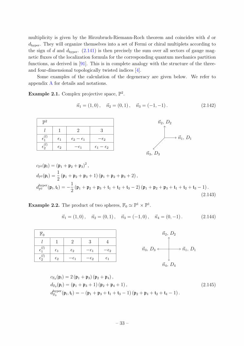
multiplicity is given by the Hirzubruch-Riemann-Roch theorem and coincides with d or
dhyper. They will organize themselves into a set of Fermi or chiral multiplets according to
the sign of d and dhyper. (2.141) is then precisely the sum over all sectors of gauge mag-
netic fluxes of the localization formula for the corresponding quantum mechanics partition
functions, as derived in [91]. This is in complete analogy with the structure of the three-
and four-dimensional topologically twisted indices [4].
Some examples of the calculation of the degeneracy are given below. We refer to
appendix A for details and notations.
Example 2.1. Complex projective space, P2.
~n1 = (1, 0) , ~n2 = (0, 1) , ~n3 = (−1,−1) . (2.142)
P2
l 1 2 3
ε(l)1 ε1 ε2 − ε1 −ε2ε
(l)2 ε2 −ε1 ε1 − ε2
~n1, D1
~n2, D2
~n3, D3
cP2(pl) = (p1 + p2 + p3)2 ,
dP2(pl) =1
2(p1 + p2 + p3 + 1) (p1 + p2 + p3 + 2) ,
dhyperP2 (pl, tl) = −1
2(p1 + p2 + p3 + t1 + t2 + t3 − 2) (p1 + p2 + p3 + t1 + t2 + t3 − 1) .
(2.143)
Example 2.2. The product of two spheres, F0 ' P1 × P1.
~n1 = (1, 0) , ~n2 = (0, 1) , ~n3 = (−1, 0) , ~n4 = (0,−1) . (2.144)
F0
l 1 2 3 4
ε(l)1 ε1 ε2 −ε1 −ε2ε
(l)2 ε2 −ε1 −ε2 ε1
~n1, D1
~n2, D2
~n3, D3
~n4, D4
cF0(pl) = 2 (p1 + p3) (p2 + p4) ,
dF0(pl) = (p1 + p3 + 1) (p2 + p4 + 1) ,
dhyperF0
(pl, tl) = − (p1 + p3 + t1 + t3 − 1) (p2 + p4 + t2 + t4 − 1) .
(2.145)
– 33 –
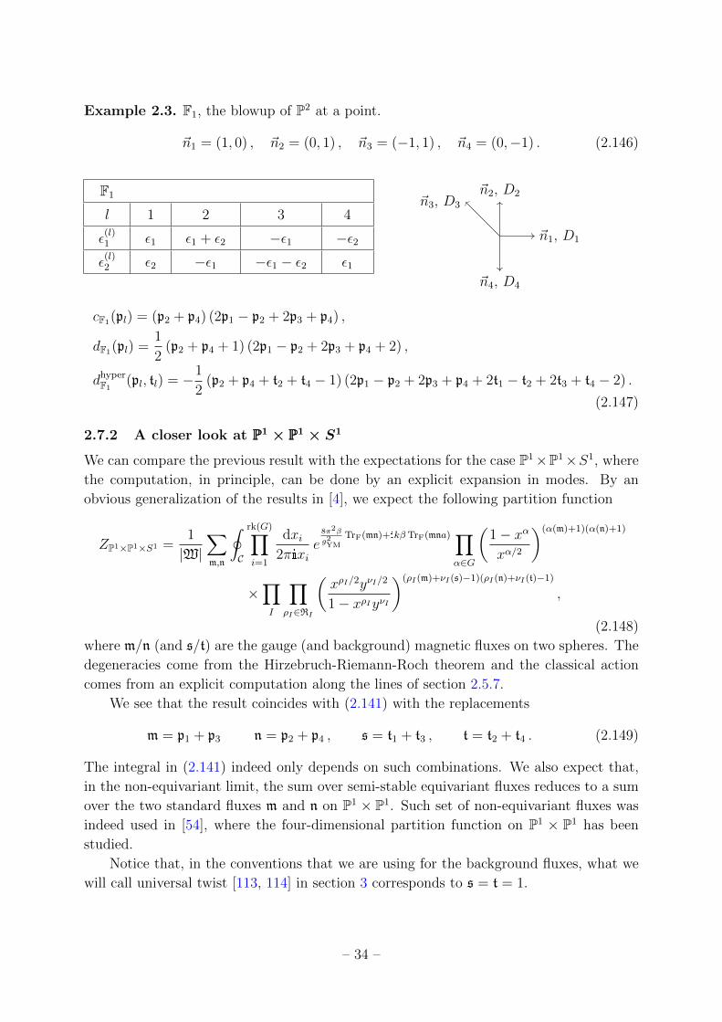
Example 2.3. F1, the blowup of P2 at a point.
~n1 = (1, 0) , ~n2 = (0, 1) , ~n3 = (−1, 1) , ~n4 = (0,−1) . (2.146)
F1
l 1 2 3 4
ε(l)1 ε1 ε1 + ε2 −ε1 −ε2ε
(l)2 ε2 −ε1 −ε1 − ε2 ε1
~n1, D1
~n2, D2~n3, D3
~n4, D4
cF1(pl) = (p2 + p4) (2p1 − p2 + 2p3 + p4) ,
dF1(pl) =1
2(p2 + p4 + 1) (2p1 − p2 + 2p3 + p4 + 2) ,
dhyperF1
(pl, tl) = −1
2(p2 + p4 + t2 + t4 − 1) (2p1 − p2 + 2p3 + p4 + 2t1 − t2 + 2t3 + t4 − 2) .
(2.147)
2.7.2 A closer look at PPP1 × PPP1 × S1
We can compare the previous result with the expectations for the case P1×P1×S1, where
the computation, in principle, can be done by an explicit expansion in modes. By an
obvious generalization of the results in [4], we expect the following partition function
ZP1×P1×S1 =1
|W|∑m,n
∮C
rk(G)∏i=1
dxi2πixi
e8π2β
g2YM
TrF(mn)+ikβTrF(mna) ∏α∈G
(1− xα
xα/2
)(α(m)+1)(α(n)+1)
×∏I
∏ρI∈RI
(xρI/2yνI/2
1− xρIyνI
)(ρI(m)+νI(s)−1)(ρI(n)+νI(t)−1)
,
(2.148)
where m/n (and s/t) are the gauge (and background) magnetic fluxes on two spheres. The
degeneracies come from the Hirzebruch-Riemann-Roch theorem and the classical action
comes from an explicit computation along the lines of section 2.5.7.
We see that the result coincides with (2.141) with the replacements
m = p1 + p3 n = p2 + p4 , s = t1 + t3 , t = t2 + t4 . (2.149)
The integral in (2.141) indeed only depends on such combinations. We also expect that,
in the non-equivariant limit, the sum over semi-stable equivariant fluxes reduces to a sum
over the two standard fluxes m and n on P1 × P1. Such set of non-equivariant fluxes was
indeed used in [54], where the four-dimensional partition function on P1 × P1 has been
studied.
Notice that, in the conventions that we are using for the background fluxes, what we
will call universal twist [113, 114] in section 3 corresponds to s = t = 1.
– 34 –
3 Large N limit
In this section, we analyze the large N limit of some of the topologically twisted indices
and other related quantities, finding an interesting structure.
In the large N limit we may expect some simplifications. In particular, instantons
are suppressed and the perturbative contribution to the topologically twisted index of 5D
N = 1 theories discussed in section 2 becomes exact. Moreover, we may also expect that
the choice of integration contour and the stability conditions on fluxes become simpler at
large N . In particular, we will work under the assumption that, in the large N limit, the
fluxes become actually independent.
In the topologically twisted index of 3D N = 2 theories on Σg1 × S1 [4, 8, 13, 18]
a distinguished role was played by the twisted superpotential W of the two-dimensional
theory obtained by compactification on S1 (with infinitely many KK modes). In partic-
ular, the partition function can be written as a sum over the set of Bethe vacua of the
two-dimensional theory, which corresponds to the critical points of W [8, 13]. Moreover,
in the large N limit, one particular Bethe vacuum dominates the partition function [5].
The natural quantity to consider for the 5D topologically twisted index is the SW pre-
potential F(a) of the four-dimensional theory obtained by compactification on S1. There
are two reasons to expect that the critical points of F(a) play a distinguished role in
five dimensions. First, the partition function of the topologically twisted N = 2 theories
in four dimensions can be split into two contributions, one coming from the integration
over the Coulomb plane (usually called the u plane), and the other from the locus where
monopoles and dyons become massless, corresponding to the critical points of the prepo-
tential F [115]. The integral over the u plane also often reduces to boundary contributions
from all the singular points in the moduli space. Secondly, in the integrable system ob-
tained by placing the four-dimensional theory on a Ω-background on R4 with ε1 = ~ and
ε2 = 0, the Bethe vacua read [116]
exp
(i∂W~(a)
∂aj
)= 1 , j = 1, . . . , rk(G) , (3.1)
where W~(a) is the twisted superpotential for the two-dimensional effective theory obtained
by reducing on the Ω-deformed copy of R2. We expect that these conditions play a role in
the equivariant partition function with ε1 = ~ and ε2 = 0. Since W~(a) has the following
expansion as ~→ 0,
W~(a) = −2π
~F(a) + . . . , (3.2)
we also obtain, in the limit ~→ 0, the quantization conditions (cf. [117, (3.62)] and [118,
(4.6)])
exp
(2πi
~aDj
)= exp
(2πi
~∂F(a)
∂aj
)= 1 , j = 1, . . . , rk(G) . (3.3)
It is possible that, in taking the non-equivariant limit of the index, the information about
the pole configurations of the integrand is partially lost and we need to impose extra
– 35 –
conditions following from (3.3). For all these reasons, we may think that the critical
points of F(a) may play a role in the evaluation of the index. In particular, in analogy
with the 3D index, we may expect that, in the large N limit, one particular critical point
of F(a) dominates the partition function. We will provide some evidence of this picture
by evaluating various quantities in the large N limit at the critical point of F(a) and
showing that they nicely agree with holographic predictions. Independently from these
considerations, the problem of finding the distribution of critical points of F(a) in the
large N limit is interesting in itself and deserves to be studied.
We will then consider the large N limit of the distribution of critical points of the
functional F(a) focusing on two 5D theories, N = 2 SYM, which decompactifies to the
N = (2, 0) theory in six dimensions and the N = 1 USp(2N) theory with Nf flavors and
an antisymmetric matter field, which corresponds to a 5D UV fixed point. In both cases we
find that the value of F(a) at its critical points, as a function of flavor fugacities, precisely
coincides, in the large N limit, with the partition function of the same theory on S5. This
is in parallel with what was found for the twisted superpotential of 3D N = 2 theories in
the large N limit [46], thus re-enforcing the analogy between the two quantities.
We shall then study the large N limit of the topologically twisted index of 5D N = 1
theories on P1×P1×S1. With no effort, we can replace P1×P1×S1 with the more general
manifold Σg2 ×Σg1 ×S1 and we will consider this more general case in the following. The
interest of this model is that we can formally dimensionally reduce on Σg2 and obtain
a three-dimensional theory. In three dimensions we can guess the form of the partition
function in the large N limit and use the results in [4, 8, 13, 18]. We expect the partition
function of the three-dimensional theory to be given as a sum over topological sectors
on Σg2 . We will denote the gauge/flavor magnetic fluxes on Σg1 and Σg2 by m/s and
n/t, respectively. We also denote by ∆ a complexified chemical potential for the flavor
symmetry. In each sector of gauge magnetic flux n on Σg2 we have a twisted superpotential
for the compactified theory satisfying [119]
∂W(a, n, ∆, t)
∂ni= −2π
∂F(a,∆)
∂ai,
∂W(a, n, ∆, t)
∂t= −2π
∂F(a,∆)
∂∆. (3.4)
One way to determine W is to compare the 5D partition function for P1×P1×S1 given in
section 2 with the structure of the topologically twisted index in three dimensions. This
is given by localization as a contour integral of a meromorphic quantity [4, 13, 18]∑m∈Γh
Z3Dint (a,m, n) =
∑m∈Γh
eimi
∂W(a,n)∂ai Z3D
int (a,m = 0, n) , (3.5)
where Γh is the lattice of gauge magnetic fluxes for the gauge group G. By generalizing
(2.148) from P1 × P1 to Σg1 ×Σg2 as in [18], and choosing a convenient parameterization
– 36 –
for the fluxes, we expect the integrand Z3Dint (a,m, n) to be(
detij
∂2W(a, n)
∂ai∂aj
)g1
e8π2β
g2YM
TrF(mn)+ikβTrF(mna) ∏α∈G
(1− xα
xα/2
)(α(m)+1−g1)(α(n)+1−g2)
×∏I
∏ρI∈RI
(xρI/2yνI/2
1− xρIyνI
)(ρI(m)+νI(s)+g1−1)(ρI(n)+νI(t)+g2−1)
.
(3.6)
We can therefore read off the twisted superpotential
Wpert(a, n,∆, t) = −8π2iβ
g2YM
TrF(na) +kβ
2TrF(na2)
+1
β
∑α∈G
(α(n) + 1− g2)
[Li2(xα)− 1
2g2 (−α(βa))
]− 1
β
∑I
∑ρI∈RI
(ρI(n) + νI(t) + g2 − 1)
[Li2(xρIyνI )− 1
2g2 (ρI(βa) + νI(β∆))
],
(3.7)
that indeed satisfies (3.4).
The topologically twisted index can then be computed as follows [8, 18]
ZpertΣg2×(Σg1×S1)(s, t, ∆) =
(−1)rk(G)
|W|∑n∈Γh
∑a=a(i)
Zpert∣∣m=0
(a, n)
(detij
∂2Wpert(a, n)
∂ai∂aj
)g1−1
,
(3.8)
where a(i) are the solutions to the Bethe ansatz equations (BAEs)
exp
(i∂Wpert(a, n;∆, t)
∂aj
)= 1 , j = 1, . . . , rk(G) . (3.9)
As we will see below, these BAEs (3.9) fix the value of the gauge magnetic fluxes ni in the
large N limit, hence, one needs an extra input in order to fix the value of the Coulomb
branch parameter ai. Assuming that the right condition to be imposed in the large N
limit is (3.3), we will be able to compute the index for both N = 2 SYM and the USp(2N)
theory.19 In particular, in the case of N = 2 SYM, thought of as compactification of the
6D N = (2, 0) theory on a circle, the index computes the elliptic genus of the 2D CFT
obtained by compactifying the 6D theory on Σg2 ×Σg1 . And, indeed, we find the correct
Cardy behaviour of the index in the high-temperature limit. This is in parallel with what
was found in [26] for the topologically twisted index of 4D N = 1 SCFTs on Σg1 × T 2.
Finally, we will also consider the large N limit of the twisted superpotential (3.7) and
the distribution of its critical points. We expect the on-shell value of Wpert to compute
some physical quantities of the intermediate compactification on Σg2 . We find indeed that
19An alternative method for evaluating the partition function of the USp(2N) theory is discussed in
appendix D.
– 37 –
this is the case. For N = 2 SYM, the critical value of Wpert is precisely the trial central
charge of the 4D SCFT obtained by compactifying the 6D (2, 0) theory on Σg2 , computed
both in field theory and holographically in [65, 66]. Quite remarkably, the identification
holds for an arbitrary assignment of R-charges for the trial central charge. For the USp(2N)
theory, the critical value of Wpert, extremized with respect to ∆, coincides with the S3 free
energy of the 3D theory, obtained by compactifying the 5D fixed point on Σg2 , recently
computed holographically in [64].20
3.1 N = 2 super Yang-Mills on Σg2 × (Σg1 × S1)
A decoupling limit of type IIB string theory on asymptotically locally Euclidean (ALE)
spaces predicts the existence of interacting 6D, N = (2, 0) theories labelled by an ADE
Lie algebra g = (An≥1, Dn≥4, E6, E7, E8) [120]. The AN−1 type can also be realized as the
low-energy description of the worldvolume theory of N coincident M5-branes in M-theory
[121]. A direct formulation of the (2, 0) theory has been a long standing problem. However,
it has been argued in [59–61] that the (2, 0) theory on a circle S1(6) of radius R6 is equivalent
to the five-dimensional N = 2 supersymmetric Yang-Mills (SYM) theory, whose coupling
constant is identified with the S1(6) radius by
R6 =g2
YM
8π2. (3.10)
We are interested in computing the partition function of the (2, 0) theory on Σg2 ×(Σg1×T 2), partially topologically twisted on Σg2×Σg1 . Given the above relation between
the (2, 0) theory and 5D maximally SYM, and considering the torus T 2 = S1×S1(6), this is
equivalent to compute the twisted partition function of N = 2 SYM on Σg2 × (Σg1 × S1).
A further reduction on S1 gives a four-dimensional theory. Recalling that the length of S1
is β, we see that the (complexified) gauge coupling of the four-dimensional theory can be
correctly identified with the modular parameter of the torus T 2 = S1 × S1(6),
τ =4πiβ
g2YM
=iβ
2πR6
. (3.11)
The twisted compactification of the (2, 0) theory onΣg1×Σg2 gives rise to anN = (0, 2)
SCFT in two dimensions [68]. The holonomy group of Σg1 × Σg2 is SO(2)1 × SO(2)2. In
order to preserve N = (0, 2) supersymmetry in two dimensions we turn on a background
Abelian gauge field coupled to an SO(2)2 subgroup of SO(5)R, embedded block-diagonally.
The right-moving trial central charge cr(∆) and the gravitational anomaly k = cr − cl for
this class of theories were computed in [68] and, at large N , they can be rewritten as (see
20The free energy on Σg2 × S3 as a function of ∆ was explicitly computed in field theory in [67] after
the completion of this work and perfectly agrees with the on-shell value of Wpert as a function of ∆.
– 38 –
also appendix C)
cr(s, t, ∆) ≈ cl(s, t, ∆) ≈ 2N3β2
(2π)2[∆1∆2(t1s2 + t2s1) + (∆1s2 +∆2s1)(∆1t2 +∆2t1)]
≈ N3β2
(2π)2
2∑ς,%=1
tςs%∂2(∆1∆2)2
∂∆ς∂∆%
,
(3.12)
where we introduced the democratic chemical potentials and fluxes for the SO(2)2 subgroup
of SO(5)R symmetry
∆1 = ∆ , ∆2 =2π
β−∆ ,
2∑ς=1
∆ς =2π
β,
s1 = s , s2 = 2(1− g1)− s ,2∑ς=1
sς = 2(1− g1) ,
t1 = t , t2 = 2(1− g2)− t ,2∑ς=1
tς = 2(1− g2) .
(3.13)
The partition function of the (2, 0) theory on Σg2× (Σg1×T 2) is just the elliptic genus
of the two-dimensional CFT. Thus we expect, in the high-temperature limit β → 0, where
β ≡ −2πiτ is a fictitious inverse temperature,21 the partition function to have a Cardy
behaviour
logZ(s, t, ∆) ≈ iπ
12τcr(s, t, ∆) . (3.14)
We will work in the ’t Hooft limit
N 1 with λ =g2
YMN
β= fixed , (3.15)
for which the instanton contributions to the partition function are exponentially sup-
pressed. The high-temperature limit of the partition function corresponds to large λ.
3.1.1 Effective prepotential at large N
The effective SW prepotential (2.136) of N = 2 SYM can be written as
F(a,∆) =N∑i=1
F cl(ai) +N∑i 6=j
F1-loop(ai − aj)−N∑
i,j=1
F1-loop(ai − aj +∆)
=2πiβ
g2YM
N∑i=1
a2i +
i
2πβ2
N∑i 6=j
Li3(eiβ(ai−aj))− i
2πβ2
N∑i,j=1
Li3(eiβ(ai−aj+∆))
− 1
4πβ2
N∑i 6=j
g3 (β(aj − ai)) +1
4πβ2
N∑i,j=1
g3 (β(ai − aj +∆)) .
(3.16)
21The torus partition function at a given τ corresponds to a thermal ensemble while the elliptic genus
is only counting extremal states. Therefore, the temperature represented by Im τ is fictitious.
– 39 –
The BAEs (3.3) are then given by
−8π2N
λai =
i
β
N∑j=1
[Li2(eiβ(ai−aj))− Li2(e−iβ(ai−aj))− Li2(eiβ(ai−aj+∆)) + Li2(e−iβ(ai−aj−∆))
]+
i
2β
N∑j=1
[−g2 (β(aj − ai)) + g2 (β(ai − aj))]
+i
2β
N∑j=1
[g2 (β(ai − aj +∆))− g2 (β(aj − ai +∆))] .
(3.17)
In the strong ’t Hooft coupling λ 1 the eigenvalues are pushed apart, i.e. | Im(ai−aj)| 1, and (3.17) can be approximated as
8π2N
λak ≈
i
2∆(2π − β∆)
N∑j=1
sign (Im(ak − aj)) . (3.18)
The sign function could be replaced by sign(i − j) if the eigenvalues ai are ordered by
increasing imaginary part. We thus find the solution
ak =iλ
16π2N[∆(2π − β∆)(2k −N − 1)] . (3.19)
It is also interesting to see what the value of the effective SW prepotential (3.16) at the
solution (3.19) is. In the strong ’t Hooft coupling λ 1 we find that
F(a,∆) ≈ 2πiN
λ
N∑i=1
a2i −
1
4πβ2
N∑i,j=1
[g3 (β(aj − ai)) + g3 (β(ai − aj +∆))] sign (Im(ai − aj))
=2πiN
λ
N∑i=1
a2i +
1
8π∆(2π − β∆)
N∑i,j=1
(ai − aj) sign (Im(ai − aj))
= −N∑j=1
[2πiN
λIm(aj)−
i
4π∆(2π − β∆)(2j −N − 1)
]Im(aj) .
(3.20)
In order to get the last equality we used the relation
N∑i,j=1
| Im(ai − aj)| = 2N∑j=1
(2j − 1−N) Im(aj) . (3.21)
Plugging the solution (3.19) back into (3.20), we obtain
F(∆) ≈ iβg2YMN
3
384π3(∆1∆2)2 . (3.22)
– 40 –
In order to obtain (3.22) we used
N∑k=1
(2k −N − 1)2 =1
3
(N3 −N
). (3.23)
Remarkably, the BAEs (3.18) and the SW prepotential in the large N limit (3.20),
(3.22) are identical to matrix model saddle point equations and free energy for the path
integral on S5 found in [122] (cf. [122, (4.13), (4.16) and (4.17)]).22
3.1.2 Effective twisted superpotential at large N
The effective twisted superpotential of the theory reads
W(a, n, ∆, t) = −8π2iβ
g2YM
N∑i=1
niai
+1
β
N∑i 6=j
(ni − nj + 1− g2)
[Li2(eiβ(ai−aj))− 1
2g2 (−β(ai − aj))
]
− 1
β
N∑i,j=1
(ni − nj + t + g2 − 1)
[Li2(eiβ(ai−aj+∆))− 1
2g2 (β(ai − aj +∆))
].
(3.24)
Let us try to find a solution to the BAEs (3.9). For the twisted superpotential (3.24), they
are given by23
8π2iβ
g2YM
ni1− g2
= i
N∑j(6=i)
[(ni − nj1− g2
+ 1
)Li1(eiβ(ai−aj))−
(nj − ni1− g2
+ 1
)Li1(e−iβ(ai−aj))
]
+1
2
N∑j(6=i)
[(ni − nj1− g2
+ 1
)g1 (−β(ai − aj))−
(nj − ni1− g2
+ 1
)g1 (β(ai − aj))
]
− i
N∑j=1
[(ni − nj + t
1− g2
− 1
)Li1(eiβ(ai−aj+∆))−
(nj − ni + t
1− g2
− 1
)Li1(e−iβ(ai−aj−∆))
]
+1
2
N∑j=1
[(ni − nj + t
1− g2
− 1
)g1 (β(ai − aj +∆))−
(nj − ni + t
1− g2
− 1
)g1 (−β(ai − aj −∆))
].
(3.25)
In the strong ’t Hooft coupling limit, i.e. λ 1, (3.25) can be approximated as
ni ≈iλβ
16π2N(∆1t2 +∆2t1)
N∑j(6=i)
sign (Im(ai − aj)) . (3.26)
22One needs to set ∆1 = π(1 + 2i
3 mthere
)and ∆2 = π
(1− 2i
3 mthere
).
23The BAEs actually read ∂Wpert
∂aj= 2πlj where lj ∈ Z are angular ambiguities. Since lj ’s are generically
of order one they are negligible in the final solution and we set them to zero in the following.
– 41 –
The sign function in (3.26) could be replaced by sign(i−j) if the eigenvalues ai are ordered
by increasing imaginary part. We thus find that
nk ≈iλβ
16π2N(∆1t2 +∆2t1)(2k −N − 1) . (3.27)
Note that the above result is neither real nor integer. This is peculiar to the limit λ 1.
Since the nk’s are large we treat them effectively as a continuous variable. We also consider
the above result as a complex saddle point contribution to the partition function.
The twisted superpotential (3.24) at strong ’t Hooft coupling limit can be approxi-
mated as
W(a, n, ∆, t)
1− g2
≈ − 8π2iN
λ(1− g2)
N∑i=1
niai
− 1
2β
N∑i,j=1
(ni − nj1− g2
+ 1
)g2 (−β(ai − aj)) sign (Im(ai − aj))
+1
2β
N∑i,j=1
(ni − nj + t
1− g2
− 1
)g2 (β(ai − aj +∆)) sign (Im(ai − aj)) .
(3.28)
This can be further simplified to
W(a, n, ∆, t) ≈ 8π2N
λ
N∑j=1
Im(aj)
[nj −
iλβ
16π2N(∆1t2 +∆2t1)(2j −N − 1)
]
− β
4∆1∆2
N∑i,j=1
(ni − nj) sign (Im(ai − aj)) .
(3.29)
Plugging (3.27) back into (3.29), all the dependence on ai goes away and we are left with
W(∆, t) ≈ −β4∆1∆2
N∑i,j=1
(ni − nj) sign (Im(ai − aj))
= −iβg2YMN
3
96π2∆1∆2(∆1t2 +∆2t1) .
(3.30)
This can be more elegantly rewritten as
W(∆, t) ≈ −2π2∑ς=1
tς∂F(∆)
∂∆ς
, (3.31)
where F(∆) is given in (3.22).
– 42 –
W(∆, t) and the 4D central charge. Remarkably, we find the following relation
between the twisted superpotential (3.30) and the conformal anomaly coefficient a(∆, t) of
the four-dimensional N = 1 theory that is obtained by compactifying the 6D N = (2, 0)
theory on Σg2 [65, 66],
W(∆, t) ≈ − 8π2
27βτa(∆, t) , (3.32)
where τ is the four-dimensional coupling constant.
Indeed, the central charge of the 4D theory, at large N , can be written as
a(∆, t) ≈ −9N3
128
2∑ς=1
tς∂(∆1∆2)2
∂∆ς
, (3.33)
where we used ∆ς = β∆ς/π, satisfying ∆1 + ∆2 = 2, to parameterize a trial R-symmetry
of the 4D N = 1 theory. (3.33) can be easily derived from the results in [65, 66] (cf. for
example [66, (2.22)]). It can be also more straightforwardly derived as in appendix C.
Curiously, the same relation between the twisted superpotential and the central charge
in (3.32) was found for a class ofN = 1 gauge theories on S2×T 2, with a partial topological
twist along S2 [26].
3.1.3 Partition function at large N
The topologically twisted index of 5D N = 2 SYM on Σg2 × (Σg1 × S1) reads
Z(y, s, t) =1
N !
∑m,n∈ZN
∮C
N∏i=1
dxi2πixi
e8π2β
g2YM
(mi−mj)(ni−nj)(
detij
∂2W(a, n)
∂ai∂aj
)g1
×N∏i 6=j
(1− xi/xj√
xi/xj
)(mi−mj+1−g1)(ni−nj+1−g2)
×N∏
i,j=1
( √xiy/xj
1− xiy/xj
)(mi−mj+s+g1−1)(ni−nj+t+g2−1)
.
(3.34)
This can be evaluated using (3.8). We can write
Z(y, s, t) =(−1)N
N !
( √y
1− y
)N(g1+s−1)(g2+t−1) ∑n∈ZN
∑a=a(i)
(detij
∂2W(a, n)
∂ai∂aj
)g1−1
×N∏i 6=j
(1− xi/xj√
xi/xj
)(1−g1)(ni−nj+1−g2)( √xiy/xj
1− xiy/xj
)(s+g1−1)(ni−nj+t+g2−1)
.
(3.35)
– 43 –
We are interested in the logarithm of the partition function in the strong ’t Hooft coupling
limit. The only piece which survives in this limit is given by
logZ(1) ≡ logN∏i 6=j
(1− xi/xj√
xi/xj
)(1−g1)(ni−nj+1−g2)( √xiy/xj
1− xiy/xj
)(s+g1−1)(ni−nj+t+g2−1)
= −N∑i 6=j
(1− g1)(ni − nj + 1− g2)
[Li1(eiβ(ai−aj))− i
2g1 (−β(ai − aj))
]
+N∑i 6=j
(s + g1 − 1)(ni − nj + t + g2 − 1)
[Li1(eiβ(ai−aj+∆)) +
i
2g1 (β(ai − aj +∆))
].
(3.36)
In the strong ’t Hooft coupling limit it can be approximated as
logZ(1) ≈ −iβ
4
N∑i 6=j
[(ai − aj)(t1s2 + t2s1) + (ni − nj)(∆1s2 +∆2s1)] sign (Im(ai − aj))
=β
2
N∑j=1
(2j − 1−N) [(t1s2 + t2s1) Im(aj)− i(∆1s2 +∆2s1)nj] ,
(3.37)
where we assumed that the eigenvalues ai are ordered by increasing imaginary part, and
used the relationN∑
i,j=1
(ni − nj) sign(i− j) = 2N∑j=1
(2j −N − 1)ni . (3.38)
Plugging the solutions (3.19) and (3.27) back into (3.37), we find that
logZ ≈ βg2YMN
3
96π2[∆1∆2(t1s2 + t2s1) + (∆1s2 +∆2s1)(∆1t2 +∆2t1)]
= i
2∑ς=1
sς∂W(t, ∆)
∂∆ς
= −2iπ2∑
ς,%=1
sςt%∂2F(∆)
∂∆ς∂∆%
=g2
YMN3
192π2β
2∑ς,%=1
sςt%∂2(β∆1∆2)2
∂∆ς∂∆%
,
(3.39)
where W(t, ∆) is given in (3.30) and we used (3.31) in writing the last equality. (3.39) can
be also expressed in terms of the trial right-moving central charge of the 2D N = (0, 2)
SCFT, see (3.12), as
logZ(s, t, ∆) ≈ iπ
12τcr(s, t, ∆) ≈ − 8iπ2
27βτ
2∑ς=1
sς∂a(t, ∆)
∂∆ς
. (3.40)
In writing the second equality we used the relation (3.32). In [26], the very same Cardy
behaviour (3.40) of the partition function in the high-temperature limit has been proved
for a class of N = 1 gauge theories on S2 × T 2, with a partial topological twist along S2.
– 44 –
3.1.4 Counting states and the I-extremization principle
The topologically twisted index of the 6D (2, 0) theory on Σg2×Σg1×T 2 can be interpreted
as a trace over a Hilbert space of states on Σg2 ×Σg1 × S1:
Z(s, t, ∆) = TrΣg2×Σg1×S1(−1)F qHLyJ , (3.41)
where q = e2πiτ , y = eiβ∆ and the Hamiltonian HL on Σg2×Σg1×S1 explicitly depends on
the magnetic fluxes sς , tς (ς = 1, 2). The number of supersymmetric ground states dmicro
with momentum n and electric charge q under the Cartan subgroup of the flavor symmetry
commuting with the Hamiltonian – in the microcanonical ensemble – is then given by the
Fourier transform of (3.41) with respect to (τ,∆):
dmicro(s, t, n, q) = − iβ
(2π)2
∫iR
dβ
∫ 2πβ
0
d∆Z(s, t, ∆) eβn−iβ∆q , (3.42)
where β = −2πiτ and the corresponding integration is over the imaginary axis.
In the limit of large charges, we may use the saddle point approximation. Consider for
simplicity q = 0. The number of supersymmetric ground states dmicro with charges (s, t, n)
can be obtained by extremizing
ISCFT(β, ∆) ≡ logZ(s, t, ∆) + βn =N3
24β
2∑ς,%=1
sςt%∂2(β∆1∆2)2
∂∆ς∂∆%
+ nβ , (3.43)
with respect to ∆ and β, i.e.
∂I(β, ∆)
∂∆= 0 ,
∂I(β, ∆)
∂β= 0 , (3.44)
and evaluating it at its extremum
log dmicro(s, t, n, 0) = I∣∣crit
(s, t, n) . (3.45)
Given (3.40), we see that the extremization with respect to ∆ is the c-extremization
principle [45, 68] and sets the trial right-moving central charge cr(s, t, ∆) to its exact value
cCFT ≈ cr ≈ cl in the IR. For the case at our disposal, (3.12) has a critical point at
∆ = −2π
β
t1s2 + t2s1 − t1s1
s1(t1 − 2t2) + s2(t2 − 2t1), (3.46)
and its value at ∆ reads
cCFT(s, t) ≈ −2N3 t21s22 + t1t2s1s2 + t22s
21
s1(t1 − 2t2) + s2(t2 − 2t1). (3.47)
Extremizing I(β, ∆) with respect to β yields
¯β(s, t, n) = π
√cCFT(s, t)
6n. (3.48)
– 45 –
Plugging back (3.46) and (3.48) into I(β, ∆), we find that
ISCFT
∣∣crit
(s, t, n) = 2π
√n cCFT(s, t)
6. (3.49)
This is obviously nothing else than Cardy formula [123].
This procedure corresponds to the I-extremization principle used for BPS black holes
(strings) [5, 24, 26, 27] in the context of the AdS4(5) /CFT3(4) correspondence and contains
two basic pieces of information:
1. extremizing the index unambiguously determines the exact R-symmetry of the SCFT
in the IR;
2. the value of the index at its extremum is the (possibly regularized) number of ground
states.
We will apply this counting to supergravity black strings and black holes in section 4.
3.2 USp(2N) theory with matter on Σg2 × (Σg1 × S1)
In this section we focus on gauge theories with a conjectured massive type IIA dual [124]
(see also [57, 58, 125, 126]) and compute their partition function at large N . The dual
supergravity backgrounds have a warped AdS6 × S4 geometry. The stringy root of this
theories is in type I’ string theory as strongly coupled microscopic theories on the intersec-
tion of N D4-branes and Nf D8-branes and orientifold planes. The worldvolume theory
on the N D4-branes plus their images is a USp(2N) gauge theory with Nf hypermulti-
plets in the fundamental representation and one hypermultiplet A in the antisymmetric
representation of USp(2N). In addition to the SU(2) R-symmetry the theory has an
SU(2)M ×SO(2Nf )×U(1)I global symmetry: SU(2)M acts on A as a doublet, SO(2Nf ) is
the flavor symmetry associated to the fundamental hypermultiplets, and U(1)I is the topo-
logical symmetry associated to the conserved instanton number current j = ∗Tr(F∧F ). At
the fixed point, the SO(2Nf )×U(1)I part of the symmetry is enhanced non-perturbatively
to an exceptional group ENf+1, due to the instanton which becomes massless at the origin
of the Coulomb branch of the fixed point theory [57]. Finally, in the large N limit the free
energy of the USp(2N) theory on S5 reads [127]
FS5 ≈ −9√
2πN5/2
5√
8−Nf
. (3.50)
The Cartan of USp(2N) has N elements which we denote by ui, i = 1, . . . , N . We
normalize the weights of the fundamental representation of USp(2N) to be ±ei (so they
form a basis of unit vectors for RN). The antisymmetric representation thus has weights
±ei ± ej with i > j and N − 1 zero weights, and the roots are ±ei ± ej with i > j and
±2ei. As we shall see below, at large N , ui = O(N1/2) (see (3.52) with α = 1/2). Hence,
the contributions with nontrivial instanton numbers are exponentially suppressed in the
large N limit.
We set the length of S1 to one, i.e. β = 1, throughout this section.
– 46 –
3.2.1 Effective prepotential at large N
The effective prepotential of the theory is then given by (2.136):
F(ai, ∆K) =N∑i=1
Fpert(±2ai)−Nf∑f=1
Fpert(±ai +∆f )
+
N∑i>j
[Fpert(±ai ± aj)−Fpert(±ai ± aj +∆m)
]+ (N − 1)Fpert(∆m) ,
(3.51)
where the index K labels all the matter fields in the theory. Here, we introduced the
notation F(±a) ≡ F(a)+F(−a). Notice that the contribution of the last term to the large
N prepotential is of O(N2) and thus subleading. Let us analyze the effective prepotential
(3.51) assuming that the eigenvalues grow in the large N limit. We restrict to Im ai > 0
due to the Weyl reflections of the USp(2N) group. We consider the following large N
saddle point eigenvalue distribution ansatz:
aj = iNαtj , (3.52)
for some number 0 < α < 1 to be determined later. At large N , we define the continuous
function tj = t(j/N) and we introduce the density of eigenvalues
ρ(t) =1
N
dj
dt, (3.53)
normalized so that∫
dtρ(t) = 1. In the large N limit the sums over N become Riemann
integrals, for example,N∑j=1
→ N
∫dtρ(t) . (3.54)
Consider the first line in (3.51):
i
2π
N∑i=1
[Li3(e2iai) + Li3(e−2iai)−
Nf∑f=1
Li3(ei(ai+∆f ))−Nf∑f=1
Li3(e−i(ai−∆f ))
]
− 1
4π
N∑i=1
[g3(−2ai) + g3(2ai) +
Nf∑f=1
g3(ai +∆f ) +
Nf∑f=1
g3(−ai +∆f )
].
(3.55)
The second line is of O(N2α+1) and thus subleading in the large N limit (as we see below).
Using the ansatz (3.52) we may write
F (0) ≈iN
2π
∫dtρ(t)
[Li3(e−2Nαt) + Li3(e2Nαt)−
Nf∑f=1
Li3(e−Nαt+i∆f )−
Nf∑f=1
Li3(eNαt+i∆f )
]≈ −i(8−Nf )
12πN1+3α
∫dtρ(t)t3 [Θ(t)−Θ(−t)] +O(N2α+1)
= −i(8−Nf )
12πN1+3α
∫dtρ(t)|t|3 +O(N2α+1) ,
(3.56)
– 47 –
where Θ(t) is the Heaviside theta function. Now, let us focus on the second line of (3.51).
Consider the following terms
F (1)hyper = − i
2π
N∑i>j
[Li3(ei(ai−aj+∆m)) + Li3(e−i(ai−aj−∆m))
]− 1
4π
N∑i>j
[g3(ai − aj +∆m) + g3(aj − ai +∆m)] .
(3.57)
At large N , we obtain
F (1)hyper ≈ −
iN2
4π
∫dtρ(t)
∫dt′ρ(t′)
[Li3(e−N
α(t−t′)+i∆m) + Li3(eNα(t−t′)+i∆m)
]− N2
8π
∫dtρ(t)
∫dt′ρ(t′)
[(π −∆m)N2α(t− t′)2 + 2g3(∆m)
]≈ N2
4π
∫dtρ(t)
∫dt′ρ(t′)g3 (−iNα(t′ − t) +∆m)Θ(t′ − t)
+N2
4π
∫dtρ(t)
∫dt′ρ(t′)g3 (−iNα(t− t′) +∆m)Θ(t− t′)
− N2
8π
∫dtρ(t)
∫dt′ρ(t′)
[(π −∆m)N2α(t− t′)2 + 2g3(∆m)
]=
iN2
4π
∫dtρ(t)
∫dt′ρ(t′)
(1
6N3α |t− t′|3 − g2(∆m)Nα |t− t′|
).
(3.58)
Next, consider
F (1)vector =
i
2π
N∑i>j
[Li3(ei(ai−aj)) + Li3(e−i(ai−aj)) +
i
2g3(aj − ai) +
i
2g3(ai − aj)
]. (3.59)
Its contribution can be simply obtained by, see (E.5),
F (1)vector = −F (1)
hyper
∣∣∆m=2π
. (3.60)
We thus find
F (1)vector + F (1)
hyper ≈i
4π
[π2
3− g2(∆m)
]N2+α
∫dtρ(t)
∫dt′ρ(t′) |t− t′| . (3.61)
The next term that we shall consider is the following
F (2)hyper = − i
2π
N∑i>j
[Li3(ei(ai+aj+∆m)) + Li3(e−i(ai+aj−∆m))
]− 1
4π
N∑i>j
[g3(ai + aj +∆m) + g3(−ai − aj +∆m)] .
(3.62)
– 48 –
The first term in the first line is exponentially suppressed in the large N limit (since
Im ai > 0 ,∀i). We then get
F (2)hyper ≈ −
iN2
4π
∫dtρ(t)
∫dt′ρ(t′) Li3(eN
α(t+t′)+i∆m)
− N2
8π
∫dtρ(t)
∫dt′ρ(t′)
[(π −∆m)N2α(t+ t′)2 + 2g3(∆m)
]≈ N2
4π
∫dtρ(t)
∫dt′ρ(t′)g3(−iNα(t+ t′) +∆m)
− N2
8π
∫dtρ(t)
∫dt′ρ(t′)
[(π −∆m)N2α(t+ t′)2 + 2g3(∆m)
]=
iN2
4π
∫dtρ(t)
∫dt′ρ(t′)
[1
6N3α(t+ t′)3 − g2(∆m)Nα(t+ t′)2
].
(3.63)
The last term that we shall consider reads
F (2)vector =
i
2π
N∑i>j
[Li3(ei(ai+aj)) + Li3(e−i(ai+aj)) +
i
2g3(−ai − aj) +
i
2g3(ai + aj)
]. (3.64)
Its contribution can be simply obtained by, see (E.5),
F (2)vector = −F (2)
hyper
∣∣∆m=2π
. (3.65)
We thus find that
F (2)vector + F (2)
hyper ≈i
4π
[π2
3− g2(∆m)
]N2+α
∫dtρ(t)
∫dt′ρ(t′)(t+ t′) . (3.66)
Putting (3.56), (3.61), and (3.66) together we obtain the final expression for the effective
prepotential at large N :
F [ρ(t), ∆m] = F (0) +2∑
ϑ=1
(F (ϑ)
vector + F (ϑ)hyper
)≈ −i(8−Nf )
12πN1+3α
∫ t∗
0
dtρ(t)|t|3 − µ(∫ t∗
0
dtρ(t)− 1
)+
i
4π
[π2
3− g2(∆m)
]N2+α
∫ t∗
0
dtρ(t)
∫ t∗
0
dt′ρ(t′) [|t− t′|+ (t+ t′)] ,
(3.67)
where we added the Lagrange multiplier µ for the normalization of ρ(t). α will be de-
termined to be 1/2 by the competition between the first and the last term in (3.67), and
therefore F ∝ N5/2. Remarkably, the effective prepotential (3.67) equals the large N
expression of the S5 free energy computed in [127, (3.4)] (see also [128, (3.14)]). This
is in complete analogy with the observation made in [46]. There, the effective twisted
superpotential of a three-dimensional N = 2 theory on A-twisted Σg1 × S1 was shown to
be equal to the S3 free energy of the same N = 2 theory, both evaluated at large N .
– 49 –
Extremizing (3.67) with respect to the continuous function ρ(t) we find the following
saddle point equation
2iπµ
N5/2=
(8−Nf )
6|t′|3 −
[π2
3− g2(∆m)
] ∫ t∗
0
ρ(t) [|t− t′|+ (t+ t′)] . (3.68)
On the support of ρ(t) the solution reads
ρ(t) =2|t|t2∗
, t∗ =2√
8−Nf
[π2
3− g2(∆m)
]1/2
,
µ =4i
3π
N5/2√8−Nf
[π2
3− g2(∆m)
]3/2
.
(3.69)
Evaluating (3.67) at (3.69) yields24
F(∆m) ≈ 23/2i
15π
N5/2√8−Nf
[∆m(2π −∆m)]3/2 . (3.70)
Finally, let us rewrite (3.70) as
F(∆) ≈ 23/2i
15π
N5/2√8−Nf
(∆1∆2)3/2 , (3.71)
for later use. Here we introduced the democratic chemical potentials
∆1 = ∆m , ∆2 = 2π −∆m . (3.72)
3.2.2 Effective twisted superpotential at large N
We are interested in the large N limit of the effective twisted superpotential
Wpert(a, n, ∆, t) =N∑i=1
[Wpert(±2ai)−
Nf∑f=1
Wpert(±ai +∆f )
]
+N∑i>j
[Wpert(±ai ± aj)− Wpert(±ai ± aj +∆m)
]+ (N − 1)Wpert(∆m) .
(3.73)
We consider the following ansatz for the large N saddle point eigenvalue distribution
ai = iNαti , ni = iNαNi . (3.74)
24F(∆m) = 25µ(∆m) due to a virial theorem for the large N prepotential (3.67).
– 50 –
Consider the first line in (3.73):
W(0) =N∑i=1
(±2ni + 1− g2)
[Li2(e±2iai)− 1
2g2(∓2ai)
]
−Nf∑f=1
N∑i=1
(ni + tf + g2 − 1)
[Li2(ei(ai+∆f ))− 1
2g2(ai +∆f )
]
−Nf∑f=1
N∑i=1
(−ni + tf + g2 − 1)
[Li2(e−i(ai−∆f ))− 1
2g2(−ai + ∆f )
].
(3.75)
The g2 terms are of O(N2) and thus subleading in the large N limit. Hence,
W(0) ≈ i(8−Nf )
2N1+3α
∫dtρ(t)N(t)t2 sign(t) . (3.76)
Now, let us focus on the second line of (3.73). Consider the following terms
W(1)hyper = −
N∑i>j
(ni − nj + tm + g2 − 1)
[Li2(ei(ai−aj+∆m))− 1
2g2(ai − aj +∆m)
]
−N∑i>j
(nj − ni + tm + g2 − 1)
[Li2(e−i(ai−aj−∆m))− 1
2g2(aj − ai +∆m)
].
(3.77)
At large N , we obtain
W(1)hyper ≈ −
i
4N2+3α
∫dtρ(t)
∫dt′ρ(t′)(N(t)−N(t′))(t− t′)2 sign(t− t′)
+i
4g2(∆1)N2+α
∫dtρ(t)
∫dt′ρ(t′)(N(t)−N(t′)) sign(t− t′)
+i
8(∆1 −∆2)(t1 − t2)N2+α
∫dtρ(t)
∫dt′ρ(t′)|t− t′| ,
(3.78)
where we used the democratic chemical potentials and fluxes
∆1 = ∆m , ∆2 = 2π −∆m , t1 = tm , t2 = 2(1− g2)− tm . (3.79)
The similar contribution coming from the vector multiplet can be obtained by using
Wpertvector = −Wpert
hyper|tm=2(1−g2),∆m=2π . (3.80)
It reads
W(1)vector ≈
i
4N2+3α
∫dtρ(t)
∫dt′ρ(t′)(N(t)−N(t′))(t− t′)2 sign(t− t′)
− iπ2
6N2+α
∫dtρ(t)
∫dt′ρ(t′)(N(t)−N(t′)) sign(t− t′)
− iπ
2(1− g2)N2+α
∫dtρ(t)
∫dt′ρ(t′)|t− t′| .
(3.81)
– 51 –
We thus find that
W(1)vector + W(1)
hyper ≈ −i
4∆1∆2N
2+α
∫dtρ(t)
∫dt′ρ(t′)(N(t)−N(t′)) sign(t− t′)
− i
4(∆1t2 +∆2t1)N2+α
∫dtρ(t)
∫dt′ρ(t′)|t− t′| .
(3.82)
The next term we shall consider is given by
W(2)vector + W(2)
hyper =N∑i>j
(ni + nj + 1− g2)
[Li2(ei(ai+aj))− 1
2g2(−ai − aj)
]
+N∑i>j
(−ni − nj + 1− g2)
[Li2(e−i(ai+aj))− 1
2g2(ai + aj)
]
−N∑i>j
(ni + nj + tm + g2 − 1)
[Li2(ei(ai+aj+∆m))− 1
2g2(ai + aj +∆m)
]
−N∑i>j
(−ni − nj + tm + g2 − 1)
[Li2(e−i(ai+aj−∆m))− 1
2g2(−ai − aj +∆m)
].
(3.83)
In the large N limit it can be approximated as
W(2)vector + W(2)
hyper ≈ −i
4∆1∆2N
2+α
∫dtρ(t)
∫dt′ρ(t′)(N(t) + N(t′))
− i
4(∆1t2 +∆2t1)N2+α
∫dtρ(t)
∫dt′ρ(t′)(t+ t′) .
(3.84)
Putting (3.76), (3.82), and (3.84) together we obtain the final expression for the effective
twisted superpotential at large N :
W [ρ(t),N(t), ∆m, tm] = W(0) +2∑
ϑ=1
(W(ϑ)
vector + W(ϑ)hyper
)≈ i
(8−Nf )
2N1+3α
∫ t∗
0
dtρ(t)N(t)t2 − iγ
(∫ t∗
0
dtρ(t)− 1
)− i
4(∆1∆2)N2+α
∫ t∗
0
dtρ(t)
∫ t∗
0
dt′ρ(t′)(N(t)−N(t′)) sign(t− t′)
− i
4(∆1∆2)N2+α
∫ t∗
0
dtρ(t)
∫ t∗
0
dt′ρ(t′)(N(t) + N(t′))
− i
4(∆1t2 +∆2t1)N2+α
∫ t∗
0
dtρ(t)
∫ t∗
0
dt′ρ(t′) [|t− t′|+ (t+ t′)] ,
(3.85)
where we added the Lagrange multiplier γ for the normalization of ρ(t). In order to have
a non-trivial saddle point we need to set 1 + 3α = 2 + α, implying that α = 1/2. The
– 52 –
twisted superpotential thus scales as N5/2. Setting to zero the variation with respect to
ρ(t), we get the equation
γ
N5/2=
(8−Nf )
2N(t′)t′2 − 1
2(∆1t2 +∆2t1)
∫ t∗
0
ρ(t) [|t+ t′|+ (t+ t′)]
− 1
2(∆1∆2)
∫ t∗
0
[(N(t)−N(t′)) sign(t− t′) + (N(t) + N(t′))] .
(3.86)
On the support of ρ(t) the solution is given by
ρ(t) =2|t|t2∗
, t∗ =(2∆1∆2)1/2√
8−Nf
, N(t) =1
2
(t1∆1
+t2∆2
)t ,
γ = − N5/2√8−Nf
(2∆1∆2)1/2(∆1t2 +∆2t1) .
(3.87)
Evaluating (3.85) at (3.87) yields25
W(∆m, tm) ≈ − 23/2iN5/2
5√
8−Nf
(∆1∆2)1/2(∆1t2 +∆2t1) . (3.88)
This can be more elegantly rewritten as
W(∆m, tm) ≈ −2π2∑ς=1
tς∂F(∆)
∂∆ς
, (3.89)
where F(∆) is given in (3.71).
W and the free energy on Σg2 × S3. Remarkably, we find the following relation
between the twisted superpotential (3.89) and the S3 free energy of the 3D N = 2 theory
that is obtained by compactifying the 5D theory on Σg2 with fluxes tς :
W(∆m, t) ≈iπ
2FΣg2×S3(t) , (3.90)
where W(∆m, t) is evaluated at its extremum
∆m
π=
5t1 − 3t2 ±√
9t21 − 14t1t2 + 9t224(t1 − t2)
. (3.91)
Indeed, the S3 free energy was very recently computed holographically in [64] and it
reads
FΣg2×S3(t) ≈ 16π
5
(1− g2)N5/2
κ√
8−Nf
(z2 − κ2)3/2(√
κ2 + 8z2 − κ)(
4z2 − κ2 + κ√κ2 + 8z2
)3/2, (3.92)
25W(∆m, tm) = 2i5 γ(∆m, tm) due to a virial theorem for the large N twisted superpotential (3.85).
– 53 –

where κ = 1 for g2 = 0 and κ = −1 for g2 > 1 and the variable z parameterizes the fluxes
tς . In the special case of the torus, g2 = 1, the above expression should be replaced by
FΣg2×S3(t) ≈ 4√
2π
5
N5/2√8−Nf
|z| . (3.93)
It is now a simple exercise to check that (3.90) holds identically for all g2 upon iden-
tifying
t1 = (1− g2)(
1 +z
κ
), t2 = (1− g2)
(1− z
κ
). (3.94)
We expect that (3.90) holds also off-shell
W(∆, t) ≈ iπ
2FΣg2×S3(∆, t) , (3.95)
where FΣg2×S3(∆, t) is the free energy as a function of a trial R-symmetry. (3.90) would
correspond then to the statement that the S3 free energy of the 3D theory is obtained by
extremizing FΣg2×S3(∆, t) with respect to ∆ [129].26
3.2.3 Partition function at large N
The topologically twisted index of the USp(2N) theory with matter on Σg2 × (Σg1 × S1)
reads
Zpert(y, s, t) =(−1)N
2NN !
∑n∈Γh
∑a=a(i)
(detij
∂2W(a, n)
∂ai∂aj
)g1−1
×(
y1/2m
1− ym
)(N−1)(sm+g1−1)(tm+g2−1) ∏g=±1
N∏i=1
(1− x2g
i
xgi
)(1−g1)(2gni+1−g2)
×N∏i=1
Nf∏f=1
(x
1/2i y
1/2f
1− xiyf
)(sf+g1−1)(ni+tf+g2−1)( x−1/2i y
1/2f
1− x−1i yf
)(sf+g1−1)(−ni+tf+g2−1)
×∏g=±1
N∏i>j
(1− (xixj)
g
(xixj)g/2
)(1−g1)(gni+gnj+1−g2)(1− (xi/xj)
g
(xi/xj)g/2
)(1−g1)(gni−gnj+1−g2)
×∏g=±1
N∏i>j
((xixj)
g/2y1/2m
1− (xixj)gym
)(sm+g1−1)(gni+gnj+tm+g2−1)
×∏g=±1
N∏i>j
((xi/xj)
g/2y1/2m
1− (xi/xj)gym
)(sm+g1−1)(gni−gnj+tm+g2−1)
.
(3.96)
26The free energy on Σg2 × S3 as a function of ∆ was explicitly computed in field theory in [67] after
the completion of this work. The result in [67] perfectly agrees with (3.95).
– 54 –
The products∏N
i=1 are of O(N2) and thus subleading in the large N limit. Then we
consider the last line in (3.96):
logZ(1)hyper = (sm + g1 − 1)
N∑i>j
(ni − nj + tm + g2 − 1)
[Li1(ei(ai−aj+∆m)) +
i
2g1(ai − aj +∆m)
]
+ (sm + g1 − 1)N∑i>j
(nj − ni + tm + g2 − 1)
[Li1(e−i(ai−aj−∆m)) +
i
2g1(aj − ai +∆m)
].
(3.97)
At large N , it can be approximated as
logZ(1)hyper ≈ −
1
8(∆1 −∆2)(s1 − s2)N2+α
∫dtρ(t)
∫dt′ρ(t′)(N(t)−N(t′)) sign(t− t′)
− 1
8(t1 − t2)(s1 − s2)N2+α
∫dtρ(t)
∫dt′ρ(t′)|t− t′| ,
(3.98)
where we introduced the democratic fluxes
s1 = sm , s2 = 2(1− g1)− sm . (3.99)
The similar contribution coming from the vector multiplet can be obtained by using
logZpertvector = − logZpert
hyper|sm=2(1−g1), tm=2(1−g2),∆m=2π . (3.100)
It reads
logZ(1)vector ≈
π
2(1− g1)N2+α
∫dtρ(t)
∫dt′ρ(t′)(N(t)−N(t′)) sign(t− t′)
+1
2(1− g2)(1− g1)N2+α
∫dtρ(t)
∫dt′ρ(t′)|t− t′| .
(3.101)
We thus find that
logZ(1)vector + logZ
(1)hyper ≈
1
4(∆1s2 +∆2s1)N2+α
∫dtρ(t)
∫dt′ρ(t′)(N(t)−N(t′)) sign(t− t′)
+1
4(t1s2 + t2s1)N2+α
∫dtρ(t)
∫dt′ρ(t′)|t− t′| .
(3.102)
The terms coming from the roots e1 + e2 and −e1 − e2 are treated as in (3.98). They can
be approximated at large N as
logZ(2)vector + logZ
(2)hyper ≈
1
4(∆1s2 +∆2s1)N2+α
∫dtρ(t)
∫dt′ρ(t′)(N(t) + N(t′))
+1
4(t1s2 + t2s1)N2+α
∫dtρ(t)
∫dt′ρ(t′)(t+ t′) .
(3.103)
– 55 –
Putting everything together we obtain the following functional for the logarithm of the
partition function at large N :
logZ
N5/2≈ 1
4(∆1s2 +∆2s1)
∫ t∗
0
dtρ(t)
∫ t∗
0
dt′ρ(t′) [(N(t)−N(t′)) sign(t− t′) + (N(t) + N(t′))]
+1
4(t1s2 + t2s1)
∫ t∗
0
dtρ(t)
∫ t∗
0
dt′ρ(t′) [|t− t′|+ (t+ t′)] .
(3.104)
Finally we take the solution to the BAEs (3.87), plug it back into (3.104) and compute
the integral. We obtain
logZ(∆m, tm, sm) ≈√
2N5/2
5√
8−Nf
[(∆1s2 +∆2s1)(∆1t2 +∆2t1)
(∆1∆2)1/2+ 2(∆1∆2)1/2(t1s2 + t2s1)
]=
√2N5/2
5√
8−Nf
∆1s2(∆1t2 + 3∆2t1) +∆2s1(3∆1t2 +∆2t1)
(∆1∆2)1/2.
(3.105)
Remarkably, this can be rewritten as
logZ(∆m, tm, sm) ≈ i
2∑ς=1
sς∂W(t, ∆)
∂∆ς
= −2iπ2∑
ς,%=1
sςt%∂2F(∆)
∂∆ς∂∆%
, (3.106)
where W(t, ∆) and F(∆) are given in (3.88) and (3.71), respectively.
In analogy with [5, 24], we expect that the extremization of the topologically twisted
index (3.106) reproduces the entropy of asymptotically AdS6 black holes in massive type
IIA supergravity with magnetic fluxes tm and sm, and horizon topology AdS2×Σg1 ×Σg2 .
Unfortunately, such black holes are still to be found. The only known example is the
black hole dual to the universal twist, i.e. tm = 1 − g2 and sm = 1 − g1, whose entropy
was computed in [114], using gauged supergravity in six dimensions and elaborating on
the results in [130]. The result for the entropy [114, (4.36)] has been recently corrected
by a factor of two in [131]. Our index (3.106) for the appropriate values of the chemical
potentials for the universal twist, i.e. ∆1 = ∆2 = π, predicts
SBH ≈8√
2π
5(1− g1)(1− g2)
N5/2√8−Nf
≈ −8
9(1− g1)(1− g2)FS5 , (3.107)
and correctly matches the result in [131].27
4 4D black holes from AdS7 black strings
Our primary interest in this section is to understand the I-extremization principle (3.43)
for the topologically twisted index of the 6D N = (2, 0) theory in terms of holography
and, in particular, in terms of the attractor mechanism [132, 133] in N = 2 supergravity.
27We thank P. Marcos Crichigno, Dharmesh Jain and Brian Willett for pointing out a numerical mistake
in our computation in the first version of this paper.
– 56 –
We shall consider the supergravity dual of two-dimensionalN = (0, 2) SCFTs obtained
by compactifying a stack of M5-branes on Σg1 × Σg2 . These solutions were constructed
in [68] and can be viewed as black strings in seven dimensions, interpolating between the
maximally supersymmetric AdS7 vacuum at infinity and the near-horizon AdS3×Σg1×Σg2
geometry. This leads to a natural holographic interpretation of these black strings as RG
flows across dimensions — we have a flow from the 6D N = (2, 0) theory in the UV to a
2D N = (0, 2) SCFT in the IR. The BPS black strings in AdS7, a la Maldacena-Nunez
[134], preserve supersymmetry due to the topological twist on the internal space Σg1×Σg2 .
Let us briefly review these solutions. We work with a U(1)2 consistent truncation [135]
of the SO(5) maximal (N = 4) gauged supergravity in seven dimensions [136], obtained
by reducing the eleven-dimensional supergravity on S4 [137, 138]. It contains the metric,
a three-form gauge potential S5, two Abelian gauge fields AI in the Cartan of SO(5) and
two real scalars λI (I = 1, 2). The solution can then be written as28
ds27 = e2f(r)(−dt2 + dz2 + dr2) +
2∑σ=1
e2gσ(r)ds2Σσ ,
S5 = − 1
32√
3η1η2
(t1s2 + t2s1)e−4(λ1+λ2)−2(g1+g2)dt ∧ dz ∧ dr
F I =sI
4η1
vol (Σ1) +tI
4η2
vol (Σ2) , λI = λI(r) ,
(4.1)
where ds2Σ = dθ2 +f 2
κ(θ)dϕ2 defines the metric on a surface Σ of constant scalar curvature
2κ, with κ = ±1, and
fκ(θ) =1√κ
sin(√κθ) =
sin θ κ = +1 ,
sinh θ κ = −1 .(4.2)
The volume of Σσ is given by
vol (Σσ) =
∫fκ(θ)dθ ∧ dφ = 2πησ , ησ =
2|gσ − 1| g 6= 0 ,
1 g = 0 .(4.3)
Moreover, F I = dAI and f(r), gσ(r), λI(r) are functions of the radial coordinate only. In
the AdS3 region the scalars are fixed in terms of the magnetic charges:
e10λ1 =(s1t
22 + t21s2)(s2
1t2 + t1s22)(s1t2 + t1s2 − s2t2)2
(s21t
22 + t21s
22 + s1s2t1t2)(s1t2 + t1s2 − s1t1)3
,
e10λ2 =(s1t
22 + t21s2)(s2
1t2 + t1s22)(s1t2 + t1s2 − s1t1)2
(s21t
22 + t21s
22 + s1s2t1t2)(s1t2 + t1s2 − s2t2)3
,
(4.4)
28For notational convenience we use Σσ ≡ Σgσ . The relations between the magnetic fluxes sI , tI in
(4.1) and aσ, bσ in [68, (5.26)] are the following: a1 = −s1/η1, b1 = −s2/η1, a2 = −t1/η2, b2 = −t2/η2 .
– 57 –
and the warp factors read
e2g1 = − 1
4η1
e−4λ1−4λ2(s1e2λ1 + s2e
2λ2) ≡ R2Σ1,
e2g2 = − 1
4η2
e−4λ1−4λ2(t1e2λ1 + t2e
2λ2) ≡ R2Σ2,
ef =s2t2 − s1t2 − t1s2
s1t1 + s2t2 − 2s1t2 − 2t1s2
e2λ2
r≡ RAdS3
r.
(4.5)
As shown in [68] the holographic central charge csugra(s, t) can be computed, a la Brown-
Henneaux [139], as
csugra(s, t) =8N3
π2vol (Σ1 ×Σ2)RAdS3R
2Σ1R2Σ2, (4.6)
and it matches the CFT result (3.47).
If we now add a momentum n along the circle inside AdS3 and do a compactification
along this circle, we obtain a static black hole in six-dimensional gauged supergravity. By
a standard argument, the entropy of such black hole is given by the number of states of
the CFT with momentum n, and is therefore given by the Cardy formula (3.49)
SBH(s, t, n) = ISCFT
∣∣crit
(s, t, n) = 2π
√n cCFT(s, t)
6. (4.7)
As discussed in section 3.1.4, the entropy SBH(s, t, n) is the result of extremizing the
functional ISCFT(β, ∆). Both for dyonic BPS black holes in AdS4 [5, 24, 31, 32] and
BPS black strings in AdS5 [26, 27, 41] the I-extremization principle has been identified
with the attractor mechanism in 4D N = 2 gauged supergravity [19, 20]. We thus ex-
pect that the I-extremization principle (3.43) corresponds to the attractor mechanism in
six-dimensional gauged supergravity. Unfortunately, not much is known about such mech-
anism in six dimensions. Therefore, our strategy is to first reduce the seven-dimensional
gauged supergravity on Σg2 down to five dimensions and then do a further reduction on
the circle inside AdS3 to four-dimensional N = 2 gauged supergravity, where the attractor
mechanism for static BPS black holes is well-understood. An analogous argument has
been used in [140] to explain the extremization of the R-symmetry in the two-dimensional
CFT.
4.1 Attractor mechanism
In 4D N = 2 gauged supergravity29 with nV vector multiplets (Λ = 0, 1, . . . , nV) the
Bekenstein-Hawking entropy of a static BPS black hole with horizon topology Σσ, with a
charge vector Q = (pΛ, qΛ), can be be obtained by extremizing [20]
Isugra(XΛ) =2πiησ
4G(4)N
qΛXΛ − pΛFΛ
gΛXΛ − gΛFΛ, (4.8)
29We refer to [141] and the appendices of [43] for notations and more details about gauged supergravity
in five and four dimensions.
– 58 –
with respect to the symplectic sections XΛ such that its value at the critical point is real.
Here,
FΛ ≡∂Fsugra(XΛ)
∂XΛ, (4.9)
with Fsugra(XΛ) being the prepotential, G = (gΛ, gΛ) is the vector of magnetic gΛ and
electric gΛ Fayet-Iliopoulos (FI) parameters, and G(4)N is the four-dimensional Newton’s
constant.30 In general, in gauged supergravity, Fsugra(XΛ) is a homogeneous function of
degree two, so we can equivalently define XΛ ≡ XΛ/(gΛXΛ − gΛFΛ) and extremize
Isugra(XΛ) = −2πiησ
4G(4)N
(pΛFΛ(XΛ)− qΛXΛ
). (4.10)
The critical value of (4.10) XΛ determines the value of the physical scalars zi at the
horizon, and the entropy of the black hole is then given by evaluating the functional (4.10)
at its extremum
SBH(pΛ, qΛ) = Isugra(XΛ) . (4.11)
This is the so-called attractor mechanism [132, 133], stating that the area of the black hole
horizon is given in terms of the conserved charges and is independent of the asymptotic
moduli.
In a general gauged supergravity with nH hypermultiplets, in addition to the gravitino
and gaugino BPS equations, one needs to impose the BPS equations for the hyperino.
Altogether these equations become algebraic in the near-horizon limit and fix the horizon
value of the scalars in the vector multiplets zI = XI/X0 and the hyperscalars qu, u =
1, · · · , 4nH. The full set of equations can be found in [142]. In general, the hyperino
equations at the horizon just yield a set of linear constraints on the sections XΛ. In simple
models, this can be used to integrate out all massive fields at the horizon and write an
effective theory with only massless vectors to which we can directly apply (4.10). This
approach has been used in [31, 32] to reproduce the entropy of AdS4 × S6 black holes in
massive type IIA supergravity and, as we will see below, also works here.
4.2 Localization meets holography
In order to use the attractor mechanism (4.10), we need to determine the matter content
and the prepotential of the four-dimensional N = 2 gauged supergravity. This can be done
in two steps, by first reducing on Σg2 , and then on a circle. Fortunately, both reductions
have been worked out in the literature, respectively in [143] and [141], and we can use the
results reported there.
The consistent truncation of seven-dimensional N = 4 SO(5) gauged supergravity
reduced on a Riemann surface has been discussed in [143]. It contains two vector multiplets
30The magnetic and electric charges are defined as∫Σσ
FΛ = vol(Σσ)pΛ and∫Σσ
GΛ = vol(Σσ)qΛ where
GΛ = 8πG(4)N δ(L dvol4)/δFΛ. In a frame with purely electric gauging gΛ, the charges are quantized as
ησgΛpΛ ∈ Z and ησqΛ/(4G
(4)N gΛ) ∈ Z, not summed over Λ.
– 59 –
and a charged hypermultiplet. The vector multiplet scalars in 5D N = 2 supergravity are
parameterized by a set of constrained real scalars LI satisfying
1
6cIJKL
ILJLK = 1 , (4.12)
where the symmetric coefficients cIJK can be identified with the ’t Hooft cubic anomaly
coefficients [144], and for the model at hand c123 = 1 is the only nonzero component. The
prepotentials and Killing vectors associated to the hypermultiplet can be found in [143]
but we will not need the explicit form of them here.
We can proceed further by adding a momentum n along S1 ⊂ AdS3. The near-horizon
geometry of the 5D black string is then BTZ × Σg1 , where the metric for the extremal
BTZ reads [145]
ds23 =
1
4
−dt2 + dr2
r2+ ρ
[dz +
(−1
4+
1
2ρr
)dt
]2
. (4.13)
Here, the parameter ρ is related to the electric charge n. This is locally equivalent to AdS3,
since there exists locally only one constant curvature metric in three dimensions, and solves
the same BPS equations; however, they are inequivalent globally. Compactifying the 5D
black string on the circle [141] we obtain a static BPS black hole in four dimensions, with
magnetic charges (s1, s2) and electric charge n. It can be thought as a domain wall which
interpolates between an AdS2 × Σg1 near-horizon region and an asymptotic non-AdS4
vacuum.
The 4D N = 2 gauged supergravity is the STU model (nV = 3) coupled to a charged
hypermultiplet [141]. It has the prepotential
Fsugra(XΛ) = −1
6
cIJKXIXJXK
X0= −X
1X2X3
X0. (4.14)
The new vector multiplet corresponds to the isometry of the compactification circle and
is associated with Λ = 0. The physical scalars zI = XI/X0 are now complex. Their
imaginary part is proportional to the five-dimensional real scalars LI and the real part
is given by the component of the gauge fields along the compactified direction. In the
near-horizon region, the hyperscalars have a nonzero expectation value and, consequently,
one of the gauge fields31 becomes massive. The only physical role of the hypermultiplet is
indeed to Higgs one of the gauge fields leaving an effective theory with only two massless
vector multiplets. We can write down the effective theory as follows. The hyperino BPS
equation can be obtained by reducing to four dimensions equation [143, (A.22)]. After
setting the massive gauge field to zero and considering constant scalars at the horizon, we
find that32
4η2X3 + t1X
2 + t2X1 = 0 . (4.15)
31This vector is called cµ in [143].32We are using [143, (23) and (36)]. The relations between parameters are the following: −4η2pI = tI
and LIhere = XIthere. Note that, in the black string of [68], the 7D gauge coupling has been fixed as m = 2.
– 60 –
We see that the hyperino BPS equation only imposes a linear constraint among the sec-
tions, which can be used to write an effective prepotential
Fsugra(XΛ) =1
4η2
X1X2(t1X2 + t2X
1)
X0=
1
8η2X0
2∑I=1
tI∂(X1X2)2
∂XI, (4.16)
for the sections X0, X1, X2 corresponding to the massless vectors at the horizon.
We can now use (4.10). In our case, the vector of FI parameters reads [141]
G = (0, 0, 0, 0, g, g) . (4.17)
The charge vector of the 4D black hole is also given by
Q = − 1
gη1
(0, s1, s2, 4g2G
(4)N n, 0, 0
), (4.18)
so that (4.10) can be written as
Isugra(XΛ) =iπ
16gG(4)N η2X0
2∑I,J=1
sItJ∂(X1X2)2
∂XI∂XJ− 2iπgnX0 . (4.19)
We may fix the constant g = 4 in the following. Upon identifying
XI ≡ β∆I
2πg, X0 ≡ iβ
2πg, (4.20)
and using the relations between field theory and gravitational parameters33 at large N
N3 =3π2
16G(7)N
, G(4)N =
G(7)N
vol(Σ2 × S1)=
G(7)N
(2π)2η2
, (4.21)
we find that the attractor mechanism (4.19) elegantly matches the field theory result (3.43).
Explicitly, we can write
Fsugra(XΛ) ∝ W(∆, β) , Isugra(XΛ) = ISCFT(∆, β) , (4.22)
where W is given in (3.30).
We also see that the I-extremization principle for the topologically twisted index of
the 6D N = (2, 0) theory correctly leads to the microscopic counting for the entropy of the
six-dimensional black holes obtained by compactifying on a circle the black string solutions
of [68].
33The reduction in [143] and [141] is done on a Riemann surface and a circle of volume 2πη2 and 2π,
respectively.
– 61 –
5 Discussion and future directions
In this paper we took the first few steps towards the derivation and evaluation of the
topologically twisted index of five-dimensional N = 1 gauge theories. There are countless
aspects that we have just briefly addressed in this paper.
In particular, the structure of the index at finite N needs to be studied in more details.
It was argued in [54–56] that the equivariant partition function is summed over a set of
magnetic fluxes that satisfy complicated semi-stability conditions. These conditions have
been studied by mathematicians [112] but they become increasingly complicated with N
and are almost intractable already for N = 3 or N = 4. A related problem is the choice of
integration contour. This is selected by supersymmetry, but it is not determined so simply
in our approach. We expect, in analogy with three and four dimensions, that some sort
of Jeffrey-Kirwan prescription [92] is at work. It would be very interesting if the correct
determination of the contour allows to simplify the final expression for the matrix model
and also the semi-stability constraints on the fluxes.
In the paper we conjectured that the Seiberg-Witten prepotential F(a) in five dimen-
sions should play the role of the twisted superpotential in three and four dimensions and,
in particular, its critical points should be relevant for the evaluation of the topologically
twisted index. In three and four dimensions, a large set of partition functions, not only
the twisted indices, can be written as a sum over Bethe vacua [12, 13, 16, 17]. It would
be interesting to see if F(a) plays, at least partially, a similar role in five dimensions. For
this reason, it would be interesting to evaluate explicitly the index for simple theories in
five dimensions and compare the results for dual pairs [146, 147].
Also our computations at large N is based on the assumption of the importance of the
critical points of F(a). The large N results can be explicitly tested against holographic
predictions. It would be particularly interesting, from this point of view, to find a class of
AdS6 black holes depending non-trivially on a set of magnetic fluxes [69]. This would allow
to test the results in section 3 and compare with possible alternatives (like, for example,
the one discussed in appendix D).
In the large N analysis we considered for simplicity two particular theories, N = 2
SYM and the USp(2N) UV fixed point. We expect that our formalism and our general
results (1.9), (1.10) and (1.11) extend to other theories, with no particular complications.
We also considered just the case of P1 × P1 × S1 (which can be trivially generalized to
Σg1 × Σg2 × S1). The main reason is that, for a factorized manifold, we can perform
a dimensional reduction to three dimensions and use the results for three-dimensional
topologically twisted indices, which are well developed. One main ingredient of the analysis
was the twisted superpotential of such compactification, defined for each sector of the
gauge magnetic flux on Σg2 . However, let us notice that, even for a compactification on
M4 × S1, we can formally define a twisted superpotential. This can be defined through
(3.4), by considering the theory on the equivariant background with ε1 = ~ and ε2 = 0
and by gluing the corresponding Nekrasov’s partition functions, or just by analogy with
– 62 –
(3.7). Once we have this twisted superpotential W(a, n), that depends on the Coulomb
variables ai and gauge fluxes ni, we can extremize both F(a) and W(a, n) with respect to
ai and ni. A generalization of (3.8) would then give an expression for the topologically
twisted index. We do not know if this approach leads to the correct result, but we have
reasons to expect that, in the large N limit, the result for different M4 should be very
similar. In particular, one can easily see from appendix C that the two-dimensional trial
central charge of the compactification of the N = (2, 0) theory on M4 depends on M4
only through the topological factor p1(M4) + 2χ(M4). It would be very interesting to
investigate further this issue.
We plan to came back to all these points in the near future.
Acknowledgements
We would like to thank Francesco Benini, Giulio Bonelli, Kentaro Hori, Francesco Sala,
Alessandro Tanzini, Masahito Yamazaki, Yutaka Yoshida and Gabi Zafrir for useful dis-
cussions and comments. We thank, in particular, P. Marcos Crichigno, Dharmesh Jain
and Brian Willett for pointing out a numerical mistake in section 3.2 in the first version of
this paper and Minwoo Suh for sharing his results [131] before publication. Special thanks
go to Yuji Tachikawa for several illuminating conversations and bringing important refer-
ences to our attention. We also like to acknowledge the collaboration with Kiril Hristov
and Achilleas Passias on related topics. The work of SMH and IY was supported by
World Premier International Research Center Initiative (WPI Initiative), MEXT, Japan.
AZ is partially supported by the INFN and ERC-STG grant 637844-HBQFTNCER. IY
gratefully acknowledges support from the Simons Center for Geometry and Physics, Stony
Brook University at which some of the research for this paper was performed.
A Toric geometry
A manifold M4 of complex dimension two is toric if it admits a (C∗)2 action and (C∗)2
itself is dense in M4. Smooth toric surfaces can be obtained by gluing together copies of
C2 [72]. In this appendix we briefly review this construction focusing on the aspects used
in the paper.
A compact toric variety M4 of complex dimension two is described a set of d integer
vectors ~nl in the lattice N = Z2 such that the angle between any pair of adjacent vectors
is less than π, as in figure 1. We order the vectors such that ~nl and ~nl+1 are adjacent and
we also identify ~nd+1 = ~n1. The variety is smooth if ~nl and ~nl+1 are a basis for the lattice
N = Z2. We will assume from now on that our varieties are smooth.
Consider also the dual lattice M = N∗, equipped with the natural pairing 〈~m,~n〉 =∑2i=1 mini ∈ Z for ~m ∈ M , ~n ∈ N . Points in N are associated with one-parameter
subgroups of (C∗)2 and points in M with holomorphic functions on (C∗)2. In particular,
– 63 –
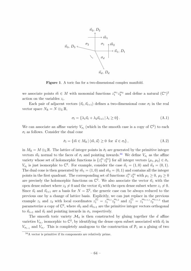
~n1, D1
~n2, D2
~n3, D3
~nd, Dd
~m1
~m2σ1σ2
σd
Figure 1. A toric fan for a two-dimensional complex manifold.
we associate points ~m ∈ M with monomial functions zm11 zm2
2 and define a natural (C∗)2
action on the variables zi.
Each pair of adjacent vectors (~nl, ~nl+1) defines a two-dimensional cone σl in the real
vector space NR = N ⊗Z R,
σl = λ1~nl + λ2~nl+1 |λi ≥ 0 . (A.1)
We can associate an affine variety Vσl (which in the smooth case is a copy of C2) to each
σl as follows. Consider the dual cone
σl = ~m ∈MR | 〈~m, ~u〉 ≥ 0 for ~u ∈ σl , (A.2)
in MR = M ⊗ZR. The lattice of integer points in σl are generated by the primitive integer
vectors ~ml normal to the faces of σl and pointing inwards.34 We define Vσl as the affine
variety whose set of holomorphic functions is zµ11 zµ22 for all integer vectors (µ1, µ2) ∈ σl.Vσl is just isomorphic to C2. For example, consider the case ~n1 = (1, 0) and ~n2 = (0, 1).
The dual cone is then generated by ~m1 = (1, 0) and ~m2 = (0, 1) and contains all the integer
points in the first quadrant. The corresponding set of functions zµ11 zµ22 with µ1 ≥ 0, µ2 ≥ 0
are precisely the holomorphic functions on C2. We also associate the vector ~n1 with the
open dense subset where z2 6= 0 and the vector ~n2 with the open dense subset where z1 6= 0.
Since ~nl and ~nl+1 are a basis for N = Z2, the generic case can be always reduced to the
previous one by a change of lattice basis. Explicitly, we can just replace in the previous
example z1 and z2 with local coordinates z(l)1 = z
ml,11 z
ml,22 and z
(l)2 = z
ml+1,1
1 zml+1,2
2 that
parameterize a copy of C2, where ~ml and ~ml+1 are the primitive integer vectors orthogonal
to ~nl+1 and ~nl and pointing inwards in σl, respectively.
The smooth toric variety M4 is then constructed by gluing together the d affine
varieties Vσl , isomorphic to C2, by identifying the dense open subset associated with ~nl in
Vσl−1and Vσl . This is completely analogous to the construction of P1 as a gluing of two
34A vector is primitive if its components are relatively prime.
– 64 –
copies of C. The action of the torus (C∗)2 on the variables z1 and z2 extends naturally to
a global action on V . Each chart Vσl contains a special point, the origin (0, 0) ∈ C2, which
is invariant under the torus action. These are the only invariant points and each of these
belongs precisely to one chart. We then see that there exactly are d fixed points under the
torus action (C∗)2, one for each of the two-dimensional cones σl.
Each vector ~nl determines a divisor Dl in M4 and a corresponding line bundle.35
There are precisely two relations among them given by
d∑l=1
〈~mk, ~nl〉Dl = 0 , k = 1, 2 , (A.3)
where ~m1 = (1, 0) and ~m2 = (0, 1) is a basis for M . This means that there are d − 2
independent two-cycles in M4. The intersection number of Dl and Dl′ , with l 6= l′, is one
if ~nl and ~nl′ are adjacent and otherwise is zero.
As we saw, the partition function onM4 × S1 localizes at the d fixed points of (C∗)2.
Each contributes a copy of the Nekrasov’s partition function of the corresponding chart
Vσl , twisted by the magnetic flux. The total magnetic flux is given by a divisor∑d
l=1 plDl
in M4, but the fixed point in the chart Vσl will only feel the contribution of the flux
coming from the divisors Dl and Dl+1. In the case of the chart C2, specified by the vectors
~n1 = (1, 0) and ~n2 = (0, 1), the local variables z1 and z2 parameterize the tangent space
around the fixed point z1 = z2 = 0. In this case we write a copy of the Nekrasov’s partition
function with equivariant parameters ε1 and ε2 and Coulomb variable a given by
a+ ε1p1 + ε2p2 . (A.4)
The replacement for a generic chart Vσl is then easily obtained. The equivariant parameters
are replaced by the action of (C∗)2 on the local parameters z(l)1 and z
(l)2 :
ε(l)1 = ~ml · ~ε , ε
(l)2 = ~ml+1 · ~ε , (A.5)
where ~ε = (ε1, ε2) and ~ml and ~ml+1 are the primitive integer vectors orthogonal to ~nl+1
and ~nl, respectively, and the Coulomb parameter by
a(l) = a+ ε(l)1 pl + ε
(l)2 pl+1 . (A.6)
We can also use toric geometry to evaluate the contribution of the magnetic flux to the
Hirzebruch-Riemann-Roch index. This can be done be evaluating (2.110) or using (2.111).
The two results obviously coincide, (2.110) being the localization formula for (2.111). For
completeness, let us also show how to evaluate (2.111) using toric geometry techniques.
In the case where E is a line bundle, the index (2.111) reads∫M4
ch(E)td(M4) = χ(M4) +
∫M4
(td1(P2)c1(E) +
1
2c1(E)2
). (A.7)
35In a local chart corresponding to ~n1 = (1, 0) and ~n2 = (0, 1), D1 restricts to z1 = 0 and D2 to z2 = 0.
– 65 –
We need the following general information about toric variety [72]. The holomorphic Euler
characteristic of every smooth toric four-manifold is one and c1(M4) is associated with
the divisor∑d
l=1Dl. We can then evaluate the integral of products of Chern classes with
the intersection of the corresponding divisors. Since td1(M4) = c1(M4)/2 and c1(E) =∑dl=1 plDl the index is given by
1 +1
2
( d∑l=1
plDl
)·( d∑
l=1
(pl + 1)Dl
). (A.8)
The intersection of divisors can be computed with the rules given above. For example, F1
is the toric manifold specified by the vectors ~n1 = (1, 0), ~n2 = (0, 1), ~n3 = (−1, 1) and
~n4 = (0,−1). The relations (A.3) gives D3 = D1 and D4 = D1 +D2. By combining these
relations with the fact that Di ·Dj = 1 if ~ni and ~nj are adjacent and Di ·Dj = 0 otherwise
(for i 6= j), we can determine the nonzero intersections among the independent divisors
D1 and D2: D21 = 0, D1 ·D2 = 1 and D2
2 = −1. We then easily obtain the index
1
2(p2 + p4 + 1)(2p1 − p2 + 2p3 + p4 + 2) , (A.9)
which correctly reproduces the results in example 2.3.
Notice that, by comparing (A.8) with (2.110), we can derive a general formula for the
self intersections of divisors
Dl ·Dl =
−(nl+1,1 + nl−1,1)/nl,1 , if nl,1 6= 0
−(nl+1,2 + nl−1,2)/nl,2 , if nl,2 6= 0. (A.10)
The two expressions agree when both conditions are met.
B Metric and spinor conventions
We work in Euclidean signature in five dimensions. We use m,n, p, . . . for spacetime and
a, b, c, . . . for tangent space indices. Spacetime indices are lowered and raised by gmn and
its inverse gmn. Tangent space indices are lowered and raised by δab and δab. Repeated
indices are summed. The two sets of indices are related using a vielbein e am , such that
gmn = e am e a
n . (B.1)
We define the Levi-Civita connection
Γmnp =
1
2gmt (∂ngtp + ∂pgnt − ∂tgnp) , (B.2)
and the spin connection
ω abm = e a
n ∇menb . (B.3)
– 66 –
The Riemann tensor is defined as
R abmn (e) = ∂mω
abn − ∂nω ab
m + ω acm ω b
nc − ω acm ω b
nc . (B.4)
The Ricci scalar is then given by
R(e) = enaemb R
abmn (e) . (B.5)
The spin group is Spin(5) ' USp(4). A spinor is a section ζα of the pseudo-real 4
representation of USp(4) with α ∈ 1, . . . , 4. The Clifford algebra is generated by Γ a
with a ∈ 1, . . . , 5 and Γ a, Γ b
= 2δab . (B.6)
The Γ matrices have index structure (Γ a)αβ. We define the Pauli matrices
τ 1 =
(0 1
1 0
), τ 2 =
(0 −ii 0
), τ 3 =
(1 0
0 −1
), (B.7)
and
σi = −σi = −iτ i , σ4 = σ4 = 12 . (B.8)
A possible choice of the Γ a is given by
Γ i =
(0 σi
σi 0
), i ∈ 1, . . . , 4 ,
Γ 5 = Γ 1Γ 2Γ 3Γ 4 =
(12 0
0 −12
).
(B.9)
We define the Γ matrices with multiple indices using permutations as
Γ a1a2...ap ≡ 1
p!
∑σ∈perm(p)
sign(σ)
p∏i=1
Γ aσ(i) , (B.10)
such that
Γ ab =1
2
(Γ aΓ b − Γ bΓ a
). (B.11)
We also define
σij ≡ 1
2(σiσj − σjσi) , σij ≡ 1
2(σiσj − σjσi) . (B.12)
The covariant derivatives for spinors are defined by
∇mξ = ∂mξ +1
4ω abm Γabξ . (B.13)
We also define a spinor Lie derivative along a Killing vector field v as
Lvξ ≡ vm∇mξ +1
2∇mvnΓ
mnξ . (B.14)
– 67 –
The Γ a satisfy
(Γ a)† = Γ a , (B.15)
where † denotes the conjugate transpose. We define a charge conjugation matrix
Cαβ ≡
(σ2 0
0 σ2
), (B.16)
satisfying
(Γ a)T = CΓ aC−1 , C∗ = C , C† = −C , C∗C = −14 , (B.17)
where T denotes transposition. Spinor bilinears are defined as
ξΓ a1a2...apη ≡ ξαCαβ (Γ a1a2...ap)βγ ηγ . (B.18)
The R-symmetry group of the five-dimensional N = 1 super-algebra is SU(2)R with
invariant antisymmetric tensor εIJ such that
ε12 = −ε21 = 1 . (B.19)
An SU(2) Majorana spinor is a doublet ζαI with I ∈ 1, 2 in the fundamental represen-
tation of SU(2)R satisfying the condition
ζ∗αI = Cαβε
IJζβJ . (B.20)
If the manifoldM4 is not spin, all spinors are valued instead in an appropriate bundle
associated with the choice of a spinc structure. This choice can be made canonically for an
almost complex manifold, but doing so may require a redefinition of certain background
fluxes. See [148] for examples in the context of localization and [149] for a complete
reference.
C Large N ’t Hooft anomalies of 4D/2D SCFTs from M5-branes
In this appendix we provide a simple formula, at large N , in order to extract the ’t
Hooft anomaly coefficients of four-dimensional N = 1 (or two-dimensional N = (0, 2)
field theories) that arise from M5-branes wrapped on a Riemann surface Σg2 (or a four-
manifold M4). The trial ’t Hooft anomaly coefficients of this class of theories can be
extracted by integrating the eight-form anomaly polynomial I8 of the 6D N = (2, 0)
theory over Σg2 orM4 [65, 66, 68, 150]. The anomaly eight-form of the 6D theory of type
g = (An≥1, Dn≥4, E6, E7, E8) reads [151–153]
I8[g] = rgI8[1] + dghgp2(NW )
24, (C.1)
– 68 –
where I8[1] is the anomaly eight-form of one M5-brane [154], NW is the SO(5) R-symmetry
bundle, and p2(NW ) is its second Pontryagin class. Here we have denoted the rank, the
dimension, and the Coxeter number of the Lie algebra g by rg, dg and hg, respectively. For
the AN−1 theory, in the large N limit, the anomaly eight-form is simply given by
I8[AN−1] ≈ N3
24e2
1e22 , (C.2)
where eς (ς = 1, 2) are the Chern roots of NW .
Let us first consider the compactification of 6D theories on a Riemann surface Σg2 .
The prescription in [65, 66] for computing the anomaly coefficient a(∆) of the 4D SCFT
amounts to first replace the Chern roots eς in (C.2) with
eς → −tς
2(1− g2)x+ ∆ςc1(F ) , (C.3)
implementing the topological twist along Σg2 , and then integrate the I8[AN−1] on Σg2 :
I6 =
∫Σg2
I8[AN−1] . (C.4)
Here x is the Chern root of the tangent bundle to Σg2 , c1(F ) is a flux coupled to the
R-symmetry, tς are the fluxes parameterizing the twist and ∆ς parameterize the trial
R-symmetry. They fulfill the following constraints
t1 + t2 = 2(1− g2) , ∆1 + ∆2 = 2 . (C.5)
On the other hand, the anomaly six-form of a 4D SCFT, at large N , reads
I6 ≈16
27a(∆)c1(F )3 . (C.6)
The ’t Hooft anomaly coefficient a(∆), at large N , where c = a, can then be read off by
expanding I8[AN−1] at first order in x, using (C.4) —∫Σg2
x = 2(1−g2) — and comparing
the result with (C.6). It is simply given by
a(∆) ≈ −9N3
128
2∑ς=1
tς∂(∆1∆2)2
∂∆ς
. (C.7)
This is (3.33) in the main text.
Consider now the compactification of 6D field theories on Σg1×Σg2 [68]. We first need
to replace
eς → −sς
2(1− g1)x1 −
tς2(1− g2)
x2 + ∆ςc1(F ) , (C.8)
where xς are now the Chern roots of the tangent bundles to Σgς , and tς/sς the fluxes on
Σg2/Σg1 , with
t1 + t2 = 2(1− g2) , s1 + s2 = 2(1− g1) . (C.9)
– 69 –
Then we integrate I8[AN−1] over Σg1 ×Σg2 using∫Σgς
x% = 2(1− gς)δς%. The result should
be compared with the four-form anomaly polynomial of the two-dimensional SCFT that,
in the large N limit, where cl = cr, reads
I4 ≈cl(∆)
6c1(F )2 . (C.10)
This time only the term proportional to x1x2 in (C.2) contributes and we obtain
cl(∆) ≈ N3
4
2∑ς,%=1
tςs%∂2(∆1∆2)2
∂∆ς∂∆%
. (C.11)
This is (3.12) with the identification β∆ς/π = ∆ς .
For completeness, we also study the compactification of 6D field theories on a four-
manifold M4 with a single flux on M4. Denoting with x1 and x2 the Chern roots of the
tangent bundle to M4, the topological twist can be implemented by [68]
eς → −rς(x1 + x2) + ∆ςc1(F ) , (C.12)
where r1 + r2 = 1. The integration of I8[AN−1] over M4 can be done by noticing that the
integrals
p1(M4) = 3 σ(M4) =
∫M4
(x21 + x2
2) , χ(M4) =
∫M4
x1x2 (C.13)
give the first Pontryagin number and the Euler number of M4. The result is then simply
cl(∆) ≈ N3
8(p1(M4) + 2χ(M4))
2∑ς,%=1
rςr%∂2(∆1∆2)2
∂∆ς∂∆%
. (C.14)
We see that the ’t Hooft anomaly coefficients of 4D (or 2D) field theories, which are
obtained by wrapping M5-branes on Σg2 (or M4), can always be written as (multiple)
applications of operators of the form∑2
ς=1 rς∂∆ς to the function (∆1∆2)2, appearing in
the eight-form anomaly polynomial through the term p2(NW ).
D An alternative large N saddle point for the USp(2N) theory
In this appendix, for completeness, we discuss a possible alternative method for evaluating
(3.8) in the saddle point approximation. Solving (3.9) in the large N limit gives a relation
between a(i) and ni. Eliminating a(i), we can write (3.8) as a sum over the fluxes ni:
ZpertΣg2×(Σg1×S1)(s, t, ∆) =
(−1)rk(G)
|W|∑n∈Γh
Zpert∣∣m=0
(a(n), n)
(detij
∂2Wpert(a(n), n)
∂ai∂aj
)g1−1
,
(D.1)
– 70 –
where a(i)(n) is the large N solution to (3.9). Each term in the sum is an exponentially
large function of N , and we can use again the saddle point approximation to find the
dominant contribution to the partition function. While for N = 2 SYM this method
fails since (3.9) completely fixes the values of ni, it works for the USp(2N) theory. For
completeness, we quote the result for the partition function evaluated with this approach
logZ(∆m, tm, sm) =4N5/2
5√
8−Nf
√(∆1t2 +∆2t1)(∆1s2 +∆2s1)(s1t2 + s2t1) . (D.2)
Notice that this is different from (3.106). It coincides with (3.106) only in the case of the
universal twist, tm = 1 − g2 and sm = 1 − g1. It would be very interesting to compare
the two alternative results with the entropy of asymptotically AdS6 black holes in massive
type IIA supergravity, with magnetic fluxes tm and sm [69].
E Polylogarithms
Polylogarithms Lis(z) are defined by
Lis(z) =∞∑n=1
zn
ns, (E.1)
for |z| < 1 and by analytic continuation outside the disk. They satisfy the following
relations
∂a Lis(eia) = iLis−1(eia) , Lis(e
ia) = i
∫ a
+i∞Lis−1(eia
′) da′ . (E.2)
For s ≥ 1, the functions have a branch point at z = 1 and we shall take the principal
determination with a cut [1,+∞) along the real axis. The functions Lis(eia) are periodic
under a→ a+ 2π and have branch cut discontinuities along the vertical line [0,−i∞) and
its images. For 0 < Re a < 2π, polylogarithms fulfill the following inversion formula36
Lis(eia) + (−1)s Lis(e
−ia) = −(2iπ)s
s!Bs
( a2π
)≡ i
s−2gs(a) , (E.3)
where Bs(a) are the Bernoulli polynomials. In this paper we need, in particular,
g2(a) =a2
2− πa+
π2
3, g3(a) =
a3
6− π
2a2 +
π2
3a . (E.4)
One can find the formulæ in the other regions by periodicity. Let us also mention that
gs(2π − a) = (−1)sgs(a) . (E.5)
Finally, assuming 0 < ∆ < 2π, we find that
Lis(et+i∆) ∼ i
s−2gs(−it+∆) , as t→∞ . (E.6)36The inversion formulæ in the domain −2π < Re a < 0 are obtained by sending a→ −a.
– 71 –
References
[1] E. Witten, “Topological Quantum Field Theory,” Commun. Math. Phys. 117 (1988) 353.
[2] E. Witten, “Mirror manifolds and topological field theory,” arXiv:hep-th/9112056
[hep-th]. [AMS/IP Stud. Adv. Math.9,121(1998)].
[3] V. Pestun, “Localization of gauge theory on a four-sphere and supersymmetric Wilson
loops,” Commun. Math. Phys. 313 (2012) 71–129, arXiv:0712.2824 [hep-th].
[4] F. Benini and A. Zaffaroni, “A topologically twisted index for three-dimensional
supersymmetric theories,” JHEP 07 (2015) 127, arXiv:1504.03698 [hep-th].
[5] F. Benini, K. Hristov, and A. Zaffaroni, “Black hole microstates in AdS4 from
supersymmetric localization,” JHEP 05 (2016) 054, arXiv:1511.04085 [hep-th].
[6] S. Okuda and Y. Yoshida, “G/G gauged WZW model and Bethe Ansatz for the phase
model,” JHEP 11 (2012) 146, arXiv:1209.3800 [hep-th].
[7] S. Okuda and Y. Yoshida, “G/G gauged WZW-matter model, Bethe Ansatz for q-boson
model and Commutative Frobenius algebra,” JHEP 03 (2014) 003, arXiv:1308.4608
[hep-th].
[8] N. A. Nekrasov and S. L. Shatashvili, “Bethe/Gauge correspondence on curved spaces,”
JHEP 01 (2015) 100, arXiv:1405.6046 [hep-th].
[9] S. Gukov and D. Pei, “Equivariant Verlinde formula from fivebranes and vortices,”
Commun. Math. Phys. 355 no. 1, (2017) 1–50, arXiv:1501.01310 [hep-th].
[10] S. Okuda and Y. Yoshida, “Gauge/Bethe correspondence on S1 ×Σh and index over
moduli space,” arXiv:1501.03469 [hep-th].
[11] S. Gukov, P. Putrov, and C. Vafa, “Fivebranes and 3-manifold homology,” JHEP 07
(2017) 071, arXiv:1602.05302 [hep-th].
[12] C. Closset and H. Kim, “Comments on twisted indices in 3d supersymmetric gauge
theories,” JHEP 08 (2016) 059, arXiv:1605.06531 [hep-th].
[13] C. Closset, H. Kim, and B. Willett, “Supersymmetric partition functions and the
three-dimensional A-twist,” JHEP 03 (2017) 074, arXiv:1701.03171 [hep-th].
[14] M. Dedushenko, S. Gukov, and P. Putrov, “Vertex algebras and 4-manifold invariants,”
arXiv:1705.01645 [hep-th].
[15] S. Gukov, “Trisecting non-Lagrangian theories,” JHEP 11 (2017) 178,
arXiv:1707.01515 [hep-th].
[16] C. Closset, H. Kim, and B. Willett, “N = 1 supersymmetric indices and the
four-dimensional A-model,” JHEP 08 (2017) 090, arXiv:1707.05774 [hep-th].
[17] C. Closset, H. Kim, and B. Willett, “Seifert fibering operators in 3d N = 2 theories,”
arXiv:1807.02328 [hep-th].
[18] F. Benini and A. Zaffaroni, “Supersymmetric partition functions on Riemann surfaces,”
Proc. Symp. Pure Math. 96 (2017) 13–46, arXiv:1605.06120 [hep-th].
– 72 –
[19] S. L. Cacciatori and D. Klemm, “Supersymmetric AdS(4) black holes and attractors,”
JHEP 01 (2010) 085, arXiv:0911.4926 [hep-th].
[20] G. Dall’Agata and A. Gnecchi, “Flow equations and attractors for black holes in N = 2
U(1) gauged supergravity,” JHEP 03 (2011) 037, arXiv:1012.3756 [hep-th].
[21] K. Hristov and S. Vandoren, “Static supersymmetric black holes in AdS4 with spherical
symmetry,” JHEP 04 (2011) 047, arXiv:1012.4314 [hep-th].
[22] S. Katmadas, “Static BPS black holes in U(1) gauged supergravity,” JHEP 09 (2014)
027, arXiv:1405.4901 [hep-th].
[23] N. Halmagyi, “Static BPS black holes in AdS4 with general dyonic charges,” JHEP 03
(2015) 032, arXiv:1408.2831 [hep-th].
[24] F. Benini, K. Hristov, and A. Zaffaroni, “Exact microstate counting for dyonic black
holes in AdS4,” Phys. Lett. B771 (2017) 462–466, arXiv:1608.07294 [hep-th].
[25] O. Aharony, O. Bergman, D. L. Jafferis, and J. Maldacena, “N=6 superconformal
Chern-Simons-matter theories, M2-branes and their gravity duals,” JHEP 10 (2008) 091,
arXiv:0806.1218 [hep-th].
[26] S. M. Hosseini, A. Nedelin, and A. Zaffaroni, “The Cardy limit of the topologically
twisted index and black strings in AdS5,” JHEP 04 (2017) 014, arXiv:1611.09374
[hep-th].
[27] S. M. Hosseini, Black hole microstates and supersymmetric localization. PhD thesis,
Milan Bicocca U., 2018-02. arXiv:1803.01863 [hep-th].
[28] J. Hong and J. T. Liu, “The topologically twisted index of N = 4 super-Yang-Mills on
T 2 × S2 and the elliptic genus,” arXiv:1804.04592 [hep-th].
[29] A. Cabo-Bizet, V. I. Giraldo-Rivera, and L. A. Pando Zayas, “Microstate counting of
AdS4 hyperbolic black hole entropy via the topologically twisted index,” JHEP 08 (2017)
023, arXiv:1701.07893 [hep-th].
[30] F. Azzurli, N. Bobev, P. M. Crichigno, V. S. Min, and A. Zaffaroni, “A universal counting
of black hole microstates in AdS4,” JHEP 02 (2018) 054, arXiv:1707.04257 [hep-th].
[31] S. M. Hosseini, K. Hristov, and A. Passias, “Holographic microstate counting for AdS4
black holes in massive IIA supergravity,” JHEP 10 (2017) 190, arXiv:1707.06884
[hep-th].
[32] F. Benini, H. Khachatryan, and P. Milan, “Black hole entropy in massive Type IIA,”
Class. Quant. Grav. 35 no. 3, (2018) 035004, arXiv:1707.06886 [hep-th].
[33] N. Bobev, V. S. Min, and K. Pilch, “Mass-deformed ABJM and black holes in AdS4,”
JHEP 03 (2018) 050, arXiv:1801.03135 [hep-th].
[34] C. Toldo and B. Willett, “Partition functions on 3d circle bundles and their gravity
duals,” JHEP 05 (2018) 116, arXiv:1712.08861 [hep-th].
[35] D. Gang and N. Kim, “Large N twisted partition functions in 3d-3d correspondence and
Holography,” arXiv:1808.02797 [hep-th].
– 73 –
[36] J. T. Liu, L. A. Pando Zayas, V. Rathee, and W. Zhao, “One-Loop Test of Quantum
Black Holes in anti de Sitter Space,” Phys. Rev. Lett. 120 no. 22, (2018) 221602,
arXiv:1711.01076 [hep-th].
[37] J. T. Liu, L. A. Pando Zayas, V. Rathee, and W. Zhao, “Toward Microstate Counting
Beyond Large N in Localization and the Dual One-loop Quantum Supergravity,” JHEP
01 (2018) 026, arXiv:1707.04197 [hep-th].
[38] I. Jeon and S. Lal, “Logarithmic Corrections to Entropy of Magnetically Charged AdS4
Black Holes,” Phys. Lett. B774 (2017) 41–45, arXiv:1707.04208 [hep-th].
[39] N. Halmagyi and S. Lal, “On the on-shell: the action of AdS4 black holes,” JHEP 03
(2018) 146, arXiv:1710.09580 [hep-th].
[40] A. Cabo-Bizet, U. Kol, L. A. Pando Zayas, I. Papadimitriou, and V. Rathee, “Entropy
functional and the holographic attractor mechanism,” JHEP 05 (2018) 155,
arXiv:1712.01849 [hep-th].
[41] K. Hristov, I. Lodato, and V. Reys, “On the quantum entropy function in 4d gauged
supergravity,” arXiv:1803.05920 [hep-th].
[42] J. Nian and X. Zhang, “Entanglement Entropy of ABJM Theory and Entropy of
Topological Black Hole,” JHEP 07 (2017) 096, arXiv:1705.01896 [hep-th].
[43] S. M. Hosseini, K. Hristov, and A. Zaffaroni, “An extremization principle for the entropy
of rotating BPS black holes in AdS5,” JHEP 07 (2017) 106, arXiv:1705.05383
[hep-th].
[44] S. M. Hosseini, K. Hristov, and A. Zaffaroni, “A note on the entropy of rotating BPS
AdS7 × S4 black holes,” JHEP 05 (2018) 121, arXiv:1803.07568 [hep-th].
[45] F. Benini and N. Bobev, “Exact two-dimensional superconformal R-symmetry and
c-extremization,” Phys. Rev. Lett. 110 no. 6, (2013) 061601, arXiv:1211.4030
[hep-th].
[46] S. M. Hosseini and A. Zaffaroni, “Large N matrix models for 3d N = 2 theories: twisted
index, free energy and black holes,” JHEP 08 (2016) 064, arXiv:1604.03122 [hep-th].
[47] S. M. Hosseini and N. Mekareeya, “Large N topologically twisted index: necklace
quivers, dualities, and Sasaki-Einstein spaces,” JHEP 08 (2016) 089, arXiv:1604.03397
[hep-th].
[48] C. P. Herzog, I. R. Klebanov, S. S. Pufu, and T. Tesileanu, “Multi-Matrix Models and
Tri-Sasaki Einstein Spaces,” Phys. Rev. D83 (2011) 046001, arXiv:1011.5487
[hep-th].
[49] D. L. Jafferis, I. R. Klebanov, S. S. Pufu, and B. R. Safdi, “Towards the F-Theorem: N=2
Field Theories on the Three-Sphere,” JHEP 06 (2011) 102, arXiv:1103.1181 [hep-th].
[50] M. Fluder and J. Sparks, “D2-brane Chern-Simons theories: F-maximization =
a-maximization,” JHEP 01 (2016) 048, arXiv:1507.05817 [hep-th].
– 74 –
[51] H.-C. Kim and K. Lee, “Supersymmetric M5 Brane Theories on R x CP2,” JHEP 07
(2013) 072, arXiv:1210.0853 [hep-th].
[52] H.-C. Kim, S. Kim, S.-S. Kim, and K. Lee, “The general M5-brane superconformal
index,” arXiv:1307.7660 [hep-th].
[53] N. A. Nekrasov, “Localizing gauge theories,” in Mathematical physics. Proceedings, 14th
International Congress, ICMP 2003, Lisbon, Portugal, July 28-August 2, 2003,
pp. 645–654. 2003.
[54] A. Bawane, G. Bonelli, M. Ronzani, and A. Tanzini, “N = 2 supersymmetric gauge
theories on S2 × S2 and Liouville Gravity,” JHEP 07 (2015) 054, arXiv:1411.2762
[hep-th].
[55] M. Bershtein, G. Bonelli, M. Ronzani, and A. Tanzini, “Exact results for N = 2
supersymmetric gauge theories on compact toric manifolds and equivariant Donaldson
invariants,” JHEP 07 (2016) 023, arXiv:1509.00267 [hep-th].
[56] M. Bershtein, G. Bonelli, M. Ronzani, and A. Tanzini, “Gauge theories on compact toric
surfaces, conformal field theories and equivariant Donaldson invariants,” J. Geom. Phys.
118 (2017) 40–50, arXiv:1606.07148 [hep-th].
[57] N. Seiberg, “Five-dimensional SUSY field theories, nontrivial fixed points and string
dynamics,” Phys. Lett. B388 (1996) 753–760, arXiv:hep-th/9608111 [hep-th].
[58] A. Brandhuber and Y. Oz, “The D-4 - D-8 brane system and five-dimensional fixed
points,” Phys. Lett. B460 (1999) 307–312, arXiv:hep-th/9905148 [hep-th].
[59] M. R. Douglas, “On D=5 super Yang-Mills theory and (2,0) theory,” JHEP 02 (2011)
011, arXiv:1012.2880 [hep-th].
[60] N. Lambert, C. Papageorgakis, and M. Schmidt-Sommerfeld, “M5-Branes, D4-Branes
and Quantum 5D super-Yang-Mills,” JHEP 01 (2011) 083, arXiv:1012.2882 [hep-th].
[61] S. Bolognesi and K. Lee, “Instanton Partons in 5-dim SU(N) Gauge Theory,” Phys. Rev.
D84 (2011) 106001, arXiv:1106.3664 [hep-th].
[62] H.-C. Kim and S. Kim, “M5-branes from gauge theories on the 5-sphere,” JHEP 05
(2013) 144, arXiv:1206.6339 [hep-th].
[63] N. Nekrasov, “Five dimensional gauge theories and relativistic integrable systems,” Nucl.
Phys. B531 (1998) 323–344, arXiv:hep-th/9609219 [hep-th].
[64] I. Bah, A. Passias, and P. Weck, “Holographic duals of five-dimensional SCFTs on a
Riemann surface,” arXiv:1807.06031 [hep-th].
[65] I. Bah, C. Beem, N. Bobev, and B. Wecht, “AdS/CFT Dual Pairs from M5-Branes on
Riemann Surfaces,” Phys. Rev. D85 (2012) 121901, arXiv:1112.5487 [hep-th].
[66] I. Bah, C. Beem, N. Bobev, and B. Wecht, “Four-Dimensional SCFTs from M5-Branes,”
JHEP 06 (2012) 005, arXiv:1203.0303 [hep-th].
[67] P. M. Crichigno, D. Jain, and B. Willett, “5d Partition Functions with A Twist,”
arXiv:1808.06744 [hep-th].
– 75 –
[68] F. Benini and N. Bobev, “Two-dimensional SCFTs from wrapped branes and
c-extremization,” JHEP 06 (2013) 005, arXiv:1302.4451 [hep-th].
[69] S. M. Hosseini, K. Hristov, A. Passias, and A. Zaffaroni, “in progress,”.
[70] M. Abreu, “Kahler geometry of toric manifolds in symplectic coordinates,” ArXiv
Mathematics e-prints (Apr., 2000) , math/0004122.
[71] V. Guillemin, “Kaehler structures on toric varieties,” J. Differential Geom. 40 no. 2,
(1994) 285–309.
[72] W. Fulton, Introduction to Toric Varieties. Annals of mathematics studies. Princeton
University Press, 1993.
[73] N. A. Nekrasov, “Seiberg-Witten prepotential from instanton counting,” Adv. Theor.
Math. Phys. 7 no. 5, (2003) 831–864, arXiv:hep-th/0206161 [hep-th].
[74] N. Nekrasov and A. Okounkov, “Seiberg-Witten theory and random partitions,” Prog.
Math. 244 (2006) 525–596, arXiv:hep-th/0306238 [hep-th].
[75] G. Festuccia and N. Seiberg, “Rigid Supersymmetric Theories in Curved Superspace,”
JHEP 06 (2011) 114, arXiv:1105.0689 [hep-th].
[76] T. T. Dumitrescu, G. Festuccia, and N. Seiberg, “Exploring Curved Superspace,” JHEP
08 (2012) 141, arXiv:1205.1115 [hep-th].
[77] C. Klare, A. Tomasiello, and A. Zaffaroni, “Supersymmetry on Curved Spaces and
Holography,” JHEP 08 (2012) 061, arXiv:1205.1062 [hep-th].
[78] C. Klare and A. Zaffaroni, “Extended Supersymmetry on Curved Spaces,” JHEP 10
(2013) 218, arXiv:1308.1102 [hep-th].
[79] D. Rodriguez-Gomez and J. Schmude, “Partition functions for equivariantly twisted
N = 2 gauge theories on toric Kahler manifolds,” JHEP 05 (2015) 111,
arXiv:1412.4407 [hep-th].
[80] L. F. Alday, P. Benetti Genolini, M. Fluder, P. Richmond, and J. Sparks,
“Supersymmetric gauge theories on five-manifolds,” JHEP 08 (2015) 007,
arXiv:1503.09090 [hep-th].
[81] A. Pini, D. Rodriguez-Gomez, and J. Schmude, “Rigid Supersymmetry from Conformal
Supergravity in Five Dimensions,” JHEP 09 (2015) 118, arXiv:1504.04340 [hep-th].
[82] B. de Wit and V. Reys, “Euclidean supergravity,” JHEP 12 (2017) 011,
arXiv:1706.04973 [hep-th].
[83] K. Hosomichi, R.-K. Seong, and S. Terashima, “Supersymmetric Gauge Theories on the
Five-Sphere,” Nucl. Phys. B865 (2012) 376–396, arXiv:1203.0371 [hep-th].
[84] J. Kallen, J. Qiu, and M. Zabzine, “The perturbative partition function of
supersymmetric 5D Yang-Mills theory with matter on the five-sphere,” JHEP 08 (2012)
157, arXiv:1206.6008 [hep-th].
[85] J. Qiu and M. Zabzine, “Review of localization for 5d supersymmetric gauge theories,” J.
Phys. A50 no. 44, (2017) 443014, arXiv:1608.02966 [hep-th].
– 76 –
[86] J. Kallen and M. Zabzine, “Twisted supersymmetric 5D Yang-Mills theory and contact
geometry,” JHEP 05 (2012) 125, arXiv:1202.1956 [hep-th].
[87] J. Qiu and M. Zabzine, “5D Super Yang-Mills on Y p,q Sasaki-Einstein manifolds,”
Commun. Math. Phys. 333 no. 2, (2015) 861–904, arXiv:1307.3149 [hep-th].
[88] M. F. Atiyah, N. J. Hitchin, and I. M. Singer, “Selfduality in Four-Dimensional
Riemannian Geometry,” Proc. Roy. Soc. Lond. A362 (1978) 425–461.
[89] C. Closset, S. Cremonesi, and D. S. Park, “The equivariant A-twist and gauged linear
sigma models on the two-sphere,” JHEP 06 (2015) 076, arXiv:1504.06308 [hep-th].
[90] F. Benini, R. Eager, K. Hori, and Y. Tachikawa, “Elliptic genera of two-dimensional N=2
gauge theories with rank-one gauge groups,” Lett. Math. Phys. 104 (2014) 465–493,
arXiv:1305.0533 [hep-th].
[91] K. Hori, H. Kim, and P. Yi, “Witten Index and Wall Crossing,” JHEP 01 (2015) 124,
arXiv:1407.2567 [hep-th].
[92] L. C. Jeffrey and F. C. Kirwan, “Localization for nonabelian group actions,” Topology 34
(1995) 291–327, arXiv:alg-geom/9307001.
[93] C. Hwang, J. Kim, S. Kim, and J. Park, “General instanton counting and 5d SCFT,”
JHEP 07 (2015) 063, arXiv:1406.6793 [hep-th]. [Addendum: JHEP04,094(2016)].
[94] J. Gomis, T. Okuda, and V. Pestun, “Exact Results for ’t Hooft Loops in Gauge
Theories on S4,” JHEP 05 (2012) 141, arXiv:1105.2568 [hep-th].
[95] M. Atiyah, Elliptic Operators and Compact Groups. Lecture Notes in Mathematics.
Springer Berlin Heidelberg, 2006.
[96] V. Pestun, “Review of localization in geometry,” J. Phys. A50 no. 44, (2017) 443002,
arXiv:1608.02954 [hep-th].
[97] V. Pestun and M. Zabzine, “Introduction to localization in quantum field theory,” J.
Phys. A50 no. 44, (2017) 443001, arXiv:1608.02953 [hep-th].
[98] M. Marino, The Geometry of supersymmetric gauge theories in four-dimensions. PhD
thesis, Santiago de Compostela U., 1997. arXiv:hep-th/9701128 [hep-th].
[99] H.-C. Kim, S. Kim, E. Koh, K. Lee, and S. Lee, “On instantons as Kaluza-Klein modes
of M5-branes,” JHEP 12 (2011) 031, arXiv:1110.2175 [hep-th].
[100] M. Bullimore and H.-C. Kim, “The Superconformal Index of the (2,0) Theory with
Defects,” JHEP 05 (2015) 048, arXiv:1412.3872 [hep-th].
[101] T. Nishioka and I. Yaakov, “Supersymmetric Renyi entropy and defect operators,” JHEP
11 (2017) 071, arXiv:1612.02894 [hep-th].
[102] T. Okuda and V. Pestun, “On the instantons and the hypermultiplet mass of N=2*
super Yang-Mills on S4,” JHEP 03 (2012) 017, arXiv:1004.1222 [hep-th].
[103] C. Vafa and E. Witten, “A Strong coupling test of S duality,” Nucl. Phys. B431 (1994)
3–77, arXiv:hep-th/9408074 [hep-th].
– 77 –
[104] L. Gottsche, H. Nakajima, and K. Yoshioka, “K-theoretic Donaldson invariants via
instanton counting,” Pure Appl. Math. Quart. 5 (2009) 1029–1111, arXiv:math/0611945
[math-ag].
[105] M. Bershtein, P. Gavrylenko, and A. Marshakov, “Cluster Toda chains and Nekrasov
functions,” arXiv:1804.10145 [math-ph].
[106] H. Nakajima and K. Yoshioka, “Instanton counting on blowup. II. K-theoretic partition
function,” arXiv:math/0505553 [math-ag].
[107] Y. Tachikawa, “Five-dimensional Chern-Simons terms and Nekrasov’s instanton
counting,” JHEP 02 (2004) 050, arXiv:hep-th/0401184 [hep-th].
[108] Y. Tachikawa, “A review on instanton counting and W-algebras,” in New Dualities of
Supersymmetric Gauge Theories, J. Teschner, ed., pp. 79–120. 2016. arXiv:1412.7121
[hep-th].
[109] J. Qiu, L. Tizzano, J. Winding, and M. Zabzine, “Gluing Nekrasov partition functions,”
Commun. Math. Phys. 337 no. 2, (2015) 785–816, arXiv:1403.2945 [hep-th].
[110] F. Nieri, S. Pasquetti, and F. Passerini, “3d and 5d Gauge Theory Partition Functions as
q-deformed CFT Correlators,” Lett. Math. Phys. 105 no. 1, (2015) 109–148,
arXiv:1303.2626 [hep-th].
[111] S. Pasquetti, “Holomorphic blocks and the 5d AGT correspondence,” J. Phys. A50
no. 44, (2017) 443016, arXiv:1608.02968 [hep-th].
[112] M. Kool, “Euler characteristics of moduli spaces of torsion free sheaves on toric
surfaces,” Geometriae Dedicata 176 no. 1, (Jun, 2015) 241–269.
[113] F. Benini, N. Bobev, and P. M. Crichigno, “Two-dimensional SCFTs from D3-branes,”
JHEP 07 (2016) 020, arXiv:1511.09462 [hep-th].
[114] N. Bobev and P. M. Crichigno, “Universal RG Flows Across Dimensions and
Holography,” JHEP 12 (2017) 065, arXiv:1708.05052 [hep-th].
[115] G. W. Moore and E. Witten, “Integration over the u plane in Donaldson theory,” Adv.
Theor. Math. Phys. 1 (1997) 298–387, arXiv:hep-th/9709193 [hep-th].
[116] N. A. Nekrasov and S. L. Shatashvili, “Quantization of Integrable Systems and Four
Dimensional Gauge Theories,” in Proceedings, 16th International Congress on
Mathematical Physics (ICMP09): Prague, Czech Republic, August 3-8, 2009,
pp. 265–289. 2009. arXiv:0908.4052 [hep-th].
[117] N. Nekrasov and E. Witten, “The Omega Deformation, Branes, Integrability, and
Liouville Theory,” JHEP 09 (2010) 092, arXiv:1002.0888 [hep-th].
[118] Y. Luo, M.-C. Tan, and J. Yagi, “N = 2 supersymmetric gauge theories and quantum
integrable systems,” JHEP 03 (2014) 090, arXiv:1310.0827 [hep-th].
[119] N. A. Nekrasov and S. L. Shatashvili, “Supersymmetric vacua and Bethe ansatz,” Nucl.
Phys. Proc. Suppl. 192-193 (2009) 91–112, arXiv:0901.4744 [hep-th].
– 78 –
[120] E. Witten, “Some comments on string dynamics,” in Future perspectives in string theory.
Proceedings, Conference, Strings’95, Los Angeles, USA, March 13-18, 1995, pp. 501–523.
1995. arXiv:hep-th/9507121 [hep-th].
[121] A. Strominger, “Open p-branes,” Phys. Lett. B383 (1996) 44–47,
arXiv:hep-th/9512059 [hep-th]. [,116(1995)].
[122] J. A. Minahan, A. Nedelin, and M. Zabzine, “5D super Yang-Mills theory and the
correspondence to AdS7/CFT6,” J. Phys. A46 (2013) 355401, arXiv:1304.1016
[hep-th].
[123] J. L. Cardy, “Operator Content of Two-Dimensional Conformally Invariant Theories,”
Nucl. Phys. B270 (1986) 186–204.
[124] K. A. Intriligator, D. R. Morrison, and N. Seiberg, “Five-dimensional supersymmetric
gauge theories and degenerations of Calabi-Yau spaces,” Nucl. Phys. B497 (1997)
56–100, arXiv:hep-th/9702198 [hep-th].
[125] O. Bergman and D. Rodriguez-Gomez, “5d quivers and their AdS(6) duals,” JHEP 07
(2012) 171, arXiv:1206.3503 [hep-th].
[126] D. R. Morrison and N. Seiberg, “Extremal transitions and five-dimensional
supersymmetric field theories,” Nucl. Phys. B483 (1997) 229–247,
arXiv:hep-th/9609070 [hep-th].
[127] D. L. Jafferis and S. S. Pufu, “Exact results for five-dimensional superconformal field
theories with gravity duals,” JHEP 05 (2014) 032, arXiv:1207.4359 [hep-th].
[128] C.-M. Chang, M. Fluder, Y.-H. Lin, and Y. Wang, “Romans Supergravity from
Five-Dimensional Holograms,” arXiv:1712.10313 [hep-th].
[129] D. L. Jafferis, “The Exact Superconformal R-Symmetry Extremizes Z,” JHEP 05 (2012)
159, arXiv:1012.3210 [hep-th].
[130] M. Naka, “Various wrapped branes from gauged supergravities,” arXiv:hep-th/0206141
[hep-th].
[131] M. Suh, “D4-branes wrapped on a supersymmetric four-cycle,” arXiv:1809.03517
[hep-th].
[132] S. Ferrara, R. Kallosh, and A. Strominger, “N=2 extremal black holes,” Phys. Rev. D52
(1995) R5412–R5416, arXiv:hep-th/9508072 [hep-th].
[133] S. Ferrara and R. Kallosh, “Supersymmetry and attractors,” Phys. Rev. D54 (1996)
1514–1524, arXiv:hep-th/9602136 [hep-th].
[134] J. M. Maldacena and C. Nunez, “Supergravity description of field theories on curved
manifolds and a no go theorem,” Int. J. Mod. Phys. A16 (2001) 822–855,
arXiv:hep-th/0007018 [hep-th]. [,182(2000)].
[135] J. T. Liu and R. Minasian, “Black holes and membranes in AdS(7),” Phys. Lett. B457
(1999) 39–46, arXiv:hep-th/9903269 [hep-th].
– 79 –
[136] M. Pernici, K. Pilch, and P. van Nieuwenhuizen, “Gauged Maximally Extended
Supergravity in Seven-dimensions,” Phys. Lett. 143B (1984) 103–107.
[137] H. Nastase, D. Vaman, and P. van Nieuwenhuizen, “Consistent nonlinear K K reduction
of 11-d supergravity on AdS(7) x S(4) and selfduality in odd dimensions,” Phys. Lett.
B469 (1999) 96–102, arXiv:hep-th/9905075 [hep-th].
[138] H. Nastase, D. Vaman, and P. van Nieuwenhuizen, “Consistency of the AdS(7) x S(4)
reduction and the origin of selfduality in odd dimensions,” Nucl. Phys. B581 (2000)
179–239, arXiv:hep-th/9911238 [hep-th].
[139] J. D. Brown and M. Henneaux, “Central charges in the canonical realization of
asymptotic symmetries: An example from three dimensional gravity,” Communications
in Mathematical Physics 104 no. 2, (Jun, 1986) 207–226.
[140] A. Amariti and C. Toldo, “Betti multiplets, flows across dimensions and
c-extremization,” JHEP 07 (2017) 040, arXiv:1610.08858 [hep-th].
[141] K. Hristov, “Dimensional reduction of BPS attractors in AdS gauged supergravities,”
JHEP 12 (2014) 066, arXiv:1409.8504 [hep-th].
[142] D. Klemm, N. Petri, and M. Rabbiosi, “Symplectically invariant flow equations for
N = 2, D = 4 gauged supergravity with hypermultiplets,” JHEP 04 (2016) 008,
arXiv:1602.01334 [hep-th].
[143] P. Szepietowski, “Comments on a-maximization from gauged supergravity,” JHEP 12
(2012) 018, arXiv:1209.3025 [hep-th].
[144] Y. Tachikawa, “Five-dimensional supergravity dual of a-maximization,” Nucl. Phys.
B733 (2006) 188–203, arXiv:hep-th/0507057 [hep-th].
[145] M. Banados, C. Teitelboim, and J. Zanelli, “The Black hole in three-dimensional
space-time,” Phys. Rev. Lett. 69 (1992) 1849–1851, arXiv:hep-th/9204099 [hep-th].
[146] O. Bergman, D. Rodriguez-Gomez, and G. Zafrir, “5-Brane Webs, Symmetry
Enhancement, and Duality in 5d Supersymmetric Gauge Theory,” JHEP 03 (2014) 112,
arXiv:1311.4199 [hep-th].
[147] O. Bergman and G. Zafrir, “5d fixed points from brane webs and O7-planes,” JHEP 12
(2015) 163, arXiv:1507.03860 [hep-th].
[148] G. Festuccia, J. Qiu, J. Winding, and M. Zabzine, “N = 2 supersymmetric gauge theory
on connected sums of S2 × S2,” JHEP 03 (2017) 026, arXiv:1611.04868 [hep-th].
[149] D. Salamon, “Spin geometry and seiberg-witten invariants,” 1996.
[150] L. F. Alday, F. Benini, and Y. Tachikawa, “Liouville/Toda central charges from
M5-branes,” Phys. Rev. Lett. 105 (2010) 141601, arXiv:0909.4776 [hep-th].
[151] J. A. Harvey, R. Minasian, and G. W. Moore, “NonAbelian tensor multiplet anomalies,”
JHEP 09 (1998) 004, arXiv:hep-th/9808060 [hep-th].
[152] K. A. Intriligator, “Anomaly matching and a Hopf-Wess-Zumino term in 6d, N=(2,0)
field theories,” Nucl. Phys. B581 (2000) 257–273, arXiv:hep-th/0001205 [hep-th].
– 80 –
[153] P. Yi, “Anomaly of (2,0) theories,” Phys. Rev. D64 (2001) 106006,
arXiv:hep-th/0106165 [hep-th].
[154] E. Witten, “Five-brane effective action in M theory,” J. Geom. Phys. 22 (1997) 103–133,
arXiv:hep-th/9610234 [hep-th].
– 81 –


![TOPOLOGICALLY SLICE KNOTS WITH NONTRIVIAL ...arXiv:1001.1538v3 [math.GT] 7 May 2011 TOPOLOGICALLY SLICE KNOTS WITH NONTRIVIAL ALEXANDER POLYNOMIAL MATTHEW HEDDEN, CHARLES LIVINGSTON,](https://img.pdfslide.net/doc/110x75/5f8d8100ff950450d4784567/topologically-slice-knots-with-nontrivial-arxiv10011538v3-mathgt-7-may.jpg)


![Adaptive Cube Tessellation for Topologically Correct ... · Adaptive Cube Tessellation for Topologically Correct Isosurfaces ... [PT90]. This method is ... Tessellation for Topologically](https://img.pdfslide.net/doc/110x75/5adfba127f8b9a5a668ca39b/adaptive-cube-tessellation-for-topologically-correct-cube-tessellation-for-topologically.jpg)


![in topologically nontrivial spacesarXiv:1507.08832v1 [hep-th] 31 Jul 2015 Casimir effect for scalar current densities in topologically nontrivial spaces S.Bellucci1∗,A.A.Saharian](https://img.pdfslide.net/doc/110x75/606cb78760e9502f474e0167/in-topologically-nontrivial-spaces-arxiv150708832v1-hep-th-31-jul-2015-casimir.jpg)