Embed Size (px)
Citation preview
International Journal of Solids and Structures 43 (2006) 5307–5336
www.elsevier.com/locate/ijsolstr
Torsion of closed section, orthotropic, thin-walled beams
Aniko Pluzsik, Laszlo P. Kollar *
Department of Mechanics, Materials and Structures, Budapest University of Technology and Economics,
Muegyetem rkpt. 1, 1521, Hungary
Received 22 April 2005Available online 6 October 2005
Abstract
The paper presents a theory for thin-walled, closed section, orthotropic beams which takes into account the sheardeformation in restrained warping induced torque. In the derivation we developed the analytical (‘‘exact’’) solutionof simply supported beams subjected to a sinusoidal load. The replacement stiffnesses which are independent of thelength of the beam were determined from the exact solution by taking its Taylor series expansion with respect to theinverse of the length of the beam. The effect of restrained warping and shear deformation was investigated throughnumerical examples.� 2005 Elsevier Ltd. All rights reserved.
Keywords: Composite; Closed section; Beam theory; Torsion; Restrained warping
1. Introduction
Fiber reinforced plastic (composite), thin-walled beams are widely used in the aerospace industry and areincreasingly applied in the infrastructure. Thin-walled beams are often made with closed cross-sectionsbecause of their high torsional stiffness.
Classical beam theories, which neglect bending–torsion coupling, transverse shear deformation andtorsional warping stiffness often fail to predict the behavior of closed section, composite beams. To avoidthe undesirable bending–torsion coupling, beams can be manufactured such that their layup is orthotropic(Kollar and Springer, 2003), (however not necessarily symmetrical).
In this paper a new theory is presented for orthotropic, closed section thin-walled beams taking trans-verse shear and restrained warping into account. There are composite beam theories (Massa and Barbero,
0020-7683/$ - see front matter � 2005 Elsevier Ltd. All rights reserved.doi:10.1016/j.ijsolstr.2005.08.001
* Corresponding author. Tel.: +36 1 463 2315; fax: +36 1 463 1773.E-mail address: [email protected] (L.P. Kollar).

5308 A. Pluzsik, L.P. Kollar / International Journal of Solids and Structures 43 (2006) 5307–5336
1998; Rehfield et al., 1988) which take transverse shear and restrained warping into account, however theyneglect the effect of shear deformation on restrained warping which may overestimate the warping stiffness.This effect is explained for pure torsion below:
Classical beam theories, derived by Vlasov (1961) and also included in classical textbooks (Megson,1990), calculates the bimoment ð bM xÞ and the Saint Venant torque ðbT svÞ as
bM x ¼ cEI xC bT sv ¼ cGI t# ð1Þ
where cEI x is the warping stiffness, cGI t is the torsional stiffness, # is the rate of twist (which is the first deriv-ative of the rotation of the cross-section # = dw/dx), and
C ¼ � d#
dxð2Þ
where x is the axial coordinate. The torque ðbT Þ is the sum of the Saint Venant torque ðbT svÞ and the re-strained warping induced torque ðbT xÞ
bT ¼ bT sv þ bT x ð3Þwhere the latter is calculated as
bT x ¼ �d bM x
dxð4Þ
Eqs. (1)–(4) give the well-known equation:
bT ¼ cGI t#�cEI xd2#
dx2ð5Þ
In the theory, presented in this paper, we assume that the rate of twist (#) consists of two parts
# ¼ #B þ #S ð6Þ
where subscripts ‘‘B’’ and ‘‘S’’ refer to the bending and shear deformations. (Note the similarity with theThimoshenko beam theory for the inplane deformations of beams, where the first derivative of the displace-ment consists of two parts: dv/dx = v + c, where the first term is the rotation of the cross-section and thesecond is the transverse shear strain.) bT x is calculated from #S as bT x ¼ Sxx#S ð7Þ where Sxx is the rotational shear stiffness. Eqs. (1), (3) and (4) are valid, however Eq. (2) is replacedbyC ¼ � d#B
dxð8Þ
A theory, where the effect of shear deformation on restrained warping is taken into account (and the basicidea of which for pure torsion is explained above) was derived in Kollar (2001) for open section compositebeams. This paper can be considered as the generalization of Kollar (2001) for closed section beams. Notethat Roberts and Al-Ubaidi (2001) and Wu and Sun (1992) also proposed the use of Eq. (6). The paper ofRoberts and Ubaidi only shows the importance of the effect but do not provide a complete theory, Wu andSun�s solution is rather complex and too tedious for design purposes.
The shear deformation in restrained warping may have a significant effect on short beams, and this effectis not included in Massa and Barbero (1998) and Rehfield et al. (1988) which is indicated by the emptyboxes in the fifth column of Table 1.
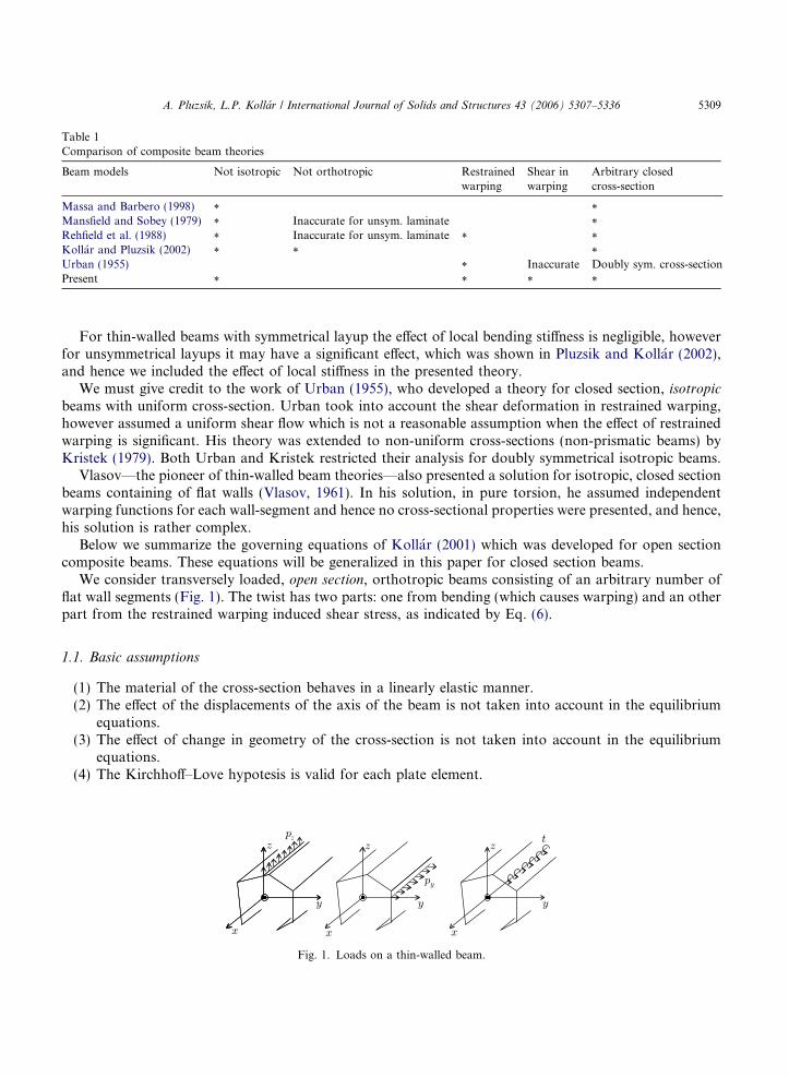
Table 1Comparison of composite beam theories
Beam models Not isotropic Not orthotropic Restrainedwarping
Shear inwarping
Arbitrary closedcross-section
Massa and Barbero (1998) * *Mansfield and Sobey (1979) * Inaccurate for unsym. laminate *Rehfield et al. (1988) * Inaccurate for unsym. laminate * *Kollar and Pluzsik (2002) * * *Urban (1955) * Inaccurate Doubly sym. cross-sectionPresent * * * *
A. Pluzsik, L.P. Kollar / International Journal of Solids and Structures 43 (2006) 5307–5336 5309
For thin-walled beams with symmetrical layup the effect of local bending stiffness is negligible, howeverfor unsymmetrical layups it may have a significant effect, which was shown in Pluzsik and Kollar (2002),and hence we included the effect of local stiffness in the presented theory.
We must give credit to the work of Urban (1955), who developed a theory for closed section, isotropic
beams with uniform cross-section. Urban took into account the shear deformation in restrained warping,however assumed a uniform shear flow which is not a reasonable assumption when the effect of restrainedwarping is significant. His theory was extended to non-uniform cross-sections (non-prismatic beams) byKristek (1979). Both Urban and Kristek restricted their analysis for doubly symmetrical isotropic beams.
Vlasov—the pioneer of thin-walled beam theories—also presented a solution for isotropic, closed sectionbeams containing of flat walls (Vlasov, 1961). In his solution, in pure torsion, he assumed independentwarping functions for each wall-segment and hence no cross-sectional properties were presented, and hence,his solution is rather complex.
Below we summarize the governing equations of Kollar (2001) which was developed for open sectioncomposite beams. These equations will be generalized in this paper for closed section beams.
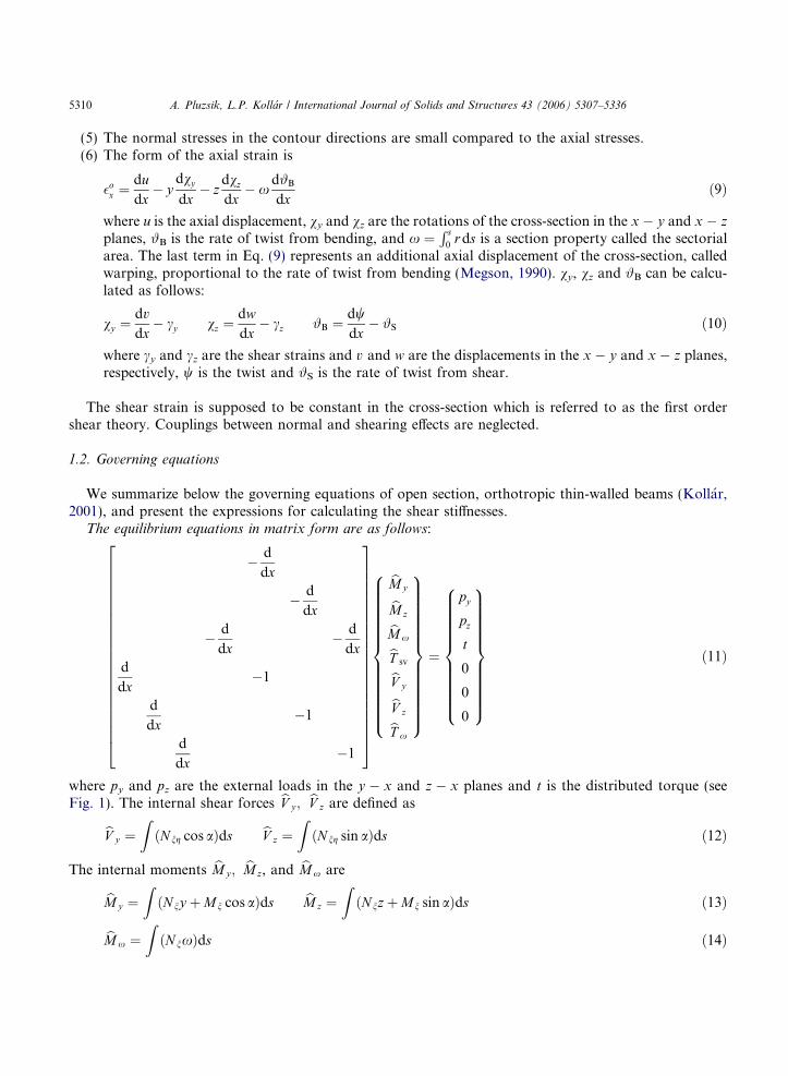
We consider transversely loaded, open section, orthotropic beams consisting of an arbitrary number offlat wall segments (Fig. 1). The twist has two parts: one from bending (which causes warping) and an otherpart from the restrained warping induced shear stress, as indicated by Eq. (6).
1.1. Basic assumptions
(1) The material of the cross-section behaves in a linearly elastic manner.(2) The effect of the displacements of the axis of the beam is not taken into account in the equilibrium
equations.(3) The effect of change in geometry of the cross-section is not taken into account in the equilibrium
equations.(4) The Kirchhoff–Love hypotesis is valid for each plate element.
Fig. 1. Loads on a thin-walled beam.
5310 A. Pluzsik, L.P. Kollar / International Journal of Solids and Structures 43 (2006) 5307–5336
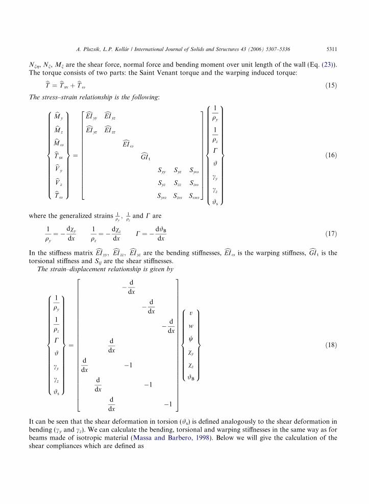
(5) The normal stresses in the contour directions are small compared to the axial stresses.(6) The form of the axial strain is
�ox ¼
dudx� y
dvy
dx� z
dvz
dx� x
d#B
dxð9Þ
where u is the axial displacement, vy and vz are the rotations of the cross-section in the x � y and x � z
planes, #B is the rate of twist from bending, and x ¼R s
0r ds is a section property called the sectorial
area. The last term in Eq. (9) represents an additional axial displacement of the cross-section, calledwarping, proportional to the rate of twist from bending (Megson, 1990). vy, vz and #B can be calcu-lated as follows:
vy ¼dvdx� cy vz ¼
dwdx� cz #B ¼
dwdx� #S ð10Þ
where cy and cz are the shear strains and v and w are the displacements in the x � y and x � z planes,respectively, w is the twist and #S is the rate of twist from shear.
The shear strain is supposed to be constant in the cross-section which is referred to as the first ordershear theory. Couplings between normal and shearing effects are neglected.
1.2. Governing equations
We summarize below the governing equations of open section, orthotropic thin-walled beams (Kollar,2001), and present the expressions for calculating the shear stiffnesses.
The equilibrium equations in matrix form are as follows:
� d
dx
� d
dx
� d
dx� d
dxd
dx�1
d
dx�1
d
dx�1
2666666666666666666664
3777777777777777777775
bM ybM zbM xbT svbV ybV zbT x
8>>>>>>>>>>>>><>>>>>>>>>>>>>:
9>>>>>>>>>>>>>=>>>>>>>>>>>>>;¼
py
pz
t
0
0
0
8>>>>>>>>>><>>>>>>>>>>:
9>>>>>>>>>>=>>>>>>>>>>;ð11Þ
where py and pz are the external loads in the y � x and z � x planes and t is the distributed torque (seeFig. 1). The internal shear forces bV y ; bV z are defined as
bV y ¼ZðN ng cos aÞds bV z ¼
ZðN ng sin aÞds ð12Þ
The internal moments bM y ; bM z, and bM x are
bM y ¼ZðN ny þMn cos aÞds bM z ¼
ZðN nzþMn sin aÞds ð13Þ
bM x ¼ZðN nxÞds ð14Þ
A. Pluzsik, L.P. Kollar / International Journal of Solids and Structures 43 (2006) 5307–5336 5311
Nng, Nn, Mn are the shear force, normal force and bending moment over unit length of the wall (Eq. (23)).The torque consists of two parts: the Saint Venant torque and the warping induced torque:
bT ¼ bT sv þ bT x ð15Þ The stress–strain relationship is the following:bM ybM zbM xbT svbV ybV zbT x
8>>>>>>>>>>>>>>>><>>>>>>>>>>>>>>>>:
9>>>>>>>>>>>>>>>>=>>>>>>>>>>>>>>>>;
¼
cEI yycEI yzcEI yzcEI zz cEI x cGI t
Syy Syz Syx
Syz Szz Szx
Syx Szx Sxx
266666666666666664
377777777777777775
1
qy
1
qz
C
#
cy
cz
#s
8>>>>>>>>>>>>>>>>>>><>>>>>>>>>>>>>>>>>>>:
9>>>>>>>>>>>>>>>>>>>=>>>>>>>>>>>>>>>>>>>;
ð16Þ
where the generalized strains 1qy; 1
qzand C are
1
qy¼ �
dvy
dx1
qz¼ � dvz
dxC ¼ � d#B
dxð17Þ
In the stiffness matrix cEI yy ; cEI zz; cEI yz are the bending stiffnesses, cEI x is the warping stiffness, cGI t is thetorsional stiffness and Sij are the shear stiffnesses.
The strain–displacement relationship is given by
1
qy
1
qz
C
#
cy
cz
#s
8>>>>>>>>>>>>>>>>>>><>>>>>>>>>>>>>>>>>>>:
9>>>>>>>>>>>>>>>>>>>=>>>>>>>>>>>>>>>>>>>;
¼
� d
dx
� d
dx
� d
dx
d
dx
d
dx�1
d
dx�1
d
dx�1
26666666666666666666666666664
37777777777777777777777777775
v
w
w
vy
vz
#B
8>>>>>>>>>>>><>>>>>>>>>>>>:
9>>>>>>>>>>>>=>>>>>>>>>>>>;ð18Þ
It can be seen that the shear deformation in torsion (#s) is defined analogously to the shear deformation inbending (cy and cz). We can calculate the bending, torsional and warping stiffnesses in the same way as forbeams made of isotropic material (Massa and Barbero, 1998). Below we will give the calculation of theshear compliances which are defined as
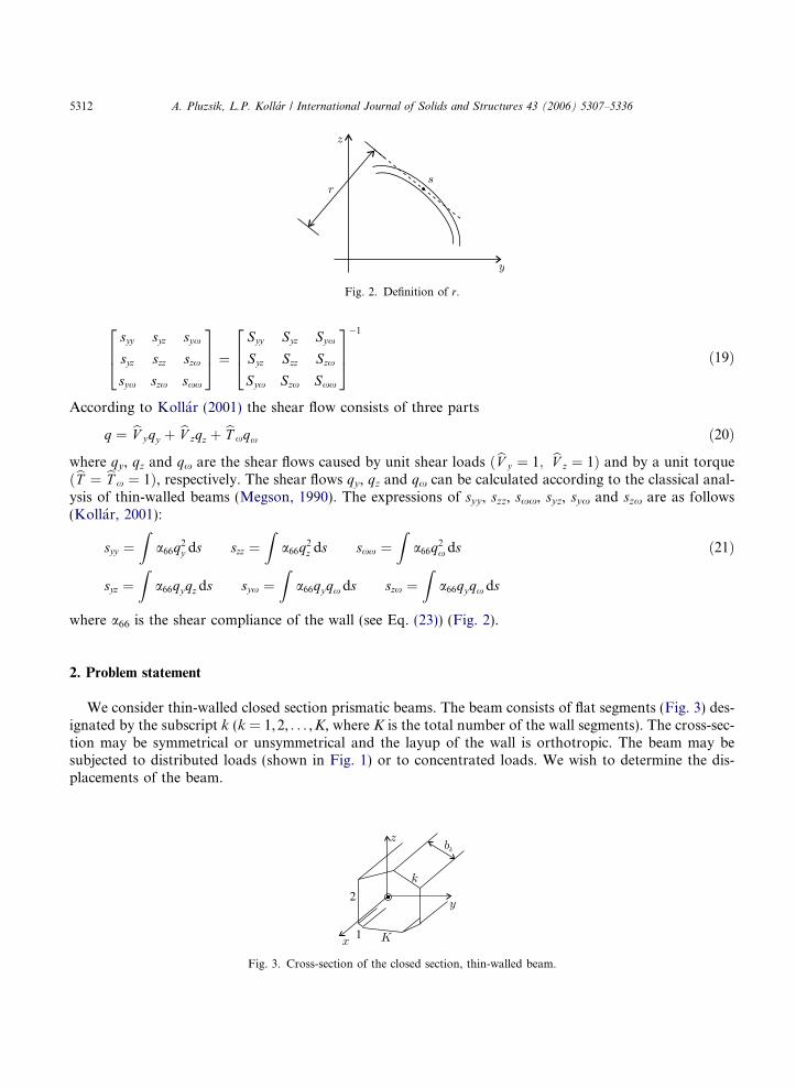
Fig. 2. Definition of r.
5312 A. Pluzsik, L.P. Kollar / International Journal of Solids and Structures 43 (2006) 5307–5336
syy syz syx
syz szz szx
syx szx sxx
264375 ¼ Syy Syz Syx
Syz Szz Szx
Syx Szx Sxx
264375�1
ð19Þ
According to Kollar (2001) the shear flow consists of three parts
q ¼ bV yqy þ bV zqz þ bT xqx ð20Þ
where qy, qz and qx are the shear flows caused by unit shear loads ðbV y ¼ 1; bV z ¼ 1Þ and by a unit torqueðbT ¼ bT x ¼ 1Þ, respectively. The shear flows qy, qz and qx can be calculated according to the classical anal-ysis of thin-walled beams (Megson, 1990). The expressions of syy, szz, sxx, syz, syx and szx are as follows(Kollar, 2001):
syy ¼Z
a66q2y ds szz ¼
Za66q2
z ds sxx ¼Z
a66q2x ds ð21Þ
syz ¼Z
a66qyqz ds syx ¼Z
a66qyqx ds szx ¼Z
a66qyqx ds
where a66 is the shear compliance of the wall (see Eq. (23)) (Fig. 2).
2. Problem statement
We consider thin-walled closed section prismatic beams. The beam consists of flat segments (Fig. 3) des-ignated by the subscript k (k = 1,2, . . . ,K, where K is the total number of the wall segments). The cross-sec-tion may be symmetrical or unsymmetrical and the layup of the wall is orthotropic. The beam may besubjected to distributed loads (shown in Fig. 1) or to concentrated loads. We wish to determine the dis-placements of the beam.
Fig. 3. Cross-section of the closed section, thin-walled beam.
A. Pluzsik, L.P. Kollar / International Journal of Solids and Structures 43 (2006) 5307–5336 5313
3. Governing equations
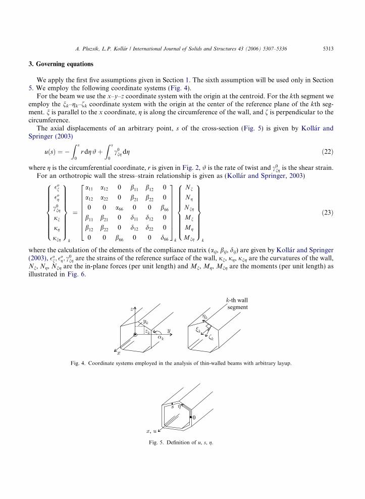
We apply the first five assumptions given in Section 1. The sixth assumption will be used only in Section5. We employ the following coordinate systems (Fig. 4).
For the beam we use the x–y–z coordinate system with the origin at the centroid. For the kth segment weemploy the nk–gk–fk coordinate system with the origin at the center of the reference plane of the kth seg-ment. n is parallel to the x coordinate, g is along the circumference of the wall, and f is perpendicular to thecircumference.
The axial displacements of an arbitrary point, s of the cross-section (Fig. 5) is given by Kollar andSpringer (2003)
uðsÞ ¼ �Z s
0
r dg#þZ s
0
c0ng dg ð22Þ
where g is the circumferential coordinate, r is given in Fig. 2, # is the rate of twist and c0ng is the shear strain.
For an orthotropic wall the stress–strain relationship is given as (Kollar and Springer, 2003)
�on
�og
c0ng
jn
jg
jng
8>>>>>>>><>>>>>>>>:
9>>>>>>>>=>>>>>>>>;k
¼
a11 a12 0 b11 b12 0
a12 a22 0 b21 b22 0
0 0 a66 0 0 b66
b11 b21 0 d11 d12 0
b12 b22 0 d12 d22 0
0 0 b66 0 0 d66
2666666664
3777777775k
N n
N g
N ng
Mn
Mg
Mng
8>>>>>>>><>>>>>>>>:
9>>>>>>>>=>>>>>>>>;k
ð23Þ
where the calculation of the elements of the compliance matrix (aij, bij, dij) are given by Kollar and Springer(2003), �o
n; �og; c
0ng are the strains of the reference surface of the wall, jn, jg, jng are the curvatures of the wall,
Nn, Ng, Nng are the in-plane forces (per unit length) and Mn, Mg, Mng are the moments (per unit length) asillustrated in Fig. 6.
Fig. 4. Coordinate systems employed in the analysis of thin-walled beams with arbitrary layup.
Fig. 5. Definition of u, s, g.
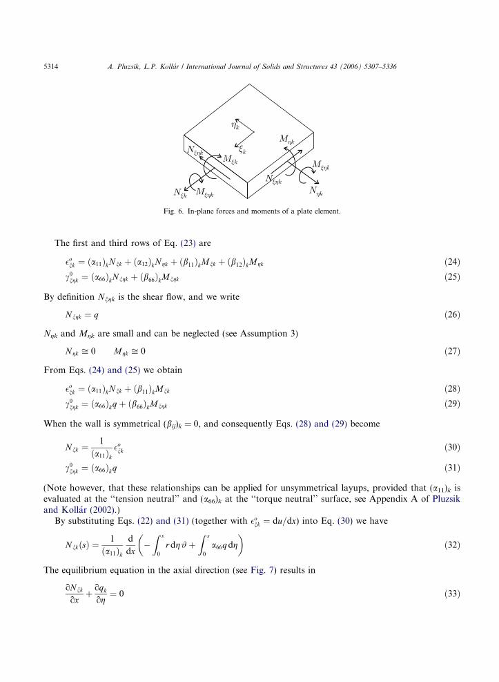
Fig. 6. In-plane forces and moments of a plate element.
5314 A. Pluzsik, L.P. Kollar / International Journal of Solids and Structures 43 (2006) 5307–5336
The first and third rows of Eq. (23) are
�onk ¼ ða11ÞkN nk þ ða12ÞkN gk þ ðb11ÞkMnk þ ðb12ÞkMgk ð24Þ
c0ngk ¼ ða66ÞkN ngk þ ðb66ÞkMngk ð25Þ
By definition Nngk is the shear flow, and we write
N ngk ¼ q ð26Þ
Ngk and Mgk are small and can be neglected (see Assumption 3)
N gk ffi 0 Mgk ffi 0 ð27Þ
From Eqs. (24) and (25) we obtain
�onk ¼ ða11ÞkN nk þ ðb11ÞkMnk ð28Þ
c0ngk ¼ ða66Þkqþ ðb66ÞkMngk ð29Þ
When the wall is symmetrical (bij)k = 0, and consequently Eqs. (28) and (29) become
N nk ¼1
ða11Þk�onk ð30Þ
c0ngk ¼ ða66Þkq ð31Þ
(Note however, that these relationships can be applied for unsymmetrical layups, provided that (a11)k isevaluated at the ‘‘tension neutral’’ and (a66)k at the ‘‘torque neutral’’ surface, see Appendix A of Pluzsikand Kollar (2002).)
By substituting Eqs. (22) and (31) (together with �onk ¼ du=dx) into Eq. (30) we have
N nkðsÞ ¼1
ða11Þkd
dx�Z s
0
r dg#þZ s
0
a66qdg
� �ð32Þ
The equilibrium equation in the axial direction (see Fig. 7) results in
oN nk
oxþ oqk
og¼ 0 ð33Þ
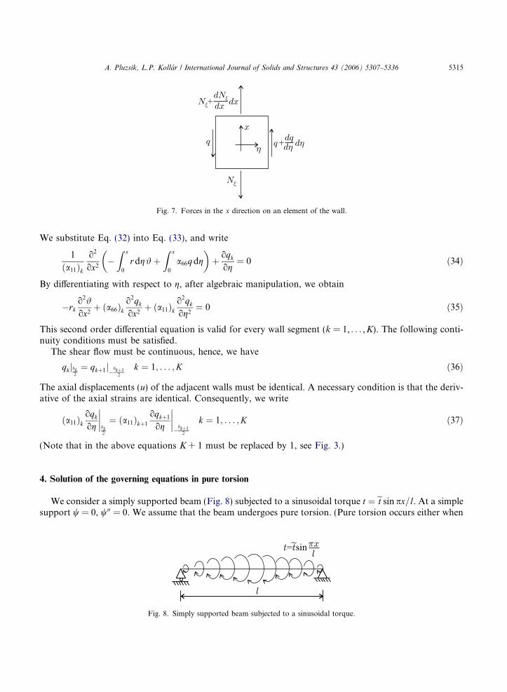
Fig. 7. Forces in the x direction on an element of the wall.
A. Pluzsik, L.P. Kollar / International Journal of Solids and Structures 43 (2006) 5307–5336 5315
We substitute Eq. (32) into Eq. (33), and write
1
ða11Þko2
ox2�Z s
0
r dg#þZ s
0
a66qdg
� �þ oqk
og¼ 0 ð34Þ
By differentiating with respect to g, after algebraic manipulation, we obtain
�rko2#
ox2þ ða66Þk
o2qk
ox2þ ða11Þk
o2qk
og2¼ 0 ð35Þ
This second order differential equation is valid for every wall segment (k = 1, . . . ,K). The following conti-nuity conditions must be satisfied.
The shear flow must be continuous, hence, we have
qkjbk2
¼ qkþ1j�bkþ12
k ¼ 1; . . . ;K ð36Þ
The axial displacements (u) of the adjacent walls must be identical. A necessary condition is that the deriv-ative of the axial strains are identical. Consequently, we write
ða11Þkoqk
og
����bk2
¼ ða11Þkþ1
oqkþ1
og
�����bkþ1
2
k ¼ 1; . . . ;K ð37Þ
(Note that in the above equations K + 1 must be replaced by 1, see Fig. 3.)
4. Solution of the governing equations in pure torsion
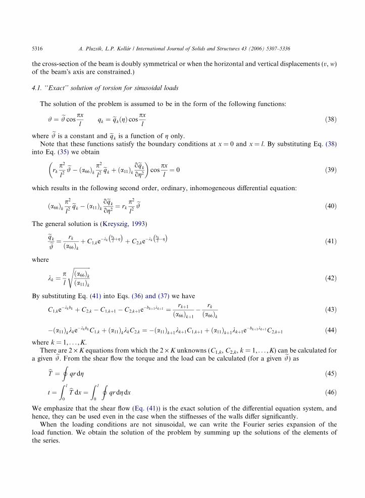
We consider a simply supported beam (Fig. 8) subjected to a sinusoidal torque t ¼ et sin px=l. At a simplesupport w = 0, w00 = 0. We assume that the beam undergoes pure torsion. (Pure torsion occurs either when
Fig. 8. Simply supported beam subjected to a sinusoidal torque.
5316 A. Pluzsik, L.P. Kollar / International Journal of Solids and Structures 43 (2006) 5307–5336
the cross-section of the beam is doubly symmetrical or when the horizontal and vertical displacements (v, w)of the beam�s axis are constrained.)
4.1. ‘‘Exact’’ solution of torsion for sinusoidal loads
The solution of the problem is assumed to be in the form of the following functions:
# ¼ e# cospxl
qk ¼ eqkðgÞ cospxl
ð38Þ
where e# is a constant and eqk is a function of g only.Note that these functions satisfy the boundary conditions at x = 0 and x = l. By substituting Eq. (38)
into Eq. (35) we obtain
rkp2
l2e# � ða66Þk
p2
l2eqk þ ða11Þk
oeqk
og2
� �cos
pxl¼ 0 ð39Þ
which results in the following second order, ordinary, inhomogeneous differential equation:
ða66Þkp2
l2eqk � ða11Þk
oeqk
og2¼ rk
p2
l2e# ð40Þ
The general solution is (Kreyszig, 1993)
eqke# ¼ rk
ða66Þkþ C1;ke�kk
bk2þg� �
þ C2;ke�kkbk2�g� �
ð41Þ
where
kk ¼pl
ffiffiffiffiffiffiffiffiffiffiffiffiða66Þkða11Þk
sð42Þ
By substituting Eq. (41) into Eqs. (36) and (37) we have
C1;ke�kk bk þ C2;k � C1;kþ1 � C2;kþ1e�bkþ1kkþ1 ¼ rkþ1
ða66Þkþ1
� rk
ða66Þkð43Þ
�ða11Þkkke�kk bk C1;k þ ða11ÞkkkC2;k ¼ �ða11Þkþ1kkþ1C1;kþ1 þ ða11Þkþ1kkþ1e�bkþ1kkþ1 C2;kþ1 ð44Þ
where k = 1, . . . ,K.There are 2 · K equations from which the 2 · K unknowns (C1,k, C2,k, k = 1, . . . ,K) can be calculated for
a given e#. From the shear flow the torque and the load can be calculated (for a given e#) as
bT ¼ I qr dg ð45Þ
t ¼Z l
0
bT dx ¼Z l
0
Iqr dgdx ð46Þ
We emphasize that the shear flow (Eq. (41)) is the exact solution of the differential equation system, andhence, they can be used even in the case when the stiffnesses of the walls differ significantly.
When the loading conditions are not sinusoidal, we can write the Fourier series expansion of theload function. We obtain the solution of the problem by summing up the solutions of the elements ofthe series.
A. Pluzsik, L.P. Kollar / International Journal of Solids and Structures 43 (2006) 5307–5336 5317
4.2. Solution by the Ritz method
In the following we derive an approximate solution of the above differential equations by the Ritz meth-od. The potential energy of the beam is
P ¼ 1
2
Z l
0
IN n�
on þ qc0
ng
� dgdx�
Z l
0
#t dx ð47Þ
where the first term is the strain energy and the second term is the work done by the external load.The axial force per unit length is (Eq. (33))
N n ¼ �Z l
0
oqog
dx ð48Þ
Eqs. (30), (31), (38), (48) and (47) result in
P ¼ 1
2
Z l
0
Ia11
l2
p2
oqog
� �2
þ a66q2
!dgdx�
Z l
0
#t dx ð49Þ
The shear flow is assumed to be in the form of
q ¼ eqðgÞ cospxl
ð50Þ
eqðgÞ ¼X2K
i¼1
Ci/iðgÞ ð51Þ
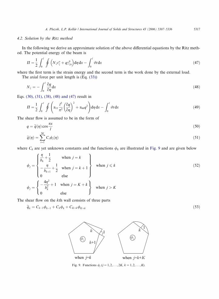
where Ck are yet unknown constants and the functions /k are illustrated in Fig. 9 and are given below
/j ¼
gbkþ 1
2when j ¼ k
� gbkþ1
þ 1
2when j ¼ k þ 1
0 else
8>>>><>>>>:
9>>>>=>>>>; when j 6 k ð52Þ
/j ¼� 4g2
b2k
þ 1 when j ¼ K þ k
0 else
8<:9=; when j > K
The shear flow on the kth wall consists of three parts
eqk ¼ Ck�1/k�1 þ Ck/k þ CKþk/Kþk ð53ÞFig. 9. Functions /j (j = 1,2, . . . , 2K, k = 1,2, . . . ,K).
5318 A. Pluzsik, L.P. Kollar / International Journal of Solids and Structures 43 (2006) 5307–5336
By substituting Eqs. (50) and (51) into Eq. (49) we obtain
P ¼ 1
2cT½F �c� cTf ð54Þ
where the kth element of the c and f vectors are
ck ¼ Ck fk ¼Z#/krk dg k ¼ 1; . . . ;K ð55Þ
and the ik element of matrix [F] is
F ik ¼XK
k¼1
Z bk=2
�bk=2
ða11Þkl2
p2
o/k
ogo/i
ogþ ða66Þk/k/i
� �dg ð56Þ
According to the principle of stationary potential energy, we have
P ¼ 1
2cT½F �c� cTf ¼ stationary! ð57Þ
The necessary condition for Eq. (57) is op/oCk = 0, which results in the following equation:
½F �c� f ¼ 0 ð58Þ
The unknown constants can be calculated asc ¼ ½F ��1f ð59Þ
When the constants are known, q can be calculated by Eq. (50). From q the torque load can be calculatedby Eq. (46).
5. Beam theory
All the six assumptions of Section 1 are valid, the last one is reiterated here.The axial strain is (Eq. (9))
�ox ¼
dudx� y
dvy
dx� z
dvz
dx� x
d#B
dxð60Þ
where vy, vz and #B are given by Eq. (10).
5.1. Governing equations in pure torsion
For convenience we separate the shear flow q as
q ¼ q0 þ qx ð61Þ
where q0 is uniform around the circumference (Fig. 10).These shear flows result in the following torques:
bT sv ¼I
q0r dg bT x ¼I
qxr dg ð62Þ
and the total torque is
bT ¼ bT sv þ bT x ð63Þ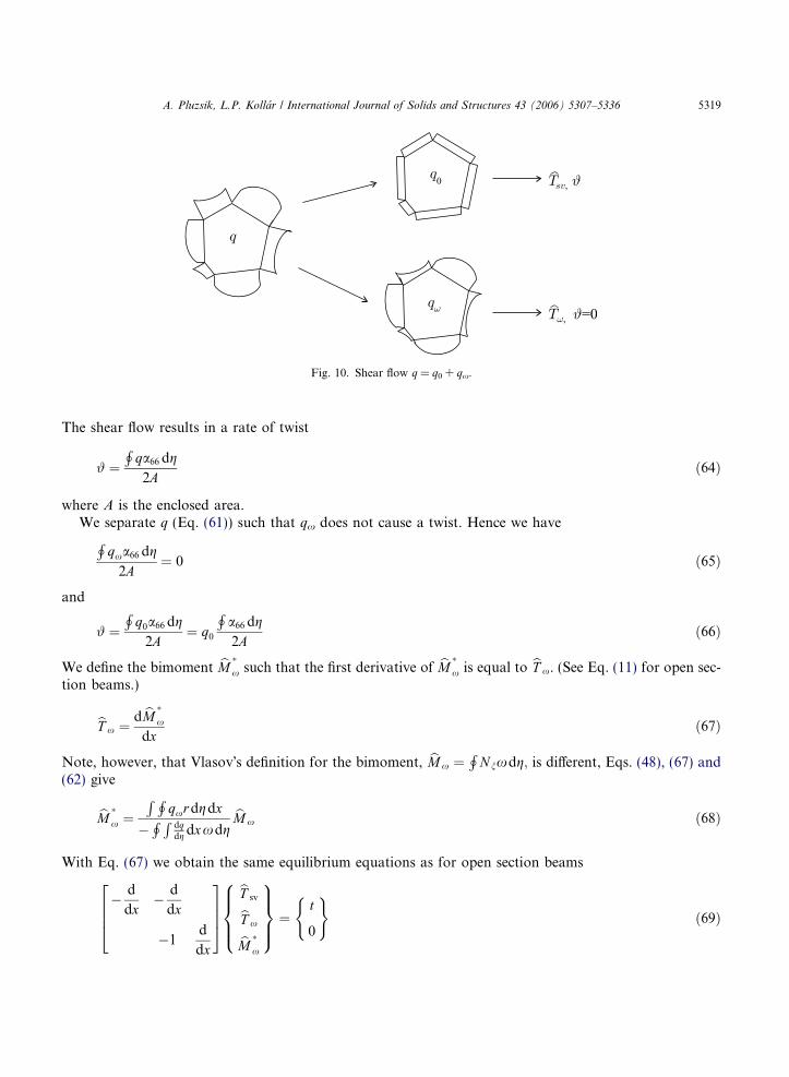
Fig. 10. Shear flow q = q0 + qx.
A. Pluzsik, L.P. Kollar / International Journal of Solids and Structures 43 (2006) 5307–5336 5319
The shear flow results in a rate of twist
# ¼H
qa66 dg2A
ð64Þ
where A is the enclosed area.We separate q (Eq. (61)) such that qx does not cause a twist. Hence we have
Hqxa66 dg
2A¼ 0 ð65Þ
and
# ¼H
q0a66 dg2A
¼ q0
Ha66 dg2A
ð66Þ
We define the bimoment bM �x such that the first derivative of bM �
x is equal to bT x. (See Eq. (11) for open sec-tion beams.)
bT x ¼d bM �
x
dxð67Þ
Note, however, that Vlasov�s definition for the bimoment, bM x ¼H
N nxdg; is different, Eqs. (48), (67) and(62) give
bM �x ¼
R Hqxr dgdx
�H R
dqdg dxxdg
bM x ð68Þ
With Eq. (67) we obtain the same equilibrium equations as for open section beams
� d
dx� d
dx
�1d
dx
26643775
bT svbT xbM �x
8>><>>:9>>=>>; ¼
t
0
( )ð69Þ
5320 A. Pluzsik, L.P. Kollar / International Journal of Solids and Structures 43 (2006) 5307–5336
Similarly, as for open section beams, we assume that the rate of twist consists of two terms, # = #S + #B
(Eq. (6)) and write the strain–displacement relationship as (Eq. (18))
#
#S
C
8<:9=; ¼
d
dxd
dx�1
� d
dx
2666664
3777775w#B
�ð70Þ
and assume that these generalized strains are related to the internal forces by
bT svbT xbM �x8<:9=; ¼
bGI t
Sxx cEI x
24 35 #
#S
C
8<:9=; ð71Þ
where bGI t, Sxx and cEI x are yet unknown stiffnesses. In the following section we will determine expressionsfor the stiffnesses to obtain an acceptable description for the beam with the above governing equations.
5.2. Replacement stiffnesses in pure torsion
To determine the stiffnesses bGI t, Sxx and cEI x of the beam, we will make use of the derived solution forthe case of beams subjected to a sinusoidal load (Sections 4.1, 4.2, Fig. 8).
The strain energy of the beam is
U ¼ 1
2
Z l
0
Za11N n|fflffl{zfflffl}
�on
N n þ a66q|{z}c0ng
q
0BB@1CCAdg
0BB@1CCAdx ð72Þ
We introduced the internal forces, generalized strains and the stiffnesses of the beam in the previous section.By using these definitions the strain energy can be written as
U ¼ 1
2
Z l
0
bT sv#þ bT x#s þ bM �xC
� dx ¼ 1
2
Z l
0
bT 2
svbGI t
þbT 2
x
SxxþbM �2
xcEI x
!dx ð73Þ
We recall (Eq. (38)) that for a sinusoidal load q and # are trigonometrical functions, and hence, bT sv; bT x
and bM �x are also trigonometrical functions and the integration with respect to x can be performed. From
Eqs. (72) and (73), together with Eq. (48) we obtain
U ¼ 1
2
lp
Ia11
l2
p2
oqog
� �2
þ a66q2 dg ð74Þ
and
U ¼ 1
2
lp
bT 2
svbGI t
þbT 2
x
SxxþbM �2
xcEI x
!ð75Þ
We introduce q = q0 + qx (Eq. (61)) into Eq. (74) and obtain
U ¼ 1
2
lp
Za66q2
0 dgþZ
a66q2x dgþ l2
p2
Za11
oqog
� �2
dgþ 2q0
Zqxa66 dg|fflfflfflfflfflfflffl{zfflfflfflfflfflfflffl}
0
0BB@1CCA ð76Þ
As a consequence of Eq. (65) the last term in Eq. (76) is zero.
A. Pluzsik, L.P. Kollar / International Journal of Solids and Structures 43 (2006) 5307–5336 5321
Introducing Eqs. (62) and (67) into Eq. (75) we obtain
U ¼ 1
2
lpðH
q0r dsÞ2bGI t
þ ðH
qxr dsÞ2
SxxþðlpH
qxr dsÞ2cEI x
!ð77Þ
By comparing Eqs. (76) and (77) we have
bGI t ¼ðH
q0r dsÞ2Ra66q2
0 dgð78Þ
Sxx ¼ðH
qxr dsÞ2Ra66q2
x dgð79Þ
cEI x ¼ðH
qxr dsÞ2Ra11ðo
2qog2 Þ2 dg
ð80Þ
q0 is uniform around the circumference, hence Eq. (78) becomes
bGI t ¼ðH
r dsÞ2Ra66 dg
¼ 4A2Ra66 dg
ð81Þ
To determine Sxx and cEI x the distribution of qx must be known. In Sections 4.1 and 4.2 we determined qx,and obtained that qx depends on the length l, and as a consequence, Sxx and cEI x also depend on l. Toderive stiffnesses which are independent of the length l we will assume that l/bk� 1, where bk is the widthof the kth wall segment.
To calculate the stiffnesses we may either use the ‘‘exact’’ solution (see Eq. (41)) or the approximate solu-tion obtained via the Ritz method (see Eq. (50)). To obtain simpler results the approximate solution will beused. First the expressions for a doubly symmetrical box beam is derived then a general cross-section under-going pure torsion will be considered.
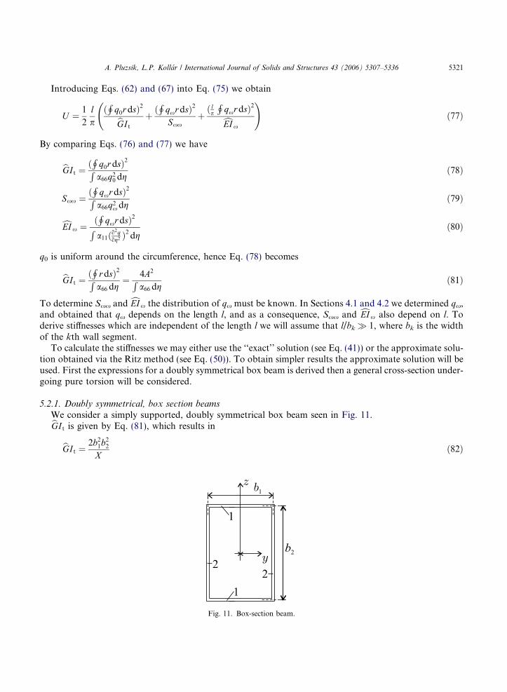
5.2.1. Doubly symmetrical, box section beams
We consider a simply supported, doubly symmetrical box beam seen in Fig. 11.bGI t is given by Eq. (81), which results in
bGI t ¼2b2
1b22
Xð82Þ
Fig. 11. Box-section beam.
5322 A. Pluzsik, L.P. Kollar / International Journal of Solids and Structures 43 (2006) 5307–5336
where
X ¼ ða66Þ1b1 þ ða66Þ2b2 ð83Þ
The beam is subjected to a torque load t ¼ et sin px=l (Fig. 8). Under the applied load the beam undergoes arate of twist # ¼ e# cos px=l, where e# is a yet unknown constant.
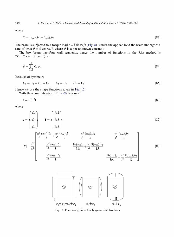
The box beam has four wall segments, hence the number of functions in the Ritz method is2K = 2 · 4 = 8, and eq is
eq ¼X8
k¼1
Ck/k ð84Þ
Because of symmetry
C1 ¼ C2 ¼ C3 ¼ C4 C5 ¼ C7 C6 ¼ C8 ð85Þ
Hence we use the shape functions given in Fig. 12.With these simplifications Eq. (59) becomes
c ¼ ½F ��1f ð86Þ
where
c ¼
C1
C5
C6
8>>><>>>:9>>>=>>>; f ¼
A=2
A=3
A=3
8>>><>>>:9>>>=>>>; ð87Þ
½F � ¼ l2
p2
p2
l2
ða66Þ1b1
2þ p2
l2
ða66Þ2b2
2
p2
l2
ða66Þ1b1
3
p2
l2
ða66Þ2b2
3
p2
l2
ða66Þ1b1
3
16ða11Þ13b1
þ p2
l2
8ða66Þ1b1
15
p2
l2
ða66Þ2b2
3
16ða11Þ23b2
þ p2
l2
8ða66Þ2b2
15
26666666664
37777777775ð88Þ
Fig. 12. Functions /k for a doubly symmetrical box beam.
A. Pluzsik, L.P. Kollar / International Journal of Solids and Structures 43 (2006) 5307–5336 5323
Solution of Eq. (86) results in
C1 ¼ e# p2
l2A2
1
2�
13
ða66Þ1b1
3A p2
l2
A 16ða11Þ13b1þ A p2
l2
8ða66Þ1b1
15
�13
ða66Þ2b2
3A p2
l2
A 16ða11Þ23b2þ A p2
l2
8ða66Þ2b2
15
ða66Þ1b1
2A
p2
l2þ ða66Þ2b2
2A
p2
l2� 2
ða66Þ1b1
3A p2
l2
� 2
A 16ða11Þ13b2þ A p2
l2
8ða66Þ1b1
15
� 2
ða66Þ2b2
3A p2
l2
� 2
A 16ða11Þ23b2þ A p2
l2
8ða66Þ21b2
15
C5 ¼ e# p2
l2
A2
3� 2ða66Þ1b1
3A
p2
l2C1
A16ða11Þ1
3b1
þ Ap2
l2
8ða66Þ1b1
15
C6 ¼ e# p2
l2
A2
3� 2ða66Þ2b2
3A
p2
l2C1
A16ða11Þ2
3b2
þ Ap2
l2
8ða66Þ2b2
15
ð89Þ
The Taylor series expression of these expressions with respect toffiffiffiAp
p=l are as follows:
C1 ¼ e# AXþ p2
l2
2AY
3X 2� ða66Þ1b1
16ða11Þ1b1
þ ða66Þ2b2
16ða11Þ2b2
0BB@1CCAþ p4
l4� � �|fflfflfflffl{zfflfflfflffl}
neglected
8>><>>:9>>=>>;
C5 ¼ e# p2
l2
AY16ða11Þ1
b1
Xþ p4
l4� � �|fflfflfflffl{zfflfflfflffl}
neglected
8>><>>:9>>=>>;
C6 ¼ e# � p2
l2
AY16ða11Þ2
b2
Xþ p4
l4� � �|fflfflfflffl{zfflfflfflffl}
neglected
8>><>>:9>>=>>;
ð90Þ
where
Y ¼ ða66Þ2b2 � ða66Þ1b1 ð91Þ
and X is defined in Eq. (83). In these expressions we neglect the terms containing ðffiffiffiAp
p=lÞi, when i P 4.The rate of twist can be calculated by Eq. (66), which is
# ¼ e# cospxl¼ eq0 cos
pxl
Ha66 dg
2Að92Þ
Eq. (92) gives the uniform shear flow
eq0 ¼ e# 2AHa66 dg
ð93Þ
For the box beam » a66 dg = 2(a66)1b1 + 2(a66)2b2 = 2X and hence
eq0 ¼ e# AX
ð94Þ
5324 A. Pluzsik, L.P. Kollar / International Journal of Solids and Structures 43 (2006) 5307–5336
The shear flow qx is calculated as
qx ¼ q� q0 ð95Þ
Eqs. (84) and (95) give eqx ¼ ðC1 � eq0Þ/1 þ C5/2 þ C6/3 ð96Þ By introducing Eq. (96) into (79) and (80) we obtainSxx ¼A2
2X 2
ðn2 � n1Þ2
n1n2ð1þ jÞcEI x ¼
A2
24ðn2 � n1Þ2Z ð97Þ
where
Z ¼ b1
ða11Þ1þ b2
ða11Þ2
n1 ¼b1ða66Þ1
Xn2 ¼ 1� n1 ð98Þ
j ¼ n1g21 þ n2g2
2
5n1n2ðg1 þ g2Þ2
ð99Þ
g1 ¼b1=ða11Þ1
Zg2 ¼ 1� g1 ð100Þ
(X is given by Eq. (83).)
5.2.2. General cross-section beams
We consider a thin-walled closed section beam consisting of K plane wall segments (Fig. 3). The torsionalstiffness cGI t is given by Eq. (81) which results in
cGI t ¼4A2PK
k¼1ða66Þkbk
ð101Þ
where bk and (a66)k are the width and the shear compliance of the kth wall segment, and A is the enclosedarea.
The beam is subjected to a torque load t ¼ et sin px=l and the beam undergoes a rate of twist# ¼ e# cos px=l. The shear flow of the beam is approximated by (see Eq. (50))
eq ¼X2K
k¼1
Ck/k ð102Þ
where /k is illustrated in Fig. 9, and Ck are yet unknown constants. The equation to determine these con-stants were derived in Section 4.2, and is reiterated below
½F �c ¼ f ð103Þ
wherec ¼
C1
C2
..
.
C2K
8>>>><>>>>:
9>>>>=>>>>; f ¼
f1
f2
..
.
f2K
8>>>><>>>>:
9>>>>=>>>>; ð104Þ
A. Pluzsik, L.P. Kollar / International Journal of Solids and Structures 43 (2006) 5307–5336 5325
and [F] is
TableElemen
½F � ¼ l2
p2
½A1�½A2�
�|fflfflfflfflfflfflfflfflffl{zfflfflfflfflfflfflfflfflffl}
½A�
þ½B1� ½B2�½B2�T ½B3�
�|fflfflfflfflfflfflfflfflfflffl{zfflfflfflfflfflfflfflfflfflffl}
½B�
ð105Þ
where the elements of vector f and matrices [A1], [A2], [B1], [B2] and [B3] are given in Table 2.Solution of Eq. (103) is assumed to be in the form of
c ¼ ec þ p2
l2eec þ p4
l4
eeec þ � � � ð106Þ
By introducing Eqs. (105) and (106) into Eq. (103) we obtain
l2
p2½A� þ ½B�
� � ec þ p2
l2eec þ p4
l4
eeec þ � � �� �¼ f ð107Þ
which gives
½A�ec þ p2
l2ð½B�ec þ ½A�eecÞþ p4
l4� � �|fflfflfflffl{zfflfflfflffl}
neglected
¼ p2
l2f ð108Þ
In this equation we neglect the terms pi/li when i P 4. In order to obtain the ‘‘best’’ solution we make equalthe multipliers of pi/li in the two sides of Eq. (108), and write
½A�ec ¼ 0 ð109Þ½B�ec þ ½A�eec ¼ f ð110Þ
Matrix [A] is singular. The non-trivial solution of (Eq. (109)) is
ec1 ¼ ec2 ¼ � � � ¼ ecK ¼ const ecKþ1 ¼ ecKþ2 ¼ � � � ¼ ec2K ¼ 0 ð111Þ The choice of the constant is not unambiguous. Here we propose the constant value to be equal to the shearflow resulting in an infinitely long beam. Hence we write (Eq. (93)):2ts of matrices [A1], [A2], [B1], [B2], [B3] and vector f
[A1]
ða11Þjbjþ ða11Þi
bii ¼ j
�ða11Þibi
when i ¼ jþ 1
�ða11Þj
bji ¼ j� 1
0 else
8>>>>>>>><>>>>>>>>:[B1]
ða66Þibi
3þða66Þjbj
3i ¼ j
ða66Þibi
6when i ¼ jþ 1
ða66Þjbj
6i ¼ j� 1
0 else
8>>>>>>><>>>>>>>:[A2]
16ða11Þi3bi
when i ¼ j
0 else
8<: [B2]
ða66Þibi
3i ¼ j
ða66Þjbj
3when i ¼ j� 1
0 else
8>>><>>>:
f
bkrk
2when k 6 K
2bkrk3 k P K
8<: [B3]8ða66Þibi
15when i ¼ j
0 else
(
5326 A. Pluzsik, L.P. Kollar / International Journal of Solids and Structures 43 (2006) 5307–5336
ec1 ¼ ec2 ¼ � � � ¼ ecK ¼ eq0 ¼ e# 2APKk¼1ða66Þkbk
ð112Þ
Eq. (110) gives 2K equations to determine eec .
½A�eec ¼ f � ½B�ec ð113Þ
[A] is singular and, consequently, the elements of eec cannot be determined unambiguously from Eq. (113)only. However we have an additional condition which is discussed below.We may observe (see Eqs. (111) and (112)) that
eq0 ¼X2K
k¼1
eCk/k ¼XK
k¼1
eCk/k ð114Þ
and, consequently (see Eqs. (61), (101) and (106))
eqx ¼p2
l2
X2K
k¼1
eeC k/k ð115Þ
We now make use of Eq. (65), which can be given in the following form:
XK
k¼1
eeC kða66Þkbk
2þða66Þkþ1bkþ1
2
� �þXK
k¼1
eeC kþK2ða66Þkbk
3¼ 0 ð116Þ
The elements ofeeC k are determined from the following 2K equations: The 2nd through 2Kth equations of
Eq. (113)
X2K
j¼1
AjkeeC k ¼ fk � eq0
XK
j¼1
Bjk k ¼ 2; 3; . . . ; 2K ð117Þ
and from Eq. (116). We substituteeeC k into Eq. (115) and then into Eqs. (79) and (80) which results in
Sxx ¼
PKk¼1rkbk
eeC k�1þeeC k
2þ 2
3
eeC Kþk
! !2
PKk¼1ða66Þkbk
eeC 2
k�1þeeC 2
kþeeC k�1
eeC k
3þ 8
15
eeC 2
Kþk þ 23
eeC KþkeeC k�1 þ eeC k
� 0@ 1A
cEI x ¼
PKk¼1rkbk
eeC k�1þeeC k
2þ 2
3
eeC Kþk
! !2
PKk¼1
ða11Þkbk
� eeC k�1 þ eeC k
� 2
þ 163
eeC 2
Kþk
� � ð118Þ
Note that we derived explicit expressions for cGI t, Sxx and cEI x which are independent of the beam�slength.
5.3. Bending–torsion coupling—unsymmetrical beams
In the previous section we considered beams undergoing pure torsion.As a rule beams undergo lateral and torsional deformations simultaneously. By combining Eq. (16) and
Eq. (71) we write
A. Pluzsik, L.P. Kollar / International Journal of Solids and Structures 43 (2006) 5307–5336 5327
cy
cz
#
#s
8>>>>><>>>>>:
9>>>>>=>>>>>;¼
syy syz sy0 syx
syz szz sz0 szx
sy0 sz0 s00 s0x
syx szx sx0 sxx
2666664
3777775bV ybV zbT svbT x
8>>>>>><>>>>>>:
9>>>>>>=>>>>>>;ð119Þ
where sij are the shear compliances. To determine the shear compliances we write the shear flow as
q ¼ qy þ qz þ qT ð120Þ
where qy, qz, qT are the shear flows from the shear forces bV y and bV z and from the torque bT , respectively.The shear flow from the torque is separated as (Eq. (61)):
qT ¼ q0 þ qx ð121Þ
Hence we have
bV y ¼Z
qy dg
bV z ¼Z
qz dg
bT sv ¼Z
rq0 dg
bT x ¼Z
rqx dg
ð122Þ
The compliances are determined similarly as for pure torsion. The strain energy of the beam is
U ¼ UN þ Uq ¼1
2
Za11
l2
p2
o2qog2
� �2
dgþ 1
2
Za66q2 dg ð123Þ
With the internal forces in Eq. (119) we write
Uq ¼1
2bV 2
y syy þ1
2bV 2
z szz þ1
2bT 2
svs00 þ1
2bT 2
xsxx þ bV ybV zsyz þ bV y
bT svsy0 þ bV zbT svsz0 þ bV y
bT xsyx
þ bV zbT xszx þ bT sv
bT xsx0 ð124Þ
By introducing Eqs. (120 and 121) into the second part of Eq. (123) we have
Uq ¼1
2
Za66 q2
y þ q2z þ q2
0 þ q2x þ 2qyqz þ 2qyq0 þ 2qyqx þ 2qzq0 þ 2qzqx þ 2q0qx
� dg ð125Þ
By comparing Eq. (124) and (125) we obtain
sij ¼R
a66qiqj dgRqiðrÞdg
RqjðrÞdg
i; j ¼ y; z; 0;w ð126Þ
The shear flows q0 and qx can be calculated according to the previous section, while qy and qz according toclassical textbooks.
Eq. (65) results in
sx0 ¼ 0 ð127Þ
5328 A. Pluzsik, L.P. Kollar / International Journal of Solids and Structures 43 (2006) 5307–5336
6. Verification
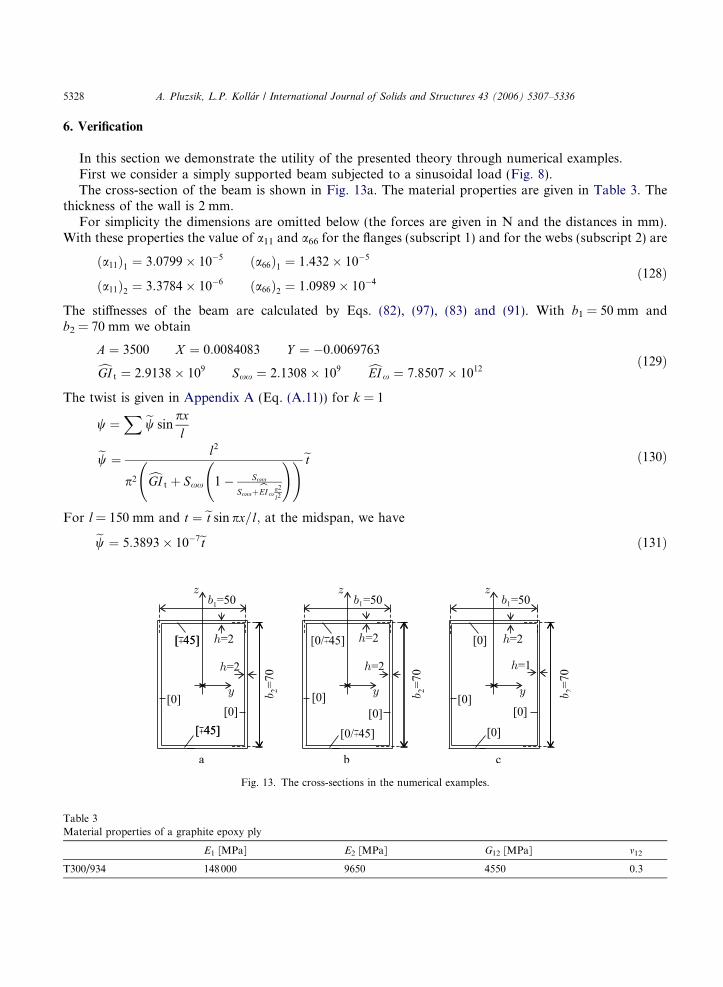
In this section we demonstrate the utility of the presented theory through numerical examples.First we consider a simply supported beam subjected to a sinusoidal load (Fig. 8).The cross-section of the beam is shown in Fig. 13a. The material properties are given in Table 3. The
thickness of the wall is 2 mm.For simplicity the dimensions are omitted below (the forces are given in N and the distances in mm).
With these properties the value of a11 and a66 for the flanges (subscript 1) and for the webs (subscript 2) are
TableMater
T300/9
ða11Þ1 ¼ 3:0799� 10�5 ða66Þ1 ¼ 1:432� 10�5
ða11Þ2 ¼ 3:3784� 10�6 ða66Þ2 ¼ 1:0989� 10�4ð128Þ
The stiffnesses of the beam are calculated by Eqs. (82), (97), (83) and (91). With b1 = 50 mm andb2 = 70 mm we obtain
A ¼ 3500 X ¼ 0:0084083 Y ¼ �0:0069763cGI t ¼ 2:9138� 109 Sxx ¼ 2:1308� 109 cEI x ¼ 7:8507� 1012ð129Þ
The twist is given in Appendix A (Eq. (A.11)) for k = 1
w ¼Xew sin
pxlew ¼ l2
p2 cGI t þ Sxx 1� Sxx
SxxþbEI xp2
l2
! !et ð130Þ
For l = 150 mm and t ¼ et sin px=l; at the midspan, we have
ew ¼ 5:3893� 10�7et ð131ÞFig. 13. The cross-sections in the numerical examples.
3ial properties of a graphite epoxy ply
E1 [MPa] E2 [MPa] G12 [MPa] m12
34 148000 9650 4550 0.3
A. Pluzsik, L.P. Kollar / International Journal of Solids and Structures 43 (2006) 5307–5336 5329
We calculated the twist of the middle section also by solving the differential equation system of the walls(Section 4.1, ‘‘accurate solution’’), and we obtained
Fig.
ew ¼ 5:3352� 10�7et ð132Þ
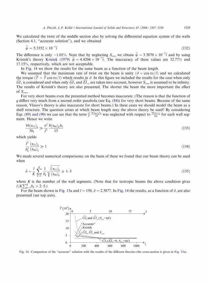
The difference is only �1.01%. Note that by neglecting Sxx we obtain ew ¼ 3:5870� 10�7et and by usingKristek�s theory Kristek (1979) ew ¼ 4:4204� 10�7et. The inaccuracy of these values are 32.77% and17.15%, respectively, which are not acceptable.In Fig. 14 we show the results for the same beam as a function of the beam length.We assumed that the maximum rate of twist on the beam is unity ð# ¼ cos px=lÞ and we calculated
the torque ðbT ¼ eT cos px=lÞ which results in #. In this figure we included the results for the case when onlycGI t is considered and when only cGI t and cEI x are taken into account, however Sxx is assumed to be infinity.The results of Kristek�s theory are also presented. The shorter the beam the more important the effectof Sxx.
For very short beams even the presented method becomes inaccurate. (The reason is that the function ofq differs very much from a second order parabola (see Eq. (84)) for very short beams. Because of the samereason, Vlasov�s theory is also inaccurate for short beams.) In these cases we should model the beam as ashell structure. The question arises at which beam length may the above theory be used? By consideringEqs. (89) and (90) we can see that the term p2
l2
8ða66Þk bk
15was neglected with respect to 16ða11Þk
3bkfor each wall seg-
ment. Hence we write
16ða11Þk3bk
� p2
l2
8ða66Þkbk
15ð133Þ
which yields
l2
b2k
ða11Þkða66Þk
� 1 ð134Þ
We made several numerical comparisons; on the basis of these we found that our beam theory can be usedwhen
d ¼ lK
XK
k¼1
1
bk
ffiffiffiffiffiffiffiffiffiffiffiffiða11Þkða66Þk
sP 1–3 ð135Þ
where K is the number of the wall segments. (Note that for isotropic beams the above condition givesl=K
PKk¼1bk > 2–5.)
For the beam shown in Fig. 13a and l = 150, d = 2.3877. In Fig. 14 the results, as a function of d, are alsopresented (see top axis).
14. Comparison of the ‘‘accurate’’ solution with the results of the different theories (the cross-section is given in Fig. 13a).
5330 A. Pluzsik, L.P. Kollar / International Journal of Solids and Structures 43 (2006) 5307–5336
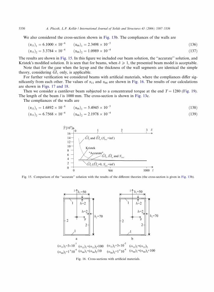
We also considered the cross-section shown in Fig. 13b. The compliances of the walls are
Fig.
ða11Þ1 ¼ 6:1000� 10�6 ða66Þ1 ¼ 2:3498� 10�5 ð136Þða11Þ2 ¼ 3:3784� 10�6 ða66Þ2 ¼ 1:0989� 10�4 ð137Þ
The results are shown in Fig. 15. In this figure we included our beam solution, the ‘‘accurate’’ solution, andKristek�s modified solution. It is seen that for beams, when d P 1, the presented beam model is acceptable.
Note that for the case when the layup and the thickness of the wall segments are identical the simpletheory, considering cGI t only, is applicable.
For further verification we considered beams with artificial materials, where the compliances differ sig-nificantly from each other. The values of a11 and a66 are shown in Fig. 16. The results of our calculationsare shown in Figs. 17 and 18.
Then we consider a cantilever beam subjected to a concentrated torque at the end T = 1280 (Fig. 19).The length of the beam l is 1000 mm. The cross-section is shown in Fig. 13c.
The compliances of the walls are
ða11Þ1 ¼ 1:6892� 10�6 ða66Þ1 ¼ 5:4945� 10�5 ð138Þða11Þ2 ¼ 6:7568� 10�6 ða66Þ2 ¼ 2:1978� 10�4 ð139Þ
15. Comparison of the ‘‘accurate’’ solution with the results of the different theories (the cross-section is given in Fig. 13b).
Fig. 16. Cross-sections with artificial materials.

Fig. 18. Comparison of the ‘‘accurate’’ solution with the results of the different theories (the cross-section is given in Fig. 16b).
Fig. 19. Cantilever beam subjected to a torque at the end.
Fig. 17. Comparison of the ‘‘accurate’’ solution with the results of the different theories (the cross-section is given in Fig. 16a).
A. Pluzsik, L.P. Kollar / International Journal of Solids and Structures 43 (2006) 5307–5336 5331
The stiffnesses of the beam cGI t, Sxx and cEI x are given by Eqs. (82) and (97):
cGI t ¼ 1:3512� 109 Sxx ¼ 1:0479� 108 cEI x ¼ 9:9078� 1012 ð140Þ The function of the twist is given by Eq. (B.7) in Appendix B:w ¼ C1 þ C2xþ C3ekðx�LÞ þ C4e�kx ð141Þ
where k = 0.0077, C1 = �0.5361 · 10�4, C2 = 0.0095 · 10�4, C3 = 0 and C4 = 0.5361 · 10�4.The rate of twist (i.e. the first derivative of the twist) is
# ¼ C2 þ C3kekðx�LÞ � C4ke�kx ¼ 10�4 � ð0:0095� 0:0041� e�0:0077xÞ ð142Þ
The rate of twist was also calculated by the ANSYS FE program. The results are compared to each other inFig. 20. It can be seen that the analytical and numerical calculations agree well.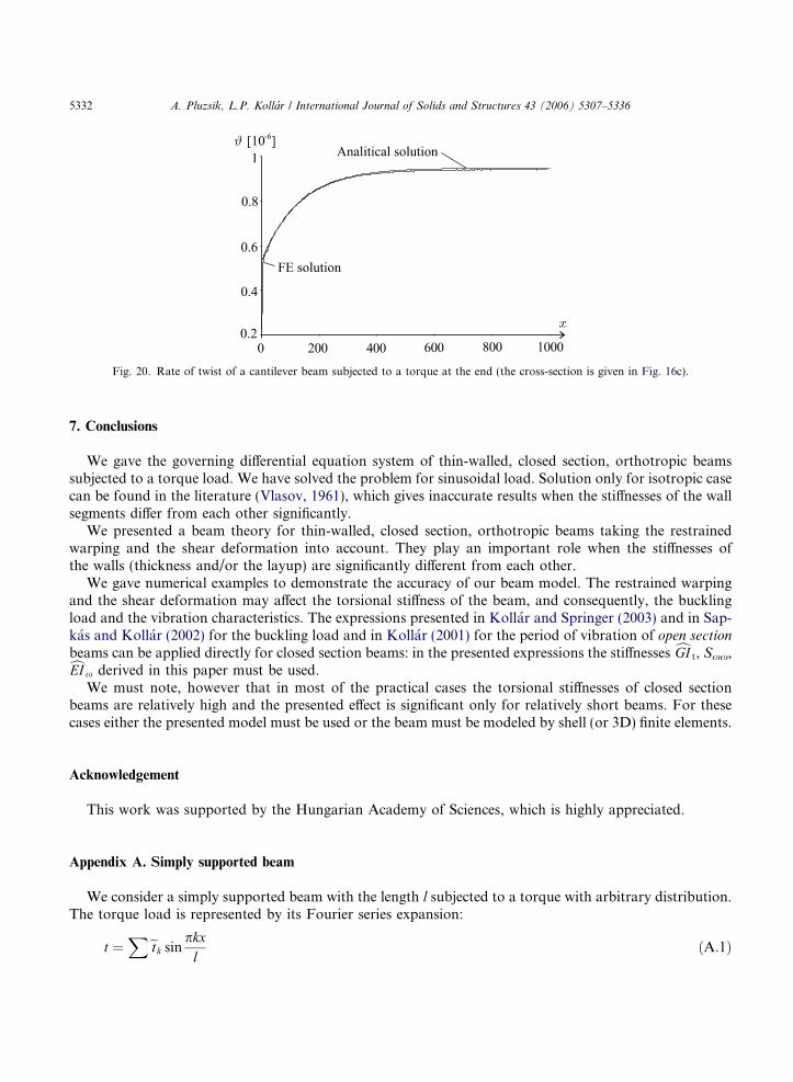
Fig. 20. Rate of twist of a cantilever beam subjected to a torque at the end (the cross-section is given in Fig. 16c).
5332 A. Pluzsik, L.P. Kollar / International Journal of Solids and Structures 43 (2006) 5307–5336
7. Conclusions
We gave the governing differential equation system of thin-walled, closed section, orthotropic beamssubjected to a torque load. We have solved the problem for sinusoidal load. Solution only for isotropic casecan be found in the literature (Vlasov, 1961), which gives inaccurate results when the stiffnesses of the wallsegments differ from each other significantly.
We presented a beam theory for thin-walled, closed section, orthotropic beams taking the restrainedwarping and the shear deformation into account. They play an important role when the stiffnesses ofthe walls (thickness and/or the layup) are significantly different from each other.
We gave numerical examples to demonstrate the accuracy of our beam model. The restrained warpingand the shear deformation may affect the torsional stiffness of the beam, and consequently, the bucklingload and the vibration characteristics. The expressions presented in Kollar and Springer (2003) and in Sap-kas and Kollar (2002) for the buckling load and in Kollar (2001) for the period of vibration of open section
beams can be applied directly for closed section beams: in the presented expressions the stiffnesses cGI t, Sxx,cEI x derived in this paper must be used.We must note, however that in most of the practical cases the torsional stiffnesses of closed section
beams are relatively high and the presented effect is significant only for relatively short beams. For thesecases either the presented model must be used or the beam must be modeled by shell (or 3D) finite elements.
Acknowledgement
This work was supported by the Hungarian Academy of Sciences, which is highly appreciated.
Appendix A. Simply supported beam
We consider a simply supported beam with the length l subjected to a torque with arbitrary distribution.The torque load is represented by its Fourier series expansion:
t ¼Xetk sin
pkxl
ðA:1Þ
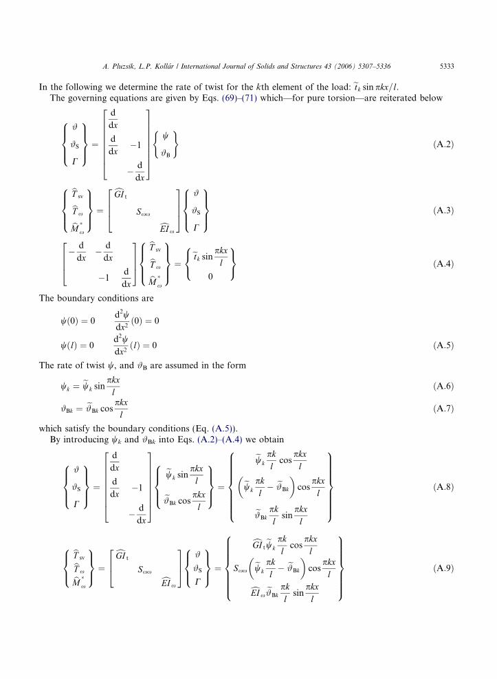
A. Pluzsik, L.P. Kollar / International Journal of Solids and Structures 43 (2006) 5307–5336 5333
In the following we determine the rate of twist for the kth element of the load: etk sin pkx=l.The governing equations are given by Eqs. (69)–(71) which—for pure torsion—are reiterated below
#
#S
C
8>><>>:9>>=>>; ¼
d
dx
d
dx�1
� d
dx
266666664
377777775w
#B
( )ðA:2Þ
bT svbT xbM �x
8>><>>:9>>=>>; ¼
cGI t
Sxx cEI x
26643775
#
#S
C
8>><>>:9>>=>>; ðA:3Þ
� d
dx� d
dx
�1d
dx
26643775
bT svbT xbM �x
8>><>>:9>>=>>; ¼
etk sinpkx
l
0
8<:9=; ðA:4Þ
The boundary conditions are
wð0Þ ¼ 0d2wdx2ð0Þ ¼ 0
wðlÞ ¼ 0d2wdx2ðlÞ ¼ 0 ðA:5Þ
The rate of twist w, and #B are assumed in the form
wk ¼ ewk sinpkx
lðA:6Þ
#Bk ¼ e#Bk cospkx
lðA:7Þ
which satisfy the boundary conditions (Eq. (A.5)).By introducing wk and #Bk into Eqs. (A.2)–(A.4) we obtain
#
#S
C
8>><>>:9>>=>>; ¼
d
dx
d
dx�1
� d
dx
266666664
377777775ewk sin
pkxl
e#Bk cospkx
l
8>><>>:9>>=>>; ¼
ewkpkl
cospkx
l
ewk
pkl� e#Bk
� �cos
pkxl
e#Bkpkl
sinpkx
l
8>>>>>>><>>>>>>>:
9>>>>>>>=>>>>>>>;ðA:8Þ
bT svbT xbM �x
8><>:9>=>; ¼
cGI t
Sxx cEI x
264375 #
#S
C
8><>:9>=>; ¼
cGI tewk
pkl
cospkx
l
Sxxewk
pkl� e#Bk
� �cos
pkxlcEI x
e#Bkpkl
sinpkx
l
8>>>>>><>>>>>>:
9>>>>>>=>>>>>>;ðA:9Þ

5334 A. Pluzsik, L.P. Kollar / International Journal of Solids and Structures 43 (2006) 5307–5336
� d
dx� d
dx
�1d
dx
26643775
bT svbT xbM �x
8><>:9>=>;¼
cGI tewk
p2k2
l2sin
pkxlþSxx
ewkp2k2
l2� e#Bk
pkl
� �sin
pkxl
�Sxxewk
pkl� e#Bk
� �cos
pkxlþcEI x
e#Bkp2k2
l2cos
pkxl
8>>><>>>:9>>>=>>>;¼
etk sinpkx
l0
8<:9=;ðA:10Þ
From these equations, after algebraic manipulation, we obtain
w ¼Xewk sin
pkxl
ðA:11Þ
ewk ¼l2
p2k2 cGI t þ Sxx 1� Sxx
Sxx þcEI xp2k2
l2
0BB@1CCA
0BB@1CCAetk ðA:12Þ
The rate of twist # is the derivative of w, which is
# ¼X e#k cos
pkxl
ðA:13Þ
e#k ¼l
pk cGI t þ Sxx 1� Sxx
Sxx þcEI xp2k2
l2
0BB@1CCA
0BB@1CCAetk ðA:14Þ
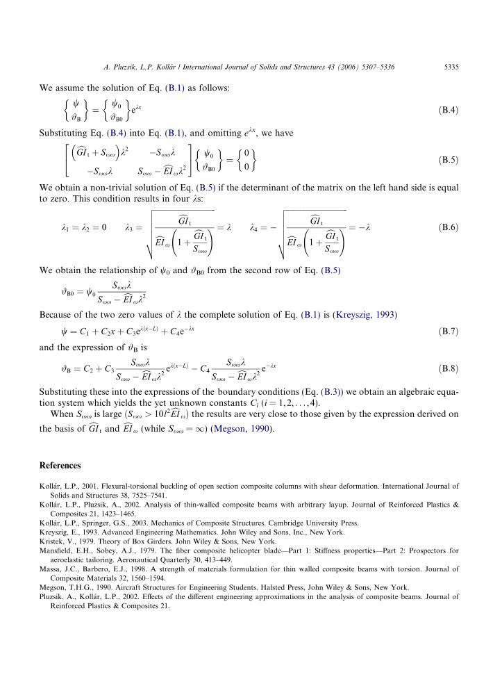
Appendix B. Cantilever beam subjected to a concentrated torque at the end
We consider a cantilever beam subjected to a torque bT at the end (Fig. 19).The governing equations are given by Eqs. (69)–(71), with t = 0.Substituting Eq. (70) into Eq. (71) and then into Eq. (69) we obtain
cGI t þ Sxx
� d2
dx2�Sxx
d
dx
�Sxxd
dxSxx �cEI x
d2
dx2
2666437775 w
#B
( )¼
0
0
( )ðB:1Þ
The boundary conditions are
wð0Þ ¼ 0 #Bð0Þ ¼ 0 ðB:2ÞbM �xðlÞ ¼ 0 bT ðlÞ ¼ bT
Using Eqs. (70), (71) and (3) we obtain
wð0Þ ¼ 0 #Bð0Þ ¼ 0
d#B
dxðlÞ ¼ 0 cGI t
dwdxðlÞ þ Sxx
dwdxðlÞ � #BðlÞ
� �¼ bT ðB:3Þ
A. Pluzsik, L.P. Kollar / International Journal of Solids and Structures 43 (2006) 5307–5336 5335
We assume the solution of Eq. (B.1) as follows:
w
#B
�¼
w0
#B0
�ekx ðB:4Þ
Substituting Eq. (B.4) into Eq. (B.1), and omitting ekx, we have
cGI t þ Sxx� k2 �Sxxk
�Sxxk Sxx �cEI xk2
24 35 w0
#B0
�¼
0
0
�ðB:5Þ
We obtain a non-trivial solution of Eq. (B.5) if the determinant of the matrix on the left hand side is equalto zero. This condition results in four ks:
k1 ¼ k2 ¼ 0 k3 ¼
ffiffiffiffiffiffiffiffiffiffiffiffiffiffiffiffiffiffiffiffiffiffiffiffiffiffiffiffiffiffiffifficGI t
cEI x 1þcGI t
Sxx
!vuuuuut ¼ k k4 ¼ �
ffiffiffiffiffiffiffiffiffiffiffiffiffiffiffiffiffiffiffiffiffiffiffiffiffiffiffiffiffiffiffifficGI t
cEI x 1þcGI t
Sxx
!vuuuuut ¼ �k ðB:6Þ
We obtain the relationship of w0 and #B0 from the second row of Eq. (B.5)
#B0 ¼ w0
Sxxk
Sxx �cEI xk2
Because of the two zero values of k the complete solution of Eq. (B.1) is (Kreyszig, 1993)
w ¼ C1 þ C2xþ C3ekðx�LÞ þ C4e�kx ðB:7Þ
and the expression of #B is#B ¼ C2 þ C3
Sxxk
Sxx �cEI xk2ekðx�LÞ � C4
Sxxk
Sxx �cEI xk2e�kx ðB:8Þ
Substituting these into the expressions of the boundary conditions (Eq. (B.3)) we obtain an algebraic equa-tion system which yields the yet unknown constants Ci (i = 1,2, . . . , 4).
When Sxx is large ðSxx > 10l2cEI xÞ the results are very close to those given by the expression derived on
the basis of cGI t and cEI x (while Sxx =1) (Megson, 1990).
References
Kollar, L.P., 2001. Flexural-torsional buckling of open section composite columns with shear deformation. International Journal ofSolids and Structures 38, 7525–7541.
Kollar, L.P., Pluzsik, A., 2002. Analysis of thin-walled composite beams with arbitrary layup. Journal of Reinforced Plastics &Composites 21, 1423–1465.
Kollar, L.P., Springer, G.S., 2003. Mechanics of Composite Structures. Cambridge University Press.Kreyszig, E., 1993. Advanced Engineering Mathematics. John Wiley and Sons, Inc., New York.Kristek, V., 1979. Theory of Box Girders. John Wiley & Sons, New York.Mansfield, E.H., Sobey, A.J., 1979. The fiber composite helicopter blade—Part 1: Stiffness properties—Part 2: Prospectors for
aeroelastic tailoring. Aeronautical Quarterly 30, 413–449.Massa, J.C., Barbero, E.J., 1998. A strength of materials formulation for thin walled composite beams with torsion. Journal of
Composite Materials 32, 1560–1594.Megson, T.H.G., 1990. Aircraft Structures for Engineering Students. Halsted Press, John Wiley & Sons, New York.Pluzsik, A., Kollar, L.P., 2002. Effects of the different engineering approximations in the analysis of composite beams. Journal of
Reinforced Plastics & Composites 21.
5336 A. Pluzsik, L.P. Kollar / International Journal of Solids and Structures 43 (2006) 5307–5336
Rehfield, L.W., Atligan, A.R., Hodges, D.H., 1988. Nonclassical behavior of thin-walled composite beams with closed cross section.In: American Helicopter Society National Technical Specialists� Meeting on Advanced Rotorcraft Structures, Williamsburg.
Roberts, T.M., Al-Ubaidi, H., 2001. Influence of shear deformation on restrained torsional warping of pultruded FRP bars of opencross-section. Thin-Walled Structures 39, 395–414.
Sapkas, A., Kollar, L.P., 2002. Lateral torsional buckling of composite beams with shear deformation. International Journal of Solidsand Structures 39, 2939–2963.
Urban, I.V., 1955. Teoria Rascota Sterznevih Tonkostennih Konstrukcij. Gosudarstvennoe Transportnoe ZeleznodoroznoeIzdatelstvo, Moscow.
Vlasov, V.Z., 1961. Thin-walled elastic beams. Office of Technical Services, US Department of Commerce, Washington 25, DC, TT-61-11400.
Wu, X., Sun, C.T., 1992. Simplified theory for composite thin-walled beams. AIAA Journal 30, 2945–2951.