i

Towards Efficient Scheduling of Federated Mobile Devices underComputational and Statistical Heterogeneity

Cong Wang, Member, IEEE, Yuanyuan Yang, Fellow, IEEE and Pengzhan Zhou

Abstract—Originated from distributed learning, federated learning enables privacy-preserved collaboration on a new abstracted level bysharing the model parameters only. While the current research mainly focuses on optimizing learning algorithms and minimizingcommunication overhead left by distributed learning, there is still a considerable gap when it comes to the real implementation on mobiledevices. In this paper, we start with an empirical experiment to demonstrate computation heterogeneity is a more pronounced bottleneckthan communication on the current generation of battery-powered mobile devices, and the existing methods are haunted by mobilestragglers. Further, non-identically distributed data across the mobile users makes the selection of participants critical to the accuracy andconvergence. To tackle the computational and statistical heterogeneity, we utilize data as a tuning knob and propose two efficientpolynomial-time algorithms to schedule different workloads on various mobile devices, when data is identically or non-identicallydistributed. For identically distributed data, we combine partitioning and linear bottleneck assignment to achieve near-optimal training timewithout accuracy loss. For non-identically distributed data, we convert it into an average cost minimization problem and propose a greedyalgorithm to find a reasonable balance between computation time and accuracy. We also establish an offline profiler to quantify theruntime behavior of different devices, which serves as the input to the scheduling algorithms. We conduct extensive experiments on amobile testbed with two datasets and up to 20 devices. Compared with the common benchmarks, the proposed algorithms achieve2-100× speedup epoch-wise, 2-7% accuracy gain and boost the convergence rate by more than 100% on CIFAR10.

Index Terms—Federated learning; on-device deep learning; scheduling optimization; non-IID data.

F

1 INTRODUCTION

The tremendous success of machine learning stimulates anew wave of smart applications. Despite the great conve-nience, these applications consume massive personal data, atthe expense of our privacy. The growing concerns of privacybecome one of the major impetus to shift computation fromthe centralized cloud to users’ end devices such as mobile,edge and IoTs. The current solution supports running on-device inference from a pre-trained model in near real-time [23], [24], whereas their capability to adapt to the newdata and learn from each other is still limited.

Federated Learning (FL) emerges as a practical and cost-effective solution to mitigate the risk of privacy leakage [2],[4]–[6], [8]–[12], which enables collaboration on an abstractedlevel rather than the raw data itself. Originated from dis-tributed learning [1], it learns a centralized model where thetraining data is held privately at the end users. Local modelsare computed in parallel and the updates are aggregatedtowards a centralized parameter server. The server takes themean of the parameters from the users, pushes the averagedmodel back as the initial point for the next iteration. Previousresearch mainly focuses on the prominent problems leftfrom distributed learning such as improving communicationefficiency [8]–[13], security robustness [19], [20], or thelearning algorithms [12] to address new challenges in FL.

Most of these works only contain proof-of-concept im-plementations on cloud/edge servers with stable, externalpower and proprietary GPUs. Though pioneering effortsto improve FL at the algorithm level, they still leave a

• Cong Wang is with the Department of Computer Science, Old DominionUniversity, Norfolk, VA, USA, E-mail: c1wang@odu.edu

• Yuanyuan Yang and Pengzhan Zhou are with the Department of Electricaland Computer Engineering, Stony Brook University, NY, USA, E-mail:{yuanyuan.yang, pengzhan.zhou}@stonybrook.edu

• Correspondence to c1wang@odu.edu.

gap to the system-level implementations at the mobile datasource, where FL was originally targeting at. Meanwhile, thedramatic increase of mobile processing power has enablednot only on-device inference, but also moderate training(backpropagation) [6], [7], [27], thus providing a basis tolaunch FL on battery-powered mobile devices.

Unfortunately, the vast heterogeneity of mobile process-ing power has yet to be addressed. Even worse, the highvariance among user data adds another layer of statisticalheterogeneity [12] and makes the selection of participantsa nontrivial problem. An inappropriate selection wouldadversely cause gradient divergence and diminish everyeffort to reduce computation time. From an empirical study,we first validate that the bottleneck has actually shiftedfrom communication back to computation on consumermobile devices. The runtime behavior depends on a complexcombination of vendor-specific software implementationsand the underlying hardware architecture, i.e., the Systemon a Chip (SoC), power management policies and theinput computation intensity of the neural networks. Thesechallenges are magnified in practices when users behavedifferently. For example, in activity recognition, some usersmay perform only a few actions (e.g., sitting for a long time),thus leading to highly skewed local distributions, whichbreaks the independent and identically distributed (IID)assumptions held as a basis for distributed learning. Whenaveraged into the global model, these skewed gradientsmay have a damaging impact on the collaborative model.Thus, efficient scheduling of FL tasks entails an optimalselection of participants relying on both computation anddata distribution.

To tackle these challenges, we propose an optimizationframework to schedule training using the workloads (amountof training data) as a tuning knob and achieve near-optimalstaleness in synchronous gradient aggregation. We build aperformance profiler to characterize the relations between

arX

iv:2

005.

1232

6v2

[cs

.LG

] 1

5 Se

p 20

20

ii

training time and data size/model parameters using amultiple linear regressor. Taking the profiles as inputs, westart with the basic case when data is IID (class-balanced),and formulate the problem into a min-max optimizationproblem to find optimal partitioning of data that achievesthe minimum makespan. We propose an efficient O(n2 log n)algorithm [37] with O(n) analytical solution when the costfunction is linear (n is the number of users). For non-IIDdata, we introduce a new accuracy cost and a quantitativederivation from the analysis of gradient diversity [34]. Thenwe re-formulate the problem into a min average cost problemand develop a greedy O(mn)-algorithm to assign workloadswith the minimum average cost in each step using a variationof bin packing [40] (m is the number of data shards). Theobservation suggests a nontrivial trade-off between stalenessand convergence. The proposed algorithm aims to leverageusers’ class distributions to adaptively include/exclude anoutlier in order to improve model generalization and conver-gence speed without sacrificing the epoch-wise training timetoo much. Finally, the proposed algorithms are evaluatedon MNIST and CIFAR10 datasets with a mobile testbed ofvarious smartphone models.

The main contributions are summarized below. First,we motivate the design by a series of empirical studiesof launching backpropagation on Android. This expandsthe current research of FL with new discoveries of thefundamental cause of mobile stragglers, as well as offeringan explanation to the subtlety in non-IID outliers throughthe lens of gradient diversity. Second, we formulate theproblem to find the optimal scheduling with both IID andnon-IID data, and propose polynomial-time algorithms withanalytical solutions when the cost profile is linear. Finally,we conduct extensive evaluations on MNIST and CIFAR10datasets under a mobile testbed with 6 types of device com-binations (up to 20 devices). Compared to the benchmarks,the results show 2-100× speedups for both IID/non-IID datawhile boosting the accuracy by 2-7% on MNIST/CIFAR10for non-IID data. The algorithms demonstrate advantagesof avoiding worst-case stragglers and better utilization ofthe parallelled resources. In contrast to the existing worksthat decouple learning from system-level implementations,to the best of our knowledge, this is the first work that notonly connects them, but also optimizes the overall systemperformance.

The rest of the paper is organized as follows. Section2 discusses the related works and background. Section 3and 4 motivate this work with a series of empirical studies.Sections 5 and 6 optimizes training time for IID and non-IIDdata. Section 7 describes the profiler. Section 8 evaluatesthe framework on the mobile testbed and dataset. Section 9discusses the limitation and Section 10 concludes this work.

2 BACKGROUND AND RELATED WORKS

2.1 Deep Learning on Mobile DevicesThe continuous advance in mobile processing power, batterylife and improvement of power management reaches itsculminating point with the debut of AI chips [21], [22]. Theirpower spans from executing simple algorithms like logisticalregression or supported vector machine, to the resource-intensive deep neural networks. The research communityquickly embraces the idea to migrate inference computations

off the cloud to the mobile device, and develops newapplications for better user interaction and experience [23],[24]. To fit the neural network within the memory capacity,some optimization is necessary such as pruning the near-zero parameters via compression [25] or directly learninga sparse network before deployment [26]. Recently, thereare new efforts to incorporate the entire training process onmobile devices for better privacy preservation and adaptationof the new patterns in data distribution [7], [27]. Theirimplementation attempts to close the loop of the learningprocess from data generation/pre-processing to decisionmaking all on user’s end devices, which has also laid thefoundation of this paper.

The implementation of federated learning on mobiledevices is subject to physical limitations from the memoryand computation. Unlike desktop or cloud servers that theGPUs have dedicated, high-bandwidth memory, the memoryon consumer mobile devices is extremely limited. The mobileSoC typically has unified memory, where the mobile GPUonly has some limited on-chip buffer. Further, on the OS-level,Android has limited memory usage for each application (e.g.,setting the LargeHeap would give the application 512 MB).Though using the native code can bypass the limit, it is stillsubject to the memory limits about 3-4GB on most mobiledevices, where a majority is shared by other system processes.This largely constrains us from running ultra-deep models.As shown later, the bottleneck still lies in the computationalside due to limited paralleled resources, since most mobiledevices have about 8 CPU cores and similar number of GPUshader cores. Thus, it is expected that the computation timewould increase parabolically with a more complex neuralnetwork model, especially on the lowgrade devices.

The collaboration of mobile devices brings more uncer-tainties to the system. Vendors typically integrate different IPblocks under the area and thermal constraints, thus resultinga highly fragmented mobile hardware market: 1) unlike theubiquitous of CUDA to accelerate cloud GPUs, programmingsupport is inadequate for mobile GPUs; 2) most mobile GPUshave similar computational capability compared to the multi-core CPUs [50]. Thus, for better programming support, weexecute learning by the multi-core CPUs in this paper.

Like any other applications in the userspace, the learningprocess is handled by the Linux kernel of Android, whichcontrols cpufreq by the CPU governor in response to theworkload. For example, the default interactive governorin Android 8.0 scales the clockspeed over the course of atimer regarding the workload. For better energy-efficiencyand performance, off-the-shelf smartphones are often em-bedded with asymmetric multiprocessing architectures, i.e.,ARM’s big.LITTLE [28]. For instance, Nexus 6P is poweredby octa-core CPUs with four big cores running at 2.0 GHzand four little ones at 1.53 GHz. The design intuition isto handle the bursty nature of user interactions with thedevice by placing low-intensity tasks on the small cores, andhigh-intensity tasks on the big cores. However, the behaviorof such subsystem facing intensive, sustained workloadsuch as backpropagation remains underexplored. Further,since vendors usually extend over the vanilla task schedulerthrough proprietary designs of task migration/packing, loadtracking and frequency scaling, the same learning taskwould incur heterogenous processing time depending onthe hardware and system-level implementation. Our goal is

iii

to mitigate such impact on FL while still using the defaultgovernor and scheduler for applications in the userspace.

2.2 Federated Learning

McMahan et al. introduce FedAvg that averages aggre-gated parameters from the local devices and minimizesa global loss [2]. Formally, for the local loss functionlk(·)(k ∈ {1, 2, · · · , N}) of N mobile devices, FL minimizesthe global loss L by averaging the local weights w,

minw

{L(w) =

N∑k=1

lk(w)}. (1)

In each round, mobile device k performs a number of E localupdates,

wki+1 = wk

i − ηi∇lk(wki ), (2)

with learning rate ηi and i = {0, 1, · · · , E}. The local updateswkE are aggregated towards the server for averaging, and

the server broadcasts the global model to the mobile devicesto initiate the next round. From the user’s persecutive, onemay advocate designs without much central coordination. Asmost of the FL approaches pursue the first-order synchronousapproach [2], [4]–[6], [8]–[10], the starting time of the nextround is determined by the straggler in the last round,who finishes the last among all the users. Hence, from theservice provider’s perspective, it is far from efficient due tothe straggler problem. It leads to slower convergence andgenerates a less performing model with low accuracy andultimately undermines the collaborative efforts from all theusers.

A solution is to switch to asynchronous update [14], [15].Asynchronous methods allow the faster users to resumecomputation without waiting for the stragglers. However,inconsistent gradients could easily lead to divergence andamortize the savings in computation time. Though it ispossible to estimate the gradient of the stragglers usingsecond-order Taylor expansion, the computation and mem-ory cost of the Hessian matrix become prohibitive forcomplex models [14]. In the worst case, gradients from thestragglers that are multiple epoches old could significantlydivert model convergence to a local minima. For example,the learning process typically decreases the learning rateto facilitate convergence on the course of training. Thestragglers’s stale gradients with a large learning rate wouldexacerbate such divergence [16]. The practical solution fromGoogle is to simply drop out the stragglers in large scaleimplementation [6]. Yet, for those small-scale federated tasks,e.g., learning from a small set of selected patients with raredisease, such hard drop-out could be detrimental to modelgeneralization and accuracy. Gradient coding [17] replicatescopies of data between users so when there is a slow-down,any linear combination from the neighbors can still recoverthe global gradient. It is suitable for GPU clusters, where allthe nodes are authenticated and data can be moved withoutprivacy concerns. Nevertheless, sharing raw data amongusers defeats the original privacy-preserving purpose of FL,thereby rendering such pre-sharing method unsuitable fordistributed mobile environments.

As a key difference from distributed learning, non-IIDness is discussed in [3]–[5]. It is shown in [3] thatfor strongly convex and smooth problems, FedAvg still

retains the same convergence rate on non-IID data. However,convergence may be brittle for the rest non-convex majoritieslike multi-layer neural networks. As a remedy, [4] pre-sharesa subset of non-sensitive global data to mobile devicesand [5] utilizes a generative model to restore the data back toIID, but at non-negligible computation, communication andcoordination efforts. Another thread of works address thecommon problem of communication efficiency in FL [8]–[13].The full model is compressed and cast into a low-dimensionalspace for bandwidth saving in [8]. Local updates thatdiverge from the global model are identified and excludedto avoid unnecessary communication [9]. Decentralizedapproaches and convergence are discussed in [10] whenusers only exchange gradients with their neighbors. Evolu-tionary algorithm is explored to minimize communicationcost and test error in a multi-objective optimization [11].The challenges from system, statistics and fault toleranceare jointly formulated into a unified multi-task learningframework [12]. A new architecture is proposed with tieredgradient aggregation for saving network bandwidth [13].Such aggregation re-weights the individual’s contribution tothe global model, that may unwittingly emphasize the shareof non-IID users. As recommended by [18], a practical wayto save the monetary cost of communication is to scheduleFL tasks at night when the devices are usually chargingand connected to WiFi. These efforts are orthogonal to ourresearch and can be efficiently integrated to complement ourdesign.

Our study has fundamental difference from a large bodyof works in scheduling paralleled machines [31]–[33]. First,rather than targeting at jobs submitted by cloud users, wedelve into a more microcosmic level and jointly considerpartitioning a learning task and makespan minimization,where the cost function is characterized from real experimen-tal traces. Second, FL calls for the scheduling algorithmto be aware of non-IIDness and model accuracy whenworkloads are partitioned. Hence, our work is among thefirst to address computational and statistical heterogeneityon mobile devices.

3 COMPUTATION VS. COMMUNICATION TIME

0 10 20 30 40 50 60

Data batch (batchsize=20)

100

101

102

Tim

e (

s)

Training time per batch (LeNet-MNIST)

Nexus 6

Nexus 6P

Samsung J8

Mate 10

Pixel 2

Huawei P30

0 10 20 30 40 50 60

Data batch (batchsize=20)

101

102

103

Tim

e (

s)

Training time per batch (VGG-MNIST)

Nexus 6

Nexus 6P

Samsung J8

Mate 10

Pixel 2

Huawei P30

(a) (b)Fig. 1: Benchmark training time on different mobile devices(MNIST dataset) (a) LeNet (b) VGG6 (best view in color)

In this section, we are motivated to answer the basicquestion: how large is the gap of the computational time amongmobile devices and how does it compare to communication? Wedemonstrate this through an empirical study to launcha training application using neural network models ofLeNet [38] and VGG6 [39] on the mobile testbed (shownin Table 1 in Sec. 8).

iv

To benchmark the computation time, we trace the trainingtime per data batch (20 samples) on different devicesshown in Fig. 1 and the average of CPU clock speedevery 5s vs. the temperature in Fig. 3. Though the CPUscan switch frequencies much faster, this experiment showshow the frequency and temperature interact over time toreach stability under the power management policy (in/system/etc/thermal-engine.conf).

LeNet - 3K samples (5% of MNIST)

Nex

us6

Nex

us6P J8

Mat

e10

Pixel2

P300

20

40

60

80

Tim

e (

s)

Computation Time

WiFi Comm. Time

LTE Comm. Time

6.5%

5.4%

4.5%

10.9%

8%

3%

VGG6 - 3K samples (5% of MNIST)

Nex

us6

Nex

us6P J8

Mat

e10

Pixel2

P3010

2

103

Tim

e (

s)

Computation Time

WiFi Comm. Time

LTE Comm. Time2.6%

12.0%13.9% 14.6%

25.5%

10.4%

(a) (b)Fig. 2: Computation vs. communication time of training onMNIST samples per epoch (s) (a) LeNet (b) VGG6

To measure the communication time, we establish anAWS server for communicating the model between the cloud(Washington D.C.) and local devices (Norfolk, VA). Theserver pushes (pulls) the model to (from) the devices ineach epoch and iterates through 5% of the dataset with 3Ksamples. We measure the transmission time of the LeNet(2.5MB) and VGG6 (65.4MB) model over the 1 Gbps wirelesslink and T-mobile 4G LTE (-94 dBm), to emulate differentnetworking environments. The WiFi uplink/downlink speedachieves around 80-90 Mbps on our campus network andLTE reaches about 60 Mbps and 11 Mbps for the uplinkand downlink respectively. The makespan for each deviceis shown in Fig. 2 with the percentage of communicationoverhead on top. Based on all the experiments above, wesummarize the observations below.

3.1 Key ObservationsObservation 1. Computation time is mainly governed bythe processing power/performance of the CPUs/SoC (withsome variations from the OEM implementations), as well asthe computation intensity of the neural network model.Observation 2. The continuous neural computation leadsto thermal throttling, where the governor quickly reactsto reduce the cpufreq, or even shuts down some cores,thereby causing a performance hit with large variance in thesubsequent batch iterations (especially running heavy-weightnetworks like VGG6 on Nexus6/6P). Such phenomenon addsto the diversity of computation time.Observation 3. In contrast to the hypothesis in [2] thatcommunication overhead dominates in FL, our experimentsindicate that communication only takes a small portion ofthe training time (below 10% on average as seen in Fig.2). This confirms that with today’s networking speed andthe upcoming 5G, the bottleneck of FL on battery-poweredmobile devices is expected to remain on the computationalside. Part of the reason is because the consumer mobiledevices cannot host heavy-weight neural architectures (suchas increasing VGG6 to 16 layers), which easily overwhelm thememory limit of 512 MB per application set by Android [29].Even if more memory is permitted to execute large models,

the bottleneck would still remain on the computational sidebecause of the parabolical increase of computation time,compared to the relatively linear increase in communicationtime.Observation 4. To process the same amount of data, themobile devices exhibit substantial heterogeneity in theircompletion time. For example, the straggler takes morethan 3× compared to the mean completion time from otherdevices, and this deviation is expected to get larger withhigher workloads such as more complex models or dataiterations.

3.2 CPU Frequency vs. Temperature

We observe two major factors: hardware architecture andthermal throttling, that impact the computation speed forsuch sustained workloads of running backpropagation. Ofcourse, speed is dominated by the hardware architecturesuch as the CPUs/SoC, and should be in general consistentand predictable with the hardware configurations. However,unlike desktops, thermally constrained mobile devices resulthigher diversity in runtime as per to the different workloadsand computation intensity.

0 10 20 30 40 50 60

Data batch (20 samples/batch)

1

1.5

2

2.5

3F

req

. (G

Hz)

Nexus 6: CPU Frequency

0 10 20 30 40 50 60

Data batch (20 samples/batch)

60

70

80

90

Te

mp

. (C

els

ius)

Nexus 6: Temperature

0 10 20 30 40 50 60

Data batch (20 samples/batch)

0

0.5

1

1.5

2

Fre

q.

(GH

z)

Nexus 6P: CPU Frequency

Small Cluster

Big Cluster

0 10 20 30 40 50 60

Data batch (20 samples/batch)

40

50

60

70

Te

mp

. (C

els

ius)

Nexus 6P: Temperature

Small Cluster

Big Cluster

(a) (b)

0 10 20 30 40 50 60

Data batch (20 samples/batch)

1.6

1.8

2

2.2

2.4

Fre

q.

(GH

z)

Mate10: CPU Frequency

Small Cluster

Big Cluster

0 10 20 30 40 50 60

Data batch (20 samples/batch)

40

50

60

70

80

Te

mp

. (C

els

ius)

Mate10: Temperature

Small Cluster

Big Cluster

0 10 20 30 40 50 60

Data batch (20 samples/batch)

1.65

1.7

1.75

1.8

1.85

Fre

q.

(GH

z)

Samsung J8: CPU Frequency

0 10 20 30 40 50 60

Data batch (20 samples/batch)

45

50

55

60

Te

mp

. (C

els

ius)

Samsung J8: Temperature

(c) (d)

Fig. 3: CPU clock speed vs. temperature. (a) Nexus6 (b)Nexus6P (c) Mate10 (d) SamsungJ8.

We show the trace of CPU frequency and temperatureof four devices in Fig. 3. Before analyzing the results, webriefly describe their CPU microarchitectures: 1) Nexus 6 hasa single quad-core CPU cluster running at 2.7GHz; 2) Nexus6P has octa-core CPU clusters. The four big cores are runningat 2.0 GHz and the four little cores are running at 1.55 GHz;3) Mate10 also has octa-core CPU clusters. The four big coresare running at 2.4 GHz and the four little cores are runningat 1.8 GHz; 4) SamsungJ8 features octa-core all running at1.8GHz in a single cluster. All of them are the maximumfrequencies of the CPU. For clarity, we average the frequencyand temperature for all the homogeneous cores in Fig. 3.

We can see that different devices exhibit distinct behaviorsof how the governor reacts to temperature surge. Nexus6 allows the temperature to stay above 60◦C and even

v

surpass the 70◦C level, in exchange for running the CPUonly 20-30% below the max. frequency. In contrast, Nexus6Pis more conservative due to the controversial Snapdragon810 SoC [35]. It actively reduces the frequency of the big coresto below 50%, and even switches off all the cores in the bigcluster, in order to maintain the temperature around 50◦C.The big cores go offline and migrate the tasks to the littlecores after a moderate temperature surge, that occurs fairlyoften during the testing. The big cores never stay aroundtheir maximum frequency at 2.0 GHz, thus making Nexus 6Pmuch slower than Nexus 6 even with more CPU cores. Therecent generations of Mate10 and Samsung J8 exhibits morestability. The governors manage to maintain the temperaturearound 50◦C with only 20-30% discounted clockspeed.

The throttling process is controlled by the vendor-specificdriver for frequency scaling. Obviously, Nexus 6 has a morerelaxed throttling temperature, which allows the CPUs tostay at high frequency and persistently online than Nexus 6P.Such possible overclocking has made it outclass the newerversions of Mate10 on some low intensity tasks (about 3×speedup calculated in from Fig. 1(a)), though Nexus 6 backin 2014 were not designed for intensive workload like neuralcomputations. These experimental studies suggest that weshould factor in both the device-specific characteristics andthe workload intensity in estimating the computation time.

Since FL takes more than 10 epoches to converge, asshown in Fig. 2, only processing 5% MNIST for 10 epochesleads to 0.7 to 2.6 hours time difference to wait for thestragglers. If each model update entails more local itera-tions, this delay is expected to increase exponentially (withmore thermal throttling on the stragglers). An optimizedscheduling mechanism should be built to account for thesefactors. In cloud environments, stragglers may be caused byresource contention, unbalanced workload or displacementof workers on different parameter servers [32], which aretypically handled by load balancing. In mobile environment,they are caused by the fundamental disparity among users’devices: can we do the opposite and leverage load unbalancingto offset the computation time of those stragglers? If so,what about the side effects and how to mitigate? Sinceeach epoch requires a full pass of the local data, amonga variety of tunable knobs, workload is directly proportionalto the amount of training data. Nevertheless, distributedlearning often assumes a balanced data partition among theworkers [2]. Would data imbalance (either in the case of IIDor non-IID data distribution) lead to significant accuracyloss? We further study additional impact from the datadistributions before formulating our problem.

4 IMPACT OF DATA DISTRIBUTIONS

4.1 Impact of Data Imbalance to IID DataWe partition the datasets of MNIST and CIFAR10 among20 users. E.g., for MNIST, the training set of 60K imagesresults an average of 3K images per user. Then we utilize aGaussian distribution to sample around the mean and adjustthe standard deviation to induce data imbalance amongusers. The ratio between different classes is uniform so noclass dominates the local set. We utilize an index of imbalanceratio between the standard deviation and the mean as thex-axis (larger ratio means more extreme), and benchmarkthe accuracy against the centralized and distributed learning

0 0.2 0.4 0.6 0.8

Imbalance ratio

97

97.5

98

98.5

99

99.5

Te

st

Accu

racy (

%)

Impact of data imbalance on accuracy (MNIST)

Centralized (Baseline)

Distributed (Balanced)

Distributed (imbalanced)

Trend Line

(a)

0 0.2 0.4 0.6 0.8 1

Imbalance ratio

56

58

60

62

64

66

68

70

Te

st

Accu

racy (

%)

Impact of data imbalance on accuracy (CIFAR)

Centralized (Baseline)

Distributed (Balanced)

Distributed (Unbalanced)

Trend Line

(b)Fig. 4: Impact of data imbalance (still IID) on FL accuracy (a)MNIST (b) CIFAR10

with balanced data in Fig.4. The results indicate that as longas the data remains IID, imbalance does not lead to accuracyloss. It is reasonable since the local gradients still resembleeach other when data is IID. The accuracy even trends up alittle for CIFAR10. This provides the basis for optimizationdiscussed in the next section.

4.2 Impact of non-IID DataNon-IIDness is shown to have negative impact on collabora-tive convergence [2], [4] and data imbalance could exacerbatethis issue. Instead of investigating data imbalance and non-IIDness together, we investigate how non-IID data aloneis enough to impact accuracy and convergence. We seekanswers to the fundamental question: How can we identifyand deal with the users having non-IID distributions? Weightdivergence, ‖wi −

∑Ni=1 wi/N‖22 is used in [4] to compare

the norm difference between the local weights wi and theglobal average. Local loss is an equivalent indicator withless complexity, since it does not require pairwise weightcomputations. Fig. 5(a) compares the local loss of the non-IIDoutlier with the average loss from the rest users and the idealcase when the data is IID. The outlier user with only oneclass can be easily identified from the rest IID ones, whichhas over an order of magnitude loss value and is unable toconverge compared to the rest.

While identifying outliers is simple, the existing stud-ies [4], [5], [9] have yet to reach a consensus on howto deal with them. With the outlier user only having asubset of classes, our intuition is that accuracy is directlyassociated with the distribution of classes among the users [9].To see how the number of classes impacts accuracy, weconduct the second experiment by iterating the number ofclasses per user from 2-8 (out of 10 classes) plus a standarddeviation of samples among the existing classes as the x-axis. It is observed in Fig. 5(b) that higher disparity of classdistributions among the users indeed leads to more accuracydegradation with a substantial loss of 10-15% on CIFAR10.

Since the presence of non-IID outliers is inevitable inpractices, we are facing two options: 1) simply exclude themfrom the population based on loss divergence [9]; 2) keepthem in training. We take a closer look of these options andargue that the decision should be actually conditioning onthe class distributions, rather than only based on the localloss or weight divergence. We demonstrate through a simplecase to distribute CIFAR10 dataset among 4 users in differentways, and introduce a fifth user to act as the non-IID outlier.

• Ideal IID(10): the ideal baseline when all 4 users haveidentical distribution and all 10 classes are evenlydistributed among them.

vi

0 10 20 30 40 5010

0

101

102

Te

st

Lo

ss (

loca

l)

Loss comparison of non-IID outlier

Outlier-one user (Non-IID)

Mean-rest users (IID)

Ideal (IID)

(a)

2 3 4 5 6 7 8

Avg # of classes per user (total 10 classes)

35

40

45

50

55

Te

st

Accu

racy (

%)

Impact of non-IID data (CIFAR10-LeNet)

Test accuracy

Trendline

(b)

Fig. 5: Impact of non-IID data on local convergence andmodel accuracy (CIFAR10) (a) comparison of local loss (b)relation between the degree of non-IID class distribution andaccuracy.

• Include Non-IID(10): the population has 10 classes. Afifth user with only one class is included, but herclass has already presented in the population. Thepopulation becomes non-IID because of the fifth user.

• Include Non-IID(9): the population has 9 classes. Afifth user with that missing class (one-class outlier) isincluded. The population is also non-IID.

• Exclude IID(9): the population has 9 classes. Excludethe fifth user despite she possesses class samples fromthe missing class so the population remains IID [9].

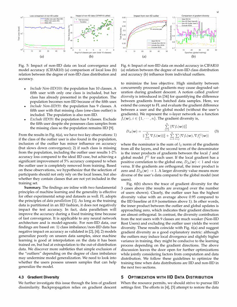
From the results in Fig. 6(a), we have two key observations: 1)if the class of the outlier user is also found in the population,inclusion of the outlier has minor influence on accuracy(but slows down convergence); 2) if such class is missingfrom the population, including the outlier user results 1-2%accuracy loss compared to the ideal IID case, but achieving asignificant improvement of 5% accuracy compared to whenthe outlier user is completely removed from training. Basedon these observations, we hypothesize that the selection ofparticipants should not only rely on the local losses, but alsowhether they contain classes that are not yet included in thetraining set.

Summary. The findings are inline with two fundamentalprinciples of machine learning and the generality is effectivefor other experimental setup and datasets as well. FL adoptsthe principles of data parallelism [1]. As long as the trainingdata is partitioned in an IID fashion, it does not negativelyimpact the test accuracy. In fact, data parallelism willimprove the accuracy during a fixed training time becauseof fast convergence. It is applicable to any neural networkarchitecture and is model-agnostic. For non-IID data, ourfindings are based on: 1) class imbalance/non-IID data hasnegative impact on accuracy as validated in [2], [4]; 2) modelsgeneralize poorly on unseen data samples, since machinelearning is good at interpolation on the data it has beentrained on, but bad at extrapolation to the out-of-distributiondata. We discover more subtleties that simple exclusion ofthe “outliers” depending on the degree of class imbalancemay undermine model generalization. We need to look intowhether the users possess unseen samples that can helpgeneralize the model.

4.3 Gradient DiversityWe further investigate this issue through the lens of gradientdissimilarity. Backpropagation relies on gradient descent

0 10 20 30 40 50

0.3

0.35

0.4

0.45

0.5

0.55

0.6

0.65

Te

st

Accu

racy

Impact from non-IID outlier

Ideal IID(10)

Include Non-IID(10)

Include Non-IID(9)

Exclude IID(9)

5% accuracy gap

(a)

0 10 20 30 40 50

Epoches (global training)

0.7

0.8

0.9

1

1.1

1.2

Gra

die

nt

div

ers

ity

Comparison of gradient diversity

Ideal IID(10)

Non-IID Rest Users(9)

Non-IID Outlier User(1)

Exclude IID(9)

(b)

Fig. 6: Impact of non-IID data on model accuracy in CIFAR10(a) relation between the degree of non-IID class distributionand accuracy (b) influence from individual outliers.

to minimize the loss objective. High similarity betweenconcurrently processed gradients may cause degraded sat-uration during gradient descent. A notion called gradientdiversity is introduced in [34] for quantifying the differencebetween gradients from batched data samples. Here, weextend the concept to FL and evaluate the gradient differencebetween a user and the global model (without the user’sgradients). We represent the n-layer network as a functionfi(w), i ∈ {1, · · · , n}. The gradient diversity is,

D∆(w) =

n∑i=1

‖∇fi(w)‖22

‖n∑i=1

∇fi(w)‖22 +n∑i=1

∑i=j

〈∇fi(w),∇fGj (w)〉(3)

where the nominator is the sum of l2 norm of the gradientsfrom all the layers, and the second term of the denominatoris the inner products of gradients between the local f andglobal model fG for each user. If the local gradient has apositive correlation to the global one, D∆(w) < 1 and viceversa. If the gradients are orthogonal, the inner product iszero and D∆(w)→ 1. A larger diversity value means morediverse of the user’s data compared to the global model (restusers).

Fig. 6(b) shows the trace of gradient diversity for the3 cases above (the results are averaged over the numberof users shown). Clearly, the outlier user has the highestdiversity value with an average above 0.95 compared tothe IID baseline at 0.9 (sometimes above 1). In other words,the inner product between the outlier and global updates isapproaching zero, which indicates their gradient directionsare almost orthogonal. In contrast, the diversity contributionfrom the rest users with 9 classes are much weaker (Non-IIDRest Users) and excluding the outlier user yields the worstdiversity. These results coincide with Fig. 6(a) and suggestgradient diversity as a good explanatory metric: althoughthe outliers may induce local divergence and slightly highervariance in training, they might be conducive to the learningprocess depending on the gradient directions. The abovediscussion leaves the door open for further optimizationswhile jointly considering factors from computation and datadistribution. We follow these guidelines to optimize thetraining time when data distributions are IID and non-IID inthe next two sections.

5 OPTIMIZATION WITH IID DATA DISTRIBUTION

When the resource permits, we should strive to pursue IIDsettings first. The efforts in [4], [5] attempt to restore the data

vii

back into IID. On the other hand, a partial reason of non-IIDness is due to the imperfect data collection process. Forexample, the collection period is inadequate or a necessarydata cleaning/augmentation is missing. With the abundanceof mobile data, the scheduler can ask the users to carefullyselect the data from a sufficiently longer period of time.Meanwhile, the application could also incentivize users toperform those activities that are needed in order to remainIID defined by the task objectives. To this end, we start withthe case that the local dataset contains data from all theclasses (i.e., IID) and optimize the training time per epoch inthis section.

5.1 System ModelThe success of machine learning algorithms relies on a largeand broad dataset. The goal is to minimize the expectedgeneralization error between training and testing by fittingthe distributions of D data. A theoretical bound between theamount of data needed for achieving certain error rates isavailable in [30]. The FL training task requires a total amountof data D, where D can be either obtained empiricallyor estimated using [30]. We use shards to represent theminimum granularity of samples (e.g. 100 samples/shard).The parameter server has sufficient bandwidth and simul-taneous transmissions do not cause network congestion orperformance saturation [6]. Our framework mainly tacklesheterogeneity from computation and data distribution, andis amenable to decentralized topologies without a parameterserver [10]. The users will agree on a protocol to executetraining from the demanded amount of data requested bythe scheduler. The training data can be a subset of the localdata collected during a long time period. For comparisonand reproducibility, we follow the same approach as [2],[4] to partition public datasets on different devices. Wedelegate the role of management to the server to gatherusers’ meta data such as smartphone model and informationabout non-IID class distribution. For simplicity, we assumethe server is honest and does not attempt to infer userprivacy from the collaborative model or class informationas we can always resort to security protocols to protect theintermediate gradients, model and differentially-private classinformation [19]. We formalize the optimization problem forIID data distributions next.

5.2 Problem Formulation (IID)FL follows the stochastic gradient descent to randomly selecta number of users for training in each epoch [2]. Our objectiveis to optimize the execution time of the selected n = |N |users. As shown in Section 4.1, we can leverage unbalancedlocal data with minimum accuracy loss as long as the datais IID among the users. This gives enough latitude for taskassignments. For all the permutations φ that partition thetotal data D, the computation time T ci (Di) for user i is afunction of her data size Di. Depending on the networkingenvironments, the uplink and downlink network latency foruser i is a linear function of model size M , Tui (M)+T di (M).Our goal is to find an optimal assignment of training data sothat the maximum processing time is minimized per epoch.The problem is formalized below.

P1 : minDi∈φ

maxi∈N

(T ci (Di) + Tui (M) + T di (M)

)(4)

s.t. ∑i∈N Di = D, (5)

φ = {D1, D2, · · · , Dn}. (6)∑i∈N xi = n (7)

The objective in Eq. (4) is to minimize the makespan givenall possible data partitions and the assignment of Di datato user i. Eq. (5) states that the sum of local data shouldbe equal to D. Eq. (6) denotes the permutations of all datapartition. For completeness, Eq. (7) requires all the users toparticipate in training. The decision variable xi = 1 if a userparticipates; otherwise, it is zero.

P1 can be viewed as a combination of a partitioningproblem and a variant of the linear bottleneck assignment problem(LBAP) [36]. The classic assignment problem finds an optimalassignment of workers to tasks with minimum sum of cost.LBAP is its min-max version. It assigns tasks to parallelworkers and ensures the latest worker uses minimum time.We adopt the same analogy here to ensure each trainingepoch is finished in minimum time. The problem is differentfrom both the classic assignment problem and LBAP. Thenumber of potential tasks is not equal to the number ofworkers (mobile devices), but rather, a much wider potentialrange to choose from due to the combinatorial partitions ofthe dataset. The final choice would be determined by the setof constraints that optimizes Eq. (4). A naive solution is tolist all the partitions of D in brute force, construct cost valuesper user for all the potential permutations, solve an LBAPand find the assignment with the minimum makespan. Fora total number of s shards, the possible permutations are inthe order of sn, which makes it intractable even for small n.

5.3 Joint Partitioning and Assignment

Though the naive method turns out to be futile in polynomialtime, the following property of mobile devices helps simplifythe problem.Property 1. For data Di, T ci (Di) + Tui (M) + T di (M) is anon-decreasing function.

Then it is not necessary to test a large number of potentialpartitions, if a partition of smaller size has already satisfiedEq. (5) with less computation time. For example, considerpossible permutations of

∑3i=1Di = 13 among three users.

If the first or the second user is the straggler in partition(4, 4, 5), then partitions such as (5, 5, 3), (6, 6, 1) definitelyleadnA to more running time. This allows us to potentiallyskip a large number of sub-optimal solutions.

The classic LBAP has a polynomial-time thresholdingalgorithm inO(n 5

2 log n) [36]. This algorithm checks whethera perfect matching exists in each iteration using the Hopcroft-Karp algorithm, that takes O(n 5

2 ). Here, when D is dividedinto s shards, perfect matching between user and data shardis no longer needed as introduced in the following property.Property 2. A bipartite graph G = (U ,V; E) can be con-structed with |U| = n, |V| = φ and edges (i, j) ∈ E . Eachvertex in U should have degree of 1 and vertices in V canhave degree of 0 (as long as the sum of vertices having degree1 equals D).Fed-LBAP Algorithm. Based on Properties 1 and 2, we canfurther reduce the time complexity by extending [36]. Wepropose a joint partitioning and assignment algorithm tosolve the problem in polynomial time. The procedure is

viii

Fig. 7: Illustration of the procedures in Fed-LBAP: ¶ costmatrix C with columns representing the enumeration of datapartitions; · flatten C and sort elements in ascending order;¸ set elements larger than the threshold in C to zero andperforms binary search to find the optimal threshold.

explained in Fig. 7. For the n users, we define a cost matrixC = {cij} of dimension n× s (i.e., the matrix represents thecost to assign j shards to user i). A thresholding matrix C withthe same setting is also initiated. We sort all the elements fromthe cost matrix in ascending order and perform binary searchby utilizing a threshold c∗: if cij > c∗, cij = 0; otherwise,cij = 1. The sum of all cost values found in each iterationis compared to D. If larger, find a new median for the lefthalf; otherwise, find a new median for the right half until theoptimal median value is reached. In short, our algorithm firstperforms sorting of all the cost values and conducts a binarysearch for the minimal threshold c∗ such that Property 2 andEq. (5) hold. The procedures are summarized in Algorithm 1.

The time complexity is analyzed below. In the worse case,binary search takes O(log ns) iterations. We need to checkwhether cij = 0 during the iterations. This takes O(s) timefor one user and is repeated for n times. The time complexityis O(ns log ns) with s ≥ n. To be consistent with [36], whens = n, our algorithm is O(n2 log n).Analytical Solution (Linear Case). When the training timeT ci (·) has a linear relationship with the number of datashards, the problem has a (relaxed) analytical solution.Denote the function by Ti in short and data size Di of auser i, we have

Di = Ti/ai − bi/ai, (8)

where ai and bi are device and model-specific parametersfound by the profiler discussed in Sec. 7.Property 3. If the integer requirements of data shards arerelaxed, for a solution to be optimal, the training time isequivalent on all the mobile devices.

Proof. We prove this property by contradiction. Assume theoptimal solution T ∗ is reached when all users have thesame training time of T , except a user j that takes T +4T .On the other hand, we can always reduce Dj by 4D andproportionally increase the rest users by 4D · ri, ∀i ∈ N\j,such that Ti = Tj = T ′ < T +4T , where

∑i∈N\j ri = 1.

This results a contradiction with T ∗ = T+4T , thus property3 holds.

Algorithm 1: Fed-LBAP (for IID data)1 Input: Total data size D, cost matrix C = {Cij}, number

of users n.2 Output: The assignments of tasks {Aj} for each user j.3 C ← C sorted in the ascending order.4 min← 0, max← |C|, median← bmin + max

2c; D′ ← 0

5 while min < max do6 C∗ ← C(median)7 for j = 1 to m do8 Aj ← argmaxj{Cij |Cij ≤ C∗}9 D′ ← D′ +Ai

10 if ∀i, Ai = 0 or D′ < D then11 min← median12 else13 max← median

Based on Property 3, we replace Ti in (8) with T ∗ andtake summation over all the users on both sides, we obtainthe optimal solution and data partitions1,

T ∗ =D +

∑i∈N

biai∑

i∈N1ai

, Di =D +

∑i∈N

biai

1ai

∑i∈N

1ai

− biai

(9)

We reuse notation T ∗ as the optimal solution derived bythe relaxed solution in R. By rounding off the number of datashards to integers, we can obtain an (1 + ε) approximation,and integral gap is bounded by ε = max(a1, a2, · · · , an).The analytical solution reduces the time complexity to O(n)for computing the assignment and O(1) for calculating thetraining time. Note that it only holds for the linear case. Forsome mobile devices that exhibit superlinear or even weakquadratic running time (due to thermal throttling), we referto the general mechanism of Algorithm 1.

6 OPTIMIZATION WITH NON-IID DATA DISTRIBU-TION

Non-IIDness is inherent in mobile applications due to thediverse behaviors and interests from users. This sectionstudies the situations when we are unable to restore thedistribution back to IID.

6.1 Problem Formulation (Non-IID)

To connect non-IIDness with the scheduling decisions, weintroduce an accuracy cost αwi with a base parameter α tothe power of a weight wi for user i. α balances the makespanand the potential convergence time. For the same weight, alarge α weighs more on those non-IID outliers and possiblyexcludes them from selection. A small α weighs less onthe data distributions and focuses more on the makespan.Its value is determined empirically in Section 8.5 and theconstruction of the weight value wi is discussed in the nextsubsection. We formulate the optimization problem first.The new objective is to find a schedule with the minimumaverage cost.

P2 : min∑i∈N

(T ci (Di) +

(Tui (M) + T di (M) + αwi

)yi)

(10)

s.t.

1. The data partitions are derived by plugging the optimal time intoEq. (8) and treating Ti = T ∗.

ix∑i∈N Di = D, (11)

Di ≤ Ui, i ∈ N (12)yi = 1

(Di > 0) (13)

We re-use most of the notations from P1 and assume aninitial equal partition of D among the users, but to beadjusted afterwards. The new objective is to determine thedata shards Di to be assigned to user i such that the sum ofcomputation/communication and cost of accuracy (scaledby α) is minimized. We can consider the accuracy cost as afixed cost when a user is involved, which gradually changesdefined by Eq. (15) later. Constraint (11) ensures that all thedata partitions sum up to D in total. Constraint (12) statesthat the size of data does not exceed user i’s capacity Ui,which can be quantified by storage or battery. Constraint (13)makes yi equal to 1 if user i is selected; otherwise, yi is 0. Inaddition to the accuracy cost, the difference between P1 andP2 is that P2 allows the users to be deselected because ofhigh overall cost.

6.2 Accuracy CostGiven the disparity of class distributions, user selection isvital to the computation time and accuracy. One may use theprevious LBAP algorithm to weigh more on those deviceswith higher processing power. But if those users are non-IIDoutliers, they may adversely prolong global convergence,though each epoch is time-optimized. On the other hand,the study in Sec. 4.2 suggests further look into those outliers:if a class is not yet included in the population, inclusion isbeneficial to convergence and model generalization; whileat the same time, it is necessary to screen non-contributingoutliers out of the population. The design behind this newaccuracy cost is to encourage/penalize the assignments thatempirically lead to accuracy gain/loss. As mentioned, weutilize a parameter α, increased to the power of wj , so users’accuracy cost is sufficiently distinctive regarding their classdistributions. Denote the class set of each user as Ci and allclasses as C. In most cases, the weight should be inverselyproportional to the number of classes of a user,

wj = |C − Ci|. (14)

We also define the lowest weight wl(wl ≤ wi,∀i ∈ N ) (wl =|C| −maxi∈N |Ci| in experiment, where the second term isthe maximum number of classes a user has). Eq. (14) canbe illustrated by an example. Using MNIST as an example,an outlier user with only class {7} has cost α9 and anotheruser with classes {2, 5, 6, 8, 9} has cost α5, and α9 > α5

when α is larger than 1. It captures the general case thatthe cost grows with a reducing number of classes. However,when the intersection between class set of user i, Ci andpopulation Pi is empty, Ci ∩ Pi = ∅, i’s classes are notpresent in the population (Pi =

⋃j∈N ,j 6=i Cj). The weight

should take a small value, so we set wi = wl to encouragethese contributing outliers.

In practice, we should implement the above design morecarefully. Consider a special case with two users having onlyclass {7}, which also happens to be the only users with thisclass. Yet, viewing from either one of them, they would thinkthat the population has already included {7} so their weightsare set to α9 together, causing the algorithm to exclude bothof them from the population. Then the population cannot

learn from this class and the accuracy is greatly undermined.Obviously, coordination is needed but including both ofthem is unnecessary. After the first user has been included,the second one becomes an outlier since the class has beencovered by the first user already. Our experiment suggeststhat these contributing outliers having the same classes aremutually exclusive: introducing the second user would havenegative impact on training. Hence, we keep the numbersmall by assigning a higher cost to the subsequent users.More formally, when Ci = Cj , we set wi = wl and pursue ahigher cost for wj = |C − Cj |. The strategy is summarized as,

wi =

{|C| −max

i∈N|Ci|, Ci ∩ Pi = ∅

|C − Ci|, otherwise(15)

If Ci ⊆ Pi and ∃j ∈ N \ i, such that Cj = Ci, overwritewi = |C| −maxi∈N |Ci| in Eq. (15) and wj remains |C − Cj |.

6.3 Min Average Cost Algorithm

After the problem is fully formulated, we can see that theprevious min-max problem is converted into a min averagecost problem, which is in close analogy to the bin packingproblem with item fragmentation [40]. The problem finds anassignment of items to a fixed number of bins by splittingthem into fragments. For each fragmentation, there is anassociated unit cost. In our scenario, the items correspondto the learning tasks splittable into data shards and theusers represent the bins. Unlike the original bin packing, theobjective no longer minimizes the number of users (withunit cost); instead, it is characterized by the functions ofcomputation time and accuracy cost. The fragmentation costis also different from the unit cost in [40]. It actually dependson which destined user the fragments are assigned to. Ifthe user has been already involved in training (bin/user isopen), the cost depends on the increment of computationtime from the new fragments, plus the initial cost of accuracyas described next.

We propose the Min Average Cost Algorithm to tacklethe problem. The main idea is to iteratively assign the datashards to the user with the minimum average cost in a greedyfashion. Consider the dataset of D data shards and n users.The initial cost is Ti(d) + αwi , if a user i is open for trainingwith d data (omit the communication cost here for clarity).Starting from i with the lowest initial cost, we assign d1 = dto i. Denote the set of users that are already involved intraining as O ⊆ N . For d2 = d, we compare the cost byeither assigning it to i with cost Ti(2d) + αwi , or to j withcost Tj(d) + αwj (j ∈ N \ O), and select the one with lesscost. For all the users i ∈ O and a potential user j ∈ N \ O,we assign d according to,

i∗ = argmini∈O,j∈N\O

{Ti((li + 1) · d

)+ αwi , Tj(d) + αwj

}, (16)

where li is the current number of data shards of user i. Ifall the users are involved (i, j ∈ O), we compare Ti

((li +

1) · d)+ αwi with Tj

((lj + 1) · d

)+ αwj and select the one

with less cost. If i reaches the capacity that li · d ≥ Ui, it isexcluded from further selections (bin is closed); otherwise,it remains open. The algorithm repeats until D is exhaustedand runs in O(mn) time, where m is much larger than n.The procedure is summarized in Algorithm 2.

x

Algorithm 2: MinCost Algorithm (for Non-IID Data)1 Input: Number of data shards D and size d per shard, N

users, cost profiles T (·), class coverage Ci and populationviewing from i, Pi =

⋃j∈N ,j 6=i Cj , user coverage O,

parameters α, number of data shards li for user i.2 Output: Data assignment for each user li.3 Initialize O ← ∅, d = 1.4 ∀i ∈ N if Ci ∩ Pi = ∅ then5 wi ← |C| −maxi∈N |Ci|.6 else7 wi = |C − Ci|.8 if Ci ⊆ Pi and ∃j ∈ N \ i, Cj = Ci then9 wj = |C − Cj |.

10 while d < D do11 if N \ O 6= ∅ then12 i← argmin

i∈O,j∈N\O

{Ti((li+1) ·d

)+αwi , Tj(d)+α

wj}.

13 else14 i←

argmini,j∈O

{Ti((li+1)·d

)+αwi , Tj

((lj+1)·d

)+αwj

}.

15 li ← li + 1.16 if li ≥ Ui then17 wi ←∞18 O ← O + i, N ← N − i, d← d+ 1.

Analytical Solution. Similar to the IID case, when thecost function is linear, the solution process can be visualizedanalytically. We illustrate with the simplest case of twousers and their cost functions are, y1(x) = b1x + αw1 ,y2(x) = b2x + αw2 , represented by lines A and B in Fig.8. x is the number of data shards. y is the cost and b1, b2are the slopes representing the computational capacity ofthe devices. Recall that αw1 , αw2 are defined as the accuracycost of the users in Eq. (15) based on their class distributions.Since it does not change with the number of data so αw1

and αw2 can be treated as constants here (the intercept onthe y-axis in Fig. 8). Shown in Fig. 8, A either has lowerinitial cost and climbs faster than B, or lower cost than Bthroughout. In both scenarios, the strategy is the same: ¶data is assigned to the one with lower initial cost until thecurrent cost equals the initial cost of the other user (at diin Fig. 8); · alternate between the two users with the dataassignment in proportion to the ratio of slopes. If b1 > b2,assign b b1b2 c data to B for every one unit of data to A, andvice versa. The average cost indicated by the median lineis equal for A and B, i.e., the assignment does not stop ifthe current cost to both A and B is not equal. The processis illustrated in Fig. 8, which can be generalized to multipleusers. We omit it due to space limit.

7 PROFILING DEVICE HETEROGENEITY

The optimization algorithm relies on the estimation ofcomputation time using a function T ci (Di) given the neuralnetwork model M , when the training data is Di for useri. In this section, we develop a method that the server canleverage to build profiles for the participants. In practice,profiling can be done either online through a bootstrappingphase or offline measured on users’ devices. The objectiveis to estimate the training time given the model parametersand data size, where both of them hold linear relationshipswith the training time in VGG-type networks. Thus, we take

Fig. 8: Visualize solutions of the Mincost algorithm whencost function is linear.a two-step approach to first profile the computation timeregarding model parameters while fixing the data size. Sincethe convolutional layers have higher computation intensity,their parameters are separated from the dense layers. Weprofile a number of k different model architectures and theirtraining time of d data, denoted by, y(d) = [y1, y2, · · · , yk](d).x

(d)i = [xi,1, xi,2]

(d) are the number of parameters forconvolution and dense layers of different models. We employa multiple linear regression model,

yi = α0 +

2∑j=1

αjxi,j + ei, (17)

where ei is a noise vector to compensate measurementerror. The parameters are found by solving the leastsquare problem, β = y · X−1, which is computed byα = argmin

α‖y − βX‖22. The output of the first step is

{α0, α1, α2}(d) for different d ≤ D. With an unknownmodel architecture, the first step provides d estimates[y1, y2, · · · , yd] of computation time. The second step extendsthe estimates from the first step for unknown data sizesby applying (linear) regression again to fit the estimations.We evaluate this method next and derive {α0, α1, α2} fordifferent mobile devices.

8 EVALUATION

In this section, we evaluate the proposed algorithms on atestbed of various combinations of mobile devices usingtwo public datasets. The main goals is to investigate theeffectiveness of: 1) the profiling method; 2) the proposedalgorithms for both IID and non-IID cases in terms ofcomputation, accuracy and convergence.

Mobile Development. The mobile framework is devel-oped in DL4J [43], a java-based deep learning frameworkthat can be seamlessly integrated with Android. Trainingis conducted using multi-core CPUs enabled by Open-BLAS in Android 8.0.1. We use AsyncTask to launchthe training process by the foreground thread with thedefault interactive governor and scheduler. To avoidmemory error, we enlarge the heap size to 512 MB by settinglargeHeap and use a batch size of 20 samples. This allowsus to train VGG-like deep structures.

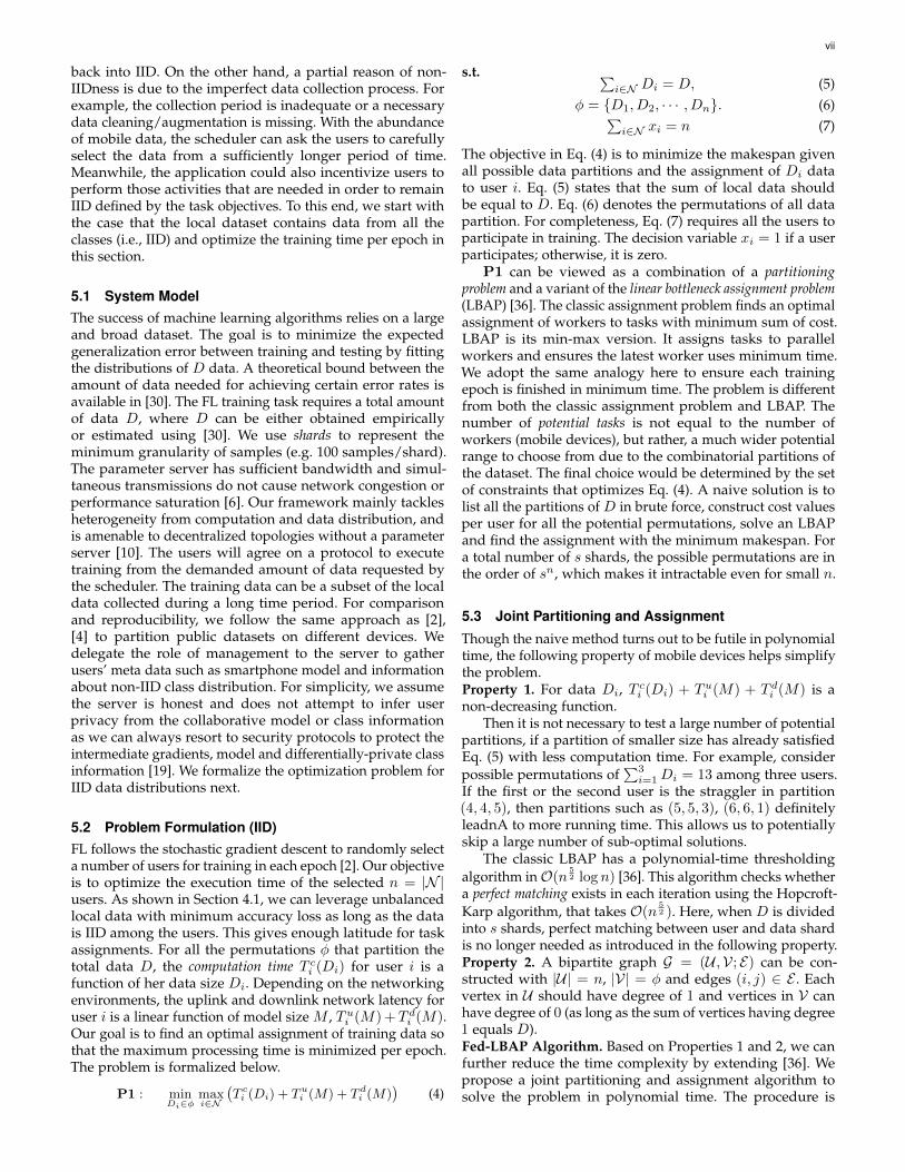
Experiment Setting. We use the collection of devices toconstruct five combinations of mobile testbeds as shown inTable 2. The experiment is conducted on two commonlyused datasets: MNIST [41] and CIFAR10 [42] with 60Kand 50K training samples. We fully charge all the devices,pre-load both datasets into the mobile flash storage andread them in mini-batches of 20 samples. Users perform

xi

model SoC CPU big.LITTLENexus 6 Snapdragon 805 4×2.7GHz 7

Nexus 6P Snapdragon 810 4×1.55 GHz4×2.0 GHz 3

Samsung J8 Snapdragon 450 8×1.8GHz 7

Mate 10 Kirin 970 4×2.36GHz4×1.8GHz 3

Pixel2 Snapdragon 835 4×2.35 GHz4×1.9 GHz 3

P30 Pro Kirin 9802×2.6 GHz2×1.92 GHz4×1.8 GHz

3

TABLE 1: Hardware configurations of benchmarking testbed.

N6 N6P J8 Mate10 Pixel2 P30 TotalT1 1 - - 1 1 - 3T2 2 2 - 1 1 - 6T3 4 2 - 2 2 - 10T4 6 2 1 2 2 1 14T5 8 3 2 2 3 2 20

TABLE 2: Experimental mobile testbedsone epoch of local training in each round and the globalgradient averaging iterates 50 and 100 epoches for MNISTand CIFAR10 respectively.

To emulate the dynamics of mobile data, we generaterandom distributions among the users: 1) For IID data, eachuser retains all the classes and the ratio between samplesfrom different classes is equivalent; 2) For non-IID data,each user has a random subset of classes and each classmay also have different number of samples. We set themaximum number of classes in the subset to 7 (out of thetotal 10 classes), i.e., on average, a user would have about3.5 classes. The purpose is to see whether our algorithmcan handle various random cases of non-IID distributions.Two fundamental networks of LeNet [38] and VGG6 [39]are evaluated and their efficiency has been proved to handlelearning problems at sufficient scales. To meet the inputdimensions, we tailor the original 16 layers of VGG16 bystacking five 3 × 3 convolutional layers with one denselyconnected layer. We set parameter α in Mincost to 1.8and 2.45 for LeNet and VGG6 empirically as discussed inSection 8.5. The uplink and downlink latencies are added tocomputation time.

Benchmarks. The proposed algorithms are comparedwith several benchmarks: 1) Proportional: a simple heuristicthat assigns training data proportional to the processingpower of mobile devices statically measured by their maxCPU frequencies; 2) Random: random data partitions amongthe users; 3) FedAvg [2]: assign equal shares of data to users.Since the model architecture is fixed, we mainly compare thecomputational time and treat the communication time as aconstant. To facilitate the evaluation, we also adopt pytorchwith GTX1080/K40 GPUs to evaluate different benchmarks.

8.1 Profiling PerformanceAs the basis to launch optimization, we evaluate the ef-fectiveness of the profiling method in Sec. 7. We learn theregressor on 25 neural networks and test on 8 networks withparameters ranging from 0.2M to 12M. Recall that in thefirst step, we model the relation between the parametersand training time. Some results are shown in Fig.9. We cansee that the slope of the hyperplane of Nexus6 is steeper

6

4

106

# of param. (Dense Layer)

Regression of compute time (Nexus6 vs. Mate10)

020

2000

0.5

105

# of param. (Conv Layer)

1 1.5

4000

Com

pute

Tim

e (

s)

2 2.5 03

6000

3.5

8000

Nexus6

Mate10

Fig. 9: Step 1, profile trainingtime with model parameters.

Device [α0, α1, α2]Nexus6 [578, 0.02, 2e-5]

Nexus6P [647, 8e-3, 3e-4]SJ8 [183, 1e-2, 9e-5]

Mate10 [47, 2e-3, 2e-5]Pixel 2 [68, 2e-3, 1e-5]

P30 [42, 2e-3, 1e-5]

TABLE 3: Learned parameters(Eq. 17): α0, intercept; α1, conv.layer; α2, dense layer.

0 10 20 30 40 50 60

Training data (# of data batch)

0

500

1000

1500

2000

2500

3000

3500

4000

Tim

e (

s)

Step 2: Compute time vs. data size (batches)

Estimation (Nexus 6)

Actual Measurement(Nexus 6)

Estimation (Mate10)

Actual Measurement(Mate10)

Nexus 6

P30

(a)

105 106 107 108

# of Parameters

10-1

100

101

102

RM

SE

Profiling error on test set

Nexus6

Nexus6PSamsungJ8Mate10Pixel2P30

Higher RMSE

(b)

Fig. 10: Step 2: predict training time vs. data size. a) Nexus 6vs. P30; b) profiling error on test set.

than Mate10, representing more computational time fromthe older smartphone generations. The upward trend ismore pronounced in the convolutions and this validatesthe operation to separate convolution from the dense layers.Table 3 shows the learned parameters by the linear regressionmodel. The values α1, α2 directly associate with the compu-tational capabilities in conducting matrix multiplications forthe convolution and dense layers. A larger value indicatesless computational power and the ranking order is consistentwith the rest experiments.

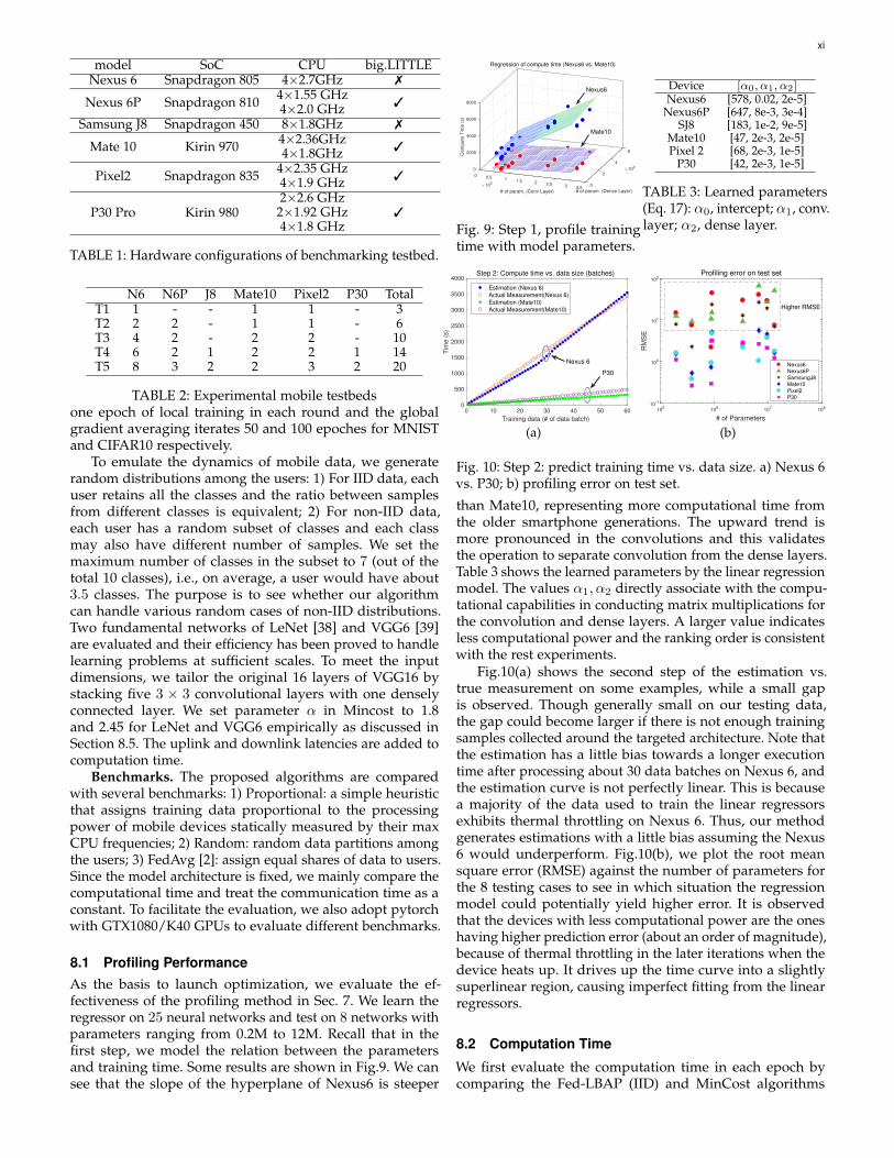
Fig.10(a) shows the second step of the estimation vs.true measurement on some examples, while a small gapis observed. Though generally small on our testing data,the gap could become larger if there is not enough trainingsamples collected around the targeted architecture. Note thatthe estimation has a little bias towards a longer executiontime after processing about 30 data batches on Nexus 6, andthe estimation curve is not perfectly linear. This is becausea majority of the data used to train the linear regressorsexhibits thermal throttling on Nexus 6. Thus, our methodgenerates estimations with a little bias assuming the Nexus6 would underperform. Fig.10(b), we plot the root meansquare error (RMSE) against the number of parameters forthe 8 testing cases to see in which situation the regressionmodel could potentially yield higher error. It is observedthat the devices with less computational power are the oneshaving higher prediction error (about an order of magnitude),because of thermal throttling in the later iterations when thedevice heats up. It drives up the time curve into a slightlysuperlinear region, causing imperfect fitting from the linearregressors.

8.2 Computation Time

We first evaluate the computation time in each epoch bycomparing the Fed-LBAP (IID) and MinCost algorithms

xiiTraining time (MNIST-LeNet)

T1 T2 T3 T4 T5

Testbed

101

102

103

104

Tim

e p

er

glo

ba

l u

pd

ate

(s)

Random

Prop.

FedAvg

LBAP-IID

Mincost-NonIID

(a)

Training time (MNIST-VGG6)

T1 T2 T3 T4 T5

Testbed

102

103

104

105

Tim

e p

er

glo

ba

l u

pd

ate

(s)

Random

Prop.

FedAvg

LBAP-IID

Mincost-NonIID

(b)

Training time (CIFAR10-LeNet)

T1 T2 T3 T4 T5

Testbed

101

102

103

Tim

e p

er

glo

ba

l u

pd

ate

(s)

Random

Prop.

FedAvg

LBAP-IID

Mincost-NonIID

(c)

Training time (CIFAR10-VGG6)

T1 T2 T3 T4 T5

Testbed

102

103

104

Tim

e p

er

glo

ba

l u

pd

ate

(s)

Random

Prop.

FedAvg

LBAP-IID

Mincost-NonIID

(d)Fig. 11: Comparison of computation time when data is IID (time in log-scale) (a) training MNIST with LeNet; (b) trainingMNIST with VGG6; (c) training CIFAR10 with LeNet; (d) training CIFAR10 with VGG6.

Different schemes (MNIST)

Prop.

Ran

dom

FedAvg

BLAP

0.98

0.985

0.99

0.995

1

acc.

LeNet

VGG6

Different schemes (CIFAR10)

Prop.

Ran

dom

FedAvg

BLAP

0

0.2

0.4

0.6

0.8

acc.

LeNet

VGG6

T1 T2 T3 T4 T50.98

0.985

0.99

0.995

acc.

Different testbeds (MNIST)

LeNet

VGG6

T1 T2 T3 T4 T50.5

0.6

0.7

0.8

acc.

Different testbeds (CIFAR10)

LeNet

VGG6

Fig. 12: Comparison of accuracy across different schemes andtestbeds (IID).

(Non-IID) with the benchmarks shown in Fig. 11. Weenumerate all the combinations between the testbed, datasetsand models. Fed-LBAP achieves the lowest computationaltime with 2× to 100× speedup compared to the benchmarks(time-optimal). Mincost adjusts the workload assignmentbased on the Non-IID distributions to trade epoch-wisecomputation time for faster convergence, which requires5-10% time in most cases.

By taking a closer look of the testbed devices, we cansee that the mobile processing power (both individualand collective) and their workloads play key roles in thecomputational time, which sum up to nontrivial relations.First, unlike cloud settings in which computation time scaleswell with the number of workers, mobile stragglers easilyslows down the entire training even if more users areinvolved: the time surge from T1 (3 users) to T2 (6 users)is due to the addition of Nexus6P, impacted by the severethermal throttling. This drag is magnified with complexnetwork architectures of higher computation intensity (VGG6with more convolutional layers) and more training data (60Kof MNIST vs. 50K CIFAR10). The shares from the 10K dataaddition exacerbate the computation time parabolically by20 times (T2 between Figs. 11(b) and (d) running VGG6 onMNIST and CIFAR10), if the scheduling is done inappropri-ately. Bringing more devices could ease up the bottleneck asthe time declines from T3 to T5 with more participants.

Using the vanilla schemes (Prop., Random and FedAvg),we hardly see any consistent parallelism when more users areinvolved, where the stragglers defeat the original purpose ofdistributed learning. In contrast, Fed-LBAP and Mincost are

capable of utilizing the additive computational resources byappropriately assigning workloads to the more efficient users,so the training time accomplishes a downtrend with moreusers, even when the worst-case stragglers are present. Thisis because the proposed algorithms can purposely assign datain proportion to the device’s capacity, once the thermal effectshave been quantified. Although naive schemes may look foran optimal scheduling that is proportional to device CPUfrequency or equally assign workloads as [2], the runtimebehavior may be drastically different due to complex systemdynamics, and our experiment shows that such schemesare on par with a purely random schedule. Note that weonly perform one local epoch in each iteration. More localepoches can accelerate global convergence [2]. Our strategyis invariant to the upper-layer learning algorithms and thetime saving would be indeed much higher if more than onelocal epoches are performed.

8.3 Accuracy

It is essential to evaluate the test accuracy after workloadre-assignment, especially our efforts to improve accuracy incase of non-IID data. Fig. 12 summarizes the test accuracyunder different scheduling schemes and testbeds when datais IID. The two upper plots compare the average accuracy ofFed-LBAP with the benchmarks. Our findings in the large-scale experiment are consistent with the previous motivationdiscovery, which drives the design of Fed-LBAP. For IID data,even random assignments do not have accuracy loss. SinceFed-LBAP can be considered as one special permutationfrom the random partitions, the results indicate that we canalways leverage load unbalancing to optimize computation timewithout worrying about accuracy loss, if user data is IID. The twolower plots show that accuracy trends down (with LeNet)when more users are involved (from 3 to 20 users). Theobservation is inline with [2] and suggests an inherent trade-off between parallelism and global convergence, which isfurthered discussed in the next subsection.

Fig. 13 compares Mincost with the benchmarks when datais Non-IID. We vary the random seeds to generate differentclass distributions, i.e., each user has a random subsetfrom all the classes. Each point in the figure correspondsto an accuracy measurement. Mincost surpasses all thebenchmarks by 0.02 in MNIST and 0.04 in CIFAR (2-7%increase in accuracy), including the Fed-LBAP algorithmwhich we directly apply on the Non-IID data. This justifiesthe introduction of accuracy cost in Mincost − though usingFed-LBAP for non-IID data is time-optimal, its accuracy ison the same level of the benchmarks. It is interesting tosee that the accuracy actually climbs up with more users

xiii

T1 T2 T3 T4 T5

0.6

0.7

0.8

0.9

1

Accu

racy

Non-IID Accuracy (MNIST-LeNet)

Prop.

Random

FedAvg

LBAP

MinCost

(a)T1 T2 T3 T4 T5

0.65

0.7

0.75

0.8

0.85

0.9

0.95

1

Accu

racy

Non-IID Accuracy (MNIST-VGG)

Prop.

Random

FedAvg

LBAP

MinCost

(b)T1 T2 T3 T4 T5

0.25

0.3

0.35

0.4

0.45

0.5

0.55

0.6

Accu

racy

Non-IID Accuracy (CIFAR-LeNet)

Prop.

Random

FedAvg

LBAP

MinCost

(c)T1 T2 T3 T4 T5

0.3

0.4

0.5

0.6

0.7

Accu

racy

Non-IID Accuracy (CIFAR-VGG)

Prop.

Random

FedAvg

LBAP

MinCost

(d)Fig. 13: Comparison of accuracy (Non-IID) (a) MNIST-LeNet; (b) MNIST-VGG6; (c) CIFAR10-LeNet; (d) CIFAR10-VGG6.

0 10 20 30 40 50

Epoches

0.3

0.4

0.5

0.6

0.7

0.8

0.9

1

Accu

racy

0

200

400

600

800

Co

mp

uta

tio

n T

ime

(s)

Convergence time (MNIST-LeNet-T3)

FedAvg

Fed-LBAP

Mincost

Accuracy

Comp. Time

(a)

0 10 20 30 40 50

Epoches

0.4

0.5

0.6

0.7

0.8

0.9

1

Accu

racy

0

2000

4000

6000

8000

10000

Co

mp

uta

tio

n T

ime

(s)

Convergence time (MNIST-VGG-T4)

FedAvg

Fed-LBAP

Mincost

Accuracy

Comp. Time

(b)

0 10 20 30 40 50

Epoches

0.1

0.15

0.2

0.25

0.3

0.35

0.4

Accu

racy

0

100

200

300

400

500

600

700

Co

mp

uta

tio

n T

ime

(m

in)

Convergence time (CIFAR10-LeNet-T2)

FedAvg

Fed-LBAP

Mincost

Accuracy

Comp. Time

(c)

0 10 20 30 40 50

Epoches

0.1

0.2

0.3

0.4

0.5

0.6

0.7

0.8

Accu

racy

0

200

400

600

800

1000

1200

Co

mp

uta

tio

n T

ime

(m

in)

Convergence time (CIFAR10-VGG-T5)

FedAvg

Fed-LBAP

Mincost

Accuracy

Comp. Time

(d)Fig. 14: Comparison of total convergence time (a) MNIST-LeNet-T3 (10 users) (b) MNIST-VGG6-T4 (14 users); (c) CIFAR10-LeNet-T2 (6 users); (d) CIFAR10-VGG6-T5 (20 users).

in Non-IID data, where the opposite is perceived in Fig.12 with IID data. This is because more users increase theclass coverage of the population. Mincost can utilize thesedynamics from more dispersed class distributions, and selectthe participants wisely to either avoid or retain those n-class outliers (where n = 1 − 2 in our experiment). Hence,the accuracy improvement is significant with more users,especially on more complex dataset as CIFAR10.

8.4 Convergence TimeThe Mincost algorithm trades the computational time perepoch over the long-term convergence time. We evaluatethe effectiveness of such trade-off by comparing to thetime-optimal Fed-LBAP and the vanilla FedAvg. The goalis to compare the total time in order to achieve 95%accuracy among the weakest of FedAvg, Fed-LBAP andMincost, which is either FedAvg or Fed-LBAP accordingto the previous accuracy evaluation. We select a case ineach dataset-network combination and plot accuracy andcomputational time in two y-axis with the training epocheson the x-axis of Fig. 14. The results are averaged over10 different random class distributions among the users.Network communication time to upload/download modelis added to the computation time, so it represents the entireduration of each global update. The convergence time isobtained by connecting the accuracy goal on the left y-axisto the accumulated computation time on the right y-axis.

Mincost offers much faster convergence - about halfnumber of epoches to achieve the same level of accuracy.However, for the entire duration, only if the time savings fromfaster convergence surpasses the extra time spent in each epoch,Mincost could outperform Fed-LBAP in Non-IID data. Beforewe see the results, let us derive this relation analytically.The convergence curve of the i-th neural network can bemodeled by an exponential function pi(x) = Ai − e−βix. xis the number of epoches. pi(x) is the prediction accuracyafter x epoches. Ai is the best accuracy the network couldachieve empirically. βi reflects the convergence rate. Oncethe computational time is known per epoch, the total timecan be represented by a linear function ki · x corresponding

50 100 150 200 250 300 350

Computation Time ( =0.6-3.4)

0.8

0.85

0.9

0.95

1

Accura

cy

Computation time vs. accuracy (MNIST-LeNet)

Avg. accuracy

Trendline

optimal selecting range

(a)

500 1000 1500 2000

Computation Time ( =1.25-3.45)

0.52

0.54

0.56

0.58

0.6

0.62

0.64

0.66

Accura

cy

Computation time vs. accuracy (CIFAR10-VGG)

Avg. accuracy

Trendline

optimal selecting range

(b)

Fig. 15: Relations between computation time and accuracywith different parameter α. a) MNIST-LeNet b) CIFAR10-VGG6. (Colored dots represent different non-IID distribu-tions generated from different random seeds).

to the y-axis on the R.H.S. in Fig. 14. The condition for thecompuational time of Mincost (k1x1) to be less than Fed-LBAP (k2x2) is,

k1x1 < k2x2

1

β1log(A1 − p)k1 <

1

β2log(A2 − p)k2

p <eβ1k2A2 − eβ2k1A1

eβ1k2 − eβ2k1(18)

The relation indicates that Mincost outperforms Fed-LBAPwhen the goal of accuracy is upper-bounded by Eq. (18).It echoes with our observations in Fig. 14 that trainingprogresses much faster with Mincost at the beginning. Itprovides 1.5 − 1.8× and a tremendous 7 − 200× speed-up compared to Fed-LBAP and FedAvg respectively. Theexperiment ultimately justifies our design of accuracy cost oncarefully selecting the participants and assigning workloadsbased the class distributions. Compared to our previouswork [44], which strives to preserve accuracy without loss,we not only improve the testing accuracy, but also the overallcomputational time.

xiv

8.5 Selection of Parameter αThere is still an important hyperparameter left to explainin Mincost - the scaling parameter α that balances theaccuracy cost and computation time. We seek answers tothe fundamental question: whether there exists an optimalα that can minimize the total computation time and howits value drives the process of decision making? Fig. 15partially answers the optimality question by enumerating itsvalue from 0.6 − 3.4 for MNIST-LeNet and 1.25 − 3.45 forCIFAR10-VGG6. For clarity, we present 6 random non-IIDdistributions (represented by the dots in different colors)and their average accuracy vs. computation time. Thecomputation time is monotonically increasing as α grows,because Mincost deviates from Fed-LBAP to favor thoseusers with less accuracy cost (more num. of classes). Theyare most likely less time-optimal. An extreme case is whenNexus 6P device has all the classes, whereas the rest usersonly have a few classes. A large α assigns more data to thestraggler and makes the time cost higher.

Despite its monotonicity with computation time, theimplication on accuracy is not straightforward as the rela-tionship is highly nonconvex. As seen in Fig. 15, the averageaccuracy trends up initially and drops promptly. We utilize aquadratic least square fitting to characterize both trendlines.However, the individual accuracy-vs-computation may notalways hold such parabolic shape. The general downtrendis still intact as we increase α (and in turn computationtime). This is because as α goes up, Mincost merely assignsworkloads to those users with more classes and leavesthe rest vacant. Of course, it undermines parallelism offederated learning and elongates computation time. Theredoes exist a “sweet spot” for choosing α as the highlightedregion, in which a mild increase of computation time canbe compensated by the faster convergence as demonstratedpreviously.

8.6 Performance Gap due to Profiling ErrorFinally, we evaluate possible performance gaps due totwo types of imperfections in profiling. Type I: if the run-time trace is available from Step 1 in Fig. 9, the secondstep with least square estimation incurs some minor gapsshown in Fig. 10(a); Type II: for untested architectures (run-time trace unavailable from Step 1), using the number ofparameters for prediction brings more uncertainties. ForType I error, we measure the performance gaps betweenthe real measurement, “Real”, and the least square estimate,“Estimate” in Fig. 16. The result shows the time differenceinduced by the inaccurate profile while running Fed-LBAPand Mincost. The estimation error is within 5% for most casesand at most 25% for some cases in MNIST. We scrutinizethe data assignments and find that they are almost the same.Thus, there is no visible accuracy loss due to Type I error.

There are often cases that a new network architecture isimplemented and the profiling data has not been collectedyet. Our best shot is to use the known profiles to predictthe computation time on a target mobile device given thenumber of model parameters (from convolutional and denselayers separately) and the amount of training data. Fig.10(b) indicates that the prediction RMSE is nonzero andthe estimation error is accumulated in the later epoches.We construct a new testbed with 6 devices (one from each

T1 T2 T3 T4 T5

Testbed

0

50

100

150

200

Tim

e p

er

glo

bal update

(s)

Imperfection due to Type I error (MNIST-LeNet)

Real-IID

Estimate-IID

Real-NonIID

Estimate-NonIID

(a)

Imperfection due to Type I error (CIFAR10-VGG)

T1 T2 T3 T4 T5

Testbed

0

500

1000

1500

2000

Tim

e p

er

glo

bal update

(s)

Real-IID

Estimate-IID

Real-NonIID

Estimate-NonIID

(b)

Fig. 16: Performance gaps due to Type I error a) MNIST-LeNet b) CIFAR10-VGG.

smartphone model) and utilize the 8 testing architectures.As seen in Fig. 17(a), the error is much larger than Type I.A common error we found is caused by overestimating therunning time of some devices, which causes the algorithmto miscalculate (reduce the data assignment but increase forothers. For example, we found that sometimes the Nexus6Ptraining time is mistakenly doubled by the estimation andthe algorithm assigns more data to the rest devices, whichcould have been run on Nexus6P without severe throttling.A partial reason is due to the limitations of the linear modelswhen some devices actually exhibit nonlinear behaviors underdifferent computational intensity.

We conduct more experiments to see the impact onconvergence in Fig. 17(b). The curve is the averaged accuracyover all 8 datasets by enumerating 10 different non-IIDclass distributions. Fortunately, unlike the timing gap, bothcurves converge to almost the same accuracy. However, theestimation has about 1-2 epoches latency, which amounts to10-20 mins using only 6 devices. With more devices, suchslowdown can be amortized effectively. As a result, themajor instability mainly comes from modeling an untestedarchitecture, when any under/overestimations would leadto sub-optimal assignment.

73 86 90 177 181 309 351 442

Testset (~K parameters)

0

500

1000

1500

2000

2500

3000

Tim

e p

er

glo

bal update

(s)

Imperfection due to Type II error (MNIST)

Real-IID

Estimate-IID

Real-NonIID

Estimate-NonIID

max. 40-50% delay

(a)

0 10 20 30 40 50

Epoches

30

40

50

60

70

80

90

Accura

cy

Impact of Type II error on convergence (MNIST)

Real-NonIID

Estimate-NonIID

(b)

Fig. 17: Performance gaps due to Type II error a) MNIST-LeNet b) CIFAR10-VGG.

9 DISCUSSION

The proposed framework utilizes linear regression to profilethe training time on different devices. For federated tasks, themodels are usually known beforehand, with necessary archi-tectural adaptations to add/remove filters and adjust layerscommensurate to the input dimension and memory limit. Inthis paper, we estimate the training time of specific modelarchitectures related to the size of training data. Althoughour evaluations are based on the networks in the VGG family,

xv

the method is applicable to the more complex ConvolutionalNeural Networks (CNN) and Recurrent Neural Networks(RNN) such as the ResNet [46], Inception-ResNet [47] andLong Short Term Memory (LSTM) networks [48].

Modern neural architectures are designed with complexlayer dependencies and irregular dataflow, that lead to moretime in memory access [49]. For example, the ResNet utilizesbypass links to facilitate gradient flow and the Inceptionmodules [47] merge multiple branches. In principle, compu-tation in neural networks is dominated by the number ofmultiply-add, e.g., from the convolutional and fully connectedlayers. It can be efficiently estimated using the number ofFloating Point Operations (FLOPs)/model parameters. Forthe same type of networks, the linear relation generally holdsbecause the number of FLOPs is proportional to the amountof training time when the computing resources are fullyutilized on mobile. The time spent during memory accessalso remains proportionally similar. We have conductedmore experiments to execute training of ResNet and LSTMin our testbed as discussed below. For LSTM, we use thedataset from the Physionet Challenge [51], which consists of4000 patients ICU visits of 86 feature vectors and a binarymortality label. We take 4% of the data to train: i) a one-layerLSTM network with 300 units; ii) a two-layer LSTM networkwith 300 units in each layer.

Fig. 18 plots the training time vs. the number of modelparameters of ResNet architectures by adding/removingconvolutional layers, adjusting kernel size and number offilters (on the two representative lowgrade devices). Wecan see that the linear relation generally holds. Note thatadding/removing convolutional layers may have resultedsimilar number of parameters with adjusting the number offilters, but their training time may have noticeable difference,i.e., adding a convolutional layer typically leads to moretraining time due to increased cross-layer memory access.We have also tested Inception-ResNet and LSTM and theirresults reveal similar linearity relations. Next, we confirmthat the linear relation also holds between the trainingtime vs. the number of data batches in LSTM networkas shown in Fig. 19. Some interesting phenomenons alsoworth discussion: 1) the execution time is much longerthan the CNN with similar number of parameters. Thisis consistent with training LSTM on cloud GPU as it hasvery different dataflow/computation patterns from the CNN.2) The memory demand is much higher per data batch. Ittriggers the background Garbage Collection activities quiteoften, which pause the training threads multiple times perepoch to free memory. Thus, in addition to the increasedtime, there are noticeable fluctuations on both curves.

On the positive side, the CPU can take a breath duringmemory free and the time spent in memory access. This isvalidated in Fig. 20 that we show the trace of two devicesthat are prone to thermal throttling. For Nexus 6, if wecompare the increase of temperature in Figs. 3(a-b) with Fig.20, the temperature curve of LSTM on Nexus6 obviouslyclimbs much slower than training the CNN, thus creatingmore opportunities to run at high clockspeed; in contrast,the Nexus 6P still keeps shutting down the big cores tomaintain their temperature below 55 degrees, which is moreconservative compared to its predecessor.

For the non-IID properties discovered in this paper,they stem from the basic principles of deep learning which

should also hold for both CNN and RNN networks. That is,high class imbalance, missing categorical information leadto accuracy loss and unseen samples help generalize themodel. Due to space limit, we do not include a thoroughevaluation, but the proposed mechanism is model-agnosticand applicable to a wide range of mobile devices on themarket.

0 100 200 300 400 500

# of Model Parameters (K)

100

150

200

250

300

Tra

inin

g T

ime (

10 e

poches)

Profile training time of ResNet (Nexus6)

Measurement

Linear Regression

(a)

0 100 200 300 400 500

# of Model Parameters (K)

80

100

120

140

160

180

200

Tra

inin

g T

ime

Profile training time of ResNet (Nexus6P)

Measurements

Linear Regression

(b)

Fig. 18: Profile ResNet architectures on the Nexus 6/6P.

2 4 6 8 10

Data Batch (Size=8)

0

100

200

300

400

500

Tra

inin

g T

ime (

s)

Profiling training time of LSTM (1 layer,300 units)

Nexus6

Nexus6P

SamsungJ8

Mate10

Pixel2

P30

(a)

2 4 6 8 10

Data Batch (Size=8)

0

200

400

600

800

1000

Tra

inin

g T

ime (

s)

Profiling training time of LSTM (2 layers,600 units)

Nexus6

Nexus6P

SamsungJ8

Mate10

Pixel2

P30

(b)

Fig. 19: Profiling LSTM training time. (a) Layer-LSTM, 300units (b) 2 Layer-LSTM, 600 units.

1 2 3 4 5 6 7 8 9 10

Data batch (8 samples/batch)

2.45

2.5

2.55

2.6

2.65

Fre

q.

(GH

z)

Nexus6: CPU Frequency (LSTM)

1 2 3 4 5 6 7 8 9 10

Data batch (8 samples/batch)

50

60

70

80

Te

mp

. (C

els

ius)

Nexus6: Temperature (LSTM)

(a)

1 2 3 4 5 6 7 8 9 10

Data batch (8 samples/batch)

0

0.5

1

1.5

2

Fre

q.

(GH

z)

Nexus6P: CPU Frequency (LSTM)

Small Cluster

Big Cluster

1 2 3 4 5 6 7 8 9 10

Data batch (8 samples/batch)

50

55

60

65

Te

mp

. (C

els

ius)

Nexus6P: Temperature (LSTM)

Small Cluster

Big Cluster

(b)

Fig. 20: Profiling CPU frequency vs. temperature. (a) Nexus6, (b) Nexus 6P.

10 CONCLUSION

In this paper, we study efficient scheduling of federatedmobile devices under both device and data-level heterogene-ity. We motivate this work by showing drastically differentprocessing time under the same workload and opportuni-ties to employ user selection to improve non-IID learningaccuracy. We develop two efficient near-optimal algorithmsto schedule workload assignments for both IID and non-IID data, and visualize the solution space analytically. Ourextensive experiments on real mobile testbed and datasets

xvi

demonstrate up to 2 orders of magnitude speedups anda moderate accuracy boost when data is non-IID. We alsodemonstrate cases when our algorithm deviates from theoptimal region due to estimation gaps in the profilingprocess.

ACKNOWLEDGMENTS

This work was supported in part by the US NSF grantnumbers CCF-1850045, IIS-2007386 and the State of VirginiaCommonwealth Cyber Initiative (cyberinitiative.org).

REFERENCES

[1] J. Dean, et. al., “Large scale distributed deep networks”,NIPS, 2012.

[2] B. McMahan, E. Moore, D. Ramage, S. Hampson, B. Ar-cas, “Communication-efficient learning of deep networksfrom decentralized data”, AISTATS, 2017.

[3] X. Li, K. Huang, W. Yang, S. Wang and Z. Zhang, “Onthe convergence of FedAvg on Non-IID Data”, ICLR,2020.

[4] Y. Zhao, M. Li, L. Lai, N. Suda, D. Civin and V.Chandra, “Federated Learning with Non-IID Data”,arXiv:1806.00582.

[5] E. Jeong, S. Oh, H. Kim, S. Kim, J. Park and M. Bennis,“Communication-efficient on-device machine learning:federated distillation and augmentation under non-IIDprivate data”, NIPS-MLPCD, 2018.

[6] K. Bonawitz, et. al., “Towards federated learning at scale:system design”,SysML Conference, 2019.

[7] Y. Chen, S. Biookaghazadeh, and M. Zhao, “Exploringthe Capabilities of Mobile Devices in Supporting DeepLearning”, ACM/IEEE Symposium on Edge Computing,2019.

[8] J. Konecny, et. al., “Federated learning: strategies forimproving communication efficiency”,NIPS, 2016.

[9] L. Wang, W. Wang and B. Li, “CMFL: Mitigating commu-nication overhead for federated learning”, IEEE ICDCS,2019.

[10] X. Lian, et. al., “Can decentralized algorithms outper-form centralized algorithms? A case study for decentral-ized parallel stochastic gradient descent”, NIPS, 2017.

[11] H. Zhu, Y. Jin,“Multi-objective evolutionary federatedlearning”,arXiv preprint arXiv:1812.07478, 2018.

[12] V. Smith, C. Chiang, M. Sanjabi and A. Talwalkar,“Federated multi-task learning”, NIPS, 2017.

[13] L. Liu, J. Zhang, S. H. Song, K. Letaief, “Client-Edge-Cloud hierarchical federated learning”,arXiv: 1905.06641,2019.

[14] S. Zheng, Q. Meng, T. Wang, W. Chen, N. Yu, Z. Ma andT. Liu, “Asynchronous stochastic gradient descent withdelay compensation”, ICML, 2017.

[15] Q. Ho, J. Cipar, H. Cui, J. Kim, S. Lee, P. Gibbons, G. Gib-son, G. Ganger and E. Xing, “More effective distributedML via a stale synchronous parallel parameter server”,NIPS, 2013.

[16] J. Vicarte, B. Schriber, R. Paccagnella and C. Fletcher,“Game of Threads: Enabling Asynchronous PoisoningAttacks”, ACM ASPLOS, 2020.

[17] R. Tandon, Q. Lei, A. Dimakis and N. Karampatziakis,“Gradient coding,” NIPS, 2016.

[18] B. McMahan and D. Ramage, “Federated Learning:Collaborative Machine Learning without CentralizedTraining Data”, Google AI Blog, 2017.

[19] K. Bonawitz, et. al., “Practical secure aggregation forprivacy-preserving machine learning”, ACM CCS, 2017.

[20] P. Blanchard, E. Mhamdi, R. Guerraoui and J. Stainer,“Machine learning with adversaries: byzantine tolerantgradient descent”, NIPS, 2017.

[21] Apple A13 Bionic chip,https://www.macworld.com/article/3442716/inside-apples-a13-bionic-system-on-chip.html.

[22] Huawei kirin 980 AI chip,https://consumer.huawei.com/en/campaign/kirin980/.

[23] X. Zeng X, K. Cao, M. Zhang,“MobileDeepPill: A small-footprint mobile deep learning system for recognizingunconstrained pill images”, ACM Mobisys, 2017.

[24] A. Mathur, N. Lane, D. Bhattacharya, S. Boran, A.Forlivesi, C. Kawsar, “Deepeye: Resource efficient localexecution of multiple deep vision models using wearablecommodity hardware”, ACM Mobisys, 2017.

[25] S. Han, H. Mao and W. J. Dally, “Deep compression:compressing deep neural networks with pruning, trainedquantization and huffman coding”, ICLR, 2016.

[26] J. Frankle and M. Carbin, “The lottery ticket hypothesis:finding sparse, trainable neural networks”, ICLR, 2019.

[27] C. Wang, Y. Xiao, X. Gao, L. Li and J. Wang, “Close thegap between deep learning and mobile intelligence byincorporating training in the loop”, ACM Multimedia,2019.

[28] ARM’s big.LITTLE, https://www.arm.com/why-arm/technologies/big-little

[29] Android large heap, https://developer.android.com/guide/topics/manifest/application-element

[30] D. Haussler, “Quantifying inductive bias: AI learningalgorithms and Valiant’s learning framework,” Journal ofArtif. Intell., vol. 36, no. 2, pp. 177-221, 1988.

[31] L Epstein and J. Sgall, “Approximation Schemes forScheduling on Uniformly Related and Identical ParallelMachines”, ESA, pp. 151-162, 1999.

[32] Y. Peng, Y. Bao, Y. Chen, C. Wu and C. Guo, “Opti-mus: an efficient dynamic resource scheduler for deeplearning clusters”, EuroSys, 2018.

[33] Y. Bao, Y. Peng, C. Wu and Z. Li,“Online Job Schedul-ing in Distributed Machine Learning Clusters”, IEEEINFOCOM, 2018.

[34] D. Yin, A. Pananjady, M. Lam, D. Papailiopoulos, K.Ramchandran and P. Bartlett, “Gradient diversity: a keyingredient for scalable distributed learning”, AISTATS,2018.

[35] In-depth with the Snapdragon 810’s heat prob-lems, https://arstechnica.com/gadgets/2015/04/in-depth-with-the-snapdragon-810s-heat-problems

[36] R. Burkard, M. Dell’Amico and S. Martello, “Assign-ment problems”, SIAM, 2012

[37] J. B. Mazzola and A. W. Neebe, “Bottleneck generalizedassignment problems”, Engineering Costs and ProductionEconomics, vol. 14, no. 1, pp. 61-65, 1988.

[38] Y. Lecun, L. Bottou, Y. Bengio and P. Haffner, “Gradient-based learning applied to document recognition”, inProceedings of the IEEE, vol. 86, no. 11, pp. 2278-2324,Nov. 1998.

xvii

[39] K. Simonyan and A. Zisserman, “Very deep convolu-tional networks for large-scale image recognition”, ICLR,2015.

[40] B. LeCun, T. Mautor, F. Quessette and M. Weisser,“Bin packing with fragmentable items: Presentation andapproximations”, Theo. Comp. Sci., vol. 602, 2015.

[41] MNIST dataset, http://yann.lecun.com/exdb/mnist/[42] CIFAR10 dataset,

https://www.cs.toronto.edu/ kriz/cifar.html[43] Deep Learning for Java, https://deeplearning4j.org[44] C. Wang, X. Wei and P. Zhou, “Optimize scheduling of

federated learning on battery-powered mobile devices”,IEEE IPDPS, 2020.

[45] F. Iandola, S. Han, M. W. Moskewicz, K. Ashraf, W. Dallyand Kurt Keutzer, “SqueezeNet: AlexNet-level accuracywith 50× fewer parameters and <0.5MB model size”,ICLR, 2017.

[46] K. He, X. Zhang, S. Ren and J. Sun, “Deep ResidualLearning for Image Recognition,” IEEE CVPR, 2016.

[47] C. Szegedy, S. Ioffe, V. Vanhoucke and A. A. Alemi,“Inception-v4, Inception-ResNet and the Impact of Resid-ual Connections on Learning”, AAAI, 2017.

[48] S. Hochreiter and J. Schmidhuber, “Long short-termmemory,” Neural Computation, vol. 9, no. 8, pp. 17351780,1997.

[49] W. Jung, D. Jung, B. Kim, S. Lee, W. Rhee and J. H. Ahn,“Restructuring Batch Normalization to Accelerate CNNTraining”, SysML, 2019.

[50] C. Wu, et. al, “Machine Learning at Facebook: Un-derstanding Inference at the Edge,” IEEE InternationalSymposium on High Performance Computer Architecture(HPCA), 2019

[51] Physionet Challenge,https://physionet.org/content/challenge-2012/1.0.0

Cong Wang received the B. Eng degree in Infor-mation Engineering from the Chinese Universityof Hong Kong in 2008, M.S. degree in ElectricalEngineering from Columbia University in 2009,and Ph.D. in Computer and Electrical Engineeringfrom Stony Brook University, NY, in 2016. He iscurrently an Assistant Professor at the ComputerScience department, Old Dominion University,Norfolk, VA. His research focuses on exploringalgorithmic solutions to address security and pri-vacy challenges in Mobile, Cloud Computing, IoT,

Machine Learning and System. He is the recipient of the CommonwealthCyber Initiative Research and Innovation Award, ODU Richard ChengInnovative Research Award and IEEE PERCOM Mark Weiser Best PaperAward in 2018.

Yuanyuan Yang received the BEng and MSdegrees in computer science and engineeringfrom Tsinghua University, Beijing, China, and theMSE and PhD degrees in computer science fromJohns Hopkins University, Baltimore, Maryland.She is a SUNY Distinguished Professor of com-puter engineering and computer science at StonyBrook University, New York, and is currently onleave at the National Science Foundation as aProgram Director. Her research interests includeedge computing, data center networks, cloud

computing and wireless networks. She has published over 400 papersin major journals and refereed conference proceedings and holds sevenUS patents in these areas. She is currently the Associate Editor-in-Chieffor IEEE Transactions on Cloud Computing and an Associate Editorfor ACM Computing Surveys. She has served as an Associate Editor-in-Chief and Associated Editor for IEEE Transactions on Computersand Associate Editor for IEEE Transactions on Parallel and DistributedSystems. She has also served as a general chair, program chair, or vicechair for several major conferences and a program committee memberfor numerous conferences. She is an IEEE Fellow.

Pengzhan Zhou received the Ph.D. degreein Electrical Engineering from the Departmentof Electrical and Computer Engineering, StonyBrook University, New York in 2020. Before that,he received the B.S. degree in both AppliedPhysics and Applied Mathematics from ShanghaiJiaotong University, Shanghai, China in 2014.His research interests include wireless sensornetworks, performance evaluation of networkprotocols, algorithms, and artificial intelligence.