Embed Size (px)
Citation preview

Graduate Theses, Dissertations, and Problem Reports
2020
Towards Large Eddy Simulation of a Staged, Pressurized Oxy-fuel Towards Large Eddy Simulation of a Staged, Pressurized Oxy-fuel
Combustor Combustor
Alain Islas Montero West Virginia University, [email protected]
Follow this and additional works at: https://researchrepository.wvu.edu/etd
Part of the Heat Transfer, Combustion Commons
Recommended Citation Recommended Citation Islas Montero, Alain, "Towards Large Eddy Simulation of a Staged, Pressurized Oxy-fuel Combustor" (2020). Graduate Theses, Dissertations, and Problem Reports. 7672. https://researchrepository.wvu.edu/etd/7672
This Thesis is protected by copyright and/or related rights. It has been brought to you by the The Research Repository @ WVU with permission from the rights-holder(s). You are free to use this Thesis in any way that is permitted by the copyright and related rights legislation that applies to your use. For other uses you must obtain permission from the rights-holder(s) directly, unless additional rights are indicated by a Creative Commons license in the record and/ or on the work itself. This Thesis has been accepted for inclusion in WVU Graduate Theses, Dissertations, and Problem Reports collection by an authorized administrator of The Research Repository @ WVU. For more information, please contact [email protected].

Graduate Theses, Dissertations, and Problem Reports
2020
Towards Large Eddy Simulation of a Staged, Pressurized Oxy-fuel Towards Large Eddy Simulation of a Staged, Pressurized Oxy-fuel
Combustor Combustor
Alain Islas Montero
Follow this and additional works at: https://researchrepository.wvu.edu/etd
Part of the Heat Transfer, Combustion Commons

Towards Large Eddy Simulation of a Staged,
Pressurized Oxy-fuel Combustor
Alain Islas Montero
Thesis submitted to theBenjamin M. Statler College of Engineering and Mineral Resources
at West Virginia University
in partial fulfillment of the requirements for the degree of
Master of Sciencein
Mechanical Engineering
V’yacheslav Akkerman, Ph.D., Committee ChairpersonWade Huebsch, Ph.D.Yogendra Panta, Ph.D.Victor Mucino, Ph.D.
Department of Mechanical and Aerospace Engineering
Morgantown, West Virginia2020
Keywords: Staged pressurized oxy-fuel combustion (SPOC), pulverized coalcombustion, Large Eddy Simulation (LES)
Copyright © 2020 Alain Islas Montero

ABSTRACT
Towards Large Eddy Simulation of a Staged, Pressurized Oxy-fuel
Combustor
Alain Islas Montero
Identified by the DoE among the novel and transformational technologies, staged-pressurized oxy-fuel combustion (SPOC) is a promising low-cost, low-emission, and highly efficient tool for carbon capture utilization and storage (CCUS), with pulverized coal burning under elevated pressures and low recycled flue gas. A lab-scale SPOC facility, under establishment at Washington University in St. Louis (WUSTL), causes the critical need to develop accurate and reliable computational models to assist the ongoing WUSTL experiments. This constitutes the driving motivation of the present work. Specifically, comprehensive three-dimensional Large-eddy simulations (LES) of the lab-scale SPOC reactor, with most of important characteristics of a multi-phase flow, are performed by means of the commercial computational fluid dynamics (CFD) package ANSYS Fluent. Various models for fluid-particle interaction, pulverized coal combustion, convective and radiative heat transfer, trans-port of species, and turbulence-chemistry interaction under pressurized oxy-firing conditions are scrutinized. The overall 100 kW of the thermal power generated by the SPOC reactor is divided be-tween 90 kW resulting from oxy-coal combustion and 10 kW from a methane-aided pilot-flame, which serves as a stabilizer for oxy-coal combustion. The Eulerian-Lagrangian description of the phases is employed to model fluid-particle interaction, with a two-way coupling mechanism enabled. Turbulent burning is modeled with the species transport model, solving for the transport of eight species (volatiles, O2, H2O vapor, CO, N2, H2, CH4, and bulk CO2). The simulations account for such key phenomena as coal devolatilization and char combustion; gasification and oxidation with modified diffusion rates in a pressurized environment; and radiation heat transfer. In particular, user-defined functions (UDF) are implemented in the ANSYS Fluent to properly model the particle emissivity and the gas mixture absorption coefficients. The present research has resulted in the following three major conclusions.First, it is demonstrated that the effect of particle-particle interaction on the injection of pul-verized coal into the SPOC burner is negligible, while fluid-particle interaction is the dominant mechanism. Second, a successful strategy how to transition from the Reynolds-averaged Navier Stokes (RANS) simulations to an LES is developed and tested on various sub-grid scale (SGS) models. In particular, it is shown that the Classical Smagorinsky model is unable to model SPOC with purely coal burning. Instead, the Dynamic-Stress Smagorinsky-Lilly model is proposed to be used in the LES framework. Finally, turbulent dispersion of particles is analyzed, with a particular focus on the Stokes number. It is concluded that a poor dispersion and possible wall impactions occur for pulverized coal particles exceeding 500 µm, which may subsequently cause the slagging problems in the experimental facility.

I dedicate this thesis to my parents,
iii

Acknowledgments
First, I would like to gratefully thank Dr. Akkerman for his continuing support throughout my
studies and research activities. The realization of this exciting research would not have been pos-
sible without his enthusiastic and sincere appreciation for me and my peers at the CFD lab, being
an extraordinary advisor and human being. Also I would like to express my heartfelt gratitude to
Dr. Mucino, who allowed me to first come to the United States and study at this university as an
exchange undergraduate student about two years ago. Up to this point, my participation in his
”Industrial Outreach Program in Mexico (IOPM)” is still the most enlightening and life-changing
experience that I have had. Besides being my professors, both have become true friends and I am
thankful for their consistent and immense support during this time.
Additionally, I want to thank Dr. Richard Axelbaum for his continuous guidance and enriching
feedback during the realization of this research. Thanks to the US-China Clean Energy Research
Consortium, for making my graduate assistantship possible and thanks to WUSTL, for this collabo-
rative research on such ground-breaking technology. Also, thanks to Dr. Huebsch for serving on my
committee and for his engaging classes on fluid mechanics. I want to recognize Dr. Guillermo Franco
for sharing his knowledge with the HPC clusters and true interest in helping our team to conduct
more efficiently our numerical simulations.
I want to acknowledge the support of the Fulbright Commission and accompaniment along this jour-
ney. Furthermore, special thanks to Maria, for her unconditional love, patience, and heartwarming
support in the difficult times; and to my friends and roomies in Morgantown, for the memorable
moments that we had together. Finally, my deepest gratitude goes to my parents, Lilia and Jorge,
who raised me since I was a little child and sacrificed for seeing me pursuing my dreams. Thanks
for their encouragement and unconditional love. Your words are becoming more tangible than ever,
”your education is the most important heritage we leave to you”, words which now I understand
encompass hard work but bring very rewarding experiences.
iv

Contents
Abstract ii
Acknowledgments iv
List of Figures vii
List of Tables ix
1 Introduction 1
1.1 Coal combustion technologies . . . . . . . . . . . . . . . . . . . . . . . . . . . . . . . 2
1.1.1 Coal utilization processes . . . . . . . . . . . . . . . . . . . . . . . . . . . . . 3
1.1.2 Carbon capture, utilization and storage technologies . . . . . . . . . . . . . . 4
1.1.3 Staged, pressurized oxy-combustion . . . . . . . . . . . . . . . . . . . . . . . 6
2 Motivation and objectives 11
2.1 Objectives . . . . . . . . . . . . . . . . . . . . . . . . . . . . . . . . . . . . . . . . . . 13
2.2 Scope of this work . . . . . . . . . . . . . . . . . . . . . . . . . . . . . . . . . . . . . 13
3 Theory of coal combustion 15
3.1 Oxy-fuel combustion . . . . . . . . . . . . . . . . . . . . . . . . . . . . . . . . . . . . 15
3.2 Coal particle ignition and devolatilization . . . . . . . . . . . . . . . . . . . . . . . . 16
3.2.1 Particle ignition . . . . . . . . . . . . . . . . . . . . . . . . . . . . . . . . . . 18
3.2.2 Coal devolatilization . . . . . . . . . . . . . . . . . . . . . . . . . . . . . . . . 19
3.2.3 Effects of CO2 on particle ignition and coal devolatilizaion . . . . . . . . . . . 20
3.3 Char combustion . . . . . . . . . . . . . . . . . . . . . . . . . . . . . . . . . . . . . . 21
3.3.1 Factors influencing the char reactivity and reaction rate . . . . . . . . . . . . 22
3.4 Diffusion flames . . . . . . . . . . . . . . . . . . . . . . . . . . . . . . . . . . . . . . . 23
v
4 Basics of large-eddy simulations 26
4.1 Filtering . . . . . . . . . . . . . . . . . . . . . . . . . . . . . . . . . . . . . . . . . . . 26
4.2 Favre-filtered balance equations . . . . . . . . . . . . . . . . . . . . . . . . . . . . . . 28
4.2.1 Sub-grid scale modeling: Smagorintsky-Lilly model . . . . . . . . . . . . . . . 30
5 CFD modeling of pulverized coal combustion 33
5.1 Coal particle modeling . . . . . . . . . . . . . . . . . . . . . . . . . . . . . . . . . . . 33
5.1.1 Particle Lagrangian motion . . . . . . . . . . . . . . . . . . . . . . . . . . . . 34
5.1.2 Fluid-particle interaction: coupling mechanism . . . . . . . . . . . . . . . . . 35
5.1.3 Particle size distribution . . . . . . . . . . . . . . . . . . . . . . . . . . . . . . 36
5.1.4 Coal combustion steps . . . . . . . . . . . . . . . . . . . . . . . . . . . . . . . 38
5.2 Gas-phase modeling . . . . . . . . . . . . . . . . . . . . . . . . . . . . . . . . . . . . 41
5.2.1 Radiation heat transfer . . . . . . . . . . . . . . . . . . . . . . . . . . . . . . 41
5.2.2 Gas-phase reactions . . . . . . . . . . . . . . . . . . . . . . . . . . . . . . . . 42
5.2.3 Turbulence-chemistry interaction . . . . . . . . . . . . . . . . . . . . . . . . . 43
5.3 CFD modeling summary . . . . . . . . . . . . . . . . . . . . . . . . . . . . . . . . . . 44
5.4 Computational platform . . . . . . . . . . . . . . . . . . . . . . . . . . . . . . . . . . 45
5.5 Solution strategy . . . . . . . . . . . . . . . . . . . . . . . . . . . . . . . . . . . . . . 47
6 Results 50
6.1 Effect of discrete phase model on the particles injection . . . . . . . . . . . . . . . . 50
6.2 Effect of the LES SGS model on the numerical stabilization of the oxy-fuel flame . . 53
6.3 Effect of the particle size on the turbulent dispersion of particles . . . . . . . . . . . 57
7 Conclusions 66
Appendix 75
vi

List of Figures
1.1 World primary energy demand by fuel type, 1980-2008, and IEA projections to 2035
[6]. . . . . . . . . . . . . . . . . . . . . . . . . . . . . . . . . . . . . . . . . . . . . . . 3
1.2 Comparison between conventional and staged, pressurized oxy-combustion technologies 6
1.3 Schematic of the SPOC technology [8]. . . . . . . . . . . . . . . . . . . . . . . . . . . 7
1.4 A photo (a) and schematic (b) of the WUSTL 100 kW pressurized oxy-combustion
facility [8]. . . . . . . . . . . . . . . . . . . . . . . . . . . . . . . . . . . . . . . . . . . 9
1.5 WUSTL burner and initial section of the boiler designs utilized in the SPOC facility. 10
2.1 Illustrative comparison of the oxy-coal flames obtained in the WUSTL experimental
facility (left) and the LES modeling (right). . . . . . . . . . . . . . . . . . . . . . . . 12
3.1 Schematic of coal particle combustion, illustrating constituents and reaction processes
[21]. . . . . . . . . . . . . . . . . . . . . . . . . . . . . . . . . . . . . . . . . . . . . . 17
3.2 Schematic of a simple diffusion flame [21]. . . . . . . . . . . . . . . . . . . . . . . . . 24
4.1 Graphical representation of the Germano identity, Eq. (4.23), in the energy spectrum.
The unkown unresolved Reynolds stresses at the filter level, Tij and at the test filter
level Tij are related through Lij , which is the LES-resolved part of the unresolved
Reynolds stresses Tij [50]. . . . . . . . . . . . . . . . . . . . . . . . . . . . . . . . . . 31
5.1 Classification map of particle laden flows [60]. . . . . . . . . . . . . . . . . . . . . . . 35
5.2 Comparison of the theoretical and numerical probability density function (PDF) of
the Rosin-Rammler particle size distribution (RR-PSD) in a non-reacting LES field. 37
5.3 Schematic of a typical coal composition based on a proximate analysis. . . . . . . . . 38
5.4 Thermal evolution along combustion steps for a pulverized coal particle. . . . . . . . 39
5.5 Structured hexaedral mesh of the SPOC geometry. . . . . . . . . . . . . . . . . . . . 46
vii

5.6 Comparison of the average wall-clock time per iteration versus number of cores for
the coupled gas-particle and pure particle phase solutions, respectively. . . . . . . . . 47
6.1 Instantaneous snapshot of the DPM concentration contour plots in a RANS field
utilizing the DPM model. . . . . . . . . . . . . . . . . . . . . . . . . . . . . . . . . . 51
6.2 Instantaneous snapshot of the DPM concentration contour plots in a RANS field
utilizing the DDPM model. . . . . . . . . . . . . . . . . . . . . . . . . . . . . . . . . 51
6.3 Radial profiles of DPM Concentration at different axial positions along an upper
half-plane slice on the particle feeding annular duct of the SPOC burner. . . . . . . . 52
6.4 Radial profiles of DPM Concentration at different axial positions along a lower half-
plane slice on the particle feeding annular duct of the SPOC burner. . . . . . . . . . 52
6.5 Contour plot of the temperature field in a statistically stable unsteady RANS simu-
lation just prior transition to LES models. . . . . . . . . . . . . . . . . . . . . . . . . 53
6.6 Comparison of the temperature contour plots of three LES runs with different Smagorin-
sky constants, Cs = 0.5, 0.2, 0.1 (from top to bottom), respectively. . . . . . . . . . . 54
6.7 Temperature contour plot of an LES with the Dynamic Stress Smagorinsky-Lilly SGS
model. . . . . . . . . . . . . . . . . . . . . . . . . . . . . . . . . . . . . . . . . . . . . 55
6.8 Tracking of particles of different diameters 5-10 µm (top), 10-50 µm (center) and
50-200 µm (bottom) colored by the particle temperature. . . . . . . . . . . . . . . . 57
6.9 Tracking of particles of different diameters 5-10 µm (top), 10-50 µm (center) and
50-200 µm (bottom) colored by the particle char mass fraction. . . . . . . . . . . . . 58
6.10 Interpolation of the instantaneous gas velocity at the current particle position. . . . 59
6.11 Trajectories of the 200 µm (left) and 300 µm (right) particle tracers. . . . . . . . . . 60
6.12 Trajectories of the 1000 µm (left) and 2000 µm (right) particle tracers. . . . . . . . . 61
6.13 Effect of an eddy (solid line) on the particle trajectory for various Stokes numbers [80]. 62
6.14 Trajectories of the 500 µm (left) and 600 µm (right) particle tracers. . . . . . . . . . 63
6.15 A Stokes number map for the turbulent dispersion of particles in the lab-scale SPOC
technology. . . . . . . . . . . . . . . . . . . . . . . . . . . . . . . . . . . . . . . . . . 64
6.16 Schematic of the SPOC showing an average trajectory for the particles larger than
500 µm. . . . . . . . . . . . . . . . . . . . . . . . . . . . . . . . . . . . . . . . . . . . 64
6.17 A Stokes number map for the wall impactions of particles in the lab-scale SPOC
technology. . . . . . . . . . . . . . . . . . . . . . . . . . . . . . . . . . . . . . . . . . 65
viii

List of Tables
3.1 Gas properties for N2 and CO2 at 900C [20] . . . . . . . . . . . . . . . . . . . . . . 16
3.2 Classification of practical coal flames [21]. . . . . . . . . . . . . . . . . . . . . . . . . 25
5.1 Input parameters for the RR-PSD in the LES simulation . . . . . . . . . . . . . . . . 37
5.2 Coal composition of the PRB sample. . . . . . . . . . . . . . . . . . . . . . . . . . . 38
5.3 Coal particle reaction model assumptions [21]. . . . . . . . . . . . . . . . . . . . . . . 45
5.4 CFD models applied to the simulations in this work. . . . . . . . . . . . . . . . . . . 47
5.5 Boundary conditions for the SPOC running with 90 kW from coal and 10 kW from
CH4. . . . . . . . . . . . . . . . . . . . . . . . . . . . . . . . . . . . . . . . . . . . . . 48
6.1 Mass and mass flow rates of the particle tracers. . . . . . . . . . . . . . . . . . . . . 59
ix

Acronyms
ASU Air Separation Unit
CCUS Carbon capture, utilization and storage
CFD Computational fluid dynamics
CPD Chemical percolation devolatilization
DEM Discrete element method
DES Detached-eddy simulation
DDPM Dense discrete phase model
DNS Direct numerical simulation
DPM Discrete phase model
EE Eulerian-Eulerian
EL Eulerian-Lagrangian
EBU Eddy break-up model
EDM Eddy dissipation model
FG Flue gas
GCV Gross calorific value
GHG Greenhouse gas
IEA International Energy Agency
LES Large-eddy simulation
MUSCL Monotonic upstream scheme for conservation laws
NCV Net calorific value
OECD Organization for Economic Cooperation and Development
PC Pulverized coal
PDF Probability density function
PF Pulverized fuel
PRB Powder River Basin
RANS Reynolds-averaged Navier Stokes
RFG Recycled flue gas
R&D Research and development
RR-PSD Rosin-Rammler particle size distribution
RTE Radiative heat transfer equations
SIMPLE Semi-implicit pressure linking equations
x

Acronyms
SGS Sub-grid scale
SPOC Staged, pressurized oxy-combustion
TKE Turbulent kinetic energy
UDF User defined function
WSGGM Weighted sum of gray gas model
WVU West Virginia University
WUSTL Washington University in St. Louis
Nomenclature
Symbol Units Description
CD Drag coefficient
Cs Smagorinsky constant
dp µm Particle diameter
∆ m Grid size
ε m2/s3 Dissipation rate
fd kg/m Probability density function of the Rosin-Rammler distribution
gi m/s2 Gravity acceleration in the i direction
h W/m2K Heat transfer coefficient
k m2/s2 Turbulent kinetic energy
le m Dissipation length scale
lt m Turbulent integral length scale
Mw gr/mol Molecular weight
φ Equivalence ratio
ρ kg/m3 Gas phase density
ρp kg/m3 Particle density
Φ Volume fraction
Rep Particle Reynolds number
St Stokes number
Bi Biot number
xi

Nomenclature
Symbol Units Description
Nu Nusselt number
Pr Prandtl number
Sh Sherwood number
Sij s-1 Strain rate tensor
Tg K Gas phase temperature
Tp K Particle temperature
τf s Characteristic fluid time scale
τp s Particle relaxation time
∆tp s Particle injection time step
uf,i m/s Instantaneous fluid velocity
u(k)p,i m/s Velocity of the k -th particle in the i direction
ν′
i,r mol Stoichiometric coefficient for reactant i in reaction r
ν′′
i,r mol Stoichiometric coefficient for product j in reaction r
νt kg/m·s Turbulent eddy viscosity
µf Pa·s Fluid dynamic viscosity
x(k)p,i m Position of the k -th particle in the i direction
Yd % Mass fraction in the Rosin-Rammler distribution
xii

Chapter 1
Introduction
During the last century, the world witnessed an accelerating technological development in almost
all aspects of human life, resulting in rapidly improving living standards in the vast majority of
countries. This development would have been impossible without cheap and available energy, and
the increasing consumption of energy led both to the discovery of new energy sources and to the
development of new technologies for energy conversion.
Overall, the dominance of the principal commercial fossil fuels appears likely to continue into the
near future, although some important emerging renewable energies seem to be on the road of rapid
growth and cost decline. Renewable energy will undoubtedly become an integral and important
component of the future energy mix, but it will take time to expand considerably on a global scale.
Renewable fuels will only supplement traditional energy in the near future. On the other hand, the
high risks associated with the use of nuclear technology for energy production have led to a growing
lack of acceptance of this technology in many societies.
Coal has played a significant role in meeting global demand for energy, and continues to do so. Being
the most abundant, usable and accessible fuel, has the potential to become the most reliable and
easily accessible source of energy, thus enabling a significant contribution to global energy security.
However, the major challenges associated with coal are concerned with its environmental impacts
in terms of both its production and utilization. Nowadays, pulverized coal (PC)-fired power plants,
demonstrate high reliability and availability and are much cleaner than ever before. Specifically,
1

emissions of NOx, SO2 and particulates are reduced by over 90% on many older plants relative to
uncontrolled levels. This is accomplished by advanced combustion and backed cleanup systems.
More recently, greenhouse gas (GHG) emissions, including carbon dioxide CO2 have become a con-
cern because of their possible relations to climate change. A number of options exists to reduce
CO2 emissions. Recently, CO2 capture and storage technologies applied to the coal-based electricity
and heat generation sector, being among the major sources of CO2, have gained huge interest as a
promising option that has the potential to reduce these emissions drastically. This concept is usually
divided into three different approaches: post-combustion capture, pre-combustion capture, and oxy-
fuel combustion capture. The current thesis is focused on the oxyfuel pulverized coal combustion
because of easy CO2 recovery and low NOx emissions.
Combustion of pulverized coal in a mixture of recycled flue gas (RFG) and oxygen O2 presents new
challenges to combustion specialists. Several experimental investigations with oxy-firing pulverized
coal burners, report that the flame temperature and stability are strongly affected by the RFG rates
and O2 concentrations [1–4]. Using a burner design that has been optimized for coal combustion
in air will result in flame instability and poor oxycoal combustion burnout. Moreover, compared to
air-blown systems, oxy-firing provides the unique possibility of varying a whole range of parameters,
such as temperature, the concentration of oxygen used for firing, and the composition of recycled
flue gas. Therefore, basic research on pulverized coal oxy-firing, combined with experiments on the
bench and pilot scale, are needed in order to obtain optimum processing conditions.
1.1 Coal combustion technologies
During the last three decades, primary energy consumptions have increased worldwide by about
70% (Fig. 1.1) reaching 11 megatones oil equivalent (Mtoe) at the end of 2009 [5]. There was a fast
increase in oil and natural gas consumption with shares of total consumption at 35% and 25%, re-
spectively. Global coal demand growth under the International Energy Agency (IEA) New Policies
Scenario [6], will be around 20% between 2008 and 2035, with most of this increase occurring in
developing countries. Global demand for coal is expected to peak around 2025 and begin to decline,
returning gradually to 2003 levels by 2035, due to the expected constriction of climate policy mea-
sures [6].
2
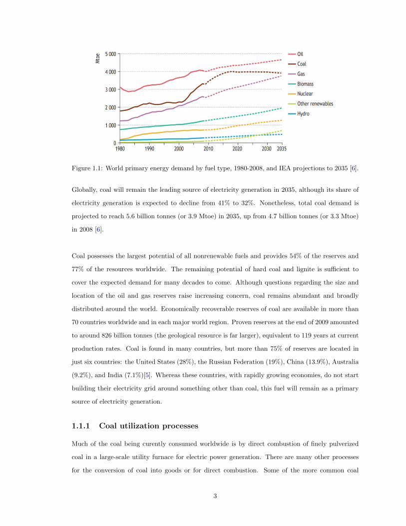
Figure 1.1: World primary energy demand by fuel type, 1980-2008, and IEA projections to 2035 [6].
Globally, coal will remain the leading source of electricity generation in 2035, although its share of
electricity generation is expected to decline from 41% to 32%. Nonetheless, total coal demand is
projected to reach 5.6 billion tonnes (or 3.9 Mtoe) in 2035, up from 4.7 billion tonnes (or 3.3 Mtoe)
in 2008 [6].
Coal possesses the largest potential of all nonrenewable fuels and provides 54% of the reserves and
77% of the resources worldwide. The remaining potential of hard coal and lignite is sufficient to
cover the expected demand for many decades to come. Although questions regarding the size and
location of the oil and gas reserves raise increasing concern, coal remains abundant and broadly
distributed around the world. Economically recoverable reserves of coal are available in more than
70 countries worldwide and in each major world region. Proven reserves at the end of 2009 amounted
to around 826 billion tonnes (the geological resource is far larger), equivalent to 119 years at current
production rates. Coal is found in many countries, but more than 75% of reserves are located in
just six countries: the United States (28%), the Russian Federation (19%), China (13.9%), Australia
(9.2%), and India (7.1%)[5]. Whereas these countries, with rapidly growing economies, do not start
building their electricity grid around something other than coal, this fuel will remain as a primary
source of electricity generation.
1.1.1 Coal utilization processes
Much of the coal being curently consumed worldwide is by direct combustion of finely pulverized
coal in a large-scale utility furnace for electric power generation. There are many other processes
for the conversion of coal into goods or for direct combustion. Some of the more common coal
3

combustion or gasification methods include fixed beds, fluidized beds and entrained flow methods.
This work focuses on the latter technology, in which a pulverized fine coal flow with air/oxygen is
burned or gasified in a reactor. The coal is crushed, dried and pulverized to a fine powder. The
particles devolatilize, ignite and burn, leaving ash; the residence time of the pulverized coal par-
ticle in the furnace is typically a few seconds, and is usually sufficient for nearly complete combustion.
The pulverized coal burners used in the entrained flow systems are of two main types: swirl burners
and jet burners: swirl burners are double concentric, with a central flow containing the coal and
primary (transporting) flow and an annular hot secondary (combusting) flow, with an expansion at
the nozzle that accommodates the jet expansion. The coal and primary fluid stream as well as the
secondary fluid stream are introduced into the furnace with a strong, swirling rotation. The burner
geometry, as well as the swirls level, determine the flow and mixing patterns, which in turn then
determine coal ignition. Swirl burners are usually mounted on the furnace walls, with the burner
axis being normal to the walls. These burners are used mostly for burning bituminous coals. On the
other hand, in the jet burner arrangements, the coal and primary stream as well as the secondary
stream are introduced into the furnace as jets from the vertical nozzle arrays with no rotation. The
burners of this type are often placed at the extreme of the furnace so that the coal and the fluid
stream jets are tangential to an imaginary vertical cylinder in the middle of the combustion cham-
ber. This creates a recirculation region that burns the incoming fresh gas-solid fuel mixture, acting
as a flame envelope. The burners are usually used for coal with high moisture content such as lignite.
The main advantages of pulverized coal combustion are high reliability, full automation, adaptation
to a wide range of coal types and operating requirements, excellent capacity for increasing unit size,
and cost-effective power generation.
1.1.2 Carbon capture, utilization and storage technologies
Carbon capture, utilization and storage (CCUS) is one of the most cost-effective solutions available
to reduce emissions from some industrial and fuel transformation processes - especially those that
inherently produce a relatively pure stream of CO2 such as natural gas and coal-to-liquids process-
ing, hydrogen production from fossil fuels and ammonia production. In some cases, CCUS can be
applied to these facilities at a low cost as USD 15-25 per tonne of CO2, and provides an opportunity
to reduce CO2 emissions by avoiding the current practice of venting CO2 to the atmosphere [6].
4

CCUS technologies are expected to play a critical role in the sustainable transformation of the indus-
try sector. Today, 16 large-scale CCUS applications at industrial facilities are capturing more than
30 million tonnes (Mt) of CO2 emissions each year from fertilizer (ammonia), steel and hydrogen
production, and from the natural gas processing [6].
Other critical issues that require intensive R&D before applying the oxy-coal technology include the
following [5]:
• Recirculation of the flue gas: involves the determination of the ”place of extraction”. This is
a function of the type of RFG, namely, cold and dry, cold and wet, or hot and wet RFG.
• Corrosion: material choice, controlled flame temperatures, and excess oxygen ratio.
• Combustion stability: flame temperature, shape and stability, oxygen concentrations, partial
loads, the volume of the RFG, and the place of the flue gas (FG) extraction.
• Startup and shutdown conditions: burner design and burner setting.
• Thermal efficiency: heat transfer inside the convective part of the furnace.
• Air separation unit (ASU) and CO2 compression: oxygen quality, FG composition, emissions,
etc.
• Slagging and fouling: ash quality, composition of the combusting gas, and flame temperature.
• Burner design: flame characteristics, oxygen concentration and its distribution among different
streams, gas velocities, number of burners, etc.
• Boiler design: retrofit or new designs.
Finally, it can be concluded that oxy-coal is a zero CO2 emission emerging technology with a
strong commercial interest. Combustion science and modeling are needed to advance the oxy-firing
technology and to optimize operations, especially when this effort is associated to pilot-plant trials
and the further design of a plant. There are already several demonstrations projects planned for
pulverized fuel (PF) oxy-fuel technology, a 30 MWth pilot plant and a 250 MW demonstration plant
in Schwarze Pumpe, Germany; a 30 MWth retrofitted boiler in Biloela, Australia, and a 30 MWth
pilot plant and a 323 MW full-scale demonstration plant in El Bierzo, Spain [5, 7]. The realization
5

of these projects will bring valuable information that is necessary to understand the effect of a CO2-
rich atmosphere on oxy-combustion of PF in real scales and important information for the potential
scale-up and construction of a CO2 emission-free, coal-fired power plant.
1.1.3 Staged, pressurized oxy-combustion
Staged, pressurized oxy-combustion (SPOC) is a CCUS technology, being developed at Washing-
ton University in St. Louis (WUSTL). Offers high overall power plant efficiency that is feasible
with first-generation atmospheric oxy-combustion. By separating the overall fuel burn into multiple
stages (Fig. 1.2), the quantity of needed recyled flue gas (RFG) can be greatly reduced as the
resultant flame temperature for each individual stage is managed easier due to the lower fuel firing
rate. The SPOC system is also pressurized, making the flue gas volume smaller than with conven-
tional atmospheric oxy-combustion, yielding a smaller overall footprint and lower downstream CO2
compression power requirements. Another benefit of operating at elevated pressures is gas-side heat
transfer enhancement, reducing the quantity of boiler bank tubing needed to achieve the thermal
absorption.
Figure 1.2: Comparison between conventional and SPOC technologies [8].
As the produced flue gas contains a large component of moisture, either directly from the fuel, or
from the hydrogen combustion, a significant amount of moisture latent heat is available. Pressurizing
allows the capturing of this energy, normally represented by the difference between the gross calorific
6

value (GCV) and the net calorific value (NCV) of the fuel. This energy is normally lost to the
environment via the stack in conventional air-fired combustion plants, or to the cooling system for
the case of atmospheric oxy-combustion systems. The partial pressure of the moisture in the SPOC
process allows the condensation of this moisture to occur at temperatures that are beneficial to the
steam cycle.
Figure 1.3: Schematic of the SPOC technology [8].
In a traditional boiler, the fuel is generally supplied with an amount of oxygen that is in slight
excess (in the range of 15%) of that required for stoichiometric (theoretical condition for which
there is enough oxidizer to completely burn all the fuel) combustion of the fuel to ensure complete
combustion. On the other hand, in the staged combustion approach, in the first stage, there is an
over-supply of oxygen, as characterized by the equivalence ratio φ (which is defined as the ratio of
the mass of oxygen supplied to the mass of oxygen required for stoichiometric combustion of the
fuel), exceeding unity, φ > 1. The large amount of O2 excess, effectively acts as a diluent, thereby
assisting in the control of the temperature of the combustion products and heat transfer. In the
SPOC process, heat is extracted from the first stage into the Rankine steam cycle. Once the flue gas
temperature is sufficiently reduced, the combustion products from stage 1, including O2 excess, are
passed to stage 2, where additional fuel is injected and more O2 is consumed. This process continues
in multiple stages until nearly entire O2 is consumed, Fig. 1.3.
7

If the fuel feed rates at each stage are equal, the number of stages required and the equivalence ratio
of the first stage are nearly similar if almost all of the oxygen in the final stage is to be consumed.
Four stages were chosen in order to maintain a global adiabatic flame temperature similar to air-
fired combustion. Furthermore, a conceptual design of the burner and the boiler using computational
fluid dynamics (CFD) simulations, have shown that high-temperature flame impingement on heat
transfer surfaces can be avoided and heat flux can be controlled to an acceptable level in four stages
[9].
To demonstrate the concepts of the SPOC boiler design and to validate the models experimentally,
a 100 kW presurized facility was designed and constructed. This facility was designed to accommo-
date a wide variety of gas inlet conditions (1 < φ < 3, O2 concentrations of 21 to 99%) to identify
the optimal operating conditions for the SPOC process. This 160 m2 facility located at WUSTL,
contains a furnace for studies of pressurized combustion or gasification of coal or other fuels, at a
pressure of up to 20 bar. The test furnace, Fig. 1.4, is approximately 20 ft long and is comprised of
multiple sections with access ports for instrumentation. This facility includes the bulk liquid storage
and the gas delivery systems for O2 and CO2 for pressurized oxy-combustion research. The reactor
is made of refractory material, with an internal diameter of 5.5 inches and is placed at the center of
the pressure vessel, as shown in Fig. 1.4. A conical-shaped quartz tube with ignition and sampling
ports was built as the top section of the reactor; this allows for visual access to the flame and optical
diagnostics.
The combustor operating pressure has a critical impact on the overall performance of the pressur-
ized oxy-fuel combustion power cycle. By increasing the operating pressure, the thermal energy
recovery from the flue gases grows as more available latent enthalpy at higher dew point is recu-
perated. The maximum efficiency can be achieved in the vicinity of the 10 bar operating pressure
[10]. Given that the high pressure system raises the flue gas density and reduces the equipment
size, the best system from an economic standpoint might be found at higher operating pressures.
Moreover, Gopan et al. [11] studied the appropriate operating pressure for the boiler, considering
an analysis of the flue gas moisture condensation, effective SO2 and NOx removal and heat transfer
to the direct contact column (DCC), revealing that increasing combustion pressure beyond 16 bar,
does not lead to a significant increase in overall efficiency. Based on these considerations, a pressure
of 15 bar was selected. Throughout this thesis, all numerical simulations were conducted at the same
pressure as the WUSTL experimental facility. Another important aspect in the SPOC technology
8

Figure 1.4: A photo (a) and schematic (b) of the WUSTL 100 kW pressurized oxy-combustionfacility [8].
is to reduce the high flame temperatures, which may cause excessive wall heat flux and slagging. To
avoid flame impingement and slagging on the walls, a high level of symmetry throughout the pres-
sure vessel needs to be maintained. Hence, to maintain axisymmetric flow, buoyancy forces restrict
the pressure vessel and burner to be oriented vertically. This is very different from the traditional
atmospheric pressure boilers, which are typically up-fired with the burners placed horizontally on
the vertical walls. For SPOC, the axisymmetric burner arrangement is preferred, with the burner
down-fired from the top of the cylindrical pressure vessel. Down-firing from the top (as opposed to
up-firing from the bottom) avoids the possibility that ash/slag build up will fall on the burner.
Xia et al. [9], used CFD simulations to show a concept design for the SPOC boiler where, even at
very low flue gas recycle, the wall heat flux for all stages was controlled to manageable levels for
utility-scale applications. However, a practical constraint is the high oxygen concentration next to
the boiler tubes, creating a risk of metal fires if an ignition source, such as an impacting ash particle,
is present. Therefore, to provide a safe operating condition, the oxygen concentration next to the
wall should not exceed a maximum admissible level. To avoid negative impacts of the flame shape
and wall heat flux, the initial section of the boilers is designed as the frustrum of a cone, as shown
in Fig. 1.5, which helps to maintain a low Richardson number, Ri = gβ (Thot − Tref)L/V 2 (natural
convection relative to forced convection), where g is the gravitational acceleration, β is the thermal
9

expansion coefficient, Thot is the hot wall temperature, Tref is the reference temperature, L is a char-
acteristic length, and V is a characteristic velocity. The effectiveness of such a cone-shaped boiler
in avoiding buoyancy-induced recirculation has been demonstrated by Xia et al. [9] and Gopan et
al. [11].
Figure 1.5: WUSTL burner and initial section of the boiler designs utilized in the SPOC facility.
The Richardson number is low at the burner head because the small cross-sectional area of the
conical design yields a high stream velocity. As the flow moves downstream, the cross-sectional area
increases and the volumetric flow rate of the gas grows; as the coal devolatilizes and combusts, both
the molar fractions and the gas temperature increase. The cone angle of the boiler is designed by
matching the increasing volumetric flow rate of the gas with the increasing cross-sectional area. To
provide a safe operating condition, with the oxygen concentration next to the wall constrained to a
pre-defined maximum, while maintaining low RFG, the burner design shown in Fig. 1.5 incorporates
a central pure oxygen stream surrounded by the fuel in an annulus, which is further surrounded by
a secondary oxidizer with an oxygen concentration that can be varied. The burner operates in a
non-premixed combustion mode and incorporates three reactant streams (the fuel stream and two
separate oxidizer streams) to provide enhanced operating flexibility. A bluff body is included on the
nozzle end on both surrounding and central oxidizers of the fuel annulus to assist with flame holding.
These rings trip both oxidizer flows at the burner exit and cause small localized recirculation regions
at the burner end, which enhances flame stability resulting in predicted flame attachment for a wide
range of flows.
10

Chapter 2
Motivation and objectives
Although some, if not all, of the most important features in a practical combustion process (e.g. the
SPOC technology) are dominated by turbulence, actual CFD simulations face their most important
challenge in accurately describing this phenomenon. In the previous studies on the SPOC technology,
extensive CFD modeling of turbulence coupled with heat transfer, coal combustion, and transport
of reacting species have already been performed based on steady and unsteady Reynolds-Averaged
Navier Stokes (RANS) models [12, 13]. However, these models are not capable to appropriately
resolve the spatial-temporal turbulent scales of the flow, since some modeling in the Navier-Stokes
equations introduce artificial parameters that, if not adequately modeled in all regions of the flow,
can lead to inaccurate results. In addition, the results produced by these models are the averaged
quantities only, which may lead to missing some important turbulent structures of the flow.
On the other hand, direct numerical simulations (DNS) are used to solve instantaneous Navier-Stokes
equations, resolving all scales, down to the Kolmogorov dissipation scale without using any models.
Although these simulations can give the most accurate results, their computational requirements
are still prohibitive for real engineering flow applications. To capture the smallest structures of
turbulence, the three-dimensional grid of the investigated system should be at least N = Re9/4.
It was estimated by Jamshed [14], that for a benchmark backward-face step DNS by utilizing the
modern Cray X1 supercomputer at the Oak Ridge National Laboratory, the required calculation time
is approximately 1 day. However, the latter has more than 250 times the computational resources of
the supercomputers used in this thesis. Furthermore, the computational cost significantly increases
for simulations solving for multi-physics interaction, as occurring in the SPOC simulations.
11

As an intermediate resource between RANS and DNS, large-eddy simulations (LES) can address
some of the limitations of both models. In LES, the computational cost of DNS is reduced by intro-
ducing a so-called filter function, which purpose serves to ignore explicit solving on those turbulent
scales underlying it. The filter function is applied to the Navier-Stokes equations, and its effect
on the flow produces the resolved and sub-grid scale (SGS) fields. The latter is modeled by using
similar concepts as in RANS, such that the computational complexity is drastically reduced as the
smallest turbulent scales are not directly solved. Conversely, the resolved field is the product of
a DNS method for turbulent structures larger than the filter function, therefore not requiring any
further modeling.
This work focuses on the implementation of an LES to the ongoing SPOC experiments at WUSTL.
Figure 2.1 depicts a comparison of the flame structures obtained in the experimental facility and one
obtained in the LES modeling. The latter is worked over a structured mesh of the SPOC geometry
done in ANSYS ICEM consisting of 2.4 million cells and the CFD commericial software ANSYS
Fluent 18.1 & 19.2. The results adhere to the current experimental conditions at WUSTL’s facility
and, particularly, to the investigated coal type, flue gas recycle rates, and O2/CO2 ratios.
Figure 2.1: Illustrative comparison of the oxy-coal flames obtained in the WUSTL experimentalfacility (left) and the LES modeling (right).
12

2.1 Objectives
To assist the ongoing experiments of the lab-scale facility at WUSTL, a critical need to develop ac-
curate and reliable CFD models is needed. In the past, extensive CFD modeling of this technology
has already been performed by utilizing the k−ω SST RANS model. However, as stated previously,
some features of the turbulent flow are not observed, particularly, the instantaneous velocity fields
and formation of eddies; the structures that highly influence the motion and mixing of particles due
to turbulent dispersion.
The main objective of this thesis is to provide WUSTL with a basic understanding of an LES of the
SPOC technology, which can serve as a baseline for future investigations in this framework.
2.2 Scope of this work
In this thesis, an effort in transitioning from an already established RANS simulation towards
practical LES of the SPOC technology is performed. Particularly, two CFD studies, before and
during the transitioning between these turbulence models are explored, for this purpose:
• First, a comparison of two discrete phase models is discussed. This is performed in a converged
RANS field (before studying the LES turbulence model) employing the discrete phase model
(DPM) and the dense discrete phase model (DDPM). As suggested previously by the RANS
simulations of Udochukwu [13], in the SPOC burner, there are some zones experiencing par-
ticle clustering, causing a non-uniform particle injection into the SPOC boiler. In this study,
the effect of particle-particle interaction is added to the fluid-particle interaction and is later
compared to the results obtained without particle-particle interaction.
• Second, a detailed study on the LES SGS models is discussed, in which a successful numerical
stabilization method for a RANS-to-LES transition is derived. A thorough comparison of the
classic Smagorinsky model and dynamic-stress Smagorinsky-Lilly SGS model is performed,
discussing the drawbacks of both models and finding the most convenient discretization schemes
to be utilized for a successful RANS to LES transition.
Once with a stable LES simulation, a third study on the turbulent dispersion of particles and the
effect of particle size on potential wall impactions is presented as well. Two characterizations of
a representative fluid time scale, alongside a detailed calculation of the Stokes number of particles
13

with diameters from 200 µm up to 2000 µm are analyzed, determining the critical particle size to
be injected into the lab-scale SPOC technology.
The accuracy of the results presented here should be validated detailed grid resolution test. In this
thesis, the mesh solves for the turbulent length scales between the integral turbulent length, and
the Taylor micro-scales, calculated as l = C3/4µ k3/2/ε and λ =
√10νk/ε [15, 16], respectively, with a
characteristic mesh cell size of 1.5 mm in a central region in the flow. However, to properly capture
down to the Kolmogorov length scales, the number of the computational cells should increase at least
by an order of magnitude, i.e., 25 million computational cells (calculated using a Reynolds number
of Re≈2000 obtained in the initial conical section of the boiler using the previous RANS results [13]).
Therefore, it is acknowledged to the reader that a further effort is still necessary for terms of grid
sensitivity and integration time steps; the parameters that were used here served only for the tran-
sitioning work from the RANS to an initial LES.
This thesis has been organized as follows: Chapter 3 presents a literature review on the theory of
coal combustion, where the most important aspects relevant to these investigations are described;
Chapter 4 is devoted to a basic theory of large-eddy simulations and a brief discussion on the
SGS models utilized in this thesis; Chapter 5 overviews the CFD models utilized in the numerical
solver ANSYS Fluent; Chapter 6 presents the results of the three studies previously mentioned, and
Chapter 7 includes the conclusions and future work sections.
14

Chapter 3
Theory of coal combustion
3.1 Oxy-fuel combustion
Conventional pulverized fuel (PF) fired boilers, currently being employed in the power industry, use
air for combustion, in which the nitrogen (N2) from the air (approximately 79% vol) dilutes the
combustion products such as carbon dioxide (CO2) and H2O vapor in the flue gas. During oxy-fuel
combustion, a combination of oxygen (typically of greater than 95% purity) and recycled flue gas
is used to burn of the fuel. A gas consisting mainly of CO2 and water vapor is generated, with
a concentration of CO2 between 70% and 90%, depending on a recycle mode (wet or dry). The
recycled flue gas is used to control the flame temperature and make up the volume of the missing
N2 to ensure that there is enough gas to carry the heat through the boiler.
Oxy-fuel combustion occurring in bench- [17], pilot- [18] and demonstration-scale [19] experiments
has been found to differ from air combustion in several ways, including a reduced flame temperature,
delayed flame ignition and related flame instability, reduced NOx and SOx emissions and changed
heat transfer. Many of these effects can be explained by the differences in the gas properties between
the CO2 and N2, the main diluents in oxy-fuel gas and air, respectively. CO2 has different thermo-
physical and optical properties than N2 that influence both the reaction rates and heat transfer.
Table 3.1 shows some selected gas properties of N2 and CO2. The molar heat capacity of CO2 is
higher than that of N2, with CO2 being a bigger heat sink than nitrogen. Hence, in order to maintain
the adiabatic flame temperature at the same level as for air combustion, an increase of the O2 volume
15

fraction in the O2/RFG mixture is required. The molecular weight of CO2 is 44g/mole, as compared
to 28g/mole for N2. Therefore, the density of the flue gas is higher in oxy-fuel combustion. This
results in lower gas velocities and higher residence times of particles in the furnace.
Table 3.1: Gas properties for N2 and CO2 at 900C [20]
Property N2 CO2 Ratio CO2/N2
Thermal conductivity, 10−3, W/mK 74.67 81.69 1.09Molar heat capacity, kJ/kmol K 33.6 56.1 1.67Density, kg/m3 0.29 0.45 1.55O2 diffusion coeff., 10−4, m2/s 3.074 2.373 0.77Thermal diffusivity, 10−7, m2/s 2168 1420 0.65Molecular weight, kg/kmol 28 44 1.57Energy per volume, J/m3K 0.34 0.57 1.67
The oxygen diffusion rate in CO2 is 0.8 times higher than in N2, thus affecting the oxygen availability
at the char surface. The lower thermal diffusivity of CO2 leads to slower flame propagation. The
higher energy per volume for CO2 results in a lower temperature of the combustion gases compared
to air-firing (if O2 is kept at the same level as for air). The high partial pressure of CO2 and H2O
vapor in the RFG results in the higher flue gas emittance. Therefore, similar radiative heat transfer
will be attained for a boiler retrofitted to oxy-fuel, when the O2 content in the O2/RFG mixture,
passing through the burner, should be less than the required levels for the same adiabatic flame
temperature.
3.2 Coal particle ignition and devolatilization
Combustion of pulverized coal is a complex process governed by a number of physical and chemical
phenomena. Development of a complete description of coal combustion requires incorporation of a
coal particle reaction model [21] into the CFD simulations. A schematic diagram of a reacting coal
particle is illustrated in Fig. 3.1. This model suggests that at any time in the reaction process, the
coal particle consists of:
1. Moisture.
2. Raw coal (volatiles).
3. Char.
4. Ash (mineral matter).
16

Figure 3.1: Schematic of coal particle combustion, illustrating constituents and reaction processes[21].
The principal steps of the reaction progress are the thermal decomposition of the raw coal and
the subsequent burnout of the char and the volatile matter. The following reaction steps typically
summarize the main process of coal combustion [5]:
Coal (raw)→ Char + Volatiles + H2O, (3.1)
Volatiles + O2 → CO + H2O + SO2 + NO, (3.2)
CO +1
2O2 → CO2, (3.3)
Char + φ−1O2 →(2− 2φ−1
)CO +
(2φ−1 − 1
)CO2, (3.4)
Char + CO2 → CO + CO, (3.5)
Char + H2O→ H2 + CO. (3.6)
As it is heated, a coal particle undergoes decomposition into char and volatile material, Eq. (3.1), the
former burning slowly in the later stages of the flame, Eqs. (3.4)-(3.6), whereas the volatile material
is assumed to rapidly form carbon monoxide (CO), Eq. (3.2) and, subsequently, CO2, Eq. (3.3), as
the most simple reaction mechanism. In the case of combustion of a PF in an O2/RFG mixture, the
high partial pressure of CO2 at the surface of hot burning particles results in the higher concentra-
tions of the surface complex C(O) on the carbon surface, which triggers the reaction of CO2 with
the char carbon to form the carbon monoxide, which diffuses away from the surface through the
boundary layer, where it combines with the inward-diffusing O2 according to Eq. (3.3). Of course,
17

many elementary reactions steps are involved in the reaction (3.3), with one of the most important
being CO + OH ↔ CO2 + H. In case of oxycombustion with wet recycling, the H2O gasification
reaction, Eq. (3.6), can play a significant role in char burnout as well.
Replacing N2 with recycled flue gas (containing mainly CO2) for dilution purposes in oxy-firing
will change the gas properties in the combustion chamber. Therefore, the effect of the changed gas
properties on the homogeneous and heterogeneous reactions as well as on the heat transfer occurring
during PF oxy-combustion is discussed here with respect to the fundamental coal combustion theory.
3.2.1 Particle ignition
Investigations of the ignition mechanisms showed that the ignition of char particles typically occurs
heterogeneously, whereas coal particles may ignite heterogeneously (caused by the coke-oxidation
reaction), homogeneously (caused by volatile-matter oxidation in the gas phase), or by a combination
of both mechanisms [22–24]. Homogeneous ignition is favored by high oxygen concentrations and
close particle interactions. Ponzio et al. [23] have investigated the ignition behavior of coal particles
at different oxidizer temperatures (870 - 1273 K) and oxygen concentrations. The ignition behavior
was classified into: (1) sparking ignition by heterogeneous oxidation of the non-devolatilized coal
at high oxidizer temperatures and medium-to-high oxygen concentration, (2) flamming ignition by
homogeneous ignition of volatiles for high oxidizer temperature and low oxygen concentrations; and
(3) flowing surface ignition by heterogeneous oxidation of char at low oxidizer temperatures and
low oxygen concentrations. Furthermore, it was indicated that the influence of oxidizer temperature
and concentration was smallest at a high oxidizer temperature. Baum and Street [25] reported that
heterogeneous ignition occurs not only on the outer surfaces of particles but also inside the pores.
They concluded that the ignition and combustion of the great majority of particles of size typical for
PF firing, is chemically controlled. At high surface oxidation temperature, two ignition jumps were
observed by Gururajan et al. [26]: the first due to the heterogeneous mechanism, and the second
due to the homogeneous one. Consideration of the simultaneous occurrence of volatile combustion
and surface oxidation shows that the surface oxidation influences the ignition temperature of only
small particles or at high oxygen concentration. The model predictions by Mitchel et al. [27]
showed that relatively little CO2 is formed in the boundary layers of small particles (less than 100
µm). Correspondingly, little thermal energy is transferred to the particle surface as a result of CO
conversion in the boundary layer. Therefore, for small particles, any CO2 formation should occur
18

on the particle surface, not in the surrounding gas.
3.2.2 Coal devolatilization
Devolatilization (or pyrolysis) is the first stage of the coal combustion process and its behavior is
the most important aspect of the role of coal quality in the combustion chemistry being primarily
responsible for the partitioning between the volatile matter and char. Therefore, it determines: (1)
the particle residence time requirements; (2) the near-burner heating rates that govern ignition,
flame stability and flammability limits of the pulverized coal flames; and (3) the soot loadings that
determines near-burner radiation fluxes. The volatiles released during devolatilization can account
for up to 50% of the heating value of coal [28]. Ultimate yields have been shown to be very similar
at about 50 wt% (mass fraction) for coals through the high volatile bituminous coal and lignites,
then diminish in coals of higher rank. However, the proportions of gases and tars vary widely,
with gas dominating the yields of low-ranked coals. The mechanisms and variables that control
coal devolatilization have been studied in detail by Smoot [29]. Only a brief description of coal
devolatilization is given here, emphasizing on small coal particles, where devolatilization is usually
kinetically controlled, with no internal particle temperature gradients.
Devolatilization occurs as the raw coal is heated in an inert or oxidizing atmosphere. The devolatiliza-
tion stage consists of three distinct physical processes: (1) pyrolysis, (2) volatile transport through
the pores, and (3) the secondary reactions changing the chemical products of gas. The pyrolysis
behavior of coal is affected by the temperature, heating rate, pressure, particle size and coal types,
among other variables [29]. Higher mass release during devolatilization generally occurs at higher
temperatures. As the coal temperature increases, the bridges linking the aromatic clusters break,
resulting in the finite size fragments that are detached from the macromolecule [30]. As core pores
melt and fuse, the subsequent formation of bubbles (filled with light gases and tar vapor) results
in swelling. Depending on the heating rate, temperature, and particle size, either a particle may
swell or bubbles may rupture. In PF firing, the bubbles normally rupture due to high heating rates,
but significant changes occur in the char morphology due to bubble formation [31]. Therefore, the
particle softening affects the ignition, particle trajectory in the furnace, reactivity, and eventual
fragmentation and size distribution [29].
In case of pressurized conditions, the more volatile components of tar are held in the particles
19

for longer times, thereby decreasing viscosity at the critical time of gas evolution. With a further
increase in pressure, the compressive external environment results in a reduced swelling [32]. The
heating rate has two effects on the devolatilization behavior: (1) as the heating rate increases,
the temperature at which volatiles are released also grows, and (2) generally, as the heating rate
increases, the overall volatiles yield increases [28, 29]. The heating rate effects can be explained by
the competition between tar formation (bridge breaking), destruction (cross-linking) and evolution
(mass transfer), all of which depend differently on the temperature.
3.2.3 Effects of CO2 on particle ignition and coal devolatilizaion
The presence of high concentration of CO2 in the bulk gas could influence the process of coal pyrolysis
in two main ways [33]:
• CO2 is a product of coal pyrolysis, which may affect the volatile composition and yield.
• CO2 is a reactant in the char gasification reaction, which may cause differences in the formation
of SO2/NOx precursors.
Messenboeck et al. [34] studied flash pyrolysis of a bituminous coal under three different conditions,
including CO2 at 1 MPa and at a peak temperature of 1000 C, heating rate of 1000 C s−1, and
holding time of 0-60 s, respectively. There were no significant effects of varying the environment to
CO2 on the volatile yield until reaching the peak temperature. But afterwards, the reactive gases
caused gasification rates much larger than expected from the previous report on char gasification
[34]. Simultaneous occurrence of the thermal cracking and CO2 gasification of the nascent char has
therefore been evidenced, whereas the rates of the gasification seem to be much higher than those
reported previously. This may be explained with the findings from Liu et al. [35] that the gasification
rate of char is very different from that of a raw coal particle, suggesting an influence of pyrolysis
time and condition on the char reactivity. This effect was more remarkable for coals with high
volatile matter content. The presence of CO2 retards single coal particle ignition [36]. According to
Yamamoto et al. [37], the ignition delay in PF oxy-firing increases, mainly due to the high value of
the heat capacity of a gas mixture with higher CO2 concentration. The results obtained by Suda et
al. [38], who investigated a PF flame in a small spherical chamber, show that the flame propagation
velocity of a PF cloud in a CO2/O2 atmosphere decreases to around 1/5 to 1/3 of that in a N2/O2
environment at the same O2 concentration level. This was found to be mainly due to the larger
heat capacity of CO2. Shaddix and Molina [36] also reported that particle devolatilization proceeds
20

more rapidly with higher O2 concentrations and decreases with the use of CO2 diluent because of
the influence of these two species on the mass diffussion rates of O2 and volatiles. Therefore, an
increased oxygen concentration for PF oxy-firing, if selected correctly, can, in principle, produce the
ignition times and volatile flames similar to those obtained under PF-air combustion conditions [36].
Molina et al. [39] studied the ignition of the groups of particles of high-volatile bituminous coal
in an optical entrained flow reactor under O2 concentrations ranging from 12% to 48%, with N2
and CO2 as diluent gas. The analysis was performed at two gas temperatures, 1130 K and 1650 K,
respectively. The standoff distance from the coal flame to the burner was used as a metric of ignition
delay and the variation in time of the flame locations as an indication of the flame stability. It was
found that at 1130 K, as oxygen concentration increased, ignition delay decreased. This difference
is more evident with N2 as a bulk gas than with CO2, by significantly delaying ignition at 1130
K. In this case, it was observed that a higher oxygen concentration had a detrimental effect on the
flame stability. This may be due to the high particle temperature at which the char-CO2 gasification
reaction is competing with the char-O2 reaction. As the gasification reaction is endothermic, this
can provoke combustion instability.
3.3 Char combustion
Char, the porous solid residue after devolatilization, consists of extensive, condensed-ring aromatic
structures and usually accounts for 30 to 70 % of the original coal. It consists of carbon and ash
with small amounts of hydrogen, oxygen, nitrogen, and sulphur. The amount and composition of
the char depends on such parameters as the coal type, pyrolysis temperature, heating rate, pressure
and particle size.
The time required for combustion of a char particle can be several orders of magnitude larger than
the devolatilization time. The chemical structure of char does not control the reaction processes
to the same extent as devolatilization, but the physical structure of char, including pore system,
surface area, particle size, and inorganic content, plays a significant role. The fundamental surface
mechanisms of heterogeneous char gasification and combustion were reviewed by Laurendeau [40],
Hurt [41] and Essenhigh [42]. The reaction undergoes both diffusion and chemical steps as follows:
1. Diffusion of reactant gases (O2, CO2, H2O, H2) from the bulk gas phase through a relatively
stagnant film (boundary layer) to the solid surface of the particle and into the particle’s pore
structure.
21

2. Adsorption of reactants on the solid.
3. Surface chemical reaction.
4. Desorption or surface reaction products.
5. Diffusion of the gaseous products into the bulk gas phase.
Laurendeau [40] has postulated the existence of three different regimes in which one or more different
processes control the overall reaction rate. This ”three-zone” theory has been widely accepted and
used to interpret experimental data in the char oxidation literature.
According to this ”three-zone” theory, char combustion rate is controlled by chemical kinetics at low
temperatures (Zone I), oxygen pore diffusion at moderate temperatures (Zone II), and oxygen bulk
diffusion at high temperatures (Zone III). However, when all reactants are considered, the definition
of reaction rate becomes extremely difficult due to the fact that different reactants have different
reactivities toward carbon in the char. It is likely that high-temperature gasification with CO2 or
H2O is kinetically controlled, whereas O2 reaction with carbon is in the diffusion-controlled regime
at the same temperature. Therefore, the factors influencing the char reactivity and reaction rates
should be studied in detail before attempting any computational work.
3.3.1 Factors influencing the char reactivity and reaction rate
Coal reactivity and reaction rate are affected by various variables that involve the coal properties and
the conditions in which reactions occur. Generally, at low oxygen concentrations, the char oxidation
phase of combustion is subsequent to the devolatilization phase. However, as the oxygen concentra-
tion increases, the whole combustion process happens progressively faster, with devolatilization and
char oxidation occurying simultaneously [43]. In addition to the reactive gases concentration, other
factors influencing the reactivity and reaction rate of the coal are:
• Pore structure: when the reaction rate is affected by the gas diffusion process, the pore struc-
ture of a char particle is a key factor in determining the gasification and combustion rates.
Depending on the type of carbon, the surface area of a char particle may increase during early
stages of gasification/combustion. Reactants penetration dictates the development of pore
structure as a char particle is consumed. Hippo and Walker [44] concluded that the reaction
develops a new surface area by enlarging micropores and opening up more volume not previ-
ously accessible to reactants. With higher temperatures, faster reactions will utilize only the
22

most accessible portion of the pore structure, favouring the development of macropores and,
hence, increasing the reaction rates.
• Pressure: devolatilization and combustion/gasification reactivities decrease with increasing
pressure [45]. Monson et al. [46] stated that in an atmosphere of constant gas composition
and reactor temperature, the rise of total pressure from 0.1 up to 0.5 MPa led to modest
increases in the area reactivity, but further increases in pressure resulted in decreasing reac-
tivities. Wall et al. [32] and Wu et al. [43] stated that char particles formed at high pressure,
undergo fragmentation during devolatilization, affecting the structure and morphology of the
char particles, resulting in higher sphericity and higher porosity of the surface area. It appears
that when the processes other than the chemical reactions, the impact of the overall pressure
on the observed conversion rate may be important.
• CO2/O2 environment: according to Shaddix and Molina [47], the presence of high CO2 con-
centration in the bulk gas could influence pulverized char combustion by: (1) hindering the
diffusion of oxygen to the char surface, hence reducing the burning rate; (2) if there is asignif-
icant heat release in the outer layer of a char particle (from CO oxidation) that is transferring
back to the particle, the higher heat capacity of CO2 may reduce the peak gas temperature
and, therefore, the heat transfer back to the particle, reducing the burning rate; (3) dissociative
adsorption of CO2 on the char surface could result in a significant surface coverage, reducing
the burning rate; and (4) gasification of char by CO2 could contribute to the overall gasifica-
tion of the char surface, increasing the burning rate; however, the endothermic character of
the Boudouard (CO2 gasification) reaction would tend to decrease the char temperature and
thereby reduce the overall burning rate.
3.4 Diffusion flames
Most of the world coal production is consumed in finely pulverized form. Practical flames in pulver-
ized coal-fired boilers are typically diffusion flames, Fig. 3.2, which are characterized by injection of
separate streams of fuel and oxidizer into the reactor. The most common practical diffusion flame is
that in pilot and large-scale utilities and industrial furnaces, where pulverized coal is pneumatically
conveyed with a small percentage of carrier gas into a furnace through several ducts [29]. In order for
the coal to burn completely, the coal-carrier gas ”primary” stream and auxiliary secondary/tertiary
gas streams must mix. In this flame, the turbulent mixing of fuel (gaseous and solid) and oxidizer
23

occurring in the diffusion process has a major impact on the coal combustion. However, gas kinetics,
particle kinetics and heat transfer are also often important. This type of flame is characterized by
very complex fluid mechanics that may include recirculating and swirling flows. Interactions of tur-
bulence and the reactions further complicate this kind of flame. Therefore, according to Table 3.2,
the diffusion flame in the SPOC requires multidimensional transient modeling with appropriate de-
scription of convective/radiative heat transfer, turbulent fluid motion, coal particle devolatilization,
volatiles-oxidizer reaction, char-oxidation and gasification, particle dispersion, ash/slag formation,
soot formation, among others.
Figure 3.2: Schematic of a simple diffusion flame [21].
Major operational variables that influence the behavior of diffusion flames include [21]: (1) reac-
tor geometry, (2) wall materials and temperature, (3) coal type and particle size distribution, (4)
moisture percentage, (5) ash percentage and composition, (6) pulverized coal stream temperature,
velocity, mass flow and coal percentage, (7) auxiliary gas streams temperature, velocity, mass flow
and swirl/recirculating levels, (8) burner configuration and location (i.e. arrangement of ducts) and
(9) operating pressure, O2/RFG composition, etc. . .
24

Tab
le3.2
:C
lass
ifica
tion
of
pra
ctic
al
coal
flam
es[2
1].
Flo
wty
pe
Pro
cess
app
lica
tion
Typ
ical
flam
ety
pe/
contr
ol
Part
icle
size
Typ
ical
math
emati
cal
com
ple
xit
y
Per
fect
lyst
irre
dre
acto
rF
luid
ized
bed
Wel
lm
ixed
,kin
etic
all
yco
ntr
oll
edIn
term
edia
te500−
1000µ
mZ
ero
dim
ensi
on
al
Plu
gfl
owM
ovin
gb
eds
Ste
ady
fixed
bed
sS
hal
ere
tort
Soli
dre
act
ion
/h
eat-
tran
sfer
contr
ol
Larg
e1−
5cm
On
e-d
imen
sion
al,
stea
dy
Plu
gfl
owP
ulv
eriz
ed-c
oal
furn
ace
Entr
ain
edga
sifi
erM
ixin
gsp
ecifi
ed,
Soli
dre
act
ion
/h
eat-
tran
sfer
contr
ol
Sm
all
,10−
100µ
mO
ne-
dim
ensi
on
al
stea
dy
Plu
gfl
owC
oal
min
eex
plo
sion
sC
oal
pro
cess
exp
losi
on
sF
lam
eig
nit
ion
/sta
bil
ity
Pre
mix
edfl
am
eK
inet
ican
dd
iffusi
on
contr
ol
Sm
all
,10−
100µ
mO
ne-
dim
ensi
on
al
tran
sien
t
Rec
ircu
lati
ng
flow
Pow
erge
ner
atio
nE
ntr
ain
edga
sifi
ers
Ind
ust
rial
furn
aces
Diff
usi
on
flam
es,
com
ple
xco
ntr
ol
(mix
ing,
gas
kin
etic
s,so
lid
kin
etic
s)S
mall
,10−
100µ
mM
ult
idim
ensi
on
al,
stea
dy
or
tran
sien
t
25

Chapter 4
Basics of large-eddy simulations
The idea of large-eddy simulations (LES) arises from the observation that in a turbulent flow, the
turbulent kinetic energy (TKE) and anisotropy (directional preference of the statistical features) are
contained predominately in the larger scales of motion, whilst the smaller scales are only responsible
for the fine wiggles of velocity fluctuations. Therefore, it is possible to characterize the flow mainly
with larger scales, while the motion at smaller scales is ”anticipated” by some means. A loose
phenomenological definition between small and large scales is provided, according to which, eddies
of scale larger than some critical length scale l are said to be large, and those below that are said to
be small. Henceforth, the two loose terms will be used without an explicit explanation.
4.1 Filtering
As mentioned above, in LES, the scales are split into a resolved part, which is obtained via a spatial
filtering operation, and an unresolved part, called the subgrid scale, [48] ı.e.,
φ (x, t) = φ (x, t) + φ′ (x, t) , (4.1)
where the overbar indicates a filtered (resolved) quantity and prime denotes a subgrid (unresolved)
scale.
A spatial filtering that operates on a space-time variable (or function) φ (x, t) to yield a filtered
quantity φ (x, t) [49] is defined by
φ (x, t) =
∫R3
G (ξ)φ (x− ξ, t) dξ, (4.2)
26

where R3 represent a three-dimensional space, dξ is shorthand for dξ1dξ2dξ3 and G is called filter
function, filter kernel or filter. Mathematically, Eq. (4.2) is known as a convolution integral; hence,
it can be written as
φ (x, t) = (G ? φ) =
∫R3
G (x− ξ)φ (ξ, t) dξ (4.3)
= (φ ? G) =
∫R3
φ (x− ξ, t)G (ξ) dξ,
where ? is the standard notation for a convolution operation of two functions. The convolution given
by Eq. (4.3) can be viewed twofold in terms of φ: the G?φ implies moving weighted averages of φ with
respect to the weight function G (x− ξ) that moves along x; φ?G can be interpreted as a continuous
superposition of translates of φ by distances ξ multiplied by a corresponding coefficient G (ξ). The
word ”filtering” used in LES will be elucidated below. By definition, linearity is automatically
satisfied, ı.e., for variables φ, ψ and constant c, one has
φ+ cψ = φ+ cψ. (4.4)
Note that the filter function given in Eqs. (4.2) and (4.3) is a function of ξ only, and independent of
x. Such a filter is known as the homogeneous or uniform filter. The filtering operation that uses a
homogeneous filter commutes with the partial derivative with respect to both space and time, ı.e.,
∂φ
∂xi=
∂φ
∂xi, (4.5)
∂φ
∂t=∂φ
∂t,
since
∂φ
∂xi(x, t) =
∂
∂xi
∫R3
G (ξ)φ (x− ξ, t) dξ =
∫R3
∂
∂xiG (ξ)φ (x− ξ, t) dξ (4.6)
=
∫R3
G (ξ)∂φ
∂xi(x− ξ, t) dξ =
∂φ
∂xi(x, t) ,
and similar rule will hold for the time derivative, provided that ∂ (G ? φ) /∂xi exists and is continuous
(Leibniz’s rule). In LES, a filter function should be selected such that the normalization property
is satisfied: ∫R3
G (ξ) dξ = 1. (4.7)
27

The purpose of this constrain is to ensure a rapid decay of the filter function at infinity in the
physical space. If a filter function is independent of the orientation of the reference frame in the
physical space, ı.e., G (ξ) depends only on |ξ| = 1, it is called an isotropic filter.
It should also be mentioned that in the case of a compressible flow, as in the simulation presented
in this thesis, the Favre-filtering is commonly used, which introduces a density-weighted filtering
operation. A Favre-filtered quantity is defined as
φ (x, t) =
∫R3 ρ (x, t)G (ξ)φ (x− ξ, t) dξ∫
R3 G (ξ) ρ (x− ξ, t) dξ. (4.8)
There is an important distinction between the filtering in LES and the Reynolds averaging. Recall
the properties associated with a Reynolds averaging. In particular, the following is true in RANS:
φ = φ, φ′ = 0, φψ = φψ. (4.9)
Yet, despite the same notation being used, the above relation does not hold for the case of filtering
operation in general, ı.e.,
φ = G ? G ? φ 6= φ = G ? φ, (4.10)
φ′ = G ? (1−G) ? φ 6= 0, φψ 6= φψ.
4.2 Favre-filtered balance equations
When filtering operation is applied to the balance equations and expressed on Cartesian coordinates
with an homogeneous filter, using the filter commutation property, as addressed in the preceding
section, one obtains the following balance equations [50],
• Mass
∂ρ
∂t+
∂
∂xi(ρui) = 0, (4.11)
• Momentum
∂ρui∂t
+∂
∂xi(ρuiuj) +
∂p
∂xj=
∂
∂xi[τ ij − ρ (uiuj − uiui)] , (4.12)
28

• Chemical species
∂(ρYk
)∂t
+∂
∂xi
(ρuiYk
)=
∂
∂xi
[Vk,iYk − ρ
(uiYk − uiYk
)]+ ωk k = 1, . . . , N, (4.13)
• Enthalpy
∂ρhs∂t
+∂
∂xi
(ρuihs
)=Dp
Dt+
∂
∂xi
[λ∂T
∂xi− ρ
(uihs − uihs
)]
+ τij∂ui∂xj− ∂
∂xi
ρ N∑k=1
Vk,iYkhs,k
+ ωT , (4.14)
where
Dp
Dt=∂p
∂t+ ui
∂p
∂xi. (4.15)
In this set of equations, the following unclosed quantities must be modeled:
• Unresolved Reynolds stresses (uiuj − uiui), requiring a sub-grid scale (SGS) turbulence model.
• Unresolved species fluxes(uiYk − uiYk
)and enthalpy fluxes
(uihs − uihs
).
• Filtered laminar diffussion fluxes for species and enthalpy. As in RANS, these molecular fluxed
may be either neglected or modeled through a simple gradient assumption such as:
Vk,iYk = −ρDk∂Yk∂xi
and λ∂T
∂xi= λ
∂T
∂xi. (4.16)
• Filtered chemical reaction rate ωk.
• The pressure velocity term ui (∂p/∂xi) is usually approximated by ui (∂p/∂xi).
These filtered balance equations, coupled to adequate SGS models [50] may be numerically solved to
determine instantaneous filtered fields. Compared to the Reynolds averaging, large eddy simulations
provide instantaneous resolved fields.
Finding models for the unknown terms in the LES balance equations (4.11) - (4.14) may follow
concepts developed in the RANS approaches, for example, by using global quantities such as the
subgrid scale turbulent kinetic energy and its dissipation rate. Nevertheless, in LES, an additional
information is available because the large-scale turbulent motions are numerically resolved. The
29

closure models may be based on the similarity assumptions, using the known largest turbulent
structures to estimate their effects of the smaller ones.
4.2.1 Sub-grid scale modeling: Smagorintsky-Lilly model
This section is not intented to give a comprehensive review of the Smagorinsky-Lilly SGS model
(such work has already been done, e.g. by Sagaut [48]). Here I rather detail the main idea and
characteristics of the SGS models used in this thesis, and try to provide a fundamental understanding
of this model. The popularity of this model is because of its simple formulation, which recalls the
Boussinesq eddy viscosity concept [48], expressing the deviatoric residual stress in terms of the
filtered (or resolved) strain rate tensor Sij . Defining the stress tensor as Tij = (uiuj − uiuj), the
Smagorinsky-Lilly closure model of the Favre-Filtered Navier Stokes equations take the form:
Tij −δij3Tkk = −νt
(∂ui∂xj
+∂uj∂xi− 2
3δij∂uk∂xk
)= −2νt
(Sij −
δij3Skk
), (4.17)
where νt is an artificial parameter called the eddy (turbulent) viscosity. Analogous to the mixing
length model, νt is constructed from
νt = C2s∆4/3l
2/3t |Sij | = C2
s∆4/3l2/3t
(2SijSij
)1/2, (4.18)
where lt is the turbulence integral length scale and Cs is called the Smagorinsky constant, whose value
is typically between 0.10 and 0.20 for most general incompressible flow applications [51]. Equation
(4.18) can be further simplified, assuming that the integral scale lt is of the order of the grid size
lt ≈ ∆, to
νt = (Cs∆)2 |Sij | = (Cs∆)
2(
2SijSij
)1/2, (4.19)
with
Sij =1
2
(∂ui∂xj
+∂uj∂xi
). (4.20)
Unfortunately, one major drawback of this model is its inability to represent correctly all the fea-
tures of the turbulent flow with a single constant Cs, being too dissipative, especially in the near-wall
regions. From Eq. (4.19), one sees that the SGS production of the turbulent eddy viscosity offered
by the Smagorinsky model is always positive, hence there is no backscatter in this model and the
kinetic energy is transferred everywhere from the filtered motion to the residual motion. The op-
timal value of Cs depends on the type of the flow, the Reynolds number, and the discretization
30

scheme. Alternatively, the Germano dynamic SGS model or the Dynamic Stress Smagorinsky-Lilly
SGS model [52] estimates the small scale dissipation from the knowledge of the resolved eddies; see
Fig. 4.1. The Smagorinsky approach is improved through an automatic determination of the model
constant Cs = Cs (x, t) depending on time and space.
Figure 4.1: Graphical representation of the Germano identity, Eq. (4.23), in the energy spectrum.The unkown unresolved Reynolds stresses at the filter level, Tij and at the test filter level Tij arerelated through Lij , which is the LES-resolved part of the unresolved Reynolds stresses Tij [50].
The basic idea is to make use of the known filtered field u (x, t). By performing a second filtering
operation on this known field, one may extract information useful for determining Cs. For this
purpose, two filters of the same type with different filter widths are introduced, namely, a grid filter
and a test filter. The grid filter has a filter width ∆, which typically is proportional to the cubic
root of the cell volume, e.g., ∆ = V 1/3; the test filter has a filter width ∆, which is larger than ∆
and typically taken to be twice of ∆. The unresolved subgrid momentum fluxes are:
Tij = uiuj − uiuj . (4.21)
The unresolved fluxes at the test level are:
Tij = uiuj − ui uj . (4.22)
31

The two previous relations are combined to give the Germano identity [50]:
uiuj − ui uj︸ ︷︷ ︸Lij
= Tij − Tij . (4.23)
where the left hand size term, Lij , is determined by filtering the resolved LES velociy field u (x, t)
at the test level ∆. Physically, it can be interpreted as a resolved turbulent stress [52] contributed
by the intermediate scales between the grid filter width and the test filter width. Estimating the
Reynolds stresses Tij and Tij at both the grid level and test level from the Smagorinsky model leads
to:
Tij −δij3Tkk = −2C∆
2|Sij |Sij = −2Cαij , (4.24)
Tij −δij3Tkk = −2C∆2|Sij |Sij = −2Cβij , (4.25)
where C is the parameter to determine, and αij and βij are introduced to simplify notations. Then,
the Germano identity is rewritten as:
Lij −δij3Lkk = 2C (αij − βij) , (4.26)
providing six independent equations for the one unknown model constant C such that Eq. (4.26) is
overdetermined. According to Ref. [53] to propose a minimum least-square error method is proposed,
leading to an equation for C:
C =LijMij
MijMij, (4.27)
where
Mij = 2
(∆
2 |Sij |Sij + ∆2| Sij | Sij) . (4.28)
Therefore, Eqs. (4.23), (4.24), (4.28) and (4.27) provide a complete description of this model, in
which the model constant C is obtained in a self-contained manner with no empirical specification.
This model seems to be very efficient in a large number of applications, including compressible
turbulent flows [54], and it is the preferred SGS model for the simulation presented in this thesis.
32

Chapter 5
CFD modeling of pulverized coal
combustion
In this chapter, a generalized model of the coal combustion processes, including devolatilization, char
oxidation, gas-phase oxidation, and gas-particle interaction, is presented. The physical properties of
coal and gas are also summarized. The resulting generalized model, which describes the response of a
coal particle to its thermal, chemical, and radiative environment, is required to analyze propagating
coal flames and performance of combustors.
5.1 Coal particle modeling
In pulverized coal flame calculations, additional complexity is introduced by the two-phase character
of the flow. To handle such a large variety of phenomena, two numerical approaches for particle-laden
turbulent flows are available in CFD commercial softwares: Eulerian-Lagrangian (EL) and Eulerian-
Eulerian (EE) approaches [55]. In the framework of Eulerian formalism, the particles are assumed to
behave as a fluid, and the so-called two fluid models were developed. This method allows modeling
of particle-particle stresses in dense particle flows using spatial gradients of particle volume fractions.
However, the continuum assumption used in the Eulerian particle models is not justified, because
particles do not equilibrate with either local fluid or each other as they move through the flow field.
Therefore, there is no physical justification to model particle dispersion by utilizing an analogy to
Fick’s law (effective particle diffusivity) [56]. Moreover, when combustion occurs, the reaction rate
depends on the history of each particle. Current Eulerian models are unable to account for particle
33

history, because in the framework of the Eulerian approach the transport of the individual particles
is not tracked. In addition, modeling a distribution of types an sizes of particles complicates the
continuum formulation because separate continuity and momentum equations must be solved for
each size and type.
5.1.1 Particle Lagrangian motion
Using a continuum model for the fluid phase and a Lagrangian model for the particle phase allows
a computationally inexpensive solution for flows with a wide range of particle types, sizes, shapes,
and velocities. The Lagrangian reference framework is the natural frame for treating combusting
particles. The particles are treated as discrete objects and their motion is tracked as they move
through the flow filed. It is possible to account for the non-continuum behavior of particles and
particle history effects. The easiest way to compute a particle trajectory is to solve the equation
of position and motion in a fluid. In such approach, the Lagrangian particle equation for the mass
center position x(k)p,i of each k- particle can be written as
dx(k)p,i
dt= u
(k)p,i , (5.1)
For most practical dilute flow applications such as PF combustion, the momentum equation for a
spherical particle moving in a viscous fluid and therefore experiencing a lift force due to the local
gradients of translational velocities can be significantly simplified by neglecting the Basset, virtual
mass, Magnus, Saffmann, and buoyancy forces. Therefore, it can be written as:
du(k)p,i
dt=
1
τp
(uf,i − u(k)p,i
)+gi (ρp − ρ)
ρp, (5.2)
where i represents the directions and τp is the particle relaxation time, defined as the rate of response
of particle acceleration to the relative velocity between the particle and the bulk, expressed as [16]:
τp =ρpd
2p
18µf· 24
CDRep, (5.3)
where ρp, dp, and Rep = ρfdp(uf,i − ukp,i
)/µf are the particle density, diameter, and Reynolds
number, respectively; ρf is the fluid density, µf is the fluid viscosity, and CD is the drag coefficient,
defined as:
CD = α+α2
Rep+
α3
Rep2 . (5.4)
34

Typical correlations for the drag coefficient include: the Schiller-Nauman [57], Putnam [58] and Morsi
& Alexander [59] models. The latter is utilized in the current work, since it is a widely accepted
drag model for the multi-phase flow simulations, which calculates, accurately, the drag coefficient
for various particle Reynolds number. The main problem of solving Eq. (5.2) is to estimate the
instantaneous fluid velocity at each particle location uf,i as the particle moves in discrete time steps
through the Eulerian fluid velocity (the Navier-Stokes) field. In this thesis, a user-defined function
(UDF) was utilized to calculate the interpolated fluid velocity at the current particle position by
looking at the cell centroid-based LES resolved velocity fields.
5.1.2 Fluid-particle interaction: coupling mechanism
To determine the influence of the fluid flow on the particles and viceversa, Elghobashi [60] proposed
a classification map of particle-laden turbulent flows for various flow regimes, see Fig. 5.1. This
suggests the coupling method that should be utilized for an accurate modeling of a two-phase flow.
The quantities appearing on the dimensionless coordinates are the Stokes number, St (defined as the
ratio of the particle response time τp to the characteristic fluid time scale tf ), and volume fraction
Φ (defined as the ratio of the discrete phase volume to the gas volume).
Figure 5.1: Classification map of particle laden flows [60].
According to Elghobashi [60], for the very small values of Φ (≤ 10−6), the particles have negligible
35

effect on turbulence, and the particles-turbulence interaction is termed as one-way coupling. This
means that the particle dispersion depends on the turbulent length scale but, due to a negligible
concentration of the particles in this regime, the momentum exchange between the particles and the
turbulence has an insignificant effect on the flow. In the second regime (10−6 ≤ Φ ≤ 10−3), the mo-
mentum exchange between the particles and the turbulence is large enough to alter the turbulence
structure. This interaction is usually referred as two-way coupling.
Now, in this regime and for a given value of Φ, there are two zones (A and B), depending on the
Stokes number, where the transition from A to B occurs at approximately 101. In zone A, effects of
particles on turbulence vary significantly for the Stokes number in the range 0.1 ≤ St ≤ 10. In zone
B, particularly, as τp increases (e.g. by increasing the particle diameter) for the same Φ, significant
vortex shedding takes place resulting in an enhanced production of the turbulent energy. In the
third regime, because of the increased particle loading, Φ > 10−3, flows are referred to as dense
suspension. Here, in addition to the two-way coupling between the particles and turbulence, the
particle/particle collisions takes place, hence the term four-way coupling is adopted. In the extreme
case, when Φ approaches unity, one simply has granular flow in which there is no fluid.
In the present simulation, an estimate of the volume fraction, Φ, was calculated by using the mean
diameter of the Rosin-Rammler particle size distribution (RR-PSD) and an average of 15-20 million
particles in the computational domain. The estimated volume fraction is Φ = 10−4, and if the parti-
cle Stokes numbers are in the vicinity of 100 and below (desirable for adequate turbulent dispersion
of particles), the gas-particle interaction should be modeled with a two-way coupling approach. This
means that Eq. (4.12) should be updated with the appropriate DPM source terms to account for
the influence of the particle on the fluid flow, and vice versa.
5.1.3 Particle size distribution
The RR-PSD yields the following expression for the mass fraction Yd of particles having diameter
greater than dp:
Yd = e−(dp/dp)ns
, (5.5)
where dp is the mean diameter and ns is the spread parameter (spread of the distribution). Based on
36

WUSTL analysis of the coal particle size, the parameters are applicable to the simulations presented
in this thesis are summarized in Table 5.1:
Figure 5.2: Comparison of the theoretical and numerical probability density function (PDF) of theRosin-Rammler particle size distribution (RR-PSD) in a non-reacting LES field.
Table 5.1: Input parameters for the RR-PSD in the LES simulation
Min. dp Mean. dp Max dp ns
5 µm 65 µm 200 µm 3.5
However, after a manual inspection of a particle sampling for sufficient residence time for the particles
in a preliminary non-reacting LES field, ANSYS Fluent reported a deviation of the spread parameter
from ns = 3.5 (defined) to ns = 2.84 (sampled) on the theoretical probability density (PDF) function
of the RR-PSD (derivative of Eq. (5.5)).
fd = Yd
(ns
dp
)(dp
dp
)ns−1
. (5.6)
This deviation is represented in Fig. 5.2, where ANSYS Fluent produces a slightly more left-skewed
mass distribution function. This may be caused by to the numerical treatment of the bin size as
implied by the discrete set of different particle diameters within the prescribed range. Such an ad-
justment is not critical for the current simulation since small particles are studied here. However, for
the future CFD simulations, the spread parameter should be carefully incorporated to the RR-PSD,
especially when including wider particle diameter sets.
37

5.1.4 Coal combustion steps
A typical combusting coal particle is treated in ANSYS Fluent as a composition of four elements:
(1) moisture, (2) volatile matter, consisting of gases driven off during pyrolysis, (3) fixed carbon (the
nonvolatile fraction of coal), and (4) ash, the inorganic residue remaining after combustion. Figure
5.3 shows an schematic of WUSTL four elements in a coal particle and its corresponding reactions
during combustion.
Figure 5.3: Schematic of a typical coal composition based on a proximate analysis.
Table 5.2: Coal composition of the PRB sample.
Proximate analysis (w/%) Ultimate analysis (w/%)
Fixed Carbon 0.4008 C 0.7466Volatile 0.4406 H 0.0545Moisture 0.075 O 0.1824Ash 0.0836 N 0.0165
The mass fractions of these elements are provided by the proximate analysis of the coal. Similarly,
the ultimate analysis determines the mass fractions of atomic C, H, O, N of the investigated type
of coal. Table 5.2 details the composition of a Powder River Basin (PRB) coal sample, which is the
coal used in the experimental facility.
As the particles travel throughout the SPOC setup, they react according to the mechanisms detailed
in Sec. 3, which is discussed again here, in terms of the numerical modeling:
1. Drying: when a small pulverized coal particle is inserted into the burner, upon entry into
the gas stream, heat is convected and radiated to the particle surface and conducted to the
38

Figure 5.4: Thermal evolution along combustion steps for a pulverized coal particle.
particle. Typically, for small particles, water is vaporized and rapidly forced out through the
pores of the particle before volatiles are released. For the particles to be considered ”small” in
a sense that the temperature gradients within the particle are small, the Biot number:
Bi =hdpkp
, (5.7)
where h is the heat transfer coefficient to the particle, dp is the particle diameter, and kp is
the thermal conductivity of the particle, should be Bi<0.2 [61]. The rate of heat transfer to
the particle depends on the gas temperature. In this work, the particle radiation is included
via UDF-modified particle emissivity. The particle temperature is updated according to a
heat balance that relates the sensible heat change in the particle to the convective and latent
heat transfer between the pulverized coal and the continuous phase. For the evaluation of the
convective heat transfer coefficient, the particle film temperature:
Tm =Tp + Tg
2, (5.8)
is used alongside with a Nusselt number correlation. Ranz and Marshall [62] found that for
small particles with low vaporization rates, the Nusselt number Nu, obeys these equations:
Nu =hdpkg
= 2 + 0.6Re1/2p Pr1/3, (5.9)
where kg is the thermal conductivity of the gas phase.
2. Devolatilization: as discussed in Sec. 3.2.2, coal devolatilization is one of the most important
39
processes in pulverized coal flames, and it strongly influences the ignition, flame stability, heat
transfer and char burnout. The process itself represents the breakdown of the initial coal par-
ticle into a mixture of lighter gases and tars. In order to model the coal pyrolysis in a flame,
the chemical percolation devolatilization (CPD) model proposed by Fletcher et al. [63] is uti-
lized in the SPOC simulation. This model is capable of predicting the devolatilization process,
volatile species production, and the coal structure under various devolatilization conditions
(pressure, temperature, heating rates) and for a wide range of coal types.
3. Char combustion: is the final step of pulverized coal combustion. Since the interior of the
particle is dry and pyrolyzed, oxygen can diffuse through the external boundary layer and
into the char particles. The char surface reaction generates primarily CO, which then reacts
outside the particle to form CO2. The surface reactions may raise the temperature of the char
above external gas temperature when oxygen is present.
A simplified multiple-surface reaction model is used to estimate the contribution of gasification
reaction to char consumption on oxy-fuel combustion. The reactions are assumed to be 1st or-
der (forward) following the Smith approach [64], but three global char oxidation and gasification
reactions are considered:
Char +1
2O2 → CO, (5.10)
Char + H2O→ CO + H2, (5.11)
Char + CO2 → 2CO. (5.12)
The char reaction rate for reaction i, mc,i depends on the rate of reactant transport by external
diffusion and the surface reaction kinetics:
mc,i = πd2pPi,gkdiff,ikkin,ikdiff,i + kkin,i
, (5.13)
where the kinetic rate constants of the char surface reactions obeys Arrhenius law:
kkin,i = AiTβp e
−EiRuTp . (5.14)
Diffusion controls the char-oxygen reaction rate at high temperatures. Following the approach de-
scribed by Smith [64], the corresponding mass transfer limited reaction rate constant kdiff,i, can be
40
expressed as:
kdiff,i = Ci ·T
3/4m
dp, (5.15)
where Ci is the overall mass diffusion-limited constant,
Ci = νiMWc
MWi· MW
RuT7/80
· Sh ·Di,0
(ρ0P
), (5.16)
νi is the stoichiometric coefficient of carbon, MW is the average molecular weight of the gas mix-
ture in the boundary layer, and various Di,0 are the modified diffusion rates for pressurized oxy-
combustion.
5.2 Gas-phase modeling
As discussed before, the adequate model for simulating gas phase coupled to the motion of discrete
particles is the Eulerian-Lagrangian approach. Here, the two-phase flow model includes mass, mo-
mentum, energy and species balance equations into the solution of both gas and particle phases. An
LES simulation based on the SGS model described in Sec. 4.2.1 was utilized to describe the turbu-
lent flow fluctuations. Particularly, as compared to RANS, the LES model enhances the accuracy of
the reaction rates and turbulent dispersion of particles by resolving more accurately the turbulent
scales and the mixing rates.
5.2.1 Radiation heat transfer
Radiation heat transfer (RTE) is modeled by solving the RTE equation at position ~r in the direction
~s, which is given by [65]
dIλ (~r,~s)
ds+ (κλ + σs,λ) Iλ (~r,~s) = κλn
2Ib,λ +σs,λ4π
∫ 4π
0
Iλ
(~r,~s
′)
Φ(~s,~s
′)dΩ′, (5.17)
where s is the path length, κ is the absorption coefficient, αs is the scattering coefficient, n is the
refractive index, and I is the radiation intensity which depends on the position ~r and direction of
~s. The simulations in this thesis consider the gas mixture to be an absorbing and emitting medium
without scattering. After integrating Eq. (5.17) over the whole radiation spectrum, it reads
dI (~r,~s)
ds= αn2
σT 4
π− αincidentI (~r,~s) , (5.18)
41

where α is the Planck-mean absorption coefficient, and αincident is the mean incident absorption co-
efficient, both averaged over the whole spectrum weighted by radiation intensity. These properties
are functions of gas composition, temperature and pressure. Since prediction of these parameters are
computationally complex, models for absorption properties, such as the gray gas or band models,
are required to describe the radiation heat transfer.
The most commonly used gray gas model in CFD is the weighted sum of gray gas model (WSGGM)
proposed by Smith et al. [66]. In this model, the gas is assumed to consist of a transparent gas and
several gray gases, without any wavelength dependence, and the model parameters are based on the
radiation properties of the oxy-fired flue gases.
In this work, a UDF-based WSGGM is incorporated following a Planck mean absorption coefficient
of the gas mixture over a path length, s, determined by [67]:
α = −ln (1− ε) /s, (5.19)
where s is the radiation beam length, and ε is the gas emissivity. The latter is calculated as
ε =∑i
αε,i (T )(1− e−κipis
), (5.20)
where αε,i is the emissivity weighting factor for gray gas i, κi and pi are the pressure absorption
coefficient and partial pressure of the absorbing gas, i, respectively.
The emissivity weighting factors in Eq. (5.20) are the polynomial correction that can be expressed
as a function of the gas temperature
αε,i =∑j
bε,i,jTj−1, (5.21)
and are modified to reflect the actual pressurized oxy-combustion conditions.
5.2.2 Gas-phase reactions
Gas phase reactions play an important role in combustion and gasification. Light gases, hydrocar-
bon gases (alkenes and alkyls) and tar are produced alongside CO2, H2O, and pyrolysis during coal
devolatilization [68]. The species CO and H2 produced from the char particle gasification reactions
42

are also burned in the free stream outside the coal particle boundary layer for typical pulverized
coal sizes [65]. In a CO2-rich environment, the global reaction rates might be different from conven-
tional air-fueled combustion due to the chemical effects of CO2. Therefore, the modeling of gas-phase
reactions should be modified as well. This includes both the reaction mechanism and the turbulence-
chemistry interaction model.
Toporov et al. [69] proposed a simplified two-step reaction mechanism for volatile combustion in the
CFD simulation of oxy-coal combustion, which consists of volatile decomposition and irreversible
combustion of CO and H2, see Eqs. (5.22)-(5.24). Transport equations for the mass fractions of eight
different gas species (volatiles, oxygen, water-vapor, carbon monoxide, nitrogen, hydrogen, methane
and bulk carbon dioxide) were calculated with source terms defined according to the reaction mech-
anism:
Volatiles + 1.07O2 → 1.16CO + 1.7H2O + 0.03N2, (5.22)
CO +1
2O2 → CO2, (5.23)
H2 +1
2O2 → H2O, (5.24)
CH4 +3
2O2 → CO + 2H2O, (5.25)
where the stoichiometric coefficients of the devolatilization reaction were based on the corresponding
composition of the coal, see Table 5.2. In addition, combustion of methane, Eq. (5.25), was consid-
ered to include a pilot-assisting methane flame in the SPOC, which splits the total thermal power
of the lab-scale combustor into 90 kW and 10 kW from coal and methane combustion, respectively.
5.2.3 Turbulence-chemistry interaction
In turbulent flames, as in the case of the SPOC technology, turbulent fluctuations become important
and chemistry-turbulence interactions must be modeled while considering the effects of turbulent
fluctuations on the source terms of the species equations, see Eq. (4.13). The description of the
turbulence-chemistry interaction, therefore, becomes an important concern in accurately modeling
the gas-phase reaction under oxy-fuel conditions.
The eddy dissipation model (EDM) [70] was used in some numerical studies of oxy-coal combus-
43

tion [71, 72] where the chemical reaction is governed by the large-eddy mixing time scale, based on
the eddy break-up model (EBU) proposed by Spalding [73]. As a further development, the finite
rate/eddy dissipation model was proposed, in which the reaction rate is taken to be the the low-
est between of the Arrhenius reaction rate and eddy dissipation rate. In the flame zone, the eddy
dissipation rate is generally smaller than the Arrhenius rate, and the reactions are limited by the
extent of mixing. Based on the assumption that the reaction rate is limited by both the mixing of
the reactants and the heating of the reactants through the mixing with the hot reaction products,
the net rate of production of species i due to reaction r,Ri,r, is given by the smaller of the reactant
mixing rate (first term) and product mixing rate (second term):
Ri,r = min
(ν′
i,rMw,iAρτ−1SGSmin
(YR
ν′R,rMw,R
), ν′
i,rMw,iABρτ−1SGSmin
( ∑P YP∑N
j ν′′j,rMw,j
)), (5.26)
where A and B are some model constants, ν′
i,r and ν′′
i,r are the stoichiometric coefficients for the
reactant i and the product j in reaction r, Mw is the molecular weight, τ−1SGS is the SGS mixing rate,
and YR and YP are the mass fractions of any reactant and product species, respectively.
5.3 CFD modeling summary
The SGS models for turbulence, reaction and radiation in conventional atmospheric air-coal combus-
tion have been modified to account for various characteristics of oxy-coal combustion. The effects of
the physical properties of the CO2-rich stream on combustion have been investigated using the CFD
approaches, offering insight into oxy-coal combustion1 However, the development and validation of
more accurate sub-models are still needed for pressurized oxy-coal combustion systems [67].
In the present work, the flow field was solved using the SGS Dynamic Stress Smagorinsky-Lilly turbu-
lence model with the semi-implicit pressure linking equations (SIMPLE) algorithm for the velocity-
pressure coupling [74]. The species transport model for eight different species for methane-assisted
oxy-coal combustion was utilized, with modified diffusion rates for a 15 bar operating pressure. The
radiative heat source was calculated as a function of the local irradiation, calculated by the discrete
ordinates radiation model. The UDFs were utilized to modify the WSGGM for the local gas mixture
absorption coefficient and particle emissivity.
Coal particle combustion was simulated based on a two-way coupling stochastic Lagrangian proce-
44

Table 5.3: Coal particle reaction model assumptions [21].
1. Particle reaction takes place by two processes:(a) Devolatilization, which is dominated by pyrolysis of raw coal and is initiatedabove a specific threshold temperature.(b) Particle surface reaction, which is controlled jointly by oxidizer diffusion andsurface reaction. Reactions include oxygen and water vapor.
2. The particles are a mixture of discrete sets of particle sizes.3. The volume occupied by the particles is small as compared to the gas volume.5. The temperature of any given particle is uniform throughout at any given time.6. A particle is assumed to be composed of ash, moisture, volatiles, and char. Ash
is inert and any volatile mineral matter is included in the volatiles.7. The composition of volatiles, which contain hydrocarbons, nitrogen and oxygen is
specified as input for the devolatilization reactions, and it is based on the materialbalance information.
8. Devolatilization produces a fuel-rich product whose gases block diffusion and heattransfer by surface transpiration.
9. Char is consumed at a rate governed by either carbon-oxidizer diffusion or by kinetics, withother elements reacted at a rate which is proportional to their percentage in the char.
10. The product of surface oxidation is carbon monoxide, which diffuses away from theparticle and reacts further in the gas phase.
11. Particles velocities are not assumed to be identical to the gas velocity. Hence they arecalculated via Lagrangian tracking.
12. The change in char-particle diameter during burnout following devolatilization is considered.13. A global reaction in the gas-phase describes the oxidative pyrolysis of hydrocarbon fractions
from the devolatilization process to produce H2 and CO. A sequence of kineticreactions expresses the further reaction of H2 and CO, together with other gas species.
14. Local heat transfer between the gas and the particles includes convection and radiationcomponents. Required properties for the gas mixture absorption coefficient and particleemissivity are modified for pressurized oxy-combustion.
15. Moisture loss is controlled by heat transfer to the particle and by vapor diffusion from thecoal surface to the bulk gas.
dure to track the particle trajectories in the flow field. The coal particles undergo decomposition into
char and volatile material, the former burning slowly in the later stages of burning, forming CO for
the pulverized coal combustion conditions, whereas the volatile material is assumed to rapidly form
CO, and subsequently, CO2. The devolatilization process is mimicked using the chemical percolation
devolatilization (CPD) model. The input parameters for the CPD model are based on the ultimate
analysis of the coal provided by WUSTL, therefore making it sensitive to the investigated coal type.
In summary, Table 5.3 describes the assumptions applied to the CFD model in this thesis.
5.4 Computational platform
An LES model for parallel computational simulations of pulverized coal combustion under pressur-
ized oxy-fuel conditions was developed using the CFD commercial software ANSYS Fluent 18.1 and
45

19.2. These are installed in the Spruce Knob and Thorny Flat supercomputing systems, and hosted
at West Virginia University and the Pittsburgh supercomputing center, respectively. To verify the
performance of these computing platforms, tests were run on a converged LES solution at full DPM
load with approximately 20 million combusting particles in the meshed SPOC geometry (burner
diameter = 2 in, boiler diameter = 5 in, total length = 2 m) consisting of 2.4 million hexaedral cells,
see Fig. 5.5. The DPM iterations were calculated using a message passing processing, such that the
particle work was performed on the local partitions of the processors.
Figure 5.5: Structured hexaedral mesh of the SPOC geometry.
Results for 20,000 iterations showed that the Thorny Flat cluster working with one node having
Intel Xeon Gold 6126 CPU @ 2.60GHz processors (40 cores) perform better than any of the Spruce
Knob cluster configurations working with one, two or three nodes of Intel 2.3 GHz Xeon E5-2650 V2
processors (16, 32 and 48 cores respectively). Even having a higher random access memory (RAM)
in the 48 cores of the Spruce Knob cluster, the gain in performance of the Thorny Flat cluster is
evident. This can be attributed to the newer architecture and efficient allocation of the processors,
and the enhanced cache structure of the latter. Figure 5.6 shows the average wall-clock time (average
real time) per iteration for both the coupled gas-particle and pure particle solutions, where the DPM
source terms were updated every 20 gas-phase iterations, and particles were injected/tracked with
the gas phase time step. For all cases, the DPM calculation time is ≈ 50% of the coupled gas-particle
iteration time, hence revealing that a half of the computational cost is due to the Lagrangian track-
ing of the coal particles.
46

Figure 5.6: Comparison of the average wall-clock time per iteration versus number of cores for thecoupled gas-particle and pure particle phase solutions, respectively.
This preliminary test demonstrates that ANSYS Fluent shows reasonable parallel performance for
the LES simulation. When available, the best configuration is to run the simulations on machines
with at least 40 cores and an enhanced thread per execution structure. With the current computa-
tional platform, a successful LES simulation can be achieved within the order of a couple of weeks.
However, further meshing effort is still required due to the coarse mesh utilized in this thesis, since
it is aimed to establish a baseline in the LES framework only.
5.5 Solution strategy
Based upon the assumptions and theory described in the preceding sections, Table 5.3, a series of
models available in the ANSYS Fluent were chosen and setup appropriately to describe the processes
occurring in the SPOC. These are summarized in Table 5.4.
Table 5.4: CFD models applied to the simulations in this work.
Operating pressure 15 barGas phase EulerianParticle phase Lagrangian (DPM and DDPM)Fluid-particle interaction Two-way coupling mechanismTurbulence model Smagorinsky (classic and dynamic SGS sub-models)Species transport model O2,CO2,H2O,CO,H2,N2,CH4
Turbulence-chemistry interaction Finite rate/eddy dissipationDevolatilization model Chemical percolation devolatilization
(Two-step reaction mechanism)Particle combustion Multiple surface reaction
(oxidation and gasification reactiosn)Gas absorption coefficient UDF weighted sum of gray gas modelTurbulent particle dispersion Discrete random walkRadiation heat transfer model Discrete ordinates
47

The 3rd-order monotonic upstream scheme for conservation laws (MUSCL) has been employed for
the momentum, species and energy equations, while the 1st- and 2nd-order upwind schemes have
been used for the density and discrete ordinates equations, respectively. A maximum number of 20
iterations were specified in order to achieve acceptable convergence at every time step due to strong
coupling of the equations. The DPM trajectories were performed with trapezoidal and implicit
schemes for the high order and low order schemes, respectively. Appropriate boundary conditions
for the case, where the SPOC is running with a thermal power of 100 kW split into 90 kW from
coal combustion and 10 kW from methane combustion, is summarized in Table 5.5.
Table 5.5: Boundary conditions for the SPOC running with 90 kW from coal and 10 kW from CH4.
Boundary zones Prescribed value
Central oxidizer mass flow rate 15.6 g/sCentral oxidizer composition O2 0.3 vol%
Bulk CO2
Fuel inlet (annular duct) mass flow rate 2.63 g/sFuel inlet (annular duct) gas composition CH4 0.1 vol%
Bulk CO2
Coal mass flow rate 3.54 g/sCoal injection velocity 0.19 m/sSecondary oxidizer mass flow rate 19.34 g/sSecondary oxidizer composition O2 0.3 vol%
Bulk CO2
Conical section of the boiler temperature 1000 KBluff body temperature 1300 KDPM boundary conditions Walls (reflect)
Inlet / outlet (escape)
Courtesy of WVU’s emeritus professor Dr. Ismail Celik, the following solution steps were applied
before resolving with an LES turbulence model:
1. Start a cold unsteady RANS simulation without particles, at a relatively large time step.
2. Inject particles with no active combustion laws, at a consistent particle injection time step
with the fluid integration step.
3. Decrease the flow and particle integration time step by one order of magnitude.
4. Run simulation with devolatilization and char combustion. Ignite the flow patching a desired
region of domain.
5. Run for enough iterations until the fluid exits the domain.
6. Convert RANS to LES model.
48

• Use the classical Smagorinsky model: run with high Smagorinsky constant Cs and grad-
ually decrease down to the default constant.
• Use the dynamic stress Smagorinsky-Lilly model.
49
Chapter 6
Results
In this section, three CFD studies towards practical LES simulation of the SPOC technology are
presented. First, a comparison of two discrete phase models is discussed. This is performed in a
converged RANS field (before studying the LES turbulence model) for conditions detailed in the
preceding section. Second, a detailed study on the LES SGS models is discussed, and a successful
numerical stabilization for a RANS to LES transition is derived. Finally, a study on the turbulent
dispersion of particles and the effect of particle size on potential wall impactions is presented as well.
6.1 Effect of discrete phase model on the particles injection
A novel burner design, described in the introduction section is the main component in driving the
particles appropriately into the boiler. The tri-axial design with pulverized coal and gas carrier, be-
ing injected into an annulus duct, needs to be studied in terms of the DPM concentration (the ratio
of discrete phase mass to the mesh cell volume) to identify possible particle clustering or inefficient
turbulent mixing. Although the reported volume fraction in Sec. 5.1.2 (Φ = 10−4) is in the two-way
coupling region, a study on the coupling mechanisms still needs to be assessed to validate that the
CFD models are adequate to describe the particle feeding in the SPOC technology. Figure 6.1 shows
an instantaneous snapshot of the DPM contour plot inside the burner region in a RANS field.
Some chaotic behavior with relatively large coherent flow structures is observed, whereby particles
are clustering in certain regions. To validate if this phenomenon was realistic, ANSYS Fluent ex-
tended its capabilities of the DPM model to the dense discrete phase model (DDPM). The latter
is not a four-way coupling mechanism, unlike, for instance, the discrete element method (DEM).
50

Figure 6.1: Instantaneous snapshot of the DPM concentration contour plots in a RANS field utilizingthe DPM model.
Instead, the DDPM model accounts for particle-particle interaction by utilizing the kinetic theory of
granular flow (KTGF) rather than solving directly for the collisions among particles. Consequently,
the DDPM approach was tested in the same RANS field.
Figure 6.2: Instantaneous snapshot of the DPM concentration contour plots in a RANS field utilizingthe DDPM model.
This time, accounting for particle-particle interaction, Fig. 6.2 shows a similar behavior inside the
burner region, where particle clustering persists. The extent of this clustering is slightly less and
shows a tendency to concentrate in the near-wall regions, just as in the DPM case. The latter can
be explained in both models due to the amount of mass injected in the outer mesh layers at the inlet
of the annular duct. In addition, compared to the DPM model, transition to turbulent chaotic flow
starts later and further downstream in DDPM.
To measure the difference between the models, a comparison of the reported DPM concentrations
in the same converged RANS field for both models is presented in Figs. 6.3 and 6.4. Reasonable
agreement between the profiles obtained for both DPM and DDPM models is observed. Therefore,
51

Figure 6.3: Radial profiles of DPM Concentration at different axial positions along an upper half-plane slice on the particle feeding annular duct of the SPOC burner.
Figure 6.4: Radial profiles of DPM Concentration at different axial positions along a lower half-planeslice on the particle feeding annular duct of the SPOC burner.
there is no significant influence of the particle-particle interaction on the injection of the pulverized
coal particles into the burner. Furthermore, the DDPM increases the computational complexity of the
simulation and adds no benefit to the actual DPM model. From these observations, it is concluded
that the DPM model is sufficient for modeling the injection of the discrete phase into the SPOC
setup. The non-homogeneous contour plots, observed earlier, might be a result of the numerical
treatment of the particle dispersion force, particularly, by the Gaussian PDF utilized by the particle
dispersion force to include a stochastic unsteady turbulence, where the flow is potentially laminar.
However, this is a topic that requires further investigation and experimental data to validate the
conditions imposed in the injection of particles, such that the optimal mixing conditions can be
assessed to the lab-scale combustor.
52

6.2 Effect of the LES SGS model on the numerical stabiliza-
tion of the oxy-fuel flame
Since each investigated type of flow has its own unique characteristics, there is no universal Smagorin-
sky constant that can successfully represent the desired features of interest. Hence, a detailed inves-
tigation of the LES modeling is required. After reaching a statistically stable oxy-fuel flame, Fig. 6.5
with unsteady RANS modeling assessed by Udochukwu [13], the conversion to LES was investigated
by varying the Smagorinsky constant Cs in the classical SGS model. Here, the mean temperature
field shows a quite axisymmetric flame structure with the hottest region between x = 0.25 and
x = 0.35 m. The largest temperature gradient occurs axially at the inner core, x = 0.15 to x = 0.25
m, and the radial temperature gradients are symmetric. As appreciated, no turbulent eddies are
observed here, consequently having the unsteady flame converging to a steady-state solution.
Figure 6.5: Contour plot of the temperature field in a statistically stable unsteady RANS simulationjust prior transition to LES models.
According to the solution strategy presented in the previous chapter, a relatively high Smagorinsky
constant (i.e. Cs = 0.5) was utilized during a first attempt to perform the transition from RANS
to LES, to avoid an abrupt decrease of the turbulent eddy viscosity, νt. All other parameters were
maintained as in RANS, and no modification on the integration and particle injection time steps
were applied. Figure 6.6 depicts an early transition to the LES model, where the drawbacks of this
approach are evident. The flame shape was altered having the largest temperature gradients occur-
ring radially, with the flame dissipating at the axial center line for both cases, with the Smagorinsky
constants of Cs = 0.5 and Cs = 0.2. Additionally, random flame flashbacks appeared at the exit of
the central oxidizer duct. Utilizing a different approach to overcome this artificial effect, I tried a
gradual reduction of the Smagorinsky constant down to the typical value for the decay of isotropic
turbulence (i.e. Cs = 0.1), which produced an enhanced turbulent structure, as more eddies are
53

appreciated as compared to the previous cases. However, this simulation led to an eventual flame
extinction in the region near the bluff body and the introduction of numerical shocks causing oscil-
lations with a non-physical behavior.
Figure 6.6: Comparison of the temperature contour plots of three LES runs with different Smagorin-sky constants, Cs = 0.5, 0.2, 0.1 (from top to bottom), respectively.
Additionally, using high values of Cs reduces the resolution of the LES since the effect of the
turbulent eddy viscosity introduces high artificial dissipation. As discussed previously, the Classic
Smagorinsky model is an initial LES attempt, and its inability to correctly represent the oxy-fuel
flame with a single constant Cs should be addressed. Therefore, the Dynamic-Stress Smagorinsky-
Lilly SGS model was tested and studied as well. First, the conversion from RANS to LES was
54

performed, with no changes in any of the physical models or integration time steps. This time, no
explicit specification of the Smagorinsky constant was required. Second, the numerical stabilization
of this model was achieved by utilizing monotonic upstream schemes for the momentum, species
and energy. Continuity and radiation equations were solved with the 1st- and 2nd-order upwind
schemes, respectively.
Figure 6.7: Temperature contour plot of an LES with the Dynamic Stress Smagorinsky-Lilly SGSmodel.
Last and most importantly, the temporal discretization was critical to achieve a stable simulation
with this SGS model. After an extensive study, it was found that the temporal discretization scheme
needs to be bounded with a 2nd-order accuracy scheme and that after approximately 200-300 time
steps, the scheme needs to be brought back to a 1st-order scheme for ∼ 10% of the iterations com-
puted with the 2nd-order scheme. This method adds robustness and prevents the numerical schemes
to propagate any artificial effect downstream in the fluid region. Figure 6.7 shows a stable and re-
acting LES flow after a sufficient number of iterations since the transition from the RANS model.
This method needs to be applied for the required number of time steps and repeated as necessary.
The flame achieved with this method is more realistic and comparable to that experimentally ob-
served in the WUSTL SPOC facility. There are temperature gradients occurring randomly in the
boiler as a result of the turbulence-combustion interaction. Furthermore, the visualization of the
flame attached to the ring at the burner exit shows a better description of the vortex shedding past
a bluff body as compared to Fig. 6.5. This demonstrates the ability of LES to capture the high and
low temperatures as it can capture the turbulent flame fluctuations and predict the recirculation
flows more accurately than RANS.
Through the dynamic specification of Cs, the dynamic model makes a back scattering process pos-
sible. However, as pointed out by many researchers [75, 76], the resulting Cs field is found to be
highly variable and may contain a significant portion of negative Cs values, which makes an LES
55

unstable. To overcome this difficulty, the usual practice is to perform an additional averaging for
both the numerator and denominator of Eq. (4.27) over directions of statistically homogeneity (see
Refs. [52, 77]). Overall, this model is still preferred over the classical approach and is widely used
nowadays in the LES framework. The advantages of the Dynamic Smagorinsky-Lilly over the classic
Smagorinsky model are:
• Self-contained; no need to specify parameter Cs.
• Inexpensive; adds 10-15% to computational cost (vs. the classical Smagorinsky-Lilly model).
• Removes some of the problems associated with the constant coefficient in the classical Smagorin-
sky model, but needs an algorithm how to stabilize a simulation.
• Eliminates the need to prescribe the length scale
– No need to choose formula for the mesh cell size ∆, with anisotropic grid.
– Dynamic method actually computes νt rather than Cs.
• Predicts zero eddy viscosity in the laminar regions of a flow.
• No need for near-wall correction.
• No need to modify for extra strains.
It is concluded from this study, that the Classic Smagorinsky model is unable to run any LES simula-
tion for the SPOC technology. The results of this model are very sensitive to numerics, since artificial
dissipation due to numerical discretization is introduced and propagated irreversibly throughout the
flow field. The Dynamic Smagorinsky model is henceforth the SGS model utilized in the subsequent
simulations.
56

6.3 Effect of the particle size on the turbulent dispersion of
particles
A detailed investigation was performed to study the effect of particle size on the turbulent dispersion
and wall impaction of the discrete phase. First, the RR-PSD was decoupled into 3 sets of parti-
cle sizes, namely: 5-10 µm (small), 10-50 µm (medium), and 50-200 µm (big). Figure 6.8 shows
the particle tracking for these sets of particles colored by particle temperature. It is observed from
here, that the most dense particulate field is in the 50-200 µm set, as predicted previously by Fig. 5.2.
Figure 6.8: Tracking of particles of different diameters 5-10 µm (top), 10-50 µm (center) and 50-200µm (bottom) colored by the particle temperature.
The cold particles come out of the burner and recirculate for a short time period in front of the bluff
body. Consequently, they ignite, devolatilize and combust as observed in all three particle sets. The
particle temperature field is consistent with the temperature contours of the gas phase, as shown in
Fig. 6.7. In addition, all the particles contained in the RR-PSD show an adequate level of dispersion
due to efficient turbulent mixing in the conical section of the boiler.
Complementary to the temperature particulate field, a particle tracking of the discrete phase, col-
ored by the char mass fraction is observed in Fig. 6.9. This plot shows that efficient pulverized coal
57
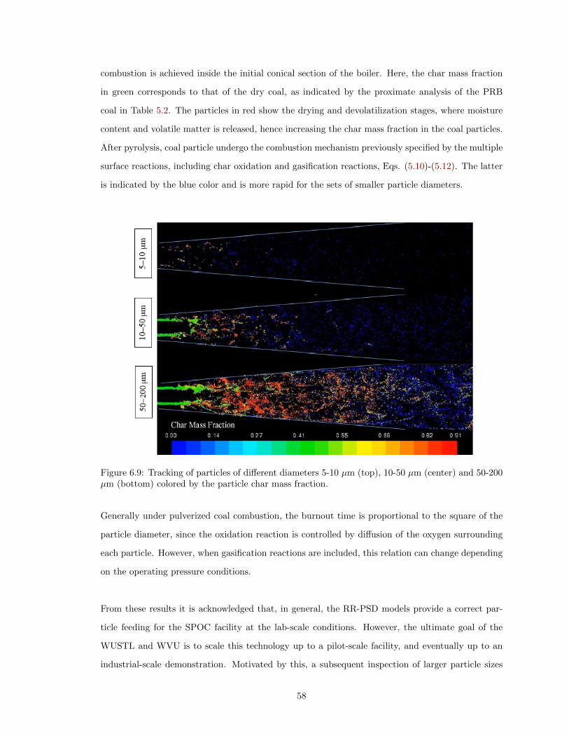
combustion is achieved inside the initial conical section of the boiler. Here, the char mass fraction
in green corresponds to that of the dry coal, as indicated by the proximate analysis of the PRB
coal in Table 5.2. The particles in red show the drying and devolatilization stages, where moisture
content and volatile matter is released, hence increasing the char mass fraction in the coal particles.
After pyrolysis, coal particle undergo the combustion mechanism previously specified by the multiple
surface reactions, including char oxidation and gasification reactions, Eqs. (5.10)-(5.12). The latter
is indicated by the blue color and is more rapid for the sets of smaller particle diameters.
Figure 6.9: Tracking of particles of different diameters 5-10 µm (top), 10-50 µm (center) and 50-200µm (bottom) colored by the particle char mass fraction.
Generally under pulverized coal combustion, the burnout time is proportional to the square of the
particle diameter, since the oxidation reaction is controlled by diffusion of the oxygen surrounding
each particle. However, when gasification reactions are included, this relation can change depending
on the operating pressure conditions.
From these results it is acknowledged that, in general, the RR-PSD models provide a correct par-
ticle feeding for the SPOC facility at the lab-scale conditions. However, the ultimate goal of the
WUSTL and WVU is to scale this technology up to a pilot-scale facility, and eventually up to an
industrial-scale demonstration. Motivated by this, a subsequent inspection of larger particle sizes
58

was studied in this LES simulation. First, particle tracers with diameters between 200 µm and 2000
µm were injected into the annular duct, simultaneously to the RR-PSD. In order to not alter the
flame shape, only 10 tracers of each size were considered. The data of the respective particle mass
and mass flow rates are detailed in Table 6.1.
Table 6.1: Mass and mass flow rates of the particle tracers.
Particle diameter, dp (µm) Particle mass, mp (mg)Particle mass flow ratemp (mg/s)
200 0.005 5.86300 0.019 19.79400 0.047 46.91500 0.09 91.62600 0.15 158.33700 0.25 251.43800 0.37 375.31900 0.53 534.381000 0.73 733.032000 5.86 5864.3
A stable LES case running for approximately 2,500 iterations, is sufficient to account for the res-
idence time of the smallest particles. The particle injection time step was ∆tp = 0.001 s, and all
particles were injected with the same velocity of the gas carrier.
As previously stated, the effect of turbulence on the particle motion is simulated in RANS by a
stochastic approach, one element of which is the random sampling of a turbulent velocity fluctua-
tion over a Gaussian PDF. However, in LES, the calculation of the instantaneous gas velocity at the
computational cell centroid uf,i makes possible to modify the particle equations of motion from a
more realistic solution.
Figure 6.10: Interpolation of the instantaneous gas velocity at the current particle position.
Therefore, a UDF was compiled to calculate the interpolated fluid velocity at the current particle
59

position. A schematic of the function of this UDF is depicted in Fig. 6.10, where the LES velocity
field computed at the cell centroid (blue dot) was interpolated to the particle position (red dot).
A second important element is the manner of determining the fluid time scale tf over which a particle
interacts with the randomly-sampled velocity field. Here, it is convenient to envision the latter as
being associated with a turbulent eddy, in which the characteristic fluid time scale is determined by
tf = le/|uf,i|, (6.1)
where the characteristic size of the randomly-sampled eddy le is the dissipation length scale [16].
Typical turbulence models that have been used to calculate the dissipation length scale include the
Prandtl mixing length and the classical k-l, k -ε models [78, 79]. The mixing length models represent
mixing or dissipation length scale of turbulence as a function of turbulent kinetic energy k and the
energy dissipation rate [79] according to the formula:
Figure 6.11: Trajectories of the 200 µm (left) and 300 µm (right) particle tracers.
60

le = C3/4µ
k3/2
ε, (6.2)
where
ε = 2νSijSij , (6.3)
and Cµ ≈ 0.09 is an experimentally proven constant. The influence of the SGS transport on the
particle motion is not considered here, which should be a reasonable assumption given the filtering
operation. Figure 6.11 shows the trajectories of the ten particle having diameters of 200 µm and
300 µm, with the averaged trajectory colored in solid blue (in the gray surfaces). As observed, the
particle dispersion is evident and there is occasional wall impaction very far downstream in the flow.
These particle sizes are more likely to follow the flow field, such that the drag force and the turbulent
eddy structures are able to alter the particle trajectories for efficient mixing.
Figure 6.12: Trajectories of the 1000 µm (left) and 2000 µm (right) particle tracers.
61

However, this is not the case for the large particles, as the trajectories for the 1000 µm and 2000 µm
tracers revealed that there is no effect of turbulence on their trajectories. Indeed, according to Fig.
6.12, the particles are injected following a straight trajectory (inside the annular duct), where due
to the burner design, they experience a change of momentum, which dominates the particle force
balance of these particle tracers as they continue throughout the SPOC. Hence, they are directed
towards the wall and no effect of turbulent dispersion is noticed.
Figure 6.13: Effect of an eddy (solid line) on the particle trajectory for various Stokes numbers [80].
The effect of an eddy on a particle trajectory for different Stokes numbers, according to Benavides
and Van Wachem [80], is graphically presented in Fig. 6.13. Therefore, the 200 µm and 300 µm
particles are in the St< 1 region since they are randomly dispersed, whereas the large particles are
in the St> 1 region, due to a dominant particle inertia. Since it is necessary to find the critical
particle size for an optimal pulverized coal feeding, it is of particular interest of this thesis to study
the case when St= 1.
As the other particle tracers in Table 6.1 were investigated, it was found that particles of 500 µm
and 600 µm experience a little effect of the turbulent eddies as observed in the St=1 case. Figure
6.14 shows these trajectories and an apparent decrease of the particle dispersion. Particles having
a diameter of 500 µm show some deviation from the mean trajectory, with few of them colliding
against the furnace wall. However, for the particles with a diameter of 600 µm, it is observed that
the dispersion with respect to the mean trajectory is vanished, hence concentrating the motion of
all particles into a single trajectory.
62

Figure 6.14: Trajectories of the 500 µm (left) and 600 µm (right) particle tracers.
To validate these observations, the particle response time for all particle diameters was calculated
according to Eqs. (5.3), (5.4) and the characteristic fluid time scale was obtained after running the
LES simulation for a considerable number of iterations while reaching statistically stable turbulence.
The latter was approximated using Eqs. (6.1)-(6.3). Therefore, the Stokes number was calculated
and plotted.
Figure 6.15 confirms that a critical particle diameter lies in between 500 µm and 600 µm, where
the transition from St< 1 to St> 1 takes place. In other words, the turbulent flow has a little to
no effect on particles larger than 500 µm. Particles exceeding this critical size most likely will be
dominated by their inertia and directed towards the furnace wall. The latter can be associated to a
geometrical design of the burner, where the duct used for injecting the particles converges axially,
hence reducing the annulus diameter. This reduction in diameter forces the particles having high
momentum to experiment an initial impaction against this convergent duct.
This result may be taken into consideration when scaling up the SPOC technology. Besides, another
definition of the Stokes number, based on the aerosol theory, by utilizing the stopping distance
63

Figure 6.15: A Stokes number map for the turbulent dispersion of particles in the lab-scale SPOCtechnology.
concept, was calculated as well. This will determine a critical particle size that may impact a wall of
the furnace. This time, the characteristic fluid time scale was computed with the arc-length between
impactions, as depicted in Fig. 6.16 and the averaged interpolated fluid velocity at the particle
positions over the corresponding arc-lengths. The arc-length s was used as the stopping distance,
and is calculated as:
s =
∫ tg
ti
|| u(k)p,i || dt. (6.4)
where ti and tf are the times of the first and second impactions, respectively.
Figure 6.16: Schematic of the SPOC showing an average trajectory for the particles larger than 500µm.
In the case of particle tracers that do not impact the wall (i.e. having a diameter smaller than 500
64

µm), the arc-length was calculated as the one having reached the same axial distance downstream
throughout the furnace for the particle tracers of the diameters exceeding 500 µm. As observed in
Fig. 6.17, a similar map is obtained when studying wall impactions.
Figure 6.17: A Stokes number map for the wall impactions of particles in the lab-scale SPOCtechnology.
This map indicates that for both phenomena, either having a poor turbulent dispersion of particles
or numerous wall impactions, the critical particle diameter for the lab-scale SPOC is between 500
µm and 600 µm. As a general recommendation, the particle feeding should not exceed a size larger
than 500 µm, such that the particles with ballistic inertia can be avoided.
65

Chapter 7
Conclusions
The main motivation for this study was to model the basic underlying mechanisms determining the
pressurized oxy-fuel combustion and, based on this knowledge, to support with a numerical study
the developing WUSTL experimental technology for reliable combustion of pulverized coal in pres-
surized oxy-firing furnaces. The LES turbulence models enhance the prediction of the oxy-coal flame
as more turbulent features of the flow are revealed as compared to typical RANS modeling. It is
noted that LES is a specialized field of research itself and, therefore, the main results obtained and
reported here, can be used only as a baseline for future LES frameworks.
In this work, two main investigations towards practical LES of the SPOC technology were conducted.
Specifically, the effect of the discrete phase modeling on the Eulerian-Lagrangian description of the
multiphase flow and the effect of the SGS model on the numerical stabilization of the LES work.
These two studies, although do not determine any critical operating condition in the experimental
facility, are important due to the need to accurately model the processes happening inside the com-
bustor. Much of the CFD work takes place in the accurate modeling of the physics and the coupling
between them. Besides, the results of this thesis intend to contribute to the still unexplored large-
eddy simulations of oxy-coal combustion. Third and lastly, an investigation of the effect of particle
size on turbulent dispersion and wall impactions was presented as well. A general recommendation
found from the latter is to feed the burner with coal particles of diameters smaller than 500 µm to
avoid a poor turbulent dispersion of particles and possible wall impactions. These problems may
cause future issues with slagging and hence, degrading the operational life of the SPOC.
66

Although the LES simulations in this thesis were able to reproduce some of the turbulent structures
of the oxy-coal flame in the SPOC, additional CFD work is still required in terms of grid sensitivity
tests. Particularly, to resolve down to the Kolmogorov scales the number of computational cells
should increase at least one order of magnitude, i.e., more than 25 million cells. However, by doing
this the reader should be aware that the computational cost might increase substantially such that
any study critical to the SPOC technology may be obtained within an order of months, instead of
weeks using the same or similar computational resources described here.
It is recalled to the reader that this thesis is a first attempt in performing an LES simulation of the
SPOC technology, in which besides to the usage of a relatively coarse mesh; a coarse flow integration
and particle injection time steps were utilized as well. It is recommended that future investigations
may be conducted first by utilizing finer temporal discretizations, and then compare them to the
results here produced. Therefore, a more detailed characterization of the turbulent time and length
scales, as well as the turbulent intensity can be assessed by increasing the sampling frequency of the
monitor points of interest.
If the above is immediately not possible, the author suggests the implementation of novel CFD ap-
proaches like detached eddy simulation (DES), which employs a hybrid combination of RANS and
LES modeling. The major benefit of DES is the possibility to split the computational domain into
zones that do not strictly require an LES model, such that RANS can perform the work without
substantially increasing the computational cost of the overall simulation (e.g. far downstream in the
boiler). However, additional care should be considered at the RANS-LES boundary zones.
Finally, any CFD work on the SPOC technology should go together with further fundamental re-
search on (1) combustion chemistry in CO2-rich environment; (2) materials and related corrosion
problems; and (3) efficient pressurized oxy-firing conditions. Furthermore, the continuous feedback
and experimental validation with the WUSTL’s lab-scale facility will bring valuable information
needed to understand the effects of a CO2-rich environment on the pressurized oxy-fuel combustion
and on the heat transfer in real industrial scales and important information for the potential scale-up
and construction of a CO2 emission free coal-fired power plant.
67

Bibliography
[1] T. F. Wall, “Combustion processes for carbon capture,” Proceedings of the combustion institute,
vol. 31, no. 1, pp. 31–47, 2007.
[2] T. Wall, Y. Liu, C. Spero, L. Elliott, S. Khare, R. Rathnam, F. Zeenathal, B. Moghtaderi,
B. Buhre, C. Sheng, et al., “An overview on oxyfuel coal combustion—state of the art re-
search and technology development,” Chemical engineering research and design, vol. 87, no. 8,
pp. 1003–1016, 2009.
[3] Y. Tan, E. Croiset, M. A. Douglas, and K. V. Thambimuthu, “Combustion characteristics of
coal in a mixture of oxygen and recycled flue gas,” Fuel, vol. 85, no. 4, pp. 507–512, 2006.
[4] M. B. Toftegaard, J. Brix, P. A. Jensen, P. Glarborg, and A. D. Jensen, “Oxy-fuel combustion
of solid fuels,” Progress in energy and combustion science, vol. 36, no. 5, pp. 581–625, 2010.
[5] D. Toporov, Combustion of pulverised coal in a mixture of oxygen and recycled flue gas. Elsevier,
2014.
[6] N. Tanaka, “World energy outlook 2010,” International Energy Agency. Paris: IEA, p. 700,
2010.
[7] T. Lockwood, “Developments in oxyfuel combustion of coal,” London, UK: IEA Clean Coal
Centre, Report No CCC/240, 2014.
[8] S. A. Hume, Z. Yang, B. M. Kumfer, R. L. Axelbaum, B. Dhungel, J. D. Slater, R. S.
Panesar, and P. J. Melling, “Improving flexibility and performance of staged pressurized oxy-
combustion,” (Melbourne, Australia), 14th International Conference on Greenhouse Gas Con-
trol Technologies, GHGT-14, October 2018.
[9] F. Xia, B. M. Kumfer, B. Dhungel, and R. L. Axelbaum, “Staged, pressurized oxy-combustion:
68

computational fluid dynamics simulations of a novel burner design,” (Clemson, SC), Eastern
States Section of the Combustion Institute, 2013.
[10] J. Hong, R. Field, M. Gazzino, and A. F. Ghoniem, “Operating pressure dependence of the
pressurized oxy-fuel combustion power cycle,” Energy, vol. 35, no. 12, pp. 5391–5399, 2010.
[11] A. Gopan, B. M. Kumfer, and R. L. Axelbaum, “Effect of operating pressure and fuel moisture
on net plant efficiency of a staged, pressurized oxy-combustion power plant,” International
Journal of Greenhouse Gas Control, vol. 39, pp. 390–396, 2015.
[12] F. Xia, Z. Yang, A. Adeosun, A. Gopan, B. M. Kumfer, and R. L. Axelbaum, “Pressurized
oxy-combustion with low flue gas recycle: Computational fluid dynamic simulations of radiant
boilers,” Fuel, vol. 181, pp. 1170–1178, 2016.
[13] G. O. Udochukwu, “Computational design of staged pressurized oxy-coal combustion,” Master’s
thesis, West Virginia University, 2019.
[14] S. Jamshed, Using HPC for Computational Fluid Dynamics: A Guide to High Performance
Computing for CFD Engineers. Academic Press, USA, 2015.
[15] H. Tennekes, J. L. Lumley, J. L. Lumley, et al., A first course in turbulence. MIT press, USA,
1972.
[16] A. Gosman and E. Loannides, “Aspects of computer simulation of liquid-fueled combustors,”
Journal of energy, vol. 7, no. 6, pp. 482–490, 1983.
[17] A. Kather and G. Scheffknecht, “The oxycoal process with cryogenic oxygen supply,” Natur-
wissenschaften, vol. 96, no. 9, pp. 993–1010, 2009.
[18] D. Toporov, M. Forster, and R. Kneer, “Combustion of pulverized fuel under oxycoal conditions
at low oxygen concentrations,” in Third international conference on clean coal technologies for
our future, May 15 2007, Sardinia Italy.
[19] F. Kluger, P. Monckert, B. Krohmer, G. Stamatelopoulos, J. Jacoby, and U. Burchhardt, “Oxy-
fuel pulverized coal steam generator development 30 mwth pilot steam generator commissioning
and testing,” 1st Oxyfuel Combustion Conference, Cottbus, 2009.
[20] H. Martin, V. Gnielinski, D. Mewes, D. Steiner, K. Stephan, K. Schaber, D. Vortmeyer, and
S. Kabelac, “Vdi warmeatlas: Berechnungsblatter fur den warmeubergang,” Verein Deutscher
Ingenieure, Springer, Berlin, 2002.
69

[21] L. D. Smoot and P. J. Smith, Coal combustion and gasification. Springer Science & Business
Media, 2013.
[22] A. Fedorov, Y. A. Gosteev, et al., “Theoretical investigation of ignition and detonation of
coal-particle gas mixtures,” Shock Waves, vol. 13, no. 6, pp. 453–463, 2004.
[23] A. Ponzio, S. Senthoorselvan, W. Yang, W. Blasiak, and O. Eriksson, “Ignition of single coal
particles in high-temperature oxidizers with various oxygen concentrations,” Fuel, vol. 87, no. 6,
pp. 974–987, 2008.
[24] D. S. Perkins, Ignition of coal and char particles: Effects of pore structure and process conditions.
PhD thesis, Rice University, 1998.
[25] M. Baum and P. Street, “Predicting the combustion behaviour of coal particles,” Combustion
science and technology, vol. 3, no. 5, pp. 231–243, 1971.
[26] V. Gururajan, T. Wall, R. Gupta, and J. Truelove, “Mechanisms for the ignition of pulverized
coal particles,” Combustion and flame, vol. 81, no. 2, pp. 119–132, 1990.
[27] R. E. Mitchell, R. J. Kee, P. Glarborg, and M. E. Coltrin, “The effect of co conversion in
the boundary layers surrounding pulverized-coal char particles,” Proceedings of the combustion
institute, vol. 23, no. 1, pp. 1169–1176, 1991.
[28] S. Saxena, “Devolatilization and combustion characteristics of coal particles,” Progress in energy
and combustion science, vol. 16, no. 1, pp. 55–94, 1990.
[29] L. D. Smoot, Fundamentals of coal combustion: for clean and efficient use. Elsevier Amsterdam,
1993.
[30] K. L. Smith, L. D. Smoot, T. H. Fletcher, and R. J. Pugmire, The structure and reaction
processes of coal. Springer Science & Business Media, New York, 2013.
[31] P. R. Solomon and T. H. Fletcher, “Impact of coal pyrolysis on combustion,” Proceedings of
the combustion institue, vol. 25, pp. 463–474, 1994.
[32] T. F. Wall, G.-s. Liu, H.-w. Wu, D. G. Roberts, K. E. Benfell, S. Gupta, J. A. Lucas, and
D. J. Harris, “The effects of pressure on coal reactions during pulverised coal combustion and
gasification,” Progress in energy and combustion science, vol. 28, no. 5, pp. 405–433, 2002.
[33] L. Duan, C. Zhao, W. Zhou, C. Qu, and X. Chen, “Investigation on coal pyrolysis in co2
atmosphere,” Energy & Fuels, vol. 23, no. 7, pp. 3826–3830, 2009.
70

[34] R. Messenbock, D. Dugwell, and R. Kandiyoti, “Co2 and steam-gasification in a high-pressure
wire-mesh reactor: the reactivity of daw mill coal and combustion reactivity of its chars,” Fuel,
vol. 78, no. 7, pp. 781–793, 1999.
[35] H. Liu, M. Kaneko, C. Luo, S. Kato, and T. Kojima, “Effect of pyrolysis time on the gasification
reactivity of char with co2 at elevated temperatures,” Fuel, vol. 83, no. 7-8, pp. 1055–1061, 2004.
[36] C. R. Shaddix and A. Molina, “Particle imaging of ignition and devolatilization of pulver-
ized coal during oxy-fuel combustion,” Proceedings of the combustion institute, vol. 32, no. 2,
pp. 2091–2098, 2009.
[37] A. Yamamoto, T. Suda, and K. Okazaki, “Mechanism of ignition delay in o2/co2 pulverized
coal combustion,” in Annual international Pittsburgh coal conference, 2004.
[38] T. Suda, K. Masuko, J. Sato, A. Yamamoto, and K. Okazaki, “Effect of carbon dioxide on
flame propagation of pulverized coal clouds in co2/o2 combustion,” Fuel, vol. 86, no. 12-13,
pp. 2008–2015, 2007.
[39] A. Molina, E. S. Hecht, and C. R. Shaddix, “Ignition of a group of coal particles in oxyfuel
combustion with co2 recirculation,” in Proc. Aiche Conf, vol. 31, pp. 1905–1912, 2009.
[40] N. M. Laurendeau, “Heterogeneous kinetics of coal char gasification and combustion,” Progress
in energy and combustion science, vol. 4, no. 4, pp. 221–270, 1978.
[41] R. H. Hurt, “Structure, properties, and reactivity of solid fuels,” Proceedings of the combustion
institute, vol. 27, no. 2, pp. 2887–2904, 1998.
[42] R. H. Essenhigh, “Rate equations for the carbon-oxygen reaction: an evaluation of the langmuir
adsorption isotherm at atmospheric pressure,” Energy & fuels, vol. 5, no. 1, pp. 41–46, 1991.
[43] H. Wu, G. Bryant, K. Benfell, and T. Wall, “An experimental study on the effect of system
pressure on char structure of an australian bituminous coal,” Energy & Fuels, vol. 14, no. 2,
pp. 282–290, 2000.
[44] E. Hippo and P. L. Walker Jr, “Reactivity of heat-treated coals in carbon dioxide at 900 c,”
Fuel, vol. 54, no. 4, pp. 245–248, 1975.
[45] J.-R. Richard, M. A. Majthoub, M. J. Aho, and P. M. Pirkonen, “Separate effects of pressure
and some other variables on char combustion under fixed bed conditions,” Fuel, vol. 73, no. 4,
pp. 485–491, 1994.
71

[46] C. R. Monson, G. J. Germane, A. U. Blackham, and L. D. Smoot, “Char oxidation at elevated
pressures,” Combustion and Flame, vol. 100, no. 4, pp. 669–683, 1995.
[47] C. R. Shaddix and A. Molina, “Effect of o2 and high co2 concentrations on pc char burning
rates during oxy-fuel combustion.,” tech. rep., Sandia National Lab.(SNL-CA), Livermore, CA
(United States), 2008.
[48] P. Sagaut, Large eddy simulation for incompressible flows: an introduction. Springer-Verlag
Berlin Heidelberg, 2006.
[49] A. Leonard, “Energy cascade in large-eddy simulations of turbulent fluid flows,” Adv. Geophys.
A, vol. 18, no. A, pp. 237–248, 1974.
[50] T. Poinsot and D. Veynante, Theoretical and numerical combustion. RT Edwards, Inc., 2005.
[51] U. Piomelli, “Large-eddy simulation: achievements and challenges,” Progress in Aerospace Sci-
ences, vol. 35, no. 4, pp. 335–362, 1999.
[52] M. Germano, U. Piomelli, P. Moin, and W. H. Cabot, “A dynamic subgrid-scale eddy viscosity
model,” Physics of Fluids A: Fluid Dynamics, vol. 3, no. 7, pp. 1760–1765, 1991.
[53] D. K. Lilly, “A proposed modification of the germano subgrid-scale closure method,” Physics
of Fluids A: Fluid Dynamics, vol. 4, no. 3, pp. 633–635, 1992.
[54] P. Moin, K. Squires, W. Cabot, and S. Lee, “A dynamic subgrid-scale model for compressible
turbulence and scalar transport,” Physics of Fluids A: Fluid Dynamics, vol. 3, no. 11, pp. 2746–
2757, 1991.
[55] ANSYS, Inc, “Ansys fluent theory guide,” Canonsburg, PA November, 2013.
[56] A. Kaufmann, Towards eulerian-eulerian large eddy simulation of reactive two-phase-flows. PhD
thesis, Institut National Polytechnique de Toulouse, 2004.
[57] Z. Naumann and L. Schiller, “A drag coefficient correlation,” Z. Ver. Deutsch. Ing, vol. 77,
no. 318, p. e323, 1935.
[58] A. Putnam, “Correlations for the drag coefficient in gas-particle flows,” American Rocket Society
(ARS) Journal, vol. 31, pp. 1467–1468, 1961.
[59] S. Morsi and A. Alexander, “An investigation of particle trajectories in two-phase flow systems,”
Journal of Fluid mechanics, vol. 55, no. 2, pp. 193–208, 1972.
72

[60] S. Elgobashi, “An updated classification map of particle-laden turbulent flows,” in IUTAM
Symposium on Computational Approaches to Multiphase Flow, pp. 3–10, Springer, 2006.
[61] T. L. Bergman, F. P. Incropera, D. P. DeWitt, and A. S. Lavine, Fundamentals of heat and
mass transfer. John Wiley & Sons, USA, 2011.
[62] W. Ranz and W. R. Marshall, “Evaporation from drops,” Chem. eng. prog, vol. 48, no. 3,
pp. 141–146, 1952.
[63] T. H. Fletcher, A. R. Kerstein, R. J. Pugmire, M. Solum, and D. M. Grant, “A chemical
percolation model for devolatilization: summary,” Brigham Young University, 1992.
[64] I. Smith, “The combustion rates of coal chars: a review,” Proceedings of the combustion institute,
vol. 19, no. 1, pp. 1045–1065, 1982.
[65] R. Porter, F. Liu, M. Pourkashanian, A. Williams, and D. Smith, “Evaluation of solution
methods for radiative heat transfer in gaseous oxy-fuel combustion environments,” Journal of
Quantitative Spectroscopy and Radiative Transfer, vol. 111, no. 14, pp. 2084–2094, 2010.
[66] T. Smith, Z. Shen, and J. Friedman, “Evaluation of coefficients for the weighted sum of gray
gases model,” 1982.
[67] L. Chen, S. Z. Yong, and A. F. Ghoniem, “Oxy-fuel combustion of pulverized coal: Charac-
terization, fundamentals, stabilization and cfd modeling,” Progress in energy and combustion
science, vol. 38, no. 2, pp. 156–214, 2012.
[68] L. Chen, C. Zeng, X. Guo, Y. Mao, Y. Zhang, X. Zhang, W. Li, Y. Long, H. Zhu, B. Eiteneer,
et al., “Gas evolution kinetics of two coal samples during rapid pyrolysis,” Fuel processing
technology, vol. 91, no. 8, pp. 848–852, 2010.
[69] D. Toporov, P. Bocian, P. Heil, A. Kellermann, H. Stadler, S. Tschunko, M. Forster, and
R. Kneer, “Detailed investigation of a pulverized fuel swirl flame in co2/o2 atmosphere,” Com-
bustion and Flame, vol. 155, no. 4, pp. 605–618, 2008.
[70] B. F. Magnussen and B. H. Hjertager, “On mathematical modeling of turbulent combustion with
special emphasis on soot formation and combustion,” Proceedings of the combustion institute,
vol. 16, no. 1, pp. 719–729, 1977.
73

[71] T. Nozaki, S.-i. Takano, T. Kiga, K. Omata, and N. Kimura, “Analysis of the flame formed
during oxidation of pulverized coal by an o2 co2 mixture,” Energy, vol. 22, no. 2-3, pp. 199–205,
1997.
[72] E. H. Chui, M. A. Douglas, and Y. Tan, “Modeling of oxy-fuel combustion for a western canadian
sub-bituminous coal,” Fuel, vol. 82, no. 10, pp. 1201–1210, 2003.
[73] D. Spalding, “Mixing and chemical reaction in steady confined turbulent flames,” Proceedings
of the combustion institute, vol. 13, no. 1, pp. 649–657, 1971.
[74] S. Patankar, Numerical heat transfer and fluid flow. Taylor & Francis, USA, 2018.
[75] B. Niceno and K. Hanjalic, “Large eddy simulation (les) on distributed memory parallel com-
puters using an unstructured finite volume solver,” in Parallel Computational Fluid Dynamics:
Trends and Applications: Proceedings of the Parallel CFD 2000 Conference, p. 457, North-
Holland, 2001.
[76] J. Kleissl, V. Kumar, C. Meneveau, and M. B. Parlange, “Numerical study of dynamic smagorin-
sky models in large-eddy simulation of the atmospheric boundary layer: Validation in stable
and unstable conditions,” Water resources research, vol. 42, no. 6, 2006.
[77] U. Piomelli, “High reynolds number calculations using the dynamic subgrid-scale stress model,”
Physics of Fluids A: Fluid Dynamics, vol. 5, no. 6, pp. 1484–1490, 1993.
[78] W. Jones and B. E. Launder, “The prediction of laminarization with a two-equation model of
turbulence,” International journal of heat and mass transfer, vol. 15, no. 2, pp. 301–314, 1972.
[79] B. E. Launder and D. B. Spalding, Mathematical models of turbulence. No. BOOK, Academic
press, 1972.
[80] A. Benavides and B. van Wachem, “Numerical simulation and validation of dilute turbulent gas–
particle flow with inelastic collisions and turbulence modulation,” Powder Technology, vol. 182,
no. 2, pp. 294–306, 2008.
74

Appendix
The following UDF was compiled into ANSYS FLUENT to calculate and store the interpolated fluid
velocity at each particle location, while these were tracked throughout the computational domain.
#include "udf.h"
DEFINE_DPM_SCALAR_UPDATE(other_par_variables,c,t,init,p)
#define RMS(mean_accum, rms_accum, n, nsq) \
sqrt(fabs(rms_accum/n - SQR(mean_accum)/nsq))
cphase_state_t *cp;
cp = p->cphase;
P_USER_REAL(p,0) = cp->V[0]; /* Interpolated x-velocity */
P_USER_REAL(p,1) = cp->V[1]; /* Interpolated y-velocity */
P_USER_REAL(p,2) = cp->V[2]; /* Interpolated z-velocity */
P_USER_REAL(p,3) = RMS(C_STORAGE_R(TP_CELL(p),TP_CELL_THREAD(p),
SV_U_MEAN), C_STORAGE_R(TP_CELL(p),TP_CELL_THREAD(p), SV_U_RMS),
delta_time_sampled, SQR(delta_time_sampled)); /*u_rms @ p_pos */
P_USER_REAL(p,4) = RMS(C_STORAGE_R(TP_CELL(p),TP_CELL_THREAD(p),
SV_V_MEAN), C_STORAGE_R(TP_CELL(p),TP_CELL_THREAD(p), SV_V_RMS),
delta_time_sampled, SQR(delta_time_sampled)); /*v_rms @ p_pos */
P_USER_REAL(p,5) = RMS(C_STORAGE_R(TP_CELL(p),TP_CELL_THREAD(p),
SV_W_MEAN), C_STORAGE_R(TP_CELL(p),TP_CELL_THREAD(p), SV_W_RMS),
delta_time_sampled, SQR(delta_time_sampled)); /*w_rms @ p_pos */
75