Towards smart sensing based on field-programmable technology

Wayne Luk Imperial College

28 January 2017

Outline

1. Smart sensing + field-programmable technology

2. Example: remote sensing

3. Acceleration: smart remote sensing

4. Monitoring: in-circuit assertions and exceptions

5. Summary

2

Acknowledgement: S.J. Wang, N. Ma, Y. Peng: Harbin Institute of Technology X. Niu, Tim Todman: Imperial College S. Stilkerich: Airbus E. Hung: Invionics P.H.W. Leong: University of Sydney

• self * (optimising+verifying) = trusted re-use - unify: autonomic, self-test, dynamic optim., run-time reconfig. - better design + more productive

1. Smart sensing: a vision

• self * (optimising+verifying) = trusted re-use - unify: autonomic, self-test, dynamic optim., run-time reconfig. - better design + more productive • self-optimising self-verifying design platform - systems based on field-programmable technology: large + small - autonomous system-on-chip + network of ASOCs - applications: ubiquitous, dependable, secure, robust

1. Smart sensing: a vision

Possible architecture

Self-Optimiser

Self-Verifier

Models: external + internal

Sensors: external + internal

New models

Outputs: external + internal

Possible architecture

Self-Optimiser

Self-Verifier

Models: external + internal

• 10-year advances: FPGA-based custom computing - self-optimization: machine learning - self-verification: in-circuit assertions and exceptions

Sensors: external + internal

New models

Outputs: external + internal

Custom computing

• conventional computing: fit program to processor

• custom computing: fit processor to program

• customise operation + data: field programmable technology

Program

Fixed Processor

Software Tools

Program

Software + Hardware

Tools

Customised Processor

FPGA: Field Programmable Gate Array

DSP Block

Block RAM (20TB/s)

IO Block Logic Cell (105 elements)

Xilinx Virtex-6 FPGA

DSP Block Block RAM

source: Maxeler

Accelerate clouds: Microsoft + Amazon

aws.amazon.com/ec2/instance-types/f1/

www.top500.org/news/microsoft-goes-all-in-for-fpgas-to-build-out-cloud-based-ai/

Bottleneck example: Bing page ranking

source: Microsoft

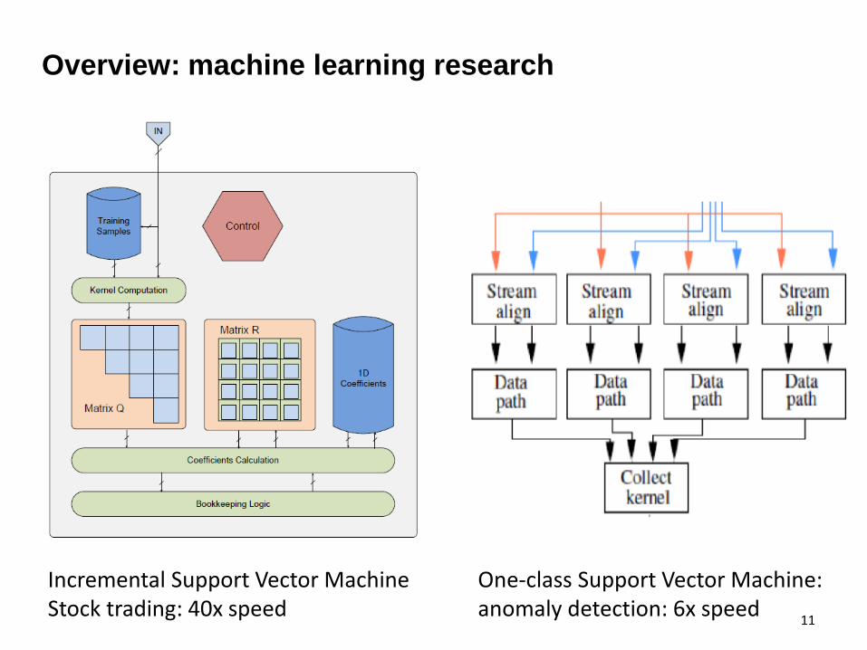
Overview: machine learning research

11

Incremental Support Vector Machine Stock trading: 40x speed

One-class Support Vector Machine: anomaly detection: 6x speed

Overview: machine learning research

12

Pipelined genetic propagation Travelling Salesman: 90x speed

Genetic programming Trading strategy: 3.5x returns

Overview: machine learning research

13

Inductive logic programming Mutagenesis: 30x speed

Sequential Monte Carlo Air traffic management: 5x aircraft

14

2. Example: remote sensing with hyperspectral imaging

Source: http://www.markelowitz.com/Hyperspectral.html

• spectral bands > 200 • Image data > 50GBps • downlink < 10Gbps

15

HyperSpectral image classification

Multiple sensor images One image Spectrum curve Pixel

Data cube Pseudo color image

Large computation under strict power constraint: 30Gops/s @20W

3. Accelerator design: why SVM classification?

16

Source: https://en.wikipedia.org/wiki/Support_vector_machine

2D Case H1 does not separate the classes. H2 does, but only with a small margin. H3 separates them with the maximum margin. SVM covers higher dimensions: hyperplanes.

1 vs 2 1vs3 7vs8

Voting

Not1 1vs4

2vs4 1vs3

3vs4 2vs3 1vs2

Not4

Not2 Not1 Not4

Not3

K(K-1)/2 K(K-1)/2 K-1

3. Accelerator design: multi-class SVM classifiers

17

1 vs all

2 vs all

K-1 vs all

Judge

One-Against-One One-Against-All Directed Acyclic Graph

• each class: possible interpretation of image pixel data • One-Against-One: higher accuracy when used with Hamming Distance

1 vs 2 1 vs 3 (K-1) vs K

Judge

OAO Multiple classifiers with Hamming Distance

0 1 2 T

0 1 2 T Hamming Distance 0 1 2 T

Class 1 ID

0 1 2 T

Class 2 ID

Class K ID

T+1 = K×(K-1)/2

Binary Classifiers (BC)

Hamming code

Class label

Image data

Hamming Distance of 2 strings: number of corresponding positions that are different. Compare 1 vs 2, 1 vs 3… results with an Identifying Code for Class 1; small Hamming Distance: image data pixel is in this class

from training

Pseudo code for multi class SVM classifier

19

Radial basis function

hyper- parameters, found by training

(Identify each class) (treat X as 0)

Accelerator Architecture

20 BC： Binary Classifier

Binary Classifier: datapath of kernel

21

Radial basis function

hyper- parameters, found by training

Evaluation

22

• hardware platform

• data sets

- Maxeler MAX4 DFE - Altera Stratix V 5SGSMD8N2F45C2 FPGA

- Airborne Visible Infra-Red Imaging Spectrometer (AVIRIS), Northwestern Indiana scene and Salinas Valley scene - 224 spectral bands - 16 classes

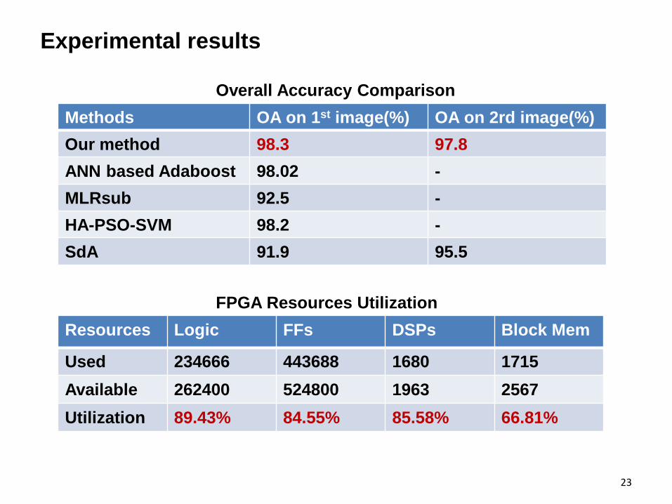
Experimental results

Methods OA on 1st image(%) OA on 2rd image(%) Our method 98.3 97.8 ANN based Adaboost 98.02 - MLRsub 92.5 - HA-PSO-SVM 98.2 - SdA 91.9 95.5

Overall Accuracy Comparison

Resources Logics FFs DSPs Block Mem

Used 234666 443688 1680 1715 Available 262400 524800 1963 2567 Utilization 89.43% 84.55% 85.58% 66.81%

FPGA Resources Utilization

23

Runtime and energy consumption comparison

Platform Zynq ARM DSP Xeon DFE T(μs/Pixel) 25.8 1321.2 65.8 14.1 0.99

Power(W) 3.9 3.3 16 95 26.3

E(mJ/Pixel) 0.1 4.3 1.05 1.33 0.03 Speedup 26.0 1334.5 66.4 14.2 1

• Zynq: XC7Z020 • ARM: Cortex A9 @667MHz • DSP: TMS320C6678 8 cores@1GHz • Xeon: Inter E5-2620 12cores, OpenMP optimized • DFE Running frequency: 120MHz • 8 Millions Pixels for Xeon test and 1 Million Pixels for others

24

25

• assertions – Boolean expressions – when true, circuit is behaving correctly – in-circuit: runs at same rate as rest of design – propagate to software as extra outputs

• exceptions – like software exceptions: allow errors to be handled – can replace erroneous value with safe one

4. Monitoring: in-circuit assertions and exceptions

26

Example: statistical assertions

• in-circuit – runs at user circuit speed – allows rapid self-adaptive hardware + software

• statistical

– adaptation can depend on signal statistics – assertion language e = a | uop e | e bop e | mean(e) | variance(e) | …

• implementation

– feedforward and feedback architectures of pairwise and linear algorithms

– allows more user choice in speed / area tradeoff

27

Statistical assertion: self-adaptive system

28

Case study: smart avionics

• air-speed sensor: Pitot tube • can fail when frozen

could still fail

29

True airspeed: statistical check

• true airspeed: important input to avionics • statistics on true airspeed: indicate sensor failure

– trigger self-adaptation • true airspeed datapath for sensor

– monitored by in-circuit variance operators

datapath

30

Assertion: resource required

• modest linear area cost per in-circuit assertion • calculate airspeed within hard real-time limit

31

Assertions: efficient implementation

• properties to be monitored – functional – statistical – timing

• run-time hardware monitoring – high-level description: assertion – same speed as hardware to be monitored – provably-correct optimisation – minimum area overhead: O(N) -> O(logN)

32

• obvious (S = )

• efficient

• proof: use algebraic transformations in Ruby language

Optimising assertion: correctness-preserving transformation

33

Assertions: efficient implementation

• properties to be monitored – functional – statistical – timing

• run-time hardware monitoring – high-level description: assertion – same speed as hardware to be monitored – provably-correct optimisation – minimum area overhead: O(N) -> O(logN)

34

Assertions: efficient implementation

• properties to be monitored – functional – statistical – timing

• run-time hardware monitoring – high-level description: assertion – same speed as hardware to be monitored – provably-correct optimisation – minimum area overhead: O(N) -> O(logN) -> O() – minimise compile time

35

Self-monitoring without overhead

• add monitoring to user design – introduce new circuit – without modifying user design – use only spare resources on chip

• accelerate monitoring circuit – pipeline its input connections

36 36

New design flow: resource-aware implementation

(XDL)

37

Self-monitoring circuitry: results

• pipeline circuits to added hardware to reduce / eliminate impact on timing

• up to 3.9 times faster on large circuits (LEON3 CPU) than re-compilation

Assertion: PC in range Assertion: statistics of AES output

38

Summary

• current and future work – tools: automate implementation and verification – applications: adaptive and resilient systems – extension: assertion management and optimisation – unification: with self-tuning control, self-aware systems… – prototyping: next-generation satellites, planes, drones…

39

Summary

• current and future work – tools: automate implementation and verification – applications: adaptive and resilient systems – extension: assertion management and optimisation – unification: with self-tuning control, self-aware systems… – prototyping: next-generation satellites, planes, drones…

• future smart sensing systems: field-programmable technology – machine learning: self-optimisation – assertion-based monitoring: self-verification – resource-aware implementation: reduced overhead