TR2007-117 July 2007 ACM Transactions on Graphics · TR2007-117 July 2007 Abstract We describe a method for converting time-lapse photography captured with outdoor cameras into Factored

MITSUBISHI ELECTRIC RESEARCH LABORATORIEShttp://www.merl.com

Factored Time-Lapse Video

Kalyan Sunkavalli, Wojciech Matusik, Hanspeter Pfister, Szymon Rusinkiewicz

TR2007-117 July 2007

Abstract

We describe a method for converting time-lapse photography captured with outdoor camerasinto Factored Time-Lapse Video (FTLV): a video in which time appears to move faster (i.e.,lapsing) and where data at each pixel has been factored into shadow, illumination, and reflectancecomponents. The factorization allows a user to easily relight the scene, recover a portion ofthe scene geometry (normals), and to perform advanced image editing operations. Our methodis easy to implement, robust, and provides a compact representation with good reconstructioncharacteristics. We show results using several publicly available time-lapse sequences.

ACM Transactions on Graphics

This work may not be copied or reproduced in whole or in part for any commercial purpose. Permission to copy in whole or in partwithout payment of fee is granted for nonprofit educational and research purposes provided that all such whole or partial copies includethe following: a notice that such copying is by permission of Mitsubishi Electric Research Laboratories, Inc.; an acknowledgment ofthe authors and individual contributions to the work; and all applicable portions of the copyright notice. Copying, reproduction, orrepublishing for any other purpose shall require a license with payment of fee to Mitsubishi Electric Research Laboratories, Inc. Allrights reserved.

Copyright c©Mitsubishi Electric Research Laboratories, Inc., 2007201 Broadway, Cambridge, Massachusetts 02139

MERLCoverPageSide2

ACM Reference FormatSunkavalli, K., Matusik, W., Pfi ster, H., Rusinkiewicz, S. 2007. Factored Time-Lapse Video. ACM Trans. Graph. 26, 3, Article 101 (July 2007), 10 pages. DOI = 10.1145/1239451.1239552 http://doi.acm.org/10.1145/1239451.1239552.

Copyright NoticePermission to make digital or hard copies of part or all of this work for personal or classroom use is granted without fee provided that copies are not made or distributed for profi t or direct commercial advantage and that copies show this notice on the fi rst page or initial screen of a display along with the full citation. Copyrights for components of this work owned by others than ACM must be honored. Abstracting with credit is permitted. To copy otherwise, to republish, to post on servers, to redistribute to lists, or to use any component of this work in other works requires prior specifi c permission and/or a fee. Permissions may be requested from Publications Dept., ACM, Inc., 2 Penn Plaza, Suite 701, New York, NY 10121-0701, fax +1 (212) 869-0481, or [email protected].© 2007 ACM 0730-0301/2007/03-ART101 $5.00 DOI 10.1145/1239451.1239552 http://doi.acm.org/10.1145/1239451.1239552

Factored Time-Lapse Video

Kalyan Sunkavalli∗ Wojciech Matusik†

MERLHanspeter Pfister‡ Szymon Rusinkiewicz§

Princeton University

(a) Original (b) Reconstructed, no shadows (c) Sun illumination only (d) Modified reflectanceFigure 1: We decompose a time-lapse sequence of photographs (a) into sun, sky, shadow, and reflectance components. The representationpermits re-rendering without shadows (b) and without skylight (c), or modifying the reflectance of surfaces in the scene (d).

Abstract

We describe a method for converting time-lapse photographycaptured with outdoor cameras into Factored Time-Lapse Video(FTLV): a video in which time appears to move faster (i.e., lapsing)and where data at each pixel has been factored into shadow, illumi-nation, and reflectance components. The factorization allows a userto easily relight the scene, recover a portion of the scene geometry(normals), and to perform advanced image editing operations. Ourmethod is easy to implement, robust, and provides a compact repre-sentation with good reconstruction characteristics. We show resultsusing several publicly available time-lapse sequences.

CR Categories: I.4.8 [Image Processing and Computer Vision]:Scene Analysis—Time-varying Imagery I.3.7 [Computer Graph-ics]: Three-Dimensional Graphics and Realism—Color, shading,shadowing, and texture

Keywords: Image-based rendering and lighting, inverse problems,computational photography, reflectance

1 Introduction

Time-lapse photography, in which frames are captured at a lowerrate than that at which they will ultimately be played back, datesback to the late 19-th century1. Classic time-lapse photography

∗e-mail: [email protected]†e-mail:[email protected]‡e-mail:[email protected]§e-mail:[email protected]

1Georges Melies’ motion picture Carrefour De L’Opera (1897)(wikipedia.org)

subjects are clouds, stars, plants, and flowers. Today, most time-lapse image sequences are collected by the thousands of cameras(webcams) whose images can be accessed using the Internet. Theytypically provide outdoor views of cities, construction sites, traffic,the weather, or natural phenomena such as volcanoes. Outdoor we-bcams are also used for surveillance to monitor outside activitiesaround companies, ports, or warehouses. So-called webcam direc-tories index thousands of live webcams, providing instant onlineaccess to time-lapse photos from around the world.

Time-lapse photography can create an overwhelming amount ofdata. For example, a single camera that takes an image every 5seconds will produce 17,280 images per day, or close to a millionimages per year. Image or video compression reduces the storagerequirements, but the resulting data has compression artifacts andis not very useful for further analysis. In addition, it is currentlydifficult to edit the images in a time-lapse sequence, and advancedimage-based rendering operations such as relighting are impossi-ble. A key challenge in dealing with time-lapse data is to providea representation that efficiently reduces storage requirements whileallowing useful scene analysis and advanced image editing.

In this paper we focus on time-lapse sequences of outdoor scenesunder clear-sky conditions. The camera viewpoint is fixed andthe scene is mostly stationary, hence the predominant changes inthe sequence are changes in illumination. Under these assump-tions we have developed a method that provides a complete de-composition of the original dataset into shadow, illumination, andreflectance components. We call this representation Factored Time-Lapse Video (FTLV).

Our method begins by locating the onset of shadows using thetime-varying intensity profiles at each pixel. We identify pointsin shadow and points in direct sunlight to separate skylight andsunlight components, respectively. We then analyze these spatio-temporal volumes using matrix factorization. The results are basiscurves describing the changes of intensity over time, together withper-pixel offsets and scales of these basis curves, which capture spa-tial variation of reflectance and geometry. The resulting represen-tation is compact, reducing a time-lapse sequence to three images,two basis curves, and a compressed representation for shadows. Re-constructions from the data show better error characteristics thanstandard compression methods such as PCA.

FTLVs are an intrinsic image-like scene representation that allow auser to analyse, reconstruct and modify illumination, reflectance, or

ACM Transactions on Graphics, Vol. 26, No. 3, Article 101, Publication date: July 2007.

geometry. The shadows may be discarded or retained, dependingon the ultimate application, while other “outliers” such as pedes-trians or cars are implicitly ignored. FTLVs can also be used forvarious computer vision tasks such as background modeling, imagesegmentation, and scene reconstruction. In this paper we demon-strate several applications for FTLVs, including relighting, shadowremoval, advanced image editing, and pictorial rendering.

2 Previous Work

Time-Lapse Sequence Analysis Barrow and Tenen-baum [1978] introduced the concept of intrinsic images torepresent intrinsic characteristics of a scene, such as illumination,reflectance, and surface geometry. Weiss [2001] uses a maximum-likelihood framework to estimate a single reflectance image andmultiple illumination images from time-lapse video. His workwas extended by Matsushita et al. [2004] who derive time-varyingreflectance and illumination images from surveillance video.

Matusik et al. [2004] use time-lapse data to compute the reflectancefield (or light transport) of a scene for a fixed viewpoint. Theyrepresent images as a product of the reflectance field and the in-coming illumination. However, the method requires estimating theincident illumination using a light probe camera, and the estimatedreflectance field combines the effects of reflectance and shadows.

Koppal and Narasimhan [2006] acquire image sequences with arandomly moving light source to cluster the image into regions thathave similar normals. These normal clusters are then used as priorsto bootstrap a variety of vision algorithms, including the decom-position of the image into the terms of a linearly separable BRDFmodel. Because the illumination is required to follow an unstruc-tured trajectory, Koppal and Narasimhan’s work is applicable onlyto outdoor time-lapse data captured over a larger period of time(many days or weeks).

Unlike this previous work, we arrive at a decomposition of time-lapse sequences into shadows, partial scene geometry, and time-varying reflectance and illumination. This provides better estimatesof intrinsic image qualities and more accurate scene analysis.

Reflectance Factorizations Lawrence et al. [2006] describe afactorization method to decompose complex surface reflectancefunctions (spatially varying BRDFs) into a sum of products of lowerdimensional (1D or 2D) terms. Similarly, Gu et al. [2006] decom-pose a time-varying surface appearance into lower dimensional rep-resentations that are space-time dependent. Both of these methodsaccomplish similar goals — they factorize large datasets of com-plex surface reflectances into terms that are highly compact and atthe same time physically meaningful and editable. Since they ac-quire and model the full eight-dimensional BRDF they can renderunder any viewing, lighting, and, in the case of Gu et al.[2006],temporal condition. However, the complexity of the BRDF acqui-sition setup makes it impractical for complex, outdoor scenes.

Our work bridges the gap between intrinsic images and the factor-ization of complex reflectance functions. In doing so we go beyondthe mid-level representation of intrinsic images without requiringthe acquisition setup and calibration of a complete BRDF estima-tion.

Inverse Rendering Inverse rendering measures rendering at-tributes — lighting, textures, and BRDF — from photographs. Al-though there is prolific literature on inverse rendering, most of thework focuses on small objects and indoor scenes. Yu and Ma-lik [1998] and Debevec et al. [2004] recover photometric propertiesfrom photographs of outdoor architectures. They are able to relight

them and create photo-realistic images from arbitrary viewpoints.However, their methods require measurements of the incident illu-mination and surface materials and a 3D model of the scene geom-etry. Similarly, Nimeroff et al. [1994] render scenes under naturalillumination by combining basis images that are pre-rendered usinga set of basis illuminations. But they also require measurements ofscene geometry and reflectances.

Seitz et al. [2005] and Nayar et al. [2006] separate the illumina-tion in a scene into its direct and global components using con-trolled lighting. They demonstrate this for real-world materials andcomment on the contribution of the two terms to surface appear-ance. We separate illumination into a global sky and a direct suncomponent while ignoring secondary inter-reflections, scattering,or translucency.

Video Analysis and Editing There has been considerable re-search on analyzing video sequences to segment out objects andextract mattes [Chuang et al. 2002; McGuire et al. 2005; Li et al.2005; Wang et al. 2005], to extract shadows [Chuang et al. 2003],to determine object motion and texture [Bregler et al. 1997; Schodlet al. 2000; Bhat et al. 2004], and to combine video frames intopanoramas [Agarwala et al. 2005]. In addition, there has been re-cent work that modifies video by inserting objects [Li et al. 2005;Wang et al. 2005] or shadows [Chuang et al. 2002], enhancingsmall motion [Liu et al. 2005], or applying non-photorealistic styl-ization [Litwinowicz 1997; Wang et al. 2004; Winnemoller et al.2006]. In contrast, the present paper performs a different type ofanalysis, focusing not on inferring objects’ shape, motion, or tex-ture, but rather on decomposing appearance and reflectance. Ouranalysis enables a different class of edits, such as changing re-flectance and lighting. In addition, by extracting partial geometry ofthe scene, we are able to perform stylization using algorithms suchas exaggerated shading [Rusinkiewicz et al. 2006], which requiresmore knowledge about the scene than simply pixel intensities.

3 Representation

Our goal is to decompose the space-time volume F(t) of the time-lapse image sequence into factors that will enable us to analyze andedit the scene. As the sun moves, the observations at every pixelin the time-lapse sequence result in a continuous appearance pro-file [Koppal and Narasimhan 2006] (see Figure 4(a)). The appear-ance profile (red curve) is a vector of intensities Fi(t) measured atpixel Pi over time (i.e., frame number). It is a complicated functionof the illumination, scene geometry, and surface reflectance.

Under the clear-sky assumption we can approximate the illumina-tion as a sum of an ambient term corresponding to sky illuminationand a single-directional light source corresponding to the radianceof the sun. Using the linearity of the rendering equation, the spatio-temporal volume F(t) can therefore be expressed as a sum of thesky light and sunlight components:

F(t) = Isky(t) + Ssun(t) ∗ Isun(t). (1)

Here Ssun(t) is the shadowing term that describes if a pixel is inshadow (and therefore has no sunlight contribution) or not.

One of the key insights in this paper is that for outdoor time-lapse sequences under clear-sky conditions the appearance pro-files of all points in the scene are similar up to an offset alongthe time axis and a scale factor. This is similar to the notion oforientation-consistency introduced by Hertzmann and Seitz [2005],which states that, under the right conditions, two points with thesame surface orientation must have the same or similar appearance

101-2 • Sunkavalli et al.


Figure 2: An overview of the FTLV factorization. We separate thespatio-temporal volume (a) F(t) into the sky component (b) Isky(t)and the sun component (d) Isun(t) modulated by the shadow vol-ume (c) S(t). The sky component is factorized into (e) per-pixelweights Wsky and a time-curve Hsky(t) while the sun componentis factorized into (f) albedo Wsun(t), reflectance Hsun(t) and per-pixel shifts S(t).

in an image. They compute the surface normals of a target ob-ject that has been imaged together with one or more reference ob-jects with known shape (sphere) and similar BRDF. Koppal andNarasimhan [2006] also noted that scene points with the same sur-face normal often exhibit extrema in their profiles at the same timeinstant, irrespective of their material properties. They use a metricthat matches appearance profile extremas, and unsupervised clus-tering, to compute orientation consistencies between scene pointsof unknown normals and BRDFs. The key difference in our work isthat we seek to separate the contributions of shadows, skylight, andsun illumination. Similar to the work by Gu et al. [2006], we repre-sent the corresponding appearance profiles as a linear combinationof basis curves that are offset and scaled.

Based on our insight, we approximate Isun(t) with a single basiscurve Hsun(t) scaled by per-pixel weights Wsun. In addition, weallow a per-pixel time offset Φ to the sunlight curve that stands infor the normal dependence of the appearance profile:

Isun,i(t) ≈ Wsun,i Hsun(t + Φi). (2)

We call weight matrix Wsun the sunlight image, the basis curveHsun(t) the sunlight basis curve and the offset Φ the shift map.Since the sun is a strong directional light source, Hsun(t) is anestimate of the 1-D slice of surface reflectance corresponding to thecamera viewpoint and the arc described by the sun’s motion.

The time-shifted basis is an accurate representation for appearanceprofiles because of the nature of sun illumination. Since the sunmoves at a constant angular velocity, the appearance profiles at pix-els with different surface normals correspond to different uniformlysampled 1-D slices (corresponding to the camera viewpoint and theplane of the sun) of the 4-D BRDF. For both diffuse and specularsurfaces it has been shown that the shape of this slice is largely thesame with the fundamental difference being the normal-dependentshift that Φ captures. If the arc described by the sun is known, un-der the assumption that the appearance profile is maximum whenthe sunlight is normally incident on the surface, the computed shiftmap can be converted into an estimate of the surface normal. Sincethe sun moves only in a plane, the shift map is an estimate of thesurface normal projected onto this plane.

In order to estimate Isky(t) in Equation (1), we look to find a sin-gle illumination-vs.-time basis curve Hsky(t) for the entire imagesequence, such that the appearance of any shadowed pixel Pi maybe reproduced as:

Isky,i(t) ≈ Wsky,i Hsky(t). (3)

We call the matrix Wsky of per-pixel weights the skylight image,and the basis curve Hsky(t) the skylight basis curve. Note that wedo not apply an offset to the skylight curve in Equation (3) becausethe diffuse nature of sky illumination makes the offset hard to esti-mate.

The final representation (see Figure 2) therefore is:

F(t) ≈ Wsky Hsky(t) + Ssun(t) ∗Wsun Hsun(t + Φ). (4)

Our goal is to separate F(t) into Isky(t), Ssun(t), and Isun(t) andestimate all the per-pixel weights, per-pixel shifts, and time-curveswithout knowledge of scene geometry, reflectance, illumination, orcamera calibration. We make the observation that we can estimateIsky(t) from points that are in shadow, whereas points in the suncontain Isky(t)+Isun(t). Our approach is to first estimate Ssun(t)and to use this to separate Isky(t) and Isun(t) and estimate the restof the terms. The next section describes how we estimate Ssun(t)from the time-lapse data, and Section 5 shows how we use matrixfactorization to solve for Wsky , Hsky(t), Wsun, Φ and Hsun(t).

4 Shadow Estimation

Figure 3 shows one frame of a time-lapse sequence of the SantaCatalina Mountains in Arizona. We will use this frame and pixelsA, B, and C throughout our discussion. All computations are per-formed in RGB color space and independently on the three colorchannels. For simplicity we will focus on the red channel only.

Figure 3: Frame 275 of the Arizona time-lapse sequence.

Our model assumes that the color of visible pixels is due to reflec-tion from surfaces in the scene. Therefore we do not consider skypixels in our representation. We compute the sky mask (using Pho-toshop’s magic wand tool) for one frame and use it to later compos-ite the sky from the original data to the reconstructed images. Thishas the added benefit that we preserve moving clouds, which are animportant visual component in time-lapse videos.

As can be seen in Figure 4(a) pixel intensities differ dramatically ifthe scene point is illuminated by the sun or if it is in shadow. We usethese discontinuities in the appearance profiles to estimate shadowimages. We first compute the median value mmin of the n smallestintensities at each pixel. We typically assume that each point is inshadow at least 20% of the time, so n is 20% of the total number offrames in the sequence. We set the shadow function Si(t) (purplecurve in Figure 4(a)) to one for each Fi(t) > kmmin and to zerootherwise. We heuristically found that k = 1.5 worked well formost of the sequences in our experiments.

Figure 5 (top) shows the value of the shadow function for all pixelsin frame 275. We call this the binary shadow image. It is gener-ally quite noisy due to moving objects (e.g., trees, smoke, or peo-ple) and changes in the illumination (e.g., clouds). Therefore, tocompute the final shadow image Ssun we use an edge-preservingbi-lateral filter [Tomasi and Manduchi 1998] (Figure 5 (bottom)).We could improve the shadow images by explicitly removing dy-namic objects, either by computing median images for short time

Factored Time-Lapse Video • 101-3


(a) (b) (c) (d)

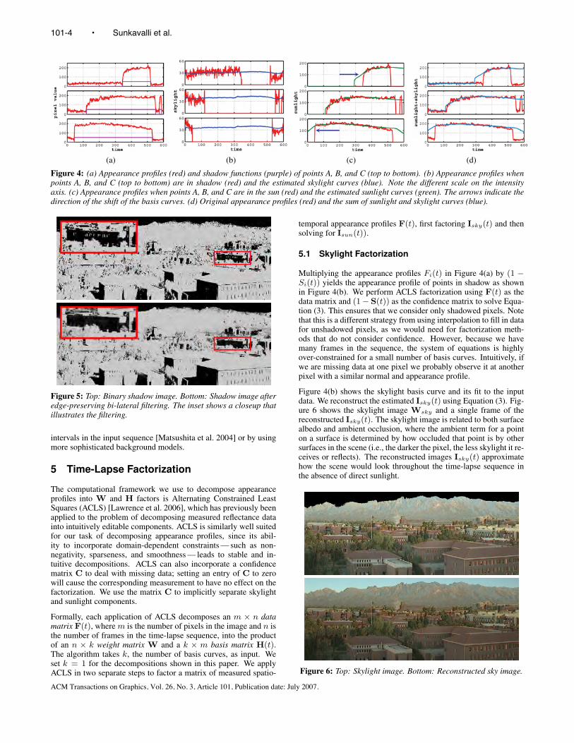
Figure 4: (a) Appearance profiles (red) and shadow functions (purple) of points A, B, and C (top to bottom). (b) Appearance profiles whenpoints A, B, and C (top to bottom) are in shadow (red) and the estimated skylight curves (blue). Note the different scale on the intensityaxis. (c) Appearance profiles when points A, B, and C are in the sun (red) and the estimated sunlight curves (green). The arrows indicate thedirection of the shift of the basis curves. (d) Original appearance profiles (red) and the sum of sunlight and skylight curves (blue).

Figure 5: Top: Binary shadow image. Bottom: Shadow image afteredge-preserving bi-lateral filtering. The inset shows a closeup thatillustrates the filtering.

intervals in the input sequence [Matsushita et al. 2004] or by usingmore sophisticated background models.

5 Time-Lapse Factorization

The computational framework we use to decompose appearanceprofiles into W and H factors is Alternating Constrained LeastSquares (ACLS) [Lawrence et al. 2006], which has previously beenapplied to the problem of decomposing measured reflectance datainto intuitively editable components. ACLS is similarly well suitedfor our task of decomposing appearance profiles, since its abil-ity to incorporate domain-dependent constraints — such as non-negativity, sparseness, and smoothness — leads to stable and in-tuitive decompositions. ACLS can also incorporate a confidencematrix C to deal with missing data; setting an entry of C to zerowill cause the corresponding measurement to have no effect on thefactorization. We use the matrix C to implicitly separate skylightand sunlight components.

Formally, each application of ACLS decomposes an m × n datamatrix F(t), where m is the number of pixels in the image and n isthe number of frames in the time-lapse sequence, into the productof an n × k weight matrix W and a k × m basis matrix H(t).The algorithm takes k, the number of basis curves, as input. Weset k = 1 for the decompositions shown in this paper. We applyACLS in two separate steps to factor a matrix of measured spatio-

temporal appearance profiles F(t), first factoring Isky(t) and thensolving for Isun(t)).

5.1 Skylight Factorization

Multiplying the appearance profiles Fi(t) in Figure 4(a) by (1 −Si(t)) yields the appearance profile of points in shadow as shownin Figure 4(b). We perform ACLS factorization using F(t) as thedata matrix and (1− S(t)) as the confidence matrix to solve Equa-tion (3). This ensures that we consider only shadowed pixels. Notethat this is a different strategy from using interpolation to fill in datafor unshadowed pixels, as we would need for factorization meth-ods that do not consider confidence. However, because we havemany frames in the sequence, the system of equations is highlyover-constrained for a small number of basis curves. Intuitively, ifwe are missing data at one pixel we probably observe it at anotherpixel with a similar normal and appearance profile.

Figure 4(b) shows the skylight basis curve and its fit to the inputdata. We reconstruct the estimated Isky(t) using Equation (3). Fig-ure 6 shows the skylight image Wsky and a single frame of thereconstructed Isky(t). The skylight image is related to both surfacealbedo and ambient occlusion, where the ambient term for a pointon a surface is determined by how occluded that point is by othersurfaces in the scene (i.e., the darker the pixel, the less skylight it re-ceives or reflects). The reconstructed images Isky(t) approximatehow the scene would look throughout the time-lapse sequence inthe absence of direct sunlight.

Figure 6: Top: Skylight image. Bottom: Reconstructed sky image.



(a) Temple (b) Square (c) Tokyo (d) Yosemite

Figure 7: Example frames for each dataset (first row) and appearance profiles (second row) of pixels A, B, and C (red channel). In the thirdrow are the aligned appearance profiles and estimated sunlight basis curves (black). The profiles were aligned and scaled using the estimatedshifts Φi and Wsun for pixels A, B, and C.

5.2 Sunlight Factorization

The reconstructed images Isky(t) are subtracted from the origi-nal data F(t) and the result is clamped to 0 to form the matrixIsun(t). Multiplying Isun,i(t) by Si(t) yields the appearance pro-file of frames when the points are illuminated only by sunlight asshown in Figure 4(c). Using Isun(t) as the data matrix and S(t) asthe confidence matrix C thus ensures that only the sunlight compo-nent at every pixel is considered during the factorization. We runACLS to solve Equation (2) and compute the basis curve Hsun, thesunlight image Wsun, and the shifts Φi.

In order to adapt ACLS to handle the time-offsets necessary to im-plement Equation (2), we modify the iterative update stage of thealgorithm. Specifically, the original algorithm alternates betweenphases in which H(t) is held fixed while W is optimized usingleast squares, then vice versa (this is an instance of the principle ofexpectation maximization in inference). In order to incorporate theshifts Φi, we shift the entire matrix H(t) by +Φi when updatingWi and, similarly, shift each row i of F(t) by −Φi during updatesof H(t). Finally, we introduce a third update phase during the it-eration, in which we update Φi by finding, for each pixel, the shiftthat minimizes error. The metric used here is the same as that forupdating W and H, i.e., the confidence-weighted Euclidean errorbetween the scaled and offset basis curve H(t) and F(t). As withACLS, our modified algorithm reduces error at each iteration, andis guaranteed to converge to a (possibly local) minimum.

Figure 4(c) shows the sunlight basis curve Hsun(t) and its fit tothe input data, and Figure 8 shows the sunlight image Wsun andthe reconstructed image Isun(t). The harsh black shadows in thereconstructed image Isun(t) are similar to images taken in a vac-uum without atmospheric light scattering, such as images from themoon. Figure 8 (bottom) shows the shifts Φ for the sun component.This image is a good estimate of the partial geometry (normals) of

Figure 8: Top: Sunlight image. Middle: Reconstructed sun image.Bottom: Shift map.

the scene. If we have time-lapse sequences from the same staticviewpoint for different days, it is possible to recover more than justthis one-dimensional approximation of surface normals.



(a)

(b)

(c)

Figure 9: Original images (a) of the Square sequence compared to our reconstruction with (b) and without shadows (c).

6 Results

The datasets for our experiments come from online webcams 2. Asshown in Table 1, the sequences are of varying length and resolu-tions, typically captured at intervals in the range of every 15 sec-onds to every 5 minutes. All of the datasets were originally com-pressed. We extracted the individual frames and automatically re-moved the regions covered by the sky using the sky-mask. All re-sults in this paper and video were computed without sky. For someof the results in the paper and the video we composited the skyregions back into the sequences.

6.1 Reconstruction Quality

Figure 7 shows sample images from four sequences with three pix-els marked on each. The figure shows the appearance profiles forthe red channel of the pixels over time (similar results are obtainedfor green and blue). Similar to Figure 4, the profiles show shad-owing in the form of discontinuities but otherwise appear similar toeach other. In Figure 7 in the bottom row we show the alignmentof these separate time-varying profiles using the scales Wsun,i andshifts Φi we estimated in our factored representation for each pixel.The black curves show the sunlight basis curves for each sequence.The scaled and time-shifted profiles match the basis curves verywell.

Figure 9 qualitatively shows the accuracy of our reconstruction forthe Square sequence. The reconstruction with shadows accuratelymatches the original images. Specific problem areas in this se-quence are the streets and sidewalks due to parked cars, movingtraffic, and people. Interestingly, our shadow estimation techniquepicks up the shadows of moving objects, which are especially vis-ible in a few of the sequences shown in the accompanying video.

2Data courtesy of: Santa Catalina Mountains, Arizona - Dec 5 2006(http://www.cs.arizona.edu/camera); Nauvoo Temple. Illinois - Dec 102002 (http://deseretbook.com/nauvoo/archive); Yosemite: Half-dome fromGlacier Point - Dec 19 2006 (http://www.halfdome.net/); Tokyo RiversideSkyline - Jan 08 2007 (http://tokyosky.to/).

In some cases we median-filtered the shadows Ssun(t) temporallyto remove flickering due to moving people, cars, etc. The bottomrow in the figure shows our reconstruction without shadows. It ef-fectively removes the “ghost” shadows of moving objects and thelarge shadow that is visible throughout most of the sequence.

6.2 Error Analysis

Table 1 shows the overall RMS image reconstruction errors forFTLV that were computed across all temporal frames and spatiallocations. The error is quite large compared to traditional imageand video compression. This is not surprising, since FTLV doesnot encode moving objects. To get a better qualitative handle onthe reconstruction error we compare FTLV to principal componentanalysis (PCA), a standard matrix rank-reduction algorithm. Simi-lar to ACLS, PCA decomposes the original spatio-temporal matrixF into the sum of the mean F and a product of weight matrices Wand basis vectors H. The number of basis vectors determines thefidelity of the reconstruction.

Figure 10 shows a plot of the PCA RMS reconstruction error versusthe number of PCA terms for each of our sequences. We indicate

Figure 10: PCA RMS reconstruction error vs. number of PCAterms. The symbol X indicates the RMS error of FTLV.



Dataset # Imgs Resolution RMS Error PCA Terms Raw PCA FTLV w/o FTLV +Shadows Shadows

Arizona 610 720× 278 14.5% 5 + 1 350 MB 1,118 kB 475 kB 1,665 kBTemple 590 464× 355 13.7% 2 + 1 278 MB 63 kB 40 kB 541 kB

Yosemite 293 480× 360 10.1% 8 + 1 115 MB 1,040 kB 297 kB 2,289 kBTokyo 380 920× 612 15.9% 4 + 1 353 MB 1,200 kB 868 kB 3,601 kBSquare 850 648× 330 12.2% 4 + 1 441 MB 815 kB 765 kB 1,257 kB

Table 1: Datasets and file sizes. Sky pixels were removed from the Raw and PCA estimates for fair comparison with FTLV.

Figure 11: Closeup of a frame in the Arizona sequence. Top: Orig-inal image. Middle: FTLV reconstruction with 14.5% RMS error.Bottom: PCA reconstruction with the same error using five termsplus the mean. Note the blurry shadows in the PCA reconstruction.

the corresponding FTLV error by the symbol X. The number ofPCA terms that are necessary to achieve the same FTLV RMS erroris also shown in Table 1. PCA typically needs more terms (plus themean) since FTLV is equivalent to three terms (images). A visualcomparison of the corresponding reconstructed sequences showsthat FTLV is more effective in preserving sharp details, especiallyat shadow boundaries (see Figure 11). A reasonable reconstruc-tion of shadows requires a large number of PCA terms (at least 15for our datasets). In addition, PCA does not produce a meaningfuldescription of the data. In particular, PCA allows negative valuesin W and H, resulting in a representation whose terms cannot beedited independently.

6.3 Compression

As can be seen from Table 1, FTLV is a highly compact and efficientrepresentation for time-lapse sequences. For these comparisons,we store the skylight, sunlight, and shift images using high-qualityJPEG. The binary shadow functions are stored per pixel. For eachpixel, we store the frame numbers at which shadows start and endand do LZW compression on these number-pairs. The two basis

curves are stored in ASCII text files. Table 1 shows the file sizes forraw images, PCA, FTLV without shadows, and FTLV with shad-ows. The file size of FTLVs is dominated by the encoded shadows.Of course this is very scene dependent. Scenes with highly complexshadows (pixels go in and out of shadow many times) have multi-ple shadow start-end pairs and this is why scenes such as Yosemiterequire more storage while Temple or Square require less.

6.4 Editing and NPR

A major benefit of FTLV is that it factors the scene into physicallymeaningful components, each of which can be edited to create in-teresting effects. Edits to the shift image affect surface appearanceby changing their pseudo-normals. An example of this can be seenin Figure 12, where we show closeups of three frames from theYosemite sequence. We added the imprint of the SIGGRAPH logoto the snow in the foreground by editing the shift map. We alsoedited the shadows in that region to keep the logo in sunlight.

Edits to the sunlight image and curve have an effect on surface re-flectance. Figure 1(d) shows an example of this for the Square se-quence. We changed the surface appearance of various rooftops bychanging the sunlight curve to be more specular. We changed thesunlight image to add the SIGGRAPH logo and added windows tothe building in the front by editing the skylight, sunlight, and shifts.We also selectively removed shadows, for example, for the buildingin the background. Note that by simply editing the skylight, sun-light, or shifts we affected the entire time-lapse sequence. As can beseen in the accompanying video, the results look visually plausibleand could certainly be improved with more artistic care.

In order to demonstrate the flexibility of our method, we have alsoexperimented with non-photorealistic effects to generate stylizedimages and videos of the input scenes. We first transform the shiftmaps Φ into pseudo-normal maps by mapping shifts to angles alongan arc through the sky. In order to slightly add to the plausibil-ity of the normals, we apply a small shift to the normals based onthe ratio between the computed sky and sun maps (reasoning thatvertical surfaces generally receive less sky illumination than hor-izontal ones do). While these normals are certainly not accurate,we nevertheless expect that they are related to the true normals bysome (continuous) function, and they are sufficient as input to ren-dering techniques such as exaggerated shading [Rusinkiewicz et al.2006], which seek to emphasize local differences between normals.We generate our final NPR results by compositing the exaggeratedshading with the sun and sky color maps, as well as (optionally)the shadow maps. Figure 13 shows results obtained using this tech-nique for still images, while the supplementary video shows theresult for moving scenes. Note that the computation is temporallycoherent over time, leading to smooth video results (with only sharptemporal discontinuities due to the motion of shadows).



Figure 12: Edits in the Yosemite sequence to add a logo to the snow. The edits were made in the shift (“normal map”) image, and the resultsshow plausible time-varying behavior.

6.5 Discussion

As with any least squares factorization approach there are somepractical considerations to keep in mind while applying FTLV toreal-world data. These are closely tied to the behaviour of the fac-torization and its sensitivity to the various parameters.

6.5.1 Initialization

We have found that in practice FTLV is sensitive to the initial-ization of the shifts Φ but robust to the initialization of W andH. We typically initialize Φ with random values in the range[−(n/2), +(n/2)], where n is the number of frames. This rangemay vary from dataset to dataset and is dependent on the distribu-tion of normals in the scene and the temporal sampling of the data.For example the Square sequence, with a larger span of effectivenormals and temporal sampling, had a larger range. For the Templesequence, which has fewer sets of normals, the range was smaller.

Also, while FTLV is robust to small errors in shadow estimation,drastic errors will corrupt the results. The simple heuristics we useto compute shadows have worked for most of our datasets. Pix-els that are always in the shadows are treated as having Wsun =0 while for pixels that are always in the sun Wsky and Wsun areestimated with additional constraints based on the sunlight and sky-light intensities estimated from other pixels.

6.5.2 Computational Costs

Like the original ACLS algorithm and other least squares optimiza-tions with similarly large amounts of data, FTLV is computationallyintensive. The additional iterations on Φi may be computationallyexpensive (especially if the range of values of Φi that we searchover is very large) but in relative terms do not add significant pro-cessing to the algorithm. Quantitatively, for the Square dataset with180,000 pixels and 850 frames, our sunlight factorization convergesin about 45 mins on a P4 3.0 GHz with 2 GB of RAM.

6.5.3 Sampling

FTLV performance is also dictated by the temporal sampling of theinput time-lapse sequence. The temporal-sampling limitations onour algorithms are closely tied to the nature of scene (diffuse sceneswould work with lower sampling, complex reflectances would re-quire more data points) and camera and image quality (noise, sat-uration, and compression will corrupt data). In our experiments,for the Square dataset (which has fairly smooth and clean appear-ance profiles) we have obtained equivalent results from 60 framesinstead of 850.

7 Conclusions and Future Work

FTLVs are a compact, intuitive, factored representation for time-lapse sequences that separate a scene into its reflectance, illumina-tion, and geometry factors. They enable a number of novel image-based scene modeling and editing applications. The intuitive rep-resentation enables applications such as shadow removal, relight-ing, advanced image editing, and painterly rendering. As sophis-ticated background models FTLVs can be used to model temporalscene variations and improve tracking. Their compact nature en-ables compression of large time-lapse datasets.

While our current results factor scenes into single basis curves it isnot difficult to imagine using multiple curves. Our intuition is thatmultiple basis curves would relate to different material properties(e.g., diffuse and specular curves). This will both reduce error andenable material-based separation of scene elements.

We are currently looking at methods to express images as arbitraryfractional sums of the sky and sun terms. In future work we wouldalso like to extend FTLVs to arbitrary illumination, including in-door scenes, and scenes with participating media, e.g., a time-lapsesequence captured on a foggy day.

Another limitation is that FTLVs do not handle motion. Movingobjects show up in the residue between original and reconstructionand could be added back into the sequence. However, to improvethe FTLV factorization it would be beneficial to remove movingobjects first, or to use an initially computed FTLV as a backgroundmodel for dynamic object tracking and removal. One could thentry to find a compact representation for dynamic scene elements,including clouds and the sky.

8 Acknowledgments

We would like to thank the anonymous reviewers for their insightfulcomments and Jennifer Roderick for proofreading the paper. Szy-mon Rusinkiewicz is supported by the Sloan Foundation and theNational Science Foundation, grant CCF-0347427.

References

AGARWALA, A., ZHENG, K. C., PAL, C., AGRAWALA, M., CO-HEN, M., CURLESS, B., SALESIN, D., AND SZELISKI, R.2005. Panoramic video textures. ACM Trans. on Graph. 24,3, 821–827.

BARROW, H., AND TENENBAUM, J. 1978. Recovering intrinsicscene characteristics from images. Academic Press, 3–26.



BHAT, K., SEITZ, S., HODGINS, J. K., AND KHOSLA, P. 2004.Flow-based video synthesis and editing. ACM Trans. on Graph.23, 3, 360–363.

BREGLER, C., COVELL, M., AND SLANEY, M. 1997. Videorewrite: driving visual speech with audio. In Proc. of ACM SIG-GRAPH, ACM Press, New York, NY, USA, 353–360.

CHUANG, Y.-Y., AGARWALA, A., CURLESS, B., SALESIN,D. H., AND SZELISKI, R. 2002. Video matting of complexscenes. ACM Trans. on Graph. 21, 3 (July), 243–248.

CHUANG, Y.-Y., GOLDMAN, D. B., CURLESS, B., SALESIN,D. H., AND SZELISKI, R. 2003. Shadow matting and com-positing. ACM Trans. on Graph. 22, 3, 494–500.

DEBEVEC, P., TCHOU, C., GARDNER, A., HAWKINS, T.,POULLIS, C., STUMPFEL, J., JONES, A., YUN, N., EINARS-SON, P., LUNDGREN, T., FAJARDO, M., AND MARTINEZ, P.,2004. Estimating Surface Reflectance Properties of a ComplexScene under Captured Natural Illumination. USC ICT TechnicalReport ICT-TR-06.2004.

GU, J., TU, C.-I., RAMAMOORTHI, R., BELHUMEUR, P., MA-TUSIK, W., AND NAYAR, S. 2006. Time-varying surface ap-pearance: acquisition, modeling and rendering. ACM Trans. onGraph. 25, 3, 762–771.

HERTZMANN, A., AND SEITZ, S. M. 2005. Example-based photo-metric stereo: Shape reconstruction with general, varying brdfs.IEEE Trans. on PAMI 27, 8, 1254–1264.

KOPPAL, S. J., AND NARASIMHAN, S. G. 2006. Clustering ap-pearance for scene analysis. In Proc. of CVPR, vol. 2, 1323 –1330.

LAWRENCE, J., BEN-ARTZI, A., DECORO, C., MATUSIK, W.,PFISTER, H., RAMAMOORTHI, R., AND RUSINKIEWICZ, S.2006. Inverse shade trees for non-parametric material represen-tation and editing. ACM Trans. on Graph. 25, 3, 735–745.

LI, Y., SUN, J., AND SHUM, H.-Y. 2005. Video object cut andpaste. ACM Trans. on Graph. 24, 3, 595–600.

LITWINOWICZ, P. 1997. Processing images and video for an im-pressionist effect. In Proc. of ACM SIGGRAPH, ACM Press,New York, NY, USA, 407–414.

LIU, C., TORRALBA, A., FREEMAN, W. T., DURAND, F., ANDADELSON, E. H. 2005. Motion magnification. ACM Trans. onGraph. 24, 3, 519–526.

MATSUSHITA, Y., NISHINO, K., IKEUCHI, K., AND SAKAUCHI,M. 2004. Illumination normalization with time-dependent in-trinsic images for video surveillance. IEEE Trans. on PAMI 26,10, 1336–1347.

MATUSIK, W., LOPER, M., AND PFISTER, H. 2004.Progressively-refined reflectance functions from natural illumi-nation. In Rendering Techniques, Eurographics Association,A. Keller and H. W. Jensen, Eds., 299–308.

MCGUIRE, M., MATUSIK, W., PFISTER, H., HUGHES, J. F.,AND DURAND, F. 2005. Defocus video matting. ACM Trans.on Graph. 24, 3, 567–576.

NAYAR, S. K., KRISHNAN, G., GROSSBERG, M. D., ANDRASKAR, R. 2006. Fast separation of direct and global compo-nents of a scene using high frequency illumination. ACM Trans.on Graph. 25, 3, 935–944.

NIMEROFF, J. S., SIMONCELLI, E., AND DORSEY, J. 1994.Efficient Re-rendering of Naturally Illuminated Environments.

In Fifth Eurographics Workshop on Rendering, Springer-Verlag,Darmstadt, Germany, 359–373.

RUSINKIEWICZ, S., BURNS, M., AND DECARLO, D. 2006. Ex-aggerated shading for depicting shape and detail. ACM Trans.on Graph. 25, 3, 1199–1205.

SCHODL, A., SZELISKI, R., SALESIN, D., AND ESSA, I. 2000.Video textures. In Proc. of ACM SIGGRAPH, ACM Press, NewYork, NY, USA, 489–498.

SEITZ, S. M., MATSUSHITA, Y., AND KUTULAKOS, K. N. 2005.A theory of inverse light transport. In Proc. of ICCV, II: 1440–1447.

TOMASI, C., AND MANDUCHI, R. 1998. Bilateral filtering forgray and color images. In Proc. of ICCV, 839–846.

WANG, J., XU, Y., SHUM, H.-Y., AND COHEN, M. F. 2004.Video tooning. ACM Trans. on Graph. 23, 3, 574–583.

WANG, J., BHAT, P., COLBURN, R. A., AGRAWALA, M., ANDCOHEN, M. F. 2005. Interactive video cutout. ACM Trans. onGraph. 24, 3, 585–594.

WEISS, Y. 2001. Deriving intrinsic images from image sequences.In Proc. of ICCV, II: 68–75.

WINNEMOLLER, H., OLSEN, S., AND GOOCH, B. 2006. Real-time video abstraction. ACM Trans. on Graph. 25, 3, 1221–1226.

YU, Y., AND MALIK, J. 1998. Recovering photometric proper-ties of architectural scenes from photographs. In Proc. of ACMSIGGRAPH, ACM Press, New York, NY, USA, 207–217.



Original

Shadow

Sky

Sun

Shifts

Edited

NPR

Figure 13: Example images for the Yosemite, Temple, Square, and Tokyo sequences. FTLV essentially represents the spatio-temporal videovolume with a set of shadow images (second row) and the skylight, sunlight, and shift images (next three rows). The edited examples (secondto last row) show, from left to right, editing the shift image, relighting, changing reflectances, and removing the skylight. NPR examples areshown in the last row.



Documents

TR2007-117 July 2007 ACM Transactions on Graphics · TR2007-117 July 2007 Abstract We describe a method for converting time-lapse photography captured with outdoor cameras into Factored