Louisiana State UniversityLSU Digital Commons

LSU Historical Dissertations and Theses Graduate School

1994

Tracking Dynamic Features in Image Sequences.Sankar KrishnamurthyLouisiana State University and Agricultural & Mechanical College

Follow this and additional works at: https://digitalcommons.lsu.edu/gradschool_disstheses

This Dissertation is brought to you for free and open access by the Graduate School at LSU Digital Commons. It has been accepted for inclusion inLSU Historical Dissertations and Theses by an authorized administrator of LSU Digital Commons. For more information, please contactgradetd@lsu.edu.

Recommended CitationKrishnamurthy, Sankar, "Tracking Dynamic Features in Image Sequences." (1994). LSU Historical Dissertations and Theses. 5883.https://digitalcommons.lsu.edu/gradschool_disstheses/5883

INFORMATION TO USERS

This manuscript has been reproduced from the microfilm master. UMI films the text directly from the original or copy submitted. Thus, some thesis and dissertation copies are in typewriter face, while others may be from any type of computer printer.

The quality of this reproduction is dependent upon the quality of the copy submitted. Broken or indistinct print, colored or poor quality illustrations and photographs, print bleedthrough, substandard margins, and improper alignment can adversely afreet reproduction.

In the unlikely event that the author did not send UMI a complete manuscript and there are missing pages, these will be noted. Also, if unauthorized copyright material had to be removed, a note will indicate the deletion.

Oversize materials (e.g., maps, drawings, charts) are reproduced by sectioning the original, beginning at the upper left-hand comer and continuing from left to right in equal sections with small overlaps. Each original is also photographed in one exposure and is included in reduced form at the back of the book.

Photographs included in the original manuscript have been reproduced xerographically in this copy. Higher quality 6" x 9" black and white photographic prints are available for any photographs or illustrations appearing in this copy for an additional charge. Contact UMI directly to order.

A Bell & Howell Information C om pany 300 North Z eeb R oad. Ann Arbor. Ml 48106-1346 USA

313/ 761-4700 800/ 521-0600

TRACKING DYNAM IC FEATURES IN IMAGE

SEQUENCES

A D isserta tion

S u b m itted to th e G raduate Faculty o f T he L ouisiana S ta te U n iversity and

A gricu ltural and M echanical C ollege in partial fu lfillm ent o f th e

requ irem ents for th e degree o f D octor o f P h ilosop h y

in

T he D ep artm en t o f C om puter Science

bySankar K rishnam urthy

B .S ., U n iversity o f R anchi, 1986 M .S . in E ngineering Science, L ouisiana S ta te U n iversity , 1991

M .S . in S y stem s Science, L ouisiana S ta te U n iversity , 1994D ecem b er 1994

UMI Number: 9524463

UMI Microform Edition 9524463 Copyright 1995, by UMI Company. All rights reserved.

This microform edition is protected against unauthorized copying under Title 17, United States Code.

UMI300 North Zeeb Road Ann Arbor, MI 48103

To m y U n cle and Father

ii

Acknowledgements

I sincerely thank Prof. S. S itharam a Iyengar for the continuous support and encour­

agement given to me during my stay at LSU. I enjoyed working with Dr. Ronald

Ilolyer and M atthew Lybanon.

Dr. Krishnakumar, Dr. Sridhar, Dr. Sivakumar, Dr. Hegde and Dr. Raja-

narayanan helped me in various forms. I owe a lot to Raghu (Ennu Bekka) and

R am ana (Kaavala) for being on my side during the gruesome PhD years.

I always remember Venky for making me comfortable at USL and the Srivastava

family at the Hooper road. My special thanks to Vibs for drilling some basic concepts

into my head. I cherish the good times I had with Dr. Daryl, Dr. Graham, Ranga,

Sita, Sunitha, Leela, Ganesh, Loga, Dipti and Paul.

My mom faced too many downs and very little ups in her life. The only things

tha t keep her going are patience and optimism. May god bless her with good health

at all times.

I sincerely apologize to friends left out, but I always remember them. I wish very

good luck to everyone.

Sankar K rishnam urthy

Contents

D ed ica tion ii

A ck now ledgm ents iii

A b stract v i

1 In trod u ction 11.1 Problem D o m a in ............................................................................................... 21.2 M o tiva tion ............................................................................................................. 51.3 Research C on tribu tions..................................................................................... 6

1.4 Organization of the D isse rta tio n .................................................................... 71.5 Digital Image Processing - In tro d u c tio n ...................................................... 71.6 Edge Detection in Oceanographic Im a g e s ................................................... 15

2 M orphologica l E dge D etec to rs 212.1 Prelim inary C o ncep ts ......................................................................................... 222.2 Blur-Minimization Morphological O p e ra to r ............................................... 242.3 Alpha-Trimmed Morphological O p e r a to r ................................................... 252.4 M otivation and S cope ........................................................................................ 26

3 H istogram -B ased M orphological E dge D etec to r 283.1 IIMED A lgo rithm ............................................................................................... 333.2 Handling of Cloud C o v e r ................................................................................. 353.3 Implementation Results ................................................................................. 363.4 Parallel IIMED Im p lem en ta tio n .................................................................... 49

3.4.1 Motivation for Parallel P rocessing ................................................... 513.5 D istributed H M E D ............................................................................................ 54

iv

4 F eature L abeling T echniques 584.1 In tro d u c tio n ......................................................................................................... 584.2 Neural Networks ............................................................................................... 62

4.3 Relaxation T echn ique........................................................................................ 634.4 Expert System .................................................................................................. 70

5 765.1 Topographic Classification Scheme ............................................................. 80

5.2 Labeling the Gulf Stream .............................................................................. 81

5.3 Labeling of Warm E d d ie s ................................................................................. 845.4 Im plem entation Results ................................................................................. 86

6 C onclusions and Future D irection s 94

B ib liograp h y 99

V ita 103

v

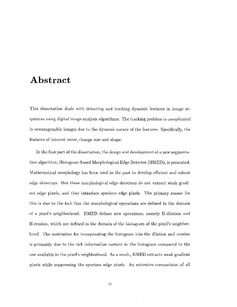
Abstract

This dissertation deals with detecting and tracking dynamic features in image se­

quences using digital image analysis algorithms. The tracking problem is complicated

in oceanographic images due to the dynamic nature of the features. Specifically, the

features of interest move, change size and shape.

In the first part of the dissertation, the design and development of a new segmenta­

tion algorithm , Histogram-based Morphological Edge Detector (HMED), is presented.

M athem atical morphology has been used in the past to develop efficient and robust

edge detectors. But these morphological edge detectors do not extract weak gradi­

ent edge pixels, and they introduce spurious edge pixels. The prim ary reason for

this is due to the fact tha t the morphological operations are defined in the domain

of a pixel’s neighborhood. HMED defines new operations, namely Il-dilation and

Il-erosion, which are defined in the domain of the histogram of the pixel’s neighbor­

hood. The m otivation for incorporating the histogram into the dilation and erosion

is prim arily due to the rich information content in the histogram compared to the

one available in the pixel’s neighborhood. As a result, HMED extracts weak gradient

pixels while suppressing the spurious edge pixels. An extensive comparision of all

morphological edge detectors in the context of oceanographic digital images is also

presented.

In the second part of the dissertation, a new augmented region and edge segmenta­

tion technique for the interpretation of oceanographic features present in the AVHRR

image is presented. The augmented technique uses a topography-based m ethod tha t

extracts topolographical labels such as concave, convex and flat pixels from the im­

age. In this technique, first a bicubic polynomial is fitted to a pixel and its neighbor­

hood, and topolographical label is assigned based on the first and second directional

derivatives of the polynomial surface. Second, these labeled pixels are grouped and

assembled into edges and regions. The augmented technique blends the edge and

region information on a proximity based criterion to detect the features. A num ­

ber of experim ental results are also provided to show the significant improvement in

tracking the features using the augmented technique over other previously designed

techniques.

Chapter 1

Introduction

Remote sensing systems are some of the most prolific sources of digital da ta in the

field of image analysis and understanding. Remote sensing and aerial imagery have

wide applications in geological and soil mapping, land use, land cover, agriculture,

oceanography, water resources planning and in other areas. In most of these applica­

tions, sensors mounted either on satellites or in low flying aircraft provide the digital

da ta (usually imagery) of the scene under study. The problem domain to which these

digital images are applied has correspondingly increased in scope and magnitude.

Image analysis techniques have been used extensively for autom ated in terpreta­

tion of digital imagery. However, current image analysis techniques rely on human

interpretation of the satellite imagery. Human interpretation is obviously varied in

its level of expertise and is highly labor-intensive. W ith the proliferation of digital

and satellite data and the increasing cost of manual interpretation, its becomes highly

desirable, for certain applications, to move toward a capability for autom ated inter-

1

preiation. Digital analysis provides capabilities for making faster and much more

sophisticated interpretation than is possible with the manual approach. Researchers

have shown tha t it is both feasible and com putationally practicable to develop au­

tom ated vision systems to perform on a machine tha t task which the hum an vision

system appears to perform effortlessly [12, 31, 30]. However, most of the vision system

outperlorm ed the human vision systems in numerical com putations, but not in the

interpretation ol the images for reasons due to lack of efficient image processing algo­

rithm s - tha t works on all image settings - and knowledge representation tools. Thus

there is a continuing need for efficient machine implemented analysis of IR da ta using

digital image processing and artificial intelligence techniques. We discuss issues re­

lated to the development of an vision system to segment and interpret oceanographic

features present in Infrared (digital) images in succeeding sections. The feratures

in the oceanographic image change size, position and shape with tim e as explained

below.

1.1 P ro b lem D o m a in

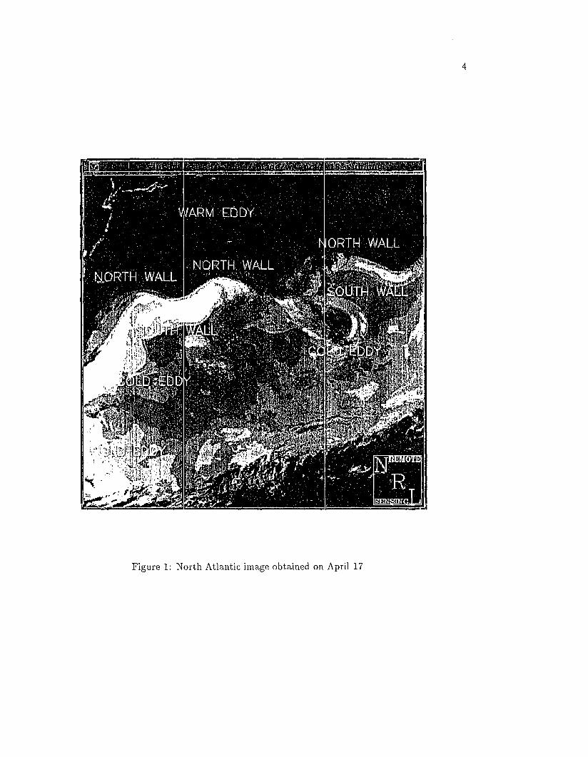
Figure 1 is an Infrared (IR) image of the ocean obtained from the Advanced Very

High Resolution Radiometer (AVIIRR) abroad the NOAA-7 satellite. Such images

are widely used for the study of ocean dynamics. In this image dark shades represent

warmer tem peratures and light shades represent colder tem peratures. This image is

unusually free of clouds and noise caused by atmospheric humidity. The Gulf Stream,

cold eddies, and warm eddies (normally circulating at the north of the Gulf Stream)

are examples of ’’mcsoscale” ocean features with dimensions of the order of 50-300

km.

The Gulf Stream is warmer than the Surgasso sea to its south, and much warmer

than the waters to its north. Thus, its boundaries are easily detectable as edges

produced by the tem perature gradients in satellite IR images [54]. Sometimes clouds

obscure oceanographic features, making their detection difficult. The movement of

these features compounds the problems associated with the detection. For instance,

the Gulf Stream drifts drastically while meandering. Sometimes these meanders lead

to the ’’b irth” of a the Gulf Stream ring, which is a special type of eddy tha t forms

from a cut-off Gulf Stream meander [7, 43, 50]. When the Gulf Stream closes on

itself, surrounding a mass of cold water at its southern boundary, a counterclockwise-

rotating cold ring forms. Similarly, when the Gulf Stream surrounds a mass of warm

water at its northern boundary, a clockwise-rotating warm ring originates.

Cold eddies are typically 150-300 km in diam eter, while warm rings have diameters

of around 100 km [27]. A warm eddy moves generally southwest at 3-8 cm /sec, with

a mean lifetime of about half a year, and ’’dies” by coalescing with the Gulf Stream

[35, 43]. A cold ring drifts southwestward at 5-10 cm /sec while not interacting with

the Gulf Stream , with a mean lifetime of 1.2-1.5 years, and ultim ately coalesces with

the Gulf Stream [43, 46]. Since satellite IR images of the ocean often depict the

mesoscale features clearly, Advanced Very High Resolution Radiam eter (AVIIRR)

imagery is used extensively to study them. The study of the oceanographic features

provides useful information on ocean dynamics and oil spills, and saves millions of

dollars by facilitating navigation through the features. However, autom ated detection

NORTH. WALLNORTH WALL

Figure 1: North Atlantic image obtained on April 17

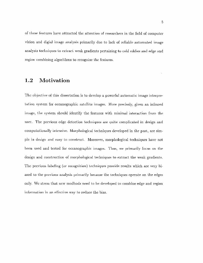
of these features have a ttracted the attention of researchers in the field of computer

vision and cligial image analysis primarily due to lack of reliable autom ated image

analysis techniques to extract weak gradients pertaining to cold eddies and edge and

region combining algorithms to recognize the features.

1.2 M o tiv a tio n

The objective of this dissertation is to develop a powerful autom atic image interpre­

ta tion system for oceanographic satellite images. More precisely, given an infrared

image, the system should identify the features with minimal interaction from the

user. The previous edge detection techniques are quite complicated in design and

com putationally intensive. Morphological techniques developed in the past, are sim­

ple in design and easy to construct. Moreover, morphological techniques have not

been used and tested for oceanographic images. Thus, we prim arily focus 011 the

design and construction of morphological techniques to extract the weak gradients.

The previous labeling (or recognition) techniques provide results which are very bi­

ased to the previous analysis prim arily because the techniques operate on the edges

only. We stress tha t new medhods need to be developed to combine edge and region

inform ation in an effective way to reduce the bias.

1.3 R esea rch C o n tr ib u tio n s

6

The first, part of the dissertation envisages the shortcomings of the traditional mor­

phological operators (explained in chapter 2) in the context of edge detection. We de­

signed and implemented a new algorithm H istogram -B ased M orp h olog ica l E dge

D e te c to r tha t overcomes the shortcomings. The new algorithm bridges two edge de­

tection theories: edge detection by histogram and edge detection by m athem atical

gray scale morphology. We also show tha t the traditional morphological edge detec­

tors are only a class of histogram-based morphological edge detectors. Our techriic|ue

is applied to oceanographic satellite data and the results are compared with two other

well known algorithms.

In the second part of the dissertation, a T opography-B ased F eature L abeling

technique is presented. In this method, a general com putational framework is de­

signed l,o address the problem of labeling oceanographic images. The essential ideas

stem lrom fitting a bicubic polynomial to each pixel’s neighborhood and assigning

topological labels based on the first and second directional derivatives of the polyno­

mial surface. The relationship between the oceanographic features in infrared satellite

imagery and the topographic structures is also designed. Algorithms are developed

tha t dem onstrate ability to locate and identify the North and South Walls of the Gulf

Stream and to find approxim ate centers of Warm and Cold eddies. Experim ental re­

sults on detecting these oceanographic features are also provided.

7

1.4 O rgan iza tion o f th e D isse r ta tio n

A concise overview of digital image processing and the edge detection techniques in

the context of oceanographic images is given in succeeding subsections. In chapter 2

we bring the preliminary concepts and previous morphological techniques. In chapter

3 we design and implement the histogram-based morphological techniques, including

the parallel and distributed implementation. The feature labeling techniques in the

context of oceanographic data is discussed in chapter 4. In chapter 5 the Topography-

based feature labeling technique is designed and implemented. We conclude with the

future goals in chapter 6.

1.5 D ig ita l Im age P r o c e ss in g - In tr o d u ctio n

Digit al image processing is basically concerned with com puter processing of pictures

(or images) tha t have been converted into a numeric form. It is a process of ex tract­

ing, characterizing and interpreting information from images of a three-dimensional

world. This process is commonly divided into six principal areas: (1) Sensing, (2)

Preprocessing (3) Segmentation (4) Description (5) Recognition (6) Interpretation.

Sensing is a process tha t yields a visual image. Preprocessing deals with techniques

such as noise reduction and enhancement of details. Segmentation is a process tha t

partions an image into objects of interest. Description deals with the com putation

of features suitable for differentiating one type of object from another. Recognition

is the process tha t identifies these objects (e.g., wrench, bolt, nut, wheel). Finally,

interpretation assigns meaning to an ensemble of recognized objects. Sometimes,

these subdivisions are grouped under three categories: Low-level, Medium-level and

High-level vision. For instance, sensing and preprocessing are grouped under low-level

vision, segmentation, description and recognition are grouped under medium-level vi­

sion, and interpretation is grouped under high-level vision. Most of the vision systems

are implemented based on these three levels of vision. In general, the purpose of dig­

ital image processing is to enhance or improve the image in some way, or to extract

information from it.

An image is divided into small regions called picture elements, or pixels for short.

The most common subdivision scheme is the rectangular sampling grid. The image

is divided into horizontal lines made up of adjacent pixels. At each pixel location,

the image brightness is sampled and quantized. This step generates an integer at

each pixel representing the brightness or darkness of the image at th a t point. When

this has been done for all pixels, the image is represented by a rectangular array of

integers. Each pixel has a location or address (line or row number and sample or

column number) and an integer value called the gray level. This array of digital data

is now a candidate for com puter processing.

Digital image processing starts with one image and produces a modified version of

tha t image. It is a process tha t takes an image into an image. Digital Image analysis

is taken to mean a process th a t takes a digital image into something other than a

digital image, such as a set of measurement data.

Digitizing is the process of converting an image from its original form into digital

form. The term conversion is used in a nondestructive sense because the original

image is not destroyed but is used to guide the generation of a digital image.

9

Scanning is the selective addressing of specific locations within the domain of an

image. Each of the small sub-regions addressed in the scanning process is called a

picture element, or pixel for short. The term scanning is loosely taken as an equivalent

to the term digitizing. The rectangular grid scanning pattern is known as a raster.

The notion of contrast refers to the am plitude of gray level variations within an

image. Noise is broadly defined as an additive (or multiplicative) contam ination of

an image. The sampling density of a digital image is the number of sample points

per unit measure in the domain. Gray Scale resolution is the number of gray levels

per unit measure of image amplitude. Magnification refers to the size of relationship

between an image and object or image it represents.

The operations tha t can be performed on digital images fall into several classes.

An operation is a global operation if it is applied equally throughout the entire digital

image. A point operation is one in which the output pixel value depends only on the

value of the corresponding input pixel. Point operations are sometimes called contrast

m anipulation or stretching. A local operation is one in which the output pixel value

depends on the pixel values in a neighborhood of the corresponding input point.

In an image of a scene there are a variety of sources of low-level information

available which can be used to form an initial description of the structure of the

image. The extraction of this description, in term s of significant image tokens, is an

im portant precursor to the construction of a more abstract description at the semantic

level. It is unlikely tha t any single descriptive process will produce a description tha t

is adequate for an unambiguous interpretation of the image.

10

Many segmentation algorithms or low-level processes use some form of smoothing

operation as a preprocessing stage. Image clata are complicated by errors of approxi­

mation due to the discrete nature of the representation, noise intrinsic to the sensors,

and variations in the scene itself. Most simple smoothing operators do not remove

noise w ithout destroying some of the fine structure in the underlying image.

One of the simplest and most useful tools in digital image processing is the gray

level histogram . This function summarizes the gray content of an image. The gray

level histogram is a function showing the number of pixels in the image tha t have a

particular gray value. The global histogram for many images tend to be gaussian in

shape, and the area under the curve is the total number of pixels in the image. It

is noted here, when an image is condensed into a histogram, all spatial information

is lost. The histogram specifies the number of pixels having a particular gray level

but gives no hint as to where those pixels are located within the image. Thus the

histogram is unique for any particular image, but the reverse is not true.

The global histogram may not be very useful for extracting vital cues from the

image because the global information will not accurately reflect local image events

tha t do not involve large numbers of pixels. Much of the focus of the algorithms will

be to organize the segmentation process around local histograms from local windows

and then have a postprocessing stage merge regions tha t have been arbitrarily split

along the artificial window boundaries. Histogram is useful for enhancing the image,

changing the contrast of the image, thresholding the image.

T h resh o ld in g is process of segmenting objects of interest from the background

of the image based on the gray value of the pixels in the image. Suppose we have

11

a light object on a dark background. One obvious way to segment the object is to

choose a threshold (or gray) value T, such tha t a pixel whose gray value is less than

T can be background pixel and if it greater than T, it is a pixel belonging to the

object. Histogram is useful for thresholding operation. Multilevel thresholding is also

useful if the image has one or more different objects in the image. In other words,

we choose different values T l, T2, etc, such tha t pixel value greater than T2 belong

to one object. , pixel value less than T l belong to a background, pixel value greater

than T l and less than T2 may belong to another object.

A classical problem in image processing is the detection of sudden changes in gray

values from one pixel to another adjacent pixel. Such changes usually indicate a

boundary, i.e., an edge, between two distinctly different objects in the image. If the

difference in gray values between two adjacent pixels vary considerably, then the pixels

are named as edge pixels. This method of detecting edges is called edge d e tec tio n

by thresholding. The detection of these edges is very im portant for analyizing the

objects in the image. Moreover, this operation reduces the amount of data present in

the image. In other words, previously, we have huge amount of pixels in the original

image. After this operation, we have only pixels tha t belong to the objects of interest.

Most of the autom ated vision systems tha t have been developed for the image

interpretation partitions the entire process into manageable pipelined subtasks with

or w ithout feedback. As mentioned earlier, a traditional conceptual classification

divides an image analysis task into three basic modules: low, medium and high level

analysis. The purpose of this type of classification of the vision system is to decompose

the overall complexity of the problem into manageable portions. However, there is

12

no fixed dividing lines in the sequence of operations from image sensing through

preprocessing, boundary detection, region growing and interpretation.

The low level analysis tasks preprocess and segment the image, and extract statis­

tical values, texture, tone from the image without using any domain-specific knowl­

edge. The process of partitioning an image into primitives is defined as segmentation

[53]. The choice of one segmentation algorithm over another is dictated mostly by

the characteristics of the problem being considered. Segmentation has become a pre­

requite for the description of an image. The main idea behind segmentation step is not

only to reduce the massive amount of pixel data but also to extract local param eters

to interpret the image.

For example, each pixel has three param eters associated with it: x and y coordi­

nates, and an intensity value typically in the range 0-255. A pixel does not have any

other information about the objects in the image. It is extremely difficult to interpret

a 512 x 512 image, using only the information provided by the pixels; they provide

a great deal of information, but not in a useful form. It is necessary to reduce the

quantity of data w ithout losing any structural information contained in the image.

In transforming a raw image to a more reduced data format, a number of param eters

are extracted namely, statistical data, texture, tonal values and many others.

This process of extracting param eters is widely known as low-level image analy­

sis. In the last two decades, a number of low-level image processing algorithms for

segmenting a raw image have been developed. However, none of the image process­

ing techniques work in all image settings. Some techniques are sensitive - to noise

in the image, to the light condition under which the objects have been sensed, to

threshold param eters and to other parameters. The common problem with the tech­

niques is tha t some im portant features are not extracted and/or erroneous features

are detected.

Sometimes image processing techniques require some kind of domain-specific knowl­

edge for them to provide reliable results. Techniques of this type make up the inter­

mediate level. Region growing, shape analysis, probabilistic relaxation, m ultispectral

classification are examples of medium-level segmentation algorithms. The am ount of

knowledge incorporated in these techniques depends on the objects in the scene and

effectiveness of the techniques.

The high level tasks unambiguously apply meaningful labels to objects in the

images using shape, size, position and other information provided by the medium

level modules. All domain-specific knowledge available is used to label the images.

For instance, tone, texture, interrelationship between the features, and the seasonal

variations and the dynamic nature of the feature, if any, are used in the high level

module. A number of high level vision techniques have been reported in recent years

to describe and interpret the output of the lower-level modules. The representation,

use, and the acquisition of the knowledge constitutes the heart of any autom ated

vision systems. W ith the fusion of Artificial Intelligence techniques in the com puter

vision, knowledge representation led to a shift from the procedural to declarative

forms. Production rules, semantic nets, frames, blackboard architectures are some

of the well known and widely used forms of knowledge representation and inference

mechanisms of high-level vision techniques.

14

HM ED

Expert System

TopographyLabelingIR image

PreviousAnalysisRelaxation

Labeling

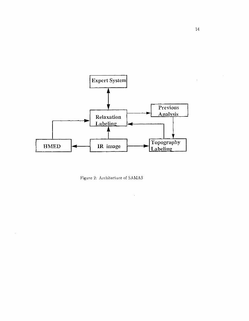
Figure 2: Architecture of SAMAS

15

Traditionally, to improve the effectiveness of the three modules, a feedback from

the medium-level to the low-level module and from the high-level to either medium-

level or low-level or both is provided. Tenenbaum and Barrow [52] dem onstrated

the effectiveness of feedback of domain specific knowledge from the medium to the

low-level (the concept of interpretation guided segmentation). Nagao [33] suggests

tha t the segmentation process should be a trial-and-error recursion between the data-

driven segmentation and the goal-directed recognition in order to reach a better seg­

m entation of the scene. They also proposed a compact and intim ate intergration of

segmentation with interpretation, in which an initial segmentation using a standard

image-processing procedure is approxim ately interpreted and repeatedly modified, for

in terpretation to become complete and consistent. Hanon and Riseman [12] imple­

m ented a vision system for natural scenes in which feedback paths were provided to

integrate semantics of the domain into segmentation processes, with the notion tha t

segmentation errors will be reduced with the help of domain specific knowledge. We

discuss a vision system for interpretation of oceanographic data.

1.6 E d g e D e te c t io n in O cean ograp h ic Im a g es

The Naval Research Laboratory began development of the Semi-Automated Mesoscale

Analysis System (SAMAS), a comprehensive set of algorithms to handle the auto­

m ated analysis problem, from low-level segmentation through intermediate-level fea­

ture formation and higher-level Artificial Intelligence modules tha t estim ate positions

of previously detected features when cloud cover obscures direct observation in the

current image set [26].

16

The current version of SAMAS (Figure 2) groups various modules into these three

categories. A cloud detection algorithm processes the therm al infrared image of the

ocean to classify all pixels either as cloud pixels or non-cloud pixels [51]. Considering

only non-cloud pixels, the system uses the cluster shade texture measure as the low-

level operation and detection of zero crossings in cluster shade as the medium-level

operation, leading to a set of edge primitives [16]. SAMAS uses two-step nonlinear

relaxation [20] to label edge primitives [22]. In the first, relaxation labeling step, a

priori probability values of the edge pixels are computed using a priori knowledge of

the approxim ate sizes and positions of the features, based on a previous analysis (typ­

ically from one week earlier). In the second step, these probability values are updated

using com patibility coefficients in an iterative fashion, until the values stabilize. The

relaxation labeling techniciue reduces uncertainty in the assignment of labels to edge

pixels [22], We also developed a topographic-based feature labeling module tha t uses

the surface topology of a pixel and its neighborhood [24, 25].

First we discuss the features of the edge detection algorithm proposed by Ilolyer

and Peckinpaugh, the popular derivative-based edge operators, viz Sobel’s operator,

are shown to be too sensitive to edge fine-structure and to weak gradients to be

useful in this application. The edge algorithm proposed by Holyer and Peckinpaugh

is based on the cluster shade texture measure, which is derived from the gray level

co-occurrence (GLC) m atrix. The authors suggest tha t the edge detection technique

can be used effectively in the autom ated detection of mesoscale features. The (*, j ) th

element of the GLC m atrix , P ( i , j \ Ax , Ay ) , is the relative frequency with which

two image elements, separated by distance ( Ax, Ay) , occur in the image, one with

intensity level i and the other with intensity level j. The elements of the GLC m atrix

could be combined in many different ways to give a single numerical value th a t would

be a measure of the edges present in the image. Ilolyer and Peckinpaugh use a cluster

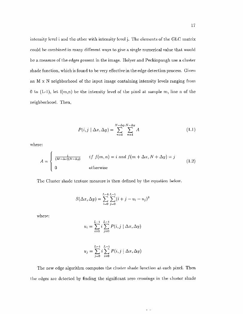
shade function, which is found to be very effective in the edge detection process. Given

an M x N neighborhood of the input image containing intensity levels ranging from

0 to (L -l), let f(m,n) be the intensity level of the pixel at sample m, line n of the

neighborhood. Then,

N —A y N —A y

P ( i , j \ A x , A y ) = E E A (1-1)n = l n = l

where:

i f f ( m , n) = i and f { m + Ax , N -f Ay) = j/I ( M - A . r ) ( N - A . , ) - - ^ ^

0 otherwise

The Cluster shade texture measure is then defined by the equation below.

S{ Ax , Ay ) = E E ( i + J ~ ui ~ ui ) 3z = 0 .7=0

where:L - 1 L - l

=E iE P( j I A‘t ’ a )i = 0 j = 0

= E i E I A x , A y )j—0 i—0

The new edge algorithm computes the cluster shade function at each pixel. Then

the edges are detected by finding the significant zero crossings in the cluster shade

18

image. Note tha t (1) the cluster shade can assume either positive or negative values,

(2) the values are the largest in the vicinity of the north wall of the Gulf Stream , (3)

values are negative on one side of the wall and positive on the other side, and (4) the

transition point from large positive to large negative values coincides with the exact

location of the edge of the Gulf Stream. These observations suggest tha t one could

detect edges by finding significant zero-crossings in the cluster shade image.

Significant zero-crossings in the cluster shade image is determined as follows. An

initial threshold is selected. Then, for each 3 x 3 pixel neighborhood in the cluster

shade image, the absolute value of center pixel is tested with the threshold. If it is less

than the threshold, a value ”0” assigned in the binary output image. If the absolute

value of the center pixel exceeds the threshold, then a test of the neighboring pixels

is performed. If the absolute value of any of the eight neighboring pixels also exceeds

the threshold, but is opposite in sign from the center pixel, a value ” 1” is assigned in

the binary image indicating the presence of an edge pixel. Because edges are detected

by finding zero crossings, precisely positioned lines result, even if the GLC m atrix

is calculated using a larger window. So, the desired edge detection characteristic of

retaining sharp edges while eliminating edge detail is achieved by the new algorithm.

It is known tha t using large windows in derivative-based edge detector algorithms

results in poor smoothing. This problem is circumvented in the new algorithm. As

an input to our feature labeling algorithm, we used the output image generated by

cluster shade algorithm, with a window size of 16x16 pixels and zero crossing threshold

of 50. The edge magnitudes obtained from this new edge detector algorithm are used

as an input to the feature labeling algorithm. In particular, the edge magnitudes are

19

'REMOTE]

Figure 3: Edges extracted from Figure 1 using CSED

20

used to evaluate the a priori probability values. Figure 3 shows the output of the

edge detector on image 1 (Figure 1 ).

Cayula and Cornillon [4] have developed an edge-detection algorithm for oceano­

graphic satellite images. Their algorithm operates at three levels: picture level, win­

dow level, and local/pixel level. At the picture level, most obvious clouds are identified

and tagged so tha t they do not participate at the lower levels. The cloud-finding pro­

cedure is based on tem perature and shape. At the window level, the tem perature

distribution in each window is analyzed to determine the statistical relevance of each

possible fronts, using unsupervised learning techniques. Finally, local edge operators

are used to complete the contours found by the region-based algorithm. Since the

local operations are used along with the window-based algorithm, the qualities of

scale invariance and adaptivity associated with the region-based approach are not

lost. Cayula [3] compare the edge-detection algorithm described above. The main

difference is tha t the algorithm given by Ilolyer and Peckinpaugh operates at the local

level only, while tha t by Cayula and Cornillon is a multilevel algorithm. Refer to [3]

for the details on the results of the comparison.

Chapter 2

Morphological Edge Detectors

M athem atical morphology based on geometric shape, is used in biomedical image

processing, robot vision systems, and low-level vision problems for its conceptual

simplicity. Many techniques in com puter vision use m athem atical morphology as a

tool for the extraction of features and recognition of objects. M atheron [29] introduced

the application of m athem atical morphology for analyzing the geometric structure of

metallic and geologic samples. Serra [47] applied m athem atical morphology for image

analysis. Haralick [15] presented a review of m athem atical morphology applied to

image analysis.

Pelag and Rosenfeld [38] use gray scale morphology to generalize the medial axis

transform to gray scale imaging. Pelag et al [37] measure changes in texture properties

as a function of resolution using gray scale morphology. W erman and Pelag [56] use

gray scale morphology for texture feature extraction. We will study the use of gray

scale morphology and texture information for edge detection in oceanographic images.

21

Recently, m athem atical morphology has been applied for the extraction of edges.

Most of the tem plate based edge detectors are known to perform satisfactorily under

high signal to noise ratio, but degrade significantly when noise is introduced into the

system. Some of the tem plate based edge detectors are the Prew itt operators and the

Kirsh operator. A number of edge detectors fit a polynomial function on the image

data. Then, the first and second directional derivatives are com puted, from which

the edges are extracted. M athem atical morphology based edge detectors have been

shown to out-perform most spatial and differentiation based edge detectors [45]. Mor­

phological edge detectors are local neighborhood nonlinear operators. Morphological

techniques tend to simplify image data while preserving the shape characteristics

and elim inating irrelevancies. These algorithms often generate useful and surpris­

ing results. We briefly present preliminary concepts of m athem atical morphology.

M atheron [29] gives a detailed discussion of m athem atical morphology.

2.1 P re lim in a r y C o n cep ts

An image is a set of pixels in a rectangular array (mesh). f(i, j ) is a pixel at coordi­

nate (i, j ) in the image /. A structuring element is analogous to the kernel/tem plate of

a convolution operation, and it is associated with a pre-designed shape. A structuring

element may have any shape. Morphologic operators can be visualized as working

with two images, the original image and the structuring element. The structuring

element is used as a tool to m anipulate the image using various operations namely

dilation, erosion, opening, closing. The dilation of a binary image / by a

structuring element S is defined as

/ © S = { ct —(- b | a £ / A i G 5}

The erosion of a binary image / by a structuring element S is defined as

/ © S = { a — b | a E f A 6 £ 5}

The n di lation” d of a gray-scale image / by a structuring element S is defined as

d. (i , j ) = M A X ( f ( i + x j + y) © S{x, y))

where x and y are the coordinates of a cell in S whose center cell is the origin, and

(i+x, j+ y ) is in the domain o f / . Similarly, ’’erosion” of a gray-scale im a g e / by a

structuring element S is defined as

e( i , j ) = M I N ( f ( i + x , j + y) Q S { x , y))

The closing operation is a dilation followed by an erosion, and similarly opening is an

erosion followed by a dilation. Thus, closing is defined as

c{ i , j ) = M I N ( d ( i + x , j + y) 0 S( x , y ) )

where d is the dilated image of original image f . Opening is defined as

o{ i , j ) = M A X ( e ( i + x , j + y) © S( x, y))

where e is the eroded image of original image /. A sequence of these gray scale

morphological operations on an image often produces useful results. For instance, a

simple morphological edge detector is the dilation residual edge image, defined as

24

DR (i , j ) = d (i , j ) - f (i , j)

Similarly, t,he erosion residual edge detector is given by

ER (i , j ) = f (i , j ) - e (i , j)

Even though these edge detectors are simple and robust, they are not reliable for

extremely noisy images, and introduce spurious edges.

2.2 B lu r -M in im iza tio n M o rp h o lo g ica l O p era tor

Lee et a,I [17] designed a Blur-Minimization Morphological (BMM) operator for edge

detection. The BMM operator blurs the original image by averaging the pixel values

spanned by the structuring element. Dilated and eroded images are generated from

the blurred image. Dilation residual and eroded residual images are created using

these images. The edge strength at coordinate (i, j) is given by the minimum of the

dilation residual and erosion residual. Symbolically we write

BMM(i, j) = MIN ( /„ ( i, j) - e(i, j), d(i, j) - f a{i, j))

where f a = llZh+pi+sd jg ^ jurreci ;m age, N is the number of cells in the structuring

element, and (i+x, j+ y ) is defined in the domain of the image. In spite of being

conceptually simple and com putationally efficient, the BMM edge detector has been

proven to perform better than the spatial and differential based edge detectors.

2 .3 A lp h a -T rim m ed M orp h o log ica l O p erator

Feehs and Arce [42] showed the im portance of blurring the original image for mor­

phological edge detection. They introduced a Alpha-Trimmed, multidimensional Mor­

phological (ATM) edge detector tha t incorporates the opening and closing operations.

They also proved statistically th a t ATM performs better than BMM. Let us consider

the ATM edge detector for 2 -dimensional images with a structuring element of size

y^k~a j ,n x n. The original image is initially blurred by f a = where k = n2 is the

number of pixels in the original image spanned by the structuring image, /,■ is the i lh

smallest valued pixel in the sorted sequence of pixels in / spanned by the structuring

elem ent, and a is the trim m ing factor. If a is 0, we consider all pixels spanned by the

structuring element for blurring. If a = i, we consider all sorted pixels greater than

/,: and less than spanned by the structuring element. The edge strength at (i, j)

com puted by the ATM edge detector is

ATM(i, j) = MIN ( ( o (i,j) - e (i, j ) ) , d (i, j ) - c (i,j) )

in which the erosion and dilation operation are performed on the a trim m ed blurred

image, and the opening and closing operation are performed on the eroded and dilated

images of the a trim m ed blurred image.

The ATM edge detector, like the BMM edge detector, is unable to extract the

weak gradients associated with certain mesoscale features [25]. This could be possibly

because the definition of gray-scale dilation and erosion considers only the maximum

and the minimum intensity pixels in a given neighborhood of a pixel. As a result,

the dilation and erosion residual values are not sufficient for these edge detectors to

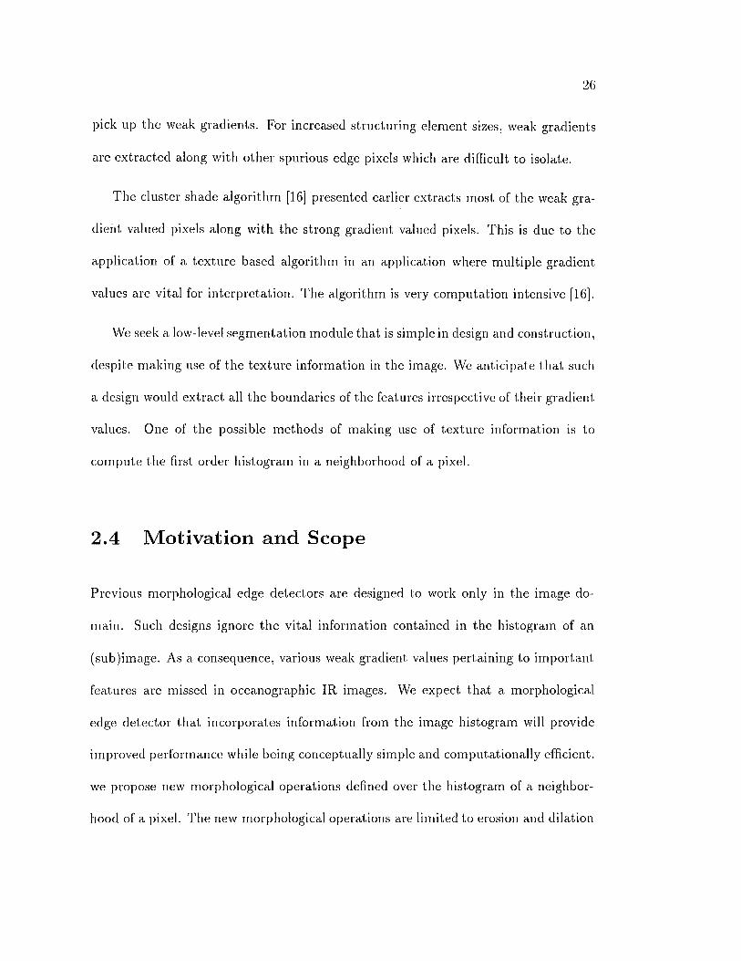
pick up the weak gradients. For increased structuring element sizes, weak gradients

are extracted along with other spurious edge pixels which are difficult to isolate.

The cluster shade algorithm [16] presented earlier extracts most of the weak gra­

dient valued pixels along with the strong gradient valued pixels. This is due to the

application of a texture based algorithm in an application where multiple gradient

values are vital for interpretation. The algorithm is very com putation intensive [16].

We seek a low-level segmentation module tha t is simple in design and construction,

despite making use of the texture information in the image. We anticipate tha t such

a design would extract all the boundaries of the features irrespective of their gradient

values. One of the possible methods of making use of texture information is to

compute the first order histogram in a neighborhood of a pixel.

2 .4 M o tiv a tio n an d S cop e

Previous morphological edge detectors are designed to work only in the image do­

main. Such designs ignore the vital information contained in the histogram of an

(sub)image. As a consequence, various weak gradient values pertaining to im portant

features are missed in oceanographic IR images. We expect tha t a morphological

edge detector tha t incorporates information from the image histogram will provide

improved performance while being conceptually simple and com putationally efficient,

we propose new morphological operations defined over the histogram of a neighbor­

hood of a pixel. The new morphological operations are limited to erosion and dilation

27

only, and the morphological basis of these new operations is explained in the context

of oceanographic images only [23].

Chapter 3

Histogram-Based Morphological Edge D etector

The histogram is a popular tool used in image processing and image analysis. It

is used for edge detection, thresholding, texture feature extraction and other related

problems. Let H be the histogram of an image or sub-image, let go,gi, •■■,gi-1 be the

gray levels for which the histogram is defined, and h(g0), h(gi ) , ..., h(gi-i) be the count

values for those gray levels. Previously, researchers have designed image segmenta­

tion methods from the histogram using either global or local thresholding concepts.

For instance, when a light object is present in dark background, the histogram may

have twin peaks occurring at the intensities corresponding to the intensities of the

object and background. A suitable threshold between the two peaks is selected to

segment the object from the background [49]. When multiple objects are present in

the background, a global histogram is of little use. However, a local histogram in

the neighborhood of a pixel would exhibit twin peaks from which an object can be

28

29

the neighborhood of a pixel would exhibit twin peaks from which an object can be

segmented from the background [45].

It is noted tha t the gray scale dilation and erosion are the maximum and minimum

of the image pixels spanned by the structuring element, respectively. The definitions

of gray scale morphology, in fact, make use of the histogram indirectly. This is ex­

plained using a structuring element S of height 0 in the following way: gray scale

dilation over the histogram is the maximum of go-, fji, fji, ■■■gi-1 for which h^gi) 7 0 .

Similarly, the gray scale erosion is the minimum of </0, </i, gi, . ..gi-1 for which h^gi) 7 0.

The average of the image pixels is computed from the histogram. It is also noted tha t

the BMM and ATM edge detectors extract edges using the gray scale dilation and

erosion operations. But, these definitions consider only the maximum and minimum

of the image pixel intensities in a given neighborhood. Thus, we infer tha t there is

a clear distinction in theories between the histogram based edge detectors and m or­

phology based edge detectors. The essential ideas in the former methods stem from

the fact th a t the histogram taken near the boundaries exhibits twin peaks, while

the la tter methods mark a pixel as an edge pixel depending on the maximum and

minimum intensity values of the pixels near the boundaries. We anticipate th a t m or­

phological edge detectors tha t use the histogram in an effective way would reduce the

gap between these two edge detection theories. In doing so, we will develop exten­

sions to the definitions of morphological operations in the domain of the histogram,

but not in the domain of the image. We anticipate tha t such extensions provide us

new directions in the notion of morphology-based edge detectors, particularly in the

context of oceanographic images.

30

Let a histogram II defined over gray levels g0, g \ , g i - i , be com puted using the

image pixels spanned by the structuring element S centered at the coordinates (x,

y). g0 and are the intensity of black and white pixels, resp. Call the height of

the histogram at these gray levels h(g0), h( gi ) , ..., h(gi-i). Let the intensity of the

pixel (at coordinates (x, y)) - where the histogram is computed - be gi. We define

histogrammic dilation h-ililation at a pixel (x, y) as

4 ( x , y) = {gj | = ma.x[h(gi),h(gi+2) , . . . . , l i {gi-i) ] and (i < j < 1- 1 )}

Similarly, we define the histogrammic erosion h-crosion as

e*(x, y) = {gj | h(gj) = m a x [% 0), and ( 0 < j < i)}

It is noted tha t both the r//, and e/, are defined in term s of peaks of the histogram

on either side of the gray level intensity </,- of the pixel. By defining these operations in

this fashion, we make a noticeable deviation from the traditional dilation and erosion

operations.

The value of e/t is the gray level intensity ge at which the histogram height is the

maximum of all heights com puted at gray level intensities lower than the (average)

gray level intensity of the pixel. The value of dh is the intensity gj at which the

histogram height is the m aximum of all histogram heights computed at intensities

greater than the (average) intensity of the pixel. In case an unique intensity ge (gj)

is not found, gc (gd) th a t is closer to g, is selected.

One of the motivations for using h-dilation and h-erosion is as follows. Figure

1 is unusually free of clouds. Even though many cloud detection algorithms are

31

available, none of them detect all cloud pixels [51]. Therefore some cloud pixels will

be present in the input image. We recall tha t the traditional dilation and erosion

definitions consider only the extrem e values in the neighborhood of a pixel. If a

cloud pixel is one of the extrem e values, then an edge detector based on traditional

m athem atical morphology will extract spurious edge pixels. We anticipate a reduction

in the extraction of spurious edge pixels when we use the h-dilation and h-erosion

operations.

A careful exam ination of these definitions indicates a strong link between the

histogram based and morphology based edge detectors. For instance, consider a

histogram computed in a neighborhood of a pixel near the boundary having (twin)

peaks with the average intensity falling between the peaks. The histogram based

methods search for the valleys and peaks in the histogram, whereas the morphological

methods (BMM and ATM) search for the extreme intensities tha t have non-zero

histogram heights.

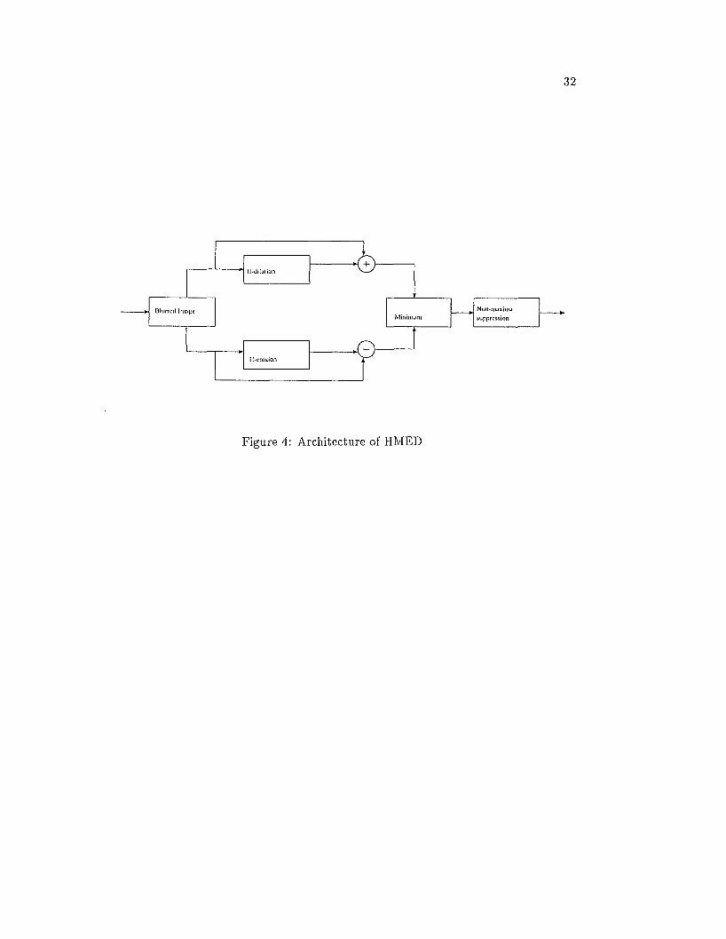
Figure 4 is the new edge detector tha t makes use of the histogrammic dilation and

erosion. The edge strength in the edge image at (x, y) is given by

IIMED(x, y) = min ( /(x, y) - e,,.(x, y), dh(x, y) - ,/(x, y))

where / (x, y) is the average intensity gi at coordinate (x, y).

Thus, the edge m agnitude values in the output image are computed in a similar

fashion to tha t of the BMM and ATM edge detectors. Normally, an edge detector

should generate edge pixels of width two in case of ideal step edges. However, this is

not true for edge detectors tha t take input images which are blurred or smoothed ver-

32

M in im u m

! l - c r o s io n

Figure 4: Architecture of HMED

sions of the original image. The HMED technique, when used with large structuring

elements, produces significant non-zero edge strength of width more tha t one pixels.

This is consistent with the fact tha t HMED blurs the original image. Usually, the

true edge pixels get assigned higher edge strength than their neighbors. Normally,

a suitable threshold is selected to extract the true edge pixels. However, HMED

extracts the true edge pixels using a non-maxima suppression technique.

Thus, we establish a com putational framework tha t adapts the advantages of two

edge detection theories. W ith such a com putational framework, we show tha t HMED

performs better than the BMM and ATM edge detectors.

3.1 H M E D A lg o r ith m

The HMED algorithm given below takes a blurred image as input and produces an

edge strength image in which non-maxima suppression has to be performed. This

procedure uses functions GET-INTENSITY and IIIST(i) tha t return the intensity g

when the coordinates (x, y) of a pixel are given, and the count of pixels with gray

level intensity i, resp. The constant MAXGRAY = 255 is defined.

It is noted tha t a new histogram is not computed from scratch at every pixel’s

neighborhood. The histogram of the adjacent neighborhood (x, y+1) is computed by

using the histogram com puted at pixel (x, y) as described in version 6 in [1 2 ],

The HMED algorithm presented here involves only param eters such as the size of

the structuring element and non-maxima suppression. No strict rules can be stated

in this regard. For the images considered here we present results tha t are produced

34

P R O C E D U R E HMED (blur Amy, diLimg, erdJmg, outJmg, W)

BEGIN

1. for each pixel P(x, y) in the blurred image

BE GIN

2. compute a histogram H of the sub-image ( W x W) centered at (x,y)

3. max = getJntensity (x, y)

4■ For i — max to M A X G R A Y (* dilation operation *)

5. i f ( hist(i) > hist (max) )

6. max = i;

7. diLimg(x, y) = max ;

8. max = get-intensity (x, y)

9. For i = 0 to max (* erosion operation *)

10. i f ( hi.st(i) > hist (max) )

11. max — i;

12. enLimg(x, y) = max ;

13. tempi = blur-img(x,y) - erdJmg (x, y);

If- temp2 = diLimg (x, y) - blurJmg (x, y);

15. outJmg (x, y) = MIN ( tempi , tcmp2);

END

END

,35

with structuring element sizes 15 x 15,17 x 17,19 x 19 and 21 x 21.

There are at least two ways in which we can extract the true edges: com putation

ol zero crossings and suppression of non-maxima.

1. to extract zero-crossings, let us consider line 15 in the algorithm. If tem p i is

minimum, then -tem pi (negative value) is assigned in the edge strength image,

otherwise -ftemp2 (positive value) is assigned. Then a zero-crossing test has

to be performed. The significance of a negative value is tha t the histogram is

skewed to the negative side of the mean value. A positive value indicates tha t

the histogram is skewed to the positive side of the mean value.

2. In case of non-maxima suppression in the edge strength image, we suppress a

pixel as a non-edge pixel if there exists a group of pixels whose value is much

greater than the pixel to be suppressed [24].

3 .2 H a n d lin g o f C lou d C over

The test image in Figure 1 is unusually free of clouds. A typical oceanographic image

contains cloud cover as well as attenuation due to water vapor. Thus the low-level

vision algorithms have to be designed to handle the cloud cover. One simple method

to avoid the cloud pixels is to generate a cloud mask using a technique proposed in

[6 ]. The cloud mask is a binary image tha t contains the values 0 or 1. A value 0

signifies tha t the pixel is part of a cloud and 1 signifies a non-cloud pixel. In this

application, cloud pixels are treated as follows:

1. A pixel in the IR image is considered a candidate edge pixel if and only if the

cloud mask has value 1 a t the same coordinate.

2. For a candidate edge pixel, the histogram is computed by considering only the

non-cloud pixels

3.3 Im p le m e n ta tio n R e su lts

The test data set consists of 12 satellite IR images of the North Atlantic. We present,

results from 3. We processed the images with the BMM and ATM detectors using

structuring elements of sizes 5 x 5, 7 x 7, 9 x 9, 11 x 11, and 13 x 13, while we used

structuring element sizes of 13 x 13, 15 x 15, 17 x 17, 19 x 19, and 21 x 21 with the

HMED detector. The ATM edge detector’s a param eter was 3 in all cases. We do

not, know of any strict rules to govern the choice of the structuring elem ent’s size or

the value of o'.

Figures 5 and 6 all show the results obtained with Figure 1. Figure 5 shows the

results of applying the BMM edge detector with structuring elements of sizes 5 x 5 , 7

x 7, 11 x 11, and 13 x 13. Increasing the structuring elem ent’s size results in finding

more edges. Figure 6 shows the results of applying the ATM detector with structuring

elements of sizes 5 x 5, 9 x 9 , 11 x 11, and 13 x 13. The results are slightly different,

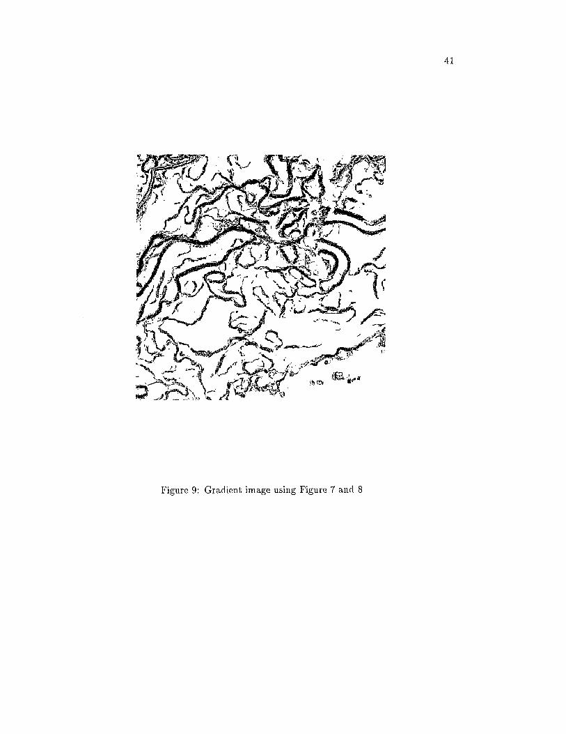
but again increasing the structuring elem ent’s size finds more edges. Figure 7 and

Figure 8 are the h-dilated and h-eroded images of Figure 1. Figure 9 is the gradient

image created by taking the minimum of the residuals (line 15 of the algorithm).

Figure 10 shows the results of applying the IIMED detector with window sizes 13 x

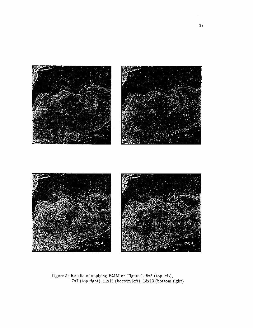
Figure 5: Results of applying BMM on Figure 1, 5x5 (top left),7x7 (top right), 11x11 (bottom left), 13x13 (bottom right)

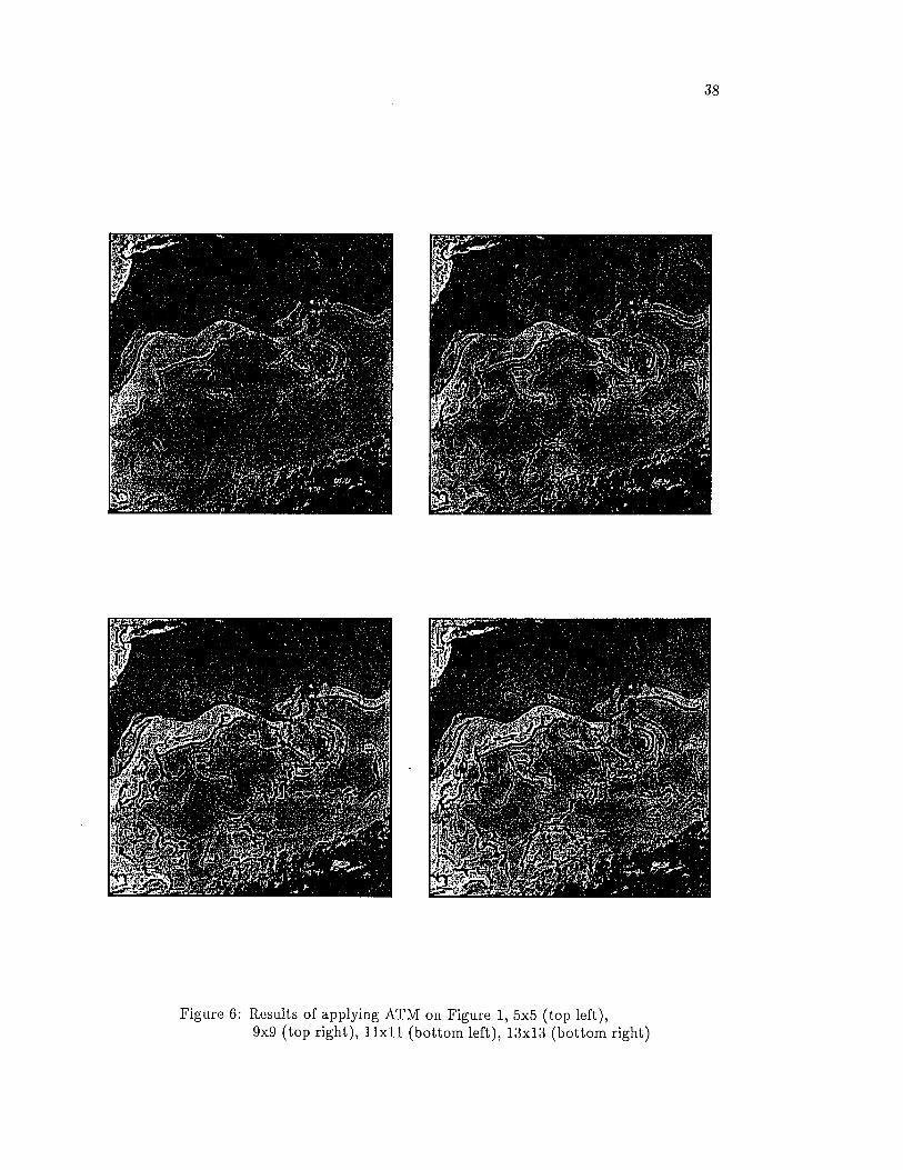
Figure 6 : Results of applying ATM on Figure 1, 5x5 (top left),9x9 (top right), 11x11 (bottom left), 13x13 (bottom right)

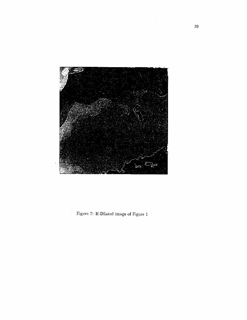
Figure 7: H-Dilated image of Figure 1

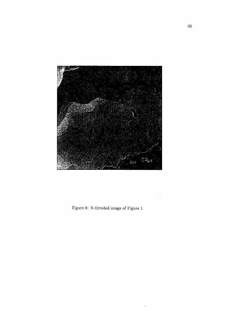
Figure 8 : II-Erroded image of Figure 1

41

Figure 9: Gradient image using Figure 7 and 8

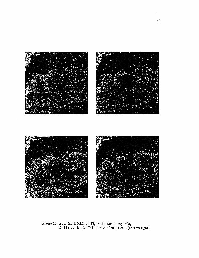
Figure 10: Applying IIMED on Figure 1 - 13x13 (top left),15x15 (top right), 17x17 (bottom left), 19x19 (bottom right)

l&TXrl '

•• - ••■ •

*0v^ /V '^V -U V ^ f'- %i).tj."j> ! 1 ( V * /

' 7, V /sC'\ itr >

* V'/?\- *

' ‘V rM , ;' y''* ‘

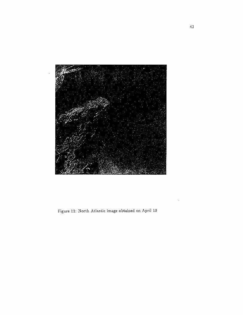
Figure 11: North Atlantic image obtained on April 10

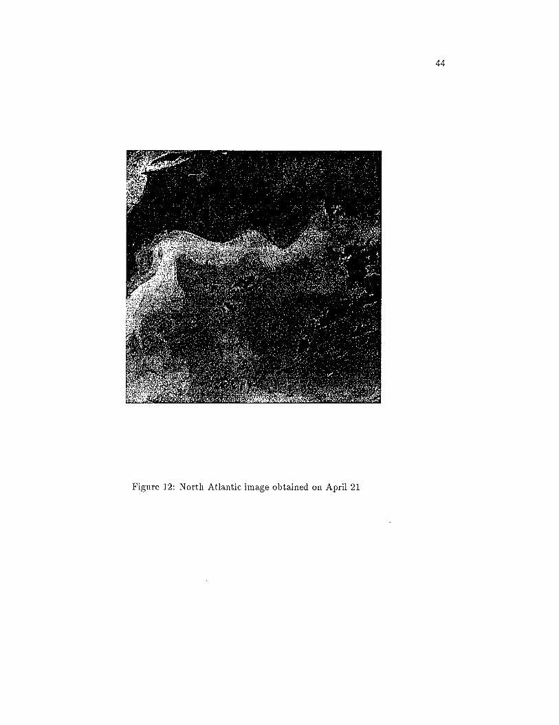
Figure 12: North Atlantic image obtained on April 21

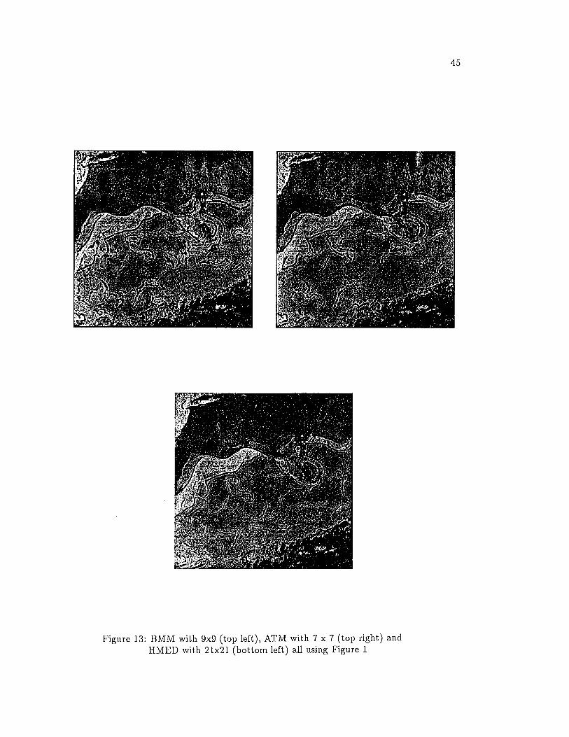
Figure 13: BMM with 9x9 (top left), ATM with 7 x 7 (top right) HMED with 21x21 (bottom left) all using Figure 1

i-i J tsLASZL- ■!. 01 -. i\.‘

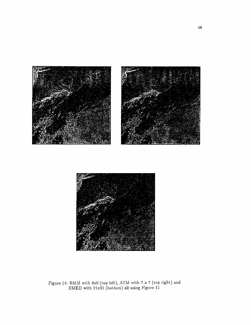
Figure 14: BMM with 9x9 (top left), ATM with 7 x 7 (top right) and HMED with 21x21 (bottom) all using Figure 11

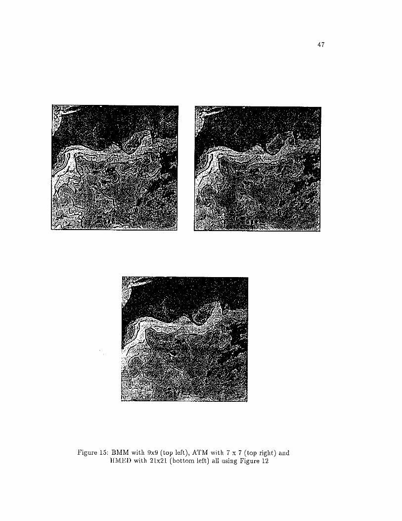
Figure 15: BMM with 9x9 (top left), ATM with 7 x 7 (top right) and HMED with 21x21 (bottom left) all using Figure 12

48

13, 15 x 15, 17 x 17, and 19 x 19. The HMED detector finds far fewer spurious edges,

and increasing the window size seems to increase the continuity of the edges without

finding many more.

Figures 11, and 12 are also satellite images of the North Atlantic. Figures 13,

14, and 15 show a com parative analysis of the three methods applied to the three

images. In each case, the results with the structuring element judged to give the

best performance is shown. All three methods find the Gulf S tream ’s North Wall

and boundaries of warm eddies, for all structuring elements. These edges have high

gradient values, so detection is relatively easy. The South Wall and boundaries of

cold eddies are spatially distributed over 6-7 pixels with low gradient values. None of

the detectors do as well in extracting these weak gradients as in finding the stronger

ones, when using small structuring elements. Increasing the size causes the BMM

and ATM detectors to introduce many spurious edges. However, the HMED detector

is able to extract these weak gradient values without introducing numy spurious edge

pixels.

Again, HMED is able to extract the boundaries of the mesoscale features without

introducing spurious edge pixels. We conclude tha t the HMED’s better performance

is due to the use of h-dilation and h-erosion.

49

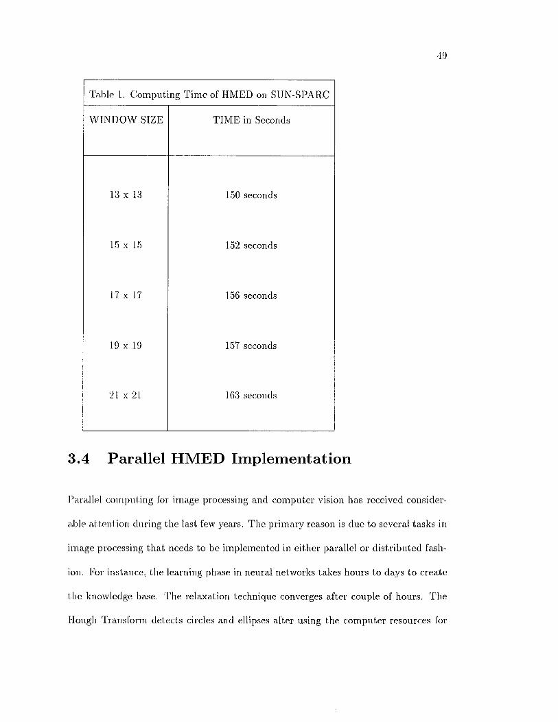
Table 1. Computing Time of HMED on SUN-SPARC

WINDOW SIZE TIM E in Seconds

13 x 13 150 seconds

15 x 15 152 seconds

17 x 17 156 seconds

19 x 19 157 seconds

21 x 21 163 seconds

3 .4 P a ra lle l H M E D Im p lem en ta tio n

Parallel computing for image processing and com puter vision has received consider­

able attention during the last few years. The prim ary reason is due to several tasks in

image processing tha t needs to be implemented in either parallel or distributed fash­

ion. For instance, the learning phase in neural networks takes hours to days to create

the knowledge base. The relaxation technique converges after couple of hours. The

Hough Transform detects circles and ellipses after using the com puter resources for

50

several minutes. The fourier transform involving huge matrices takes several minutes.

The above mentioned methods not only require prolonged use of the CPU, but also

require huge amount of com puter memory to store the image. Techniques have been

developed for sequential processors to reduce both the memory requirements and the

com putational complexity. However, further improvements can be made using paral­

lel computers. While a large number of parallel com puter architectures are designed,

very few have been built and tested with real applications. The two main exceptions

to this are mesh connected processor arrays and hypercube m ulticom puters. Both of

these schemes are commercially implemented by a number of vendors, and tested by

a large number of researchers for real applications.

Mesh connected computers are of particular interest to the image processing com­

m unity because the topology of the pixels in the image and the processors in MCC

matches perfectly and the nearest-neighbor interconnection among processors pre­

serves the spatial relation among image pixels while maintaining a low-hardware

im plem entation cost. Moreover, mesh-connected arrays can efficiently handle low

level-image processing applications which require only local operations on image pix­

els.

All Processing Elements (PEs) in MCC are arranged in a 2D rectangular grid of

size M x M where each PE is directly connected to four-neighbors, each one in North,

East, South and West direction. Thus, a PE can easily communicate to its four

neighbors. This feature is extremely suited to image processing operations such as

convolution, tem plate based edge detection in which each pixel needs the pixel value

of its four neighbors. Each PE maintains a local memory for storing da ta and receives

instructions from a centralized controller. All PEs work in a synchronized fashion un­

der a Single Instruction, Multiple D ata (SIMD) Stream mode. This means all the

active PEs execute the same instruction, but on different data. This mode of opera­

tion is needed in image processing algorithms because the algorithms predom inantly

perform the same instructions on different data sets.

3.4.1 M o t iv a t io n fo r P a ra lle l P rocessing

The motivation of designing a parallel IIMED algorithm is primarily due to the se­

quential IIMED algorithm processes a 512x512 image for almost 150 seconds on a

SUN-SPARC workstation, and this is acceptable if only one image is to be processed.

The Cluster-Shade algorithm discussed before runs lor almost 10 minutes for the same

512 x 512 image. However, this is not acceptable when a large number of images are

to be processed. This led us to investigate a possible reduction in the running time

of the HMED algorithm on a parallel machine, such as MASPAR, whose architec­

ture is similar to the MCC. We provide a brief description of MASPAR and the

implem entation of HMED on MASPAR.

MASPAR consists of 128 x 64 processors arranged in a 2 dimensional grid - with

128 processors horizontally and 64 processors vertically. The processors operate in a

SIMD fashion with the instructions provided by a centralized processor (controller).

The controller is a unix-based machine and the parallel language is called MPL which

is an extension of ’C ’ language. Each processor has an iproc to uniquely identify the

processor. A processor can be also be identified by a pair of numbers ixproc, iyproc

where ixproc is the x-coordinate and iyproc is the y coordinate of the processor. The

52

top-left processor’s iproc is 0 and ixproc, iyproc pair is (0, 0). Similarly, the bottom-

right processor’s iproc is 8192 and ixproc, iyproc pair is (127, 63). Each processor has

a local memory of 128,000 bytes.

A processor can be enabled or disabled to participate in an operation by setting

a mask. The ’lor’ statem ent given below, for instance,

if ( iprocis not 25)

Begin

do the loop statem ents

End

is executed by all processors except processor 25 or (0, 25).

if (ixprocis 45)

Begin

do the loop statem ents

End

is executed by all processors in column 45.

53

The next step involves the mapping of 512 x 512 image onto the 128 x 64 array

of processors in MASPAR. The main factors in mapping are : size of the sub-images

to be mapped and the window size to be used by HMED. HMED uses window sizes

15 x 15, 17 x 17, 19 x 19 or 21 x 21. HMED computes the gradient value of a

pixel P(x,y) using the pixels values of pixels tha t are present in a window centered

at (x,y) coordinates. We consider a few of them and discuss their advantages and

disadvantages.

We implemented a simple scheme read-block m eth o d in which each processor

is allowed to read block of pixels (or sub-image) directly from the image. The method

partitions the image into a number of sub-images and assigns each sub-image to a

processor. Each processor implements the HMED on the sub-image just, like the

sequential technique. However, the border pixels cannot be processed because of

some missing pixels tha t are present in the adjacent processors. For example, let us

consider a 32 x 32 sub-image and window size 15 x 15. A processor processes the

sub-image in middle region of size 17 x 17, but not the seven rows of pixels on top

and bottom and seven columns of pixels on left and right of the sub-image. Thus

processor exchanges the seven rows of top pixels for the bottom seven rows of pixels

in the north adjacent processor. The bottom seven rows of pixels in the sub-image

are exchanged for the top seven rows of pixels in the south adjacent processor’s sub­

image. The left seven columns of pixels are exchanged for the right seven rows of

pixels in the west adjacent processor’s sub-image. Similar exchange of pixels is done

with the east adjacent processor.

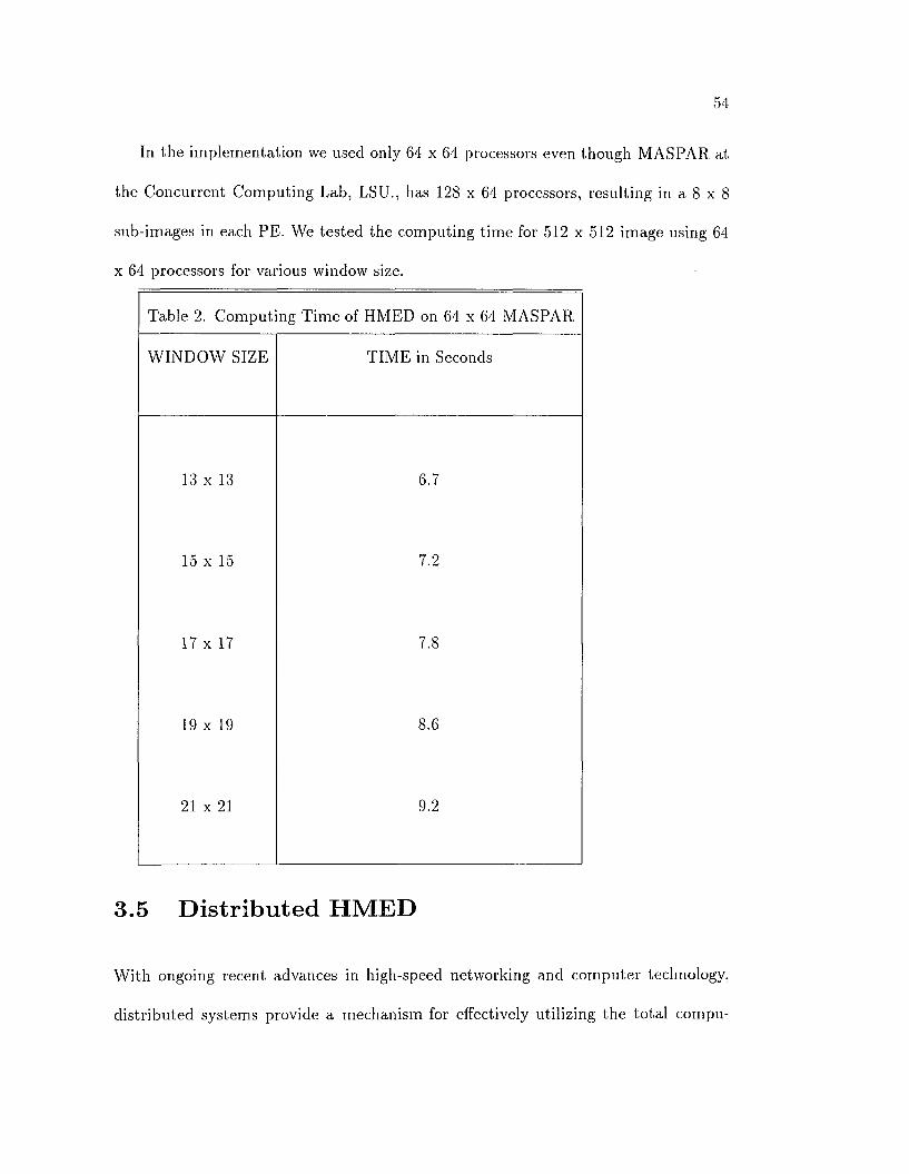
In the im plementation we used only 64 x 64 processors even though MASPAR at

the Concurrent Computing Lab, LSU., has 128 x 64 processors, resulting in a 8 x 8

sub-images in each PE. We tested the computing time for 512 x 512 image using 64

x 64 processors for various window size.

Table 2. Computing Time of HMED on 64 x 64 MASPAR

W INDOW SIZE TIM E in Seconds

13 x 13 6.7

15 x 15 7.2

17 x 17 7.8

19 x 19 8.6

21 x 21 9.2

3.5 D is tr ib u te d H M E D

W ith ongoing recent advances in high-speed networking and com puter technology,

distributed systems provide a mechanism for effectively utilizing the to tal compu­

tational power of multiple workstations available on a local network. We notice,

however, massively parallel computers and hundreds of high-performance worksta­

tions in our computing environments frequently sit idle for many hours in a day. This

led us to investigate ways of distributing the data and the time-consuming image

processing tasks to the network of workstations available to us. Unlike a massively

parallel supercom puter dedicating uniform and intensive computing power, a network

com puting environment provides non-dedicated and scattered computing cycles. The

prim ary purpose of this im plem entation is to document a pilot study using network of

machines, connected by Ethernet, to coordinate distributed image processing tasks.

Thus, we anticipate tha t using loosely coupled network of high performance work­

stations would reduce the to tal time linearly and process images tha t are too large

to process in a single machine. There exists many com puter softwares for coordinat­

ing distributed image processing tasks, such as Parallel V irtual Machines P V M , to

implement the data communications between the machines. PVM lets users write

portable application programs to execute on various workstations. To run a program

using PVM, daemon process have to initiated on the host and remote machines, and

the application program have be loaded on the remote machines. The daemon pro­

cesses guarantees reliable delivery of data between the remote and host machines.

The daemon processes also guarantees communication and coordination between the

machines.

In this pilot study, however, we use TCP-IP and UNIX-BSD sockets as a medium

of communication and coordination between the remote machines and the host. The

communication and coordination is based on the client-server model. As a result

56

we have to code the basic routines for communication and coordination between the

host and remote machines. The host machine, as a server, manages the images to

be processed and waits for the clients (remote machines) to request the data or sub­

images to process. Soon after receiving a request from a client, the server creates

another process as a child process and instructs the child process to transfer the data

to the client and receive the processed data from the client. The child process and

the client communicate through sockets created.

The server creates shared memory to store input and output images. All child

processes can access the images on a m utual exclusion (one by one) basis.

At the creation of the child process, the parent process (server) assigns next un­

processed sub-image to the child processes for transferring the data to the client. The

server itself can transfer of data, but it has to wait for requests from other clients. The

child process knows the exact location of the sub-image in the actual input image.

After receiving the data from the child process of the host server, the client execute

the IIMED algorithm on the input data. After processing the data with HMED, the

client sends the processed data back to the host machine (server).

The server program is installed in Silicon Graphics machine at Robotics Research

Lab, LSU. The clients (approxim ately 16) are spread across the entire LSU computing

services. We tested the software both during day and night times. The computing

tim e taken by the clients varied from 18 to 30 seconds. It is noted this tim e is

prim arily due to the data communication using TCP-IP.

Table 3. Computing Time of HMED on Network of W orkstations

No of Processors TIM E in Seconds

16 18-30 seconds

Chapter 4

Feature Labeling Techniques

4.1 In tr o d u ctio n

Several previous studies have addressed the autom ation of analysis of IR imagery

for mesoscale features. Gerson and Gaborski [8] and Gerson at al [9] investigate the

detection of Gulf Stream in IR images from the Geostationary O perational Envi­

ronmental Satellite [GOES]. The resolution of GOES is 8 km /pixel, while AVHRR

provides 1.1 km /pixel at nadir. Thus GEOS provides a coarser representation of

the ocean surface. Gerson and Gaborski use a hierarchical approach in which 16x16

pixel frames within a image are evaluated for the presence of a Gulf Stream . Frames

flagged as Gulf Stream possibilities are further evaluated using a 5 x 5 pixel window

within each frames. The evaluation is carried out using mean, standard deviation

and second order gray level statistics.

Coulter [6] performed autom ated feature extraction studies using the higher reso­

58

lution (1 km) AVTIR.R data. Mean, standard deviation, and gradient in a 3 x 3 pixel

window were combined with em a priori probabilities based on a large data set in

order to classify each pixel according to bayes’s decision theory. Boundaries between

water classes then became an indication of edge locations within an image. Promising

results were reported for this method for locating the Gulf Stream. However, Coulter

[6] reported tha t eddy classification is more difficult because their historical statistics

are less stationary. Indeed, the requirement for em a priori knowledge and stationary

statistics is a limiting factor in the use of this method.

Janowitz [18] studied the autom atic decision of the Gulf Stream eddies using

AVHRR data. Recognizing tha t edges in this high-resolution IR imagery are too

noisy, i.e., have too much fine-structure detail, for effectively locating eddies, Janowitz

started with filtering to smooth the image. Smoothing was followed by an image sim­

plification algorithm [18]. The smoothed and simplified image was then transformed

into a binary edge image by a Kirsch edge detector (as described in [41]. The last

step was ellipse detection on the binary edge image as a means of locating eddies.

The centers of all thess cold eddies in the test image were correctly identified and

no ecly false alarms were reported. The Janowitz study lends further support to the

feasibility of autom ated mesoscale feature detection.

Nicliol [34] uses a Region Adjacency Graph to define spatial relationships between

elem entary connected regions of constant grey level called atoms. Eddy-like struc­

ture is then identified by searching the graph for isolated atoms of high tem perature

tha t are enclosed by atoms of lower tem perature (for the case of warm eddies). Al­

though satisfactory emulation of human extraction of eddy structure is claimed for

60

this method, Nichol [34] does not point out tha t not all enclosed uniform areas iden­

tified by this method will correspond to real ocean structure. We agree with this

conclusion. It seems possible tha t relatively uniform areas such as the Sargasso Sea

tha t might be devoid of eddies could possibly contain more uniform areas than the

region near the Gulf Stream where eddies exist but the spatial patterns of the sea

surface tem perature are very complex. The ’’false alarm ” statistics of Nichol’s m ethod

should be examined.

Although these investigators have reported some success in autom ating the in ter­

pretation process for oceanographic images, they were trying to do the entire in ter­

pretation step using conventional image processing techniques.. In other words, there

was 110 sharp division between the non-semantic based modules and sem antic based

modules, partially because the knowledge-based methodology was not available to

provide the tools (Argialas and Harlow, 1990). Because of the growing need for the

incorporation of domain-specific knowledge into image analysis, and taking advan­

tage of the recent development of knowledge representation and inferring techniques,

knowledge-based systems to em ulate the human way of solving domain-specific prob­

lems have been developed

The Naval Research Laboratory began development of the Semi-Automated Mesoscale

Analysis System (SAMAS), a comprehensive set of algorithms tha t handles the entire

autom ated analysis problem, from low-level segmentation through intermediate-level

feature formation and into higher-level Artificial Intelligence modules th a t estim ate

positions of previously detected features when cloud cover obscures direct observation

in the current image set [26]. The SAMAS architecture is shown in Figure 2.

SAMAS, however, only employs feedback from the high-level modules to the

medium-level modules. No feedback from the medium to low-level is employed, be­

cause our objective is to make the low-level module independent of the domain specific

knowledge.

Feature locations produced autom atically by SAMAS compare favorably with

those from human interpreters. An im portant part of the SAMAS is the labeling

of edges or regions identified by a low-level segmentation routine. By ’’labeling” we

mean assignment of an oceanographic identity to each edge or region fragment. The

labeling is based on oceanographic knowledge of some form. The required knowl­

edge could be sea-surface tem perature values characteristic of a given feature, spatial

context {e.g. ’’north of” or ’’south of” ), a previous analysis, or any other source of

knowledge tha t helps identify features. The main modules of the SAMAS are the

segmenter, labeling module, and expert system to predict the position and size of

the mesoscale features. In the next section a brief review of the im portance of these

module in any vision systems is provided.

The current version of SAMAS groups various modules into these three categories.

A cloud detection algorithm processes the therm al infrared image of the ocean to clas­

sify all pixels either as cloud pixels or non-cloud pixels [Sonia, 1992], Considering only

non-cloud pixels, the system uses the cluster shade texture measure as the low-level

operation and detection of zero crossings in cluster shade as the medium-level oper­

ation, leading to a set of edge primitives (Ilolyer and Peckinpaugh, 1989). SAMAS

uses two-step nonlinear relaxation [20] to label edge primitives [22]. In the first re­

laxation labeling step, a priori probability values of the edge pixels are com puted

62

using a priori knowledge of the approxim ate sizes and positions of the features, based

on a previous analysis (typically from one week earlier). In the second step, these

probability values are updates using compatibility coefficients in an iterative fashion,

until the values stabilize. The relaxation labeling technique reduces uncertainty in

the assignment of labels to edge pixels [22], A rule based expert system predicts

the future position of the mesoscale features. There is a feedback from the expert

system to the medium level module. We present some previous methods th a t have

been developed: Neural Networks, Relaxation technique and Expert Systems.

4 .2 N eu ra l N etw o rk s

Neural networks are composed of many simple com putational units tha t work in uni­

son to process information. A network is not programmed in a traditional sense,

rather the weights tha t connect the neurons are ” learned” by the network through

repeated applications of input data for which the desired result is known. Neural net­

works use their massively parallel architecture to explore many competing hypothesis

simultaneously. This gives neural networks great potential for application in areas

such as speech and image recognition.

The potential benefits of neural networks extend beyond massive parallelism. Neu­

ral networks can process inexact, ambiguous, fuzzy data tha t do not exactly match

any information stored in memory. Also, compared to traditional statistical tech­

niques, neural network classifiers are non-param etric and make weaker assumptions

about the shapes of the underlying distributions than traditional statistical classifiers.

63

Neural network technique was applied to the mesoscale labeling problem. The

neural network used was a feed-forward, fully connected net with an input layer, one

hidden layer and output layer. A supervised training algorithm, back propagation,

was used in this neural network. Backpropagation uses a gradient descent search

technique to minimize the mean-squared-error between the desired output and the

actual network output. In back propagation, input patterns along with the desired

output patters are presented to the neural net. In the individual nodes of the hidden

and output layers, weights are applied to each input going into the node. These

values are then summed and evaluated using a transfer function, sigmoid function.

The value fo the transfer function on each node is passed on to the next layer. The

process is repeated until the output layer is reached. The value of the output layers

is compared with the desired output and the error is computed. This com puted error

is then propagated back through the network. This entire phase is known as training

phase. The goal of the training phase is to minimize the global error of the network

by modifying the weights. The phase continues until some user-specified values or

constraints is met. once the net has been trained, an independent test using set of

inputs is presented to the net, and the output is generated.

4 .3 R e la x a tio n T ech n iq u e

An im portant research area in image analysis and image interpretation technology is

the development of methods th a t blend contextual information with conventional

image processing algorit hms. A literature survey clearly indicates th a t such a hybrid

approach yields good results. Relaxation labeling is one such process. Relaxation

labeling has been applied to a variety of image processing problems e.g., linear fea­

ture enhancement [59], edge enhancement, image enhancement, pixel classification.

A recent survey article by K ittler and Illingworth [20] on relaxation labeling high­

lights the im portance of this area of research. The survey paper also points out the

advantages and possible applications of relaxation methods. More im portantly, the

relaxation labeling approach was elegantly described by Rosenfeld [44] who investi­

gated the problem of labeling the sides of a triangle and proposed a set of schemes

to solve the problem. They also concluded with the result tha t the nonlinear proba­

bilistic relaxation schemes yield better results than the others. Hancock and K ittler

have dem onstrated tha t probabilistic relaxation can be successively applied to edge

labeling. They also suggest two features tha t are key to the success of such a label­

ing system: firstly, a probabilistic framework to represent a world model to ensure

internal consistency, and a dictionary of labeling possibilities for the entire context-

conveying neighborhood for each object, as the second. They have shown tha t the

resulting algorithm combines evidence for the presence of edges by drawing on prior

knowledge of the perm itted label structures.

The goal of the relaxation process is to reduce the uncertainty (and improve

the consistency) in the assignment of one of the labels to each object in a set of

related objects. In the oceanographic feature classification problem, the classes are

the various oceanographic features, namely the north and south walls of the Gulf

Stream , cold eddy, warm eddy, shelf front and coastal boundary. Refer to Figure 1 to

65

identify the positions of these oceanic features in a typical image. The objects are the

individual pixels in a set of registered m ulti-tem poral images. The uncertainty could

be due to the cloud cover or the overlap of the features, features not belonging to one

of the classes, noise in the image, or other factors. In this paper, we are attem pting

to label mesoscale features, but the ocean exhibits variability on all spatial scales.

Therm al structure on scales smaller than mesoscale will interfere with the mesoscale

feature labeling process. The underlying m athem atical framework necessary for the

relaxation labeling method is described in the following paragraphs.

Let A = {Ai, A2, ..., Am} be the set of possible labels tha t may be assigned to each

pixel x in the IR image. Also we let P \ ( x ) denote the probability th a t the pixel at

x(i,j ) belongs to the object A after k iterations of the relaxation algorithm.

There are two steps in executing the probabilistic relaxation algorithm. In the

first step, a priori probabilities are evaluated with the help of ground tru th data,

a previous but recent mesoscale analysis or both. In the second step, these a priori

probabilities are iteratively updated (relaxation) until a consistent labeling is reached.

We now discuss these two steps in detail.

Step 1: E st im atin g th e a priori probabilities

Let p ° \ ( x ) denote the a priori value, tha t is, the probability th a t pixel x(i,j) belongs

to the object A at the zeroth iteration. The Bayesian probability equation is used to

evaluate this value. The equation (1) is used to calculate p ° \ ( x ) .

,\ = p (x I A) P(A)Po £ap(p(®U)

66

where p(x | A) denotes the conditional density function and P ( A) the probability of

occurrence of the object A.

To evaluate the conditional density function p(x | A), a set of param eters is m ea­

sured at the pixel x ( i ,j) . Let X denote the param eter vector. The following param e­

ters are used to form the vector X:

1. vector from origin to pixel x ( i,j) , both the m agnitude and direction.

2. gray scale intensity value at the pixel x (i,j) .

3. the edge magnitude.

For each object, the mean vector p,\ and the covariance m atrix S,\ are computed.

Also it is assumed th a t the conditional density function follows a normal distribution.

Hence the conditional density function p(x | A) is evaluated using equation (2).

p(x | A) = (2?r | £ a |)_ a e x p { - \ ( X - ^ O 'E a ’^ ~ P \ ) }

to com pute P(A), relative areas of the objects are considered. The num ber of

pixels in the object A is n\ . Then P A can be calculated using equation

P( A) nAE a n\

Step 2: Iterative updating algorithm, We now discuss the probability updating rule.

The new estim ate of the probability of A at x ( i, j ) is given by

J t+ ir - A - Pa(* ) (1 + ?* (* ))P A —

E a P a ^ ’ H 1 + 9 a ( * ) )

where q\ (x) is called the update factor.

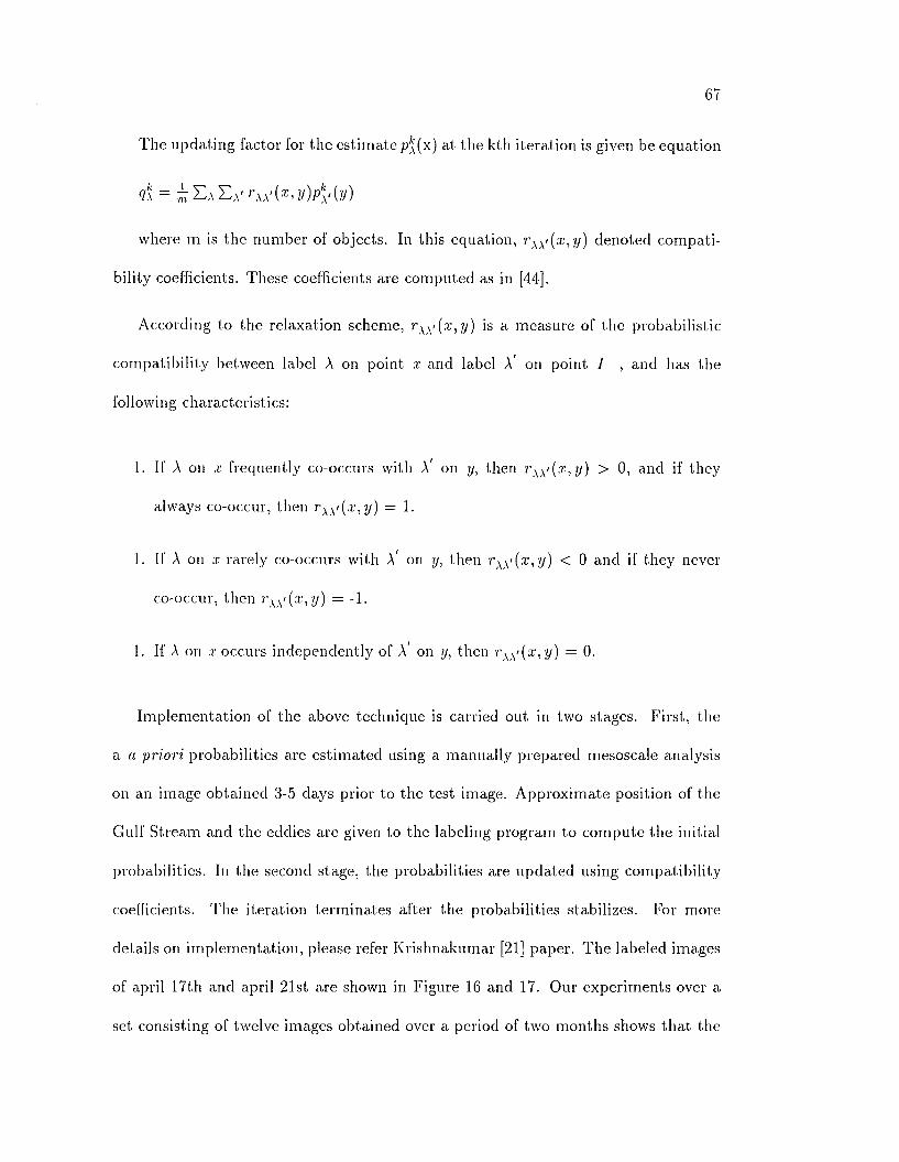
67

The updating factor for the estim ate px(x) a t the kth iteration is given be equation

(i x = £ E a E a' r w ' { x , y ) p kA v )

where m is the number of objects. In this equation, r xx>(x,y) denoted com pati­

bility coefficients. These coefficients are computed as in [44].

According to the relaxation scheme, rXX' (x, y) is a measure of the probabilistic

com patibility between label A on point x and label A* on point I , and has the

following characteristics:

1. If A on x frequently co-occurs with A’ on y, then r xx' (x, y) > 0, and if they

always co-occur, then rxy ( x , y ) = 1.

1. If A on x rarely co-occurs with A" on y, then r xx>(x,y) < 0 and if they never

co-occur, then r xx' (x, y) = -1.

1. If A on x occurs independently of on y, then r xx>(x, y) = 0.

Implementation of the above technique is carried out in two stages. First, the

a a priori probabilities are estim ated using a manually prepared mesoscale analysis

on an image obtained 3-5 days prior to the test image. Approximate position of the

Gulf Stream and the eddies are given to the labeling program to com pute the initial

probabilities. In the second stage, the probabilities are updated using com patibility

coefficients. The iteration term inates after the probabilities stabilizes. For more

details on im plementation, please refer Krishnakumar [21] paper. The labeled images

of april 17th and april 21st are shown in Figure 16 and 17. Our experim ents over a

set consisting of twelve images obtained over a period of two months shows th a t the

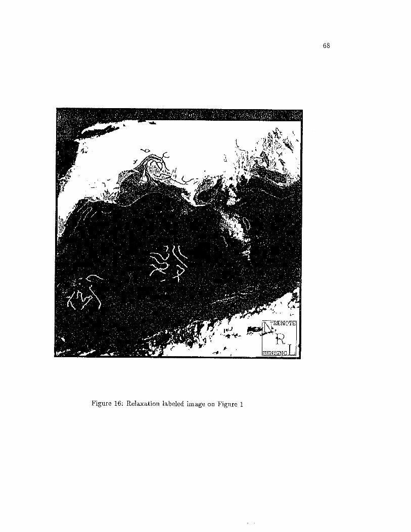
68

'REMOTE]

Figure 16: Relaxation labeled image on Figure 1

Figure 17: Relaxation labeled image on Figure 11

70

relaxation labeling module is too biased over the previous knowledge. We developed

another technique to reduce the dependence on the previous knowledge. In the next

section we discuss this technique.

4 .4 E x p er t S y ste m

In the earlier developments of knowledge-based vision systems, there was no sharp

division between knowledge based (high level, semantic) models and general purpose

(low level, non-semantic) models, partially because the knowledge-based methodology

was not available to provide the tools to do so. W ith the growing need for incorpo­

rating domain specific knowledge in image analysis, and subsequent development of

knowledge representation and inferring techniques, many expert systems were devel­

oped to em ulate the human way of solving domain specific problems.

The most popular approaches to representing the domain knowledge (both facts

and heuristics) needed for an expert system are production rules, sem antic net­

works,predicate logic, frames and blackboards. Symbolic problem solving methods,

such as modus ponens, resolution, and in-exact reasoning have been employed lor

drawing inferences. The role of the inference engine is to sequence and select the

facts in the knowledge base, m atch the extracted image features against facts, and

track inferences. The function of the controller of the inference engine is to decide

how to sta rt the inference process using the facts in the knowledge base, how to re­

solve conflicts and decide which rule to fire. There are three well known controlling

strategies: top-down, bottom -up and a combination of the first two strategies.

Top-down strategy is a goal oriented processing, where queries/hypotheses are

generated. A query may be subdivided into subqueries. For instance, a query like ”Is

there any residential area present in the image?” may be generated. The subqueries

generated may be like ’’Are there any roads present in the image?” and ’’Are there

any houses in the image?”. These subqueries are again partioned into subqueries and

so on. For the subquery ’’Are there any houses present in the image” , the system tries

to extract isolated rectangular regions invoking low-level image processing routines.

A lter extraction of these regions, a linear formation of these regions on either side of

the road is searched. If all these queries are solved, then the presence of a residential

area is inferred, stored, and used for further analysis. An example is the query ’’Are

there any water tanks present in the residential area?” . Thus, the creation of a high

level query results in the invocation of low-level image processing routines such as

region growing, shape analysis, thresholding and other routines. Top-down analysis

is extremely useful for vision systems in application where a priori inform ation about

the expected image ob jects and their relationship are available. In such circumstances,

there is a possibility of generating meaningful queries and subqueries resulting in an

efficient system.

In the bottom -up strategy, the system starts segmenting the image to find homo­

geneous regions. These regions are analyzed for shapes, intensity values, and their

relationship with other regions. These facts extracted from the low-level modules are

stored. The knowledge base is searched and matched with the facts to label the image

regions. The analysis is driven by the data at the lowest level. It is not advisable to

constraint a vision system to work purely in a top-down or bottom -up strategy.

M atsuyam a [30] developed an integrated top-down and bottom -up strategy based

expert system for aerial photographs. Goodenough [10] developed an expert system

using Prolog.

The advent of successful Artificial Intelligence techniques to em ulate the human

brain, various knowledge representation schemes and control strategies, combined

with the lack of precise m athem atical models to predict the dynamic behavior of

mesoscale leatures, has led to the investigation of the usefulness of a knowledge-

based system to predict the mesoscale features either in a sequence of images or in an

image, using a prior knowledge of the sizes and positions of the leatures in an image

obtained 3-4 days prior to the sequence of images. An expert system with a rule

base concerning the evolution of mesoscale ocean features in the gulf stream region

of the North Atlantic was developed at NRL. The essential features of the system are

discussed in brief in succeeding paragraphs.

The first and foremost step in the design of the expert system was the compilation

of knowledge pertaining to the formation, movement, evolution and decay of eddies.

The knowledge was accumulated through interviews with experts and by reviews of

the technical literature [53]. This compilation effectively forms the knowledge base of

the system. The next step was to choose an efficient representation scheme.

Rules, semantic nets, frames, blackboards are some of the efficient m edia of rep­

resenting facts. Initially, NRL developed a rule-based expert system coded in OPS83

with supporting procedures implemented in the C language. Rules are an appropriate

73

form of representing unordered knowledge, e.g, an expert knows that, a warm eddy

rotates clockwise and moves west or southwest, and a cold eddy rotates counterclock­

wise and moves southwest, with differences related to location and proxim ity to the

Gulf Stream. Currently these facts are represented in the form of rules because the

knowledge of the mesoscale features was found to be easier to represent this way.

The rule-based system ’s working memory stores the status of all known mesoscale

events, e.g, size, position, shape, etc, provided by the medium-level analysis to ini­

tialize the working memory. For purposes of rule-based com putation, the ocean is

partitioned into nine disjoint regions, each region having its own set of rules for cold

and warm eddies. An eddy’s behavior as hypothesized by the expert system depends

upon which region its center is in at the beginning of a tim e step. The expert system

has different rules for ring and Gulf Stream behavior in each of the nine geographical

regions. Basically, the motion has a region-dependent velocity vector. However, a

ring tha t is closer than a certain critical distance from the Gulf Stream undergoes a

modification of the basic motion. The Gulf Stream interaction rules are also region-

dependent. The details depend upon how close the ring is to the Gulf Stream; the

Gulf Stream interaction may result in a deflection or a looping motion, with possible

coalescence with the Stream in some cases. Ring sizes decrease with time. The rate

of decrease depends on the region and on whether there is Gulf Stream interaction.

A ring th a t shrinks below a certain size disappears. The reader is recommended to

refer to Thomason [1989] for details of the rules and the architecture of the system.

Using the initial status of the rings, the expert system updates their status.

The knowledge base of the expert system has a very simple structure. The system

models the movement of the two types of eddies in each of the nine different regions

of the Gulf Stream. The knowledge base consists of two rules for each type of eddy

in each region, giving a total of 36 rules. Each rule has a very simple left-hand side

(LIIS) th a t identifies the type of eddy and the region. The two rules for the type of

eddy in the region where its center is located are always fired. The solution strategy

is slightly different for cold and warm eddies.

The first rule for cold eddies in each region estim ates the new radius for the eddy

and asserts a fact into working memory tha t causes the second rule to fire for that,

eddy. The second rule also has a very simple set of patterns on the LIIS, but the right-

hand side (RHS) is a very long set of decisions and calculations. This procedural code

on the RHS determines the distance of the eddy from the Gulf Stream and calculates

a ratio tha t specifies the degree of intersection of the eddy and the Gulf Stream.

The change in latitude and longitude of the eddy are then predicted based on the

degree of interaction. If the interaction is negligible, then the calculation is very

straightforward. If there is significant interaction, then the degree of interaction is

used to select an interaction regime tha t is used for a more complex set of calculations.

Depending on the interaction regime selected, changes may be made in the original

value calculated for the radius, the direction of movement of the eddy, and the speed at

which the eddy travels. The rules for each region are very similar, differing prim arily

in the param eter values used in the calculations.

The first rule for warm rings in each region not only estim ates the new radius

but also estim ates the new longitude and latitude for the eddy. The RHS of the first

75

rule may also include constraints tha t model the lim itation of the movement of the

eddies by physical barriers th a t occur in specific regions. The second rule estimates

the degree of interaction with the Gulf Stream based on the revised radius, longitude,

and latitude and then makes revisions in the estim ated radius and position based on

the degree of interaction. Again, most of the decisions are made on the RHS of the

second rule in complex procedural code tha t is repeated in the rules for each region.

Chapter 5

Topography-Based Feature Labeling

Detection of topographic structures in a digital image is not a new idea. There

has been a wide variety of techniques described to detect pits, peaks, ridges and

ravines. Peuker and Johnston [39] characterize the surface shape by the sequence of

positive and negative differences as successive surrounding points are compared to

the central point. Peuker and Douglas [40] describe several variations of this method

for detecting one of the shapes from the set (pit, peak, pass, ridge ravine, break,

slope , flat). They start with the most frequent feature (slope) and proceed to the

less frequent, thus making it an order-dependent algorithm.

Johnston and Rosenfeld [19] attem pt to find peaks by finding all points P such

th a t no points in a n-by-n neighborhood surrounding P have greater elevation than P.

P its are found in an analogous manner. To find ridges, they identify points th a t are

76

either east-west or north-south elevation maxima. This is done using a “sm oothed”

array in which each point is given the highest elevation in a 2 x 2 square containing it.

East-west and north-south m axim a are also found on this array. Ravines are found

in a similar manner.

Pat on [36] uses a six-term quadratic expression in legendre polynomials fitted to

a small disk around each pixel. The most significant coefficients of the second-order

polynomial yield a descriptive label such as constant, ridge, valley, peak, saddle.

G render’s [11] technique compares gray level elevation of a central point with

surrounding elevations at a given distance around the perim eter of a circular window;

the radius of the window may be increased in successive passes through the image.

Toriwaki and Fukumara [55] take a totally different approach from all the others.

They use two local features of gray level pictures, connectivity number, and coefficient

of curvature for classification of the pixel into peak, pit, ridge, ravine, hillside.

The above mentioned techniques can be classified into two categories. In the

first category, classification is performed by operations directly on the discrete image,

whereas in the la tter, a continuous surface of a certain kind is locally fitted at each

pixel first, and classification is achieved based on this approxim ation of the underlying

surface.

We find many techniques in the literature to extract topographic labels. However,

techniques need to be developed for grouping and assembling topographically labeled

pixels to build prim itive features needed in solving practical com puter vision prob­

lems. In an independent study, notable researcher Theo Pavlidis also stressed the

78

need for grouping the topographic labels to build character recognition algorithms.

He designed several algorithms using the topographic labels and showed improved

performance in extracting characters from documents.

The digital image is an equal interval grid sampling of real values of a continuous

function, / In each neighborhood of the image the underlying gray tone intensity

function, / can be param eterized as a polynomial in row, r and column c coordinates.

A brief summary of the m athem atics of polynomial fitting within a neighborhood

follows. The reader is referred to Haralick [14] for a complete discussion. Each

neighborhood can be expressed as a cubic polynomial in r, c space.

J ( r , c) = k\ + Aqr + Aqc + Aqrq + k$rc + ksC2 + kyr^ + k^r^c T k$rc2 + A’ioc3 -

Haralick has shown tha t the coefficients Aq, Aq,. , . , . , Aqo can be expressed as linear

combinations of the intensity values within the image neighborhood. Therefore, the

coefficients can be calculated by convolution of the image with a kernal of appropriate

weights. The required convolution kernals for fitting a polynomial to a 3 x 3 pixel

neighborhood are shown in Figure 18.

After fitting, the local intensity function, /, has been fit with a polynomial, first

and second derivatives of the surface can be calculated. If we evaluate the deriva­

tives at the center of the neighborhood, he.,(r,c) coordinates = (0,0), the following

relationship between derivatives and fitting coefficients applies.

6 f / 6 r = k2

S f /S c = k3

62f / 6 r 2 = 2Aq

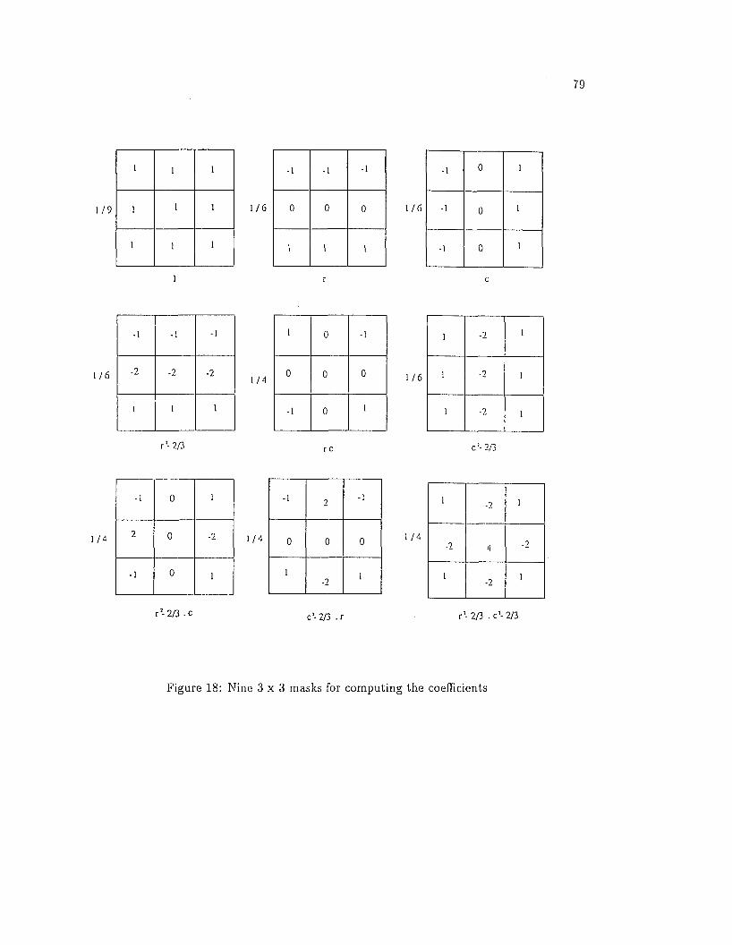
79

1 / 9

1 1 1

1 1 1

1 1 1

1 / 6

-1 -1 -1

0 0 0

1 1 1

1 / 6

- I 0 1

-1 0 1

-1 0 1

1 / 6

-1 -1 -1

-2 -2 -2

1 1 1

r 1- 2/3

1 / 4

-1 0 1

2 0 -2

-1 0 1

1 / 4

1 / 4

1 0 -1

1 / 6

1 _2 1

0 0 0 1 -2 1

-1 0 1 1 _2 1

r c o to

'—

to-1 2 -1

1 / 4

1 -2 1

0 0 0 .2 .2

1-2 1 1

-2 1

r 1- 2/3 -c c 1- 2/3 . r r :- 2/3 . c 1- 2/3

Figure 18: Nine 3 x 3 masks for computing the coefficients

80

82f / 8 c 2 = 2k(i

S2f / 6 r 6c = ks

The m agnitude of the gradient vector is then \Jk22 + k32 and its direction is

The second directional derivatives may be com puted using the Hessian

m atrix ,//, defined as

( \82f / 8 r 2 82f / S r 8c

82f /8 c 8 r 82f / 8c2 /

We know

82f / 8 c 8r = 82f / 8 r 8c

The two eigenvalues of II, Ai and A2, are the values of the extrem a of the second

directional derivatives, and their associated eigen vectors are the directions in which

the second directional derivatives are extremized (Haralick 1984).

Based on the directional derivative information, the surface, /, in a neighborhood

can be classified into one of several topographic shapes such as ridge, valley, flat,

saddle, convex hill, concave hill, etc (Haralick et .al , 1983). In the present application,

we are interested only in flat, concave hill and convex hill topographic classes.

5.1 T op ograp h ic C lassifica tion S ch em e

To classify the topographic shape at each pixel as either flat, convex hill, or concave

hill, the scheme in Table 4 is used. In the table the symbol ” + ” means significantly

greater than, means significantly less than, ”+ = ” means significantly greater

81

than or equal to and means significantly less than or equal to. Thus, ”+ = 0 ”

is read as significantly greater than or equal to zero. The symbol denotes all

other possible values. In this case no class is assigned. For example, let us consider

a pixel neighborhood and let the computed values of gradient m agnitude and second

directional derivatives Ai and A2 at center of the neighborhood (0,0) be 10, 7 and 3

respectively. Then the pixel may be classified as Convex hill. If the com puted values

12, -7 and -1, then the pixel is topographically labeled as Concave hill. If the values

are 0, 0 and 0, then we can label it as a flat. Note tha t a cloud mask is available to

the topographic classification routine which also assigns no class if any pixel within

the neighborhood is flagged as cloud covered. For example, if the center of the pixel

neighborhood is a cloud pixel, then ”No label” is assigned.

5.2 L ab elin g th e G u lf S tream

W hen the (Warm) eddy is near the (north wall of the) gulf stream , the situation poses

considerable problems to the relaxation labeling module. The relaxation labeling

module ambiguously labels some eddy pixels as Gulf Stream pixels and some Gulf

Stream pixels as warm eddy pixels. The prim ary reason is tha t relaxation technique

initializes the probability values of the edge pixels based on the distance of the edge

pixels from the previous position of the features. This a priori probabilities values

plays a vital role in the final results of the labeling module. The relaxation module

emphasizes more im portance on the previous position of the features. In doing so, the

final results seems to be more baised towards the previous positions of the features. In

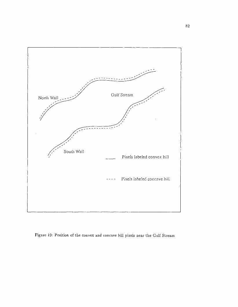
82

Gulf StreamNorth Wall

Soutli WallPixels labeled convex hill

Pixels labeled concave hill

Figure 19: Position of the convex and concave hill pixels near the Gulf Stream

other words, the error in the results of the relaxation module is directly proportional

to the errors in the previous analysis. We anticipate tha t such errors would be reduced

in our topography approach.

Experiments with a number of images have shown tha t pairs of pixels, one classi­

fied as convex hill and the other as concave hill occur along the north and south walls

of the Gulf Stream as shown in Figure 19. Spurious concave/convex pairs occur else­

where in t he image also, but these can be eliminated by a local correlation criterion.

We can also remove spurious pixels by considering only those chain of pixels which

are longer than 10 pixels. All pixels in a chain are either convex hill pixels or concave

hill pixels. A chain of pixels may be either a line, curve, arc or any other geometric

entity. Detection of these entities is tedious and cumbersome. Thus we employed a

connected component labeling and counting algorithm to extract the chain of pixels.

Thus, pairs of convex hill and concave hill classified pixels are examined initially as

possible North wall points. The criteria of examination is the gray level intensity

values. Possible North Wall points are then compared with the position of the Gulf

Stream in the previous analysis and eliminated if the distance exceeds some specified

value. It is also noted the gradient magnitude and the second directional values, Ai

and A2 , should have very high values at the North Wall. Table 5 presents the criterion

for using these values to assign North Wall labels to a pixel. In the Table 5 the symbol

”+ + ” or mean very large positive and very large negative values, respectively.

For example, if the computed values of gradient m agnitude and second directional

derivatives Aj and A2 at center of the neighborhood (0,0) are 20, 10 and 4, then the

convex hill pixel is examined for a possible North Wall pixel. Similarly, if the values

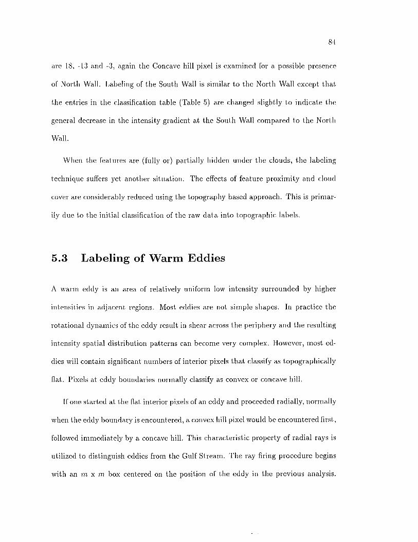
are 18, -13 and -3, again the Concave hill pixel is examined for a possible presence

of North Wall. Labeling of the South Wall is similar to the North Wall except tha t

the entries in the classification table (Table 5) are changed slightly to indicate the

general decrease in the intensity gradient at the South Wall compared to the North

Wall.

When the features are (fully or) partially hidden under the clouds, the labeling

technique suffers yet another situation. The effects of feature proxim ity and cloud

cover are considerably reduced using the topography based approach. This is prim ar­

ily due to the initial classification of the raw data into topographic labels.

5 .3 L ab elin g o f W arm E d d ies

A warm eddy is an area of relatively uniform low intensity surrounded by higher

intensities in adjacent regions. Most eddies are not simple shapes. In practice the

rotational dynamics of the eddy result in shear across the periphery and the resulting

intensity spatial distribution patterns can become very complex. However, most ed­

dies will contain significant numbers of interior pixels th a t classify as topographically

flat. Pixels at eddy boundaries normally classify as convex or concave hill.

If one started at the fiat interior pixels of an eddy and proceeded radially, normally

when the eddy boundary is encountered, a convex hill pixel would be encountered first,

followed immediately by a concave hill. This characteristic property of radial rays is

utilized to distinguish eddies from the Gulf Stream. The ray firing procedure begins

with an m x m box centered on the position of the eddy in the previous analysis.

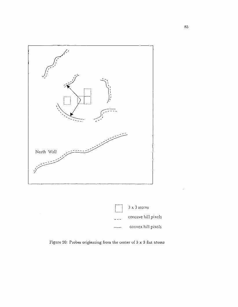
North WaH

■ i 3 x 3 atoms

concave hill pixels

convex hill pixels

Figure 20: Probes originating from the center of 3 x 3 flat atoms

86

W ithin the m x m. window all 3 x 3 areas of flat topographical class are considered

as possible eddy centers (called as atoms here). Each atom is given a counter which

is initialized to zero. From these atoms rays are sent radially in 36 directions. The

procedure is illustrated in Figure 20. Rays follow line path based on Bresenham ’s

line drawing algorithm [2]. Whenever a ray first intersects a pixel classified as convex

hill and then immediately strikes a concave hill pixel, the counter for tha t atom

is incremented. The ray is then moved to the next direction and the procedure is

repeated. If the probe does not intersect a convex hill pixel within a specified distance

(related to typical eddy size) the path of tha t ray is term inated without incrementing

the atom counter. After sending rays from all atoms and saving an accumulator for

each, the accumulators are examined for the high values indicating tha t the atom

is a possible eddy center. Any edges (i.e. convex/concave pairs) ’’visible” from the

candidate eddy centers are labeled as eddy pixels. If two candidate eddy centers are

close together, one could be selected and the other discarded based on some criterion

such as proximity to the eddy position in the previous analysis, or the atoms could

be merged into one atom located at the center of gravity of the initial atoms.

5 .4 Im p lem en ta tio n R e su lts

The edge detection and labeling capabilities of the topographical approach developed

here have been evaluated on several test images of the Gulf Stream . Polynomial

fitting window sizes 3 X 3, 5 X 5, 7 X 7 were evaluated. For a window size 7 X 7 , the

topographic classification scheme produced good results. In all of the labeled images,

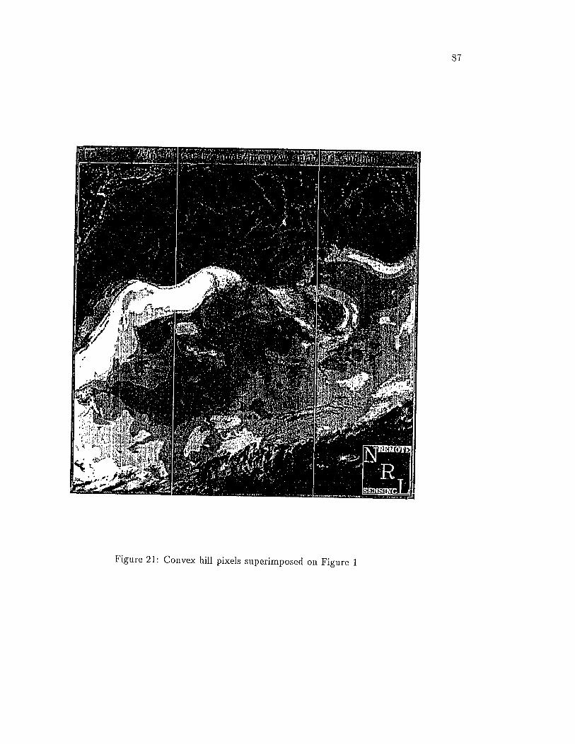
Figure 21: Convex hill pixels superimposed on Figure 1

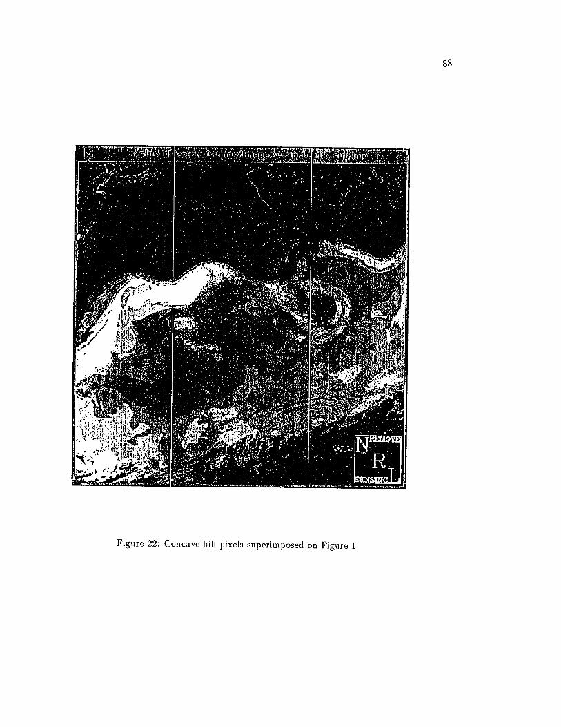
Figure 22: Concave hill pixels superimposed on Figure 1

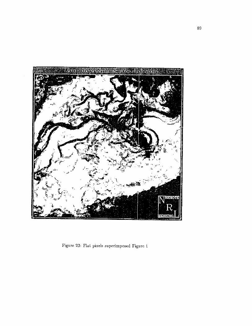
89

Figure 23: Flat pixels superimposed Figure 1

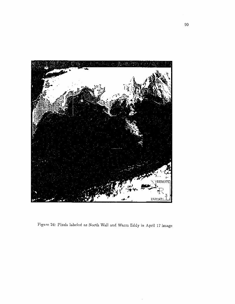
90

Figure 24: Pixels labeled as North Wall and Warm Eddy in April 17 image

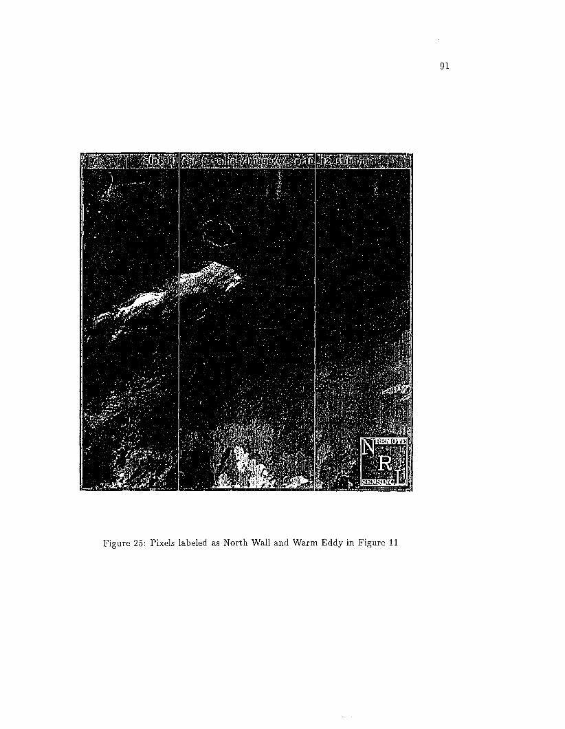
Figure 25: Pixels labeled as North Wall and Warm Eddy in Figure 11

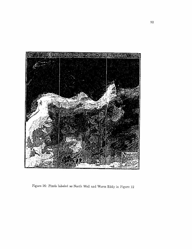
92

Figure 26: Pixels labeled as North Wall and Warm Eddy in Figure 12

93

we used a window size of 7 x 7. The technique is being tested on a number of test

images. Only chains of length 10 or more Convex hill and Concave hill pixels are

considered in order to eliminate spurious pixels. In Figure 21, the convex hill pixels

are superimposed on the original image shown in Figure 1, the concave hill pixels

are shown in Figure 22, and the flat pixels are shown in Figure 23. Figure 24 show

the pixels labeled as North Wall and as Warm Eddy. The labeled North Wall and

Warm Eddy of the Gulf Stream for Figures 11 and 12 are shown in Figures 25 and

26. The North Wall pixels are extracted from the chain of convex and concave hill

pixels by considering only intensity values of the pixels. However, by constructing a

histogram of a sub-window centered at a pair of concave hill and convex hill pixel, we

can examine the presence of a North Wall using a local thresholding technique. We

encountered some difficulties in segmenting the South Wall and the Cold Eddy of the

Gulf Stream because of very low gradient values associated with these features. At

present., we are trying to the combine the flat regions and the North Wall of the Gull

Stream to extract the South Wall.

Chapter 6

Conclusions and Future Directions

In the first part of the dissertation, we presented a Histogram-Based morphological

edge detector (HMED) blending the cues of image histogram with the morphologi­

cal operations. The new edge detector provided improved performance while being

conceptually simple and com putationally efficient. The interesting feature of HMED

is tha t it bridges two edge detection methods: histogram based methods search for

the valleys and peaks in the histogram, and the morphological methods (BMM and

ATM) search for the extreme intensities tha t have non-zero histogram heights. The

motivation of designing HMED is due to the fact tha t the previous morphological

edge detectors are designed to work only in the image domain. Such designs ignore

the vital information contained in the histogram of an (sub-)image. As a consequence,

various weak gradient values pertaining to im portant features are missed in oceano­

graphic IR images. HMED is designed to operate on the histogram of the image to

extract the weak gradients. Thus, we defined new morphological operations defined

over the histogram of a neighborhood of a pixel.

We implemented IiMED on several high-performance interconnection networks:

tightly coupled MASPAR (SIMD machine) and loosely coupled distributed network

of workstations (client-server model). We also presented im plem entation results of

IIMED on both models of architectures.

In the second part of the disseration, we proposed a general com putational frame­

work to address the problem of labeling oceanographic images. The essential ideas

stem from fitting a bicubic polynomial to each pixel’s neighborhood and assigning

topological labels based on the first and second directional derivatives of the polyno­

mial surface. The relationship between the oceanographic features in infrared satellite

imagery and the topographic structures is also presented. Our technique detects the

North Wall of the Gulf Stream and its associated Warm Eddies. We also introduced

a new algorithm to combine edge and region information for the detection of eddies.

The Warm eddies are easily extracted by this new technique. The most significant

improvement obtained by first topographically classifying the image and forming cor­

relation between topographic labels and oceanographic features is the decreased de­

pendency on the previous analysis of the features (typically one week earlier). An

added advantage of the classification scheme is th a t it can also be applied to detect

edges.

We have presented various techniques tha t exist in the literature to solve the prob­

lem of labeling of mesoscale features. We emphasize more research work is needed

to improve the autom atic interpretation schemes available today. This may be a t­

tem pted by injecting more knowledge about the scene under investigation, developing

96

powerful expert systems to assist the interpreter, and by developing new techniques

for autom atic image interpretation.

The problem of autom atic interpretation of natural scenes is quite complex and

more powerful techniques are necessary to solve this problem. Application of artificial

intelligence is shown to be one of the ways to solve this difficult problem. We em pha­

size the need for fusing both low-level and high-level knowledge usually structured as

a hierarchy of models. Expert systems certainly constitute promising tools for image

processing and interpretation.

In the two methods described earlier, namely Relaxation labeling technique and

the Topography based approach, the main characteristic nature of the eddies is ig­

nored. For instance, the eddies are predominantly either circular or elliptic or some

irregular shape. The extracted edges have to be grouped into smaller straight line

segments. Then the line segments should be grouped and tested for the presence of

eddies. Thus these techniques should incorporate the knowledge of the shape in order

to achieve better and reliable results.

Motion analysis from a sequence of time-varying images is a principal requirement

for an autom ated machine to interpret the image. Motion analysis techniques track

an object in a sequence of images using raw gradient-based schemes, edge gradient,

schemes, or feature tracking schemes. Raw gradient schemes com pute visual motion

directly from the ratio of tem poral to spatial image irradiance gradients. Edge gradi­

ent schemes com pute visual motion by matching zero crossings found in the sequence

of image. Feature tracking schemes compute motion by extracting features in one

image and search these features in the next image. Most of the motion analysis

techniques assume rigid motion of the features. However, in oceanographic images,

mesoscale features are tim e varying, i.e., mesoscale features invariably change their

position, size and shape. The problem, sometimes, is compounded by the presence of

cloud cover. Thus, the first two schemes can be rejected directly because the topology

of the edges is not preserved in consecutive images.

The applicability of the feature tracking scheme on these images with and with­

out cloud cover has to be studied. Wu [57] computed the advective velocities and

their direction from AVTIRR data using tem perature feature-tracking approach based

on pattern-m atching method. Their method is based on finding maximum cross­

correlation values within two tem plates of size 32x32 from two consecutive images.

The maximum cross-correlation approach is not suited for the application such as the

one considered in this paper because the mesoscale feature changes their direction

rapidly, in addition to the presence of cloud cover.

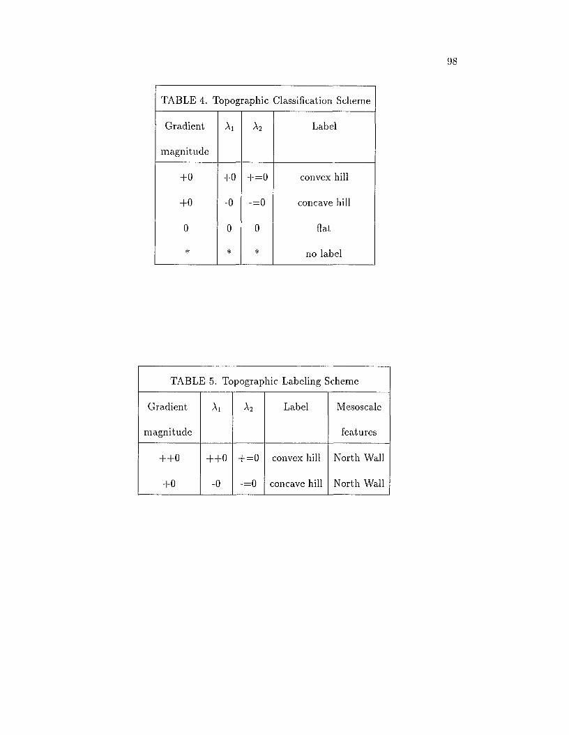
98

TABLE 4. Topographic Classification Scheme

Gradient Ai a2 Label

m agnitude

+0 +0

oII+

convex hill

+0 -0 -=0 concave hill

0 0 0 flat

* * * no label

TABLE 5. Topographic Labeling Scheme

Gradient

magnitude

Ai a2 Label Mesoscale

features

+ + 0 + + 0 + = o convex hill North Wall

+0 -0 -=0 concave hill North Wall

Bibliography

[1] D. Argialas. and C. Harlow, “Computational Image Interpretation Models: An Overview and Perspective” , Photogrammetric Engineering and Remote Sensing, 56(6), 871-886, June 1990.

[2] Bresenham, J.E ., “Algorithm for Computer Control of a Digital P lo tter” , IBM Systems Journal, 4(1), 25-30, 1965. .

[3] J.-F. Cayula, P. Cornillon, R. Holyer and S. Peckinpaugh, “Comparative Study of two recent edge-detection algorithms designed to process sea-surface tem perature fields” , IEEE Transactions on Geosci. Remote Sensing, 29, No 1, 175-177, Jan 1991.

[4] J.-F. Cayula and P. Cornillon, “Edge Detection applied to Sea Surface tem pera­ture Fields” , Proc. SPIE Tech. Symp. Optical Engg. and Photonics in Aerospace Sensing, 1990.

[5] Chan, R. and Siu, W.C, “New parallel Hough transform for circles” , lee proceed­ings. e, computers and digital techniques SEP 01 v 138 n 5 Page: 335, 1991.

[6] R.E. Coulter, “Application of the Bayes Decision Rule for A utom atic Water Mass Classification from Satellite Infrared D ata” , Proc. 17th Int. Symposium on Remote Sensing of Environment, Vol II, 1983, 589-597.

[7] F. C. Fuglister, “Cyclonic rings formed by the Gulf Stream 1965-1966” , Studies in Physical Oceanography: A tribute to George Wust on his 80th Birthday, A. Gordon, ed., Gordon and Breach, 1972, pp 137-168.

[8] D.J. Gerson and P.Gaborski, “Pattern Analysis for A utom atic Location of Oceanic Fronts in Digital Satellite Imagery” , Naval Oceanographic Office, TN 3700-65-77, October, 1977.

[9] D.J. Gerson, E. Khedouri and P. Gaborski, “Detecting the Gulf Stream from Digital Infrared D ata Pattern Recognition” , The Belle W. Baruch library in Marine Science, No. 12, 1982, 19-39.

[10] D. Goodenough, Goldberg.M., Plunkett.G ., and Zelek.J., “An Expert System for Remote Sensing” , IEEE Transaction on Geoscience and Remote Sensing, 25(3), 1987.

99

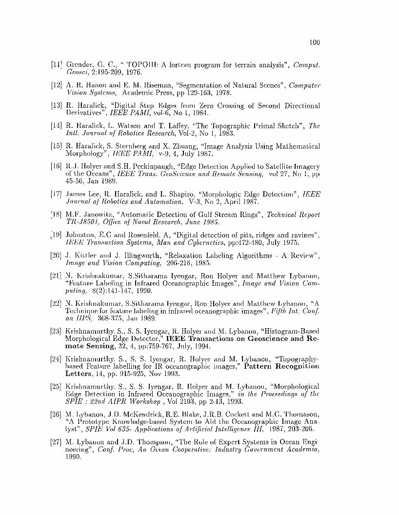
100

[11] Grender, G. C., “ TO POIII: A fortran program for terrain analysis” , Comput. Geosci, 2:195-209, 1976.

[12] A. R. Ilanon and E. M. Riseman, “Segmentation of Natural Scenes” , Computer Vision Systems, Academic Press, pp 129-163, 1978.

[13] R. Haralick, “Digital Step Edges from Zero Crossing of Second Directional Derivatives” , IEEE PAMI , vol-6, No 1, 1984.

[14] R. Haralick, L. Watson and T. Laffey, “The Topographic Prim al Sketch”, The Intl. Journal of Robotics Research, Vol-2, No 1, 1983.

[15] R. Haralick, S. Sternberg and X. Zhuang, “Image Analysis Using M athem atical Morphology” , IEEE PAMI, v-9, 4, July 1987.

[16] R .J. Ilolyer and S.II. Peckinpaugh, “Edge Detection Applied to Satellite Imagery ol the Oceans” , IEEE Trans. GeoScience and Remote Sensing, vol 27, No 1, pp 45-56, Jan 1989.

[17] James Lee, R. Haralick, and L. Shapiro, “Morphologic Edge D etection” , IEEE Journal of Robotics and Automation, V-3, No 2, April 1987.

[18] M.F. Janowitz, “Autom atic Detection of Gulf Stream Rings” , Technical Report TR-J8501, Office of Naval Research, June 1985.

[19] Johnston, E.G and Rosenfeld. A, “Digital detection of pits, ridges and ravines” , IEEE Transaction Systems, Man and Cybernetics, pp:472-480, July 1975.

[20] J. K ittler and J. Illingworth, “Relaxation Labeling Algorithms - A Review” , Image and Vision Computing, 206-216, 1985.

[21] N. Krishnakumar, S.Sitharam a Iyengar, Ron Ilolyer and M atthew Lybanon, “Feature Labeling in Infrared Oceanographic Images” , Image and Vision Com­puting, 8(2):141-147, 1990.

[22] N. Krishnakumar, S.Sitharam a Iyengar, Ron IJolyer and M atthew Lybanon, “A Technique for feature labeling in infrared oceanographic images” , Fifth Int. Conf. on UPS, 368-375, Jan 1989.

[23] Krishnamurthy. S., S. S. Iyengar, R. Ilolyer and M. Lybanon, “Histogram-Based Morphological Edge Detector,” IEEE T ransactions on G eoscien ce and R e ­m o te Sensing, 32, 4, pp:759-767, July, 1994.

[24] Krishnamurthy. S., S. S. Iyengar, R. Ilolyer and M. Lybanon, “Topography- based Feature labelling lor IR oceanographic images,” P attern R eco g n itio n L etters, 14, pp. 915-925, Nov 1993.

[25] Krishnamurthy. S., S. S. Iyengar, R. Ilolyer and M. Lybanon, “Morphological Edge Detection in Infrared Oceanographic Images,” in the Proceedings of the SPIE : 22nd AIPR Workshop , Vol 2103, pp 2-13, 1993.

[26] M. Lybanon, J.D. McKendrick, R.E. Blake, J.R.B. Cockett and M.G. Thomason, “A Prototype Knowledge-based System to Aid the Oceanographic Image Ana­lyst” , SPIE Vol 635- Applications of Artificial Intelligence III, 1987, 203-206.

[27] M. Lybanon and J.D. Thompson, “The Role of Expert Systems in Ocean Engi­neering”, Conf. Proc, An Ocean Cooperative: Industry Government Academia, 1990.

101

[28] D. Mason, I. J. Lauder, D. Rutoritz and G. Spowart, “M easurement of C-bands in human chromosomes, Computer. Biol. Med, 179-201, 1975.

[29] G. M atheron, “Random Sets and Integral Geometry” , Wiley and Sons, New York, 1975.

[30] T. M atsuyama, “Knowledge-Based Aerial Image Understanding Systems and Expert Systems for Image Processing” , IEEE Transactions on Geoscience and Remote Sensing, 25(3), 1987.

[31] D. Mckeown, W. Harvey, and J. M cdermott., “Rule-Based Interpretation of Aerial Imagery” , IEEE Trans. PAMI, 7(5), sep 1985.

[32] II. M uam m ar and M. Nixon, “Approaches to extending the Hough transform ” , Proc, ICASSP , 1556-1559, 1989.

[33] M. Nagao, “Control Structures in pattern analysis” , Pattern Recognition, vol-17, 45-56, 1984,

[34] D. G. Nichol, “Autonomous Extraction of Eddy-like Structure from Infrared Images ol the Ocean” , IEEE Trans. GeoScience and Remote Sensing, 25, 28-34, 1987.

[35] D. B. Olson, R. W. Schm itt, M. Kennedy, and T. M. Joyce, ”A two-layer diag­nostic model of the long-term physical evolution of warm-core ring 82B” , Journal of Geophysical Research, vol-90, no C5, pp 8813-8822, 1985.

[36] Paton. K., “Picture description using Legendre polynomials” , computer Graphics Image Processing, 4(1), 40-54, 1975.

[37] S. Pelag, J. Naor, R. Hartley and D. Avnir, “M ultiple Resolution Texture Anal­ysis and Classification”, IEEE Trans. PAMI, 198/f 518-523, 1984,

[38] S. Pelag and A. Rosenfeld, “A Min-Max Medial axis Transform ation” , IEEE Trans. PAMI, 206-210, 1981.

[39] Peuker, T. K., and Johnston, E. G, “ Detection of Surface-specific points by local parallel processing of discrete terrain elevation data” , Tech. Report. 206, College park, Md.: University of m aryland Computer Science center, 1972.

[40] Peuker, T. K., and Douglas, D. II., “Detection of Surface-specific points by local parallel processing of discrete terrain elevation data” , computer graphics and image processing, 4(4):375-387, 1975.

[41] W.k. P ra tt, Digital Image processing, New York: Wiley, p.489, 1978.

[42] Richard Feehs and Gonzalo Arce, “Multidimensional Edge D etection” , Proceed­ings of SPIE, Visual Communications and Image Processing II, vol 845, 285-292, 1987.

[43] P. L. Richardson, “Gulf Stream Rings” , in Eddies in Marine Science” , A. R. Robinson, Springer-verlag, pp 65-68, 1983.

[44] A. Rosenfeld, R.A. Hummel and S.W. Zucker, “Scene Labeling by Relaxation O perations” , IEEE Trans. Syst. Man Cyber, 6, 420-434, 1976.

[45] A. Rosenfeld and A. Kak, Digital Picture Processing, “ Academic Press” , 1982.

102

[46] The Ring Group, “Gulf Stream Cold-Core rings: their physics, chemistry, and Biology” , Science, vol 212 pp 1091-1100, 1981.

[47] J. Serra, “Image Analysis and M athem atical Morphological” , Acad. Press, New York, 1982.

[48] Stanley R. Sternberg, “Grayscale Morphology” CVGIP, 35, 333-355, 1986.

[49] P.K. Sahoo, S. Soltani, and A. K. C. Wong, “A Survey of Thresholding Tech­niques” , CVGIP, 233-260, 1988.

[50] H. Stommel, “The Gulf Stream: A Physical and Dynamical Description” , 2nd edition, Berkeley: University of California Press, 1965.

[51] Sonia Gallegos, J. Iiawkins, and C. F. Cheng, “A New A utom ated Method of Cloud Masking For AVHRR Full Resolution D ata Over The Ocean” , IEEE Geo­science and Remote Sensing, April, 1993.

[52] J.M . Tenenbaum and H.R. Barrow, “Experiments in interpretation-guided seg­m entation” , Artificial Intelligence, 8, pp 241-274, 1977.

[53] M. G. Thomason, and R. Gonzalez, “Database Representation in Hierarchical Scene Analysis” , Progress in Pattern Recognition, L. Kanal and A. Rosenfeld, editors, North-Holland, Amsterdam , vol 1, 1981.

[54] M. G. Thomason, “Knowledge-Based Analysis of Satellite Oceanographic Im­ages” , International Journal of Intelligent Systems, V-4, 143-154, 1989.

[55] Toriwaki, J., and Fukumura, T. “Extraction of structural information from grey pictures” , comput. graphics Image Processing, 7(1):30-51, 1978.

[56] M. Werrnan, and S. Pelag, ”Min-Max operators in Texture Analysis” , IEEE PAMI, 730-733,Nov 1985.

[57] Q. X. Wu, D. Pairm an, S. J. McNeill, “Computing Advective Velocities from Satellite Images of Sea Surface Tem perature” , IEEE Transactions on Geoscience and Remote Sensing, Vol 30, No 1, Jan 1992.

[58] S.W. Zucker, R.A. Hummel and A. Rosenfeld , “An Application of Relaxation Labeling to Line and Curve Enhancem ent” , IEEE Trans.Computer, 26, 922-929, 1977.

[59] S. Zucker, “Relaxation Labeling and the Reduction of Local Ambiguities” , Pro­ceedings of the Third International Joint Conference on Pat tern Recognition, 1976.

Vita

Sankar Krishnam urthy received his B.Tech degree at the Regional Institu te of Tech­

nology, India, in 1986, and holds two MS degrees from Louisiana State University,

Baton Rouge, LA., one in Engineering Science and the other in Com puter Science.

His research interests are in Com puter Vision, Com puter Graphics, Visualization and

Multimedia.

103

DOCTORAL EXAMINATION AND DISSERTATION REPORT

Candidate: Sankar Krishnamurthy

Major Field: Computer Science

Title of Dissertation:Tracking Dynamic Features in Image Sequences

Approved:

[ f 'Major Professor^ and chairman

EXAMINING COMMITTEE:

Date of Examination:

19th September 1994