Trade and Development: Evidence from the NapoleonicBlockade

Réka Juhász ∗

London School of Economics, CEP, CfM

This version: August, 2014

PRELIMINARY AND INCOMPLETE

Abstract

This paper uses a natural experiment to assess whether temporary protection fromtrade with the industrial leader can foster development in infant industries in followercountries. Using a new dataset compiled from primary sources, I show that regions(départements) in the French Empire which became better protected from trade withthe British for exogenous reasons during the Napoleonic Wars (1803-15) increasedcapacity in mechanised cotton spinning to a larger extent than regions which remainedmore exposed to trade. Temporary protection from trade proved to have long-termeffects. First, after the restoration of peace, exports of cotton goods in France grewfaster than Britain’s exports of the same. Second, emulation of Britain’s success wasnot inevitable. As late as 1850, France and Belgium - both part of the French Empireprior to 1815, had larger cotton spinning industries than other Continental Europeancountries. Third, within France, firms in areas that benefited from more protectionduring the Napoleonic Wars had significantly higher labour productivity in cottonspinning in 1840 than regions which received a smaller shock.

∗r.juhasz1@lse.ac.uk. I thank Silvana Tenreyro and Steve Pischke for their continued guidance and sup-port. This paper has also benefited from discussions with Francesco Caselli, Nick Crafts, Jeremiah Dittmar,Knick Harley, Ethan Ilzetzki, Gianmarco Ottaviano, Guy Michaels, Michael Peters, Thomas Sampson, DanielSturm and seminar participants at LSE and Warwick and conference participants at the Belgrade YoungEconomist Conference. Financial support from STICERD is gratefully acknowledged. French trade statisticsfor 1787-1828 were kindly shared by Guillaume Daudin. Data from the first French industrial census (1839-47) was kindly shared by Gilles Postel-Vinay. I thank Alan Fernihough for sharing the dataset on cities’access to coal, and EURO-FRIEND for sharing river discharge data from the European Water Archive.

1

1 Introduction

A long-standing debate in economics is centred around the question of how trade effectsgrowth. The idea that infant industries in developing countries may benefit from temporarytrade protection has been around since at least the 19th century. More recently, endogenousgrowth theory has uncovered mechanisms via which trade can both promote and hindergrowth (Grossman and Helpman, 1991, Matsuyama 1992, Young, 1991). This implies thatempirical work has an important role to play in determining the relative importance ofdifferent mechanisms. Historically, governments have often attempted to foster structuraltransformation by protecting infant industries from foreign competition. Both Germanyand the US industrialised behind highly protective tariff and non-tariff barriers (O’Rourke,2000). Many governments in developing countries attempted to foster industrialisation in thepost-colonial period using similar policy instruments with mixed results (Amsden, 1997 andKrueger, 1997). Despite the growing number of datapoints, the debate is no closer to beingresolved. Cross-country growth regressions have been unable to find a robust correlationbetween long-term growth and openness (Sachs and Warner, 1995, Clemens and Williamson2004, O’Rourke, 2000, Irwin, 2002).

Identifying the effect of openness to trade on development is notoriously difficult. By itsvery nature, economic openness is endogenous to the political process which implementstrade policy. In this paper, I present a setting where regional, within country variationin openness to trade is caused not by trade policy, but by exogenous events outside thecountry’s borders. In particular, I examine the development of mechanised cotton spinning,an important infant industry in the 19th century, across départements of the French Empireduring the Napoleonic Wars (1803-1815). These Wars led to a unique historical setting: as aresult of asymmetries in naval military power, blockade of Britain was implemented not vianaval blockade of Britain itself, but rather by “self-blockade” of Continental-Europe. Thismeant that Continental powers attempted to stop British and eventually “neutral” ships fromentering their ports. In contrast to Napoleon’s aims however, smuggling between Britain andthe Continent was rife. The balance of military power between Britain and France playeda key role in determining where new trading routes were set up. In this paper, I use thisvariation in the size of the plausibly exogenous shock to trade costs across the French Empireto identify the effect of protection from British competition on the develelopment of capacityin mechanised spinning.

To analyse the question of how the disruption to trade affected the development of the cottonindustry across the French Empire, I compiled two new datasets from original sources. Usinghandwritten prefectural reports from departments in the French Empire, I constructed adataset on mechanised spinning capacity (number of spindles) at the departmental level.Second, using the Lloyd’s List, I have been able to reconstruct how shipping routes betweenBritain and and Continental Europe were affected by the rupture to trade relations.

2

Cotton was the quintessential infant industry in the First Industrial Revolution. Throughoutthe nineteenth century, this sector played a key role in the industrialisation of Britain andwith some lag, Western European and American emulators. It is hard to overstate theimportance of cotton: between 1780-1860, cotton alone accounted for an astonishing 25%of TFP growth in Britain (Crafts, 1985). Though Britain and France had similar initialconditions in cotton spinning until about the 1750s, their paths diverged dramatically withthe breakthrough to mechanisation in Britain (Allen, 2009). First mover advantage mattered.In the 10 years between 1785 and 1795, the real price of fine yarn dropped to a tenth ofits previous value (Harley, 1998). British exports of cotton goods increased exponentially(Mitchell, 1988) with the primary destination being Europe, and in particular France andGermany (Crouzet, 1987).

Though blueprints and prototypes of new machines were available, adoption of mechanisedspinning across France and the rest of Continental Europe proceeded extremely slowly. In1790, Britain had 18,000 spinning jennies to France’s 900 (Aspin and Chapman, 1964). Bythe turn of the century, the technological gap between Britain and France was apparent.French spun cotton yarn was twice as expensive as that spun in Britain. The flow of tech-nology from Britain faced barriers as both the export of machinery and the emmigrationof skilled workers was banned. French produced spinning machines were double the priceof those in Britain (Crafts, 2011). Consistent with France’s productivity lag, in 1802 and1803 (on the eve of the Napoleonic Wars), imports of cotton goods made up 8% and 12% ofFrance’s total imports respectively.1

The Napoleonic Wars (1803-1815) in general, and the Napoloenic Blockade in particular(1806-13) caused enormous disruption to trade between Britain and the Continent (O’Rourke,2006). A traditional blockade would have entailed the French navy surrounding British portsin order to stop goods entering and leaving Britain. Because of the asymmetry in naval powerwhich favoured the British, Napoleon’s Blockade was instead implemented by attempting todeny British goods access onto the Continent. Importantly, trade between Britain and theContinent did not stop. Instead, trade was driven from traditionally water-borne routes tomore expensive, and more circuitous land-based routes.

There was significant regional variation in the extent to which the Blockade was successful.While the Blockade was generally well-enforced along the coastline of the French Empire,enforcement outside of France varied. This variation was driven by factors related to mili-tary strength and idiosyncratic political events. Most importantly, Napoleon was militarilystronger in Northern Europe, while the British controlled shipping in the Mediterranean.An idiosyncratic political event, the Spanish insurgency against Napoleonic rule from 1808onwards, reinforced Napoleon’s inherently weaker position in Southern Europe. For thesereasons, the Blockade was more successful along the North Sea and the Baltic than it wasalong the Iberian Peninsula and in the Mediterranean. In fact, in some years, British trade

1See Appendix C for details on French trade statistics.

3

with the Mediterranean and Spain surpassed pre-Blockade levels (Crouzet, 1987).

Variation in the success of the Blockade meant that traditional routes to French départementswere interrupted to a different extent. With direct trading routes between Britain and Franceeffectively closed across the French Empire, British cotton yarn destined for French marketshad to be smuggled via more circuitous and more expensive routes driving up the price atwhich competing British yarn entered a given department. Smuggling of British goods inthe North generally took one of two difficult routes, while smuggling via Southern Europewas far easier. I show evidence that, consistent with smuggling capacity constraints in theNorth during the Blockade, down-river transportation (in the South-North direction) alongthe Rhine increased dramatically.

During the Blockade, spinning capacity in the French Empire quadrupled. However, thisnumber masks significant regional variation. While some areas, notably departments alongthe English Channel, prospered, others in particular in the South and South-West of theEmpire, stagnated or declined. My identification strategy uses the trade shock as a proxyfor the shock to British yarn prices across the French Empire. Using a difference in differencespecification, I find that higher protection from trade with Britain had a large and significanteffect on the adoption of mechanised cotton spinning. Moving from the 25th to the 75thpercentile of the shock leads to a predicted increase in spinning capacity per capita that isroughly equal in size to the mean spinning capacity per capita at the end of the Blockade,a sizeable effect.

Despite the enormous disruption to trade with Britain across the Continent, producers wereable to import the raw cotton needed for production. The reason for this was that whileBritain monopolised supply of cotton yarn, they were never able to monopolise supply of rawcotton. I show that firms in France had access to Brazilian, American and Levantine cottonthroughout the Blockade, though raw cotton prices on the Continent were higher than thosein London.

My identification strategy relies on there being no other shocks contemporaneous with, andcorrelated to the distance shock. I show that the estimated effect of the trade shock isvirtually unchanged when adding time-varying controls for geographic fundamentals such asaccess to fast-flowing streams and proximity to coal. I demonstrate that the trade shock hasno similar effect for two other industries which were not affected by technological changeand whose goods are less intensively traded with the British - wool and leather. The otherunderlying assumption of the difference-in-difference identification strategy is that of parallelpre-treatment trends. I construct a measure of spinning capacity in the period prior to theNapoleonic Wars to show that the distance shock caused by the disruption to trade had nosignificant effect on spinning capacity prior to the treatment period.

The second set of results examine the longer-term effects of temporary protection from trade.

4

I examine persistence along three dimensions. First, I show that exports of cotton goods fromFrance increased after peace was restored on the Continent in 1815 relative to British exportsof the same. This shows that the increase in spinning activity during the Blockade did morethan scale up an inefficient industry which was unable to compete at world prices. Second,I show that emulation of Britain’s success was difficult and far from inevitable. Using rawcotton import data as a proxy for the size of domestic spinning industry, I show that in 1850,35 years after the end of the Blockade two countries, Belgium and France (both part of theFrench Empire) had larger cotton spinning industries than the rest of Continental Europe.Third, using firm-level data from the 1840s, I show that the trade shock had persistent effectson within country outcomes in France in the sense that firms located in departments thatreceived a larger shock had higher productivity than firms in departments which received asmaller shock.

Theoretically, the result that tariff protection can increase the growth rate of the economydepends on the existence of a market imperfection which prevents entrepreneurs from enter-ing new, “high-growth” sectors.2 Particularly relevant in this historical context is the rolethat learning-by-doing (LBD) externalities play. In a world where LBD externalities are theengine of growth, a country can remain permanently stuck in low-growth sectors. Potentialentrepreneurs do not internalise the effect that increasing production today would have onthe industry-wide cost curve. As they are not competitive at free trade prices today, they donot enter the sector, and will remain uncompetitive in the future. Protection, by increasingthe domestic price, makes entry individually profitable. As cumulative production increases,productivity increases via the learning externality, the country moves down its industry widecost curve, and firms become competitive at world prices.

LBD externalities, tariff protection and growth have been extensively debated in the lit-erature in relation to the cotton industry in the 19th century, particularly for the case ofthe US.3 Learning externalities are plausible in this setting for at least two reasons. First,cotton was the first industry to mechanise and adopt factory production on a mass-scale.The organisation of the flow of work, the division and management of labour changed rad-ically. Small, productivity enhancing improvements in production techniques in one placewere rapidly adopted by other firms (Mokyr, 2009). Second, the ban on exports of machin-ery and workers from Britain during this time period limited direct technology flows fromthe industrial leader. Would-be adopters had to build and repair the machines domesti-cally. Experimentation via production had an important role to play in driving productivityimprovements.

2Grossman and Helpman (1991) use externalities in R&D, Rodrik (1996) presents a multiple equlibriamodel with coordination failures, Krugman (1987), Matsuyama(1992), Lucas (1988) and Young(1991) presentmodels of endogenous growth with learning by doing externalities.

3On this debate see Taussig (1931), David (1970), Harley (1992), Irwin and Temin (2001) for the US.Crouzet (1964) discusses the effect that the French Revolutionary and Napoleonic Wars had on infantindustries in Continental Europe.

5

The paper is structured as follows. The next section provides the historical context. I thendevelop a very simple framework to guide the empirical analyis. The third section presentsthe data collected. Identification is discussed in the fourth section. The fifth and sixth sectionpresent the short term and long term results respectively. The final section concludes.

2 Historical context

2.1 The cotton industry in Britain and France

Asian cotton cloth was initially introduced to the European market by merchants in the 17thcentury to enormous success. Cotton’s immense popularity has been attributed to the factthat cotton printers were able to make bright, lively coloured fabric with complex patterns,something which could not be done with indigenous European textiles such as wool, linen orsilk (Chapman and Chassagne, 1981). The production of cotton cloth can be can be brokendown into four steps. First, the fibre is prepared - it is cleaned, carded and combed intorovings. The second step involves spinning the rovings into yarn. The rovings are twisted, asthis is what imparts both strength and versatility to the yarn. In the third step, yarn is woveninto cloth. The type of cloth will depend on how fine the yarn is and whether it is mixedwith other fibres. Finally, the cloth is coloured and may be printed with designs. With theexception of printing, all steps of the production process were traditionally organised rurally,meaning that spinners and weavers generally worked in their own homes.

The boom in the consumption of cotton cloth led to a fierce backlash from traditional textileindustries in both Britain and France. To a certain extent, these vested interests were ini-tially successful, as both countries banned imports of Asian cloth for domestic consumption.Furthermore, both countries banned the wearing of clothing made from cotton.4

However, two important loopholes to the general ban on cottons in both countries served asearly catalysts in the various stages of production in the cotton industry. First, domesticcotton production was tolerated. O’Brien et al (1991) argue that the ban on imported Asiancloth was instrumental in the foundation of domestic industry as it would have been difficultfor European producers to compete with Asian cloth either in price or in quality. As cottoncloth produced domestically could not be sold in domestic markets, it was initially used tobarter for African slaves (Allen, 2009).

Second, most important European port cities imported plain cotton cloth from Asia as Eu-4O’Brien et al (1991) discuss the political economy of the cotton industry in both countries in the decades

leading up to the beginning of the mechanisation process.

6

ropean spinners and weavers could not initially match the quality of Asian cloth.5 Chapmanand Chassagne (1981) document direct linkages between involvement in cotton printing andthe formation of backward linkages to cotton spinning in both countries.

In 1750, Britain and France, the two leading cotton producers on the Continent, spun about3 million pounds of yarn a year - a modest sum compared to Bengal’s 85 million poundsof output (Allen, 2009). In both countries, the size of the cotton industry was small inrelation to the size of traditional textile industries such as linen and wool.6 It would thusseem that up to the mid-eighteenth century, there was little distinction between Britain andFrance’s cotton industry and both were marginal producers. From this perspective, it ishard to overstate the extent to which the mechanisation of spinning (and later the otherstages of production) revolutionised the cotton industry in Britain. According to Crafts’(1985) calculations, cotton alone accounted for an astonishing 25% of TFP growth in Britishindustry between 1780 - 1860, for 22% of British industrial value added and 50% of Britishmerchandise exports in 1831.

The invention and subsequent development of three successive spinning machines and theintroduction of the factory system in spinning drove initial productivity improvements anddecreases in the price of yarn. The idea behind each invention was similar. Handspinningrequired one worker to operate a single wheel. The challenge was to come up with a machinethat would spin multiple rovings simultaneously, thereby increasing the output of a worker.Capacity in mechanised spinning is thus measured by the number of spindles a machine has,where a spindle is the piece of equipment which twists a single roving. The more spindles amachine has, the more rovings it is able to simultaneously twist into yarn.

Two points are worth noting about the period starting in the 1760s. First, blueprints andprototypes of each machine appeared in France soon after their invention in Britain, yet theywere not adopted on a wide scale before the Revolution. Second, the British attempted toblock technology transfer by banning exports of machinery and engineers.7 This is particu-larly interesting from our point of view, as this means that while the French easily acquiredthe blueprint for each technology, they didn’t have wide scale access to the tacit type ofknowledge that is acquired via learning by doing and that would be embedded in the exportof machines or engineers.

5This was true for handspinning, the only technology available at the time. The same was initially truefor machine spun yarn, but as a result of continuous improvements in productivity, British machine-spunyarn outcompeted the finest Indian yarn by the end of the Napoleonic Wars (Broadberry and Gupta, 2006)

6For example, Chabert (1949) estimates the size of the industries in 1788 and 1812 in France for textilesas follows (in millions of francs). 1788: Linen and hemp: 235, Wool: 225, Silk: 130.8, Cotton: no numbergiven. 1812: Linen and hemp: 242.8, Wool: 315.1, Silk: 107.5, Cotton: 191.6.

7Of course, men on both sides of the Channel attempted to game the system, but the risks were high.Smuggling of blueprints and machinery and emigration of engineers were both acts that could and werepunished by imprisonment. Nonetheless, emigree engineers were an important source of technology transfer(Horn, 2006)

7

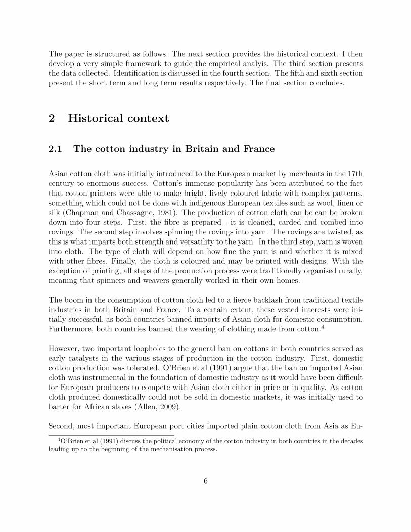
Figure 1: An engraving of a spinning jenny by T. E. Nicholson (1835)

James Hargreaves invented the original spinning jenny in the late 1760s. A picture of thiscan be seen in Figure 1. The earliest spinning jennies were hand-operated and could couldbe installed in the spinner’s home in much the same way as the spinning wheel had been.However, developments quickly led to substitution by horse, water and eventually steam-power and the organisation of work in multi-story factories.8 The spinning jenny appearedin France as early as 1771, however it was not adopted on a wide scale. Aspin and Chapman(1964) estimate that in 1790 there were 900 jennies in France, about 5% of the number inEngland.

Allen (2009) has argued that the French failed to adopt the spinning jenny on a wide scalebecause of a difference in relative factor prices. High wages in Britain rendered capital-biasedtechnological change profitable, whereas France’s lower wage economy meant that adoptionof the jenny was not profitable. However, Crafts’ (2010) careful analysis of the numbers usedin Allen (2009) reveal that differences in profitability between Britain and France seem tobe driven not by wage differentials, but by the fact that jennies are estimated to be twiceas expensive in France as in Britain. Crafts shows that French spinning would have beenprofitable at English jenny prices and also that English mechanised spinning would not havebeen profitable at French jenny prices.

8According to Allen’s estimates, the original 24-spindle jenny decreased the cost of spinning to one-thirdof its hand-value. This implied a decrease in average total cost from 35d to 31.28d in real terms. Theoriginal spinning jenny was not particularly expensive according to Allen (2009), who values it at 70 shillings(a spinner would earn a weekly wage of 8 - 10 shillings). It was however, significantly more expensive thanthe capital it replaced - a spinning wheel was valued at 1 shilling, making the original jenny 70 times moreexpensive.

8

The water-frame, patented by Richard Arkwright in 1769, was more complicated than Har-greave’s jenny, and it was predominantly this invention that led to the development ofthe factory system by the same inventor. Allen (2009) emphasises that part of the reasonthat cotton spinning proved to be so revolutionary was that for the first time, productionwas organised not rurally, in the workers’ home, but in large structures that required carefulorganisation of workflow and management of workers. The experimentation and tacit knowl-edge embedded in the water-frame and factory system is illustrated by Chapman’s (1970)finding that most cotton mills in England had a remarkably similar structure. Chapmanquotes a contemporary, Sir William Fairbairn, on the reason for this striking similarity; “Themachinery of the mills was driven by four water-wheels erected by Mr Lowe of Nottingham.His work, heavy and clumsy as it was, had in a certain way answered the purpose, and ascotton mills were then in their infancy, he was the only person, qualified from experience, toundertake the construction of the gearing.” (W. Pole (ed), 1877, quoted in Chapman (1970),my emphasis)

Finally, Samuel Crompton’s mule, which combined innovations from the jenny and water-frame was perfected in 1779, and it was this invention which dramatically increased produc-tivity as it made machine spinning of finer yarns feasible. The French were familiar withboth the water-frame and the mule-jenny, however, similarly to the jenny, they were notadopted on a wide scale. Wadsworth and Mann (1931) find that while 150 firms were usingthe waterframe in 1789, there were only 4 such firms in France and they were all significantlysmaller. In contrast to the spinning jenny, which was a simple and cheap machine, the wa-terframe and mule jenny were complicated and more expensive. Building the machines andthe factories to which they were suited required considerable skill, most of which was ac-quired by experience. This is the reason why so many of the early French firms were set upby British or Irish engineers who had acquired the necessary skills in British mills. Mokyr(2009) describes how continuous improvements in the machines and production processeswere acquired via a process of trial and error by anonymous workers and entrepreneurs.As workers were mobile between firms, and machines and factories were initially built bya handful of men as we have seen, small improvements in one firm could and did spilloverto others in Britain, but the spillover was conceivably much smaller in France, particularlybecause of the barriers erected by the government to inhibit this type of technology flow.

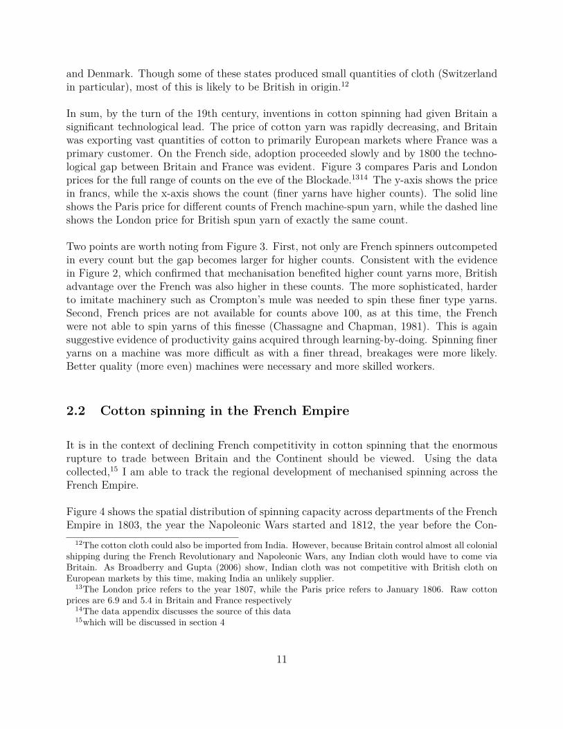
The improvements in spinning technology are reflected in the price of yarn which declinedsignificantly during the period as is shown in Figure 2. The trend is most dramatic for fineryarns, the real price of which dropped tenfold in as many years but there was also a dramaticdecline in lower count (less fine) yarns. As we have seen, historical evidence points to animportant role for learning gains in explaining part of the productivity gains. Furthermore,the very nature of these learning gains implies that they are only partially internalised by thefirm undertaking the investment and spillovers are inherent in the process. This particularhistorical setting strongly suggests that first-mover advantage in Britain is likely to makeemulation by other countries difficult as under free-trade prices they face a competitor who

9

has moved further down its industry-wide costs curve. The trade data from this periodpoints to evidence consistent with this interpretation.

Figure 2: Real price of yarn in Britain, Harley (1998)

1 Notes: Real price of cotton yarn in Britain. Mechanisation decreased price of finer (higher count) yarnsdisproportinately. For data sources see Harley (1998).

By the turn of the nineteenth century, the cotton industry in Britain was heavily export-oriented. Crouzet (1987) estimates that around 56-76% of Britain’s cotton output wasexported either in the form of cloth or yarn.9 The largest market for cotton yarn was inEurope. 44% of cotton cloth and a full 86% percent of cotton yarn exports were destined forthe European market. In comparison, only 27% of woollens and 8% of silks were destinedfor Europe. Crouzet notes that prior to the Blockade, only France, Germany, Switzerlandand Russia consumed cotton yarn.

Examining trade statistics from the French side is more challenging as imports of cottoncloth do not enter as a distinct category until after the French Revolution10 and during thetrade wars, trade statistics became highly unreliable. However, the years 1802-03 (before theBlockade) were years of general peace across the Continent when trade was relatively free. Inthese years, imports of cotton goods made up an astonishing 8% and 12% of total imports.11

By way of comparison, the respective numbers for linen and hemp together were .7% and .6%respectively and woollen textiles were not listed as an import category. The major sourcecountries for the cotton goods are listed as German states, Holland and Switzerland, the US

9As a comparison, 50% of woollens and under a third of silk was exported.10Prior to the French Revolution, textiles were categorised by type of cloth as opposed to type of material11Data sources for French trade statistics are discussed in the appendix

10

and Denmark. Though some of these states produced small quantities of cloth (Switzerlandin particular), most of this is likely to be British in origin.12

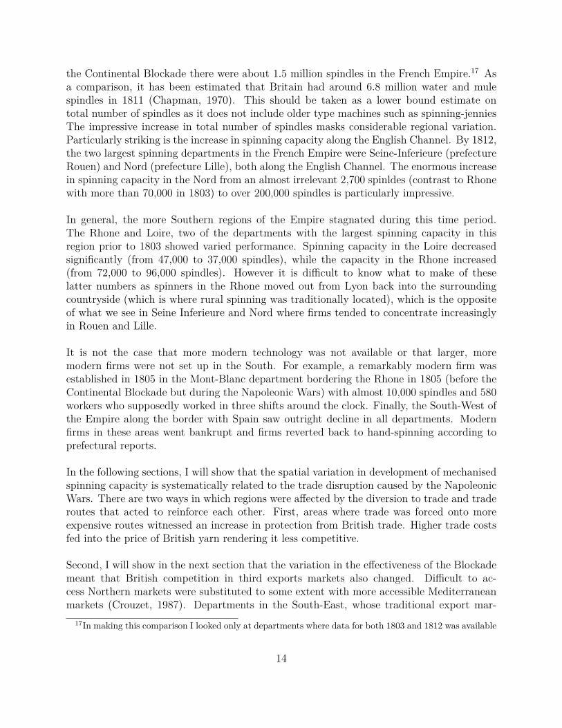
In sum, by the turn of the 19th century, inventions in cotton spinning had given Britain asignificant technological lead. The price of cotton yarn was rapidly decreasing, and Britainwas exporting vast quantities of cotton to primarily European markets where France was aprimary customer. On the French side, adoption proceeded slowly and by 1800 the techno-logical gap between Britain and France was evident. Figure 3 compares Paris and Londonprices for the full range of counts on the eve of the Blockade.1314 The y-axis shows the pricein francs, while the x-axis shows the count (finer yarns have higher counts). The solid lineshows the Paris price for different counts of French machine-spun yarn, while the dashed lineshows the London price for British spun yarn of exactly the same count.

Two points are worth noting from Figure 3. First, not only are French spinners outcompetedin every count but the gap becomes larger for higher counts. Consistent with the evidencein Figure 2, which confirmed that mechanisation benefited higher count yarns more, Britishadvantage over the French was also higher in these counts. The more sophisticated, harderto imitate machinery such as Crompton’s mule was needed to spin these finer type yarns.Second, French prices are not available for counts above 100, as at this time, the Frenchwere not able to spin yarns of this finesse (Chassagne and Chapman, 1981). This is againsuggestive evidence of productivity gains acquired through learning-by-doing. Spinning fineryarns on a machine was more difficult as with a finer thread, breakages were more likely.Better quality (more even) machines were necessary and more skilled workers.

2.2 Cotton spinning in the French Empire

It is in the context of declining French competitivity in cotton spinning that the enormousrupture to trade between Britain and the Continent should be viewed. Using the datacollected,15 I am able to track the regional development of mechanised spinning across theFrench Empire.

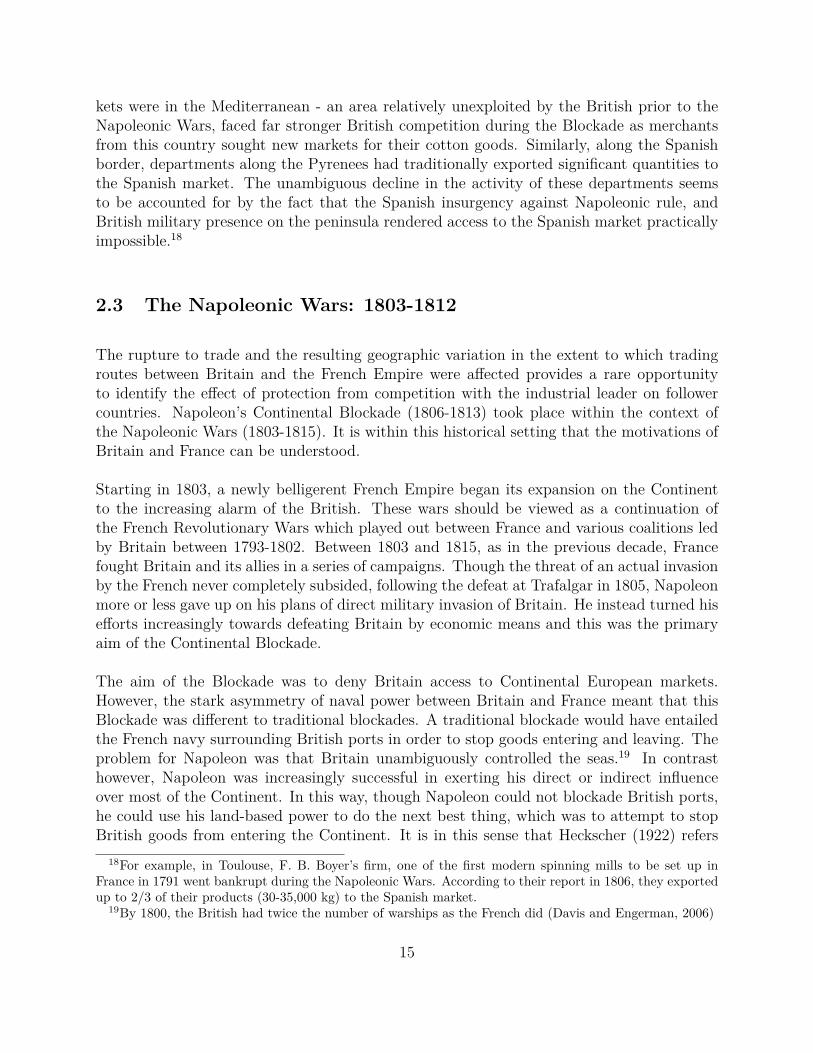
Figure 4 shows the spatial distribution of spinning capacity across departments of the FrenchEmpire in 1803, the year the Napoleonic Wars started and 1812, the year before the Con-

12The cotton cloth could also be imported from India. However, because Britain control almost all colonialshipping during the French Revolutionary and Napoleonic Wars, any Indian cloth would have to come viaBritain. As Broadberry and Gupta (2006) show, Indian cloth was not competitive with British cloth onEuropean markets by this time, making India an unlikely supplier.

13The London price refers to the year 1807, while the Paris price refers to January 1806. Raw cottonprices are 6.9 and 5.4 in Britain and France respectively

14The data appendix discusses the source of this data15which will be discussed in section 4

11

Figure 3: Price of different count cotton yarn in Paris and London, 1806-07

1 Notes: Price of machine-spun cotton yarn in Britain and France in francs by count. Finer yarn hashigher count. See Appendix C for details on sources.

tinental Blockade finally unravelled. Panel A shows the number of spindles per capita bydepartment in the French Empire in 1803 when the Napoleonic Wars began, while Panel Bgives the same for 1812 when the Blockade was unravelling 16 By 1803, many departmentshad some spinning capacity, but these firms were typically very small and they used outdatedequipment. The average firm had 440 spindles which is not more than three of four jennies.

Departments in the French Empire were affected by the developments across the Channel inmechanisation in at least two ways. First, potential spinners faced more or less competitionfrom British spinners depending on their cost-distance to Britain. Second, technology trans-fer may also plausibly be linked to distance. It is clear that these two effects work againsteach other. A potential entrepreneur along the English Channel was better placed to benefitfrom the flow of technology, but also more exposed to British competition. From this pointof view, it’s interesting to note that the departments with the largest spinning capacity (eg.Rhone and Loire in the South-East, and the Meuse south of Paris) were typically inlandmeaning they were relatively more sheltered from British competition, but also further awayfrom technology flows suggesting that the first effect may have dominated the second.

Between 1803 and 1812 spinning capacity in the Empire quadrupled. Towards the end of16I divide everywhere by departmental population in 1811 to account for the fact that some departments

are larger than others and may simply have more spinning capacity for this reason. However, the spatialdistribution of activity is similar if looked at in levels.

12

(a) Number of spindles per capita by department, 1803

(b) Number of spindles per capita by department, 1812

Figure 4: Number of spindles by department

1 Notes: Each circle gives the number of spindles per capita by department at the beginning (1803) andtowards the end of the Napoleonic Wars (1812). Circles are proportionate within, but not across thefigures. Data sources are discussed in Appendix C.

13

the Continental Blockade there were about 1.5 million spindles in the French Empire.17 Asa comparison, it has been estimated that Britain had around 6.8 million water and mulespindles in 1811 (Chapman, 1970). This should be taken as a lower bound estimate ontotal number of spindles as it does not include older type machines such as spinning-jenniesThe impressive increase in total number of spindles masks considerable regional variation.Particularly striking is the increase in spinning capacity along the English Channel. By 1812,the two largest spinning departments in the French Empire were Seine-Inferieure (prefectureRouen) and Nord (prefecture Lille), both along the English Channel. The enormous increasein spinning capacity in the Nord from an almost irrelevant 2,700 spinldes (contrast to Rhonewith more than 70,000 in 1803) to over 200,000 spindles is particularly impressive.

In general, the more Southern regions of the Empire stagnated during this time period.The Rhone and Loire, two of the departments with the largest spinning capacity in thisregion prior to 1803 showed varied performance. Spinning capacity in the Loire decreasedsignificantly (from 47,000 to 37,000 spindles), while the capacity in the Rhone increased(from 72,000 to 96,000 spindles). However it is difficult to know what to make of theselatter numbers as spinners in the Rhone moved out from Lyon back into the surroundingcountryside (which is where rural spinning was traditionally located), which is the oppositeof what we see in Seine Inferieure and Nord where firms tended to concentrate increasinglyin Rouen and Lille.

It is not the case that more modern technology was not available or that larger, moremodern firms were not set up in the South. For example, a remarkably modern firm wasestablished in 1805 in the Mont-Blanc department bordering the Rhone in 1805 (before theContinental Blockade but during the Napoleonic Wars) with almost 10,000 spindles and 580workers who supposedly worked in three shifts around the clock. Finally, the South-West ofthe Empire along the border with Spain saw outright decline in all departments. Modernfirms in these areas went bankrupt and firms reverted back to hand-spinning according toprefectural reports.

In the following sections, I will show that the spatial variation in development of mechanisedspinning capacity is systematically related to the trade disruption caused by the NapoleonicWars. There are two ways in which regions were affected by the diversion to trade and traderoutes that acted to reinforce each other. First, areas where trade was forced onto moreexpensive routes witnessed an increase in protection from British trade. Higher trade costsfed into the price of British yarn rendering it less competitive.

Second, I will show in the next section that the variation in the effectiveness of the Blockademeant that British competition in third exports markets also changed. Difficult to ac-cess Northern markets were substituted to some extent with more accessible Mediterraneanmarkets (Crouzet, 1987). Departments in the South-East, whose traditional export mar-

17In making this comparison I looked only at departments where data for both 1803 and 1812 was available

14

kets were in the Mediterranean - an area relatively unexploited by the British prior to theNapoleonic Wars, faced far stronger British competition during the Blockade as merchantsfrom this country sought new markets for their cotton goods. Similarly, along the Spanishborder, departments along the Pyrenees had traditionally exported significant quantities tothe Spanish market. The unambiguous decline in the activity of these departments seemsto be accounted for by the fact that the Spanish insurgency against Napoleonic rule, andBritish military presence on the peninsula rendered access to the Spanish market practicallyimpossible.18

2.3 The Napoleonic Wars: 1803-1812

The rupture to trade and the resulting geographic variation in the extent to which tradingroutes between Britain and the French Empire were affected provides a rare opportunityto identify the effect of protection from competition with the industrial leader on followercountries. Napoleon’s Continental Blockade (1806-1813) took place within the context ofthe Napoleonic Wars (1803-1815). It is within this historical setting that the motivations ofBritain and France can be understood.

Starting in 1803, a newly belligerent French Empire began its expansion on the Continentto the increasing alarm of the British. These wars should be viewed as a continuation ofthe French Revolutionary Wars which played out between France and various coalitions ledby Britain between 1793-1802. Between 1803 and 1815, as in the previous decade, Francefought Britain and its allies in a series of campaigns. Though the threat of an actual invasionby the French never completely subsided, following the defeat at Trafalgar in 1805, Napoleonmore or less gave up on his plans of direct military invasion of Britain. He instead turned hisefforts increasingly towards defeating Britain by economic means and this was the primaryaim of the Continental Blockade.

The aim of the Blockade was to deny Britain access to Continental European markets.However, the stark asymmetry of naval power between Britain and France meant that thisBlockade was different to traditional blockades. A traditional blockade would have entailedthe French navy surrounding British ports in order to stop goods entering and leaving. Theproblem for Napoleon was that Britain unambiguously controlled the seas.19 In contrasthowever, Napoleon was increasingly successful in exerting his direct or indirect influenceover most of the Continent. In this way, though Napoleon could not blockade British ports,he could use his land-based power to do the next best thing, which was to attempt to stopBritish goods from entering the Continent. It is in this sense that Heckscher (1922) refers

18For example, in Toulouse, F. B. Boyer’s firm, one of the first modern spinning mills to be set up inFrance in 1791 went bankrupt during the Napoleonic Wars. According to their report in 1806, they exportedup to 2/3 of their products (30-35,000 kg) to the Spanish market.

19By 1800, the British had twice the number of warships as the French did (Davis and Engerman, 2006)

15

to the Blockade as a “self-blockade”.

Figure 5 shows the political map of Europe in 1812 at the peak of Napoleon’s power. Thoughthe Emperor’s power wasn’t quite so all-prevailing in 1806, with the notable exception ofSweden, at one point or another all other European powers passed laws in line with the aimsof the blockade. By this time, the French Empire had expanded in size to include all regionsof present-day Belgium, the entire left bank of the Rhine, regions of present-day Switzerlandup to and including Geneva, and regions in the North-West of the Italian peninsula, up toGenoa. In addition, Napoleon’s relatives were on the thrones of the Kingdom of Holland,the Kingdom of Italy, the Kingdom of Naples and the Kingdom of Spain. The Portugueseroyal family had fled to Brazil and Napoleon’s relatives were also in power in key Germanstates (Connelly, 1990).

Figure 5: Political map of Europe, 1812

Historically, when Britain and France had been at war, direct trade between the two countrieshad collapsed, however the countries were able to continue trading with little interruptionby way of neutral carriers and nearby neutral ports.20 The period that I examine herediffers from other wars between Britain and France in the sense that the entire Continentwas affected. To understand the disruption to trade, it is worth examining two periodsseparately; the 3 years leading up the imposition of the Continental Blockade (1803-06), andthe the Blockade (1806-13) itself.

Disruption to trade along the North-Sea ports began in 1803 with the onset of the NapoleonicWars. “Neutral” ports along the North-Sea (Hamburg in particular), together with Dutchports had been traditionally used to continue trading with the British in times of war.However, in a highly symbolic event, Hanover (the royal dynasty to which monarchs ofGreat Britain belonged to) was occupied by the French army. Britain retaliated by imposinga tight blockade of the entire North Sea coast between the Weser and the Elbe, which was

20Figure shows that this is the case during the French Revolutionary Wars (1793-1802).

16

then expanded to include ports along the French Channel and the North Sea in 1804 (Davisand Engerman, 2006). Crouzet (1987) considers this period a prequel to the Blockade inthe sense that trade to Northern Europe was forced onto land routes for the first timesignificantly driving up the price at which goods entered the Continent. Goods were takenfrom Britain to Altona and Tonning (both North of Hamburg). They were then smuggledinto Hamburg and taken into Northern Europe via land routes.

The Continental Blockade prohibiting the entry of British goods onto the European Conti-nent was declared in Berlin in late 1806 following the defeat of the Fourth Coalition againstFrance in Jena - Auerstadt. Prussia and Russia, two allies of the British, were forced toimplement the Blockade along their coastline. It is generally believed that the outline ofthe decree had been planned well in advance of the British Orders in the Council whichthe French used as a pretext on the basis of which to retaliate. The Orders in the Council,declared earlier in 1806, had widened the blockade already in place further west to the homeof the French Navy’s Atlantic fleet in Brest. The historical events that followed the introduc-tion of the Berlin Decree are fairly complex and they involve much back and forth retaliationbetween Britain and the French, the details of which are not relevant for my purposes.21 Thefollowing points are worth noting regarding the implementation of the Blockade. (1) Theseries of laws passed by Britain and France had the effect of completely wiping out neutralshipping. Neutral carriers such as the US found themselves in violation of one or the otherpowers’ decrees which made capture by Britain or France almost inevitable. (2) The extentto which Napoleon could ensure successful implementation of the Blockade depended on hisability to keep areas outside of France under his control.

To what extent was the Blockade successful? Figure 20 shows both the dramatic disruptionto trade in general, but also the ports which remained open to British smuggling. Panel Ashows number of ships arriving from and sailing to Britain for a given port in 1802, the oneyear of peace during this period, while Panel B shows the same information for 1809, a yearduring the Blockade. Consistent with evidence from trade statistics, in 1802, as in otheryears of peace, Northern Europe and the Iberian peninsula were Britain’s primary tradingpartners with the Mediterranean playing only a secondary role. In stark contrast, in 1809,with the notable of exception of Gothenburg in the Baltic, and Heligoland in the North Sea,trade with the Northern regions of the Continent collapsed. In the South however, trade withthe Iberian peninsula continued in an almost uninterrupted way, and a further significantsmuggling port in the Mediterranean, Malta, had emerged.

This snapshot is representative of the way the Blockade played out. In general, outside ofthe coastline of the French Empire, where the Blockade was generally effective, for mostyears, the Blockade was more successful in the North Sea and the Baltic than it was in theIberian peninsula and the Mediterranean. There are two main reasons for this. (1) Napoleonwas militarily stronger in the North of Europe, particularly after his defeat of both Prussia

21The interested reader can consult Davis and Engerman, (2006).

17

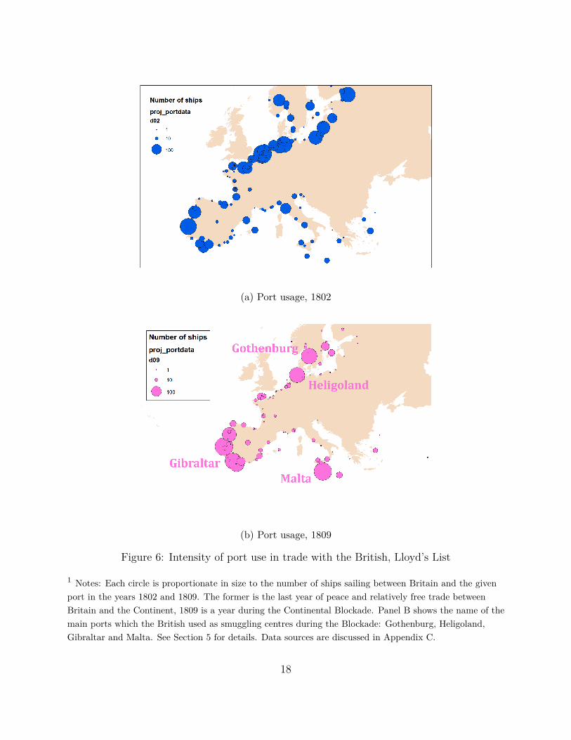
(a) Port usage, 1802

(b) Port usage, 1809

Figure 6: Intensity of port use in trade with the British, Lloyd’s List

1 Notes: Each circle is proportionate in size to the number of ships sailing between Britain and the givenport in the years 1802 and 1809. The former is the last year of peace and relatively free trade betweenBritain and the Continent, 1809 is a year during the Continental Blockade. Panel B shows the name of themain ports which the British used as smuggling centres during the Blockade: Gothenburg, Heligoland,Gibraltar and Malta. See Section 5 for details. Data sources are discussed in Appendix C.

18

and Russia in 1806. In contrast, he was inherently weaker in the South, where Portugalhad always been a reluctant ally and shipping on the Mediterranean was controlled for mostpart by the British navy. (2) An idiosyncratic political event, the Spanish insurgency, whichbegan in 1808 further weakened Napoleon’s power on the Iberian peninsula.

In practice, to smuggle successfully on a large scale, the British needed reliable access toports close to Continental Europe. From these centres, they then used ships sailing underdifferent flags with forged papers, or small fishing boats in the case of Heligoland to gettheir goods onto the Continent. For this reason, they used ports or islands that they eitherdirectly controlled (Malta, Gibraltar, Heligoland) or ports which belonged to consistentallies (Gothenburg). In this way, even if events prevented entry onto the Continent (such asperiods where Prussia and Russia consistently denied ships sailing from Scandanavia entryinto Baltic ports) goods were not lost, destroyed or taken as prize.

2.4 The shock to the price of imported raw cotton

The shock to imported British yarn prices was not the only way in which cotton producerswere affected by the disruption to trade. The period of the French Revolutionary andNapoleonic Wars also affected supplies of raw cotton within the French Empire. This sectionexamines how producers were able to secure access to raw cotton inputs during the Blockadeand the price at which they were able to do so. The shock to raw cotton inputs differed fromthe shock to British yarn prices in two important respects.

First, the source of competing yarn was Britain, while there were numerous suppliers of rawcotton. The aim of the Blockade was to stop trade with Britain. This meant resisting theentry of both British goods (industrial products such as cotton yarn) and British re-exports(colonial products such as raw cotton). Access to supplies of raw cotton were disrupted toa far smaller extent partly because the source of much of this trade was not Britain andsecond, because when one supplier was affected directly by the Blockade, substitution waspossible.

Second, both prior to, and during the Blockade, regions within the French Empire had fairlysimilar access to raw cotton. During the Napoleonic Wars, prices across the Continent werehigher than in London and this was true for the French Empire. French raw cotton prices werehigher for two reasons. First, British dominance of the seas meant that Continental producershad more difficulty in accessing raw cotton and trading routes became more circuitous andexpensive. This was a spillover effect from the blockade against British goods. Second, inthe case of the French Empire, Napoleon imposed tariffs on the imports of raw cotton, whichafter 1810 became practically prohibitive for some varieties, driving prices even higher. Ishow that French prices were within the range of prices in Leipzig - the city which becamethe centre of the cotton trade during the Blockade, until 1810 when there was a marked

19

increase in import tariffs on raw cotton.

It is somewhat paradoxical, that of of all textiles manufactured within the French Empire,cotton was the only one singularly reliant on an imported input traded via sea-routes. Forsilks, woollens, linen and hemp there was ample domestic supply of raw material and neigh-bouring countries also produced significant quantities. This was not the case for cotton wool,and it also explains why Napoleon was never fully supportive of the increase in the spin-ning capacity in cotton spinning. Heckscher (1992, p. 272) notes “ (...) there was no pointwhere the two opposing tendencies of the Continental System were so much in conflict withone another as here; and the reason was, of course, that the industry was based on a rawmaterial which was for the most part unobtainable by other means than by the forbiddenroute across the seas.” On the one hand, increasing domestic production in cotton meant aweakening of Britain’s economic advantage, however, the fact that the industry was relianton an imported input meant that the industry would always remain reliant on sea-bornetrade, strengthening Britain’s economic position.

This point should be taken into consideration when thinking both about the importanceof state support for the cotton industry. Heckscher recounts that Napoleon was constantlytrying to find substitutes for cotton. As early as 1809, he declared that “it would be betterto use only wool, flax and silk, the products of our own soil, and to proscribe cotton foreveron the Continent” (Heckscher, 1992 p. 277). In 1810, he offered a prize of one million francsfor the invention of a flax-spinning machine. Even later, in 1811, when the cotton industryfaced a sever crisis as a result of the high tariffs put in place in 1810, he banished all cottongoods from the imperial palaces.

This section shows evidence that while raw cotton was indeed effected by the disruption tosea trade, both in terms of access to raw cotton and prices, the effect of this was fairly evenacross the Empire. I first discuss the source of raw cotton and then turn to examining theprice at which firms had access to it.

2.5 Source of cotton wool

During the nineteenth century, cotton wool had been imported from three main sources:European colonies, the Levant and starting from around 1790, the US. Colonial and Americansupplies of cotton made their way to France by way of Atlantic trade, while Levantine cottonwas transported to France across the Mediterranean. Detailed trade statistics reveal thatprior to the French Revolution, about 40-50% of the cotton used in France was importedfrom the Levant, about 50% came from French Colonies, and around 10% was importedfrom Portugal, the supplier of Brazilian cotton to Europe 22 French colonial supplies of raw

22Sources for these numbers are found in Appendix ??.

20

cotton were abundant and of a high quality. In fact, Edwards (1967) discusses the fact thatas late as the 1780s, British spinners felt French spinners had an advantage because theyhad greater supplies of good quality raw material.

Shipping cotton from across the Atlantic (as was the case for colonial and later US cotton)or the Mediterranean was not particularly expensive. Harley, (1998) shows that a pound ofraw cotton, sold in the US for 12 pennies, was shipped to Liverpool for 1,5 pennies. However,overland transportation to Manchester - a mere 50km journey, cost half a penny in 1787.Given the different geographic location of various suppliers of raw cotton with respect toFrance and the access to cheap sea-trade, it would seem that within France, regions furtherinland had somewhat costlier access to raw cotton, but otherwise there was little in termsof access to imported inputs to differentiate different regions.

Two significant changes in access to supplies of raw cotton took place with the onset ofthe French Revolutionary Wars in 1793, one negative and one positive. First, France lostaccess to its colonies as a results of British naval dominance (Grab, 2003). France wouldnot be able to directly access her colonies until after 1815. Second, from about 1790s, theUS started to export growing quantities of cotton. Between 1790 and 1815, cotton exportsfrom the US grew more than tenfold. Furthermore, the Americans took on an increasing rolein re-exporting colonial products that France and her allies no longer had direct access to(Johnson et al, 1915). Growing exports of US cotton and their involvement in the re-exportof colonial products were able to substitute for the loss of access to colonies until around1808.

Table 1 gives an idea of the extent to which direct shipping was affected by the wars betweenBritain and France during our period of interest. The table is constructed using Frenchimport data, which gives details on the source country. When American cotton enteredFrance by way of Germany for example, the source country is listed not as the US, butrather as Germany. Therefore, these numbers give an idea of the extent to which cottoncould enter France in given years by way of sea-transport, and the extent to which it neededto take indirect routes. The table makes clear that up to 1808, US and Brazilian cotton(the latter re-exported via Portugal) seems to have been shipped directly to France withoutparticular difficulty. Prices did not dramatically increase until after 1808, as I will show inthe next section. This is consistent with the timeline of events. Until 1808, Portugal was anally of France - albeit a reluctant one. Furthermore, the US was a neutral carrier exportingboth its own and colonial supplies of cotton to France and Britain up to the declaration ofthe Jeffersonian embargo in 1808.

The political and military situation for both countries changed in 1807-08 making direct ac-cess to French markets difficult. Portugal, who had always been a reluctant ally of Napoleon,was finally able to switch allegiances with the outbreak of the Spanish insurrection in 1808,and this resulted in a severing of economic ties. From 1808 until the end of the Blockade

21

Table 1: Share of total importsarriving directly from source,1803-13

Direct Imports from ProducerUS Portugal Levant

1803 30 23 101804 32 35 91805 21 36 1018061807 29 45 51808 6 21 31809 0 0 71810 1 0 311811 5 0 301812 9 0 111813 24 0 20

The table gives Portuguese, US andLevantine cotton arriving directly fromeach country as a share of total im-ports of raw cotton to France in a givenyear. Direct shipping from Portugal(source of Brazilian cotton) and theUS becomes increasingly difficult af-ter 1808, as the numbers ckearly show.Direct shipping refers to imports ofcotton wool which have the produc-ing country as the source. In the caseof Portugal, it is referred to as the“source” for Brazilian cotton, as allcotton passes through Portugal. Seeappendix C for sources

in 1813, direct Portuguese exports of cotton to France were virtually nil. On the US side,the increasingly severe naval decrees from the British and French side resulted in neutralshipping becoming practically impossible. US frustration with these measures led to theJeffersonian embargo, which prohibited trade with both Britain and the France from De-cember, 1807. The embargo was effective for most of the months throughout 1808 and waslifted by 1809 (Irwin, 2005). For this reason, direct imports of cotton from the US droppedto virtually zero in 1809 and 1810 and they only returned to double digits in 1813.

This did not mean, however, the American cotton was not available in the French market.Apart from the year 1808 and 1812 (this latter being the year of the Anglo-American war

22

when trade was again disrupted), the US exported growing quantities of cotton to Europe.Figure 7 examines the evolution of US exports of cotton wool. As most American cottonwas exported to the UK, the figure shows total exports net of that going to Britain.

Figure 7 makes clear that outside of the years of the Napoleonic Wars (1803-13), exportsto France made up a large proportion of US exports going to destinations outside of theUK. Total exports and exports to France strongly comove in years outside of the NapoleonicWars. 1808 and 1812 are years of low exports for the military reasons discussed previously.However, contrary to the numbers for 1809-12 in Table 1 showing that direct exports of UScotton to France were insignificant, total cotton exports to the rest of the world outside ofBritain do not fall as one would expect if there were no shipments to France. In contrast, theyshow a sharp upward trend until the lead-up to the Anglo-American war. The figure alsoshows from where exports may have entered France. Exports to countries along the NorthSea and the Baltic (Denmark, Norway, Sweden, Russia, Hamburg and Holland) increasesignificantly, as do exports to Fayal, Madeira and Azores which may have been used forshipping to Mediterranean ports. Consistent with historical evidence, the French Empirehad access to American cotton via indirect routes until 1812. The former destinations inthe North of Europe are consistent with Leipzig becoming the distribution centre for cottonwool at this time.

Access to Brazilian cotton became more difficult after 1808. The Portuguese royal familyhad fled to Brazil with the onset of French military invasion, and following the onset ofthe Spanish insurrection, the British were in effect in control of events in Portugal to theextent that they even controlled trade (Grab, 2003). It seems that the British were actuallychanging the trade routes taken by Brazilian cotton. Instead of re-export via Portugal,Brazilian cotton seems to have been taken to Britain and re-exported from there. A reportfrom January 1808 discusses the scarcity of cotton available in Lisbon. 20, 000 bales of cottonhad recently been sent to Paris, Rouen, Anvers, Bordeaux, Nantes from Lisbon, but it wasnot clear where new supplies would come from. French merchants were attempting to buy upthe remaining stocks in Lisbon. A further report from 1809 laments the continuing scarcityof Brazilian cotton. It mentions that firms had started to substitute towards Levantineand Neapolitan cotton as Brazilian cotton was only available at an extremely high price. 23

Crouzet (1987) notes that many colonial re-exports such as raw cotton were introduced to theContinent from Britain via Gibraltar. This trade route originating in the South-West seemsto be consistent with the fact evident in Table 11 in Appendix A that until the impositionof the Trianon tariff in 1810 in France, cotton was cheaper within France than in Leipzig.

Levantine cotton was the cotton which was most consistently available in abundant supplythroughout the time period of interest. This is despite the fact that direct supplies fromthe Ottoman Empire were fairly low, as Table 1 makes clear. The reason for this was thatcontrol of shipping on the Mediterranean by the British navy meant the land-routes were

23These reports, the “Buletin des cotons” are found in file AN F12/533.

23

Figure 7: US exports of cotton to selected destinations

Notes: Quantities exported from the US (lb) to selected destination. “Total - UK” is calculated as totalexports of cotton from the US minus exports to Great Britain. For sources see C.

used to transport cotton to the Continent. Until 1811, Strasbourg was the principal inlet forLevantine cotton (Ellis, 1981). Consistent with this, prices in Leipzig were consistently lowerthan across the French Empire. Furthermore, they were also much lower in London, despitethe fact that geographic distance to the Levant was markedly lower for the Mediterraneanregions of the Empire (Heckscher, 1991). The other trade route, which seems to have becomemore important after 1811, used indirect sea-trade by way of Italy. Exports of cotton fromSouthern Italy increased twenty-fold between 1807 and 1811, and they remained at this leveluntil 1813 (Salvemini and Visceglia, 1991). Heckscher () also discusses an indirect traderoute via Bosnia, Genoa and finally Marseille.

Finally, consistent with Napoleon searching for a substitute to sea-borne trade, there wereattempts to grow cotton in locations closer to the French Empire. According to Heckscher,small quantities of Spanish and Italian cotton were imported in later years, but it has beenestimated that together, they did not account for more than about 10% of the cotton used inthe cotton industry in 1812. There was also an attempt to grow cotton in various Southerndepartments, but this proved unfruitful.

24

2.6 Prices

The second question is the price at which raw cotton was available to producers in the FrenchEmpire. Table 11 in Appendix A brings together the available price data for different varietiesof cotton in London, Leipzig and a number of locations across the French Empire. Priceswithin the French Empire were consistently higher than those in Britain for two reasons.First, they were affected by the diversion of trade to more circuitous routes. Second, in1810 Napoleon introduced new tariffs for colonial products, providing yet another piece ofevidence against direct state involvement in the growing cotton industry. The tariff wasintroduced as Napoleon suspected British shipping behind much of the cotton entering theEmpire on sea-routes. The tariff was 8 francs per kg on cotton from colonial and Americansources, and 2-4 francs for Levantine cotton depending on whether the cotton entered on asea-borne or overland route. The only exemption to the tariffs was Neapolitan cotton whichretained the old duty of 0.6 francs per kg (Heckscher, 1991 p. 408).

Levantine cotton was more expensive in the French Empire than in Leipzig, consistent withthe goods entering predominantly through overland routes via Strasbourg up to 1811. Priceswithin France seemed generally to move together. Variation over time is much larger thanvariation across regions in France. Strasbourg is somewhat cheaper than Paris and Beaucaire(in the South near Marseille) which is to be expected as this is the source within France,though the differences are not generally large.

In years where there is comparable data, American cotton in the French Empire seems to becheaper than in Leipzig. This is true until the large duties on cotton are introduced in 1810.Finally, Brazilian cotton is also cheaper in France than it is in Leipzig until 1810, pointingto trade routes via Gibraltar mentioned in the previous section.

Taking the evidence on raw cotton together, it seems that firms in the French Empire wereable to secure access to cotton throughout the Blockade. Different to cotton yarn, their weremultiple sources of supply, and importantly, raw cotton was not a uniquely “British” good,meaning that trade was not prohibited. This is not to downplay the uncertainty involvedin securing access to supply, and the high prices which firms had to face. The multiplesources of supply and trade routes meant however, that given all the available evidence,regions within France had relatively similar access to cotton. If anything, consistent withtrade routes being more open in Southern Europe, cotton prices in Beaucaire were generallysomewhat lower than those in Paris, though the differences are not large. In summary, theprice shock to raw cotton in regions within the French Empire was large relative to the priceprevailing in London, but variation seems to have been smaller within France.

25

3 Theoretical Framework

This section develops a simple framework to guide empirical analysis. In this model, geo-graphic distance to the frontier (Britain) plays the key role in determining whether regionsare productive enough in the initial period to produce cotton yarn domestically. Absent anyshocks, initial specialisation determines how productivity evolves over time as is standard ininfant industry models.

3.1 Setup

The world consists of the frontier (Britain), F , and two follower regions i = 1, 2 (Frenchregions).24 F is sufficiently large relative to the combined size of the follower regions, i, suchthat international prices are set at the frontier as if it were a closed economy. Therefore,follower regions take international prices as exogenously given. The size of the two regions,in terms of their labour force, is the same: Li = L. Labour is not mobile across regions,but goods are traded across all three regions. There are three tradeable goods, agriculture(A), cotton yarn (C) and raw cotton (R). Consumers everywhere derive utility from theconsumption of A and C, but not R. Raw cotton, R is needed as an input in the productionprocess of yarn, C. All goods are perishable and and all economies live in financial autarky.Consumers maximise the following instantaneous utility function:

U(A,C) = AαC(1−α) (1)

All goods are produced at the frontier using the following constant returns to scale productiontechnologies: AF = LA, RF = aFRLR and CF = min{aFCLC , R}. LA, LR and LC are labouremployed in agriculture, production of raw cotton and cotton yarn respectively. A and Ruse labour as the only input in the production process, while producing one unit of cottonyarn requires one unit of raw cotton and 1

aFcunits of labour. The F sub/superscript denotes

the frontier region. Time subsrcipts are supressed for economy F as technology is constantover time.

International prices are straightforward. Choosing the agricultural product as numeraire,equilibrium prices given perfect competition, strictly positive final goods demand for A andC and intersectoral labour mobility are as follows: pA = 1, pR = 1

aR, pFc = 1

aFc

+ aR andwF = 1.

24The framework can be extended to accommodate an arbitrary number of follower regions, however asthese economies are allowed to trade with each other, this complicates the analysis significantly withoutadding much in terms of insights.

26

No firm in any follower region has the necessary technology to domestically produce rawcotton (this amounts to assuming that aiR = 0, i = 1, 2, where the supercsript i refers to theregion). If a firm in region i want to domestically produce cotton yarn for consumption, theinput must be imported. Firms in region i at time t face the following constant return toscale technologies for producing A and C. A is produced using the same linear productiontechnology as at the frontier: Ait = LiAt, where LiAt is labour employed in sector A in regioni at time t . C is produced using the same Leontieff production technology as at the frontier:Cit = min{aictLiCt, R}, where LiCt is labour employed in C in region i at time t. The efficiencyof labour in producing cotton yarn in i is potentially different from the frontier. In particular,the evolution of aict is given by the following equations

˙aict

aict

= Q(Ci,cumt ), ifaict < aFC

˙aict

aict

= 0, ifaict = aFc(2)

where aic0 = aC , i = 1, 2, aic0 < aFc0, Ci,cumt =

∫ t0 Cizdz, Q(Ci,cum

t ) > 0.

Both follower regions start with an initial productivity disadvantage in C relative to thefrontier. They are able to fully close the productivty gap via the production externality.The learning function, Q, is strictly positive in cumulative production but is otherwiseunrestricted. I make three stark assumptions about the nature of learning. (1) Productivitygains are fully external to the firm, no firm internalises the effect increasing production todaywill have on future labour productivity (2) The externality is spatially concentrated withinthe borders of the region. (3) Learning by doing gains are bounded. At time zero, firms atthe frontier have exhausted all productivity gains from LBD.

Follower regions take international prices as given, however, not all goods are available toconsumers and firms at these prices. While A is traded costlessly, both R and C face tradecosts. In particular, if C is imported to region i, there is a ti unit shipping cost, which ispure waste. The per unit trade cost is a function of region i’s geographic distance to thefrontier, tj = c(dn), where dn is (geographic) distance to the frontier and c(dn) is a functionwhich is everywhere weakly positive and increasing in distance. Shipping one unit of rawcotton, R, incurs a unit shipping cost, τ , which does not depend on geographic distance tothe frontier and can be 0. The fact that C’s shipping costs depend on distance, while R’sdoes not is motivated by the fact that while Britain was the source for yarn, it was not thesource for raw cotton, and regions in France had more even access to raw cotton than tocompeting yarn. Finally, if follower regions trade, they face symmetric unit shipping costson cotton yarn, t12 = t21.

27

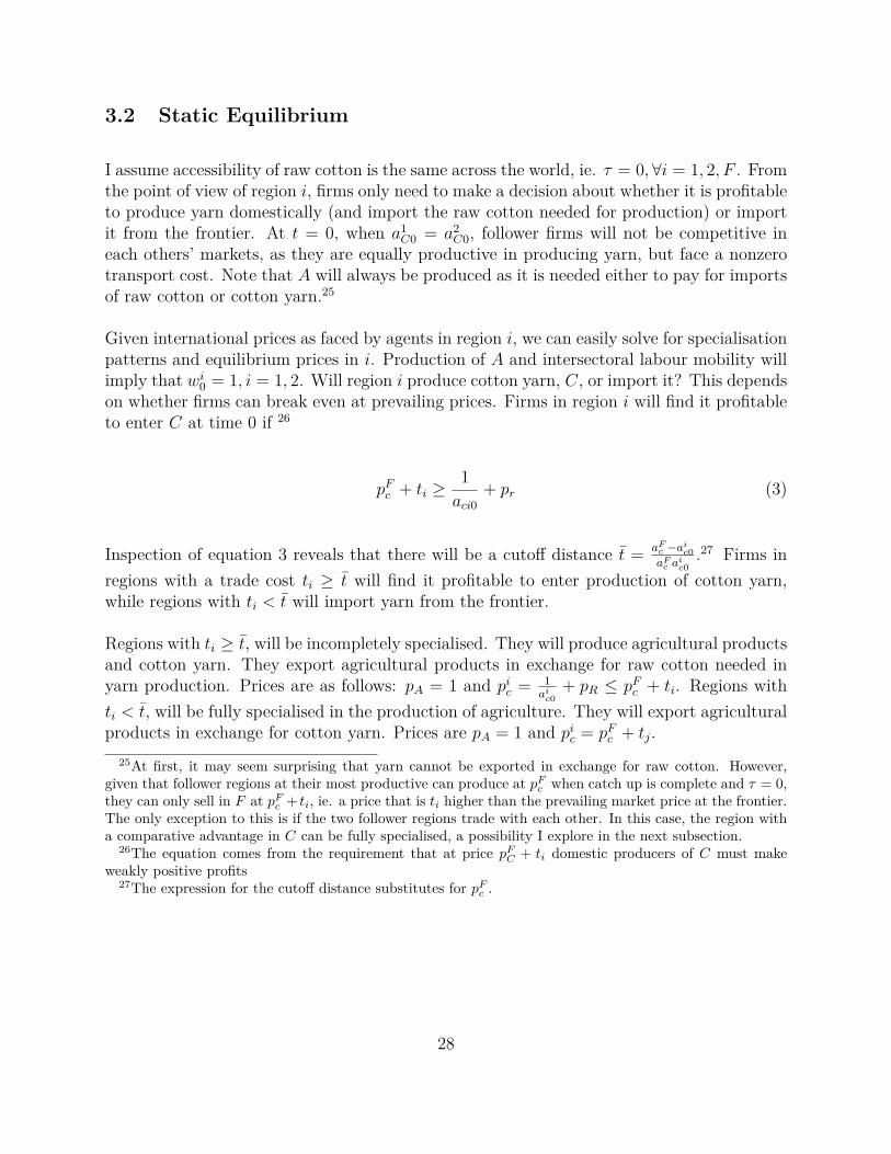
3.2 Static Equilibrium

I assume accessibility of raw cotton is the same across the world, ie. τ = 0,∀i = 1, 2, F . Fromthe point of view of region i, firms only need to make a decision about whether it is profitableto produce yarn domestically (and import the raw cotton needed for production) or importit from the frontier. At t = 0, when a1

C0 = a2C0, follower firms will not be competitive in

each others’ markets, as they are equally productive in producing yarn, but face a nonzerotransport cost. Note that A will always be produced as it is needed either to pay for importsof raw cotton or cotton yarn.25

Given international prices as faced by agents in region i, we can easily solve for specialisationpatterns and equilibrium prices in i. Production of A and intersectoral labour mobility willimply that wi0 = 1, i = 1, 2. Will region i produce cotton yarn, C, or import it? This dependson whether firms can break even at prevailing prices. Firms in region i will find it profitableto enter C at time 0 if 26

pFc + ti ≥1aci0

+ pr (3)

Inspection of equation 3 reveals that there will be a cutoff distance t = aFc −ai

c0aF

c aic0

.27 Firms inregions with a trade cost ti ≥ t will find it profitable to enter production of cotton yarn,while regions with ti < t will import yarn from the frontier.

Regions with ti ≥ t, will be incompletely specialised. They will produce agricultural productsand cotton yarn. They export agricultural products in exchange for raw cotton needed inyarn production. Prices are as follows: pA = 1 and pic = 1

aic0

+ pR ≤ pFc + ti. Regions withti < t, will be fully specialised in the production of agriculture. They will export agriculturalproducts in exchange for cotton yarn. Prices are pA = 1 and pic = pFc + tj.

25At first, it may seem surprising that yarn cannot be exported in exchange for raw cotton. However,given that follower regions at their most productive can produce at pF

c when catch up is complete and τ = 0,they can only sell in F at pF

c + ti, ie. a price that is ti higher than the prevailing market price at the frontier.The only exception to this is if the two follower regions trade with each other. In this case, the region witha comparative advantage in C can be fully specialised, a possibility I explore in the next subsection.

26The equation comes from the requirement that at price pFC + ti domestic producers of C must make

weakly positive profits27The expression for the cutoff distance substitutes for pF

c .

28

3.3 Dynamic Equilibrium

Given the static equilibrium from the previous section, characterising the dynamic pathof follower economies is straightforward. Regions which began producing cotton yarn attime 0 will increase their productivity in this sector via the production externality furtherstrengthening their competitive edge in the domestic market until aiCt = aFC and catch upis complete. Regions which import yarn from the frontier at time 0 will continue to importyarn and aiCt = aiC0, ie. productivity will stagnate at the initial level. The dynamic path isslightly more complicated if one region begins producing C at time 0, while the other doesnot. As productivity in the producing region increases, it becomes possible for the regionproducing C to become competitive in the region specialised in A. In this case, the twofollower regions will integrate. The economy with a comparative advantage in producing Cwill supply the other with cotton yarn in exchange for agriculture, while both are suppliedwith R from the frontier. Depending on the parameters, the following outcomes are thereforepossible:

1. If ti < t, i = 1, 2, both economies will specialise in the production of A and import C.˙aict

aict

= 0, ∀t and pict = pFc + ti.

2. If ti ≥ t, i = 1, 2, both economies will be incompletely specialised in producing A and Cfrom t = 0 onwards.

˙aict

aict> 0 and

˙pict

pict< 0 while aict < aFc . Once aict = aFc , pict = pFc ,∀t.

3. If ti ≥ t but tj < t and pFc + tj = 1ai

cT+ pr + tij, for some t = T then i will be incompletely

specialised in producing A and C and j will be fully specialised in producing A and importingC from the frontier while t < T . However, once t ≥ T , i will be competitive at exporting yarnto j. This will change the direction of trade and potentially alter specialisation patterns.Trade between the two regions will be as folllows: j is fully specialised in producing A, whichit exports to i in exchange for C.28

4. If ti ≥ t but tj < t and pFc + tj <1ai

ct+ pr + tij,∀t, i will be incompletely specialised in

producing A and C and j will be fully specialised in producing A and importing C from thefrontier. Labour productivity in producing C in i will never be high enough for firms to becompetitive in market j. This implies that i and j do not become integrated.

28Depending on parameters, i can be completely or incompletely specialised in producing C. It exports (orre-exports) A in exchange for R from the frontier. If pra

ict ≥ 1−2α, i is incompletely specialised in A and C.

However, for praict < 1−2α, i is fully specialised in C. As technology improves via the production externality,

complete specialisation becomes more difficult. This is the general equilibrium effect of C becoming cheaper.As C becomes cheaper, consumers in i and j increase consumption of C, but this requires more importsof R, which in turn increases demand for A. Supply of A can only be increased if i becomes incompletelyspecialised and this requires the wage to fall to one, where production in A is once again profitable.

29

A number of points are worth noting in light of this result. First, initial specialisation attime 0 will determine whether a domestic cotton yarn producing industry is able to developin a follower region i. This depends only on geographic distance to the frontier. Second,cotton yarn production is an infant industry in all follower regions. With sufficiently hightemporary protection from trade with the frontier in the production of yarn (ie. a sufficientlyhigh ti), all follower economies can develop their own cotton yarn producing sector whichis competitive with the frontier at any distance to the frontier. To see this, observe thatonce catch up is complete, acit = aFc , follower regions produce with the same technology asthe frontier. The extent to which this is welfare improving depends on the speed of learningrelative to discounting. If the industry is not competitive at initial distance to the frontier,ti, consumers are worse off during the time period where the cotton industry is protected,because they pay a higher price for cotton yarn than they otherwise would, but once thesector is competitive they are better off as the price of cotton yarn decreases below that ofcompeting imported yarn. The net effect thus depends on whether the long-term welfaregains outweigh the short term losses.

Finally, to the extent that one follower region is developing, while the other is not, thetime paths discussed in (3) and (4) differ only to the extent that under (3) the developingeconomy integrates with the stagnating economy, while in (4) it does not. The time pathdiscussed in (3) will prevail if productivity gains in C outweigh the trade cost tij between iand j. In particular, at 0, integration between i and j cannot take place, because i and jhave the same productivity, but i produces at a ti higher unit cost. As i produces in C, andaict increases, it can compensate for the higher trade cost, with higher productivity.

3.4 Understanding the trade shock

I now use this framework to guide empirical analysis. I build on the following two facts. (1)The shock to the price of yarn varied significantly across the French Empire. (2) The shockto raw cotton prices was fairly even across the French Empire. As the framework will makeclear, the two shocks together resulted in different changes in competitive pressure across theEmpire. The trade shock during the Napoleonic Wars effected cotton spinners’ incentives toproduce in two ways. First, the effective distance to Britain changed which effected tradecosts of British yarn ti. Second, the shock also drove up the price of raw cotton relative tothe price in Britain. Different to the price of yarn however, this shock was even across theFrench Empire.

In particular, let ∆ti ≡ t′i − ti denote the shock to trade costs for British yarn in region i,

where ti and t′i denote the trade costs between Britain and region i before and during the

Napoleonic Wars. Similarly, let ∆τ = τ denote the (common across regions) shock to theprice of raw cotton.

30

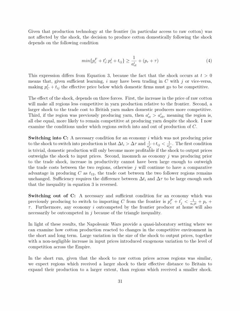
Given that production technology at the frontier (in particular access to raw cotton) wasnot affected by the shock, the decision to produce cotton domestically following the shockdepends on the following condition

min{pFc + t′i; pjc + tij} ≥1aict

+ (pr + τ) (4)

This expression differs from Equation 3, because the fact that the shock occurs at t > 0means that, given sufficient learning, i may have been trading in C with j or vice-versa,making pjC + tij the effective price below which domestic firms must go to be competitive.

The effect of the shock, depends on three forces. First, the increase in the price of raw cottonwill make all regions less competitive in yarn production relative to the frontier. Second, alarger shock to the trade cost to British yarn makes domestic producers more competitive.Third, if the region was previously producing yarn, then aict > aic0, meaning the region is,all else equal, more likely to remain competitive at producing yarn despite the shock. I nowexamine the conditions under which regions switch into and out of production of C.

Switching into C: A necessary condition for an economy i which was not producing priorto the shock to switch into production is that ∆ti > ∆τ and 1

ajct

+tij < 1ai

c0. The first condition

is trivial, domestic production will only become more profitable if the shock to output pricesoutweighs the shock to input prices. Second, insomuch as economy j was producing priorto the trade shock, increase in productivity cannot have been large enough to outweighthe trade costs between the two regions, otherwise j will continue to have a comparativeadvantage in producing C as t12, the trade cost between the two follower regions remainsunchanged. Sufficiency requires the difference between ∆ti and ∆τ to be large enough suchthat the inequality in equation 3 is reversed.

Switching out of C: A necessary and sufficient condition for an economy which waspreviously producing to switch to importing C from the frontier is pFc + t

′j <

1acjt

+ pr +τ . Furthermore, any economy i outcompeted by the frontier producer at home will alsonecessarily be outcompeted in j because of the triangle inequality.

In light of these results, the Napoleonic Wars provide a quasi-laboratory setting where wecan examine how cotton production reacted to changes in the competitive environment inthe short and long term. Large variation in the size of the shock to output prices, togetherwith a non-negligible increase in input prices introduced exogenous variation to the level ofcompetition across the Empire.

In the short run, given that the shock to raw cotton prices across regions was similar,we expect regions which received a larger shock to their effective distance to Britain toexpand their production to a larger extent, than regions which received a smaller shock.

31

Second, in the longer-term, if dynamic externalities of the type highlighted in this model areimportant, we expect regions which were able to scale up production to be more productivethan regions which remained more exposed to trade. For sufficiently large productivitydifferences, integration of the two economies as described in the third point of dynamicequilibrium is also possible. In the next two sections, I show that consistent with thesepredictions, department across the French Empire which received a larger trade shock (1)scaled up production to a larger extent than regions which received a smaller shock, and (2)in the longer run, these regions were not only more productive, but production became moreconcentrated in these areas.

4 Data

To analyse the question of how the rupture to trade relations effected the development ofmechanised spinning within the French Empire during the Napoleonic Wars, I collected datafrom two main sources. To understand changing trade routes, I extracted shipping data froma biweekly newspaper, the Lloyds List. To track regional development of mechanised cottonspinning, I collected handwritten departmental data from two different efforts of Napoleon’sinterior minsters to collect systematic statistical data on various branches of industry. Bothsources are described in more detail below. An example of the data is provided in Figures19 and 20 of Appendix C.

4.1 Shipping data

Data on trade routes was extracted using all editions of the Lloyd’s List between 1787-1814.The Lloyd’s List, one of the world’s oldest newspapers was set up by Lloyd’s Coffee House inLondon, which was a meeting point for underwriters of marine insurance at the time. Theunderwriters needed up to date news on shipping conditions, and for a small subscriptionfee Lloyd’s provided what was generally acknowledged to be the most up to date shippingbulletin of the time. Lloyd’s hired paid correspondents in each port to send information oneach ship that arrived to, or departed from a given port to the Post Master General withthe word “Lloyds” written in the corner. Each edition featured news on ships sailing fromand arriving to various ports. The coverage on arrival and departure of ships to all portsin Britain is believed to be a fairly reliable and representative source of information at thetime (Wright and Fayle, 1927).

Editions of the Lloyd’s List have been digitised by Google. To extract data from this source,I used an OCR programme to convert the images into machine-readable format and thenused a text-matching programme that searched for the names of European ports in the

32

Lloyd’s List. As port names have changed over time, and even within the time frame that Iexamine, numerous port names or spelling was in use for the same port, the names of portswere collected by manually searching through editions of Lloyd’s Lists. There are multiplesources of measurement error inherent in this procedure. First, the OCR and text-matchingprogramme introduce measurement error both in the form of matching mistakes and omittednames (the ones that could not be matched, or the European ports which I did not identify assuch). By comparing samples to the original, I found that incorrectly matched names wereminimal, and that the procedure picked up about 70-80% of the ports depending on thequality of the image. Finally, I also had one year (1808) manually entered in order to checkthat the sample with which I work is representative. There are around 3000 observations foreach year.

One potential problem with this data source is that during the blockade, parts of the Lloyd’sList were censored to protect smugglers and full information was only provided to insurersat the “Books and Notice Boards in the Subscribers’ Rooms” (Wright and Fayle, 1927). Itis precisely for this reason that a rival publication, The General Shipping and CommercialList was set up by post office clerks in 1808. Though the censoring will undoubtedly lead tomeasurement error in quantifying the trade routes, historians using different sources agreethat most smuggling was conducted using ports directly in the hands of the British, or portsallied to the British (Marzagalli, 1999 and Crouzet, 1964). This information did not need tobe censored. What needed to be censored was journeys that involved breaking Napoleon’sBerlin and Milan decrees (eg. direct shipping to French ports). Though smuggling of thisform undoubtedly took place, it does not seem to be quantitatively important. All evidencepoints to the fact that smuggling from ports relatively distant from the French Empire(eg. Malta or Sweden) were necessary, because direct smuggling was incredibly risky andexpensive (Crouzet, 1987). Finally, the Lloyd’s List was not censored in all Blockade years,and my findings for the uncensored years show similar results to censored years. Taking allforms of evidence together, censoring of the Lloyd’s List does not seem to be quantitativelyimportant as sources other than the Lloyd’s List corroborate my findings, a point to whichI return in section 5.

4.2 Cotton Data

Data on the cotton industry is observed at various points in time during the NapoleonicWars. Using this source, I have been able to construct a dataset which contains spindles atthe departmental level in 1803, 1806 and 1812. Data on all time periods is available for 88 ofthe 111 departments that formed a part of the French Empire in 1803 and 1812. The mostsystematic data collection was conducted in 1806 and then tri-yearly from 1810 onwards, butless systematic evidence is available in intermediate years too. Historians have described datafrom the Napoleonic Empire as the golden age of statistics, as the Imperial administrationwent to extensive efforts to collect systematic data on all branches of industry and society

33

(Gille, 1980). This remarkable effort means that firm level data is available for French cottonspinners at a very early stage of their development. To appreciate the importance of thisdata, it is worth noting that no similar data source is available in Britain for the 19th century.

Prefects in each department received four questionnaires in January 1806, one for each branchof the cotton industry; hosiery, mechanised spinning, weaving and printing.29 Regardingcotton spinning, firm level data was collected on the following: age of the firm, name ofthe entrepreneur, number of mechanised spinning machines, number of workers, output, andyarn count (measuring the finesse of the yarn produced) and source of raw cotton. Aroundhalf the firms also reported the number of spindles that each machine had. Using thisinformation together with the other firm level variables, I have imputed the average numberof spindles for the firms where this data is missing. By aggregating the firm level data up tothe departmental level, I have a measure of the number of spindles by department.

As one aim of the census was to evaluate how the industry had developed since the onsetof the war in 1803, the questionnaire also asked for the number of machines in 1803 whichcoincides with the British blockade the North Sea Coast. Using this information, I have alsobeen able to construct a measure of spindles at the departmental level in 1803.30

Data on spinning is only observed at the departmental level from 1810 onwards. Prefectswere asked to send tri-yearly reports on the state of various branches of industry in theirdepartments including cotton. I observe number of spindles, number of workers and output atthe departmental level. The reports were intended to inform the government in Paris aboutfluctuations in industrial activity. For this reason, there are sometimes large fluctuations inthe numbers reported. Furthermore, some prefects reported capacity while others reportedactive spindles. To gain the best possible measure of capacity, I utilise the reports in thefollowing way. In general, I take data from the year 1812 as this is the year closest to theend of the Blockade where data coverage is still sufficiently large.31 However, if the numberof spindles was larger in earlier reports (1810-11), I use these years. In the letters sent toParis, prefects usually indicate whether firms have gone bankrupt or whether they are idlefor cyclical reasons. I don’t use earlier numbers in instances where it is clear that activityin 1812 is lower because firms have gone bankrupt.

To conduct robustness to time-varying effects of geographic fundementals, I use data onmean-flows of rivers across France and proximity to coal, more details of which can be foundin Appendix C.

29Chassagne (1976) contains a detailed historical discussion on the census30Further details about the construction of the dataset are available from the author upon request.31As Napoleon’s power unraveled, and troops invaded the territory of France, fewer and fewer departments

submitted their reports.

34

5 Empirical Strategy

5.1 Empirical Framework

The rupture to trade routes caused by the Napoleonic Wars forced trade onto more circuitousand more expensive land-based routes. Variation in the extent to which trade routes acrossthe Empire were disrupted allows us to identify the effect of protection from British tradeon the development of mechanised cotton spinning. Higher trade costs increased the price ofcotton yarn at the destination. The shock to effective distance to Britain in any departmentis therefore a proxy for the shock to the price at which competing yarn entered a department.

The estimation strategy is based on a difference in difference strategy with continuous treat-ment intensity. Treatment is the distance shock which varies continuously across depart-ments. More formally, the outcome variable of interest, Sit, is a measure of the size ofmechanised spinning in region i at time t (spindles per capita in the baseline specification).The baseline specification estimates the following equation

Sit = αi + δt + γlnDit + εit (5)

where lnDit is a measure of effective distance to Britain in department i at time t. αi controlsfor time-invariant fixed effects at the departmental level, while δt controls for the effect ofaggregate shocks over time. dt is a dummy variable that switches on during the Blockade.γ is the parameter of interest measuring the effect of changes in effective distance to Britainon change in the number of spindles at the regional level.

The baseline specification estimates the equation in levels because of the large number ofzeros in the data, but I show that the results are robust to estimating the model as a Poissonconditional fixed effects regression. In baseline results, I divide by departmental populationto control for the fact that larger departments may increase spinning capacity by more thansmaller departments in response to the same shock simply because of their size, but resultsare similar when the equation is estimated in levels.

Identification using a difference in difference strategy relies on there being parallel pre-treatment trends prior to the Blockade. Furthermore, it also relies on there being no othershocks correlated with the distance shock at the time of the Blockade. To examine pre-treatment trends, I construct a measure of spinning capacity in the pre-treatment periodby using the age of firms from the 1806 census. To show that the distance shock is indeeddriving the differential development of mechanised cotton spinning, I examine two industrieswhere competition from Britain is less intense and technological change is not present at thetime, wool and leather. If the distance shock is driving the results, one would expect there

35

to be no effect on these industries. In the following, I also show that this is indeed the case.

5.2 Identification

5.2.1 Geographic Variation in the Effectiveness of the Blockade

Figure 8 documents (1) the geographic variation in the success of the Blockade outside of theFrench Empire, and (2) demonstrates that the Blockade was generally effective for regionswithin the French Empire.

In each panel of Figure 8, port level shipping data from the Lloyd’s List is aggregated upto the regional level so that the evolution of shipping over time can be examined. Datafrom 1787 onwards has been extracted in order to show that the Napoleonic Wars induced arupture to trade different to previous episodes such as the French Revolutionary Wars. Eachline represents a given region’s shipping with Britain as a share of total European shippingwith Britain. Panel A examines shipping to the Northern ports of Europe excluding portsthat belonged to the French Empire. I group ports into three groups: the North Sea coast,the Baltic and Scandinavia.

From the onset of the French Revolutionary Wars in 1793 until the peace of Amiens in 1802,there is a clear upward trend along the North Sea and Baltic. The Napoleonic Blockadediffers from other trade wars between Britain and France exactly because of the involvementof all European powers. Without neutral shipping to substitute for the loss of direct tradebetween Britain and France (as was the case during the French Revolutionary Wars), tradecosts became significantly larger. The fact that the North-Sea could not be used to substitutefor the loss of direct shipping between Britain and France is evident from the first grey linewhich shows the onset of the British blockade of the North Sea in 1803. The effect of theBritish blockade of the North Sea coast is to substitute to shipping via the Baltic. Between1803 and 1806, as shipping along the North Sea declined, the share of shipping to the Balticpicked up.

Accessibility of both the Baltic and the North-Sea worsened with the onset of the ContinentalBlockade in 1806 (denoted by the second grey line) as Prussia and Russia both implementedthe Blockade. It is during this time that Gothenburg became the important smuggling centrein the North, which can be seen by the increase in shipping to Scandinavia until around 1808.Marzagalli (1999) describes how merchants from Britain, Holland and Hamburg relocatedtheir business to Gothenburg to organise smuggling routes from this point. However, theproblem with Gothenburg was the lack of land connections to the German and Frenchregions, which were the final destination for most of these goods. Crouzet (1987) describeshow during a number of months in 1808 when the Blockade was fully effective both along

36

(a) British shipping with Northern Europe (b) British shipping with Southern Europe

(c) British shipping with France

Figure 8: British shipping with European regions as share of total, 1787-1814 (Lloyd’s List)

1 Notes: Figure 8 shows the time series of shipping between Britain and the given region as a share of totalEuropean shipping with Britain in order to understand regional variation in the effectiveness of theBlockade. For each year, the shares across the three subfigures add up to 1. The first grey line denotes theonset of the Napoleonic Wars in 1803, the second grey line indicates the onset of the Napoleonic Blockadein 1806 and they third grey line indicates the end of the Napoleonic Wars in 1813. See Appendix C fordata sources.

the North Sea and the Baltic, stocks piled up in Gothenburg as ships arriving from Swedenwere continuously denied entry.

It was possibly the increasingly difficult situation in the Baltic that encouraged merchantsto begin to lobby the British government for trading licenses to Heligoland. This tiny islandabout 50 kilometers off the German coast, measuring only a couple of square kilometers wastaken by the British navy in 1807. The intent was to track movements of the French armyalong the North Sea. The British government started granting licenses to merchants to trade

37

in Heligoland in late 1808, but smuggling began in earnest in 1809. The increase in the shareof shipping to the North Sea is accounted for single-handedly by this tiny island. Heligolandwas more advantageous as a smuggling centre for three reasons. First, it was closer to thefinal destination of the German and French markets reducing the land distances that goodswould need to travel. Second, small fishing boats could be used to smuggle goods onto alcovesand inlets on the North Sea coast during the night (Crouzet, 1987), something that had notbeen possible from Gothenburg. Third, the Baltic was only accessible by military convoy.To get to the Baltic, British ships needed to cross narrow straits controlled by the Danish,who had become Britain’s fiercest enemies as a result of Britain’s unprovoked bombardmentof Copenhagen in December, 1806.

Finally, it also clear that as the relationship between France and Russia deteriorated in thelead-up to Napoleon’s disastrous Russian campaign (1812) and Russian ports opened up toBritish shipping, trade through Sweden and the Baltic picked-up. For all of Heligoland’sadvantages, as constraints in the Baltic were loosened and ships could access Continentalports in the Baltic, trade was diverted away from Heligoland. This is suggestive of the factthat trade via Heligoland was costly, dangerous and expensive.

The situation in Southern Europe is far more clear-cut as is evident from Panel B whichshows the evolution of shipping for the Iberian Peninsula, the West- and East- Mediterranean.First, it is important to highlight the Iberian peninsula’s key importance in determining thefate of the Blockade. From the onset of the Blockade in 1806, this region’s share of shippingincreased dramatically. In fact, for two years, 60% of total European shipping with Britainwas conducted via the Iberian Peninsula. Gibraltar carried a large proportion of this trade,as did Lisbon and Cadiz, both of which were under British control from most of the Blockade.

The increase in shipping on the West-Mediterranean was driven almost single-handedly byMalta. Crouzet (1987) describes in detail the key importance played by Malta, especiallyin the smuggling of cotton goods. At one point, 8.8% of exports from Britain were takeninto Europe via Malta. The difficult, and often impossible situation in the North, drove theBritish to seek new markets, especially for cotton goods which were particularly dependenton export markets. One such market was the Mediterranean. Southern ports were usednot only as entry points for goods destined for French and German markets, but also asnew markets. Cotton goods in particular sought new markets on the Mediterranean. Aswas shown, Britain’s trade with the Mediterranean was not particularly important beforethe Blockade, but constraints in the North changed this. In some years, exports to theMediterranean surpassed pre-Blockade exports and Crouzet (1987) emphasises that cottongoods were the dominant export products in these markets.

Why was the Blockade so much less successful in these regions? To begin with, the Frenchnavy was in a weakened state on the Mediterranean as a result of an indiosyncratic politicalevent which took place during the French Revolution (Rogder, 2006). As Jacobite power was

38

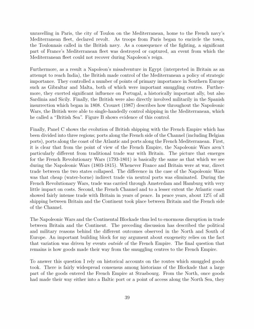
unravelling in Paris, the city of Toulon on the Mediterranean, home to the French navy’sMediterranean fleet, declared revolt. As troops from Paris began to encircle the town,the Toulonnais called in the British navy. As a consequence of the fighting, a significantpart of France’s Mediterranean fleet was destroyed or captured, an event from which theMediterranean fleet could not recover during Napoleon’s reign.

Furthermore, as a result a Napoleon’s misadventure in Egypt (interpreted in Britain as anattempt to reach India), the British made control of the Mediterranean a policy of strategicimportance. They controlled a number of points of primary importance in Southern Europesuch as Gibraltar and Malta, both of which were important smuggling centres. Further-more, they exerted significant influence on Portugal, a historically important ally, but alsoSardinia and Sicily. Finally, the British were also directly involved militarily in the Spanishinsurrection which began in 1808. Crouzet (1987) describes how throughout the NapoleonicWars, the British were able to single-handedly control shipping in the Mediterranean, whichhe called a “British Sea”. Figure B shows evidence of this control.

Finally, Panel C shows the evolution of British shipping with the French Empire which hasbeen divided into three regions; ports along the French side of the Channel (including Belgianports), ports along the coast of the Atlantic and ports along the French Mediterranean. First,it is clear that from the point of view of the French Empire, the Napoleonic Wars aren’tparticularly different from traditional trade war with Britain. The picture that emergesfor the French Revolutionary Wars (1793-1801) is basically the same as that which we seeduring the Napoleonic Wars (1803-1815). Whenever France and Britain were at war, directtrade between the two states collapsed. The difference in the case of the Napoleonic Warswas that cheap (water-borne) indirect trade via neutral ports was eliminated. During theFrench Revolutionary Wars, trade was carried through Amsterdam and Hamburg with verylittle impact on costs. Second, the French Channel and to a lesser extent the Atlantic coastshowed fairly intense trade with Britain in years of peace. In peace years, about 12% of allshipping between Britain and the Continent took place between Britain and the French sideof the Channel.

The Napoleonic Wars and the Continental Blockade thus led to enormous disruption in tradebetween Britain and the Continent. The preceding discussion has described the politicaland military reasons behind the different outcomes observed in the North and South ofEurope. An important building block for my argument about exogeneity relies on the factthat variation was driven by events outside of the French Empire. The final question thatremains is how goods made their way from the smuggling centres to the French Empire.

To answer this question I rely on historical accounts on the routes which smuggled goodstook. There is fairly widespread consensus among historians of the Blockade that a largepart of the goods entered the French Empire at Strasbourg. From the North, once goodshad made their way either into a Baltic port or a point of access along the North Sea, they

39

were transported overland to Strasbourg. Ellis (1981) estimates that up to 2/3 of importgoods made their way into the Empire through Strasbourg alone. This fraction underscoresthe enormous extent to which trade was disrupted and forced onto far more expensive landroutes during the Blockade. It is also a further piece of indirect evidence that direct smugglingbetween Britain and France could not have been quantitatively important as it would havesurely wiped out the far more circuitous route taken through Strasbourg. Ellis writes “ (...)smuggling was more active along the inland than the maritime frontiers of the Empire. Onereason for this was the nature of the terrain (...). Another was the proximity of foreignentrepots like Frankfrurt, Darmstadt, Mannheim, Heidelberg, Rastatt, Kehl and above allBasel. Within the Empire itself there were many smuggling bases up along the Swiss frontierand down the left-bank of the Rhine.” (Ellis, 1981, p. 203) 32

Figure 9: Traffic up-river and down-river from Strasbourg, Ellis (1981)

Regarding Southern smuggling, historians agree that many of the goods taken by the Britishto smuggling centres in the Mediterranean were destined for the French and German markets.There seems to have been a number of routes that the goods took. First, Livorno (part of theFrench Empire) seems to have been an important entry point for smuggled goods (Marzagalli,1999 and Galani, 2011). Second, Heckscher (1922) gives details of a smuggling route thatbegan from Trieste and brought goods up along the Danube into Germany and finally intoFrance. There is much less anecdotal evidence about smuggling through Spain, but thismay simply reflect the fact that shipping was relatively free throughout Spain and up to theFrench border there was no need bring goods via overland routes.33

32It may seem somewhat surprising that goods needed to be taken quite as far down South as Strasbourg.Why weren’t they smuggled into the Empire via the Kingdom of Holland, a much shorter route? TheKingdom of Holland proved to be far too permeable to the entry of British goods for Napoleon’s liking.While increasing pressure was placed on his brother, Louis, the King of Holland, to increase enforcementof the Blockade, the decision was made to close the Franco- Dutch border from 1808 effectively shuttingoff the potential entry of any smuggled British goods from the north (Heckscher (1922) p. 181.) For thisreason, British goods smuggled via the North took land routes all the way to Strasbourg prior to entry inthe Empire.

33One worry is that smuggling via the Iberian peninsula is overstated if the British also use the Iberian

40

Figure 9 shows the importance of the Rhine in the South-North trade. It is apparent thattrade downriver (South-North direction) significantly increases with the onset of the Block-ade. Ellis (1981) attributes this to the South-North smuggling. Goods entering the Continentfrom the South made their way to the Rhine via various routes and they were then shippedNorth along the Rhine.

5.2.2 Exogeneity

To what extent can we think of the blockade as captured by the distance shocks as exogenousto the mechanisation of the cotton industry? In particular, there may be a concern thatenforcement of the Blockade was systematically correlated with regions where the cottonindustry would benefit most from protection. There are two reasons why this is unlikely.First, as the previous section has documented, the fate of the Blockade was determinedmostly by events outside of the French Empire and outside of Napoleon’s direct control. Itwas not that Napoleon did not want to implement the Blockade in the South to the sameextent as in the North, it was that he could not. Second, Napoleon’s primary aim wasto defeat Britain. As was documented, the cotton industry’s reliance on imported inputsmeant that Napoleon was decidedly ambivalent about the positive developments in the cottonindustry as it meant relying on colonial products.

5.2.3 Quantifying the Distance Shock

To quantify the distance shock I use two approaches. As any measure is likely to suffer frommeasurement error, I construct two separate measures of the Blockade and check the extentto which results change if one is used as an instrument for the other.

1. Measure 1: Cost-DistanceThe first measure uses a shortest route algorithm to calculate the distance betweenLondon and the prefecture of any department. I account for one of the most importantdrivers of increasing trade costs - the difference between water- and land-borne routes,by calibrating the ratio of the two to match the fact that at this period in time sailingfrom Rouen to Marseille was 2/3 the cost of going overland (Daudin, 2010). Using this

peninsula as a point of access to markets in Latin America. Crouzet (1987) discusses the trade from Britain toSpanish and Portuguese colonies in detail. He finds that in fact, because of the weakened state of the Spanishand Portuguese monarchy, the British actually had direct access to these markets in contrast to the periodbefore the Blockade when British goods could only enter the markets in Latin America indirectly via eitherSpain and Portugal or smuggling via free-ports in the Carribean. This implies that if anything, comparingshipping between Britain and the Iberian peninsula before and during the Blockade will understate theextent to which the peninsula was used for smuggling.

41

evidence, 1 sea kilometre is equivalent to about 0.15 kilometres on land. Pre-Blockadedistance is calculated as the direct shortest route between London and the capital ofany department. Any port that was in use between 1787-1814 (the years for whichshipping data has been extracted) can be used to reach the capital of any department.To calculate the shortest route between London and the capital of the departmentduring the Blockade, I use historical accounts for smuggling routes. In particular, Itake Malta, Gibraltar, Gothenburg and Heligoland as the smuggling centres to whichgoods arrived from London. To make it to France, these goods could either take theNorthern overland smuggling route via Strasbourg discussed in the previous section,or a Southern smuggling route via Trieste or Livorno, two documented smugglingcentres,34 or via Bilbao and Barcelona. As was mentioned in previous sections, wehave less information on smuggling via Spain, so I have taken two ports, Bilbao andBarcelona on the Atlantic and Mediterranean as routes from which goods could enterthe French Empire. Figure 14 in Appendix B gives an example of how the shortestsmuggling route is calculated for one department.For any department i, the algorithm then picks the shortest route. The shock, bydepartment, can be seen in Figure ??, where darker coloured circles show a largerlog-distance shock. As expected, departments along the Channel have the highestcost-distance shock. However, the shock worked in a more complicated way thansimply increasing from South to North. For example, the departments along the Rhinewitnessed almost no increase in their effective distance to London by virtue of theirproximity to Strasbourg, the route via which goods entered the department. The routesthat goods took prior to the Blockade were almost identical to the routes which theytook during the Blockade. In contrast, the Atlantic seaboard witnessed a much largerincrease in trade costs, as these departments initially had relatively cheap access viasea-routes, which were not available during the Blockade.

2. Measure 2: Weighted DistanceThe main source of measurement error in the cost-distance shock stems from the factthat it does not account for capacity constraints and periods where smuggling centreswere not open. As I have shown, military events played a role in which areas ofthe Continent were more or less were open to trade and this variation has a timedimension to it. For example, in years where the Blockade in the North was almostperfectly enforced, goods made their way into Continental Europe exclusively via theSouth. The second measure therefore focuses on capturing the intensity of use of anysmuggling centre between 1803-12 instead of the shortest route approach.To capture the intensity of port-usage, I use the Lloyd’s List to identify ports that wereintensively used during the Blockade. A smuggling centre is defined as a port wherethe number of ships sailing to or from Britain and the given port in any of the Blockadeyears between 1803-1812 was greater than the amount of ships in any of the years before

34On the smuggling centres, see Crouzet (1987) and Marzagalli(1999).

42

(a) Effective distance to London shock (Mea-sure 1)

(b) Effective distance to London shock (Mea-sure 2)

1 Notes: Measure 1 uses a shortest route algorithm to calculate the log-distance between the prefecture ofthe department and London before and during the Blockade. Measure 2 calculates the distance shock inthe following way. Pre-blockade distance is simple Euclidean distance to London. Distance to Britainduring the Blockade is calculated as the weighted Euclidean distance between Britain and smugglingcentres. Smuggling centres are identified as ports where shipping during the Blockade increasessignificantly, and weights are the share of a given smuggling centre in total smuggling. The log-differencebetween the two gives the shock. See text for details.

the onset of the Blockade for which we have data (1787-1802). I use this conditionin order to avoid mis-classifying ports which happen to be open to trade with Britainbut are not used as smuggling centres. This is a strict condition because shipping toEurope in general decreases quite significantly, so any port that shows an increase itabsolute numbers, should play a role in the new commercial routes. To focus on thequantitatively important smuggling centres, I further refine this measure by using onlythe ports where the maximum yearly shipment in a Blockade year exceeds 80. Thelarge and important smuggling centres such as Malta have above 300 shipments in peakyearsBased on these conditions, the quantitatively important smuggling centres are: Cadiz,Corunna, Gothenburg, Gibraltar, Heligoland, Lisbon, Malta and Tonningen (whichwas used between 1803-05). These ports (with the exception of Corunna, whose shareis below 2%) all play a prominent role in the historical literature as smuggling centresfor British goods as was discussed in previous sections.35

The final step is to quantify the relative importance of each centre. To do this, I havetaken total shipments between 1803-1812, the Blockade years, and subtracted totalshipments between 1793-1802. The difference between the two is a crude measure of

35Cadiz, close to Gibrlatar, played a role similar to Gibraltar as it was under British control for most ofthese years.

43

smuggling. Weights are calculated based on a port’s share of total smuggling. Ship-ments to the Southern smuggling centres account for roughly 70% of total smuggling.Pre-Blockade distance according to this measure is proxied by Euclidean distance toLondon, while distance during the Blockade is given as a weighted average of the Eu-clidean distance to each smuggling centre. I measure distances in this way to capturethe idea that supply in the North (ie. Heligoland, Gothenburg and Toning) is plausiblybelow demand and part of North’s demand is satisfied via shipments from the South.Note that by calculating distances in this way, I am being conservative with estimatesof the distance shock in the sense that while there is evidence for trade flowing in theSouth-North direction, (eg. from Malta to the Northern parts of Europe) there is nohistorical account of trade flowing in the North - South direction (eg. from Heligolandto Southern Europe). This makes sense, seeing as the binding supply constraint seemsto be in the North and not in the South. In this way, this measure is probably over-estimating the South’s distance shock relative to the North stacking the cards againstfinding an effect of distance on capacity. Though calculated using a different approach,the two measures of the shock are highly correlated (correlation: 0.88)

6 Results

6.1 Baseline Results

Table 2 contains the results from estimating equation 5. The dependent variable in allcolumns is spindles per thousand inhabitants. The distance measure used is the cost-distanceshock (measure 1). The estimated coefficient is large, and statistically different from zeroacross all specifications. The point estimate of 32.72 in column (3) implies that movingfrom the 25th to the 75th percentile of the distance shock leads to a predicted increase inspinning capacity per capita that is slightly smaller in size than the mean per capita spinningcapacity across departments at the end of the Blockade. Standard errors are clustered atthe departmental level, as Conley’s standrd errors tend to generally give a smaller standarderror.

Columns (1) - (3) add time and departmental fixed effects one at a time. Comparing Columns(2) and (3) reveals that adding the departmental fixed effects has a relatively small effecton the point estimate and the standard error (35.64 and 32.72). Correlation between thedistance shock and relevant unobservables fixed over time at the departmental level seemsto be small. Nonetheless, it may be the case that some geographic variables such as accessto fast flowing streams, or coal have a time-varying effect. For example, as mechanisationin cotton spinning developed, water and steam-powered machines became more prevalent.Therefore, these “geographic fundamentals” may have time-varying effects.

44

Column (4) shows that adding access to fast-flowing rivers and coal interacted with the time-dummy has practically no effect on our coefficient of interest. Both variables are constructedsuch that a higher number means better access.36 Figure 18 in Appenidx B shows that,unsurprisingly, the mountainous regions around Lyon had far better access to fast flowingstreams than the flatter Northern plains, and both had relatively similar access to coal.

One concern may be that the institutional change brought about by the French Revolu-tion affected departments differently. If the effect of institutional change is correlated withthe distance shock, the estimated coefficient will be plagued by the effects of institutionalchange.37 The most obvious way in which institutional change could differentially affectdepartments is through territorial expansion. Regions were annexed to the French Empireat different points in time during the French Revolutionary and the Napoleonic Wars. Theseregions were therefore also effected by institutional change later than departments of “ancienregime” France. To assess the extent to which institutional change is a concern for our speci-fication, Column (5) restricts the sample to areas which formed part of France prior to 1789.These departments were all effected simultaneously by the French Revolution, therefore theeffect of institutional change should arguably be more even within these departments. Theestimated coefficient remains significant and the point estimate increases somewhat in size(from 32.9 to 39.38).

Column (6) instruments the cost-distance measure using the second measure of distance.Consistent with endogeneity resulting from measurement error, the point estimate increasesin size by about 20% with a marginal improvement in precision. Finally, calculating distancefrom London may not be a good approximation to the distance shock, if cotton was exportedpredominantly from other ports. Crouzet (1987) identifies London and Liverpool as the maincenters from which cotton was exported. For this reason, Column (7) calculates the distanceshock using Liverpool as the source port in Britain instead of London. Again, the estimatedcoefficient is somewhat larger (37.54), but similar in magnitude.

36Access to coal is measured as the log of the inverse of the minimum distance (multiplied by 10,000) toa major European coal-field following Fernihough and O’Rourke (2014), while access to fast flowing streamsis the log of the departmental average across rivers of the mean monthly flow rates in each department. SeeAppendix C for sources.

37Acemoglu et al (2009) examine the effects of institutional change brought about by the French Revolutionin German states.

45

Table 2

Baseline Specification

Spindles per thous inhabs (1) (2) (3) (4) (5) (6) (7)

Distance shock (Lo) 25.72*** 35.64*** 32.72*** 32.90*** 40.15*** 38.95***(7.15) (12.03) (10.10) (10.33) (9.608) (12.86)

Distance shock (Li) 37.54***(12.74)

Rivers*Time 0.66 0.60 0.61 0.31(1.18) (1.40) (1.25) (1.19)

Coal*Time -2.26 2.52 -2.54 -1.56(3.33) (5.52) (3.32) (3.79)

Time FE No Yes Yes Yes Yes Yes YesDeptartmental FE No No Yes Yes Yes Yes YesObservations 176 176 176 176 142 176 176R-squared 0.158 0.177 0.363 0.365 0.375 0.305Number of dept 88 88 88 88 71 88 88

Notes: Depvar is spindles per thousand inhabitants, Col (1) - (4) estimate the baseline specification adding time anddepartmental fixed effect, and a control for the time-varying effect of access to fast-flowing streams and coal, Col (5)restricts the sample to “ancien regime” France, Col (6) instruments the cost-distance shock with the weighted distanceshock, Col (7) uses cost-distance shock measured from Liverpool as opposed to London. Standard errors are clustered atthe departmental level to account for serial correlation, *** p<0.01, ** p<0.05, * p<0.1

6.2 Robustness

6.2.1 Falsification test using woollens and leather

Identification relies on there being no other shocks contemporaneous to and correlated withthe distance shock. To show that the shock is indeed identifying the effect of protection fromBritish trade, Table 3 shows that the effect which I find for cotton spinning is not present fortwo other industries, wool yarn (a substitute) and leather. Both products are less intensivelytraded with Britain, and there is no technological change either. For these reasons, the shockshould not have a significant effect on the spatial distribution of activity in these industries.

At the turn of the 19th century, both industries were still very much organised as rural,cottage industries in contrast to cotton spinning. Mechanisation had not been introduced inthe woollen industry because of inherent differences in the fibre which made mechanisationof wool spinning more difficult (Landes, 1969). For this reason, in woollen spinning, thedependent variable cannot be anything but labour employed. As I argued previously, woolwas not an intensively traded good with the British, and the raw material was also pre-dominantly domestically supplied. Finally, it was an entrenched industry which enjoyed a

46

high level of state support. For example, the army used exclusively woollen products (Boninand Langlois, 1997). The caveat with using wool spinning is that there may be spilloversfrom the cotton industry. It is conceivable that in the areas where cotton spinning becamewidespread, wool spinning was squeezed out.

For this reason, I also collected data on the leather industry. Leather was similarly rurallyorganised, with some military demand during the period and no significant technologicalimprovement. More than either woollens or cotton, it mostly served local markets and usedlocal supply with access to water being the one locational constraint making it an idealindustry with which to contrast cotton spinning (Bonin et Langlois, 1997).

There are three further considerations which should be taken into account when interpretingthe results. First, in the case of both industries, the pre-Blockade data point comes fromindustrial surveys carried out directly after the French Revolution in 1789. Second, in bothcases, the data from the pre-Napoleonic period are generally worse quality simply becausethe questionnaires were more qualitative in nature. Third, because in this case the firstdatapoint is in the 1790s (before France’s territorial expansion), the sample is restricted tothe territory of “ancien regime” France.

Table 3: Falsification test: Woollen spinning and leather production

Leather Industry Wool Industry

(1) (2) (3) (4) (5) (6)Activity per thous inhabs FE IV FE FE IV FE

ln Distance shock (Lo) 0.397 0.468 -4.625 -4.653(0.287) (0.312) (4.563) (4.620)

ln Distance shock (Li) 0.410 -5.613(0.300) (5.827)

Time FE Yes Yes Yes Yes Yes YesDept FE Yes Yes Yes Yes Yes YesObservations 124 124 124 138 138 138R-squared 0.064 0.062 0.046 0.210 0.210 0.205Number of dept 62 62 62 69 69 69Notes: Depvar in woollen spinning is employment per thousand inhabitants, in leather it is numberof pits per thousand inhabitants, Cols (1) and (4) estimate the baseline specification includingdepartmental and time fixed effects, Cols (2) and (4) instrument the cost distance shock usingthe weighted distance shock, Cols (3) and (6) estimate the effect of the shock using distance fromLiverpool instead of London, Standard errors are clustered at the departmental level to account forserial correlation, *** p<0.01, ** p<0.05, * p<0.1

47

Figures 15 and 16 in Appendix B show scatterplots for changes in production capacity plottedagainst the distance shock for both wool and leather. Columns (1) - (3) in Table 3 replicatethe baseline estimation from Table 2 for production capacity in leather (number of pits),Columns (4) - (6) replicate the same for employment in woollen spinning. Columns (1) and(4) give the baseline fixed effects estimate, Columns (2) and (5) use the second distancemeasure as an instrument for the first, while Columns (3) and (6) use the source port asLiverpool instead of London. The estimated coefficient is not significant at standard levelsin any of the specifications. The size of the estimated coefficient in the leather industry fromColumns (1) - (3) is not small however. Moving from the 25th to the 75th percentile of theshock leads to an increase in predicted pits which is about 60% of the mean number of pitsafter the Blockade. Closer examination of the results reveals however, that this is drivenentirely by two extreme outliers (Var and Ardennes, see Figure 16). Dropping these reducesthe estimated coefficient from 0.397 (se 0.287) to 0.011 (se 0.115) which is essentially a zeroeffect.

The negative coefficient for woollens seems to suggest that a spillover effect from cotton towoollen spinning may be present, though it cannot be precisely estimated. Moving fromthe 25th to the 75th percentile of the shock leads to a predicted decrease in employment inwoollen spinning per thousand inhabitants that is 60% of the mean spinning employmentat the end of the Blockade, though the estimated coefficient is not statistically significantacross specifications. The estimated coefficient is also less sensitive to dropping outliers.Repeating the same exercise of dropping the two departments where the change was thelargest in absolute value (Lozere and Ardennes) decreases the magnitude of the estimatedcoefficient in Column (4) from -4.625 (se 4.563) to -1.980 (se 1.891).

6.2.2 No pre-treatment trend

One concern may be that the effect which is attributed to the trade shock would have takenplace independently of the Napoleonic Wars. If technology flows are correlated with distance,areas closer to Britain (ie. departments along the English Channel) should have acquiredan advantage over regions further away. This is one mechanism via which the assumption ofparralell pre-treatment trends may be violated. To show that this mechanism is not drivingmy results, Table 6 in Appendix A shows that the development of mechanised spinningacross the French Empire prior to 1803 was not systematically related to the shock. In theabsence of similar data for this period, I have constructed an approximation to spindles in1794 using firm level data from 1806. I take spinning capacity in 1803 for firms alive in 1794as an approximation to actual spinning capacity at the departmental level in 1794, whichI don’t observe. Of course, this assumes that all growth in spinning capacity took placeon the extensive margin and that firms didn’t go bankrupt. Both are strong assumptions,though for this placebo test to be valid, we only need to make the weaker assumption thatbankruptcies and adjustment in spinning capacity at the firm-level between 1794-1803 were

48

not systematically related to the shock.

The period 1794-1803 is chosen as this time horizon is the same as the treatment periodmaking the estimated coefficient between the two periods comparable. Furthermore, thisis also when the Reign of Terror ended in France. The estimated coefficient for the period1794-1803 is not only not significant at conventional levels, but the point estimate is also1/16-th the size of the point estimate for the treatment effect (2.78 vs 32.72).

6.2.3 Factor price shocks

Another concern is that the Napoleonic Wars may have effected relative factor prices alteringthe profitability of mechanising the production process. For example, it is widely believedthat conscription caused a negative labour supply shock driving up wages. If wages increasedrelative to the cost of capital disproportionately in areas which received a larger shock, thiswould bias the estimated coefficient upwards. To show that this is unlikely to be the case, Iexamined the capital to labour ratio in mechanised spinning across departments in 1812. Ifthere was a disproportionate increase in the wages relative to the cost of capital it should besystematically related to the capital labour ratio as the two are substitutable. Figure 17 inAppendix B shows that there is no systematic relationship between the capital labour ratioand the distance shock.

6.2.4 Specification Issues

Tables 7 - 8 in Appendix A contain further robustness checks related to specification issues.First, departmental population is available for the majority of departments only in 1811. Thisis problematic if departmental population changed in response to the shock. For this reason,I replicate the specifications in Table 2 using the level of spindles as the dependent variable.The estimated coefficients in Table 7 show a broadly similar picture. The magnitude ofthe coefficient is somewhat larger, as moving from the 25th to the 75th percentile leads toa predicted increase in spindles which is larger than the mean number of spindles acrossdepartments in 1812. This makes sense as the area around Paris has a few departmentswhich were both fairly large and increased their spinning capacity during the NapoleonicWars. Their effect is dampened in the per-capita estimates.

Second, as noted, the baseline specification is estimated in spindles per capita because of thelarge number of zeros in the sample (around 1/3 of the departments have zero spindles ineither 1803 or 1812). These departments usually have a small number of spindles to beginwith and decline to zero in 1812, or they start with zero spindles in 1803 and increase to asmall number. Some of this is plausibly measurement error. Very small, rural firms may or

49

may not show up in the estimates in a given year. Furthermore, the economic significance ofmoving from zero to a small number or vice-versa is small relative to the magnitudes involvedwith some of the departments who increase spinning capacity significantly. Estimating thespecification in logs or with a Poisson specification, will attribute a very high growth rate tothe former observations, while departments that started with a modest number of spindlesand grew to be important spinning centres will have higher a growth rate. For example,the department Aisne grew from having around 1,400 spindles in 1803 (not more than acouple of machines) to over 60,000 in 1812. Contrast the economic significance of this toHaute-Saone, which increased its spinning capacity from 0 to 840.

Nevertheless, I show in Table 8 that using a Poisson specification in levels or in per capitaterms leads to a positive and significant coefficient (though when estimated in levels, thecoefficient is significant only at 10%). The estimated elasticity is between 0.4 and 0.7.Dividing by departmental population will dampen the effect that small departments movingfrom 0 to a few hundred spindles will have. Indeed, when estimated in per-capita terms, thepoint estimate increases both in precision and in size.

Appendix A also shows that results are robust to allowing for spatial correlation across de-partments in the error terms and it also gives details on a more flexible specification. Finally,the results on cotton spinning are robust to dropping departments from the specification oneat a time.

7 Long Term Effects

The previous section demonstrated that the trade shock induced by the Napoleonic Warsled to a disproportionate increase in spinning capacity in the departments that were betterprotected from trade with the British. Up to this point, the evidence presented is consistentwith inefficient French firms scaling up their production during a period in which they enjoyprotection from British competition. This section presents three facts that rule out thishypothesis and are consistent with the predictions of the learning-model.

1. French exports of cotton goods increased after 1815Panel A and B of Figure show the evolution of French exports of cotton goods in levelsand relative to British exports of the same. French exports initially declined as theNapoleonic Wars drew to a close. The decrease in exports prior to the fall of Napoleoncan be explained by a number of events. First, from 1813 onwards military activity wastaking place within the borders of the French Empire and prefectural reports from thisperiod indicate that some cotton mills were inactive for this reason. Second, the bordersof France were redrawn at the Congress of Vienna in 1815. Important cotton spinning

50

regions in present-day Belgium were detached from the Empire. Third, as Britishexports to the Continent could again take the the cheaper, direct routes, competitionin exports markets and in France became higher.38

Following this initial dip however, exports of cotton goods increased continuously,providing evidence that French firms were able to compete at world market pricesafter peace to the Continent was restored. Furthermore, Panel B shows evidence ofmodest catch-up vis-a-vis Britain. French exports of cotton goods grew faster over thistime period than British exports.

(a) French exports of cotton, Fr (b) French vs British cotton exports

1 Notes: Panel A displays the time series of French exports of cotton goods in francs during and after theNapoleonic Wars. Panel B shows the same as a ratio of Britain’s exports of the same. See Appendix C fordata sources.

2. Emulation of Britain’s success in cotton was difficultFigure 12 shows evidence that contradicts the idea that slow-technological diffusionmeant that, with time, Continental European countries would inevitably follow Britain’spath to industrialisation. Even as late as 1851, at the time of the Chrytsal Palace Ex-position in London, Britain’s absolute dominance in industry in general, and cotton inparticular was evident (Landes, 1969). In cotton spinning, there were two countries,France and Belgium - both part of the French Empire up to 1815, that outperformedthe rest of Continental Europe in terms of cotton spinning.Figure 12 follows the evolution of raw cotton consumption per capita for various Conti-nental European countries between 1830-50. Raw cotton is a proxy for cotton spinningas this is the primary (imported) input used in production. The size of the industry

38French producers faced domestic competition only for a short period of time as the government soonplaced a non-tarrif barrier on imports of cotton goods (O’Rourke and Williamson, 1999)

51

across Europe in 1850, over 30 years after the end of the Blockade was significantlysmaller in all other countries. Note in particular, that Sweden, Britain’s most con-sistent ally throughout the Napoleonic Wars and a key smuggling centre for Britishproducts, had no cotton spinning to speak of even in 1850. Note also the time seriesfor the Dutch, as well placed by their proximity to Britain as Belgium and Northern-France to benefit from technology flows, but less well protected during the NapoleonicWars. The Dutch and Belgian regions were in fact one country between 1815-1830 giv-ing them an even closer source for technology adoption after 1815. With institutionsthat rivalled Britain’s, they are as close to an ideal counterfactual as one could hope.The fact that they have a very small cotton industry according to the data and in linewith other historical evidence (Mokyr, 1976), is strongly suggestive evidence againstboth the claim that emulation was inevitable, and the claim that it was related todistance to Britain.

Figure 12: Raw cotton consumption per capita (Mitchell, 2007)

3. Areas within France which received a higher trade were more productive cotton spinnersin 1840Data from the first French industrial census of firms conducted between 1839-47 pro-vides information on the spatial distribution of spinning activity.39 Figure 13 showsthe spatial distribution of cotton spinning employment across departments. The figure

39The data was digitised by Chanut et al (2000).

52

Figure 13: Employment in cotton spinning, 1839-41 (Source, Chanut et al., 2000)

makes clear that the concentration of industry in the North and North-East becamemore pronounced over time. A learning externality would imply that with time, firmsthat are located in areas which received a larger trade shock become more productiveas they moved down their industry-wide cost curve. Table 4 shows evidence consistentwith this prediction. In these regressions, I examine whether labour productivity at thefirm level is associated with the distance shock. In particular, I estimate the followingequation.

Ai = α + βTi + γ′Xi + εi (6)

Ai is the log of sales per employee for firm i, Ti is the log-distance shock and X isa matrix of controls. The results of this estimation are presented in Table 4. Theelasticity of productivity with respect to the trade shock enters with a positive andsignificant coefficient across specifications. A one standard deviation increase in theshock leads to a 20-40% standard deviation increase in the predicted log-(productivity).The results are robust to introducing both firm level (firm size, source of power, share ofchildren and female employed) and departmental (population and total sales) controls.Furthermore, the results are robust to trimming the top and bottom 1% of the data(in terms of productivity) to remove the largest outliers.Taking these facts together makes a strong case for the claim that temporary protectionfrom trade with the British in parts of the French Empire led to the development of amodern cotton spinning sector that was viable in the long term.

53

Table 4: Long term effect on within country spinning productivity

Full Sample Trimmed (Top-Bottom 1%)

(1) (2) (3) (4) (5) (6)Sales per Employee (1840)

Distance shock (Lo) 0.105*** 0.128*** 0.205*** 0.131*** 0.143*** 0.216***(0.0288) (0.0191) (0.0343) (0.0281) (0.0187) (0.0303)

Firm Size 0.275*** 0.276*** 0.196*** 0.209***(0.0518) (0.0470) (0.0287) (0.0282)

Share children -0.649** -0.680** -0.515* -0.569**(0.292) (0.268) (0.297) (0.276)

Share women -0.640** -0.692*** -0.493* -0.550**(0.262) (0.246) (0.256) (0.248)

Water power -0.0734 -0.0933 -0.0230 -0.0506(0.0885) (0.0788) (0.0810) (0.0708)

Steam power -0.275*** -0.231*** -0.195*** -0.147***(0.0511) (0.0437) (0.0605) (0.0478)

Population 1801 -0.301*** -0.363***(0.100) (0.0980)

Spinning Activity 0.00456 0.0280*(0.0178) (0.0155)

Observations 531 530 530 520 520 520Number of clusters 43 43 43 40 40 40R-squared 0.043 0.287 0.300 0.098 0.264 0.292Notes: Depvar is the log of sales per employee, Firm size is proxied for by the log of primary material used (value),

Share women and Share children is the share of the respective category in total employment (excluded is men),Water power and Steam power are binary indicators for power source employed, Pop 1801 is the log of departmentalpopulation in 1801, Spinning activity is the log of total sales in cotton spinning in the department excluding thegiven firm, Standard errors clustered at the departmental level to account for within group correlation,*** p<0.01,** p<0.05, * p<0.1

8 Conclusion

This paper has documented a sequence of events which suggests that in some settings,infant industries can benefit from temporary protection from trade. The preceding argumenthas demonstrated that starting from similar initial conditions, the invention of mechanisedspinning in Britain led to enormous gains in productivity. Continental Europe did not followBritain’s lead. Mechanisation in France prior to the Blockade proceeded slowly. The priceof both yarn and capital (spinning jennies) was higher in France rendering French producersuncompetitive.

54

The trade shock caused by the Napoleonic Wars led to plausibly exogenous variation in theextent to which trade routes between the French Empire and departments were affected.The paper has shown that regions which received a larger shock were also the ones whichscaled up production in mechanised cotton spinning to a larger extent. Temporary protectionproved to have persistent effects. French exports of cotton goods increased after 1815 relativeto British exports of the same. We do not find similar increases in production capacity inareas of Continental Europe outside the French Empire. Finally, French producers were notonly more numerous in the North in 1840, they were also more productive.

The external validity of this particular setting is of course questionable. What can developingcountries hoping to expand their manufacturing sectors today learn? There are two aspectsto this question. On the one hand, the technological gap between 19th century Britain andFrance was far smaller than the technological gap between the richest and poorest countriestoday. On the other hand, technology flows, in some settings, could arguably be faster asa result of better access to information and lower barriers to the exports of machines andlabour. To strengthen external validity, future research should focus on gaining a betterunderstanding of the precise mechanisms at work in order to distinguish contexts in whichthe economic mechanisms underling infant industry work, and also the cases in which theydon’t.

55

9 References

Acemoglu, D., Cantoni, D., Johnson, S., Robinson, J. A. (2009). The consequences of radicalreform: The French Revolution (No. w14831). National Bureau of Economic Research

Amsden, A. H. (2001). The rise of “the rest”: challenges to the west from late-industrializingeconomies. Oxford University Press

Allen, R. C. (2009). The British Industrial Revolution in Global Perspective. CambridgeUniversity Press.

Aspin, C., Chapman, S. D. (1964). James Hargreaves and the Spinning Jenny. Preston:Helmshore Local History Society.

Bonin, S., Langlois, C. (1997). Atlas de la Révolution française: Economie (Vol. 10).Editions de l’Ecole des hautes études en sciences sociales

Broadberry, S., Gupta, B. (2009). Lancashire, India, and shifting competitive advantagein cotton textiles, 1700–1850: the neglected role of factor prices1. The Economic HistoryReview, 62(2), 279-305.

Chabert, A., Lefebvre, G. (1949). Essai sur les mouvements des revenus et de l’activitééconomique en France de 1798 à 1820. Librairie de Médicis

Chanut, Jean-Marie, Jean Heffer, Jacques Mairesse, Gilles Postel-Vinay, Frédéric Boccara,Pierre Sicsic, André Straus, and Patrick Verley. "L’industrie française au milieu du 19 esiècle(les enquêtes de la statistique générale en France)." Recherches d’histoire et de sciencessociales (2000).

Chapman, S. D. (1970). Fixed Capital Formation in the British Cotton Industry, 1770–18151.The Economic History Review, 23(2), 235-253.

Chapman, S. D. Chassagne, S. (1981): European Textile Printers in the Eighteenth Century:A study of Peel and Oberkampf, Heinemann Educational Books, London

Chassagne, S. (1976). L’Enquête, dite de Champagny, sur la situation de l’industrie coton-nière française au début de l’Empire (1805-1806)’. Revue d’histoire économique et sociale,54, 336-370.

Clemens, M. A., Williamson, J. G. (2001). A tariff-growth paradox? Protection’s impactthe world around 1875-1997 (No. w8459). National bureau of economic research.

56

Conley, Timothy G., "Spatial Econometrics", "The New Palgrave Dictionary of Economics",Eds. Steven N. Durlauf and Lawrence E. Blume, Palgrave Macmillan, 2008, The New Pal-grave Dictionary of Economics Online, Palgrave Macmillan. 19 June 2014, DOI:10.1057/9780230226203.1582

Connelly, O. (1990). Napoleon’s Satellite Kingdoms: Managing Conquered Peoples. REKrieger

Crafts, N. F. (1985). British Economic Growth During the Industrial Revolution (p. 131).Oxford: Clarendon Press.

Crafts, N. (2011). Explaining the first Industrial Revolution: Two Views. European Reviewof Economic History, 15(1), 153-168.

Crouzet, F. (1964). Wars, blockade, and economic change in Europe, 1792–1815. TheJournal of Economic History, 24(04), 567-588.

Crouzet, F. (1987). L’économie Britannique et le Blocus Continental: 1806-1813. Pressesuniversitaires de France.

David, P. A. (1970). Learning by doing and tariff protection: A reconsideration of the caseof the ante-bellum United States cotton textile industry. The Journal of Economic History,30(03), 521-601

Davis, L. E., Engerman, S. L. (2006). Naval blockades in peace and war: an economichistory since 1750. Cambridge University Press.

Daudin, G. (2010). Domestic Trade and Market Size in Late-Eighteenth-Century France.The Journal of Economic History, 70(03), 716-743.

Dollar, David. "Outward-oriented developing economies really do grow more rapidly: ev-idence from 95 LDCs, 1976-1985." Economic development and cultural change 40, no. 3(1992): 523-544.

Ellis, G. (1981). Napoleon’s Continental Blockade: the case of Alsace. Clarendon Press.

Fernihough, A., O’Rourke, K. H. (2014). Coal and the European Industrial Revolution (No.w19802). National Bureau of Economic Research.

Galani, K. (2011). The Napoleonic Wars and the Disruption of Mediterrnean Shipping andTrade: British, Greek and American Merchants in Livorno. The Historical Review/La RevueHistorique, 7, 179-198

57

Gille, B. (1980). Les sources statistiques de l’histoire de France: des enquêtes du XVIIesiècle à 1870 (No. 122). Librairie Droz

Grossman, G. M. Helpman, E. (1991). Innovation and growth in the global economy. MITpress

Harley, C. K. (1992). International competitiveness of the antebellum American cottontextile industry. The Journal of Economic History, 52(03), 559-584.

Harley, C. K. (1998). Cotton Textile Prices and the Industrial Revolution. The EconomicHistory Review, 51(1), 49-83.

Heckscher, E. F. (1922). The Continental System: An Economic Interpretation. ClarendonPress.

Horn, J. (2006). The path not taken: French industrialization in the age of revolution,1750-1830. MIT Press.

Hsiang, S. M. (2010): Code for calculating spatial HAC standard errors, http://www.solomonhsiang.com/computing/stata-code

Irwin, D. A. (2002). Interpreting the Tariff-Growth Correlation of the Late 19th Century.American Economic Review, 92(2), 165-169

Irwin, D. A. (2005). The welfare cost of autarky: evidence from the Jeffersonian tradeembargo, 1807–09. Review of International Economics, 13(4), 631-645.

Irwin, D. A., Temin, P. (2001). The antebellum tariff on cotton textiles revisited. TheJournal of Economic History, 61(03), 777-798

Johnson, E. R., Van Metre, T. W., Huebner, G. G., Hanchett, D. S. (1915). Historyof domestic and foreign commerce of the United States (Vol. 1). Carnegie institution ofWashington.

Krueger, A. O. (1997). Trade Policy and Economic Development: How We Learn. AmericanEconomic Review, 87(1), 1-22.

Krugman, P. (1987). The narrow moving band, the Dutch disease, and the competitiveconsequences of Mrs. Thatcher: Notes on trade in the presence of dynamic scale economies.Journal of development Economics, 27(1), 41-55.

Landes, D. S. (1969). The unbound Prometheus: technological change and industrial devel-

58

opment in Western Europe from 1750 to the present. Cambridge University Press

Lucas Jr, R. E. On the mechanics of economic development. Journal of monetary economics22.1 (1988): 3-42.

Marzagalli, S. (1999). Les Boulevards de la Fraude: Le Négoce Maritime et le BlocusContinental, 1806-1813: Bordeaux, Hambourg, Livourne. Presses Univ. Septentrion.

Matsuyama, Kiminori. "Agricultural productivity, comparative advantage, and economicgrowth." Journal of economic theory 58, no. 2 (1992): 317-334.

Mitchell, B. R. (1988). Abstract of British historical statistics. CUP Archive.

Mitchell, B. R. (2007). International historical statistics. Europe, 1750-2005 PalgraveMacmillan

Mokyr, J. (1976). Industrialization in the Low Countries, 1795-1850 (p. 99114). New Haven:Yale University Press.

Mokyr, J. (2009). The Enlightened Economy: An Economic History of Britain 1700-1850.Yale University Press.

O’Brien, P., Griffiths, T., Hunt, P. (1991). Political components of the industrial revolu-tion: Parliament and the English cotton textile industry, 166017741. The Economic HistoryReview, 44(3), 395-423

O Rourke, K. H. (2006). The worldwide economic impact of the French Revolutionary andNapoleonic Wars, 1793-1815. Journal of Global History, 1(1), 123.

O’Rourke, Kevin H. (2000). "Tariffs and growth in the late 19th century." The EconomicJournal 110, no. 463, 456-483.

O’Rourke, K. H., Williamson, J. G. (2001). Globalization and history: the evolution of anineteenth-century Atlantic economy. MIT Press

Rodger, Nicholas AM. The Command of the Ocean: A Naval History of Britain, 1649-1815.Vol. 2. WW Norton Company, 2005.

Rodrik, D. (1996). Coordination failures and government policy: A model with applicationsto East Asia and Eastern Europe. Journal of international economics, 40(1), 1-22

Salvemini, B., Visceglia, M. A. (1991). Marsiglia e il Mezzogiorno d’Italia (1710-1846).

59

Flussi commerciali e complementarietà economiche. Mélanges de l’Ecole française de Rome.Italie et Méditerranée, 103(1), 103-163.

Taussig, F. W. (1914). The tariff history of the United States. GP Putnam’s sons.

Wright, C., Fayle, C. E. (1928). A History of Lloyd’s. From the Founding of Lloyd’s CoffeeHouse to the Present Day, London.

Young, A. (1991). Learning by doing and the dynamic effects of international trade. TheQuarterly Journal of Economics, 106(2), 369-405.

60

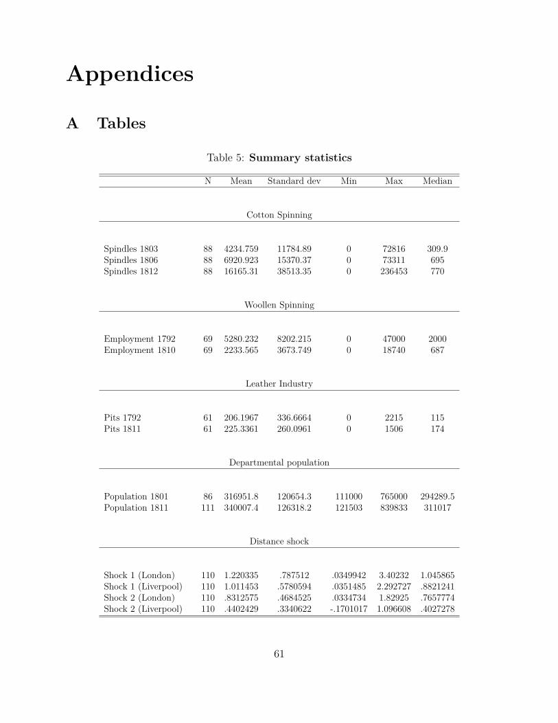
Appendices

A Tables

Table 5: Summary statistics

N Mean Standard dev Min Max Median

Cotton Spinning

Spindles 1803 88 4234.759 11784.89 0 72816 309.9Spindles 1806 88 6920.923 15370.37 0 73311 695Spindles 1812 88 16165.31 38513.35 0 236453 770

Woollen Spinning

Employment 1792 69 5280.232 8202.215 0 47000 2000Employment 1810 69 2233.565 3673.749 0 18740 687

Leather Industry

Pits 1792 61 206.1967 336.6664 0 2215 115Pits 1811 61 225.3361 260.0961 0 1506 174

Departmental population

Population 1801 86 316951.8 120654.3 111000 765000 294289.5Population 1811 111 340007.4 126318.2 121503 839833 311017

Distance shock

Shock 1 (London) 110 1.220335 .787512 .0349942 3.40232 1.045865Shock 1 (Liverpool) 110 1.011453 .5780594 .0351485 2.292727 .8821241Shock 2 (London) 110 .8312575 .4684525 .0334734 1.82925 .7657774Shock 2 (Liverpool) 110 .4402429 .3340622 -.1701017 1.096608 .4027278

61

Table 6: Pre-treatment placebo test

Pre-treatment Baseline effect

(1) (2) (3)Spindles per thous inhabs 1788-93 1794-1803 1803-12

Distance shock (Lo) -0.22 2.78 32.72***(0.78) (1.72) (10.10)

Time FE Yes Yes YesDept FE Yes Yes YesObservations 176 176 176R-squared 0.003 0.034 0.363Number of dept 88 88 88Notes: Col (1) and (2) estimate the effect of the distance shock on spinningcapacity for the periods 1788-93 and 1794-1803 respectively, Col (3) containsthe baseline specification from Table 2, Col (3) for comparison, Standard errorsclustered at the departmental level to account for serial correlation, *** p<0.01,** p<0.05, * p<0.1

Table 7: Fixed effects estimation in levels

Levels Estimation

Spindles (1) (2) (3) (4) (5) (6)

Distance shock (Lo) 14,816*** 22,425*** 20,188*** 23,523*** 24,113**(4,875) (8,120) (7,096) (7,111) (9,190)

Distance shock (Li) 22,802***(8,579)

Time FE No Yes Yes Yes Yes YesDepartmental FE No No Yes Yes Yes YesObservations 176 176 176 176 142 176R-squared 0.189 0.223 0.336 0.330 0.264Number of dept 88 88 88 88 71 88Notes: Depvar is number of spindles, Col (1) - (3) uses cost-distance shock to London with full sample, Col (4)uses weighted distance as an instrument, Col (5) restricts the sample to “ancien regime” France, Col (6) usescost-distance to Liverpool instead of London, Standard errors clustered at the departmental level to accountfor serial correlation, *** p<0.01, ** p<0.05, * p<0.1

62

Table 8: Poisson-fixed effects estimation

Levels Per thousand inhabitants

(1) (2) (3) (4) (5) (6)Spindles (FE) (FE) (FE) (FE) (FE) (FE)

Distance shock (Lo) 0.399* 0.552* 0.429** 0.613**(0.209) (0.295) (0.198) (0.270)

Distance shock (Li) 0.700** 0.736**(0.314) (0.290)

Time FE Yes Yes Yes Yes Yes YesDepartmental FE Yes Yes Yes Yes Yes YesObservations 120 96 120 120 96 120Number of dept 60 48 60 60 48 60Notes: Depvar in Col (1) - (3) is spindles in levels , (3)-(6) is spinldes in per-capita terms,Col (1)and (4) contains the full sample, Col (2) and (5) restricts the sample to “ancien regime”France, Col (3) and (6) use distance to Liverpool instead of London, Standard errors are clus-tered at the departmental level to account for serial correlation, *** p<0.01, ** p<0.05, *p<0.1

63

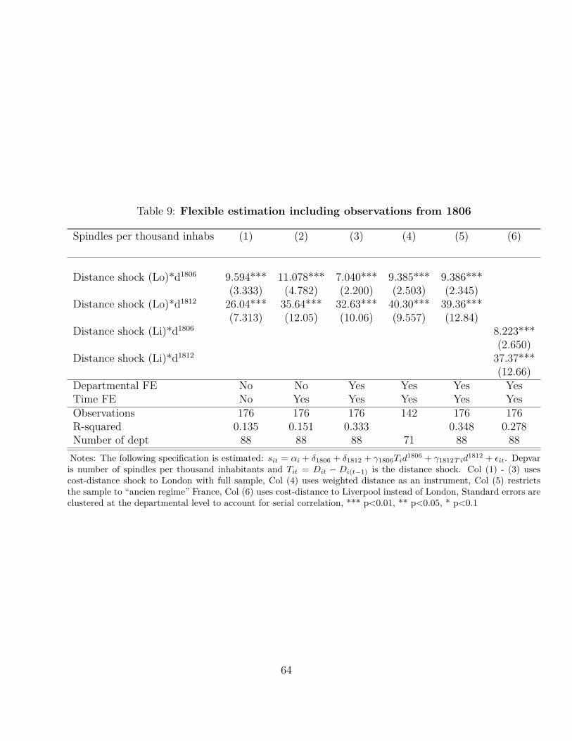
Table 9: Flexible estimation including observations from 1806

Spindles per thousand inhabs (1) (2) (3) (4) (5) (6)

Distance shock (Lo)*d1806 9.594*** 11.078*** 7.040*** 9.385*** 9.386***(3.333) (4.782) (2.200) (2.503) (2.345)

Distance shock (Lo)*d1812 26.04*** 35.64*** 32.63*** 40.30*** 39.36***(7.313) (12.05) (10.06) (9.557) (12.84)

Distance shock (Li)*d1806 8.223***(2.650)

Distance shock (Li)*d1812 37.37***(12.66)

Departmental FE No No Yes Yes Yes YesTime FE No Yes Yes Yes Yes YesObservations 176 176 176 142 176 176R-squared 0.135 0.151 0.333 0.348 0.278Number of dept 88 88 88 71 88 88Notes: The following specification is estimated: sit = αi + δ1806 + δ1812 + γ1806Tid

1806 + γ1812T id1812 + εit. Depvar

is number of spindles per thousand inhabitants and Tit = Dit − Di(t−1) is the distance shock. Col (1) - (3) usescost-distance shock to London with full sample, Col (4) uses weighted distance as an instrument, Col (5) restrictsthe sample to “ancien regime” France, Col (6) uses cost-distance to Liverpool instead of London, Standard errors areclustered at the departmental level to account for serial correlation, *** p<0.01, ** p<0.05, * p<0.1

64

Table 10: Baseline effects with Conley’s standard errors

Per thousand inhabitants Levels

(1) (2) (3) (4) (5) (6)Spindles (FE) (FE) (FE) (FE) (FE) (FE)

Distance shock (Lo) 32.72*** 38.93*** 20,188*** 24,098***(7.778) (12.50) (5,188) (8,493)

Distance shock (Li) 37.54*** 22,802**(14.14) (8,795)

Time FE Yes Yes Yes Yes Yes YesDepartmental FE Yes Yes Yes Yes Yes YesObservations 176 142 176 176 142 176R-squared 0.363 0.372 0.364 0.336 0.354 0.264Number of depts 88 71 88 88 71 88Notes: Depvar is spindles per thousand inhabitants in Columns (1) - (3) and spindles in levels in Columns(4) - (6). Columns (1) and (3) estimate the baseline specification, Columns (2) and (4) restrict the sample todepartments belonging to “ancien regime” France, Columns (3) and (6) calculate the distance shock usingLiverpool as the source port instead of London. Spatial HAC standard errors (Conley, 2008) calculatedusing Hsiang’s (2010) code. Correlation across space is assumed to be zero for departments more than 250km apart (using the prefecture as the location of the department). Serial correlation in the departmentaldimension is also accounted for, *** p<0.01, ** p<0.05, * p<0.1

65

Table11:Pr

iceof

cotton

wool

atdiffe

rent

locatio

ns(fr

ancs

perkilogram

me)

Levantinecotton

Georgia

cotton

Brazilian

cotton

Leipzig

Beau

caire

Paris

Strasbou

rgDuty

Lond

onLe

ipzig

Beau

caire

Paris

Duty

Lond

onLe

ipzig

Beau

caire

Paris

Duty

1806

4.4-4.48

4.11

0.6

2.78-30.2

4.04

0.6

4.64-4.87

6.8-7.04

6.8-7.3

0.6

1807

4.32

4.5

4.7

0.6

2.78-3.25

55

4.5-6.6

0.6

4.87-5.1

7.6

70.6

1808

7.68

11.6-12.07

11-13.25

0.6

5.57-6.96

12.8

8.8-14.6

0.6

4.87-5.33

19.2

14.9-15

0.6

1809

6.08-6.16

70.6

2.32-2.78

10.4

0.6

4.64-5.51

2012-13.5

15-17.5

0.6

1810

6.56-6.8

6.93

8-10

8-8.5

2-4

3.94-4.41

7.6

85.8-6.26

16.8

12-14

81811

4.48

9-9.2

8-9

2-4

1.52-2.09

5.6-6.04

11-18

83.25-3.48

8-8.48

10.2

16-1

6.4

81812

4.16

58.5-10

2-4

2.55-3.02

4.16

83.94-4.64

11.2

13-13.5

81813

4.48

2-4

3.71-4.41

6.08

85.33-5.57

10.4

8Notes:Dutyis

theim

port

tariff

(francspe

rkilogram

me)

paid

upon

entryinto

theFrench

Empire.W

here

possible,d

atais

consist

entacross

time.

ForLe

ipzig,

data

isfrom

thean

nual

Easter

Fair,

forBeaucaire

itis

from

thean

nual

fair

inJu

ly.To

ensure

compa

rabilityof

prices

across

Fran

ce,w

here

possible,P

aris

prices

arechosen

tocoincide

with

thefair

inBeaucaire

andthesame

istrue

forStrasbou

rg.Datasources:

Lond

on:To

oke(1928),S

trasbo

urg:

Ellis

(1991,

p.169),B

eaucaire:AN/F

12/1254B

,Leipzig:Heckscher

(1991,

p.274),P

aris:

AN/F

12/533

1807-1809,

AN/f12/633

Janu

ary(1811)

andHeckscher

(1991,

p.274)

otherw

iseC

forsources

66

B Figures

Figure 14: Smuggling routes using shortest distance approach for Rouen

1 Notes: Possible routes for smuggling between London and Rouen during the Blockade. Smuggling centresare Heligoland, Gibraltar, Gothenburg and Malta. Goods can be smuggled from here to ports shown ingrey. The algorithm picks the shortest smuggling route to get from London to Rouen.

67

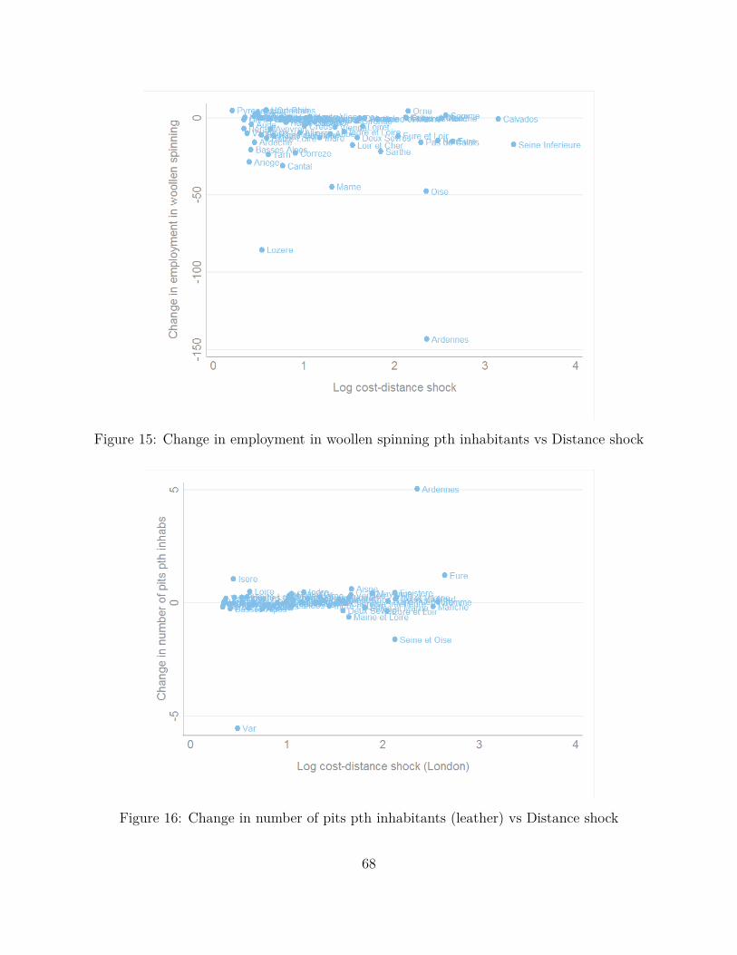
Figure 15: Change in employment in woollen spinning pth inhabitants vs Distance shock

Figure 16: Change in number of pits pth inhabitants (leather) vs Distance shock

68

Figure 17: Capital labour ratio in mechanised spinning vs distance shock

1 Notes: Capital labour ratio is calculated as the number of spindles divided by labour employed inmechanised spinning in 1812. The cost-distance shock is calculated based on the shortest route algorithm(measure 1). The point estimate is -11.5575 ( se 11.41808).

69

(a) Mean flow rate (b) Proximity to coal

Figure 18: Geographic fundamentals

Notes: The mean flow rates across the French Empire are calculated using the average monthly flow-rate(m3/s) for each station across the historical boundaries of the French Empire. The mean for eachdepartment is then calculated, and the natural log of this mean gives the mean-flow rate for eachdepartment. Access to coal uses the Fernihough-O’Rourke (2014) dataset. To calculate the departmentaldatapoint I use the minimum distance to any of Europe’s major coalfields from the capital of eachdepartment. Where data for the capital is not available, I use the closest city from the dataset. Thisdistance is transformed into a proximity measure using the author’s measure. See Appendix C for details.

70

C Data Sources

1. French Textile Data (cotton, wool, leather): Archives Nationales, Paris F/12

2. French and British cotton yarn prices: Archives Nationales, Paris F/12

3. French raw cotton prices: Archives Nationales, Paris F/12

4. French Trade Data: collected by Guillaume Daudin from Archives Nationales, ParisF/12

5. Shipping data: Lloyds List, 1787-1814, digitised by Google, made available by theHathi Trust

6. French departmental population: Chabert, A., Lefebvre, G. (1949). Essai sur lesmouvements des revenus et de l’activité économique en France de 1798 à 1820. Librairiede Médicis

7. Consumption of Raw Cotton: Mitchell, B. R. (2007). International historical statistics.Europe, 1750-2005 Palgrave Macmillan

8. British Trade Data: Mitchell, B. R. (1988). Abstract of British historical statistics.CUP Archive.

9. French Industrial Census, 1839-47: Chanut, Jean-Marie, Jean Heffer, Jacques Mairesse,Gilles Postel-Vinay, Frédéric Boccara, Pierre Sicsic, André Straus, and Patrick Verley(2000). L’industrie française au milieu du 19 e siècle(les enquêtes de la statistiquegénérale en France). Recherches d’histoire et de sciences sociales.

10. US Trade Data: Pitkin, Timothy (1817). A statistical view of the commerce of theUnited States of America: its connection with agriculture and manufactures: and anaccount of the public debt, revenues, and expenditures of the United States. With abrief review of the trade, agriculture, and manufactures of the colonies, previous totheir independence. Accompanied with tables, illustrative of the principles and objectsof the work. James Eastburn Company.

11. Coal: Fernihough, A., O’Rourke, K. H. (2014). Coal and the European IndustrialRevolution (No. w19802). National Bureau of Economic Research.

12. Mean-flow rates: European Water Archive, EURO-FRIEND River Discharge Data

71

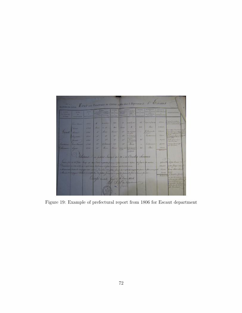
Figure 19: Example of prefectural report from 1806 for Escaut department

72

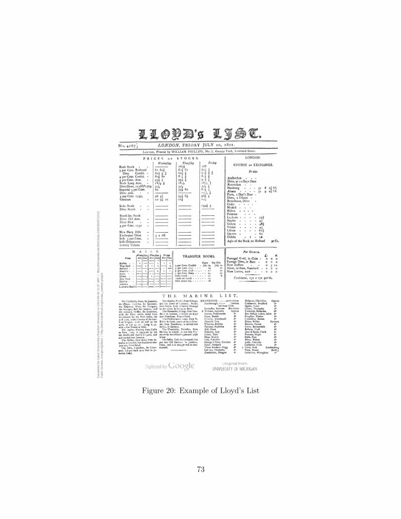
Figure 20: Example of Lloyd’s List

73