Embed Size (px)
Citation preview
OECD Science, Technology and Industry Working Papers2003/15
Carbon Dioxide EmissionsEmbodied in International
Trade of Goods
Nadim Ahmad,Andrew Wyckoff
https://dx.doi.org/10.1787/421482436815
Unclassified DSTI/DOC(2003)15 Organisation de Coopération et de Développement Economiques Organisation for Economic Co-operation and Development 03-Nov-2003 ___________________________________________________________________________________________
English text only DIRECTORATE FOR SCIENCE, TECHNOLOGY AND INDUSTRY
CARBON DIOXIDE EMISSIONS EMBODIED IN INTERNATIONAL TRADE OF GOODS STI WORKING PAPER 2003/15
Nadim Ahmad and Andrew Wyckoff
JT00152835
Document complet disponible sur OLIS dans son format d'origine Complete document available on OLIS in its original format
DST
I/DO
C(2003)15
Unclassified
English text only
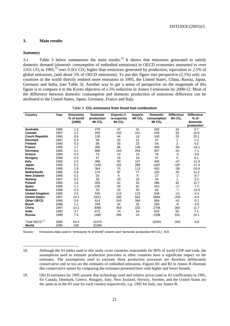
DSTI/DOC(2003)15
2
STI Working Paper Series
The Working Paper series of the OECD Directorate for Science, Technology and Industry is designed to make available to a wider readership selected studies prepared by staff in the Directorate or by outside consultants working on OECD projects. The papers included in the series cover a broad range of issues, of both a technical and policy-analytical nature, in the areas of work of the DSTI. The Working Papers are generally available only in their original language – English or French – with a summary in the other.
Comments on the papers are invited, and should be sent to the Directorate for Science, Technology and Industry, OECD, 2 rue André-Pascal, 75775 Paris Cedex 16, France.
The opinions expressed in these papers are the sole responsibility of the author(s) and do not necessarily reflect those of the OECD or of the governments of its member countries.
http://www.oecd.org/sti/working-papers
Copyright OECD, 2003 Applications for permission to reproduce or translate all or part of this material should be made to: OECD Publications, 2 rue André-Pascal, 75775 Paris, Cedex 16, France.
DSTI/DOC(2003)15
3
CARBON DIOXIDE EMISSIONS EMBODIED IN INTERNATIONAL TRADE OF GOODS
Nadim Ahmad and Andrew Wyckoff
Abstract
Efforts such as the Kyoto Protocol to reduce emissions that may be linked to climate change focus on six greenhouse gases (GHG). Carbon dioxide is by far the largest of these by volume, representing about 80% of the total emissions of these six gases. Almost all carbon dioxide is emitted during the combustion of fossil fuels and OECD countries account for over half of the total carbon dioxide emission in the world while an additional four countries (Brazil, China, India and Russia) together account for a further quarter of the global total. Many policies designed to reduce these emissions set emission reduction goals based on some previous level (e.g. 1990 in the case of Kyoto for many countries) which is used as a benchmark for success and compliance to the protocol. But changes in emissions at the national level can occur for many reasons: including the relocation of production abroad, and/or by import substitution. This may have a negligible impact on global emissions but, if the imports use more GHG intensive production processes than the domestically produced goods that they displace, global emissions could well be higher. The objective of this paper is to explore the role of trade in goods in this context by creating an indicator that estimates CO2 emissions related to domestic demand, for 24 countries (responsible for 80% of global CO2 emissions), as a complement to the more common indicator of emissions associated with domestic production of emissions, such as that used in the Kyoto Protocol. Using conservative assumptions the paper shows that estimates of CO2 emissions generated to satisfy domestic demand in the OECD in 1995 were 5% higher than emissions related to production. To put this figure into perspective only six countries in the world directly emitted more CO2 in 1995.
DSTI/DOC(2003)15
4
LES EMISSIONS DE DIOXYDE DE CARBONE INCORPOREES DANS LES ECHANGES INTERNATIONAUX DE MARCHANDISES
Nadim Ahmad et Andrew Wyckoff
Résumé
Des initiatives telles que le Protocole de Kyoto qui visent à réduire les émissions susceptibles de contribuer au changement climatique portent essentiellement sur six gaz à effet de serre (GES). Le dioxyde de carbone est de loin le plus important d'entre eux en volume, puisqu'il représente environ 80 % des émissions totales de ces six gaz. La quasi-totalité des émissions de ce gaz sont imputables à l'utilisation de combustibles fossiles et les pays de l'OCDE sont responsables de plus de la moitié des émissions totales de dioxyde de carbone dans le monde, tandis que quatre autres pays (Brésil, Chine, Inde et Russie) représentent ensemble un quart du total. Nombre de politiques visant à réduire ces émissions fixent des objectifs de réduction fondées sur un niveau antérieur (dans le cas de Kyoto, par exemple, celui de 1990 pour de nombreux pays) qui sert de repère pour juger du respect du protocole et de sa réussite. Or l'évolution des émissions au niveau national peut s'expliquer par de nombreuses causes, notamment la relocalisation d'activités de production à l'étranger et/ou la substitution de produits importés aux productions nationales. Il se peut que l'impact sur les émissions globales soit négligeable mais, si les produits importés ont été obtenus à l'aide de procédés à plus forte intensité d'émissions de GES que celle des productions nationales qu'ils remplacent, les émissions globales pourraient bien être supérieures. L'objet de ce document est d'étudier le rôle des échanges de marchandises dans ce contexte en créant un indicateur qui estime les émissions de CO2 par rapport à la demande intérieure, pour 24 pays (responsables de 80 % des émissions globales de CO2), afin de compléter l'indicateur plus courant associé à la production nationale d'émissions, comme celui utilisé dans le Protocole de Kyoto. Sur la base d'hypothèses modérées, ce document montre que les estimations des émissions de CO2 engendrées pour répondre à la demande intérieure des pays de l'OCDE en 1995 ont été supérieures de 5 % aux émissions engendrées par la production. Pour situer ce chiffre dans son contexte, seuls six pays dans le monde ont directement émis plus de CO2 en 1995.
DSTI/DOC(2003)15
5
TABLE OF CONTENTS
EXECUTIVE SUMMARY ............................................................................................................................ 6
Key findings ................................................................................................................................................ 7
CARBON DIOXIDE EMISSIONS EMBODIED IN INTERNATIONAL TRADE OF GOODS ................ 9
1. Introduction ...................................................................................................................................... 9 CO2 emissions – background................................................................................................................... 9 The Kyoto Protocol and international trade........................................................................................... 14
2. Methodology .................................................................................................................................. 16 Data sources........................................................................................................................................... 18 CO2 emissions from industrial production............................................................................................. 18 Assumptions .......................................................................................................................................... 19 Time-series of embodied emissions....................................................................................................... 19
3. Main results .................................................................................................................................... 21 Summary................................................................................................................................................ 21 Main features ......................................................................................................................................... 23 Emission factors by sector ..................................................................................................................... 24
4. Summary of main results ............................................................................................................ 31
ANNEX A – EMBODIED EMISSIONS FIVE YEAR GROWTH (TENTATIVE ESTIMATES)............. 32
Growth in international trade, 1990-2000 ............................................................................................. 34 Embodied emissions .............................................................................................................................. 35 CO2 emissions – domestic consumption versus domestic production by country................................. 38
ANNEX B – DETAILED METHODOLOGY............................................................................................. 46
The input-output framework.................................................................................................................. 46 Data........................................................................................................................................................ 47 Assumptions .......................................................................................................................................... 51 Estimating emission factors in countries where IO data are not available ............................................ 51 Adjusting for differences in electricity generation ................................................................................ 51 Gas and oil – extraction & refining ....................................................................................................... 51 Sensitivity to assumptions for non-IO countries.................................................................................... 52 Coherence between IEA emissions data and input-output tables .......................................................... 53 Bilateral trade data – allocation of imports to industries ....................................................................... 53 Differences in IO years.......................................................................................................................... 54 Interpreting emission factors – Table 4 ................................................................................................. 54 Electricity............................................................................................................................................... 57 Embodied emissions including transportation, services and electricity auto-producer emissions ........ 60
DSTI/DOC(2003)15
6
EXECUTIVE SUMMARY1
1. Efforts such as the Kyoto Protocol to reduce emissions that may be linked to climate change focus on six greenhouse gases (GHG). Carbon dioxide is by far the largest of these by volume, representing about 80% of the total emissions of these six gases. Almost all carbon dioxide is emitted during the combustion of fossil fuels and OECD countries account for over half of the total carbon dioxide emission in the world while an additional four countries (Brazil, China, India and Russia) together account for a further quarter of the global total. Many policies designed to reduce these emissions set emission reduction goals based on some previous level (e.g. 1990 in the case of Kyoto for many countries) which is used as a benchmark for success and compliance to the protocol. But changes in emissions at the national level can occur for many reasons: including the relocation of production abroad, and/or by import substitution. This may have a negligible impact on global emissions but, if the imports use more GHG intensive production processes than the domestically produced goods that they displace, global emissions could well be higher.
2. The objective of the analysis presented here is to explore the role of trade in goods, (including mining, refining, agriculture, electricity as well as manufacturing), by OECD economies in their CO2
emissions by creating an indicator that estimates the emissions associated with the domestic consumption2 of these economies as a complement to the more common indicator of emissions associated with domestic production3 of emissions, such as that used in the Kyoto Protocol. In this sense the purpose of this paper is to derive an experimental indicator that illustrates the potential importance of emissions related to the import and export of goods. No attempt is made to evaluate existing policies using this experimental indicator. In brief the concept of consumption excludes emissions associated with exports and includes emissions generated in the production of imports by tracing these imports back to their place of origin and estimating their emissions based on the production processes used to create them. It does this by developing an analytical framework, based on input-output tables, that attempts to measure the indirect carbon dioxide requirements of economies by measuring carbon dioxide emissions from fossil fuel-use embodied in imports and exports both directly and indirectly. Twenty-four countries, responsible in 1995 for 80% of global emissions and global GDP in nominal prices (World Bank), are covered in this study. By
1 . This report was prepared by Nadim Ahmad and Andrew Wyckoff of the Economic Analysis and Statistics
Division of the Directorate for Science Technology and Industry (DSTI) as a methodological contribution to the OECD’s work on sustainable development indicators. The authors would like to pay special thanks for the invaluable contributions of Paul Atkinson, and Colin Webb also of DSTI, and the members of the OECD’s Roundtable on Sustainable Development (Anne Harrison, Simon Upton and Vitalis Vangelis). A preliminary version of this paper was presented to the Working Group on Environmental Information and Outlooks (WGEIO) and at the OECD Statistics Directorate’s Workshop on Sustainable Development, and this final version reflects the comments received by these groups.
2. Analogous to total domestic final demand where emissions from household and government final consumption and investment, including changes in business inventories are calculated regardless of the fact that the goods being consumed were imported or produced domestically.
3. Where the emissions from only domestically produced products for household and government final consumption and investment, including changes in business inventories are included as well as emissions associated with the production of products destined for export.
DSTI/DOC(2003)15
7
presenting emissions on the basis of domestic consumption it is possible to gain additional insight into the possible causes of changes in emissions in any particular country and better assess the impact of industrial change on global emissions.
3. A wide range of formal (e.g. United Nations Framework Convention on Climate Change, OECD Annex I Experts Group) and 'informal' (e.g. Centre for Clear Air Policy Future Actions Dialogue, Pew Centre, various NGOs) groups have already begun to consider how the international climate change policy regime might change for the post-2012 period. One key criteria (among others) being explored is that of "responsibility"; in particular, whether the responsibility for emissions lies with consumers or producers. Selecting one or the other requires a consideration of the issue of equity and the availability of statistics that can be used to measure either indicator. The former (equity issue) is beyond the scope of this paper but the latter (statistics) is not.
4. In this context it is clear that consumption-based measures are more data-intensive than production-based measures and, moreover, require more assumptions, (e.g. those relating to input-output tables, market exchange rate conversions) and these factors limit the reliability that can currently be placed on consumption-based measures. However, the paper demonstrates that it is possible to estimate lower-bound consumption-based indicators for emissions from fossil fuel combustion at least. This suggests that consumption-based indicators would be useful complements to the more traditional production-based indicators. In addition, increasing numbers of national statistical offices are developing input-output tables (and more regularly) and, so, the reliability of consumption-based estimates can be expected to improve over time.
Key findings
• The estimates developed here suggest that emissions associated with the domestic consumption of products are higher than the domestic production of emissions for the OECD as whole and significantly so for some countries.
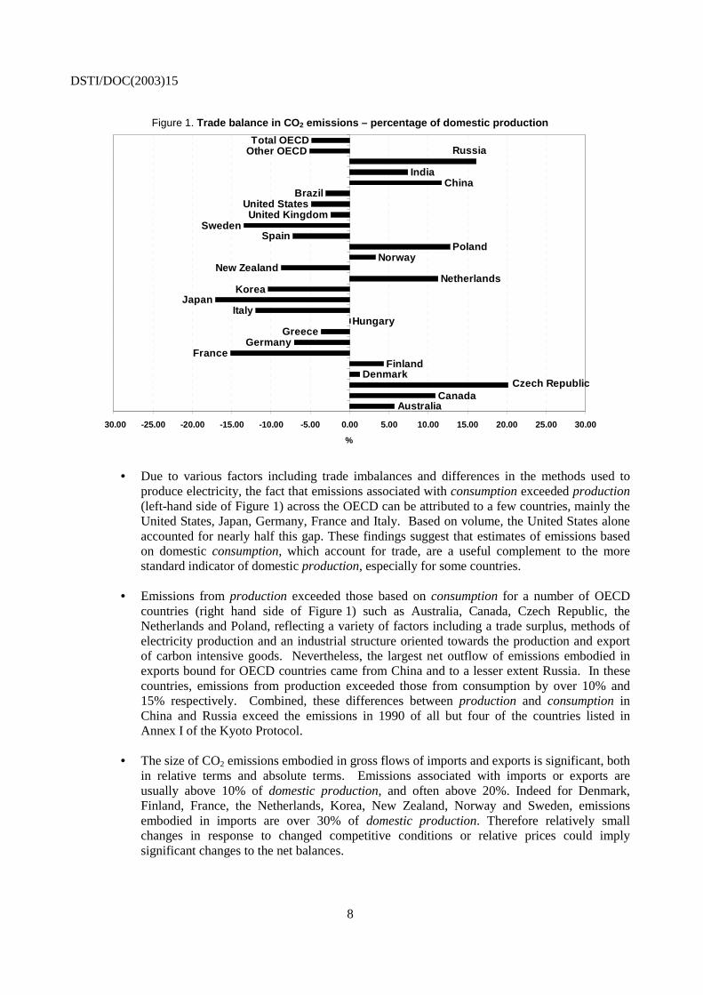
• Emissions generated to satisfy domestic demand (domestic consumption of embodied emissions) in OECD economies are estimated at over 12Gt CO2 in 1995,4 over 0.5Gt CO2 higher than emissions generated by production. This difference, which is reflected in the balance of emissions embodied in imports and those embodied in exports, is equivalent to 2.5% of global emissions, (and about 5% of OECD emissions) (Figure 1). To put this figure (2.5%) into perspective only six countries in the world directly emitted more emissions in 1995. To give another sense of the magnitude of the 5% difference between domestic consumption and production, it is roughly comparable to the 5% reduction target set by the Kyoto Protocol for 2008-2012 for Annex I countries. For many individual countries, the emissions associated with consumption are often +/-10% greater or less than domestic production.
4. OECD estimates for 1995 assume that technology used and relative prices (and so IO coefficients) in 1995,
for Canada, Denmark, Greece, Hungary, Italy. New Zealand, Norway, Sweden, and the United States are the same as in the IO year for each country respectively, e.g. 1992 for Italy.
DSTI/DOC(2003)15
8
Figure 1. Trade balance in CO2 emissions – percentage of domestic production
Canada
DenmarkFinland
FranceGermany
GreeceHungary
ItalyJapan
KoreaNetherlands
New ZealandNorway
PolandSpain
SwedenUnited Kingdom
United StatesBrazil
ChinaIndia
Other OECDTotal OECD
Australia
Russia
Czech Republic
30.00 -25.00 -20.00 -15.00 -10.00 -5.00 0.00 5.00 10.00 15.00 20.00 25.00 30.00
%
• Due to various factors including trade imbalances and differences in the methods used to produce electricity, the fact that emissions associated with consumption exceeded production (left-hand side of Figure 1) across the OECD can be attributed to a few countries, mainly the United States, Japan, Germany, France and Italy. Based on volume, the United States alone accounted for nearly half this gap. These findings suggest that estimates of emissions based on domestic consumption, which account for trade, are a useful complement to the more standard indicator of domestic production, especially for some countries.
• Emissions from production exceeded those based on consumption for a number of OECD countries (right hand side of Figure 1) such as Australia, Canada, Czech Republic, the Netherlands and Poland, reflecting a variety of factors including a trade surplus, methods of electricity production and an industrial structure oriented towards the production and export of carbon intensive goods. Nevertheless, the largest net outflow of emissions embodied in exports bound for OECD countries came from China and to a lesser extent Russia. In these countries, emissions from production exceeded those from consumption by over 10% and 15% respectively. Combined, these differences between production and consumption in China and Russia exceed the emissions in 1990 of all but four of the countries listed in Annex I of the Kyoto Protocol.
• The size of CO2 emissions embodied in gross flows of imports and exports is significant, both in relative terms and absolute terms. Emissions associated with imports or exports are usually above 10% of domestic production, and often above 20%. Indeed for Denmark, Finland, France, the Netherlands, Korea, New Zealand, Norway and Sweden, emissions embodied in imports are over 30% of domestic production. Therefore relatively small changes in response to changed competitive conditions or relative prices could imply significant changes to the net balances.
DSTI/DOC(2003)15
9
CARBON DIOXIDE EMISSIONS EMBODIED IN INTERNATIONAL TRADE OF GOODS
1. Introduction
CO2 emissions – background
1.1 The Intergovernmental Panel on Climate Change (IPCC), created in 1988 to assess the scientific, technical and socio-economic information relevant to anthropogenic emissions, established in its second report in 1995 a link between these emissions and climate change, stating that “the balance of evidence suggests a discernible human influence on global climate”. The release of this report culminated in the adoption of the Kyoto Protocol to the United Nations Framework Convention on Climate Change (UNFCCC) in December 1997.
1.2 The Kyoto Protocol (Box 1) set out a framework for measuring and reducing these emissions, and, acknowledging that economies are at different stages of development and that developed economies produce the majority of GHG emissions. The protocol encourages developed and transition economies, (known as Annex I countries5), to take the lead in limiting their emissions. Non-Annex I countries, made up largely of developing economies, are also encouraged to reduce emissions but, given their different stages of economic development, have no emissions targets identified in the protocol.
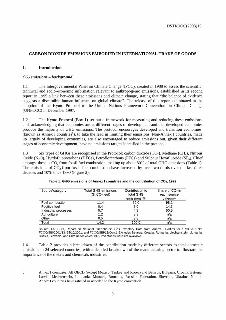
1.3 Six types of GHGs are recognised in the Protocol: carbon dioxide (CO2), Methane (CH4), Nitrous Oxide (N2O), Hyrdofluorocarbons (HFCs), Petroflorcarbons (PFCs) and Sulphur Hexafluoride (SF6). Chief amongst these is CO2 from fossil fuel combustion, making up about 80% of total GHG emissions (Table 1). The emissions of CO2 from fossil fuel combustion have increased by over two-thirds over the last three decades and 10% since 1990 (Figure 2).
Table 1. GHG emissions of Annex I countries and the contribution of CO2, 1999
Source\category Total GHG emissions (Gt CO2, eqt)
Contribution to total GHG
emissions %
Share of CO2 in each source
category Fuel combustion 11.4 80.0 98.2 Fugitive fuel 0.4 3.0 14.3 Industrial processes 0.7 4.9 50.5 Agriculture 1.2 8.3 n/a Other 0.5 3.8 n/a Total 14.2 100.0 n/a
Source: UNFCCC, Report on National Greenhouse Gas Inventory Data from Annex I Parties for 1990 to 1999, FCCC/SBI/2001/13, 25/10/2001, and FCCC/SBI/13/Corr.1 Excludes Belarus, Croatia, Romania, Liechtenstein, Lithuania, Russia, Slovenia, and Ukraine for which 1999 inventories were not available.
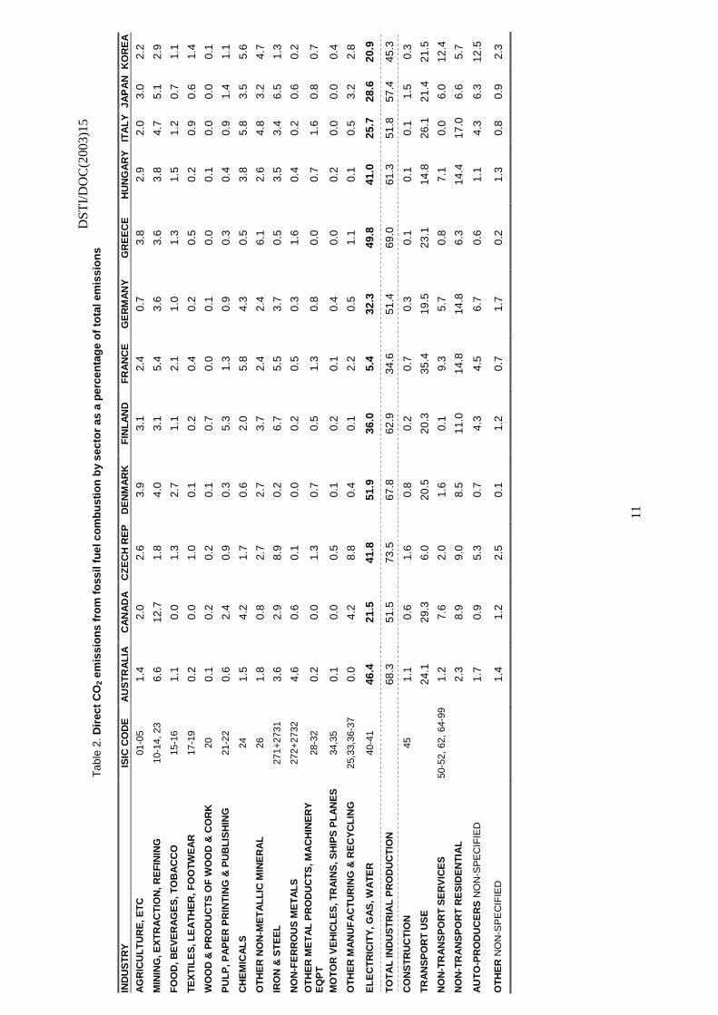
1.4 Table 2 provides a breakdown of the contribution made by different sectors to total domestic emissions in 24 selected countries, with a detailed breakdown of the manufacturing sector to illustrate the importance of the metals and chemicals industries.
5. Annex I countries: All OECD (except Mexico, Turkey and Korea) and Belarus, Bulgaria, Croatia, Estonia,
Latvia, Liechtenstein, Lithuania, Monaco, Romania, Russian Federation, Slovenia, Ukraine. Not all Annex I countries have ratified or acceded to the Kyoto convention.
DSTI/DOC(2003)15
10
Box 1. The Kyoto Protocol
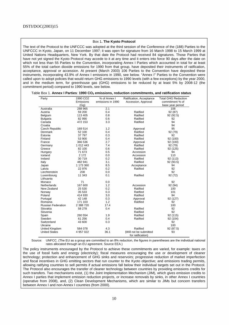
The text of the Protocol to the UNFCCC was adopted at the third session of the Conference of the (188) Parties to the UNFCCC in Kyoto, Japan, on 11 December 1997; it was open for signature from 16 March 1998 to 15 March 1999 at United Nations Headquarters, New York. By that date the Protocol had received 84 signatures. Those Parties that have not yet signed the Kyoto Protocol may accede to it at any time and it enters into force 90 days after the date on which not less than 55 Parties to the Convention, incorporating Annex I Parties which accounted in total for at least 55% of the total carbon dioxide emissions for 1990 from that group, have deposited their instruments of ratification, acceptance, approval or accession. At present (March 2003) 106 Parties to the Convention have deposited these instruments, incorporating 43.9% of Annex I emissions in 1990, see below. “Annex I” Parties to the Convention were called upon to adopt policies that would return GHG emissions to 1990 levels (with a few exceptions) by the year 2000, and in the medium term, for greenhouse gas (GHG) emissions to be reduced by at least 5% by 2008-12 (the commitment period) compared to 1990 levels, see below.
Table Box 1. Annex I Parties: 1990 CO2 emissions, reduction commitments, and ratification status
Party 1990 CO2 Emissions
(Gg)
% of Annex I emissions in 1990
Ratification, Acceptance Accession, Approval
Total GHG Reduction commitment % of base year period
Australia 288 965 2.1 108 Austria 59 200 0.4 Ratified 92 (87) Belgium 113 405 0.8 Ratified 92 (92.5) Bulgaria 82 990 0.6 Ratified 92 Canada 472 153 3.3 Ratified 94 Croatia 94 Czech Republic 169 514 1.2 Approval 95 Denmark 52 100 0.4 Ratified 92 (79) Estonia 37 797 0.3 Ratified 92 Finland 53 900 0.4 Ratified 92 (100) France 366 536 2.7 Approval 92 (100) Germany 1 012 443 7.4 Ratified 92 (79) Greece 82 100 0.6 Ratified 92 (125) Hungary 71 673 0.5 Accession 94 Iceland 2 172 0.0 Accession 110 Ireland 30 719 0.2 Ratified 92 (113) Italy 482 941 3.1 Ratified 92 (93.5) Japan 1 173 360 8.5 Acceptance 94 Latvia 22 976 0.2 Ratified 92 Liechtenstein 208 0.0 92 Luxembourg 11 343 0.1 Ratified 92 (72) Lithuania Monaco 71 0.0 92 Netherlands 167 600 1.2 Accession 92 (94) New Zealand 25 530 0.2 Ratified 100 Norway 35 533 0.3 Ratified 101 Poland 414 930 3.0 Ratified 94 Portugal 42 148 0.3 Approval 92 (127) Romania 171 103 1.2 Ratified 92 Russian Federation 2 388 720 17.4 100 Slovakia 58 278 0.4 Ratified 92 Slovenia Ratified 92 Spain 260 554 1.9 Ratified 92 (115) Sweden 61 256 0.4 Ratified 92 (104) Switzerland 43 600 0.3 92 Ukraine 100 United Kingdom 584 078 4.3 Ratified 92 (87.5) United States 4 957 022 36.1 (Will not be submitted
for ratification) 93
Source: UNFCC. (The EU as a group are committed to an 8% reduction, the figures in parentheses are the individual national rates allocated through an EU agreement. Source EEA.)
The policy instruments encouraged by the Protocol to achieve these commitments are varied, for example: taxes on the use of fossil fuels and energy (electricity); fiscal measures encouraging the use or development of cleaner technology; protection and enhancement of GHG sinks and reservoirs; progressive reduction of market imperfection and fiscal incentives in GHG emitting sectors that run counter to the Kyoto objective; and emissions trading permits, allowing ratifying countries to sell permits if actual emissions fall below their individual targets set out in the Protocol. The Protocol also encourages the transfer of cleaner technology between countries by providing emissions credits for such transfers. Two mechanisms exist, (1) the Joint Implementation Mechanism (JIM), which gives emission credits to Annex I parties that implement emission reduction projects, or increase removals by sinks, in other Annex I countries (operative from 2008), and, (2) Clean Development Mechanisms, which are similar to JIMs but concern transfers between Annex I and non-Annex I countries (from 2000).
D
STI/
DO
C(2
003)
15
11
Tab
le 2
. Dir
ect
CO
2 em
issi
on
s fr
om
fo
ssil
fuel
co
mb
ust
ion
by
sect
or
as a
per
cen
tag
e o
f to
tal e
mis
sio
ns
IND
US
TR
Y
ISIC
CO
DE
A
US
TR
AL
IA
CA
NA
DA
C
ZE
CH
RE
P
DE
NM
AR
K
FIN
LA
ND
F
RA
NC
E
GE
RM
AN
Y
GR
EE
CE
H
UN
GA
RY
IT
AL
Y
JAP
AN
K
OR
EA
AG
RIC
UL
TU
RE
, ET
C
01-0
5 1.
4 2.
0 2.
6 3.
9 3.
1 2.
4 0.
7 3.
8 2.
9 2.
0 3.
0 2.
2
MIN
ING
, EX
TR
AC
TIO
N, R
EF
ININ
G
10-1
4, 2
3 6.
6 12
.7
1.8
4.0
3.1
5.4
3.6
3.6
3.8
4.7
5.1
2.9
FO
OD
, BE
VE
RA
GE
S, T
OB
AC
CO
15
-16
1.1
0.0
1.3
2.7
1.1
2.1
1.0
1.3
1.5
1.2
0.7
1.1
TE
XT
ILE
S, L
EA
TH
ER
, FO
OTW
EA
R
17-1
9 0.
2 0.
0 1.
0 0.
1 0.
2 0.
4 0.
2 0.
5 0.
2 0.
9 0.
6 1.
4
WO
OD
& P
RO
DU
CT
S O
F W
OO
D &
CO
RK
20
0.
1 0.
2 0.
2 0.
1 0.
7 0.
0 0.
1 0.
0 0.
1 0.
0 0.
0 0.
1
PU
LP
, PA
PE
R P
RIN
TIN
G &
PU
BL
ISH
ING
21
-22
0.6
2.4
0.9
0.3
5.3
1.3
0.9
0.3
0.4
0.9
1.4
1.1
CH
EM
ICA
LS
24
1.
5 4.
2 1.
7 0.
6 2.
0 5.
8 4.
3 0.
5 3.
8 5.
8 3.
5 5.
6
OT
HE
R N
ON
-ME
TA
LL
IC M
INE
RA
L
26
1.8
0.8
2.7
2.7
3.7
2.4
2.4
6.1
2.6
4.8
3.2
4.7
IRO
N &
ST
EE
L
271+
2731
3.
6 2.
9 8.
9 0.
2 6.
7 5.
5 3.
7 0.
5 3.
5 3.
4 6.
5 1.
3
NO
N-F
ER
RO
US
ME
TA
LS
27
2+27
32
4.6
0.6
0.1
0.0
0.2
0.5
0.3
1.6
0.4
0.2
0.6
0.2
OT
HE
R M
ET
AL
PR
OD
UC
TS
, MA
CH
INE
RY
E
QP
T
28-3
2 0.
2 0.
0 1.
3 0.
7 0.
5 1.
3 0.
8 0.
0 0.
7 1.
6 0.
8 0.
7
MO
TO
R V
EH
ICL
ES
, TR
AIN
S, S
HIP
S P
LA
NE
S
34,3
5 0.
1 0.
0 0.
5 0.
1 0.
2 0.
1 0.
4 0.
0 0.
2 0.
0 0.
0 0.
4
OT
HE
R M
AN
UF
AC
TU
RIN
G &
RE
CY
CL
ING
25
,33,
36-3
7 0.
0 4.
2 8.
8 0.
4 0.
1 2.
2 0.
5 1.
1 0.
1 0.
5 3.
2 2.
8
EL
EC
TR
ICIT
Y, G
AS
, WA
TE
R
40-4
1 46
.4
21.5
41
.8
51.9
36
.0
5.4
32.3
49
.8
41.0
25
.7
28.6
20
.9
TO
TA
L IN
DU
ST
RIA
L P
RO
DU
CT
ION
68.3
51
.5
73.5
67
.8
62.9
34
.6
51.4
69
.0
61.3
51
.8
57.4
45
.3
CO
NS
TR
UC
TIO
N
45
1.1
0.6
1.6
0.8
0.2
0.7
0.3
0.1
0.1
0.1
1.5
0.3
TR
AN
SP
OR
T U
SE
24.1
29
.3
6.0
20.5
20
.3
35.4
19
.5
23.1
14
.8
26.1
21
.4
21.5
NO
N-T
RA
NS
PO
RT
SE
RV
ICE
S
50-5
2, 6
2, 6
4-99
1.
2 7.
6 2.
0 1.
6 0.
1 9.
3 5.
7 0.
8 7.
1 0.
0 6.
0 12
.4
NO
N-T
RA
NS
PO
RT
RE
SID
EN
TIA
L
2.
3 8.
9 9.
0 8.
5 11
.0
14.8
14
.8
6.3
14.4
17
.0
6.6
5.7
AU
TO
-PR
OD
UC
ER
S N
ON
-SP
EC
IFIE
D
1.
7 0.
9 5.
3 0.
7 4.
3 4.
5 6.
7 0.
6 1.
1 4.
3 6.
3 12
.5
OT
HE
R N
ON
-SP
EC
IFIE
D
1.
4 1.
2 2.
5 0.
1 1.
2 0.
7 1.
7 0.
2 1.
3 0.
8 0.
9 2.
3
DST
I/D
OC
(200
3)15
12
IN
DU
ST
RY
N
ET
HE
RL
AN
DS
NE
W Z
’LA
ND
N
OR
WA
Y
PO
LA
ND
S
PA
IN
SW
ED
EN
U
K
US
B
RA
ZIL
IN
DIA
C
HIN
A R
US
SIA
WO
RL
D
AG
RIC
UL
TU
RE
, ET
C
5.4
2.6
6.0
4.0
2.3
2.8
0.5
0.9
5.3
0.2
2.7
1.4
1.9
MIN
ING
, EX
TR
AC
TIO
N, R
EF
ININ
G
9.2
5.1
36.4
4.
2 5.
9 4.
3 7.
3 5.
0 8.
5 3.
0 5.
1 3.
3 5.
6
FO
OD
, BE
VE
RA
GE
S, T
OB
AC
CO
1.
8 0.
3 1.
4 2.
4 1.
9 1.
5 1.
4 1.
0 1.
7 0.
4 2.
0 0.
5 1.
1
TE
XT
ILE
S, L
EA
TH
ER
, FO
OTW
EA
R
0.2
0.0
0.1
0.7
0.8
0.2
0.4
0.2
0.6
0.9
1.3
0.0
0.6
WO
OD
& P
RO
DU
CT
S O
F W
OO
D &
CO
RK
0.
0 0.
0 0.
2 0.
3 0.
1 0.
2 0.
0 0.
2 0.
0 0.
0 0.
2 0.
1 0.
1
PU
LP
, PA
PE
R P
RIN
TIN
G &
PU
BL
ISH
ING
0.
5 0.
0 2.
0 0.
7 1.
1 3.
2 1.
0 0.
9 1.
5 0.
8 1.
0 0.
0 0.
9
CH
EM
ICA
LS
8.
6 7.
7 4.
3 3.
6 4.
7 3.
8 3.
5 3.
2 6.
4 5.
3 6.
2 2.
7 4.
5
OT
HE
R N
ON
-ME
TA
LL
IC M
INE
RA
L
1.0
0.0
3.4
3.2
5.0
2.2
1.1
1.1
3.7
3.9
8.5
0.9
3.0
IRO
N &
ST
EE
L
3.5
5.8
7.3
5.2
3.7
5.4
2.9
1.6
8.8
10.6
9.
3 6.
5 4.
7
NO
N-F
ER
RO
US
ME
TA
LS
0.
1 0.
0 0.
6 0.
4 0.
4 0.
5 0.
3 0.
4 2.
2 0.
1 0.
9 0.
7 0.
5 O
TH
ER
ME
TA
L P
RO
DU
CT
S, M
AC
HIN
ER
Y
EQ
PT
0.
6 0.
0 0.
4 0.
9 0.
5 0.
8 0.
6 0.
5 0.
0 0.
2 1.
9 0.
4 0.
7
MO
TO
R V
EH
ICL
ES
, TR
AIN
S, S
HIP
S P
LA
NE
S
0.1
0.0
0.2
0.4
0.4
0.5
0.5
0.3
0.0
0.0
0.5
0.0
0.2
OT
HE
R M
AN
UF
AC
TU
RIN
G &
RE
CY
CL
ING
0.
2 12
.6
0.1
0.0
0.6
1.1
1.6
0.2
1.9
8.2
1.0
0.4
0.4
EL
EC
TR
ICIT
Y, G
AS
, WA
TE
R
26.4
11
.3
0.6
47.5
28
.9
15.0
32
.8
36.7
3.
8 40
.2
38.6
34
.7
32.1
TO
TA
L IN
DU
ST
RIA
L P
RO
DU
CT
ION
57
.7
45.5
62
.7
73.5
56
.2
41.6
53
.9
52.3
44
.4
73.7
79
.1
51.8
56
.2
CO
NS
TR
UC
TIO
N
0.4
1.0
0.3
0.3
0.1
0.0
0.4
0.0
0.0
0.0
0.4
0.2
0.4
TR
AN
SP
OR
T U
SE
16
.9
43.9
36
.6
6.9
31.0
40
.5
23.5
29
.6
43.2
13
.3
5.8
12.7
20
.2
NO
N-T
RA
NS
PO
RT
SE
RV
ICE
S
1.6
5.2
3.0
2.0
2.2
7.1
4.6
4.2
1.2
0.0
2.0
0.6
3.2
NO
N-T
RA
NS
PO
RT
RE
SID
EN
TIA
L
11.8
1.
8 3.
0 12
.6
5.9
7.9
14.2
6.
9 6.
4 6.
0 9.
0 9.
3 8.
8
AU
TO
-PR
OD
UC
ER
S N
ON
-SP
EC
IFIE
D
3.2
1.5
0.8
4.3
3.1
2.0
1.4
5.8
2.6
6.3
0.7
24.2
9.
7
OT
HE
R N
ON
-SP
EC
IFIE
D
8.4
1.0
-6.3
0.
5 1.
6 0.
8 1.
9 1.
3 2.
3 0.
6 2.
9 1.
1 1.
1
Not
es:
Italy
, 19
92;
Indi
a, 1
993;
Gre
ece,
199
4; A
ustr
alia
, C
zech
Rep
ublic
, F
inla
nd,
Fra
nce,
Ger
man
y, J
apan
, K
orea
, N
ethe
rland
s, P
olan
d, S
pain
, U
K,
1995
; B
razi
l, 19
96; C
anad
a, D
enm
ark,
Nor
way
, US
, Chi
na, 1
997;
Hun
gary
, Sw
eden
, Rus
sia,
199
8; W
orld
, 199
5. S
ourc
e: IE
A.
DSTI/DOC(2003)15
13
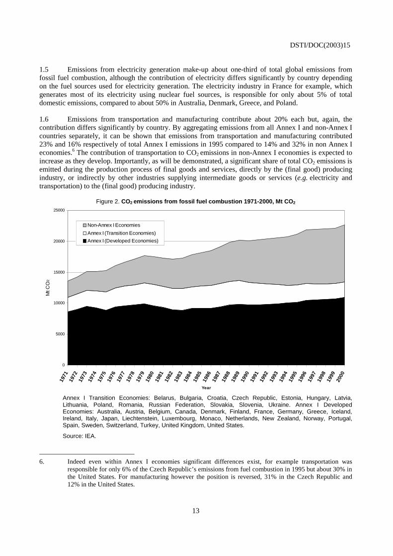
1.5 Emissions from electricity generation make-up about one-third of total global emissions from fossil fuel combustion, although the contribution of electricity differs significantly by country depending on the fuel sources used for electricity generation. The electricity industry in France for example, which generates most of its electricity using nuclear fuel sources, is responsible for only about 5% of total domestic emissions, compared to about 50% in Australia, Denmark, Greece, and Poland.
1.6 Emissions from transportation and manufacturing contribute about 20% each but, again, the contribution differs significantly by country. By aggregating emissions from all Annex I and non-Annex I countries separately, it can be shown that emissions from transportation and manufacturing contributed 23% and 16% respectively of total Annex I emissions in 1995 compared to 14% and 32% in non Annex I economies.6 The contribution of transportation to CO2 emissions in non-Annex I economies is expected to increase as they develop. Importantly, as will be demonstrated, a significant share of total CO2 emissions is emitted during the production process of final goods and services, directly by the (final good) producing industry, or indirectly by other industries supplying intermediate goods or services (e.g. electricity and transportation) to the (final good) producing industry.
Figure 2. CO2 emissions from fossil fuel combustion 1971-2000, Mt CO2
0
5000
10000
15000
20000
25000
1971
1972
1973
1974
1975
1976
1977
1978
1979
1980
1981
1982
1983
1984
1985
1986
1987
1988
1989
1990
1991
1992
1993
1994
1995
1996
1997
1998
1999
2000
Year
Mt C
O2
Non-Annex I Economies
Annex I (Transition Economies)
Annex I (Developed Economies)
Annex I Transition Economies: Belarus, Bulgaria, Croatia, Czech Republic, Estonia, Hungary, Latvia, Lithuania, Poland, Romania, Russian Federation, Slovakia, Slovenia, Ukraine. Annex I Developed Economies: Australia, Austria, Belgium, Canada, Denmark, Finland, France, Germany, Greece, Iceland, Ireland, Italy, Japan, Liechtenstein, Luxembourg, Monaco, Netherlands, New Zealand, Norway, Portugal, Spain, Sweden, Switzerland, Turkey, United Kingdom, United States.
Source: IEA.
6. Indeed even within Annex I economies significant differences exist, for example transportation was
responsible for only 6% of the Czech Republic’s emissions from fuel combustion in 1995 but about 30% in the United States. For manufacturing however the position is reversed, 31% in the Czech Republic and 12% in the United States.
DSTI/DOC(2003)15
14
1.7 Annex I countries as a whole have increased CO2 emissions from fossil fuel consumption by just over 1% since 1990. Although this is broadly consistent with the UNFCC (1992) voluntary pledge by major industrialised nations that they would work to reduce or stabilise emissions in 2000 at 1990 levels, this reflects significant reductions in emissions by Annex I transition economies (Figure 2). Indeed, excluding transition economies, emissions in Annex I countries (Annex II parties7) grew by over 10% over the period. However this is significantly less than the growth in emissions from non-Annex I economies, which have increased by nearly 40% over the last decade. This largely reflects the fact that non-Annex I countries are made up of mainly developing economies in the process of increasing industrialisation, leading inevitably to higher CO2 emissions compared to their relatively low recent levels. China’s emissions alone (the world’s second largest producer of CO2 emissions from fossil-fuel combustion) increased by 25% in the last decade, Brazil’s emissions increased by over 20% and India’s emissions increased by nearly 50%.
The Kyoto Protocol and international trade
1.8 The fact that the Kyoto Protocol restricts emissions only in Annex I countries, but not elsewhere, means there is scope for Annex I countries to reduce domestic emissions without adjusting final demand patterns or finding more carbon efficient production methods to respond to these patterns. This is because they can import more of the goods from non-Annex I countries (whether intermediate or final demand) needed to meet final demand, rather than produce them domestically. This may have a negligible impact on global emissions but, as Annex I economies tend to use less carbon intensive production processes than non-Annex I economies, global emissions could well be higher.8
1.9 The concern for policy makers is that by imposing additional costs, such as taxes on fossil fuel use, the Kyoto protocol may inadvertently encourage such outcomes.9 This will work to reinforce the long-term trend of the declining share of manufacturing in developed economies (as they become increasingly service-oriented) which increasingly import the manufactured goods they once produced from non-Annex I countries. For example, between 1995 and 2000, OECD exports to the rest of the world grew by 7% in nominal dollar terms, whereas imports from the rest of the world to the OECD grew by 47%. Detailed trade figures show that imports of goods that require significant energy to produce them are part of this increase in trade. For example, OECD exports of metals to the rest of the world stood at USD 50 billion in 1995, with imports standing at USD 55 billion. By 2000 however OECD exports to the rest of the world fell to USD 40 billion whereas imports rose to USD 62 billion. The rise of China as a key trading partner for many OECD countries is a key factor behind this shift: China’s share of EU, Japanese and US imports rose from 3%, 5% and 3% in 1990 to 6%, 14% and 8% in 2000. In fact, China is now the leading steel producer in the world, see also Annex A, Table A.1, which shows the source country of imports (as a proportion of the total) in ten countries in 1990 and 2000.
1.10 The potential importance of emissions related to the production of goods for export and import is not generally known. No comprehensive data set has yet been developed which would allow trends in CO2
7. Annex II parties: Annex I parties excluding transition economies.
8. This argument has been made by A. Wyckoff & J.M. Roop, The embodiment of carbon in imports of manufactured products, 1994, Energy Policy March 1994; Munskgaard & Pedersen, CO2 Accounts for Open Economies: Producer or Consumer Responsibility, Energy Policy 29, 2001.
9. Academics, government agencies and increasingly businesses have criticised the Protocol because it does not actively encourage economies to increase the production of goods (and so emissions) where their production processes are amongst the least carbon-intensive in the World. Carbon-intensive sectors such as steel and oil production have been singled out. See for example:
http://www.rautaruukki.fi/rr_web/rr_icc.nsf/allByID/B875E4982B1504CEC2256BA400357680 and http://www.ifc.org/ogmc/docs/proceedings/BernardTRAMIER.pdf
DSTI/DOC(2003)15
15
emissions associated with trade flows to be monitored. Furthermore, identifying the influence of incentives arising from the Kyoto Protocol on these emissions and trade flows would require an empirically based behavioural model. Equilibrium models such as the OECD’s GREEN model have attempted to establish the possible size of changes in global (CO2) emissions that might occur in response to policy or price changes, and these have tended to suggest that this was not likely to be significant. However these models require a number of behavioural assumptions that can restrict the confidence with which conclusions can be drawn. Moreover since the GREEN model was developed the world has changed a great deal, in a way that would have been difficult to predict back then: in particular the collapse of centrally planned economies, the increasing importance of China and, especially since the creation of NAFTA, Mexico10, as producers and exporters of manufactured goods.
1.11 This paper uses input-output, bilateral trade, and IEA CO2 emissions’ data to develop data which can serve as a starting point for an empirical assessment of this issue. Such data may also be of wider interest. For example a substantial effort by a range of formal (e.g. UNFCCC, OECD Annex I Experts Group) and informal (e.g. CCAP Future Actions Dialogue, Pew Centre, various NGOs) groups is currently investigating how the international climate change policy regime might change11 for the post-2012 period. One key criterion (among others) being explored is that of “responsibility”, e.g. the so-called “Brazilian Proposal” which seeks to establish responsibility for future mitigation action based on the attribution of historical-to-now emissions to climate change. However the basis of “responsibility” has not yet been established. For Kyoto, the basis is to measure emissions from domestic production, and this could continue to be the basis. An alternative, or complementary basis, could be to use emissions generated in producing goods to satisfy domestic demand, irrespective of where the goods are produced.
1.12 The methodology developed here is explained in general terms in Section 2 and is set out in detail in Annex B. The main results, reported in Section 3, focus on the size of emissions embodied in traded goods for one year (generally during the mid-1990s) in 24 countries. These provide estimates of the importance of these emissions shortly before the Kyoto agreement was signed, i.e. before it began to influence responses to incentives arising from the Protocol. The paper ends with a summary of the main findings in Section 4.
1.13 In the longer term, as a time series of input-output tables is developed, the scope of this analysis can be extended to determine not just the size and importance of these emissions at a fixed point in time but, also, whether the growth in emissions generated by domestic production has decoupled from the growth in emissions generated (whether domestically or abroad) to meet total domestic (final) demand (Annex A provides illustrative estimates of embodied emissions, over a period of five years for ten countries, that reflect the importance of changes in international trade only, assuming all other things are equal; namely that technology used and relative prices have not changed). Moreover the development of a time series and more recent input-output tables (as used in this analysis) can be used as updated inputs into general equilibrium models such as GREEN and GTAP.12
10. Mexico is not an Annex I country. Its share of US imports increased from 6% in 1990 to 11% in 2000.
11. One idea being considered in the context of emission abatement policies is that developing countries progressively take on more stringent obligations as they cross certain thresholds. Criteria typically mentioned as the basis of these thresholds are GHG emissions per capita or per unit of GDP. This also raises the question of equity or responsibility. While it is true that increased production for others' consumption implies increased national wealth and capability to take on more obligations, this increased wealth is likely to be already picked up as a separate direct indicator. The notion of equity therefore can encompass both production and consumption measures. Quite often the debate surrounding domestic consumption versus domestic production measures is hampered due to a lack of data on domestic consumption measures, the framework presented in this paper can be used to inform this debate
12. Global Trade Analysis Project, Purdue University: http://www.gtap.agecon.purdue.edu/
DSTI/DOC(2003)15
16
2. Methodology
2.1 One way of assessing the significance of CO2 emissions embodied (Box 2) in international trade is to measure total direct and indirect CO2 embodied within products used domestically to satisfy total domestic demand (see Box 3), whether imported or produced domestically.
2.2 The approach is to calculate, for each country (A):
(1) CO2 emitted during the domestic production of manufactured goods and embodied within:
(1.a) Manufactured goods and services consumed in country (A), (and exports of services).
(1.b) Exports of manufactured products from country (A).
(2) CO2, emitted (by other countries) during the production of manufactured goods for export to country (A), and embodied within:
(2.a) Manufactured goods and services consumed in country (A) (and exports of
services). (2.b) Exports of manufactured products from country (A).
2.3 In this way it is possible to define the following aggregates for country (A):
• Domestic consumption of CO2 emissions = (1.a) + (2.a)
• Domestic production of CO2 emissions = (1.a) + (1.b).
• Total exports of embodied emissions = (1.b) + (2.b)13
• Total imports of embodied emissions = (2.a) + (2.b)
• Net trade balance in embodied emissions = (1.b) – (2.a)
13. Often referred to as re-exported emissions in the remainder of this report. This includes emissions
embodied in imports that are directly (re) exported with no additional processing and emissions embodied in imports used in the process of producing exports. Note the double accounting nature of imports and exports which both include this emissions component.
DSTI/DOC(2003)15
17
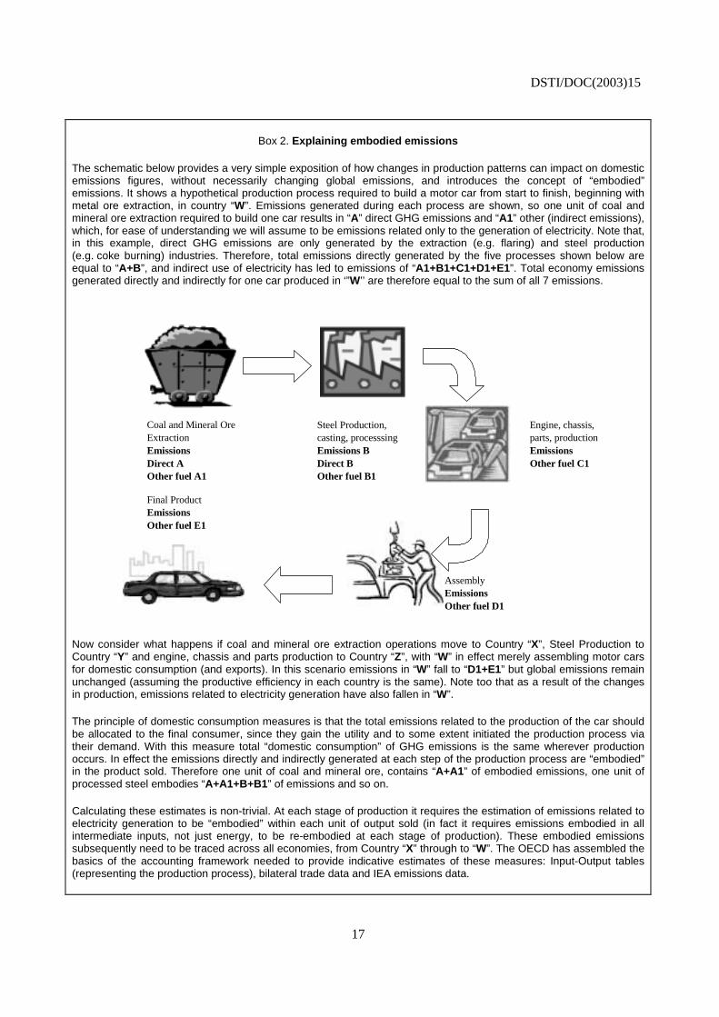
Box 2. Explaining embodied emissions
The schematic below provides a very simple exposition of how changes in production patterns can impact on domestic emissions figures, without necessarily changing global emissions, and introduces the concept of “embodied” emissions. It shows a hypothetical production process required to build a motor car from start to finish, beginning with metal ore extraction, in country “W”. Emissions generated during each process are shown, so one unit of coal and mineral ore extraction required to build one car results in “A” direct GHG emissions and “A1” other (indirect emissions), which, for ease of understanding we will assume to be emissions related only to the generation of electricity. Note that, in this example, direct GHG emissions are only generated by the extraction (e.g. flaring) and steel production (e.g. coke burning) industries. Therefore, total emissions directly generated by the five processes shown below are equal to “A+B”, and indirect use of electricity has led to emissions of “A1+B1+C1+D1+E1”. Total economy emissions generated directly and indirectly for one car produced in ‘”W’’ are therefore equal to the sum of all 7 emissions.
Coal and Mineral Ore ExtractionEmissions Emissions B EmissionsDirect A Direct B Other fuel C1Other fuel A1 Other fuel B1
Final ProductEmissions Other fuel E1
AssemblyEmissionsOther fuel D1
Steel Production, casting, processsing
Engine, chassis, parts, production
Now consider what happens if coal and mineral ore extraction operations move to Country “X”, Steel Production to Country “Y” and engine, chassis and parts production to Country “Z”, with “W” in effect merely assembling motor cars for domestic consumption (and exports). In this scenario emissions in “W” fall to “D1+E1” but global emissions remain unchanged (assuming the productive efficiency in each country is the same). Note too that as a result of the changes in production, emissions related to electricity generation have also fallen in “W”.
The principle of domestic consumption measures is that the total emissions related to the production of the car should be allocated to the final consumer, since they gain the utility and to some extent initiated the production process via their demand. With this measure total “domestic consumption” of GHG emissions is the same wherever production occurs. In effect the emissions directly and indirectly generated at each step of the production process are “embodied” in the product sold. Therefore one unit of coal and mineral ore, contains “A+A1” of embodied emissions, one unit of processed steel embodies “A+A1+B+B1” of emissions and so on.
Calculating these estimates is non-trivial. At each stage of production it requires the estimation of emissions related to electricity generation to be “embodied” within each unit of output sold (in fact it requires emissions embodied in all intermediate inputs, not just energy, to be re-embodied at each stage of production). These embodied emissions subsequently need to be traced across all economies, from Country “X” through to “W”. The OECD has assembled the basics of the accounting framework needed to provide indicative estimates of these measures: Input-Output tables (representing the production process), bilateral trade data and IEA emissions data.
DSTI/DOC(2003)15
18
Box 3. Domestic consumption of embodied emissions
The definition of domestic consumption of embodied emissions used in this context is total emissions (direct and indirect, imported and domestically produced) embodied within household final consumption, general government final consumption, and investment, including changes in inventories. For convenience subsequent references to domestic consumption, in the remainder of this paper, will be based on this definition rather than the more conventional meaning used in the national accounts.
Data sources
2.4 The analysis uses three datasets: input-output tables, international trade flows in manufactured products, and estimates of CO2 emissions from fuel combustion by industry and country. Estimates of CO2 emissions from fuel combustion, embedded within the imports and exports of manufactured goods, agricultural products, mining and quarrying and electricity, are calculated for each country. In this way we are able to show CO2 emissions’ generated by final domestic demand (households, government, investment, inventory changes), reflecting the domestic consumption of embodied emissions, rather than the output of industries.
2.5 A number of studies have attempted to investigate CO2 emissions using this approach,14 most however assume that imported goods are produced in other countries using the same production processes as goods produced domestically. But, at least, for developed economies, this approach is likely to underestimate the significance of trade on global emissions embodied in traded goods. This mainly reflects the fact that goods made in developing economies tend to be more CO2-intensive than the same goods made in developed economies.
2.6 The analysis presented here attempts to overcome any bias by taking technical coefficients from input-output tables (to reflect production processes) in 24 economies15, representing over 80% of world GDP (source World Bank, 2001 data) and CO2 emissions from fuel combustion (source IEA). The analysis begins by comparing the domestic consumption and domestic production of emissions for each country, and the OECD as a whole, providing estimates of the significance of international trade in the context of CO2 emissions and whether they are significant enough to warrant policy consideration.
CO2 emissions from industrial production
2.7 Because bilateral trade data are only presently available for goods and electricity (ISIC 01-40), the main analysis investigates only CO2 emissions used by the industrial production sector (agriculture, mining and quarrying, manufacturing and electricity generation), to produce traded goods, and emissions related to fuel-use for transportation and direct emissions by the service sector are not included in the main results that follow. This omission results in a downward bias of the estimates presented for imports and exports of embodied emissions. (Indicative estimates that include these emissions are presented in Annex B to provide a sensitivity of the nature and size of the bias). Industrial process emissions (not related to
14. Indeed some environmental measures already incorporate this principal, for example the “ecological
footprint” and the Montreal Protocol on Substances that deplete the Ozone Layer (see http://www.unep.org/ozone/montreal.shtml).
15. Australia, Brazil, Canada, China, Czech Republic, Denmark, Finland, France, Germany, Greece, Hungary, India, Italy, Japan, Korea, Netherlands, New Zealand, Norway, Poland, Russia, Spain, Sweden, United Kingdom, United States.
DSTI/DOC(2003)15
19
fossil fuel combustion), which contribute about 3% of total CO2 emissions are also not included. Although relatively insignificant, at the total level, the significance of process emissions across industries and countries may vary considerably, and so some industries will be affected more than others. For example the analysis does not account for carbon dioxide emissions from the production of ammonia in the chemicals industry; process emissions related to cement production; or process emissions from coke used in producing iron and steel. No attempt has been made to quantify these emissions in this report.
Assumptions
2.8 The estimation of emissions embodied in products requires some methodological assumptions and relies heavily on data-quality, particularly in estimating emission factors for those countries where input-output (IO) tables are not presently available. In the main results presented below, conservative assumptions are used to estimate emission factors for the group of countries where country-specific IO tables have not been used. For example, for Mexico and the rest of the world (ROW),16 US emissions factors are used (see Annex B, paragraph B.15, for a complete listing of assumptions used).
2.9 Two variants are presented in Annex B to provide indicative upper and lower bounds on embodied emissions; reflecting the importance of the assumptions used for those countries/regions where no IO data are available. The first, Variant 1, illustrates the size of embodied emissions if less conservative assumptions are used. In this case, for all countries where IO data are not available, Chinese emission factors, as opposed to US, are used. Because, (out of the 24 sampled countries) China is estimated to have amongst the highest emission factors in all industries (see Table 4), Variant 1 estimates can be viewed as upper bounds (excluding embodied transportation, services and other unallocated emissions). The second, Variant 2, uses French emission factors (amongst the lowest of the 24 countries) as opposed to the United States and can be viewed as a lower bound given the heavy reliance of France on the production of electricity through nuclear power.
Time-series of embodied emissions
2.10 Section 3, the main results, presents data for a fixed point in time (in the mid 90s) for each of the 24 countries. In theory it is possible to extend the method used in this section to calculate a time series of domestic consumption. The key assumption in applying input-output analysis to time series data is that the technology in use and relative prices (hence IO coefficients) remain constant over time. For short periods of time this is not an unreasonable assumption, and where only one year is analysed (the same year as the input-output table) it is not necessary at all (and this is largely the case for the analysis shown in Section 3). For longer periods of time however the assumption becomes increasingly weak; particularly if the period of time covers unusual economic events; such as significant changes in relative prices (e.g. oil price shocks); new technology development (e.g. ICT) and, or, political changes (e.g. movement from a centrally planned to a free-market economy).
2.11 Different countries are likely to be affected to varying degrees by these events/processes but it seems likely that economies in transition and economies in the process of industrialisation are likely to have experienced significant changes in their production functions over the last decade. In this context it seems reasonable to assume highly likely that production methods as reflected in IO tables for Brazil, China, Russia, India, Hungary, Poland, and the Czech Republic have changed considerably over the 1990s and that this could affect carbon intensities. Indeed in China, Hungary, Poland and the Czech Republic the 16. ROW reflects all countries except all OECD countries Argentina, Brazil, China, Hong Kong (China), India,
Indonesia, Malaysia, Philippines, Singapore, Taiwan, other OPEC and Russia.
DSTI/DOC(2003)15
20
amount of CO2 emitted per unit of GDP, has fallen over the last decade, in some cases considerably. But in Russia and India they have remained largely unchanged. Whereas in Brazil they have risen by about 20% in the last decade, albeit from a low starting point, (see Annex A). Given its aggregate nature however it is difficult to infer what a change in total economy CO2-intensities means for changes in actual production methods per se. For example, the significant fall in China’s intensities, or rise in Brazil’s, may be partly explained by composition factors, such as increased production of high-tech high-value goods in China’s case.17 Considerable changes have also occurred in developed market economies, for example Denmark’s increasing use of renewable energy sources for electricity, or the United Kingdom’s switch from coal to gas powered generation.
2.12 Nevertheless over a relatively short period of time it may be useful to estimate and investigate outcomes on a “business as usual” assumption, assuming stability in IO coefficients. Looking at total economy CO2 intensities over time provides some indication as to whether economies directly emit more or less CO2 per unit of GDP but it is not possible to ascertain whether changes are the result of changes in the composition of final consumption, production processes, or indeed changes in international trade.
2.13 With a time-series of input-output tables for each country it would be possible to estimate a time-series of emissions embodied in domestic consumption and in turn decompose and identify the factors that drive changes in the domestic production of emissions (and total economy CO2-intensities). Unfortunately a time-series is not currently available for a sufficient number of countries. Nevertheless, it is still possible to construct a time series that can be used to provide tentative indications of trends over time, provided production processes remain largely unchanged, illustrating the importance of changes in the magnitude of trade and consumption explicitly. For example total economy CO2 intensities have fallen by about 15% in the United States since 1990 but concurrent with this is strong growth in the service sector and a significant increase in imports of manufactured goods that may explain at least part of this reduction; and so production processes have probably changed by less than implied by the 15% figure.
2.14 Annex A shows estimates of domestic production and domestic consumption of emissions on this basis, for ten countries for a period of five years, centred around each country’s input-output year (e.g. for Canada, where the IO tables is for 1997, changes in the emissions embodied in domestic consumption are estimated for the period 1995 to 1999). Because in a number of countries, (e.g. Denmark, United Kingdom), significant changes in electricity generation have occurred (coal to wind in Denmark, and coal to gas in the United Kingdom), an attempt has been made to model the production function for electricity generation using CO2-intensity factors from the IEA based on changes in CO2 emissions per KWh basis over time.
17. Some studies, e.g. Garbaccio, Ho and Jorgenson “Why has the Energy-Output Ratio Fallen in China” The
Energy Journal, Vol 20, No3, 1999, which focused on the fall in intensities for the 1987-1992 period, suggest that much of the change in China’s Energy-Output ratio was due to technical changes, although other studies (e.g. Smil, “China’s Energy”, Washington DC, Office of Technology Assessment, Report prepared for the US Congress) have suggested that structural changes have been the dominant factor. More recent studies, e.g. Sinton and Fridley, “What goes up: Recent Trends in China’s Energy consumption”, Energy Policy, March 2000, attribute the fall to a number of factors, including both structural and efficiency changes.
DSTI/DOC(2003)15
21
3. Main results
Summary
3.1 Table 3 below summarises the main results.18 It shows that emissions generated to satisfy domestic demand (domestic consumption of embodied emissions) in OECD economies amounted to over 12Gt CO2 in 1995,19 over 0.5Gt CO2 higher than emissions generated by production, equivalent to 2.5% of global emissions, (and about 5% of OECD emissions). To put this figure into perspective (2.5%) only six countries in the world directly emitted more emissions in 1995, the United States, China, Russia, Japan, Germany and India, (see Table 3). Another way to get a sense of perspective on the magnitude of this figure is to compare it to the Kyoto objective of a 5% reduction in Annex I emissions by 2008-12. Most of the difference between domestic consumption and domestic production of emissions difference can be attributed to the United States, Japan, Germany, France and Italy.
Table 3. CO2 emissions from fossil fuel combustion
Country Year Emissions % of world
(1995)
Domestic production
Mt CO2
Exports (+ re-exports)
Mt CO2
Imports Mt CO2
Domestic consumption
Mt CO2
Difference Mt CO2
Difference % of
domestic production
Australia 1995 1.3 279 47 31 263 16 5.7 Canada 1997 2.2 493 155 101 439 54 10.9 Czech Republic 1995 0.6 126 44 19 100 25 20.1 Denmark 1997 0.3 58 22 21 57 1 1.3 Finland 1995 0.3 56 25 23 54 2 4.3 France 1995 1.7 355 86 139 408 -54 -15.1 Germany 1995 4.1 866 193 254 927 -61 -7.1 Greece 1994 0.3 73 10 13 76 -3 -3.6 Hungary 1998 0.3 57 16 16 57 0 0.1 Italy 1992 2.0 398 60 107 445 -47 -11.9 Japan 1995 5.2 1100 102 289 1287 -187 -17.0 Korea 1995 1.8 364 75 113 402 -38 -10.4 Netherlands 1995 0.8 174 97 77 155 20 11.2 New Zealand 1996 0.1 25 6 9 27 -2 -8.7 Norway 1997 0.2 35 20 19 34 1 3.3 Poland 1995 1.6 328 62 20 286 42 12.7 Spain 1995 1.1 235 45 62 252 -17 -7.2 Sweden 1998 0.3 53 23 30 60 -7 -13.5 United Kingdom 1995 2.5 536 110 123 549 -13 -2.4 United States 1997 24.2 5421 289 552 5684 -263 -4.9 Other OECD 1995 3.9 814 243 284 856 -41 -5.1 Brazil 1996 1.1 258 24 32 266 -8 -3.0 China 1997 14.1 3068 463 102 2708 360 11.7 India 1993 3.7 672 74 24 623 50 7.4 Russia 1998 7.5 1440 256 24 1208 232 16.1
Total OECD 17 1995 54.4 11474 12025 -552 -4.8 World 1995 100 21096
Source: Emissions data used in “emissions % of World” column and “domestic production Mt CO2”, IEA.
18. Although the IO tables used in this study cover countries responsible for 80% of world GDP and trade, the
assumptions used to estimate production processes in other countries have a significant impact on the estimates. The assumptions used to estimate these production processes are therefore deliberately conservative and so too are the estimates of embodied emissions. Figures B1 and B2 in Annex B illustrate this conservative nature by comparing the estimates presented here with higher and lower bounds.
19. OECD estimates for 1995 assume that technology used and relative prices (and so IO coefficients) in 1995, for Canada, Denmark, Greece, Hungary, Italy. New Zealand, Norway, Sweden, and the United States are the same as in the IO year for each country respectively, e.g. 1992 for Italy, see Annex B.
DSTI/DOC(2003)15
22
3.2 The difference between domestic consumption and domestic production is shown above as a percentage of domestic production to highlight the relative importance of embodied emissions in each country. Despite the fact that domestic production is not an ideal scaling factor, since the carbon-intensity of production processes (in particular electricity) varies across countries, and so countries with relatively carbon-free electricity tend to have relatively high percentages, it is arguably, the best scale-factor available. Gross flows of emissions embodied in exports and imports are shown in Figures 3 and 4 below, also as a proportion of total domestic production of emissions.
Figure 3. Emissions embodied in imported goods – percentage of domestic production
0
10
20
30
40
50
60
Aus
tral
iaC
anad
aC
zech
Rep
ublic
Den
mar
kFi
nlan
dFr
ance
Ger
man
yG
reec
eH
unga
ry
Italy
Japa
nK
orea
Net
herl
ands
New
Zea
land
Nor
way
Pol
and
Spa
inS
wed
enU
nite
d K
ingd
omU
nite
d S
tate
sB
razi
lC
hina
Indi
aR
ussi
a
%
Figure 4. Emissions embodied in exported goods – percentage of domestic production
0
10
20
30
40
50
60
Aus
tral
iaC
anad
aC
zech
Rep
ublic
Den
mar
kFi
nlan
dFr
ance
Ger
man
yG
reec
eH
unga
ry
Italy
Japa
nK
orea
Net
herl
ands
New
Zea
land
Nor
way
Pol
and
Spa
inS
wed
enU
nite
d K
ingd
omU
nite
d St
ates
Bra
zil
Chi
na
Indi
aR
ussi
a
%
DSTI/DOC(2003)15
23
Main features
3.3 Figures 3 and 4 illustrate that emissions embodied in (gross) trade flows in OECD economies are usually above 10% of domestic production, and often above 20%. Indeed for Denmark, Finland, France, the Netherlands, Korea, New Zealand, Norway and Sweden, emissions embodied in imports are over 30% of domestic production. Therefore relatively small changes in response to changed competitive conditions or relative prices could imply significant changes to the net balances.
3.4 The OECD, as a whole, had a (negative) trade balance in emissions equivalent to 5% of domestic production, (comparable to the Kyoto 5% reduction objective). The United States, Japan, France, Italy and Korea more than accounted for this, whilst China and Russia more than accounted for the counterpart transfers.
3.5 Moreover, as the OECD’s trade balance (in cash terms) has deteriorated since 1995 (going from a broad balance in 1995 to a USD 340 billion deficit in 2000), so too, is it likely that the trade balance in emissions has also deteriorated, although by how much depends on changes made in the carbon-intensity of production processes over this period. To put this into perspective the combined gross domestic product of the Czech Republic, Hungary, Poland and the Slovak Republic was less then USD 300 billion in 2000 and their combined CO2 emissions from fossil-fuel combustion were more than 0.5Gt CO2; nearly 2.5% of global emissions in 2000 (IEA), (see Annex A, which provides indicative estimates of changes in embodied emissions for ten countries assuming no change in the carbon-intensity of industries, except electricity).
3.6 Figure 5 below illustrates the net position between emissions embodied in imports and exports as a percentage of domestic production (equivalent to the final column in Table 3). It shows that for, many countries, the net position is often +/-10% of domestic production.
Figure 5. Trade balance in CO2 emissions – percentage of domestic production
Canada
DenmarkFinland
FranceGermany
GreeceHungary
ItalyJapan
KoreaNetherlands
New ZealandNorway
PolandSpain
SwedenUnited Kingdom
United StatesBrazil
ChinaIndia
Other OECDTotal OECD
Australia
Russia
Czech Republic
-30.00 -25.00 -20.00 -15.00 -10.00 -5.00 0.00 5.00 10.00 15.00 20.00 25.00 30.00
%
DSTI/DOC(2003)15
24
3.7 Countries with relatively carbon-free electricity generating processes and/or trade deficits in goods (in nominal cash terms), tend to feature on the left hand side of Figure 5 (net importers of embodied emissions), whereas countries with relatively carbon-intensive electricity generating processes and/or trade surpluses feature on the right hand side of the chart. For example in France, Japan, Sweden and Brazil relatively little electricity is generated using fossil fuels.
3.8 France, for example, uses nuclear production for over three-quarters of its electricity production, so, its exports have relatively low embodied emissions values but the high negative figure also reflects the fact that trade plays a relatively large part in France’s economy. Note that total imported French emissions in Table 3 are similar to those in the United Kingdom, which has a similar size economy and exposure to international trade. Australia’s positive figure on the other hand reflects the fact that it produces, and exports, relatively high amounts of carbon-intensive goods and imports goods with relatively low carbon requirements from countries with less carbon-intensive production processes. For example in 1995 one sixth of Australian imports of manufactured goods came from Japan, which uses nuclear generation or renewable energy sources for almost half of its electricity production.
3.9 However these general rules of thumb cannot explain the percentages for all countries and other factors play a role. For example, countries on the left-hand side of the chart may simply use less carbon-intensive production processes more generally than those on the right. Or, it may be that countries on the left of the chart tend to specialise in the production (and export) of goods that require less direct fossil-fuel combustion during production, (e.g. hi-tech goods), than the goods they import, e.g. iron and steel.
Emission factors by sector
3.10 One way of establishing whether countries use relatively clean production processes, compared to other countries, is to investigate the amount of emissions embodied in traded goods for final demand per US dollar by industrial product (Table 4). Some care is needed in interpreting these figures however, since rankings are affected by the extent of aggregation and relative prices.
3.11 Preferably, the emission factors would have volume indicators (e.g. tonnes of steel, numbers of televisions) as the basis of the denominator rather than monetary values. However this is very data intensive, since it requires comparing the same products with each other (see also Box B1), for example 32-inch widescreen TVs should not be compared to 14-inch portables using volume indicators. Therefore a high emission factor for a product in one country compared to another does not necessarily imply that the product, or production process, is more carbon-intensive. The comparison requires that an industry in any country produces the same mix of goods as the same industry in another country and charges the same price, and it is difficult to determine this from the data alone. That said, in heterogeneous industry groupings, such as ‘other metal products, machinery and equipment’ (ISIC28-32), it seems unlikely that these conditions will be satisfied. For example steel industry products are extremely varied, ranging from pig-iron products to specialised stainless steel say20 (see Paragraphs B21-33); moreover a tonne of steel produced in Russia is cheaper than a tonne of equivalent steel produced in the United Kingdom, say. 20. To illustrate this point assume that country A produces one tonne of stainless steel worth USD 1 000 by
processing one tonne of imported unprocessed steel from country B worth USD 100, produced, using nuclear electricity and (for simplicity) no other intermediate inputs. Further assume that the unprocessed steel produced in country B resulted in 50Mt of embodied CO2 emissions per tonne produced. The emission factor for steel production in country B, assuming that it only produces unprocessed steel, would be 0.5Mt CO2 per US dollar (50Mt CO2/USD 100). The emission factor for steel production in country A would be 0.05 Mt CO2 per US dollar (50Mt CO2/USD 1 000), assuming that it only produces stainless steel. And so, although the emission factor in country B is ten times higher than that in country A, one cannot conclude that country A has a cleaner production process than country B.
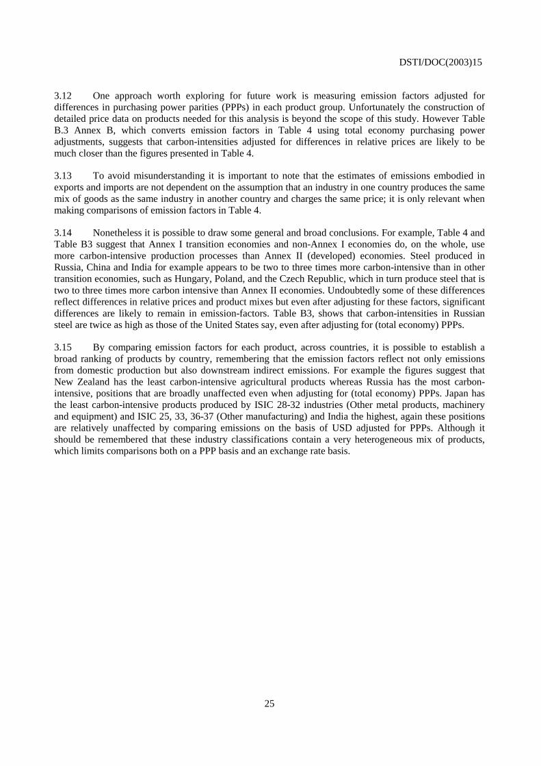
DSTI/DOC(2003)15
25
3.12 One approach worth exploring for future work is measuring emission factors adjusted for differences in purchasing power parities (PPPs) in each product group. Unfortunately the construction of detailed price data on products needed for this analysis is beyond the scope of this study. However Table B.3 Annex B, which converts emission factors in Table 4 using total economy purchasing power adjustments, suggests that carbon-intensities adjusted for differences in relative prices are likely to be much closer than the figures presented in Table 4.
3.13 To avoid misunderstanding it is important to note that the estimates of emissions embodied in exports and imports are not dependent on the assumption that an industry in one country produces the same mix of goods as the same industry in another country and charges the same price; it is only relevant when making comparisons of emission factors in Table 4.
3.14 Nonetheless it is possible to draw some general and broad conclusions. For example, Table 4 and Table B3 suggest that Annex I transition economies and non-Annex I economies do, on the whole, use more carbon-intensive production processes than Annex II (developed) economies. Steel produced in Russia, China and India for example appears to be two to three times more carbon-intensive than in other transition economies, such as Hungary, Poland, and the Czech Republic, which in turn produce steel that is two to three times more carbon intensive than Annex II economies. Undoubtedly some of these differences reflect differences in relative prices and product mixes but even after adjusting for these factors, significant differences are likely to remain in emission-factors. Table B3, shows that carbon-intensities in Russian steel are twice as high as those of the United States say, even after adjusting for (total economy) PPPs.
3.15 By comparing emission factors for each product, across countries, it is possible to establish a broad ranking of products by country, remembering that the emission factors reflect not only emissions from domestic production but also downstream indirect emissions. For example the figures suggest that New Zealand has the least carbon-intensive agricultural products whereas Russia has the most carbon-intensive, positions that are broadly unaffected even when adjusting for (total economy) PPPs. Japan has the least carbon-intensive products produced by ISIC 28-32 industries (Other metal products, machinery and equipment) and ISIC 25, 33, 36-37 (Other manufacturing) and India the highest, again these positions are relatively unaffected by comparing emissions on the basis of USD adjusted for PPPs. Although it should be remembered that these industry classifications contain a very heterogeneous mix of products, which limits comparisons both on a PPP basis and an exchange rate basis.
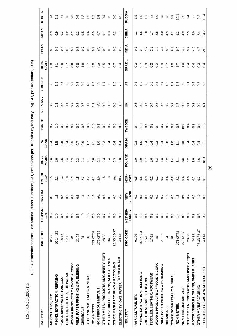
DST
I/D
OC
(200
3)15
26
Tab
le 4
. Em
issi
on
fac
tors
– e
mb
od
ied
(d
irec
t +
ind
irec
t) C
O2
emis
sio
ns
per
US
do
llar
by
ind
ust
ry –
Kg
CO
2 p
er U
S d
olla
r (1
995)
IND
UST
RY
IS
IC C
OD
E
AU
STR
A-
LIA
C
AN
AD
A
CZ
EC
H
RE
P
DE
N-
MA
RK
F
IN-
LA
ND
F
RA
NC
E
GE
RM
AN
Y
GR
EE
CE
H
UN
-G
AR
Y
ITA
LY
JA
PA
N
KO
RE
A
AG
RIC
UL
TU
RE
, ET
C
01-0
5 0.
6 0.
7 1.
5 0.
6 0.
4 0.
2 0.
3 0.
5 0.
9 0.
3 0.
3 0.
4
MIN
ING
, EX
TR
AC
TIO
N, R
EF
ININ
G
10-1
4, 2
3 1.
0 1.
8 2.
1 1.
0 1.
5 1.
0 1.
1 1.
9 3.
1 0.
6 0.
9 1.
1
FO
OD
, BE
VE
RA
GE
S, T
OB
AC
CO
15
-16
0.6
0.4
1.3
0.5
0.5
0.2
0.3
0.5
0.9
0.3
0.2
0.4
TE
XT
ILE
S, L
EA
TH
ER
, FO
OTW
EA
R
17-1
9 0.
5 0.
3 1.
3 0.
4 0.
4 0.
2 0.
4 0.
5 0.
7 0.
3 0.
2 0.
6
WO
OD
& P
RO
DU
CT
S O
F W
OO
D &
CO
RK
20
0.
5 0.
5 1.
3 0.
3 0.
5 0.
2 0.
2 0.
7 0.
9 0.
2 0.
2 0.
5
PU
LP
, PA
PE
R P
RIN
TIN
G &
PU
BL
ISH
ING
21
-22
0.5
0.8
1.5
0.2
0.7
0.2
0.3
0.8
0.8
0.3
0.2
0.6
CH
EM
ICA
LS
24
1.
0 1.
6 2.
2 0.
4 0.
9 0.
5 0.
6 0.
9 1.
8 0.
7 0.
5 1.
3
OT
HE
R N
ON
-ME
TA
LL
IC M
INE
RA
L
26
1.6
1.2
3.2
1.1
1.7
0.6
0.7
4.3
2.7
0.8
0.6
1.5
IRO
N &
ST
EE
L
271+
2731
2.
3 1.
6 4.
1 0.
8 2.
1 1.
5 1.
1 2.
9 3.
0 0.
9 0.
9 1.
2
NO
N-F
ER
RO
US
ME
TA
LS
27
2+27
32
3.0
n/a
2.0
0.3
1.0
0.5
n/a
n/a
n/a
n/a
0.7
1.5
OT
HE
R M
ET
AL
PR
OD
UC
TS
, MA
CH
INE
RY
EQ
PT
28
-32
0.7
0.5
1.5
0.3
0.3
0.2
0.3
1.4
0.5
0.3
0.1
0.4
MO
TO
R V
EH
ICL
ES
, TR
AIN
S, S
HIP
S P
LA
NE
S
34,3
5 0.
6 0.
7 1.
3 0.
4 0.
4 0.
2 0.
3 0.
3 0.
4 0.
3 0.
3 0.
5
OT
HE
R M
AN
UF
AC
TU
RIN
G &
RE
CY
CL
ING
25
,33,
36-3
7 0.
5 0.
7 n/
a 0.
3 0.
4 0.
3 0.
3 1.
0 0.
7 0.
3 0.
2 0.
8
EL
EC
TR
ICIT
Y, G
AS
, WA
TE
R (s
ee A
nn
ex B
, B.3
3)
40-4
1 9.
0 4.
4 10
.7
6.3
4.4
0.5
3.3
7.0
8.4
2.2
1.7
4.9
IND
US
TR
Y
ISIC
CO
DE
N
ET
HE
R-
LA
ND
S
NE
W
Z’L
AN
D
NO
R-
WA
Y
PO
LA
ND
S
PA
IN
SW
ED
EN
U
K
US
B
RA
ZIL
IN
DIA
C
HIN
A
RU
SS
IA
AG
RIC
UL
TU
RE
, ET
C
01-0
5 0.
7 0.
2 0.
5 1.
9 0.
3 0.
4 0.
3 0.
5 0.
3 0.
7 1.
3 1.
9
MIN
ING
, EX
TR
AC
TIO
N, R
EE
FIN
ING
10
-14,
23
1.2
0.9
0.5
3.0
1.6
1.0
0.9
1.9
0.7
2.9
4.5
1.5
FO
OD
, BE
VE
RA
GE
S, T
OB
AC
CO
15
-16
0.4
0.2
0.3
1.7
0.4
0.4
0.4
0.5
0.3
1.2
1.8
1.7
TE
XT
ILE
S, L
EA
TH
ER
, FO
OTW
EA
R
17-1
9 0.
3 0.
3 0.
2 1.
6 0.
4 0.
3 0.
4 0.
5 0.
2 2.
2 1.
7 n/
a
WO
OD
& P
RO
DU
CT
S O
F W
OO
D &
CO
RK
20
0.
2 0.
2 0.
3 2.
2 0.
3 0.
4 0.
3 0.
5 0.
2 1.
0 2.
5 3.
0
PU
LP
, PA
PE
R P
RIN
TIN
G &
PU
BL
ISH
ING
21
-22
0.2
0.2
0.2
1.8
0.4
0.7
0.3
0.4
0.4
3.1
3.0
n/a
CH
EM
ICA
LS
24
0.
8 1.
3 0.
6 3.
2 0.
8 0.
8 0.
7 1.
0 0.
7 3.
9 4.
9 6.
6
OT
HE
R N
ON
-ME
TA
LL
IC M
INE
RA
L
26
0.6
0.2
0.8
4.4
1.0
0.7
0.7
1.3
1.0
6.9
6.1
5.8
IRO
N &
ST
EE
L
271+
2731
1.
4 1.
5 2.
3 5.
1 1.
1 0.
8 1.
6 1.
6 1.
7 9.
2 9.
2 10
.1
NO
N-F
ER
RO
US
ME
TA
LS
27
2+27
32
n/a
n/a
0.6
n/a
n/a
n/a
) 0.
8 0.
9 1.
0 3.
2 4.
9 2.
9
OT
HE
R M
ET
AL
PR
OD
UC
TS
, MA
CH
INE
RY
EQ
PT
28
-32
0.3
0.4
0.3
2.2
0.4
0.4
0.4
0.4
0.4
3.4
2.9
3.4
MO
TO
R V
EH
ICL
ES
, TR
AIN
S, S
HIP
S P
LA
NE
S
34,3
5 0.
3 0.
3 0.
3 2.
0 0.
4 0.
3 0.
3 0.
4 0.
4 4.
9 3.
0 n/
a
OT
HE
R M
AN
UF
AC
TU
RIN
G
25,3
3,36
-37
0.3
1.0
0.2
1.6
0.4
0.4
0.4
0.3
0.3
4.3
2.4
2.2
EL
EC
TR
ICIT
Y, G
AS
& W
AT
ER
SU
PP
LY
40
-41
3.2
0.9
0.1
18.0
3.
1 1.
3 4.
1 6.
8 0.
4 21
.0
24.2
19
.4
DSTI/DOC(2003)15
27
3.16 Table 5 below shows the average emission factor for each country, broken down by the average emission factor for exports of goods and the average emission factor for total domestic final demand (TDFD) of goods (not including electricity and services). It suggests that exports of goods in France, Japan and Italy have the lowest total (embodied) carbon requirements in this group of 24 countries. For Japan and France this mainly reflects their significant use of nuclear power. Russia, China, India and transition economies have the most carbon-intensive production processes, (measured on the basis of Kg CO2 per US dollar). Countries that conduct significant trade with this group of countries also tend to have higher emission factors than might be inferred by looking at their domestic production processes, since the emission factor is based on both direct and indirect emissions (including emissions embodied in imports): explaining why Finland for example, with relatively clean electricity generation, has relatively average emission factors.
3.17 By comparing emission factors of exports and TDFD of goods in each country it is possible to establish that exports of goods in Australia, Canada, the Czech Republic, Greece, Poland, India, China and Russia are significantly more carbon intensive than the goods consumed in the domestic economy. Indeed this is generally the case in most countries, reflecting the fact that the average basket of goods traded internationally tends to be more carbon-intensive than the average basket of goods consumed domestically.
Table 5. Average emission factors per dollar of export and total domestic final demand of goods (TDFD), Kg CO2/USD 1 (1995)
Emission factors Australia Canada Czech Rep Denmark Finland France Germany Greece
Exports 1.1 0.9 2.0 0.5 0.6 0.3 0.4 1.1
TDFD 0.7 0.7 1.5 0.4 0.5 0.3 0.3 0.7
Emission factors Hungary Italy Japan Korea NL NZ Norway Poland Exports 0.9 0.3 0.3 0.6 0.6 0.4 0.5 2.6
TDFD 1.1 0.3 0.2 0.5 0.4 0.3 0.3 1.9
Emission factors Spain Sweden UK US Brazil India China Russia
Exports 0.5 0.6 0.5 0.5 0.5 3.4 2.9 4.1
TDFD 0.5 0.4 0.4 0.6 0.3 1.7 2.1 2.2
Figures for each country are derived by weighting product emission factors by their shares of TDFD and exports in each country’s input-output year, e.g. US, 1997.
3.18 Total embodied emission factors in industries with high direct carbon dioxide emissions, such as iron and steel, chemicals, mining and quarrying, and other non-metallic minerals’ industries are amongst the highest for all industries in nearly all countries. Nevertheless, although smaller, the size of embodied emissions in other products with relatively low direct CO2 emissions, such as motor vehicles, is also significant. Much of this reflects the intermediate consumption of electricity by these industries; about half of all emissions embodied in motor vehicles and machinery reflect embodied emissions from electricity generation, (Table B5, Annex B). In this context, policies aimed at reducing direct emissions from electricity generation, by encouraging more efficient use of electricity, may have a significant impact on the cost structure of industries that have significant electricity needs. Although electricity prices already differ significantly across countries (see Figure B3, Annex B), the evidence suggests that, in some countries at least, relatively high electricity prices have led to a diversification away from industries with high direct electricity requirements. For example, Moriguchi21 ascribes the growth in Japanese imports of refined aluminium from Australia, relative to the growth in bauxite and alumina imports for re-processing in Japan, to the “prohibitively expensive” electricity needed to refine alumina in Japan.
21. Yuichi Moriguchi, Material Flow Data Bank, World Resource Flows around Japan 2003, National Institute
for Environmental studies, Japan.
DSTI/DOC(2003)15
28
Targeting Clean Development Mechanisms
3.19 The combination of data on emissions’ factors and bilateral trade highlights the relationship between emissions embodied in final domestic consumption and emissions generated in exporting partner countries. This information may allow developed countries to target production processes in developing partner economies, providing a mechanism to identify those countries and industries where Clean Development or Joint Implementation Mechanisms might be targeted, particularly by those countries that import significant manufactured goods from them.
3.20 For example it is possible to decompose each emission factor as shown below in Table 4 (and Table B.3) to identify the contribution made by each domestic industry and each imported industrial process, by country of origin. In this way for example, the car industry in country A, say, that imports parts from country B whose steel comes from country C, can estimate the amount of CO2 emitted by steel manufacturers in country C (indirectly) for each car produced in country A. For example if Chinese steel was produced using the same emissions factors as in the United Kingdom, Japan’s total for emissions embodied in imports would decrease by 10%.
3.21 The large difference in emission factors between non-OECD and OECD economies (Table 4 and Table B.3) suggests that the scope for reductions through clean development and joint development mechanisms is considerable.
Decomposing emission factors using own emission factors
3.22 The figures for emissions-factors in Table 4 reflect not only the relative carbon intensity of production processes within countries but the relative importance of trade more generally. One way of isolating the importance of trade is to estimate the size of emissions embodied in imports if the emission factors for imports are assumed to be the same as those used domestically. This calculation assumes that imported products were produced domestically using the domestic production process for that product.
3.23 Most studies that attempt to measure emissions embodied in total domestic final demand tend to adopt this approach. Although, as stated earlier, this is likely to underestimate emissions embodied in imports for developed economies (see paragraph 2.5). Nevertheless taken together with the approach used in Table 3 that calculates emissions embodied in imported products based on the production process that prevails in the country of origin, estimates based on “own-emission” factors help to illustrate two points: (1) the importance of trade generally, and in particular whether exported goods are more CO2-intensive than imports and (2) the importance of the origin of imports.
3.24 Table 6 below compares estimates of emissions embodied in trade, derived using this approach, with those in Table 3 above. Note that differences in exports also occur, reflecting the fact that the emissions embodied in imports used to produce goods for export have also changed. The differences provide insight into how carbon-intensive production processes are in each country relative to the average carbon-intensity for imports (“import emission-intensity”22) for that country.
22. The phrase “import emission-intensity” is used to describe the average emission factor for total imported
goods in any country. This measure will differ for each country since it reflects the mix of products imported by trading partner; which will be different in each country, and so does not reflect the average global value for carbon-intensity more generally. By comparing emissions embodied in imports using a country’s own emission factors and emissions embodied in imports, using estimated emission factors in each exporting country, it is possible to determine if the production processes within countries are more carbon intensive than the “international” average. An alternative approach is to compare emissions embodied in exports using both approaches (a different weighting mechanism). Using this method Australia, Canada, and Greece have emission factors close to their “international” average.
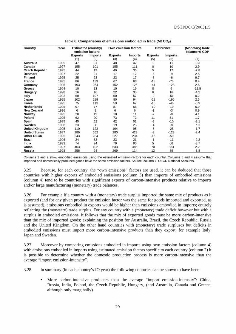
DSTI/DOC(2003)15
29
Table 6. Comparisons of emissions embodied in trade (Mt CO2)
Country Year Estimated (country) emission factors
Own emission factors Difference
Exports Imports Exports Imports Exports Imports
(Monetary) trade balance % GDP
(1) (2) (3) (4) (5) (6) (7) Australia 1995 47 31 48 42 1 11 -0.3 Canada 1997 155 101 155 111 0 10 2.9 Czech Republic 1995 44 19 49 35 5 17 -7.8 Denmark 1997 22 21 17 12 -5 -9 2.5 Finland 1995 25 23 23 17 -3 -6 9.7 France 1995 86 139 67 66 -18 -73 0.4 Germany 1995 193 254 152 126 -41 -128 2.6 Greece 1994 10 13 10 19 0 6 -11.5 Hungary 1998 16 16 22 33 6 16 -4.2 Italy 1992 60 107 50 57 -9 -51 0.2 Japan 1995 102 289 80 94 -22 -196 2.5 Korea 1995 75 113 59 67 -16 -46 -0.9 Netherlands 1995 97 77 87 58 -10 -19 5.9 New Zealand 1996 6 9 6 6 -1 -3 0.9 Norway 1995 20 19 18 11 -2 -8 4.1 Poland 1995 62 20 73 72 11 51 1.7 Spain 1995 45 62 42 52 -3 -10 -3.1 Sweden 1998 23 30 19 23 -4 -8 7.0 United Kingdom 1995 110 123 104 95 -6 -28 -1.7 United States 1997 289 552 280 429 -9 -123 -2.4 Other OECD 1995 243 284 227 234 -16 -50 Brazil 1996 24 32 23 21 -1 -11 -2.2 India 1993 74 24 79 90 5 66 -3.7 China 1997 463 102 533 486 70 384 2.2 Russia 1998 256 24 269 114 12 89 -3.8
Columns 1 and 2 show embodied emissions using the estimated emission-factors for each country. Columns 3 and 4 assume that imported and domestically produced goods have the same emission-factors. Source: column 7, OECD National Accounts.
3.25 Because, for each country, the “own emissions” factors are used, it can be deduced that those countries with higher exports of embodied emissions (column 3) than imports of embodied emissions (column 4) tend to be countries with significant exports of carbon-intensive products relative to imports and/or large manufacturing (monetary) trade balances.
3.26 For example if a country with a (monetary) trade surplus imported the same mix of products as it exported (and for any given product the emission factor was the same for goods imported and exported, as is assumed), emissions embodied in exports would be higher than emissions embodied in imports; entirely reflecting the (monetary) trade surplus. For any country with a (monetary) trade deficit however but with a surplus in embodied emissions, it follows that the mix of exported goods must be more carbon-intensive than the mix of imported goods; explaining the position for Australia, Brazil, the Czech Republic, Russia and the United Kingdom. On the other hand countries with (monetary) trade surpluses but deficits in embodied emissions must import more carbon-intensive products than they export, for example Italy, Japan and Sweden.
3.27 Moreover by comparing emissions embodied in imports using own-emission factors (column 4) with emissions embodied in imports using estimated emission factors specific to each country (column 2) it is possible to determine whether the domestic production process is more carbon-intensive than the average “import emission-intensity”.
3.28 In summary (in each country’s IO year) the following countries can be shown to have been:
• More carbon-intensive producers than the average “import emission-intensity”: China, Russia, India, Poland, the Czech Republic, Hungary, (and Australia, Canada and Greece, although only marginally).
DSTI/DOC(2003)15
30
• Net exporters of “high”23 carbon-intensive goods: Australia, Brazil, the Czech Republic, the United Kingdom, Russia.
• Net Importers of “high” carbon-intensive goods: Japan, Sweden (and Italy, marginally).
• Other countries may (and probably do) fall into the last two categories but this cannot be determined from Table 3 alone.
3.29 The difference between the two measures for calculating domestic consumption of embodied emissions also illustrates the likely impact on global emissions of a substitution of one unit of domestic production with one unit of imports. In 14 of the 20 OECD economies shown above, global emissions are likely to rise if domestic production is replaced with imports, all other things being equal. Of the other six, substitution changes in the Czech Republic, Poland and Hungary are likely to lead to decreases in global emissions and in Australia, Canada and Greece little difference is expected.24
3.30 It is difficult to provide indications of the potential size of substitution effects, since a number of assumptions are needed. However it is clear that if developing economies continue to use more carbon-intensive production processes than developed economies the substitution of domestic production by developed economies with imports from developing economies will lead to increases in global emissions. The development of data, in particular the accumulation of a time-series, provides a starting point for work to assess the size of these effects.
3.31 The role of Chinese exports in this analysis, (and to a lesser but still significant extent Russia,) explain a great deal of the OECD’s trade balance in embodied emissions. Moreover trade between China and the OECD has increased rapidly over the last ten years (and looks set to continue), if this trend continues, the OECD (negative) trade balance in emissions is likely to grow, particularly if Russia and India also increase their market share of OECD economies; which currently remain at relatively low levels. For example in 2000 India was responsible for less than 1% of total imports into the United States, an increase of 0.25 of a per cent from 1990. That said, growth in embodied emissions through increased imports will be offset by reductions coming through from technological advances in the production processes in these countries (see Annex A).
23. High carbon-intensive goods refer to those goods with high emission factors, see Table 4.
24. For all countries this assumes that increases in imported goods have proportionally the same product mix and are sourced proportionally from the same countries as in the relevant IO year in each country. It also assumes that USD 1 of imported goods replaces the same volume of USD 1 domestically produced goods, which is not necessarily (rarely) the case, and no changes in technology used or relative prices.
DSTI/DOC(2003)15
31
4. Summary of main findings
4.1 This analysis has concentrated on emissions embodied in goods only, and not services, such as transportation, (although tentative estimates of these flows are included in Annex B). Moreover the approach used has been deliberately conservative so as to minimise the risk of exaggerating the estimated size of emissions embodied in goods. In addition, no attempt has been made to embody emissions related to the capital services provided by investment in factories, machinery etc into goods purchased by households or produced for export. Nonetheless, despite the conservative approach used, and the fact that emissions embodied in services, e.g. transportation, have not been included, the estimates suggest that the size of CO2 emissions embodied in gross flows of imports and exports is significant, both in relative terms and absolute terms. For example, for Sweden, emissions embodied in imports and exports are equivalent to about 50% of its total domestic production of emissions. And emissions embodied in imports to the United States represent 2.5% of global CO2 emissions from fossil fuel combustion.
4.2 Moreover, the net flows of emissions embodied in trade point to significant net imports of embodied emissions in the OECD as a whole, and for many OECD countries separately. For example, estimates of net imports of embodied emissions in the US in 1997 are roughly equal to the entire emissions from domestic production in Australia, Brazil or Spain. For the OECD, as a whole, estimates of emissions embodied in net imports were equivalent to 2.5% of global emissions in 1995, or 5% of OECD emissions
4.3 The counterpart of OECD net imports is net exports in non-OECD economies; net exports of embodied emissions in China and Russia alone are about the same as net imports in the OECD in 1995. This reflects not only OECD trade deficits in goods with these countries, particularly carbon-intensive goods, but also the fact that production processes in non-OECD economies are, in general, more carbon-intensive. Indeed in sectors sensitive to carbon dioxide-abatement policies, such as iron and steel production, carbon-intensities in non-OECD economies are significantly higher
4.4 Emission intensities do change however, and, certainly for China, these appear to show significant falls (see Annex A). However, part of this reduction may reflect a shift to high-tech high-value production and this may, in turn, open up markets for low-tech low-value goods in other economies; where production processes may continue to be relatively carbon-intensive. In this context the potential impact of India and Russia, with relatively high carbon-intensities, is significant. India has not yet emerged as a big player in an international trade context and Russia’s trade with developed (OECD) economies may grow significantly from its relatively low current levels. However not all non-Annex I economies have high carbon-intensities. Brazil, for example, has relatively low carbon-intensities, reflecting its significant use of renewable energy sources in electricity generation.
4.5 On a sectoral basis, the most carbon-intensive industries are electricity, metals, mining, and chemicals. Direct emissions in most other manufacturing industries tend to be negligible in comparison but when indirect emissions are taken into account the contribution to total emissions made by these industries is revealed as significant. For example although direct emissions from motor vehicle production are usually low (negligible), the industry uses significant inputs from carbon-intensive industries, such as metals and electricity. The picture is similar for other electrical and mechanical machinery industries, reflecting the importance of this group of industries in the context of CDMs and JIMs.
DSTI/DOC(2003)15
32
ANNEX A – EMBODIED EMISSIONS FIVE YEAR GROWTH (TENTATIVE ESTIMATES)
A.1 This Annex investigates trends in emissions embodied in trade for ten countries over a five year period centred around the input-output year of each country: Australia, Canada, Denmark, France, Germany, Italy, Japan, Norway, the United Kingdom and the United States, and illustrates growth in embodied emissions over this period, determining the key originating industries and countries, and whether the significance of growth from developing economies is growing.
A.2 These results are included as an Annex to reflect the greater degree of uncertainty in the estimates shown (see Section 2, paragraphs 2.10-2.12). A number of assumptions are necessarily used and it is not possible to determine the plausibility of these assumptions within the scope of this paper; although they are not thought to detract from the overall conclusion that can be drawn: namely that emissions embodied in international trade are important, growing, and likely to continue to grow. As more data becomes available, this analysis can be replicated relaxing some of the assumptions used in this version.
A.3 The approach used is the same as that in Section 3, and described in Annex B. However, as described in Section 2, assuming no change in technologies in use and relative prices over the 5 year period used restricts the confidence that can be placed on the estimates shown, particularly given the known changes in some key carbon dioxide-emitting sectors, for example electricity generation, and the potentially significant changes in production processes that may have occurred in Transition Economies and China in particular.
A.4 Figure A1 below, which shows direct CO2 emissions per US dollar of GDP, in ten selected countries/regions, over a ten-year period, suggests that in China, at least, (where the ratio has fallen by about a half) production processes have become less carbon-intensive; although it is not so clear-cut for Russia, India and Brazil, or indeed any of the other selected countries. Because of the aggregated nature of GDP however some caution is needed in interpretation, since, it is does not differentiate between changes in industrial production processes (technical change) and increased production of goods that are less carbon-intensive (structural change).
A.5 It is possible to gauge the significance of some of these factors using two or more input-output tables however. In 1997, emissions from United States industrial production (agriculture, mining and quarrying, manufacturing and electricity) amounted to 2 836 Mt CO2. If the same mix of goods purchased in final demand in 1997 was produced using 1990 production techniques it is estimated that emissions from industrial production would have been 2 949 Mt CO2, suggesting that the CO2-intensity of United States industrial production fell by less than 4% over this period.25 Part of this reduction reflects the reduced carbon-intensity of electricity generation; which fell by 2% between 1990 and 1997. Indeed, 1997 emissions would have been 2 909 Mt CO2 if 1990 production processes were used, except for electricity; suggesting that the carbon-intensity of United States industrial production (excluding electricity) fell by
25. Estimates of emissions on this basis are sensitive to the deflators used. The estimates presented here are
central estimates. The range of the reduction in CO2-intensities for industrial production is likely to lie between 2.5 and 5%.
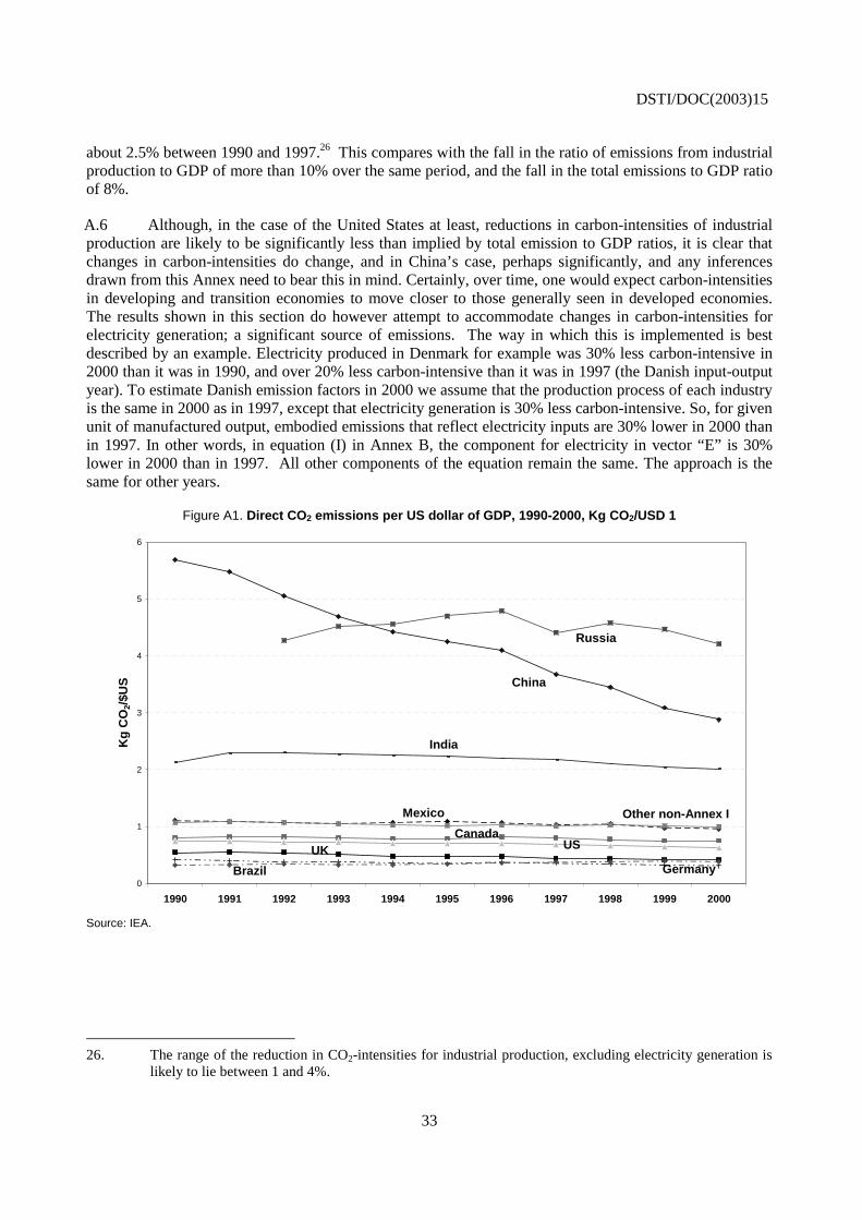
DSTI/DOC(2003)15
33
about 2.5% between 1990 and 1997.26 This compares with the fall in the ratio of emissions from industrial production to GDP of more than 10% over the same period, and the fall in the total emissions to GDP ratio of 8%.
A.6 Although, in the case of the United States at least, reductions in carbon-intensities of industrial production are likely to be significantly less than implied by total emission to GDP ratios, it is clear that changes in carbon-intensities do change, and in China’s case, perhaps significantly, and any inferences drawn from this Annex need to bear this in mind. Certainly, over time, one would expect carbon-intensities in developing and transition economies to move closer to those generally seen in developed economies. The results shown in this section do however attempt to accommodate changes in carbon-intensities for electricity generation; a significant source of emissions. The way in which this is implemented is best described by an example. Electricity produced in Denmark for example was 30% less carbon-intensive in 2000 than it was in 1990, and over 20% less carbon-intensive than it was in 1997 (the Danish input-output year). To estimate Danish emission factors in 2000 we assume that the production process of each industry is the same in 2000 as in 1997, except that electricity generation is 30% less carbon-intensive. So, for given unit of manufactured output, embodied emissions that reflect electricity inputs are 30% lower in 2000 than in 1997. In other words, in equation (I) in Annex B, the component for electricity in vector “E” is 30% lower in 2000 than in 1997. All other components of the equation remain the same. The approach is the same for other years.
Figure A1. Direct CO2 emissions per US dollar of GDP, 1990-2000, Kg CO2/USD 1
China
Russia
India
Mexico
CanadaUSUK
GermanyBrazil
Other non-Annex I
0
1
2
3
4
5
6
1990 1991 1992 1993 1994 1995 1996 1997 1998 1999 2000
Kg
CO
2/$U
S
Source: IEA.
26. The range of the reduction in CO2-intensities for industrial production, excluding electricity generation is
likely to lie between 1 and 4%.
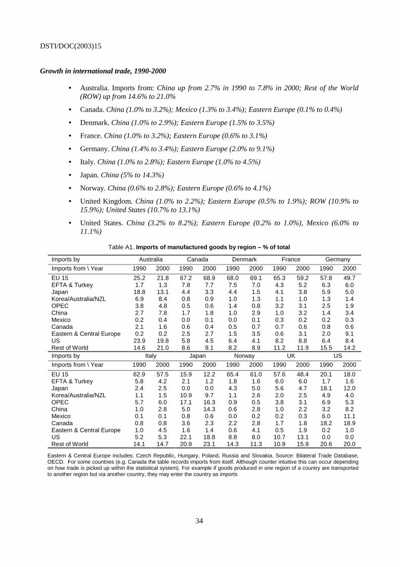
DSTI/DOC(2003)15
34
Growth in international trade, 1990-2000
• Australia. Imports from: China up from 2.7% in 1990 to 7.8% in 2000; Rest of the World (ROW) up from 14.6% to 21.0%
• Canada. China (1.0% to 3.2%); Mexico (1.3% to 3.4%); Eastern Europe (0.1% to 0.4%)
• Denmark. China (1.0% to 2.9%); Eastern Europe (1.5% to 3.5%)
• France. China (1.0% to 3.2%); Eastern Europe (0.6% to 3.1%)
• Germany. China (1.4% to 3.4%); Eastern Europe (2.0% to 9.1%)
• Italy. China (1.0% to 2.8%); Eastern Europe (1.0% to 4.5%)
• Japan. China (5% to 14.3%)
• Norway. China (0.6% to 2.8%); Eastern Europe (0.6% to 4.1%)
• United Kingdom. China (1.0% to 2.2%); Eastern Europe (0.5% to 1.9%); ROW (10.9% to 15.9%); United States (10.7% to 13.1%)
• United States. China (3.2% to 8.2%); Eastern Europe (0.2% to 1.0%), Mexico (6.0% to 11.1%)
Table A1. Imports of manufactured goods by region – % of total
Imports by Australia Canada Denmark France Germany
Imports from \ Year 1990 2000 1990 2000 1990 2000 1990 2000 1990 2000
EU 15 25.2 21.8 67.2 68.9 68.0 69.1 65.3 59.2 57.8 49.7 EFTA & Turkey 1.7 1.3 7.8 7.7 7.5 7.0 4.3 5.2 6.3 6.0 Japan 18.8 13.1 4.4 3.3 4.4 1.5 4.1 3.8 5.9 5.0 Korea/Australia/NZL 6.9 8.4 0.8 0.9 1.0 1.3 1.1 1.0 1.3 1.4 OPEC 3.8 4.8 0.5 0.6 1.4 0.8 3.2 3.1 2.5 1.9 China 2.7 7.8 1.7 1.8 1.0 2.9 1.0 3.2 1.4 3.4 Mexico 0.2 0.4 0.0 0.1 0.0 0.1 0.3 0.2 0.2 0.3 Canada 2.1 1.6 0.6 0.4 0.5 0.7 0.7 0.6 0.8 0.6 Eastern & Central Europe 0.2 0.2 2.5 2.7 1.5 3.5 0.6 3.1 2.0 9.1 US 23.9 19.8 5.8 4.5 6.4 4.1 8.2 8.8 6.4 8.4 Rest of World 14.6 21.0 8.6 9.1 8.2 8.9 11.2 11.9 15.5 14.2 Imports by Italy Japan Norway UK US
Imports from \ Year 1990 2000 1990 2000 1990 2000 1990 2000 1990 2000
EU 15 62.9 57.5 15.9 12.2 65.4 61.0 57.6 48.4 20.1 18.0 EFTA & Turkey 5.8 4.2 2.1 1.2 1.8 1.6 6.0 6.0 1.7 1.6 Japan 2.4 2.5 0.0 0.0 4.3 5.0 5.6 4.7 18.1 12.0 Korea/Australia/NZL 1.1 1.5 10.9 9.7 1.1 2.6 2.0 2.5 4.9 4.0 OPEC 5.7 6.0 17.1 16.3 0.9 0.5 3.8 3.1 6.9 5.3 China 1.0 2.8 5.0 14.3 0.6 2.8 1.0 2.2 3.2 8.2 Mexico 0.1 0.1 0.8 0.6 0.0 0.2 0.2 0.3 6.0 11.1 Canada 0.8 0.8 3.6 2.3 2.2 2.8 1.7 1.8 18.2 18.9 Eastern & Central Europe 1.0 4.5 1.6 1.4 0.6 4.1 0.5 1.9 0.2 1.0 US 5.2 5.3 22.1 18.8 8.8 8.0 10.7 13.1 0.0 0.0 Rest of World 14.1 14.7 20.9 23.1 14.3 11.3 10.9 15.9 20.6 20.0
Eastern & Central Europe includes: Czech Republic, Hungary, Poland, Russia and Slovakia. Source: Bilateral Trade Database, OECD. For some countries (e.g. Canada the table records imports from itself. Although counter intuitive this can occur depending on how trade is picked up within the statistical system). For example if goods produced in one region of a country are transported to another region but via another country, they may enter the country as imports
DSTI/DOC(2003)15
35
Embodied emissions
A.7 Because China has relatively high emission factors (Table 4) the impact of an increase in imports from China on total emissions embodied in imports is considerable. Table A.2 below, which shows the source-country of emissions embodied in imports, confirms this. In the United States, for example, emissions embodied in imported Chinese goods made up about 20% of total emissions embodied in imports in 1995 rising to over one-quarter of imported emissions in 2000, and in Japan, they rose from under 20% of total imported emissions to one-third between 1993 and 1997. Eastern Europe is also a growing source of imported embodied emissions. For example the contribution of Eastern Europe to total imported emissions in Germany rose from 18% in 1993 to over 23% in 1997.
A.8 Although the growth in emissions embodied in imports has been significant in all countries (Figure A2), it is still lower than real constant price growth in imported goods in nearly all countries. This reflects two points: (1) constant price growth measures tend to move ahead of quantity measures if quality changes (improvements) in products occur and so the deflators used in this analysis for manufactured goods (ISIC 28-37) (conservatively) attempt to adjust for these quality changes, measuring quantities and not constant prices27 (see Annex B); and (2) changes in electricity generation in each year for each country have been accounted for, and so if the CO2-intensity of electricity generation reduces over time so too do emission factors (see Annex B). Exports of embodied emissions have also grown strongly, see Figure A3. Note in figure A3 the spike for Denmark in 1996, reflecting its significant electricity exports in that year, and the corresponding rise in imports for Norway in Figure A2.
27. A simple example can be used to illustrate this point. All other things equal the production of a computer,
say, in 1990 is likely to have resulted in about the same amount of (embodied) CO2 emissions as a computer produced in 2000, as the raw materials required for each are broadly the same. Let us assume that each computer embodies X emissions, and that country A produces 100 computers in 1990 for export to country Y at cost USD 1 000 each, and 100 computers in 2000 at cost USD 500 each, again for export to country Y, so the emission factor for USD 1 of computers in 2000 is equal to X/500. In both 1990 and 2000 emissions embodied in computer imports by country Y are the same, 100X. Assume also that the USD 500 computer would have been worth USD 2 000 if available in 1990, the price index for computers in 2000 would record a 75% fall since 1990. So, imports in 1990 (USD 100 000) in 2000 prices using the price index for 2000 quality computers would be equivalent to USD 25 000. Assuming that emissions factors in constant prices are constant over this ten-year period would mean that emissions embodied in imports in 1990 are estimated at 50X, if the emission factors for 2000 are applied, and not 100X as would have been expected. The assumption used in this paper is that embodied emissions per quantity of output are the same. For most products quantities and constant prices move in line with each other but where rapid quality changes occur, so too does a decoupling of these indices.
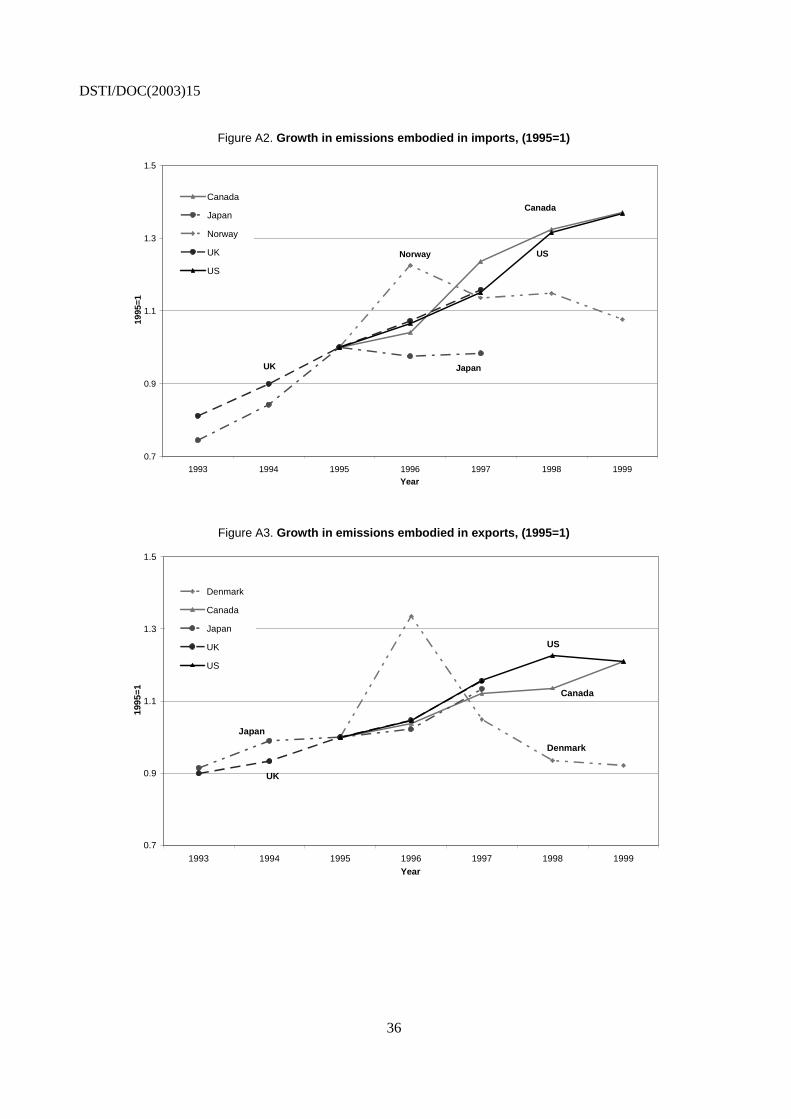
DSTI/DOC(2003)15
36
Figure A2. Growth in emissions embodied in imports, (1995=1)
Canada
Japan
Norway US
UK
0.7
0.9
1.1
1.3
1.5
1993 1994 1995 1996 1997 1998 1999Year
1995
=1
Canada
Japan
Norway
UK
US
Figure A3. Growth in emissions embodied in exports, (1995=1)
Denmark
Canada
Japan
US
UK
0.7
0.9
1.1
1.3
1.5
1993 1994 1995 1996 1997 1998 1999Year
1995
=1
Denmark
Canada
Japan
UK
US
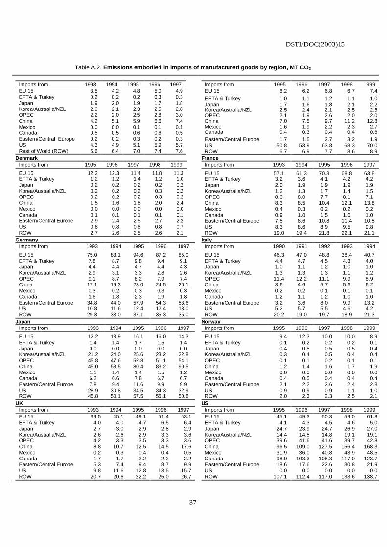
DSTI/DOC(2003)15
37
Table A.2. Emissions embodied in imports of manufactured goods by region, MT CO2
Imports from 1993 1994 1995 1996 1997 EU 15 3.5 4.2 4.8 5.0 4.9 EFTA & Turkey 0.2 0.2 0.2 0.3 0.3 Japan 1.9 2.0 1.9 1.7 1.8 Korea/Australia/NZL 2.0 2.1 2.3 2.5 2.8 OPEC 2.2 2.0 2.5 2.8 3.0 China 4.2 5.1 5.9 6.6 7.4 Mexico 0.0 0.0 0.1 0.1 0.1 Canada 0.5 0.5 0.6 0.6 0.5 Eastern/Central Europe 0.2 0.2 0.3 0.2 0.3 US 4.3 4.9 5.1 5.9 5.7 Rest of World (ROW) 5.6 6.4 7.0 7.4 7.6
Imports from 1995 1996 1997 1998 1999 EU 15 6.2 6.2 6.8 6.7 7.4 EFTA & Turkey 1.0 1.1 1.2 1.1 1.0 Japan 1.7 1.6 1.8 2.1 2.2 Korea/Australia/NZL 2.5 2.4 2.1 2.5 2.5 OPEC 2.1 1.9 2.6 2.0 2.0 China 7.0 7.5 9.7 11.2 12.8 Mexico 1.6 1.9 2.2 2.3 2.7 Canada 0.4 0.3 0.4 0.4 0.6 Eastern/Central Europe 1.7 1.5 2.7 3.2 1.9 US 50.8 53.9 63.8 68.3 70.0 ROW 6.7 6.9 7.7 8.6 8.9
Denmark France Imports from 1995 1996 1997 1998 1999
EU 15 12.2 12.3 11.4 11.8 11.3 EFTA & Turkey 1.2 1.2 1.4 1.2 1.0 Japan 0.2 0.2 0.2 0.2 0.2 Korea/Australia/NZL 0.2 0.2 0.2 0.3 0.2 OPEC 0.2 0.2 0.2 0.3 0.2 China 1.5 1.6 1.8 2.0 2.4 Mexico 0.0 0.0 0.0 0.0 0.0 Canada 0.1 0.1 0.1 0.1 0.1 Eastern/Central Europe 2.9 2.4 2.5 2.7 2.2 US 0.8 0.8 0.8 0.8 0.7 ROW 2.7 2.6 2.5 2.6 2.1
Imports from 1993 1994 1995 1996 1997
EU 15 57.1 61.3 70.3 68.8 63.8 EFTA & Turkey 3.2 3.6 4.1 4.2 4.2 Japan 2.0 1.9 1.9 1.9 1.9 Korea/Australia/NZL 1.2 1.3 1.7 1.4 1.5 OPEC 8.3 8.0 7.7 8.1 7.1 China 8.3 8.5 10.4 12.1 13.8 Mexico 0.4 0.3 0.2 0.2 0.2 Canada 0.9 1.0 1.5 1.0 1.0 Eastern/Central Europe 7.5 8.6 10.8 11.4 10.5 US 8.3 8.6 8.9 9.5 9.8 ROW 19.0 19.4 21.8 22.1 21.1
Germany Italy Imports from 1993 1994 1995 1996 1997
EU 15 75.0 83.1 94.6 87.2 85.0 EFTA & Turkey 7.8 8.7 9.8 9.4 9.1 Japan 4.4 4.4 4.7 4.4 4.3 Korea/Australia/NZL 2.9 3.1 3.3 2.8 2.6 OPEC 9.1 8.7 8.2 7.9 7.4 China 17.1 19.3 23.0 24.5 26.1 Mexico 0.3 0.2 0.3 0.3 0.3 Canada 1.6 1.8 2.3 1.9 1.8 Eastern/Central Europe 34.8 44.0 57.9 54.3 53.6 US 10.8 11.6 12.4 12.4 13.0 ROW 29.3 33.0 37.1 35.3 35.0
Imports from 1990 1991 1992 1993 1994
EU 15 46.3 47.0 48.8 38.4 40.7 EFTA & Turkey 4.4 4.7 4.5 4.3 4.0 Japan 1.0 1.1 1.2 1.0 1.0 Korea/Australia/NZL 1.3 1.3 1.3 1.1 1.2 OPEC 11.4 12.2 11.1 9.9 8.9 China 3.6 4.6 5.7 5.6 6.2 Mexico 0.2 0.2 0.1 0.1 0.1 Canada 1.2 1.1 1.2 1.0 1.0 Eastern/Central Europe 3.2 3.6 8.0 9.9 13.2 US 5.2 5.7 5.5 4.6 4.2 ROW 20.2 19.0 19.7 18.9 21.3
Japan Norway Imports from 1993 1994 1995 1996 1997
EU 15 12.2 13.9 16.1 16.0 14.3 EFTA & Turkey 1.4 1.4 1.7 1.5 1.4 Japan 0.0 0.0 0.0 0.0 0.0 Korea/Australia/NZL 21.2 24.0 25.6 23.2 22.8 OPEC 45.8 47.6 52.8 51.1 54.1 China 45.0 58.5 80.4 83.2 90.5 Mexico 1.1 1.4 1.4 1.5 1.2 Canada 6.2 6.6 7.8 6.7 6.7 Eastern/Central Europe 7.8 9.4 11.6 9.9 9.9 US 28.9 30.8 34.5 34.3 32.9 ROW 45.8 50.1 57.5 55.1 50.8
Imports from 1995 1996 1997 1998 1999
EU 15 9.4 12.3 10.0 10.0 8.9 EFTA & Turkey 0.1 0.2 0.2 0.2 0.1 Japan 0.4 0.5 0.5 0.5 0.4 Korea/Australia/NZL 0.3 0.4 0.5 0.4 0.4 OPEC 0.1 0.1 0.2 0.1 0.1 China 1.2 1.4 1.6 1.7 1.9 Mexico 0.0 0.0 0.0 0.0 0.0 Canada 0.4 0.5 0.4 0.4 0.4 Eastern/Central Europe 2.1 2.2 2.6 2.4 2.8 US 0.9 0.9 0.9 1.1 1.0 ROW 2.0 2.3 2.3 2.5 2.1
UK US Imports from 1993 1994 1995 1996 1997 EU 15 39.5 45.1 49.1 51.4 53.1 EFTA & Turkey 4.0 4.0 4.7 6.5 6.4 Japan 2.7 3.0 2.9 2.8 2.9 Korea/Australia/NZL 2.6 2.6 2.9 3.3 3.6 OPEC 4.2 3.3 3.5 3.3 3.6 China 8.8 10.7 12.5 14.5 17.6 Mexico 0.2 0.3 0.4 0.4 0.5 Canada 1.7 1.7 2.2 2.2 2.2 Eastern/Central Europe 5.3 7.4 9.4 8.7 9.9 US 9.8 11.6 12.8 13.5 15.7 ROW 20.7 20.6 22.2 25.0 26.7
Imports from 1995 1996 1997 1998 1999 EU 15 45.1 49.3 50.3 59.0 61.8 EFTA & Turkey 4.1 4.3 4.5 4.6 5.0 Japan 24.7 23.9 24.7 26.9 27.0 Korea/Australia/NZL 14.4 14.5 14.8 19.1 19.1 OPEC 39.6 41.6 41.6 39.7 42.8 China 96.5 109.0 127.5 156.4 168.3 Mexico 31.9 36.0 40.8 43.9 48.5 Canada 98.0 103.3 108.3 117.0 123.7 Eastern/Central Europe 18.6 17.6 22.6 30.8 21.9 US 0.0 0.0 0.0 0.0 0.0 ROW 107.1 112.4 117.0 133.6 138.7
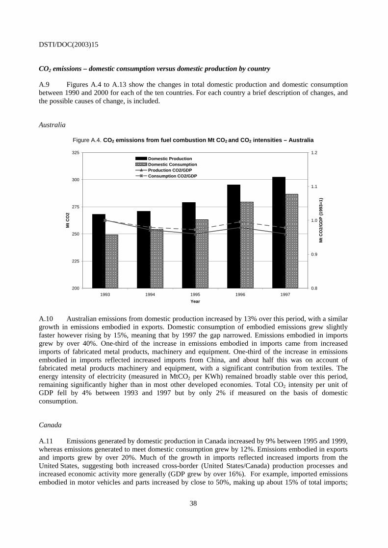
DSTI/DOC(2003)15
38
CO2 emissions – domestic consumption versus domestic production by country
A.9 Figures A.4 to A.13 show the changes in total domestic production and domestic consumption between 1990 and 2000 for each of the ten countries. For each country a brief description of changes, and the possible causes of change, is included.
Australia
Figure A.4. CO2 emissions from fuel combustion Mt CO2 and CO2 intensities – Australia
200
225
250
275
300
325
1993 1994 1995 1996 1997
Year
Mt
CO
2
0.8
0.9
1.0
1.1
1.2
Mt
CO
2/G
DP
(19
93=1
)
Domestic ProductionDomestic ConsumptionProduction CO2/GDPConsumption CO2/GDP
A.10 Australian emissions from domestic production increased by 13% over this period, with a similar growth in emissions embodied in exports. Domestic consumption of embodied emissions grew slightly faster however rising by 15%, meaning that by 1997 the gap narrowed. Emissions embodied in imports grew by over 40%. One-third of the increase in emissions embodied in imports came from increased imports of fabricated metal products, machinery and equipment. One-third of the increase in emissions embodied in imports reflected increased imports from China, and about half this was on account of fabricated metal products machinery and equipment, with a significant contribution from textiles. The energy intensity of electricity (measured in MtCO2 per KWh) remained broadly stable over this period, remaining significantly higher than in most other developed economies. Total CO2 intensity per unit of GDP fell by 4% between 1993 and 1997 but by only 2% if measured on the basis of domestic consumption.
Canada
A.11 Emissions generated by domestic production in Canada increased by 9% between 1995 and 1999, whereas emissions generated to meet domestic consumption grew by 12%. Emissions embodied in exports and imports grew by over 20%. Much of the growth in imports reflected increased imports from the United States, suggesting both increased cross-border (United States/Canada) production processes and increased economic activity more generally (GDP grew by over 16%). For example, imported emissions embodied in motor vehicles and parts increased by close to 50%, making up about 15% of total imports;
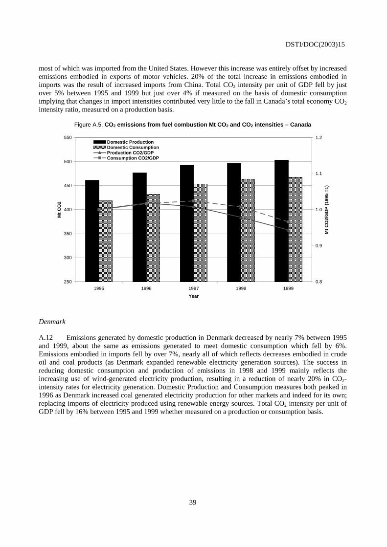
DSTI/DOC(2003)15
39
most of which was imported from the United States. However this increase was entirely offset by increased emissions embodied in exports of motor vehicles. 20% of the total increase in emissions embodied in imports was the result of increased imports from China. Total CO2 intensity per unit of GDP fell by just over 5% between 1995 and 1999 but just over 4% if measured on the basis of domestic consumption implying that changes in import intensities contributed very little to the fall in Canada’s total economy CO2
intensity ratio, measured on a production basis.
Figure A.5. CO2 emissions from fuel combustion Mt CO2 and CO2 intensities – Canada
250
300
350
400
450
500
550
1995 1996 1997 1998 1999
Year
Mt
CO
2
0.8
0.9
1.0
1.1
1.2
Mt
CO
2/G
DP
(19
95 =
1)
Domestic ProductionDomestic ConsumptionProduction CO2/GDPConsumption CO2/GDP
Denmark
A.12 Emissions generated by domestic production in Denmark decreased by nearly 7% between 1995 and 1999, about the same as emissions generated to meet domestic consumption which fell by 6%. Emissions embodied in imports fell by over 7%, nearly all of which reflects decreases embodied in crude oil and coal products (as Denmark expanded renewable electricity generation sources). The success in reducing domestic consumption and production of emissions in 1998 and 1999 mainly reflects the increasing use of wind-generated electricity production, resulting in a reduction of nearly 20% in CO2- intensity rates for electricity generation. Domestic Production and Consumption measures both peaked in 1996 as Denmark increased coal generated electricity production for other markets and indeed for its own; replacing imports of electricity produced using renewable energy sources. Total CO2 intensity per unit of GDP fell by 16% between 1995 and 1999 whether measured on a production or consumption basis.
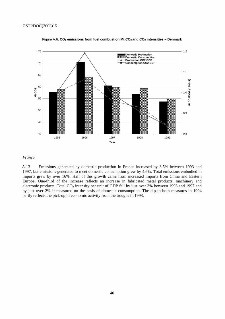
DSTI/DOC(2003)15
40
Figure A.6. CO2 emissions from fuel combustion Mt CO2 and CO2 intensities – Denmark
40
45
50
55
60
65
70
75
1995 1996 1997 1998 1999
Year
Mt
CO
2
0.8
0.9
1.0
1.1
1.2
Mt
CO
2/G
DP
(19
95=1
)
Domestic Production Domestic ConsumptionProduction CO2/GDPConsumption CO2/GDP
France
A.13 Emissions generated by domestic production in France increased by 3.5% between 1993 and 1997, but emissions generated to meet domestic consumption grew by 4.6%. Total emissions embodied in imports grew by over 16%. Half of this growth came from increased imports from China and Eastern Europe. One-third of the increase reflects an increase in fabricated metal products, machinery and electronic products. Total CO2 intensity per unit of GDP fell by just over 3% between 1993 and 1997 and by just over 2% if measured on the basis of domestic consumption. The dip in both measures in 1994 partly reflects the pick-up in economic activity from the troughs in 1993.
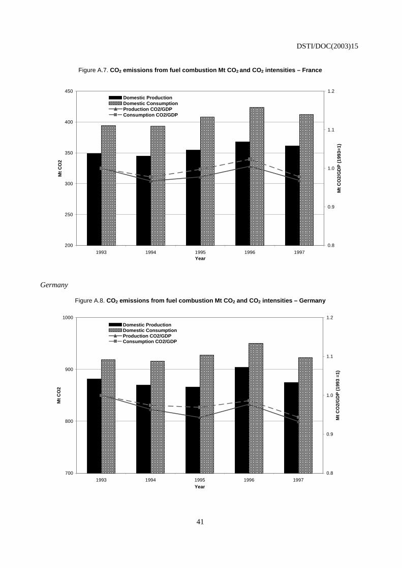
DSTI/DOC(2003)15
41
Figure A.7. CO2 emissions from fuel combustion Mt CO2 and CO2 intensities – France
200
250
300
350
400
450
1993 1994 1995 1996 1997Year
Mt
CO
2
0.8
0.9
1.0
1.1
1.2
Mt
CO
2/G
DP
(19
93=1
)
Domestic ProductionDomestic ConsumptionProduction CO2/GDPConsumption CO2/GDP
Germany
Figure A.8. CO2 emissions from fuel combustion Mt CO2 and CO2 intensities – Germany
700
800
900
1000
1993 1994 1995 1996 1997Year
Mt
CO
2
0.8
0.9
1.0
1.1
1.2
Mt
CO
2/G
DP
(19
93 =
1)
Domestic ProductionDomestic ConsumptionProduction CO2/GDPConsumption CO2/GDP
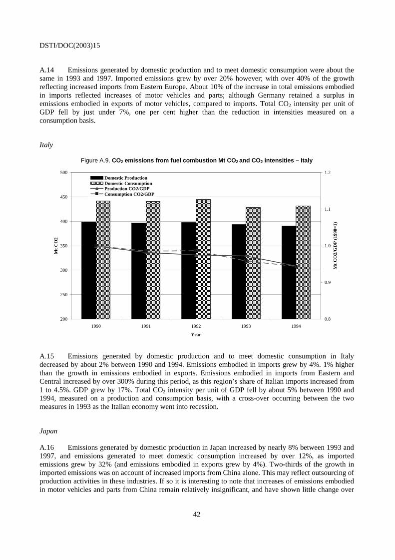
DSTI/DOC(2003)15
42
A.14 Emissions generated by domestic production and to meet domestic consumption were about the same in 1993 and 1997. Imported emissions grew by over 20% however; with over 40% of the growth reflecting increased imports from Eastern Europe. About 10% of the increase in total emissions embodied in imports reflected increases of motor vehicles and parts; although Germany retained a surplus in emissions embodied in exports of motor vehicles, compared to imports. Total CO2 intensity per unit of GDP fell by just under 7%, one per cent higher than the reduction in intensities measured on a consumption basis.
Italy
Figure A.9. CO2 emissions from fuel combustion Mt CO2 and CO2 intensities – Italy
200
250
300
350
400
450
500
1990 1991 1992 1993 1994
Year
Mt
CO
2
0.8
0.9
1.0
1.1
1.2
Mt
CO
2/G
DP
(19
90=1
)
Domestic ProductionDomestic ConsumptionProduction CO2/GDPConsumption CO2/GDP
A.15 Emissions generated by domestic production and to meet domestic consumption in Italy decreased by about 2% between 1990 and 1994. Emissions embodied in imports grew by 4%. 1% higher than the growth in emissions embodied in exports. Emissions embodied in imports from Eastern and Central increased by over 300% during this period, as this region’s share of Italian imports increased from 1 to 4.5%. GDP grew by 17%. Total CO2 intensity per unit of GDP fell by about 5% between 1990 and 1994, measured on a production and consumption basis, with a cross-over occurring between the two measures in 1993 as the Italian economy went into recession.
Japan
A.16 Emissions generated by domestic production in Japan increased by nearly 8% between 1993 and 1997, and emissions generated to meet domestic consumption increased by over 12%, as imported emissions grew by 32% (and emissions embodied in exports grew by 4%). Two-thirds of the growth in imported emissions was on account of increased imports from China alone. This may reflect outsourcing of production activities in these industries. If so it is interesting to note that increases of emissions embodied in motor vehicles and parts from China remain relatively insignificant, and have shown little change over
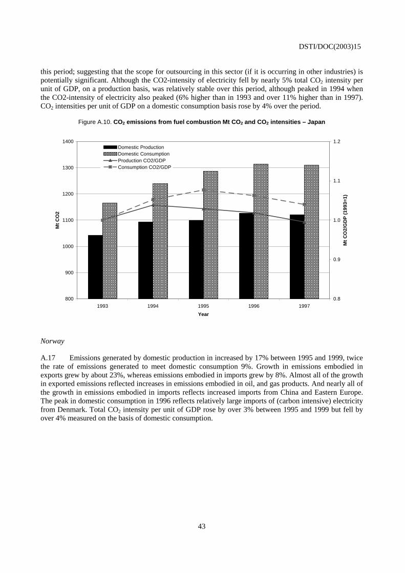
DSTI/DOC(2003)15
43
this period; suggesting that the scope for outsourcing in this sector (if it is occurring in other industries) is potentially significant. Although the CO2-intensity of electricity fell by nearly 5% total CO2 intensity per unit of GDP, on a production basis, was relatively stable over this period, although peaked in 1994 when the CO2-intensity of electricity also peaked (6% higher than in 1993 and over 11% higher than in 1997). CO2 intensities per unit of GDP on a domestic consumption basis rose by 4% over the period.
Figure A.10. CO2 emissions from fuel combustion Mt CO2 and CO2 intensities – Japan
800
900
1000
1100
1200
1300
1400
1993 1994 1995 1996 1997
Year
Mt
CO
2
0.8
0.9
1.0
1.1
1.2
Mt
CO
2/G
DP
(19
93=1
)
Domestic ProductionDomestic ConsumptionProduction CO2/GDPConsumption CO2/GDP
Norway
A.17 Emissions generated by domestic production in increased by 17% between 1995 and 1999, twice the rate of emissions generated to meet domestic consumption 9%. Growth in emissions embodied in exports grew by about 23%, whereas emissions embodied in imports grew by 8%. Almost all of the growth in exported emissions reflected increases in emissions embodied in oil, and gas products. And nearly all of the growth in emissions embodied in imports reflects increased imports from China and Eastern Europe. The peak in domestic consumption in 1996 reflects relatively large imports of (carbon intensive) electricity from Denmark. Total CO2 intensity per unit of GDP rose by over 3% between 1995 and 1999 but fell by over 4% measured on the basis of domestic consumption.
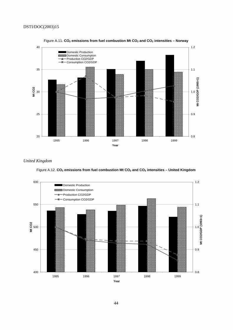
DSTI/DOC(2003)15
44
Figure A.11. CO2 emissions from fuel combustion Mt CO2 and CO2 intensities – Norway
20
25
30
35
40
1995 1996 1997 1998 1999
Year
Mt
CO
2
0.8
0.9
1.0
1.1
1.2
Mt
CO
2/G
DP
(19
95=1
)
Domestic ProductionDomestic ConsumptionProduction CO2/GDPConsumption CO2/GDP
United Kingdom
Figure A.12. CO2 emissions from fuel combustion Mt CO2 and CO2 intensities – United Kingdom
400
450
500
550
600
1995 1996 1997 1998 1999
Year
Mt
CO
2
0.8
0.9
1.0
1.1
1.2
Mt
CO
2/G
DP
(19
93=1
)
Domestic Production
Domestic Consumption
Production CO2/GDP
Consumption CO2/GDP
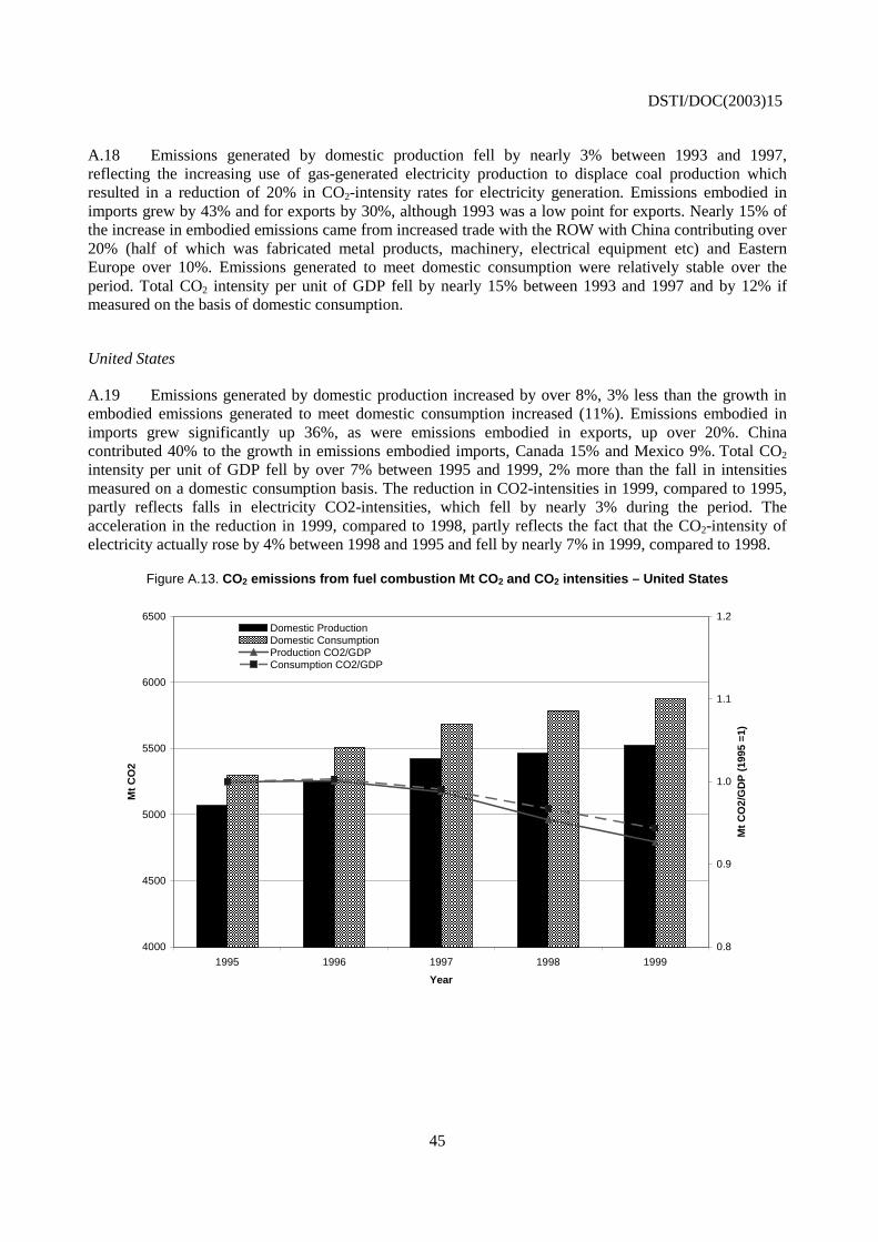
DSTI/DOC(2003)15
45
A.18 Emissions generated by domestic production fell by nearly 3% between 1993 and 1997, reflecting the increasing use of gas-generated electricity production to displace coal production which resulted in a reduction of 20% in CO2-intensity rates for electricity generation. Emissions embodied in imports grew by 43% and for exports by 30%, although 1993 was a low point for exports. Nearly 15% of the increase in embodied emissions came from increased trade with the ROW with China contributing over 20% (half of which was fabricated metal products, machinery, electrical equipment etc) and Eastern Europe over 10%. Emissions generated to meet domestic consumption were relatively stable over the period. Total CO2 intensity per unit of GDP fell by nearly 15% between 1993 and 1997 and by 12% if measured on the basis of domestic consumption.
United States
A.19 Emissions generated by domestic production increased by over 8%, 3% less than the growth in embodied emissions generated to meet domestic consumption increased (11%). Emissions embodied in imports grew significantly up 36%, as were emissions embodied in exports, up over 20%. China contributed 40% to the growth in emissions embodied imports, Canada 15% and Mexico 9%. Total CO2 intensity per unit of GDP fell by over 7% between 1995 and 1999, 2% more than the fall in intensities measured on a domestic consumption basis. The reduction in CO2-intensities in 1999, compared to 1995, partly reflects falls in electricity CO2-intensities, which fell by nearly 3% during the period. The acceleration in the reduction in 1999, compared to 1998, partly reflects the fact that the CO2-intensity of electricity actually rose by 4% between 1998 and 1995 and fell by nearly 7% in 1999, compared to 1998.
Figure A.13. CO2 emissions from fuel combustion Mt CO2 and CO2 intensities – United States
4000
4500
5000
5500
6000
6500
1995 1996 1997 1998 1999
Year
Mt
CO
2
0.8
0.9
1.0
1.1
1.2
Mt
CO
2/G
DP
(19
95 =
1)
Domestic ProductionDomestic ConsumptionProduction CO2/GDPConsumption CO2/GDP
DSTI/DOC(2003)15
46
ANNEX B – DETAILED METHODOLOGY
B.1 The analysis uses three distinct datasets: input-output tables; international trade flows in manufactured products, and estimates of CO2 emissions by industry and country (from the International Energy Agency, IEA).
B.2 The approach is to calculate, for each country:
(1) Domestic CO2 emissions embodied within goods and services and used by domestic consumers (includes, investment, changes in inventories, households and government final consumption) and exports of services;
(2) Domestic CO2 emissions embodied within exports of manufactured products;
(3) Imported CO2 emissions embodied within manufactured products used by final consumers (including emissions from manufactured imports embodied in exports of services);
(4) Imported CO2 emissions embodied within exports of manufactured products.
In this way it is possible to define the domestic consumption of CO2 emissions as the sum of (1) and (3) above, as opposed to domestic production of CO2 emissions, which can be shown to be equal to (2) + (4).
The input-output framework
B.3 Let the production function (input-output table) at a point in time for a country be defined as A, with components, aij that represent the ratio of domestic inputs from industry i to the output of industry j (known as the Leontief matrix) where n is the number of industries, and industries 1 to k (<n) are manufacturing. Further let the import matrix (with dimension k*n) be defined as Mc, with components mcij representing the ratio of manufactured imports from industry i in country c (the exporting country) to the output of domestic industry j at f.o.b. prices. Total CO2 consumed within this economy (assuming no imports of services) can be shown to be equal to:
(I) ( ) DAIE 1−−∗ ( ){ }cm
c
w
cc
m DDAIME +∗−∗∗+ −∑ 1
(1) (3)
Where E is a n∗1 vector of the ratio of CO2 emissions per monetary value of domestic output by industry with zero entries for all service industries; D is an 1∗n vector of domestic consumption28 of domestic
28. “Domestic consumption” includes household final consumption, general government final consumption,
changes in inventories, gross fixed capital formation and valuables, and exports of services but not exports of manufactured products (ISIC 1-40).
DSTI/DOC(2003)15
47
production; cm E is a k∗1 vector of CO2 emissions per unit of country c exports (converted into the
importing country’s currency), and known here as the export emission ratio (emission factor); and cm D is
an 1∗n vector of imports from country c directly purchased as domestic final consumption (not intermediate). W is the total number of exporting countries.
B.4 The first term in equation (I) can be shown to be equivalent to (1) above, (domestic emissions consumed domestically), and the second term can be shown to be equivalent to (3) above, (imported embodied emissions in manufactured products consumed domestically).
B.5 One important point to note is that cm E includes both domestically produced and imported
emissions. The ‘j’th component of which can be shown to be equal to:
(II)
+= ∑w
ddjj
mjjjcj
m ExpExpZE /
(III) ( ) ( ){ }
+∗−∗∗+−∗= −− ∑ dm
dd
w
d
m ExpExpAIMEExpAIEZ 11
(2) (4)
Where Exp is a kn ∗ matrix with components ijExp , where iiExp = exports by domestic industry i in
country c, and all other entries are zero, and dm Exp is an kk ∗ matrix, where diiExp exports of imports
from country d by country c of product i and all other entries are zero; (For most countries all entries of
dm Exp are zero).
B.6 The first term in equation (III) can be shown to be equivalent to (2) above, (domestic emissions embodied within manufactured exports) and the second term to be equivalent to (4), (imported emissions embodied within manufactured exports). It should be evident from equations (II) and (III) that the export
emission ratio cm E involves an iterative process, since it is a function of the export emission ratios in other
countries, which are in turn dependent on cm E . In this study this iterative process was started by setting (4)
above in equation (III) to zero.29
Data
Input-output tables
B.7 Input-Output tables for 24 countries are used in this analysis: Australia 1994/95; Brazil 1996, Canada 1997; China 1997, Czech Republic 1995; Denmark 1997; France 1995; Finland 1995; Germany 1995; Greece 1994; Hungary 1998; India 1993, Italy 1992; Japan 1995 and 1997; Korea 1995; the Netherlands 1995 and 1997; New Zealand 1995/96, Norway 1997; Poland 1995; Russia 1998, Spain 1995; 29. The same results could be achieved by defining an input-output table with dimension ( )wn ∗ by ( )wn ∗ ,
where w is the number of separate countries (or regions) defined in the system, and where sales of services across countries (imports of services) are set to zero.
DSTI/DOC(2003)15
48
Sweden 1998; the United Kingdom 1995; and the United States 1997. All tables are produced on an ISIC Revision 3 basis.
B.8 Most of these tables have been produced by the OECD Secretariat, largely by converting existing country supply and use tables, and are under continued development. This transformation process uses varying degrees of assumption depending on the country, and the aim is to reduce the scale of these assumptions, as more data becomes available.30
B.9 The OECD input-output tables are produced on a 41 industry-by-industry basis but for the purposes of this analysis they have been collapsed to a 17-industry basis, described in Table B.1 below. The sensitivity of the results to the level of aggregation has not been fully tested, although variants produced by allocating IEA emissions data to the 41 industries using fuel combustion have been tested and these did not significantly change the results; largely reflecting the fact that in the 17 industry and 41 industry classifications, those industries where significant direct emissions occur, such as electricity, metals and chemicals, were the same.
Table B.1. Industry classification
Industry ISIC Revision 3 Industries
AGRICULTURE, HUNTING, FORESTRY AND FISHING 01-05 MINING AND QUARRYING & PETROLEUM REFINING 10-14, 23 FOOD PRODUCTS, BEVERAGES & TOBACCO 15-16 TEXTILES, APPAREL & LEATHER 17-19 WOOD & WOOD PRODUCTS 20 PULP, PAPER, PRINTING & PUBLISHING 21-22 CHEMICALS 24 OTHER NON-METALLIC MINERAL PRODUCTS 26 IRON & STEEL 271 2731 NON-FERROUS METALS 272 2732 FABRICATED METAL PRODUCTS, MACHINERY & EQPT 28-32 MOTOR VEHICLES, TRAINS, SHIPS PLANES 34, 35 PLASTICS, OTHER MANUFACTURING & RECYCLING 25, 33, 36-37 ELECTRICITY, GAS 40 CONSTRUCTION 45 TRANSPORT AND STORAGE 60-62 ALL OTHER SERVICES 41, 50-99, ex 60-62
IEA CO2 emissions
B.10 This classification of industries is based on the industry classification used in the International Energy Agency’s database, where CO2
31 emissions by each industry group shown above are readily available. The estimates of CO2 emissions from fuel combustion are calculated using the IEA energy balances together with default methods and emission factors from Revised IPCC Guidelines for National
30. The OECD Input-Output Database, paper presented to 14th International Conference on IO Techniques –
Montreal, October 2002.
31. Further information can be found at www.IEA.org. See also IEA’s annual publication, CO2 Emissions from Fuel Combustion.
DSTI/DOC(2003)15
49
Greenhouse Gas Inventories, using the IPCC Tier 1 Sectoral Approach. For the purposes of this analysis a number of caveats should be added:
• IEA estimates of CO2 emissions from fuel combustion and countries own estimates may differ, although in general these are not significant. This mainly reflects the fact that countries may have more detailed information on emissions from fuel combustion than is available at the IEA. For example the IEA uses an average net calorific value (NCV) for coal, whereas countries may have specific NCVs for production, imports, exports, etc. Equally IEA estimates include emissions from coke inputs into blast furnaces,32 whereas countries may have included these emissions in the IPCC Industrial Process category, and not the Fuel combustion category used here. IEA fuel data comes directly from IEA member Countries.
• One industrial sector of IEA data warrants specific mention since emissions in this sector have not been included in the main results presented in Section 3: Unallocated Auto-producers. This sector includes emissions from producers that generate their own electricity or heat, wholly or partly, for their own use as an activity that supports their primary activity. Ideally these emissions should be allocated to the actual ISIC industry where the producers are classified but it has not been possible to do that here, and so all of these emissions are included within the domestic consumption and domestic production figures for each country, but not estimates of emissions embodied in imports or exports. That said these emissions are not particularly significant in the context of the estimates presented above for most countries, for example, in the United States, emissions from Unallocated Auto-producers made up about 5% of total emissions in 1997. As manufactured exports make up about 6% of total final demand (of domestic products) in the United States, most of the emissions from auto producers can be expected to be embodied within products consumed domestically. Although much depends on which industries are actually responsible for the emissions. For example the chemicals industry exported a relatively high 16% of its output in 1997. If all Auto-producer emissions came from this industry, emissions embodied in exports would be higher by at least 1% of total US emissions (equivalent to a 20% increase on the export figures shown in Table 3). However, including emissions by Auto-producers in other countries would increase emissions embodied in US imports, meaning that the overall trade balance would be less affected. For some countries however the size of Auto-producers is significant, in particular Russia (and, less so, Korea, see Table 2), and so estimates of emissions embodied in Russian exports are particularly affected (biased downwards), (see also below).
• Emissions from transport use have not been included in the main results presented in Section 3 because the IEA data do not specify which industries have been responsible for the emissions since the emissions data are calculated on the basis of the carbon content of petrel/diesel designated for transport use, supplied into an economy, not by user. Indeed the total figure for emissions related to transportation includes households and not just industries. It is possible to estimate the emissions in each sector by applying carbon coefficients to their purchases of petrol. However this may introduce systematic biases in the results based on the geographical size of countries. The bias comes about because estimates of the value of transportation within imports (which are measured on c.i.f.33 basis) are not available. If, for
32. In the reduction of iron in a blast furnace through the combustion of coke, the primary purpose of coke
oxidation is to produce pig iron and the emissions can be considered as in industrial process, as is the practice in some countries, these emissions are included in fuel combustion emissions in the IEA statistics.
33. C.I.F (cost, insurance, freight) prices show the value of imports at the importing country’s frontier, including the insurance and freight charges incurred between the exporter’s frontier and that of the importer.
DSTI/DOC(2003)15
50
any product, emissions from fuel-used in domestic transportation were embodied but estimates from foreign transportation were not an inconsistency and potential bias would be introduced. For example it would mean that fuel used in transporting a good from the East-Coast to the West-Coast of the United States would be embodied within the good but fuel used in transporting the same good from Spain, say, to the West-Coast would not, and so emissions embodied in US produced goods would appear to be higher, even if the production process in the United States was the same as that in Spain. It is possible however to provide illustrative estimates of these embodied emissions, using stylised assumptions which attempt to overcome this bias, and these are shown in Figures B4 and B5.
• IEA emissions data covers only CO2 emissions from fuel combustion. (Fossil fuel production and use are responsible for about three-quarters of anthropogenic CO2 emissions). Other GHGs might be important for some industries (e.g. aluminium emits PFCs) but these are not taken into account in this study.
Bilateral trade
B.11 The OECD Bilateral Trade Database34 shows imports into and exports from 41 countries/regions,35 by producing country and destination country, for all two-digit products within ISIC 01-40. The countries/regions covered are: all OECD countries, Argentina, Brazil, China, Hong Kong (China), India, Indonesia, Malaysia, the Philippines, Singapore, Thailand, Taiwan, and the Rest of the World (ROW).
B.12 There are some data quality issues concerning the bilateral trade database. The first relates to the fact that imports by country A from country B are not always consistent with exports from country B to country A. This is partly because exports are on an f.o.b.36 basis whereas imports are recorded c.i.f. (this study assumes that 10% of the import value reflects transportation and insurance costs) but other factors play a part too. For example a lot of trade from China goes through Hong-Kong, and Chinese data may record this trade as exports to Hong-Kong, whereas reporting-importing countries may record the goods as having come from China, not Hong-Kong. Equally the bilateral trade data are not always consistent with the equivalent country totals shown in the corresponding input-output tables.
B.13 Ideally CO2 emissions embodied in imports of services would also be recorded in the estimates shown in Section 3. The lack of bilateral trade data in services makes it difficult to do this, and so, in Section 3, emissions associated with trade in services (e.g. air travel) are included within both domestic consumption and production estimates but not emissions embodied in imports or exports. The input-output tables do however contain estimates of trade in services, and so provide a possible starting point for estimating embodied emissions in international trade in services, assuming an internationally common emissions factor for services. However in adopting this approach it is important to have estimates of imports by product on an f.o.b. basis; which is rarely the case. Not accommodating for c.i.f./f.o.b. differences is a common error in much of the literature on this subject and is likely to contribute to the general pattern of low total CO2 emissions embodied in imports, relative to total CO2 embodied in exports, often recorded in these analyses, since exports of transport services usually have relatively high emissions
34. Source: OECD Bilateral Trade Database, Science Technology and Industry Directorate.
35. Bilateral trade between non-member countries is not covered however, for example Brazil’s exports to Argentina are not shown in the database.
36. F.O.B (free-on-board) prices are valued at the exporter’s frontier value.
DSTI/DOC(2003)15
51
factors. In the analysis shown in Section 3 direct emissions from the service sector (including transportation emissions) are not included in estimates of emissions embodied in international trade. Estimates are however produced for illustration in Figures B4 and B5 below, using the approach outlined above estimating the c.i.f/f.o.b difference for each product, and described in more detail in Paragraph B42.
Assumptions
B.14 The section that follows focuses primarily on the assumptions used to develop the data sources needed in this analysis. It does not focus on the conventional input-output assumptions; which are described in general terms in Section 2. One IO assumption that is worth mentioning here however concerns differential pricing, namely that the analysis assumes that goods produced in any country are sold for the same price in the domestic market as abroad and that domestic consumers, whether industries or households, pay the same price for all goods produced domestically. In some key industries, such as electricity, this is rarely the case. Households tend to pay more per KWh of electricity than industries, and this means that emission factors for manufactured goods are likely to be lower than they would be if it were possible to correct for differential pricing in electricity.
Estimating emission factors in countries where IO data are not available
B.15 For those countries/regions where input-output tables are not available, export emissions’ ratios have been estimated on the basis of the emissions ratios of countries that are believed to have similar emissions profiles and production processes, except for electricity generation and oil and gas extraction in OPEC countries.
Austria – (emission factors proxied by Germany); Belgium – (the Netherlands); Iceland – (Denmark); Ireland – (United Kingdom); Mexico – (United States); Portugal – (Spain); Slovakia – (Czech Republic); Switzerland – (Germany); Turkey – (Greece); Argentina – (Brazil); Hong-Kong, Indonesia, Malaysia, Philippines, Singapore, Taiwan, OPEC countries (excluding oil) – (Korea); Rest of the World – (United States).
Adjusting for differences in electricity generation
B.16 Emission factors in each country are adjusted to reflect known differences in the carbon-intensity of electricity generation. The way in which this adjustment is implemented is best described by an example. Electricity produced in Germany for example produces nearly three times as much CO2 emissions per KWh of electricity than in Austria. To estimate Austrian emission factors we assume that the production process of each industry in Austria is the same as that in Germany, except that electricity is three times less carbon intensive. So, for given unit of Austrian manufactured output, embodied emissions that reflect electricity inputs are three times lower than in Germany. In other words, in equation (I) above, the component for Austrian electricity in vector “E” is one-third that of Germany’s. All other components of the equation remain the same as their German equivalents.
Gas and oil – extraction & refining
B.17 Emission factors for oil and gas extraction for OPEC countries have been separately estimated by taking IEA estimates of direct emissions by the “crude/refined oil and gas” sector in each OPEC country and dividing these figures by the USD value of crude/refined oil and gas output in each country. An
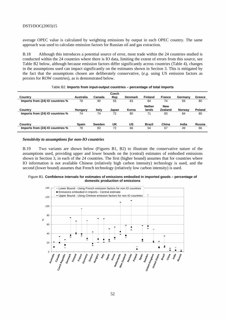
DSTI/DOC(2003)15
52
average OPEC value is calculated by weighting emissions by output in each OPEC country. The same approach was used to calculate emission factors for Russian oil and gas extraction.
B.18 Although this introduces a potential source of error, most trade within the 24 countries studied is conducted within the 24 countries where there is IO data, limiting the extent of errors from this source, see Table B2 below, although because emission factors differ significantly across countries (Table 4), changes in the assumptions used can impact significantly on the estimates shown in Section 3. This is mitigated by the fact that the assumptions chosen are deliberately conservative, (e.g. using US emission factors as proxies for ROW countries), as is demonstrated below.
Table B2. Imports from input-output countries – percentage of total imports
Country Australia Canada Czech Rep Denmark Finland France Germany Greece
Imports from (24) IO countries % 78 90 55 83 84 74 69 80
Country Hungary Italy Japan Korea Nether lands
New Zealand Norway Poland
Imports from (24) IO countries % 74 74 72 80 71 83 84 80
Country Spain Sweden UK US Brazil China India Russia Imports from (24) IO countries % 78 83 72 66 54 67 49 66
Sensitivity to assumptions for non-IO countries
B.19 Two variants are shown below (Figures B1, B2) to illustrate the conservative nature of the assumptions used, providing upper and lower bounds on the (central) estimates of embodied emissions shown in Section 3, in each of the 24 countries. The first (higher bound) assumes that for countries where IO information is not available Chinese (relatively high carbon intensity) technology is used, and the second (lower bound) assumes that French technology (relatively low carbon intensity) is used.
Figure B1. Confidence intervals for estimates of emissions embodied in imported goods – percentage of domestic production of emissions
0
20
40
60
80
100
120
140
Aus
tral
iaC
anad
aC
zech
Rep
ublic
Den
mar
kFi
nlan
dFr
ance
Ger
man
yG
reec
eH
unga
ry
Italy
Japa
nK
orea
Net
herl
ands
New
Zea
land
Nor
way
Pol
and
Spa
inS
wed
enU
nite
d K
ingd
omU
nite
d S
tate
s
Bra
zil
Chi
na
Indi
aR
ussi
a
%
Lower Bound - Using French emission factors for non IO countriesEmissions embodied in imports - Central estimateUpper Bound - Using Chinese emission factors for non IO countries
DSTI/DOC(2003)15
53
Figure B2. Confidence intervals for estimates of emissions embodied in exported goods – percentage of domestic production of emissions
0
20
40
60
80
100
120A
ustr
alia
Can
ada
Cze
ch R
epub
licD
enm
ark
Finl
and
Fran
ceG
erm
any
Gre
ece
Hun
gary
Italy
Japa
nK
orea
Net
herl
ands
New
Zea
land
Nor
way
Pol
and
Spa
inS
wed
enU
nite
d K
ingd
omU
nite
d S
tate
s
Bra
zil
Chi
na
Indi
aR
ussi
a
%
Lower Bound - Using French emission factors for non IO countriesEmissions embodied in exports - Central estimateUpper Bound - Using Chinese emission factors for non IO countries
B.20 In both charts the central estimates are much closer close to the lower bound, confirming the conservative nature of the estimates used in the main analysis but at the same time illustrating the potentially (significantly) larger size of embodied emissions if less conservative assumptions concerning technology used in other countries are adopted. Figure B2 also illustrates the double-accounting nature of embodied emissions reflecting that fact that imports can also be embodied in exports, whether directly, as re-exports in some countries, or indirectly as intermediate consumption of goods destined for export. Those countries with large upper limits tend to be those with relatively high exposure to trade, particularly those with significant direct re-exports of imports, and where IO tables with important trading partners are not available, e.g. the Netherlands, which has significant trade with Belgium, relatively high exposure to international trade, and relatively high levels of re-exports as a percentage of total exports.
B.21 As the coverage of the OECD IO database expands so to will the ratios in Table B2 rise. In this context the inclusion of IO tables for high trade, high emission non-member OECD countries, such as Singapore, Malaysia, Indonesia, and Chinese Taipei is as important as the inclusion of other OECD member countries, such as Mexico, although the importance of each country varies according to the importing country, Mexico for example is very important for the US statistics as are Asian economies to Japan.
Coherence between IEA emissions data and input-output tables
B.22 The analysis assumes coherence in industrial classifications. Both the IEA data and input-output data are based on ISIC rev 3 classifications but it is difficult to ensure, without further investigation, that establishments in both data sets have been allocated consistently.
Bilateral trade data – allocation of imports to industries
B.23 Bilateral trade data cannot identify which domestic industries are responsible for imports. This has been estimated using import proportions in the input-output framework for each country. So for
DSTI/DOC(2003)15
54
example, for country A, if industry A1 imports 10% of total economy imports of product Y, (40% of which comes from country B and 60% from country C), the model assumes that 4% of Y from country B and 6% of Y from country C are imported by industry A1.
Differences in IO years
B.24 Because not all input-output tables cover the same year, emissions embodied in exports from country A to country B in year t, have been converted to emissions embodied in imports into country B from country A by assuming that the emission ratio is constant for given volume of output for each product. For ISIC industries 1-27, US output deflators at the ISIC two-digit level are applied to bilateral trade data in dollar prices. For manufactured goods however ISIC 28-37 (which includes electronic goods, etc) quality changes have occurred, and deflators based on the prices of these goods will overestimate volume movements in imports and exports (if quality improves). To proxy volume change, deflators are constructed, for each product, by weighting the price increases in ISIC 1-27 goods by the intermediate consumption of these goods, for each two-digit industry in ISIC 28-37, in each country. Nevertheless, the results shown in Section 3 are relatively insensitive to the use of these adjusted deflators compared to conventional deflators based on (quality-adjusted) movements in prices, since most IO tables cover the period 95-97 (the smaller the period of time the less likely the change in deflators), and because, for most countries, most trade occurs with countries that have IO tables in the same year. For example the US tables are for 1997, and IO tables with its key trading partners are also available in this year: Canada, China, Japan, as well as Denmark, the Netherlands, Norway.
Interpreting emission factors – Table 4
B.25 Some emission factors in Table 4 are difficult to explain, for example the relatively high emission factors for mining, extraction and refining in the United States and Canada; much of which reflects “flaring”. Why both countries should have double the ratios of the United Kingdom, say, is odd. It may be that US/Canadian rigs re-inject proportionally less excess gas into reservoirs than they burn but it has not been possible to establish this for the purposes of this paper, and will be the subject of further inquiries.
B.26 The emission factors are presented as Mt CO2 per billion USD and this conversion to USD has the potential to introduce biases in emission factors. For example Italian emission factors in 1995 are based on Italian input-output tables in 1992, converted to USD and projected forward into 1995 prices, using US output deflators. The projection to 1995 prices is a possible source of bias/error in this formulation but in this context the Lira/USD exchange rate and the use of US deflators is critical. Unusual currency strength will lead to relatively low emission factors and vice versa. In 1992, on average, ITL 1 232 bought one US dollar, rising to ITL 1 574 in 1993 and 1 629 Lira in 1995 (depreciation in the Lira relative to the US dollar), meaning that the emission factors for Italy in 1995 may be biased downwards.
B.27 Volatility in exchange rates is also important, since average annual exchange rates are used for conversion and these may not reflect the average rate actually paid by one country for the exports of another in the same year. This is of particular importance for Russian emission factors; since the rouble/USD exchange rate was extremely volatile in 1998 (the Russian IO year). At the beginning of 1998 the rate was six roubles to the US dollar but by the end the year the rate was 21.5. (For prudence the results shown above assume an average rate of eight; higher rates would lead to higher Russian emission factors.)
B.28 Additionally, the emission factors assume that the prices of exported goods and the same goods on the domestic market are the same and that each industry exports the same basket of goods as the goods produced and sold on the domestic market; and these conditions may not always hold. Although the impact of these assumptions is not expected to have a significant impact on total emissions embodied in imports, the same cannot necessarily be said for emission embodied in exports.
DSTI/DOC(2003)15
55
B.29 Moreover, a high emissions factor for a product in one country compared to the same product in another may reflect differences in purchasing power or prices, and not differences in energy efficiency. For example although Russian iron and steel emission factors (measured in emissions per US dollar) are roughly six times as high as emission factors in other countries about half of this reflects the fact that Russian steel costs significantly less than steel produced in developing economies (partly reflecting differences in quality and product mix but exacerbated by the collapse of the Rouble in 1998). For example between the beginning of 1998 and the end of 199937 the price of steel sections produced in Russia (CIS)collapsed from a high of USD 330 per tonne to USD 175 per tonne, whereas European Coal and Steel Community (ECSC) prices fell from USD 430 to USD 310 per tonne.
B.30 Product differences also play a significant role, reflecting the heterogeneity of the iron and steel classification. For example the price of stainless steel produced in the European Coal and Steel Community in 1998 ranged from USD 1 150 to USD 1 650 per tonne, whereas Russian (CIS) of pig-iron cost little over USD 100 per tonne. In producing stainless steel most emissions embodied in the steel reflect emissions embodied in pig-iron used to produce the steel, in other words the emission factors per tonne of stainless steel and pig-iron are not likely to be significantly different. But in cash terms pig-iron can have emission factors over ten times as high.
B.31 This provides a possible explanation for the high iron and steel emission factors shown in Table 3 for India, China and Russia compared to developing economies. Indeed assuming steel prices (reflecting quality and product mix) differed by a factor of two, emissions factors (if measured per tonne of iron or steel, rather than USD) in these countries would be only about three times those of developed economies, rather than six times. In Eastern Europe, prices of steel products were about 20-25% lower than those of developed economies during the late 1990s, bringing the emission factors (per tonne) in this group of countries down to about twice those of developed economies.
B.32 Put in the context of product and energy-intensity differences, the range of emission factors for iron and steel (adjusted for price differences) is explainable. For example steel produced in open-hearth furnaces requires over five times more energy than basic oxygen furnaces. Although the former are gradually being phased out they still represented 5% and 14% of production in China and India in 1998 (source: International Iron and Steel Institute). Of course, steel can also be produced using scrap metal, rather than iron-ore/pig-iron, and this is much less energy-intensive, since scrap is considered to have zero embodied emissions in the accounting framework we use. To underpin the importance of steel to embodied emissions in trade between developing and developed economies China became the world’s largest producer of steel in 1996 (IISI, 1999).
B.33 For illustration Table B3 shows emission factors adjusted for total economy (GDP) differences in purchasing power parities (PPP). Although not perfect, since GDP based PPPs reflect services as well as goods (and differences in relative prices for services are likely to higher than goods), Table B3 helps to illustrate that simple comparisons of the carbon-intensities shown in Table 4a can be misleading when taken as proxies for carbon-intensities based on quantity measures. It suggests that the range of carbon-intensities, adjusted for differences in relative prices, is likely to be smaller. For example a comparison of carbon-intensities in Table 4a, shows that, per unit USD, Russian steel is six times more carbon-intensive than US steel. Adjusting for differences in PPPs however brings this ratio down to two, which is much closer to the difference in carbon-intensities in steel production per tonne suggested above.
37. Source: Metal Bulletin. Russian data for steel sections is not available for end-1998 but the price of steel
produced elsewhere suggests most of the price-fall between start-98 and end-99 occurred by end-1998.
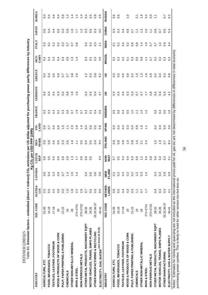
DST
I/D
OC
(200
3)15
56
Tab
le B
3. E
mis
sio
n f
acto
rs –
em
bo
die
d (
dir
ect
+ in
dir
ect)
CO
2 em
issi
on
s p
er U
S d
olla
r ad
just
ed f
or
pu
rch
asin
g p
ow
er p
arit
y d
iffe
ren
ces
by
ind
ust
ry
K
g C
O2
per
US
D P
PP
(19
95)
IND
UST
RY
IS
IC C
OD
E
AU
STR
A-
LIA
C
AN
AD
A
CZ
EC
H
RE
P
DE
N-
MA
RK
F
IN-
LA
ND
F
RA
NC
E
GE
RM
AN
Y
GR
EE
CE
H
UN
-G
AR
Y
ITA
LY
JA
PA
N
KO
RE
A
AG
RIC
UL
TU
RE
, ET
C
01-0
5 0.
5 0.
6 0.
6 0.
8 0.
6 0.
3 0.
4 0.
4 0.
4 0.
3 0.
6 0.
4
FO
OD
, BE
VE
RA
GE
S, T
OB
AC
CO
15
-16
0.5
0.4
0.5
0.8
0.7
0.3
0.4
0.4
0.4
0.2
0.4
0.4
TE
XT
ILE
S, L
EA
TH
ER
, FO
OTW
EA
R
17-1
9 0.
5 0.
3 0.
5 0.
6 0.
5 0.
3 0.
5 0.
5 0.
3 0.
2 0.
4 0.
6
WO
OD
& P
RO
DU
CT
S O
F W
OO
D &
CO
RK
20
0.
5 0.
4 0.
5 0.
5 0.
6 0.
2 0.
3 0.
6 0.
4 0.
2 0.
5 0.
4
PU
LP
, PA
PE
R P
RIN
TIN
G &
PU
BL
ISH
ING
21
-22
0.5
0.7
0.6
0.3
1.0
0.3
0.4
0.7
0.4
0.3
0.4
0.6
CH
EM
ICA
LS
24
1.
0 1.
4 0.
9 0.
6 1.
1 0.
6 0.
8 0.
7 0.
9 0.
7 0.
9 1.
2
OT
HE
R N
ON
-ME
TA
LL
IC M
INE
RA
L
26
1.6
1.0
1.3
1.6
2.3
0.7
1.0
3.8
1.3
0.7
1.0
1.4
IRO
N &
ST
EE
L
271+
2731
2.
2 1.
4 1.
7 1.
1 2.
8 1.
9 1.
6 2.
6 1.
4 0.
8 1.
7 1.
2
NO
N-F
ER
RO
US
ME
TA
LS
27
2+27
32
2.9
0.
8 0.
5 1.
4 0.
7
1.
2 1.
4
OT
HE
R M
ET
AL
PR
OD
UC
TS
, MA
CH
INE
RY
EQ
PT
28
-32
0.7
0.4
0.6
0.4
0.4
0.2
0.4
1.2
0.3
0.2
0.3
0.4
MO
TO
R V
EH
ICL
ES
, TR
AIN
S, S
HIP
S P
LA
NE
S
34,3
5 0.
5 0.
6 0.
5 0.
5 0.
6 0.
2 0.
4 0.
3 0.
2 0.
2 0.
5 0.
5
OT
HE
R M
AN
UF
AC
TU
RIN
G &
RE
CY
CL
ING
25
,33,
36-3
7 0.
5 0.
6
0.4
0.5
0.4
0.4
0.8
0.3
0.3
0.3
0.8
EL
EC
TR
ICIT
Y, G
AS
, WA
TE
R (s
ee A
nn
ex B
, B.3
3)
40-4
1 8.
6 3.
8 4.
4 9.
4 5.
8 0.
6 4.
7 6.
2 4.
0 2.
1 3.
0 4.
6
IND
US
TR
Y
ISIC
CO
DE
N
ET
HE
R-
LA
ND
S
NE
W
Z’L
AN
D
NO
R-
WA
Y
PO
LA
ND
S
PA
IN
SW
ED
EN
U
K
US
B
RA
ZIL
IN
DIA
C
HIN
A
RU
SS
IA
AG
RIC
UL
TU
RE
, ET
C
01-0
5 0.
8 0.
2 0.
7 0.
9 0.
3 0.
5 0.
3 0.
5 0.
2 0.
1 0.
3 0.
6
FO
OD
, BE
VE
RA
GE
S, T
OB
AC
CO
15
-16
0.5
0.2
0.5
0.8
0.4
0.6
0.4
0.5
0.2
0.2
0.4
0.6
TE
XT
ILE
S, L
EA
TH
ER
, FO
OTW
EA
R
17-1
9 0.
4 0.
3 0.
3 0.
8 0.
4 0.
4 0.
4 0.
5 0.
2 0.
5 0.
4
WO
OD
& P
RO
DU
CT
S O
F W
OO
D &
CO
RK
20
0.
3 0.
2 0.
4 1.
0 0.
3 0.
5 0.
3 0.
6 0.
1 0.
2 0.
6 1.
0
PU
LP
, PA
PE
R P
RIN
TIN
G &
PU
BL
ISH
ING
21
-22
0.3
0.2
0.3
0.8
0.4
1.0
0.3
0.4
0.3
0.6
0.7
CH
EM
ICA
LS
24
1.
1 1.
2 0.
9 1.
5 0.
8 1.
1 0.
7 1.
0 0.
5 0.
8 1.
1 2.
1
OT
HE
R N
ON
-ME
TA
LL
IC M
INE
RA
L
26
0.7
0.3
1.2
2.1
1.0
1.0
0.7
1.3
0.6
1.4
1.3
1.9
IRO
N &
ST
EE
L
271+
2731
1.
7 1.
4 3.
3 2.
4 1.
1 1.
2 1.
7 1.
6 1.
1 1.
9 2.
0 3.
2
NO
N-F
ER
RO
US
ME
TA
LS
27
2+27
32
0.8
0.
8 0.
9 0.
7 0.
7 1.
1 0.
9
OT
HE
R M
ET
AL
PR
OD
UC
TS
, MA
CH
INE
RY
EQ
PT
28
-32
0.4
0.3
0.4
1.0
0.4
0.6
0.4
0.4
0.2
0.7
0.6
1.1
MO
TO
R V
EH
ICL
ES
, TR
AIN
S, S
HIP
S P
LA
NE
S
34,3
5 0.
3 0.
3 0.
4 1.
0 0.
4 0.
4 0.
4 0.
4 0.
2 1.
0 0.
7
OT
HE
R M
AN
UF
AC
TU
RIN
G
25,3
3,36
-37
0.3
0.9
0.3
0.7
0.4
0.6
0.4
0.3
0.2
0.9
0.5
0.7
EL
EC
TR
ICIT
Y, G
AS
& W
AT
ER
SU
PP
LY
40
-41
4.1
0.9
0.1
8.4
3.0
1.8
4.2
6.8
0.3
4.4
5.3
6.2
Not
es:
Est
imat
es fo
r m
inin
g an
d qu
arry
ing
are
not i
nclu
ded
as th
e in
tern
atio
nal p
rices
pai
d fo
r oi
l, ga
s et
c ar
e no
t det
erm
ined
by
diffe
renc
es in
diff
eren
ces
in to
tal e
cono
my
purc
hasi
ng p
ower
par
ities
. Thi
s is
like
ly to
hol
d fo
r ot
her
sect
ors
too
but l
ess
so.
DSTI/DOC(2003)15
57
Electricity
B.34 The problem of international price differences for the same good is particularly noticeable in the emissions factors for electricity. However electricity differs from other products in so far as it is not particularly exposed to international trade; on account of the fact that it is in general not traded. Certainly, for most countries, imports and exports of electricity are zero or insignificant. Nonetheless emission factors have been included in Table 3 for each country, even if electricity is not traded, to reflect the fact that countries with high emission factors for electricity usually also have relatively high emission factors in other industries. This is no coincidence. Electricity makes up a significant part of embodied emissions in nearly every country (except those that use renewable energy sources). The cheaper the electricity the less the incentive for industries to use less electricity in their production processes. In this way it is clear that a higher emission factor for electricity in one country compared to another does not necessarily mean that the electricity generating process is itself more energy-intensive. Table B4 below illustrates this point, by showing CO2 emissions per terawatt hour (TWH) of electricity generated in each of the 24 countries used in this study.
Table B3. Electricity emissions (direct)
Country Australia Canada Czech Rep Denmark Finland France Germany Greece
Mt CO2 emissions per TWH 0.75 0.17 0.48 0.42 0.22 0.04 0.43 0.86
Electricity industry direct emissions % of total domestic emissions 46 21 42 54 36 5 32 50
Country Hungary Italy Japan Korea Nether lands
New Zealand Norway Poland
CO2 emissions per TWH 0.39 0.45 0.32 0.39 0.46 0.08 0.00 0.61
Electricity industry direct emissions % of total domestic emissions 41 26 29 21 26 11 1 48 Country Spain Sweden UK US Brazil China India Russia
CO2 emissions per TWH 0.41 0.04 0.50 0.52 0.03 0.75 0.90 0.18 Electricity industry direct emissions % of total domestic emissions 29 15 33 37 4 39 40 34
B.35 Table B3 shows that although Russia has high emission factors for electricity (Table 4), this is entirely a price effect and not an indication that Russian electricity is more carbon intensive than in most other countries. In fact it shows that Russian electricity is relatively carbon-free compared to other countries.
B.36 It’s important to stress however that the comments made in the preceding paragraphs relate only to the issue of interpreting emission factors, and not the estimates of CO2 embodied in trade, since the estimates of embodied emissions are not, all other things equal, affected by relative differences in the prices of (ostensibly the same) products in any particular country.
B.37 The importance of electricity to embodied emissions and emission factors can be determined by showing the contribution of electricity to emission factors for each product in each country. Table B4, illustrates this breaking down embodied emissions from electricity into two sources, emissions embodied from domestically produced electricity (columns D, below), and emissions embodied from electricity generation abroad (columns I below). For example, in Australia, 43% of all emissions embodied in pulp, paper, printing and publishing products originated in the domestic electricity generation industry, and 8% originated from electricity generation abroad.
DSTI/DOC(2003)15
58
B.38 In all countries the contribution of electricity is significant, particular in countries with carbon-intensive electricity generation, such as Greece. The percentages in Russia are surprisingly high however given the fact that Russia electricity is not relatively carbon-intensive; suggesting that electricity needs in Russian manufacturing are generally considerably higher than in other countries (for example, domestically generated electricity makes up over 60% of emissions embodied in manufactured products in ISIC 28-37, higher than China and India who have more carbon intensive electricity generation), or that electricity is used inefficiently, perhaps reflecting relatively cheap prices.
B.39 Sweden also has relatively high contributions from electricity, but given its relatively low emission factors, this could reflect the fact that production processes, excluding electricity, are also generally low compared to other countries, and not necessarily the fact that electricity use is higher in Swedish industries than equivalent industries abroad.
B.40 Table B4 can be used to indicate the sensitivity of industries in different countries to price rises in domestic electricity generation (although it would be better to look at the contribution of electricity in monetary values, which is not shown but can be derived using IO tables).
B.41 In this context it is important to recall that even in those industries with low direct emissions, such as motor vehicles say, increased production and competition from non-Annex I countries can potentially lead to significant increases in global emissions, since the indirect emissions generated to produce motor vehicles in Annex I countries are significantly higher than Annex I countries (Table 3). Policies that increase the price of electricity in Annex I countries therefore, might reduce the competitiveness of Annex I countries in these (generally low emission) industries, resulting in increased production in non-Annex I countries. However international electricity prices already differ significantly, so electricity price increases might not necessarily reduce competitiveness (Figure B3), although evidence suggests that, in some countries at least, relatively high electricity prices have led to a diversification away from industries with high direct electricity requirements see Paragraph 3.26.
D
STI/
DO
C(2
003)
15
59
Tab
le B
5. C
on
trib
uti
on
of
emb
od
ied
, do
mes
tica
lly p
rod
uce
d a
nd
imp
ort
ed, e
lect
rici
ty t
o e
mis
sio
n f
acto
rs –
%
IND
UST
RY
ISIC
CO
DE
AUST
RAL
IA
CAN
ADA
CZE
CH
R
EP
DEN
MAR
K FI
NLA
ND
FR
ANC
E G
ERM
ANY
GR
EEC
E H
UN
GAR
Y IT
ALY
JAPA
N
KOR
EA
From
dom
esttic
/fore
ign g
ener
ation
(D) /
(I).
D
I
D
I D
I
D
I D
I
D
I D
I
D
I D
I
D
I D
I
D
I
AGR
ICU
LTU
RE,
ETC
01
-05
37
6 15
6
32
4 26
6
20
11
3 13
31
8
32
5 28
9
17
6 7
6 10
9
MIN
ING
, EXT
RAC
TIO
N, R
EFIN
ING
10
-14,
23
24
4 8
2 39
15
5
7 9
24
1 24
12
16
16
30
17
20
5
26
4 32
9
41
FOO
D, B
EVER
AGES
, TO
BAC
CO
15
-16
46
4 24
10
42
5
32
7 25
16
5
15
33
11
40
5 35
12
24
10
21
13
18
12
TE
XTIL
ES, L
EATH
ER, F
OO
TWEA
R
17-1
9 38
15
24
24
42
6
24
26
19
26
4 29
28
21
63
7
37
22
29
16
23
16
19
18
WO
OD
& P
RO
DU
CTS
OF
WO
OD
& C
OR
K 20
51
6
26
7 45
5
31
19
31
13
7 25
39
14
74
6
38
20
27
21
15
15
22
21
PULP
, PAP
ER P
RIN
TIN
G &
PU
BLIS
HIN
G
21-2
2 43
8
27
5 34
7
39
15
42
15
4 19
34
12
61
7
34
21
24
11
27
10
23
13
CH
EMIC
ALS
24
31
7
11
4 36
7
29
14
24
19
3 13
19
9
54
8 25
11
13
9
21
14
13
18
OTH
ER N
ON
-MET
ALLI
C M
INER
AL
26
32
2 16
5
37
4 20
5
8 6
3 7
23
4 31
1
25
7 18
5
14
8 16
6
IRO
N &
STE
EL
271+
2731
18
2
15
7 21
4
37
11
6 11
1
7 15
11
55
5
23
10
17
11
12
8 22
19
N
ON
-FER
RO
US
MET
ALS
272+
2732
30
2
n/a
n/a
27
16
24
32
20
25
3 31
n/
a n/
a n/
a n/
a n/
a n/
a n/
a n/
a 11
33
14
34
O
THER
MET
AL P
RO
DU
CTS
, MAC
HIN
ERY
EQPT
28
-32
40
7 13
16
38
7
26
21
16
25
3 26
30
17
61
8
23
26
20
17
26
16
20
23
MO
TOR
VEH
ICLE
S, T
RAI
NS,
SH
IPS
PLAN
ES
34,3
5 33
9
10
19
38
6 27
19
17
22
3
28
27
18
57
11
18
29
23
16
18
10
18
20
OTH
ER M
ANU
FAC
TUR
ING
& R
ECYC
LIN
G
25,3
3,36
-37
40
10
14
9 n/
a n/
a 33
19
25
26
3
18
31
16
52
5 39
20
25
16
28
17
14
13
IND
UST
RY
ISIC
CO
DE
NET
HER
LAN
DS
NEW
Z’
LAN
D
NO
R W
AY
POLA
ND
SP
AIN
SW
EDEN
U
K U
S BR
AZIL
IN
DIA
C
HIN
A R
USS
IA
D
I D
I
D
I D
I
D
I D
I
D
I D
I
D
I D
I
D
I D
I
AGR
ICU
LTU
RE,
ETC
01
-05
23
4 8
12
0 8
35
2 25
7
12
11
28
9 31
4
2 5
69
2 41
1
48
1 M
ININ
G, E
XTR
ACTI
ON
, REE
FIN
ING
10
-14,
23
2 22
3
3 0
2 36
8
7 26
6
13
8 3
21
7 2
7 32
5
42
1 48
0
FOO
D, B
EVER
AGES
, TO
BAC
CO
15
-16
21
12
12
14
0 14
41
3
27
10
13
15
29
10
35
4 4
6 61
2
39
1 56
1
TEXT
ILES
, LEA
THER
, FO
OTW
EAR
17
-19
17
24
6 29
0
30
52
4 24
16
20
26
24
19
42
8
5 13
63
2
42
3 n/
a n/
a W
OO
D &
PR
OD
UC
TS O
F W
OO
D &
CO
RK
20
24
27
14
16
0 20
54
2
32
18
20
17
34
19
33
4 5
7 21
1
42
1 76
0
PULP
, PAP
ER P
RIN
TIN
G &
PU
BLIS
HIN
G
21-2
2 21
22
19
19
0
15
46
4 27
13
9
9 28
14
37
4
4 6
46
2 46
1
n/a
n/a
CH
EMIC
ALS
24
8
11
3 17
0
12
35
2 16
10
10
10
21
9
26
4 2
8 39
2
43
1 63
1
OTH
ER N
ON
-MET
ALLI
C M
INER
AL
26
15
12
10
15
0 6
23
2 19
3
14
8 25
6
27
3 2
2 25
2
33
1 52
0
IRO
N &
STE
EL
271+
2731
10
8
7 8
0 4
30
3 18
10
9
15
16
5 25
3
1 3
18
1 26
1
25
0 N
ON
-FER
RO
US
MET
ALS
272+
2732
n/
a n/
a n/
a n/
a 0
43
n/a
n/a
n/a
n/a
n/a
n/a
24
23
36
8 3
7 63
3
52
1 62
1
OTH
ER M
ETAL
PR
OD
UC
TS, M
ACH
INER
Y EQ
PT
28-3
2 16
21
6
15
0 27
49
5
24
17
11
25
27
18
40
11
3 7
43
3 44
2
65
1
MO
TOR
VEH
ICLE
S, T
RAI
NS,
SH
IPS
PLAN
ES
34,3
5 15
25
5
20
0 27
52
4
21
18
8 26
25
17
37
10
3
6 30
1
40
2 n/
a n/
a O
THER
MAN
UFA
CTU
RIN
G
25,3
3,36
-37
20
24
2 9
0 30
53
5
25
19
9 19
22
13
43
8
4 13
28
2
45
2 69
1
DSTI/DOC(2003)15
60
Figure B3. 1997 industrial electricity prices, USD per KWh
0
0.02
0.04
0.06
0.08
0.1
0.12
0.14
0.16
Austra
liaAus
tria
Belgiu
mCan
ada
Czech
Rep
ublic
Denm
ark
Finla
ndFr
ance
Ger
man
yG
reec
eHun
gary
Irelan
dIta
lyJa
pan
Korea
Luxe
mbo
urg
Mex
icoNet
herla
nds
New Z
eala
ndNor
wayPol
and
Portu
gal
Slova
k Rep
ublic
Spai
nSwed
enSwitz
erla
ndTu
rkey
United
Kin
gdom
United
Sta
tes
OECD E
urop
eO
ECD Tot
al
US
$ p
er K
Wh
Canada 1994, Luxembourg 1989, Norway 1991. Source: IEA.
Embodied emissions including transportation, services and electricity auto-producer emissions
B.42 The results shown in Section 3 do not include emissions from transportation services, other services or emissions from electricity auto-producers. For emissions from transportation services produced domestically and emissions from electricity auto-producers this is because of the difficulty involved in allocating these emissions to a particular user. For transportation services related to the transportation of imports, and services more generally, this reflects the fact that it is not readily possible to identify these flows in bilateral trade data.
B.43 However by estimating the allocation of transportation emissions and emissions from unallocated auto-producers to industries it is possible to extend the methodology used in Section 3 to include these emissions, (by extending vector “E” in Equation (I) to include entries for service industries). In Figures B4 and B5 below emissions from transportation have been allocated on a pro-rata basis to industries, households and government on the basis of IO data showing the consumption of petroleum by these sectors (excluding the oil refining and electricity generation industries). Service sector emissions have been allocated directly to the service industries as a whole. Emissions from electricity auto-producers have been allocated to some manufacturing (metals, chemicals, refining) and mining industries on the same basis as emissions for transportation.
B.44 Figures B4 and B5 show emissions broken down into three components for each country:
(1) Emissions embodied in exports and imports of goods, excluding any emissions from transportation, unallocated auto-producers, and services; equivalent to central estimates shown in Section 3.
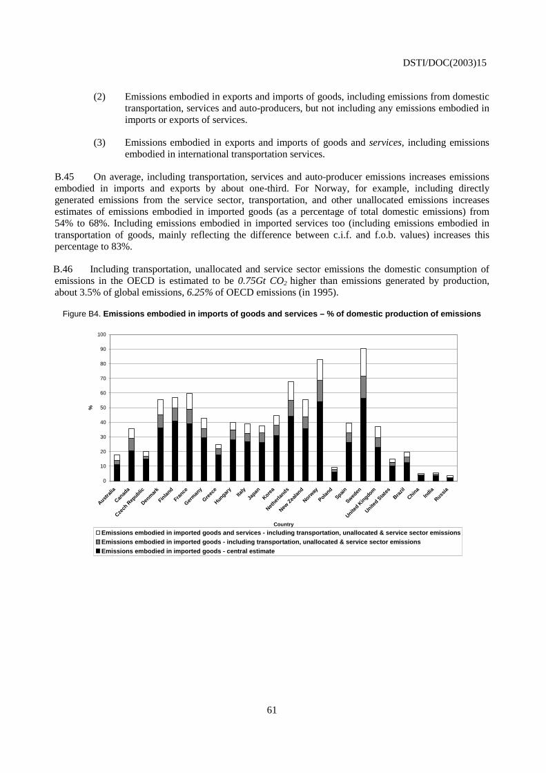
DSTI/DOC(2003)15
61
(2) Emissions embodied in exports and imports of goods, including emissions from domestic transportation, services and auto-producers, but not including any emissions embodied in imports or exports of services.
(3) Emissions embodied in exports and imports of goods and services, including emissions embodied in international transportation services.
B.45 On average, including transportation, services and auto-producer emissions increases emissions embodied in imports and exports by about one-third. For Norway, for example, including directly generated emissions from the service sector, transportation, and other unallocated emissions increases estimates of emissions embodied in imported goods (as a percentage of total domestic emissions) from 54% to 68%. Including emissions embodied in imported services too (including emissions embodied in transportation of goods, mainly reflecting the difference between c.i.f. and f.o.b. values) increases this percentage to 83%.
B.46 Including transportation, unallocated and service sector emissions the domestic consumption of emissions in the OECD is estimated to be 0.75Gt CO2 higher than emissions generated by production, about 3.5% of global emissions, 6.25% of OECD emissions (in 1995).
Figure B4. Emissions embodied in imports of goods and services – % of domestic production of emissions
0
10
20
30
40
50
60
70
80
90
100
Austra
lia
Canad
a
Czech
Rep
ublic
Denm
ark
Finlan
d
France
Germ
any
Greec
e
Hungary
Italy
Japan
Korea
Nether
lands
New Z
ealan
d
Norway
Poland
Spain
Sweden
United K
ingdom
United S
tate
s
Brazil
China
India
Russia
Country
%
Emissions embodied in imported goods and services - including transportation, unallocated & service sector emissionsEmissions embodied in imported goods - including transportation, unallocated & service sector emissionsEmissions embodied in imported goods - central estimate
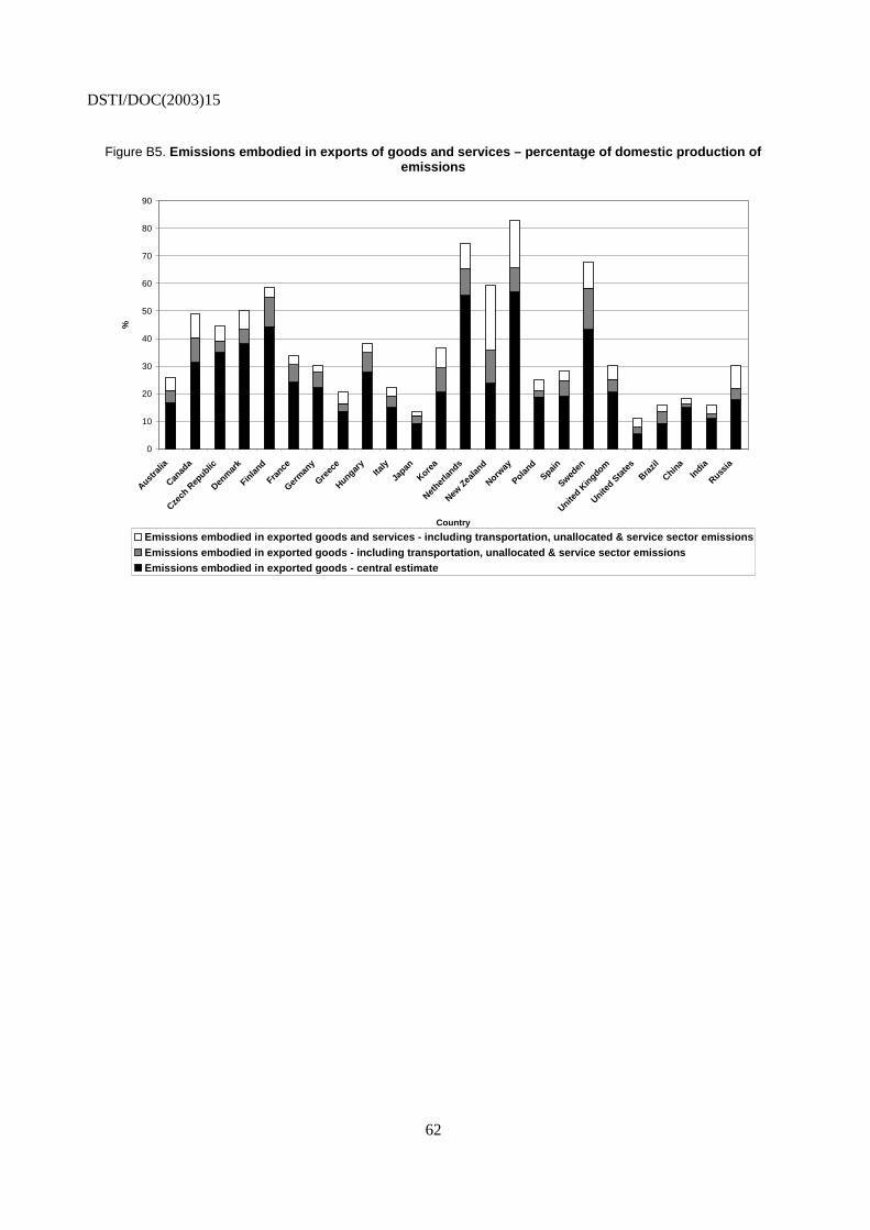
DSTI/DOC(2003)15
62
Figure B5. Emissions embodied in exports of goods and services – percentage of domestic production of emissions
0
10
20
30
40
50
60
70
80
90
Austra
lia
Canad
a
Czech
Rep
ublic
Denm
ark
Finlan
d
France
Germ
any
Greec
e
Hungary
Italy
Japan
Korea
Nether
lands
New Z
ealan
d
Norway
Poland
Spain
Sweden
United K
ingdom
United S
tate
s
Brazil
China
India
Russia
Country
%
Emissions embodied in exported goods and services - including transportation, unallocated & service sector emissionsEmissions embodied in exported goods - including transportation, unallocated & service sector emissionsEmissions embodied in exported goods - central estimate
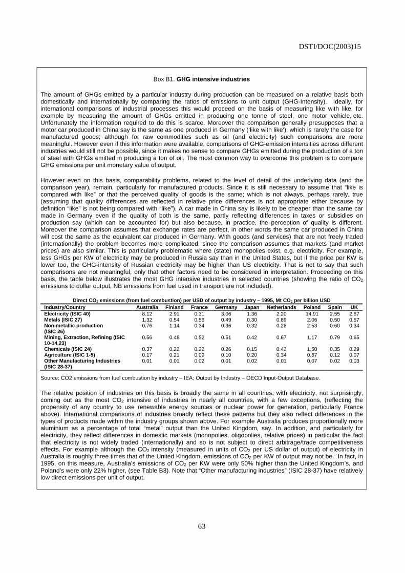
DSTI/DOC(2003)15
63
Box B1. GHG intensive industries
The amount of GHGs emitted by a particular industry during production can be measured on a relative basis both domestically and internationally by comparing the ratios of emissions to unit output (GHG-Intensity). Ideally, for international comparisons of industrial processes this would proceed on the basis of measuring like with like, for example by measuring the amount of GHGs emitted in producing one tonne of steel, one motor vehicle, etc. Unfortunately the information required to do this is scarce. Moreover the comparison generally presupposes that a motor car produced in China say is the same as one produced in Germany (‘like with like’), which is rarely the case for manufactured goods; although for raw commodities such as oil (and electricity) such comparisons are more meaningful. However even if this information were available, comparisons of GHG-emission intensities across different industries would still not be possible, since it makes no sense to compare GHGs emitted during the production of a ton of steel with GHGs emitted in producing a ton of oil. The most common way to overcome this problem is to compare GHG emissions per unit monetary value of output.
However even on this basis, comparability problems, related to the level of detail of the underlying data (and the comparison year), remain, particularly for manufactured products. Since it is still necessary to assume that “like is compared with like” or that the perceived quality of goods is the same; which is not always, perhaps rarely, true (assuming that quality differences are reflected in relative price differences is not appropriate either because by definition “like” is not being compared with “like”). A car made in China say is likely to be cheaper than the same car made in Germany even if the quality of both is the same, partly reflecting differences in taxes or subsidies on production say (which can be accounted for) but also because, in practice, the perception of quality is different. Moreover the comparison assumes that exchange rates are perfect, in other words the same car produced in China will cost the same as the equivalent car produced in Germany. With goods (and services) that are not freely traded (internationally) the problem becomes more complicated, since the comparison assumes that markets (and market prices) are also similar. This is particularly problematic where (state) monopolies exist, e.g. electricity. For example, less GHGs per KW of electricity may be produced in Russia say than in the United States, but if the price per KW is lower too, the GHG-intensity of Russian electricity may be higher than US electricity. That is not to say that such comparisons are not meaningful, only that other factors need to be considered in interpretation. Proceeding on this basis, the table below illustrates the most GHG intensive industries in selected countries (showing the ratio of CO2
emissions to dollar output, NB emissions from fuel used in transport are not included).
Direct CO2 emissions (from fuel combustion) per USD of output by industry – 1995, Mt CO2 per billion USD Industry/Country Australia Finland France Germany Japan Netherlands Poland Spain UK Electricity (ISIC 40) 8.12 2.91 0.31 3.06 1.36 2.20 14.91 2.55 2.67 Metals (ISIC 27) 1.32 0.54 0.56 0.49 0.30 0.89 2.06 0.50 0.57 Non-metallic production (ISIC 26)
0.76 1.14 0.34 0.36 0.32 0.28 2.53 0.60 0.34
Mining, Extraction, Refining (ISIC 10-14,23)
0.56 0.48 0.52 0.51 0.42 0.67 1.17 0.79 0.65
Chemicals (ISIC 24) 0.37 0.22 0.22 0.26 0.15 0.42 1.50 0.35 0.29 Agriculture (ISIC 1-5) 0.17 0.21 0.09 0.10 0.20 0.34 0.67 0.12 0.07 Other Manufacturing Industries (ISIC 28-37)
0.01 0.01 0.02 0.01 0.02 0.01 0.07 0.02 0.03
Source: CO2 emissions from fuel combustion by industry – IEA; Output by Industry – OECD Input-Output Database.
The relative position of industries on this basis is broadly the same in all countries, with electricity, not surprisingly, coming out as the most CO2 intensive of industries in nearly all countries, with a few exceptions, (reflecting the propensity of any country to use renewable energy sources or nuclear power for generation, particularly France above). International comparisons of industries broadly reflect these patterns but they also reflect differences in the types of products made within the industry groups shown above. For example Australia produces proportionally more aluminium as a percentage of total “metal” output than the United Kingdom, say. In addition, and particularly for electricity, they reflect differences in domestic markets (monopolies, oligopolies, relative prices) in particular the fact that electricity is not widely traded (internationally) and so is not subject to direct arbitrage/trade competitiveness effects. For example although the CO2 intensity (measured in units of CO2 per US dollar of output) of electricity in Australia is roughly three times that of the United Kingdom, emissions of CO2 per KW of output may not be. In fact, in 1995, on this measure, Australia’s emissions of CO2 per KW were only 50% higher than the United Kingdom’s, and Poland’s were only 22% higher, (see Table B3). Note that “Other manufacturing industries” (ISIC 28-37) have relatively low direct emissions per unit of output.
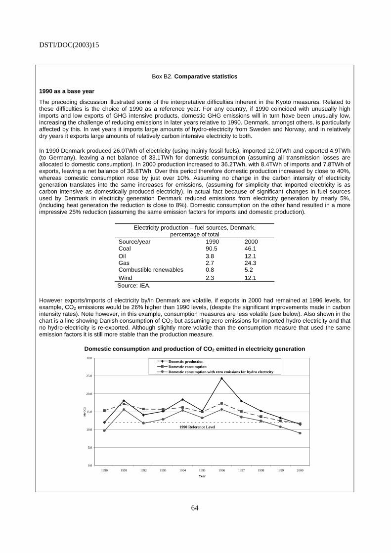
DSTI/DOC(2003)15
64
Box B2. Comparative statistics
1990 as a base year
The preceding discussion illustrated some of the interpretative difficulties inherent in the Kyoto measures. Related to these difficulties is the choice of 1990 as a reference year. For any country, if 1990 coincided with unusually high imports and low exports of GHG intensive products, domestic GHG emissions will in turn have been unusually low, increasing the challenge of reducing emissions in later years relative to 1990. Denmark, amongst others, is particularly affected by this. In wet years it imports large amounts of hydro-electricity from Sweden and Norway, and in relatively dry years it exports large amounts of relatively carbon intensive electricity to both.
In 1990 Denmark produced 26.0TWh of electricity (using mainly fossil fuels), imported 12.0TWh and exported 4.9TWh (to Germany), leaving a net balance of 33.1TWh for domestic consumption (assuming all transmission losses are allocated to domestic consumption). In 2000 production increased to 36.2TWh, with 8.4TWh of imports and 7.8TWh of exports, leaving a net balance of 36.8TWh. Over this period therefore domestic production increased by close to 40%, whereas domestic consumption rose by just over 10%. Assuming no change in the carbon intensity of electricity generation translates into the same increases for emissions, (assuming for simplicity that imported electricity is as carbon intensive as domestically produced electricity). In actual fact because of significant changes in fuel sources used by Denmark in electricity generation Denmark reduced emissions from electricity generation by nearly 5%, (including heat generation the reduction is close to 8%). Domestic consumption on the other hand resulted in a more impressive 25% reduction (assuming the same emission factors for imports and domestic production).
Electricity production – fuel sources, Denmark, percentage of total
Source/year 1990 2000 Coal 90.5 46.1 Oil 3.8 12.1 Gas 2.7 24.3 Combustible renewables 0.8 5.2 Wind 2.3 12.1
Source: IEA.
However exports/imports of electricity by/in Denmark are volatile, if exports in 2000 had remained at 1996 levels, for example, CO2 emissions would be 26% higher than 1990 levels, (despite the significant improvements made in carbon intensity rates). Note however, in this example, consumption measures are less volatile (see below). Also shown in the chart is a line showing Danish consumption of CO2 but assuming zero emissions for imported hydro electricity and that no hydro-electricity is re-exported. Although slightly more volatile than the consumption measure that used the same emission factors it is still more stable than the production measure.
Domestic consumption and production of CO2 emitted in electricity generation
1990 Reference Level
0.0
5.0
10.0
15.0
20.0
25.0
30.0
1990 1991 1992 1993 1994 1995 1996 1997 1998 1999 2000
Year
Mt C
O2
Domestic productionDomestic consumptionDomestic consumption with zero emissions for hydro electrcity

DSTI/DOC(2003)15
65
This example well illustrates the problems that can be incurred when focusing exclusively on domestic emissions alone. That is not to say that the choice of a reference year is in itself a bad idea, merely that emissions reductions targets based on domestic production can be acutely sensitive to the choice of reference year, and it is important to recognise that this presents difficulties whether emissions in the reference year were unusually low or high. Annex 1 transition economies are a good example of the latter. These economies experienced severe recessions after 1990, and the break-up of the Soviet Bloc. Indeed even in 2000 Russian GDP in real terms was one-third lower than it was in 1990, and the picture is little different for GHG emissions. Most forecasts predict that it will be some considerable time before the Russian economy returns to 1990 GDP levels and indeed the expectation is that by 2008-12, Russian GHG emissions will be considerably lower than the targets set out in the Kyoto Protocol. The difference between the emissions target and projected emissions can be, in theory, sold as “unused emissions entitlements” under the proposed emission credit trading system.