Trajectory optimization for musculoskeletal state estimation with IMU sensors

Ton van den BogertMechanical Engineering Department

1 CSU Center for Human-Machine Systems 8/27/2019

Combination of two conference presentations

2

XVth International Symposium on3D Analysis of Human Motion

Manchester, UK, July 2018Herman J. Woltring memorial lecture

International Society of BiomechanicsAmerican Society of Biomechanics

Calgary, Canada, August 2019

J Rehab Res Devel 1980

Adv Eng Software 1986

1980

1986

1988

Herman Woltring (1943-1992)

4

5

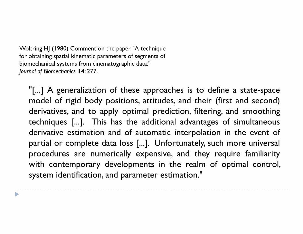
"[...] A generalization of these approaches is to define a state-spacemodel of rigid body positions, attitudes, and their (first and second)derivatives, and to apply optimal prediction, filtering, and smoothingtechniques [...]. This has the additional advantages of simultaneousderivative estimation and of automatic interpolation in the event ofpartial or complete data loss [...]. Unfortunately, such more universalprocedures are numerically expensive, and they require familiaritywith contemporary developments in the realm of optimal control,system identification, and parameter estimation."

Woltring HJ (1980) Comment on the paper "A technique for obtaining spatial kinematic parameters of segments of biomechanical systems from cinematographic data."Journal of Biomechanics 14: 277.

Is important in human movement, because measurements are often: inaccurate and noisy incomplete overcomplete & multiple modalities

Models can help (but aren't perfect...)

Optimal estimation can make use of all available measurements optimally combines measurements and model, with knowledge of how much to trust

each of them

Optimal estimation

PRINCIPLES

Rev. Thomas Bayes (1701-1761)Sir Isaac Newton (1643-1726)

Bayesian inferenceE: evidence (measurements)H: hypothesis (estimates of variables of interest)

Bayes' theorem:

Given the measurements E, which estimate H is best?Answer: find the H for which P(H | E) is highest

( | ) ( )( | ) ( ) ( | ) ( ) ( | )

( )P E H P H

P H E P E P E H P H P H EP E

ˆ argmax ( | ) ( )

HH P E H P H

H

( | ) ( )P E H P H

posterior probability

prior probability

H

Two approaches

10

Recursive (real time) Kalman filters, particle filters uses past measurements only

Trajectory optimization (not real time) uses past and future measurements

Both use the same "ingredients" process model observation model assumptions about how much to trust these models

Kalman filters: Q and R covariance matrices Trajectory optimization: effort weighting coefficient

recursiveestimation

trajectoryoptimization

Dynamic motion estimation

Nobody believes that this is actual human motion we know about Newton's laws of motion we know there is measurement error how do we estimate the actual motion?

mar

ker X

(mm

)

marker coordinatefrom optical motion capture

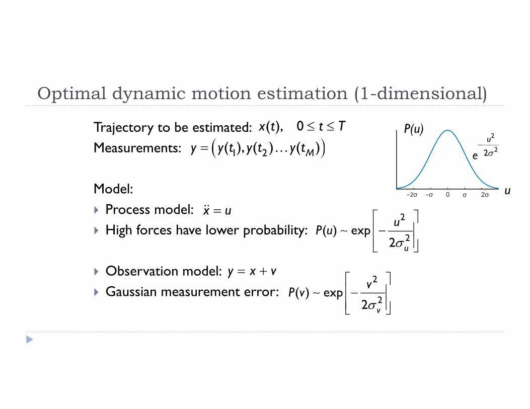
Optimal dynamic motion estimation (1-dimensional)

Trajectory to be estimated: Measurements:

Model: Process model: High forces have lower probability:

Observation model: Gaussian measurement error:

x u

y x v

2

2( ) exp

2 v

vP v

( ), 0x t t T

1 2( ), ( ) ( )My y t y t y t

2

2( ) exp

2 u

uP u

σ 2σ‒2σ ‒σ 0 u

2

22

u

e

P(u)

Optimal dynamic motion estimation (2)

   1 2 1 2( ) | | ( (, , ) )M MP ty y y y xy yx t P x P t

Probability that x(t) is the correct trajectory, given data y:

1 2 1 2

2

2

2 2 21 1 2 2 1 2

2 2 2

2

1

2

| ( ) | ( ) | ( ) ( ) ( ) ( )

( ) ( ) ( ) ( )~ exp exp exp exp

2 2 2 2

1exp

2

M M K

v v u u

v

P x t P x t P x t P x ty y y P x t P x t

y x t y x t x t x t

y

taking and factoring out constants:

 with  

2 2

21 1

22 2

21 0

1( ) ( )

2

~ exp ( ) ( ) ,

M K

i i ii iu

TMv

i ii u

x t x t

K

My x t p x t dt p

T

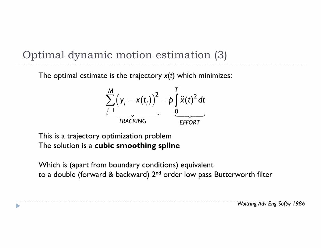
Optimal dynamic motion estimation (3)

The optimal estimate is the trajectory x(t) which minimizes:

2 2

1 0

( ) ( )TM

i ii

TRACKING EFFORT

y x t p x t dt

This is a trajectory optimization problemThe solution is a cubic smoothing spline

Which is (apart from boundary conditions) equivalentto a double (forward & backward) 2nd order low pass Butterworth filter

Woltring, Adv Eng Softw 1986

General, state space formulation

2 2

1 0

( ) ( )TM

i ii

TRACKING EFFORT

J y g x t p u t dt

Find state trajectory x(t) and control trajectory u(t) that minimize:

Subject to the process model: ( , , ) 0f x x u

Observation model: (sensor fusion) ( )y g x v

Cost function J: derived from Gaussian v and u & maximizing P(H|E)

Solution methods for trajectory optimization:Shooting (repeated simulation while iterating u(t) )Multiple Shooting (Mombaur)Direct Collocation (Ackermann & van den Bogert, J Biomech 2010)

trajectory smoothingand load sharing between muscles52 + 52 < 102 + 02

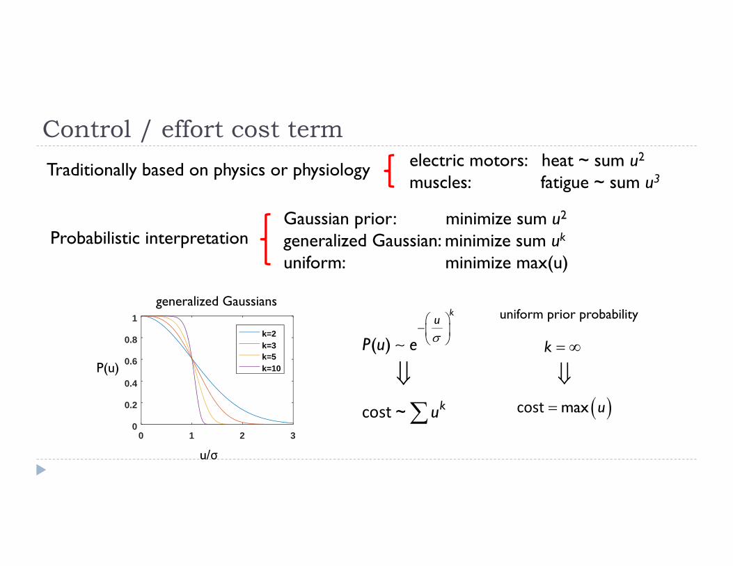
Control / effort cost term

Probabilistic interpretation

0 1 2 30

0.2

0.4

0.6

0.8

1k=2k=3k=5k=10

cost

( )

~

ku

k

P u e

u

u/σ

P(u)

cost

max

k

u

Traditionally based on physics or physiology electric motors: heat ~ sum u2

muscles: fatigue ~ sum u3

Gaussian prior: minimize sum u2

generalized Gaussian: minimize sum uk

uniform: minimize max(u)

uniform prior probabilitygeneralized Gaussians

Implicit musculoskeletal dynamics

van den Bogert et al., Procedia IUTAM 2011

, 0f(x, x u)

asvq

x

generalized coordinates

generalized velocities

projected fiber lengths

muscle activation states

max

( ) ( , ) ( )

( ) ( ) ( ) ( ) cos

1( )

TM

SEE M

SEE M FL CE FV CE PEE CE

act deact

F f f f

T T

q v

LM q v B q v F L q sq

0

F L q s a L L L

u ua u a

CE

refCErefCE

LsLsL

/cossin22

q1

q3

q2

downhill skiingstate estimation from low quality video data

Landing movement in downhill skiing

Data: low resolution video 2 panning cameras manual digitization 3D calibration in each frame

Nachbauer et al., J Appl Biomech 1996

Model and optimizationProcess model: planar 9-DOF skeleton 9-segment flexible skis 16 muscles ski boot stiffness ski-ground contact & friction x = (x1,x2...x82)

Observation model:g(x) = (q1,q2...q9) + v

Heinrich et al. Scand J Med Sci Sports 2014

2 2

1 0

( ) ( )TM

i ii

TRACKING EFFORT

J y g x t p u t dt

Cost function:

Solution:

, 0f(x, x u)

Kinematics of the landing movement

Heinrich et al. Scand J Med Sci Sports 2014

trajectory optimization

video data

LEFT RIGHT

trajectory optimization preserves high frequencies at impact

Other variables

left knee right knee

Ground reaction force

musclecontrols (u)

knee ligament forces

left

right

left right

walking and runningstate estimation from IMU data

Introduction

24

Inertial Measurement Unit (IMU) 3D accelerometer, 3D rate gyro, 3D magnetometer less expensive than optical motion capture not restricted to laboratory environment

Kinematic analysis sensor orientation from Kalman filter human inverse kinematics (Roetenberg et al., 2009)

Inverse dynamic analysis and muscle forces position drift no registration with force plate possible GRF prediction method (Karatsidis et al., 2019)

inverse kinematics, inverse dynamics, static optimization complete kinematic data needed

$36 - www.sparkfun.com

$12,000 - www.xsens.com

Trajectory optimization approach

25

Model of musculoskeletal dynamics: Find periodic trajectories x(t) and u(t) to minimize:

Potential advantages simultaneous estimation of kinematics, forces, muscle states solutions are dynamically consistent (obey physics and muscle physiology) can track raw unfiltered sensor data can work with incomplete data (and overcomplete data)

f(x,x,u) = 0

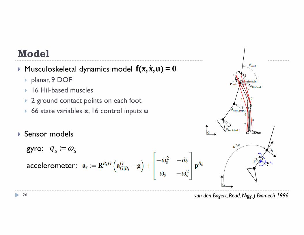
Model

26

Musculoskeletal dynamics model planar, 9 DOF 16 Hil-based muscles 2 ground contact points on each foot 66 state variables x, 16 control inputs u

Sensor models

gyro:

accelerometer:

f(x,x,u) = 0

:s sg

van den Bogert, Read, Nigg, J Biomech 1996

Evaluation study (J Biomech, in press)

27

10 subjects, 6 speeds (0.9 - 4.9 m/s) 10 trials at each speed 7 IMUs (sacrum, lateral thigh & shank, dorsal foot) Optical motion capture (OMC), force plates 2D joint angles and moments (Winter, 2009)

Ensemble averaging of data 100 points in average gait cycle, m ± σ

Trajectory optimization Comparison IMU vs. OMC results correlation coefficients RMS differences

Sensor signal tracking (running, one subject)

28

accel accel gyro

soft tissue artifactsare rejected

impact peaks aretracked

rightthigh sensor

rightshank sensor

rightfoot sensor

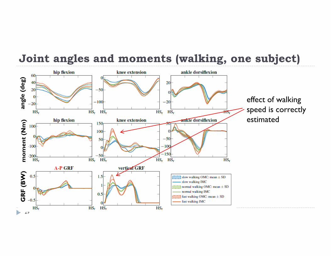
Joint angles and moments (walking, one subject)

29

effect of walking speed is correctly estimated

angl

e (d

eg)

mom

ent

(Nm

)G

RF

(BW

)

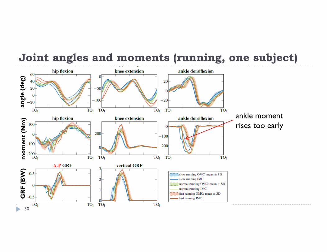
Joint angles and moments (running, one subject)

30

ankle moment rises too early

angl

e (d

eg)

mom

ent

(Nm

)G

RF

(BW

)

Correlations (all data, 10 x 6 x 100 points)

31

systematic overestimation

Discussion

32

Excellent correlation between IMU and OMC kinematics/kinetics (ρ > 0.9) Estimates of muscle forces and contraction/activation states consistent with typical EMG metabolic energy cost can be calculated from muscle state trajectories

Limitations computation speed: ~50 min for each of the 60 optimizations ankle moment overestimation, likely due to rigid foot model 2D analysis muscle load sharing is guided by optimization objective

Future work

33

Fewer sensors: minimal sensor set?

More sensors: EMG, foot pressure

Self-calibration Real time 3D analysis Validation for clinical and sports applications

Muscle forces

3Dresults

Bayes' theorem

( | ) ( )( | ) ( ) ( | ) ( ) ( | )

( )P B A P A

P A B P B P B A P A P A BP B