TRANSACTIONS ON AUTOMATION SCIENCE AND ENGINEERING 1

Automated Planning and Optimization of LumberProduction Using Machine Vision and Computed

TomographySuchendra M. Bhandarkar, Member, IEEE, Xingzhi Luo, Student Member, IEEE,

Richard F. Daniels and E. William Tollner

Abstract—An automated system for planning and optimizationof lumber production using Machine Vision and ComputedTomography (CT) is proposed. Cross-sectional CT images ofhardwood logs are analyzed using Machine Vision algorithms.Internal defects in the hardwood logs pockets are identified andlocalized. A virtual in silico 3-D reconstruction of the hardwoodlog and its internal defects is generated using Kalman filter-basedtracking algorithms. Various sawing operations are simulated onthe virtual 3-D reconstruction of the log and the resulting virtuallumber products automatically graded using rules stipulated bythe National Hardwood Lumber Association (NHLA). Knowledgeof the internal log defects is suitably exploited to formulate sawingstrategies that optimize the value yield recovery of the resultinglumber products. A prototype implementation shows significantgains in value yield recovery when compared to lumber process-ing strategies that use only the information derived from theexternal log structure. The system is intended as a decision aidfor lumber production planning and an interactive training toolfor novice sawyers and machinists in the lumber industry.

Index Terms—Automated Lumber Production, Lumber Pro-duction Optimization, Non-destructive Evaluation, AutomatedLumber Grading, Computed Tomography.

I. INTRODUCTION

The value of hardwood lumber is determined by the quan-tity, size and types of internal log defects such as knots, cracks,decay and other anomalies of tree growth that eventuallyappear on the lumber surfaces. Depending on the nature ofthe end utilization, each log is sawed to minimize the presenceof these internal defects on the resulting lumber surfaces. Inorder to achieve this goal, the internal defects within the logmust be accurately identified and localized prior to the sawingof the log. The knowledge of the nature and positions of theinternal log defects must then be exploited to determine alumber production strategy that maximizes the value and yieldof the resulting lumber product(s). In most sawmills, however,logs are processed into lumber based solely on external loginspection and knowledge of lumber grades with little or no

This work was supported in part by the US Department of Agriculturethrough an NRICGP grant (Award Number: 2001-35103-10049).

S.M. Bhandarkar and X. Luo are with the Department of ComputerScience, The University of Georgia, Athens, GA 30602-7404, USA (e-mails:suchi@cs.uga.edu, xingzhi@cs.uga.edu).

R.F. Daniels is with the Warnell School of Forest Resources,The University of Georgia, Athens, GA 30602-2152, USA (e-mail:ddaniels@smokey.forestry.uga.edu).

E.W. Tollner is with the Department of Biological and Agricultural Engi-neering, The University of Georgia, Athens, GA 30602-4435, USA (e-mail:btollner@engr.uga.edu).

information about the internal log defects and with inaccurateor incomplete geometric log data. This adversely affects theaccuracy of the lumber processing, resulting in suboptimallumber production where the potential value of logs is wasted.

Production of lumber is essentially a destructive and henceirreversible process; any loss in value yield due to incorrector suboptimal sawing is irrevocable. Given the low conversionefficiency of about 35% for conventional sawmills [16] andwith the rising costs of hardwood logs accounting for over80% of total production costs [17], improving the lumbervalue yield from hardwood logs has become imperative formany sawmills. Given the inherent limitations of externallog inspection, it is reasonable to assume that future gainsin lumber value yield will be achieved only by internal logscanning [7], [13], [17], [34].

Identification and localization of internal log defects areestimated to lead to potential gains of about 15%–18% inlumber value [7]. This represents a savings of over $2 billionfor the hardwood lumber industry in the United States [17],[25]. Forest products–based economies are increasingly de-pendent on getting the highest-value wood products from adeclining forest resource base. This results in disproportionateharvesting pressure on high-demand hardwood species suchas Hard Maple, Black Walnut, White Ash and Red Oak thatexhibit large differences in value between the highest andlowest lumber grades [33]. Environmental concerns and theecological need for maintaining biodiversity in forest ecosys-tems underscores the need to utilize as many hardwood speciesfor wood products as possible, to improve the efficiency inconverting low-grade logs into high-value lumber products,to reduce unnecessary wastage and to conserve valuable hard-wood forest resources. One way of achieving these goals is byidentification and localization of internal defects in hardwoodlogs and using this information to optimize the processing ofthe resulting lumber.

Studies of computed axial tomography (CAT or CT) andmagnetic resonance imaging (MRI) (also known as nuclearmagnetic resonance (NMR) imaging) for internal log de-fects [1], [2], [6], [13], [34] have demonstrated that the CTand MRI technologies available today can be used successfullyto image the internal features of logs. On account of theirinherent sensitivity to the water content of the imaged sample,MRI techniques are particularly well suited for detecting inter-nal features of logs, such as knots, reaction wood, wetwood,and gum spots, that are characterized by varying moisture

TRANSACTIONS ON AUTOMATION SCIENCE AND ENGINEERING 2

content in the underlying wood [6]. In CT images, on the otherhand, the grayscale value of a pixel is directly proportionalto the x-ray absorption which is then correlated with thematerial density at the pixel location [13]. Knots and moisturepockets are noted to have higher material density and/or highermoisture content than surrounding clear wood and are oftencharacterized by pixels with very high grayscale values in theCT image. Holes, cracks and decay pockets are void areasfilled with air or decayed wood and hence characterized bylow material density, resulting in corresponding CT imagepixels with very low grayscale values. Holes and decay pocketsusually have circular cross-sections and are typically short inlength whereas cracks are usually thin and long.

Although MRI is a more recent innovation, solid state CTscanners, capable of scanning rates close to 30 slices persecond, are fast approaching the speed necessary for real-timeproduction use in sawmills [17]. However, the computationalmethods for analyzing the CT images for internal defectsreliably and in real time, and exploiting the knowledge ofthe internal defects to determine optimal lumber processingstrategies are a challenging research topic and the subject ofthis paper.

In this paper we describe the design and implementationof a machine vision system for the automated planning andoptimization of lumber production from hardwood logs. Thepaper makes two significant contributions. First, a Kalmanfilter-based feature tracking framework is proposed to enablesimultaneous detection, localization and 3-D reconstructionof internal log defects in a manner that is computationallymuch more efficient than existing approaches. Second, detailedmathematical models and algorithms for lumber productionoptimization are proposed which exploit the knowledge of theinternal log defects to maximize the value yield recovery ofthe resulting lumber products. The system is intended as adecision aid for lumber production planning but could alsobe used as an interactive training tool for novice sawyers andmachinists, allowing them to practice various sawing strategieson virtual logs before working on real logs.

The remainder of the paper is organized as follows. Sec-tion II provides a brief review of previous work. Section IIIprovides an overview of the proposed system. Section IVprovides a detailed scheme for the detection, identificationand localization of internal defects such as holes, knots andcracks in a single CT image slice using a combination ofstructural and spectral features. Section V describes the 3-Dreconstruction of these internal defects using Kalman filter-based tracking algorithms. Section VI describes algorithms fordetermination of optimal lumber production strategies. SectionVII presents experimental results on real CT image data fromhardwood logs. Section VIII concludes the paper with anoutline for future work.

II. BRIEF LITERATURE REVIEW

Techniques for internal defect identification and classifica-tion in cross-sectional CT images of logs include gray-levelthresholding and binarization [13], [34], neural network-basedclassification [29], integration of shape and texture features

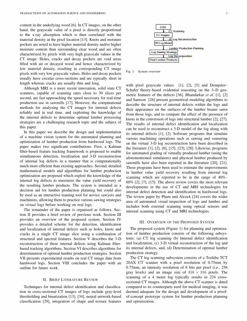
Fig. 1. System overview

with pixel grayscale values [1], [2], [5] and Dempster–Schafer theory-based evidential reasoning on the 3–D geo-metric features of the defects [36]. Bhandarkar et al. [1], [2]and Samson [26] present geometrical modeling algorithms todescribe the structure of internal defects within the logs andtheir appearance on the surfaces of the lumber beams sawnfrom those logs, and to compute the effect of the presence ofknots in the conversion of logs into structural lumber [2], [27].The results of internal defect identification and localizationcan be used to reconstruct a 3-D model of the log along withits internal defects [1], [2]. Software programs that simulatevarious machining operations such as sawing and veneeringon the virtual 3-D log reconstruction have been described inthe literature [1], [2], [8], [15], [23], [28]. Likewise, programsfor automated grading of virtually produced lumber (using theaforementioned simulators) and physical lumber produced bysawmills have also been reported in the literature [20], [21].These programs have been used to estimate the improvementsin lumber value yield recovery resulting from internal logscanning which are reported to be in the range of 40%–60% [2], [7], [15]. The above review covers the most relevantdevelopments in the use of CT and MRI technologies forinternal defect detection and identification in hardwood logs.The review paper by Pham and Alcock [24] covers the widerarea of automated visual inspection of logs and lumber andincludes both external scanning using optical sensors andinternal scanning using CT and MRI technologies.

III. OVERVIEW OF THE PROPOSED SYSTEM

The proposed system (Figure 1) for planning and optimiza-tion of lumber production consists of the following subsys-tems: (a) CT log scanning (b) Internal defect identificationand localization, (c) 3-D virtual reconstruction of the log andits internal defects, and, (d) Determination of optimal lumberproduction strategy.

The CT log scanning subsystem consists of a Toshiba TCT20AX CT scanner with a pixel resolution of 0.75mm by0.75mm, an intensity resolution of 8 bits per pixel (i.e., 256gray levels) and an image size of 316 × 316 pixels. Thescanning of a 4 meter log typically results in 224 cross-sectional CT images. Although the above CT scanner is datedcompared to its counterparts used for medical imaging, it wasdeemed adequate for the design and development of a proof-of-concept prototype system for lumber production planningand optimization.

TRANSACTIONS ON AUTOMATION SCIENCE AND ENGINEERING 3

Fig. 2. The flowchart of the defect detection system

The overall flowchart for the proposed defect detectionsubsystem is given in Figure 2. In the proposed subsystem,both structural (shape) and spectral (grayscale) features areincorporated in the detection and localization of internal logdefects in a single CT image slice. This addresses the limita-tions of conventional pixel-level thresholding or binarizationmethods which are limited in their classification accuracy,especially when confronted with overlapping pixel grayscalevalues from different defect classes, in spite of fairly sophisti-cated analysis of the grayscale histogram [8]. Furthermore, inthe proposed scheme, the processes of detection, localizationand 3-D reconstruction of internal defects are integrated acrossmultiple CT image slices within a single Kalman filter-basedfeature tracking framework. This is in contrast to most existingtechniques where the detection, identification and localizationof internal log defects are performed independently in eachCT or MR image slice and the 3-D reconstruction of thedefect is achieved via simple correspondence analysis acrossmultiple image slices using the defect shape, size and locationinformation [1], [2]. As a result, existing techniques arecomputationally inefficient and potentially unsuitable for real-time applications since the spatial coherence of the defectsalong the axial direction is not exploited. They are also error-prone, especially when dealing with defects with complex 3-Dshapes, since only two successive CT image slices are typicallyused to establish the correspondence.

In the proposed scheme, a Kalman filter [18] is used totrack the defect parameters continuously from one CT imageslice to the next by predicting the locations of the defects insuccessive slices. The algorithms for internal defect detectionand localization within a single CT image slice are used toinitialize the Kalman filter-based tracking algorithm. After adefect is detected and localized within a CT image slice,the tracking algorithm is used to detect and localize thedefect in successive CT image slices and also reconstruct itsgeometry in 3-D space. The net result is much faster detection,identification, localization and reconstruction of the internallog defects since only a local search within a fairly smallneighborhood of the predicted defect locations is entailed.

Given the 3-D reconstruction of the log and its internaldefects, the final subsystem determines the optimal lumberproduction strategy; one that maximizes the yield and grade

of the resulting lumber product. Mathematical models forcommonly performed sawing operations such as live sawing,cant sawing, grade sawing and secondary sawing are proposed.The optimal sawing strategy is determined by searching theparameter space of the sawing models using a dynamic pro-gramming algorithm. The dynamic programming algorithmdetermines the optimal spacings and orientations of the sawingplanes in order to maximize the value and yield of the resultinglumber products. A heuristic search algorithm is designed andshown to speed up the optimization process while providinga solution that is acceptably close to the optimal result. Anautomated lumber grading program that is compliant withthe National Hardwood Lumber Association (NHLA) gradingrules is designed to determine the grades of the (virtual)lumber products resulting from the simulation of the variousaforementioned sawing operations on the virtual 3-D logreconstruction.

IV. DETECTION OF DEFECTS IN A SINGLE CT IMAGE

Three major categories of defects are detected within asingle CT image slice, i.e., knots, holes and cracks, sincethey are known to greatly impact the grade and value of theresulting lumber.

A. Detection of Knots and the Outer Log Boundary

Knots are detected via analysis of the pixel grayscaleintensity in a local window surrounding the pixel as follows:

K(i, j) ={

1 if 1M2

∑(x,y)∈W (i,j) F (x, y) > Tk

0 otherwise(1)

where K(i, j) is the resulting binary image delineating theknots, W (i, j) is a window of predetermined size M × Mcentered at pixel (i, j), F (i, j) is a CT image slice of thelog and Tk is a predetermined threshold. A CT image slicecontaining a knot is shown in Figure 3(a) whereas the binaryimage resulting from the application of equation (1) is shownin Figure 3(b). A comparison of Figure 3(a) and Figure 3(b)shows that the application of equation (1) results in the erosionof the knot boundaries. Consequently, a morphological dilationoperation [30] is used to recover the knot boundaries asshown in Figure 3(c). The outer boundary of the log cross-section in a single CT image slice is also detected using thebinarization technique given in equation (1); however with asmaller window size (3×3 is typically adequate) and a smallerthreshold value (which is chosen to be slightly larger than thegrayscale value of a void area in the CT image).

B. Detection of Holes

Holes are actual void areas and appear as dark regions in theCT images with graylevels similar to those of the background.A simple thresholding scheme outlined in equation (2) is usedto classify the CT image pixels as holes.

K(i, j) ={

1 if F (i, j) < Th0 otherwise (2)

where Th is an empirically determined threshold value. Sinceholes are usually small in size and approximately round

TRANSACTIONS ON AUTOMATION SCIENCE AND ENGINEERING 4

(a) (b) (c)

Fig. 3. Result of knot detection: (a) CT image slice containing a knot, (b)Result of analysis of local graylevel pixel density, and (c) Extracted knotsafter dilation

(a) (b) (c) (d)

Fig. 4. Result of hole detection: (a) Input CT image, (b) Thresholded image,(c) Removal of cracks and valleys using erosion, and (d) Restoration of holesusing dilation

in shape, false holes, typically caused by small cracks orgrayscale valleys between successive rings, are removed byusing a combination of morphological erosion and dilationoperations on the thresholded result [30]. Figure 4 depicts theresults of the various stages of hole detection.

C. Detection of Cracks

A crack, in a CT image slice, is usually long and thin. Astraightforward grayscale-based binarization of the CT imageresults in either fragmentation of the detected cracks or toomany misclassifications of the regions denoting the grayscalevalleys between the annular rings as cracks. Since both, thegrayscale valleys and cracks are narrow and long, the grayscaledensity-based binarization technique (equation (1)) is not ableto separate them. However, cracks are typically perpendicularto the grayscale valleys and the local direction of a grayscalevalley can be estimated by approximating the grayscale valleysby concentric circles centered at the centroid of the log cross-section. This property is exploited in the crack detectionscheme.

The crack detection scheme is summarized as follows.The local linear structures resulting from cracks and valleysare first detected using Sobel-like edge operators and thenskeletonized using an edge thinning algorithm [10] as depictedin Figure 5(a). The points of intersection between the linesdefining the cracks and the lines defining the local structureof the valleys are represented as fork points within a localwindow (Figure 5(b)). Fork points that are distributed alongthe same crack-like feature are grouped using a greedy cluster-ing algorithm that exploits spatial connectivity and proximity(Figure 5(c)). A RANSAC-based line fitting algorithm [11]is used to determine the line segment characterizing a groupof fork points (Figure 5(d)). Crack-like features which areobserved to be parallel (within a certain angular threshold)to the local structure of the valleys are deemed to be spuriousand discarded. Given the parameters of the fitted line segment,

(a) (b) (c) (d)

Fig. 5. Result of crack detection: (a) Binary image resulting from the Sobel-like edge operators and edge thinning, (b) Result of fork detection, (c) Resultof fork grouping, and (d) Result of the RANSAC-based line fitting procedure

the actual crack pixels are determined using an iterative depth-first search procedure detailed in [3].

V. 3-D DEFECT RECONSTRUCTION USING THE KALMANFILTER

Since internal log defects are observed to exhibit spatialcoherence across several successive CT image slices, it ispossible to design computationally efficient algorithms for thedetection of knots, holes and cracks that take advantage ofthe defect attribute values predicted by the Kalman filter [18].Since knots, holes and cracks exhibit very different geometri-cal attributes in a 2-D image slice, different Kalman filteringmodels are proposed for each defect class. In addition, theouter boundary of the log cross-section is also detected andtracked across successive CT image slices in order to virtuallyreconstruct the entire log in 3-D space. The result is anintegrated and computationally efficient defect extraction and3-D defect reconstruction procedure that precludes the need toperform correspondence analysis independently for each pairof successive image slices.

A. 3-D Reconstruction of Knots and the Exterior Log Surface

The knots and the outer boundary of the log cross-sectionin a single CT image slice are simply encoded by using thepositions of their centroids and enumerating the pixels ontheir respective bounding contours. However, the raw contourpixels are not used directly as the tracked/predicted variablesin the Kalman filter model since the number of contourpixels varies significantly from one CT image slice to thenext and it is computationally inefficient to use too manytracked/predicted variables in the Kalman filter. Thus, for thepurpose of tracking, a knot defect or the exterior log boundaryin a single CT slice is encoded by its convex hull. The convexhull is defined by a small number of points and computed usingGraham’s algorithm [14]. A B-spline contour approximationalgorithm [12] is then used to determine the control points ofthe convex hull. The control points are used as the trackingparameters in the Kalman filtering model. The Kalman filteringmodel for the reconstruction of knots is depicted in Figure 6and is described as follows.

1) Initially, a knot defect area is detected in a single CTimage as described in Section IV-A.

2) The contour of the knot defect is extracted and its convexhull computed using Graham’s algorithm [14]. M B-spline control points are then used to approximate theconvex hull.

TRANSACTIONS ON AUTOMATION SCIENCE AND ENGINEERING 5

Fig. 6. An outline of the Kalman–Snakes based tracking method

3) The Kalman filter is applied to predict the velocity of theknot defect, where the term velocity denotes the rate atwhich the shape of the knot changes across successiveCT image slices. Let dx and dy denote the velocitycomponents along the x axis and y axis respectively. Lets denote the scale parameter in the time interval [t, t+1]such that s = 0 denotes the fact that the object size isunchanged in the time interval [t, t+ 1], s > 0 denotesthat the object size has increased and s < 0 denotes thatthe object size has shrunk in the same time interval. Ifat time t, the centroid of the convex hull is given by(cx, cy), and the velocity by (dx, dy, s), then for a point(x, y) on the convex hull at time t, its position (x′, y′)at time t+ 1 can be computed using equation (3).

x′ = x+ dx + s(x− cx)y′ = y + dy + s(y − cy) (3)

4) The predicted velocity (dx, dy, s) is used to estimatethe new position of the predicted convex contour usingequation (3). The updated convex contour is obtainedby using the predicted convex contour to initialize theSnakes contour fitting algorithm [19]. The Snakes con-tour fitting algorithm is used to search for the actualboundary of the knot in the new CT image slice.

5) Steps 2, 3 and 4 are repeated until all the CT imageslices are processed or the defect is too small in size tobe classified as a knot.

Since the above algorithm uses a combination of Kalmanfilter-based prediction and Snakes contour fitting, it is termedas the Kalman–Snakes algorithm [35]. The Kalman–Snakesalgorithm for reconstruction of the exterior log surface issimilar, except for some differences in how the convex hullpoints are generated. The detailed algorithms for convex hullgeneration, B-spline surface approximation and Kalman filter-based prediction are given in [4].

B. 3-D Construction of Holes and Cracks

The Kalman filter-based model for 3-D reconstruction ofcracks and holes is given by the following equations:

ξ−k+1 = ξ+k + qk (4)

Zk = ξ−k + vk (5)

where ξ is the tracking variable, Zk the measured value of thetracking variable, qk the random additive noise in the velocitytransition function which is modeled as zero-mean stationaryGaussian white noise with distribution N (0, Q0) and vk therandom additive noise in the velocity measurement functionwhich is also modeled as zero-mean stationary Gaussian whitenoise with distribution N (0, R0).

The contour of a hole is encoded by its bounding rectangle.The velocity of the center point of the rectangle is usedas the tracking variable (ξ = (ξx, ξy)T ) for holes. Given aprediction ξ−k+1, the new center point of the hole is computed.A rectangular image region centered on the predicted centerpoint is then subject to binarization using equation (2) andthe new location of the hole is obtained exactly using thetechnique for hole detection in a single CT image slice. Thus,the 3-D reconstruction of a hole is achieved by tracking thehole region across successive CT image slices.

For continuous crack detection, the CT images are firstbinarized using the scheme described in [3]. A crack defect isrepresented by the parameters (ρ, θ, x0, y0, l) where (x0, y0) isthe crack center and l the length of the line segment describingthe crack. The equation of the line describing the crack is givenby x cos θ + y sin θ = ρ where θ is the orientation angle ofthe line and ρ the perpendicular distance of the line from theorigin. The orientation angle θ is used as the tracking variableξ in the Kalman filter-based tracking model for a crack. Aftera crack is detected and extracted in the previous CT imageslices, its orientation angle in succeeding CT image slices ispredicted using equation (4). A fast crack localization schemedetailed in [4] is used to extract the crack in succeeding CTimage slices using the predicted orientation.

Note that in the above Kalman filter-based tracking ap-proach, it is not necessary to perform all the steps involvedin defect detection and localization in subsequent CT imageslices once they have been performed for the first CT imageslice in the image sequence. The defects that are detectedand localized are removed from further consideration. Theprocedures for defect detection and localization in a singleCT image slice (i.e., without defect tracking) are applied tothe remainder of the image to search for new defects.

C. Removal of False Defects and Insertion of Missing Defects

Spatial coherence is exploited to remove false defects andaccount for missing defects in the CT image slices. If a defectis detected in only one CT image slice, and no correspondingdefect is detected in k previous or k succeeding CT imageslices, where k is a predetermined threshold (in our case k =2), then the defect is deemed to have been caused by randomnoise and is removed from further consideration. Likewise,when the size of a defect is small, it is possible that it is notdetected in a single CT image slice. If a defect is detectedin CT image slices i − 1 and i + 1 but not in CT imageslice i, then it is necessary to verify whether or not the defect

TRANSACTIONS ON AUTOMATION SCIENCE AND ENGINEERING 6

Fig. 7. A typical lumber production system

exists in CT image slice i. The approximate position of thedefect in CT image slice i is computed via linear interpolationbetween its positions in CT image slices i − 1 and i + 1.The existence of the defect at the interpolated position in theCT image slice is verified by using the defect detection andlocalization procedure for a single CT image slice (i.e., withouttracking) but with relaxed threshold values.

VI. MATHEMATICAL MODELS FOR LUMBER PRODUCTIONOPTIMIZATION

Lumber production is essentially a decomposition processwhere the log is broken down to yield the desired lumberproducts. Given a 3-D model of the log, different sawingschemes can be used to decompose the log. Live sawing, cantsawing and grade sawing are primary sawing schemes [16]used to cut a log into flitches along sawing planes parallelto the axis of the 3-D cylindrical abstraction (i.e., the Z axisin our case) of the log (Figure 7). Secondary sawing [16] isused to further refine the flitches into higher quality boards(Figure 7). Given a board or a flitch, an automated gradingsystem is used to determine its value based on the grading rulesstipulated by the National Hardwood Lumber Association(NHLA) [22]. The grading system determines the value ofa flitch or board by classifying it into different grades basedon its quality which is determined by the type and size ofdefects that appear on the flitch or board surface. The size ofthe clear cutting (i.e., defect-free) areas and the size of thesurface defects are two important factors that determine thegrade of a flitch or board. The three dimensions of a board orflitch are termed as its length, width and thickness as illustratedin Figure 7. The goal of a computer-aided lumber productionplanning system is to determine the optimal sawing pattern inan appropriately chosen parameter space such that the value ofthe lumber products obtained from the log is maximized [31],[32].

A. Live Sawing

Consider a 3-D coordinate system associated with the 3-D cylindrical abstraction of a log such that the axis of thecylinder is parallel to the Z axis and the log cross-sectionslie in the XY plane. Live sawing is a straightforward sawingmethod where, for a given initial orientation of the saw in the

Fig. 8. Cutting range and sawing planes for live sawing

XY plane, the log is cut into flitches using sawing planes thatparallel to each other and parallel to the Z axis. Differentinitial orientations of the saw in the XY plane result indifferent values for the resulting lumber products. The goal informulating an optimal live sawing strategy is to determine thebest initial saw orientation in the XY plane and the optimalspacings between the mutually parallel sawing planes so asto maximize the value of the resulting lumber products. Inthe context of this paper, the term lumber or lumber productdenotes resulting flitches or boards depending on whetherthe sawing technique under discussion is a primary sawingtechnique or a secondary sawing technique respectively.

1) Formalization of Live Sawing: The variables used in theformalization of live sawing are defined below and illustratedin Figure 8. Figure 8 shows the projection of a cylindricallog on the XY plane. The outer (almost) elliptical boundarydenotes the projection of the larger cross-sectional end of thelog on the XY plane whereas the inner (almost) ellipticalboundary denotes the projection of smaller cross-sectional endof the log on the XY plane. Thus the log is modeled as acylinder with a monotonically tapering cross-section from oneend to the other. Note that this subsumes the special case ofa cylinder with uniform cross-section.• T = {T1, T2, ..., Tt}: a finite set of allowable lumber

thickness values in mm.• tmin: the minimum of the elements in T .• W = {W1,W2, ...,Ww}: a finite set of lumber width

values in mm.• wmin: the minimum of the elements in W .• c: cutting plane resolution (smallest separation between

two successive sawing planes) in mm.• K: the kerf of the sawing planes in mm. The kerf denotes

the finite thickness of the saw.• CR: the cutting range in mm.• N = bCR/cc the number of possible sawing planes that

can be accommodated within the sawing range.• θ: The initial orientation of the sawing plane as measured

in the XY plane (Figure 10). The value of θ ∈ [0o, 180o).It is assumed that the allowable lumber thickness values Tiand the sawing plane resolution c are integers. The sawingrange and other important parameters of the sawing surface inthe context of live sawing are computed as follows:

TRANSACTIONS ON AUTOMATION SCIENCE AND ENGINEERING 7

Determination of the Cutting Range: Given the initialorientation θ of the sawing plane, the cutting range for a log isfirst determined. Note that a valid piece of lumber must have aminimum width of wmin. Thus the cutting range is determinedby searching for the start and end locations of the sawingplane that results in a piece of lumber with valid width. Sincethe outer boundary of the smaller cross-sectional end of thelog is known, the cutting range for a given initial orientationθ of the sawing plane is determined by scanning from thecross-sectional boundary towards the cross-sectional centroidfrom two opposite ends as illustrated in Figure 8. A pair ofsawing planes within this range produces a piece of lumberwith a valid width value and prespecified thickness value. Tosimplify the analysis, it is assumed that the possible positionsof the sawing plane are discrete in steps of c mm (Figure 8).The value of c is assumed to be an integer and a reasonablevalue for c is 1 mm. N = bCR/cc represents the number ofpossible sawing planes that can be accommodated within thecutting range. The possible cutting planes are enumerated as1, 2, ..., N . It can be shown that the first sawing plane mustbe one of sawing planes between 1 and dtmin/ce, whereasthe last sawing plane must be one of sawing planes betweenN − dtmin/ce and N .

Cutting surface: For a given sawing plane, the appearanceof the resulting lumber surface (determined by the sizes anddistribution of the surface defects) determines the quality andprice of the resulting lumber product. The lumber surfacedata needed to evaluate the appearance of the lumber surfaceinclude the types, boundaries and sizes of the surface defectsand the outer log boundary.

Mathematical model for optimal live sawing: Inputs tothe optimal live sawing determination algorithm include thesawing orientation θ, T , W , various lumber price factors, andthe log data which includes the types, sizes, positions andorientations of the internal defects. The mathematical modelfor optimal live sawing can be simply represented by theobjective function:

Flive(log) = (Θ∗(log), S∗(Θ∗), V (S∗)) (6)

where Θ∗(log) is the optimal sawing orientation for a givenlog, S∗(Θ∗) is the optimal sawing pattern (determined by thelocations of the sawing planes) corresponding to the optimalsawing orientation Θ∗(log) and V (S∗) is the maximum valueof the lumber boards resulting from the optimal sawingpattern S∗(Θ∗) associated with the optimal sawing orientationΘ∗(log).

For a given value of θ, the cutting range CR(θ) can bedetermined as discussed earlier. Let C(θ) = {1, 2, ..., N} be afinite set of all possible positions of the sawing planes. S∗(θ) isthe optimal sawing pattern for the given sawing orientation θ.V (S(θ)) is the value of the resulting lumber (obtained using anautomated lumber grading algorithm) for a given the sawingpattern S(θ). A sawing pattern S(θ) = {s0, s1, ..., sn} is asubset of C(θ) that satisfies the following constraints:

(si − si−1 − dK/ce) · c ∈ T, for 1 ≤ i ≤ n (7)

1 ≤ s0 ≤ dtmin/ce (8)

Fig. 9. A feasible solution for live sawing

N − btmin/cc ≤ sn ≤ N (9)

A sawing pattern S(θ) that satisfies constraints (7)–(9) is adeemed to be a feasible sawing pattern for the log (Figure 9).Suppose the lumber generated by the sawing planes si−1

and si is of value vi. Let v = (v1, v2, ..., vn) be an n-vector describing the values of the lumber pieces generatedby the sequence of sawing planes S(θ) = {s0, s1, . . . , sn}.For S(θ) ⊂ C(θ), define V (S(θ)) =

∑j∈S(θ) vj to be the

total lumber value associated with the sawing pattern S(θ).In practical situations, constraint (7) is relaxed since forcinga lumber surface containing lots of defects into the finallumber product may result in lowering its overall value. Thusconstraint (7) is relaxed to the following pair of constraints:

(si − si−1 − dK/ce) · c ∈ T, for 1 ≤ i ≤ n (10)

or(si − si−1 − dK/ce) · c < tmin (11)

Thus, when constraint (11) is satisfied, a portion of the lumberbetween sawing surfaces si−1 and si is omitted from the finallumber product without lowering its value. Suppose ζ(θ) isa collection of subsets of C(θ), wherein each subset satisfiesthe sawing constraints (8) and (9) and, either constraint (10) orconstraint (11). Then the problem of determining the optimalsawing pattern is one of combinatorial optimization given by:

S∗(θ) = arg(max {v(S(θ)) : S(θ) ∈ ζ(θ)}) (12)

This combinatorial optimization problem can be easily solvedusing a dynamic programming algorithm [9].

The Dynamic Programming Algorithm: Function s∗(i) isdefined as the optimal sawing pattern for the portion of the logbetween sawing planes 1 and i and v∗(i) is the correspondingoptimal value of the lumber produced. Let g(i, j) be the valueof the lumber by the sawing planes i through j. It is obviousthat v∗(i) ≥ v∗(i− 1) and v∗(k) = 0, s∗(k) = Φ (where Φ isthe empty set) for all k < tmin/c. When the values of v∗(k)and s∗(k) for all k ≤ i are known, then

v∗(i+ 1) = maxj∈[0,t]

( (v∗(i+ 1− Tj/c− dK/ce)

+ g(i+ 1− Tj/c, i+ 1))) (13)

TRANSACTIONS ON AUTOMATION SCIENCE AND ENGINEERING 8

where dK/ce, the kerf size, is the minimum gap betweentwo sawing surfaces. Note that T0 = 0 when j = 0.This means that when j = 0, then the additional piece oflumber defined by the sawing surfaces (i, i + 1) does notincrease the maximum value of the overall generated lumberat point i + 1. Thus this piece of lumber is simply ignored,but may be reconsidered at a later point in the optimizationprocess. The relaxation of constraint (7) to constraint (10) orconstraint (11) makes it possible to discard some portion ofthe lumber that contains too many defects. Equation (13) inconjunction with constraints (8), (9) and either constraint (10)or constraint (11) results in the standard dynamic programmingalgorithm. Suppose j∗ results in the optimal value of v∗(i+1),then

s∗(i+1) = s∗(i+1−Tj∗/c−K/c∗)∪{i+1−Tj∗/c∗} (14)

In summary, the dynamic programming algorithm firstgenerates the initial values v∗(k) for k ≤ Tmin/c wherev∗(k) = 0, s∗(k) = Φ for k < Tmin/c and v∗(k) =g(1, k),s∗(k) = {k} for k = Tmin/c. Thereafter for eachi > Tmin/c, equations (13) and (14) are used iteratively toupdate v∗(i) and s∗(i) for all values of i. Finally, s∗(N) andv∗(N) correspond to S∗(θ) and V (S∗(θ)) in the objectivefunction Flive for a given value of the sawing orientation θ.

2) Live Sawing Algorithm: In the previous section, a dy-namic programming algorithm was designed to determineS∗(θ) and V ∗(θ) for a given value of the sawing orientationθ. However, to optimize the objective function Flive(log), theoptimal sawing orientation Θ∗ also needs to be determined. Areasonable heuristic would be to examine the major axes of allthe various internal log defects and if the internal defects areobserved to share a common major axis (within a prespecifiederror threshold) then the sawing orientation is chosen to bealong the common major axis (Figure 10(a)). This heuristictends to cluster the surface defects on a few lumber surfaces.Alternatively, one can perform an exhaustive search for Θ∗ in[0, 180) in discrete steps where the step size is determined bythe angular resolution of the saw (typically 2◦ or 4◦) as shownin Figure 10(b).

The exhaustive search method to optimize the objectivefunction, Flive(log) = (Θ∗(log), S∗(Θ∗), V (S∗)) can besummarized as:

1) For each sawing orientation θ ∈ [0, 180)a) Determine the cutting range CR. Let N =bCR/cc.

b) Run the dynamic programming algorithm to deter-mine and output the optimal sawing pattern S∗(θ)and the corresponding lumber value V (S∗)

2) Determine the optimal sawing orientation Θ∗ such thatV (S∗(Θ∗)) is maximized. Output Θ∗, S∗(Θ∗) andV (S∗).

In order to determine the computational complexity of theexhaustive search algorithm, we define tcr to be the time takento compute the cutting range CR, tcs to be the time taken toconstruct a cutting surface, tg to be the time taken to determineg(i, j) for each pair (i, j). At each step i, g(i, j) needs to becomputed |T | times where |T | is the cardinality of set T and

(a) heuristic

(b) exhaustive

Fig. 10. Sawing orientation selection

there are N steps in all. Therefore, for each value of the sawingorientation θ, the execution time is given by

Time(S∗(θ)) = tcr +N × tcs +N × |T | × tg (15)

in which, (.) denotes the average, because in practice Nvaries with the angular orientation θ, and tg also varies fordifferent (i, j) values in g(i, j). We define the parametertsg = tcs + |T | × tg . Thus the expression for Time(S∗(θ))can be simplified as Time(S∗(θ)) = tcr + N × tsg . We cansee that for a given sawing orientation, the execution time isroughly proportional to the cutting range. This confirms ourintuition that the larger the log diameter, the longer it takes todetermine the resulting lumber value.

In the case of exhaustive search, the total number of angularorientations explored is n = R/δθ, where δθ is the searchresolution for the sawing orientation. R is the search rangefor the sawing orientation and is 180◦. The execution time forthe exhaustive search is given by:

Time(Flive(log)) = R/δθ · (tcr +N × tsg) (16)

Instead of exhaustively searching the entire range of sawingorientations with a fixed angular resolution, one can performa coarse-to-fine search by initially searching the entire rangeof sawing orientations at coarse angular resolution and subse-quently narrowing down the search range while simultaneouslyincreasing the angular resolution (decreasing ∆).

Consider a class of objective functions given by:

F ∗(ζ) = maxζ∈R

(F (ζ)) (17)

where the goal is to determine the maximum value of F (ζ) andthe corresponding value of ζ. Function F (ζ) is known and Ris a range of ζ and is denoted by [A,B]. The minimum searchresolution δ for the parameter ζ is also known. The exhaustive

TRANSACTIONS ON AUTOMATION SCIENCE AND ENGINEERING 9

search algorithm, explores all possible values of ζ at a givenresolution and guarantees that the optimal value of F ∗(ζ)can be determined at that resolution. However, the exhaustivesearch algorithm is computationally inefficient. The proposedtwo-step coarse-to-fine algorithm is termed as Algorithm 1and is summarized below:Algorithm 1

1) Start with an initial angular resolution ∆ (where ∆ > δ),initial range R = [A,B] (where A = 0◦ and B = 180◦)and starting centroid c = (A+B)/2.

2) Search for the optimal value F ∗(ζ) and correspondingζ∗ for the given values of centroid c, angular resolution∆ and range R.

3) Set c = ζ∗, R = [ζ∗ − ∆/2, ζ∗ + ∆/2] and ∆ = δ.Perform step 2) again to determine the optimal valueF ∗(ζ) and the corresponding argument ζ∗ at resolutionδ.

The above two-step coarse-to-fine algorithm runs for R/∆+∆/δ iterations whereas the exhaustive search algorithm runsfor R/δ iterations in order to determine the optimal valueF ∗(ζ). When ∆ =

√Rδ, the two-step coarse-to-fine algorithm

runs for 2√R/δ iterations. For example, for δ = 2 and

∆ = 16 the two-step coarse-to-fine live sawing algorithm takes19 iterations whereas the exhaustive search algorithm takes 90iterations. The two-step coarse-to-fine algorithm could resultin a suboptimal result since not all possible values of theobjective function F are examined. However, our experimentalresults (Section VII) show that the value of F obtained usingthe two-step coarse-to-fine algorithm is nevertheless close tothe optimal value.

The computation time for optimal live sawing using Algo-rithm 1 for a given log is:

Time(Flive(log)) = 2√R/δθ · (tcr +N × tsg) (18)

whereas the computation time for optimal live sawing usingexhaustive search is:

Time(Flive(log)) = R/δθ · (tcr +N × tsg) (19)

B. Cant Sawing

The cant sawing algorithm is based on live sawing. Cantsawing breaks a log into three portions along the initial sawingorientation (Figure 11). Portions 1 and 3, at the extremities ofthe log cross-section, are subject to live sawing along the initialsawing orientation whereas portion 2 in the center of the logcross-section is subject to live sawing with the sawing planesorthogonal to the initial sawing orientation. Thus, in additionto determining the best initial sawing orientation, the optimalpositions of the two breakdown planes, denoted by l1 and l2in Figure 11 also need to be determined in order to arrive atthe optimal cant sawing strategy.

The objective function for cant sawing can be expressed as:

Fcant(log) = (Θ∗(log), L∗1(Θ∗), L∗2(L∗1), V (L∗1, L∗2),

S∗1 (L∗1), S∗2 (L∗1, L∗2), S∗3 (L∗2)) (20)

That is, in the case of cant sawing, the objective is to (a)determine the optimal sawing orientation Θ∗, (b) determine the

Fig. 11. Cant Sawing

locations of the sawing planes L∗1 and L∗2 for this orientation,and (c) determine the corresponding optimal lumber valueV (L∗1, L

∗2) and the corresponding sawing patterns S∗1 (L∗1),

S∗2 (L∗1, L∗2), and S∗3 (L∗2) for portions 1, 2 and 3 of the log

respectively (Figure 11). Note that for a given value of L1, anoptimal value for L2 can be determined; thus L2 is directlydependent on L1.

As in the case of live sawing, given a sawing orientationθ, the cutting range CR and the maximum number of sawingplanes N = bCR/cc can be determined. The variables l1 andl2 are used to define the locations of the sawing planes L1 andL2 respectively where 0 ≤ l1 < l2 < N (Figure 11). Whenvalues of l1 and l2 are determined, the optimal processing ofportions 1, 2 and 3 can be determined using the optimal livesawing algorithm described earlier (Figure 11). The optimallive sawing algorithm is applied to portions 1, 2 and 3 ofthe log with sawing orientations θ, 90− θ and θ respectively.Note that for portions 1 and 3 of the log, it is not necessary tocompute the cutting range CR, since N1 = l1 and N3 = N−l2respectively. However, for portion 2, each parameter needs tobe recomputed.

For a given log, an exhaustive search algorithm can be usedto determine the optimal values for θ, l1 and l2 as follows:

1) For each cutting orientation θ ∈ [0, 180)a) Determine the cutting range CR and N = bCR/ccb) For each l1 ∈ [0, N)

i) Run the dynamic programming algorithm onportion 1 and determine V ∗1 (l1), S∗1 (l1).

ii) For each value of l2 ≥ (l1 + 2K/c+Wmin/c).A) Run the dynamic programming algorithm

on portion 3 and determine V ∗3 (l2), S∗3 (l2).B) Determine the cutting range CR2 for por-

tion 2 and the corresponding value of N2.C) Run the dynamic programming algorithm

on portion 2 and determine V ∗2 (l1, l2),S∗2 (l1, l2).

iii) Determine the optimal value l∗2 , such thatV ∗2 (l1, l∗2) + V ∗3 (l∗2) is maximized. OutputV ∗2 (l1, l∗2), S∗2 (l1, l∗2) and V3 ∗ (l∗2), S∗3 (l∗2).

c) Determine the optimal value l∗1 such that V ∗1 (l∗1)+V ∗2 (l1, l2) + V ∗3 (l2) is maximized. Output V ∗1 (l∗1),

TRANSACTIONS ON AUTOMATION SCIENCE AND ENGINEERING 10

S∗1 (l∗1), V ∗2 (l∗1, l∗2), S∗2 (l∗1, l

∗2) and V ∗3 (l∗2), S∗3 (l∗2).

2) Determine the optimal cutting orientation θ∗, such that,L∗1 = L∗1(θ∗) and V ∗1 (l∗1) + V ∗2 (l1, l2) + V ∗3 (l2) ismaximized. Output θ∗, L∗1(θ∗), L∗2(L∗1), V ∗1 (l∗1), S∗1 (l∗1),V ∗2 (l∗1, l

∗2), S∗2 (l∗1, l

∗2) and V ∗3 (l∗2), S∗3 (l∗2).

Note that l2 = l1 + 2K/c + Wmin/c, because the width ofportion 2 of the log must be greater than Wmin. Howeverwe allow a special instance of cant sawing where l1 = l2(i.e., portion 2 is nonexistent); in which case cant sawing isequivalent to live sawing.

When θ is known, s∗(l1), v∗(l1) and s∗(l2), v∗(l2) can beprecomputed using the dynamic programming algorithm andstored for all possible values of l1 and l2. In this case, stepi) and step A) in the above algorithm need not be performedat each iteration. However in the case of portion 2, for eachpair (l1, l2), S∗2 (l1, l2) and V ∗2 (l1, l2) needs to be recomputed.Given a pair (l1, l2), the time to compute the optimal sawingpattern and resulting lumber value for portion 2 is given by:T (S∗(l1, l2)) = tcr + N2 · tsg . The total computation timeneeded to determine s∗1(l1) and s∗3(l2) for all l1 and l2 issimply given by Time(S∗1 (N)) + Time(S∗3 (N)) = tcr +N ·tsg . The total number of pairs (l1, l2) is given by (N/δl)2/2.In addition, if we let N2 = N , then the total computationtime for determination of optimal cant sawing for a specifiedorientation is given by

Time(L∗(θ)) = ((N/δl)/2 + 1)(tcr +N · tsg) (21)

The total time taken to compute the optimal cant sawing pat-tern using exhaustive search for determination of the optimalsawing orientation is given by

Time(Fcant(log)) = ((N/δl)2/2 + 1) ·R/δθ · (tcr +N · tsg)(22)

If the two-step coarse-to-fine strategy described in Algorithm1 is used to compute the optimal positions of sawing planesL1 and L2 and the optimal sawing orientation, then the totaltime taken to compute the optimal cant sawing pattern is givenby:

Time(Fcant(log)) = (2(N/δl) + 1) ·2√R/δθ · (tcr +N · tsg)

(23)

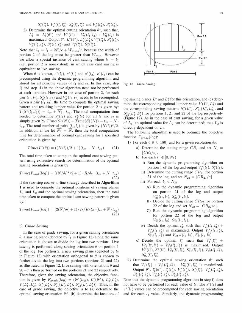
C. Grade Sawing

In the case of grade sawing, for a given sawing orientationθ, a sawing plane (denoted by l1 in Figure 12) along the sameorientation is chosen to divide the log into two portions. Livesawing is performed along sawing orientation θ on portion 1of the log. For portion 2, a new sawing plane (denoted by l2in Figure 12) with orientation orthogonal to θ is chosen tofurther divide the log into two portions (portions 21 and 22)as illustrated in Figure 12. Live sawing with orientations θ and90−θ is then performed on the portions 21 and 22 respectively.Therefore, given the sawing orientation, the objective func-tion is given by Fgrade(log) = (Θ∗(log), L∗1(Θ∗), L∗2(L∗1),V (L∗1, L

∗2), S∗1 (L∗1), S∗21(L∗1, L

∗2), S∗22(L∗1, L

∗2)). Thus, in the

case of grade sawing, the objective is to (a) determine theoptimal sawing orientation Θ∗, (b) determine the locations of

Fig. 12. Grade Sawing

the sawing planes L∗1 and L∗2 for this orientation, and (c) deter-mine the corresponding optimal lumber value V (L∗1, L

∗2) and

the corresponding sawing patterns S∗1 (L∗1), S∗21(L∗1, L∗2), and

S∗22(L∗1, L∗2) for portions 1, 21 and 22 of the log respectively

(Figure 12). As in the case of cant sawing, for a given valueof L1, an optimal value for L2 can be determined; thus L2 isdirectly dependent on L1.

The following algorithm is used to optimize the objectivefunction Fgrade(log):

1) For each θ ∈ [0, 180) and for a given resolution δθ.a) Determine the cutting range CR1 and set N1 =bCR1/cc.

b) For each l1 ∈ [0, N1)i) Run the dynamic programming algorithm on

portion 1 of the log and output V ∗1 (l1), S∗1 (l1).ii) Determine the cutting range CR21 for portion

21 of the log, and set N21 = bCR21/cciii) For each l2 < N21

A) Run the dynamic programming algorithmon portion 21 of the log and outputV ∗21(l1, l2), S∗21(l1, l2).

B) Decide the cutting range CR22 for portion22 of the log and set N22 = bCR22/cc.

C) Run the dynamic programming algorithmfor portion 22 of the log and outputV ∗22(l1, l2), S∗22(l1, l2).

iv) Decide the optimal l∗2 , such that V ∗21(l1, l∗2) +V ∗22(l1, l∗2) is maximized. Output V ∗21(l1, l∗2),S∗21(l1, l∗2) and V22 ∗ (l1, l∗2), S∗22(l1, l∗2).

c) Decide the optimal l∗1 such that V ∗1 (l∗1) +V ∗21(l∗1, l

∗2) + V ∗22(l∗1, l

∗2) is maximized. Output

V ∗1 (l∗1), S∗1 (l∗1), V ∗21(l∗1, l∗2), S∗21(l∗1, l

∗2), V ∗22(l∗1, l

∗2),

S∗22(l∗1, l∗2).

2) Determine the optimal sawing orientation θ∗ suchthat V ∗1 (l∗1) + V ∗21(l∗1, l

∗2) + V ∗22(l∗1, l

∗2) is maximized.

Output θ∗, l∗1(θ∗), l∗2(l∗1), V ∗1 (l∗1), S∗1 (l∗1), V ∗21(l∗1, l∗2),

S∗21(l∗1, l∗2), V ∗22(l∗1, l

∗2), S∗22(l∗1, l

∗2).

Note that the dynamic programming algorithm in step i) doesnot have to be performed for each value of l1. The s∗(l1) andv∗(l1) values can be precomputed for each sawing orientationand for each l1 value. Similarly, the dynamic programming

TRANSACTIONS ON AUTOMATION SCIENCE AND ENGINEERING 11

algorithm in step C) does not have to be performed for eachvalue of l2, given a value of l1. However, for portion 21 of thelog, all possible pairs of (l1, l2) values have to be considered.For portion 1 of the log, the computation time is tcr+N1 ·tsg ,For portion 21 of the log, there are N1/δl possible values forl1, therefore, the computation time is N1/δl · (tcr +N21 · tsg).For portion 22 of the log, there are N1/δl × N2/δ1 possiblevalues for (l1, l2) so the computation time is N1/δl×N2/δ1 ·(tcr +N22 · tsg). If we let N1 = N2 = N21 = N22 = N thenthe total computation time for determination of optimal gradesawing is

Time(Fgrade(log)) = (1+N/δl+(N/δl)2)·R/δθ·(tcr+N ·tsg)(24)

If the two-step coarse-to-fine strategy outlined in Algorithm1 is used to determine the optimal sawing plane positionsl1 and l2 and the optimal sawing orientation, then the totalcomputation time for determination of optimal grade sawing

is given by Time(Fgrade(log)) = (4(N/δl) + 2√N/δl + 1) ·

2√R/δθ · (tcr +N · tsg).

D. Secondary Sawing

In primary sawing (i.e., live sawing, cant sawing, gradesawing) slabs of wood termed as flitches are produced. Theseflitches are further processed to produce edged (cut length-wise) and trimmed (cut widthwise) pieces termed as boards(Figure 7). This procedure is called secondary sawing. Thepurpose of secondary sawing is to produce higher qualityboard products from flitches.

The parameters used in secondary sawing are the same asthose used in primary sawing. The viewing angle for the flitchis perpendicular to the surface of the lumber. The orientation ofthe sawing plane is fixed and is either parallel or perpendicularto the Z axis as illustrated in Figure 7. In primary sawing, theconstraints are primarily imposed on the lumber thickness T .In the case of secondary sawing, the constraints are imposedon the board width W and length L.

There is no concept of cutting range in the case of sec-ondary sawing. A flitch of width Wf , for a given sawingresolution c, is divided into N = bWf/cc sawing planes. Theobjective function for secondary sawing is Fsecond(flitch) =(S∗(flitch), V (S∗)), that is, given a flitch, determine theoptimal sawing pattern S∗ and corresponding maximum valueV (S∗). Note that there is no dependence on the sawing ori-entation which is fixed (unlike primary sawing). The dynamicprogramming procedure to optimize Fsecond(flitch) can bestated as follows:

Let s∗(i) to be the optimal sawing pattern for sawing planepositions from 1 to i for the given flitch and v∗(i) to be thecorresponding value. If v∗(k) and s∗(k) for all k ≤ i areknown, then

v∗(i+ 1) = maxj∈[0,W ]

( v∗(i+ 1− dWj/ce − dK/ce)

+g(i+ 1− dWj/ce, i+ 1)) (25)

where W = {W1,W2, . . . ,Wn} is the allowed set of widthvalues and g(i, j) is value of the portion of the board between

sawing planes i and j. As in the case of live sawing, dK/ce isthe kerf size which determines the minimum gap between twoboards. Note that the width Wj is used instead of the thicknessTj as in the case of primary sawing. As in the case of livesawing, the constraints on the sawing pattern S are relaxed i.e.,j can be 0 in which case W0 = 0. This means that if j∗ = 0,then the additional portion (i, i + 1) would not increase themaximum value of the log at point i + 1. This portion couldbe currently ignored, but could also be reconsidered at a laterpoint. The above constraint relaxation makes it possible todiscard some portion(s) of the flitch that contain(s) too manydefects.

If j∗ results in the best value v∗(i+ 1) then

s∗(i+1) = s∗(i+1−W ∗j /c−dK/ce)∪{i+1−W ∗j /c} (26)

Equation (26) defines a dynamic programming algorithm.The outputs s∗(N) and v∗(N) of the dynamic programmingalgorithm are the optimal sawing pattern S∗(log) and thecorresponding value V (S∗) respectively.

In secondary sawing, there is no need to generate thelumber surface for a sawing plane as in the case of primarysawing; it is sufficient to only check the appearance of defectson the top and bottom surface of the board. Therefore, thetime complexity of secondary sawing for a given flitch is:Time(Fsecond(flitch)) = N × w × tg , in which tg is thetime to determine the value of a given board.

A similar dynamic programming approach can be formu-lated to generate boards of allowable lengths resulting in a two-step dynamic programming algorithm. A flitch of width Wf

and length Lf for a given sawing resolution c, is divided intoNW = bWf/cc horizontal sawing planes and NL = bLf/ccvertical sawing planes. Let s∗(i, j) to be the optimal sawingpattern for the horizontal sawing plane positions from 1 to iand vertical sawing plane positions from 1 to j for the givenflitch, and v∗(i, j) to be the corresponding value. If v∗(k, l)and s∗(k, l) for all k ≤ i are known, then

v∗(i+ 1, j + 1) = maxk∈[0,W ](maxl∈[0,L]((v∗(i+ 1− dWk/ce − dK/ce,j + 1− dLl/ce − dK/ce)

+g(i+ 1− dWj/ce, i+ 1,j + 1− dLl/ce, j + 1)))) (27)

where L = {L1, L2, . . . , Ln} is the set of allowablelengths and g(i, j, k, l) is the value of the lumber betweenthe horizontal sawing planes (i, j) and vertical sawing planes(k, l).

E. Lumber Grading

Given a flitch or a board, a well-defined and systematicgrading system is essential to determine its value. An auto-mated grading subsystem is a critical component of an overallautomated lumber production planning system. The gradingprocess is that of classification of a board or flitch into oneof various grades based on its size and defect content andcomputation of its price based on the assigned grade and itssurface area. The most commonly used hardwood grading

TRANSACTIONS ON AUTOMATION SCIENCE AND ENGINEERING 12

rules are the ones promulgated by the National HardwoodLumber Association (NHLA) [22]. In practice, manual lumbergrading via application of the various NHLA rules is acomplicated process. Consequently, lumber companies usuallyhire trained professional lumber graders for this importanttask. In our automated lumber production planning system, anautomated lumber grading subsystem is implemented based oncompilation of the various NHLA grading rules.

Under the NHLA hardwood grading system, the gradeassigned to a hardwood board or flitch is based on the numberand sizes of clear/sound face cuttings that can be obtained froma board or flitch. A clear face cutting is a piece that is free ofdefects on one side except for minor seasoning checks. Thestandard NHLA grades in the order from highest to lowest areFirst and Second (FAS), Selects, Number 1 Common, Number2A and 2B Common, Number 3A Common and Number 3BCommon as shown in Figure 13. For example, FAS gradelumber is the best suited for high quality furniture, high qualityveneer, interior trim or molding. Some important terminologypertaining to lumber grading using the NHLA rules is givenas follows.

1) Lumber Grading Terminology:Surface measure: Surface measure (SM) is the surface areaof a board in square feet and is computed as follows:

SM = width(inches)× integer length(feet)÷ 12 (28)

In equation (28) the width of the board is measured in inches(including the fractional portion) whereas the length of theboard is measured in integral feet obtained via truncation ofthe actual length in feet. The result is expressed as an integerobtained via rounding of the product. For example, a flitch ofsize 6 7

16 inches × (10feet 9inches), has a surface measure ofSM = (6 7

16 × 10)/12 = 5.36 ≈ 5ft2.Poor side: One of the two surfaces of a flitch is considered asthe poor side. The poor side of the flitch is the one associatedwith a lower grade. If both sides have the same grade, thenthe surface with fewer cutting units is deemed the poor side.Cutting: A rectangular portion of a board or flitch. Differentgrades have different requirements on the quality, sizes andnumber of the resulting cuttings.Clear Cutting: A cutting without any visible surface defects.Sound cutting: A cutting with only certain allowed types ofvisible surface defects.Cutting Unit: Cutting unit (CU) is a unit of measure com-prising of a 1 inch width and a 1 foot length. The number ofcutting units associated with a cutting is computed as:

CU = [width (inches)+fraction]×[length (feet)+fraction](29)

For the sake of clarification consider the example board shownin Figure 14. The SM of the board is 10(in)× 11(feet)/12 =9.16 ≈ 9ft2. The number of cuttings is two as indicated bythe two rectangular boxes A and B in Figure 14. Since boththe cuttings are free of defects, they are deemed to be clearcuttings. The total number of cutting units associated with theboard is computed as: CU = (6.5in×7ft)+(3.5in×9ft) = 77

2) Grading Rules: Different lumber grades have differentrequirements with regard to the quality, sizes and number

Fig. 13. Grading Table

Fig. 14. Clear cutting units and grading of a board

of the resulting cuttings as shown in the grading table inFigure 13. For example, to qualify as grade FAS, a boardmust have a width greater than 6 inches, length between 8 feetand 16 feet. The FAS grade allows a total of at most SM/4cuttings to be used to determine the total number of clearcutting units. A cutting must be larger than 4 inches× 5 feetor 3 inches× 7 feet. The total number of clear cuttings unitsmust be at least 10/12× (SM ×12). For example, in the caseof the board shown in Figure 14 the required number of clearCUs is 10/12×9×12 = 90 for the board to be classified as FASgrade. If the maximum number of clear CUs obtained fromthe board is 77, as shown earlier, then this board cannot beclassified as FAS grade. However, it is possible to determinethe optimal locations of the cuttings that would enable theboard to be classified as FAS grade.

To determine the highest possible grade for a board, wefirst compute its surface measure (SM) and then the numberof cutting units (CUs). The required number of clear cuttingsis determined using the requirements displayed in Figure 13.Next, the maximum number of clear cutting units is deter-mined based on the locations of the defects as described below.

3) A Mathematical Model to Compute Clear Cutting Units:The width, length and the surface measure SM of a board orflitch are easily computed. The real difficulty lies in deter-mining the number and locations of the clear/sound cuttingssince the stipulated requirements on the number and sizes ofthe cuttings and the total number of cutting units (CUs) varieswith the grade. Therefore, to classify a board as belongingto a certain grade, the grading system needs to compute thenumber and sizes of the clear/sound cuttings and the totalnumber of CUs associated with the board and match thesewith the stipulated requirements for each grade as tabulated inthe grading table (Figure 13).

Suppose the length and width of the board are L and Wrespectively. The image of the board surface is divided into aL/rl ×W/rw grid as shown in Figure 15 where rw and rl

TRANSACTIONS ON AUTOMATION SCIENCE AND ENGINEERING 13

Fig. 15. The grid image used for determining the clear/sound cuttings

denote the dimensions of each grid cell along the width andlength respectively. The parameters rw and rl thus controlthe grid granularity or resolution. A finer grid resolutionincreases the computational complexity whereas a coarser gridresolution decreases the accuracy of the analysis. A grid cellp in the yth row and xth column is represented as p(x, y).Grid cell p1(x1, y1) is said to precede cell p2(x2, y2) if oneof the two conditions is satisfied:: (1) y2 > y1; (2) y2 = y1and x2 > x1. Two cells p1(x1, y1) and p2(x2, y2) where p1

precedes p2, define a rectangle with p1 and p2 as the end pointsof its diagonal. A grid cell p(x, y) is deemed to lie within therectangle when x1 ≤ x < x2 and y1 ≤ y < y2. Given alog and the 3D geometry and locations of its internal defects,the grid cells containing each defect can be determined. Toenhance the computational efficiency of the search for clearcuttings, the grid image is encoded using run-length codesalong both the x-direction and y-direction in the defect-freeregions.

The mathematical model for determining the optimal num-ber of clear cuttings is described below. The variables used inthis model are listed as follows.• Nc: the maximum number of allowable cuttings for a

certain grade. This value is determined using the gradingtable.

• S = {(wi, li)}, i = 1, ..., s: the minimum allowablesizes of the cuttings for a certain grade where the widthand length are expressed in grid units. These valuesare obtained from the grading table. Under the NHLAstandard, the value of s is usually small (1 or 2).

• Cu: The minimum number of clear cutting units allowedfor a certain grade. This value is also obtained from thegrading table.

Thus, given a board/flitch surface, the objective is to obtain themaximum number of clear cutting units under the constraintsof Nc and S. Therefore, the target function is represented asFcut = (C∗, CU(C∗)), where C∗ is the set of optimal cuttingsand CU(C∗) is the number of cutting units associated withC∗. The number of cuttings in C∗ is no larger than Nc. Thesize of each cutting in C∗ is no less than that of any elementin S.

A legal set of cuttings of a board is represented as anarray of nonoverlapping rectangles C = {cj(p1, p2)}, 1 ≤j ≤ c ≤ Nc, where c is the total number of cuttings. Forconvenience, let pj1 represent the first grid cell and pj2 thesecond grid cell that define rectangle cj(p1, p2) (note that

Fig. 16. Sorted legal cuttings

Fig. 17. Cutting graph

(pj1, pj2) defines the diagonal of the rectangle cj). A feasible

solution C to the cuttings determination problem satisfiesthe following conditions: (1) Rectangles ci and cj are non-overlapping for 1 ≤ i, j ≤ c; and (2) Rectangle pi1 precedesrectangle pj1 for 1 ≤ i < j ≤ c.

Given a board/flitch, all the legal cuttings are scanned andstored in an array C = {cj}. The array C is sorted based onthe coordinates of the first grid cell of each cutting as shown inFigure 16. A directed graph for array C is then constructed.The nodes of the graph are cuttings labeled based on theirorder in array C. Each node j in the graph is assigned a valueCU(cj) . Two non-overlapping nodes i and j in the graph,where i < j, are connected by a directed edge eij from nodei to node j. Two dummy nodes 0 and c+ 1 are added to thegraph. The value associated with nodes 0 and c+ 1 is 0. Forany node j in the graph, where 1 ≤ j ≤ c, there is an edgefrom node 0 to node j from node j to node c+1. The resultinggraph is shown in Figure 17 in which there are directed edgesfrom node 1 to nodes 4, 5, 6, 7 and 8, because cutting 1 inFigure 16 does not overlap with cuttings 4, 5, 6 and 7.

A path in the above graph is defined as a sequence of nodesp = 0, i1, i2, ..., ik, c+1, that satisfies the conditions 0 < i1 <i2 < ... < ik < c+1 and k ≤ Nc. The total number of cuttingunits associated with this path is given by

CU(p) =k∑j=1

CU(cij ) (30)

The optimal set of cuttings corresponds to the path p∗

which maximizes CU(p). A dynamic programming algorithmoutlined below is used to find the optimal path p∗:

(1) Initialization: C∗(0) = Φ and CU∗(0) = 0 for node 0where Φ is the empty set.(2) For each node i ∈ [1, c+ 1], compute

CU∗(i) = CU(i) + maxj∈p(i)

CU(j) (31)

where p(i) is the set of all nodes which have edges to nodei. C∗(i) = C(arg (maxj∈p(i) CU(j))) ∪ {ci}

TRANSACTIONS ON AUTOMATION SCIENCE AND ENGINEERING 14

Fig. 18. Flow chart of the grading system

(3) C∗ = C∗(c+ 1) is the optimal set of cuttings and CU∗ =CU∗(c + 1) is the corresponding optimal number of cuttingunits.

If the optimal number of cutting units CU∗ ≥ Cu for agiven grade, then the board/flitch surface can be classified asbelonging to that grade. The classification of a board/flitch sur-face proceeds from the highest grade FAS to the lowest grade3B COM. The values of C∗ and CU∗ are computed subjectto the constraints of each grade category and the board/flitchsurface assigned to the highest grade that it qualifies for.

4) Grading system: The flowchart of the overall gradingsystem is summarized in Figure 18. Given the two surfacesof a board or flitch, both surfaces are graded. Once thegrades of both surfaces determined, the final grade of theentire board/flitch is determined. The final grade of the entireboard/flitch is typically the lower of two surface grades. Afterthe final grade of a board/flitch is determined, the price of theboard/flitch is computed based on a pricing table. The pricingtable typically contains the cost per clear cutting unit for eachgrade category.

F. Lumber value determination

In practice, the lumber value is determined by its speciesgroup, its grade, its size (width, thickness and length) andmarket demand. The hardwood lumber grade is based on theappearance of the defects on lumber surfaces and determinedaccording to the NHLA rules [22]. The effect of the marketdemand factor can be typically represented by other factorsrelated to species, grade, volume and dimensions of thelumber. Thus the value of a piece of lumber v may be obtainedusing the following formula:

v = V PsPgPwPtPl (32)

where V is the lumber volume, Ps, the base price for a unitvolume of a certain lumber species, Pg , the price factor relatedto the lumber grade, and Pw, Pt and Pl the price factors related

TABLE ITHE LUMBER VALUE FACTOR: GRADE AND THICKNESS

Grade Pg thickness (mm) Pt

FAS 1100 (5, 10] 0.75Select 800 (10, 15] 0.8No1 Common 500 (15, 25] 1No2 Common 400 (25, 40] 1.1No3a Common 350 (40,60] 1.05

TABLE IITHE LUMBER VALUE FACTOR: LENGTH AND WIDTH

length (mm) Pl width (mm) Pw

(50,200] 0.7 (50, 100] 0.8(200, 400] 0.8 (100,150] 0.95(400, 800] 0.9 (150,250] 1

(800, 1000] 1 (250,350] 1.1(1000, 1200] 1.05 (350,450] 1.15(1200, 1400] 1.1

to the lumber width, lumber thickness and lumber length,respectively.

The pricing model is typically a complex function of severalmarket conditions. Therefore the pricing model shown above isjust an example to illustrate the procedure for determination ofthe optimal sawing strategy. Derivation of an accurate pricingmodel is beyond the scope of the paper. Table I and II listthe price factors used in our system for the hardwood speciesWhite Ash. Similar price factor tables can be obtained forother hardwood species.

VII. EXPERIMENTAL RESULTS

The proposed Kalman filter-based tracking scheme for de-tection, localization and 3-D reconstruction of internal defectsin hardwood logs from CT image data was subject to ex-perimental verification and validation. Experiments were con-ducted on four sets of log data, from three popular hardwoodspecies found in the United States, namely, White Ash, RedOak and Hard Maple, and were labeled as Ash1, Ash2, Mapleand Oak respectively. The cross-sectional CT images of thehardwood logs were captured using a Toshiba TCT 20AX CTscanner described in Section III. All the programs were runon a 2.0 GHz Pentium 4 Xeon workstation with 1.5 GByteRAM and 1.0 MByte of cache memory.

A. Experimental Results for Defect Detection

Figure 19 shows the results of Kalman filter-based trackingand contour fitting using Snakes for detection and localizationof knots over a continuous sequence of CT image slices. Like-wise, Figure 20 shows the results for detection and localizationof cracks and holes over a sequence of CT images. Holes arerepresented by their bounding rectangles. Rectangles with thesame color in different image slices correspond to the samehole. A crack is modeled as a line, but for the sake of claritya rectangle is used to mark its locations (Figure 20). A semi-transparent view of the virtually reconstructed log showing itsinternal defects is depicted in Figure 21.

Table III summarizes the defect detection performance ofthe proposed scheme for over 224 cross-sectional CT imageslices of hardwood log data Ash1 for each of the three major

TRANSACTIONS ON AUTOMATION SCIENCE AND ENGINEERING 15

(a) frame 26 (b) frame 28 (c) frame 30 (d) frame 32

(e) frame 34 (f) frame 36 (g) frame 38 (h) frame 40

Fig. 19. Results of Kalman filter-based tracking and Snakes contour fittingfor detection, localization and 3-D reconstruction of knots

(a) frame 1 (b) frame 2 (c) frame 3

(d) frame 4 (e) frame 5 (f) frame 6

Fig. 20. Results of Kalman filter-based tracking and Snakes contour fittingfor detection, localization and 3-D reconstruction of cracks and holes

internal defect types: knots, holes and cracks. The detectionrate, false positive rate and false negative rate of the proposedscheme are computed by comparing the results of the proposedscheme with those obtained from a human expert graderexamining the physically sawn lumber. Also, the performanceof the previous scheme [1], [2] that detected and localizeddefects in each CT image slice independently (i.e., slice byslice without tracking the defects across multiple CT imageslices) was compared with the performance of the proposedscheme (Table III). Although the Kalman filter-based trackingscheme did not result in any improvement in the detection rateor the false positive rate for knots, it did improve the detectionrate for cracks from 94% to 98% and the false positive ratefrom 12% to 2% when compared to the scheme that processedand analyzed each CT image slice independently. Likewise,

Fig. 21. A semi-transparent view of the log showing its internal defects

TABLE IIITHE DETECTION RATE FOR THE THREE MAJOR DEFECT TYPES FOR LOG

DATA Ash1

correct false falsenegative positive

knot (total 24)slice by slice 24(100%) 0(0%) 0(0%)

tracking 24(100%) 0(0%) 0(0%)crack (total 112)

slice by slice 105(94%) 7(6%) 13(12%)tracking 110(98%) 4(4%) 2(2%)

hole (total 25)slice by slice 24(96%) 1(4%) 3(12%)

tracking 24(96%) 1(4%) 1(4%)

TABLE IVTHE DETECTION RATE FOR THE THREE MAJOR DEFECT TYPES FOR LOG

DATA Ash2

correct false falsenegative positive

knot (total 135)slice by slice 135(100%) 0(0%) 0(0%)

tracking 135(100%) 0(0%) 0(0%)crack (total 22)

slice by slice 21(95%) 1(5%) 3(15%)tracking 21(95%) 1(5%) 1(5%)

hole (total 159)slice by slice 159(100%) 0(0%) 0(0%)

tracking 159(100%) 0(0%) 0(0%)

the proposed Kalman filter-based scheme did not improve thedetection rate for holes but did improve the false positive ratefrom 12% to 3%.

Table IV, Table V and Table VI summarize the performanceof the proposed Kalman filter-based tracking scheme for hard-wood log data Ash2, Maple and Oak respectively. In all cases,it can be seen that the proposed Kalman filter-based trackingapproach does improve upon the performance of the schemethat processes and analyzes each CT image slice independentlyin terms of both, defect detection rate and false positive rate.Overall, it was empirically observed, based on the available CTimage data sets in Tables III–VI, that detection of false knots orinsertion of missing knots is typically not an issue since knotstend to be fairly large and distinct. Holes, on the other hand,could be missed if they are small in diameter. However, afterexploiting spatial coherence it was possible to restore missinghole defects. In the case of crack defects, the Kalman filter-based tracking technique was observed to be robust enough todetect, localize and compute a 3-D reconstruction of a crack,once detected and localized in previous CT image slices. Thus,in the case of false cracks and holes, verifying spatial supportfrom previous and/or succeeding CT image slices was foundto be very effective in their removal.

Table VII compares the average processing time per CTimage slice of the proposed Kalman filter-based trackingscheme and the scheme that processes and analyzes each CTimage slice independently (i.e., slice by slice) on the hardwoodlog data Ash1. In order to ensure a fair comparison, thedetection time for the outer log boundary and each of thethree major internal defect types i.e., knot, crack and hole are

TRANSACTIONS ON AUTOMATION SCIENCE AND ENGINEERING 16

TABLE VTHE DETECTION RATE FOR THE THREE MAJOR DEFECT TYPES FOR LOG

DATA Maple

correct false falsenegative positive

knot (total 12)slice by slice 12(100%) 0(0%) 0(0%)

tracking 12(100%) 0(0%) 0(0%)crack (total 21)

slice by slice 19(90%) 2(10%) 1(5%)tracking 21(100%) 0(0%) 1(5%)

hole (total 27)slice by slice 27(100%) 0(0%) 0(0%)

tracking 27(100%) 0(0%) 0(0%)

TABLE VITHE DETECTION RATE FOR THREE MAJOR DEFECT TYPES FOR LOG DATA

Oak

correct false falsenegative positive

knot (total 15)slice by slice 15(100%) 0(0%) 0(0%)

tracking 15(100%) 0(0%) 0(0%)crack (total 0)

slice by slice 0(0%) 0(0%) 0(0%)tracking 0(0%) 0(0%) 0(0%)

hole (total 15)slice by slice 15(100%) 0(0%) 0(0%)

tracking 15(100%) 0(0%) 0(0%)

measured and tabulated independently.

B. Experimental Results for Optimal Sawing Scheme Deter-mination

Tables VIII and IX summarize the performances of theexhaustive search algorithm and the two-step coarse-to-finesearch algorithm (Algorithm 1) proposed in this paper, respec-tively, when used to determine the optimal sawing orientationand optimal sawing pattern for live sawing. In this experiment,the angular resolution δθ = 2◦ and the angular search rangeR = [0, 180). A comparison of Tables VIII and IX showsthat Algorithm 1 results in the same optimal solution as theexhaustive search algorithm in the case of the first two logsamples. In contrast, Algorithm 1 produces suboptimal resultsin the case of the third log sample Maple resulting in 96.7%of the optimal value and in the case of the fourth log sampleOak resulting in 81.7% of the optimal value. However, theexecution time of Algorithm 1 is, on average, only 17% ofthe execution time of the exhaustive search algorithm in thecontext of live sawing.

The three primary sawing methods (live sawing, gradesawing and cant sawing) are compared in Figure 22 on the

TABLE VIITHE AVERAGE PROCESSING TIME PER CT IMAGE SLICE IN MILLISECONDS

boundary knots crack holeslice by slice 40 95 101 15

tracking 16 61 81 15

TABLE VIIIDETERMINATION OF OPTIMAL LIVE SAWING USING THE EXHAUSTIVE

SEARCH ALGORITHM

log species orientations time valueAsh1 90 447 sec $13.59Ash2 90 272 sec $17.40Maple 90 210 sec $28.29Oak 90 206 sec $32.53

TABLE IXDETERMINATION OF OPTIMAL LIVE SAWING USING Algorithm 1

log species orientations time valueAsh1 19 73 sec $13.59Ash2 18 66 sec $17.40Maple 20 35 sec $27.35Oak 20 35 sec $26.57

log sample data Ash1 using exhaustive search to determinethe optimal log orientation. In the absence of Algorithm 1,live sawing takes 447 seconds (7 minutes 27 seconds), cantsawing takes 82593 seconds (22 hours 56 minutes 33 seconds)and grade sawing takes 92993 seconds (25 hours 49 minutes53 seconds) to process the 4 meter log. These run times arecurrently not suitable for real time application in sawmills.Note that the optimal lumber yield values returned by gradesawing and cant sawing are comparable whereas those returnedby live sawing are significantly lower (Figure 22). However,optimal live sawing determination is at least 2 orders ofmagnitude faster than the determination of optimal gradesawing or optimal cant sawing.

Table X compares the execution time of the optimal sawingdetermination algorithm for each of the three primary sawingtechniques and for each log data set using Algorithm 1 todetermine the optimal log orientation. The use of Algorithm1 clearly reduces the execution time by an order of magnitudefor each of the three primary sawing techniques. Once again,the optimal lumber yield values returned by cant sawing andgrade sawing are comparable whereas those returned by livesawing are significantly lower. However, the algorithm fordetermination of optimal live sawing is computationally far

Fig. 22. A comparison between the optimal lumber yield values returned byvarious primary sawing schemes using exhaustive search to determine optimallog orientation

TRANSACTIONS ON AUTOMATION SCIENCE AND ENGINEERING 17

TABLE XCOMPARISON OF EXECUTION TIME OF THE OPTIMAL SAWING

DETERMINATION ALGORITHM FOR LIVE SAWING, GRADE SAWING ANDCANT SAWING USING Algorithm 1 TO DETERMINE THE OPTIMAL SAWING

ORIENTATION

Sawing Scheme Ash1 Ash2 Maple Oaklive sawing 73 sec 66 sec 35 sec 35 seccant sawing 2482 sec 2598 sec 997 sec 959 sec

grade sawing 4032 sec 4099 sec 2332 sec 2600 sec

TABLE XITHE COMPARISON OF OPTIMAL LUMBER YIELD RECOVERY FOR LIVESAWING, GRADE SAWING AND CANT SAWING USING Algorithm 1 TO

DETERMINE THE OPTIMAL SAWING ORIENTATION

Sawing Ash1 Ash2 Maple Oaklive sawing $13.59 $17.40 $27.35 $26.57cant sawing $19.08 $27.98 $49.53 $54.86

grade sawing $19.78 $28.12 $50.11 $57.54

more efficient compared to its cant sawing and grade sawingcounterparts.

VIII. CONCLUSIONS AND FUTURE DIRECTIONS

This paper described the design and implementation of anautomated system for planning and optimization of lumberproduction using Machine Vision and Computed Tomography(CT). Cross-sectional CT images of hardwood logs wereanalyzed using Machine Vision algorithms. A novel feature-based tracking approach was proposed and implemented forthe detection, localization and 3-D reconstruction of internaldefects in hardwood logs from cross-sectional computed to-mography (CT) images. In contrast to traditional methods,where the defects are detected and localized independently inindividual CT image slices and the 3-D reconstruction of thedefects accomplished via correspondence analysis across thevarious CT image slices, the proposed system integrated defectdetection, defect localization and 3-D defect reconstructionwithin a Kalman filter-based feature tracking scheme. Thedefects were simultaneously detected, classified, localized andreconstructed in 3-D space, making the proposed schemecomputationally much more efficient than existing methods.Robust techniques for defect detection and classification wereproposed and implemented. Defect class-specific trackingschemes based on the Kalman filter were designed whichused the geometric parameters of the defect contours as thetracking variables. The geometric parameters of the defectcontours were computed using a combination of B-splinecontour approximation and an improvised Snakes contourfitting procedure termed as Kalman Snakes. Robust techniquesfor extraction and characterization of the external log surfacewere also designed.

The proposed system was shown to be capable of simulatingvarious sawing operations on the virtual 3-D reconstruction ofthe log and exploiting the knowledge of the internal defectsto formulate sawing strategies that optimize the value yieldrecovery of the resulting lumber products. Algorithms for thedetermination of the optimal primary sawing strategy were

designed and implemented for live sawing, grade sawingand cant sawing which are commonly used primary sawingstrategies in real sawmills. Algorithms for the determinationof the optimal secondary sawing strategy (i.e., decomposing aboard/flitch into cuttings) were also implemented. The systemwas designed to be capable of automatic grading of thelumber products to compute their value using the grading rulesstipulated by the National Hardwood Lumber Association(NHLA). A prototype implementation of the system showedsignificant gains in value yield recovery when compared tolumber processing strategies that use only the external logstructure information. The system could be used as a decisionaid for lumber production planning as well as a training toolto train novice sawyers.

Although the execution times of the algorithms for de-fect detection, defect tracking, defect reconstruction, optimalprimary and secondary sawing strategy determination andautomated lumber grading are currently not suitable for realtime application in a sawmill, the execution times couldbe improved significantly by the incorporation of parallelprocessing. The operations of CT scanning, defect detec-tion, defect tracking, defect reconstruction, optimal primaryand secondary sawing strategy determination and automatedlumber grading could be pipelined. These operations couldalso be performed on different sections of a 4 meter log inparallel (i.e., data parallelism). The operations for optimalprimary and secondary sawing strategy determination couldalso be parallelized by analyzing multiple log orientations andmultiple sawing planes concurrently (i.e., task parallelism).Making the system capable of real time performance by meansof parallel computing is a promising topic for future research.

ACKNOWLEDGEMENT

This work was supported in part by the US Department ofAgriculture through an NRICGP grant (Award Number: 2001-35103-10049) to Drs. Bhandarkar, Daniels and Tollner.

REFERENCES

[1] S.M. Bhandarkar, T. Faust and M. Tang, CATALOG: A system for de-tection and rendering of internal log defects using computer tomography,Journal of Machine Vision and Applications, Vol. 11, pp. 171–190, 1999.

[2] S.M. Bhandarkar, T.D. Faust and M. Tang, Design and PrototypeDevelopment of a Computer Vision-based Lumber Production PlanningSystem, Journal of Image and Vision Computing, Vol. 20, No. 3, pp.167–189, 2002.

[3] S.M. Bhandarkar, X. Luo, R. Daniels and E.W. Tollner, Detection ofCracks in Computer Tomography Images of Logs, Pattern RecognitionLetters, Vol. 26, No. 14, pp. 2282–2294, Oct. 2005.

[4] S.M. Bhandarkar, X. Luo, R. Daniels and E.W. Tollner, A NovelFeature-based Tracking Approach to the Detection, Localization and 3-DReconstruction of Internal Defects in Hardwood Logs Using ComputerTomography, Pattern Analysis and Applications, Vol. 9, Nos 2/3, pp.155–175, Oct. 2006.

[5] D.A. Butler, C.C. Brunner, and J.W. Funck, An adaptive image pre-processing algorithm for defect detection in Douglas-fir veneer, ForestProducts Journal, Vol. 43, No. 5, pp. 57–60, 1993.

[6] S.J. Chang, J.R. Olson, and P.C. Wang, NMR imaging of internalfeatures in wood, Forest Products Journal, Vol. 39, No. 6, pp. 43–49,1989.

[7] S.J. Chang, S. Guddanti and C.S. Cooper, Measuring the benefitsof internal log defect scanning: a mill-based study, Proc. Intl. Conf.Scanning Technology and Process Optimization for the Wood ProductsIndustry, Charlotte, NC, pp. 25–28, Nov. 12–14, 1997.

TRANSACTIONS ON AUTOMATION SCIENCE AND ENGINEERING 18

[8] S. Chiorescu and A. Gronlund, Validation of a CT–based simulatoragainst a sawmill yield, Forest Products Journal, Vol. 50, No. 6, pp.69–76, June 2000.

[9] T.H. Cormen, C.E. Leiserson and R.L. Rivest, Introduction to Algo-rithms, MIT Press, Cambridge, MA, 1994.

[10] J.M. Cychosz, Efficient Binary Image Thinning Using NeighborhoodMaps, Graphics Gems IV, Academic Press, pp. 465–473, 1994.

[11] M. Fischler and R. Bolles, Random sample consensus: A paradigmfor model fitting with applications to image analysis and automatedcartography, Communications ACM, Vol. 24, No.6, pp.381–395, 1981.

[12] J. Foley, A. van Dam, S. Feiner and J. Hughes, Computer Graphics –Principles and Practice, Addison-Wesley Publishing Company, SecondEdition, Reading, MA, 1990.

[13] B.V. Funt and E.C. Bryant, Detection of internal log defects by automaticinterpretation of computer tomography images, Forest Products Journal,Vol. 37, No. 1, pp. 56–62, 1987.

[14] R.L. Graham, An Efficient Algorithm for Determining the Convex Hullof a Finite Point Set, Info. Proc. Letters, Vol. 1, No. 4, pp. 132-133,June 1972.

[15] S. Guddanti and S.J. Chang, Replicating sawmill sawing with TOPSAWusing CT images for a full-length hardwood log, Forest ProductsJournal, Vol. 48, No. 1, pp. 72–75, January 1998.

[16] J.G. Haygreen and J.L. Bowyer, Forest Products and Wood Science: AnIntroduction, 3rd Edition, Iowa State Univ. Press, Ames, Iowa, 1996.

[17] D.G. Hodges, W.C. Anderson and C.W. McMillin, The economic po-tential of CT scanners for hardwood sawmills, Forest Products Journal,Vol. 40, No. 3, pp. 65–69, 1990.

[18] R.E. Kalman, A New Approach to Linear Filtering and PredictionProblems, ASME Journal of Basic Engineering, Series D, pp. 35–45,1960.

[19] M. Kass, A. Witkin, and D. Terzopoulos, Snakes: Active ContourModels, Intl. J. Computer Vision, Vol. 1, No. 4, pp. 321–331, 1988.

[20] P. Klinkhachorn, R. Kothari, R. Annavajjhala and C.W. McMillin,TRSys–Hardwood lumber grading training and remanufacturing system,Forest Products Journal, Vol. 44, No. 9, pp. 69–72, 1994.

[21] J. Moody, C.J. Gatchell, E.S. Walker and P. Klinkhachorn, An introduc-tion to UGRS: the ultimate grading and remanufacturing system, ForestProducts Journal, Vol. 48, No. 9, pp. 45–50, 1998.

[22] National Hardwood Lumber Association, Rules for the measurementand inspection of hardwood and cypress lumber, NHLA, Memphis, TN,1998.

[23] L.G. Occena and D.L. Schmoldt, GRASP: a prototype interactivegraphic sawing program, Forest Products Journal, Vol. 46, No. 11/12,pp. 40–42, November/December 1996.

[24] D.T. Pham and R.J. Alcock, Automated grading and defect detection: areview, Forest Products Journal, Vol. 48, No. 4, pp. 34–42, 1998.

[25] D.B. Richards, Value yield from simulated hardwood log sawing, ForestProducts Journal, Vol. 27, No. 12, pp. 47–50, 1977.

[26] M. Samson, Modeling of knots in logs, Wood Science and Technology,Vol. 27, pp. 429–437, 1993.

[27] M. Samson, Method for assessing the effect of knots in the conversionof logs into structural lumber, Wood and Fiber Science, Vol. 25, No. 3,pp. 298–304, 1993.

[28] D.L. Schmoldt, P. Li and P.A. Araman, Interactive simulation of hard-wood log veneer slicing using CT images, Forest Products Journal, Vol.46, No. 4, pp. 41–47, 1996.

[29] D.L. Schmoldt, P. Li and A.L. Abbot, Machine vision using artificialneural networks with local 3D neighborhoods, Computers and Electron-ics in Agriculture, Vol. 16, pp. 255–271, 1997.

[30] M. Sonka, V. Hlavac and R. Boyle, Image Processing, Analysis andMachine Vision, 2nd Edition, PWS Publishing, Boston, MA, 1998.

[31] C.L. Todoroki and E.M. Ronnqvist, Secondary log breakdown optimiza-tion with dynamic programming, Jour. Operations Research Society, Vol.48, pp. 471–478, 1997.

[32] C.L. Todoroki and E.M. Ronnqvist, Combined primary and secondarylog breakdown optimization, Jour. Operations Research Society, Vol. 50,pp. 219–229, 1999.

[33] USDA Forest Service, The South’s Fourth Forest: Alternatives for theFuture, Forest Service Report No. 24, 1988.

[34] F.G. Wagner, F.W. Taylor, D.S. Ladd, C.W. McMillin and F.L. Roder,Ultrafast CT scanning of an oak log for internal defects, Forest ProductsJournal, Vol. 39, Nos. 11/12, pp. 62–64, 1989.

[35] C. Xu and J.L. Prince, Gradient Vector Flow: A New External Forcefor Snakes, Proc. IEEE Conf. Computer Vision Pattern Recognition, SanJuan, Puerto Rico, pp. 66–71, June 1997.

[36] D. Zhu, R.W. Conners, D.L. Schmoldt and P.A. Araman, A prototypevision system for analyzing CT imagery of hardwood logs, IEEE Trans.Systems, Man and Cybernetics, Part B: Cybernetics, Vol. 26, No. 4, pp.522–532, 1996.

Suchendra M. Bhandarkar received a B.Tech. inElectrical Engineering from the Indian Institute ofTechnology, Bombay, India, and an M.S. and Ph.Din Computer Engineering from Syracuse University,New York. He is currently a Professor in the De-partment of Computer Science at the University ofGeorgia where he directs the Visual and ParallelComputing Laboratory (VPCL). His research inter-ests include computer vision, pattern recognition,multimedia systems, artificial intelligence and paral-lel algorithms and architectures for computer vision

and multimedia.

Xingzhi Luo received a B.S. from the Departmentof Automation and Control, Huazhong University ofScience and Technology, Wuhan, China, and an M.S.from the Institute of Automation, Chinese Academyof Sciences, Beijing, China. He received a Ph.D inComputer Science from the University of Georgia.He is currently employed as a Software Engineerat NVIDIA Corporation in Sunnyvale, CA. He is amember of IEEE.

Richard F. Daniels graduated with a B.S. inForestry from Rutgers University and an M.S. andPh.D. in Forest Biometrics from Virginia Tech. He iscurrently a Professor of Quantitative Forest Manage-ment at the University of Georgias Warnell Schoolof Forest Resources where he teaches silviculture,and forest mensuration, modeling, and managementand directs a research program in forest modelingand wood quality. He also directs the Wood QualityConsortium, a research partnership of 8 major forestindustry firms and 6 research institutions with goals

to improve predictions of wood quality and management.

E. William Tollner received a B.S. and M.S. inAgricultural Engineering from the University ofKentucky, and a Ph.D. in Agricultural Engineeringfrom Auburn University. He is currently a Professorof Biological and Agricultural Engineering at theUniversity of Georgia. His research interests in-clude watershed assessment and modeling, modelingtools for post harvesting, water supply developmentand pond water balance modeling, sediment controlmodeling and techniques and X-ray computed to-mography for soil property and food quality deter-

mination and agricultural and forestry applications.