Embed Size (px)
Citation preview
Submitted to the Annals of Statistics
TRANSFER LEARNING FOR EMPIRICAL BAYES ESTIMATION: ANONPARAMETRIC INTEGRATIVE TWEEDIE APPROACH
BY JIAJUN LUO1, GOURAB MUKHERJEE1 AND WENGUANG SUN1
1 University of Southern [email protected]; [email protected]; [email protected]
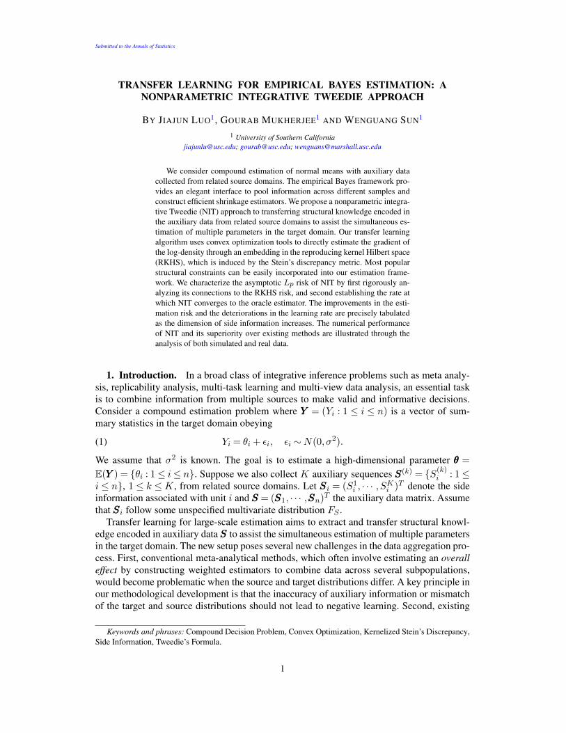
We consider compound estimation of normal means with auxiliary datacollected from related source domains. The empirical Bayes framework pro-vides an elegant interface to pool information across different samples andconstruct efficient shrinkage estimators. We propose a nonparametric integra-tive Tweedie (NIT) approach to transferring structural knowledge encoded inthe auxiliary data from related source domains to assist the simultaneous es-timation of multiple parameters in the target domain. Our transfer learningalgorithm uses convex optimization tools to directly estimate the gradient ofthe log-density through an embedding in the reproducing kernel Hilbert space(RKHS), which is induced by the Stein’s discrepancy metric. Most popularstructural constraints can be easily incorporated into our estimation frame-work. We characterize the asymptotic Lp risk of NIT by first rigorously an-alyzing its connections to the RKHS risk, and second establishing the rate atwhich NIT converges to the oracle estimator. The improvements in the esti-mation risk and the deteriorations in the learning rate are precisely tabulatedas the dimension of side information increases. The numerical performanceof NIT and its superiority over existing methods are illustrated through theanalysis of both simulated and real data.
1. Introduction. In a broad class of integrative inference problems such as meta analy-sis, replicability analysis, multi-task learning and multi-view data analysis, an essential taskis to combine information from multiple sources to make valid and informative decisions.Consider a compound estimation problem where YYY = (Yi : 1 ≤ i ≤ n) is a vector of sum-mary statistics in the target domain obeying
(1) Yi = θi + εi, εi ∼N(0, σ2).
We assume that σ2 is known. The goal is to estimate a high-dimensional parameter θθθ =
E(YYY ) = {θi : 1≤ i≤ n}. Suppose we also collect K auxiliary sequences SSS(k) = {S(k)i : 1≤
i ≤ n}, 1 ≤ k ≤K , from related source domains. Let SSSi = (S1i , · · · , SKi )T denote the side
information associated with unit i and SSS = (SSS1, · · · ,SSSn)T the auxiliary data matrix. Assumethat SSSi follow some unspecified multivariate distribution FS .
Transfer learning for large-scale estimation aims to extract and transfer structural knowl-edge encoded in auxiliary data SSS to assist the simultaneous estimation of multiple parametersin the target domain. The new setup poses several new challenges in the data aggregation pro-cess. First, conventional meta-analytical methods, which often involve estimating an overalleffect by constructing weighted estimators to combine data across several subpopulations,would become problematic when the source and target distributions differ. A key principle inour methodological development is that the inaccuracy of auxiliary information or mismatchof the target and source distributions should not lead to negative learning. Second, existing
Keywords and phrases: Compound Decision Problem, Convex Optimization, Kernelized Stein’s Discrepancy,Side Information, Tweedie’s Formula.
1
2
meta-analytical methods, which construct weighted estimators for only one or a few param-eters, can be highly inefficient in large-scale estimation problems. When thousands of pa-rameters are estimated simultaneously, useful structural knowledge, which is often encodedin auxiliary data sources, is highly informative but has been underexploited in conventionalanalyses. Finally, most transfer learning theories have focused on classification algorithms.We aim to develop a new theoretical framework to gain understandings of the benefits andcaveats of transfer learning for shrinkage estimation.
1.1. Compound decisions, structural knowledge and side information. Consider a com-pound decision problem where we make simultaneous inference of n parameters {θi : 1 ≤i≤ n} based on {Yi : 1≤ i≤ n} from n independent experiments. Let δδδ = (δi : 1≤ i≤ n) bea decision rule. Classical ideas such as the compound decision theory [32], empirical Bayes(EB) methods [33] and James-Stein shrinkage estimator [38], as well as the more recent mul-tiple testing methodologies [13, 39], showed that the joint structure of all observations ishighly informative, and can be exploited to construct more efficient classification, estimationand multiple testing procedures. For example, the submimimax rule in [32] showed that thedisparity in the proportions of positive and negative signals can be incorporated into inferenceto reduce the mis-classification rate, and the adaptive z-value procedure in [39] showed thatthe asymmetry in the shape of the alternative distribution can be utilized to construct morepowerful false discovery rate (FDR, [3]) procedures.
In light of auxiliary data, the inference units become unequal. This heterogeneity providesnew structural knowledge that can be further utilized to improve the efficiency of existingmethods. The idea is to first learn the finer structure of the high-dimensional object throughauxiliary data and then apply the new structural knowledge to the target domain. For example,in genomics research, prior data and domain knowledge may be used to define prioritizedsubset of genes. [34] proposed to up–weight the p-values in prioritized subsets where genesare more likely to be associated with the disease. Structured multiple testing is an importanttopic that has received much recent attention; see [26, 9, 27, 16, 31] for a partial list ofreferences. These works show that the power of existing FDR methods can be substantiallyimproved by utilizing auxiliary data to place differential weights or to set varied thresholdson corresponding test statistics. Similar ideas have been adopted by a few recent works onshrinkage estimation. For example, [41] and [1] propose to incorporate the side informationinto inference by first creating groups and then constructing group-wise linear shrinkage orsoft-thresholding estimators.
1.2. Nonparametric integrative Tweedie. Tweedie’s formula is an elegant and celebratedresult that has received renewed interests recently [19, 7, 12, 23, 18, 35]. Under the non-parametric empirical Bayes framework, the formula is particularly appealing for large-scaleestimation problems for it is simple to implement, removes the selection bias [12] and enjoysfrequentist’s optimality properties asymptotically [19, 7].
This article develops a nonparametric integrative Tweedie (NIT) method to extract andincorporate useful structural knowledge from both primary and auxiliary data. NIT has sev-eral merits under the transfer learning setup. First, NIT allows the target and source distri-butions to differ, which effectively avoids negative learning. Second, NIT provides a gen-eral framework for incorporating various types of structural information and can effectivelyhandle multivariate covariates. Finally, in contrast with the linear EB shrinkage estimators[42, 40, 20, 46] that are only optimal under parametric Gaussian priors, NIT belongs to theclass of generalized empirical Bayes (GEB) estimators, which enjoy asymptotic and minimaxoptimality properties for a wide class of models [45, 7].
NONPARAMETRIC INTEGRATIVE TWEEDIE 3
1.3. Main ideas of our approach. The EB implementation of Tweeide’s formula involvestwo steps: first estimating the marginal distribution and then predicting the unknown us-ing a plug-in rule. We describe some important developments in the literature. [45] showedthat a truncated GEB estimator, which is based on a Fourier infinite-order smoothing ker-nel, asymptotically achieves both the Bayes and minimax risks. The GMLEB approach by[19] implements Tweedie’s formula by estimating the unknown prior distribution via theKiefer-Wolfwitz estimator. GMLEB is approximately minimax and universally reduces theestimation risk. [7] employed a nonparametric EB estimator via Gaussian kernels and showedthat the estimator achieves asymptotic optimality for both dense and sparse means. Empiri-cally GMLEB outperforms the kernel method by [7]. However, GMLEB is computationallyintensive and may not be suitable for data–intensive applications. The connection betweencompound estimation and convex optimization was pioneered by [23], who cast GMLEBestimation as a convex program. The algorithm is fast and compares favorably to competingmethods. However, the nonparametric GEB approach to compound estimation with covari-ates has not been pursued in the literature.
We show that the EB implementation of NIT essentially boils down to the estimation ofthe log-gradient of the conditional distribution of Y given SSS. Through a carefully designedreproducing kernel Hilbert space (RKHS) representation of Stein’s discrepancy, we recastcompound estimation as a convex optimization problem, where the optimal shrinkage fac-tor is found by searching among all feasible score embeddings in the RKHS. The algorithmis computationally fast and scalable, and enjoys superior performance empirically. The ker-nelized optimization framework provides a rigorous and powerful mathematical interfacefor theoretical analysis. By appealing to the RKHS theory and concentration theories of V-statistics, we derive the approximate order of the kernel bandwidth, establish the asymptoticoptimality of the data-driven NIT procedure and explicitly characterize the impact of thedimension of covariates on the rate of convergence.
1.4. Our contributions. (1). Methodological contributions. First, NIT provides anassumption-lean framework for assimilating auxiliary data from multiple sources. Existingworks [21, 11, 24] require that the conditional mean function must be specified in the formof m(SSSi) =E(θi|SSSi) =SSSTi βββ, where βββ are regression coefficients that are usually unknown.[17] derive the minimax rates of convergence for a class of functions m(SSSi) but their workis confined to linear shrinkage estimators. By contrast, NIT does not require the specifica-tion of any functional relationship and its asymptotic optimality holds for a wider class ofprior distributions. Second, NIT is capable of incorporating various types of side informa-tion and handling multivariate covariates. By contrast, [41, 1] only focus on the variance orsparsity structure, and both methods can only handle univariate covariates. Third, NIT is fastand scalable, produces stable estimates, and provides a flexible tool for incorporating variousstructural constraints. Finally, NIT eliminates the needs for defining groups, which avoidsinformation loss in discretization as encountered in [41, 1].
(2). Theoretical contributions. First, we establish the rates at which NIT converges to theoracle integrative Tweedie estimator; this explicit characterization of the improvements in es-timation risk not only reveals how much benefits the transfer learning algorithm can provide,but also justifies the claim that NIT avoids negative learning asymptotically. Second, ourtheory precisely tabulates the deteriorations in the learning rates as the dimension of side in-formation increases. This gives caveats on utilizing high-dimensional auxiliary data. Finally,we develop new analytical tools to formalize the theoretical properties of the optimizationframework using kernelized Stein’s discrepancy (KSD). The KSD approach has been appliedin a host of recent statistical and machine learning problems [28, 10, 43, 29, 30, 2]. The suc-cess of KSD based methods critically depends on the conjecture that a lower risk in RKHS
4
norm would translate to a lower Lp risk. However, a general isometry theory between theRKHS and Lp risks does not exist. Our work provides the first rigorous analysis that estab-lishes this isometry (in the context of compound estimation); the probability tools therein canbe of independent interest for decision theorists.
1.5. Organization of the Paper. The article is organized as follows. In Section 2, wediscuss the empirical Bayes estimation framework, NIT estimator and computational algo-rithms. Section 3 studies the theoretical properties of the NIT estimator. Sections 4 and 5investigate the performance of NIT using simulated and real data respectively. We concludethe article with a discussion of some open problems. Additional technical details and proofsare provided in the Supplementary Material.
2. Methodology. Let δδδ(yyy,sss) = (δi : 1 ≤ i ≤ n) be an estimator of θθθ and L2n(δδδ,θθθ) =
n−1∑n
i=1(θi − δi)2 the loss function. Define the risk Rn(δδδ,θθθ) = EYYY ,SSS|θθθ{L2n(δδδ,θθθ)
}and the
Bayes risk Bn(δδδ) =∫Rn(δδδ,θθθ)dΠ(θθθ), where Π(θθθ) is an unspecified prior.
The transfer learning setup may be conceptualized via a hierarchical model. We assumethat the primary and auxiliary data are related through a latent vector ξξξ = (ξ1, · · · , ξn)T :
(2)θi = gθ(ξi, ηy,i), 1≤ i≤ n,
s(j)i = gsj (ξi, ηj,i), 1≤ j ≤K,
where gθ and gsj are unspecified functions, and ηy,i and ηj,i are random perturbations thatare independent from ξξξ. This hierarchical model provides a general framework that can beutilized to incorporate both continuous and discrete auxiliary data into inference.
This section first introduces an oracle rule that optimally borrows information from SSS,then discusses a data-driven rule that emulates the oracle rule.
2.1. Learning via integrative Tweedie. Consider an oracle with access to the joint densityf(y|sss). We study the optimal rule that minimizes the Bayes risk. The integrative Tweedie’sformula, given by the next proposition, generalizes Tweedie’s formula ([33, 12]) from theclassical setup to the transfer learning setup.
PROPOSITION 1 (Integrative Tweedie). Consider the hierarchical model (1) and (2). Letf(y|sss) be the conditional density of Y given SSS. The optimal estimator that minimizes theBayes risk is δδδπ(yyy,sss) = {δπ(yi,sssi) : 1≤ i≤ n}, where
(3) δπ(y,sss) = y+ σ2∇y log f(y|sss).
Integrative Tweedie is simple and intuitive, nonetheless it provides a general and flexibleframework for transfer learning. First, existing works on shrinkage estimation with side in-formation require that the form of the conditional mean function m(SSSi) = E(Yi|SSSi) mustbe pre-specified [21, 11, 24]. By contrast, integrative Tweedie incorporates the side infor-mation via a general function f(y|sss), which eliminates the need to pre-specify a fixed rela-tionship between Y and SSS. Next, the effectiveness of existing transfer learning algorithmscritically depends on the similarity between the target and source distributions, and maysuffer from negative learning when the target and source distributions differ. By contrast, in-tegrative Tweedie effectively avoids negative learning; the auxiliary data SSS are only utilizedthrough f(y|sss) to assist inference by providing the structural knowledge of Y .
To illustrate the key advantages of the new transfer learning machinery, we present twotoy examples, which respectively show that: (a) If the two distributions match perfectly, thenintegrative Tweedie reduces to an intuitive data averaging strategy; (b) If the two distributionsdiffer, then integrative Tweedie is still effective in reducing the risk.

NONPARAMETRIC INTEGRATIVE TWEEDIE 5
EXAMPLE 1. Suppose (Yi, Si) are conditionally independent given (µi,y, µi,s). We beginby considering a case where Si is an independent copy of Yi:
µi ∼N(µ0, τ2), Yi = µi + εi, Si = µi + ε′i,
where εi ∼N(0, σ2), ε′i ∼N(0, σ2). Intuitively, the optimal Bayes estimator is to use Zi =(Yi + Si)/2∼N(µi, σ
2/2) as the new data point:
(4) µopi =12σ
2µ0 + τ2Zi12σ
2 + τ2=σ2µ0 + τ2(Yi + Si)
σ2 + 2τ2.
For this bivariate normal model, the conditional distribution of Yi given Si is Yi|Si ∼N(σ2µ0 + τ2Si/(τ
2 + σ2), σ2(2τ2 + σ2)/(τ2 + σ2)). It follows that l′(Yi|Si) = σ−2(2τ2 +
σ2)−1(τ2Si + σ2µ0)− Yi(τ2 + σ2).We obtain δπi = (σ2 +2τ2)−1{σ2µ0 +τ2(Yi+Si)}, re-covering the optimal estimator (4). It is important to note that if we slightly alter the model,say perturbating Si by ηi: Si = µi + ηi + ε′i, or letting Si = f(µi) + ε′i, then averaging Y andS via (4) may lead to negative learning. However, integrative Tweedie provides a robust datacombination approach that always leads to a reduction in estimation risk (Proposition 2).
EXAMPLE 2. Suppose that Si is a group indicator. The two groups (S = 1 and S = 2)have equal sample sizes. The primary data obey Yi|Si = k ∼ (1− πk)N(0,1) + πkN(µi,1),with π1 = 0.01, π2 = 0.4 and µi ∼N(2,1). Consider two oracle Bayes rules δπi (Yi, Si) andδπi (Yi). Some calculations yield[
B(δπi (Yi))−B{δπi (Yi, Si)}]/B{δπi (Yi)}= 0.216,
which shows that incorporating Si can reduce the risk by as much as 21.6%. It is importantto note that the distributions of Yi and Si are very different (continuous vs. binary), makingit difficult for conventional machine learning algorithms to pool information across the targetand source domains. Integrative Tweedie is still highly effective in reducing estimation riskby exploiting the grouping structure encoded in Si.
2.2. Nonparametric estimation via convex programming. This section develops a data-driven procedure to emulate the oracle rule. Denote the collection of all data by X =(xxx1, · · · ,xxxn)T , where for i= 1, . . . , n, we have x1i = yi and the summary statistics collectedfrom the kth source domain constitute xki = s
(k−1)i for k = 2, . . . ,K + 1. Our goal is to
estimate the shrinkage factor
hhhf (XXX) =
{∇u1
log f(u1|u2, . . . , uK+1)∣∣uuu=xxxi
: 1≤ i≤ n}
= {∇yi log f(yi|sssi) : 1≤ i≤ n}.
Let Kλ(xxx,xxx′) be a kernel function that is integrally strictly positive definite; λ is a tuningparameter. A detailed discussion on the construction of kernel K(·, ·) and choice of λ isprovided in Section 2.3. Consider the following two n× n matrices:
(KKKλ)ij = n−2Kλ(xxxi,xxxj), (∇KKKλ)ij = n−2∇x1jKλ(xxxi,xxxj) .
For a fixed λ, let hhhλ,n be the solution to the following quadratic program:
(5) arg minhhh∈VVV n
hhhTKKKλhhh+ 2hhhT∇KKKλ111,
where VVV n is a convex subset of Rn. We give two remarks.
REMARK 1. Convex constraints such as linearity and monotonicity, detailed in Section2.3, are fundamental to the compound decision problem [23]. The constraints imposed viaVVV n can improve the stability and efficiency of the shrinkage estimator.
6
REMARK 2. The convex program (5) is motivated by the kernelized Stein’s discrepancy(KSD; [28, 10, 2]), a useful tool in our theoretical analysis formally defined in Section 3.Roughly speaking, the KSD measures how far a given hhh is from the true score hhhf . The KSDis always non-negative, and is equal to 0 if and only if hhh = hhhf . Hence, solving the convexprogram (5) is equivalent to finding a shrinkage estimator (assisted by side information) thatmakes the estimation risk as small as possible.
Proposition 1 motivates us to consider the following class of nonparametric integrativeTweedie (NIT) estimators{
δδδITλ : λ ∈ (0,∞)
}, where δδδ
ITλ = yyy+ σ2
y hhhλ,n.(6)
In Section 3, we show that as n→∞ there exist choices of λ such that hhhλ,n can estimate hhhfwith negligible errors. It follows that the resulting estimator (6) is asymptotically optimal
The NIT estimator (6) marks a clear departure from existing GMLEB methods [19, 23, 15],which cannot be easily extended to handle multivariate auxiliary data. Moreover, NIT hasseveral additional advantages over existing nonparametric GEB methods in both theory andcomputation. First, in comparison with the GMLEB method [19], the convex program (5) isfast and scalable. Second, [7] proposed to estimate the score function by the ratio f (1)/f ,where f is a kernel density estimate and f (1) is its derivative. By contrast, our direct opti-mization approach avoids computing ratios and produces more stable and accurate estimates.Third, our convex program can be fine-tuned by selecting a suitable λ. This leads to improvednumerical performance and enables a disciplined theoretical analysis compared to the pro-posal in [23]. Finally, the criterion in (5) can be rigorously analyzed to establish new rates oftransfer learning (Sec. 3.1) that are unknown in the literature.
2.3. Computational details. This section provides the following details in computation:(a) how to impose convex constraints; (b) how to construct kernel functions to handle multi-variate and possibly correlated covariates; and (c) how to choose the bandwidth λ.
1. Structural constraints. We illustrate how to design appropriate constraints to enforceunbiasedness and monotonicity conditions. The unbiasedness can be achieved by setting∑n
i=1 hi = 0, with corresponding linear constraints given by 111Thhh = 0. The monotonic-ity constraints proposed in [23] are highly effective for improving the estimation accu-racy. These constraints can be included as Mhhh � aaa. For ease of presentation, assume thaty1 ≤ y2 ≤ · · · ≤ yn. To impose the monotonicty constraints σ2hi−1−σ2hi ≤ yi−yi−1 for alli, we chooseM as the following upper triangular matrixMij = σ2(I{i= j}−I{i= j−1}),and let aaaT = (y2 − y1, y3 − y2, · · · , yn − yn−1).
2. Kernel functions. The kernel function needs to be carefully constructed to dealwith various complications in the multivariate setting, where the auxiliary sequences SSSk,1≤ k ≤M , may be correlated and have different measurement units. We propose to use the
Mahalanobis distance ‖xxx− xxx′‖Σxxx=√
(xxx−xxx′)TΣ−1xxx (xxx−xxx′) in the kernel function, where
Σxxx is the sample covariance matrix. The RBF kernel isKλ(xxx,xxx′) = exp{−0.5λ2‖xxx−xxx′‖2Σxxx},
where λ is the bandwidth whose choice is discussed next. Compared to the Euclidean dis-tance that treats each coordinate equally, Mahalanobis distance is more suitable for combin-ing data collected from heterogeneous sources for it is unitless, scale-invariant and takes intoaccount the correlation in the data. When auxiliary data contain both continuous and categor-ical variables, we propose to use the generalized Mahalanobis distance [25]. We illustrate themethodology for mixed types of variables in the numerical studies in Section 4.1 (Setting 4),but only pursue theory for the case where both YYY and SSS are continuous.
NONPARAMETRIC INTEGRATIVE TWEEDIE 7
3. Modified cross-validation (MCV). Implementing the NIT estimator requires selectingthe tuning parameters λ. Following [8], we propose to determine λ via modified cross val-idation (MCV). Let ηi ∼N (0, σ2), 1≤ i≤ n be i.i.d. noise variables independent of yyy andsss1, · · · ,sssK . Define Ui = yi + αηi and Vi = yi − ηi/α. Then, Ui and Vi are independent. TheMCV uses UUU = {U1, · · · ,Un} for constructing estimators δITλ (UUU,SSS), while using V1, · · · , Vnfor validation. Consider the validation loss
Ln(λ,α) =1
n
n∑i=1
{δITλ,i(UUU,SSS)− Vi
}2 − σ2(1 + 1/α2) .
For a small α, the data-driven bandwidth is chosen by minimizing Ln(λ,α), i.e., λ =
arg minλ∈Λ Ln(λ,α) for any Λ ⊂ R+ and the proposed NIT estimator is {yi + σ2yhhhλ,n(i) :
1≤ i≤ n}. Proposition 3 in Section 3.6 shows that asymptotically the validation loss is closeto the true loss, justifying the aforementioned algorithm.
3. Theory. This section develops large-sample theory for the data-driven NIT estimator.We assume that XXXi = (Yi, Si1, · · · , Sik)T , i = 1, · · · , n, are i.i.d. samples from a continu-ous multivariate density f on RK+1. Denote X = (XXX1, · · · ,XXXn)T the n× (K + 1) matrixof observations and XXX(k) be the kth column of X. Let f be a density function defined onRK+1 and hf (xxx) = ∇1 log f(x1|xxx−1) the conditional score function corresponding to thefirst coordinate, where xxx−1 = {xj : 2 ≤ j ≤K + 1}. It follows from the definition that thisconditional score is same as the log-gradient of the joint density for the first coordinate,i.e., hf (xxx) =∇1 log f(xxx). Recall that we aim to estimate θθθ = E
{XXX(1)
}. The score function
hf (xxx), by Proposition 1, plays the key role in the oracle NIT estimator. We next show howhf (xxx) can be well estimated by the solution to (5).
3.1. Kernelized Stein’s discrepancy. We first introduce the kernelized Stein’s discrep-ancy. Consider the Gaussian kernel function Kλ : RK+1 × RK+1 → R with bandwidth λ.Let P andQ denote two conditional univariate distributions (conditional on aK-dimensionalcovariate) on RK+1. Denote p and q the respective conditional densities and hp and hq thescore functions. The kernelized Stein’s discripancy (KSD; [28, 10, 2]) between P and Q isthe kernel weighted distance between hp and hq:
Dλ(P,Q) = E(uuu,vvv)
i.i.d.∼ P{Kλ(uuu,vvv)× (hp(uuu)− hq(uuu))× (hp(vvv)− hq(vvv))} .
The KSD is closely connected to the maximum mean discrepancy (MMD, [14]). MinimizingKSD is a popular technique in several satistical applications. It has been recently appliedto the development of new goodness-of-fit tests [28, 10, 43], bayesian inference procedures[29, 30] and simultaneous estimation methods [2]. Compared to the MMD, the KSD is par-ticularly suitable for empirical Bayes estimation because it can be directly constructed basedon the score functions, which by Proposition 1 yield the optimal shrinkage factors. It can beshown that the KSD satisfies
Dλ(P,Q)≥ 0 and Dλ(P,Q) = 0 if and only if P =Q.
The direct evaluation of Dλ(P,Q) is difficult. Next we discuss an alternative represen-tation of the KSD that can be easily evaluated empirically. Specifically, for any functionalh : RK+1→R, define the following quadratic functional κλ[h] over RK+1 ×RK+1:
κλ[h](uuu,vvv) =Kλ(uuu,vvv)h(uuu)h(vvv) +∇vvvKλ(uuu,vvv)h(uuu) +∇uuuKλ(uuu,vvv)h(vvv) +∇uuu,vvvKλ(uuu,vvv) .(7)
The alternative representation of the KSD, given in [28, 10], uses the quadratic function in(7) and only involves the score function of q:
(8) Dλ(P,Q) = E(uuu,vvv)
i.i.d.∼ P{κλ[hq](uuu,vvv)}.
8
Now we turn to the compound estimation problem and discuss its connection to the KSD.Proposition 1 shows that, when f is known, the optimal estimator is constructed based onhhhf (XXX) = {hf (xxx1), . . . ,hf (xxxn)}T , the conditional score function evaluated at the n observeddata points. Define
Sλ,n(hhh) =hhhTKKKλhhh+ 2hhhT∇KKKλ111 + 111T∇2KKKλ111,(9)
where (∇2KKKλ)ij = n−2∇x1j∇x1i
Kλ(xxxi,xxxj), KKKλ is the n× n Gaussian kernel matrix withthe bandwith λ and ∇KKKλ is defined in Section 2.2. It is easy to see that the convexprogram (5) is equivalent to minimizing Sλ,n(hhh) over hhh1. Now, note that when hhh equalshhhq = {hq(xxx1), . . . ,hq(xxxn)}, (9) is just the empirical version of the KSD defined in (8):
Sλ,n(hhhq) =Dλ(Fn,Q) = E(uuu,vvv)
i.i.d.∼ Fn
{κλ[hq](uuu,vvv)}=1
n2
n∑i,j=1
κλ[hq](xxxi,xxxj) ,
where Fn is the empirical distribution function.We are now ready to explain the heuristic idea behind the optimization criterion (5).
As n → ∞, Fn → F and one can show that Sλ,n(hhhq) → Sλ(hq) := Dλ(F,Q). More-over, Dλ(F,Q) = 0 iff F = Q. Thus, if we could have minimized Sλ(hq) over the classH = {hq =∇1 log q(xxx) : q is any density on RK+1}2, then the minimum would be achievedat the true score function hf and the minimum value would be 0. However, Sλ(hq) involvesthe unknown true distribution F , which makes such a direct minimization impossible. Alter-natively, we minimize the corresponding sample based criterion Sλ,n(hhhq) in (9) (or equiva-lently, (5)). In large-sample situations, we expect the sampling fluctuations to be small; hence,minimizing Sλ,n will lead to score function estimates very close to the true score functions.The convergence rates of the estimates are established next.
3.2. Score estimation under the Lp loss. The next two subsections formulate a rigoroustheoretical framework, in the context of compound estimation, to derive the convergence ratesof the proposed estimator.
The criterion (5) involves minimizing the V-statistic Sλ,n(hhh). Using standard asymptoticsresults for V-statistics [37], it follows that for any density q, Sλ,n(hhhq)→Sλ(hq) in probabilityas n→∞. Also, it follows that hhhλ,n, the solution to (5), satisfies:
n−2∑i,j
Kλ(xxxi,xxxj){hhhλ,n(i)− hf (xxxi)
} {hhhλ,n(j)− hf (xxxj)
}=OP (n−1)(10)
as n→∞ , where hhhλ,n(i) = hhhλ,n(xxxi) for i= 1, . . . , n.While (10) shows that in the RKHS norm the estimates are asymptotically close to the
true score functions, for most practical purposes we need to establish the convergence underthe `p norm. For p > 0, define `p(hhhλ,n,hf ) = n−1
∑ni=1 |hhhλ,n(xixixi) − hf (xxxi)|p. The case of
p= 2 corresponds to Fisher’s divergence. Denote the RKHS norm on the left side of (10) bydλ(hhhλ,n,hf ). The essential difficulty in the analysis is that the isometry between the RKHSmetric and `p metric may not exist. Concretely, for any λ > 0, we can show that dλ ≤C1 `2,where C1 is a constant. However, the inequality in the other direction does not always hold.
1This can be easily seen because the extra term 111T∇2KKKλ111 does not involve hhh.2For implementational ease, we relax the optimization space from the set of all conditional score functionsH
to the set all of all real functionals on RK+1. Due to the presence of structural constraints discussed in Section2.1, this relaxation has little impact on the numerical performance of the NIT estimator. Simulations in Section 4show that the solutions to (5) produce efficient estimates.
NONPARAMETRIC INTEGRATIVE TWEEDIE 9
We aim to show that `2 ≤C2 dλ for some constant C2; this would produce the desired boundon the Lp risk. Next we provide an overview of the main ideas and key contributions of thetheoretical analyses in later subsections.
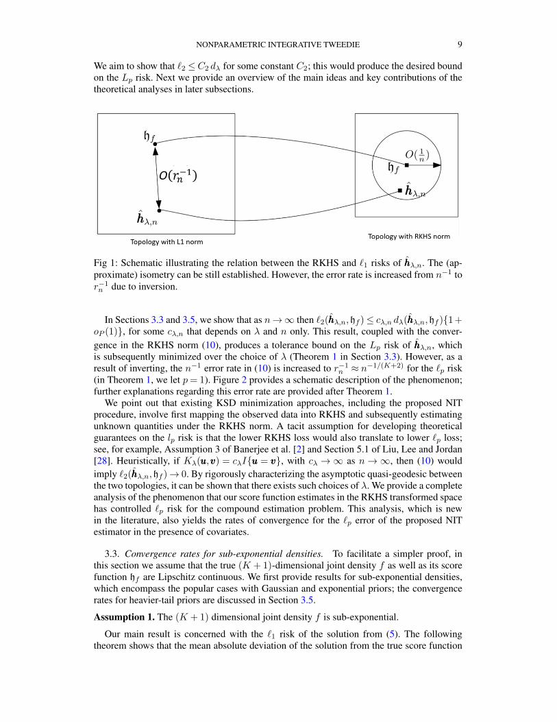
Fig 1: Schematic illustrating the relation between the RKHS and `1 risks of hhhλ,n. The (ap-proximate) isometry can be still established. However, the error rate is increased from n−1 tor−1n due to inversion.
In Sections 3.3 and 3.5, we show that as n→∞ then `2(hhhλ,n,hf )≤ cλ,n dλ(hhhλ,n,hf ){1 +oP (1)}, for some cλ,n that depends on λ and n only. This result, coupled with the conver-gence in the RKHS norm (10), produces a tolerance bound on the Lp risk of hhhλ,n, whichis subsequently minimized over the choice of λ (Theorem 1 in Section 3.3). However, as aresult of inverting, the n−1 error rate in (10) is increased to r−1
n ≈ n−1/(K+2) for the `p risk(in Theorem 1, we let p= 1). Figure 2 provides a schematic description of the phenomenon;further explanations regarding this error rate are provided after Theorem 1.
We point out that existing KSD minimization approaches, including the proposed NITprocedure, involve first mapping the observed data into RKHS and subsequently estimatingunknown quantities under the RKHS norm. A tacit assumption for developing theoreticalguarantees on the lp risk is that the lower RKHS loss would also translate to lower `p loss;see, for example, Assumption 3 of Banerjee et al. [2] and Section 5.1 of Liu, Lee and Jordan[28]. Heuristically, if Kλ(uuu,vvv) = cλI{uuu = vvv}, with cλ →∞ as n→∞, then (10) wouldimply `2(hhhλ,n,hf )→ 0. By rigorously characterizing the asymptotic quasi-geodesic betweenthe two topologies, it can be shown that there exists such choices of λ. We provide a completeanalysis of the phenomenon that our score function estimates in the RKHS transformed spacehas controlled `p risk for the compound estimation problem. This analysis, which is newin the literature, also yields the rates of convergence for the `p error of the proposed NITestimator in the presence of covariates.
3.3. Convergence rates for sub-exponential densities. To facilitate a simpler proof, inthis section we assume that the true (K + 1)-dimensional joint density f as well as its scorefunction hf are Lipschitz continuous. We first provide results for sub-exponential densities,which encompass the popular cases with Gaussian and exponential priors; the convergencerates for heavier-tail priors are discussed in Section 3.5.
Assumption 1. The (K + 1) dimensional joint density f is sub-exponential.
Our main result is concerned with the `1 risk of the solution from (5). The followingtheorem shows that the mean absolute deviation of the solution from the true score function
10
is asymptotically negligible as n→∞. In the theorem we adopt the notation an � bn for twosequences an and bn, which means that c1an ≤ bn ≤ c2bn for all large n and some constantsc2 ≥ c1 > 0.
THEOREM 1. Under assumption 1, as n→∞ with λ� n−1/(K+2),
rn ·(
1
n
n∑i=1
|hhhλ,n(i)− hf (xxxi)|)→ 0 in L1,(11)
where, rn = n1/(K+2)(log(n))−(2K+5).
REMARK 3. It follows immediately from Theorem 1 that the deviations between ourproposed estimate and the oracle estimator in (3) obeys:
rn
(1
n
n∑i=1
∣∣∣δδδITλ (i)− δπi (yi|sssi)∣∣∣)→ 0 in L1 as n→∞.(12)
Under the classical setting with no auxiliary data (K = 0), we achieve the traditional√n−rate as established in Jiang and Zhang [19]. In this context, the rates are sharp.
We can see that, barring the poly-log terms, the convergence rate rn = n1/(K+2) decreasesas K increases. We provide further discussions on this attribute, as well as its implicationsfor transfer learning, in Section 3.4.
Next we sketch the outline of and main ideas behind the proof of Theorem 1; detailedarguments are provided in the supplement. Consider
∆λ,n := E{dλ(hhhλ,n,hf )}= EXXXn
[Kλ(xxx1,xxxn)
{hhhλ,n(1)− hf (xxx1)
} {hhhλ,n(n)− hf (xxxn)
}],
where the expectation is taken overXXXn = {xxx1, . . . ,xxxn} andxxxi are i.i.d. samples from f . From(10) it follows that ∆λ,n = O(n−1). For λ→ 0, Kλ(xxx1,xxxn) is negligible only when ||xxx1 −xxxn||2 is small. Thus for studying the asymptotic behavior of ∆λ,n, we shall restrict ourselveson the event where ||xxx1 − xxxn||2 is small. Conditional on this event, we show that ∆λ,n canbe well approximated by κλ,n∆λ,n−1, where ∆λ,n−1 = EXXXn−1
{(hhhλ,n(1)− hf (xxx1))2f(xxx1)}and the expectation is taken over XXXn−1 = {xxx1, . . . ,xxxn−1}. To heuristically understand thegenesis of ∆λ,n−1, substitute xxx1 + εεε in place of xxxn in the expression:
∆λ,n =
∫Kλ(xxx1,xxxn)(hhhλ,n(1)− hf (xxx1))
(hhhλ,n(n)− hf (xxxn)
)f(xxx1) . . . f(xxxn)dxxx1 . . . dxxxn
and let |εεε| → 0. As λ→ 0, the contributions from the kernel weight Kλ can be separated outof the expression and subsequently accounted by constants κλ,n. Meanwhile the remainingterms produce ∆λ,n−1. The rate at which |εεε| → 0 needs to be appropriately tuned with λto get the optimal rate of convergence; a rigorous probability argument is provided in thesupplement. We shall see that the intermediate quantity ∆λ,n−1, which links the Lp andRKHS norms, can be explicitly characterized. The rate of convergences will be establishedby sandwiching ∆λ,n−1 with functionals involving L1 and L2 norms.
Finally we present a result investigating the performance of the NIT estimator under themean squared loss. Using sub-exponential tail bounds, the `2 loss of score functions can beobtained by extending the results on `1 loss. The difference in the mean squared losses be-tween the oracle and data-driven NIT estimators can be subsequently characterized. Lemma 2below shows that this difference is asymptotically negligible.
NONPARAMETRIC INTEGRATIVE TWEEDIE 11
LEMMA 2. For any unknown prior π satisfying assumption 1 and λ� n−1/(K+2),
L2n(δδδ
IT
λ ,θθθ)−L2n(δδδπ,θθθ) = op(r
−1n ) as n→∞.(13)
Combining (12) and (13), we have established the asymptotic optimality of the data-drivenNIT procedure by showing that it achieves the risk performance of the oracle rule asymptot-ically when n→∞; this theory is corroborated by the numerical studies in Section 4.
3.4. Benefits and caveats in exploiting auxiliary data. The amount of efficiency gain ofthe data-driven NIT estimator depends on two factors: (a) the usefulness of the side informa-tion and (b) the precision of the approximation to the oracle. Intuitively when the dimensionof the side information increases, the former increases whereas the latter deteriorates.
Consider the Tweedie estimator yi +σ2∇ log f1(yi) that only uses the marginal density f1
of Y and no auxiliary information. The Fisher information based on the marginal f1 and theconditional density f(y|sss) are
IY =
∫ {f ′1(y)
f1(y)
}2
f1(y)dy and IY |SSS =
∫ {∇yf(y|sss)f(y|sss)
}2
f(y,sss)dy dsss .
The following proposition, which follows from Brown [6] (for completeness a proof is pro-vided in the supplement), shows that, under the oracle setting, utilizing side information isalways beneficial, and the efficiency gain becomes larger when more columns of auxiliarydata are incorporated into the estimator.
PROPOSITION 2. Consider hierarchical model (1)–(2). Let δδδπ(yyy) and δδδπ(yyy,SSS) respec-tively denote the oracle estimator with only yyy and the oracle estimator with both yyy and SSS.The efficiency gain due to usage of auxiliary information is
Bn {δδδπ(yyy)} −Bn {δδδπ(yyy,SSS)}= σ4y
(I(Y |SSS) − IY
)≥ 0 .
The above equality is attained if and only if the primary variable is independent of all auxil-iary variables.
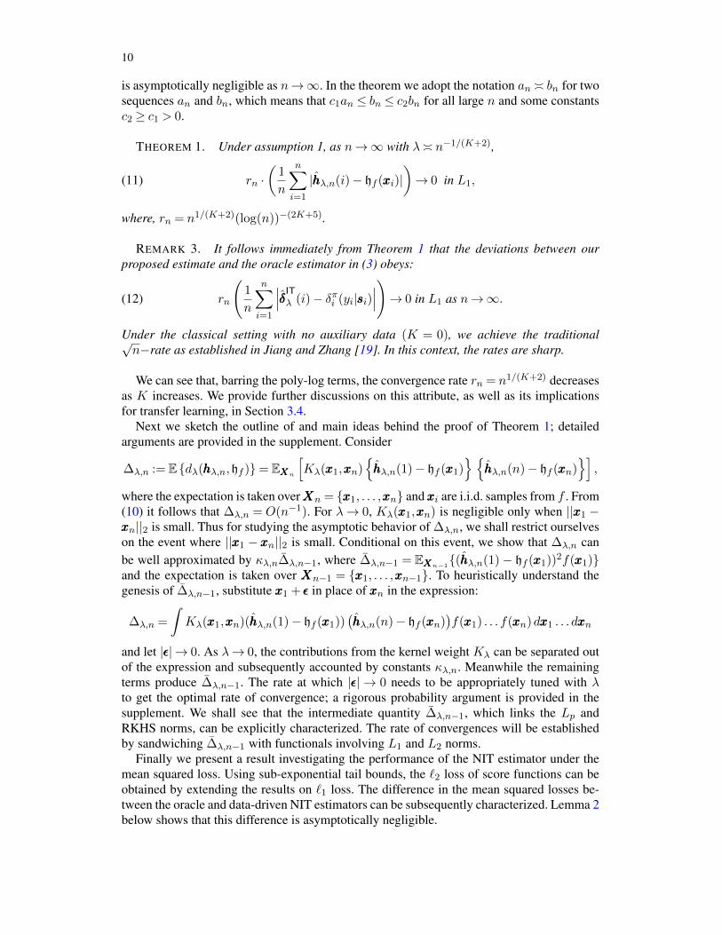
In Theorem 1 and Lemma 2, the rate of convergence rn decreases as K increases. Inlight of Proposition 2, this means that although theoretically we never lose by adding morecolumns of auxiliary data (even if they are non-informative), there is still a tradeoff underour estimation framework. The increase of K leads to a widened gap between the oracle anddata-driven rules, which may offset the benefits of incorporating more side information. Thefollowing numerical example illustrates two aspects of the phenomenon.
Consider the hierarchical model (1)–(2). We draw the latent vector ξξξ from a two-pointmixture model, with equal probabilities on two atoms 0 and 2, i.e. ξi ∼ 0.5δ{0} + 0.5δ{2}.The mean vectors are simulated as θi = ξi + ηy,i and µk,i = ξi + ηk,i, 1 ≤ k ≤ K with
ηy,i, ηk,ii.i.d.∼ N (0,1). Finally we generate Yi ∼N (θi,1) and Sk,i ∼N (µk,i,1), 1≤ k ≤K .
We vary K from 1 to 12 and compare the oracle and data-driven NIT procedures in Figure2. We can see that the increase of K has two effects: (a) the MSE of the oracle NIT proce-dure decreases steadily, while (b) the gap between the oracle and data-driven NIT proceduresincreases quickly. The combined effect initially leads to a rapid decrease in the MSE of thedata-driven NIT procedure, but the decline slackens as K ≥ 5.
12
Fig 2: Mean squared error of our proposed method (in magenta) is plotted along with theoracle risk (in sky blue) as the number of auxiliary variable (K) increases. The MSE ofthe oracle procedure always decreases but the MSE of the data-driven NIT procedure stopsdecreasing as K ≥ 9.
3.5. Convergence rates for heavy-tail densities. We extend the results in Section 3.3to a wider class of prior distributions. To rule out cases where ||hf ||2 is negligible (such asuniform prior), we consider the following mild assumption on the prior that rules out densitieswith tail behaviors heavier than Cauchy.
Assumption 2: The class of priors π(θ) satisfy: θ2π(θ) is bounded for all θ.
The next theorem shows that, for suitably chosen bandwidth, the data-driven NIT estimator isasymptotically close to the oracle estimator and the difference in their losses also convergesto 0 under any prior satisfying Assumption 2. The rate of convergence is slower than that ofTheorem 1, which is mainly due to the larger terms needed to bound heavier tails. Similar toTheorem 1, the rate decreases with the increase of K .
THEOREM 3. Under Assumption 2, with λ� n−1/(K+2) and rn = n1/(3(K+2)), we have
rn ·(
1
n
n∑i=1
|hhhλ,n(i)− hf (xxxi)|)→ 0 in L1 as n→∞.
Additionally, we have L2n(δδδ
IT
λ ,θθθ)−L2n(δδδπ,θθθ) = op(r
−1n ) as n→∞.
3.6. Consistency of the MCV criterion. In Sections 3.3 and 3.5, we have establishedasymptotic risk proporties of our proposed method as bandwidth λ→ 0. For finite samplesizes, it is important to select the “best” bandwidth based on a data-driven criterion as pro-vided in Section 2.3. The following proposition establishes the consistency of the validationloss to the true loss, justifying the effectiveness of the bandwidth selection rule.
NONPARAMETRIC INTEGRATIVE TWEEDIE 13
PROPOSITION 3. For any fixed λ > 0 and n, we have
limα→0
E{Ln(λ,α)−L2
n(δδδIT
λ ,θθθ)}
= 0 .
provided that there is a unique solution to (5) for α= 0.
4. Simulation. We consider three different settings where the structural information isencoded in (a) one given auxiliary sequence that shares structural information with the pri-mary sequence through a common latent vector (Section 4.1); (b) one auxiliary sequencecarefully constructed within the same data to capture the sparsity structure of the primary se-quence (Section 4.2); (c) multiple auxiliary sequences that share a common structure with theprimary sequence (Section 4.3). We conduct simulations to compare the following methods:
• James-Stein estimator (JS).• The empirical Bayes Tweedie (EBT) estimator implemented using kernel smoothing as
described in [7].• Non-parametric maximum likelihood estimator (NPMLE), which implements Tweedie’s
formula using the convex optimization approach [23]. The method is implemented by theR-package “REBayes” in [22].
• Empirical Bayes with cross-fitting (EBCF) by [17].• The oracle NIT procedure (3) with known f(y|sss) (NIT.OR).• The data-driven NIT procedure (6) by solving the convex program (NIT.DD).
The last three methods, which utilize auxiliary data, are expected to outperform the first threemethods when the side information is informative. The MSE of OR is provided as the optimalbenchmark for assessing the efficiency of various methods.
In the implementation of NIT.DD, we utilize the generalized Mahalanobis distance, dis-cussed in Section 2.3, to compute the RBF kernel with bandwidth λ. A data-driven choiceof the tuning parameter λ is obtained by first solving optimization problems 5 over a grid ofλ values and then computing the corresponding modified cross-validation (MCV) loss. Wechoose the λ with minimum MCV loss as the data-driven bandwidth.
4.1. Simulation 1: integrative estimation with one auxiliary sequence. Let ξξξ = (ξi : 1≤i≤ n) be a latent vector obeying a two-point normal mixture:
ξi ∼ 0.5N (0,1) + 0.5N (1,1).
The primary data YYY = (Yi : 1 ≤ i ≤ n) in the target domain are simulated according to thefollowing hierarchical model:
θi ∼N (ξi, σ2), Yi ∼N (θi,1).
By contrast, the auxiliary data SSS = (Si : 1≤ i≤ n) obeys
ζi ∼N (ξi, σ2), Si ∼N (ζi, σ
2s).
The above data generating mechanism is a special case of the hierarchical model (2). Both theprimary parameter θi and auxiliary parameter ζi are related to a common latent variable ξi,with σ controlling the amount of common information shared by θi and ζi. We further use σsto reflect the noise level when collecting data in the source domain. The auxiliary sequenceSSS becomes more useful when both σ and σs decrease. We consider the following settings toinvestigate the impact of σ, σs and sample size n on the performance of different methods.
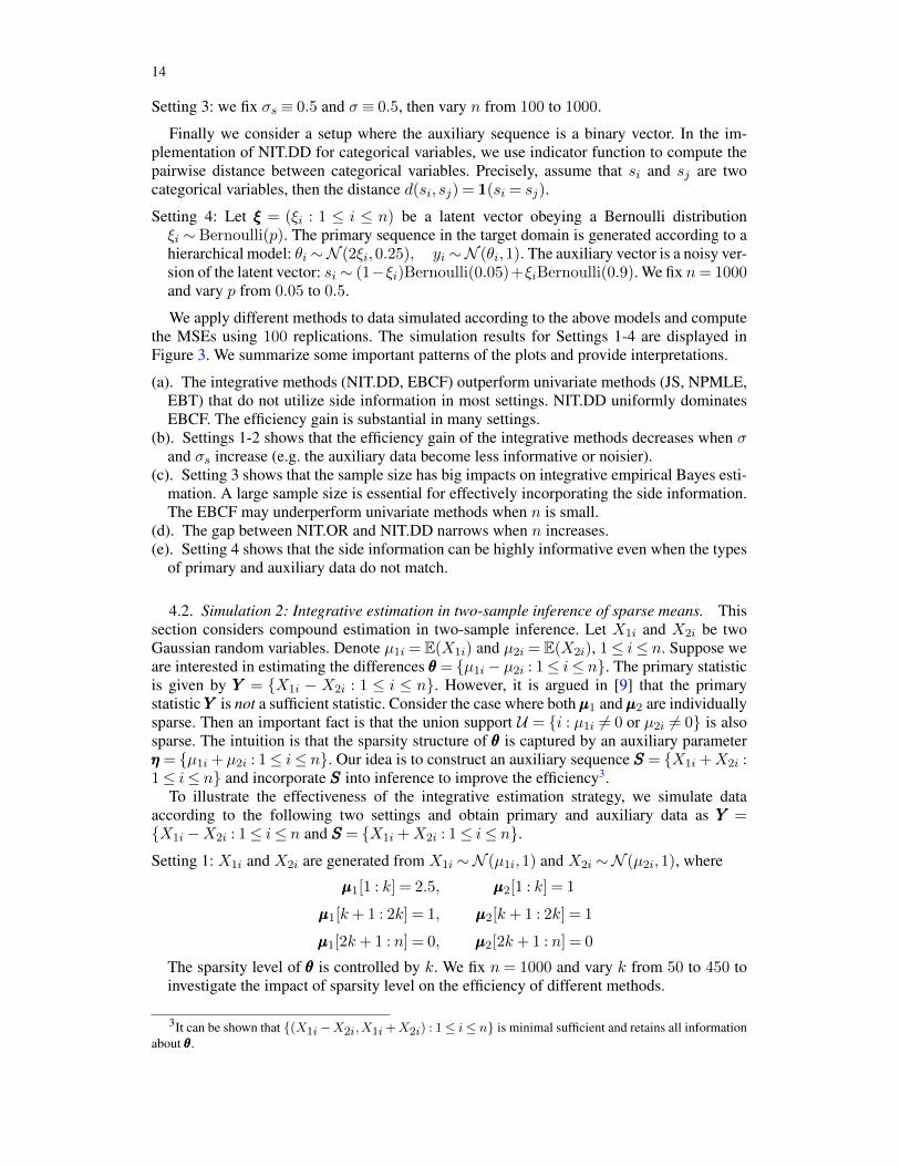
Setting 1: we fix n= 1000 and σ ≡ 0.1, then vary σs from 0.1 to 1.Setting 2: we fix n= 1000 and σs ≡ 1, then vary σ from 0.1 to 1.
14
Setting 3: we fix σs ≡ 0.5 and σ ≡ 0.5, then vary n from 100 to 1000.
Finally we consider a setup where the auxiliary sequence is a binary vector. In the im-plementation of NIT.DD for categorical variables, we use indicator function to compute thepairwise distance between categorical variables. Precisely, assume that si and sj are twocategorical variables, then the distance d(si, sj) = 1(si = sj).
Setting 4: Let ξξξ = (ξi : 1 ≤ i ≤ n) be a latent vector obeying a Bernoulli distributionξi ∼ Bernoulli(p). The primary sequence in the target domain is generated according to ahierarchical model: θi ∼N (2ξi,0.25), yi ∼N (θi,1). The auxiliary vector is a noisy ver-sion of the latent vector: si ∼ (1−ξi)Bernoulli(0.05)+ξiBernoulli(0.9). We fix n= 1000and vary p from 0.05 to 0.5.
We apply different methods to data simulated according to the above models and computethe MSEs using 100 replications. The simulation results for Settings 1-4 are displayed inFigure 3. We summarize some important patterns of the plots and provide interpretations.
(a). The integrative methods (NIT.DD, EBCF) outperform univariate methods (JS, NPMLE,EBT) that do not utilize side information in most settings. NIT.DD uniformly dominatesEBCF. The efficiency gain is substantial in many settings.
(b). Settings 1-2 shows that the efficiency gain of the integrative methods decreases when σand σs increase (e.g. the auxiliary data become less informative or noisier).
(c). Setting 3 shows that the sample size has big impacts on integrative empirical Bayes esti-mation. A large sample size is essential for effectively incorporating the side information.The EBCF may underperform univariate methods when n is small.
(d). The gap between NIT.OR and NIT.DD narrows when n increases.(e). Setting 4 shows that the side information can be highly informative even when the types
of primary and auxiliary data do not match.
4.2. Simulation 2: Integrative estimation in two-sample inference of sparse means. Thissection considers compound estimation in two-sample inference. Let X1i and X2i be twoGaussian random variables. Denote µ1i = E(X1i) and µ2i = E(X2i), 1≤ i≤ n. Suppose weare interested in estimating the differences θθθ = {µ1i − µ2i : 1≤ i≤ n}. The primary statisticis given by YYY = {X1i − X2i : 1 ≤ i ≤ n}. However, it is argued in [9] that the primarystatisticYYY is not a sufficient statistic. Consider the case where bothµµµ1 andµµµ2 are individuallysparse. Then an important fact is that the union support U = {i : µ1i 6= 0 or µ2i 6= 0} is alsosparse. The intuition is that the sparsity structure of θθθ is captured by an auxiliary parameterηηη = {µ1i + µ2i : 1≤ i≤ n}. Our idea is to construct an auxiliary sequence SSS = {X1i +X2i :1≤ i≤ n} and incorporate SSS into inference to improve the efficiency3.
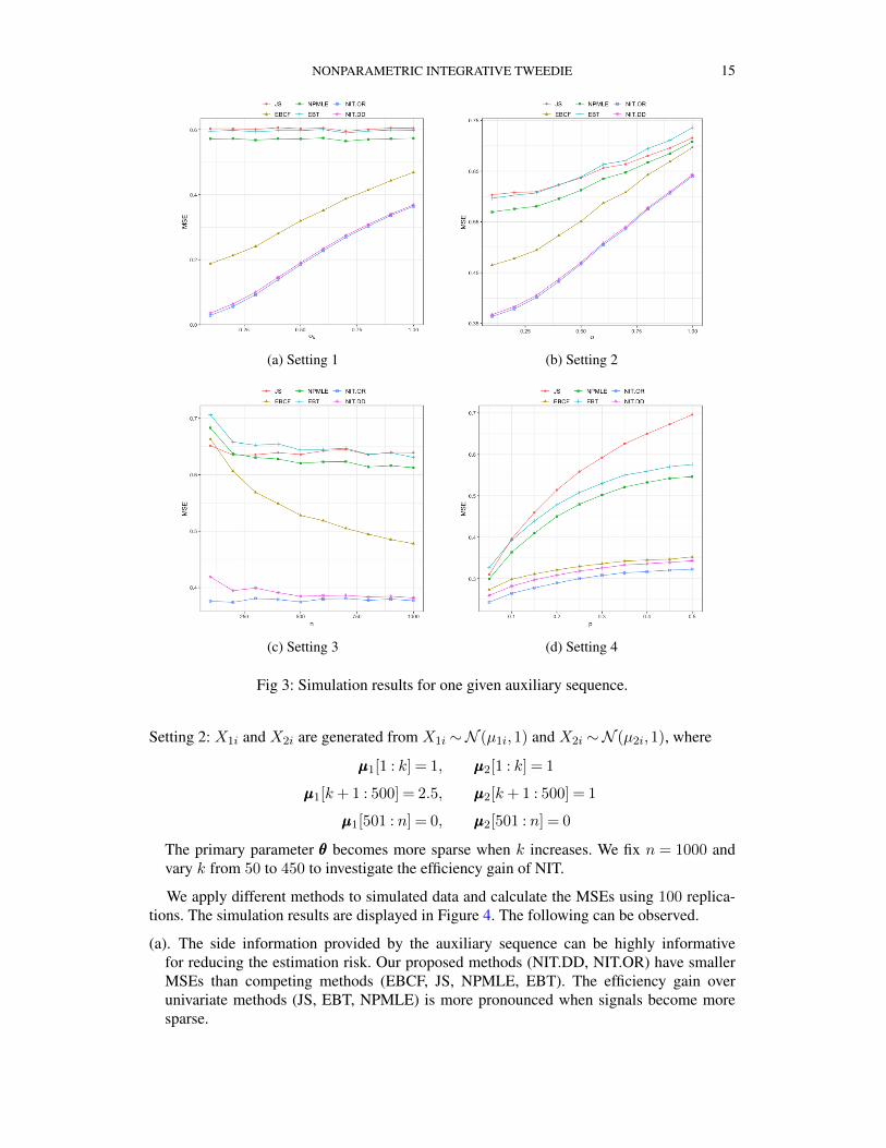
To illustrate the effectiveness of the integrative estimation strategy, we simulate dataaccording to the following two settings and obtain primary and auxiliary data as YYY ={X1i −X2i : 1≤ i≤ n and SSS = {X1i +X2i : 1≤ i≤ n}.Setting 1: X1i and X2i are generated from X1i ∼N (µ1i,1) and X2i ∼N (µ2i,1), where
µµµ1[1 : k] = 2.5, µµµ2[1 : k] = 1
µµµ1[k+ 1 : 2k] = 1, µµµ2[k+ 1 : 2k] = 1
µµµ1[2k+ 1 : n] = 0, µµµ2[2k+ 1 : n] = 0
The sparsity level of θθθ is controlled by k. We fix n= 1000 and vary k from 50 to 450 toinvestigate the impact of sparsity level on the efficiency of different methods.
3It can be shown that {(X1i−X2i,X1i+X2i) : 1≤ i≤ n} is minimal sufficient and retains all informationabout θθθ.
NONPARAMETRIC INTEGRATIVE TWEEDIE 15
(a) Setting 1 (b) Setting 2
(c) Setting 3 (d) Setting 4
Fig 3: Simulation results for one given auxiliary sequence.
Setting 2: X1i and X2i are generated from X1i ∼N (µ1i,1) and X2i ∼N (µ2i,1), where
µµµ1[1 : k] = 1, µµµ2[1 : k] = 1
µµµ1[k+ 1 : 500] = 2.5, µµµ2[k+ 1 : 500] = 1
µµµ1[501 : n] = 0, µµµ2[501 : n] = 0
The primary parameter θθθ becomes more sparse when k increases. We fix n = 1000 andvary k from 50 to 450 to investigate the efficiency gain of NIT.
We apply different methods to simulated data and calculate the MSEs using 100 replica-tions. The simulation results are displayed in Figure 4. The following can be observed.
(a). The side information provided by the auxiliary sequence can be highly informativefor reducing the estimation risk. Our proposed methods (NIT.DD, NIT.OR) have smallerMSEs than competing methods (EBCF, JS, NPMLE, EBT). The efficiency gain overunivariate methods (JS, EBT, NPMLE) is more pronounced when signals become moresparse.
16
(a) Setting 1 (b) Setting 2
Fig 4: Two-sample inference of sparse means.
(b). EBCF is dominated by NIT, and can be inferior to univariate shrinkage methods.(c). The class of linear estimators is inefficient under the sparse setting. For example, the
NPMLE method dominates the JS estimator, and the efficiency gain increases when thesignals become more sparse.
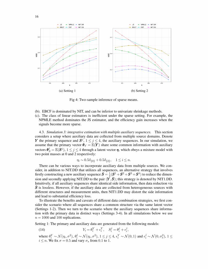
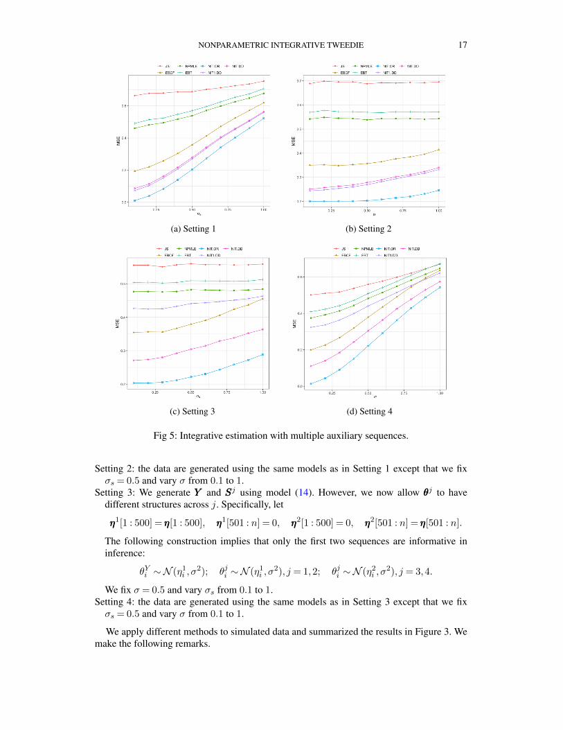
4.3. Simulation 3: integrative estimation with multiple auxiliary sequences. This sectionconsiders a setup where auxiliary data are collected from multiple source domains. DenoteYYY the primary sequence and SSSj , 1 ≤ j ≤ 4, the auxiliary sequences. In our simulation, weassume that the primary vector θθθY = E(YYY ) share some common information with auxiliaryvectors θθθjS = E(SSSj), 1≤ j ≤ 4 through a latent vector ηηη, which obeys a mixture model withtwo point masses at 0 and 2 respectively:
ηi ∼ 0.5δ{0} + 0.5δ{2}, 1≤ i≤ n.There can be various ways to incorporate auxiliary data from multiple sources. We con-
sider, in addition to NIT.DD that utilizes all sequences, an alternative strategy that involvesfirstly constructing a new auxiliary sequence SSS = 1
4(SSS1 +SSS2 +SSS3 +SSS4) to reduce the dimen-sion and secondly applying NIT.DD to the pair (YYY ,SSS); this strategy is denoted by NIT1.DD.Intuitively, if all auxiliary sequences share identical side information, then data reduction viaSSS is lossless. However, if the auxiliary data are collected from heterogeneous sources withdifferent structures and measurement units, then NIT1.DD may distort the side informationand lead to substantial efficiency loss.
To illustrate the benefits and caveats of different data combination strategies, we first con-sider the scenario where all sequences share a common structure via the same latent vector(Settings 1-2). Then we turn to the scenario where the auxiliary sequences share informa-tion with the primary data in distinct ways (Settings 3-4). In all simulations below we usen= 1000 and 100 replications.
Setting 1: The primary and auxiliary data are generated from the following models:
(14) Yi = θYi + εYi , Sji = θji + εji ,
where θYi ∼N (ηi, σ2), θji ∼N (ηi, σ
2), 1≤ j ≤ 4, εYi ∼N (0,1) and εji ∼N (0, σ2s), 1≤
i≤ n. We fix σ = 0.5 and vary σs from 0.1 to 1.
NONPARAMETRIC INTEGRATIVE TWEEDIE 17
(a) Setting 1 (b) Setting 2
(c) Setting 3 (d) Setting 4
Fig 5: Integrative estimation with multiple auxiliary sequences.
Setting 2: the data are generated using the same models as in Setting 1 except that we fixσs = 0.5 and vary σ from 0.1 to 1.
Setting 3: We generate YYY and SSSj using model (14). However, we now allow θθθj to havedifferent structures across j. Specifically, let
ηηη1[1 : 500] = ηηη[1 : 500], ηηη1[501 : n] = 0, ηηη2[1 : 500] = 0, ηηη2[501 : n] = ηηη[501 : n].
The following construction implies that only the first two sequences are informative ininference:
θYi ∼N (η1i , σ
2); θji ∼N (η1i , σ
2), j = 1,2; θji ∼N (η2i , σ
2), j = 3,4.
We fix σ = 0.5 and vary σs from 0.1 to 1.Setting 4: the data are generated using the same models as in Setting 3 except that we fixσs = 0.5 and vary σ from 0.1 to 1.
We apply different methods to simulated data and summarized the results in Figure 3. Wemake the following remarks.
18
(a). The univariate methods (JS, NPMLE, EBT) are dominated by the integrative methods(NIT.DD, NIT.OR, EBCF, NIT1.DD). The efficiency gain is more pronounced when σ andσs are small.
(b). EBCF is dominated by NIT.DD. Compared to the setting with one auxiliary sequence,the gap between the performances of NIT.OR and NIT.DD has widened because of theincreased complexity of the estimation problem in higher dimensions.
(c). In Settings 1-2, NIT1.DD is more efficient than NIT.DD as there is no loss in data re-duction and fewer sequences are utilized in estimation.
(d). In Settings 3-4, the average SSS does not provide an effective way to combine the infor-mation in auxiliary data. Since the last two sequences are not useful, such a data reductionstep leads to substantial information loss. NIT1.DD still outperforms univariate methodsbut is much worse than EBCF and NIT.DD.
The simulation results show that it is potentially beneficial to reduce the dimension ofauxiliary data. However, there can be significant information loss if the data reduction stepis carried out improperly. It would be of interest to develop principled methods for datareduction for extracting structural information from a large number of auxiliary sequences.
5. Applications. This section compares NIT and its competitors on gene expression dataand monthly sales data.
5.1. Integrative Non-parametric estimation of Gene Expressions. We consider the dataset in [36] that measures gene expression levels from cells that are without interferon alpha(INFA) protein and have been infected with varicella-zoster virus (VZV). VZV is known tocause chickenpox and shingles in humans [44]. INFA helps in host defense against VZVbut is often regulated in the presence of virus. Thus, it is important to estimate the geneexpressions in infected cells without INFA. Let θθθ be the true unknown vector of mean geneexpression values that need to be estimated. Further details about the dataset is provided inSection S.7.1 of the supplement.
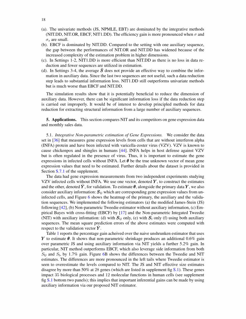
The data had gene expression measurements from two independent experiments studyingVZV infected cells without INFA. We use one vector, denoted YYY , to construct the estimatesand the other, denoted YYY , for validation. To estimate θθθ, alongside the primary data YYY , we alsoconsider auxiliary information:SSSU which are corresponding gene expression values from un-infected cells, and Figure 6 shows the heatmap of the primary, the auxiliary and the valida-tion sequences. We implemented the following estimators (a) the modified James-Stein (JS)following [42], (b) Non-parametric Tweedie estimator without auxiliary information, (c) Em-pirical Bayes with cross-fitting (EBCF) by [17] and the Non-parametric Integated Tweedie(NIT) with auxiliary infomation: (d) with SSSU only, (e) with SSSI only (f) using both auxiliarysequences. The mean square prediction errors of the above estimates were computed withrespect to the validation vector YYY .
Table 1 reports the percentage gain acheived over the naive unshrunken estimator that usesYYY to estimate θθθ. It shows that non-parametric shrinkage produces an additional 0.6% gainover parametric JS and using auxiliary information via NIT yields a further 5.2% gain. Inparticular, NIT method outperforms EBCF, which also leverage side information from bothSU and SI, by 1.7% gain. Figure 6B shows the differences between the Tweedie and NITestimates. The differences are more pronounced in the left tails where Tweedie estimator isseen to overestimate the levels compared to NIT. The JS and NIT effective size estimatesdisagree by more than 50% at 28 genes (which are listed in supplement fig S.1). These genesimpact 35 biological processes and 12 molecular functions in human cells (see supplementfig S.1 bottom two panels); this implies that important inferential gains can be made by usingauxiliary information via our proposed NIT estimator.
NONPARAMETRIC INTEGRATIVE TWEEDIE 19
Fig 6: Panel A: Heatmaps of the gene expression datasets showing the four expression vectorscorresponding to the observed, validation and auxiliary sequences. Panel B: scatterplot of theeffect size estimates of gene expressions based on Tweedie and NIT (using both SU and SI).Magnitude of the auxiliary variables used in the NIT estimate is reflected by different colors.
TABLE 1% gain in prediction errors by different estimators over the naive unshrunken estimator of gene expressions of
INFA regulated infected cells.
Methods James-Stein Tweedie EBCF using SSSU & SSSI NIT using SSSU NIT using SSSI NIT using SSSU & SSSI
% Gain 3.5 4.1 7.6 6.9 7.5 9.3
MSE 2.014 2.001 1.927 1.930 1.951 1.895
5.2. Leveraging auxiliary information in predicting monthly sales. We consider the totalmonthly sales of beers across n= 866 stores of a retail grocery chain. These stores are spreadacross different states in the USA (see Figure S.2 in the Supplement). The data is extractedfrom [5], which has been widely studied for inventory management and consumer preferenceanalyses; see also [4] and the references therein.
Let YYY t be the n dimensional vector denoting the monthly sales of beer across the n storesin month t ∈ {1, . . . ,12}. For inventory planning, it is economically important to estimatefuture demand. In this context, we consider estimating the monthly demand vector (acrossstores) for month t using the previous month’s sales YYY t−1. We use the first six months t =1, . . . ,6 for estimating store demand variabilities σ2
i , i = 1, . . . , n. For t = 7, . . . ,12, usingestimators based on month t’s sales, we calculate their demand prediction error for montht+ 1 by using its monthly sale data for validation. Among the estimators, we introspect themodified James-Stein (JS) estimator of Xie, Kou and Brown [42]:
θθθt+1
i [JS] = JSt
i +
[1− n− 3∑
i σ−2i (Y t
i − JSt
i)2
]+
(Y ti − JS
t
i) where JSt
i =
∑ni=1 σ
−2i Y t
i∑ni=1 σ
−2i
,
as well as the Tweedie (T) estimator θθθt+1
i [T] = Y ti + σihi where hi are estimates of
∇1 log f(σ−1i Y t
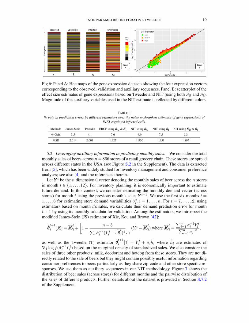
i ) based on the marginal density of standardized sales. We also consider thesales of three other products: milk, deodorant and hotdog from these stores. They are not di-rectly related to the sale of beers but they might contain possibly useful information regardingconsumer preferences to beers particularly as they share zip-code and other store specific re-sponses. We use them as auxiliary sequences in our NIT methodology. Figure 7 shows thedistribution of beer sales (across stores) for different months and the pairwise distribution ofthe sales of different products. Further details about the dataset is provided in Section S.7.2of the Supplement.
20
Fig 7: Distribution of monthly sales of beer across stores (on left) and the pairwise distribu-tion of joint sales of different products in the month of July (in right).
In Table 2, we report the average % gain in predictive error by the James-Stein (JS),Tweedie (T) and integrative Tweedie (IT) estimators (using different combinations of aux-iliary sequences) over the naive estimator δt+1,naive =YYY t for the demand prediction problemat t = 7, . . . ,12. The detailed month-wise gains and the loss function are provided in thesupplement. Using auxiliary variables via our proposed NIT framework yields significantadditional gains over non-integrative methods. However, the improvement slackens as an in-creasing number of auxiliary sequences are incorporated. It is to be noted that the demanddata set is highly complex and heterogeneous and n = 866 may not be adequately largefor conducting successful non-parametric estimation. Hence suitably anchored parametric JSestimator produces better prediction than non-parmatric Tweedie. Also, as demonstrated inTable S.2 of the Supplement, there are months where shrinkage estimation methods do notyield positive gains. Nonetheless, the NIT estimator produces significant advantages overcompeting methods. It produces on average 7.7% gain over unshrunken methods and attainsan additional 3.7% gain over non-parametric shrinkage methods.
TABLE 2Average % gains over the naive unshrunken estimator for monthly beer sales prediction
JS Tweedie IT-Milk IT-Deodorant IT-Hotdog IT-M&D IT-M&H IT-D&H IT-M&D&H
5.7 4.0 6.0 7.1 6.8 6.1 6.6 7.5 7.7
6. Discussion. NIT, inspired by classical empirical Bayes ideas, provides a new frame-work for transferring useful structural knowledge from related sources domains to assist theestimation of a high-dimensional parameter in the target domain. The framework avoids neg-ative learning because no distributional assumptions are imposed on auxiliary data SSS, whichare allowed to be categorical, numerical or of mixed type. The auxiliary data are only used toprovide structural knowledge of the high-dimensional parameter in the target domain.
Our theory tabulates the reductions in estimation errors and deteriorations in the learn-ing rates as the dimension of SSS increases. This indicates that if we have a large number ofvariables as potential choices for auxiliary data, it would be beneficial to first conduct datareduction before applying the NIT estimator. The loss of information resulted from the datareduction process can possibly be compensated by the increased precision in the optimiza-tion process. However, our simulation results in Section 4.3 show that there can be significant

NONPARAMETRIC INTEGRATIVE TWEEDIE 21
information loss if the data reduction step is carried out improperly. Our findings suggest twodirections for future research: (a) the investigation of the tradeoff, as K increases, betweenthe achievable error limit of the oracle rule and the decreased convergence rate of the data-driven rule, and (b) the development of principled structure-preserving dimension reductionmethods under the transfer learning framework for extracting useful structural informationfrom a large number of auxiliary sequences.
REFERENCES
[1] BANERJEE, T., MUKHERJEE, G. and SUN, W. (2020). Adaptive sparse estimation with side information.Journal of the American Statistical Association 115 2053-2067.
[2] BANERJEE, T., LIU, Q., MUKHERJEE, G. and SUN, W. (2021). A General Framework for Empirical BayesEstimation in Discrete Linear Exponential Family. Journal of Machine Learning Research 22 1-46.
[3] BENJAMINI, Y. and HOCHBERG, Y. (1995). Controlling the false discovery rate: a practical and powerfulapproach to multiple testing. J. Roy. Statist. Soc. B 57 289–300. MR1325392 (96d:62143)
[4] BRONNENBERG, B. J., DUBÉ, J.-P. H. and GENTZKOW, M. (2012). The evolution of brand preferences:Evidence from consumer migration. American Economic Review 102 2472–2508.
[5] BRONNENBERG, B. J., KRUGER, M. W. and MELA, C. F. (2008). Database paper—The IRI marketingdata set. Marketing science 27 745–748.
[6] BROWN, L. D. (1971). Admissible estimators, recurrent diffusions, and insoluble boundary value problems.The Annals of Mathematical Statistics 42 855–903.
[7] BROWN, L. D. and GREENSHTEIN, E. (2009). Nonparametric empirical Bayes and compound decisionapproaches to estimation of a high-dimensional vector of normal means. The Annals of Statistics 371685–1704.
[8] BROWN, L. D., GREENSHTEIN, E. and RITOV, Y. (2013). The Poisson compound decision problem revis-ited. Journal of the American Statistical Association 108 741–749.
[9] CAI, T. T., SUN, W. and WANG, W. (2019). CARS: Covariate assisted ranking and screening for large-scaletwo-sample inference (with discussion). J. Roy. Statist. Soc. B 81 187–234.
[10] CHWIALKOWSKI, K., STRATHMANN, H. and GRETTON, A. (2016). A kernel test of goodness of fit. JMLR:Workshop and Conference Proceedings.
[11] COHEN, N., GREENSHTEIN, E. and RITOV, Y. (2013). Empirical Bayes in the presence of explanatoryvariables. Statistica Sinica 333–357.
[12] EFRON, B. (2011). Tweedie’s Formula and Selection Bias. Journal of the American Statistical Association106 1602–1614.
[13] EFRON, B., TIBSHIRANI, R., STOREY, J. D. and TUSHER, V. (2001). Empirical Bayes analysis of a mi-croarray experiment. J. Amer. Statist. Assoc. 96 1151–1160. MR1946571
[14] GRETTON, A., BORGWARDT, K. M., RASCH, M. J., SCHÖLKOPF, B. and SMOLA, A. (2012). A kerneltwo-sample test. The Journal of Machine Learning Research 13 723–773.
[15] GU, J. and KOENKER, R. (2017). Unobserved heterogeneity in income dynamics: An empirical Bayesperspective. Journal of Business & Economic Statistics 35 1–16.
[16] IGNATIADIS, N. and HUBER, W. (2020). Covariate powered cross-weighted multiple testing. arXiv preprintarXiv:1701.05179.
[17] IGNATIADIS, N. and WAGER, S. (2019). Covariate-Powered Empirical Bayes Estimation. In Advances inNeural Information Processing Systems 9617–9629.
[18] IGNATIADIS, N., SAHA, S., SUN, D. L. and MURALIDHARAN, O. (2019). Empirical Bayes mean estima-tion with nonparametric errors via order statistic regression. arXiv preprint arXiv:1911.05970.
[19] JIANG, W. and ZHANG, C.-H. (2009). General maximum likelihood empirical Bayes estimation of normalmeans. The Annals of Statistics 37 1647–1684.
[20] JING, B.-Y., LI, Z., PAN, G. and ZHOU, W. (2016). On sure-type double shrinkage estimation. Journal ofthe American Statistical Association 111 1696–1704.
[21] KE, T., JIN, J. and FAN, J. (2014). Covariance assisted screening and estimation. Annals of statistics 422202-2242.
[22] KOENKER, R. and GU, J. (2017). REBayes: An R Package for Empirical Bayes Mixture Methods. Journalof Statistical Software 82 1–26.
[23] KOENKER, R. and MIZERA, I. (2014). Convex optimization, shape constraints, compound decisions, andempirical Bayes rules. Journal of the American Statistical Association 109 674–685.
[24] KOU, S. and YANG, J. J. (2017). Optimal shrinkage estimation in heteroscedastic hierarchical linear mod-els. In Big and Complex Data Analysis 249–284. Springer.

22
[25] KRUSINSKA, E. (1987). A valuation of state of object based on weighted Mahalanobis distance. PatternRecognition 20 413–418.
[26] LEI, L. and FITHIAN, W. (2018). AdaPT: an interactive procedure for multiple testing with side information.Journal of the Royal Statistical Society: Series B (Statistical Methodology) 80 649–679.
[27] LI, A. and BARBER, R. F. (2019). Multiple testing with the structure-adaptive Benjamini–Hochberg algo-rithm. Journal of the Royal Statistical Society: Series B (Statistical Methodology) 81 45–74.
[28] LIU, Q., LEE, J. and JORDAN, M. (2016). A kernelized Stein discrepancy for goodness-of-fit tests. Inter-national conference on machine learning 276–284.
[29] LIU, Q. and WANG, D. (2016). Stein variational gradient descent: A general purpose bayesian inferencealgorithm. In Advances in neural information processing systems 2378–2386.
[30] OATES, C. J., GIROLAMI, M. and CHOPIN, N. (2017). Control functionals for Monte Carlo integration.Journal of the Royal Statistical Society: Series B (Statistical Methodology) 79 695–718.
[31] REN, Z. and CANDÈS, E. (2020). Knockoffs with side information. arXiv preprint arXiv:2001.07835.[32] ROBBINS, H. (1951). Asymptotically subminimax solutions of compound statistical decision problems.
In Proceedings of the Second Berkeley Symposium on Mathematical Statistics and Probability, 1950131–148. University of California Press, Berkeley and Los Angeles. MR0044803 (13,480d)
[33] ROBBINS, H. (1964). The empirical Bayes approach to statistical decision problems. The Annals of Mathe-matical Statistics 35 1–20.
[34] ROEDER, K. and WASSERMAN, L. (2009). Genome-wide significance levels and weighted hypothesis test-ing. Statistical science: a review journal of the Institute of Mathematical Statistics 24 398.
[35] SAHA, S. and GUNTUBOYINA, A. (2020). On the nonparametric maximum likelihood estimator for Gaus-sian location mixture densities with application to Gaussian denoising. Annals of Statistics 48 738–762.
[36] SEN, N., SUNG, P., PANDA, A. and ARVIN, A. M. (2018). Distinctive roles for type I and type II interfer-ons and interferon regulatory factors in the host cell defense against varicella-zoster virus. Journal ofvirology 92 e01151–18.
[37] SERFLING, R. J. (2009). Approximation Theorems of Mathematical Statistics. Wiley Series in Probabilityand Statistics. Wiley.
[38] STEIN, C. (1956). Inadmissibility of the usual estimator for the mean of a multivariate normal distributionTechnical Report, STANFORD UNIVERSITY STANFORD United States.
[39] SUN, W. and CAI, T. T. (2007). Oracle and adaptive compound decision rules for false discovery ratecontrol. J. Amer. Statist. Assoc. 102 901–912. MR2411657
[40] TAN, Z. (2015). Improved minimax estimation of a multivariate normal mean under heteroscedasticity.Bernoulli 21 574–603.
[41] WEINSTEIN, A., MA, Z., BROWN, L. D. and ZHANG, C.-H. (2018). Group-linear empirical Bayes esti-mates for a heteroscedastic normal mean. Journal of the American Statistical Association 113 698–710.
[42] XIE, X., KOU, S. and BROWN, L. D. (2012). SURE estimates for a heteroscedastic hierarchical model.Journal of the American Statistical Association 107 1465–1479.
[43] YANG, J., LIU, Q., RAO, V. and NEVILLE, J. (2018). Goodness-of-fit testing for discrete distributions viaStein discrepancy. In International Conference on Machine Learning 5557–5566.
[44] ZERBONI, L., SEN, N., OLIVER, S. L. and ARVIN, A. M. (2014). Molecular mechanisms of varicellazoster virus pathogenesis. Nature reviews microbiology 12 197–210.
[45] ZHANG, C.-H. (1997). Empirical Bayes and compound estimation of normal means. Statistica Sinica 7181–193.
[46] ZHANG, X. and BHATTACHARYA, A. (2017). Empirical bayes, sure and sparse normal mean models. arXivpreprint arXiv:1702.05195.

Supplementary Material for “Transfer Learning for Empirical
Bayes Estimation: a Nonparametric Integrative Tweedie
Approach”
Jiajun Luo, Gourab Mukherjee and Wenguang Sun
University of Southern California
In Sections S.1-S.6 of this supplement we present the proofs of all results stated in the main paper.
The proofs are presented in the order the results appear in the main paper. The equations and results
that only appear in the supplement but not in the main paper are prefixed by S. We also provide further
details regarding the real data examples Section S.7.
S.1 Proof of Proposition 1
The idea of the proof follows from Brown [1971]; we provide it here for compeleteness.
Noting that f(y,sss) =∫f(y,sss|θ)dhθ(θ) and f(y,sss|θ) = f(y|sss, θ)f(sss|θ), expand the partial
derivative of f(y,sss):
∇yf(y,sss) = σ−2(∫
θf(y|sss, θ)f(sss|θ)dhθ(θ)− y∫f(y|sss, θ)f(sss|θ)dhθ(θ)
)= σ−2
(∫θf(y,sss|θ)dhθ(θ)− yf(y,sss)
)Then, left-multiplying by σ2 and dividing by f(y,sss) on both sides, it follows that
σ2∇yf(y,sss)
f(y,sss)=
∫θf(y,sss|θ)dhθ(θ)f(y,sss|θ)
− y
Under square error loss, the posterior mean minimizes the Bayes risk. And so, the Bayes estimator is
given by
E(θ|y,sss) =
∫θf(y,sss|θ)dhθ(θ)
f(y,sss)= y + σ2
∇yf(y,sss)
f(y,sss),
where, the second equality follows from the above two displays.
1

S.2 Proof of Theorem 1
First note that the expected value of the concerned `p distance
`p(hhhλ,n, hf ) = n−1n∑i=1
|hhhλ,n(i)− hf (xxxi)|p
is given by ∆(p)λ,n(f) = EXXX{`p(hhhλ,n, hf )} where, the expected value is over XXXn = (xxx1;xxx2; . . . ;xxxn)
where xxxis are i.i.d. from f . Thus,
∆(p)λ,n(f) = E |hhhλ,n(1)− hf (xxx1)|p = E|hhhλ[XXXn](xxx1)− hf (xxx1)|p .
For notational ease, we would often keep the dependence on f in ∆(p)λ,n(f) implicit. The proof involves
upper and lower bounding ∆(2)λ,n by the functionals involving ∆
(1)λ,n. The upper bound is provided
below in (S.3). The lower bound follows from (S.5), whose proof is quite convoluted and is presented
separately in Lemma S.2.1.
As the marginal density of the θθθ is the convolution with a Gaussian distribution, it follows that
there exists some constant C ≥ 0 such that
|hf (xxx1)|/‖xxx1‖2 ≤ C for all large ||xxx1||2.
and |hhhλ[XXXn](xxx1)| = O(‖xxx1‖2). With out loss of generality we include such constraints on hhh in the
convex program to solve (5) and so, |hhhλ[XXXn](xxx1)− hf (xxx1)| is also bounded by O(‖xxx1‖2).
Using this property of the score estimates, we have the following bound for all xxx1 satisfying
{xxx1 : ‖xxx1‖2 ≤ 2γ log n}:
E[(hhhλ[XXXn](xxx1)− hf (xxx1)
)2I {‖xxx1‖2 ≤ 2γ log n}
]≤ 2γ log(n) ∆
(1)λ,n. (S.1)
On the set {‖xxx1‖2 > 2γ log n}, again using the aforementioned property of score estimates from (5)
we note that
E[(hhhλ[XXXn](xxx1)− hf (xxx1)
)2I {‖xxx1‖2 > 2γ log n}
]. E
[‖xxx1‖22I{‖xxx1‖2 > 2γ log n}
], (S.2)
where, for any two sequences an, bn, we use the notation an . bn to denote an/bn = O(1) as n→∞.
Now, as xxx1 satisfies assumption 1, the right hand side (S.2) is bounded by O(n−1). Combining
(S.1) and (S.2) we have the following upper bound on ∆(2)λ,n:
∆(2)λ,n . log(n) ∆
(1)λ,n + n−1 . (S.3)
2

For the lower bound on ∆(2)λ,n consider the following intermediate quantity which is related to the
KSD norm dλ on the score functions:
∆λ,n(f) = E{(hhhλ[XXXn](xxx1)− hf (xxx1)
)2f(xxx1)
}.
It can be shown that
∆(1)λ,n .
√{log(n)}K+1 ∆λ,n + n−1 as n→∞. (S.4)
Proof of (S.4). Restrictingxxx1 on set {xxx1 : ‖xxx1‖2 ≤ 2γ log n} and using Cauchy-Schwarz inequal-
ity, we get
E[(hhhλ[XXXn](xxx1)− hf (xxx1)
)2I {‖xxx1‖2 ≤ 2γ log n}
]≤[CK,γ {log(n)}K+1∆λ,n(f)
] 12 .
On the tail {xxx1 : ‖xxx1‖2 > 2γ log n} using the same argument as (S.2), we have
E[∣∣∣hhhλ[XXXn](xxx1)− hf (xxx1)
∣∣∣ I {‖xxx1‖2 > 2γ log n}]
= O(n−1).
(S.4) follows by combining the above two displays.
The following result lower bounds ∆(2)λ,n using ∆λ,n.
Lemma S.2.1. For any λ > 0, we have
∆λ,n . λ−(K+1)Sλ[hhhλ,n+1] + λ2 log n+ λ(log n)K+3∆(2)λ,n . (S.5)
The proof of the above lemma is intricate and is presented at the end of this section.
Now, for the proof of theorem 1, we combine (S.3), (S.4) and (S.5). Then, using λ � n−1
K+2 and
the fact that ∆(1)λ,n is bounded, we arrive at
∆(1)λ,n .
√{log(n)}K+1
{nK+1K+2Sλ[hhhλ,n+1] + n−
2K+2 log(n) + n−
1K+2 (log n)K+4 ∆
(1)λ,n
}. (S.6)
Proportion S.2.2, which is stated and proved at the end of this proof, provides the following upper
bound on Sλ[hhhλ,n+1]:
Sλ[hhhλ,n+1] ≤E {hf (xxx1)}2 − E
{hhhλ[XXXn+1](xxx1)
}2
n(S.7)
3

Using the similar argument as (S.3), the numerator in above can be further upper bounded by 2γ∆(1)λ,n+1+
O(n−1). Substituting this in (S.6), we arrive at an inequality only involving quantities ∆(1)λ,n and
∆(1)λ,n+1. Now, noting that λ � n−
1K+2 and ∆
(1)λ,n is bounded, it easily follows that ∆
(1)λ,n → 0 as
n→∞.
Establishing the rate of convergence of ∆(1)λ,n needs further calculations. For that purpose consider
An = max{
∆(1)λ,n, 2n−
1K+2 (log n)2K+5
}. For all large n, the following inequality can be derived
from (S.6) and (S.7):
An ≤ C (log n)K+1n−1
2K+4
√An+1, (S.8)
where C is a constant independent of n.
Applying (S.8) recursively m times we have:
An ≤(C(log n)K+1n−
12K+4
)1+···+ 12m
A1
2m+1
n+m+1.
Note that An < 1 for all large n. This implies that for any m > 0,
An ≤(C(log n)K+1n−
12K+4
)1+···+ 12m
.
Finally, let m→∞, we proved that An ≤ C(log n)2K+2n−1
K+2 , which implies
∆(1)λ,n . (log n)2K+2n−
1K+2 .
This completes the proof of Theorem 1.
S.2.1 Proofs of results used in the proof of Theorem 1
Proposition S.2.2. Let Kλ(·, ·) be RBF kernel with bandwidth parameter λ ∈ Λ and Λ is a compact
set of R+ bounded from zero. Then we have
Sλ[hhhλ,n] ≤E {hf (xxx1)}2 − E
{hhhλ[XXXn](xxx1)
}2
n− 1.
Proof of Proposition S.2.2. By the construction of the hhhλ,n, we have
Sλ[hhhλ,n] ≤ Sλ[hhhf ]. (S.9)
4

Taking the expectation on the both sides of equation (S.9), we get
n2 − nn2
Sλ[hhhλ,n] +n
n2
(E{hhhλ[XXXn](xxx1)
}2+
1
λ
)≤ n2 − n
n2Sλ[hf ] +
n
n2
(E {hf (xxx1)}2 +
1
λ
).
Notice that Sλ[hf ] = 0 and then the above inequality implies
Sλ[hhhλ,n] ≤E {hf (xxx1)}2 − E
{hhhλ[XXXn](xxx1)
}2
n− 1,
which completes the proof.
Proof of Lemma S.2.1.
First we assume there are n + 1 i.i.d. samples, XXXn+1 = (xxx1;xxx2; . . . ;xxxn+1) where xxxis are i.i.d. from
f . Note that the definition of Sλ[hhhλ,n+1] is equivalent to the following definition:
Sλ[hhhλ,n+1] = E [Dλ(xxx1,xxxn+1)] ,
where the KSD is given by
Dλ(xxx1,xxxn+1) = Kλ(xxx1,xxxn+1)(hhhλ[XXXn+1](xxx1)− hf (xxx1)
)(hhhλ[XXXn+1](xxxn+1)− hf (xxxn+1)
).
We consider the situation when xxxn+1 is in the ε-neighboor of xxx1. For a fixed ε > 0, denote
I(1)ε;λ := E
[Dλ(xxx1,xxxn+1)I{‖xxxn+1 − xxx1‖ < ε}
].
When ε = λ log n, we have
I(1)ε;λ ≤ Sλ[hhhλ,n+1] +O
(n−0.5 logn
). (S.10)
The proof of (S.10) is non-trivial. To avoid disrupting the flow of arguments here, its proof is not
presented immediately but is provided at the end of this subsection.
Denote the following intermediate quantity I(2)ε;λ which is close to ∆λ,n(f) as
I(2)ε;λ := E
[Kλ(xxx1,xxxn+1)
(hhhλ[XXXn+1](xxx1)− hf (xxx1)
)2I{‖xxxn+1 − xxx1‖ < ε}
].
We use Cauchy Schwarz inequality and lipschitz continuity of score function to show I(2)ε;λ is bounded
5

by a function of I(1)ε;λ as
I(2)ε;λ ≤ I
(1)ε;λ +O(εK+3). (S.11)
The proof of (S.11) is quite involved and is presented afterwards. Finally, we establish the following
bound which along with (S.10) and (S.11) complete the proof of the lemma:
∆λ,n . λ−K−1I(2)ε;λ + λ2(log n)K+3 + λ∆
(2)λ,n log n. (S.12)
Proof of (S.10). Note that the difference between Sλ[hhhλ,n+1] and I(1)ε;λ is
E[Dλ(xxx1,xxxn+1)I{‖xxxn+1 − xxx1‖ ≥ ε}
].
If we use the Gaussian kernal Kλ(xxx1,xxxn+1) = e−1
2λ2‖xxx1−xxxn+1‖2 and set ε = λ log n, we have
Kλ(xxx1,xxxn+1)I{‖xxxn+1 − xxx1‖ ≥ ε} is always bounded by n−0.5 logn, which implies the above dif-
ference is bounded by ∆(2)λ,n+1n
−0.5 logn. Note that ∆(2)λ,n+1 is bounded, (S.10) follows.
Proof of (S.11). Note that the score function hf is Lf -Lipschitz continuous. If we assume for
small ε, when ‖xxxn+1 − xxx1‖ < ε, we have hhhλ[XXXn+1](xxxn+1) is Ln,ε-Lipschitz continuous as∣∣∣hhhλ[XXXn+1](xxxn+1)− hhhλ[XXXn+1](xxx1)∣∣∣ ≤ Ln,ε ε. (S.13)
where Ln,ε satisfies that EL2n,ε is bounded. Then the difference between I(2)ε;λ and I(1)ε;λ is bounded by
E[ε (Lf + Ln,ε)Kλ(xxx1,xxxn+1)
∣∣∣hhhλ[XXXn+1](xxx1)− hf (xxx1)∣∣∣ I{‖xxxn − xxx1‖ < ε}
]Apply the Cauchy-Schwarz inequality and the square of above difference can be further bounded by
εE[(Lf + Ln,ε)
2I{‖xxxn − xxx1‖ < ε}]E[K2λ(xxx1,xxxn+1)
∣∣∣hhhλ[XXXn+1](xxx1)− hf (xxx1)∣∣∣2 I{‖xxxn − xxx1‖ < ε}
]Note that E
[(Lf + Ln,ε)
2I{‖xxxn − xxx1‖ < ε}]
is bounded by
Cfπ(K+1)/2
Γ(K+12 + 1)
εK+1E(Lf + Ln,ε)2,
where Γ(x) is the gamma function. Notice that K2λ(xxx1,xxxn+1) ≤ Kλ(xxx1,xxxn+1) and then we have
I(2)ε;λ . I
(1)ε;λ + ε
√εK+1∆2
ε;λ.
6

This completes the proof of (S.11).
Proof of (S.12). We introduce an intermediate quantity:
I(3)ε;λ = E
[Kλ(xxx1,xxxn+1)
(hhhλ[XXXn](xxx1)− hf (xxx1)
)2I{‖xxxn+1 − xxx1‖ < ε}
].
Assume that when n is large and ‖xxxn+1 − xxx1‖ < ε, we have hhhλ[XXXn+1](xxxn+1) is Ln,ε-Lipschitz
continuous as: ∣∣∣hhhλ[XXXn+1](xxxn+1)− hhhλ[XXXn](xxx1)∣∣∣ ≤ Ln,ε ε
Combined with (S.13), we get the difference between I(3)ε;λ and I(2)ε;λ is bounded by
4ε2 E[L2n,εKλ(xxx1,xxxn+1)I{‖xxxn+1 − xxx1‖ < ε}
],
which implies that
I(3)ε;λ . I
(2)ε;λ + εK+3. (S.14)
Next we introduce another intermediate quantity
I(4)ε;λ = E
∫f(xxx1)Kλ(xxx1,xxxn+1)
(hhhλ[XXXn](xxx1)− hf (xxx1)
)2I{‖xxxn+1 − xxx1‖ < ε} dxxxn+1,
which is close to I(3)ε;λ . When ε = λ log n, we have the following term∫Kλ(xxx1,xxxn+1)I{‖xxxn+1 − xxx1‖ < ε} dxxxn+1
is lower bounded by
λK+1
∫e−
12‖xxxn+1‖2I{‖xxxn+1‖ < log n} dxxxn+1,
which can be further lower bounded by c λK+1 for some constant c when n is large. This implies
λK+1 ∆λ,n(f) . I(4)ε;λ . (S.15)
Now it is enough to show I(4)ε;λ . I
(3)ε;λ + λK+2∆
(2)λ,n log n.
Assume that f is Lf -Lipschitz continuous. The difference between I(4)ε;λ and I(3)ε;λ is bounded by
Lf ε∆(2)λ,n
∫[Kλ(xxx1,xxxn+1)I{‖xxxn+1 − xxx1‖ < ε}] dxxxn+1.
7

Notice that∫
[Kλ(xxx1,xxxn+1)I{‖xxxn+1 − xxx1‖ < ε}] dxxxn+1 is bounded by C λK+1 for some constant
C. This implies that
I(4)ε;λ . ∆3
ε;λ + λK+2I(3)λ,n log n.
Combined with (S.14) and (S.15), the result (S.12) follows.
S.3 Proof of Lemma 2
We follow the notions in Section S.2. The convergence rate of ∆(2)λ,n is achieved by extending the
results of ∆(1)λ,n in Section S.2. Recall that (S.3) shows
∆(2)λ,n . log(n) ∆
(1)λ,n + n−1 ,
and we have proved ∆(1)λ,n . (log n)2K+2n−
1K+2 in Section S.2. Combining these two, we obtain the
result stated in this lemma.
S.4 Proof of Proposition 2
Proposition 4.5 in Johnstone [2011] shows that Bn(δδδπ(yyy)) = σ2 − σ4IY . Following the same argu-
ments, we have Bn(δδδπ(yyy,SSS)) = σ2 − σ4I(py|sss). Then it follows
Bn(δδδπ(yyy))−Bn(δδδπ(yyy,SSS)) = σ4(IY |SSS − IY )
Next, we prove that IY |SSS − IY is non-negative. By the definition of IY |SSS , we have the following
decomposition:
IY |SSS =
∫∫ (f(y)∇yf(sss|y) + f(sss|y)∇yf(y)
f(y,sss)
)2f(y,sss) dy dsss.
Then we break the square and it follows
IY |SSS =
∫∫ (∇yf(sss|y)
f(sss|y)
)2f(y,sss) dy dsss+
∫∫ (∇yf(y)
f(y)
)2f(y) dy + 2
∫∫∇yf(sss|y)∇yf(y) dy dsss.
Note that the second term of right hand side is always non-negative. Then we consider the last term
and exchange the integration and partial derivative, we get∫∫∇yf(sss|y)∇yf(y) dy dsss =
∫∇yf(y)∇y
(∫f(sss|y)dsss
)dy = 0
It follows that IY ≥ IY |SSS .
8

S.5 Proof of Theorem 3
The proof of this theorem follows along the similar lines of the proof for Theorem 1. Denote α =
1/(3(K + 1)(K + 2)). In this case we entertain the possiblity that the joint density f can be a heavier
tailed density. We concentrate on set {‖xxx1‖2 ≤ nα} instead of the set {‖xxx1‖2 . log n} analyzed in
the proof of Theorem 1.
Noting that hhhλ[XXXn](xxx1) and hf (xxx1) are bothO (1) it follows that |hhhλ[XXXn](xxx1)−hf (xxx1)| = O (1).
Then applying the Cauchy-Schwarz inequality, we get
E[(hhhλ[XXXn](xxx1)− hf (xxx1)
)2I {‖xxx1‖2 ≤ n
α}].{n(K+1)α ∆λ,n
}1/2. (S.16)
Next, we consider the situation when ||xxxi||2 is large. Using |hhhλ[XXXn](xxx1) − hf (xxx1)| = O (1) and
Assumption 2, it follows
E[(hhhλ[XXXn](xxx1)− hf (xxx1)
)2I {‖xxx1‖2 > nα}
]. n−α(K+1) . (S.17)
Combining (S.16) and (S.17) gives the bound on ∆(2)λ,n as
∆(2)λ,n .
{n(K+1)α ∆λ,n
}1/2+ n−α(K+1) . (S.18)
Now, recall (S.5) in Lemma S.2.1 upper bounds ∆λ,n by a function of ∆(2)λ,n. Using (S.5) and (S.18),
we get
∆(2)λ,n . n(K+1)α/2
{λ−(K+1)Sλ[hhhλ,n+1] + λ2 log n+ λ(log n)K+3∆
(2)λ,n
}1/2+ n−α(K+1) .
(S.19)
Note that, ∆(2)λ,n is bounded and so, Proposition S.2.2 implies Sλ[hhhλ,n+1] is bounded by O(n−1).
Finally, let λ � Θ(n−1
K+2 ) and substitute α = 13(K+1)(K+2) in (S.19) to obtain
∆(2)λ,n . n
− 13(K+2) ,
which completes the proof of Theorem 3.
9

S.6 Proof of Proposition 3
First note that
Kλ ((ui, si); (uj , sj)) /Kλ ((xi, si); (xj , sj)) = exp
{− 1
2λ(ui − uj)2 +
1
2λ(xi − xj)2
}= exp
{− 1
2λ
[α2(ηi − ηj)2 − 2α(ηi − ηj)(xi − xj)
]}:= I1.
For any fixed n, we have xmax − xmin ≤ C1 and ηmax − ηmin ≤ C2 for some quantities C1 and C2.
Then the above is bounded by
I2 := exp{−2−1λ−1α(C2
2α− 2C1C2)}.
The above ratio for∇Kλ equals I1(ui − uj)/(xi − xj), which is bounded in magnitude by I2 (C3 + C2)/C3
where C3 = mini 6=j |xi − xj | and C3 > 0 as the distribution of Y in (1) is continuous.
Now consider the estimators
δITλ,i(U, S) = ui + σ2(1 + α2)gi = yi + αηi + σ2(1 + α2)gi, and,
δITλ,i(Y, S) = yi + σ2(1 + α2)hi ,
where, for an arbitrary fixed value of λ, gi and hi are solutions from (5) using (u, s) and (y, s) respec-
tively. Note that,
Ln(λ, α) =1
n
∑i
(δITλ,i(U, S)− vi
)2− σ2(1 + α−2).
Taking expectation and using the fact that V is conditionally independent of (U, S), we get,
E{Ln(λ, α)} = E
[1
n
∑i
(δITλ,i(U, S)− θi
)2].
For any fixed n,
Di := δITλ,i(U, S)− δIT
λ,i(U, S) = αηi + σ2[(1 + α2)gi − hi
].
Now, if the optimization in (5) is strictly convex, then for any small α, there exists εα such that
maxi |gi − hi| < εα and εα ↓ 0 as α ↓ 0 and the result stated in this proposition follows.
10
S.7 Further details on the Real Data Illustrations
S.7.1 Gene Expressions Estimation example
The data considered in this analysis was collected in Sen et al. [2018] via RNA sequencing. The set
of genes in the sequencing kit was same across all the experiments. The standard deviations of the
expressions values corresponding to the different genes were estimated from related gene expression
samples which contain replications under different experimental conditions. Pooling data across these
experiments, unexpressed and lowly expressed genes were filtered out. The resultant data consist of
around 30% of the genes. We consider the estimation of the mean expression levels of n = 3000
genes. The primary parameter θθθ is estimated based on primary vector YYY and two auxiliary sequences
SSSU and SSSI.
In Figure S.1 (top panel), we list the 28 genes for which the Tweedie and integrative Tweedie esti-
mates disagree by more than 50%. According to PANTHER (Protein ANalysis THrough Evolutionary
Relationships) Classification System [Mi et al., 2012], those genes impact 12 molecular functions and
35 biological processes in human cells. The bottom two panels of Figure S.1 present the different
function and process types that are impacted.
S.7.2 Predicting monthly sales data example
The data is extracted from Bronnenberg et al. [2008]. We consider the monthly sales at the store level
for 4 different commodities: beer, milk, deodorant and hotdog. There are 866 stores. The distribution
of store across different US states is shown in Figure S.2. Table S.1 shows the correlation between the
different products.
In Table S.2, we report the average % gain in predictive error by the JS, T and IT estimators (using
different combinations of auxiliary sequences) over the naive unshrunken estimator δt,naive = YYY t−1
for the demand prediction problem at t = 7, . . . , 12. For estimator δδδ we report,
Gaint(δδδ) =
∑ni=1 σ
2i (δ
ti − yti)2∑n
i=1 σ2i (δ
t,naive − yti)2× 100% for t = 7, . . . , 12.
The last column in Table S.2 reports the average performance of these methods over the six successive
trails. These average gains are reported in Table 2 of the main paper.
In Figure (S.3), we compare the prediction of monthly sales in August using Tweedie and IT-
M&D&H. The magnitude of side-information is marked using different colors. We can see that the
most significant differences between Tweedie and integrative Tweedie are observed in the left-tails.
11
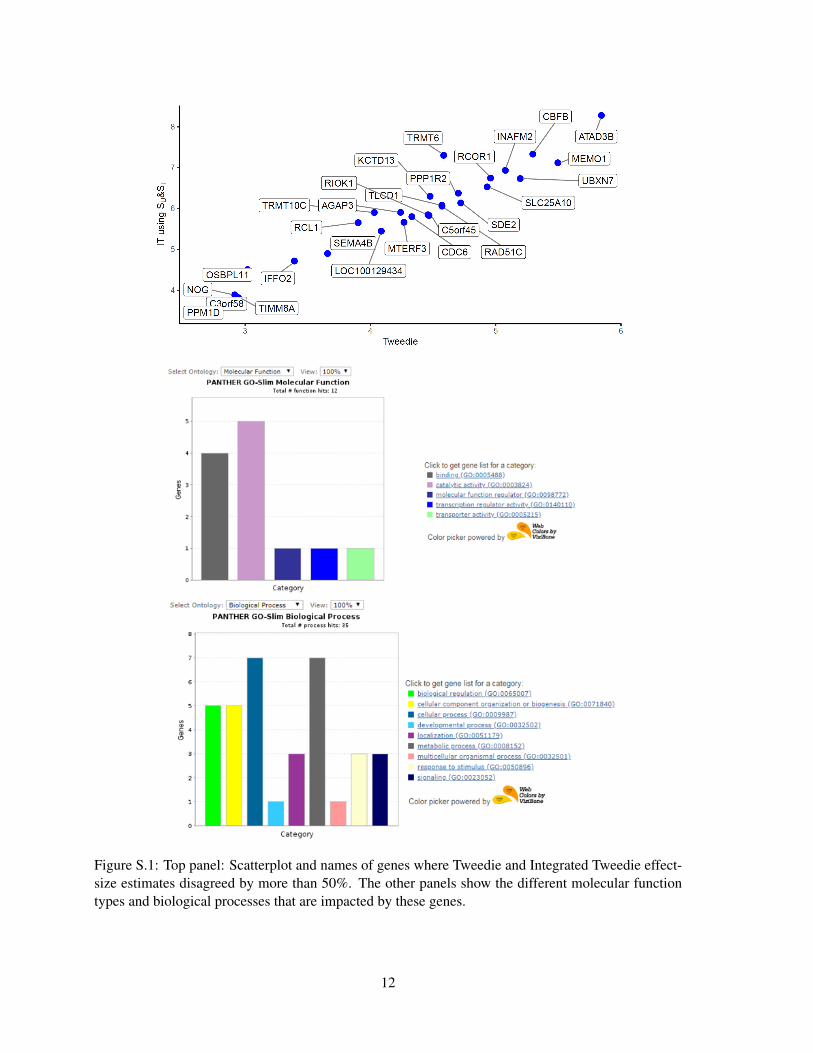
Figure S.1: Top panel: Scatterplot and names of genes where Tweedie and Integrated Tweedie effect-size estimates disagreed by more than 50%. The other panels show the different molecular functiontypes and biological processes that are impacted by these genes.
12

20
40
60
80
100
120
140
NumberofStores
Figure S.2: Distribution of the 866 stores across different states in USA.
Table S.1: Correlation matrix of the monthly sales of different products.
Products (1) (2) (3) (4)
(1) Beer 1.00(2) Milk 0.33 1.00(3) Deod 0.16 0.63 1.00(4) Hotdog 0.84 0.38 0.19 1.00
Table S.2: Monthwise % gains for monthly beer sales prediction over the naive unshrunken estimator.
July August September October November December Average
James-Stein 9.7 2.4 10.8 -2.7 -16.2 -3.7 5.7
Tweedie 7.5 7.5 9.6 -7.2 -22.6 -2.8 4
IT -Milk 11.7 5.2 9.4 -7.4 -8.8 -8.2 6
IT -Deo 11.3 5.1 10.7 -10.6 -13.7 3.7 7.1
IT -Hotdog 12.4 2.6 11.9 -3.2 -13.2 -6.5 6.8
IT-M&D 10.7 5.9 9.8 -7.4 -8.7 -7 6.1
IT-M&H 10.3 5.7 10.8 -4.3 -10.3 -4.8 6.6
IT-D&H 11.7 6.8 11 -8.2 -9.1 -0.6 7.5
IT-M&D&H 11.2 6.8 10.9 -8.1 -7.2 1.8 7.7
13
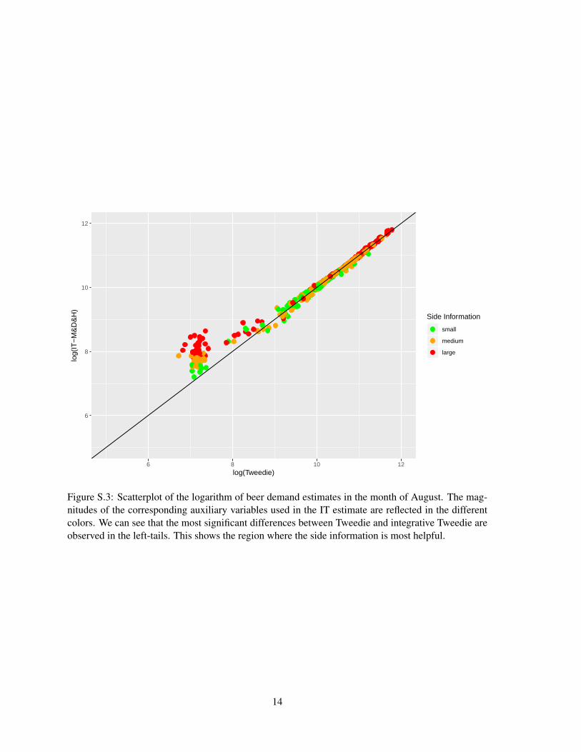
6
8
10
12
6 8 10 12log(Tweedie)
log(
IT−
M&
D&
H)
Side Information
small
medium
large
Figure S.3: Scatterplot of the logarithm of beer demand estimates in the month of August. The mag-nitudes of the corresponding auxiliary variables used in the IT estimate are reflected in the differentcolors. We can see that the most significant differences between Tweedie and integrative Tweedie areobserved in the left-tails. This shows the region where the side information is most helpful.
14

References
Bart J Bronnenberg, Michael W Kruger, and Carl F Mela. Database paperthe iri marketing data set.
Marketing science, 27(4):745–748, 2008.
Lawrence D Brown. Admissible estimators, recurrent diffusions, and insoluble boundary value prob-
lems. The Annals of Mathematical Statistics, 42(3):855–903, 1971.
Iain M Johnstone. Gaussian estimation: Sequence and wavelet models. Manuscript, December, 2011.
Huaiyu Mi, Anushya Muruganujan, and Paul D Thomas. Panther in 2013: modeling the evolution
of gene function, and other gene attributes, in the context of phylogenetic trees. Nucleic acids
research, 41(D1):D377–D386, 2012.
Nandini Sen, Phillip Sung, Arjun Panda, and Ann M Arvin. Distinctive roles for type i and type ii
interferons and interferon regulatory factors in the host cell defense against varicella-zoster virus.
Journal of virology, 92(21):e01151–18, 2018.
15


![GENERAL EMPIRICAL BAYES AW VELET METHODS ...[j] are the Bayes rules when the priors are taken to be the unknown empirical distributions of {θk,k∈[j]}. Consider the estimation of](https://img.pdfslide.net/doc/110x75/60ef897c2953690e6f7bb96f/general-empirical-bayes-aw-velet-methods-j-are-the-bayes-rules-when-the-priors.jpg)