Embed Size (px)
Citation preview
Flexible Empirical Bayes Estimation For Wavelets
By Merlise Clyde and Edward I. George 1
Summary
Wavelet shrinkage estimation is an increasingly popular method for signal denoising and compression.
Although Bayes estimators can provide excellent mean squared error (MSE) properties, selection of an
effective prior is a difficult task. To address this problem, we propose Empirical Bayes (EB) prior selection
methods for various error distributions including the normal and the heavier tailed Student t distributions.
Under such EB prior distributions, we obtain threshold shrinkage estimators based on model selection, and
multiple shrinkage estimators based on model averaging. These EB estimators are seen to be computationally
competitive with standard classical thresholding methods, and to be robust to outliers in both the data and
wavelet domains. Simulated and real examples are used to illustrate the flexibility and improved MSE
performance of these methods in a wide variety of settings.
Keywords: BAYESIAN MODEL AVERAGING; EM; HIERARCHICAL MODELS; MODEL SELECTION;
MULTIPLE SHRINKAGE; OUTLIERS; ORTHOGONAL REGRESSION; ROBUSTNESS; THRESHOLD-
ING.
1 Introduction
Wavelets are families of orthonormal basis functions that provide efficient representations for wide classes
of functions, representations that are increasingly useful for signal denoising and compression. Towards this
end and motivated by frequentist considerations, Donoho and Johnstone (1994, 1995) proposed a variety of
wavelet shrinkage procedures for estimating a function observed with normal error. For this setup, recent
papers such as Abramovich et al. (1998), Chipman et al. (1997) and Clyde et al. (1998) have proposed
Bayesian shrinkage estimators that, for a variety of functions, yield improved performance over the earlier
shrinkage methods. Although such improvements are available over broad prior classes, selection of the most
effective prior can be especially difficult when little is known about the unknown function.
In this paper, we propose Empirical Bayes (EB) methods to resolve the prior selection problem for
Bayesian estimation of wavelet coefficients. We develop these methods not only for the conventional nor-1Merlise Clyde is Assistant Professor of Statistics, Institute of Statistics and Decision Sciences, Duke University, Durham,
NC, 27708-0251, [email protected]. Edward I. George hold the Ed and Molly Smith Chair and is Professor of Statistics,
Department of MSIS, University of Texas, Austin, TX 78712-1175, [email protected]. All correspondence should be
addressed to Prof. Clyde. This work was supported by NSF grants DMS-96.26135, DMS-97.33013, and DMS-98.03756, and
Texas ARP grants 003658.130 and 003658.452.

mal error model, but also for heavier tailed error models such as Student t distributions that can better
accommodate extreme values and outliers. To handle these different error distributions, we begin with a
hierarchical Bayesian wavelet model that uses a scale mixture of normals for the error distribution (section
2). We then propose EB methods that identify EB priors by using the data to estimate the hyperparameters
and the error variance of this hierarchical model (section 3). Using these EB priors, we obtain threshold
estimators based on model selection, and multiple shrinkage estimators based on model averaging. These
EB procedures not only bypass the difficulty of specifying the hyperparameters in the prior distributions,
but are also competitive with other shrinkage methods on computational grounds. These new EB estimators
are seen to offer improved performance over previous methods in simulation studies (section 4), and are
illustrated on real data (section 5).
2 Statistical Model
Suppose Y = (Y1, . . . , Yn)′ are n equally spaced noisy observations of an unknown function f = (f1, f2, . . . , fn)′
of interest, where n is a power of 2. Let f = Wβ be an orthogonal wavelet decomposition of f , where W
is an n × n orthonormal matrix, and β is the n × 1 vector of wavelet coefficients for f . Let D = W ′Y be
the discrete wavelet transform (DWT) of Y , so that D is the n× 1 vector of empirical or observed wavelet
coefficients. For this setup, we assume the model for the data in the wavelet domain is
Djk = βjk + εjk (1)
where εjk represents an additive error term. The doubly indexed subscripts reflect the multi-resolution
nature of the wavelet decomposition; j indexes scales or levels of resolution, and k indexes locations.
A standard assumption is that the εjk are independent and normally distributed with mean zero and
variance σ2. While reasonable in many cases, extreme values and potential outliers may be more realistically
modeled by heavy tailed error distributions. To extend the error distribution beyond the standard normal
model, we replace it by a scale mixture of normals
εjk | λjk ∼ N(0, σ2/λjk) (2)
λjk ∼ h (3)
where the εjk ’s are conditionally independent, the λjk ’s are independent, and h() is a scale mixing distribution
on (0,∞). Scale mixtures of normals have been widely used in robustness studies and in outlier analysis
(Andrews and Mallows 1974, West 1984, 1987, O’Hagan 1979, 1988) and include as special cases the normal,
2

Laplace, exponential power, and Student t distributions. The normal model is obtained when λjk ≡ 1,
whereas independent errors with the tν distribution (the Student t distribution with ν degrees of freedom)
are obtained when h is a Gamma distribution,
λjk ∼ Gamma(ν/2, 2/ν) (4)
with mean 1. For notational convenience, we shall use ph(x; 0, σ) to stand for the marginal density of X
when X | λ ∼ N(0, σ2/λ) and λ ∼ h.
For nondegenerate h, independent scale mixtures of normal errors in the wavelet domain corresponds to
a scale mixture of normal errors in the data domain, though a different mixture. To see this, note that given
Λ, the diagonal matrix with diagonal terms λjk , the data domain errors are normal with covariance matrix
σ2WΛ−1W ′. Mixing over Λ yields a different scale mixture with uncorrelated but typically dependent errors.
(The unconditional covariance matrix, σ2WEh(Λ−1)W ′, is proportional to the identity matrix as the λjk
are independent and identically distributed.) In particular, if the wavelet domain errors have independent
tν distributions, then the data domain errors will be linear combinations of those tν random variables.
Although specification of independent tν distributions in the data domain may seem simpler than using
other heavy tailed error distributions, exact calculations in the wavelet domain become intractable and re-
quire computationally intensive methods. Furthermore, if the only available information about the process
is that the errors appear to be uncorrelated with a heavy tailed distribution (in either domain), then ap-
proximating the error distribution in the wavelet domain with independent tν distributions, perhaps with
level dependent ν, seems reasonable and is more appropriate than the standard normal model. At the very
least, this model provides a useful approximation which, as we show, yields computationally tractable EB
estimators for non-normal error distributions that are robust to outliers.
2.1 Hierarchical Model
The cornerstone of our Bayesian approach is an extension of the hierarchical normal mixture prior used by
(Clyde et al. 1998). Based on the natural multilevel grouping of the wavelet coefficients, this distribution
for the βjk ’s at level j is
βjk | λ∗jk , γjk ∼ N(0, σ2cjγjk/λ∗jk) (5)
λ∗jk ∼ h∗ (6)
γjk ∼ Bernoulli(ωj) (7)
3
where the βjk ’s are conditionally independent, the λ∗jk ’s and γjk’s are independent, and h∗() is a scale mixing
distribution on (0,∞). We also assume that the βjk’s and the εjk’s are conditionally independent given the
λ∗jk ’s and the λjk ’s.
When the indicator variable γjk = 0, the wavelet coefficient βjk = 0; when γjk = 1, βjk is conditionally
normal with a variance σ2cj/λ∗jk . There are two fixed hyperparameters at each level: the expected fraction
ωj of non-zero wavelet coefficients at level j, and a fixed scaling factor cj > 0 for these non-zero coefficients.
As with the error distribution, the introduction of random scale coefficients λ∗jk ’s allows for a heavy-tailed
distribution of the non-zero βjk ’s. As will be seen in the next section, the effect of the choice of h∗ on
posterior probabilities is strongly influenced by the choice of h for the error distribution.
The final specification issue concerns the dependence between the λ∗jk ’s and the λjk ’s. Because we do
not expect a relationship between the signal and noise components, the most reasonable choice would be to
specify these as independent, in which case the βjk ’s and the εjk ’s would be unconditionally independent.
However, as will be seen, the EB calculations under this independent λ specification become analytically
intractable and must be carried out numerically.
To substantially ease the computational burden, it may be useful to consider the alternative specification
obtained by forcing λ∗jk = λjk but maintaining the independence of the λjk ’s. Under this common λ
specification, each βjk and εjk pair are still uncorrelated (because of their conditional independence), but
become unconditionally dependent through λjk . As is illustrated in Figure 1 in the next section, this
dependence appears to have only a mild effect on posterior quantities of interest. Because the resulting
posterior calculations are faster than the fully independent (λjk , λ∗jk) model and yield predictions that
compare favorably with competing methods, this common λ specification is at least a useful approximation
to the full independence specification.
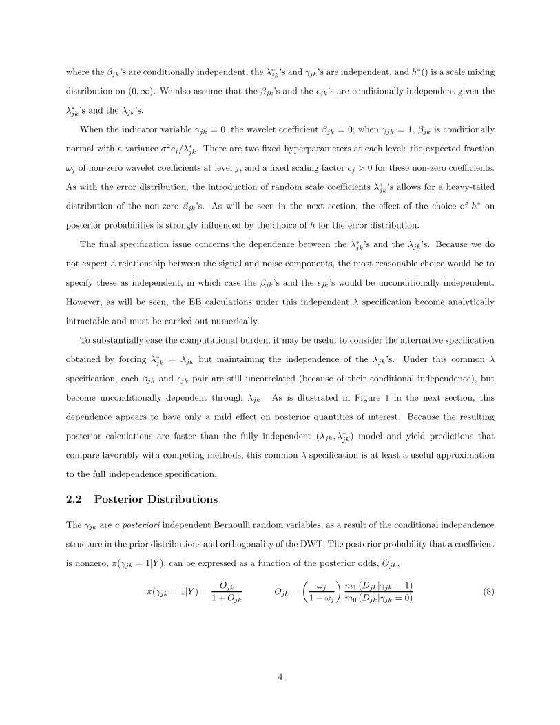
2.2 Posterior Distributions
The γjk are a posteriori independent Bernoulli random variables, as a result of the conditional independence
structure in the prior distributions and orthogonality of the DWT. The posterior probability that a coefficient
is nonzero, π(γjk = 1|Y ), can be expressed as a function of the posterior odds, Ojk ,
π(γjk = 1|Y ) =Ojk
1 + OjkOjk =
(
ωj
1− ωj
)
m1 (Djk |γjk = 1)
m0 (Djk |γjk = 0)(8)
4
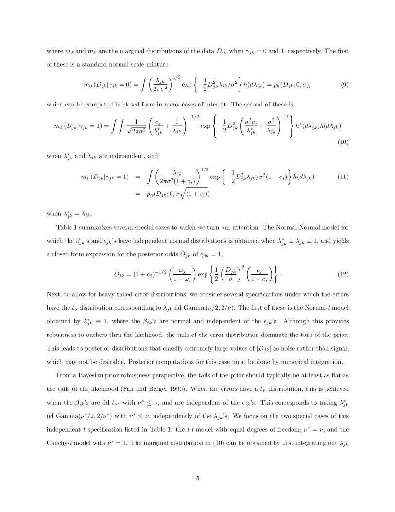
where m0 and m1 are the marginal distributions of the data Djk when γjk = 0 and 1, respectively. The first
of these is a standard normal scale mixture
m0 (Djk |γjk = 0) =
∫(
λjk
2πσ2
)1/2
exp
{
−1
2D2
jkλjk/σ2
}
h(dλjk) = ph(Djk ; 0, σ), (9)
which can be computed in closed form in many cases of interest. The second of these is
m1 (Djk|γjk = 1) =
∫ ∫
1√2πσ2
(
cj
λ∗jk
+1
λjk
)
−1/2
exp
−1
2D2
jk
(
σ2cj
λ∗jk
+σ2
λjk
)
−1
h∗(dλ∗jk)h(dλjk)
(10)
when λ∗jk and λjk are independent, and
m1 (Djk |γjk = 1) =
∫(
λjk
2πσ2(1 + cj)
)1/2
exp
{
−1
2D2
jkλjk/σ2(1 + cj)
}
h(dλjk) (11)
= ph(Djk; 0, σ√
(1 + cj))
when λ∗jk = λjk .
Table 1 summarizes several special cases to which we turn our attention. The Normal-Normal model for
which the βjk ’s and εjk’s have independent normal distributions is obtained when λ∗jk ≡ λjk ≡ 1, and yields
a closed form expression for the posterior odds Ojk of γjk = 1,
Ojk = (1 + cj)−1/2
(
ωj
1− ωj
)
exp
{
1
2
(
Djk
σ
)2(cj
1 + cj
)
}
. (12)
Next, to allow for heavy tailed error distributions, we consider several specifications under which the errors
have the tν distribution corresponding to λjk iid Gamma(ν/2, 2/ν). The first of these is the Normal-t model
obtained by λ∗jk ≡ 1, where the βjk ’s are normal and independent of the εjk ’s. Although this provides
robustness to outliers thru the likelihood, the tails of the error distribution dominate the tails of the prior.
This leads to posterior distributions that classify extremely large values of |Djk| as noise rather than signal,
which may not be desirable. Posterior computations for this case must be done by numerical integration.
From a Bayesian prior robustness perspective, the tails of the prior should typically be at least as flat as
the tails of the likelihood (Fan and Berger 1990). When the errors have a tν distribution, this is achieved
when the βjk ’s are iid tν∗ with ν∗ ≤ ν, and are independent of the εjk’s. This corresponds to taking λ∗jk
iid Gamma(ν∗/2, 2/ν∗) with ν∗ ≤ ν, independently of the λjk ’s. We focus on the two special cases of this
independent t specification listed in Table 1: the t-t model with equal degrees of freedom, ν∗ = ν, and the
Cauchy-t model with ν∗ = 1. The marginal distribution in (10) can be obtained by first integrating out λjk
5
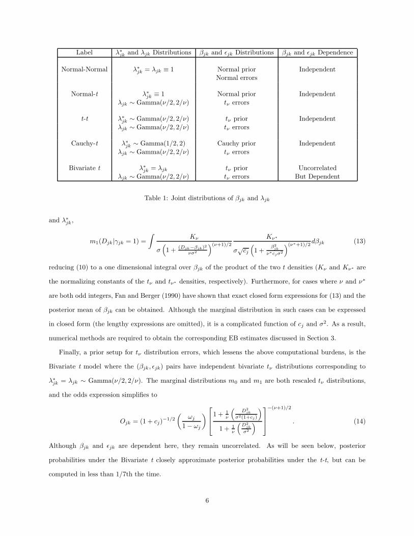
Label λ∗jk and λjk Distributions βjk and εjk Distributions βjk and εjk Dependence
Normal-Normal λ∗jk = λjk ≡ 1 Normal prior Independent
Normal errors
Normal-t λ∗jk ≡ 1 Normal prior Independent
λjk ∼ Gamma(ν/2, 2/ν) tν errors
t-t λ∗jk ∼ Gamma(ν/2, 2/ν) tν prior Independent
λjk ∼ Gamma(ν/2, 2/ν) tν errors
Cauchy-t λ∗jk ∼ Gamma(1/2, 2) Cauchy prior Independent
λjk ∼ Gamma(ν/2, 2/ν) tν errors
Bivariate t λ∗jk = λjk tν prior Uncorrelated
λjk ∼ Gamma(ν/2, 2/ν) tν errors But Dependent
Table 1: Joint distributions of βjk and λjk
and λ∗jk ,
m1(Djk |γjk = 1) =
∫
Kν
σ(
1 +(Djk−βjk)2
νσ2
)(ν+1)/2
Kν∗
σ√
cj
(
1 +β2
jk
ν∗cjσ2
)(ν∗+1)/2dβjk (13)
reducing (10) to a one dimensional integral over βjk of the product of the two t densities (Kν and Kν∗ are
the normalizing constants of the tν and tν∗ densities, respectively). Furthermore, for cases where ν and ν∗
are both odd integers, Fan and Berger (1990) have shown that exact closed form expressions for (13) and the
posterior mean of βjk can be obtained. Although the marginal distribution in such cases can be expressed
in closed form (the lengthy expressions are omitted), it is a complicated function of cj and σ2. As a result,
numerical methods are required to obtain the corresponding EB estimates discussed in Section 3.
Finally, a prior setup for tν distribution errors, which lessens the above computational burdens, is the
Bivariate t model where the (βjk , εjk) pairs have independent bivariate tν distributions corresponding to
λ∗jk = λjk ∼ Gamma(ν/2, 2/ν). The marginal distributions m0 and m1 are both rescaled tν distributions,
and the odds expression simplifies to
Ojk = (1 + cj)−1/2
(
ωj
1− ωj
)
1 + 1ν
(
D2jk
σ2(1+cj)
)
1 + 1ν
(
D2jk
σ2
)
−(ν+1)/2
. (14)
Although βjk and εjk are dependent here, they remain uncorrelated. As will be seen below, posterior
probabilities under the Bivariate t closely approximate posterior probabilities under the t-t, but can be
computed in less than 1/7th the time.
6
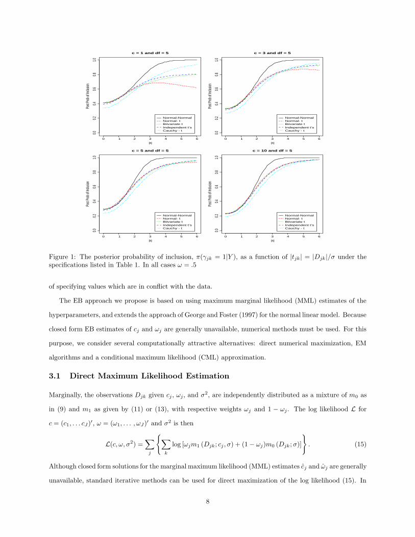
Figure 1 shows the posterior probability π(γjk = 1|Y ) as a function of |tjk | = |Djk|/σ for various choices
of cj under each of the priors listed in Table 1 for ν = 5. (Numerical integration was required to compute
the curves for the Normal-t model). Under the Normal-Normal model when cj > 0, π(γjk = 1|Y ) increases
rapidly in |tjk | to 1, thus treating extreme values as signal. In sharp contrast, under the Normal-t model,
π(γjk = 1|Y ) eventually decreases in |tjk |, causing it to treat extreme values as noise. This occurs because
the tails of the tν distribution eventually dominate the normal prior. This behavior, which is more evident
when cj is small, is undesirable for functions that have a few very large coefficients at the finest level because
the Normal-t model would tend to treat them as outliers.
The Cauchy-t curve corresponds to an independent t specification with a Cauchy prior (ν∗ = 1) and a
t5 error distribution. The Cauchy prior is the easiest of the independent t priors to handle computationally,
and has desirable robustness properties. Like the Normal-Normal, π(γjk = 1|Y ) under the Cauchy-t even-
tually approaches 1 for large |Djk|. However, it does so more slowly, exhibiting greater uncertainty that an
observation represents signal.
The π(γjk = 1|Y ) curves for both the Bivariate t and t-t model (with ν∗ = ν = 5) are very similar,
especially for cj large. Providing a compromise between the Normal-Normal and the Normal-t models, both
add robustness while avoiding the Normal-t non-monotonicity phenomenon. For the Bivariate t model, the
posterior odds Ojk has a limit of (ωj/(1+ωj))(1+ cj)νj/2, as |tjk| goes to infinity. For large cj , this behaves
effectively like the normal model. However, compared to both the Normal-Normal and the Cauchy-t models,
for small cj (where it is difficult to distinguish between signal and noise), there is more uncertainty about
whether a coefficient is nonzero, which does not disappear for large |Djk|. Because of the availability of simple
closed form posterior expressions, the Bivariate t model can be seen as an attractive approximation to the
t-t model, providing a reasonable compromise between robust estimation and computational ease. Because
of the similarity of the Bivariate t and the t-t, we will proceed to focus our attention on the Normal-Normal,
Bivariate t and the Cauchy-t models.
3 Empirical Bayes Methods
Implementation of the Bayes hierarchical model (5)-(7), with fixed hyperparameter values requires the speci-
fication of cj and ωj at each level j of the wavelet decomposition. Unfortunately, meaningful pre-specification
of these is difficult at best. Although one’s prior beliefs might reflect an ordering of the cj and ωj by level,
it is difficult to subjectively elicit additional information. A fully automatic Empirical Bayes (EB) approach
that estimates cj , ωj and σ2 from the data is appealing because it avoids this difficulty and the possibility
7
0 1 2 3 4 5 6
0.00.2
0.40.6
0.81.0
|t|
Post
Prob
of In
clusio
n
Normal-NormalNormal- tBiivariate tIndependent t’sCauchy - t
c = 1 and df = 5
0 1 2 3 4 5 6
0.00.2
0.40.6
0.81.0
|t|
Post
Prob
of In
clusio
n
Normal-NormalNormal- tBiivariate tIndependent t’sCauchy - t
c = 3 and df = 5
0 1 2 3 4 5 6
0.00.2
0.40.6
0.81.0
|t|
Post
Prob
of In
clusio
n
Normal-NormalNormal- tBiivariate tIndependent t’sCauchy - t
c = 5 and df = 5
0 1 2 3 4 5 6
0.00.2
0.40.6
0.81.0
|t|
Post
Prob
of In
clusio
nNormal-NormalNormal- tBiivariate tIndependent t’sCauchy - t
c = 10 and df = 5
Figure 1: The posterior probability of inclusion, π(γjk = 1|Y ), as a function of |tjk| = |Djk |/σ under thespecifications listed in Table 1. In all cases ω = .5
of specifying values which are in conflict with the data.
The EB approach we propose is based on using maximum marginal likelihood (MML) estimates of the
hyperparameters, and extends the approach of George and Foster (1997) for the normal linear model. Because
closed form EB estimates of cj and ωj are generally unavailable, numerical methods must be used. For this
purpose, we consider several computationally attractive alternatives: direct numerical maximization, EM
algorithms and a conditional maximum likelihood (CML) approximation.
3.1 Direct Maximum Likelihood Estimation
Marginally, the observations Djk given cj , ωj , and σ2, are independently distributed as a mixture of m0 as
in (9) and m1 as given by (11) or (13), with respective weights ωj and 1 − ωj . The log likelihood L for
c = (c1, . . . cJ)′, ω = (ω1, . . . , ωJ)′ and σ2 is then
L(c, ω, σ2) =∑
j
{
∑
k
log [ωjm1 (Djk; cj , σ) + (1− ωj)m0 (Djk ; σ)]
}
. (15)
Although closed form solutions for the marginal maximum likelihood (MML) estimates cj and ωj are generally
unavailable, standard iterative methods can be used for direct maximization of the log likelihood (15). In
8
particular, we have found nonlinear Gauss-Seidel iteration (Thisted 1988, pp 187-188) to work well. This
entails iterating between finding the maximizing cj given (ωj , σ2), the maximizing ωj given (cj , σ
2) for each
j, and the maximizing σ2 given (c1, ω1), . . . , (cJ , ωJ). As the Hessian of the log likelihood is in general not
positive definite for all values of cj , ωj , and σ2, convergence may only be to a local mode. However, we have
achieved reasonable success using the MAD estimate σ = Median(|D1k|)/0.6745 (Donoho et al. 1995) as an
initial value for σ, and ωj equal to the number of observed wavelet coefficients that exceed√
2 log n σ based
on hard thresholding.
3.2 Maximum Likelihood Estimation using the EM Algorithm
For the Normal-Normal model with a fixed value for σ2, Johnstone and Silverman (1998) have recently
proposed an EM algorithm based on a metric inequality. To implement a more general EM algorithm here,
we consider the augmented log likelihood given D and latent or “missing” variables λ and γ. This leads to
an alternative method for maximizing the marginal likelihood in (15). Unless, otherwise noted, we shall now
restrict attention to common λ models such as the Normal-Normal and the Bivariate t where λ∗
jk = λjk ,
which leads to closed form iterative solutions for the parameters.
Let τ−1j = (1 + cj)σ
2, where τj corresponds to the unknown precision parameter for the data, Djk , given
γjk = 1 and let φ = 1/σ2, the precision when γjk = 0. The log likelihood for τ = (τ1, . . . , τJ )′, ω and φ
based on the “augmented” or “completed” data, X = (D, λ, γ), is
L(ω, τ, φ|D, λ, γ) =∑
j
[
nj log(1− ωj) + log
(
ωj
1− ωj
)
∑
k
γjk
]
+1
2
∑
j
[
log(τj)∑
k
γjk − τj
∑
k
D2jkλjkγjk
]
+1
2log(φ)
∑
jk
(1− γjk)− 1
2φ∑
j,k
D2jkλjk(1− γjk)
+∑
jk
log (h(λjk)) (16)
and belongs to a regular exponential family of the form a(θ)′b(X) + c(θ) + d(X) where θ = (ω, τ, φ), a(θ)
is the 2J + 1 dimensional vector of natural parameters, and b(X) is the 2J + 1 vector of sufficient statistics
with components (∑
k γjk,∑
k D2jkλjkγjk) for j = 1, . . . J and
∑
jk D2jkλjk(1− γjk).
The E-step of the EM algorithm consists of computing the expectations of the sufficient statistics with
respect to the distribution of (λ, γ) given D, c, and ω. The posterior mean of γjk is
E(γjk |D) = γ(i)jk =
O(i)jk
1 + O(i)jk
9
where O(i)jk is the posterior odds (8) evaluated using the current estimates c
(i)j and ω
(i)j . For the Bivariate t
model, where λjk ∼ Gamma(νj/2, 2/νj), the posterior distribution of λjk given γjk is Gamma, with
E(λjkγjk|D) =νj + 1
νj + D2jk τ
(i)j
γ(i)jk = [λjk γjk ](i)
E(λjk(1− γjk)|D) =νj + 1
νj + D2jkφ(i)
(1− γ(i)jk ) = [λjk(1− γjk)](i).
The M-step consists of maximizing the augmented likelihood with the latent data now replaced by their
posterior expected values, resulting in
σ2(i+1)
=
∑
jk D2jk[λjk(1− γjk)](i)
n−∑jk γ(i)jk
(17)
ω(i+1)j =
∑
k γ(i)jk
nj(18)
c(i+1)j = max
(
0,
∑
k D2jk [λjk γjk ](i)
σ2(i+1)∑
k γ(i)jk
− 1
)
. (19)
The EM algorithm for the Normal-Normal model is obtained by simply setting λjk ≡ 1 in the above.
If the parameter estimates are in the interior of the parameter space, the solutions above are the unique
solutions (conditional on the values of latent data) because the complete data belong to a regular exponential
family. The E and M steps are repeated until the estimates converge, and yield a stationary point of the
marginal likelihood (15). However, as in the case of direct maximization of the marginal likelihood using
Gauss-Seidel or other methods, the EM algorithm may converge to a local mode. Because the convergence
rate of the standard EM algorithm is linear (Dempster, Laird, and Rubin 1977), the direct maximization
methods described above may result in faster convergence. However, the iterative solutions are available in
closed form for the common scale λjk model and provide some insight into the problem and connections to the
CML estimates of George and Foster (1997). The M-step estimates of σ2 and wj have natural interpretations;
the estimate of σ2 is the ratio of the posterior expected error sum of squares to the posterior expected df,
and the estimate of wj is the posterior expected fraction of nonzero coefficients.
While it is not necessary to introduce λjk as a latent variable, this does permit closed form iterative
expressions for the hyperparameter estimates of the Bivariate t model. For models where the complete data
are not from a regular exponential family, such as in the Cauchy-t model, numerical optimization is required
to carry out the M-step for cj and σ2, although ωj has the same form as in (18). In practice, we have noticed
very little difference between MLEs using the EM algorithm or the direct maximization approach for the
Normal-Normal, Bivariate t or Cauchy-t models.
10
3.3 Conditional Likelihood Approximations
For the Normal-Normal model, the conditional maximum likelihood (CML) approach of George and Foster
(1997) provides a fast alternative to direct maximization and EM, and can be viewed as taking the complete
data likelihood (16) and evaluating it at the mode for γ, rather than using the posterior mean, as in the
EM algorithm. Let qj =∑
k γjk denote the the number of nonzero wavelet coefficients at level j. For fixed
j, let D2j(k) denote the sorted values (in decreasing order) of (Djk/σ)2, where σ2 corresponds to the MAD
estimate of σ2. The most likely model with qj nonzero components at level j, γ(qj) has elements γj(k) = 1
if k ≤ qj , and 0 otherwise.
For each value of qj , the values of cj and ωj that maximize the conditional log likelihood are
ωj(qj) =
∑
k γj(k)(qj)
nj= qj/nj cj(qj) = max
{
0,
∑
k D2j(k)γj(k)(qj)
∑
k γj(k)(qj)σ2− 1
}
. (20)
The CML estimators have the same form as the EM MML estimators, and are the same when the posterior
distribution for γjk is degenerate at 1 or 0, where we have perfect classification of the observation into noise
or signal. For large values of cj , there is often very good separation of signal and noise, resulting in little
bias of the CML estimators.
The difference between the MML and the CML estimates will be the most extreme when the posterior
mean of γjk is 0.5 and when cj is small. The simulation studies described later suggest, however, that the EB
estimators using the conditional estimates have better MSE performance than earlier shrinkage estimators.
Although this approach does not readily extend to the case of t errors without further approximations, the
Normal-Normal model solutions can be used as starting values for iterative methods such as the Gauss-Seidel
or EM algorithms.
3.4 Empirical Bayes Estimators
We consider two types of Empirical Bayes estimators: threshold shrinkage estimators based on model se-
lection, and multiple shrinkage estimators based on model averaging. The EB estimators are obtained as
posterior means, treating the MML hyperparameter estimates as if they were fixed in advance. The βjks
under the common λ model are a posteriori conditionally independent,
p(βjk |γjk , λjk , Y ) ∼ N
(
γjkcj
1 + cjDjk ,
γjk
λjkσ2 cj
1 + cj
)
. (21)
Expressions for the posterior mean of βjk given γjk = 1 under the Cauchy-t model can be obtained from
equations in Fan and Berger (1990). Unless noted otherwise, all results below hold for the Cauchy-t model,
with (cj/(1 + cj)) Djk replaced by E[βjk|γjk = 1, Y ] computed under the Cauchy-t model.
11
Threshold Shrinkage Estimators
Thresholded shrinkage estimators are obtained as posterior means conditionally on the highest posterior
probability model or γ = (γ11, . . . , γJK). (As in the variable selection context, a “model” can be identified
with γ). As a consequence of the conditional independence structure, the posterior probability of γ is of the
form
p(γ|D) =∏
jk
π(γjk = 1|Djk)γjk (1− π(γjk = 1|Djk))(1−γjk), (22)
a product of independent Bernoulli probabilities. Because of the product structure, the highest posterior
probability model, γ = (γ11, . . . , γJK), is obtained by setting γjk = 1 if π(γjk = 1|Djk) ≥ 0.5 and γjk = 0
otherwise. The posterior mean under γ for the common λ model is then
E(βjk |γ, Y ) = γjkcj
1 + cjDjk. (23)
This threshold shrinkage estimator thresholds the data by setting βjk = 0 whenever γjk = 0, and then
shrinks the remaining coefficients. This is useful for compression problems where dimension reduction and
elimination of negligible coefficients is important. Because the inverse DWT (IDWT) is linear, the posterior
mean of f under model γ is obtained by applying the IDWT to the posterior mean of β under model γ.
Multiple Shrinkage Estimators
Instead of conditioning on a single model as above, an estimator of βjk which incorporates uncertainty about
γjk , is the unconditional posterior mean
E(βjk |Y ) = π(γjk = 1|Y )cj
1 + cjDjk. (24)
Note that π(γjk = 1|Y ) = π(γjk = 1|Djk) is given by (8), where the marginals m0 and m1 are based on the
EB hyperparameter estimates cj and ωj . For specifications such as the Normal-Normal and the Bivariate
t, the resulting closed form expressions for π(γjk = 1|Y ) and the EB multiple shrinkage estimators can be
computed quickly once we have the hyperparameter estimates. In contrast, the multiple shrinkage estimator
for the Cauchy-t takes approximately 30 times longer (not including the extra time necessary to obtain the
hyperparameter estimates) for n = 1024. The posterior mean of f is obtained by applying the IDWT to the
multiple shrinkage estimator of β.
The estimator (24) is a multiple shrinkage estimator (George 1986, Clyde et al. 1998) and corresponds to
model averaging. Because of the form of the conditional distribution (21), the usual posterior weighted sum
12
of conditional expectations reduces here to the simple form (24) that inserts π(γjk = 1|Y ) as an additional
shrinkage factor. As opposed to the threshold shrinkage estimator, which sets negligible coefficients to zero,
the multiple shrinkage estimator provides nonzero estimates for all coefficients for which π(γjk = 1|Djk) 6= 0.
For problems where threshold shrinkage rather than multiple shrinkage is desired, it is worth noting that
the threshold estimator (23) minimizes squared error loss for estimation or prediction under model selection
(J.O. Berger, personal communication). We provide a proof for the case of wavelet regression. Let fγ denote
the posterior mean for f under model γ corresponding to (23), and let f denote the unconditional posterior
mean corresponding to (24); f is the Bayes rule under squared error loss for estimation of f . The best single
model γ∗ for estimating f under posterior expected squared error loss is the model such that fγ is closest to
f , or that minimizes
(fγ − f)′(fγ − f).
Because W is orthonormal, this can be equivalently expressed in the wavelet domain by
(fγ − f)′WW ′(fγ − f) =∑
jk
(γjk − π(γjk = 1|Y ))2(E[βjk |Y, γjk = 1])2.
The last expression is minimized by the model with γ∗jk = 1 if π(γjk = 1|Y ) ≥ 0.5 and with γ∗jk = 0 if
π(γjk = 1|Y ) < 0.5, which is equivalent to the highest posterior model when the posterior distribution for γ
has the form given by (22) and is the median probability model as defined by Berger.
Although the multiple shrinkage estimator tends to outperform the threshold shrinkage estimator in
terms of squared error loss, sometimes the improvements are small. Such gains may not compensate for the
costs of including additional terms, as might occur, for example, in compression problems. We will see in
the next section that both (23) and (24) appear to offer improved frequentist risk performance over several
classical estimators.
4 Simulations
To investigate the practical potential of our EB method, we evaluated the performance of the EB estimators
under the Normal-Normal, the Bivariate t and Cauchy-t specifications, using noisy versions of the four test
functions “blocks”, “bumps”, “doppler”, “heavisine” proposed by Donoho and Johnstone (1994). In every
case, the functions were scaled so that the signal-to-noise ratio was 7, (the ratio of the standard deviation
of the function values fi to the standard deviation of the noise). We compared this performance with that
of several existing shrinkage strategies: HARD - Hard thresholding with the universal rule, SOFT - Soft
thresholding with the universal rule, and SURE - SureShrink adaptive shrinkage rule as implemented in
13
0.06
0.10
0.14
0.18
•
EBEMS
EBAMS
EBETS
EBATS
Hard
blocks
0.25
0.35
0.45 ••
EBEMS
EBAMS
EBETS
EBATS
Hard
bumps
0.10
0.20
0.30
•
•
EBEMS
EBAMS
EBETS
EBATS
Hard
doppler
0.06
0.10
0.14
••
EBEMS
EBAMS
EBETS
EBATS
Hard
heavisine
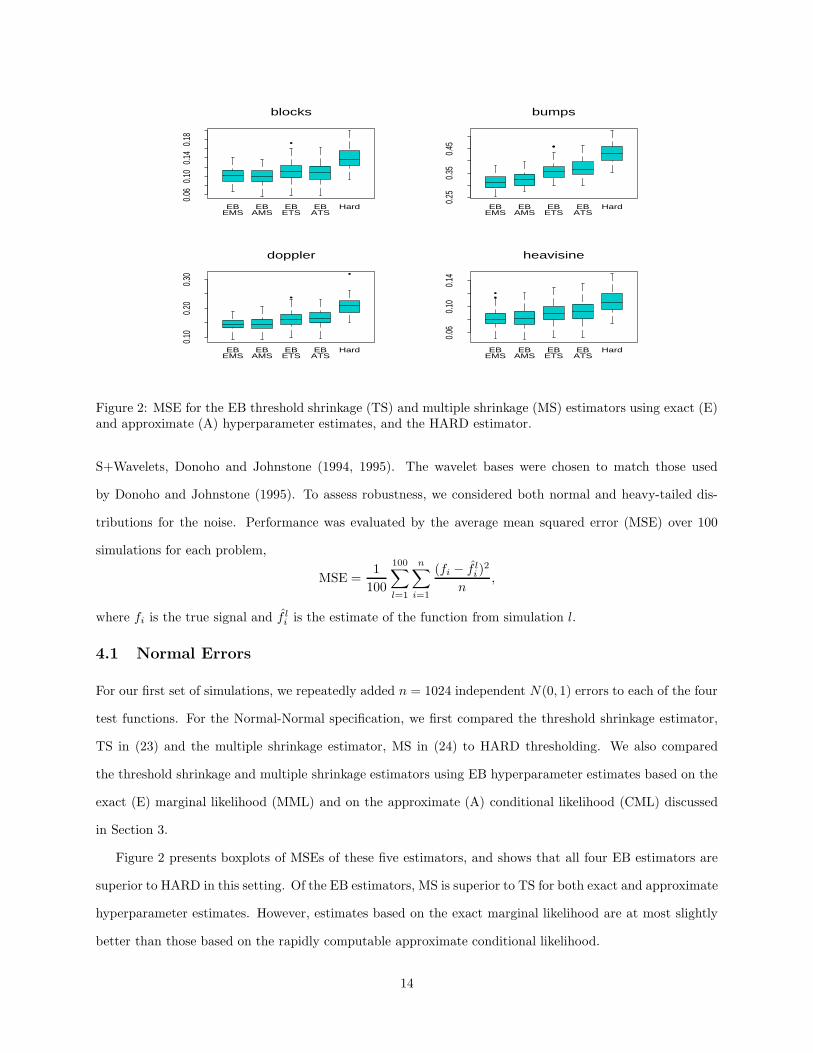
Figure 2: MSE for the EB threshold shrinkage (TS) and multiple shrinkage (MS) estimators using exact (E)and approximate (A) hyperparameter estimates, and the HARD estimator.
S+Wavelets, Donoho and Johnstone (1994, 1995). The wavelet bases were chosen to match those used
by Donoho and Johnstone (1995). To assess robustness, we considered both normal and heavy-tailed dis-
tributions for the noise. Performance was evaluated by the average mean squared error (MSE) over 100
simulations for each problem,
MSE =1
100
100∑
l=1
n∑
i=1
(fi − f li )
2
n,
where fi is the true signal and f li is the estimate of the function from simulation l.
4.1 Normal Errors
For our first set of simulations, we repeatedly added n = 1024 independent N(0, 1) errors to each of the four
test functions. For the Normal-Normal specification, we first compared the threshold shrinkage estimator,
TS in (23) and the multiple shrinkage estimator, MS in (24) to HARD thresholding. We also compared
the threshold shrinkage and multiple shrinkage estimators using EB hyperparameter estimates based on the
exact (E) marginal likelihood (MML) and on the approximate (A) conditional likelihood (CML) discussed
in Section 3.
Figure 2 presents boxplots of MSEs of these five estimators, and shows that all four EB estimators are
superior to HARD in this setting. Of the EB estimators, MS is superior to TS for both exact and approximate
hyperparameter estimates. However, estimates based on the exact marginal likelihood are at most slightly
better than those based on the rapidly computable approximate conditional likelihood.
14
0.2
0.4
0.6
••
••
EBN
EBT5
EBC5
Sure Hard Soft
blocks
0.5
1.0
1.5
• •
•
••
EBN
EBT5
EBC5
Sure Hard Soft
bumps
0.1
0.2
0.3
0.4
0.5
• • ••• •
•
EBN
EBT5
EBC5
Sure Hard Soft
doppler
0.06
0.10
0.14
0.18
•
••
•••••
EBN
EBT5
EBC5
Sure Hard Soft
heavisine
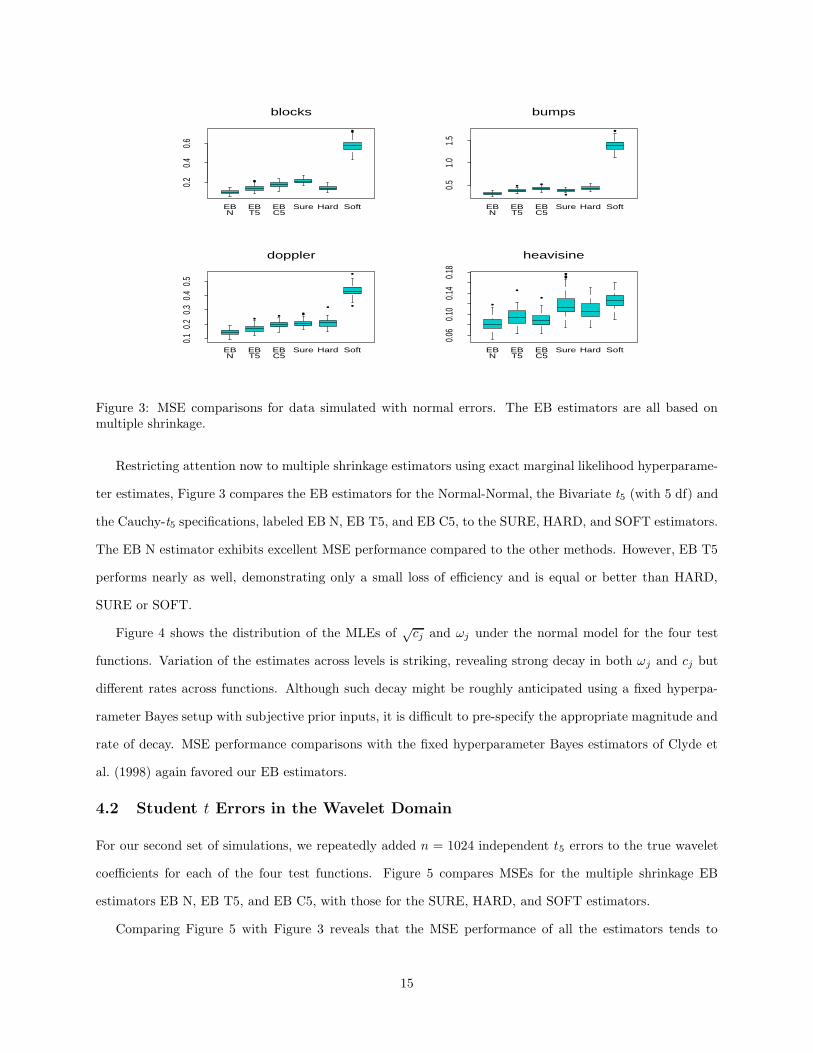
Figure 3: MSE comparisons for data simulated with normal errors. The EB estimators are all based onmultiple shrinkage.
Restricting attention now to multiple shrinkage estimators using exact marginal likelihood hyperparame-
ter estimates, Figure 3 compares the EB estimators for the Normal-Normal, the Bivariate t5 (with 5 df) and
the Cauchy-t5 specifications, labeled EB N, EB T5, and EB C5, to the SURE, HARD, and SOFT estimators.
The EB N estimator exhibits excellent MSE performance compared to the other methods. However, EB T5
performs nearly as well, demonstrating only a small loss of efficiency and is equal or better than HARD,
SURE or SOFT.
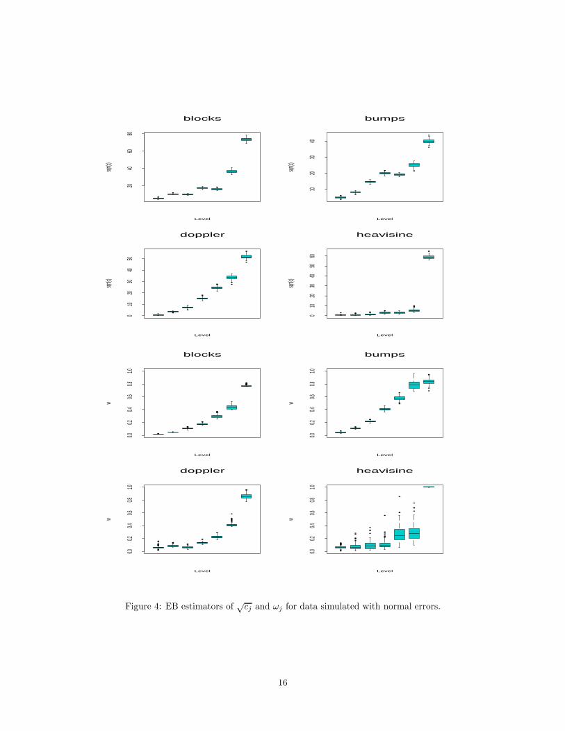
Figure 4 shows the distribution of the MLEs of√
cj and ωj under the normal model for the four test
functions. Variation of the estimates across levels is striking, revealing strong decay in both ωj and cj but
different rates across functions. Although such decay might be roughly anticipated using a fixed hyperpa-
rameter Bayes setup with subjective prior inputs, it is difficult to pre-specify the appropriate magnitude and
rate of decay. MSE performance comparisons with the fixed hyperparameter Bayes estimators of Clyde et
al. (1998) again favored our EB estimators.
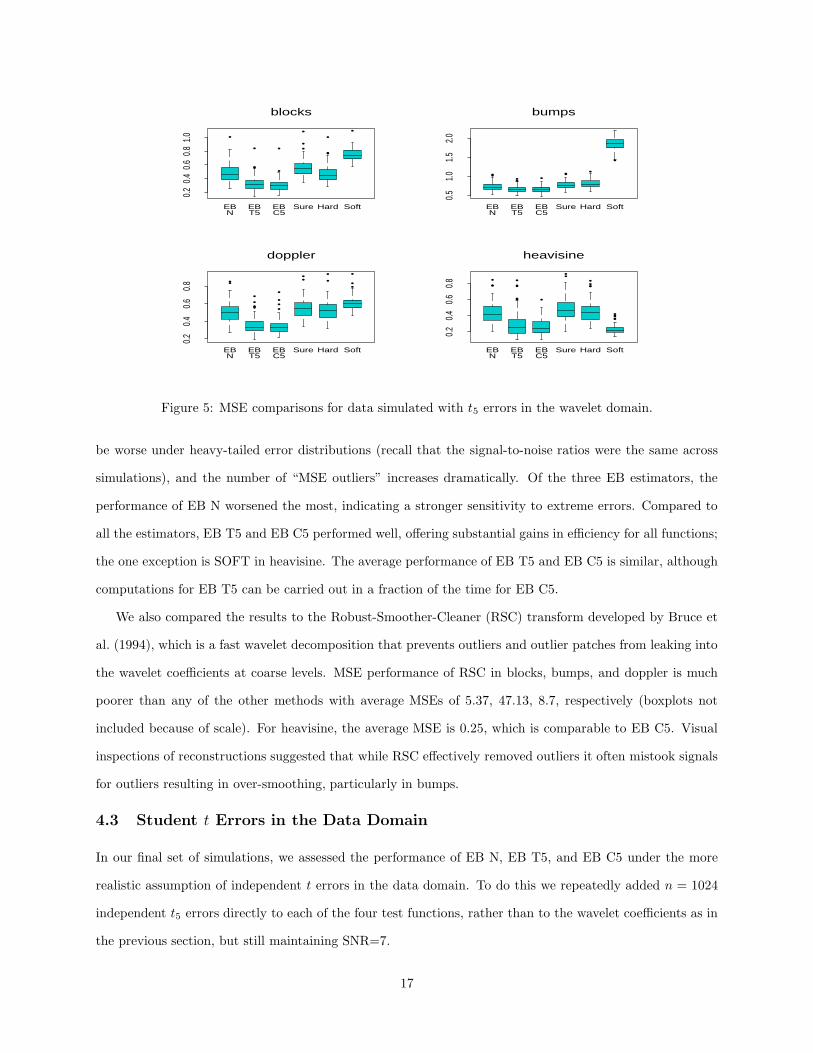
4.2 Student t Errors in the Wavelet Domain
For our second set of simulations, we repeatedly added n = 1024 independent t5 errors to the true wavelet
coefficients for each of the four test functions. Figure 5 compares MSEs for the multiple shrinkage EB
estimators EB N, EB T5, and EB C5, with those for the SURE, HARD, and SOFT estimators.
Comparing Figure 5 with Figure 3 reveals that the MSE performance of all the estimators tends to
15
2040
6080
••
•
Level
sqrt(c)
blocks
1020
3040
•• •
• •
•
•
Level
sqrt(c)
bumps
010
2030
4050
•••
••
•• ••
•
•
Level
sqrt(c)
doppler
010
2030
4050
60• •• •• •
•••
••
Level
sqrt(c)
heavisine
0.00.2
0.40.6
0.81.0
••
•••
••
•••
••••••••••••
Level
w
blocks
0.00.2
0.40.6
0.81.0
•••
••
••
•••
••
Level
w
bumps
0.00.2
0.40.6
0.81.0
•••••••••••••
••• ••••
•
•••••••
••
Level
w
doppler
0.00.2
0.40.6
0.81.0
••
••••••••
•••••• •
•••
••••••
•••
•
••••
•
Level
w
heavisine
Figure 4: EB estimators of√
cj and ωj for data simulated with normal errors.
16
0.2
0.4
0.6
0.8
1.0 •
••
•
•
• ••
•
••
••
EBN
EBT5
EBC5
Sure Hard Soft
blocks
0.5
1.0
1.5
2.0
•••• • •• •
•
EBN
EBT5
EBC5
Sure Hard Soft
bumps
0.2
0.4
0.6
0.8 ••
•••••
••••
•• ••
•••
EBN
EBT5
EBC5
Sure Hard Soft
doppler
0.2
0.4
0.6
0.8
•••
••
•••
•
••
••••
•••••
EBN
EBT5
EBC5
Sure Hard Soft
heavisine
Figure 5: MSE comparisons for data simulated with t5 errors in the wavelet domain.
be worse under heavy-tailed error distributions (recall that the signal-to-noise ratios were the same across
simulations), and the number of “MSE outliers” increases dramatically. Of the three EB estimators, the
performance of EB N worsened the most, indicating a stronger sensitivity to extreme errors. Compared to
all the estimators, EB T5 and EB C5 performed well, offering substantial gains in efficiency for all functions;
the one exception is SOFT in heavisine. The average performance of EB T5 and EB C5 is similar, although
computations for EB T5 can be carried out in a fraction of the time for EB C5.
We also compared the results to the Robust-Smoother-Cleaner (RSC) transform developed by Bruce et
al. (1994), which is a fast wavelet decomposition that prevents outliers and outlier patches from leaking into
the wavelet coefficients at coarse levels. MSE performance of RSC in blocks, bumps, and doppler is much
poorer than any of the other methods with average MSEs of 5.37, 47.13, 8.7, respectively (boxplots not
included because of scale). For heavisine, the average MSE is 0.25, which is comparable to EB C5. Visual
inspections of reconstructions suggested that while RSC effectively removed outliers it often mistook signals
for outliers resulting in over-smoothing, particularly in bumps.
4.3 Student t Errors in the Data Domain
In our final set of simulations, we assessed the performance of EB N, EB T5, and EB C5 under the more
realistic assumption of independent t errors in the data domain. To do this we repeatedly added n = 1024
independent t5 errors directly to each of the four test functions, rather than to the wavelet coefficients as in
the previous section, but still maintaining SNR=7.
17
0.2
0.4
0.6
0.8
1.0
••••
•••••
•••••
•••••
•
••••••
EBN
EBT5
EBTM
EBC5
SureHard Soft
blocks
0.5
1.0
1.5
2.0
2.5
••
••••
••••
••• ••
• •
EBN
EBT5
EBTM
EBC5
SureHard Soft
bumps
0.2
0.4
0.6
0.8
••••••
•
••
•
••
•
••
•••••
••••••
•
EBN
EBT5
EBTM
EBC5
SureHard Soft
doppler
0.1
0.2
0.3
0.4
0.5
••••
•• ••••••••
•
•••
••
EBN
EBT5
EBTM
EBC5
SureHard Soft
heavisine
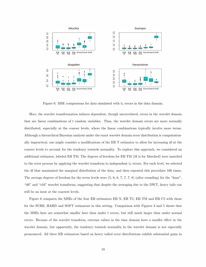
Figure 6: MSE comparisons for data simulated with t5 errors in the data domain.
Here, the wavelet transformation induces dependent, though uncorrelated, errors in the wavelet domain
that are linear combinations of t random variables. Thus, the wavelet domain errors are more normally
distributed, especially at the coarser levels, where the linear combinations typically involve more terms.
Although a hierarchical Bayesian analysis under the exact wavelet domain error distribution is computation-
ally impractical, one might consider a modifications of the EB T estimator to allow for increasing df at the
coarser levels to account for the tendency towards normality. To explore this approach, we considered an
additional estimator, labeled EB TM. The degrees of freedom for EB TM (M is for Matched) were matched
to the error process by applying the wavelet transform to independent t5 errors. For each level, we selected
the df that maximized the marginal distribution of the data, and then repeated this procedure 100 times.
The average degrees of freedom for the seven levels were (5, 6, 6, 7, 7, 7, 8) (after rounding) for the “haar”,
“d6” and “s16” wavelet transforms, suggesting that despite the averaging due to the DWT, heavy tails can
still be an issue at the coarsest levels.
Figure 6 compares the MSEs of the four EB estimators EB N, EB T5, EB TM and EB C5 with those
for the SURE, HARD and SOFT estimators in this setting. Comparison with Figures 3 and 5 shows that
the MSEs here are somewhat smaller here than under t errors, but still much larger than under normal
errors. Because of the wavelet transform, extreme values in the time domain have a smaller effect in the
wavelet domain, but apparently, the tendency towards normality in the wavelet domain is not especially
pronounced. All three EB estimators based on heavy tailed error distributions exhibit substantial gains in
18
efficiency over the standard methods, with EB TM performing only marginally better than EB T5 or EB
C5. With the exception of the SOFT estimator for the heavisine function, EB N offers improvement over
SURE, HARD and SOFT. As in the previous section, RSC performed poorly, obtaining larger MSEs than
all other methods for blocks, bumps, and doppler (average MSEs are 5.36, 47.46 8.73 respectively), with the
exception of heavisine, where it was comparable to EB N, but still not as good as EB T5, EB TM, or EB
C5.
5 GLINT Example
To observe their performance on a real data set, we applied our EB estimators to the GLINT data of Bruce
and Gao (1994). These data are radar reflections or glints measured in degrees for a rotating airplane
model, and are subject to errors that can be as large as 150 degrees in absolute value. The true signal is
supposed to be a low frequency oscillation about zero with possible level shifts, but the glint spikes are highly
non-Gaussian (Bruce and Gao 1994).
We used an estimate of σ = 29 so that 3 standard errors contain almost all of the glint spikes in the
original signal, based on information from Bruce and Gao (1994). In Figure 7, we compare the EB estimates
under the Normal-Normal and Bivariate t models to hard thresholding and the Robust-Smoother-Cleaner
wavelet transform of Bruce et al. (1994). In this example, shrinkage via hard thresholding has not removed
the glint spikes and Bruce and Gao (1994) view the resulting estimate of the signal as quite poor. The robust-
smoother-cleaner wavelet transform was designed to remove outlier patches from the wavelet decomposition,
and results in a much improved, smoother reconstruction than HARD thresholding (Bruce and Gao 1994).
While the EB normal estimate may still retain a spurious glint spike around t = 400, the EB shrinkage
estimates under the Bivariate t model with 3 degrees of freedom have effectively removed the outliers/non-
Gaussian glint spikes in the original signal. Unlike the RSC wavelet transform, the EB approach is completely
model based and can incorporate prior information about the process.
6 Discussion
In this article, we have proposed robust empirical Bayes methods for wavelet estimation. Embedding the
wavelet setup in a hierarchical normal scale mixture model, we obtain maximum likelihood estimates of the
unknown hyperparameters for each wavelet level, as well as an estimate of σ2 using data from all levels.
We then obtained shrinkage and threshold estimators based on posterior means under the estimated prior
distributions. When applied to a variety of simulated examples, these shrinkage estimators performed better
19
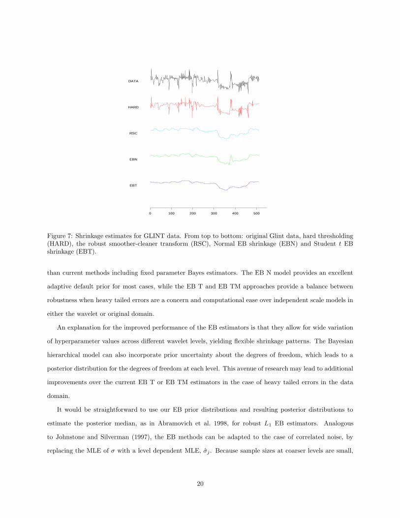
0 100 200 300 400 500
EBT
EBN
RSC
HARD
DATA
Figure 7: Shrinkage estimates for GLINT data. From top to bottom: original Glint data, hard thresholding(HARD), the robust smoother-cleaner transform (RSC), Normal EB shrinkage (EBN) and Student t EBshrinkage (EBT).
than current methods including fixed parameter Bayes estimators. The EB N model provides an excellent
adaptive default prior for most cases, while the EB T and EB TM approaches provide a balance between
robustness when heavy tailed errors are a concern and computational ease over independent scale models in
either the wavelet or original domain.
An explanation for the improved performance of the EB estimators is that they allow for wide variation
of hyperparameter values across different wavelet levels, yielding flexible shrinkage patterns. The Bayesian
hierarchical model can also incorporate prior uncertainty about the degrees of freedom, which leads to a
posterior distribution for the degrees of freedom at each level. This avenue of research may lead to additional
improvements over the current EB T or EB TM estimators in the case of heavy tailed errors in the data
domain.
It would be straightforward to use our EB prior distributions and resulting posterior distributions to
estimate the posterior median, as in Abramovich et al. 1998, for robust L1 EB estimators. Analogous
to Johnstone and Silverman (1997), the EB methods can be adapted to the case of correlated noise, by
replacing the MLE of σ with a level dependent MLE, σj . Because sample sizes at coarser levels are small,
20
there may be substantial uncertainty in the EB estimators of cj , wj and σj . In cases with small signal-to-
noise ratios, improved estimation can be achieved using Gibbs sampling (Clyde et al. 1998) combined with
Rao-Blackwellized estimators. If the computational issues for this approach could be simplified, this would
be a promising competitor to our methods, and would provide improved estimates over a naive EB approach
that ignores uncertainty in the hyperparameter estimates.
References
Abramovich, F., Sapatinas, T., and Silverman, B.W. (1998). Wavelet thresholding via a Bayesian approach.
Journal of the Royal Statistics Society, Series B, 60, 725–749.
Andrews, D. F. and Mallows, C. L. (1974). Scale mixtures of normal distributions. Journal of the Royal
Statistical Society, Series B, 36, 99–102.
Bruce, A., Donoho, D, Gao, H-Y, and Martin, D. (1994). Denoising and robust nonlinear wavelet analysis.
In SPIE Proceedings, Wavelet Applications, Volume 2242, Orlando, FL.
Bruce, A. and Gao, H-Y. (1994). S+Wavelets, Users Manual. Seattle: StatSci.
Chipman, H., Kolaczyk, E., and McCulloch, R. (1997). Adaptive Bayesian wavelet shrinkage. Journal of
the American Statistical Association, 92, 1413–1421.
Clyde, M., Parmigiani, G., Vidakovic, B. (1998). Multiple shrinkage and subset selection in wavelets.
Biometrika, 85, 391–402.
Dempster, A.P. Laird, N.M. and Rubin, D.B. (1977). Maximum likelihood estimation from incomplete data
via the EM algorithm (with discussion). Journal of the Royal Statistical Society, Series B, 39, 1–38.
Donoho, D.L., and Johnstone, I.M., (1994). Ideal spatial adaptation by wavelet shrinkage. Biometrika, 81,
425–256.
Donoho, D. and Johnstone, I. (1995). Adapting to unknown smoothness via wavelet shrinkage. Journal of
the American Statistical Association, 90, 1200–1224.
Donoho, D., Johnstone, I., Kerkyacharian, G., and Picard, D. (1995). Wavelet shrinkage: Asymptopia?
Journal of the Royal Statistical Society, series B, 57, 301–369.
21
Fan, T-H, and Berger, J.O. (1990). Exact convolutions of t distributions with applications to Bayesian
inference for a normal mean with t prior distributions. Journal of Statist. Comput. Simul., 36,
209–228.
George, E.I. (1986). Minimax multiple shrinkage estimation. Annals of Statistics, 14, 188–205.
George, E.I. and Foster, D.P. (1997). Calibration and empirical Bayes variable selection. Tech Report,
University of Texas, at Austin.
Johnstone, I.M. and Silverman, B.W. (1997). Wavelet threshold estimators for data with correlated noise.
Journal of the Royal Statistical Society, Series B, 59, 319–351.
Johnstone, I.M. and Silverman, B.W. (1998). Empirical Bayes approaches to mixture problems and wavelet
regression. Tech Report. University of Bristol.
O’Hagan, A. (1979). On outlier rejection phenomena in Bayes inference. Journal of the Royal Statistical
Society, Series B, 41, 358–367.
O’Hagan, A. (1988). Modelling with heavy tails. Bayesian Statistics 3, eds. J.M. Bernardo, M.H. DeGroot,
D.V. Lindley, and A.F.M. Smith, Oxford, U.K. Clarendon Press, pp. 345–359.
Thisted, R. A. (1988). Elements of Statistical Computing. Chapman Hall.
West, M. (1984). Outlier models and prior distributions in Bayesian linear regression. Journal of the Royal
Statistical Society, Series B, 46, 431–439.
West, M. (1987). On scale mixtures of normal distributions. Biometrika, 74, 646–648.
22