Embed Size (px)
Citation preview

Principal Components Analysis
Transformation of data into new variables

Motivation
• Scatterplots– Good for two variables at a time– Disdvantage:may miss complicated relationships
• Projections along different directions may detect them– Say along direction defined by 2x1+3x2+x3=0

Projection pursuit methods
• Allow searching for “interesting” directions• Interesting means maximum variability• Data in 2-d space projected to 1-d:
Data
Shows
Little
Variation Data Shows
Greater Variability
x2
x1
2x1+3x2=0
0
0 3] 2[2
1
=
=⎥⎦
⎤⎢⎣
⎡
xa
xx
t
Projection Task is to find a

Principal Components
• Find linear combinations that maximize variance subject to being uncorrelated with those already selected
• Hopefully there are few such linear combinations-- known as principal components
• Task is to find a k-dimensional projection where 0 < k < d-1

Principal Components AnalysisX = n x p data matrix of n cases
p variablesx(1)
x(i) is a p x 1column vector
Each row of matrixis of the form x(i)T
x(i)
x(n)
Assume X is mean-centered, so that the value of each variable issubtracted for that variable
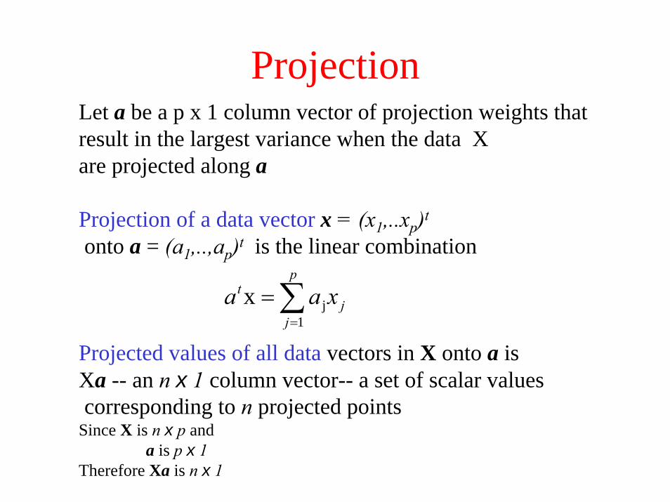
ProjectionLet a be a p x 1 column vector of projection weights thatresult in the largest variance when the data X are projected along a
Projection of a data vector x = (x1,..xp)t
onto a = (a1,..,ap)t is the linear combination
∑=
=p
jj
t xaa1
jx
Projected values of all data vectors in X onto a isXa -- an n x 1 column vector-- a set of scalar valuescorresponding to n projected points
Since X is n x p and a is p x 1
Therefore Xa is n x 1
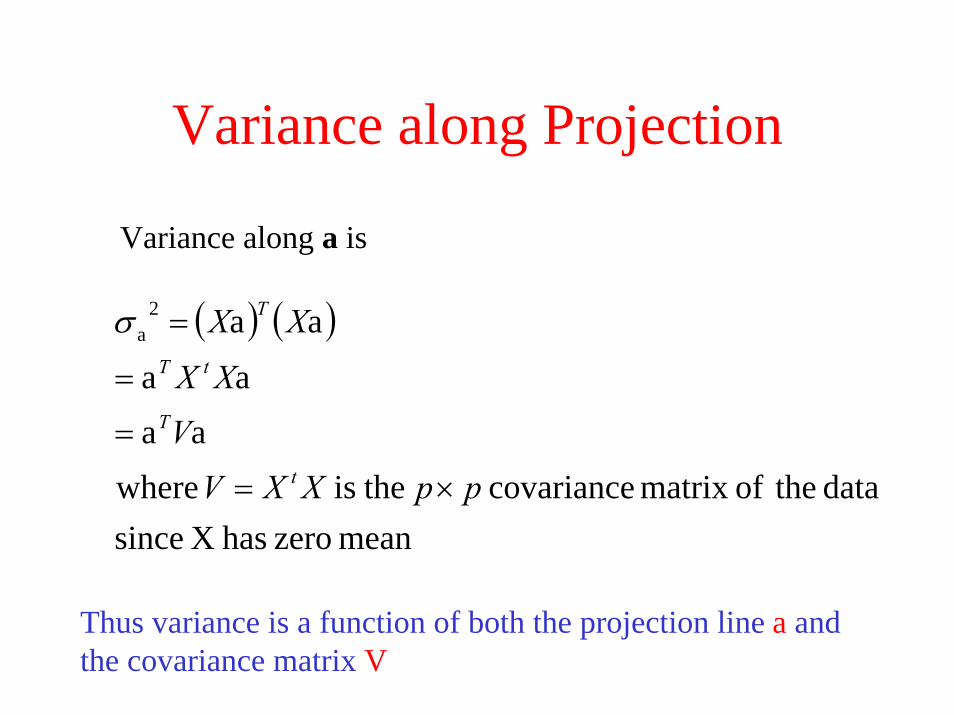
Variance along Projection
Variance along a is
( ) ( )
meanzero has X sincedata theofmatrix covariance theis where
aaaa
aa2a
ppXXVV
XX
XX
t
T
tT
T
×=
=
=
=σ
Thus variance is a function of both the projection line a and the covariance matrix V

Maximization of VarianceMaximizing variance along a is not well-defined since
we can increase it without limit by increasing the size of the components of a.
Impose a normalization constraint on the a vectors such thataTa = 1
Optimization problem is to maximize )1( −−= aaVaau tt λ
Where lambda is a Lagrange multiplier.Differentiating wrt a yields
0I)-(V toreduceswhich
022
=
=−=∂∂
a
aVaau
λ
λ
Characteristic Equation!

What is the Characteristic Equation?
Given a d x d matrix M, a very important class of linearEquations is of the form λxMx =
dxd dx1 dx1
which can be rewritten as 0)( =− xIM λ
If M is real and symmetric there are d possible solution Vectors, called Eigen Vectors, e1, edand associated Eigen values
dλλ ,...,1

Principal Component is obtained from the Covariance Matrix
If the matrix V is the Covariance matrixThen its Characteristic Equation is
0)( =− aIV λRoots are Eigen ValuesCorresponding Eigen Vectors are principal components
First principal component is the Eigen Vector associatedwith the largest Eigen value of V.

Other Principal Components
• Second Principal component is in direction orthogonal to first
• Has second largest Eigen value, etc
First PrincipalComponent e1
X2
SecondPrincipalComponente2
X1
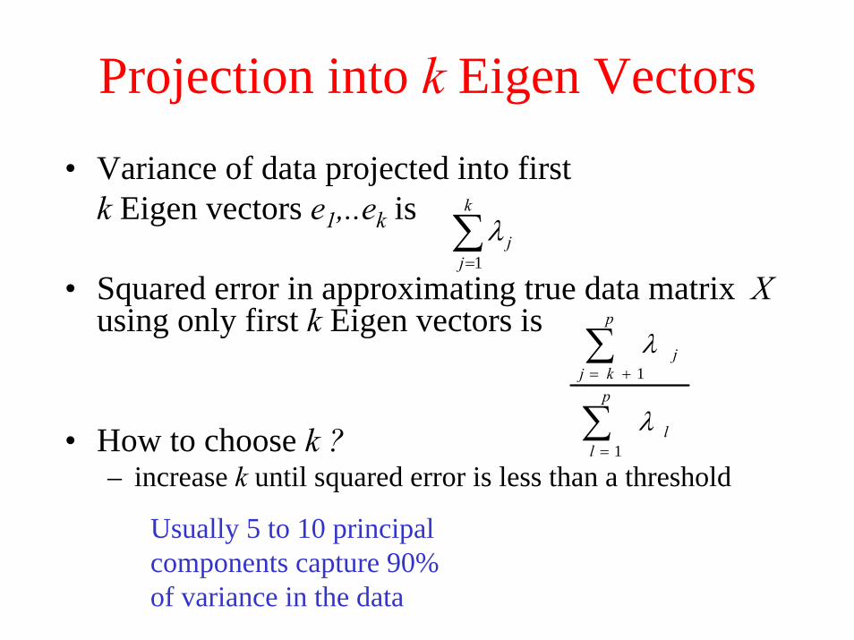
Projection into k Eigen Vectors
• Variance of data projected into firstk Eigen vectors e1,..ek is
• Squared error in approximating true data matrix X using only first k Eigen vectors is
• How to choose k ?– increase k until squared error is less than a threshold
∑=
k
jj
1
λ
∑
∑
=
+=p
ll
p
kjj
1
1
λ
λ
Usually 5 to 10 principalcomponents capture 90%of variance in the data

Scree PlotAmount of varianceexplained by eachconsecutiveEigen value
CPU data8 Eigen values:63.2610.7010.306.685.232.181.310.34
Weights put byfirst component e1
on eight variables are:0.199-0.365-0.399-0.336-0.331-0.298-0.421-0.423
Eigen values of Correlation Matrix
An example Eigen Vector
Scatterplot Matrix
CPU data
Eigen Value numberP
erce
ntV
aria
nce
Exp
lain
edExample of PCA

PCA using correlation matrix and covariance matrix
Proportions ofvariation attributableto different components:96.023.930.040.010000
Scree PlotCorrelationMatrix
Scree PlotCovarianceMatrix
Eigen Value number
Eigen Value number
Per
cent
Varia
nce
Expl
aine
dP
erce
ntVa
rianc
e Ex
plai
ned

Graphical Use of PCA
First twoprincipal componentsof six dimensional data17 pills (data points)Six values are times at whichspecified proportionof pill has dissolved:10%, 30%, 50%, 70%, 75%, 90%
Principal Component 1
Prin
cipa
l Com
pone
nt 2
Pill 3 is very different
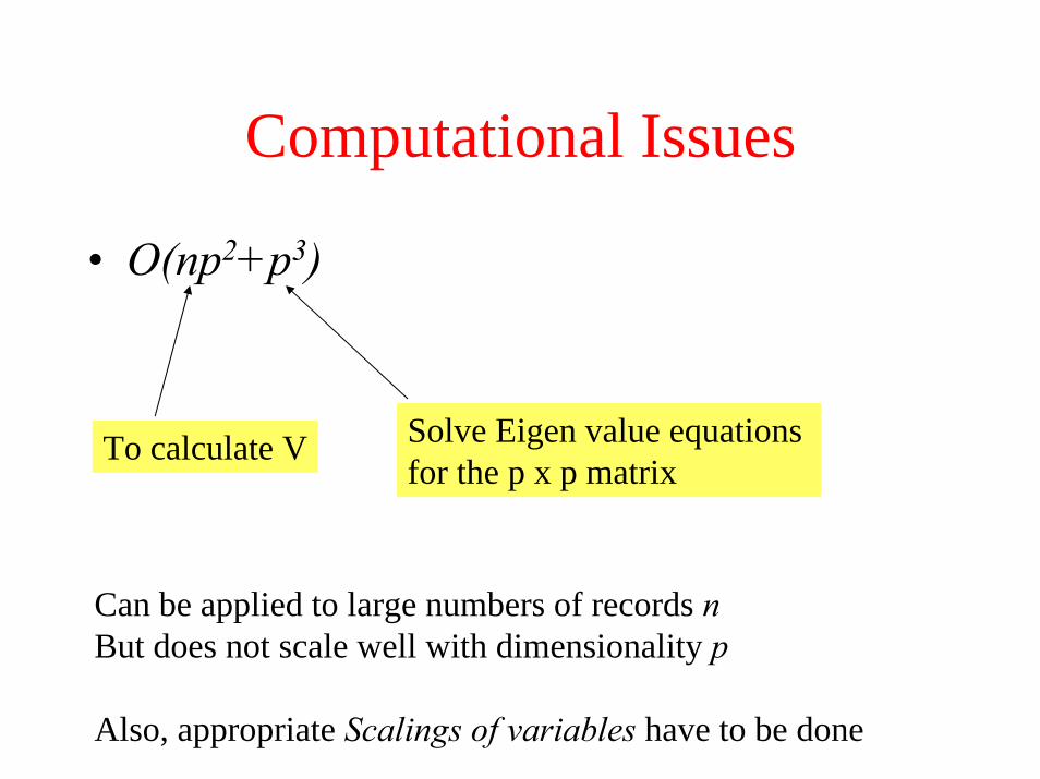
Computational Issues
• O(np2+p3)
To calculate V Solve Eigen value equations for the p x p matrix
Can be applied to large numbers of records nBut does not scale well with dimensionality p
Also, appropriate Scalings of variables have to be done

Multidimensional Scaling
• Detecting underlying structure– e.g., data lies on a string or surface in multi-
dimensional space• Distances are preserved
– Distances between data points are mapped to a reduced space
• Typically displayed on a two-dimensional plot

Multidimensional Scaling Plot of Dialect SimilaritiesNumerical codes of villages and their counties
Each Pair of villages rated by percentage of 60 items for which villagersUsed different words We are able to visualize 625 distances intuitively
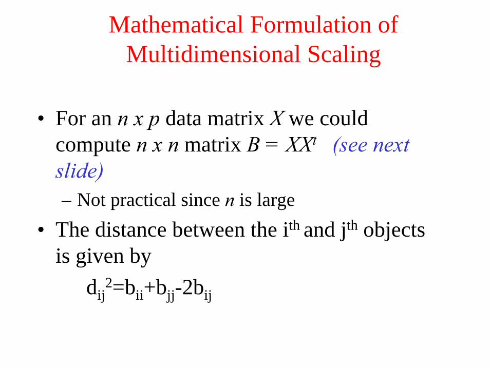
Mathematical Formulation of Multidimensional Scaling
• For an n x p data matrix X we could compute n x n matrix B = XXt (see next slide)– Not practical since n is large
• The distance between the ith and jth objects is given by
dij2=bii+bjj-2bij

XtX versus XXt
• If X is n x p p=4
• XtX is p x p
• XXt is n x n
⎥⎥⎥⎥
⎦
⎤
⎢⎢⎢⎢
⎣
⎡
4321
24232221
14131211
....
nnnn xxxx
xxxxxxxx
⎥⎥⎥⎥⎥⎥
⎦
⎤
⎢⎢⎢⎢⎢⎢
⎣
⎡
=
⎥⎥⎥⎥
⎦
⎤
⎢⎢⎢⎢
⎣
⎡
×
⎥⎥⎥⎥
⎦
⎤
⎢⎢⎢⎢
⎣
⎡ ∑∑==
n
iii
n
ii
nnnnn
n
n
n xxx
xxxx
xxxxxxxx
xxxxxxxxxxxx
121
1
21
4321
24232221
14131211
42414
32313
22212
12111
,.......
⎥⎥⎥⎥⎥⎥
⎦
⎤
⎢⎢⎢⎢⎢⎢
⎣
⎡=
=
⎥⎥⎥⎥
⎦
⎤
⎢⎢⎢⎢
⎣
⎡
×
⎥⎥⎥⎥
⎦
⎤
⎢⎢⎢⎢
⎣
⎡ ∑∑==
n
n
n
ni
jjj
j
n
n
n
n
nnnn bbbbbbbbb
bxxbxb
xxxxxxxxxxxx
xxxx
xxxxxxxx
44241
33231
22221
1
4
12112
4
1
2111
42414
32313
22212
12111
4321
24232221
14131211
.
.
.
.
.
.
.
.
,...
n x pp x n px p
nxp pxn nxn
CovarianceMatrix
B Matrix containsdistanceinformationdij
2=bii+bjj-2bij
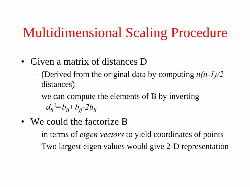
Multidimensional Scaling Procedure
• Given a matrix of distances D – (Derived from the original data by computing n(n-1)/2
distances) – we can compute the elements of B by inverting
• We could the factorize B– in terms of eigen vectors to yield coordinates of points – Two largest eigen values would give 2-D representation
dij2=bii+bjj-2bij

Inverting distances to get Bdij
2=bii+bjj-2bij
• Summing over i
• Summing over j
• Summing over i and j
jji
ij nbBtrd +=∑ )(2
iii
ij nbBtrd +=∑ )(2
)(22 Bntrdi
ij =∑Can obtain tr(B)
Can obtain bii
Can obtain bjj
Thus expressing bij as a function of dij2
Method is known as Principal Coordinates Method

Classical Multidimensional Scaling into Two Dimensions
• Minimize
2)( iji j
ij d−∑∑ δ
Observed distance betweenpoints i and j in p-space
Distance between thepoints in two-dimensionalspace
Criterion is invariant wrt rotations and translations.However it is not invariant to scalingBetter criterion is or
∑
∑∑ −
jiij
iji j
ij
d
d
,
2
2)(δ
∑
∑∑ −
jiij
iji j
ij
d
d
,
2
2)(δ Calledstress
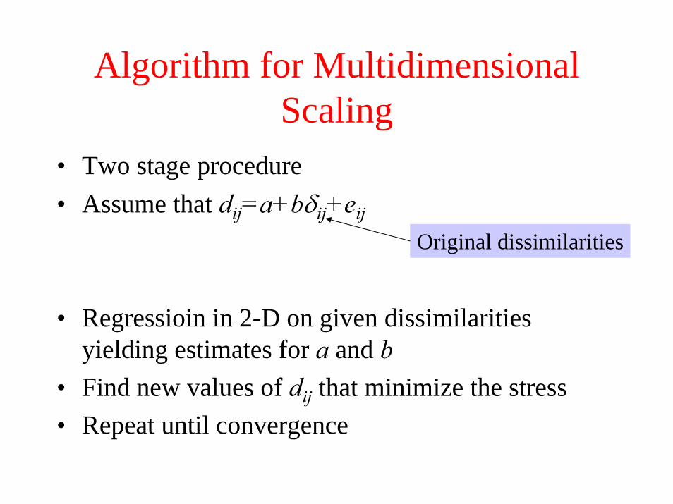
Algorithm for Multidimensional Scaling
• Two stage procedure• Assume that dij=a+bδij+eij
• Regressioin in 2-D on given dissimilarities yielding estimates for a and b
• Find new values of dij that minimize the stress• Repeat until convergence
Original dissimilarities
Variations of Multidimensional Scaling
• Above methods are called metric methods• Sometimes precise similarities may not be
known– only rank orderings• Also may not be able to assume a particular
form of relationship between dij and δij– Requires a two-stage approach– Replace simple linear regression with
monotonic regression

Disadvantages of Multidimensional Scaling
• When there are too many data points structure becomes obscured
• Highly sophisticated transformations of the data (compared to scatter lots and PCA)– Possibility of introducing artifacts– Dissimilarities can be more accurately determined
when they are similar than when they are very dissimilar
• Horseshoe effect when objects manufactured in a short time span differ greatly from objects separated by greater time gap
• Biplots show both data points and variables