Embed Size (px)
Citation preview

Transient outage model considering corrective and preventivemaintenance
Guoqiang JI1, Wenchuan WU1, Boming ZHANG1, Hongbin SUN1
Abstract Traditional outage model for the power equip-
ment usually focus on the behavior of the equipment under
random factors, and the availability of the power equip-
ment in system analysis is usually confined to the steady
value. However, this model may be inaccurate in the short
term analysis, where the transient process of availability
has not ended yet. Furthermore, the power equipment in the
short term analysis might be influenced by both random
factors and deterministic factors, yet the impact of deter-
ministic factors cannot be completely reflected in the tra-
ditional outage model. Based on the above issues, a
Markov-based transient outage model is proposed in this
paper, which describes the deterioration and repair process
of an equipment. Both the corrective maintenance and
preventive maintenance are concerned in the model. The
preventive maintenance in the model is considered as
deterministic event, in which the start time and duration are
both scheduled. Meanwhile the corrective maintenance and
the unexpected failure are modeled as random events. The
transient state probability and availability of equipment
under preventive maintenance is derived. The effect of
deterministic events on the availability of equipment is
analyzed on numerical tests. The proposed model can be
used in the short-term reliability assessment and mainte-
nance scheduling in actual systems.
Keywords Outage model, Preventive maintenance,
Corrective maintenance, Markov process, Transient
availability
1 Introduction
The power system usually faces many uncertain factors,
such as the variation of the load, the changes of the
weather, and the unexpected outage of the power equip-
ment, which bring great risk to the system operation and
control. Risk assessment has become an important tool to
support the decision making of the power system nowa-
days, and the accuracy of the risk assessment depends
greatly on the outage model of the power equipment.
The outage model describes the stochastic behavior of
the power equipment under various factors, and there have
been many research achievements in this area.
The Markov process based model is the most commonly
used mathematical model which can be solved analytically
[1, 2]. Various states, such as normal, abnormal, outage and
so on which provide a complete description of the
stochastic process of equipment can be contained in the
state diagram of Markov model [3]. The Markov model is
very suitable for the case that all factors which influence
the equipment are random. The two-state Markov model is
the simplest outage model to describe the alternation
CrossCheck date: 22 September 2015
Received: 19 June 2014 / Accepted: 29 September 2015 / Published
online: 22 July 2016
� The Author(s) 2016. This article is published with open access at
Springerlink.com
& Wenchuan WU
Guoqiang JI
Boming ZHANG
Hongbin SUN
1 Tsinghua University, Beijing, China
123
J. Mod. Power Syst. Clean Energy (2016) 4(4):680–689
DOI 10.1007/s40565-016-0201-z
process of operating and failure, which has been used
widely in traditional reliability analysis [4]. In order to
demonstrate the equipment behavior more accurately, the
operating and repair state has been classified further into
several sub-states. In [5–8], the outage model is repre-
sented by the state transition diagram which contains
deterioration, inspection, maintenance and other states. The
equipment is inspected and maintained periodically and the
optimal inspection or maintenance frequency is calculated
to obtain the minimal cost or the maximal availability.
Similar results can also be found in many other areas
[9–11]. In [12, 13], the authors point out that the classical
maintenance model may be inaccurate compared to the real
world especially when the inspection rates are non-peri-
odic, and a new Markov state diagram is proposed to solve
the problem, the basic idea of which is to divide the
original deterioration process into several sub deterioration
processes. Beside the Markov models, there are also other
outage models which demonstrate the deterioration and
repair process of equipment in different ways, for instance,
the Kijima I and II models [14–17], with much more
amount of calculation.
Most of the existing literatures relating to the outage
model only focus on the steady state of the equipment;
namely, the state probability of the equipment is constant
and does not change with time. This kind of models is
applicable to the long time scale (usually several years or
longer) problems, such as the reliability analysis, capacity
expansion, network planning and so on, in which the steady
value of the state probability of power equipment is
accurate enough. But in the short term problems (usually
several weeks or months), the use of steady outage model
may bring significant error, which will be explained in the
next section. However, there are few literatures concerning
about the special features of the outage model used in the
short term problems.
Generally speaking, there are two kinds of features in
the outage model used in the short term problems.
1) Transient availability
The outage model used in short-term problems should
be transient model, which means the probability of states in
the model should be time-varying. In the long term prob-
lems, the transient process of the state probability of
equipment is usually neglected since the period of the
transient process is extremely short compared to the whole
time scale. However, in the short term problems, the period
of the transient process is in the same order of magnitude of
the whole time scale to be considered.
2) Coexistence of random factors with deterministic
factors
In the short term problems, the deterministic factors and
the random factors usually coexist together, both of which
affect the behavior of the power equipment together. In the
long term problems, almost all the factors, no matter
environmental or human, can be regarded as random fac-
tors because of the characteristics of long time scale.
However, in the short term problems, the factors related to
the human subjective intention should be more treated as
deterministic factors, such as the maintenance schedule for
certain power equipment in the next few weeks. The
starting and ending time of these deterministic events
should not be changed arbitrarily and randomly according
to the common sense and operation characteristics of
power system. However, in the traditional steady model,
the effect of deterministic factors on the behavior of the
equipment can hardly be considered since the impact
cannot be reflected on the steady value of the state prob-
ability of the equipment.
Based on the above analysis, a new outage model which
is applicable to the short term problems is proposed in this
paper. The transient probability is considered in this model
and both the random and deterministic factors are incor-
porated. The paper is organized as follows. In Section 2,
the comparison of the transient model and steady model is
given to show the necessity of the transient probability.
The basic Markov model is presented in Section 3, which
only considers the random factors same as conventional
models for long term problems. The deterministic factors in
the short term problems are added to the outage model in
Section 4. The comparisons of proposed model and the
conventional model are shown through some examples in
Section 5. In Section 6 there are some conclusions.
2 Comparison between transient model and steadymodel
Firstly, a simple example will be given to show the
difference between the transient model and steady model,
which explains the necessity of the research on transient
model.
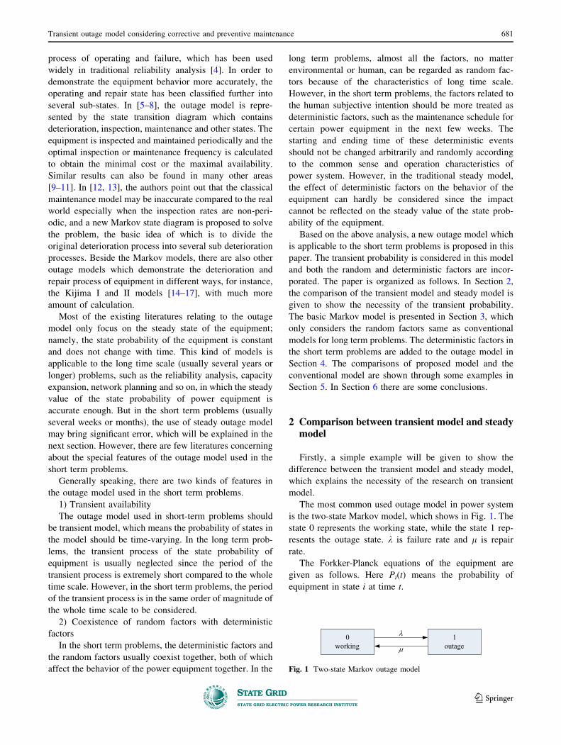
The most common used outage model in power system
is the two-state Markov model, which shows in Fig. 1. The
state 0 represents the working state, while the state 1 rep-
resents the outage state. k is failure rate and l is repair
rate.
The Forkker-Planck equations of the equipment are
given as follows. Here Pi(t) means the probability of
equipment in state i at time t.
0working
1outage
Fig. 1 Two-state Markov outage model
Transient outage model considering corrective and preventive maintenance 681
123

dP0 tð Þdt
¼ �kP0 tð Þ þ lP1 tð Þ
dP1 tð Þdt
¼ kP0 tð Þ � lP1 tð Þ
8>><
>>:
ð1Þ
It should be noticed that (1) are differential equations,
and it is a common sense that the summation of all the state
probability equals to 1 at any time. Once the initial state of
the equipment is known, (1) can be solved and the
expression of Pi(t) can be obtained. Suppose the equipment
is working at time t = 0, then the expressions of Pi(t) can
be shown as follows.
P0 tð Þ ¼ lkþ l
þ kkþ l
e� kþlð Þt
P1 tð Þ ¼ kkþ l
� kkþ l
e� kþlð Þt
8>><
>>:
ð2Þ
It is defined that availability A(t) is the probability that
the equipment is in working state at time t, and
unavailability U(t) is the probability that in outage state
at time t. Obviously, in the two-state Markov model,
A(t) = P0(t), U(t) = P1(t).
The outage model with (1) can be called the transient
model, the feature of which is that the availability and
unavailability of the equipment vary with time and the
expressions of the state probability contain exponential
terms. However, usually in the traditional analysis, only
the steady model is considered. The steady model is
actually the transient case with the time t ? ?. In this
case, the differential (1) turn to algebraic equations as
follows.
0 0½ � ¼ P0 tð Þ P1 tð Þ½ � �k kl �l
� �
ð3Þ
Obviously, the calculation of (3) is much more easier
than that of (1), and the availability and unavailability
obtained from (3) are A(t) = l/(k ? l), U(t) = k/(k ? l),both of which are commonly used in the traditional
reliability analysis. It should be noted that the steady model
can only be used under the premise that the time tends to
infinity.
The curves of unavailability of transient model and
steady model are shown in Fig. 2. Usteady is the steady
value of unavailability and
From Fig. 2 it is clear that at the beginning of the time
period, the difference between transient unavailability and
steady unavailability is distinct. The period that the tran-
sient value varies with time significantly can be called the
transient period. Suppose the criterion for the end of the
transient period is |1 - U(t)/Usteady| B e, where e is the
threshold value, then the duration of the transient period
can be calculated as follows.
Ttransient �1
kþ lln1
eð4Þ
The duration of the transient period depends on the
transition rate k and l. According to the common sense in
the power system, the maintenance time for the important
equipment, such as transformer, may last for several days
or even several weeks. Suppose the threshold value
e = 10%, the duration of the transient period of the state
probability for the power equipment may be plenty of
weeks.
Therefore, whether to choose the transient model in the
system analysis depends on the relative magnitude between
the duration of transient period and the whole time scale to
be studied. In the long term planning of the power system
where the time scale usually covers for years, the transient
period can be ignored and the steady model of the power
equipment can be used. However, in some short term
research, such as the maintenance scheduling or the risk
assessment in the near future, the time period to be con-
sidered is just next month or next quarter. In this case, the
used of steady model may bring appreciable error since the
state probability of the power equipment is still in the
transient period in most of the time. Hence, in this case, the
transient model should be considered to describe the
behavior of the power equipment in the short term more
accurately.
3 Markov-based equipment outage modelconsidering corrective maintenance
The influncing factors of power equipment can be
classified into two categories, random and deterministic
factors. In this section, a Markov process model which
describe the stochastic behavior of power equipment is
0 10 20 30 40 50 60 70 80 90 100
0.010.020.030.040.050.060.070.080.090.10
t (day)
Una
vaila
bilit
y
Steady
U t
steadyUTransient
Fig. 2 Curves of unavailability of the equipment
682 Guoqiang JI et al.
123

constructed. Transient availability is considered here to
correlate with the first feature proposed in Section 1. In the
next section, deterministic factors will be added to the
model to reflect the second feature.
Deterioration and failure are two major random factors for
power equipment. Themaintenancewhich is carried outwhen
a failure occurs is defined as Corrective Maintenance (CM)
[18], the aim of which is to restore the equipment to operable
condition. Obviously, CM should be treated as random event
and the start time or the duration of CM is unpredictable.
Deterioration of power equipment is an agonizingly
slow and irreversible process. From the physical sense, the
deterioration process of equipment is a non-Markov pro-
cess, which means the transition rates between states are
time-varying. However, the non-Markov model can hardly
be solved analytically. In the traditional research, the
deterioration process is usually modeled by multi-state
Markov process on analytic calculation grounds.
The alternate process of operation and failure can be
expressed by state transition diagram. A multi-state Mar-
kov model is shown in Fig. 3, which is the most commonly
used model in previous literatures [13].
In Fig. 3, Numbers 1 * N are the stages of deteriora-
tion and number N ? 1 is failure state caused by deterio-
ration. kij means the transition rate from state i to state j,
and l means the repair rate of CM after failure caused by
deterioration.
The differential equations of the model in Fig. 3 are
shown as (5).
dP
dt¼ P
�k12 k12. .. . .
.
�kN�1;N kN�1;N
�kN kNl �l
2
666664
3
777775
P ¼ P1 tð Þ P2 tð Þ � � � PN tð Þ PNþ1 tð Þ½ �
8>>>>>>><
>>>>>>>:
ð5Þ
In (5), P1 * PN means the probability of deterioration
state 1 * N and PN?1 means the probability of failure state
N ? 1. Suppose the initial state of equipment at time t = 0 is
S0 (S0 = 1, 2,…, N), the equations above can be solved
according to Laplace transformation. The mathematical
expression of transient probability for each state is the
summation of steady value of the probability and several
exponential terms damping with time, which is shown as (6).
PS0k tð Þ ¼ Pk1 þ
XN
i¼1
Lki e�si t k ¼ 1; 2; . . .;N þ 1 ð6Þ
where the superscript S0 is the initial state of the equip-
ment; Pk1 is the steady value of probability for state k; Lkiis the coefficient for ith exponential term and si is the
corresponding damping exponent, both of which can be
calculated by solving the (5). The detail of the calculation
is given in Appendix A.
Based on the expression of transient probability for each
state, the expression of transient availability can be esti-
mated as below. In Fig. 3, states from number 1 to number
N are all working states, although with different deterio-
ration. Hence, the availability of equipment in Fig. 3 is the
summation of the probability from P1 to PN.
AS0 tð Þ ¼XN
k¼1
PS0k tð Þ ð7Þ
The superscript S0 means the initial state of the
equipment as well. Obviously, the transient availability is
also a time-varying function and it will graduate to the
steady availability when time tends to infinity.
4 Markov-based equipment outage modelconsidering corrective and preventivemaintenance
Besides CM, there is another kind of maintenance for
power equipment called Preventive Maintenance (PM). PM
is the maintenance which is carried out regularly on power
equipment in operation. The aim of PM is to improve the
working condition of the equipment although there is no
failure occuring temporarily.
In the power systems, periodic inspection will be carried
on the power equipment and if necessary, PM may be exe-
cuted to improve the working condition of the equipment. If
the inspection result shows that the status of equipment is
poor, PM may be scheduled in a short time(several days or
weeks, e.g.), otherwise PM might be scheduled after a long
time (severalmonths, e.g.) or even no need tomaintain. After
PM, the equipment will return to working state.
Figure 4 shows a simple example of state transition
diagram considering the inspection and maintenance in
long term[12-13]. Here the meanings of 1 * N?1, kij, andl are the same as before. The meanings of other symbols
1 212 k k+1, 1k k N+1N N
Fig. 3 Multi-state Markov equipment outage model
1 k k+1 N+1
I1 Ik+1Mk+1Ik
12 1,k k , 1k k 1, 2k k N
11 k
k
1k
1k
1k
Fig. 4 Simple example of Markov outage model considering
inspection and PM
Transient outage model considering corrective and preventive maintenance 683
123

are the same as literature [12, 13]. Ik and Mk means the
inspection state and maintenance state respectively. rkmeans
the inspection rate and xk means the repair rate of planned
maintenance. nk is the transition rate between Ik andMk.
In Fig. 4, the maintenance, including PM and CM, are
all treated as random events and modeled as states in the
Markov process. However, as mentioned before, some
factors which affect the behavior of equipment in short
term problems shows strong characteristic of determinacy.
If the period to be considered here is from the end of
inspection to the end of PM, which may be a few days or
several weeks, the risk assessment and maintenance
scheduling in this period forms a short term problem which
can be regarded as a part of the long term model in Fig. 4.
In this case, PM, the start time and end time of which are
predetermined according to the inspection result and other
objective conditions, is the typical example of the deter-
ministic events.
The time axis of the inspection and PM in the short term
problem is shown in Fig. 5. M means the start time of PM
and d means the duration of PM, both of which are
deterministic.
Based on the above analysis, it is necessary to propose a
new model which is applicable to the short term problem.
Before introducing the new model, the following precon-
ditions are given.
1) Noticed that the equipment with PM is usually the
one with bad working condition and the failure rate of the
equipment may be higher than the one with normal con-
dition. Hence during this short term period, the equipment
may suffer from unexpected failures, so the outage model
contains deterioration and failure state as usual.
2) The time after inspection is set to be the initial time
(t = 0) of the short term period, and the working condition
of the equipment at this time is known. The deterministic
PM is scheduled in the near future according to the
inspection result and other factors.
3) The state of the equipment at time 0, M and
M ? d can be expressed as S0, SM and SM?d, respectively,
and only the state S0 is known. The state SM depends on the
stochastic deterioration process and the difference between
SM and SM?d depends on the effect of PM.
4) Similar to the previous literatures, it is supposed that
after PM the equipment will return to the previous state by
one stage, like the model in Fig. 4. If the equipment is in
D1, after PM it will return to D1 again. It’s obvious that this
assumption can be easily relaxed or generalized and the
analytic procedure will be similar [7].
5) Once an unexpected failure occurs, the CM will be
executed on the equipment and the state of the equipment
will return to D1 after CM as shown in Fig. 3. It is apparent
that this assumption can also be easily relaxed and the
analytic procedure is similar.
Based on the above preconditions, the calculation
method of transient availability of the outage model used in
the short term problem is given below.
There are two possible cases to be considered in the
short term problem.
4.1 Case A: no unexpected failure occurs
before time M
The probability of this case can be calculated as follows.
PcaseA ¼ 1� HS0 Mð Þ ð8Þ
where HS0 tð Þ is the probability cumulative distribution
function of equipment life and the superscript S0 represents
the initial state of the equipment. The detailed expression
of HS0 tð Þ is given in Appendix B.
In this case, the equipment keeps working during the
period [0, M] and the PM will be implemented as usual
during the period [M,M ? d]. The equipment will return to
operation after PM with better working condition.
Due to the irreversibility of natural deterioration, the
state of the equipment at time t (0\ t\M) .i.e. St can be
any state between S0 to N. Given the premise that the
equipment keeps running during the period [0, M], the
probability of the equipment in state k at time t is a con-
ditional probability, which can be denoted as
PS0conk tð Þ; k ¼ 1; 2; � � � ;N. The expression of PS0
conk tð Þ is
given in Appendix C. As mentioned before, the state SM?d
depends entirely on the state SM. So once the probability
PS0conk Mð Þ is obtained, the probability of the equipment in
each state after PM, denoted as PS0SMþd
, is already known as
well, which is also shown in Appendix C.
Hence the equipment’s availability in case A is given as
below. Noticed that the availability from time 0 to time M
equals to 1 in this case since it is supposed that the
equipment keeps working from time 0 to time M.
AS0caseA t;Mð Þ ¼
1; t 2 0;M½ Þ0; t 2 M;M þ d½ ÞPN
SMþd¼1
ASMþd t �M � dð ÞPS0SMþd
t 2 M þ d;þ1½ Þ
8>>>><
>>>>:
ð9ÞM M d t0
Preventive maintenanceinspection
Time period for short term problem
Fig. 5 Time axis of the inspection and PM
684 Guoqiang JI et al.
123
4.2 Case B: unexpected failure occurs
before time M
The probability of this case can be calculated as below.
PcaseB ¼ HS0 Mð Þ ð10Þ
In this case, the scheduled PM will not be implemented
as usual since an unexpected contingency occurs. The CM
should be carried out immediately after the failure and the
original PM will be canceled. After CM, the state of the
equipment will return to D1.
The availability in this case is
AS0caseB t;Mð Þ ¼ 1� HS0
tru t;Mð Þ þ A1 tð Þ � wS0tru tð Þ ð11Þ
where � means convolution; A1 tð Þ is the transient
availability function with initial state S0 = 1; HS0tru t;Mð Þ
is the truncated probability cumulative distribution
function of equipment life under the assumption that a
failure will occur before time M and wS0tru tð Þ means the
probability density function of the first renewal period of
the equipment. Their expressions of both are given in
Appendix B.
Make a synthesis of the two cases, the equipment’s
availability in the new model can be obtained as (12). The
subscript ‘‘tru’’ represents that the availability is ‘‘trun-
cated’’ by the deterministic PM.
AS0tru t;Mð Þ ¼ PcaseAA
S0caseA t;Mð Þ þ PcaseBA
S0caseB t;Mð Þ ð12Þ
Since the main focus of this paper is on deterioration
and the maintenance for eliminating the damage caused by
deterioration, the failures caused by random environmen-
tal factors are not considered in Fig. 3. When considering
the environmental factors, the analytic procedure of the
new outage model will be similar, which is given in
Appendix D.
5 Numerical examples
Some practical examples are analyzed in this section to
show the effect of deterministic PM on the outage
model.
Take the transformer as an example. The outage model
for transformer in short term period is the most represen-
tative model which contains both random and deterministic
factors. According to the IEEE standards [19], the states of
transformer are usually classified into four categories,
which are normal, attentive, abnormal and fault. The nor-
mal, attentive and abnormal states are usually treated as
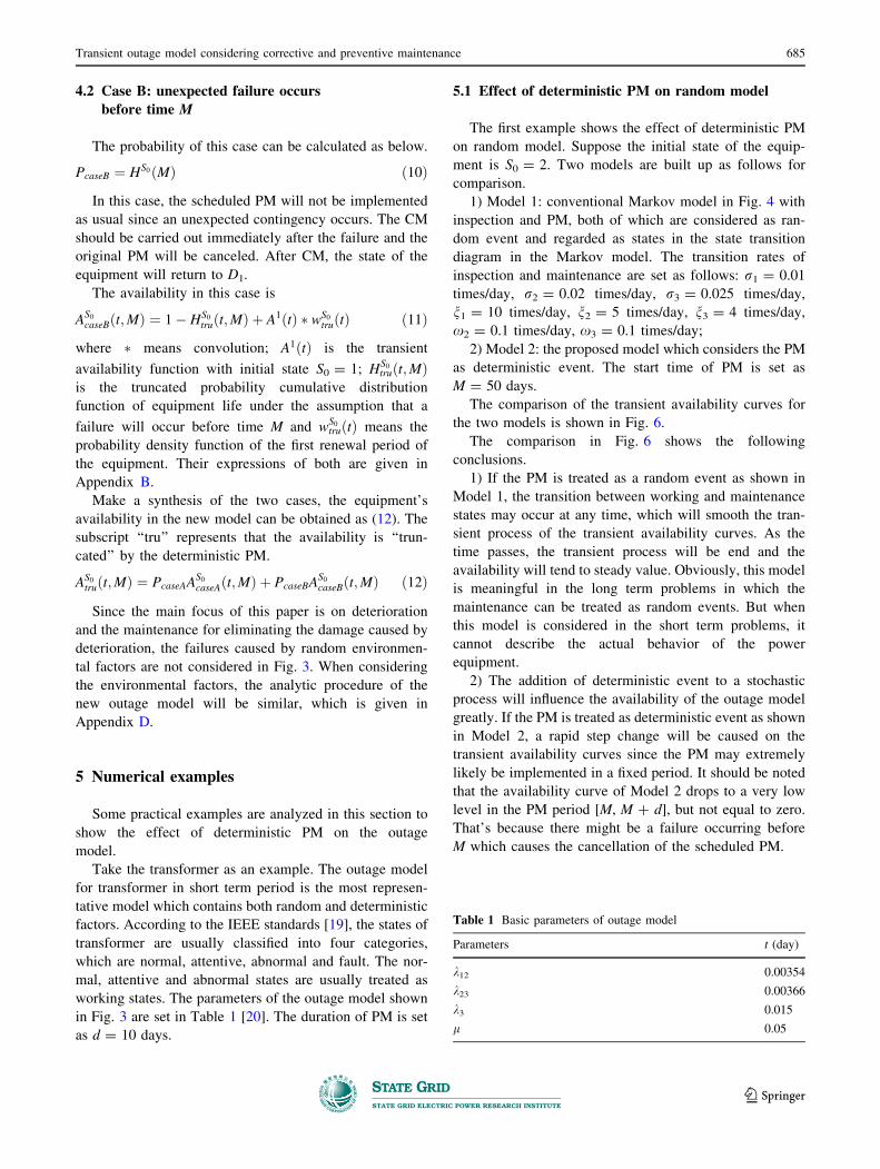
working states. The parameters of the outage model shown
in Fig. 3 are set in Table 1 [20]. The duration of PM is set
as d = 10 days.
5.1 Effect of deterministic PM on random model
The first example shows the effect of deterministic PM
on random model. Suppose the initial state of the equip-
ment is S0 = 2. Two models are built up as follows for
comparison.
1) Model 1: conventional Markov model in Fig. 4 with
inspection and PM, both of which are considered as ran-
dom event and regarded as states in the state transition
diagram in the Markov model. The transition rates of
inspection and maintenance are set as follows: r1 = 0.01
times/day, r2 = 0.02 times/day, r3 = 0.025 times/day,
n1 = 10 times/day, n2 = 5 times/day, n3 = 4 times/day,
x2 = 0.1 times/day, x3 = 0.1 times/day;
2) Model 2: the proposed model which considers the PM
as deterministic event. The start time of PM is set as
M = 50 days.
The comparison of the transient availability curves for
the two models is shown in Fig. 6.
The comparison in Fig. 6 shows the following
conclusions.
1) If the PM is treated as a random event as shown in
Model 1, the transition between working and maintenance
states may occur at any time, which will smooth the tran-
sient process of the transient availability curves. As the
time passes, the transient process will be end and the
availability will tend to steady value. Obviously, this model
is meaningful in the long term problems in which the
maintenance can be treated as random events. But when
this model is considered in the short term problems, it
cannot describe the actual behavior of the power
equipment.
2) The addition of deterministic event to a stochastic
process will influence the availability of the outage model
greatly. If the PM is treated as deterministic event as shown
in Model 2, a rapid step change will be caused on the
transient availability curves since the PM may extremely
likely be implemented in a fixed period. It should be noted
that the availability curve of Model 2 drops to a very low
level in the PM period [M, M ? d], but not equal to zero.
That’s because there might be a failure occurring before
M which causes the cancellation of the scheduled PM.
Table 1 Basic parameters of outage model
Parameters t (day)
k12 0.00354
k23 0.00366
k3 0.015
l 0.05
Transient outage model considering corrective and preventive maintenance 685
123

3) The transient availability curve of Model 2 is much
closer to the real situation in the short term since it reflects
the deterministic factors which actually exist in the real
world. Meanwhile, the conventional Markov model is not
suitable for the short-term maintenance schedule problem
in which random and deterministic factors coexist together.
5.2 Availability with different initial state
The equipments with PM are usually the ones operating
in inferior states. Three models are built up to show the
impact of the initial states on the transient availability
curves.
1) Model 1: the proposed model which considers the PM
as deterministic event. The start time of PM is set as
M = 50 days and the initial state is S0 = 1, which is nor-
mal state;
2) Model 2: the same as Model 1 except that the initial
state is S0 = 2, which is attentive state;
3) Model 3: the same as Model 1 except that the initial
state is S0 = 3, which is abnormal state.
The transient availability curves of the three models are
shown in Fig. 7.
Figure 7 demonstrates the impact of different initial
states on the transient availability curves. If the initial state
of equipment is normal, the availability is very close to 1
and the unexpected failure can hardly occur. If inspection
result shows that the equipment operating in a very inferior
state, such as in 3, the probability that a failure occurs
unexpectedly before the scheduled PM will be much larger,
which means the PM may very likely be canceled. For the
transient availability curve of Model 3, the maximal
unavailability in the next few days is nearly 0.2 and the
probability that the PM is carried out as usual is only about
0.6. Therefore, it is clear that the equipment with worse
working condition should be paid more attention and the
PM on these equipments cannot be scheduled too late.
6 Conclusion
In the problems of short-term maintenance schedule,
both random and deterministic factors may coexist together
and the transient state probability of equipment should be
considered. This paper mainly focuses on the outage model
used in the short-term problems and a Markov-based
transient outage model is proposed, considering the effect
of both random CM and deterministic PM. The transient
availability function of the outage model is presented and
special emphasis is made on the impact of an unexpected
failure occurring prior to PM. The results demonstrate that
the addition of deterministic PM significantly influences
the transient availability of the equipment.
The research discussed in this paper provides a new
viewpoint on the outage model used in short-term prob-
lems. The model considering the effect of random and
deterministic events is applicable to a more extensive field.
Future work will focus on the model application in the risk
assessment and short term maintenance schedule opti-
mization in the power systems.
Acknowledgements This work was supported by the Key Tech-
nologies Research and Development Program of China (No.
2013BAA01B03), the National Natural Science Foundation of China
(No. 51177080, No. 51321005), and the Program for New Century
Excellence Talents in University (No. NCET-11-0281).
Open Access This article is distributed under the terms of the
Creative Commons Attribution 4.0 International License (http://
creativecommons.org/licenses/by/4.0/), which permits unrestricted
use, distribution, and reproduction in any medium, provided you give
appropriate credit to the original author(s) and the source, provide a
link to the Creative Commons license, and indicate if changes were
made.
0 10 20 30 40 50 60 70 80 90 100
0.1
0.2
0.3
0.4
0.5
0.6
0.7
0.8
0.9
1.0
t (day)
Ava
ilabi
lity
Model 1 Model 2
Fig. 6 Transient availability curves of Model 1 and Model 2
0 10 20 30 40 50 60 70 80 90 100
0.1
0.2
0.3
0.4
0.5
0.6
0.7
0.8
0.9
1.0
t (day)
Ava
ilabi
lity
Model 1 Model 2 Model 3
Fig. 7 Availability curves with different initial state
686 Guoqiang JI et al.
123

Appendix A
Equation (5) can be rewritten as follows:
dP1 tð Þdt
¼ �k12P1 tð Þ þ lPNþ1 tð ÞdP2 tð Þdt
¼ k12P1 tð Þ � k23P2 tð Þ
..
.
dPNþ1 tð Þdt
¼ kNPN tð Þ � lPNþ1 tð Þ
8>>>>>>>><
>>>>>>>>:
ðA1Þ
Suppose the initial state of the equipment is S0. The time
domain (A1) can be change into (A2) through Laplace
transformation.
sP1 ¼ �k12P1 þ lPNþ1
sP2 ¼ k12P1 � k23P2
..
.
sPS0 � 1 ¼ kS0�1;S0PS0�1 � kS0;S0þ1PS0
..
.
sPNþ1 ¼ kNPN � lPNþ1
8>>>>>>>><
>>>>>>>>:
ðA2Þ
The analytical expression of each state probability can
be obtained by solving the algebraic (A2). The basic form
of the expression of Pk (k = 1, 2,���, N ? 1) is as (A3). The
superscript S0 means the initial state of the equipment.
PS0k ¼ Pk1
sþXN
i¼1
Lkisþ si
; k ¼ 1; 2; � � � ; N þ 1 ðA3Þ
The time domain expression of Pk can be obtained
through inverse Laplace transformation as shown in (2).
The solution procedure of the case with other initial state
will be similar.
Appendix B
Define the equipment natural life as the period from the
current time to the time when an unexpected failure occurs.
The probability cumulative distribution function H(t) in (8)
means the probability that a failure occurs before time t in
the natural deterioration process, given the premise that the
equipment is working at initial time. Based on the defini-
tion, the differential equations can be listed as follows:
dP
dt¼ P
�k12 k12. .. . .
.
�kN�1;N kN�1;N
�kN kN0 � � � 0
2
666664
3
777775
P ¼ P1 tð Þ P2 tð Þ � � � PN tð Þ H tð Þ½ �
8>>>>>>><
>>>>>>>:
ðB1Þ
Noticed that the last row of the matrix in the right hand
equals to 0 because it is supposed that all the repair rates lequal to 0 when calculating the probability cumulative
distribution function of equipment natural life. Suppose the
initial state of equipment is S0. The function HS0 tð Þ can be
obtained by solving (B1).
Based on HS0 tð Þ, the probability density function of
equipment life can be given as follows:
hS0 tð Þ ¼ dHS0 tð Þdt
ðB2Þ
According to the expression (B2), the failure may occur
on the equipment at any time. However, if it is assumed
that a failure will occur before time M, obviously the
probability density function will equal to 0 in the period
[M, ??]. The new density function can be called
‘‘truncated’’ probability density function and the
expression is as follows:
hS0tru t;Mð Þ ¼hS0 tð Þ
1�Rþ1M
hS0 uð Þdu; t 2 0;M½ Þ
0; t 2 M;þ1½ Þ
8<
:ðB3Þ
The truncated probability cumulative distribution
function of the equipment life can be obtained as follows:
HS0tru t;Mð Þ ¼
HS0 tð Þ1�
Rþ1M
hS0 uð Þdu; t 2 0;M½ Þ
1; t 2 M;þ1½ Þ
8<
:ðB4Þ
The probability cumulative distribution function of the
repair time is an exponential distribution, since the repair
rate is assumed to be constant. Hence the probability
density function of repair time with repair rate l is as
follows:
g tð Þ ¼ le�lt ðB5Þ
The probability density function of renewal period
(summation of equipment natural life and repair time) can
be calculated via convolution:
wS0 tð Þ ¼ hS0 tð Þ � g tð ÞwS0tru t;Mð Þ ¼ hS0tru t;Mð Þ � g tð Þ
�
ðB6Þ
Appendix C
Suppose the equipment keeps working during the period
[0, M] and the initial state is S0, the conditional probability
of equipment at state k during [0, M] can be calculated as
follows:
PS0conk tð Þ ¼ PS0
k tð ÞAS0 tð Þ ; k ¼ 1; 2; � � � ;N; 0� t�M ðC1Þ
Transient outage model considering corrective and preventive maintenance 687
123

It is assumed that after PM the equipment will return to
the previous state by one stage. If the equipment is in 1 at
time t = M, after PM it will return to 1 again. So the
relationship between state probability of the equipment
after PM and before PM can be expressed as follows:
PS0SMþd
¼ PS0conSM
Mð Þ
SMþd ¼
1; SM ¼ 1; 22; SM ¼ 3
..
.
N � 1; SM ¼ N
8>>><
>>>:
8>>>>><
>>>>>:
ðC2Þ
Appendix D
When considering the random environmental factors,
the outage model in Fig. 3 can be modified to Fig. D1 as
below.
The states F1 * FN represent the failure state caused by
random environmental factors. ~kk and ~lk mean the corre-
sponding failure rate and repair rate. When the failure
caused by random environmental factors occurs, the
equipment will be repaired and return to operation after
repair. Since the failure is not caused by the deterioration,
it is assumed that the intent of the corresponding repair is
just the re-establishment of the working state and the
equipment will return to the state which is the one just
before failure. Obviously this assumption can also be easily
relaxed. The equations of the model in Fig. D1 are shown
as (D1).
Equation (D1) can also be solve through Laplace
transformation and the time domain expression of each
state probability is similar to (6) with 2 N exponential
terms.
When the deterministic PM is added to the outage model
in Fig. D1, the analysis procedure is similar to the proce-
dure mentioned above. Special attentions need to be paid
on the following points:
1) The definition of equipment natural life in this case is
different from the one mentioned above. Define the
equipment natural life as the period from the current time
to the time when a failure caused by deterioration occurs. It
should be noted that the failure caused by random envi-
ronmental factors is not regarded as the end of the equip-
ment’s life. Therefore, the probability cumulative
distribution function H(t) equals to PN?1(t) in the case that
l = 0 in (D1).
2) Typically, the severity of the failure caused by ran-
dom environmental factors is much lighter that the failure
caused by deterioration and the repair time of failure
caused by random environmental factors will be much
shorter as well. Therefore, it is supposed that if a failure
caused by random environmental factors occurs before M,
the equipment will return to operation after repair and the
original PM will be carried out as usual. Only the occur-
rence of failure caused by deterioration during the period
[0, M] can cause the cancellation of PM and the immediate
implementation of CM.
212λk k+1, 1k kλ + N+1N
Nλ
μ
F1 F2 Fk Fk+1 FN
1λ 1μ 2λ 2μkλ kμ 1kλ + 1kμ + Nλ Nμ
1
Fig. D1 Markov-based equipment outage model considering the
failure caused by random environmental factors
dP
dt¼ P
� k12 þ ~k1� �
k12 � � � ~k1
� k23 þ ~k2� �
k23 � � � . ..
..
. ... . .
. . .. . .
.
� kN�1;N þ ~kN�1
� �kN�1;N
. ..
� kN þ ~kN� �
kN ~kNl �l~l1 �~l1
. .. . .
. . .. . .
.
~lN �~lN
2
66666666666666666664
3
77777777777777777775
P ¼ PD1 tð Þ � � � PDN tð Þ PF tð Þ PF1 tð Þ � � � PFN tð Þ½ �
8>>>>>>>>>>>>>>>>>>>>><
>>>>>>>>>>>>>>>>>>>>>:
ðD1Þ
688 Guoqiang JI et al.
123

References
[1] Li WY (2005) Risk assessment of power systems: models,
methods, and applications. Wiley, Hoboken, NJ, USA
[2] Ross SM (1996) Stochastic processes, 2nd edn. Wiley, New
York, NY, USA
[3] Endrenyi J, Aboresheid S, Allan RN et al (2001) The present
status of maintenance strategies and the impact of maintenance
on reliability. IEEE Trans Power Syst 16(4):638–646
[4] Billinton R, Allan RN (1996) Reliability evaluation of power
systems. Springer, Boston, MA, USA
[5] Makis V, Jardine AKS (1992) Optimal replacement policy for a
general model with imperfect repair. J Oper Res Soc
42(2):111–120
[6] Kuntz PA, Christie RD, Venkata SS (2001) A reliability cen-
tered optimal visual inspection model for distribution feeders.
IEEE Tran Power Deliver 16(4):718–723
[7] Endrenyi J, Anders GJ, Leite da Silva AM (1998) Probabilistic
evaluation of the effect of maintenance on reliability: an appli-
cation. IEEE Trans Power Syst 13(2):576–583
[8] Sim SH, Endrenyi J (1993) A failure-repair model with minimal
and major maintenance. IEEE Trans Reliab 42(1):134–140
[9] Agepati R, Gundala N, Amari SV (2013) Optimal software
rejuvenation policies. In: Proceedings of the 60th annual relia-
bility and maintainability symposium (RAMS’13), Orlando, FL,
USA, 28–31 Jan 2013, 7 pp
[10] Amari SV, McLaughlin L, Pham H (2006) Cost-effective con-
dition-based maintenance using Markov decision processes. In:
Proceedings of the 52nd annual reliability and maintainability
symposium (RAMS’06), Newport Beach, CA, USA, 23–26 Jan
2006, pp 464–469
[11] Amari SV, McLaughlin L (2004) Optimal design of a condition-
based maintenance model. In: Proceedings of the 50th annual
reliability and maintainability symposium (RAMS’04), Los
Angeles, CA, USA, 26–29 Jan 2004, pp 528–533
[12] Welte TM (2009) Using state diagrams for modeling mainte-
nance of deteriorating systems. IEEE Trans Power Syst
24(1):58–66
[13] Abeygunawardane SK, Jirutitijaroen P (2011) New state dia-
grams for probabilistic maintenance models. IEEE Trans Power
Syst 26(4):2207–2213
[14] Kijima M, Sumita U (1986) A useful generalization of renewal
theory: counting processes governed by non-negative Markovian
increments. J Appl Probab 23(1):71–88
[15] Kijima M (1989) Some results for repairable systems with
general repair. J Appl Probab 26(1):89–102
[16] Yuan FQ, Kumar U (2012) A general imperfect repair model
considering time-dependent repair effectiveness. IEEE Trans
Reliab 61(1):95–100
[17] Nakagawa T (1979) Optimum policies when preventive main-
tenance is imperfect. IEEE Trans Reliab 28(4):331–332
[18] Wu SM, Clements-Croome D (2005) Optimal maintenance
policies under different operational schedules. IEEE Trans
Reliab 54(2):338–346
[19] IEEE Std C57.104 2008. IEEE guide for the interpretation of
gases generated in oil-immersed transformers. 2009
[20] Pathak J, Jiang Y, Honavar V, et al (2006) Condition data
aggregation with application to failure rate calculation of power
transformers. In: Proceedings of the 39th annual Hawaii inter-
national conference on system sciences (HICSS’06), Vol 10,
Kauai, HI, USA, 4–7 Jan 2006, pp 241–251
Guoqiang JI received the B.S., and Ph.D. degrees all from electrical
engineering, Tsinghua University, Beijing. His research interest is
power system risk assessment and maintenance scheduling.
Wenchuan WU received the B.S., M.S. and Ph.D. degrees all from
the Electrical Engineering Department, Tsinghua University, China.
Currently, he is a full professor in the Department of Electrical
Engineering of Tsinghua University. His research interests include
Energy Management System, active distribution system operation and
control, and EMT-TSA hybrid real-time simulation. He is an
associate editor of IET Generation, Transmission & Distribution
and associate editor of Electric Power Components and Systems.
Boming ZHANG received his Ph.D. degree from Tsinghua Univer-
sity, Beijing, China, in 1985, in electrical engineering. Since then, he
was appointed as a lecturer, associate professor and full professor in
the Department of Electrical Engineering of Tsinghua University. His
research interests include power system analysis and control,
especially on the EMS advanced applications for EPCC.
Hongbin SUN received his Ph.D. degree from Tsinghua University,
Beijing, China, in 1997 in electrical engineering. Currently, he is a
full professor in the Department of Electrical Engineering of
Tsinghua University. His research interests focus on the power
system analysis and control, especially on automatic voltage control.
Transient outage model considering corrective and preventive maintenance 689
123