Transmission Line Fault Location Explained

Transmission Line Fault Location Explained Page 1 of 12

Transmission Line Fault Location Explained

A review of single ended impedance based fault location methods, with real life examples

Presented at the

2018 Georgia Tech Fault and Disturbance Analysis Conference

Robert Orndorff, Kyle Thomas, Patrick Hawks, Brian Starling Dominion Energy

Amir Makki, Maria Rothweiler

SoftStuf Dominion Energy has spent several years implementing automated fault location algorithms on our system events, and over that time we have become familiar with the various available fault location methods. We have come to understand these formulas and want to share what we have learned. Many people are intimidated by the formulas used to calculate fault locations. The intent of this paper is to step through the math involved in calculating fault locations from DFR or relay data and simplify it in a way that is easy to understand. In this paper, we will cover the simple single end impedance based fault location methods. The math involved is relatively easy to do with a handheld calculator. By stepping through the calculations we intend to give the reader better insight into the data that goes into the resulting locations. Once you understand these simple methods, the lessons learned can be used to understand the more complex methods used to achieve even better accuracy. This paper will step through examples using real fault data for each fault type. The simplest, mathematically speaking, are phase to phase faults, so we begin with that example, followed by three phase, and finally we go through a phase to ground example.


Phase to Phase faults IEEE C37.114 lists the simple methods available for single ended fault location. Perhaps the easiest to understand is the formula for a phase to phase, or line to line, fault. Consider the diagram below (Figure 1) with a source, load, and two lengths of wire connecting them.

Under normal conditions the source sees 20 ohms of resistance plus the resistance of the load. Now suppose there is a fault (short circuit) bridging the two wires at 60% of the length of the wire (Figure 2).

In this case the source now sees 6Ω + 6Ω of resistance for 12 ohms total. Also assume we measure voltage and current at the source, the equivalent of a smart relay or Digital Fault Recorder (DFR). For this fault we would measure 100 volts and 8.33 amps, which results in a resistance of 12 ohms. Since the total resistance of the circuit is 20 ohms, the distance to fault calculation would be determined as follows: Comparing the measured resistance to the already known total resistance will result in a percent distance to fault, assuming that the resistance is the same along the entire length of the line.

Source 100 V

6 Ω

6 Ω

Source 100 V

10 Ω

10 Ω

Figure 1 – Simple

circuit with a source,

load, and two lengths

of wire.

Figure 2 – Phase to

phase fault 60%

down line from the

source.


At this point it is a simple matter to multiply the line length by the percentage given by the equation to get the physical distance to the fault. Now let’s look at the equation given in the IEEE C37.114 for a phase to phase fault. In this case it will be a fault between A and B phases.

This gives impedance to the fault location, assuming the fault itself has zero (or negligible) impedance. Compare this measured impedance to the total impedance to get a calculated fault location. Vab is defined as Va-Vb and Iab is defined as Ia-Ib. In the example above the voltage is 100-0, or 100 volts and the current would actually be twice the loop current because we are subtracting the out of phase return current from the outgoing phase current.

Note that because we effectively doubled the current in the equation, we cut the impedance in half. Instead of 12 ohms, we got an answer of 6 ohms. This is method is convenient in that it doesn’t require we count the impedance of both outgoing and return current paths. We just use the impedance of a single wire to calculate location. In this case the calculation is 6 ohms divided by 10 ohms, which gives us the correct answer of 60% of total line length. One advantage that does exist in using both the outgoing and return current is that we can take into account real world unbalance that exists in the impedances and load flows on each phase. It isn’t, however, mandatory for a decent location. Up to this point we have been using simple circuits using only DC resistance. Since the power system is AC and has resistance and reactance, you use the same formulas but plug in the complex values of voltages and currents. Here is a real world example of a phase to phase fault, complete with the calculations shown. The fault recorder data for a fault on a 230kV transmission line is shown below in Figure 3. The values are derived from one cycle of data between the solid vertical bar and the preceding dotted vertical bar.


Given the following line data and using the recorded values shown in Figure 3.

In this case 14.25 miles is the correct answer. Note that the fault location result includes an angle. Normally the field crews do not expect an angle to be given with the mileage, so we should determine if the angle is meaningful. Since the distance to the fault should simply be a magnitude, we expect that the angle of the result should be close to zero. In this case it is very close to zero and can be ignored. If the angle gets very large, there may be an error in the calculation or errors in the data. We use a rule of thumb of about ±15 degrees as a guide as to when the location calculation may be less accurate. If the angle is within 15 degrees of zero, it’s likely a good result, however more research is needed in this area. Reactance IEEE C37.114 lists the simple reactance method, which is similar to the calculations shown above, except that only the reactive portion of the numbers are used when calculating the per

Figure 3 – DFR

Measurements from a

phase to phase fault.


unit distance to fault. By using only the reactance, any errors due to resistance of the fault are reduced. However, when fault resistance becomes too high, the reactance method does not provide reliable results. In our calculations, we would convert the polar form of the numbers to rectangular in order to find the reactance portion of the values.

In this case the reactance method yields the same answer you get by using the simple impedance method. The reactance phase to phase method can also be used for phase to phase to ground faults. It even gives reasonable results for three phase faults. Three phase faults Distance to fault calculations for three phase faults can be made using the same methods used for phase to phase faults. Choose two of the three phases and perform the calculations as shown above. A slightly more accurate method, however, would be to simply use the positive sequence voltage and current values.

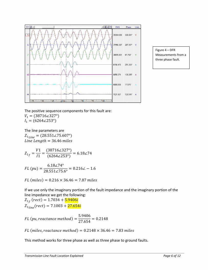
Here is an example of a real three phase fault with DFR measurements. The line had a three phase fault 7.92 miles from the substation. The values recorded by the DFR are shown below.


The positive sequence components for this fault are: The line parameters are

If we use only the imaginary portion of the fault impedance and the imaginary portion of the line impedance we get the following:

This method works for three phase as well as three phase to ground faults.

Figure 4 – DFR

Measurements from a

three phase fault.


Phase to ground faults

Phase to ground faults are fundamentally different from phase only faults in that the

return path taken by the ground or zero sequence current has a different impedance

(being an entirely distinct and parallel path) than the line phase conductor. Again, the

voltage and currents are measured at the source. The formula for finding the positive

sequence fault impedance for an A phase to ground fault, according to C37-114 is:

The k (or k0) factor introduced in this formula is called the zero sequence compensation factor. The k factor is applied to the neutral current in the impedance calculation. This results in an impedance that is relative to the positive sequence impedance of the line. The formula for calculating the k factor is shown below.

Where Fault location is then determined by


Figure 5 shows phase to ground fault data from a DFR for a fault located 10.2 miles from the station.

First, calculate k0.

Now, calculate measured impedance for this C phase to ground fault.

Using reactance only yields the following

Figure 5 – DFR

Measurements from a

phase to ground fault.


In this case, the reactance method results in a slightly more accurate location. It’s not a simple task to directly illustrate the k0 factor using a simple DC circuit. The k0 factor is derived from a combination of mutual impedance of all three phase conductors as well as the self-impedance of the conductors. Some descriptions of the k0 factor indicate that it was derived to compensate for the difference between the positive and zero sequence impedances. While this is true, it’s not a complete description. One thing to consider when taking measurements to be used in these formulas is where in the fault the measurements should be taken. In a previous paper, we tried various cursor placements to see if there was an impact on fault location accuracy. We found that most of the time using a window between 0.75 and 1.75 cycles into the fault provides good results. This allows time for the fault currents and voltages to stabilize. Note that when the math is done on these calculations, the result also includes an angle, with the exception of the reactance only methods. Ideally this angle should be close to zero since fault location is a simple scalar value. In the examples shown in this paper the result angle is less than 3 degrees. For phase to ground faults where the angle between the voltage and current is significantly less than the line angle, the fault is often a high impedance fault. Typical angle values for our transmission lines are between 70 and 80 degrees. We have found we are less likely to get accurate results on faults where the angle between the faulted phase voltage and current is less than 40 degrees. In this case, algorithms that performs better with high impedance faults should be considered. Compensating for load In the examples shown so far we have used either ideal values or values recorded during the fault. The fault values do not take into account the effect of load on the measured fault values. By using the imaginary, or reactive, portion of the data, the effect of load is reduced. Several, more advanced, algorithms do take load into consideration in an effort to obtain more accurate results. Some of these do so by measuring the pre-fault load values, particularly current values, and subtracting them from the mid-fault values to isolate current generated by the fault. In doing so, the formulas are now working with the change in current created by the fault, thereby resulting in a more accurate fault location.


Calculating Fault Impedance Once the actual fault location is known, then it should be possible to calculate the actual impedance of the fault. The formulas and algorithms discussed in this paper assume that the fault impedance is zero. Therefore if you obtain an accurate fault location using these methods, it’s safe to assume that the impedance of the fault is relatively close to zero. However, if the calculated and actual locations are different then the problem could be that there was a non-zero fault impedance, or that there are errors in the line data. In the case of phase to ground faults, the sources of error are usually inaccurate zero sequence impedance model data or high fault impedance. While it should be possible to calculate the zero sequence impedance for a phase to ground fault, given the fault location, it’s not a simple task. The difficulty lies in the fact that in order to calculate the measured fault impedance you must use the k0 factor. The k0 factor includes the zero sequence impedance, which is the quantity that you are trying to solve for. This is a topic for future discussion. At Dominion Energy, we have automated processes calculating fault location using the reactance methods discussed in this paper. We have been collecting statistics on the accuracy of these calculated locations. A summary of the fault locations is shown in Table 1. This table shows only locations generated by the reactance methods outlined in this paper. Our automation also gathers fault locations from relays, DFRs, traveling wave locators, and system models as well as double ended location calculations if enough information is available. The impedance based reactance method is one part of all the data that is presented by the automation. When multiple methods agree on a location, then it gives good confidence in the results.

Fault type Operations Average error (miles) Median error (miles) Phase to ground 109 1.32 0.45

Phase to phase and PPG 25 1.30 0.48

Three phase and 3PG 11 2.91 0.95

Table 1 – Reactance method fault locations Conclusions The basic fault location algorithms are not too difficult to understand once the steps are explained and you work through them manually. All of the examples in this paper are using data from real faults and only a handheld calculator was used to perform the math. The intent was to walk through the calculations and allow for a better understanding of how the locations are calculated. Once you understand the algorithms, you are in a better position to look for sources of error and improve on the results. One single method of fault location by itself is good, but multiple methods combined give a much better indication of the actual fault location. By comparing results from single ended impedance based methods, double ended methods, traveling wave, and lightning correlation you can get a very good idea of the confidence of the accuracy of the locations provided.


References Three-Phase Circuit Analysis and the Mysterious k0 Factor S. E. Zocholl Schweitzer Engineering Laboratories, Inc., 1995 IEEE Guide for Determining Fault Location on AC Transmission and Distribution Lines IEEE C37.114-2004 IEEE Power Engineering Society Ground Distance Relays – Understanding the Various Methods of Residual Compensation, Setting the Resistive Reach of Polygon Characteristics, and Ways of Modeling and Testing the Relay Quintin Verzosa, Jr. “Jun” Doble Engineering Company Observations on the Application of the IEEE C37.114 Double Ended Fault Location Method Hawks, Makki, Orndorff, Rothweiler ,Starling, Thomas Dominion Energy, SoftStuf


Biographies

Patrick Hawks has worked at Dominion Virginia Power since 2008. He has a B.S. degree in Computer Engineering from Virginia Commonwealth University. His experience includes six years in system protection, wherein he participated in system modeling, relay settings, and protection standard development, implementing a substantial degree of automation, both in setting calculation and setfile generation. He has since moved into Fault Analysis and become involved in analyzing system events and web app development. Amir Makki has worked at Softstuf since 1991. He has BS and MS degrees in Electrical Engineering from Tennessee Tech University and pursued his Ph.D. studies in Software Engineering at Temple University. His main interest is automating fault and disturbance data analysis. He is extensively published and holds a number of U.S. patents and trademarks. Amir is a senior member of IEEE and is an active member of the Protection Systems Relay Committee where he chaired a number of working groups including COMTRADE, COMNAME, and the Cyber Security Task Force for Protection Related Data Files.

Robert Orndorff has worked at Dominion Virginia Power since 1984. He earned an A.A.S degree in Electronics in 1986 and spent 11 years as a field relay technician and in 1997 transferred to the Fault Analysis department where he currently works. His current responsibilities include maintaining and configuring Dominion’s Digital fault recorders, event retrieval and analysis from smart relays and DFRs. Robert is an IEEE member and has been a member of the Transient Recorder’s User Council (TRUC) since 2002.

Maria Rothweiler has worked at Softstuf since 1991. She has a Bachelor of Arts degree in Computer Science from Temple University and pursued her associate degree in Mathematics at Bucks County Community College. Her main interest is developing software tools for display and analysis of power system fault and disturbance data. She is extensively published and holds a number of U.S. patents, trademarks, and copyrights. Maria is a member of IEEE and an active member of the IEEE Standards Association.

James B. Starling has worked at Dominion Virginia Power since 2003. He has a BS degree in Electrical Engineering from Virginia Commonwealth University. His experience includes testing, installing, and repairing relay systems and calculating line impedances and relay settings. He also has extensive experience analyzing and documenting transmission system operations. He is currently responsible for compliance reporting, misoperation investigations, and fault recorders. Brian is a Master Black Belt Six Sigma for helping reduced Dominion’s transmission operations by 22%.

Kyle Thomas received his M.S. degree in Electrical Engineering from Virginia Tech in 2011 and is currently pursuing his Ph.D. while working for Dominion Virginia Power’s Electric Transmission Operations Research group. He has technical expertise in power system protection/control, wide-area measurements, fault analysis, cascading analysis/physical security, and system simulations. Kyle is a technical lead of Dominion’s synchrophasor installations, applications, and training, and is actively involved in the North American Synchrophasor Initiative (NASPI), IEEE, and CIGRE organizations.

Documents

Transmission Line Fault Location Explained