Embed Size (px)
DESCRIPTION
Operations Research
Citation preview
1
CHAPTER 7
Transportation Problem
7.1 Introduction
The transportation problem is one of the subclasses of LPPs in which the objective is to transport various
quantities of a single homogeneous commodity that are initially stored at various origins to different
destinations in such a way that the transportation cost is minimum. To achieve this objective we must
know the amount and location of available supplies and the quantities demanded. In addition we must
known the costs that result from transporting one unit of commodity from various origins to various
destinations.
Let
m be the number of sources
n be the number of destinations
ai be the supply at the source i
bj be the demand at the destination j
cij be the cost of transportation per unit from source i to destination j
Xij be the number of units to be transported from the source i to the destination j. The Linear
programming model representing the transportation problem is given by
Minimize ∑∑= =
=m
1i
n
1jijijXCZ
subject to the constraints
m....3,2,1i,aXn
1jijij =≤∑
=
(Row Sum) and
n....3,2,1j,bXm
1iijij =≥∑
=
(Column Sum)
0Xij ≥ for all i and j
The objective function minimizes the total cost of transportation (z) between various sources and
destinations. The constraint i in the first set of constraints ensures that the total units transported from the
source i is less than or equal to its supply. The constraint j in the second set of constraints ensures that the
total units transported to the destination j is greater than or equal to its demand.

2
Fig. 7.1 Schematic Diagram of Simple Transportation
Example 3.1 Consider the following transportation problem (Table 3.3) involving 3 sources and 3
destinations. Develop a linear programming (LP) model for this problem and solve it.
The given transportation problem is said to be balanced if
∑∑==
=n
1jj
m
1ii ba
ie. if the total supply is equal to the total demand.
This restriction causes one of the constraints to be redundant (and hence it can be deleted) so that the
problem will have (m + n – 1) constraints and (m x n) unknowns.
Note that a transportation problem will have a feasible solution only if the above restriction is satisfied.
Thus, ∑∑==
=n
1jj
m
1ii ba is necessary as well as a sufficient condition for a transportation problem to have a
3
feasible solution. Problems that satisfy this condition are called balanced transportation problems.
Techniques have been developed for solving balanced or standard transportation problems only. It
follows that any non-standard problem in which the supplies and demands do not balance, must be
converted to a standard transportation problem before it can be solved. This conversion can be achieved
by the use of a dummy source/destination.
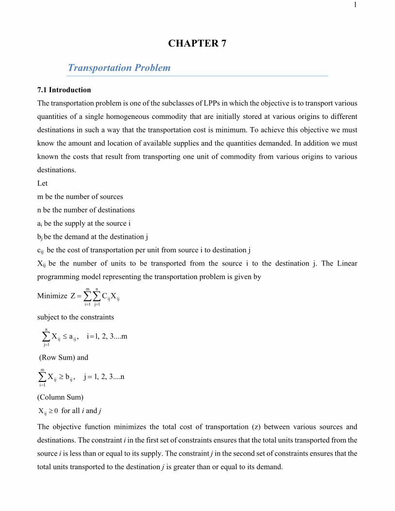
The above information can be put in the form of a general matrix shown below:
TABLE 7.1 Cost Matrix of Transportation Problem
Definitions
A few terms in connection with Transportation model are defined below
Feasible Solution Any set of non negative allocations ( 0Xij > ) which satisfies the row and column sum
(rim requirement) is called a feasible solution.
Basic Feasible Solution A feasible solution is called a basic feasible solution if the number of non
negative allocations is equal to m+n-1 here m is the number of rows, n is the number of columns in a
transportation table.
Non-degenerate Basic Feasible Solution
Any feasible solution to a transportation problem containing in origins and n destinations is said to be
non-degenerate, if it contains m+n-1 occupied cells and each allocation is in independent positions.
The allocations are said to be in independent positions, if it is impossible to form a closed path.
Closed path means by allowing horizontal and vertical lines and all the corner cells are occupied.

4
Optimal Solution A feasible solution that minimizes (maximizes) that the transportation cost (profit) is
called an optimal solution. The solution of a transportation problem. can be obtained in two stages,
namely initial solution and optimal solution. Initial solution can be obtained by using any one-of the
three methods
(i) North west corner rule (NWCR)
(ii) Least cost method or Matrix minima method(LCM)
(iii) Vogel's approximation method (VAM)
VAM is preferred-over the other two methods, since the initial basic feasible solution obtained by this
method is either optimal or very close to the optimal solution.
The cells in the transportation table can be classified as occupied cells and unoccupied cells. The
allocated cells in the transportation table is called occupied cells and empty cells in a transportation table
is called unoccupied cells.
The improved solution of the initial basic feasible solution is called optimal solution which is, the
second stage of solution that can be obtained by MODI (modified distribution method).
The allocations in the following tables are not in independent positions.
The allocations in the following tables are in independent positions.
TABLE 7.2 Allocation of Different Possible Ways of Items
* *
* *
* *
* *
* *
* *
*
* *
* *
* *
5
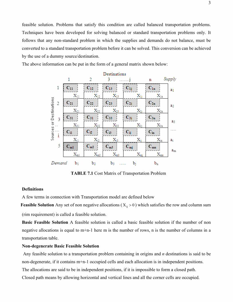
Degenerate Basic Feasible Solution If a basic feasible solution contains less than m+n-1 non negative
allocations, it is said to be degenerate.
Example 7.1 Consider the following transportation problem (Table 7.3) involving 3 sources and 3
destinations. Develop a linear programming (LP) model for this problem and solve it
Table 7.3 Example 7.1
Solution Let Xij be the number of units to be transported from the source i to the destination j, where i =
1, 2, 3 and j = 1, 2, 3. An LP model of this problem is:
333231232221311211 X9X7X3X8X2X6X8X5X4ZMinimize ++++++++=
subject to
.3,2,1jand3,2,1i,0X100XXX200XXX200XXX200XXX200XXX
100XXX
ij
332313
322212
312111
333231
232221
311211
==≥≥++≥++≥++≤++≤++≤++
Application of simplex method to the above LP model yields the optimal shipping plan as presented
in Table 7.4.
Table 3.4 Optimal Shipping Plan (Example 3.1)
6
Source Destination Quantity shipped
1 3 100
2 2 200
3 1 200
Total minimum cost = Rs. 1800
7.2 TYPES OF TRANSPORTATION PROBLEM
The transportation problem can be classified into balanced transportation problem and unbalanced
transportation problem.
7.2.1 Balanced Transportation Problem
If the sum of the supplies of all the sources is equal to the sum of the demands of all the destinations, then
the problem is termed as balanced transportation problem. This may be represented by the relation:
∑∑==
=n
1jj
m
1ii ba
Example 3.1 represents a balanced transportation problem.
7.2.2 Unbalanced Transportation Problem
It is the sum of the supplies of all the sources is not equal to sum of the demands of all the destinations,
then the problem is termed as unbalanced transportation problem. That means, for any unbalanced
transportation problem, we have
∑∑==
≠n
1jj
m
1ii ba
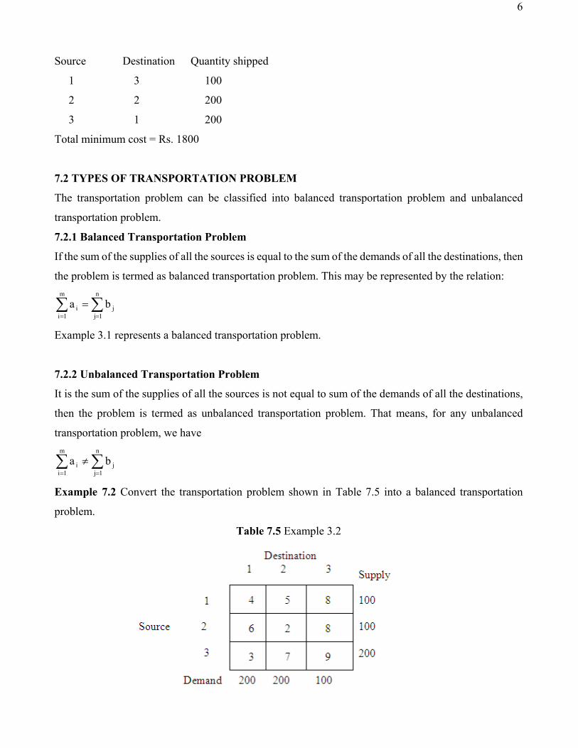
Example 7.2 Convert the transportation problem shown in Table 7.5 into a balanced transportation
problem.
Table 7.5 Example 3.2
7
Solution For the given problem,
500band,400an
1jj
m
1ii == ∑∑
==
Here, ∑∑==
≠n
1jj
m
1ii ba
Hence it is an unbalanced transportation problem. Under this situation, an additional source or
destination is to be included in the table as per the guidelines discussed now.
If ∑∑==
>n
1jj
m
1ii ba , then include a dummy destination to absorb the excess supply. The demand of the
dummy destination is equal to .ban
1jj
m
1ii ∑∑
==
− The cost coefficients in the dummy destination are
assumed as zeros. If ,abm
1ii
n
1jj ∑∑
==
> then include a dummy source to supply the excess demand. The
supply of the dummy source is equal to .abm
1ii
n
1jj ∑∑
==
− The cost coefficients in the dummy source are
assumed as zeros.
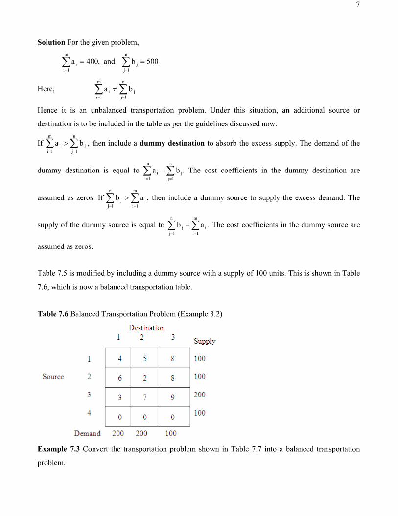
Table 7.5 is modified by including a dummy source with a supply of 100 units. This is shown in Table
7.6, which is now a balanced transportation table.
Table 7.6 Balanced Transportation Problem (Example 3.2)
Example 7.3 Convert the transportation problem shown in Table 7.7 into a balanced transportation
problem.

8
Solution We have
400band,500an
1jj
m
1ii == ∑∑
==
Here, ∑∑==
>n
1jj
m
1ii ba
It is unbalanced transportation problem. This is converted into balanced transportation by including a
dummy destination as shown in Table 7.8
TABLE 7.7 Example 7.3
TABLE 7.8 Balanced Transportation of Problem of Example 7.3
7.3 FINDING THE INITIAL BASIC SOLUTION
There are there method available to find initial feasible basic solution of transportation problem.
7.3.1. North West Corner Method(NWCM)
Algorithm for northwest corner cell method
Step 1: Find the minimum of the supply and demand values with respect to the current northwest corner
cell of the cost matrix.
9
Step 2: Allocate this minimum value to the current northwest corner cell and subtract this minimum
from the supply and demand values with respect to the current northwest corner cell.
Step 3: Check whether exactly one of the row/column corresponding to the northwest comer cell
has zero supply/demand, respectively. If so, go to step 4 otherwise, go to step 5.
Step 4: Delete that row/column with respect to the current northwest corner cell which has the zero
supply/demand and go to step 6.
Step 5: Delete both the row and the column with respect to the current northwest corner cell. Step 6:
Check whether exactly one row or column is left out. If yes, go to step 7 otherwise go to step 1.
Step 7: Match the supply/demand of that row/column with the remaining demands/supplies of the
undeleted columns/rows.
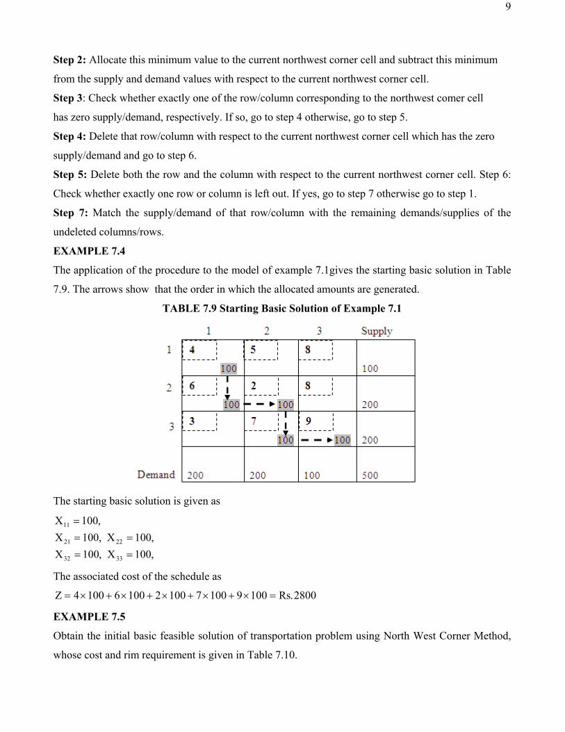
EXAMPLE 7.4
The application of the procedure to the model of example 7.1gives the starting basic solution in Table
7.9. The arrows show that the order in which the allocated amounts are generated.
TABLE 7.9 Starting Basic Solution of Example 7.1
The starting basic solution is given as
,100X,100X,100X,100X
,100X
3332
2221
11
====
=
The associated cost of the schedule as
2800.Rs10091007100210061004Z =×+×+×+×+×=
EXAMPLE 7.5
Obtain the initial basic feasible solution of transportation problem using North West Corner Method,
whose cost and rim requirement is given in Table 7.10.
10
TABLE 7.10 Cost Matrix of Example 7.5
D1 D2 D3 Supply
O1 2 7 4 5
O2 3 3 1 8
O3 5 4 7 7
O4 1 6 2 14
Demand 7 9 18 34
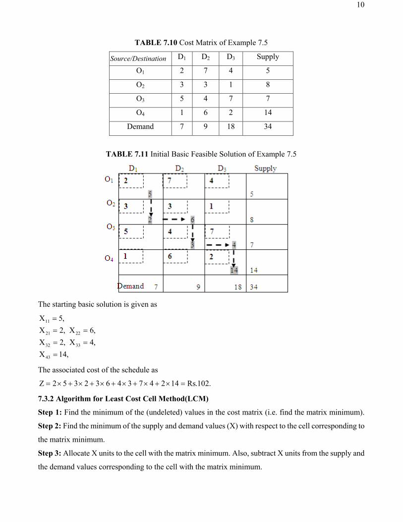
TABLE 7.11 Initial Basic Feasible Solution of Example 7.5
The starting basic solution is given as
,14X,4X,2X,6X,2X
,5X
43
3332
2221
11
=====
=
The associated cost of the schedule as
.102.Rs1424734632352Z =×+×+×+×+×+×=
7.3.2 Algorithm for Least Cost Cell Method(LCM)
Step 1: Find the minimum of the (undeleted) values in the cost matrix (i.e. find the matrix minimum).
Step 2: Find the minimum of the supply and demand values (X) with respect to the cell corresponding to
the matrix minimum.
Step 3: Allocate X units to the cell with the matrix minimum. Also, subtract X units from the supply and
the demand values corresponding to the cell with the matrix minimum.
Source/Destination
11
Step 4: Check whether exactly one of the row/column corresponding to the cell with the matrix
minimum has zero supply/zero demand, respectively. If yes, go to step 5 otherwise, go to step 6.
Step 5: Delete that row/column with respect to the cell with the matrix minimum which has the zero
supply/zero demand and go to step 7.
Step 6: Delete both the row and the column with respect to the cell with the matrix minimum.
Step 7: Check whether exactly one row or column is left out. If yes, go to step 8 otherwise, go to step 1.
Step 8: Match the supply/demand of that row/column with the remaining demands/supplies of the
undeleted columns/rows.
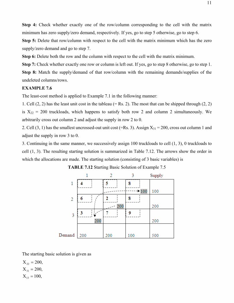
EXAMPLE 7.6
The least-cost method is applied to Example 7.1 in the following manner:
1. Cell (2, 2) has the least unit cost in the tableau (= Rs. 2). The most that can be shipped through (2, 2)
is X22 = 200 truckloads, which happens to satisfy both row 2 and column 2 simultaneously. We
arbitrarily cross out column 2 and adjust the supply in row 2 to 0.
2. Cell (3, 1) has the smallest uncrossed-out unit cost (=Rs. 3). Assign X31 = 200, cross out column 1 and
adjust the supply in row 3 to 0.
3. Continuing in the same manner, we successively assign 100 truckloads to cell (1, 3), 0 truckloads to
cell (1, 3). The resulting starting solution is summarized in Table 7.12. The arrows show the order in
which the allocations are made. The starting solution (consisting of 3 basic variables) is
TABLE 7.12 Starting Basic Solution of Example 7.5
The starting basic solution is given as
,100X,200X,200X
13
31
22
===
12
The associated cost of the schedule as
1800.Rs100820022003Z =×+×+×=
The quality of the least-cost starting solution is better than that of the northwest-corner method
(Example 7.5) because it yields a smaller value of Z (Rs. 83 versus Rs. 102 in the northwest-corner
method).
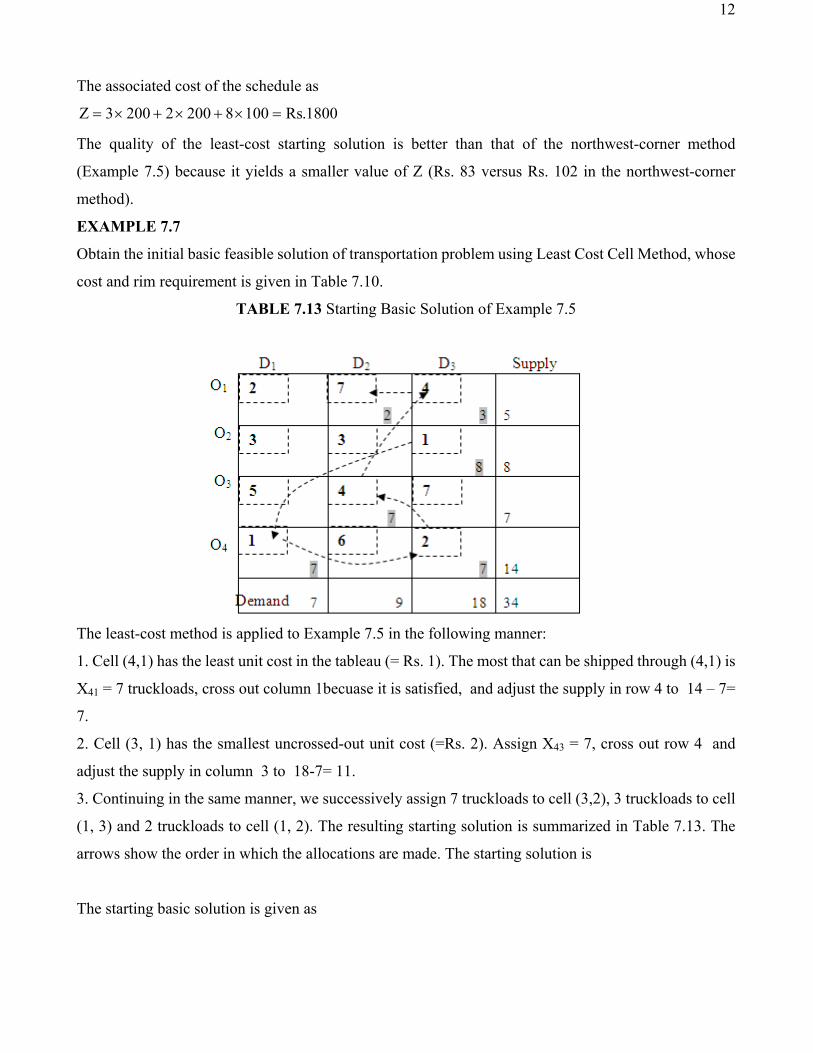
EXAMPLE 7.7
Obtain the initial basic feasible solution of transportation problem using Least Cost Cell Method, whose
cost and rim requirement is given in Table 7.10.
TABLE 7.13 Starting Basic Solution of Example 7.5
The least-cost method is applied to Example 7.5 in the following manner:
1. Cell (4,1) has the least unit cost in the tableau (= Rs. 1). The most that can be shipped through (4,1) is
X41 = 7 truckloads, cross out column 1becuase it is satisfied, and adjust the supply in row 4 to 14 – 7=
7.
2. Cell (3, 1) has the smallest uncrossed-out unit cost (=Rs. 2). Assign X43 = 7, cross out row 4 and
adjust the supply in column 3 to 18-7= 11.
3. Continuing in the same manner, we successively assign 7 truckloads to cell (3,2), 3 truckloads to cell
(1, 3) and 2 truckloads to cell (1, 2). The resulting starting solution is summarized in Table 7.13. The
arrows show the order in which the allocations are made. The starting solution is
The starting basic solution is given as

13
,7X,7X,7X,8X
,3X,2X
4341
32
23
1312
====
==
The associated cost of the schedule as 83.Rs727174813427Z =×+×+×+×+×+×=
The quality of the least-cost starting solution is better than that of the northwest-corner method
(Example 7.5) because it yields a smaller value of Z (Rs. 1800 versus Rs. 2800 in the northwest-corner
method).
7.3.3 Vogel's Approximation Method (VAM)
The steps involved in this method for finding the initial solution are as follows.
Step 1 Find the penalty cost, naively the difference between the smallest and next smallest costs in each
row and column.
Step 2 Among the penalties as found in step(l) choose the maximum penalty. If this maximum penalty is
more than one (i.e if there is a tie) choose any one arbitrarily.
Step 3 In the selected row or column as by step(2) find out the cell having the least cost. Allocate to this
cell as much as possible depending on the capacity and requirements.
Step 4 Delete the row or column which is fully exhausted. Again compute the column and row penalties
for the reduced transportation table and then go to step (2). Repeat the procedure until all the rim
requirements are satisfied.
Note If the column is exhausted, then there is a change in row penalty and vice versa.
EXAMPLE 7.8
Vogel’s Approximation Method is applied to Example 7.1, Table 7.3
TABLE 7.14 Starting Basic Solution of Example 7.1
14
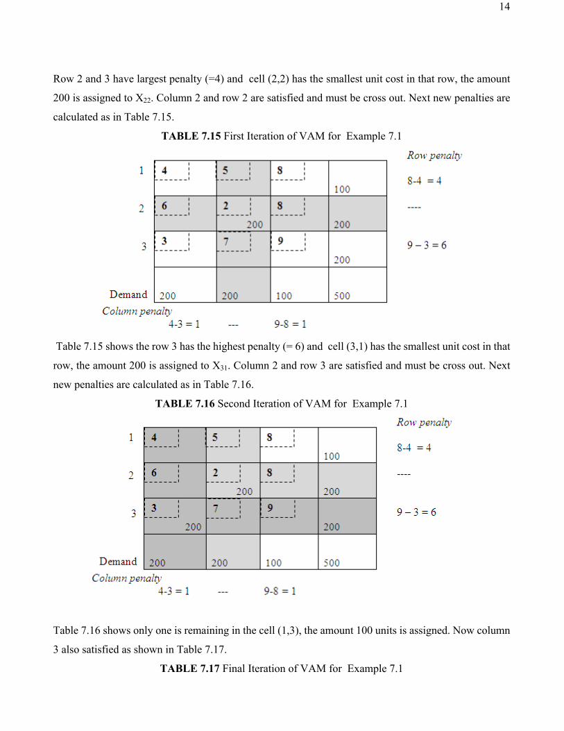
Row 2 and 3 have largest penalty (=4) and cell (2,2) has the smallest unit cost in that row, the amount
200 is assigned to X22. Column 2 and row 2 are satisfied and must be cross out. Next new penalties are
calculated as in Table 7.15.
TABLE 7.15 First Iteration of VAM for Example 7.1
Table 7.15 shows the row 3 has the highest penalty (= 6) and cell (3,1) has the smallest unit cost in that
row, the amount 200 is assigned to X31. Column 2 and row 3 are satisfied and must be cross out. Next
new penalties are calculated as in Table 7.16.
TABLE 7.16 Second Iteration of VAM for Example 7.1
Table 7.16 shows only one is remaining in the cell (1,3), the amount 100 units is assigned. Now column
3 also satisfied as shown in Table 7.17.
TABLE 7.17 Final Iteration of VAM for Example 7.1

15
The Associated cost of the schedule as 1800.Rs100820022003Z =×+×+×=
EXAMPLE 7.9
Vogel’s Approximation Method is applied to Example 7.5, Table 7.10
TABLE 7.18 First Iteration of VAM for Example 7.5
In Table 7.18, row penalties and column penalties are computed. The maximum of these penalties is 2
which occur in rows 1 and 2. Hence, the cell with the least cost in these rows are to be identified. This
occurs at the cell (2, 3). The supply and the demand values corresponding to the cell (2, 3) are 8 and 18,
respectively. The minimum of these values is 8. Thus 8 units are allocated to the cell (2, 3) and the same
is subtracted from the supply and demand values of the cell (2, 3).
In this process, the demand at the source 2 is fully satisfied. Hence, this row is highlighted and the
resultant data is shown in Table 7.19.
16
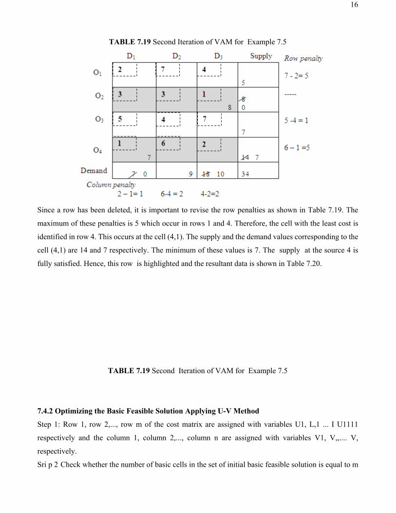
TABLE 7.19 Second Iteration of VAM for Example 7.5
Since a row has been deleted, it is important to revise the row penalties as shown in Table 7.19. The
maximum of these penalties is 5 which occur in rows 1 and 4. Therefore, the cell with the least cost is
identified in row 4. This occurs at the cell (4,1). The supply and the demand values corresponding to the
cell (4,1) are 14 and 7 respectively. The minimum of these values is 7. The supply at the source 4 is
fully satisfied. Hence, this row is highlighted and the resultant data is shown in Table 7.20.
TABLE 7.19 Second Iteration of VAM for Example 7.5
7.4.2 Optimizing the Basic Feasible Solution Applying U-V Method
Step 1: Row 1, row 2,..., row m of the cost matrix are assigned with variables U1, L,1 ... I U1111
respectively and the column 1, column 2,..., column n are assigned with variables V1, V,,.... V,
respectively.
Sri p 2 Check whether the number of basic cells in the set of initial basic feasible solution is equal to m

17
+ n – 1. If yes, go to step 4, otherwise, go to step 3.
Step 3 Convert the necessary number of non-basic cells into basic cells to satisfy the condition stated in
step 2 (while doing this, sufficient care should be taken such that there is no closed loop formation with
the inclusion of the new basic cell(s)). The concept of the closed loop is explained in step 8.
Step 4: Compute the values for U,, U,_,..., U,,,, and V1, I V,, by applying the following formula
2
to all the basic cells only.
U1 + Vi Cii (assume U, = 0)
Step 5: Compute penalties Pij for the non-basic cells by using the formula: P'j = Uj -+- Vi – cjj
Step 6: Check whether all P;j values are less than or equal to zero. If yes, go to step 12, otherwise, go to
step 7.
Step T Identify the non-basic cell which has the maximum positive penalty, and term that cell as the new
basic cell.
Step 8: Starting from the new cell, draw a closed loop consisting of only horizontal and vertical lines
passing through some basic cells. (Note: Change of direction of the loop should be with 90 degrees only
at some basic cell.)
Step 9: Starting from the new basic cell, alternatively assign positive (+) and negative (–) signs at the
corners of the closed loop.
Step 10: Find the minimum of the allocations made amongst the negatively signed cells.
Step 11: Obtain the table for the next iteration by doing the following steps and then go to step 2.
(i) Add the minimum allocation obtained in the previous step to all the positively signed cells and
subtract minimum allocation from all the negatively signed cells and then treat the net allocations as the
allocations in the corresponding cells of the next iteration.
(ii) Copy the allocations which are on the closed loop but not at the corner points of the closed loop, as
well as the allocations which are not on the loop as such without any modifications to the corresponding
cells of the next iteration.
Step 12. The optimality is reached. Treat the present allocations to the set of basic cells as the optimum
allocations.
Step 13. Stop.
Step 1 Starting with the cell at the upper left corner (North west) of the transportation matrix we allocate
as much as possible so that either the capacity of the first row is exhausted or the destination requirement

18
of the first column is satisfied i.e., ).b,amin(X 111i =
Step 2 If ,ab 11 > we move down vertically to the second row and make the second allocation of
magnitude ),Xb,amin(X 1i1222 −= in the cell (2, 1)
If ,ab 11 > move right horizontally to the second column and make the second allocation of magnitude
),bX,amin(X 11i112 −= in the cell (1, 2)
If 11 ab = b, there is a tie for the second allocation. We make the second allocations of magnitude
0)b,aamin(X 11112 =−= in cell (1,2)
or 0)bb,amin(X 11221 =−= in the cell (2,1)
Step 3 Repeat steps I and 2 moving down towards the lower right corner of the transportation table until
all the rim requirements are satisfied.
Example Obtain the initial basic feasible solution of a transportation problem whose cost and rim
requirement table is given below.
Example Determine an initial basic Feasible solution to the following transportation problem using
N.W.C.R
Origin/Ds D1 D2 D3 D4 Supply
O1 6 4 1 5 14
O2 8 9 2 7 16
O3 4 3 6 2 5
Required 6 10 15 4 35
Least Cost-or Matrix Minima Method
Step 1 Determine the smallest cost in the cost matrix of the transportation table.
Let it be ijC . Allocate ).b,amin(X 11ij = in the cell (i, j)
Step 2 If iij aX = cross off the ith row of the transportation table and decrease bj by ai. Then go to step3.
Origin\Destination D1 D2 D3 Supply
O1 2 7 4 5
O2 3 3 1 8
O3 5 4 7 7
O4 1 6 2 14
Demand 7 9 18 34
19
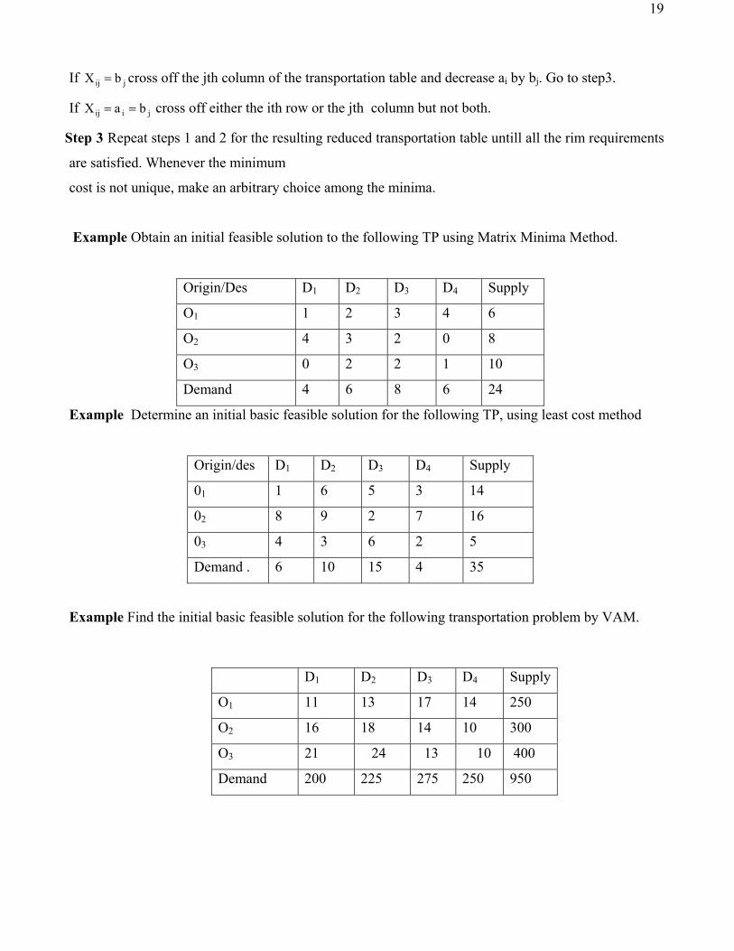
If jij bX = cross off the jth column of the transportation table and decrease ai by bj. Go to step3.
If jiij baX == cross off either the ith row or the jth column but not both.
Step 3 Repeat steps 1 and 2 for the resulting reduced transportation table untill all the rim requirements
are satisfied. Whenever the minimum
cost is not unique, make an arbitrary choice among the minima.
Example Obtain an initial feasible solution to the following TP using Matrix Minima Method.
Origin/Des D1 D2 D3 D4 Supply
O1 1 2 3 4 6
O2 4 3 2 0 8
O3 0 2 2 1 10
Demand 4 6 8 6 24
Example Determine an initial basic feasible solution for the following TP, using least cost method
Origin/des D1 D2 D3 D4 Supply
01 1 6 5 3 14
02 8 9 2 7 16
03 4 3 6 2 5
Demand . 6 10 15 4 35
Example Find the initial basic feasible solution for the following transportation problem by VAM.
D1 D2 D3 D4 Supply
O1 11 13 17 14 250
O2 16 18 14 10 300
O3 21 24 13 10 400
Demand 200 225 275 250 950
20
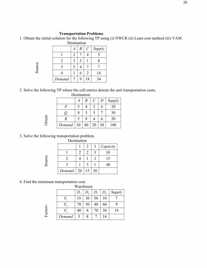
Transportation Problems 1. Obtain the initial solution for the following TP using (i) NWCR (ii) Least cost method (iii) VAM Destination
341897142614774538133254721
Demand
SupplyCBA
2. Solve the following TP where the cell entries denote the unit transportation costs. Destination
10030204010506495307538206245
DemandRQP
SupplyDCBA
3. Solve the following transportation problem. Destination
301520401313152142103221
321
Demand
Capacity
4. Find the minimum transportation cost. Warehouse
14785183070840960403070710503019
3
2
1
4321
DemandFFF
SupplyDDDD
Sour
ce
Orig
in
Sour
ce
Fact
ory
21
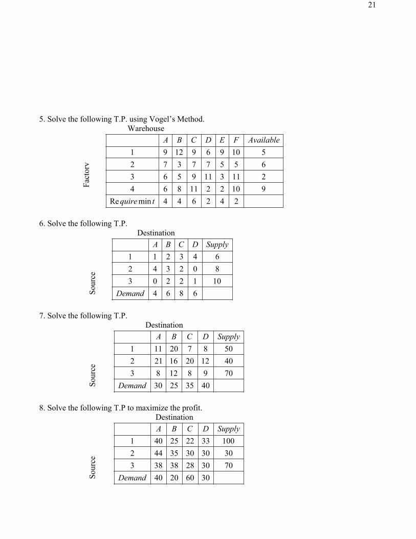
5. Solve the following T.P. using Vogel’s Method. Warehouse
242644minRe91022118642113119563655773725109691291
tquire
AvailableFEDCBA
6. Solve the following T.P. Destination
68641012203802342643211
Demand
SupplyDCBA
7. Solve the following T.P. Destination
403525307098128340122016212508720111
Demand
SupplyDCBA
8. Solve the following T.P to maximize the profit. Destination
306020407030283838330303035442
100332225401
Demand
SupplyDCBA
Fact
ory
Sour
ce
Sour
ce
Sour
ce
22
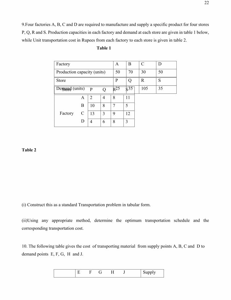
9.Four factories A, B, C and D are required to manufacture and supply a specific product for four stores
P, Q, R and S. Production capacities in each factory and demand at each store are given in table 1 below,
while Unit transportation cost in Rupees from each factory to each store is given in table 2.
Table 1
Table 2
(i) Construct this as a standard Transportation problem in tabular form.
(ii)Using any appropriate method, determine the optimum transportation schedule and the
corresponding transportation cost.
10. The following table gives the cost of transporting material from supply points A, B, C and D to
demand points E, F, G, H and J.
E F G H J Supply
Factory A B C D
Production capacity (units) 50 70 30 50
Store P Q R S
Demand (units) 25 35 105 35 Store P Q R S
Factory
A
B
C
D
2 4 8 11
10 8 7 5
13 3 9 12
4 6 8 3

23
A
B
C
D
8 10 12 17 15
15 13 18 11 9
14 20 6 10 13
13 19 7 6 12
100
150
180
280
Demand 90 170 50 210 190
The present allocation is as follows:
A to E 90, A to F 10, B to F 150, C to F 10, C to G 50, C to J 120, D to H 210, D to J
70.
(a) Check the allocation is optimum, if not find an optimum schedule.
(b) If in the above problem the transportation cost from A to G is reduced to 10, what will be the new
optimum schedule?.
(c) If the availability of supply point A is reduced by 10 units, use each of the following criteria to
obtain a initial basic feasible solution:
(i) Northwest corner rule
(ii) Least cost method
(d) Starting with best initial solution is found in part (c), obtain an optimal solution, and hence produce
transportation schedule.
11.Consider a transportation problem involving 3 sources and 3 destinations. Find minimum transportation cost.
400400200
183025
91210
151020
Supply
200
300500
1000
Destination1 2 3
Source
1
2
3
Demand
24
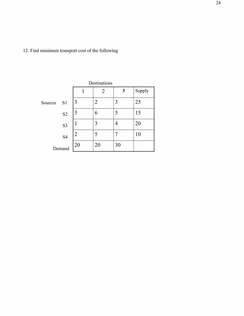
12. Find minimum transport cost of the following
302020
10752
20431
15565
25323
Supply321
Sources S1
S2
S3
S4
Demand
Destinations